Problems on Numerical Methods

for Engineers

Pedro Fortuny Ayuso

EPIG, Gijon. Universidad de OviedoE-mail address : fortunypedro@uniovi.es

CC© BY:© Copyright c© 2011–2015 Pedro Fortuny Ayuso

This work is licensed under the Creative Commons Attribution 3.0License. To view a copy of this license, visithttp://creativecommons.org/licenses/by/3.0/es/

or send a letter to Creative Commons, 444 Castro Street, Suite 900,Mountain View, California, 94041, USA.

CHAPTER 1

Arithmetic and Errors

Problem 1. The distance from the Earth to the Moon varies be-tween 356400km and 406700km. Give a bound on the absolute andrelative errors incurred when using one of both values as the “real dis-tance.” This requires giving two bounds

Problem 2 (The Gregorian Calendar). Explain the algorithm ofthe Gregorian Calendar, taking into account that

• A “real” year lasts 365.242374 days.• It is designed so that the mismatch between the Spring Equinox

and the 21st of March be never more than dos dıas.

Problem 3. The following integral∫ 1

0

e−x2

dx

is computed using Taylor’s polynomial of order 4 of the integrand,which is

T (e−x2

, x = 0, 4) = 1− x2 +x4

2.

Give an approximation to the absolute and relative errors incurred ifthe real value of the integral is 0.74682413+. ¿Are they remarkable?

Problem 4. When computing 1 − sin(π/2 + x) for small x, onecommits a specific type of error. Which one? Can this be prevented?

Problem 5. Compute the addition

4∑i=1

1

7i=

1

7+

1

72+

1

73+

1

74

in the following ways:

• Truncating all the operations to 3 decimal digits.• Rounding all the operations to 3 decimal digits.• Truncating all the operations to 4 significant figures.• Rounding all the operations to 4 significant figures.

Compute, in each case, the absolute and relative errors, if the exactvalue of the sum is 0.16659725.

3

4 1. ARITHMETIC AND ERRORS

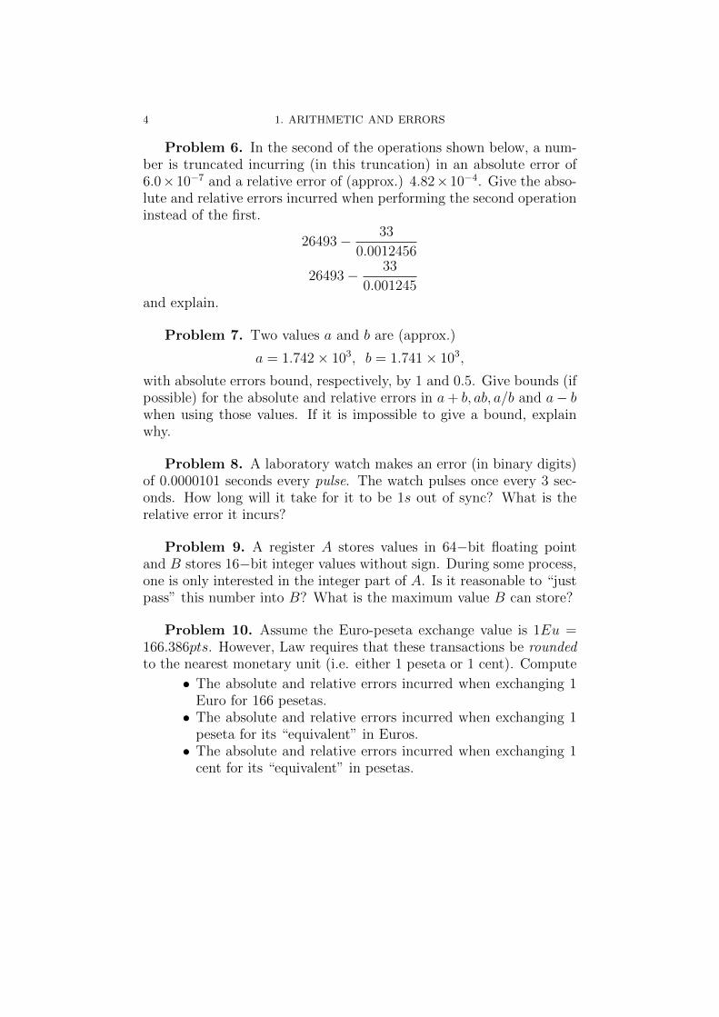
Problem 6. In the second of the operations shown below, a num-ber is truncated incurring (in this truncation) in an absolute error of6.0×10−7 and a relative error of (approx.) 4.82×10−4. Give the abso-lute and relative errors incurred when performing the second operationinstead of the first.

26493− 33

0.0012456

26493− 33

0.001245and explain.

Problem 7. Two values a and b are (approx.)

a = 1.742× 103, b = 1.741× 103,

with absolute errors bound, respectively, by 1 and 0.5. Give bounds (ifpossible) for the absolute and relative errors in a+ b, ab, a/b and a− bwhen using those values. If it is impossible to give a bound, explainwhy.

Problem 8. A laboratory watch makes an error (in binary digits)of 0.0000101 seconds every pulse. The watch pulses once every 3 sec-onds. How long will it take for it to be 1s out of sync? What is therelative error it incurs?

Problem 9. A register A stores values in 64−bit floating pointand B stores 16−bit integer values without sign. During some process,one is only interested in the integer part of A. Is it reasonable to “justpass” this number into B? What is the maximum value B can store?

Problem 10. Assume the Euro-peseta exchange value is 1Eu =166.386pts. However, Law requires that these transactions be roundedto the nearest monetary unit (i.e. either 1 peseta or 1 cent). Compute

• The absolute and relative errors incurred when exchanging 1Euro for 166 pesetas.• The absolute and relative errors incurred when exchanging 1

peseta for its “equivalent” in Euros.• The absolute and relative errors incurred when exchanging 1

cent for its “equivalent” in pesetas.

CHAPTER 2

Solutions to Nonlinear Equations

Problem 11. Use the Babilonian algorithm for square roots tocompute

√600 and

√1000 so that the error when squaring be less than

0.1.

Problem 12. Explain the relation between the Babilonian algo-rithm for square roots and Newton-Raphson’s.

Problem 13. Use three steps of Newton-Raphson’s method forcomputing an approximation of

√5, with x0 = 1. Can you guarantee

—without computing more steps— that |x6 −√

5| < 0.0001 [explain]?

Problem 14. What happens if one runs Newton-Raphson’s algo-rithm for the function f(x) = x3 − x and seed x0 =

√1/5? Explain.

Problem 15. Compare the convergence speed of the Bisection al-gorithm in and Newton-Raphson’s with seed 0.9 for f(x) = x7− 0.9 in[0, 1].

Problem 16. Explain what happens if Newton-Raphson’s algo-rithm is used with seed x0 = 3 for f(x) = atan(x)− .3. Can anythingbe done about it?

Problem 17. Perform two iterations of the secant algorithm forf(x) = tan(x) + .5 with seeds 0 and 0.1.

Problem 18. Compute with 5 exact digits (using Newton-Raphson’salgorithm) a root of cos(3x)− x. Does this question make sense if onecannot compute the values of trigonometric functions exactly? Cananything be done about it?

Problem 19. Compute approximate roots to f(x) = cos(3x) − xusing Newton-Raphson. Make sure that at least 4 decimal digits areexact.

Problem 20. Consider the functions verifying

f(x)

f ′(x)= 3x.

5

6 2. SOLUTIONS TO NONLINEAR EQUATIONS

without solving the differential equation, explain what happens toNewton-Raphson’s algorithm when applied to them.

Problem 21. Consider g(x) = π + 12

sin(x2) and f(x) = g(x)− x.

• Verify that f has a single root c and that it is between 0 and2π.• Compute an approximate value of c using Newton-Raphson’s

algorithm.• Compute an approximate value of c with at least 5 exact fig-

ures using any algorithm and explaining why those are exactfigures.

Problem 22. Try to use the fixed point algorithm to compute aroot of f(x) = cos(x) − x betwen x = 0 and x = 1 (notice that theinterval [0, 1] will not be the most useful one). Compare its convergencespeed with that of the bisection algorithm and Newton-Raphson’s.

Problem 23. Let us describe the regula falsi algorithm as that inwhich, in order to approximate a root of a continuous function f in[a, b] in which f(a)f(b) < 0, one starts with a and b and at each step,one substitutes either (depending on the sign of f) by the meetingpoint of OX with the line joining (a, f(a)) and (b, f(b)). Describe itwith precision.

Problem 24. Could it happen that, at some step in Newton-Raphson’s algorithm one had |xn+1−xn| < 10−7 and also f(xn+1) > 1?Why?

Problem 25. Let f : [0, 2] → [0, 2] be a differentiable functionsuch that f(0) = 1.5, f(1) = 0 and f(2) = 0.5. Does it satisfy thefixed point convergence conditions? Has it got any fixed point? Why?

Problem 26. Explain why Newton-Raphson’s algorithm appliedto f(x) = atan(x) will always diverge if |x0| > 10. Clue: atan(10) >√

2.

Problem 27. Use two steps of Newton-Raphson’s method for com-puting an approximation of 3

√2, with x0 = 1. Can you guarantee

—without computing more steps— that |x3 − 3√

2| < 0.001?

CHAPTER 3

Solutions to Linear Systems

Problem 28. Consider the following n× n square matrix:

A =

1 −1 0 0 . . . 01 0 −1 0 . . . 01 0 0 −1 . . . 0...

......

.... . .

...1 0 0 0 . . . −11 0 0 0 . . . 0

.

Perform the following:

• Compute its determinant.• Explain to what kind of intermediate matrices Gauss’ algo-

rithm will give rise.• Compute the LU decomposition of A.• Solve the system Ax = b in a more efficient way, for any b.

Problem 29. Explain what happens if Gauss’ method with partialpivoting is applied to an n×n singular matrix. And what if no pivotingis used?

Problem 30. Consider a system of linear equations Ax = b whoseentries have been obtained from measurements with 4 digits of preci-sion. The matrix A is such that κ∞(A) = 400. Comment.

Problem 31. Verify that the condition number for the infinitynorm of the following n× n matrix

Bn =

1 −1 −1 . . . −10 1 −1 . . . −10 0 1 . . . −1...

......

. . ....

0 0 0 . . . 1

is κ∞(Bn) = n2n−1. Is it well-conditioned? However, is it difficult tosolve a system Bnx = b?

Problem 32. Is the determinant of a matrix related in any way toits condition number? Why?

7

8 3. SOLUTIONS TO LINEAR SYSTEMS

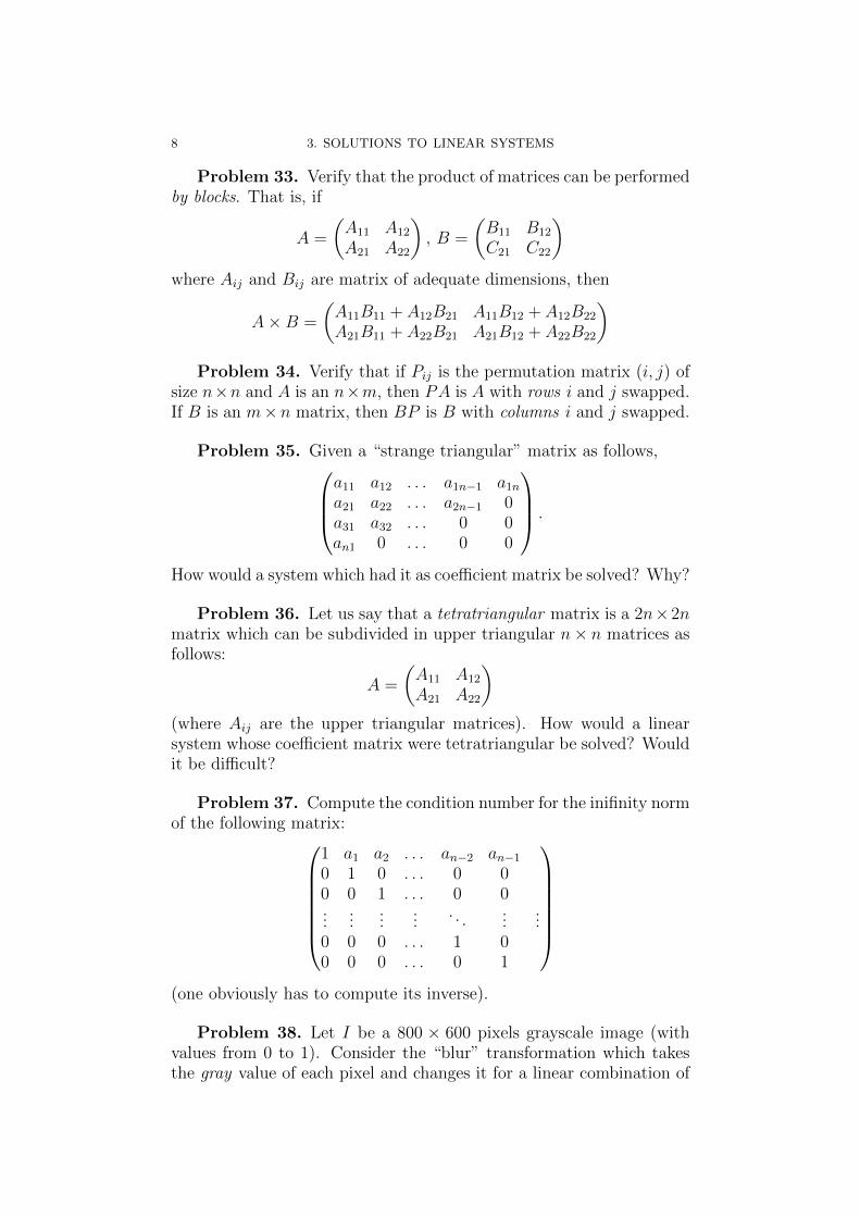
Problem 33. Verify that the product of matrices can be performedby blocks. That is, if

A =

(A11 A12

A21 A22

), B =

(B11 B12

C21 C22

)where Aij and Bij are matrix of adequate dimensions, then

A×B =

(A11B11 + A12B21 A11B12 + A12B22

A21B11 + A22B21 A21B12 + A22B22

)Problem 34. Verify that if Pij is the permutation matrix (i, j) of

size n×n and A is an n×m, then PA is A with rows i and j swapped.If B is an m×n matrix, then BP is B with columns i and j swapped.

Problem 35. Given a “strange triangular” matrix as follows,a11 a12 . . . a1n−1 a1na21 a22 . . . a2n−1 0a31 a32 . . . 0 0an1 0 . . . 0 0

.

How would a system which had it as coefficient matrix be solved? Why?

Problem 36. Let us say that a tetratriangular matrix is a 2n×2nmatrix which can be subdivided in upper triangular n× n matrices asfollows:

A =

(A11 A12

A21 A22

)(where Aij are the upper triangular matrices). How would a linearsystem whose coefficient matrix were tetratriangular be solved? Wouldit be difficult?

Problem 37. Compute the condition number for the inifinity normof the following matrix:

1 a1 a2 . . . an−2 an−10 1 0 . . . 0 00 0 1 . . . 0 0...

......

.... . .

......

0 0 0 . . . 1 00 0 0 . . . 0 1

(one obviously has to compute its inverse).

Problem 38. Let I be a 800 × 600 pixels grayscale image (withvalues from 0 to 1). Consider the “blur” transformation which takesthe gray value of each pixel and changes it for a linear combination of

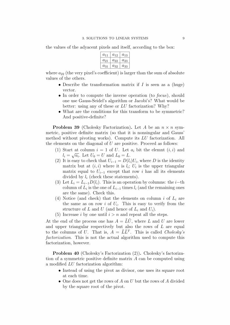
3. SOLUTIONS TO LINEAR SYSTEMS 9

the values of the adyacent pixels and itself, according to the box:

a11 a12 a13a21 a22 a23a31 a32 a33

where a22 (the very pixel’s coefficient) is larger than the sum of absolutevalues of the others.

• Describe the transformation matrix if I is seen as a (huge)vector.• In order to compute the inverse operation (to focus), should

one use Gauss-Seidel’s algorithm or Jacobi’s? What would bebetter: using any of these or LU factorization? Why?• What are the conditions for this transform to be symmetric?

And positive-definite?

Problem 39 (Cholesky Factorization). Let A be an n × n sym-metric, positive definite matrix (so that it is nonsingular and Gauss’method without pivoting works). Compute its LU factorization. Allthe elements on the diagonal of U are positive. Proceed as follows:

(1) Start at column i = 1 of U . Let ai bit the elemnt (i, i) andli =√ai. Let U0 = U and L0 = L.

(2) It is easy to check that Ui−1 = D(li)Ui, where D is the identitymatrix but at (i, i) where it is li; Ui is the upper triangularmatrix equal to Ui−1 except that row i has all its elementsdivided by li (check these statements).

(3) Let Li = Li−1D(li). This is an operation by columns: the i−thcolumn of Li is the one of Li−1 times li (and the remaining onesare the same). Check this.

(4) Notice (and check) that the elements on column i of Li arethe same as on row i of Ui. This is easy to verify from thestructure of L and U (and hence of Li and Ui).

(5) Increase i by one until i > n and repeat all the steps.

At the end of the process one has A = LU , where L and U are lowerand upper triangular respectively but also the rows of L are equalto the columns of U . That is, A = LLT . This is called Cholesky’sfactorization. This is not the actual algorithm used to compute thisfactorization, however.

Problem 40 (Cholesky’s Factorization (2)). Cholesky’s factoriza-tion of a symmetric positive definite matrix A can be computed usinga modified LU factorization algorithm:

• Instead of using the pivot as divisor, one uses its square rootat each time.• One does not get the rows of A on U but the rows of A divided

by the square root of the pivot.

10 3. SOLUTIONS TO LINEAR SYSTEMS

• On the diagonal of L one gets also the square root of the pivotsand on its columns, the multipliers.• As A is symmetric and positive definite, one gets L = UT at

the end.

This is the way to compute Cholesky’s factorization: it takes advantageof the properties of A, which need to be known in advance.

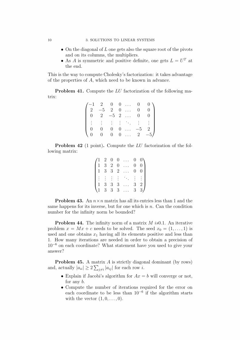
Problem 41. Compute the LU factorization of the following ma-trix:

−1 2 0 0 . . . 0 02 −5 2 0 . . . 0 00 2 −5 2 . . . 0 0...

......

.... . .

......

0 0 0 0 . . . −5 20 0 0 0 . . . 2 −5

Problem 42 (1 point). Compute the LU factorization of the fol-

lowing matrix:

1 2 0 0 . . . 0 01 3 2 0 . . . 0 01 3 3 2 . . . 0 0...

......

.... . .

......

1 3 3 3 . . . 3 21 3 3 3 . . . 3 3

Problem 43. An n×n matrix has all its entries less than 1 and the

same happens for its inverse, but for one which is n. Can the conditionnumber for the infinity norm be bounded?

Problem 44. The infinity norm of a matrix M is0.1. An iterativeproblem x = Mx + c needs to be solved. The seed x0 = (1, . . . , 1) isused and one obtains x1 having all its elements positive and less than1. How many iterations are needed in order to obtain a precision of10−6 on each coordinate? What statement have you used to give youranswer?

Problem 45. A matrix A is strictly diagonal dominant (by rows)and, actually |aii| ≥ 2

∑j 6=i |aij| for each row i.

• Explain if Jacobi’s algorithm for Ax = b will converge or not,for any b.• Compute the number of iterations required for the error on

each coordinate to be less than 10−6 if the algorithm startswith the vector (1, 0, . . . , 0).

3. SOLUTIONS TO LINEAR SYSTEMS 11

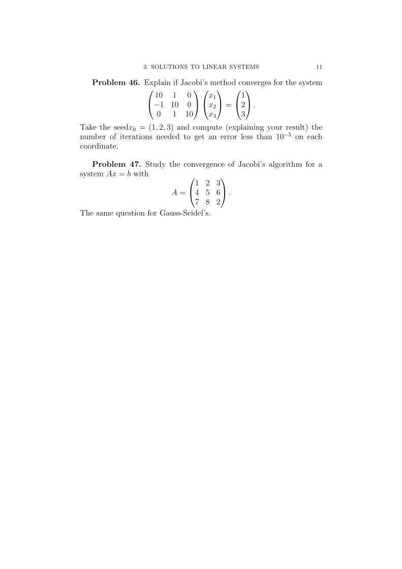
Problem 46. Explain if Jacobi’s method converges for the system10 1 0−1 10 00 1 10

x1x2x3

=

123

.

Take the seedx0 = (1, 2, 3) and compute (explaining your result) thenumber of iterations needed to get an error less than 10−5 on eachcoordinate.

Problem 47. Study the convergence of Jacobi’s algorithm for asystem Ax = b with

A =

1 2 34 5 67 8 2

.

The same question for Gauss-Seidel’s.

CHAPTER 4

Interpolation

Problem 48. Given four points on the plain, a degree two spline isto be built so that the derivative at the intermediate points is continous.Compute the ecuations which describe this problem (do not solve them)and explain whether the system is consisten and whether it has a uniquesolution or not. If it is not, give some extra equations which make itso.

Problem 49. Is it true that the greater number of points the nearerthe Lagrange interpolation polynomial is to the graph of the functionto be interpolated? Explain.

Problem 50. Would you use the Lagrange interpolation polyno-mial to approximate the function f(x) = ex given 5 values? Why?

Problem 51. Given a cloud of 1000 points (coordinates (x, y)), onewishes to interpolate it using least squares for the functions f(x) = 1,g(x) = x y h(x) = x2. Can it be done? What size is the linear systemto be solved?

Problem 52. A cloud of 300 points (coordinates (x, y)) is suchthat there exists a function f(x) = aebx for which the total quadraticerror is 0.1. Given the cloud (x, log(y)), the least squares interpolationfor the functions 1, x; is 2+3x. Can it be that the total quadratic errorof e2e3x for the original cloud be greater than 0.1. Why?

Problem 53. Compute the Lagrange basis polynomials for the fol-lowing points: (0, 2), (1, 3), (2, 4), (3, 10), (4, 20) and use them to com-pute the Lagrange interpolation polynomial of degree 4 passing throughthem.

Problem 54. Compute the Lagrange interpolation polynomial forthe points (0, 0), (1, 2), (2, 0).

Problem 55 (1 point). Compute the Lagrange interpolation poly-nomial for the points (0, 0), (1, 1), (2, 3).

13

14 4. INTERPOLATION

Problem 56 (1 point). A table shows the values at different timesof the speeds of a rocket. What kind of interpolation would you use tojoin them? Why?

Problem 57. Write the system of linear equations correspondingto the least squares interpolation problem for the cloud (0, 1), (1, 2), (2, 0), (3, 4), (5,−1)and the functions f(x) = x, g(x) = x2, h(x) = x4. Do not solve it.

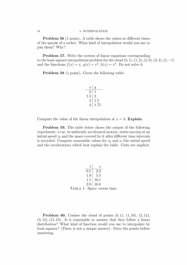
Problem 58 (1 point). Given the following table:

x y0 1

1.5 22 1.54 1.75

Compute the value of the linear interpolation at x = 3. Explain.

Problem 59. The table below shows the output of the followingexperiment: a car, in uniformly accelerated motion, starts moving at aninitial speed v0 and the space covered by it after different time intervalsis recorded. Compute reasonable values for v0 and a (the initial speedand the acceleration) which best explain the table. Units are implicit.

t s0.5 2.21.0 5.51.5 10.12.0 16.0

Tabla 1. Space versus time.

Problem 60. Coniser the cloud of points (0, 1), (1, 10), (2, 11),(3, 12), (12, 13). Is it reasonable to assume that they follow a lineardistribution? What kind of function would you use to interpolate byleast squares? (There is not a unique answer). Draw the points beforeanswering.

4. INTERPOLATION 15

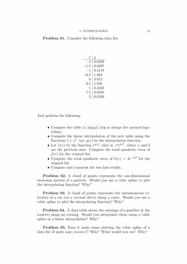
Problem 61. Consider the following data list:

x y−2 0.0338−1.5 0.0397−1 0.4119−0.5 1.862

0 3.0130.5 1.856

1 0.42401.5 0.0485

2 0.0249

And perform the following:

• Compute the table (x, log(y)) (log is always the natural loga-rithm).• Compute the linear interpolation of the new table using the

functions 1 y x2. Let g(x) be the interpolation function.

• Let f(x) be the function eg(x), that is, eaebx2, where a and b

are the previous ones. Compute the total quadratic error off(x) for the original list.

• Compute the total quadratic error of h(x) = 3e−2x2

for theoriginal list.• Compare and comment the two last results.

Problem 62. A cloud of points represents the one-dimensionalbrownian motion of a particle. Would you use a cubic spline to plotthe interpolating function? Why?

Problem 63. A cloud of points represents the instantaneous ve-locities of a car (on a normal drive) along a route. Would you use acubic spline to plot the interpolating function? Why?

Problem 64. A data table shows the earnings of a gambler at theroulette along an evening. Would you interpolate them using a cubicspline or a linear interpolation? Why?

Problem 65. Does it make sense plotting the cubic spline of adata list of pairs (age, income)? Why? What would you use? Why?

16 4. INTERPOLATION

Problem 66. State the equations required to solve the naturalcubic spline which interpolates the following data table:

x y0 11 32 03 44 5

Same question for the not-a-knot spline. If you have a computer handy,solve the systems and plot both splines.

Problem 67 (1 point). Given the following table:

x y0 1

1.5 22 1.54 1.75

Compute the value of the linear interpolation at x = 3. Explain.

Problem 68 (1 point). A table shows the values at different timesof the earnings (or losses) of a gambler at a roulette table during anevening. Would you use a linear interpolation or a cubic spline to plotthe graph? Why?

Problem 69. A cloud of 200 points is to be approximated by afunction of the form f(x) = a + b sin(x) + c cos(x). Explain what sizethe linear system of equations obtained has. Same question but f(x)being a polynomial in x of degree 10.

Problem 70. A function f : [0, 10]→ R is four times differentiableand |f 4)|(x) < 1 for x ∈ [0, 10]. It is approximated by a natural cubicspline s(x) with nodes at xi = i for i = 0, . . . , 10. What is the maximumerror between f(x) and s(x). Give a bound for the difference between∫ 10

0f(x) dx and

∫ 10

0s(x) dx.

Problem 71. How many nodes are necessary between 0 and 2π sothat the clamped cubic spline approximates the function sin(x) withan error of at most 10−6?

Problem 72. Would you use a clamped or a natural cubic splineto approximate the function sin(x) between 0 and 2π? Why?

CHAPTER 5

Numerical differentiation and integration

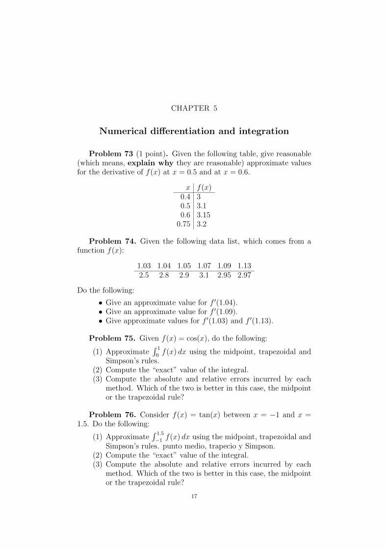
Problem 73 (1 point). Given the following table, give reasonable(which means, explain why they are reasonable) approximate valuesfor the derivative of f(x) at x = 0.5 and at x = 0.6.

x f(x)0.4 30.5 3.10.6 3.15

0.75 3.2

Problem 74. Given the following data list, which comes from afunction f(x):

1.03 1.04 1.05 1.07 1.09 1.132.5 2.8 2.9 3.1 2.95 2.97

Do the following:

• Give an approximate value for f ′(1.04).• Give an approximate value for f ′(1.09).• Give approximate values for f ′(1.03) and f ′(1.13).

Problem 75. Given f(x) = cos(x), do the following:

(1) Approximate∫ 1

0f(x) dx using the midpoint, trapezoidal and

Simpson’s rules.(2) Compute the “exact” value of the integral.(3) Compute the absolute and relative errors incurred by each

method. Which of the two is better in this case, the midpointor the trapezoidal rule?

Problem 76. Consider f(x) = tan(x) between x = −1 and x =1.5. Do the following:

(1) Approximate∫ 1.5

−1 f(x) dx using the midpoint, trapezoidal andSimpson’s rules. punto medio, trapecio y Simpson.

(2) Compute the “exact” value of the integral.(3) Compute the absolute and relative errors incurred by each

method. Which of the two is better in this case, the midpointor the trapezoidal rule?

17

18 5. NUMERICAL DIFFERENTIATION AND INTEGRATION

Problem 77. The density of a metallic bar is described by thefunction f(x) = sin(x)/x, for x from 1 to 3. Do the following:

(1) Approximate the mass using the midpoint, trapezoidal andSimpson’s rules.

(2) Same computation but dividing the interval into 3 subintervalsand applying the composite rules in each case.

Problem 78. Let f(x) = x7− 15x3 + 10x for from −2 to 2. Com-pute approximations to the integral between those two endpoints using:

• The simple midpoint, trapezoidal and Simpson’s rules.• The composite rules dividing the interval first into 2 and then

into 3 subintervals (that is, this part has to be done twice).• Compute all the absolute and relative errors incurred in each

case.

Problem 79. Compute, using the midpoint rule and Simpson’srule, approximations to the following integral∫ 1

0

ex dx.

Compute the exact value of the integral and give the absolute andrelative errors incurred with each method.

Problem 80 (1 point). Compute the following integral using thesimple midpoint, trapeze and Simpson’s rules:∫ 2π

0

sin2(x) dx.

The exact value is π. Explain what you would do to get a better ap-proximation. (There are no points for the computation of the integral,this question deals only with the explanation).

Problem 81. Consider f(x) = (1−x)x2(x+ 1) = −x4 +x2. Com-pute ∫ 1

−1f(x) dx

by hand and using Simpson’s, the Midpoint and the Trapezoidal rules(1 point). Explain what is happenning and what you can do to improvethe result (1 point).

Problem 82. Consider f(x) = 10(1−x)x2(x+1) = −10x4 +10x2.Compute ∫ 1

−1f(x) dx

5. NUMERICAL DIFFERENTIATION AND INTEGRATION 19

by hand and using Simpson’s and the Trapezoidal rules (0.75 point).Explain what is happenning and what you can do to improve the ap-proximations (0.75 point).

CHAPTER 6

Differential Equations

Problem 83. Consider the following initial-value problems. Foreach of them, verify that the proposed solution is valid for any value ofthe constant and compute the constant suitable for the initial condition.

• y′ = 0.03y for t ∈ [0, 1], with y(0) = 1000. Solution: y(t) =ke0.03t.• y′ = t/y for t ∈ [0, 1], with y(0) = 1. Solution: y(t) =

√t2 + k.

• y′ = e−y for t ∈ [1, 3], with y(1) = 0. Solution: y(t) = ln(t+k).• y′ = y/t2 for t ∈ [1, 2], with y(1) = 1. Solution: y(t) = ke−1/t.• y′ = 2t for t ∈ [0, 2], with y(0) = 1. Solution: y(t) = t2 + k.• y′ = y2 for t ∈ [0, 1/2], with y(0) = 1. Solution: y(t) =

1/(k − t).

Problem 84. For each of the problems in 83, do the following:

(1) Solve it (approximately) using Euler’s algorithm with two stepsof equal length.

(2) Compute the absolute and relative errors incurred at the lastpoint.

(3) Solve with four steps of equal length and compare.

Problem 85. For each of the problems in exercise 83, do:

(1) Solve it using Euler’s Modified Algorithm using two evenlyspaced steps.

(2) Compute the absolute and relative errors at the last step.(3) Same for four steps.

Problem 86. For each of the problems in exercise 83, do:

(1) Solve it using Heun’s Algorithm using two evenly spaced steps.(2) Compute the absolute and relative errors at the last step.(3) Same for four steps.

Problem 87. Consider the differential equation:

y′ = x2 + y2.

Can you decide whether the solutions are increasing/decreasing? Lety(x) be the solution satisfying y(0) = 1. Is it concave or convex? Hasit got any critical point?

Same questions for the solution with y(0) = −1.

21

22 6. DIFFERENTIAL EQUATIONS

Problem 88. Consider the differential equation:

y′ = y.

and let y(x) be the solution to the initial value problem y(−1) = 2. Isy(x) increasing? Has it got any critical point? Is it concave or convex?

Same questions for the solution with y(−1) = −2.What about the solution with y(−1) = 0?

Problem 89. Consider the differential equation:

y′ = sin(y).

Can you say anything about the points where its solutions have a max-imum or a minimum? And about their concavity/convexity?

Problem 90. Consider the differential equation:

y′ = (x− 1)y.

And let y1(x) be the solution to the initial value problem y(0) = −1.Has it got any critical points? In case it has, are they local maxima,minima or inflection points?

Same questions for the solution such that y(1) = 2.

Problem 91. Compute one step of the approximate solution tothe following initial value problem, using Heun’s method with h = 0.1: x = y x(0) = 0

y = −x y(0) = 1z = 1 z(0) = 0

The true solution is x(t) = sin(t), y(t) = cos(t), z(t) = t. Explain whatkind of trajectory this equation describes.

Problem 92. A cup full of tea is left cooling at the window, whichis at 0◦. It is known that it cools at a speed which —in adequateunits— is half the temperature. It starts at 70◦. Compute, usingEuler’s method with two steps, the approximate temperature after 2seconds. If the right answer is 25.752◦, what are the absolute andrelative errors?

Problem 93. There is a mass of a specific material which is leftto its own. It is known that it disintegrates at a rate which is 0.1the amount of mass at each moment. The experiment starts with 1kg.Compute, using Euler’s method with two steps, the amount of massafter 2 seconds. If the exact value is 0.819kg, what are the absoluteand relative errors incurred?

Problem 94. A projectile is thrown in the air with an initial speed(in (x, y) coordinates) of (1, 1) —in adequate units. The only active

6. DIFFERENTIAL EQUATIONS 23

forces are gravity and friction. Use g = 10 and consider that frictionis proportional to the speed but in the opposite direction, with pro-portionality constant 0.05. Use Heun’s method (one step) to give anapproximation to the position of the projectile after one second. As-sume that the initial position is (0, 0) in an adequate reference system.

Problem 95. Some salt is diluted in a pool of water of volume1000l, at a concentration of 0.1g/l. Water flows in and out of the pool at3l/s but the inflow contains salt at 0.3g/l. Compute the concentrationof salt in the pool after 2s and how long will it take for it to be 0.2g/l.Perform also the first computation in an approximate way using Euler’sand Heun’s method with 2 steps. For each calculation, give the absoluteand relative errors.

Problem 96. In a specific plot of land there live two species ofinsects, one which serves as food for the other, let us say ants andspiders. Ants reproduce exponentially at a rate 0.1 and only die asa consequence of being eaten, with a likelyhood of 0.07. Spiders diewith a likelyhood of 0.05 and breed proportionally to the likelyhood offeeding, with a proportionality constant 0.03. Spiders are counted inunits while ants are in thousands. Write down the appropriate ordinarydifferential equation describing this simplistic model and, using Euler’smethod, compute its state after 2 seconds using 2 steps, assumingthat the initial populations are 30000 ants and 10 spiders. Performa computer simulation with smaller steps and a longer time range.

Problem 97. The spread of an infectious disease can be simulatedwith the following (very simplistic) model (called the SIR model). LetS(t) be the “susceptible population”, that is, those individuals whocan be infected, I(t) the “infected population”, those that have beeninfected but are not cured and R(t) the “removed” population, thosethat were infected and are now cured (and will not be infected again);if the disease is mortal, R(t) includes the deceased individuals. Theflow of individuals, when happens, is S → I → R, obviously. Let usassume that the population is constant, that is N = S(t) + I(t) +R(t)is a fixed number. Then the model can be stated as

dS

dt= −βSI

NdI

dt= β

SI

N− γI

dR

dt= γI

Using Euler’s method, compute two steps for an initial state of S =10000, I = 20, R = 0 and values β = 0.02, γ = 0.05, time intervals

24 6. DIFFERENTIAL EQUATIONS

of 1. Perform a computer simulation for a long timespan of that sameproblem.