Probabilistic Wind Speed Forecasting using Ensembles

and Bayesian Model Averaging

J. McLean Sloughter, Tilmann Gneiting, and Adrian E. Raftery 1

Department of Statistics, University of Washington, Seattle, Washington, USA

Technical Report no. 544Department of Statistics

University of Washington

October 14, 2008

1J. McLean Sloughter (Email: mclean@stat.washington.edu) is a graduate student, TilmannGneiting (Email: tilmann@stat.washington.edu) is Professor of Statistics, and Adrian E. Raftery(Email: raftery@u.washington.edu) is Blumstein-Jordan Professor of Statistics and Sociology, all atthe Department of Statistics, University of Washington, Seattle, WA 98195-4322. We are grateful toJeff Baars, Chris Fraley, Eric Grimit, and Clifford F. Mass for helpful discussions and for providingcode and data. This research was supported by the DoD Multidisciplinary University ResearchInitiative (MURI) program administered by the Office of Naval Research under Grant N00014-01-10745, by the National Science Foundation under Awards ATM-0724721 and DMS-0706745, and bythe Joint Ensemble Forecasting System (JEFS) under subcontract S06-47225 from the UniversityCorporation for Atmospheric Research (UCAR).

Abstract

Probabilistic forecasts of wind speed are becoming critical as interest grows in wind as aclean and renewable source of energy, in addition to a wide range of other uses, from avia-tion to recreational boating. Statistical approaches to wind forecasting offer two particularchallenges: the distribution of wind speeds is highly skewed, and wind observations are re-ported to the nearest whole knot, a much coarser discretization than is seen in other weatherquantities. The prevailing paradigm in weather forecasting is to issue deterministic forecastsbased on numerical weather prediction models. Uncertainty can then be assessed throughensemble forecasts, where multiple estimates of the current state of the atmosphere are usedto generate a collection of deterministic predictions. Ensemble forecasts are often uncali-brated, however, and Bayesian model averaging (BMA) is a statistical way of postprocessingthese forecast ensembles to create calibrated predictive probability density functions (PDFs).It represents the predictive PDF as a weighted average of PDFs centered on the individualbias-corrected forecasts, where the weights reflect the forecasts’ relative contributions to pre-dictive skill over a training period. In this paper we extend BMA to provide probabilisticforecasts of wind speed, taking account of the skewness of the predictive distributions andthe discreteness of the observations. The BMA method is applied to 48-hour ahead fore-casts of maximum wind speed over the North American Pacific Northwest in 2003 usingthe University of Washington mesoscale ensemble, and is shown to provide calibrated andsharp probabilistic forecasts. Comparisons are made between a number of formulations thataccount for the discretization of the observations.

Contents

1 Introduction 1

2 Data and Methods 3

2.1 Forecast and observation data . . . . . . . . . . . . . . . . . . . . . . . . . . 32.2 Bayesian model averaging . . . . . . . . . . . . . . . . . . . . . . . . . . . . 42.3 Gamma model . . . . . . . . . . . . . . . . . . . . . . . . . . . . . . . . . . . 42.4 Parameter estimation . . . . . . . . . . . . . . . . . . . . . . . . . . . . . . . 5

2.4.1 Standard method . . . . . . . . . . . . . . . . . . . . . . . . . . . . . 62.4.2 Fully discretized method . . . . . . . . . . . . . . . . . . . . . . . . . 72.4.3 Doubly discretized method . . . . . . . . . . . . . . . . . . . . . . . . 82.4.4 Pure maximum likelihood method . . . . . . . . . . . . . . . . . . . . 82.4.5 Parsimonious method . . . . . . . . . . . . . . . . . . . . . . . . . . . 9

3 Results 9

3.1 Results for the Pacific Northwest . . . . . . . . . . . . . . . . . . . . . . . . 93.2 Examples . . . . . . . . . . . . . . . . . . . . . . . . . . . . . . . . . . . . . 12

4 Discussion 14

List of Figures

1 48-hour ahead ensemble forecast of maximum wind speed over the PacificNorthwest on 7 August 2003 using the eight-member University of Washingtonmesoscale ensemble (Grimit and Mass 2002; Eckel and Mass 2005). . . . . . 2

2 Calibration checks for probabilistic forecasts of wind speed over the PacificNorthwest in 2003. (a) Verification rank histogram for the raw ensemble, andPIT histograms for the BMA forecast distributions estimated using (b) thestandard method, (c) the fully discretized method, (d) the doubly discretizedmethod, (e) the pure maximum likelihood method, and (f) the parsimoniousmethod. . . . . . . . . . . . . . . . . . . . . . . . . . . . . . . . . . . . . . . 10

3 48-hour ahead BMA predictive PDF for maximum wind speed at Shelton,Washington on 7 August 2003. The upper solid curve is the BMA PDF.The lower curves are the components of the BMA PDF, namely, the weightedcontributions from the ensemble members. The dashed vertical lines representthe 11th and 89th percentiles of the BMA PDF; the dashed horizontal line isthe respective prediction interval; the circles represent the ensemble memberforecasts; and the solid vertical line represents the verifying observation. . . . 12

4 48-hour ahead (a) BMA median forecast, and (b) BMA 90th percentile fore-cast of maximum wind speed over the Pacific Northwest on 7 August 2003. . 13

5 Observed maximum wind speeds at meteorological stations over the PacificNorthwest on 7 August 2003. The arrow indicates the station at Shelton,Washington. . . . . . . . . . . . . . . . . . . . . . . . . . . . . . . . . . . . . 13

i

List of Tables

1 Mean continuous ranked probability score (CRPS) and mean absolute error(MAE), and coverage and average width of 77.8% central prediction intervalsfor probabilistic forecasts of wind speed over the Pacific Northwest in 2003.Coverage in percent, all other values in knots. The MAE refers to the pointforecast given by the median of the respective forecast distribution. . . . . . 11

2 Mean continuous ranked probability score (CRPS) and mean absolute error(MAE), and coverage and average width of 77.8% central prediction inter-vals for probabilistic forecasts of wind speed at Shelton, Washington in 2003.Coverage in percent, all other values in knots. The MAE refers to the pointforecast given by the median of the respective forecast distribution. . . . . . 14

ii

1 Introduction

While deterministic point forecasts have long been the standard in weather forecasting, there

are many situations in which probabilistic information can be of value. In this paper, we

consider the case of wind speed. Often, ranges or thresholds can be of interest — sailors

are likely to be more interested in the probability of there being enough wind to go out

sailing than in simply the best guess at the wind speed, and farmers may be interested in

the chance of winds being low enough to safely spray pesticides. Possible extreme values are

of particular interest, where it can be important to know the chance of winds high enough

to pose dangers for boats or aircraft.

In situations calling for a cost/loss analysis, the probabilities of different outcomes need

to be known. For wind speed, this issue often arises in the context of wind power, where

underforecasting and overforecasting carry different financial penalties. The optimal point

forecast in these situations is often a quantile of the predictive distribution (Roulston et al.

2003; Pinson et al. 2007; Gneiting 2008). Different situations can require different quantiles,

and this needed flexibility can be provided by forecasts of a full predictive probability density

function (PDF). Environmental concerns and climate change have made wind power look

like an appealing source of clean and renewable energy, and as this field continues to grow,

calibrated and sharp probabilistic forecasts can help to make wind power a more financially

competitive alternative.

Purely statistical methods have been applied to short-range forecasts for wind speeds

only a few hours into the future (Brown et al. 1984; Kretzschmar et al. 2004; Gneiting et al.

2006; Genton and Hering 2007). A detailed survey of the literature on short-range wind

forecasting can be found in Giebel et al. (2003).

Medium-range forecasts looking several days ahead are generally based on numerical

weather prediction models, which can then be statistically postprocessed. To estimate the

predictive distribution of a weather quantity, an ensemble forecast is often used. An ensemble

forecast consists of a set of multiple forecasts of the same quantity, based on different esti-

mates of the initial atmospheric conditions and/or different physical models (Palmer 2002;

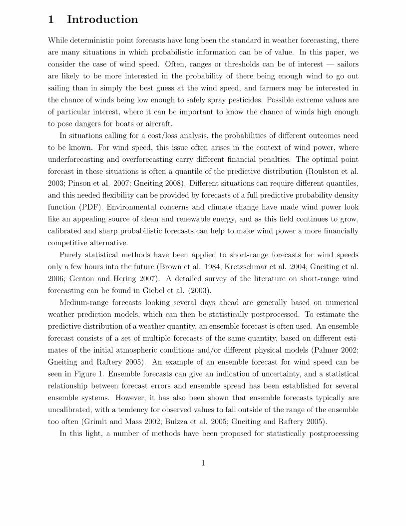
Gneiting and Raftery 2005). An example of an ensemble forecast for wind speed can be

seen in Figure 1. Ensemble forecasts can give an indication of uncertainty, and a statistical

relationship between forecast errors and ensemble spread has been established for several

ensemble systems. However, it has also been shown that ensemble forecasts typically are

uncalibrated, with a tendency for observed values to fall outside of the range of the ensemble

too often (Grimit and Mass 2002; Buizza et al. 2005; Gneiting and Raftery 2005).

In this light, a number of methods have been proposed for statistically postprocessing

1

Figure 1: 48-hour ahead ensemble forecast of maximum wind speed over the Pacific North-west on 7 August 2003 using the eight-member University of Washington mesoscale ensemble(Grimit and Mass 2002; Eckel and Mass 2005).

ensemble forecasts of wind speed or wind power. These approaches have largely focused on

the use of quantile regression to generate forecast bounds and/or intervals (Bremnes 2004;

Nielsen et al. 2006; Pinson et al. 2007; Møller et al. 2008). These methods do not, however,

yield a full PDF; rather, they give only probabilities for certain specific events.

Bayesian model averaging (BMA) was introduced by Raftery et al. (2005) as a statistical

postprocessing method for producing probabilistic forecasts from ensembles in the form of

predictive PDFs. The BMA predictive PDF of any future weather quantity of interest is

a weighted average of PDFs centered on the individual bias-corrected forecasts, where the

weights can be interpreted as posterior probabilities of the models generating the forecasts

and reflect the forecasts’ contributions to overall forecasting skill over a training period. The

original development of BMA by Raftery et al. (2005) was for weather quantities whose

predictive PDFs are approximately normal, such as temperature and sea-level pressure.

This method was modified by Sloughter et al. (2007) to apply to quantitative precipitation

forecasts. These forecasts used component distributions that had a positive probability of

being equal to zero, and, when not zero, were skewed, and modeled using power-transformed

gamma distributions.

As with precipitation, wind speed has a skewed distribution. Unlike for precipitation,

2

there is no need to model the separate probability of wind speed being equal to zero, at least

in the geographic region we consider. Here we develop a BMA method for wind speed by

modeling the component distribution for a given ensemble member as a gamma distribution;

the BMA PDF is then itself a mixture of such distributions.

In Section 2 we review the BMA technique and describe our extension of it to wind

speed. Statistical approaches to wind forecasting offer a unique challenge in that observed

values are reported discretized to the nearest whole knot, a much coarser discretization than

is seen in other weather quantities. We compare a number of methods for estimating the

parameters of the BMA PDF which account for the discretization in different ways. Then in

Section 3 we give results for 48-hour ahead forecasts of maximum wind speed over the North

American Pacific Northwest in 2003 based on the eight-member University of Washington

mesoscale ensemble (Grimit and Mass 2002; Eckel and Mass 2005). Throughout the paper

we use illustrative examples drawn from these data, and we find that BMA is calibrated and

sharp for the period we consider. Finally, in Section 4 we discuss alternative approaches and

possible improvements to the method.

2 Data and Methods

2.1 Forecast and observation data

This research considers 48-hour ahead forecasts of maximum wind speed over the Pacific

Northwest in the period from 1 November 2002 through 31 December 2003, using the eight-

member University of Washington mesoscale ensemble (Eckel and Mass 2005) initialized at

00 hours UTC, which is 5pm local time in summer, when daylight saving time operates,

and 4pm local time otherwise. The dataset contains observations and forecasts at surface

airway observation (SAO) stations, a network of automated weather stations located at

airports throughout the United States and Canada. Maximum wind speed is defined as

the maximum of the hourly ‘instantaneous’ wind speeds over the previous eighteen hours,

where an hourly ‘instantaneous’ wind speed is a 2-minute average from the period of two

minutes before the hour to on the hour. Data were available for 340 days, and data for

86 days during this period were unavailable. In all, 35,230 station observations were used,

an average of about 104 per day. The forecasts were produced for observation locations

by bilinear interpolation from forecasts generated on a twelve kilometer grid, as is common

practice in the meteorological community. The wind speed observations were subject to the

quality control procedures described by Baars (2005).

The wind speed data we analyze are discretized when recorded — wind speed is rounded

to the nearest whole knot. Additionally, any wind speeds below one knot are recorded as

3

zero. One knot is equal to approximately 0.514 meters per second, or 1.151 miles per hour.

2.2 Bayesian model averaging

Bayesian model averaging (BMA) (Leamer 1978; Kass and Raftery 1995; Hoeting et al.

1999) was originally developed as a way to combine inferences and predictions from multiple

statistical models, and was applied to statistical linear regression and related models in the

social and health sciences. Raftery et al. (2005) extended BMA to ensembles of deterministic

prediction models and showed how it can be used as a statistical postprocessing method

for forecast ensembles, yielding calibrated and sharp predictive PDFs of future weather

quantities.

In BMA for forecast ensembles, each ensemble member forecast fk is associated with a

component PDF, gk(y|fk). The BMA predictive PDF for the future weather quantity, y, is

then a mixture of the component PDFs, namely

p(y|f1, . . . , fK) =K∑

k=1

wk gk(y|fk), (1)

where the BMA weight wk is based on forecast k’s relative performance in the training

period. The wk’s are probabilities and so they are nonnegative and add up to 1, that is,∑Kk=1 wk = 1. Here K is the number of ensemble members.

The component PDF gk(y|fk) can be thought of roughly as the conditional PDF of the

weather quantity y given the kth forecast, fk, conditional on fk being the best forecast in the

ensemble. This heuristic interpretation is in line with how operational weather forecasters

often work, by selecting one or a small number of ‘best’ forecasts from a potentially large

number available, based on recent predictive performance (Joslyn and Jones 2008).

2.3 Gamma model

For weather variables such as temperature and sea level pressure, the component PDFs can

be fit reasonably well using a normal distribution centered at a bias-corrected forecast, as

shown by Raftery et al. (2005). For precipitation, Sloughter et al. (2007) modeled the

component PDFs using a mixture of a point mass at zero and a power-transformed gamma

distribution.

Haslett and Raftery (1989) modeled the square root of wind speeds using a normal distri-

bution. Wind speed distributions have also often been modeled by Weibull densities (Justus

et al. 1976; Hennessey 1977; Justus et al. 1978; Stevens and Smulders 1979). Tuller and

Brett (1984) noted that the necessary assumptions for fitting a Weibull distribution are not

always met. Here we generalize the Weibull approach by considering gamma distribution fits

4

to power transformations of the observed wind speeds. We found that gamma distributions

for the raw observed wind speeds gave a good fit, and fit better than using any power trans-

formation. In light of this, we model the component PDFs of wind speed as untransformed

gamma distributions. The gamma distribution with shape parameter α and scale parameter

β has the PDF

g(y) =1

βα Γ(α)yα−1 exp(−y/β) (2)

for y > 0, and g(y) = 0 for y ≤ 0. The mean of this distribution is µ = αβ, and its variance

is σ2 = αβ2.

It remains to specify how the parameters of the gamma distribution depend on the

numerical forecast. An exploratory data analysis showed that the observed wind speed is

approximately linear as a function of the forecasted wind speed, with a standard deviation

that is also approximately linear as a function of the forecast.

Putting these observations together, we get the following model for the component gamma

PDF of wind speed:

gk(y|fk) =1

βαk

k Γ(αk)yαk−1 exp(−y/βk). (3)

The parameters of the gamma distribution depend on the ensemble member forecast, fk,

through the relationships

µk = b0k + b1kfk, (4)

and

σk = c0k + c1kfk, (5)

where µk = αkβk is the mean of the distribution, and σk =√

αkβk is its standard devia-

tion. Here we restrict the standard deviation parameters to be constant across all ensemble

members. This simplifies the model by reducing the number of parameters to be estimated,

makes parameter estimation computationally easier, and reduces the risk of overfitting, and

we found that it led to no degradation in predictive performance. The c0k and c1k terms are

replaced with c0 and c1.

Our final BMA model for the predictive PDF of the weather quantity, y, here the maxi-

mum wind speed, is thus (1) with gk as defined in (3).

2.4 Parameter estimation

Parameter estimation is based on forecast-observation pairs from a training period, which

we take here to be the N most recent available days preceding initialization. The training

period is a sliding window, and the parameters are reestimated for each new initialization

period. We considered training periods ranging from the past 20 to 45 days. An examination

5

of the sensitivity of our results to training period length showed very similar performance

across potential training period lengths. Differences in average errors were only seen three

decimal places out. Within this range, we consistently saw that a 25 day training period

gave very slightly better performance, and we will present results here based on this period.

2.4.1 Standard method

We first consider a standard method of parameter estimation similar to the method used for

quantitative precipitation in Sloughter et al. (2007). We estimate the mean parameters, b0k

and b1k, by linear regression. These parameters are member-specific, and are thus estimated

separately for each ensemble member, using the observed wind speed as the dependent

variable and the forecasted wind speed, fk, as the independent variable.

We estimate the remaining parameters, w1, . . . , wK, c0, and c1, by maximum likelihood

from the training data. Assuming independence of forecast errors in space and time, the

log-likelihood function for the BMA model is

ℓ(w1, . . . , wK ; c0; c1) =∑s,t

log p(yst|f1st, . . . , fKst), (6)

where the sum extends over all station locations, s, and times, t, in the training data.

As noted above, wind speed observations below one knot are recorded as zero knots. The

log-likelihood requires calculating the logarithm of each observed wind speed, which is not

possible with values of zero.

Wilks (1990) suggested a method for maximum likelihood estimation of gamma distri-

bution parameters with data containing zeroes due to rounding by, for each value of zero,

replacing the corresponding component of the log-likelihood with the aggregated probability

of the range of values that would be rounded to zero (in our case, between 0 and 1 knots).

To incorporate this, for each observed yst recorded as a zero, we replace p(yst|f1st, . . . , fKst)

above with

p(yst|f1st, . . . , fKst) = P (1|f1st, . . . , fKst), (7)

where

P (a|f1st, . . . , fKst) =∫ a

0p(y|f1st, . . . , fKst) dy. (8)

The log-likelihood function cannot be maximized analytically, and instead we maximize

it numerically using the EM algorithm (Dempster et al. 1977; McLachlan and Krishnan

1997). The EM algorithm is iterative, and alternates between two steps, the expectation

(E) step, and the maximization (M) step. It uses the unobserved quantities zkst, which are

latent variables equal to 1 if observation yst comes from the kth mixture component, and to

0 otherwise.

6

In the E step, the zkst are estimated given the current estimate of the parameters. Specif-

ically,

z(j+1)kst =

w(j)k p(j)(yst|fkst)∑K

l=1 w(j)l p(j)(yst|flst)

, (9)

where the superscript j refers to the jth iteration of the EM algorithm, and thus w(j)k refers

to the estimate of wk at the jth iteration. The quantity p(j)(yst|fkst) is defined using the

estimates of c0 and c1 from the jth iteration, and is either gk(yst|fkst) as defined in (3), if yst

is non-zero, or is Gk(1|fkst), if yst is zero, where

Gk(a|fkst) =∫ a

0gk(y|fkst) dy. (10)

Note that, although the zkst are equal to either 0 or 1, the zkst are real numbers between 0

and 1. The z1st, . . . , zKst are nonnegative and sum to 1 for each (s, t).

The M step then consists of maximizing the expected log-likelihood as a function of

w1, . . . , wK , c0, and c1, where the expectation is taken over the distribution of zkst given the

data and the previous estimates. This is the same as maximizing the log-likelihood given

the zkst as well as w1, . . . , wK , c0, and c1, evaluated at zkst = z(j+1)kst . Thus

w(j+1)k =

1

n

∑s,t

z(j+1)kst , (11)

where n is the number of cases in the training set, that is, the number of distinct values of

(s, t). There are no analytic solutions for the M step estimates of the parameters c0 and c1,

and so they must be found numerically.

The E and M steps are then iterated to convergence, which we define as a change no

greater than some small tolerance in the log-likelihood in one iteration. The log-likelihood

is guaranteed to increase at each EM iteration (Wu 1983), which implies that in general it

converges to a local maximum of the likelihood. Convergence to a global maximum cannot be

guaranteed, so the solution reached by the algorithm can be sensitive to the starting values.

Choosing the starting values based on equal weights and the marginal variance usually led

to a good solution in our experience.

2.4.2 Fully discretized method

While our standard method addresses the computational issues associated with recorded

observations of zero, it does not more generally address the discretization of the wind speed

values. We therefore consider a fully discretized method of parameter estimation that gener-

alizes the method of Wilks (1990). Each component of the log-likelihood is replaced with the

aggregated probability of the range of values that would be rounded to the recorded value.

7

In our case, a recorded observation of 0 indicates a true value between 0 and 1, a recorded

observation of 1 indicates a true value between 1 and 32, and for any integer i > 1, a recorded

observation of i indicates a true value between i − 12

and i + 12.

To extend the approach of our initial method, we first leave p(yst|f1st, . . . , fKst) as defined

in (7) for observed values of 0. For observed values of 1, we have

p(yst|f1st, . . . , fKst) = P (32|f1st, . . . , fKst) − P (1|f1st, . . . , fKst), (12)

and for observed values i where i > 1,

p(yst|f1st, . . . , fKst) = P (i + 12|f1st, . . . , fKst) − P (i− 1

2|f1st, . . . , fKst). (13)

Analogously, in the E step of the EM algorithm, for observed values of 0, we put

p(j)(yst|fkst) = Gk(1|fkst), (14)

for observed values of 1,

p(j)(yst|fkst) = Gk(32|fkst) − Gk(1|fkst), (15)

and for observed values i where i > 1,

p(j)(yst|fkst) = Gk(i + 12|fkst) − Gk(i − 1

2|fkst). (16)

The rest of the EM algorithm remains unchanged.

2.4.3 Doubly discretized method

In the fully discretized method, the discretization of observations is taken into account in

the log-likelihood. This allows us to account for the discretization when estimating the

BMA weights and the standard deviation parameters, which are estimated via maximum

likelihood. However, this does not address the mean parameters, which are fit via linear

regression. To take account of the discretization in estimating the mean parameters, we

additionally discretize the forecasts in the same manner that the observations have been.

The parameters are then estimated as in the fully discretized method, replacing the ensemble

member forecasts with the discretized forecasts.

2.4.4 Pure maximum likelihood method

We next investigate the possibility of estimating the mean parameters by maximum likelihood

as well. To avoid computational problems with a parameter space of too high a dimension,

we restrict the mean parameters to be constant across ensemble members, similarly to the

8

constraint already placed on the standard deviation parameters. We then estimate the BMA

weights, mean parameters, and standard deviation parameters simultaneously via maximum

likelihood, using the discretized log-likelihood function from the fully discretized method.

The log-likelihood is optimized numerically.

2.4.5 Parsimonious method

We finally consider one additional method, taking the partially discretized log-likelihood

from the standard method but adding the constraint that the mean parameters must be

constant across ensemble members. This represents the most parsimonious model, in that it

has the smallest number of parameters.

3 Results

We begin by looking at aggregate results over the entire Pacific Northwest domain, for the

full 2003 calendar year, with the data available from late 2002 used only as training data,

to allow us to create forecasts starting in January. The following section will then look at

some more specific examples of results for individual locations and/or times.

3.1 Results for the Pacific Northwest

In assessing probabilistic forecasts of wind speed, we aim to maximize the sharpness of the

predictive PDFs subject to calibration (Gneiting, Balabdaoui, and Raftery 2007). Calibra-

tion refers to the statistical consistency between the forecast PDFs and the observations.

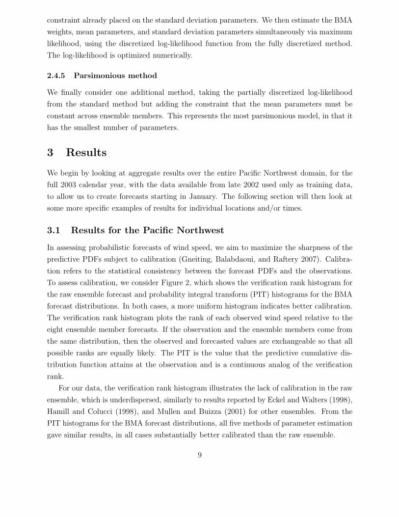
To assess calibration, we consider Figure 2, which shows the verification rank histogram for

the raw ensemble forecast and probability integral transform (PIT) histograms for the BMA

forecast distributions. In both cases, a more uniform histogram indicates better calibration.

The verification rank histogram plots the rank of each observed wind speed relative to the

eight ensemble member forecasts. If the observation and the ensemble members come from

the same distribution, then the observed and forecasted values are exchangeable so that all

possible ranks are equally likely. The PIT is the value that the predictive cumulative dis-

tribution function attains at the observation and is a continuous analog of the verification

rank.

For our data, the verification rank histogram illustrates the lack of calibration in the raw

ensemble, which is underdispersed, similarly to results reported by Eckel and Walters (1998),

Hamill and Colucci (1998), and Mullen and Buizza (2001) for other ensembles. From the

PIT histograms for the BMA forecast distributions, all five methods of parameter estimation

gave similar results, in all cases substantially better calibrated than the raw ensemble.

9

(a) (b) (c)

(d) (e) (f)

Figure 2: Calibration checks for probabilistic forecasts of wind speed over the Pacific North-west in 2003. (a) Verification rank histogram for the raw ensemble, and PIT histogramsfor the BMA forecast distributions estimated using (b) the standard method, (c) the fullydiscretized method, (d) the doubly discretized method, (e) the pure maximum likelihoodmethod, and (f) the parsimonious method.

If the eight-member raw ensemble were properly calibrated, there would bea 19

probability

of the wind speed observation falling below the ensemble range, and a 19

probability of it

falling above the ensemble range. As such, to allow direct comparisons to the raw ensemble,

we will consider 79

or 77.8% central prediction intervals from the BMA PDF. Table 1 shows

the empirical coverage of 77.8% prediction intervals, and the results echo what we see in

the verification rank and PIT histograms. The raw ensemble was highly uncalibrated. The

BMA intervals were well calibrated. The table also shows the average width of the prediction

intervals, which characterizes the sharpness of the forecast distributions. While the raw

ensemble provides a narrower interval, this comes at the cost of much poorer calibration.

Scoring rules provide summary measures of predictive performance that address calibra-

tion and sharpness simultaneously. A particularly attractive scoring rule for probabilistic

forecasts of a scalar variable is the continuous ranked probability score (CRPS), which gen-

10

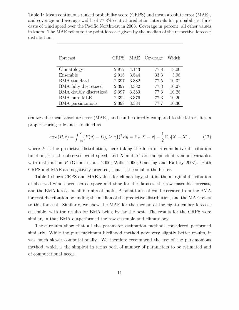
Table 1: Mean continuous ranked probability score (CRPS) and mean absolute error (MAE),and coverage and average width of 77.8% central prediction intervals for probabilistic fore-casts of wind speed over the Pacific Northwest in 2003. Coverage in percent, all other valuesin knots. The MAE refers to the point forecast given by the median of the respective forecastdistribution.

Forecast CRPS MAE Coverage Width

Climatology 2.972 4.143 77.8 13.00Ensemble 2.918 3.544 33.3 3.98BMA standard 2.397 3.382 77.5 10.32BMA fully discretized 2.397 3.382 77.3 10.27BMA doubly discretized 2.397 3.383 77.3 10.28BMA pure MLE 2.392 3.376 77.3 10.20BMA parsimonious 2.398 3.384 77.7 10.36

eralizes the mean absolute error (MAE), and can be directly compared to the latter. It is a

proper scoring rule and is defined as

crps(P, x) =∫

∞

−∞

(P (y) − I{y ≥ x})2 dy = EP |X − x| − 1

2EP |X − X ′|, (17)

where P is the predictive distribution, here taking the form of a cumulative distribution

function, x is the observed wind speed, and X and X ′ are independent random variables

with distribution P (Grimit et al. 2006; Wilks 2006; Gneiting and Raftery 2007). Both

CRPS and MAE are negatively oriented, that is, the smaller the better.

Table 1 shows CRPS and MAE values for climatology, that is, the marginal distribution

of observed wind speed across space and time for the dataset, the raw ensemble forecast,

and the BMA forecasts, all in units of knots. A point forecast can be created from the BMA

forecast distribution by finding the median of the predictive distribution, and the MAE refers

to this forecast. Similarly, we show the MAE for the median of the eight-member forecast

ensemble, with the results for BMA being by far the best. The results for the CRPS were

similar, in that BMA outperformed the raw ensemble and climatology.

These results show that all the parameter estimation methods considered performed

similarly. While the pure maximum likelihood method gave very slightly better results, it

was much slower computationally. We therefore recommend the use of the parsimonious

method, which is the simplest in terms both of number of parameters to be estimated and

of computational needs.

11

0 5 10 15 20 25

0.00

0.05

0.10

0.15

0.20

Wind speed in knots

Den

sity

Figure 3: 48-hour ahead BMA predictive PDF for maximum wind speed at Shelton, Wash-ington on 7 August 2003. The upper solid curve is the BMA PDF. The lower curves are thecomponents of the BMA PDF, namely, the weighted contributions from the ensemble mem-bers. The dashed vertical lines represent the 11th and 89th percentiles of the BMA PDF; thedashed horizontal line is the respective prediction interval; the circles represent the ensemblemember forecasts; and the solid vertical line represents the verifying observation.

3.2 Examples

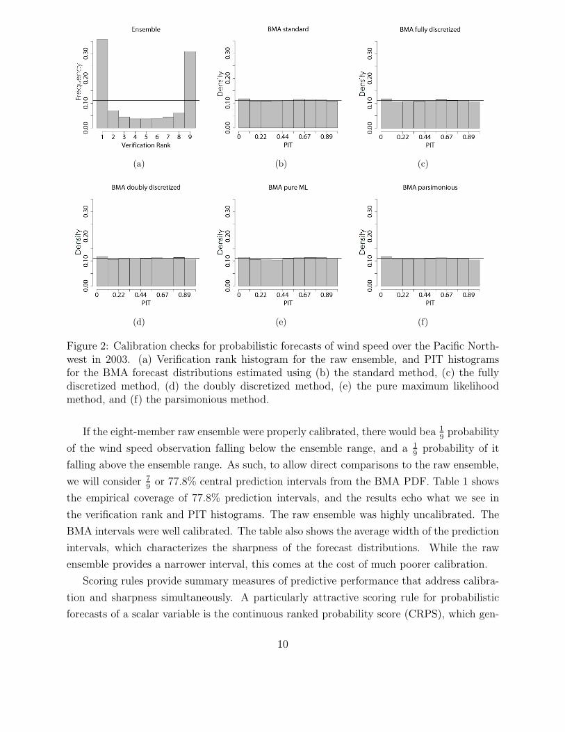
To illustrate the BMA forecast distributions for wind speed, we show an example, on 7 August

2003 at Shelton, Washington. Figure 3 shows the ensemble values, the BMA component

distributions, the BMA PDF, the BMA central 77.8% forecast interval, and the observation.

The observed wind speed of 12 knots fell just above the ensemble range, while it was within

the range of the BMA interval.

Figure 4 shows maps of the BMA median and BMA 90th percentile upper bound forecast

for 7 August 2003. If we compare to the ensemble forecast in Figure 1 we see that the general

spatial structure is largely preserved in the BMA forecast. Figure 5 shows the verifying wind

observations over the Pacific Northwest on 7 August 2003. It is evident that the raw ensemble

was underforecasting in a number of areas where the BMA forecast was not.

Finally, we compare the BMA forecasts at Shelton, Washington over the 2003 calendar

year to the raw ensemble forecast and the station climatology, that is, the marginal dis-

tribution of all observed values at Shelton over the time period considered. Table 2 shows

CRPS and MAE scores along with prediction interval coverage and average width for sta-

tion climatology, the raw ensemble, and BMA at this location. The BMA forecast showed

12

(a) (b)

Figure 4: 48-hour ahead (a) BMA median forecast, and (b) BMA 90th percentile forecast ofmaximum wind speed over the Pacific Northwest on 7 August 2003.

Figure 5: Observed maximum wind speeds at meteorological stations over the Pacific North-west on 7 August 2003. The arrow indicates the station at Shelton, Washington.

13

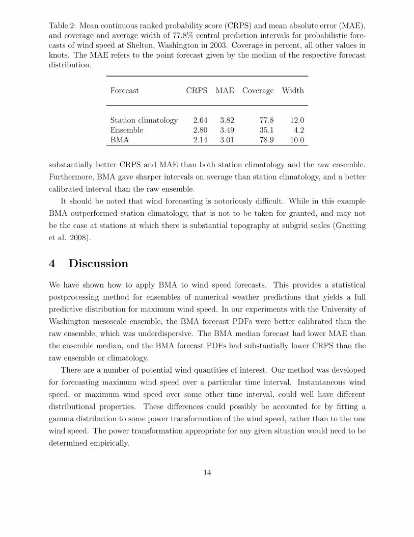
Table 2: Mean continuous ranked probability score (CRPS) and mean absolute error (MAE),and coverage and average width of 77.8% central prediction intervals for probabilistic fore-casts of wind speed at Shelton, Washington in 2003. Coverage in percent, all other values inknots. The MAE refers to the point forecast given by the median of the respective forecastdistribution.

Forecast CRPS MAE Coverage Width

Station climatology 2.64 3.82 77.8 12.0Ensemble 2.80 3.49 35.1 4.2BMA 2.14 3.01 78.9 10.0

substantially better CRPS and MAE than both station climatology and the raw ensemble.

Furthermore, BMA gave sharper intervals on average than station climatology, and a better

calibrated interval than the raw ensemble.

It should be noted that wind forecasting is notoriously difficult. While in this example

BMA outperformed station climatology, that is not to be taken for granted, and may not

be the case at stations at which there is substantial topography at subgrid scales (Gneiting

et al. 2008).

4 Discussion

We have shown how to apply BMA to wind speed forecasts. This provides a statistical

postprocessing method for ensembles of numerical weather predictions that yields a full

predictive distribution for maximum wind speed. In our experiments with the University of

Washington mesoscale ensemble, the BMA forecast PDFs were better calibrated than the

raw ensemble, which was underdispersive. The BMA median forecast had lower MAE than

the ensemble median, and the BMA forecast PDFs had substantially lower CRPS than the

raw ensemble or climatology.

There are a number of potential wind quantities of interest. Our method was developed

for forecasting maximum wind speed over a particular time interval. Instantaneous wind

speed, or maximum wind speed over some other time interval, could well have different

distributional properties. These differences could possibly be accounted for by fitting a

gamma distribution to some power transformation of the wind speed, rather than to the raw

wind speed. The power transformation appropriate for any given situation would need to be

determined empirically.

14

Nielsen et al. (2004) presented a probabilistic forecasting method based on correcting

quantiles of an ensemble, while other approaches have used climatology conditioned on en-

semble forecasts (Roulston et al. 2003) or on numerical weather prediction model output

(Bremnes 2006). The model based approach of BMA allows for the fitting of a predictive

distribution using sparse training data. By modeling the relation between forecasts and ob-

servations, BMA allows for the creation of forecast distributions in situations where the raw

forecasts may not have any close analogues in the training set.

Our results showed no appreciable difference in performance between parameter estima-

tion methods that took into account the discretization of the data and those that did not. A

detailed simulation study looking at the effects of discretization for meteorological data was

carried out by Cooley et al. (2007). Perrin et al. (2006) found that discretized wind speed

values can result in erroneously low standard errors for parameter estimates. However, we do

not look at standard errors of our parameter estimates here, as we are interested primarily

in prediction, and not in parameter estimation for its own sake.

While our implementation has been for a situation where the ensemble members come

from clearly distinguishable sources, it is easily modifiable to deal with situations in which

ensemble members come from the same model, differing only in some random perturbations,

such as the global ensembles that are currently used by the National Centers for Environ-

mental Prediction and the European Centre for Medium-Range Weather Forecasts (Buizza

et al. 2005). In these cases, members coming from the same source should be treated as

exchangeable, and thus should have equal weight and equal BMA parameter values across

members. As our recommended parsimonious method already constrains the mean and stan-

dard deviation parameters to be equal across all members, the only change that would need

to be made would be to add the constraint that the BMA weights be equal, as described by

Raftery et al. (2005, p. 1170) and Wilson et al. (2007).

Our approach has not incorporated temporal autocorrelation. While wind speeds in suc-

cessive time periods are certainly autocorrelated, our method implicitly addresses forecast

errors rather than raw wind speeds, because it models the predictive distribution conditional

on the numerical forecasts. Exploratory work has shown that there is little or no autocor-

relation in forecast errors of wind speeds, so the numerical forecasts effectively take care of

the autocorrelation in the wind speeds themselves. To incorporate temporal autocorrelation,

the method would have to be made considerably more complicated, and it seems unlikely

that this would improve its predictive performance appreciably.

Our method produces wind speed forecasts at individual locations, which is the focus

of many, and possibly most applications. As a result we have not had to model spatial

correlation between wind speeds, although these definitely are present. In applications that

15

involve forecasting wind speeds at more than one location simultaneously, it would be vital

to take account of spatial correlation. These include forecasting maximum wind speeds

over an area or trajectory, for example for shipping or boating, and forecasting the total

energy from several wind farms in a region. Methods for probabilistic weather forecasting at

multiple locations simultaneously have been developed for temperature (Gel, Raftery, and

Gneiting 2004; Berrocal, Raftery, and Gneiting 2007), for precipitation (Berrocal, Raftery,

and Gneiting 2009), and for temperature and precipitation simultaneously (Berrocal et al.

2007). These methods could possibly be extended to wind speeds.

Our method estimates a single set of parameters across the entire domain. Nott et al.

(2001) noted that localized statistical postprocessing can address issues of locally varying

biases in numerical weather forecasts. A localized version of BMA for temperature, based

on taking sets of forecasts and observations within a carefully selected neighborhood, has

shown substantial improvements over the global version (Mass et al. 2008), and it is likely

that similar improvements would be seen for a localized version of BMA for wind speed.

Either the global or localized parameter estimation can be used to create probabilistic

forecasts of wind speed on a spatial grid. These methods have already been implemented for

temperature and precipitation and provide real-time probabilistic weather forecasts over

the Pacific Northwest (Mass et al. 2008), which are available to the general public at

http://probcast.washington.edu. We intend to make similar, gridded probabilistic fore-

casts for wind speed available also. Additionally, for specialized uses where only a single

location is of interest, such as a wind farm or a windsurfing or sailing location, BMA param-

eters could be fit using the same methodology as described in this paper, but restricting it

to use only data from that particular location.

References

Baars, J. (2005). Observations QC summary page — http://www.atmos.washington.edu/

mm5rt/qc obs/qc obs stats.html.

Berrocal, V. J., A. E. Raftery, and T. Gneiting (2007). Combining spatial statistical and

ensemble information in probabilistic weather forecasts. Monthly Weather Review 135,

1306–1402.

Berrocal, V. J., A. E. Raftery, and T. Gneiting (2009). Probabilistic quantitative precip-

itation forecasting using a two-stage spatial model. Annals of Applied Statistics, to

appear.

Berrocal, V. J., A. E. Raftery, T. Gneiting, and R. C. Steed (2007). Probabilistic

16

weather forecasting for winter road maintenance. Technical Report 511, Department of

Statistics, University of Washington, Seattle, Wash. Available at http://www.stat.

washington.edu/research/reports/.

Bremnes, J. B. (2004). Probabilistic wind power forecasts using local quantile regression.

Wind Energy 7, 47–54.

Bremnes, J. B. (2006). A comparison of a few statistical models for making quantile wind

power forecasts. Wind Energy 9, 3–11.

Brown, B. G., R. W. Katz, and A. H. Murphy (1984). Time series models to simulate and

forecast wind speed and wind power. Journal of Climate and Applied Meteorology 23,

1184–1195.

Buizza, R., P. L. Houtekamer, Z. Toth, G. Pellerin, M. Wei, and Y. Zhu (2005). A com-

parison of the ECMWF, MSC and NCEP global ensemble prediction systems. Monthly

Weather Review 133, 1076–1097.

Cooley, D., D. Nychka, and P. Naveau (2007). Bayesian spatial modeling of extreme

precipitation return levels. Journal of the American Statistical Association 102, 824–

840.

Dempster, A. P., N. M. Laird, and D. B. Rubin (1977). Maximum likelihood from incom-

plete data via the EM algorithm. Journal of the Royal Statistical Society Series B 39,

1–39.

Eckel, F. and M. Walters (1998). Calibrated probabilistic quantitative precipitation fore-

casts based on the MRF ensemble. Weather and Forecasting 13, 1132–1147.

Eckel, F. A. and C. F. Mass (2005). Effective mesoscale, short-range ensemble forecasting.

Weather and Forecasting 20, 328–350.

Gel, Y., A. E. Raftery, and T. Gneiting (2004). Calibrated probabilistic mesoscale weather

field forecasting: The geostatistical output perturbation (GOP) method (with discus-

sion). Journal of the American Statistical Association 99, 575–590.

Genton, M. and A. Hering (2007). Blowing in the wind. Significance 4, 11–14.

Giebel, G., R. Brownsword, and G. Kariniotakis (2003). The state-of-the-art in short-

term prediction of wind power. Deliverable Report D1.1, Project Anemos, available at

http://anemos.cma.fr/download/ANEMOS D1.1 StateOfTheArt v1.1.pdf.

Gneiting, T. (2008). Quantiles as optimal point predictors. Technical Report 538, De-

partment of Statistics, University of Washington. Available at http://www.stat.

washington.edu/research/reports/.

17

Gneiting, T., F. Balabdaoui, and A. E. Raftery (2007). Probabilistic forecasts, calibration

and sharpness. Journal of the Royal Statistical Society Series B 69, 243–268.

Gneiting, T., K. Larson, K. Westrick, M. G. Genton, and E. Aldrich (2006). Calibrated

probabilistic forecasting at the Stateline wind energy center: The regime-switching

space-time method. Journal of the American Statistical Association 101, 968–979.

Gneiting, T. and A. E. Raftery (2005). Weather forecasting with ensemble methods. Sci-

ence 310, 248–249.

Gneiting, T. and A. E. Raftery (2007). Strictly proper scoring rules, prediction, and

estimation. Journal of the American Statistical Association 102, 359–378.

Gneiting, T., L. I. Stanberry, E. P. Grimit, L. Held, and N. A. Johnson (2008). Assess-

ing probabilistic forecasts of multivariate quantities, with applications to ensemble

predictions of surface winds (with discussion and rejoinder). Test 17, 211–264.

Grimit, E. P., T. Gneiting, V. J. Berrocal, and N. A. Johnson (2006). The continuous

ranked probability score for circular variables and its application to mesoscale forecast

ensemble verification. Quarterly Journal of the Royal Meteorological Society 132, 3209–

3220.

Grimit, E. P. and C. F. Mass (2002). Initial results of a mesoscale short-range ensemble

forecasting system over the Pacific Northwest. Weather and Forecasting 17, 192–205.

Hamill, T. M. and S. J. Colucci (1998). Evaluation of Eta-RSM ensemble probabilistic

precipitation forecasts. Monthly Weather Review 126, 711–724.

Haslett, J. and A. E. Raftery (1989). Space-time modelling with long-memory depen-

dence: Assessing Ireland’s wind power resource (with discussion). Journal of the Royal

Statistical Society Series C: Applied Statistics 38, 1–50.

Hennessey, J. P. J. (1977). Some aspects of wind power statistics. Journal of Applied

Meteorology 16, 119–128.

Hoeting, J. A., D. M. Madigan, A. E. Raftery, and C. T. Volinsky (1999). Bayesian model

averaging: A tutorial (with discussion). Statistical Science 14, 382–401. A corrected

version with typos corrected is available at http://www.stat.washington.edu/www/

research/online/hoeting1999.pdf.

Joslyn, S. and D. W. Jones (2008). Strategies in naturalistic decision-making: A cognitive

task analysis of naval weather forecasting. In J. M. Schraagen, L. Militello, T. Ormerod,

and R. Lipshitz (Eds.), Naturalistic Decision Making and Macrocognition, pp. 183–202.

Aldershot, U.K.: Ashgate Publishing.

18

Justus, C. G., W. R. Hargraves, A. Mikhail, and D. Graber (1978). Methods for estimating

wind speed frequency distributions. Journal of Applied Meteorology 17, 350–353.

Justus, C. G., W. R. Hargraves, and A. Yalcin (1976). Nationwide assessment of potential

output from wind-powered generators. Journal of Applied Meteorology 15, 673–678.

Kass, R. E. and A. E. Raftery (1995). Bayes factors. Journal of the American Statistical

Association 90, 773–795.

Kretzschmar, R., P. Eckert, D. Cattani, and F. Eggimann (2004). Neural network classi-

fiers for local wind prediction. Journal of Applied Meteorology 43, 727–738.

Leamer, E. E. (1978). Specification Searches. New York: Wiley.

Mass, C., S. Joslyn, J. Pyle, P. Tewson, T. Gneiting, A. Raftery, J. Baars, J. M. Sloughter,

D. Jones, and C. Fraley (2008). PROBCAST: A web-based portal to mesoscale prob-

abilistic forecasts. Submitted to Bulletin of the American Meteorological Society .

McLachlan, G. J. and T. Krishnan (1997). The EM Algorithm and Extensions. New York:

Wiley.

Møller, J. K., H. A. Nielsen, and H. Madsen (2008). Time-adaptive quantile regression.

Computational Statistics & Data Analysis 52, 1292–1303.

Mullen, S. L. and R. Buizza (2001). Quantitative precipitation forecasts over the United

States by the ECMWF ensemble prediction system. Monthly Weather Review 129,

638–663.

Nielsen, H. A., H. Madsen, and T. S. Nielsen (2006). Using quantile regression to extend

an existing wind power forecasting system with probabilistic forecasts. Wind Energy 9,

95–108.

Nielsen, H. A., H. Madsen, T. S. Nielsen, J. Badger, G. Giebel, L. Landberg, K. Sattler,

and H. Feddersen (2004). Wind power ensemble forecasting. In Proceedings of the 2004

Global Windpower Conference and Exhibition, Chicago, Illinois, USA.

Nott, D. J., W. T. M. Dunsmuir, R. Kohn, and F. Woodcock (2001). Statistical correc-

tion of a deterministic numerical weather prediction model. Journal of the American

Statistical Association 96, 794–804.

Palmer, T. N. (2002). The economic value of ensemble forecasts as a tool for risk assess-

ment: From days to decades. Quarterly Journal of the Royal Meteorological Society 128,

747–774.

Perrin, O., H. Rootzen, and R. Taesler (2006). A discussion of statistical methods used to

estimate extreme wind speeds. Theoretical and Applied Climatology 85, 203–215.

19

Pinson, P., C. Chevallier, and G. N. Kariniotakis (2007). Trading wind generation with

short-term probabilistic forecasts of wind power. IEEE Transactions on Power Sys-

tems 22, 1148–1156.

Pinson, P., H. A. Nielsen, J. K. Møller, H. Madsen, and G. N. Kariniotakis (2007). Non-

parametric probabilistic forecasts of wind power: Required properties and evaluation.

Wind Energy 10, 497–516.

Raftery, A. E., T. Gneiting, F. Balabdaoui, and M. Polakowski (2005). Using Bayesian

model averaging to calibrate forecast ensembles. Monthly Weather Review 133, 1155–

1174.

Roulston, M. S., D. T. Kaplan, J. Hardenberg, and L. A. Smith (2003). Using medium-

range weather forcasts to improve the value of wind energy production. Renewable

Energy 28, 585–602.

Sloughter, J. M., A. E. Raftery, T. Gneiting, and C. Fraley (2007). Probabilistic quan-

titative precipitation forecasting using Bayesian model averaging. Monthly Weather

Review 135, 3209–3220.

Stevens, M. J. M. and P. T. Smulders (1979). The estimation of the parameters of the

Weibull wind speed distribution for wind energy utilization purposes. Wind Engineer-

ing 3, 132–145.

Tuller, S. E. and A. C. Brett (1984). The characteristics of wind velocity that favor the

fitting of a Weibull distribution in wind speed analysis. Journal of Applied Meteorol-

ogy 23, 124–134.

Wilks, D. S. (1990). Maximum likelihood estimation for the gamma distribution using

data containing zeros. Journal of Climate 3, 1495–1501.

Wilks, D. S. (2006). Statistical Methods in the Atmospheric Sciences (2nd ed.). Burlington:

Elsevier Academic Press.

Wilson, L. J., S. Beauregard, A. E. Raftery, and R. Verret (2007). Reply. Monthly Weather

Review 135, 4231–4236.

Wu, C. F. J. (1983). On the convergence properties of the EM algorithm. Annals of

Statistics 11, 95–103.

20