Probabilistic Methods in Combinatorial and

Stochastic Optimization

by

Jan Vondrak

Submitted to the Department of Mathematics

in partial fulfillment of the requirements for the degree of

Doctor of Philosophy

at the

MASSACHUSETTS INSTITUTE OF TECHNOLOGY

February 2005

c© Jan Vondrak, MMV. All rights reserved.

The author hereby grants to MIT permission to reproduce and

distribute publicly paper and electronic copies of this thesis documentin whole or in part.

Author . . . . . . . . . . . . . . . . . . . . . . . . . . . . . . . . . . . . . . . . . . . . . . . . . . . . . . . . . . . . . .Department of Mathematics

January 14, 2005

Certified by. . . . . . . . . . . . . . . . . . . . . . . . . . . . . . . . . . . . . . . . . . . . . . . . . . . . . . . . . .

Michel X. GoemansProfessor of Applied Mathematics

Thesis Supervisor

Accepted by . . . . . . . . . . . . . . . . . . . . . . . . . . . . . . . . . . . . . . . . . . . . . . . . . . . . . . . . .Rodolfo Ruben Rosales

Chairman, Applied Mathematics Committee

2

Probabilistic Methods in Combinatorial and StochasticOptimization

byJan Vondrak

Submitted to the Department of Mathematicson January 14, 2005, in partial fulfillment of the

requirements for the degree ofDoctor of Philosophy

Abstract

In this thesis we study a variety of combinatorial problems with inherent randomness.In the first part of the thesis, we study the possibility of covering the solutions of anoptimization problem on random subgraphs. The motivation for this approach is asituation where an optimization problem needs to be solved repeatedly for randominstances. Then we seek a pre-processing stage which would speed-up subsequentqueries by finding a fixed sparse subgraph covering the solution for a random subgraphwith high probability. The first problem that we investigate is the minimum spanningtree. Our essential result regarding this problem is that for every graph with edgeweights, there is a set of O(n log n) edges which contains the minimum spanning treeof a random subgraph with high probability. More generally, we extend this resultto matroids. Further, we consider optimization problems based on the shortest pathmetric and we find covering sets of size O(n1+2/c log2 n) that approximate the shortestpath metric of a random vertex-induced subgraph within a constant factor of c withhigh probability.

In the second part, we turn to a model of stochastic optimization, where a solu-tion is built sequentially by selecting a collection of “items”. We distinguish betweenadaptive and non-adaptive strategies, where adaptivity means being able to perceivethe precise characteristics of chosen items and use this knowledge in subsequent de-cisions. The benefit of adaptivity is our central concept which we investigate for avariety of specific problems. For the Stochastic Knapsack problem, we prove constantupper and lower bounds on the “adaptivity gap” between optimal adaptive and non-adaptive policies. For more general Stochastic Packing/Covering problems, we proveupper and lower bounds on the adaptivity gap depending on the dimension. We alsodesign polynomial-time algorithms achieving near-optimal approximation guaranteeswith respect to the adaptive optimum. Finally, we prove complexity-theoretic resultsregarding optimal adaptive policies. These results are based on a connection betweenadaptive policies and Arthur-Merlin games which yields PSPACE-hardness results fornumerous questions regarding adaptive policies.

Thesis Supervisor: Michel X. GoemansTitle: Professor of Applied Mathematics

3

4

Acknowledgments

First and foremost, my sincere thanks go to my advisor, Michel Goemans. His influ-ence permeates every part of this thesis, from informal discussions, invaluable sug-gestions and ideas, through brain-storming sessions in his office, to a never-endingchallenge to push the limits of my ability. My thanks go to Michel not only for be-ing my academic advisor but also for being a wise mentor and cheerful companionthroughout my years at MIT, never confining his support to the area of academics.Thanks for all the time you gave me, knowing how scarce your time can be!

I would also like to thank Santosh Vempala, for his inspiring classes, many helpfuldiscussions and motivating questions (which inspired especially Chapter 4 of thisthesis). My thanks go to many other professors at MIT, that I had the opportunityto work with or learn from. I would like to name especially Dan Kleitman, Igor Pak,Rom Pinchasi, Peter Shor, Mike Sipser, Dan Spielman, David Karger, Piotr Indyk,Arthur Mattuck and Hartley Rogers. Big thanks to Janos Pach at NYU, for recentcollaboration and generous support. Thanks to other collaborators, namely NicoleImmorlica, without whom the first half of my thesis would never get started, andBrian Dean, without whom the second half of my thesis would never get started,Rados Radoicic, whose merits go beyond being a collaborator, and finally Tim Chowand Kenneth Fan.

I should not forget to express my gratitude to those back home who made itpossible for me to come to MIT and who taught me many things that still helpmy brain tick. Foremost, my advisor in Prague, Martin Loebl, for all his support,unceasing mathematical curiosity and indomitable optimism. A lot of thanks to JirkaMatousek for his wonderful lectures and discussions. Thanks to both of you for yourbarely warranted belief in me. Thanks to Jaroslav Nesetril, Jan Kratochvıl and manyothers for creating an amazing academic environment at KAM MFF UK. And mydeepest gratitude to my parents in Prague, my brother Sipak, and the rest of thefamily, for being always there for me.

During my years at MIT, I met many friends who made my years in Boston greatfun and a wonderful experience. Thanks to Sergi for being my friend and colleaguein math from Day 1 in Boston. Thanks to Rados for his uplifting sarcasm, unyieldingcriticism and profound advice in many life situations. Thanks to Fumei for her smilingsupport in all these years. Thanks to all my friends in the department: Brad, Brian,Ian, Kevin, Jaheyuk, Boguk and Vahab. Best regards to old man Young Han. Manythanks to others who helped create the great atmosphere at MIT and who are nowscattered around the world: Jose, Mohammad, Kari, Wai Ling and others. Outside ofMIT, I would like to thank all the people who were my companions at times cheerfulor difficult: Rad, Yurika, David, Summer and Sun; Pavel, Alois, Jirka and Ying;Hazhir and Anya; Kalina and Samantha. Thanks to Martin for being a big friend,roommate and dangerous influence in the last two years.

And finally, thank you, Maryam, for making my last year of graduate school thehappiest one.

5

6

Contents

1 Introduction 91.1 Optimization problems on random subgraphs . . . . . . . . . . . . . . 91.2 Stochastic optimization and adaptivity . . . . . . . . . . . . . . . . . 12

2 Optimization problems on random subgraphs 172.1 The MST-covering problem . . . . . . . . . . . . . . . . . . . . . . . 182.2 The metric approximation problem . . . . . . . . . . . . . . . . . . . 192.3 Literature review . . . . . . . . . . . . . . . . . . . . . . . . . . . . . 20

2.3.1 MST covering . . . . . . . . . . . . . . . . . . . . . . . . . . . 202.3.2 Metric approximation . . . . . . . . . . . . . . . . . . . . . . . 20

3 Covering the minimum spanning tree of random subgraphs 233.1 The first attempt . . . . . . . . . . . . . . . . . . . . . . . . . . . . . 233.2 The boosting lemma . . . . . . . . . . . . . . . . . . . . . . . . . . . 253.3 Covering the MSTs of random vertex-induced subgraphs . . . . . . . 283.4 Improving the constant factor . . . . . . . . . . . . . . . . . . . . . . 293.5 Covering the MSTs of subgraphs of fixed size . . . . . . . . . . . . . . 303.6 Algorithmic construction of covering sets . . . . . . . . . . . . . . . . 323.7 Covering minimum-weight bases in matroids . . . . . . . . . . . . . . 343.8 Lower bounds . . . . . . . . . . . . . . . . . . . . . . . . . . . . . . . 37

4 Metric approximation for random subgraphs 414.1 Covering shortest paths . . . . . . . . . . . . . . . . . . . . . . . . . . 414.2 Approximating the shortest-path metric . . . . . . . . . . . . . . . . 434.3 Construction of metric-approximating sets for random vertex-induced

subgraphs . . . . . . . . . . . . . . . . . . . . . . . . . . . . . . . . . 434.4 Construction of metric-approximating sets for random edge-induced

subgraphs . . . . . . . . . . . . . . . . . . . . . . . . . . . . . . . . . 46

5 Stochastic Optimization and Adaptivity 475.1 Stochastic Knapsack . . . . . . . . . . . . . . . . . . . . . . . . . . . 485.2 Stochastic Packing and Covering problems . . . . . . . . . . . . . . . 505.3 Questions and gaps . . . . . . . . . . . . . . . . . . . . . . . . . . . . 535.4 Literature review . . . . . . . . . . . . . . . . . . . . . . . . . . . . . 55

5.4.1 Stochastic Optimization . . . . . . . . . . . . . . . . . . . . . 55

7

5.4.2 Stochastic Knapsack . . . . . . . . . . . . . . . . . . . . . . . 565.4.3 Stochastic Packing . . . . . . . . . . . . . . . . . . . . . . . . 575.4.4 Stochastic Covering . . . . . . . . . . . . . . . . . . . . . . . . 57

6 Stochastic Knapsack 596.1 Bounding adaptive policies . . . . . . . . . . . . . . . . . . . . . . . . 596.2 A 32/7-approximation for Stochastic Knapsack . . . . . . . . . . . . . 616.3 A stronger bound on adaptive policies . . . . . . . . . . . . . . . . . 646.4 A 4-approximation for Stochastic Knapsack . . . . . . . . . . . . . . 67

7 Stochastic Packing 717.1 Bounding adaptive policies . . . . . . . . . . . . . . . . . . . . . . . . 717.2 Stochastic Packing and hardness of PIP . . . . . . . . . . . . . . . . . 737.3 The benefit of adaptivity . . . . . . . . . . . . . . . . . . . . . . . . . 747.4 Stochastic Set Packing and b-matching . . . . . . . . . . . . . . . . . 767.5 Restricted Stochastic Packing . . . . . . . . . . . . . . . . . . . . . . 797.6 Integrality and randomness gaps . . . . . . . . . . . . . . . . . . . . . 82

8 Stochastic Covering 858.1 Bounding adaptive policies . . . . . . . . . . . . . . . . . . . . . . . . 858.2 General Stochastic Covering . . . . . . . . . . . . . . . . . . . . . . . 868.3 Stochastic Set Cover . . . . . . . . . . . . . . . . . . . . . . . . . . . 878.4 Stochastic Covering with multiplicity . . . . . . . . . . . . . . . . . . 90

9 Stochastic Optimization and PSPACE 959.1 Stochastic Knapsack . . . . . . . . . . . . . . . . . . . . . . . . . . . 959.2 Stochastic Packing . . . . . . . . . . . . . . . . . . . . . . . . . . . . 1009.3 Stochastic Covering . . . . . . . . . . . . . . . . . . . . . . . . . . . . 101

8

Chapter 1

Introduction

In this thesis we study a variety of combinatorial problems. The common feature ofthese problems is their stochastic aspect, i.e. inherent randomness affecting the input.We investigate two essentially different scenarios.

In the first setting, we study the possibility of covering the solutions of an op-timization problem on random subgraphs. The motivation for this approach is asituation where an optimization problem needs to be solved repeatedly for randominstances. Imagine a company that needs to solve an optimization problem, such asthe Vehicle Routing Problem, every day. The requests vary randomly but the under-lying structure of the problem remains the same. In this kind of situation, we seeka pre-processing stage which would speed-up subsequent queries by finding a fixedsparse subgraph covering the solution for a random subgraph with high probability.

In the second setting, we study stochastic optimization problems with uncertaintyon the input, where a solution is built sequentially by selecting a collection of “items”.An example of such an optimization problem is machine scheduling where jobs shouldbe assigned to machines but it is not a priori known how long each job takes tocomplete. However, once a job is completed, we know exactly its running time. Wedistinguish between adaptive and non-adaptive strategies, where adaptivity meansbeing able to perceive the precise properties of chosen items (in this case, the runningtime of completed jobs), and use this knowledge in subsequent decisions. The benefitof adaptivity is our central concept which we investigate for a variety of specificproblems. We also study the question of algorithmic approximation of the adaptiveoptimum and related complexity-theoretic issues.

In the following, we summarize the most important results of this thesis.

1.1 Optimization problems on random subgraphs

The first half of this thesis concerns solutions of combinatorial problems on randomsubgraphs. With the goal of solving a given problem repeatedly for random sub-graphs, we would like to find a sparse subgraph which contains the solution withhigh probability. The first problem we consider is a prototypical graph optimizationproblem, the Minimum Spanning Tree.

9

Covering minimum spanning trees of random subgraphs. A conjecture pro-posed by Michel Goemans in 1990 states that in any weighted complete graph, thereis a subset Q of O(n log n) edges such that the minimum spanning tree of a ran-dom vertex-induced subgraph is contained in Q with high probability. We prove thisconjecture and additional related results. The bound of O(n logn) is asymptoticallyoptimal, even if we want to cover the minimum spanning tree only with a constantprobability.

Note that for a general graph G, a vertex-induced subgraph need not be connected.However, this does not change anything in our analysis. In case an induced subgraphG[W ] is not connected, we consider the minimum spanning forest, i.e. the minimumspanning tree on each component. We prove the following.

Theorem 1. Let G be a weighted graph on n vertices, 0 < p < 1, b = 1/(1 − p)and c > 0. Let V (p) denote a random subset of V where each vertex is presentindependently with probability p. Let MST (W ) denote the minimum spanning forestof the subgraph G[W ] induced by W . Then there exists a set Q ⊆ E of size

|Q| ≤ e(c + 1)n logb n + O(n)

such that for a random W = V (p), Pr[MST (W ) ⊆ Q] > 1 − 1nc .

This can be also viewed as a network reliability result: in any network, there areO(n log n) edges which suffice to ensure that the network remains connected with highprobability, when some vertices fail randomly. Moreover, the connection is achievedby the minimum spanning tree in the remaining subgraph.

Minimum-weight bases in matroids. We prove a similar statement in the caseof random edge-induced subgraphs. This result generalizes to any weighted matroid.In the following, X(p) denotes a random subset of X where every element is sampledindependently with probability p.

Theorem 2. For any matroid of rank n on ground set X, with weighted elements,there exists a set Q ⊆ X of size O(n logb n), where b = 1/(1 − p), such that theminimum-weight basis of X(p) is contained in Q with high probability.

Note that the size of the covering set depends only on the rank of the matroid,and not on the size of the ground set.

Adversarial vertex removal. In contrast to random subgraphs, we can considerthe model of a malicious adversary who chooses a subgraph knowing our coveringset Q. Using our probabilistic methods, we can actually find a set Q which containsMST (W ) for all subsets W containing at least n − k vertices.

Theorem 3. For any graph G on n vertices and a fixed k > 0, there is a set ofedges Q of size |Q| < e(k + 1)n such that for any W ⊆ V , |W | ≥ n − k, we haveMST (W ) ⊆ Q.

10

There are examples of weighted graphs where such a set Q must contain at leastn + (n − 1) + . . . + (n − k) vertices. We conjecture this to be the best upper boundbut the probabilistic method does not seem able to yield such a tight bound. Itis an interesting open question whether this or a similar statement has a purelycombinatorial proof.

A priori optimization. The covering sets in all cases can be found efficiently bya randomized algorithm. Therefore, such covering sets can be used to speed up analgorithm solving the MST problem, in case the instances are drawn randomly froma large fixed graph. A single preprocessing step would yield a sparse subgraph ofsignificantly reduced size which would allow more efficient responses to subsequentqueries.

Metric approximation. Another result along the lines of a priori optimizationconcerns combinatorial problems based on the shortest path metric in a graph. Ex-amples of such problems are the s-t Shortest Path, Steiner tree, Facility Location orTraveling Salesman. With the goal of solving these problems repeatedly for randomsubgraphs, we would like to have a sparse set of edges which preserves the shortest-path metric for a random subgraph with high probability. This question was posedby Santosh Vempala.

Here it is impossible to preserve the metric exactly with a significantly reducednumber of edges. But we can preserve the metric approximately. This is related to thenotion of a spanner - a graph approximately preserving the metric of a given graph.However, our conditions are stronger: we would like to have a set of edges whichapproximates all distances within a constant factor c with high probability, whenvertices or edges fail at random. We call such a set of edges c-metric-approximating.We establish the following:

Theorem 4. For any graph G with edge lengths, there is a c-metric-approximatingset Q ⊆ E (for random subgraphs induced by W = V (p)) such that

|Q| = O(

p−2cn1+2/c log2 n)

.

Theorem 5. For any graph G with edge lengths, there is a c-metric-approximatingset Q ⊆ E (for random subgraphs induced by F = E(p)) such that

|Q| = O(

p−cn1+2/c log n)

.

The proofs are constructive and the covering sets can be found efficiently. Similarlyto lower bounds on the size of spanners, there is a lower bound of Ω(n1+1/c) on thesize of Q, based on extremal graphs of girth c + 2. There is a gap between thislower bound and the estimate on |Q| but this is largely due to the lack of knowledgeconcerning extremal graphs of given girth. If, for example, the extremal number ofedges for girth c+2 were to be improved to O(n1+1/c), our bound in Theorem 4 wouldimprove accordingly to |Q| = O(n1+1/c log2 n) (for constant p). Essentially, we paythe price of a logarithmic factor for metric approximation on random subgraphs.

11

Summary. Let’s review the results for covering solutions of minimum spanning treeand metric-based problems for random subgraphs. The table shows the asymptoticbounds for random subgraphs induced by a random subset of vertices V (p) or edgesE(p); here, we assume a constant sampling probability p ∈ (0, 1). The details for MSTcovering can be found in Chapter 3. Metric approximation for random subgraphs isdiscussed in Chapter 4.

PROBLEM lower bound upper bound lower bound upper boundVARIANT vertex-case vertex-case edge-case edge-case

metric Ω (n2) O (n2) Ω (n2) O (n2)c ∈ [1, 3)

metric Ω(

n3/2)

O(

n3/2 log n)

Ω(

n3/2)

O(

n3/2 log n)

c ∈ [3, 5)

metric Ω(

n1+1/c)

O(

n1+2/c log2 n)

Ω(

n1+1/c)

O(

n1+2/c log n)

c ≥ 5

MST Ω(n log n) O(n log n) Ω(n log n) O(n log n)

1.2 Stochastic optimization and adaptivity

Stochastic optimization deals with problems involving uncertainty on the input. Inthe second half of this thesis, we consider a setting with multiple stages of building afeasible solution. Initially, only some information about the probability distributionof the input is available. At each stage, an “item” is chosen to be included in thesolution and the precise properties of the item are revealed (or “instantiated”) afterwe commit to selecting the item irrevocably. The goal is to optimize the expectedvalue/cost of the solution. We set up our stochastic model formally in Section 5.2.

Adaptive and non-adaptive policies. A central paradigm in this setting is thenotion of adaptivity. Knowing the instantiated properties of items selected so far, wecan make further decisions based on this information. We call such an approach anadaptive policy. Alternatively, we can consider the model where this information isnot available and we must make all decisions beforehand. Such an approach is a non-adaptive policy. A fundamental question is, what is the benefit of being adaptive?We measure this benefit quantitatively as the ratio of expected values achieved by anoptimal adaptive vs. non-adaptive policy (the adaptivity gap). A further question iswhether a good adaptive or non-adaptive policy can be found efficiently.

12

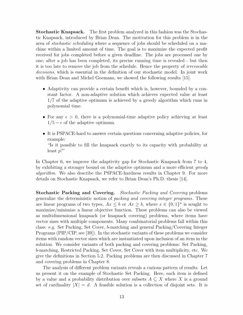
Stochastic Knapsack. The first problem analyzed in this fashion was the Stochas-tic Knapsack, introduced by Brian Dean. The motivation for this problem is in thearea of stochastic scheduling where a sequence of jobs should be scheduled on a ma-chine within a limited amount of time. The goal is to maximize the expected profitreceived for jobs completed before a given deadline. The jobs are processed one byone; after a job has been completed, its precise running time is revealed - but thenit is too late to remove the job from the schedule. Hence the property of irrevocabledecisions, which is essential in the definition of our stochastic model. In joint workwith Brian Dean and Michel Goemans, we showed the following results [15].

• Adaptivity can provide a certain benefit which is, however, bounded by a con-stant factor. A non-adaptive solution which achieves expected value at least1/7 of the adaptive optimum is achieved by a greedy algorithm which runs inpolynomial time.

• For any ǫ > 0, there is a polynomial-time adaptive policy achieving at least1/5 − ǫ of the adaptive optimum.

• It is PSPACE-hard to answer certain questions concerning adaptive policies, forexample:“Is it possible to fill the knapsack exactly to its capacity with probability atleast p?”

In Chapter 6, we improve the adaptivity gap for Stochastic Knapsack from 7 to 4,by exhibiting a stronger bound on the adaptive optimum and a more efficient greedyalgorithm. We also describe the PSPACE-hardness results in Chapter 9. For moredetails on Stochastic Knapsack, we refer to Brian Dean’s Ph.D. thesis [14].

Stochastic Packing and Covering. Stochastic Packing and Covering problemsgeneralize the deterministic notion of packing and covering integer programs. Theseare linear programs of two types, Ax ≤ b or Ax ≥ b, where x ∈ 0, 1n is sought tomaximize/minimize a linear objective function. These problems can also be viewedas multidimensional knapsack (or knapsack covering) problems, where items havevector sizes with multiple components. Many combinatorial problems fall within thisclass: e.g. Set Packing, Set Cover, b-matching and general Packing/Covering IntegerPrograms (PIP/CIP, see [39]). In the stochastic variants of these problems we consideritems with random vector sizes which are instantiated upon inclusion of an item in thesolution. We consider variants of both packing and covering problems: Set Packing,b-matching, Restricted Packing, Set Cover, Set Cover with item multiplicity, etc. Wegive the definitions in Section 5.2. Packing problems are then discussed in Chapter 7and covering problems in Chapter 8.

The analysis of different problem variants reveals a curious pattern of results. Letus present it on the example of Stochastic Set Packing. Here, each item is definedby a value and a probability distribution over subsets A ⊆ X where X is a groundset of cardinality |X| = d. A feasible solution is a collection of disjoint sets. It is

13

known that for deterministic Set Packing, the greedy algorithm provides an O(√

d)-approximation, and there is a closely matching inapproximability result which statesthat for any fixed ǫ > 0, a polynomial-time d1/2−ǫ-approximation algorithm wouldimply NP = ZPP [10]. For Stochastic Set Packing, it turns out that:

• The adaptivity gap can be Ω(√

d) (by an example inspired by the birthdayparadox).

• The adaptivity gap is bounded by O(√

d) (by analyzing an LP bound on theadaptive optimum).

• The proof using an LP leads to a polynomial-time algorithm to find a fixedset of items (i.e., a non-adaptive policy) approximating the adaptive optimumwithin a factor of O(

√d).

• This approximation factor is optimal even if we want to approximate the non-adaptive optimum (due to the d1/2−ǫ-inapproximability result).

This phenomenon appears repeatedly: for Set Packing, b-matching, Set Coverand others. For example, the best approximation factor for Set Cover with itemmultiplicity is O(log d), the adaptivity gap for Set Cover can be Ω(log d) and yet wecan approximate the adaptive optimum by an efficient non-adaptive policy within afactor of O(log d). In general, we design approximation algorithms for most stochasticvariants which are near-optimal even in the deterministic cases.

These results hint at a deeper underlying connection between the quantities we areinvestigating: deterministic approximability, adaptivity gap and stochastic approx-imability. Note that there is no reference to computational efficiency in the notionof adaptivity gap, so a direct connection with the approximability factor would bequite surprising. Another related quantity is the integrality gap of the associatedlinear program: in the cases in question, the integrality gap has the same asymptoticbehavior as well. In Section 5.3, we establish a connection between the integralitygap and the randomness gap for the respective stochastic problem: this is the possiblegap between two instances which differ in the probability distributions of item sizes,but not in the expectations of item sizes. The randomness gap is another boundon stochastic approximability (even by means of an adaptive policy) assuming thatexpectation is the only information available on the item sizes.

Hardness of approximation. We improve some of the previous results on theapproximability of PIP. For general Packing Integer Programs, it was known thata polynomial-time d1/2−ǫ-approximation algorithm for any fixed ǫ > 0 would implyNP = ZPP [10]. We improve this negative result to d1−ǫ. It was also known that

a d1/(B+1)−ǫ-approximation for PIP with A ∈ [0, 1]d×n and ~b = (B, B, . . . , B) (“Re-stricted Packing”) would imply NP = ZPP [10]. We improve this inapproximabilityfactor to d1/B−ǫ.

14

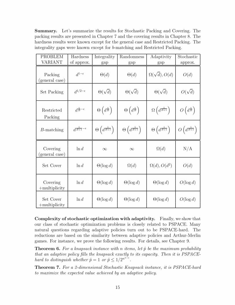
Summary. Let’s summarize the results for Stochastic Packing and Covering. Thepacking results are presented in Chapter 7 and the covering results in Chapter 8. Thehardness results were known except for the general case and Restricted Packing. Theintegrality gaps were known except for b-matching and Restricted Packing.

PROBLEM Hardness Integrality Randomness Adaptivity StochasticVARIANT of approx. gap gap gap approx.

Packing d1−ǫ Θ(d) Θ(d) Ω(√

d), O(d) O(d)(general case)

Set Packing d1/2−ǫ Θ(√

d) Θ(√

d) Θ(√

d) O(√

d)

Restricted d1B−ǫ Θ

(

d1B

)

Θ(

d1B

)

Ω(

d1

B+1

)

O(

d1B

)

Packing

B-matching d1

B+1−ǫ Θ

(

d1

B+1

)

Θ(

d1

B+1

)

Θ(

d1

B+1

)

O(

d1

B+1

)

Covering ln d ∞ ∞ Ω(d) N/A(general case)

Set Cover ln d Θ(log d) Ω(d) Ω(d), O(d2) O(d)

Covering ln d Θ(log d) Θ(log d) Θ(log d) O(log d)+multiplicity

Set Cover ln d Θ(log d) Θ(log d) Θ(log d) O(log d)+multiplicity

Complexity of stochastic optimization with adaptivity. Finally, we show thatour class of stochastic optimization problems is closely related to PSPACE. Manynatural questions regarding adaptive policies turn out to be PSPACE-hard. Thereductions are based on the similarity between adaptive policies and Arthur-Merlingames. For instance, we prove the following results. For details, see Chapter 9.

Theorem 6. For a knapsack instance with n items, let p be the maximum probabilitythat an adaptive policy fills the knapsack exactly to its capacity. Then it is PSPACE-hard to distinguish whether p = 1 or p ≤ 1/2n1−ǫ

.

Theorem 7. For a 2-dimensional Stochastic Knapsack instance, it is PSPACE-hardto maximize the expected value achieved by an adaptive policy.

15

16

Chapter 2

Optimization problems on randomsubgraphs

In a variety of optimization settings, one has to repeatedly solve instances of the sameproblem in which only part of the input is changing. It is beneficial in such cases toperform a precomputation that involves only the static part of the input and possiblyassumptions on the dynamic part. Our goal is to speed up the subsequent solution ofinstances arriving at random. The precomputation could possibly be computationallyintensive.

In telecommunication networks for example, the topology may be considered fixedbut the demands of a given customer (in a network provisioning problem) may varyover time. The goal is to exploit the topology without knowing the demands. Thesame situation happens in performing multicast in telecommunication networks; weneed to solve a minimum spanning tree or Steiner tree problem to connect a group ofusers, but the topology or graph does not change when connecting different groups ofusers. In flight reservation systems, departure and arrival locations and times changefor each request but schedules do not (availability and prices do change as well buton a less frequent basis). Yet another example is for delivery companies; they have tosolve daily vehicle routing problems in which the road network does not change butthe locations of customers to serve do.

Examples of such repetitive optimization problems with both static and dynamicinputs are countless and in many cases it is unclear if one could take any advantage ofthe advance knowledge of the static part of the input. One situation which has beenmuch studied (especially from a practical point-of-view) is for s-t shortest path queriesin large-scale navigation systems or Geographic Information Systems. In that setting,it is too slow to compute from scratch the shortest path whenever a query comes in.Various preprocessing steps have been proposed, often creating a hierarchical view ofthe network, see for example [26].

We study several combinatorial problems for which such precomputation mightbe useful. First, we consider the minimum spanning tree (MST) problem, which isone of the basic optimization problems and it also serves as a building block in moresophisticated algorithms and heuristics. We would like to find a sparse subgraph Q ofa given graph G such that the minimum spanning tree of a random subgraph of G is

17

contained in Q almost always. This would speed up subsequent random MST queries,by restricting our attention to the edges in Q. Our answer would be guaranteed tobe correct with high probability.

In the following chapter, we turn to another problem along these lines where wewould like to approximate the shortest-path metric for random subgraphs, by selectinga priori a subgraph Q whose metric approximates that of a random subgraph. Thiswould then allow us to speed up the solution of any combinatorial problem, basedon the shortest-path metric, such as Steiner Tree, Facility Location or TravelingSalesman. Again, we assume that instances are generated as random subgraphs.

2.1 The MST-covering problem

The MST-covering problem. Assume we are given an edge-weighted graph G =(V, E) with n vertices and m edges and we would like to (repeatedly) find theminimum-weight spanning tree of either a vertex-induced subgraph H = G[W ], W ⊆V (the vertex case) or a subgraph H = (V, F ), F ⊆ E (the edge case). In general,we need to consider the minimum spanning forest, i.e. the minimum spanning treeon each component, since the subgraph might not be connected. We denote this byMST (W ) or MST (F ).

Our primary focus is a random setting where each vertex appears in W indepen-dently with probability p (in the vertex case; we denote W = V (p)); secondly, asetting where each edge appears in F independently with probability p (in the edgecase; we denote F = E(p)). The question we ask is whether there exists a sparse setof edges Q which contains the minimum spanning forest of the random subgraph withhigh probability.

We also address a deterministic setting where we assume that W is obtained fromV by removing a fixed number of vertices, or F is obtained from E by removing afixed number of edges (by a malicious adversary). Then we seek a sparse set of edgesQ containing the minimum spanning forests of all such subgraphs.

More precisely, if the minimum spanning tree is not unique, we ask that Q containssome minimum spanning tree. Alternatively, we can break ties by an arbitrary fixedordering of edges, and require that Q contains the unique minimum spanning tree.This is a stronger requirement and in the following, we will indeed assume that theedge weights are distinct and the minimum spanning trees is unique.

Example. Consider a complete graph G on vertices V = 1, 2, . . . , n where theweight of edge (i, j), i < j is w(i, j) = 2i. Assume that W ⊆ V is sampled uniformly,each vertex with probability 1/2. It is easy to see that MST (W ) is a star of edgescentered at the smallest i in W and connecting i to the remaining vertices in W .The probability that (i, j) ∈ MST (W ) (for i < j) is 1/2i+1 since i, j must bein W and no vertex smaller than i can be in W . Note that when we order theedges (i, j) lexicographically, their probabilities of appearance in MST(W) decreaseexponentially, by a factor of 2 after each block of roughly n edges. If this were alwaysthe case, we could take O(n log n) edges with the largest probability of appearance in

18

1

2

3 4

5

6

78

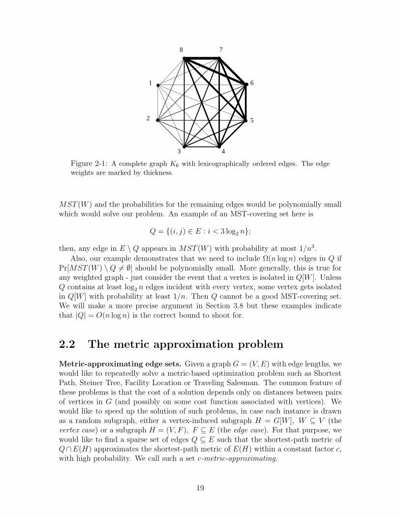
Figure 2-1: A complete graph K6 with lexicographically ordered edges. The edge

weights are marked by thickness.

MST (W ) and the probabilities for the remaining edges would be polynomially smallwhich would solve our problem. An example of an MST-covering set here is

Q = (i, j) ∈ E : i < 3 log2 n;

then, any edge in E \ Q appears in MST (W ) with probability at most 1/n3.

Also, our example demonstrates that we need to include Ω(n log n) edges in Q ifPr[MST (W ) \ Q 6= ∅] should be polynomially small. More generally, this is true forany weighted graph - just consider the event that a vertex is isolated in Q[W ]. UnlessQ contains at least log2 n edges incident with every vertex, some vertex gets isolatedin Q[W ] with probability at least 1/n. Then Q cannot be a good MST-covering set.We will make a more precise argument in Section 3.8 but these examples indicatethat |Q| = O(n log n) is the correct bound to shoot for.

2.2 The metric approximation problem

Metric-approximating edge sets. Given a graph G = (V, E) with edge lengths, wewould like to repeatedly solve a metric-based optimization problem such as ShortestPath, Steiner Tree, Facility Location or Traveling Salesman. The common feature ofthese problems is that the cost of a solution depends only on distances between pairsof vertices in G (and possibly on some cost function associated with vertices). Wewould like to speed up the solution of such problems, in case each instance is drawnas a random subgraph, either a vertex-induced subgraph H = G[W ], W ⊆ V (thevertex case) or a subgraph H = (V, F ), F ⊆ E (the edge case). For that purpose, wewould like to find a sparse set of edges Q ⊆ E such that the shortest-path metric ofQ∩E(H) approximates the shortest-path metric of E(H) within a constant factor c,with high probability. We call such a set c-metric-approximating.

19

Example. In the example of Section 2.1, the MST covering set Q would also be a1-metric-approximating set, i.e. preserving the metric exactly with high probability.This is because the minimum spanning tree of any induced subgraph G[W ] is a starwhich defines the shortest-path metric exactly. However, this phenomenon will turnout to be quite rare and not attainable in general.

2.3 Literature review

2.3.1 MST covering

The absence of complete knowledge of the input data is the defining characteristicof stochastic optimization. Very often, part of the input is random and one has tomake a decision in the first stage without knowing the realization of the stochasticcomponents; these are then revealed and one has to make further decisions. Althoughthe minimum spanning tree problem (as a prototypical combinatorial optimizationproblem) has been considered in a wide variety of settings with incomplete or changingdata, it has not been under the particular viewpoint considered here.

In dynamic graph algorithms, one assumes that the graph is dynamically changingand one needs to update the solution of the problem after each input update. For aminimum spanning tree problem in which edges can be inserted or deleted, the bestknown dynamic algorithm has amortized cost O(log4 n) per operation [24]. This isnot efficient here though, since our instances are changing too drastically.

In the NP-hard Probabilistic MST problem [4], each vertex becomes a “terminal”independently with a given probability. However, the goal here is to find a spanningtree such that the Steiner tree obtained by removing the edges not needed to connectthe terminals has minimum expected cost. Our different model has the advantageof giving a minimum spanning tree (instead of a suboptimal spanning tree) at theexpense of a logarithmic increase in the number of edges.

In practice, graph optimization problems are often solved on a sparse subgraph,and edges which are not included are then priced to see if they could potentiallyimprove the solution found, see for example [1] for the matching problem. Our resultscan therefore be viewed as a theoretical basis for this practice in the case of the MST,and give precise bounds on the sparsity required.

2.3.2 Metric approximation

Sparse subgraphs approximating the shortest-path metric have been considered inample scope, under various restrictions - for geometric graphs, general graphs, withconstrained degrees, restricted structure, etc. Metric-approximating subgraphs areknown as spanners. We say that S ⊂ G is a c-spanner if for any path in G of lengthl there is a corresponding path in S of length at most cl. See for example [13] for asurvey of results about general spanners.

The existence of spanners with a low number of edges is related to the existenceof graphs without short cycles. We say the graph G has girth g, if the length of the

20

shortest cycle is g. A c-spanner for a graph of girth g ≥ c+2 (with unit edge lengths)must be the graph itself, since no edge can be replaced by another path of length atmost c. Therefore the number of edges required in general for a c-spanner is at leastthe extremal number of edges for a graph of girth g = c + 2. It is known that thereare graphs of girth g with n1+1/(g−1) edges (in classical work by Paul Erdos [35]; theproof uses the probabilistic method).

On the other hand, a spanner can be constructed by a construction avoiding cyclesshorter than c + 1, which yields c-spanner of girth at least c + 2 (see [13]). Thus theextremal number of edges for graphs of given girth provides an upper bound on thesize of spanners as well. The best known upper bound on the number of edges for agraph of girth g is O(n1+2/(g−2)) for g ≥ 4 even [3]. So there always exists a c-spannerwith O(n1+2/c) edges.

However, our requirements are stronger than those for a spanner: we ask thatour subgraph Q approximates the metric of G[W ] even when Q is restricted to thesubgraph induced by W . In other words, we are not allowed to use paths in Q leavingthe subset W .

21

22

Chapter 3

Covering the minimum spanningtree of random subgraphs

3.1 The first attempt

Let’s start with the variant of the MST covering problem where vertices are removedat random. For now, assume that each vertex is removed independently with proba-bility 1/2 and denote the set of surviving vertices by W . In this section, we are notgoing to achieve the optimal upper bound, but we develop a simple algorithm whichdemonstrates that at least some non-trivial upper bound exists. Naturally, takingall O(n2) edges of the graph for Q is a valid solution, but we would like to improvesignificantly on this.

The intuitive idea behind this algorithm is that of “path covering”. This is similarto the usual procedure to construct a spanner. Note that in building a minimumspanning tree (consider for example Prim’s algorithm), an edge (u, v) is not used ifthere is a u − v path containing only edges of smaller weight. In such a case, we saythat a path covers (u, v). This does not mean that (u, v) cannot appear in the MSTof a subgraph of G, but it is an indication that (u, v) might not be necessary for ourcovering set Q. Let’s describe our first algorithm now.

Algorithm 1. (given parameters c, r ∈ Z+)

1. Let E1 := E(G). Repeat the following for k = 1, 2, . . . , r.

2. Let Qk := ∅.

3. Process the edges of Ek in the order of increasing edge weights.

4. For each edge (u, v) ∈ Ek, unless it is covered by a path of length at most c inQk, include (u, v) in Qk.

5. If k < r, set Ek+1 := Ek \ Qk and go back to 2.

6. Finally, let Q := ∪rk=1Qk.

23

Q

e

e2

1

Figure 3-1: An example of path covering. The bold edges are already included in

Q. The dashed edges are considered for inclusion; edge e1 is covered by a path of

length 3, while the edge e2 is covered only by a path of length 4.

Note that in each stage k, this algorithm maintains two useful properties. Anyedge which is not in Qk is covered by a path of length at most c; this path uses edgesof smaller weight, which serves to decrease the probability that (u, v) ∈ MST (W ).Secondly, the algorithm avoids all cycles shorter than c + 2 to be created in Qk; thisserves to bound the size of Q.

Lemma 1. For c = 3 and r = ⌊12 lnn⌋, Algorithm 1 finds in polynomial time aset Q of size |Q| ≤ O(n3/2 ln n) such that for W ⊆ V sampled uniformly at random,Pr[MST (W ) ⊆ Q] > 1 − 1/n.

Proof. For each k = 1, 2, . . . , r, Qk is a set of edges avoiding a C4. By a well-knownresult in extremal graph theory [3], |Qk| = O(n3/2). Therefore |Q| = O(rn3/2) =O(n3/2 log n).

Now consider an edge (u, v) ∈ E that we have not chosen in any stage, i.e.(u, v) /∈ ∪r

k=1Qk. For each k, there is a covering u − v path of length 2 or 3. Byconstruction, these paths are edge-disjoint. For a path of length 2, there is probability1/2 that it survives in G[W ]. For a path of length 3, the probability is 1/4.

Note that if two of these paths share a vertex w, then they must be both of length3 and w is a common neighbor of u and v. In that case, we remove the two paths andreplace them by a path of length 2, u−w−v. For two vertex-disjoint paths of length 3,the probability that neither of them survives in G[W ] is (1−1/4)2 which is more thanthe probability of destruction for a single path of length 2. Therefore we may assumethat we have r vertex-disjoint u − v-covering paths of length 3; (u, v) ∈ MST (W )can occur only if u, v ∈ W while none of these paths survive in W :

Pr[(u, v) ∈ MST (W )] ≤ 1

4

(

1 − 1

4

)r

<1

4e−r/4 ≤ 1

n3,

Pr[∃(u, v) ∈ E \ Q; (u, v) ∈ MST (W )] <1

n.

One might try to strengthen the argument by checking for paths longer than 3

24

but in the case of vertex-sampling, c > 3 creates difficulties because of the positivecorrelation among overlapping paths. Still, this idea works in the edge-sampling case.Then we choose c optimally to cover edges by paths of length at most

√ln n which

yields a near-linear bound on Q.

Lemma 2. For c = ⌊√

ln n⌋ and r = ⌊2c+2 ln n⌋, Algorithm 1 finds in polynomial

time a set Q of size O(

n e3√

ln n)

such that for F ⊆ E sampled uniformly at random,

Pr[MST (F ) ⊆ Q] > 1 − 1/n2.

Proof. To estimate the size of Q, note that each Qk is a set of edges avoiding cyclesof length smaller than c + 2, which has size O(n1+2/c) (see [3]). Thus

|Q| = O(rn1+2/c) = O(2cn1+2/c log n) = O(n e3√

ln n).

To prove that Q is a good covering set, note that any (u, v) ∈ E \ Q is coveredby r edge-disjoint paths of length at most c. Each of them has probability at least1/2c of survival and (u, v) ∈ MST (F ) is possible only if none of the r paths survive.Here, the events are independent because of edge-disjointness.

Pr[(u, v) ∈ MST (F )] ≤ 1

2

(

1 − 1

2c

)r

<1

2e−r/2c ≤ 1

n4.

By the union bound over all edges, MST (F ) ⊆ Q with probability at least 1 −1/n2.

Thus we have bounds O(n3/2 log n) for the vertex case and O(n e3√

lnn) for theedge case, respectively. These are actually the best bounds we are able to achieveby efficient deterministic algorithms. Also, note that the covering paths here areguaranteed to have short length. In fact, Q is also a 3-metric-approximating set.We explore this idea further in Chapter 4. In the following, we turn to probabilisticmethods which lead to the asymptotically optimal bound of O(n logn) for the MSTcovering problem.

3.2 The boosting lemma

We start by analyzing the event that a fixed edge appears in the minimum spanningtree of a random induced subgraph. We would like to show that the probability ofthis event cannot be too high for too many edges.

The property of belonging to the minimum spanning tree of an induced subgraphhas a very simple property, and that is down-monotonicity: intuitively, removing morevertices makes an edge only more likely to appear in the MST.

Lemma 3. For an edge (u, v) ∈ E, let X = V \ u, v and let F denote the family ofvertex sets A ⊆ X for which (u, v) is in the minimum spanning forest of the inducedsubgraph G[A ∪ u, v]. Then F is a down-monotone family:

A ∈ F , B ⊆ A =⇒ B ∈ F .

25

Proof. It is easy to see (for example, from Prim’s algorithm) that (u, v) ∈ MST (A∪u, v) if and only if there is no u−v path in G[A∪u, v] using only edges of smallerweight than (u, v). If there is no such path in G[A∪u, v] then there is no such pathin G[B ∪ u, v] either.

For a random A ⊆ X, we say that “A ∈ F” is a down-monotone event. Knowingthat the appearance of an edge in the MST of a random subgraph is a down-monotoneevent will be useful in the following sense: if an edge appears in MST (W ) withprobability ǫ, the probability that it appears in MST (S), where S ⊆ V is a randomset substantially smaller than W , will be much higher than ǫ. This will allow usto bound the number of such edges, because not too many edges can appear in aminimum spanning tree with a large probability.

We prove a general inequality for down-monotone events. We call this inequalitythe boosting lemma, since it states how the probability of a down-monotone event isboosted, when we decrease the sampling probability.

Lemma 4 (The Boosting Lemma). Let X be a finite set and F ⊆ 2X a down-monotone family of subsets of X. Let ~p ∈ [0, 1]n and sample a random subset X(~p)by choosing element i independently with probability pi. Define

σp = Pr[X(~p) ∈ F ].

Let γ ∈ (0, 1) and similarly define σq = Pr[X(~q) ∈ F ] where element i is sampledwith probability qi = 1 − (1 − pi)

γ. Then

σq ≥ σγp .

Proof. We proceed by induction on |X|. For X = ∅ the statement is trivial (σp =σq = 0 or 1). Let a ∈ X, Y = X \ a and define

• F0 = A ⊆ Y : A ∈ F

• F1 = A ⊆ Y : A ∪ a ∈ FBy down-monotonicity, we have F1 ⊆ F0. Next, we express σq by the law of condi-tional probabilities:

σq = Pr[X(~q) ∈ F ] = qa Pr[Y (~q) ∈ F1] + (1 − qa) Pr[Y (~q) ∈ F0]

where Y (~q) denotes a subset of Y sampled with the respective probabilities qi; Y (~q) =X(~q) \ a. We denote ωp = Pr[Y (~p) ∈ F1] and τp = Pr[Y (~p) ∈ F0]. By induction,we can apply the boosting lemma to the down-monotone events F0,F1 ⊆ 2Y : ωq ≥ωγ

p , τq ≥ τγp . We get

σq = qaωq + (1 − qa)τq ≥ (1 − (1 − pa)γ)ωγ

p + (1 − pa)γτγ

p .

Note that ωp ≤ τp because F1 ⊆ F0. It remains to prove the following:

(1 − (1 − p)γ)ωγ + (1 − p)γτγ ≥ (pω + (1 − p)τ)γ (3.1)

26

for any p ∈ [0, 1], γ ∈ (0, 1), 0 ≤ ω ≤ τ . Then we would conclude that

σq ≥ (paωp + (1 − pa)τp)γ = σγ

p

using the law of conditional probabilities for σp = Pr[X(~p) ∈ F ].

We verify Equation 3.1 by analyzing the difference of the two sides: φ(τ) =(1 − (1 − p)γ)ωγ + (1 − p)γτγ − (pω + (1 − p)τ)γ . We show that φ(t) ≥ 0 for t ≥ ω.For t = ω, we have φ(t) = 0. By differentiation,

φ′(t) = γ(1 − p)γtγ−1 − γ(1 − p)(pω + (1 − p)t)γ−1

= γ(1 − p)γtγ−1

(

1 −(

(1 − p)t

pω + (1 − p)t

)1−γ)

≥ 0.

Therefore φ(t) ≥ 0 for any t ≥ ω which completes the proof.

Note. The boosting lemma is tight for F = 2A, A ⊂ X in which case σp =(1−p)|X\A|. This form of the lemma is the most general we have found; more restrictedversions are easier to prove. For probabilities pi, qi satisfying (1−pi) = (1−qi)

k, k ∈ Z,there is a simple probabilistic proof using repeated sampling:

Sample independently subsets Yj = X(~q), j = 1, 2, . . . , k, and set Y = Y1 ∪ Y2 ∪. . . ∪ Yk. Element i has probability (1 − qi)

k = (1 − pi) that it does not appear inany Yj , therefore Y is effectively sampled with probabilities pi. Then we get, fromthe monotonicity of F :

σp = Pr[Y ∈ F ] ≤ Pr[∀j; Yj ∈ F ] = σkq .

Another special case is when the sampling probability p is the same for all elementsand σp = (1−p)k for some k ∈ Z. Then we can argue by the Kruskal-Katona theoremthat F contains at least

(

n−ka

)

subsets of size a for any a ≤ n− k, which implies thatσq ≥ (1 − q)k for any q ≤ p. It is not clear if this applies to σp = (1 − p)k fornon-integer k.

In [6], Bollobas and Thomason prove a lemma about down-monotone events whichapplies to random subsets of fixed size: If Pr is the probability that a random subsetof size r is in F , then for any s ≤ r,

P rs ≥ P s

r .

Considering that the two random models are roughly equivalent (instead of samplingwith probability p, take a random subset of size pn), this lemma has a very similarflavor to ours. However, putting the two random models side by side like this, theBollobas-Thomason lemma is weaker; for example, compare p = 1 − 1/n, q = 1/2and r = n − 1, s = n/2. Our boosting lemma implies σq ≥ (σp)

1/ log n. The Bollobas-Thomason lemma says only Ps ≥

√Pr.

27

3.3 Covering the MSTs of random vertex-induced

subgraphs

Now we prove the bound on the size of covering sets for the case of randomly sampledvertices. As noted before, for any edge (u, v) ∈ E, the event that (u, v) ∈ MST (W ),conditioned on u, v ∈ W , is down-monotone. Let’s denote

σp(u, v) = PrW [(u, v) ∈ MST (W ) | u, v ∈ W ]

where W = V (p) contains each vertex independently with probability p.

Lemma 5. For a weighted graph G on n vertices, 0 < p < 1, and k ≥ 1/p, let

Q(p)k = (u, v) ∈ E : σp(u, v) ≥ (1 − p)k−1.

Then|Q(p)

k | < ekn.

Proof. Sample a random subset S = V (q), with probability q = 1/k ≤ p. For every

edge (u, v) ∈ Q(p)k , we have σp(u, v) ≥ (1−p)k−1, and therefore by the boosting lemma

with γ = ln(1−q)ln(1−p)

, we get σq(u, v) ≥ (1 − q)k−1. Consequently, Q(p)k ⊆ Q

(q)k and

Pr[(u, v) ∈ MST (S)] = q2σq(u, v) ≥ 1

k2(1 − q)k−1 >

1

ek2,

E[|MST (S)|] ≥∑

(u,v)∈Q(p)k

Pr[(u, v) ∈ MST (S)] >|Q(p)

k |ek2

.

On the other hand, the size of the minimum spanning forest on S is at most the sizeof S, and so

E[|MST (S)|] ≤ E[|S|] =n

k.

Combining these two inequalities, we get |Q(p)k | < ekn.

Theorem 8. Let G be a weighted graph on n vertices, 0 < p < 1, and c > 0. Letb = 1/(1 − p). Then there exists a set Q ⊆ E of size

|Q| ≤ e(c + 1)n logb n + O(n)

such that for a random W = V (p),

PrW [MST (W ) ⊆ Q] > 1 − 1

nc.

Proof. Order the edges by the decreasing values of σp(u, v). Partition the sequenceinto blocks B1, B2, . . . ⊂ E of size ⌈en⌉. Lemma 5 implies that for any (u, v) ∈ Bk+1,k ≥ 1/p,

Pr[(u, v) ∈ MST (W )] = p2 σp(u, v) < p2(1 − p)k−1.

28

Define Q as the union of the first h = ⌈(c + 1) logb n⌉ + 2 blocks, Q =⋃h

k=1 Bk.We have h ≥ 1/p (for p ≥ 1/2 it’s obvious that h ≥ 2 ≥ 1/p, and for p < 1/2,h > logb n > ln n

2p> 1/p for n > e2). So we can apply the above bound to blocks

starting from h + 1:

Pr[MST (W ) \ Q 6= ∅] ≤∑

(u,v)∈E\QPr[(u, v) ∈ MST (W )]

≤∞∑

k=h+1

⌈en⌉p2(1 − p)k−2 = ⌈en⌉p(1 − p)h−1 <⌈en⌉p(1 − p)

nc+1<

1

nc.

3.4 Improving the constant factor

In the results of Lemma 5 and Theorem 8, we get a factor of e which however seemsto be an artifact of the probabilistic proof. In fact it is possible that the best upperbound has a constant factor of 1. The example in Section 3.8 shows that this wouldbe tight. In this section, we show that e is indeed just a product of the proof and weprove a somewhat improved constant factor.

Lemma 6. For the set Q(p)k from Lemma 5 and any k ≥ 1/p,

|Q(p)k | < (1 + e/2)kn.

Proof. Consider more carefully the argument bounding |Q(p)k |:

pn ≥ E[|MST (V (p))|] ≥∞∑

l=1

|Q(p)l \ Q

(p)l−1| p2(1 − p)l−1 =

∞∑

l=1

|Q(p)l | p3(1 − p)l−1,

i.e.

n ≥∞∑

l=1

|Q(p)l | p2(1 − p)l−1.

Our previous argument basically replaces all the terms for l < k by zero, which leadsto the factor of e (for p = 1/k). However, we can get a better upper bound, if wecan lower bound these terms as well. And that is certainly possible - let’s assumethat G is a complete graph (without loss of generality for the upper bound). Then

Q(p)l must be l-vertex-connected, otherwise there is an edge (u, v) ∈ E \Q

(p)l which is

not covered by l vertex-disjoint paths in Q(p)l which would imply σp(u, v) ≥ (1 − p)l.

Therefore |Q(p)l | ≥ ln/2.

More generally, assume that

• ∀l < k; |Q(p)l | ≥ γln, for some constant γ > 0.

29

Then we get, replacing |Q(p)l | by γln for l < k and by |Q(p)

k | for l > k,

n ≥k−1∑

l=1

γlnp2(1 − p)l−1 +

∞∑

l=k

|Q(p)k |p2(1 − p)l−1

= γnk−1∑

l=1

k−1∑

j=l

p2(1 − p)j−1 + |Q(p)k | p(1 − p)k−1

= γn

k−1∑

l=1

p((1 − p)l−1 − (1 − p)k−1) + |Q(p)k | p(1 − p)k−1

= γn(1 − (1 − p)k−1(1 + p(k − 1))) + |Q(p)k | p(1 − p)k−1.

This implies a bound on |Q(p)k |, namely

|Q(p)k | ≤

(

1 − γ

(1 − p)k−1+ γ(1 + p(k − 1))

)

n

p. (3.2)

Using the l-connectivity argument, we can use γ = 1/2, and for q = 1/k we get

|Q(q)k | ≤

(

1/2

(1 − q)k−1+ 1

)

n

q≤(e

2+ 1)

kn.

For p ≥ q, we apply the boosting lemma which as in the proof of Lemma 5 impliesthat Q

(p)k ⊆ Q

(q)k . Therefore the bound holds for any p ≥ 1/k as well.

As a direct consequence, we get an improved version of Theorem 8.

Theorem 9. Let G be a weighted graph on n vertices, 0 < p < 1, and c > 0. Letb = 1/(1 − p). Then there exists a set Q ⊆ E of size

|Q| ≤ (1 + e/2)(c + 1)n logb n + O(n)

such that for a random W = V (p),

PrW [MST (W ) ⊆ Q] > 1 − 1

nc.

3.5 Covering the MSTs of subgraphs of fixed size

Directly from Lemma 6, we also get the following interesting implication for the“deterministic version” of the problem, where at most k − 1 vertices can be removedarbitrarily.

Corollary 1. For any weighted graph G on n vertices, and k ∈ Z+, there exists a setQk ⊆ E of size

|Qk| < (1 + e/2)kn

which contains MST (W ) for any |W | > n − k.

30

Proof. Let Qk =⋃

|W |>n−k MST (W ). For k = 1 the lemma is trivial (Q1 is the

minimum spanning tree of G). For k ≥ 2, choose p = 1/2 and consider Q(p)k as

defined in Lemma 5. Lemma 6 which states that |Q(p)k | < (1 + e/2)kn. For any

edge (u, v) which appears in MST (W ) for |W | > n − k, σp(u, v) ≥ (1 − p)k−1, sincethe vertices in V \ W are removed with probability at least (1 − p)k−1; therefore

Qk ⊆ Q(p)k .

Observe that the set Qk can be found in polynomial time. For every edge (u, v),its membership in Qk can be tested by computing the vertex connectivity betweenvertices u, v in the subgraph of edges lighter than (u, v). By Menger’s theorem,(u, v) ∈ Qk if and only if there are no k vertex-disjoint u − v paths using edges ofsmaller weight than (u, v). This, however, does not seem to imply a bound on the sizeof Qk easily. The only way we can prove our bound is through probabilistic reasoning.

It is not difficult to see that |Q1| ≤ n− 1 and |Q2| ≤ 2n− 3. It is also possible todefine edge weights so that Qk must contain (n−1)+(n−2)+· · ·+(n−k) = kn−

(

k+12

)

edges (see Section 3.8 for an example). We conjecture this to be the actual tight upper

bound. Similarly, we conjecture that kn −(

k+12

)

is the best possible bound on |Q(p)k |

in Lemma 5 (and this would be also achieved for the graph described in Section 3.8).The same question in the edge case is easier to answer. The number of edges in

all MSTs obtained upon removing at most k − 1 edges can be bounded by k(n − 1),by finding the minimum spanning tree and removing it from the graph, repeatedlyk times. (Which also works for multigraphs, and more generally for matroids.) Forsimple graphs, we can prove a bound of kn −

(

k+12

)

which is tight (see the examplesconstructed in Section 3.8).

Lemma 7. For any (simple) weighted graph on n vertices and 1 ≤ k ≤ n, there existsa set Qk ⊆ E of size

|Qk| ≤k∑

i=1

(n − i) = kn −(

k + 1

2

)

which contains the minimum spanning forest MST (F ) for any |F | > m − k.

Proof. Let Qk =⋃

|F |>m−k MST (F ). We proceed by induction on n. For n = k, it is

trivial that |Qk| ≤(

n2

)

. So assume n > k.Consider the heaviest edge e∗ ∈ Qk. Since e∗ ∈ MST (F ) for some |F | > m − k,

there is a cut δ(V1) = (u, v) ∈ E : u ∈ V1, v /∈ V1 such that e∗ is the lightest edge inδ(V1) ∩ F . Consequently Qk ∩ δ(V1) ⊆ (E \ F ) ∪ e∗, which means that at most kedges of Qk are in the cut δ(V1). Let V2 = V \ V1 and apply the inductive hypothesison G1 = G[V1] and G2 = G[V2], and their respective MST-covering sets Qk,1, Qk,2. Weuse the following characterization of Qk: (u, v) ∈ Qk ⇔ there are no k edge-disjointu− v paths in the subgraph of edges lighter than (u, v) (again by Menger’s theorem,for edge connectivity). Since the edge connectivity in G is at least as strong as theedge connectivity in G1 or G2, it follows that Qk[V1] ⊆ Qk,1, Qk[V2] ⊆ Qk,2 and weget

|Qk| ≤ |Qk,1| + |Qk,2| + k.

31

Let n1 = |V1|, n2 = |V2|; n = n1 + n2 > k. We distinguish two cases:

• If one of n1, n2 is at least k, assume it is n1. By the inductive hypothesis,|Qk,1| ≤

∑ki=1 (n1 − i), and |Qk,2| ≤ k(n2 − 1) (which holds for any n2, smaller

or larger than k), so

|Qk| ≤k∑

i=1

(n1 − i) + k(n2 − 1) + k =

k∑

i=1

(n − i).

• If both n1, n2 < k, then we estimate simply |Qk,1| ≤(

n1

2

)

, |Qk,2| ≤(

n2

2

)

. We get

|Qk| ≤(

n1

2

)

+

(

n2

2

)

+ k ≤ k(n1 − 1)

2+

k(n2 − 1)

2+ k =

kn

2≤

k∑

i=1

(n − i).

3.6 Algorithmic construction of covering sets

It is natural to ask whether the covering sets can be found efficiently. In the de-terministic case, we have shown that this is quite straightforward (Section 3.5). Forthe probabilistic case, we have shown deterministic algorithms in Section 3.1, but thecovering sets obtained there are larger than optimal. Here, we would like to find cov-ering sets of size that is implied by the boosting lemma. However, we have to keep inmind that it is not possible to test whether (u, v) ∈ Q

(p)k directly. This would amount

to calculating the u-v-reliability in the graph of edges lighter than (u, v), which is a#P-complete problem [33].

Still, we can find a covering set Q with an efficient randomized algorithm, whichtakes advantage of the boosting lemma as well. It is a Monte Carlo algorithm, in thesense that it finds a correct solution with high probability, but the correctness of thesolution cannot be verified easily.

Algorithm 2. Given G = (V, E), w : E → R, 0 < p < 1, c > 0.

• Let b = 1/(1 − p) and k = ⌈(c + 2) logb n⌉ + 1.

• Repeat the following for i = 1, . . . , r = ⌈32ek2 ln n⌉:

– Sample Si ⊆ V , each vertex independently with probability q = 1/k.

– Find Ti = MST (Si).

• For each edge, include it in Q if it appears in at least 16 lnn different Ti’s.

The running time of Algorithm 2 is determined by the number of calls to an MSTprocedure, which is O(logb n ln n). Since a minimum spanning forest can be foundin time O(mα(m, n)) deterministically [9] or O(m) randomized [28], for constantb = 1/(1 − p) we get a running time near-linear in m.

32

Theorem 10. Algorithm 2 finds with high probability a set Q ⊆ E such that

|Q| ≤ 2e(c + 2)n logb n + O(n)

and for a random W = V (p),

PrW [MST (W ) ⊆ Q] > 1 − 1

nc.

Proof. Let k = ⌈(c+2) logb n⌉+1, r = ⌈32ek2 ln n⌉ and Q(p)k = (u, v) ∈ E : σp(u, v) ≥

(1− p)k−1. We will argue that (1) Q(p)k ⊆ Q with high probability, (2) Q

(p)k is a good

covering set, and (3) |Q| ≤ 2ekn + O(n).

Let Si = V (q), q = 1/k, and Ti = MST (Si). As in the proof of Theorem 8,k ≥ 1/p (for n large enough), therefore q ≤ p and by the boosting lemma, for any

(u, v) ∈ Q(p)k ,

Pr[(u, v) ∈ Ti] ≥ q2(1 − q)k−1 ≥ 1

ek2.

Denoting by t(u, v) the number of Ti’s containing edge (u, v), we get E[t(u, v)] ≥r/(ek2) ≥ 32 lnn. By Chernoff bound (see [34, Theorem 4.2]; Pr[X < (1 − δ)µ] <e−µδ2/2), with µ ≥ 32 lnn, δ = 1/2: Pr[t(u, v) < 16 ln n] < e−4 ln n = 1/n4, and thus

Pr[∃(u, v) ∈ Q(p)k ; t(u, v) < 16 lnn] < 1/n2. Therefore with high probability, all edges

in Q(p)k are included in Q. On the other hand, Q

(p)k contains MST (W ) with high

probability (with respect to a random W = V (p)):

Pr[MST (W ) \ Q(p)k 6= ∅] ≤

∑

(u,v)∈E\Q(p)k

Pr[(u, v) ∈ MST (W )] < n2p2(1 − p)k−1 <1

nc.

Now we estimate the size of Q. For k ≥ n/(4e), the condition |Q| ≤ 2ekn + O(n)is satisifed trivially. So assume k < n/(4e). Since we are sampling Si = V (q), wehave E[|Si|] = qn, and E [

∑ri=1 |Ti|] ≤ E [

∑ri=1 |Si|] ≤ rqn. We can use the Chernoff

bound again ([34, Theorem 4.1]; Pr[X > (1 + δ)µ] < e−µδ2/3), with µ ≤ rqn andδ = 10 lnn/(rq):

Pr

[

r∑

i=1

|Si| > (rq + 10 lnn)n

]

< e−100n ln2 n/(3rq) < e−n ln n/ek <1

n4.

In Q, we include only edges which appear in at least 16 lnn different Ti’s, and |Ti| ≤|Si|, so the number of such edges is, with high probability,

|Q| ≤∑ |Si|16 lnn

≤ (rq + 10 lnn)n

16 lnn= 2ekn + O(n).

33

3.7 Covering minimum-weight bases in matroids

Next, we consider the variant of the problem where the subgraph is generated bytaking a random subset of edges E(p). We approach this problem more generally,in the context of matroids. The matroid in this case would be the graphic matroiddefined by all forests on the ground set E. In general, consider a weighted matroid(E,M, w), where w : E → R. Let m denote the size of the ground set E and n therank of M, i.e. the size of a largest independent set. If the weights are distinct, thenany subset F ⊆ E has a unique minimum-weight basis MB(F ), which in the caseof graphs corresponds to the minimum-weight spanning forest. These bases satisfyexactly the monotonicity property that we used previously.

Lemma 8. For an element e ∈ E, let X = E \ e and let F denote the family ofsubsets A ⊆ X for which e is in the minimum-weight basis of the matroid induced byA ∪ e. Then F is a down-monotone family:

A ∈ F , B ⊆ A =⇒ B ∈ F .

Proof. If e ∈ MB(A ∪ e), it means that there is no circuit in A∪ e in which e isthe largest-weight element. However, then there is no such circuit in B ∪ e either,and therefore e ∈ MB(B ∪ e).

Thus, we can apply the same machinery to matroids. Define

σp(e) = PrF [e ∈ MB(F ) | e ∈ F ]

where F = E(p) is a random subset of elements, sampled with probability p. We getstatements analogous to the vertex case. It is interesting to notice that the boundsgiven in these lemmas depend only on the rank of the matroid, irrespective of thesize of the ground set.

Lemma 9. For a weighted matroid (E,M, w), of rank n, 0 < p < 1 and k ≥ 1/p, let

Q(p)k = e ∈ E : σp(e) ≥ (1 − p)k−1.

Then|Q(p)

k | < ekn.

Proof. Sample a random subset S = E(q), each element with probability q = 1/k ≤ p.

For any e ∈ Q(p)k , σp(e) ≥ (1 − p)k, therefore the boosting lemma implies that

Pr[e ∈ MB(S)] ≥ q σq(e) ≥1

k

(

1 − 1

k

)k−1

>1

ek.

Summing over all e ∈ Q(p)k , we get

E[|MB(S)|] ≥∑

e∈Q(p)k

Pr[e ∈ MB(S)] >|Q(p)

k |ek

.

34

On the other hand, any independent set in M has size at most n, therefore E[|MB(S)|] ≤n which implies |Q(p)

k | < ekn.

Theorem 11. For any weighted matroid (E,M, w) of rank n, 0 < p < 1, c > 0, andb = 1/(1 − p), there exists a set Q ⊆ E of size

|Q| ≤ e(c + 1)n logb n + O(n/p)

such that for a random F = E(p),

PrF [MB(F ) ⊆ Q] > 1 − 1

nc.

Proof. Order the elements of E by decreasing values of σp(e). Partition the sequenceinto blocks B1, B2, . . . ⊂ E of size ⌈en⌉. Lemma 9 implies that for any e ∈ Bk+1,k ≥ 1/p:

Pr[e ∈ MB(F )] = p σp(e) < p(1 − p)k−1.

Take the first h = ⌈(c+1) logb n+2/p⌉+1 blocks: Q =⋃h

k=1 Bk. Then, since h ≥ 1/p:

Pr[MB(F ) \ Q 6= ∅] ≤∑

e∈E\QPr[e ∈ MB(F )] ≤

∞∑

k=h+1

⌈en⌉p(1 − p)k−2

= ⌈en⌉(1 − p)h−1 ≤ ⌈en⌉(1 − p)2/p

nc+1<

1

nc.

The forests in a graph on n + 1 vertices form a matroid of rank n, and minimum-weight bases correspond to minimum spanning forests. Therefore this solves the edgeversion of the problem as well:

Corollary 2. For any weighted graph G on n + 1 vertices, 0 < p < 1, c > 0 andb = 1/(1 − p), there exists a set Q ⊆ E(G) of size

|Q| ≤ e(c + 1)n logb n + O(n/p)

such that for a random F = E(p),

PrF [MST (F ) ⊆ Q] > 1 − 1

nc.

Also, we get a randomized algorithm finding the covering set for any weightedmatroid (E,M, w); the algorithm makes O(logb n lnm) calls to a minimum-weightbasis procedure.

Algorithm 3.

• Let b = 1/(1 − p) and k = ⌈(c + 2) logb n⌉ + 1.

35

• Repeat the following for i = 1, . . . , r = ⌈16ek ln m⌉:

– Sample Si ⊆ E, each element independently with probability q = 1/k.

– Find Ti = MB(Si).

• For each edge, include it in Q if it appears in at least 8 lnm different Ti’s.

Theorem 12. Algorithm 3 finds with high probability a set Q ⊆ E such that

|Q| ≤ 2e(c + 2)n logb n + O(n)

and for a random F = E(p),

PrF [MB(F ) ⊆ Q] > 1 − 1

nc.

Proof. Let k = ⌈(c + 2) logb n⌉ + 1, r = ⌈16ek ln m⌉ and Q(p)k = e ∈ E : σp(e) ≥

(1 − p)k−1. We claim that (1) Q(p)k ⊆ Q with high probability, (2) Q

(p)k is a good

covering set and (3) Q is not too large. As in the proof of Theorem 8, q = 1/k ≤ p for

n large enough, therefore for any e ∈ Q(p)k , Si = E(q) and Ti = MB(Si), the boosting

lemma implies

Pr[e ∈ Ti] = q σq(e) >1

ek.

Letting te denote the number of Ti’s containing element e, we obtain E[te] ≥ r/(ek) ≥16 lnm. By the Chernoff bound, Pr[te < 8 lnm] < e−2 ln m = 1/m2, implying that

Pr[∃e ∈ Q(p)k ; te < 8 lnm] < 1/m. Therefore with high probability, all edges in Q

(p)k

are included in Q.On the other hand, Q

(p)k contains MB(F ) with high probability: Consider the

elements in E \ Q. We order them in a sequence of decreasing values of σp(e), andagain divide them into blocks B1, B2, . . . as before. Since we have included all edgeswith σp(e) ≥ (1 − p)k−1, in the first k blocks the values of σp(e) cannot be largerthan as (1 − p)k−1. However, then the l-th block can have values of σp(e) at mostσp(e) ≤ (1 − p)l−2 (by Lemma 9). Thus

Pr[MB(F ) \ Q 6= ∅] ≤ p

(

k(1 − p)k−1 +

∞∑

l=k+1

(1 − p)l−2

)

⌈en⌉

≤ (kp + 1)⌈en⌉nc+2

=O(lnn)

nc+1<

1

nc

for large n. Finally, we estimate the size of Q. We have∑r

i=1 |Ti| ≤ rn. Every elemente ∈ Q appears in 8 ln m different Ti’s, therefore

|Q| ≤∑ |Ti|8 lnm

≤ 2ekn + O(n).

36

3.8 Lower bounds

For both variants of the problem, we have a closely matching lower bound on the sizeof Q, even if we want to achieve a constant probability of covering the MST. We get alower bound of Ω(n logb(n/ lnn)) for p > ln n/n in the edge case and Ω(n logb(pn/5))for p > 5/n in the vertex case. Both bounds reduce to Ω(n logb n), for a wide rangeof p, namely the lower bound of Ω(n logb n) holds for p ≥ 1/nγ, γ < 1.

The constructions for the vertex and edge variants are different; first let’s describethe edge variant which is simpler.

Lemma 10. For any n > ee2, ln n

n≤ p < 1, there is a weighted graph G on n vertices,

such that if

Pr[MST (E(p)) ⊆ Q] ≥ 1

e

then |Q| > ln −(

l+12

)

where l = ⌊logb(n/ ln n)⌋.

Proof. Consider the complete graph Kn with edge weights ordered lexicographically.For i < j, let

wij = ni + j

(see Figure 2-1). Let F = E(p) be a random subset of edges. For each edge (j, k),j < k, consider an event Ajk, which occurs when

(j, k) ∈ F & ∀i < j; (i, k) /∈ F.

Due to the ordering of edge weights, Ajk implies that (j, k) ∈ MST (F ), since it is thelightest edge in F , incident with vertex k. Also, for given k, Ajk can occur only forone value of j. For a set Q of given size, we estimate the probability that Ajk occursfor some (j, k) ∈ E \ Q:

Let Jk = j : j < k, (j, k) ∈ E \Q. Since the events Ajk for different elements ofJk are disjoint,

Pr[⋃

j∈Jk

Ajk] =∑

j∈Jk

p(1 − p)j−1.

The events⋃

j∈JkAjk for different k’s are mutually independent, since the set of edges

involved for different Jk’s are disjoint. Therefore:

Pr[MST (F ) ⊆ Q] ≤ Pr[⋂

(j,k)∈E\QAjk] =

∏

k

Pr[⋂

j∈Jk

Ajk]

=∏

k

(1 −∑

j∈Jk

p(1 − p)j−1) ≤ exp

−∑

(j,k)∈E\Qp(1 − p)j−1

.

For a given size of Q, the last expression is maximized when Q contains edges(j, k) with minimum possible values of j. Assume that Q contains all the edges (j, k)

37

431 2 65

Figure 3-2: The lower bound example for random sampling of vertices. Edge

weights are marked by thickness.

for j = 1, 2, . . . l. Then |Q| =∑l

j=1 (n − j) = ln −(

l+12

)

and

∑

(j,k)∈E\Qp(1 − p)j−1 =

n−1∑

j=l+1

(n − j)p(1 − p)j−1.

Let’s denote this sum by S(l). As can be verified by backward induction on l,

S(l) =

(

n − l − 1

p

)

(1 − p)l +1

p(1 − p)n.

We have that for any Q of size at most ln −(

l+12

)

, Pr[MST (F ) ⊆ Q] ≤ e−S(l).Let’s choose l = ⌊logb(n/ ln n)⌋. Then, for p ≥ ln n

n,

S(l) ≥(

n − logb

( n

ln n

)

− 1

p

)

ln n

n≥(

n − ln n − ln ln n + 1

p

)

ln n

n≥ ln ln n − 1.

Therefore, for any set Q of size at most ln−(

l+12

)

, Pr[MST (W ) ⊆ Q] ≤ e−S(l) < 1/e

for n > ee2.

Lemma 11. For any n > 5, and p ≥ 5/n, there exists a weighted graph G on nvertices, such that if

Pr[MST (V (p)) ⊆ Q] ≥ 1

e

then |Q| > ln −(

l+12

)

where l = ⌊logb(np/5)⌋.

Proof. Let G be the complete graph Kn. Consider the vertices placed on a lineuniformly and define edge weights by distances between pairs of vertices, breakingties arbitrarily, for example:

wij = n|j − i| + i.

Let W = V (p) be a random subset of vertices. For each edge (j, k), j < k, consideran event Ajk as a boolean function of W :

Ajk(W ) ⇐⇒ j ∈ W, k ∈ W & ∀i; j < i < k ⇒ i /∈ W.

38

This event is equivalent to (j, k) ∈ MST (W ), since (j, k) must be in G[W ] and nopath connecting j, k via a vertex in between can be in G[W ]. However, we have tobe more careful here, because these events are not necessarily independent, whichmight ruin our bound on the probability of their union. Therefore, we have to imposean additional condition which we deal with later. Assume that C is a set of edgessatisfying

(*) There is no pair of edges (i, j), (j, k) ∈ C such that i < j < k.

Then we claim that the events Ajk for (j, k) ∈ C are never positively correlated.More specifically, if (u0, v0), (u1, v1), . . . (uk, vk) ∈ C, ui < vi, then

Pr[Au1v1 ∩ Au2v2 ∩ . . . Aukvk| Au0v0 ] ≤ Pr[Au1v1 ∩ Au2v2 ∩ . . . Aukvk

]. (3.3)

We prove this in the following way: For any W ⊆ V , define W ′ = W ∪ u0, v0 \ i :u0 < i < v0. Then Au0v0(W

′) is true by definition. In fact, if W = V (p) is a randomsubset, W ′ is a random subset sampled in the same way as W , but conditioned onAu0v0 .

Now consider the other edges, (u1, v1), . . . (uk, vk). Let’s call an edge (ui, vi) “in-terfering” with (u0, v0), if its interval [ui, vi] intersects [u0, v0]. Property (∗) impliesthat the intervals [u0, v0], [ui, vi] cannot share exactly one point, so either one of ui, vi

is an internal point of [u0, v0], or one of u0, v0 is an internal point of [ui, vi]. Eitherway, Auivi

(W ′) cannot be true, because then ui and vi ought to be in W ′ and all ver-tices inside [ui, vi] ought not to be in W ′ which is impossible. Therefore, Auivi

(W ′) isalways false for (ui, vi) interfering with (u0, v0). On the other hand, if an edge (ui, vi)is not interfering with (u0, v0), then Auivi

(W ′) if and only if Auivi(W ), because W ′

does not differ from W on the vertices outside of [u0, v0].

Thus we have demonstrated that in any case, Auivi(W ) ⇒ Auivi

(W ′), and W ′

corresponds to random sampling conditioned on Au0v0 , which implies

Pr[Au1v1 ∩ Au2v2 ∩ . . . Aukvk| Au0v0 ] ≥ Pr[Au1v1 ∩ Au2v2 ∩ . . . Aukvk

].

This is equivalent to Eq. 3.3. As a consequence, we get

Pr[⋂

e∈C

Ae] ≤∏

e∈C

Pr[Ae].

For a set C satisfying (∗), we can now estimate the probability that none of theseedges appear in MST (W ):

Pr[C ∩ MST (W ) = ∅] = Pr[⋂

(j,k)∈C

Ajk] ≤∏

(j,k)∈C

Pr[Ajk]

=∏

(j,k)∈C

(1 − p2(1 − p)|k−j|−1) < exp

−∑

(j,k)∈C

p2(1 − p)|k−j|−1

.

Suppose that Q has size at most∑l

j=1 (n − j) = ln −(

l+12

)

. The optimal way to

39

minimize∑

(j,k)∈E\Q p2(1 − p)|k−j|−1 is to choose Q to contain all the edges of lengthat most l. Then we have

∑

(j,k)∈E\Qp2(1 − p)|k−j|−1 =

n−1∑

j=l+1

(n − j)p2(1 − p)j−1 = p S(l)

where S(l) is defined in the previous proof, S(l) = (n− l− 1p)(1− p)l + 1

p(1− p)n. We

choose l = ⌊logb(np/5)⌋ and then:

p S(l) ≥ (p(n−l)−1)(1−p)l ≥ (p(n−logb(np/5))−1)5

np≥ 5

(

1 − ln(np/5) + 1

np

)

≥ 4.

Thus we have∑

(j,k)∈E\Q p2(1 − p)|k−j|−1 ≥ 4 for any Q of size at most ln−(

l+12

)

. Now

we apply the probabilistic method to choose a suitable subset of E \Q. We sample auniformly random subset of vertices S. Let C = (j, k) ∈ E\Q : j < k, j ∈ S, k /∈ S.For each edge in E \ Q, there is probability 1/4 that it appears in C. Therefore

E[∑

(j,k)∈C

p2(1 − p)|k−j|−1] ≥ 1

4

∑

(j,k)∈E\Qp2(1 − p)|k−j|−1 ≥ 1

and there exists a set C which achieves at least this expectation. Due to the con-struction of C, it satisfies condition (*), and we can conclude that

Pr[MST (W ) ⊆ Q] ≤ Pr[C ∩ MST (W ) = ∅] < e−1.

This is a contradiction, and so Q must be larger than ln −(

l+12

)

.

40

Chapter 4

Metric approximation for randomsubgraphs

4.1 Covering shortest paths

We continue in the spirit of Chapter 3 where the goal was to find a sparse set ofedges covering with high probability the solution of an optimization problem (MST,in particular) for a random subgraph. Consider another fundamental optimizationproblem on graphs: the Shortest Path.

Assume that we have a graph G and two designated vertices s, t ∈ V . Recall thatwe denote by V (p) a random subset of V where each vertex is sampled independentlywith probability p. We would like to find a set of edges Q such that for a randominduced subgraph G[W ], W = V (p)∪s, t, Q contains a shortest s− t path in G[W ]with high probability. It turns out that in contrast to the MST problem, ShortestPath is not amenable to good covering sets.

Example. Consider a graph G = (V, E) where

• V =⋃k

i=1 Ai ∪⋃k

i=1 Bi

• E =⋃k

i=1 E(Ai) ∪⋃k

i=1 E(Bi) ∪ H .

• Ai = s, ai1, ai2, . . . , ail

• E(Ai) is a path s − ai1 − ai2 − . . . − ail

• Bi = t, bi1, bi2, . . . , bil

• E(Bi) is a path t − bi1 − bi2 − . . . − bil

• H is a complete bipartite graph (ail, bjl) : 1 ≤ i, j ≤ k.

• The edges in E(Ai) and E(Bi) have zero length, while the edges in H have unitlength.

41

s t

H

0

0 0 0 0

0

1

Figure 4-1: A counterexample to s− t-shortest path covering, for k = 8 and l = 3.

We set k = 2l, n = |V | = l2l+1 + 2. Sample W ⊆ V , each vertex with probability1/2 except s, t which are always in W . Consider the event that Ai is the unique pathamong A1, A2, . . . , Ak which survives in G[W ]: this happens with probability 2−l(1−2−l)k−1 > 1/ek. Independently, Bj is the unique surviving path among B1, B2, . . . , Bk,with probability 1/ek. Thus with probability 1/(ek)2, there is a unique shortest s− tpath (of length 1), using the surviving paths Ai, Bj and the edge (ail, bjl) ∈ H . Thisholds for every edge in H with the same probability and the corresponding events aredisjoint. If h = |H \ Q|, there is probability at least h/(ek)2 that Q doesn’t containthe shortest path. Therefore Q must contain Ω(k2) edges in H , for instance k2/2,otherwise the probability of missing the shortest path is at least 1/2e2. We conclude:

Lemma 12. There are graphs on n vertices such that if Q covers with probability atleast 1/2e2 the shortest s − t path in G[W ], W = V (1/2) ∪ s, t, then

|Q| = Ω

(

n2

log2 n

)

.

Moreover, note that if Q does not contain the shortest path, the next shortestconnection between s and t has length at least 3. So in fact, we need Ω(n2/ log2 n)edges even if we want Q to contain some approximately-shortest s − t path, for anystretch factor c < 3.

It is natural to ask whether it is possible to find a sparse set of edges Q whichcontains at least an approximately-shortest s− t path with high probability, for somestretch factor c ≥ 3. In the rest of this chapter, we address this problem in moregenerality.

42

4.2 Approximating the shortest-path metric

Consider the shortest-path problem more generally: Is it possible to find a sparse setof edges Q such that for a random subgraph G[W ], the shortest-path metric inducedby Q in G[W ] approximates the shortest-path metric of G[W ] itself? This wouldpreserve approximate solutions of not only the shortest s − t-path problem, but alsoany graph optimization problem based on the shortest-path metric (such as SteinerTree or Traveling Salesman).

Definition 1. A set of edges Q is c-metric-approximating for a certain distributionof random subgraphs H ⊂ G, if with high probability, for any u− v path in H there isa u− v path in H, using only edges of Q, of length expanded at most by a factor of c.

Note that this resembles the definition of a c-spanner - a subgraph approximatingthe metric of the original graph to within a constant factor c. However, our require-ments are stronger - Q should be a c-spanner even after some vertices (or edges) havebeen randomly destroyed, with high probability.

The known lower bounds on spanners apply to our case as well.

Lemma 13. There are graphs G for any n = |V (G)| and c ≥ 1 such that anyc-metric-approximating set Q for H = G[W ], W = V (p), p > 0 constant, has size

• |Q| = Ω(n2) for c < 3.

• |Q| = Ω(n3/2) for c < 5.

• |Q| = Ω(n1+1/(g−2)) for c < g − 1, g ≥ 8 even.

Proof. Consider a graph G without cycles of length ≤ c + 1 (i.e., the girth of G, thelength of its shortest cycle, is g(G) ≥ c + 2). It is known [3] that for g(G) = 4, G canhave Ω(n2) edges (the complete bipartite graph), for g(G) = 6, G can have Ω(n3/2)edges (the incidence graph of a finite projective plane), and for g(G) ≥ 8 even, G canhave Ω(n1+1/(g−2)) edges [35]. Then Q must contain all edges of G. Otherwise, thereis an edge (u, v) ∈ E \ Q, which appears in G[W ] with constant probability, and theshortest possible u − v connection in Q has length g − 1.

4.3 Construction of metric-approximating sets for

random vertex-induced subgraphs

Now let’s turn to the construction of a good metric-approximating set. The questionis related to MST covering in the sense that we must ensure that any edge in E \ Qis covered by another path in Q, with high probability. But here the requirement isstronger - rather than covering by any path consisting of edges of smaller weight, wecare about the total length of the covering path.

There is one construction we mentioned already that gives a non-trivial result.Recall Algorithm 1 described in Section 3.1. As Lemma 1 claims, this algorithm

43

finds an edge set Q of size O(n3/2 log n) which covers the MST of a random vertex-induced subgraph with high probability. Moreover, the proof implies that with highprobability, every edge (u, v) ∈ E(G[W ]) \ Q is covered by a path in E(G[W ]) ∩Q containing at most 3 edges. Since these edges also have length at most that of(u, v), this path also provides a 3-approximation in the metric sense. Thus we obtainimmediately:

Lemma 14. For any graph G with edge lengths, a 3-metric-approximating set Q ⊆ E(for uniformly random vertex-induced subgraphs) of size O(n3/2 log n) can be found inpolynomial time.

This result for c = 3 is best possible up to a logarithmic factor, consideringLemma 13. The remaining question is whether we can find sparser c-metric approxi-mating sets for larger values of c. Also, consider random subgraphs G[W ], W = V (p)for an arbitrary (although constant) sampling probability p.

The essential obstacle to applying Algorithm 1 with longer covering paths is thatthese paths need not be vertex-disjoint. For instance, there can be arbitrarily manyu − v paths of length 4 with a vertex-cut of size 1. This would destroy our objectiveto guarantee a high probability of survival for at least one path.

The solution is to run the same algorithm repeatedly on random induced sub-graphs. This will force the covering paths to be vertex-disjoint with a certain prob-ability and a careful tuning of the sampling parameters will yield a good bound onthe size of a c-metric approximating set.

Algorithm 4. (given parameters t, c ∈ Z+, q ∈ (0, 1))

• Repeat the following steps in stages i = 1, 2, . . . , t.

• Set Qi = ∅ and sample a random subset of vertices Si = V (q).

• Process the edges of G[Si] in the order of increasing edge lengths.

• Include each edge in Qi, unless it is covered by a path of at most c edges in Qi.

• Set Q =⋃t

i=1 Qi.

Our goal here is to cover each edge in E \Q by Ω(p−c log n) vertex-disjoint pathsof length stretched by at most c. For 1 ≤ j ≤ t, consider an edge u, v ∈ E \⋃j

i=1 Qi

and suppose that in⋃j

i=1 Qi it has been covered by k < 8p−c log n vertex-disjointpaths with at most c edges. Define a set of vertices Rj(u, v) which contains theinternal vertices of these k paths, does not contain u and v, and contains someadditional vertices (for example, the lexicographically smallest) so that the cardinalityof Rj(u, v) is always r = ⌊8cp−c log n⌋. If u, v has been already covered by 8p−c log nvertex-disjoint paths, define Rj(u, v) of size r arbitrarily.

Call Sj+1 “good for u, v”, if u, v ∈ Sj+1 and Rj(u, v) ∩ Sj+1 = ∅.

Pr[Sj+1 is good for u,v] = q2(1 − q)r.

44

We choose q = 1/r, assuming r ≥ 2, which implies

Pr[Sj+1 is good for u,v] ≥ 1

4r2.

Observe that if Sj+1 is good for u, v then either we include u, v in Q, or wecover it by a new vertex-disjoint path, unless it is covered by 8p−c log n paths already.We have a total of t stages. We estimate the number of good stages for u, v:

µ = E[#good stages for u,v] ≥ t

4r2.

We choose t = ⌈64r2 p−c log n⌉ so that µ ≥ 16p−c log n. The events of “a stage beinggood for u,v” are independent for different stages. By the Chernoff inequality,

Pr[#stages good for u,v < µ/2] < e−µ/8 ≤ n−2p−c

Pr[∃u, v ∈ E; #good stages for u,v < µ/2] < n2−2p−c

<< 1.

So there are at least µ/2 ≥ 8p−c log n good stages for every edge, with high probabilitywith respect to our sampling of S1, . . . , St. Assuming that this happens, since everygood stage either includes u, v ∈ Q or finds a new vertex-disjoint path coveringu, v, in the end every edge in E \ Q has at least 8p−c log n vertex-disjoint coveringpaths each consisting of at most c edges. Each path survives in G[W ], where W =V (p), with probability at least pc. This implies

PrW [Q ∩ E(G[W ]) is a c-spanner for G[W ]]

≥ 1 −∑

e∈E\Q(1 − pc)8p−c log n > 1 −

∑

e∈E\Q

1

n8> 1 − 1

n6.

Again, the size of Q is constrained by the absence of short cycles. Each Qi is aset of edges of girth g(Qi) ≥ c + 2. Moreover, it is a subgraph on the vertices of Si

whereE[|Si|] = qn =

n

r

and by the Chernoff inequality

Pr[|Si| > 2n/r] < e−n/3r,

P r[∃i ≤ t; |Si| > 2n/r] < t e−n/3r

which will be very small for our choice of parameters (r, t = polylog(n)). Thus withhigh probability, we also have |Si| ≤ 2n/r. The size of a set of edges on Si of girthg(Qi) ≥ c + 2 can be at most

|Qi| ≤ |Si|(1 + |Si|2/c) ≤ 2n

r(1 + n2/c)

45

(see [3]). Thus the total number of edges selected by the algorithm is:

|Q| ≤ 2nt

r(1 + n2/c) ≤ (29 + o(1)) c p−2c n1+2/c log2 n

with high probability. We conclude:

Theorem 13. For any graph G with edge lengths, Algorithm 4 with integer c ≥ 3 andt =

⌈

212c2 p−3c log3 n⌉

finds with high probability a c-metric-approximating set Q ⊆ E(for random subgraphs induced by W = V (p)) such that

|Q| = O(

p−2cn1+2/c log2 n)

.

It should be noted that for p constant, the gap between our upper and lower boundsis O(n1/c log2 n). However, the factor of n1/c arises from the lack of tight bounds ongraphs of given girth rather than poor performance of our algorithm. Alternatively,we could formulate our bounds in terms of the maximal number of edges for graphsof girth g (which is not known precisely). Denoting this number by m(n, g), we wouldobtain that our c-metric-approximating set has size O(m(n, c + 2) log2 n), while thelower bound is exactly m(n, c+2). This is also the standard lower bound for spanners.Thus the price we pay for having a “robust spanner”, resistant to random failures ofvertices, is O(log2 n).

4.4 Construction of metric-approximating sets for

random edge-induced subgraphs

The solution is more straightforward for random edge-induced subgraphs. We invokeAlgorithm 4 once again.

Theorem 14. For any graph G with edge lengths, Algorithm 4 with r = ⌈4p−c lnn⌉and integer c ≥ 3 finds with high probability a c-metric-approximating set Q ⊆ E (forrandom subgraphs induced by F = E(p)) such that

|Q| = O(

p−cn1+2/c log n)

.

Proof. Recall the proof of Lemma 2. The bound on |Q| follows again from the girth ofQi in each stage which is at least c+2. Similarly, every edge e ∈ E \Q is covered by redge-disjoint paths whose length approximates that of e by a factor of at most c. Eachof them has probability of survival at least pc. Here, these events are independentbecause of edge-disjointness. Consequently, the probability that none of these pathssurvive in F is at most (1−pc)r < 1/n4. By the union bound, all edges in F \Q havea c-approximate metric covering in Q ∩ F with probability at least 1 − 1/n2.

46

Chapter 5

Stochastic Optimization andAdaptivity

Let us introduce a class of optimization problems with randomness on the input. Ourbasic setting is that the input consists of a collection I of atomic items which arecharacterized by certain (possibly random) properties. We call an item instantiated ifits properties have been specified by drawing a sample from the respective probabilitydistribution. The random properties for different items are assumed to be mutuallyindependent. A collections of items with instantiated properties can be feasible orinfeasible - this depends on the properties of included items, for example their totalsize. We seek a strategy (or policy) that selects a feasible set of items of optimumcost.

The stochastic aspect of our optimization problems arises from the randomness ofitem properties. For a given set A ⊆ I, it is not a priori clear whether it is feasibleor infeasible. Our basic assumption is that a policy has some information on theprobability distribution of item properties, but their exact instantiation is not knownbeforehand. However, once an item is included in the solution, its properties areinstantiated and made known to the policy. A policy can then use this knowledge toadapt its decisions in the future. Hence, we distinguish two kinds of policies: adaptiveand non-adaptive. An adaptive policy makes its decisions based on the properties ofitems selected so far, while a non-adaptive policy must specify a fixed sequence ofitems in advances, regardless of their instantiated sizes.

Note. There is no reference to computational efficiency in our notion of a policy.An adaptive policy may be viewed as an oracle specifying which item should beinserted for a given configuration. The existence of a policy does not necessarily meanthat it can be realized algorithmically. Algorithmic efficiency of finding an optimal orapproximately optimal policy (in the usual sense of polynomial-time computability)is another aspect of a stochastic optimization problem and it will be addressed hereas well.

47

5.1 Stochastic Knapsack

Let’s turn to a more specific problem. The starting point of our investigation is theStochastic Knapsack problem, introduced by Brian Dean. The classical knapsackproblem involves n items with values v1 . . . vn ∈ R+ and sizes s1 . . . sn ∈ R+, and asksfor a maximum-value set of items that fits within given capacity (each item can beused at most once). In our stochastic generalization, we consider deterministic valuesand independently random sizes.

Definition 2 (Stochastic Knapsack). An instance of Stochastic Knapsack is given bya collection of items with deterministic values v1, v2, v3, . . . ∈ R+ and random sizess1, s2, s3, . . . which are independent random variables with values in R+. The actualsize of an item is unknown until we instantiate it by attempting to place it in theknapsack. The knapsack capacity is assumed to be normalized to 1.

A non-adaptive policy is an ordering of items to insert. An adaptive policy isa function P : 2[n] × R+ → [n]. The interpretation of P is that given a configura-tion (J , c) where J represents the items still available and c the remaining capacity,P(J , c) determines which item should be chosen next among the items in J .

A policy inserts items until the knapsack capacity is exceeded. For each item in-serted within the capacity, the policy receives a profit equal to the value of the inserteditem. Our objective function is the expected value collected by a policy.

This problem is motivated by the application of scheduling a maximum-value sub-set of n tasks with uncertain durations within a fixed amount of time. The conditionsof our stochastic setting arise from the following assumptions: (1) jobs have randomrunning times, (2) once a job has been scheduled, we cannot remove it, (3) once ajob has been completed, its running time is known exactly. A scheduling policy canhave the flexibility of choosing the next job based on the time remaining before thedeadline, and the objective here is to maximize the profit received for jobs processedbefore a given deadline.

To be more precise, let’s specify what information a policy has on the probabilitydistribution of job/item sizes; in this thesis, we restrict ourselves to the followingassumption:

For each item, a policy knows beforehand the probability that the item alone fitswithin the capacity, and the expectation of the item’s size truncated to the capacity,

µi = E[minsi, 1].

The reason for this assumption will be apparent later. Intuitively, knowing the actualexpected size E[si] is not very useful since beyond the knapsack capacity, the size ofan item does not make any difference.

Let’s define a notation for Bernoulli random variables.

Definition 3. Be(p) denotes a random variable which attains value 1 with probabilityp and value 0 with probability 1 − p.

48

Example. Two items of size 20 Be(0.1) and 1+10 Be(0.1) have the same expectedsize (2) and even the same probability of fitting (each alone fits with probability 0.9).Yet their behavior is very different: assuming that their values are equal, the firstitem is certainly more profitable for our purposes. Note that the mean truncated sizeis µ1 = 0.1 for the first item and µ2 = 1 for the second item.

Given such a Stochastic Knapsack instance, what are the questions we are inter-ested in?

1. What is the optimum adaptive policy? (I.e., the adaptive policy maximizing theexpected value achieved for items successfully inserted.) Can we characterizethe optimum adaptive policy?

2. What is a good non-adaptive policy? (I.e., a good ordering of items to beinserted sequentially.)

3. What is the largest possible ratio of expected values achieved by optimal adap-tive / non-adaptive policies? We call this factor the adaptivity gap. (Note thatthis is independent of any computational assumptions; it refers merely to theexistence of policies, which may not be computable efficiently.)

4. What is the best adaptive or non-adaptive policy that can be found in polyno-mial time? Both positive (approximation) and negative (hardness) results areinteresting.

In [15], we obtained the following results:

• There are instances where an adaptive policy can perform better than any non-adaptive policy, by a constant factor. There are examples where the adaptivitygap is equal to 5/4.

• There is an efficient greedy algorithm that computes a non-adaptive policy withexpected value is at least 1/7 that of an optimal adaptive policy, thereby givingan upper bound of 7 on the adaptivity gap for Stochastic Knapsack.

• There is a polynomial-time adaptive policy (i.e., a policy that takes polynomialtime to decide about the next item to insert in the knapsack given the sizesof items inserted so far) whose expected value is at least (1/5 − ǫ) times thatof an optimal adaptive policy, for any constant ǫ > 0. However, this policyrequires additional information on the probability distribution of item sizes. Inprinciple, having more information may improve approximation factors, but weshall not investigate this issue here.

• Regarding the computational complexity of Stochastic Knapsack, it turns outthat many natural questions are PSPACE-hard. Namely, it is PSPACE-hardto decide whether there is an optimal adaptive policy which fills the knapsackalways exactly to its capacity.

49

In this thesis, we address the Stochastic Knapsack in Chapter 6, before we move onto more general classes of stochastic optimization problems. We show an improvedanalysis of the adaptivity gap which yields a constant factor of 4. In Chapter 9,we present the relation of stochastic optimization to PSPACE, and the complexityof Stochastic Knapsack is also discussed there. For more information on StochasticKnapsack, the reader can also consult Brian Dean’s PhD thesis [14].

5.2 Stochastic Packing and Covering problems

Now we define a more general class of problems we are interested in. They canbe categorized as Stochastic Packing and Stochastic Covering. In both cases, theinput comes in the form of a collection of items. Item i has a scalar value vi anda vector size ~S(i). Unless otherwise noted, we assume that ~S(i) is a random vectorwith nonnegative components, while vi is a deterministic nonnegative number. Therandom size vectors of different items are assumed independent. Occasionally, we willconsider random values as well, possibly correlated with the respective item size, butthe pairs (vi, ~S(i)) as random vectors are always mutually independent.

We start with the deterministic form of a general packing problem, which is knownunder the name of a Packing Integer Program (see [40], [10]).

Definition 4 (PIP). Given a matrix A ∈ Rd×n+ and vectors ~b ∈ R

d+, ~v ∈ R

n+, a

Packing Integer Program (PIP) is the problem of maximizing ~v · ~x subject to A~x ≤ ~band ~x ∈ 0, 1n.

This is a combinatorial problem in a very general form, encapsulating many com-binatorial problems such as Hypergraph Matching (a.k.a. Set Packing), b-matching,disjoint paths in graphs, Maximum Clique and Maximum Independent Set. In com-binatorial optimization, it is often useful to consider a linear relaxation of a combi-natorial problem, where we allow fractional parts of items to be used in a solution.This means simply relaxing the condition ~x ∈ 0, 1n to ~x ∈ [0, 1]n. The optimum ofthe relaxed problem can be greater than that of the original problem. The ratio ofthe two optima is called the integrality gap.

Definition 5. For an instance of PIP, define

• OPT = max

~v · ~x : A~x ≤ ~b, ~x ∈ 0, 1n

, the optimum of the packing integerprogram.

• LP = max

~v · ~x : A~x ≤ ~b, ~x ∈ [0, 1]n

, the optimum value of the respective

linear relaxation.

• Then the integrality gap is ω = LP/OPT .

For a class of PIP instances, define ω∗ as the supremum of possible integrality gaps.

50

In analogy to Stochastic Knapsack, we consider a stochastic generalization of PIPwhere items have random vector sizes. The special variants would correspond to SetPacking with random sets, b-matching on a random hypergraph, etc.

Definition 6 (Stochastic Packing). Stochastic Packing (SP) is a stochastic variantof a PIP where A is a random matrix whose columns are independent random vectors,denoted ~S(1), . . . ~S(n). The capacity vector ~b is considered deterministic. We viewthe columns as items to be selected for a feasible solution. A feasible solution is aset of items F such that

∑

i∈F~S(i) ≤ ~b. The value of ~S(i) is instantiated and fixed

once we include item i in F . Once this decision is made, the item cannot be removed.Whenever the condition

∑

i∈F~S(i) ≤ ~b is violated, no further items can be inserted,

and no value is received for the overflowing item.We consider 4 classes of Stochastic Packing problems: (1) General Stochastic

Packing where no restrictions are placed on item sizes or capacity; by scaling, we canassume that ~b = (1, 1, . . . , 1). (2) Restricted Stochastic Packing where the ~S(i) have

values in [0, 1]d and ~b ∈ Rd, bj ≥ 1. (3) Stochastic Set Packing where the ~S(i) have

values in 0, 1d and ~b = (1, 1, . . . , 1). (4) Stochastic b-matching where the ~S(i) have

values in 0, 1d and ~b ∈ Zd, bj ≥ 1.

As a dual to Stochastic Packing, we define Stochastic Covering as a generalizationof Set Cover and Covering Integer Programs.

Definition 7 (CIP). Given a collection of subsets F = S1, S2, . . . , Ss,⊆ P(S), SetCover is the problem of selecting as few as possible so that their union is equal to S.

More generally, given a matrix A ∈ Rn×d+ and vectors ~b ∈ R

d+, ~v ∈ R

n+, a Covering

Integer Program (CIP) is the problem of minimizing ~v · ~x subject to A~x ≥ ~b and~x ∈ 0, 1d.

Definition 8. For an instance of CIP, define

• OPT = min

~v · ~x : A~x ≥ ~b, ~x ∈ 0, 1n

, the optimum of the packing integerprogram.

• LP = min

~v · ~x : A~x ≥ ~b, ~x ∈ [0, 1]n

, the optimum value of the respective

linear relaxation.

• Then the integrality gap is: ω = OPT/LP .

For a class of CIP instances, define ω∗ as the supremum of possible integrality gaps.

Definition 9 (Stochastic Covering). Stochastic Covering (SP) is a stochastic variantof a CIP where A is a random matrix whose columns are independent random vectors,denoted ~S(1), . . . ~S(n). The capacity vector ~b is considered deterministic. A feasible

solution is a set of items F such that∑

i∈F~S(i) ≥ ~b. The value of ~S(i) is instantiated

and fixed once we include item i in F . Once this decision is made, the item cannotbe removed.

51

We consider 4 classes of Stochastic Covering problems: (1) General StochasticCovering where no restrictions are placed on item sizes or capacity; by scaling, wecan assume that ~b = (1, 1, . . . , 1). (2) Stochastic Set Cover where the ~S(i) have values

in 0, 1d and ~b = (1, 1, . . . , 1). (3) Stochastic Covering with multiplicity where itemscan be selected repeatedly (i.e., each item is available with an unlimited number of

copies). (4) Stochastic Set Cover with multiplicity where the ~S(i) have values in

0, 1d, ~b = (1, 1, . . . , 1) and in addition items can be selected repeatedly.

We require a technical condition that the set of all items is feasible with probability1. For Stochastic Covering with multiplicity, it is sufficient to require that the set ofall items is feasible with positive probability.

When we refer to a stochastic optimization problem “with multiplicity”, it meansthat each item on the input comes with an unlimited number of identical copies. Thismakes sense for deterministic PIP/CIP as well, where we could allow arbitrary integervectors ~x ∈ Z

n+. In the linear relaxation, we would then allow arbitrary non-negative

vectors ~x ≥ 0. For example, the linear relaxation of a PIP with multiplicity would be

LP = max

~v · ~x : A~x ≤ ~b, ~x ∈ Rn+

.

For all variants of stochastic optimization problems, we consider adaptive andnon-adaptive policies.

Definition 10 (Adaptive and non-adaptive policies.). A non-adaptive policy is afixed ordering of items to be inserted.

An adaptive policy for a Stochastic Packing/Covering problem is a function P :

2[n] × Rd+ → [n]. The interpretation of P is that given a configuration (I,~b) where I

represents the items still available and ~b the remaining capacity, P(I,~b) determineswhich item should be chosen next among the items in I.

The value of the feasible solution found by a non-adaptive or adaptive policy is arandom variable. Our objective function is the expectation of this variable, which wetry to maximize in the case of packing problems, and minimize in the case of coveringproblems.

Regarding the information available a priori to a policy, whether adaptive or non-adaptive, we adopt the assumptions for Stochastic Knapsack stated in Section 5.1.That is, before inserting an item i, a policy has access only to the probability thatthe item alone fits, Pr[~S(i) ≤ ~b], and it has access to the mean truncated size of itemi, defined below.

Definition 11. For an instance with capacity ~b, we define the mean truncated size ofan item with random size ~S as a vector ~µ such that

µj = E[minSj, bj].

52

5.3 Questions and gaps

Let’s summarize the questions regarding stochastic optimization problems that we areinterested in. In the following, “optimum” means “minimum” for covering problemsand “maximum” for packing problems.

Adaptive policies represent strategies which could be implemented (computationalefficiency aside) under the assumption that we can indeed detect the size of each itemafter its inclusion in the solution. Non-adaptive policies represent strategies whichcould be implemented even without this assumption. A question that we mentionedalready is, what can be the benefit of being adaptive compared to being non-adaptive?

Another question that lends itself at this point is, how well could we perform ifwe knew the precise sizes of all items beforehand? This would be, in some sense,analogous to the analysis of on-line algorithms where we compare against an omni-scient algorithm which has complete information about the input beforehand. In oursetting, however, such an omniscient policy would be far too powerful.

Example. Consider an instance of Stochastic Knapsack: n items of unit valueand size 2 Be(1/2). I.e., any item overflows with probability 1/2 and adaptivity hasno benefit. Any adaptive or non-adaptive policy inserts only 1 item on the average.

However, out of the total of n items, n/2 items on the average will attain size 0.An omniscient policy, knowing these items beforehand, can insert all of them, for anexpected value of n/2.

This example demonstrates that even for Stochastic Knapsack, omniscient policiescan be arbitrarily strong, compared to adaptive policies. In the following, we rejectomniscient policies as unrealistically powerful and we do not consider them anymore.Our main focus is on the difference between adaptive and non-adaptive policies.

Definition 12. For an instance of a stochastic packing/covering problem, define

• ADAPT = optimum expected value achieved by an adaptive policy.

• NONADAPT = optimum expected value achieved by a non-adaptive policy.

• The adaptivity gap is α = ADAPT/NONADAPT for packing problems, andα = NONADAPT/ADAPT for covering problems.

For a class of stochastic packing/covering problems, we define α∗ as the supremum ofpossible adaptivity gaps.

The adaptivity gap is our central concept. Note that it is defined in such a waythat α∗ ≥ 1 for both packing and covering problems. The greater the value of theadaptivity gap, the more advantage we can gain by making adaptive decisions. Weinvestigate the question of how much benefit adaptivity can bring for each prob-lem variant under consideration. As a motivating example, consider the StochasticKnapsack problem.

53

Example.

• Item 1 has value v1 = 1 and size s1 = Be(1/2).

• Item 2 has value v2 = 1 and size s2 = 1.

• Item 3 has value v3 = 1/p and size s3 = 2 Be(p), for some small p > 0.

The optimal adaptive policy is: Insert item 1 first. If it has size 0, insert item 2,otherwise skip it. Finally insert item 3. The expected value achieved by this policyis 1 + 1/2 + 1 = 5/2. On the other hand, the optimal fixed ordering of items can beseen to be (1, 3, 2) which yields expected value 1 + p(1/p + 1/2) = 2 + p/2. Thus theadaptivity gap can be arbitrarily close to 5/4.

Surprisingly, this simple example is the best one we could find, and 5/4 couldpossibly be the worst adaptivity gap for Stochastic Knapsack. However, provingupper bounds seems more challenging. An adaptive policy is basically a decision treewhich can have potentially exponential size [14] so it is not very obvious how muchpower an adaptive policy can have. We defer this issue to Chapter 6.

Another notion that we introduce is the randomness gap which is motivated bythe following:

Example. Consider two instances of Stochastic Knapsack. Let p = 1/2+ ǫ whereǫ > 0. The first instance contains a large supply of items of random size s1 = Be(p).The second one has a large supply of items of deterministic size s2 = p. All item valuesare 1. Note that the expected item sizes are p in both cases, however the expectedvalues achieved by optimal adaptive policies are different. In the first instance, wecan insert a sequence of items until two of them attain size 1; the expected numberof trials until that happens is 2/p, and ADAPT1 = 2/p − 1 = 3 − O(ǫ). Whereas,only one item fits in the second instance: ADAPT2 = 1. For small ǫ > 0, the gapcan be arbitrarily close to 3.

This example demonstrates that knowing only expected item sizes cannot deter-mine the optimum to within a factor smaller than 3. Imagine that we prove an upperbound on ADAPT in terms of expected item sizes. For our example, this upperbound would be at least 3; but it must be the same upper bound when applied to thesecond instance where the actual optimum is 1.

More generally, assume that two instances have the same mean sizes of itemsand in addition, truncated sizes are equal to non-truncated sizes; i.e. the truncatedmean size ~µ(i) is all the information the policy has about item i. Any bound on theperformance of a policy that we prove in terms of mean item sizes must apply to bothinstances. Therefore the approximation factor we prove cannot be better than theratio of actual optima for the two instances. The approximation factor we prove insuch a way for a given class of problems cannot be better than the randomness gapfor this class, defined below.

54

Definition 13. For a pair of Stochastic Packing/Covering instances where everyitem fits within the capacity with probability 1 and the two instances become equalupon replacing item sizes ~S(i) by ~µ(i), define

• Adaptive randomness gap: ρa = ADAPT1/ADAPT2.

• Non-adaptive randomness gap: ρn = NONADAPT1/NONADAPT2.

For a class of stochastic optimization problems, we define ρ∗a and ρ∗

n as the supremaof ρa and ρn over all such pairs of instances.

5.4 Literature review

5.4.1 Stochastic Optimization

Stochastic optimization problems have been investigated thoroughly in the opera-tions research community. In particular, scheduling and packing problems have beentreated in many different variants, under various constraints and also with randomitem sizes. This research dates back as far as 1966 [42]. In much of the previous lit-erature, scheduling is studied with the objective to assign all given jobs to machinesin order to minimize the completion time of the last job (or makespan). Sometimes,the weighted average of completion times is considered. Adaptivity is also a knownconcept in the stochastic programming literature. The distinction between adaptiveand non-adaptive solutions is an important aspect of stochastic programming [5]. Fora survey of stochastic scheduling problems, see [48].

Recently, stochastic optimization has come to the attention of the computer sci-ence community as well. An optimization model which has been mainly under scrutinyis the two-stage stochastic optimization with recourse [25, 21, 43]. In contrast to ourmodel, this model involves only two stages of decision-making. In the first stage, onlysome information about the probability distribution of possible inputs is available. Inthe second stage, the precise input is known and the solution must be completed atany cost. The goal is to minimize the expected cost of the final solution. Another dif-ference is that the randomness in this model is not in the properties of items forminga solution but rather in the demands to be satisfied by a solution. Let’s illustrate thison the example of Set Cover: Shmoys and Swamy consider in [43] a Stochastic SetCover problem where the sets to be chosen are deterministic and there is a randomtarget set to be covered. In contrast, we consider a Stochastic Set Cover problemwhere the target set is fixed but the covering sets are random. This yields a settingof a very different flavor.

The knapsack problem has appeared in the literature in many forms and also withinherent randomness. Yet, perhaps surprisingly, the Stochastic Knapsack as we defineit is a new problem and has not been studied in this form before.

55

5.4.2 Stochastic Knapsack

An aspect of Stochastic Knapsack which makes it different from traditional schedulingproblems is the fixed deadline beyond which no profit is ever received. This issue hasbeen addressed before: Derman, Lieberman and Ross [16] considered the adaptivestochastic knapsack problem where multiple copies of items are permitted, as wellas the related knapsack covering problem in the same setting. An application ofthe knapsack covering problem is keeping a machine running for a certain duration,where the machine depends on a critical part (e.g. a light bulb) that periodicallyfails and must be replaced. The different items correspond to potential replacements,each having a deterministic cost and an uncertain lifetime. Derman et al. providedynamic programming formulations for these problems, and also prove that if itemsizes are exponentially distributed, both problems are solved by greedily schedulingjobs according to value or cost divided by expected size.

A different variant of Stochastic Knapsack, with deterministic sizes and randomvalues has been studied by several authors [8, 23, 44, 47], all of whom consider theobjective of computing a fixed set of items fitting in the knapsack that has maximumprobability of achieving some target value (in this setting, maximizing expected valueis equivalent to deterministic knapsack). Several heuristics have been proposed forthis variant (e.g. branch-and-bound, preference-order dynamic programming), andresults are given for specific probability distributions. Adaptivity is not consideredby any of the authors. Another somewhat related variant, known as the stochasticand dynamic knapsack problem [30, 37], involves items that arrive on-line accordingto some stochastic process — we do not know the properties of an item until itarrives, at which point in time we must irrevocably decide to either accept the itemand process it, or discard the item.

Two recent papers due to Kleinberg, Rabani and Tardos [29] and Goel and Indyk[20] consider yet another variant of the Stochastic Knapsack problem. Similarly toour model, they consider items with deterministic values and random sizes. How-ever, their objective is quite different: given a specified overflow probability p, find amaximum-value set of items whose probability of overflowing the knapsack is at mostp. Adaptivity is not considered. Kleinberg et al. consider only the case where itemsizes have a Bernoulli-type distribution and for this case they provide a polynomial-time O(log 1/p)-approximation algorithm as well as several pseudo-approximationresults. For job sizes that have Poisson or exponential distributions, Goel and In-dyk provide a PTAS, and for Bernoulli-distributed items they give an approximationscheme whose running time depends polynomially on n and log 1/p. Kleinberg etal. show that the problem of computing the overflow probability of a set of items,even with Bernoulli distributions, is #P-hard. Consequently, it is also #P-hard tosolve the problem variant mentioned above with deterministic sizes and random val-ues, whose goal is maximizing the probability of achieving some specified target value.

In contrast to this work, our primary interest is the benefit of adaptivity andapproximation of the adaptive optimum. Also, we do not assume any particularprobability distributions. Our algorithms work for arbitrary random sizes.

56

5.4.3 Stochastic Packing

Stochastic Packing problems in this form have not been considered before. We buildon the previous work on Packing Integer Programs (PIP) which was initiated byRaghavan and Thompson [40]. They proposed an LP approach combined with ran-domized rounding, which yields an O(d)-approximation for the general case [40]. For

the case of set packing (A ∈ 0, 1d×n,~b = (1, 1, . . . 1)), their methods yield an O(√

d)-approximation. For general b parametrized by B = min bi, they get an O(d1/B)-approximation for A ∈ [0, 1]d×n and an O(d1/(B+1))-approximation for A ∈ 0, 1d×n.One can also achieve a

√d-approximation for the weighted set packing problem by a

greedy algorithm [22].This is complemented by the hardness results of Chekuri and Khanna [10], where it

is shown that a d1/(B+1)−ǫ-approximation for the b-matching problem (A ∈ 0, 1d×n,~b =(B, B, . . . B)) would imply NP = ZPP (using Hastad’s result on the inapproxima-bility of Max Clique [46]). The analysis of the randomized rounding technique hasbeen refined by Srinivasan [45] who presents stronger bounds; however, the approxi-mation factors are not improved in general (and in the case of A ∈ 0, 1d×n, this isessentially impossible due to [10]). A remaining question was the gap between d1/2−ǫ

and O(d) in the general case, as well as the gap between d1/(B+1)−ǫ and O(d1/B) in

case A ∈ [0, 1]d×n,~b = (B, B, . . . , B).

5.4.4 Stochastic Covering

Stochastic Covering problems can be seen as generalizations of Covering Integer Pro-grams (CIP, see [45]). The forefather of Covering Integer Programs is the well-knownSet Cover problem. For Set Cover, it was proved by Johnson [27] that the greedyalgorithm gives an approximation factor of ln d. This result was extended by Chvatalto the weighted case [11]. The same approximation guarantee can be obtained by alinear programming approach, as shown by Lovasz [32]. Finally, it was proved by UrielFeige [17] that these results are optimal, in the sense that a polynomial-time (1−ǫ) ln dapproximation algorithm for Set Cover would imply NP ⊂ TIME(nO(log log n)).

Note. Usually the cardinality of the ground set is denoted by n, but to beconsistent with Stochastic Packing problems, we view this parameter as “dimension”and denote it by d.

For general Covering Integer Problems, the optimal approximation has been foundonly recently - see [7], [31]. The approximation factor turns out to be again O(log d)but the approximation algorithm is more sophisticated since the natural LP can havean arbitrarily large integrality gap (see also Section 8.2).

57

58

Chapter 6

Stochastic Knapsack

In this chapter, we address the Stochastic Knapsack problem. Recall that there is anexample for Stochastic Knapsack where the adaptivity gap is arbitrarily close to 5/4(Section 5.3). Surprisingly, this simple example is the best one we could find, and5/4 could possibly be the worst adaptivity gap for Stochastic Knapsack. However,proving upper bounds is much more challenging. Our efforts have led to a sequenceof improvements on the adaptivity gap factor, starting from 50 and culminating (sofar) in the bound of 4 presented in this thesis. We show two approaches in this thesis:the first one leading to a bound of 32/7 and the second one proving the bound of 4.

6.1 Bounding adaptive policies

A fundamental problem is, how much value can an adaptive policy achieve? In thissection, we provide a non-trivial upper bound on the performance of any adaptivepolicy for Stochastic Knapsack. In [15], this bound was proved using a martingaleargument. Here, we give an alternative elementary proof.

Let’s recall that the random sizes of items are denoted by s1, s2, . . . , sn and theirmean truncated sizes by µi = E[minsi, 1]. For now, we ignore item values andanalyze the mean truncated size µ(A) =

∑

i∈A µi of all the items that an adaptivepolicy attempts to insert. (For a set of items A, we refer to the quantity µ(A) as“the mass of A”.) I.e., we count the mass of all items inserted including the firstoverflowing item.

Lemma 15. For a Stochastic Knapsack instance with capacity 1 and any adaptivepolicy, let A denote the (random) set of items which the policy attempts to insert.Then

E[µ(A)] ≤ 2.

Proof. Denote by M(c) the maximum possible E[µ(A)] for a random set A that anadaptive policy can attempt to insert within remaining space c ≤ 1. We prove, byinduction on the number of available items, that M(c) ≤ 1 + c.

Suppose that an optimal adaptive policy, given remaining space c, inserts item i.Denote by fit(i, c) the characteristic function of the event that item i fits (si ≤ c) and

59

by si its truncated size si = minsi, 1. Having inserted item i, the policy continuesonly if item i fits and then the remaining space is c − si ≥ 0:

M(c) = µi + E[fit(i, c)M(c − si)] = E[si + fit(i, c)M(c − si)].

Applying the induction hypothesis to M(c − si),

M(c) ≤ E[si + fit(i, c)(1 + c − si)]

= E[fit(i, c)(1 + c) + (1 − fit(i, c)) si]

≤ E[fit(i, c)(1 + c) + (1 − fit(i, c))]

≤ 1 + c.

An adaptive policy can take decisions based on the perceived sizes of items;nonetheless, the total probability that an item i is inserted by the policy is deter-mined beforehand - as an average over all the branches of the decision tree whereitem i is inserted, weighted by the probabilities of executing those branches (whichare determined by the policy and distributions of item sizes). We do not actuallyneed to write out this probability explicitly in terms of the policy. Just denote byxi the total probability that the policy attempts to insert item i. Also, define bywi = vi Pr[si ≤ 1] the effective item value of item i which is an upper bound on theexpected profit a policy can gain if it attempts to insert item i. Then we get thefollowing bound.

Theorem 15. For Stochastic Knapsack,

ADAPT ≤ Φ(2)

where

Φ(t) = max

∑

i

wixi :∑

i

xiµi ≤ t, xi ∈ [0, 1]

and wi = vi Pr[si ≤ 1], µi = E[minsi, 1].

Proof. Consider an adaptive policy which attempts to insert item i with total proba-bility xi. Conditioned on inserting item i, the expected profit received for it can be atmost wi. So the expected value achieved by the policy is bounded by

∑

i wixi. Theexpected mass that the policy attempts to insert is E[µ(A)] =

∑

i xiµi. We knowthat this is bounded by E[µ(A)] ≤ 2, therefore ~x is a feasible vector for Φ(2) and theexpected value obtained is at most

∑

i wixi ≤ Φ(2).

Note that Φ(t) is a fractional solution of the knapsack problem with capacity t andmean truncated item sizes. This fact will be useful when we design a non-adaptivepolicy to approximate the adaptive optimum.

60

6.2 A 32/7-approximation for Stochastic Knapsack

Consider the function Φ(t) which can be seen as the fractional solution of a knapsackproblem with capacity t. This function is easy to describe. Its value is achieved bypacking items of maximum possible “value density” and taking a suitable fraction ofthe overflowing item. Assume that the items are already indexed by decreasing valuedensity:

w1

µ1≥ w2

µ2≥ w3

µ3≥ . . . .

We call this the greedy ordering. Also, let Mk =∑k

i=1 µi. Then for t = Mk−1 + ξ ∈[Mk−1, Mk], we have

Φ(t) =

k−1∑

i=1

wi +ξ

µkwk.

Assume WLOG that Φ(1) = 1. This can be arranged by scaling the values by aconstant factor which doesn’t change the adaptivity gap. We also assume that thereare sufficiently many items so that

∑ni=1 µi ≥ 1 which can be arranged by adding

dummy items of value 0. Now we are ready to describe our algorithm.

The randomized greedy algorithm.Let r be the minimum index such that

∑ri=1 µi ≥ 1. Denote µ′

r = 1 −∑r−1i=1 µi,

i.e. the part of µr that fits within capacity 1. Set p′ = µ′r/µr and w′

r = p′wr. Forj = 1, 2, . . . , r − 1, set w′

j = wj and µ′r = µr. We assume Φ(1) =

∑ri=1 w′

i = 1.

• Choose index k with probability w′k.

• If k < r, insert item k. If k = r, flip another independent coin Be(p′) and insertitem r only in case of success (otherwise discard it).

• Then insert 1, 2, . . . , k − 1, k + 1, . . . , r in the greedy order.

Theorem 16. The randomized greedy algorithm achieves expected value

GREEDY ≥ 7

32ADAPT.

Proof. First, assume for simplicity that∑r

i=1 µi = 1. Also, Φ(1) =∑r

i=1 wi = 1.Then ADAPT ≤ Φ(2) ≤ 2 but also, more strongly:

ADAPT ≤ Φ(2) ≤ 1 + ω

where ω = wr/µr. This follows from the concavity of Φ(x). Note that

ω =wr

µr≤∑r

i=1 wi∑r

i=1 µi= 1.

With∑r

i=1 µi = 1, the algorithm has a simpler form:

61

• Choose k ∈ 1, 2, . . . , r with probability wk and insert item k first.

• Then, insert 1, 2, . . . , k − 1, k + 1, . . . , r in the greedy order.

We estimate the expected value achieved by this algorithm. Note that we analyzethe expectation with respect to the random sizes of items and also our own random-ization. Item k is inserted with probability wk first, with probability

∑k−1i=1 wi after

1, 2, . . . , k − 1 and with probability wj after 1, 2, . . . , k − 1, j (for k < j ≤ r). Ifit’s the first item, the expected profit for it is simply wk = vk · Pr[sk ≤ 1]. Otherwisewe use Markov’s inequality:

Pr

[

k∑

i=1

si ≤ 1

]

≥ 1 −k∑

i=1

µi.

The case when item k is preceded by 1, 2, . . . , k − 1, j is similar. Let Vk denote ourlower bound on the expected profit obtained for item k:

Vk = wk

(

wk +k−1∑

j=1

wj

(

1 −k∑

i=1

µi

)

+r∑

j=k+1

wj

(

1 −k∑

i=1

µi − µj

))

= wk

(

r∑

j=1

wj

(

1 −k∑

i=1

µi

)

+ wk

k∑

i=1

µi −r∑

j=k+1

wjµj

)

.

Let V =∑r

k=1 Vk and simplify V using∑r

j=1 wj = 1 and∑r

j=1 µj = 1:

V =

r∑

k=1

wk

(

1 −k∑

i=1

µi + wk

k∑

i=1

µi −r∑

i=k+1

wiµi

)

= 1 +∑

i≤k≤r

(−wkµi + w2kµi) −

∑

k<i≤r

wkwiµi

= 1 +∑

i≤k≤r

(−wkµi + w2kµi + wkwiµi) −

r∑

i,k=1

wkwiµi

= 1 +∑

i≤k≤r

wkµi(wi + wk − 1) −r∑

i=1

wiµi.

To symmetrize this polynomial, we apply the condition of greedy ordering. For anyi < k, we have wi + wk − 1 ≤ 0, and the ordering implies wkµi ≤ wiµk which allowsus to replace wkµi by 1

2(wkµi + wiµk) for all pairs i < k:

V ≥ 1 +1

2

∑

i<k≤r

(wkµi + wiµk)(wi + wk − 1) +r∑

i=1

wiµi(2wi − 1) −r∑

i=1

wiµi

= 1 +1

2

r∑

i,k=1

wkµi(wi + wk − 1) +1

2

r∑

i=1

wiµi(2wi − 1) −r∑

i=1

wiµi

62

and using again∑r

j=1 wj =∑r

j=1 µj = 1,

V ≥ 1 +1

2

r∑

i=1

µi(wi − 1) +

r∑

k=1

w2k +

r∑

i=1

w2i µi −

3

2

r∑

i=1

wiµi

=1

2+

1

2

r∑

k=1

w2k +

r∑

i=1

w2i µi −

r∑

i=1

wiµi.

We want to compare this expression to 1 + ω where ω = mini≤r wi/µi. We use thevalue of ω to estimate

∑rk=1 w2

k ≥ ω∑r

k=1 wkµk and we get

V ≥ 1

2+

ω

2

r∑

k=1

wkµk +

r∑

i=1

w2i µi −

r∑

i=1

wiµi

=1

2+

r∑

i=1

wiµi

(ω

2+ wi − 1

)

≥ 1

2−

r∑

i=1

(

1

2− ω

4

)2

µi

by minimizing a quadratic function in wi for each i. Finally,∑

i µi = 1 and

V ≥ 1

4+

ω

4− ω2

16.

We compare this to the adaptive optimum which is bounded by 1 + ω:

V

1 + ω≥ 1

4− ω2

16(1 + ω)

which is at least 7/32 for any ω ∈ [0, 1].

It remains to remove the assumption that∑r

i=1 µi = 1. We claim that if∑r

i=1 µi >1, the randomized greedy algorithm performs just like the same algorithm on a modi-fied instance with values w′

j and mean sizes µ′j (see the description of the algorithm).

Indeed, Φ(1) = 1 and ω = wr/µr = w′r/µ

′r in both cases, so the bound on ADAPT is

the same. For an item k < r, our estimate of the expected profit in both instances is

Vk = w′k

(

w′k +

k−1∑

j=1

w′j

(

1 −k∑

i=1

µ′i

)

+r∑

j=k+1

w′j

(

1 −k∑

i=1

µ′i − µ′

j

))

.

For the original instance, this is because the expected contribution of item r to thetotal size, conditioned on being selected first, is p′µr = µ′

r; if not selected first, itscontribution is not counted at all. The expected profit for item r is Vr = w′

rp′wr =

(w′r)

2 in both instances. This reduces the analysis to the case we dealt with already.

Finally, the expected value obtained by our randomized policy is a convex com-bination of expected values obtained by deterministic non-adaptive policies: Insert aselected item first, and then follow the greedy ordering. We can estimate the expectedvalue for each such ordering in polynomial time and then choose the best one, whichmust achieve at least 7/32 ADAPT .

63

Example 1. The analysis is tight in the following sense: Consider an instance of8 equal items with µi = 1/4 and wi = vi = 1. Our bound on the adaptive optimumwould be Φ(2) = 8, while our analysis of any non-adaptive algorithm would implythe following. We get the first item always (because w1 = v1 = 1), the second onewith probability at least 1 − 2/4 = 1/2 and the third one with probability at least1 − 3/4 = 1/4. Thus our estimate of the expected value obtained is 7/4. We cannotprove a better bound than 32/7 with the tools we are using: the LP from Theorem 19,and Markov bounds based on mean item sizes. Of course, the actual adaptivity gapfor this instance is 1, and our algorithm performs optimally.

Example 2. Our randomized greedy algorithm can be as bad as ADAPT/4.Consider for example items of size s1 = (1 + ǫ)/2 and value v1 = 1/2 + ǫ, while theother type of item is s2 = Be(p), v2 = p. Our algorithm will choose a sequence ofitems of the first type, of which only one can fit. The optimum is a sequence of itemsof the second type which yields expected value 2− p. For small p, ǫ > 0, the gap canbe arbitrarily close to 4. We have no example where the greedy algorithm performsworse than this. The approximation factor we can prove is 32/7

.= 4.57 but it seems

that the gap between 4 and 4.57 is only due to the weakness of Markov bounds.

Example 3. Even with a different non-adaptive algorithm, we cannot prove abound better than 4 using this LP. The limitation is that the actual gap betweenΦ(2) and ADAPT can be arbitrarily close to 4: Consider items of deterministic size(1 + ǫ)/2 for a small ǫ > 0. Fractionally, we can pack almost 4 items within capacity2, so that Φ(2) = 4/(1 + ǫ), while only 1 item can actually fit. This means that noapproximation bound based on the LP from Theorem 19, adaptive or non-adaptive,can break the barrier of 4.

6.3 A stronger bound on adaptive policies

We aim to improve the upper bound on the adaptivity gap to 4. The randomizedgreedy algorithm from Section 6.2 might actually achieve this approximation ratio,but we cannot prove it comparing to the bound of Φ(2) developed in Section 6.1. Herewe strengthen this upper bound on adaptive policies. Then even a simpler greedyalgorithm will suffice to prove the approximation factor of 4.

Denote by A the set of items that an adaptive policy attempts to insert. Ingeneral, we know that E[µ(A)] ≤ 2. Here, we examine more closely how this masscan be distributed among items. Assume that J is a subset of items and B ⊆ J is a(random) subset of these items that a policy attempts to insert. How much mass canB possibly have? The bound on E[µ(B)] approaches 2 asymptotically as µ(J ) → ∞but we get a stronger bound for small µ(J ).

Lemma 16. Let B be the subset of J that an adaptive policy tries to insert. Then

E[µ(B)] ≤ 2

(

1 −∏

j∈J(1 − µj)

)

.

64

Proof. Denote by M(J , c) the maximum possible expected mass E[µ(B)] that anadaptive policy can attempt to insert within capacity c, using only items B ⊆ J . Weprove by induction on |J | that

M(J , c) ≤ (1 + c)

(

1 −∏

j∈J(1 − µj)

)

.

Consider that in a given configuration (J , c), a policy optimal with respect to ourobjective inserts item i. The policy will collect mass µi and then continue providedthat si ≤ c. We denote the characteristic function of this event as “fit(i, c)”, and theset of remaining items as J ′ = J \ i.

M(J , c) = µi + E[fit(i, c)M(J ′, c − si)].

We apply the induction hypothesis to M(J ′, c − si):

M(J , c) ≤ µi + E

[

fit(i, c)(1 + c − si)

(

1 −∏

j∈J ′

(1 − µj)

)]

.

We denote the truncated size of item i by si = minsi, 1. Conditioned on fit(i, c),we can replace si by si:

M(J , c) ≤ µi + E

[

fit(i, c)(1 + c − si)

(

1 −∏

j∈J ′

(1 − µj)

)]

.

and then we note that 1 + c − si ≥ 0 holds always, not only when item i fits. So wecan replace fit(i, c) by 1 and evaluate the expectation:

M(J , c) ≤ µi + E

[

(1 + c − si)

(

1 −∏

j∈J ′

(1 − µj)

)]

= (1 + c) − (1 + c − µi)∏

j∈J ′

(1 − µj).

Finally, using (1 + c − µi) ≥ (1 + c)(1 − µi), we conclude:

M(J , c) ≤ (1 + c) − (1 + c)(1 − µi)∏

j∈J ′

(1 − µj) = (1 + c)

(

1 −∏

j∈J(1 − µj)

)

.

How does this restrict the expected value achieved by the optimal adaptive policy?Denoting by xi the total probability that an adaptive policy attempts to insert itemi, we can write an LP similar to Theorem 15.

65

Ψ(t) = max

∑

i

wixi :∀J ⊆ I;

∑

i∈J µixi ≤ t(1 −∏j∈J (1 − µj))

∀i ∈ I; xi ∈ [0, 1]

.

Then ADAPT ≤ Ψ(2) because the probabilities xi corresponding to any adaptivepolicy form a feasible solution for Ψ(2). This is a strengthening of Theorem 15 in thesense that any solution feasible for Ψ(2) is feasible for Φ(2). Therefore Ψ(2) ≤ Φ(2).

However, for now we disregard the condition that xi ≤ 1. This yields a simplifiedupper bound which is easier to handle and sufficient to prove the bound of 4. Denoteby wi = vi Pr[si ≤ 1] the effective item values and order items as before:

w1

µ1≥ w2

µ2≥ w3

µ3≥ . . . ≥ wn

µn.

Theorem 17.

ADAPT ≤ 2

n∑

k=1

wk

k−1∏

i=1

(1 − µi).

Proof. Consider any optimal policy. Let xi denote the probability that it attemptsto insert item i. Then ADAPT ≤ ∑n

i=1 wixi. We set formally wn+1/µn+1 = 0 andrewrite this sum as

ADAPT ≤n∑

i=1

wi

µiµixi =

n∑

k=1

(

wk

µk− wk+1

µk+1

) k∑

i=1

µixi

where all the summands are non-negative. Denote by Bk the subset of the first kitems that the policy attempts to insert before overflowing. By Lemma 16, we knowthat

k∑

i=1

µixi = E[µ(Bk)] ≤ 2

(

1 −k∏

i=1

(1 − µi)

)

and so

ADAPT ≤ 2n∑

k=1

(

wk

µk− wk+1

µk+1

)

(

1 −k∏

i=1

(1 − µi)

)

= 2n∑

k=1

wk

µk

(

k−1∏

i=1

(1 − µi) −k∏

i=1

(1 − µi)

)

= 2

n∑

k=1

wk

k−1∏

i=1

(1 − µi).

66

6.4 A 4-approximation for Stochastic Knapsack

We assume that items are ordered so that

w1

µ1≥ w2

µ2≥ w3

µ3≥ . . . ≥ wn

µn

Based on this ordering, we define a simple greedy algorithm.

The vanilla greedy algorithm.

• Let V =∑n

k=1 wk

∏k−1i=1 (1 − µi).

• If there is an item such that wi ≥ V/2, insert only this item.

• Otherwise, insert all items in the greedy order.

We claim that this algorithm achieves expected value at least V/2. First, we provea general lemma on sums of random variables. The lemma estimates the expectedmass that our algorithm attempts to insert.

Lemma 17. Let X1, X2, . . . , Xk be independent, nonnegative random variables andµi = E[minXi, 1]. Let S0 = 0 and Si+1 = Si +Xi+1. Let Ai be the event that Si ≤ 1and pi = Pr[Ai]. Then

k∑

j=1

pj−1µj ≥ 1 −k∏

j=1

(1 − µj).

Note. We need not assume anything about the total expectation. This works evenfor∑k

i=1 µi > 1.For the special case of k random variables of equal expectation µj = 1/k, we get

k∑

j=1

Pr[Sj−1 ≤ 1] ≥ k

(

1 −(

1 − 1

k

)k)

≥ k

(

1 − 1

e

)

. (6.1)

This seems related to a question raised by Uriel Feige [18]: What is the probabilitythat Sk−1 ≤ 1 for a sum of independent random variables Sk−1 = X1+X2+ . . .+Xk−1

with expectations µj = 1/k? Feige proves that the probability is at least 1/13 butconjectures that it is in fact at least 1/e. A more general conjecture would be thatfor any j < k,

pj = Pr[Sj ≤ 1] ≥(

1 − 1

k

)j

(6.2)

Note that Markov’s inequality would give only pj ≥ 1− j/k. Summing up (6.2) fromj = 0 up to k − 1, we would get (6.1). However, (6.2) remains a conjecture and wecan only prove (6.1) as a special case of Lemma 17.

67

Proof. Define σi = E[Si|Ai] where Ai is the event that Si ≤ 1. First, assume σi +µi+1 < 1 for all i, 0 ≤ i < k. By conditional expectations,

σi + µi+1 = E[Si + minXi+1, 1|Ai] =

= E[Si+1|Ai+1] Pr[Ai+1|Ai] + E[Si + minXi+1, 1|Ai+1] Pr[Ai+1|Ai]

≥ σi+1Pr[Ai+1]

Pr[Ai]+ 1 ·

(

1 − Pr[Ai+1]

Pr[Ai]

)

= σi+1pi+1

pi

+

(

1 − pi+1

pi

)

= 1 − (1 − σi+1)pi+1

pi

.

This implies thatpi+1

pi

≥ 1 − σi − µi+1

1 − σi+1

. (6.3)

For i = 0, we get p1 ≥ (1 − µ1)/(1 − σ1), since p0 = 1 and σ0 = 0. Multiplying (6.3)from i = 0 up to j − 1, we get

pj ≥ 1 − µ1

1 − σ1· 1 − σ1 − µ2

1 − σ2· · · 1 − σj−1 − µj

1 − σj

= (1 − µ1)

(

1 − µ2

1 − σ1

)

· · ·(

1 − µj

1 − σj−1

)

1

1 − σj.

Let’s defineνi =

µi

1 − σi−1

.

Due to our assumptions, µi ≤ νi ≤ 1; as a special case, ν1 = µ1. I.e.,

pj ≥1

1 − σj

j∏

i=1

(1 − νi), (6.4)

andk∑

j=1

pj−1µj ≥k∑

j=1

νj

j−1∏

i=1

(1 − νi) = 1 −k∏

i=1

(1 − νi). (6.5)

Since νi ≥ µi, we getk∑

j=1

pj−1µj ≥ 1 −k∏

i=1

(1 − µi). (6.6)

We have proved the statement of the lemma, provided that σi +µi+1 < 1 for all i < k.Finally, we handle the case when for some j < k, σj + µj+1 ≥ 1; consider the firstsuch j. Then σi + µi+1 < 1 for all i < j and we can apply the previous arguments to

68

variables X1, . . . , Xj . From (6.5),

j∑

i=1

pi−1µi ≥ 1 −j∏

i=1

(1 − νi). (6.7)

In addition, we estimate the contribution of the (j + 1)-th item, which has massµj+1 ≥ 1 − σj , and from (6.4) we get

pjµj+1 ≥ pj(1 − σj) ≥j∏

i=1

(1 − νi). (6.8)

Therefore in this case we get from (6.7) + (6.8):

k∑

i=1

pi−1µi ≥j∑

i=1

pi−1µi + pjµj+1 ≥ 1.

Theorem 18. The expected value obtained by the vanilla greedy algorithm is

GREEDY ∗ ≥ V

2≥ ADAPT

4.

Proof. Let Xi = si be the random size of item i. Lemma 17 says that the expectedmass that our greedy algorithm attempts to insert, restricted to the first k items, isat least 1−∏k

i=1(1− µi). As in Lemma 17, we denote by pk the probability that thefirst k items fit. Now we estimate the “virtual value” obtained, which is the following:for each item i that the algorithm attempts to insert, we count a contribution of wi.Since item i is inserted with probability pi−1, this would be

n∑

i=1

pi−1wi =

n∑

i=1

wi

µipi−1µi =

n∑

k=1

(

wk

µk− wk+1

µk+1

) k∑

i=1

pi−1µi.

Using Lemma 17,

n∑

i=1

pi−1wi ≥n∑

k=1

(

wk

µk

− wk+1

µk+1

)

(

1 −k∏

i=1

(1 − µi)

)

=

n∑

k=1

wk

µk

(

k−1∏

i=1

(1 − µi) −k∏

i=1

(1 − µi)

)

=

n∑

k=1

wk

µk

(

k−1∏

i=1

(1 − µi)

)

(1 − (1 − µk))

=n∑

k=1

wk

k−1∏

i=1

(1 − µi) = V.

69

Note that this is exactly 1/2 of the upper bound on the “virtual value” obtained bythe optimal adaptive policy (Theorem 17). If there is an item such that wi ≥ V/2then inserting this item alone yields expected value at least ADAPT/4. So we canassume that for every i, wi < V/2. Then the difference between the virtual and actualvalue obtained by the greedy algorithm is

n∑

i=1

(pi−1 − pi)wi ≤V

2

n∑

i=1

(pi−1 − pi) ≤V

2.

We conclude that

GREEDY ∗ ≥n∑

i=1

piwi ≥n∑

i=1

pi−1wi −V

2≥ V

2≥ ADAPT

4.

Example 1. The analysis of the vanilla greedy algorithm is tight. Recall Example2 from Section 6.2. The vanilla greedy algorithm will perform just like the randomizedgreedy algorithm, which obtains close to 1/4 of the adaptive optimum.

Example 2. Using Theorem 17 to bound the adaptive optimum, we cannot provea better approximation factor than 4. For an instance with an unlimited supply ofitems of value vi = 1 and deterministic size si = (1 + ǫ)/2, we get V = 2/(1 + ǫ) andtherefore an upper bound of 4/(1 + ǫ) on ADAPT , while only 1 item can fit.

The same holds even for the stronger bound of Ψ(2) (Section 6.3). Since xi =min1, 23−i/(1+ǫ) is a feasible solution whose value converges to

∑∞i=1 xi = 4/(1+ǫ),

we get Ψ(2) ≥ 4/(1 + ǫ).Example 3. As we mentioned in Section 5.3 already, there are two instances

with items of the same mean size (either si = Be(1/2 + ǫ) or s′i = 1/2 + ǫ) such thatthe ratio of the respective adaptive optima is close to 3. Another way to look at thisexample is that in an instance where both item types are available, the optimum isclose to 3 (inserting a sequence of Be(1/2 + ǫ) items), but an algorithm which hasonly access to expected item sizes has no way to distinguish the two types of items. Itmay as well choose a sequence of items of size 1/2+ ǫ and then only 1 item fits. Thismeans that with the knowledge of only mean truncated item sizes, no approximationalgorithm, adaptive or non-adaptive, can surpass the barrier of 3.

70

Chapter 7

Stochastic Packing

In this chapter, we focus on Stochastic Packing problems. We shall consider this classof problems in its full generality, as well as some restricted classes of problems. Foreach class of problems, we develop bounds on the adaptive optimum, the adaptivitygap, and we develop polynomial-time algorithms approximating the adaptive opti-mum. In addition, we estimate the respective integrality gaps, randomness gaps andwe address the issue of polynomial-time inapproximability.

7.1 Bounding adaptive policies

We provide a general bound on the expected value achieved by any adaptive policy.First, we ignore item values and we analyze the mean truncated size (defined inSection 5.2) of all the items that an adaptive policy attempts to insert. I.e., we countall the items inserted including the first overflowing item. This is a generalization ofthe bounds for Stochastic Knapsack developed in Section 6.1.

Lemma 18. For a Stochastic Packing problem and any adaptive policy, let A de-note the (random) set of items which the policy attempts to insert. Then for eachcomponent j,

E[µj(A)] ≤ bj + mj

where mj is the maximum possible truncated size minSj(i), bj for any item.

Proof. Consider component j. Denote by Mj(c) the maximum possible E[µj(A)] fora random set A that an adaptive policy can attempt to insert within capacity c inthe j-th component. For now, all other components can be ignored. We prove, byinduction on the number of available items, that Mj(c) ≤ c + mj .

Suppose that an optimal adaptive policy, given remaining space c, inserts item i.Denote by fit(i, c) the characteristic function of the event that item i fits (Sj(i) ≤ c)and by s(i) its truncated size s(i) = minSj(i), bj. Having inserted item i, the policycontinues only if item i fits and then the remaining space is c − s(i) ≥ 0:

Mj(c) = µj(i) + E[fit(i, c)Mj(c − s(i))] = E[s(i) + fit(i, c)Mj(c − s(i))].

71

Applying the induction hypothesis to Mj(c − s(i)),

Mj(c) ≤ E[s(i) + fit(i, c)(c − s(i) + mj)]

= E[fit(i, c)(c + mj) + (1 − fit(i, c)) s(i)]

≤ E[fit(i, c)(c + mj) + (1 − fit(i, c)) mj ]

≤ c + mj .

We will write a linear program bounding the expected value obtained by anyadaptive policy. Again, we consider the total probability xi that the adaptive policyattempts to insert item i. In case of a problem with item multiplicity, let xi denotethe expected number of inserted items of type i. Also, for each item define an effectivevalue which is an upper bound on the expected profit a policy can gain if it attemptsto insert the item.

Definition 14. For an item i and capacity ~b, the effective value is

wi = vi Pr[~S(i) ≤ ~b].

Theorem 19. For an instance of Stochastic Packing, ADAPT ≤ Φ(~b + ~m) where

Φ(~c) = max

∑

i

xiwi :

∑

i xi~µ(i) ≤ ~c∀i; xi ∈ [0, 1]

.

For an instance of Stochastic Packing with multiplicity, ADAPT ≤ Φ+(~b + ~m)where

Φ+(~c) = max

∑

i

xiwi :

∑

i xi~µ(i) ≤ ~c∀i; xi ≥ 0

.

Proof. The expected value achieved by a policy is at most∑

i xiwi, where xi is theprobability that the policy attempts to insert item i (or the expected number of copiesinserted). The expected mean size vector is E[~µ(A)] =

∑

i xi~µ(i). We know that this

is bounded by E[~µ(A)] ≤ ~b + ~m where ~b is the capacity and mj is the maximumpossible truncated size of any item in component j. Thus ~x is a feasible vector forthe LP and

∑

i xiwi is bounded by the LP optimum.

Note the similarity between these LPs and the usual linear relaxations of packingproblems. We just replace random sizes ~S(i) by mean sizes ~µ(i), item values vi byeffective values wi and we modify the right-hand side. These LPs will be used in thefollowing sections to design and analyze non-adaptive policies.

72

7.2 Stochastic Packing and hardness of PIP

Consider the most general variant of Stochastic Packing where item sizes are un-restricted vectors in R

d+. We shall see that a straightforward generalization of the

greedy randomized algorithm from Section 6.2 gives an O(d)-approximation.

Since we are dealing with general item sizes, we can assume by scaling that ~b =(1, 1, . . . , 1). It will be convenient to use the l1 norm of the mean size vector as ameasure of multidimensional size:

||~µ(A)||1 =d∑

j=1

µj(A).

The reason to use the l1 norm here is that it bounds the probability that a set of itemsis a feasible solution. Also, the l1 norm is easy to work with, because it’s additive forcollections of items.

Lemma 19.Pr[||~S(A)||∞ ≤ 1] ≥ 1 − ||~µ(A)||1.

Proof. For each component, Pr[Sj(A) ≥ 1] ≤ E[minSj(A), 1] ≤ µj(A), and by the

union bound Pr[||~S(A)||∞ ≥ 1] ≤∑dj=1 µj(A) = ||~µ(A)||1.

We design an algorithm for Stochastic Packing analogous to the randomized greedyalgorithm for Stochastic Knapsack. Let the items be ordered by value density, nowwith respect to the l1 norm of mean size:

w1

||~µ(1)||1≥ w2

||~µ(2)||1≥ w3

||~µ(3)||1≥ . . . .

As a further relaxation of the LP from Theorem 19, we can write

φ(t) = max

∑

i

wixi :

∑

i xi||~µ(i)||1 ≤ txi ∈ [0, 1]

.

Theorem 19 implies that ADAPT ≤ Φ(~2) where ~2 = (2, 2, . . . , 2), and thereforeADAPT ≤ φ(2d). We can apply the randomized greedy algorithm for StochasticKnapsack, using the l1 norm for mean item sizes.

The randomized greedy algorithm. Let r be the minimum such that Mr =∑r

i=1 ||~µ(i)||1 ≥ 1. Let p′ = (1 − Mr)/||~µ(r)||1 and w′r = p′wr. Let w′

j = wj for j < rand assume φ(1) =

∑ri=1 w′

r = 1.

• Choose k ∈ 1, 2, . . . , r with probability w′k.

• If k < r, insert item k first. If k = r, flip another independent coin Be(p′) andinsert item r in case of success.

• Insert items 1, 2, . . . , k − 1, k + 1, . . . in the greedy order.

73

We refer to the analysis in Section 6.2. Thanks to Lemma 19, all estimates onthe performance of our algorithm are valid upon replacing µ by ||~µ||1. The adaptiveoptimum is bounded by φ(2d) ≤ dφ(2) which yields an additional factor of d.

Theorem 20. For any Stochastic Packing problem in dimension d,

ADAPT ≤ 32d

7NONADAPT

and the corresponding non-adaptive policy can be found in polynomial time.

In particular, our randomized greedy algorithm also provides a (32d/7)-approximationalgorithm for PIP. Of course, an O(d) -approximation for PIP is known [39] and quiteeasy to achieve. An approximation factor of O(d) may seem rather weak but in factit cannot be improved significantly. It is unlikely that a d1−ǫ-approximation can beachieved in polynomial time. We prove this result by tweaking a known reductionwhich shows d1/2−ǫ-inapproximability for set packing [10].

Theorem 21. There is no polynomial-time d1−ǫ-approximation algorithm for PIP forany ǫ > 0, unless NP = ZPP .

Proof. We use Hastad’s result on the inapproximability of Max Clique [46], or moreconveniently maximum independent set. For a graph G, we define the following PIPinstance.

Let A ∈ Rd×n+ be a matrix where d = n = |V (G)|, A(i, i) = 1 for every i,

A(i, j) = 1/n for (i, j) ∈ E(G) and A(i, j) = 0 otherwise. Let ~b = ~v = (1, 1, . . . 1). It

is easy to see that A~x ≤ ~b for x ∈ 0, 1n if and only if ~x is the characteristic vector ofa stable set. Therefore approximating the optimum of this PIP to within d1−ǫ for anyǫ > 0 would imply a n1−ǫ-approximation algorithm for maximum stable set, whichwould imply NP = ZPP .

7.3 The benefit of adaptivity

The greedy algorithm implies that the adaptivity gap for Stochastic Packing is alwaysO(d). We do not know whether this is tight. The best lower bound that we have isΩ(

√d). The example is a simple instance of Set Packing.

Lemma 20. There are instances of Stochastic Set Packing such that

ADAPT ≥√

d

2NONADAPT.

Proof. Define items of type i = 1, 2, . . . , d, where items of type i have size vector~S(i) = Be(p) ~ei, i.e. a random Bernoulli variable in the i-th component, and 0in the remaining components (p > 0 to be chosen later). We have an unlimitedsupply of items of each type. All items have unit value and we assume unit capacity(~b = (1, 1, . . . 1)).

74

An adaptive policy can insert items of each type until a size of 1 is attained inthe respective component; the expected number of items of each type inserted is 1/p.Therefore ADAPT ≥ d/p.

On the other hand, consider a set of items F . We estimate the probability thatF is a feasible solution. For every component i, let ki denote the number of items oftype i in F . We have:

Pr[Si(F) ≤ 1] = (1 − p)ki + kip(1 − p)ki−1 =

(1 + p(ki − 1))(1 − p)ki−1 ≤ (1 + p)ki−1(1 − p)ki−1,

and

Pr[||~S(F)||∞ ≤ 1] ≤d∏

i=1

(1 − p2)ki−1 ≤ e−p2P

(ki−1) = e−p2(|F|−d).

Thus the probability that a set of items fits decreases exponentially with the num-ber of items. For any non-adaptive policy, the probability that the first k items inthe sequence are inserted successfully is at most e−p2(k−d), and we can estimate theexpected value achieved :

NONADAPT =∞∑

k=1

Pr[k items fit] ≤ d +∞∑

k=d+1

e−p2(k−d) = d +1

ep2 − 1≤ d +

1

p2.

We choose p = 1/√

d which yields ADAPT ≥ d3/2 and NONADAPT ≤ 2d.

We generalize this example to an arbitrary integer capacity vector ~b.

Lemma 21. There are instances of Stochastic Packing with A ∈ 0, 1d×n and ~b =(b1, b2, . . . bd) ∈ Z

d+, such that

ADAPT ≥ λ

4NONADAPT

where λ ≥ 1 is the solution of∑d

i=1 1/λbi+1 = 1.

Proof. Let p ≤ 1 satisfy∑d

i=1 pbi+1 = 1. Consider the same set of items that we usedin the previous proof, only the values are modified as vi = pbi+1/(bi + 1). The sameadaptive strategy will now insert items of each type, until it accumulates size bi inthe i-th component. The expected number of items of type i inserted will be bi/p,and therefore

ADAPT ≥d∑

i=1

vibi

p=

1

p

d∑

i=1

bipbi+1

bi + 1≥ 1

2p.

Consider a set of items F . We divide the items of each type into blocks of sizebi +1 (for type i). Suppose that the number of blocks of type i is ki. We estimate theprobability that F is a feasible solution; we use the fact that each block alone has a

75

probability of overflow pbi+1, and these events are independent:

Pr[Si(F) ≤ bi] ≤ (1 − pbi+1)ki ≤ e−kipbi+1

,

Pr[~S(F) ≤ ~b] ≤ e−P

kipbi+1

.

Now we express this probability as a function of the value of F . We defined the blocksin such a way that a block of type i gets value pbi+1, and

∑

kipbi+1 is the value of

all the blocks. There might be items of value less than pbi+1 of type i, which are notassigned to any block. All these together can have value at most 1 (by the definitionof p). Therefore for any set of value v(F) = 1 + w,

Pr[~S(F) ≤ ~b] ≤ e−w.

Thus we can estimate the expected value achieved by any non-adaptive policy:

NONADAPT ≤ 1 +

∫ ∞

0

Pr[set of value ≥ 1 + w fits]dw ≤ 1 +

∫ ∞

0

e−wdw = 2.

It follows that the adaptivity gap is at least 1/4p = λ/4, where λ satisfies∑d

i=1 1/λbi+1 =1.

As a special case, for ~b = (B, B, . . . , B), the lemma holds with λ = d1/(B+1). Notehow the adaptivity gaps for Stochastic Set Packing and b-matching follow closely theknown approximability factors for Set Packing and b-matching (see Section 5.4). InSection 7.4, we prove that for Stochastic Set Packing and b-matching, these boundson the adaptivity gap are not only tight, but they can be actually achieved by apolynomial-time non-adaptive policy.

7.4 Stochastic Set Packing and b-matching

Consider the special case of Set Packing: we assume that the random size vectorshave values in 0, 1d and the capacity vector is ~b = (1, 1, . . . 1). In other words, eachitem is given by a probability distribution over subsets of [d] and we want to packdisjoint sets of maximum value. In this case, the adaptivity gap can be Ω(

√d) (see

Section 7.3) while our greedy algorithm provides only an O(d)-approximation. Here,we improve this to O(

√d) and thus close the gap up to a constant factor.

Our solution is a fixed collection of items - that is, we insert all these items, andwe collect nonzero profit only if all the respective sets turn out to be disjoint. Thefirst step is to replace the l1 norm by a stronger measure of size, which allows oneto estimate better the probability that a collection of items is a feasible solution.Fortunately, the restriction to 0, 1d vectors makes this possible.

Definition 15. For a set of items A, define

µ(A) =∑

i,j∈(A2)

~µ(i) · ~µ(j).

76

Lemma 22. For a set of items A with size vectors in 0, 1d,

Pr[||~S(A)||∞ ≤ 1] ≥ 1 − µ(A).

Proof. A set of items can overflow in coordinate l, only if at least two items attainsize 1 in that coordinate. For a pair of items i, j, the probability of this happeningis µl(i)µl(j). By the union bound:

Pr[Sl(A) > 1] ≤∑

i,j∈(A2)

µl(i)µl(j),

P r[||~S(A)||∞ > 1] ≤∑

i,j∈(A2)

~µ(i) · ~µ(j) = µ(A).

Theorem 22. For Stochastic Set Packing,

ADAPT ≤ 5.6√

d NONADAPT

and the corresponding non-adaptive policy can be found in polynomial time.

Proof. We use the LP formulation introduced in Section 7.1. Since we can solvethe LP in polynomial time, we can assume that we have a solution x such that||∑xi~µ(i)||∞ ≤ 2 and V =

∑

xivi bounds the expected value of any adaptive policy(Theorem 19; in this case, wi = vi). We can also assume that the value of any itemis at most β√

dV for some fixed β > 0, otherwise the most valuable item alone is a

√d

β-approximation of the optimum.

We sample a random set of items F , item i with probability qi = α√dxi. Constants

α, β will be chosen later. We estimate the expected value that we get for the setobtained in this way. Note that there are “two levels of expectation” here: onerelated to our sampling, and another to the resulting set being used as a solution of astochastic problem. The expectation denoted by E[. . .] in the following computationis the one related to our sampling. Using Lemma 22, we can lower bound the expectedvalue achieved by inserting set F .

E[v(F)(1 − µ(F))] = E

∑

i∈Fvi −

∑

i∈Fvi

∑

j,k∈(F2)

~µ(j) · ~µ(k)

and by multiplying out and separating the terms where i = j, i = k and i /∈ j, k,

77

we get

E[v(F)(1 − µ(F))] =∑

i qivi −∑

j,k qjqkvj~µ(j) · ~µ(k) − 12

∑

i,j,k qiqjqkvi~µ(j) · ~µ(k)

≥ α√d

∑

i xivi − α2βd3/2V

∑

j,k xjxk~µ(j) · ~µ(k) − α3

2d3/2

∑

i xivi

∑

j,k xjxk~µ(j) · ~µ(k)

≥ α√dV − α2β

d3/2V||∑

j xj~µ(j)||2 − α3

2d3/2V||∑

j xj~µ(j)||2

≥ α√d(1 − 4αβ − 2α2)V

where we have used vj ≤ β√dV.

We choose α and β to satisfy α(1−4αβ−2α2) = β and then maximize this value,which yields α2 = (−5 +

√33)/8 and β2 = (11

√33 − 59)/128. Then

√d/β < 5.6

√d

is our approximation factor. This closes the gap for the Stochastic Set Packingproblem up to a constant factor because we know from Section 7.3 that the adaptivitygap can be as large as 1

2

√d. Finally, using the method of conditional expectations

(on E[v(F)(1 − µ(F))] which can be computed exactly), we can find a good set Fdeterministically.

Next we show how this algorithm generalizes to b-matching, with an arbitraryinteger vector ~b. A natural generalization of µ(A) and Lemma 22 is the following.

Definition 16. For a set of items A,

µ~b(A) =

d∑

l=1

∑

B∈( A

bl+1)

∏

i∈B

µl(i).

Lemma 23. For a set of items A with size vectors in 0, 1d,

Pr[~S(A) ≤ ~b] ≥ 1 − µ~b(A).

Proof. Similarly to Lemma 22, a set of items can overflow in coordinate l, only ifbl + 1 items attain size 1 in their j-th component. This happens with probability∏

i∈B µl(i) and we apply the union bound.

Theorem 23. For Stochastic b-matching,

ADAPT ≤ 20.3λ NONADAPT

where λ ≥ 1 is the solution of∑

j 1/λbj+1 = 1. The corresponding non-adaptive policy

can be found in polynomial time for any fixed capacity ~b.

Proof. We solve

V = max

∑

i

xivi :

∑

i xiµl(i) ≤ bl + 1 ∀l0 ≤ xi ≤ 1 ∀i

78

which is an upper bound on the adaptive optimum. We assume that the value of eachitem is at most β

λV and we sample F , each item i with probability qi = α

λxi, where

∑

j 1/λbj+1 = 1; α, β > 0 to be chosen later. We estimate the expected value of F ina way similar to the Set Packing case.

E[v(F)(1− µ~b(F))]

= E

∑

i∈Fvi −

d∑

l=1

∑

B∈( F

bl+1)

∑

i∈B

vi

∏

j∈B

µl(j) −d∑

l=1

∑

B∈( F

bl+1)

∑

i∈F\Bvi

∏

j∈B

µl(j)

≥∑

i

qivi −β

λV

d∑

l=1

(bl + 1)∑

|B|=bl+1

∏

j∈B

qjµl(j) −d∑

l=1

∑

i

qivi

∑

|B|=bl+1

∏

j∈B

qjµl(j)

≥ α

λV − β

λV

d∑

l=1

1

bl!

(

∑

i

qiµl(i)

)bl+1

− α

λV

d∑

l=1

1

(bl + 1)!

(

∑

i

qiµl(i)

)bl+1

≥ α

λV − β

λV

d∑

l=1

1

bl!

(α

λ(bl + 1)

)bl+1

− α

λV

d∑

l=1

1

(bl + 1)!

(α

λ(bl + 1)

)bl+1

.

We use Stirling’s formula, (bl + 1)! >(

bl+1e

)bl+1, and bl! > (bl+1)!

2bl+1 >(

bl+12e

)bl+1.

Also, we assume 2eα < 1.

E[v(F)(1 − µ~b(F))]

≥ α

λV − β

λV

d∑

l=1

(

2eα

λ

)bl+1

− α

λV

d∑

l=1

(eα

λ

)bl+1

≥ α

λV − 2eαβ

λV

d∑

l=1

1

λbl+1− eα2

λV

d∑

l=1

1

λbl+1=

α

λV(1 − 2eβ − eα).

We choose optimally 2eα = −1 +√

3 and 2eβ = 2 −√

3 which gives an approxima-tion factor of 2eλ/(2 −

√3) < 20.3λ. For constant ~b, we can compute conditional

expectations in polynomial time and thereby derandomize the algorithm.

This result is tight up to a constant factor with respect to the adaptivity gap for b-matching. In the deterministic case, for~b = (B, B, . . .B), there is no polynomial-timed1/(B+1)−ǫ-approximation unless ZPP = NP [10]. Thus our approximation algorithmis essentially optimal even in the deterministic case.

7.5 Restricted Stochastic Packing

As the last variant of Stochastic Packing, we consider instances where the item sizesare general vectors restricted to ~S(i) ∈ [0, 1]d and the capacity vector is a given vector~b ∈ R

d+. Similarly to b-matching, we prove an approximation factor as a function of

79

the parameter ~b, and we find that our approach is particularly successful in case ofcapacity ~b very large compared to item sizes.

Theorem 24. For Stochastic Packing with item sizes ~S(i) ∈ [0, 1]d and capacity ~b,

ADAPT ≤ 120λ NONADAPT

where λ ≥ 1 is the solution of∑d

i=1 1/λbi = 1. The corresponding non-adaptive policycan be found in polynomial time.

Proof. Consider the LP bounding the performance of any adaptive policy:

V = max

∑

i

xivi :∑

i

xi~µ(i) ≤ ~b +~1, xi ∈ [0, 1]

.

Assume that vi ≤ βλV for each item i, for some constant β > 0 to be chosen later,

otherwise one item alone is a good approximation solution. We find an optimalsolution x and define

qi =α

λxi,

α > 0 again to be chosen later.Our randomized non-adaptive policy inserts item i with probability qi. Let’s

estimate the probability that this random set of items F fits, with respect to both(independent) levels of randomization - our randomized policy and the random itemsizes. For each coordinate j,

E[Sj(F)] =∑

i

qiµj(i) ≤α

λ(bj + 1).

Since this is a sum of [0, 1] independent random variables, we apply the Chernoffbound to estimate the probability of overflow (use µ ≤ α(bj + 1)/λ, 1 + δ = bj/µ):

Pr[Sj(F) > bj ] <

(

eδ

(1 + δ)1+δ

)µ

<

(

e

1 + δ

)(1+δ)µ

≤(

eµ

bj

)bj

≤(

2eα

λ

)bj

.

Using the union bound,

Pr[∃j; Sj(F) > bj ] < 2eαd∑

j=1

1

λbj= 2eα.

Now we estimate the probability that the value of F is too low. We assume thatvi ≤ β

λV, therefore by scaling we obtain values wi = λ

βV vi ∈ [0, 1]. We sample each

of them with probability qi which yields a random sum W with expectation E[W ] =∑

i qiwi = α/β. Again by Chernoff bound,

Pr

[

W <1

2E[W ]

]

< e−E[W ]/8 = e−α/8β .

80

We choose α = 1/10 and β = 1/100 which yields Pr[∃j; Sj(F) > bj ] < 2eα < 0.544and Pr[v(F) < 1

20λV] < e−α/8β < 0.287, which means that with probability at least

0.169, we get a feasible solution of value 120λ

V. In any case, the expected valueachieved by our randomized policy is at least 1

120λV.

Finally, note that any randomized non-adaptive policy can be seen as a convexlinear combination of deterministic non-adaptive policies. Therefore there is alsoa deterministic non-adaptive policy achieving at least the expectation. A fixed setachieving expected value at least ADAPT/120λ can be found using the method ofpessimistic estimators applied to the Chernoff bounds. This is analogous to thederandomization for Packing Integer Programs developed by Raghavan [39].

As we mentioned, the best approximation in the deterministic case is known tobe O(d1/B) where B = mini bi (see [39]; in this case, our algorithm is very similarto Raghavan’s). The hardness result from [10] says that for integer B, it is hard toapproximate restricted PIP to within d1/(B+1)−ǫ. We strengthen this result to d1/B−ǫ,to show that that the randomized rounding approach is essentially optimal.

Theorem 25. There is no polynomial-time d1/B−ǫ-approximation algorithm for PIPwith A ∈ [0, 1]d×n and ~b = (B, B, . . . , B), B ∈ Z, B ≥ 2, unless NP = ZPP .

Proof. For a given graph G = (V, E), denote by d the number of B-cliques (d < nB).Define a d × n matrix A (i.e., indexed by the B-cliques and vertices of G), whereAQ,v = 1 if vertex v belongs to clique Q, AQ,v = 1/n if vertex v is connected by anedge to clique Q, and AQ,v = 0 otherwise. Let the value vector be ~v = (1, 1, . . . , 1)and denote the optimum of this PIP by V. Let ǫ > 0 be arbitrarily small, and assumethat we can approximate V to within a factor of d1/B−ǫ.

Suppose that ~x is the characteristic vector of an independent set S, |S| = α(G).

Then A~x ≤ ~b because in any clique, there is at most one member of S and theremaining vertices contribute at most 1/n each. Thus the optimum of the PIP isV ≥∑v xv = α(G).

If A~x ≤ ~b for some ~x ∈ 0, 1n, then the subgraph induced by S = v : xv = 1cannot have a clique larger than B: suppose R ⊆ S is a clique of size B + 1, andQ ⊂ R a sub-clique of size B. Then (A~x)Q =

∑

v AQ,vxv > B, since it collects 1from each vertex in Q plus at least 1/n from the remaining vertex in R \ Q. Finally,we invoke a lemma from [10] which claims that a subgraph on |S| =

∑

v xv verticeswithout cliques larger than B must have an independent set of size α(G) ≥ |S|1/B,i.e. V ≤ (α(G))B.

We assume that we can find W such that V/d1/B−ǫ ≤ W ≤ V and we prove thatthis would imply an n1−ǫ-approximation to α(G): We report a = W1/B as our answerto approximate α(G). On the one hand, we know that a ≤ V1/B ≤ α(G). On theother hand,

a ≥( V

d1/B−ǫ

)1/B

≥ (α(G))1/B

n1/B−ǫ≥ α(G)

n1−ǫ

where we have used V ≥ α(G), d < nB, and finally α(G) ≤ n. This proves that a isan n1−ǫ-approximation to α(G), which would imply NP = ZPP .

81

7.6 Integrality and randomness gaps

As we have seen, the adaptivity gaps in general dimension d grow as functions of d,depending on the specific class of problems, and they seem to have some underlyingconnection with the approximation factors that can be achieved algorithmically. An-other quantity that’s often related to deterministic approximability is the integralitygap, and another one that we defined in Section 5.3 is the randomness gap. All thesefactors exhibit very similar behavior as functions of d. It appears that more structureis hidden under the surface than we could unravel in this thesis.

One connection, which is partially clarified here, is between the randomness andintegrality gaps (defined in Sections 5.2 and 5.3) for packing and covering problemswith multiplicity. We prove that the randomness gap is related to the integrality gapof a linear program associated with the stochastic optimization problem, as stated inthe following theorem.

Theorem 26. If a PIP instance, with item multiplicity, each item size in a domainD, 0, 1d ⊆ D ⊆ [0, 1]d, unit item values, and capacity ~b = (B, B, . . . , B), B ∈Z+, has integrality gap ω, then there is a pair of Stochastic Packing instances withmultiplicity, one item type with random size in D, and capacity ~b, such that therandomness gap for the two instances is ρa = ρn ≥ ω.

Proof. Consider such a PIP instance and its corresponding linear relaxation

LP = max

∑

i

xi :∑

i

xi~a(i) ≤ ~b, xi ≥ 0

(7.1)

with integrality gap ω. In other words, at most LP/ω items can fit integrally.

Let xi be an optimal solution, i.e.∑

xi = LP and∑

xi~a(i) ≤ ~b. We define twoStochastic Packing instances, each with only one item type. In the first one, withprobability pi = xi/LP , let an item have size ~S = ~a(i). The expected size is

~µ = E[~S] =∑

i

xi

LP~a(i) ≤ 1

LP~b. (7.2)

However, whatever the instantiated sizes ~a(i) in a sequence of items, we know thatat most LP/ω items can fit.

In the second instance, we define an item type of random size ~T with values in0, 1d ⊆ D: we generate a uniformly random number ξ ∈ [0, 1]; for each j, if ξ ≤ µj,

we set Tj = 1, otherwise Tj = 0. Thus E[~T ] = ~µ = E[~S]. However, the components of~T are positively correlated in such a way that if Tj = 0 for the component maximizingµj then all the remaining components are zero as well. Due to (7.2), maxµj ≤ B/LP ;i.e., each item has non-zero size with probability at most B/LP . We can insert asequence of these items until one of them attains non-zero size, which will take anexpected number of at least LP/B trials. Since the size vectors are contained inD ⊆ [0, 1]d, we can iterate this B times, for a total expected value at least LP .

82

The same result applies to the non-adaptive randomness gaps since in our in-stances, there is only one item type and therefore no distinction between adaptiveand non-adaptive policies.

Integrality gaps are known for many combinatorial problems, including PIP andSet Packing [38]. We summarize these results, with extensions to b-matching andRestricted Packing. Finally, from Theorem 26, we get the respective randomnessgaps as well.

Lemma 24. The worst case integrality gaps for PIP are:

• Θ(d) for general PIP.

• Θ(√

d) for Set Packing.

• Θ(d1/(B+1)) for A ∈ 0, 1d×n,~b = (B, . . . , B)

• Θ(d1/B) for A ∈ [0, 1]d×n,~b = (B, . . . , B)

For stochastic variants of these problems, we get the same randomness gaps.

Proof. Let us demonstrate lower bounds on the integrality gap. Since we shall useonly unit item values, then we refer to Theorem 26 which implies the same randomnessgaps for the respective Stochastic Packing problems. The upper bounds follow fromour approximation algorithms described in the preceding sections.

For general PIP, consider items of size

~a(1) =(

1, 1d, . . . , 1

d

)

~a(2) =(

1d, 1, . . . , 1

d

)

. . .

~a(d) =(

1d, 1

d, . . . , 1

)

Fractionally, we can pack 1/2 of each item which yields a feasible solution of valued/2, while integrally only one item fits. So the integrality gap in the general case isat least d/2.

For Set Packing, consider a finite projective plane of order q ≥ 2. (Constructionsexist for any prime power q, see [41], Chapter 13, Section 2.) It contains d = q2+q+1points which form our ground set. It also contains d lines which form our availablesets. Through each point, there are q + 1 lines. Fractionally we can pack eachline with a coefficient of 1/(q + 1) to get a feasible LP solution of value at least(q2 + q + 1)/(q + 1) ≥ q. Whereas integrally, we can choose only one line since anytwo lines intersect. The integrality gap for Set Packing is at least q ≥

√d − 1.

More generally, consider a finite projective space of order q ≥ 2 and dimension B+1. It contains d = (qB+2−1)/(q−1) points and also d hyperplanes whose characteristicvectors are the item sizes. Since any B + 1 hyperplanes intersect at a common point,the best solution to the B-matching problem is any choice of B hyperplanes. However,through any point there are only (qB+1 − 1)/(q − 1) hyperplanes, so fractionally we

83

can pack each hyperplane with a coefficient of B(q−1)/(qB+1−1), for an LP optimumof at least B(qB+2 − 1)/(qB+1 − 1) ≥ Bq. Thus the integrality gap for B-matching isat least q = Ω(d1/(B+1)).

Similarly, define a PIP with A ∈ [0, 1]d×n,~b = (B, . . . , B) corresponding to afinite projective space of order q ≥ 2 and dimension B ≥ 2. We have d = (qB+1 −1)/(q−1) points and d hyperplanes which correspond to items. The size vector ~a(H)corresponding to hyperplane H contains 1 in each component i ∈ H and 1/d in eachcomponent i /∈ H . Since any B hyperplanes have a common point of intersection,which yields a size of B in the respective coordinate, and any additional hyperplanewould contribute a nonzero amount to this coordinate, we cannot pack more than Bitems integrally. On the other hand, there are (qB − 1)/(q − 1) hyperplanes throughevery point and the contribution of all other hyperplanes is at most 1 so we canpack (B − 1)(q − 1)/(qB − 1) of each hyperplane fractionally, for an LP value of(B − 1)(qB+1 − 1)/(qB − 1) ≥ (B − 1)q. The integrality gap is at least (1− 1/B)q =Ω(d1/B).

Note. These gaps, as well as our adaptivity gaps, apply also to the problem vari-ants with item multiplicity, while our algorithmic approximation results hold with orwithout multiplicity. In short, item multiplicity does not make a significant differencefor Stochastic Packing.

In summary, we have shown that our approximation results are tight up to aconstant factor, with respect to integrality and randomness gaps. This implies twofacts:

• We cannot obtain better approximation factors for the deterministic packingproblems by comparing against the LP optimum.

• We cannot obtain better bounds for stochastic approximation, adaptive or non-adaptive, using only mean item sizes.

84

Chapter 8

Stochastic Covering

In this chapter, we focus on Stochastic Covering problems, introduced in Chapter 5.The deterministic forefather of these problems is the well known Set Cover problem.In contrast to Stochastic Packing, allowing or not allowing item multiplicity makes abig difference here, and we will distinguish carefully between these two variants.

8.1 Bounding adaptive policies

First we develop linear programs (in analogy to Section 7.1) bounding the performanceof adaptive policies. We estimate the mass of items that an adaptive policy needs toinsert to achieve a feasible covering, i.e. their mean truncated size (see Section 5.2).This bound does not depend on item multiplicity.

Lemma 25. For a Stochastic Covering problem and any adaptive policy, let A denotethe (random) set of items which the policy uses to achieve a feasible covering. Thenfor each component j,

E[µj(A)] ≥ bj .

Proof. Consider component j. Denote by Mj(c) the minimum expected µj(A) fora set A that an adaptive policy inserts to cover capacity c in the j-th component.We prove, by induction on the number of available items, that Mj(c) ≥ c. Supposethat an optimal adaptive policy, given remaining space c, inserts item i. Denote bycover(i, c) the characteristic function of the event that item i covers the remainingspace (i.e., Sj(i) ≥ c, and in that case the policy terminates). We denote by s(i) thetruncated size s(i) = minSj(i), bj:

Mj(c) = µj(i)+E[(1−cover(i, c))Mj(c− s(i))] = E[s(i)+(1−cover(i, c))Mj(c− s(i))]

and using the induction hypothesis,

Mj(c) ≥ E[s(i) + (1 − cover(i, c))(c − s(i))] = c −E[cover(i, c)(c − s(i))] ≥ c.

85

Again, we can write an LP with variables xi interpreted as the total probabilitythat an adaptive policy inserts item i. We get the following lower bounds on theexpected cost of an adaptive solution.

Theorem 27. For an instance of Stochastic Covering, ADAPT ≥ Ψ(~b) where

Ψ(~b) = min

∑

i

xivi :

∑

i xi~µ(i) ≥ ~bxi ∈ [0, 1]

.

For an instance of Stochastic Covering with multiplicity, ADAPT ≥ Ψ+(~b) where

Ψ+(~b) = min

∑

i

xivi :

∑

i xi~µ(i) ≥ ~bxi ≥ 0

.

These bounds hold for Stochastic Covering instances with or without multiplicity.However, there are instances without multiplicity where the LP bound is arbitrarilyweak.

Example. Consider an instance of Stochastic Set Cover for d = 1 and n = 3:

• Item 1 has value v1 = 1 and size S(1) = Be(1/2).

• Item 2 has value v2 = 1 and size S(2) = Be(1/2).

• Item 3 has value v3 = 1000 and size S(3) = 1.

Note that x1 = x2 = 1, x3 = 0 is a feasible solution of the LP and thereforeΨ(1) ≤ 2. However, any policy will need item 3 with probability at least 1/4 and soADAPT ≥ 250.

Thus the LP bound is not very useful for Stochastic Covering without multiplicity.We will use it only in the case of item multiplicity.

8.2 General Stochastic Covering

Consider the stochastic problem where items of random size ~S(i) and deterministic

value vi are given, and the goal is to achieve a feasible solution such that∑

i∈F~S(i) ≥

~b. We consider the variant where every item can be used at most once and multiplicityis not allowed. Thus we must assume that there exists a set of items which is feasiblewith probability 1. We observe quickly that in this setting, there is little we can do.

Lemma 26. For general Stochastic Covering, the integrality and randomness gapscan be arbitrarily large, even in dimension d = 1.

Proof. Let ǫ > 0 be arbitrarily small. For the integrality gap, consider items of sizeS(1) = 1 − ǫ and value v1 = 0, and size S(2) = 1 and value v2 = 1. For an integral

86

solution, we need an item of type 2 for a value of 1, while the optimal fractionalsolution is S(1) + ǫ S(2) = 1 for a value of ǫ.

For the randomness gap, consider 1 item of size S(1) = 1− ǫ and value v1 = 0 andan unlimited supply of items of size S(2) = Be(ǫ) and value v2 = 1. Compare thisinstance and another one where we replace sizes by their expectations µ(1) = 1 − ǫand µ(2) = ǫ. With deterministic sizes, µ(1) + µ(2) = 1 is a feasible solution of costADAPT2 = 1. On the other hand, any policy in the stochastic case has to wait foran item of type 2 and size 1, which takes an expected number of 1/ǫ trials. ThereforeADAPT1 ≥ 1/ǫ.

This indicates that using only mean size vectors, we cannot obtain any approx-imation algorithm for this problem whatsoever! We do not have a correspondingnegative result on the adaptivity gap - conceivably, the adaptivity gap in dimension 1could be constant. For a lower bound of 7/6, see Section 8.4. However, to prove anykind of upper bound, we would have to resort to a more detailed analysis of item sizedistributions, with more information available than just the expectation. We leavethis question outside the scope of this thesis.

8.3 Stochastic Set Cover

Perhaps the circumstances are more benign in the case of Set Cover, i.e. 0/1 sizevectors. There, we know at least that the integrality gap is O(log d) [32]. However,the worst case randomness gap turns out to be Ω(d), and we get the same bound forthe adaptivity gap as well.

Lemma 27. For Stochastic Set Cover, the adaptivity gap can be d/2 and the ran-domness gap can be d.

Proof. For the adaptivity gap, consider ~S(0) = ~1 − ~ek, where k ∈ 1, 2, . . . , d is

uniformly random, v0 = 0, and ~S(i) = ~ei deterministic, vi = 1, for i = 1, 2, . . . , d. An

adaptive policy inserts item 0 first; assume its size is ~S(0) = ~1 − ~ek. Then we insertitem k which completes the covering for a cost equal to 1. An optimal non-adaptivepolicy still inserts item 0 first, but then, for any ordering of the remaining itemsthat it chooses, the expected cost incurred before it hits the one which is needed tocomplete the covering is d/2.

For the randomness gap, consider two instances. In the first one, we have anitem of size ~S(0) = ~1 − ~ek, k uniformly random, value v0 = 1, and one item of

size ~S(1) = ~1 and value v1 = d. In the second instance, we have one item of size~T (0) = Be(1 − 1/d)~1, value v0 = 1, and one item of size ~T (1) = ~1 and value v1 = d.Both instances share the same mean item sizes. In the first instance, item 1 is alwaysneeded, so the cost of any feasible solution is at least d. In the second instance,however, the optimal policy inserts item 0, and then item 1 with probability 1/d, foran expected cost of 2.

87

Thus using mean item sizes, we cannot prove an approximation factor better thand. We show that this approximation factor can be achieved easily, using a greedyadaptive policy.

First, let’s consider the problem in dimension 1, where the size of each item is justa Bernoulli random variable. Thus the instance is completely characterized by themean size values. In this case, a greedy algorithm yields the optimal solution.

Lemma 28. For Stochastic Set Cover of one element, assume the items are ordered,so that

v1

µ(1)≤ v2

µ(2)≤ v3

µ(3)≤ . . .

vn

µ(n)

(call such an ordering “greedy”). Then inserting items in a greedy ordering yields acovering of minimum expected cost. The adaptivity gap in this case is equal to 1.

Proof. First, note that in this setting, adaptivity cannot bring any advantage. Until afeasible solution is obtained, we know that all items must have had size 0. An adaptivepolicy has no additional information and there is only one possible configuration forevery subset of available items. Thus there is an optimal item to choose for eachsubset of available items and an optimal adaptive policy is in fact a fixed ordering ofitems.

Consider an ordering (1, 2, 3, . . .), not necessarily greedy; the expected cost of afeasible solution found by inserting in this order is

C =n∑

k=1

vk

k−1∏

j=1

(1 − µ(j)).

Let’s analyze how switching two adjacent items affects C. Note that switching i andi + 1 affects only the contributions of these two items - the terms corresponding tok < i and k > i + 1 remain unchanged. The difference in expected cost will be

∆C = vi

(

i−1∏

j=1

(1 − µ(j))

)

(1 − µ(i + 1)) + vi+1

(

i−1∏

j=1

(1 − µ(j))

)

− vi

(

i−1∏

j=1

(1 − µ(j))

)

− vi+1

(

i∏

j=1

(1 − µ(j))

)

=

(

µ(i)µ(i + 1)

i−1∏

j=1

(1 − µ(j))

)

(

vi+1

µ(i + 1)− vi

µ(i)

)

.

Therefore, we can switch any pair of elements such that vi

µ(i)≥ vi+1

µ(i+1)and obtain an

ordering whose expected cost has not increased.Assume that O is an arbitrary greedy ordering and O∗ is a (possibly different)

optimal ordering. If O 6= O∗, there must be a pair of adjacent items in O∗ which areswapped in O. By switching these two items, we obtain another optimal ordering O′.We repeat this procedure, until we obtain O which must be also optimal.

88

The adaptive greedy algorithm. For Stochastic Set Cover in dimension d, wegeneralize the greedy algorithm in the following way: For each component i ∈ [d],we find an optimal ordering restricted only to component i; we denote this by Oi.Then our greedy adaptive algorithm chooses at any point a component j which hasnot been covered yet, and inserts the next available item from Oj .

Corollary 3. For Stochastic Set Cover in dimension d, the greedy adaptive policyachieves expected cost

GREEDY ≤ d · ADAPT.

Proof. When the policy chooses an item from Oj , we charge its cost to a randomvariable Xj. Note that items from Oj can be also charged to other variables but anitem which is charged to Xj can be inserted only after all items preceding it in Oj havebeen inserted already. Thus the value of Xj is at most the cost of covering componentj, using the corresponding greedy ordering, and E[Xj] ≤ ADAPT . Consequently,

GREEDY =∑d

i=1 E[Xi] ≤ d · ADAPT .

This algorithm is optimal with respect to the randomness gap, i.e. we cannotimprove the lower and upper bounds using only mean item sizes. Possibly, thereis a better approximation algorithm but its analysis would have to involve moreinformation on the probability distributions.

Also, this approximation algorithm is adaptive so it doesn’t settle the adaptivitygap for Stochastic Set Packing. The final answer is unknown. The best upper boundwe can prove is the following.

Theorem 28. For Stochastic Set Cover,

NONADAPT ≤ d2 · ADAPT

and the corresponding non-adaptive policy can be found in polynomial time.

Proof. Consider the greedy ordering Oj for each component j. We interleave O1,O2,. . . ,Od in the following way: We construct a single sequence O∗ = (i(1), i(2), i(3), . . .)where i(t) is chosen as the next available item from Oj(t); j(t) to be defined. We setXi(0) = 0 for each 1 ≤ i ≤ d, Xj(t)(t) = Xj(t)(t − 1) + vi(t) and Xk(t) = Xk(t − 1)for k 6= j(t). In other words, we charge the cost of i(t) to Xj(t) which denotes the“cumulative cost” of component j(t). At each time t, we choose the index j(t) inorder to minimize Xj(t)(t) among all possible choices of j(t).

Consider a fixed component k and the time τ when component k is covered. Thisis not necessarily by an item chosen from Ok, i.e. j(τ) doesn’t have to be k. Ifj(τ) = k, denote by q the item from Ok covering component k: q = i(τ). If j(τ) 6= k,denote by q the next item to be chosen from Ok if component k had not been coveredyet. We denote by Qk the prefix of sequence Ok up to (and including) item q. Weclaim that for any j, Xj(τ) is at most the cost of Qk: If there is some Xj(τ) > v(Qk),the last item that we charged to Xj should not have been chosen; we should havechosen an item from Ok which would have kept Xk still bounded by v(Qk) and thus

89

smaller than Xj(τ). Therefore Xj(τ) ≤ v(Qk). For the total cost Zk spent up to timeτ when component k is covered, we get

Zk =

d∑

j=1

Xj(τ) ≤ d v(Qk).

Now consider the set of items Qk which is a prefix of Ok. The probability thatQk has length at least l is at most the probability that an (optimal) policy coveringcomponent k using the ordering Ok needs to insert at least l items from Ok; this is theprobability that the first l− 1 items in Ok attain size 0 in component k. If ADAPTk

denotes the minimum expected cost of an adaptive policy covering component k, weget E[v(Qk)] ≤ ADAPTk ≤ ADAPT and E[Zk] ≤ d · ADAPT .

Finally, the total cost spent by our policy is Z = maxk Zk, since we have to waitfor the last component to be covered. Therefore,

E[Z] = E[ max1≤k≤d

Zk] ≤d∑

k=1

E[Zk] ≤ d2 ADAPT.

8.4 Stochastic Covering with multiplicity

We get better results for Stochastic Covering where each item can be repeated arbi-trarily many times. In the following, we do not impose any restrictions on the itemsizes. Therefore, we can assume by scaling that we have a unit capacity ~b = ~1.

First, we prove that the adaptivity gap for d = 1 is between 7/6 and 2.

Lemma 29. The adaptivity gap for Stochastic Covering with multiplicity in dimen-sion d = 1 can be arbitrarily close to 7/6.

Proof. Consider two types of items, for some small p, ǫ > 0:

• Item 1 has size S(1) = 0 with probability 1 − 2p, S(1) = ǫ with probability pand S(1) = 1 with probability p; value v1 = 2p.

• Item 2 has size S(2) = 1 − ǫ deterministically and value v2 = 1.

The optimal adaptive policy is: Insert items of type 1 repeatedly until one ofthem gets nonzero size. If the size is ǫ, complete the solution by adding item 2. Theexpected cost of this solution is 3/2: 1 for a sequence of expected length 1/2p of itemsof type 1, and then an item of type 2 with probability 1/2.

On the other hand, any non-adaptive policy has expected cost at least 7/4. Weassume that ǫ is so small that the probability we accumulate size 1 from 1/ǫ copies ofitem 1 is negligible, compared to the probability that we get size 1 directly. Insertingan infinite sequence of items of type 1 incurs expected cost 2p · 1/p = 2 since it takes1/p trials on the average to get an item of size 1.

90

Inserting two copies of type 2 would cost 2 as well. However, these are not optimalnon-adaptive policies.

Consider a non-adaptive policy which inserts a sequence of k copies of type 1,then an item of type 2, and then an infinite sequence of type 1. The probability thatwe need the j-th item is (1 − p)j−1 for j ≤ k, and (1 − 2p)j−2 for j > k. Thus theexpected cost will be

E[cost] =k−1∑

j=1

2p(1 − p)j−1 + (1 − p)k−1 +∞∑

j=k+1

2p(1 − 2p)j−2

= 2 − (1 − p)k−1 + (1 − 2p)k−1.

For very small p, the optimum choice is k = ln 2/p and the expected cost tends to7/4.

Another possibility is to replace an infinite tail of items of type 1 by an item oftype 2. However, in case an item of type 2 has been previously inserted and thepolicy is still running, this means that the remaining capacity is exactly ǫ. In thiscase, inserting an item of type 2 has the same effect as inserting an infinite sequenceof type 1.

Therefore, the optimal non-adaptive policy has expected cost close to 7/4 and theadaptivity gap tends to 7/6.

Theorem 29. For Stochastic Covering with multiplicity in dimension d = 1, there isa trivial non-adaptive policy (inserting one item type repeatedly) with expected valueNONADAPT ≤ 2 ADAPT .

Proof. Consider the function Ψ+(~b) defined in Section 8.1, for d = 1. Then it becomes

Ψ+(b) = min

∑

i

xivi :∑

i

xiµ(i) ≥ b, xi ≥ 0

.

By Theorem 19, ADAPT ≥ Ψ+(1). Also, in this case Ψ+(b) has a trivial form:Ψ+(b) = λb, where λ = mini(vi/µ(i)). Thus ADAPT ≥ λ.

Now we define our non-adaptive policy: Choose the item type i∗ achieving λ =vi∗/µ(i∗) and keep inserting it until capacity 1 is covered. It remains to estimate theexpected number of copies needed to do that.

Observe that this policy can also be seen as a Stochastic Knapsack policy whichterminates when the capacity of 1 has been exceeded. The only difference is that wecount the value of the first overflowing item as well; but Lemma 15 bounds the massof the set of inserted items A including the overflowing item:

E[µ(A)] ≤ 2.

Therefore the expected number of items that we insert is at most 2/µ(i∗) and theexpected cost of our non-adaptive policy is at most 2λ.

91

In general dimension d, a straightforward approach leads to an O(log d) approxi-mation.

Theorem 30. For Stochastic Covering with multiplicity in dimension d ≥ 2,

ADAPT ≤ 12 ln d NONADAPT

and the corresponding non-adaptive policy can be found in polynomial time.

Proof. Consider the LP formulation of Stochastic Covering with multiplicity:

Ψ+(~b) = min

∑

i

xivi :∑

i

xi~µ(i) ≥ ~b, xi ≥ 0

.

We know from Theorem 19 that ADAPT ≥ Ψ+(~1). We assume by scaling that~b = (1, 1, . . . , 1). Let xi be an optimal solution. We inflate the solution by a factorof c ln d (hence the need to be able to repeat items) and we build a random multisetF where item i has an expected number of copies yi = xi c ln d. This can be done forexample by including ⌊yi⌋ copies of item i deterministically and another copy withprobability yi − ⌊yi⌋. Then the total size of set F in component j can be seen as asum of independent random [0, 1] variables and the expected total size is

E[Sj(F)] =∑

i

yiE[Sj(i)] ≥∑

i

yiµj(i) ≥ c ln d.

By Chernoff bound, with µ ≥ c ln d and δ = 1 − 1/µ:

Pr[Sj(F) < 1] = Pr[Sj(F) < (1 − δ)µ] < e−µδ2/2 ≤ e−µ/2+1 ≤ e

dc/2.

We choose c = 9 and then by the union bound

Pr[∃j; Sj(F) < 1] <e

d3.5.

For d ≥ 2, F is a feasible solution with a constant nonzero probability at least1 − e/23.5. Its expected cost is

E[v(F)] =∑

i

yivi = 9 ln d Ψ+(~1) ≤ 9 ln d ADAPT.

If F is not a feasible solution, we repeat; the expected number of iterations is 1/(1−e/23.5)

.= 1.32. Therefore

NONADAPT ≤ 12 ln d ADAPT.

This randomized rounding algorithm can be derandomized using pessimistic estima-tors in the usual way.

92

Finally, we show that our O(log d)-approximation for Stochastic Covering withmultiplicity is optimal in several ways. We already mentioned the inapproximabilityresult for Set Cover [17] which says that O(log d) is the best approximation factorwe can achieve in polynomial time. In addition to that, it is known that the inte-grality gap for Set Cover can be Ω(log d) [32]. We prove that this implies the samerandomness gap for a pair of Stochastic Set Cover instances with multiplicity.

Theorem 31. If a CIP instance, with item multiplicity, each item size in a domainD, 0, 1d ⊆ D ⊆ [0, 1]d, unit item values, and capacity ~1 = (1, 1, . . . , 1), has integral-ity gap ω, then there is a pair of Stochastic Covering instances with multiplicity, oneitem type with random size in D, and capacity ~1, such that the randomness gap forthe two instances is ρa = ρn ≥ ω.

Proof. Consider such a CIP instance and its corresponding linear relaxation

LP = min

∑

i

xi :∑

i

xi~a(i) ≥ ~1, xi ≥ 0

(8.1)

with integrality gap ω. In other words, at least ω · LP items are required for anintegral feasible solution.

Let xi be an optimal solution, i.e.∑

xi = LP and∑

xi~a(i) ≥ ~1. We define twoStochastic Covering instances, each with only one item type. In the first one, withprobability pi = xi/LP , let an item have size ~S = ~a(i). The expected size is

~µ = E[~S] =∑

i

xi

LP~a(i) ≥ 1

LP~1. (8.2)

However, whatever the instantiated sizes ~a(i) in a sequence of items, we know thatat least ω · LP items are needed to achieve a covering.

In the second instance, we define an item type with random size ~T with valuesin 0, 1d ⊆ D: we generate a uniformly random number ξ ∈ [0, 1]; for each j, if

ξ ≤ µj, we set Tj = 1, otherwise Tj = 0. Thus E[~T ] = ~µ = E[~S]. Also, if Tj = 1 forthe component minimizing µj then all the remaining components are equal to 1 aswell. We have min µj ≥ 1/LP ; i.e., each item has size (1, 1, . . . , 1) with probabilityat least 1/LP . We can insert a sequence of these items until one of them attains size(1, 1, . . . , 1) which will take an expected number of at most LP trials.

The same result applies to the non-adaptive randomness gaps since in our in-stances, there is only one item type and therefore no distinction between adaptiveand non-adaptive policies.

The integrality gap for Set Cover can be achieved with unit item values, forexample: Consider a complete k-uniform hypergraph H on 2k vertices. I.e. H =(

Vk

)

, |V | = 2k. The hypergraph vertex cover problem is to find a set of vertices W ⊆ Vintersecting every edge in H . (This is just a reformulation of a Set Cover problem, ina “dual setting”.) Obviously, we need k +1 vertices to intersect every edge in H . Onthe other hand, fractionally we can take every vertex with a coefficient of 1/k and

93

this contributes exactly 1 to every edge. The cost of the fractional solution is 2 andthe integrality gap for this instance is (k + 1)/2 = Ω(log d).

By Theorem 31, this means that the randomness gap for Stochastic Set Cover canalso be Ω(log d). Finally, we show that the adaptivity gap can be Ω(log d) as well.

Lemma 30. There are instances of Stochastic Set Cover with multiplicity where theadaptivity gap is at least 0.45 ln d.

Proof. Consider item types for i = 1, 2, . . . , d where ~S(i) = Be(1/2) ~ei and vi = 1. Anadaptive policy inserts an expected number of 2 items of each type until the respectivecomponent is covered; ADAPT ≤ 2d.

Assume that a nonadaptive policy at some point has inserted ki items of type i,for each i. Denote the total size at that point by ~S. We estimate the probability thatthis is a feasible solution:

Pr[~S ≥ ~1] =d∏

i=1

Pr[Si ≥ 1] =d∏

i=1

(1 − 2−ki) ≤ exp

(

−d∑

i=1

2−ki

)

.

Assume that k =∑d

i=1 ki = d log2 d. By convexity, the probability of covering is

maximized for a given d when ki = k/d = log2 d, and then still Pr[~S ≥ ~1] ≤ 1/e. Thuswhatever the non-adaptive policy does, there is probability 1−1/e that it needs morethan d log2 d items, which means NONADAPT ≥ (1 − 1/e)d log2 d > 0.9d ln d.

94

Chapter 9

Stochastic Optimization andPSPACE

In this chapter, we state several complexity-theoretic results concerning stochasticoptimization problems. Specifically, we are interested in Stochastic Knapsack, and itsmultidimensional generalization Stochastic Packing. Since the deterministic variantsof these problems are NP-complete, the stochastic problems must be at least NP-hard.However, it is interesting to ask whether they entail a deeper level of complexity thanthat of NP. It turns out that many natural questions concerning these problems areactually PSPACE-hard.

9.1 Stochastic Knapsack

Let’s begin with Stochastic Knapsack, where items have random sizes and deter-ministic values, and we consider adaptive policies which make decisions based on theinstantiated sizes of the items already placed in the knapsack. We exploit the similar-ity between adaptive policies and Arthur-Merlin games [2], or games against nature[36], which are both equivalent to PSPACE. Executing an adaptive policy can be seenas a game where Merlin chooses the item to insert, while Arthur responds by selectinga random size for that item. Merlin is trying to prove that a certain kind of solutionexists. Once this solution is found, Merlin wins. (And we say that the policy succeedsin this case.) If the knapsack overflows, Arthur wins. The probability of Merlin’s vic-tory is exactly the probability of success of the optimal adaptive policy. This showsthat Stochastic Knapsack can be cast as an Arthur-Merlin game, and therefore it isin PSPACE. However, we prove that various versions of the Stochastic Knapsack andPacking problems are in fact powerful enough to simulate any Arthur-Merlin game,thereby proving that answering certain questions about optimal adaptive policies isequivalent to solving anything in PSPACE.

To prove our results, we show reductions from the following PSPACE-completeproblem, as described in [12], Fact 4.1:

95

Problem: MAX-PROB SSAT

Input: Boolean 3-cnf formula Φ with variables x1, y1, . . . , xk, yk.

Regard Φ(x1, y1, . . . xk, yk) as a function from 0, 12k to 0, 1 and define:

P (Φ) = Mx1Ay1Mx2Ay2 . . .MxkAykΦ(x1, y1, . . . xk, yk)

where Mx f(x) = maxf(0), f(1) and Ay g(y) = (g(0) + g(1))/2.

Output:

• YES, if P (Φ) = 1.

• NO, if P (Φ) ≤ 1/2.

This is a “promise problem”, in the sense that any instance is guaranteed to haveeither P (Φ) = 1 or P (Φ) ≤ 1/2. The formula can be seen as encoding a certainArthur-Merlin game. Specifically, P (Φ) is the probability that Merlin can satisfythe formula using his optimal strategy in choosing the xi’s, while the yi’s are chosenrandomly by Arthur.

We define a Stochastic Knapsack instance which models this Arthur-Merlin game.The reduction is inspired by the standard reduction from 3-SAT to Knapsack.

Theorem 32. For a Stochastic Knapsack instance and a fixed ordering of the n itemsO, let pO denote the maximum over all adaptive policies, allowed to insert items onlyin the order O (possibly skipping some of them), of the probability that the knapsackis filled exactly up to its capacity. Then it is PSPACE-hard to distinguish whetherpO = 1 or pO ≤ 1/2n1−ǫ

, for any fixed ǫ > 0.

Proof. We show a polynomial-time reduction from MAX-PROB SSAT to StochasticKnapsack such that pO = P (Φ). Suppose that Φ has m clauses, each with at most 3literals. We define a sequence of items corresponding to the pairs of variables (x1, y1),(x2, y2), etc. Selecting a particular item will correspond to a choice of value for xi, andgenerating a random size will correspond to a choice of value for yi. Item sizes willbe random variables, whose values we write as numbers in representation of base b.We choose b as a constant large enough so that the digits can never overflow (b = 100suffices for all the reductions in this section). The size representation consists of two“blocks”:

[V ARS | CLAUSES]

where V ARS has k digits and CLAUSES has m digits. For each i ∈ 1, 2, . . . k,we define two items, Ii(0) and Ii(1). Each has two possible sizes, occurring withprobability 1/2, size(Ii(xi), 0) or size(Ii(xi), 1) :

size(Ii(xi), yi) = [V ARS(i) | CLAUSES(i, xi, yi)]

96

where V ARS(i) has a 1 in the i-th digit and zeros otherwise, and CLAUSES(i, a, b)has 1’s marking the clauses satisfied by setting xi = a, yi = b. We also define two“fill-in” items Fj(0), Fj(1) for each clause j, with

size(Fj(x)) = [0 | CLAUSE(j)],

where CLAUSE(j) has a 1 in the j-th digit and zeros otherwise. The fixed orderingO is

(I1(0), I1(1), I2(0), I2(1), . . . , F1(0), F1(1), . . .)

and we set the knapsack capacity to

C = [1111111111 | 33333333333333333333].

For any instance, we can define an adaptive policy that succeeds with probabil-ity P (Φ). Let P (Φ) = Mx1Ay1f1(x1, y1); there is a value x∗

1 such that P (Φ) =(f1(x

∗1, 0) + f1(x

∗1, 1))/2. Our adaptive policy chooses I1(x

∗1) as its first item. Its

size is chosen randomly from one of two possibilities, which correspond to y1 = 0 ory1 = 1. The ensuing policy will depend on which of these two alternatives occurs, andwe want the final probability of success to be the average of f1(x

∗1, 0) and f1(x

∗1, 1).

Therefore, we would like to ensure that the probability of success, conditioned on afixed value of y1, will be f1(x

∗1, y1). So fix this value to be y1 = y∗

1. Now we havesize(I1(x

∗1), y

∗1) in the knapsack, which corresponds to marking the clauses satisfied

by x∗1 and y∗

1. We want to continue the policy so that we succeed with probabilityf1(x

∗1, y

∗1). By further expansion of f1(x

∗1, y

∗1) = Mx2Ay2f2(x2, y2), there exists x∗

2

such that (f2(x∗2, 0) + f2(x

∗2, 1))/2 = f1(x

∗1, y

∗1). Item I2(x

∗2) will be the next one to

be chosen, etc. It can be seen that if the sequence of variables is chosen in such away that Φ(x∗

1, y∗1, . . . x

∗k, y

∗k) = 1, then the selection of items produces a digit 1 in

each position of V ARS and a digit between 1 and 3 in each position of CLAUSES.Then we can insert some of Fj if necessary, to ensure that every digit of CLAUSESis equal to 3 and the policy succeeds. By unfolding the formula, it is clear that thetotal probability of success is P (Φ). Therefore pO ≥ P (Φ).

Conversely, there can be no adaptive policy which succeeds with probability morethan P (Φ). Consider an optimal adaptive policy, which inserts items I1(x1), I2(x2), . . .in this order, one of each index (otherwise the total size in the V ARS block cannotattain precisely 1111111111). The choices of items Ii(xi) in response to the perceivedsizes correspond to a strategy of setting the xi variables in response to the values ofyi. The adaptive policy can succeed only if each digit of CLAUSES is at least 1 afterinserting I1(x1), I2(x2), . . . , Ik(xk); otherwise it cannot achieve the full capacity evenwith the fill-in items. This means that with probability pO, all clauses are satisfiedby the respective assignment of (xi, yi)

ni=1, i.e. P (Φ) ≥ pO.

Thus, in case of a YES instance, pO = 1, and in case of a NO instance pO ≤ 1/2.Finally, we show how to boost this gap to an exponentially large one. We choosea polynomial nq and we concatenate nq copies of our instance, using parallel blocksof digits with sufficient margins of zero digits, to prevent overflow between blocks.The items corresponding to each copy will affect only the respective block of digits.

97

The target capacity will be C∗ = [C|C| . . . |C]. An adaptive policy can achieve thiscapacity exactly if and only if it achieves capacity C in each copy independently. Thishappens with probability (pO)nq

which is still 1 in case of a YES instance, and at most1/2nq

in case of a NO instance. The number of new items is n′ = nq+1, which meansthat nq = (n′)1−1/(q+1) and this holds for an arbitrarily large constant q. It followsthat the probability of success is either 1 or at most ≤ 1/2n1−ǫ

.

Theorem 33. For a knapsack instance with n items, let p be the maximum probabilitythat an adaptive policy fills the knapsack exactly to its capacity. Then it is PSPACE-hard to distinguish whether p = 1 or p ≤ 1/2n1−ǫ

.

Proof. We already know that the problem is PSPACE-hard if a fixed ordering isimposed on the items. We show how to remove this restriction here. Consider theknapsack instance generated in the previous proof, where the optimal policy hasprobability of success either pO = 1 or pO ≤ 1/2. We extend the item sizes by anew block called FLAGS with k digits which will enforce that the optimal policymust consider the items I1, I2, I3, . . . in this order. The fill-in items Fj receive a zeroFLAGS block - the adaptive policy cannot gain anything by inserting them earlieranyway. FLAGS will have a digit for each index i and each item Ii(x) will be modifiedin this way: we define two new items for each item, parametrized by fi = 0, 1, andtwo new random sizes for each previously possible size, parametrized by ri = 0, 1.The new item sizes will be size(Ii(xi, fi), yi, ri)) =

[V ARS(i) | FLAGS(i, fi, ri) | CLAUSES(i, xi, yi)]

where V ARS and CLAUSES are defined as before, and

FLAGS(i, fi, ri) = [0000000rifi000000]

where fi is the i-th least significant digit and ri is the (i+1)-th least significant digit.(The items for i = k don’t have any ri digit.) Every Ii(xi, fi) item can therefore take4 different values. Finally, we extend the knapsack capacity to

C = [1111111111 | 1111111111 | 333333333333333].

Consider a YES instance, in which case pO = 1. Then an optmal policy whichinserts items in the standard order I1, I2, I3, . . ., can always choose a suitable value offi+1 to ensure ri + fi+1 = 1, which achieves the target value for FLAGS. Thereforean optimal policy succeeds with probability p = pO = 1.

Now consider a NO instance, where pO ≤ 1/2. A policy may ignore the standardordering and try to insert an item Ii(xi, fi) after Ii+1(xi+1, fi+1). Let’s say that thepolicy “cheats” in this case (which may happen in certain branches of the decisiontree). Since the digit ri is generated randomly, and the only other non-zero entry inthis position is fi+1, which has been chosen already, the final entry in this positionwill be 1 only with probability 1/2. Therefore the branches where a policy cheatscan succeed with conditional probability at most 1/2. Suppose that the policy cheatswith total probability pC , and the optimal ordered policy succeeds with probability

98

pO ≤ 1/2. Then the cheating policy can achieve maximum probability of successwhen pC = 1 − pO and that is p ≤ pO + (1 − pO)/2 ≤ 3/4. Using the method fromthe previous proof, we can then reduce the probability of success to 1/2n1−ǫ

for anyfixed ǫ > 0.

Now we would like to extend the hardness results to the optimization variant ofthe problem, where we look for an adaptive policy maximizing the expected valueobtained before the knapsack overflows. This is possible to accomplish quite easily, ifwe allow random item values correlated with the random sizes (see below). Unfortu-nately, the following note indicates that PSPACE-hardness cannot be obtained withdeterministic values.

Note: The following problem is in NP: Given a Stochastic Knapsack instancewith random (discrete) sizes and deterministic values, decide whether it is possible toachieve value at least V with probability 1 or not.

Indeed, we can replace each random size by its maximum that can occur withnonzero probability, and solve the corresponding knapsack problem. It is possibleto achieve value V with probability 1 if and only it is possible in the worst possiblescenario where every item gets its maximum size.

Now we turn to the more general setting with random values.

Theorem 34. For a Stochastic Knapsack instance, where item values are random andpossibly correlated with the respective item sizes, let p(V ) be the maximum probabilitythat an adaptive policy inserts successfully a set of items of total value at least V .Similarly, define pO(V ) for ordered policies with a given ordering of items O. Thenit is PSPACE-hard to distinguish whether p(V ) (or pO(V ), resp.) is equal to 1 or atmost 1/2n1−ǫ

.

Proof. In the setting with random values, we can define each to be equal to the size ofthe respective item. Then the maximum value any policy can achieve is equal to thecapacity, and the maximum probability that this value is attained is p(C) = p (fromTheorem 33), or pO(C) = pO (from Theorem 32). Consequently, deciding betweenp = 1 and p ≤ 1/2n1−ǫ

is PSPACE-hard, as well as deciding between pO = 1 andpO ≤ 1/2n1−ǫ

for any fixed ordering of items.

Theorem 35. For a Stochastic Knapsack instance with random values, possibly cor-related with item sizes, it is PSPACE-hard to maximize the expected value achievedby any adaptive policy, or by any adaptive policy with a fixed ordering of items.

Proof. We use the reduction from the proof of Theorem 34. In case of a YES instance,the expected value achieved by the optimal adaptive policy is C, because C is achievedwith probability 1, and it is the maximum possible value for any policy. In case ofa NO instance, the probability of achieving C is less than 1/2; with probability atleast 1/2, the policy achieves at most value C − 1. Thus the expected value in thiscase cannot be larger than C − 1/2. The same holds, if we restrict ourselves topolicies using the standard ordering of items. If we could optimize the expected valueachievable in either case, we could solve MAX-PROB SSAT in polynomial time.

99

9.2 Stochastic Packing

In the following, we turn to the complexity of multidimensional Stochastic Knapsack,i.e. general stochastic packing. In this setting, sizes are random vectors in ℜd,and values are deterministic scalars. In contrast to the inapproximability resultsof Chapter 7, here we do not regard d as part of the input. Let us note that fordeterministic packing problems, it is NP-hard to find the optimum but there is aPTAS for any fixed d ≥ 1 [19].

Theorem 36. For Stochastic Packing in fixed dimension d ≥ 2, let p(V ) be themaximum probability that an adaptive policy inserts successfully a set of items oftotal value at least V . Then for any fixed ǫ > 0, it is PSPACE-hard to distinguishwhether p(V ) = 1 or p(V ) ≤ 1/2n1−ǫ

. For any fixed ξ ∈ (0, 1], it is also PSPACE-hardto maximize V subject to the condition that p(V ) ≥ ξ.

Proof. We can assume that d = 2. We define items of the same types as we usedin the preceding proofs, for a 3-cnf formula with variables x1, y1, . . . , xk, yk and mclauses. The 2-dimensional sizes will have the same format in each component,[FLAGS | CLAUSES], where FLAGS have k digits and CLAUSES have m dig-its. It will be convenient to consider the actual digits as “2-dimensional”, witha pair of components. In addition, we define item values with a similar format[V ARS | CLAUSES] where V ARS have k digits and CLAUSES have m digits.The variable items are defined as follows:

~s(Ii(xi, fi), yi, ri) = [FLAGS(i, fi, ri) | CLAUSES(i, xi, yi)]

where FLAGS(i, fi, ri) have two nonzero digits: the i-th most significant digit hasa 1 in the fi-component and the (i + 1)-th most significant digit has a 1 in theri-component, except for i = 1 where I1(x1, f1) puts 1 in both components of thefirst digit, and for i = k where Ik(xk, fk) doesn’t have any random digit rk. InCLAUSES(i, xi, yi), xi adds 1 to one of the two components of each digit corre-sponding to a clause in which xi appears, and it will be component 1 if the clause issatisfied by the value of xi, or component 2 if the clause is not satisfied. Similarly, yi

adds 1 to the digits corresponding to its appearance in clauses. If a clause is satisfiedor unsatisfied by both variables simultaneously, the respective component will receivea contribution of 2. The values are defined as

val(Ii(xi, fi)) = [V ARS(i) | 0]

where V ARS(i) contains a 1 in the i-th digit and zeros otherwise.Then, we define fill-in items Fji, which put a 1 in the i-component of the j-th

clause. For each j, we have 2 items of type Fj1 and 3 items of type Fj2. Their valuesare

val(Fji) = [0 | CLAUSE(j)]

i.e., a 1 marking the j-th clause. The capacity of the knapsack is

C = [11111111 | 33333333333333]

100

in each dimension and the target value is also

V = [11111111 | 33333333333333].

Assume that P (Φ) = 1. This implies an adaptive policy which inserts one itemIi for each i in order, choosing fi+1 = 1 − ri for each i < k. Based on the satisfyingstrategy for formula Φ, the policy satisfies each clause and then adds fill-in items toachieve value 1 in each digit of V ARS and value 3 in each digit of CLAUSES.

On the other hand, assume P (Φ) ≤ 1/2. First, note that assuming that at most1 item Ii for each i is inserted, a policy must insert at least 1 item Ii for each i.Otherwise it cannot achieve the target value in the V ARS block which is the mostsignificant block. Next, any adaptive policy inserting exactly 1 item Ii for each iand abiding by the standard ordering of items can achieve the target value only if allclauses are properly satisfied (because otherwise it would need 3 items of type Fj1 forsome clause), and that happens with probability at most 1/2.

However, we have to be careful about “cheating policies” just like before. Here,“cheating” means either inserting Ii after Ii+1 or not inserting exactly 1 copy of eachIi. Consider a cheating policy and the first i for which this happens. In case Ii isnot inserted at all, the policy cannot achieve the target value for V ARS. In casemore than 1 copy of Ii is inserted or Ii is inserted after Ii+1, there is 1/2 probabilityof overflow in the FLAGS block of capacity. Either way, this leads to a failurewith probability at least 1/2, conditioned on the event of cheating. Therefore theprobability of success of a cheating policy is at most 3/4. Finally, we can reduce thisprobability to 1/2n1−ǫ

by the method of parallel concatenation (see Theorem 32).We also get PSPACE-hardness for the question of maximizing V subject to p(V ) ≥

ξ. This is because for large enough n we could distinguish between p(V ) = 1 andp(V ) < 1/2n1−ǫ

.

Theorem 37. For a 2-dimensinal Stochastic Knapsack instance, it is PSPACE-hardto maximize the expected value achieved by an adaptive policy.

Proof. We use the reduction from the previous proof. The maximum value that anypolicy can achieve is V = [11111111 | 33333333333333]. In case of a YES instance, anoptimal policy achieves V with probability 1, whereas in case of a NO instance, it cansucceed only with probability less than 1/2. Therefore the expected value obtainedin this case is at most V − 1/2.

9.3 Stochastic Covering

We get the same results for Stochastic Covering, without multiplicity. For Theo-rems 32 and 33, it is clear that we are not using the packing condition - the questionis only whether an adaptive policy can fill the knapsack exactly to its capacity. Asa consequence, we get statements analogous to Theorems 34 and 35 for StochasticCovering.

101

Theorem 38. For a Stochastic Covering instance in 1 dimension, where item valuesare random and possibly correlated with the respective item sizes, let p(V ) be themaximum probability that an adaptive policy finds a feasible covering of total value atmost V . Similarly, define pO(V ) for ordered policies with a given ordering of itemsO. Then it is PSPACE-hard to distinguish whether p(V ) (or pO(V ), resp.) is equalto 1 or at most 1/2n1−ǫ

.

Theorem 39. For a Stochastic Covering instance in 1 dimension with random values,possibly correlated with item sizes, it is PSPACE-hard to minimize the expected valueof a covering achievable by an adaptive policy, or by an adaptive policy with a fixedordering of items.

For Stochastic Covering in 2 dimensions, we get results similar to Theorems 36 and 37.

Theorem 40. For Stochastic Covering in fixed dimension d ≥ 2, let p(V ) be themaximum probability that an adaptive policy finds a feasible covering of total value atmost V . Then for any fixed ǫ > 0, it is PSPACE-hard to distinguish whether p(V ) = 1or p(V ) ≤ 1/2n1−ǫ

. For any fixed ξ ∈ (0, 1], it is also PSPACE-hard to maximize Vsubject to the condition that p(V ) ≥ ξ.

Theorem 41. For a 2-dimensional Stochastic Covering instance, it is PSPACE-hardto maximize the expected value achieved by an adaptive policy.

Note that our reductions do not work if we allow item multiplicity. We do notknow whether these questions are PSPACE-hard with item multiplicity as well.

102

Bibliography

[1] D. Applegate and W. Cook. Solving large-scale matching problems. In D. John-son and C.C. McGeoch, eds., Network Flows and Matchings, 1993.

[2] L. Babai and S. Moran. Arthur-Merlin games: a randomized proof system, anda hierarchy of complexity classes. J. Computer and System Sciences, 36(2):254–276, 1988.

[3] B.Bollobas. Extremal graph theory. Academic Press, London-New York, 1978.

[4] D. Bertsimas. The probabilistic minimum spanning tree. Networks, 20:245–275,1990.

[5] J.R. Birge and F.V. Louveaux. Introduction to stochastic programming. SpringerVerlag, 1997.

[6] B. Bollobas and A. Thomason. Threshold functions. Combinatorica, 7:35–38,1987.

[7] Robert D. Carr, Lisa K. Fleischer, Vitus J. Leung, and Cynthia A. Phillips.Strengthening integrality gaps for capacitated network design and covering prob-lems. In SODA, pages 106–115, 2000.

[8] R.L. Carraway, R.L.Schmidt, and L.R. Weatherford. An algorithm for maximiz-ing target achievement in the stochastic knapsack problem with normal returns.Naval Research Logistics, 40:161–173, 1993.

[9] B. Chazelle. A minimum spanning tree algorithm with inverse-Ackermann typecomplexity. JACM, 47:1028–1047, 2000.

[10] C. Chekuri and S. Khanna. On multidimensional packing problems. SIAM J.Computing, 33(4):837–851, 2004.

[11] V. Chvatal. A greedy heuristic for the set covering problem. Math. Oper. Res,4:233–235, 1979.

[12] A. Condon, J. Feigenbaum, C. Lund, and P. Shor. Random debaters and thehardness of approximating stochastic functions. SIAM J. Computing, 26:369–400, 1997.

[13] D. Peleg, A.A. Schaffer. Graph spanners. J. Graph Theory, 13(1):99–116, 1989.

103

[14] B. Dean. Approximation algorithms for stochastic scheduling problems. PhDthesis, Massachusetts Institute of Technology, 2005.

[15] B. Dean, M. X. Goemans, and J. Vondrak. Approximating the stochastic knap-sack: the benefit of adaptivity. In FOCS, pages 208–217, 2004.

[16] C. Derman, C.J. Lieberman, and S.M. Ross. A renewal decision problem. Man-agement Science, 24(5):554–561, 1978.

[17] U. Feige. A threshold of ln n for approximating set cover. JACM, 45(4):634–652,1998.

[18] U. Feige. On sums of independent random variables with unbounded variance,and estimating the average degree in a graph. In STOC, pages 594–603, 2004.

[19] A.M. Frieze and M.R.B. Clarke. Approximation algorithms for the m-dimensional 0-1 knapsack problem: Worst-case and probabilistic analyses. Eu-ropean J. Oper. Res., 15:100–109, 1984.

[20] A. Goel and P. Indyk. Stochastic load balancing and related problems. In FOCS,pages 579–586, 1999.

[21] A. Gupta, M. Pal, R. Ravi, and A. Sinha. Boosted sampling: approximationalgorithms for stochastic optimization. In SODA, pages 417–426, 2004.

[22] M. Halldorsson. Approximations of weighted independent set and subset prob-lems. J. of Graph Algorithms and Applications, 4(1):1–16, 2000.

[23] M. Henig. Risk criteria in a stochastic knapsack problem. Operations Research,38(5):820–825, 1990.

[24] J. Holm, K. de Lichtenberg, and M. Thorup. Poly-logarithmic deterministicfully-dynamic algorithms for connectivity, minimum spanning tree, 2-edge, andbicoonectivity. J. ACM, 48(4):723–760, 2001.

[25] N. Immorlica, D. Karger, M. Minkoff, and V. Mirrokni. On the costs and ben-efits of procrastination: Approximation algorithms for stochastic combinatorialoptimization problems. In SODA, pages 184–693, 2004.

[26] N. Jing, Y.W. Huang, and E.A. Rundensteiner. Hierarchical encoded path viewsfor path query processing: An optimal model and its performance evaluation.IEEE T. on Knowledge and Data Engineering, 10(3):409–432, 1998.

[27] D. Johnson. Approximation algorithms for combinatorial problems. J. Comp.Syst. Sci., 9:256–216, 1974.

[28] D.R. Karger, P.N. Klein, and R.E. Tarjan. A randomized liner-time algorithmto find minimum spanning trees. JACM, 42(2):321–328, 1995.

104

[29] J. Kleinberg, Y. Rabani, and E. Tardos. Allocating bandwidth for bursty con-nections. In STOC, pages 664–673, 1997.

[30] A. Kleywegt and J.D. Papastavrou. The dynamic and stochastic knapsack prob-lem with random sized items. Operations Research, 49(1):26–41, 2001.

[31] S. Kolliopoulos and N. Young. Tight approximation results for general coveringinteger programs. In FOCS, page 522, 2001.

[32] L. Lovasz. On the ratio of the optimal integral and fractional covers. Disc.Math., 13:256–278, 1975.

[33] L.Valiant. The complexity of enumeration and reliability problems. SIAM J. onComputing, 8:410–421, 1979.

[34] R. Motwani and P. Raghavan. Randomized Algorithms. Cambridge UniversityPress, 1995.

[35] P. Erdos and H. Sachs. Regulare Graphen gegebener Taillenweite mit minimalerKnotenzahl. Wiss Z Martin-Luther University Halle-Wittenberg Math-Natur,Reihe 12:251–257, 1963.

[36] C.H. Papadimitriou. Games against nature. J. of Computer and System Sciences,31:288–301, 1985.

[37] J.D. Papastavrou, S. Rajagopalan, and A. Kleywegt. The dynamic and stochasticknapsack problem with deadlines. Management Science, 42(12):1706–1718, 1996.

[38] R. Aharoni and P. Erdos and N. Linial. Optima of dual integer linear programs.Combinatorica, 8:13–20, 1988.

[39] P. Raghavan. Probabilistic construction of deterministic algorithms: approxi-mating packing integer programs. J. Comp. and System Sci., 37:130–143, 1988.

[40] P. Raghavan and C. D. Thompson. Randomized rounding: a technique forprovably good algorithms and algorithmic proofs. Combinatorica, 7:365–374,1987.

[41] R.L. Graham, Martin Grotschel and Laszlo Lovasz. Handbook of combinatorics.Elsevier, 1995.

[42] M. Rothkopf. Scheduling with random service times. Management Science,12(9):707–713, 1966.

[43] D. Shmoys and C. Swamy. Stochastic optimization is (almost) as easy as deter-ministic optimization. In FOCS, pages 228–237, 2004.

[44] M. Sniedovich. Preference order stochastic knapsack problems: methodologicalissues. The Journal of the Operational Research Society, 31(11):1025–1032, 1980.

105

[45] A. Srinivasan. Improved approximations of packing and covering problems. InSTOC, pages 268–276, 1995.

[46] J.Hastad. Clique is hard to approximate to within n1−ǫ. In FOCS, pages 627–636,1996.

[47] E. Steinberg and M.S. Parks. A preference order dynamic program for a knap-sack problem with stochastic rewards. The Journal of the Operational ResearchSociety, 30(2):141–147, 1979.

[48] M. Uetz. Algorithms for deterministic and stochastic scheduling. PhD thesis,Institut fur Mathematik, Technische Universitat Berlin”, 2001.

106