Embed Size (px)
Citation preview
Journal of Machine Learning Research 18 (2017) 1-59 Submitted 1/17; Revised 6/17; Published 11/17
Probabilistic Line Searches for Stochastic Optimization
Maren Mahsereci [email protected]
Philipp Hennig [email protected]
Max Planck Institute for Intelligent Systems
Max-Planck-Ring 4, 72076 Tubingen, Germany
Editor: Mark Schmidt
Abstract
In deterministic optimization, line searches are a standard tool ensuring stability andefficiency. Where only stochastic gradients are available, no direct equivalent has so farbeen formulated, because uncertain gradients do not allow for a strict sequence of decisionscollapsing the search space. We construct a probabilistic line search by combining thestructure of existing deterministic methods with notions from Bayesian optimization. Ourmethod retains a Gaussian process surrogate of the univariate optimization objective, anduses a probabilistic belief over the Wolfe conditions to monitor the descent. The algorithmhas very low computational cost, and no user-controlled parameters. Experiments showthat it effectively removes the need to define a learning rate for stochastic gradient descent.
Keywords: stochastic optimization, learning rates, line searches, Gaussian processes,Bayesian optimization
1. Introduction
This work substantially extends the work of Mahsereci and Hennig (2015) published at NIPS2015. Stochastic gradient descent (sgd, Robbins and Monro, 1951) is currently the standardin machine learning for the optimization of highly multivariate functions if their gradientis corrupted by noise. This includes the online or mini-batch training of neural networks,logistic regression (Zhang, 2004; Bottou, 2010) and variational models (e.g. Hoffman et al.,2013; Hensman et al., 2012; Broderick et al., 2013). In all these cases, noisy gradients arisebecause an exchangeable loss-function L(x) of the optimization parameters x ∈ RD, acrossa large dataset {di}i=1 ...,M , is evaluated only on a subset {dj}j=1,...,m:
L(x) :=1
M
M∑i=1
`(x, di) ≈1
m
m∑j=1
`(x, dj) =: L(x) m�M. (1)
If the indices j are i.i.d. draws from [1,M ], by the Central Limit Theorem, the errorL(x)− L(x) is unbiased and approximately normal distributed. Despite its popularity andits low cost per step, sgd has well-known deficiencies that can make it inefficient, or at leasttedious to use in practice. Two main issues are that, first, the gradient itself, even withoutnoise, is not the optimal search direction; and second, sgd requires a step size (learningrate) that has drastic effect on the algorithm’s efficiency, is often difficult to choose well,and virtually never optimal for each individual descent step. The former issue, adaptingthe search direction, has been addressed by many authors (see George and Powell, 2006, for
c©2017 Maren Mahsereci and Philipp Hennig.
License: CC-BY 4.0, see https://creativecommons.org/licenses/by/4.0/. Attribution requirements are providedat http://jmlr.org/papers/v18/17-049.html.

Mahsereci & Hennig
an overview). Existing approaches range from lightweight ‘diagonal preconditioning’ likeAdam (Kingma and Ba, 2014), AdaGrad (Duchi et al., 2011), and ‘stochastic meta-descent’(Schraudolph, 1999), to empirical estimates for the natural gradient (Amari et al., 2000) orthe Newton direction (Roux and Fitzgibbon, 2010), to problem-specific algorithms (Rajeshet al., 2013), and more elaborate estimates of the Newton direction (Hennig, 2013). Most ofthese algorithms also include an auxiliary adaptive effect on the learning rate. Schaul et al.(2013) provided an estimation method to explicitly adapt the learning rate from one gradientdescent step to another. Several very recent works have proposed the use of reinforcementlearning and ‘learning-to-learn’ approaches for parameter adaption (Andrychowicz et al.,2016; Hansen, 2016; Li and Malik, 2016). Mostly these methods are designed to work well ona specified subset of optimization problems, which they are also trained on; they thus needto be re-learned for differing objectives. The corresponding algorithms are usually orders ofmagnitude more expensive than the low-level black box proposed here, and often require aclassic optimizer (e.g sgd) to tune their internal hyper-parameters.
None of the mentioned algorithms change the size of the current descent step. Accu-mulating statistics across steps in this fashion requires some conservatism: If the step sizeis initially too large, or grows too fast, sgd can become unstable and ‘explode’, becauseindividual steps are not checked for robustness at the time they are taken.
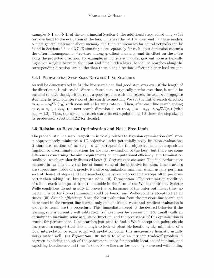
0 0.5 1 1.5
−2
0
2
4
À Á
Â
¹
distance t in line search direction
f′ (t)
5.5
6
6.5À
ÁÂ
¹
f(t)
Figure 1: Sketch: The task of a classic line search isto tune the step taken by an optimizationalgorithm along a univariate search direction.The search starts at the endpoint À of theprevious line search, at t = 0. The upperplot shows function values, the lower plotcorresponding gradients. A sequence of ex-trapolation steps Á, finds a point of positivegradient at Â. It is followed by interpolationsteps until an acceptable point ¹ is found.Points of insufficient decrease, above the linef(0) + c1tf
′(0) (white area in upper plot) areexcluded by the Armijo condition W-I, whilepoints of steep negative gradient (white areain lower plot) are excluded by the curvaturecondition W-II (the strong extension of theWolfe conditions also excludes the light greenarea in the lower plot). Point ¹ is the first tofulfill both conditions, and is thus accepted.
In essence, the same problem exists in deterministic (noise-free) optimization problems.There, providing stability is one of several tasks of the line search subroutine. It is astandard constituent of algorithms like the classic nonlinear conjugate gradient (Fletcherand Reeves, 1964) and bfgs (Broyden, 1969; Fletcher, 1970; Goldfarb, 1970; Shanno, 1970)
2

Probabilistic Line Searches
methods (Nocedal and Wright, 1999, §3).1 In the noise-free case, line searches are considereda solved problem (Nocedal and Wright, 1999, §3). But the methods used in deterministicoptimization are not stable to noise. They are easily fooled by even small disturbances,either becoming overly conservative or failing altogether. The reason for this brittleness isthat existing line searches take a sequence of hard decisions to shrink or shift the searchspace. This yields efficiency, but breaks hard in the presence of noise. Section 3 constructs aprobabilistic line search for noisy objectives, stabilizing optimization methods like the workscited above. As line searches only change the length, not the direction of a step, they couldbe used in combination with the algorithms adapting sgd’s direction, cited above. In thispaper we focus on parameter tuning of the sgd algorithm and leave other search directionsto future work.
2. Connections
2.1 Deterministic Line Searches
There is a host of existing line search variants (Nocedal and Wright, 1999, §3). In essence,though, these methods explore a univariate domain ‘to the right’ of a starting point, until an‘acceptable’ point is reached (Figure 1). More precisely, consider the problem of minimizingL(x) : RD _R, with access to ∇L(x) : RD _RD. At iteration i, some ‘outer loop’ chooses,at location xi, a search direction si ∈ RD (e.g. by the bfgs-rule, or simply si = −∇L(xi) forgradient descent). It will not be assumed that si has unit norm. The line search operatesalong the univariate domain x(t) = xi + tsi for t ∈ R+. Along this direction it collectsscalar function values and projected gradients that will be denoted f(t) = L(x(t)) andf ′(t) = sᵀi∇L(x(t)) ∈ R. Most line searches involve an initial extrapolation phase to finda point tr with f ′(tr) > 0. This is followed by a search in [0, tr], by interval nesting or byinterpolation of the collected function and gradient values, e.g. with cubic splines.2
2.1.1 The Wolfe Conditions for Termination
As the line search is only an auxiliary step within a larger iteration, it need not find an exactroot of f ′; it suffices to find a point ‘sufficiently’ close to a minimum. The Wolfe conditions(Wolfe, 1969) are a widely accepted formalization of this notion; they consider t acceptableif it fulfills
f(t) ≤ f(0) + c1tf′(0) (W-I) and f ′(t) ≥ c2f ′(0) (W-II), (2)
using two constants 0 ≤ c1 < c2 ≤ 1 chosen by the designer of the line search, not the user.W-I is the Armijo or sufficient decrease condition (Armijo, 1966). It encodes that acceptablefunctions values should lie below a linear extrapolation line of slope c1f
′(0). W-II is thecurvature condition, demanding a decrease in slope. The choice c1 = 0 accepts any valuebelow f(0), while c1 = 1 rejects all points for convex functions. For the curvature condition,
1. In these algorithms, another task of the line search is to guarantee certain properties of the surroundingestimation rule. In bfgs, e.g., it ensures positive definiteness of the estimate. This aspect will not featurehere.
2. This is the strategy in minimize.m by C. Rasmussen, which provided a model for our implementation. Atthe time of writing, it can be found at http://learning.eng.cam.ac.uk/carl/code/minimize/minimize.m
3

Mahsereci & Hennig
−101
ρ(t)
0 0.5 10
0.2
0.4
0.6
0.8
1
distance t in line search direction
pW
olfe(t)
weak
strong
0
1
pb(t)
0
1
pa(t)
ÀÁ Â ÃÄ Ï
5.5
6
6.5
f(t)
Figure 2: Sketch of a probabilistic line search. Asin Fig. 1, the algorithm performs extrapo-lation (Á,Â,Ã) and interpolation (Ä,Ï),but receives unreliable, noisy functionand gradient values. These are used toconstruct a gp posterior (top. solid pos-terior mean, thin lines at 2 standard de-viations, local pdf marginal as shading,three dashed sample paths). This impliesa bivariate Gaussian belief (§3.3) overthe validity of the weak Wolfe conditions(middle three plots. pa(t) is the marginalfor W-I, pb(t) for W-II, ρ(t) their corre-lation). Points are considered acceptableif their joint probability pWolfe(t) (bot-tom) is above a threshold (gray). An ap-proximation (§3.3.1) to the strong Wolfeconditions is shown dashed.
c2 = 0 only accepts points with f ′(t) ≥ 0; while c2 = 1 accepts any point of greater slope thanf ′(0). W-I and W-II are known as the weak form of the Wolfe conditions. The strong formreplaces W-II with |f ′(t)| ≤ c2|f ′(0)|. This guards against accepting points of low functionvalue but large positive gradient. Figure 1 shows a conceptual sketch illustrating the typicalprocess of a line search, and the weak and strong Wolfe conditions. The exposition in §3.3will initially focus on the weak conditions, which can be precisely modeled probabilistically.Section 3.3.1 then adds an approximate treatment of the strong form.
2.2 Bayesian Optimization
A recently blossoming sample-efficient approach to global optimization revolves aroundmodeling the objective f with a probability measure p(f); usually a Gaussian process (gp).Searching for extrema, evaluation points are then chosen by a utility functional u[p(f)]. Ourline search borrows the idea of a Gaussian process surrogate, and a popular acquisitionfunction, expected improvement (Jones et al., 1998). Bayesian optimization (bo) methodsare often computationally expensive, thus ill-suited for a cost-sensitive task like a linesearch. But since line searches are governors more than information extractors, the kind ofsample-efficiency expected of a Bayesian optimizer is not needed. The following sectionsdevelop a lightweight algorithm which adds only minor computational overhead to stochasticoptimization.
4
Probabilistic Line Searches
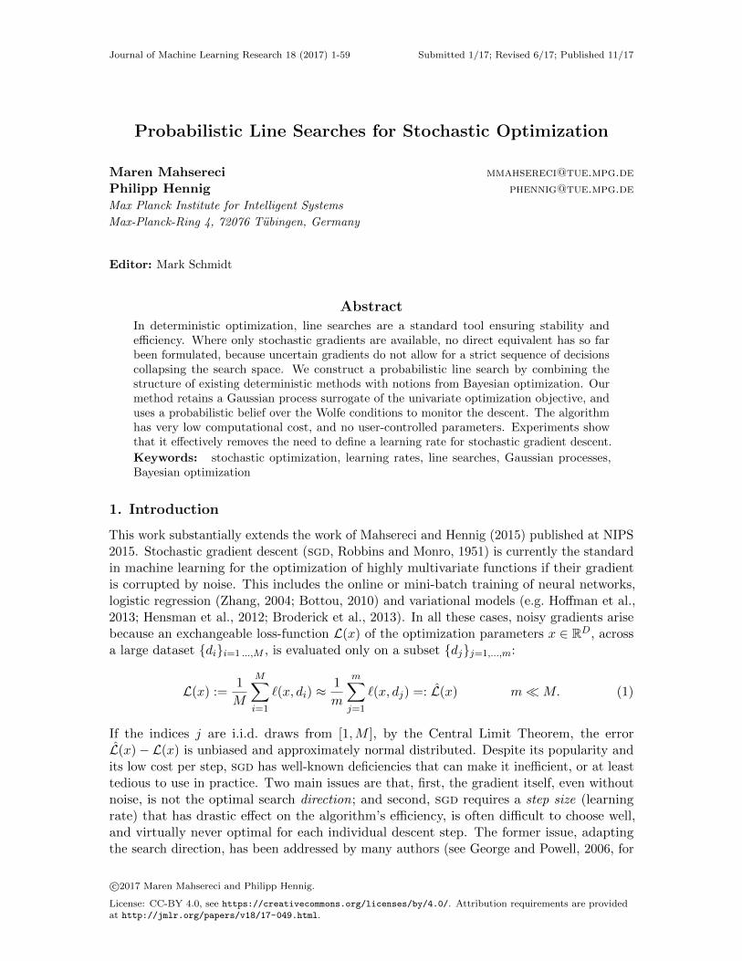
3. A Probabilistic Line Search
We now consider minimizing f(t) = L(x(t)) from Eq. 1. That is, the algorithm can accessonly noisy function values and gradients yt, y
′t at location t, with Gaussian likelihood
p(yt, y′t | f) = N
([yty′t
];
[f(t)f ′(t)
],
[σ2f 0
0 σ2f ′
]). (3)
The Gaussian form is supported by the Central Limit argument at Eq. 1. The function valueyt and the gradient y′t are assumed independent for simplicity; see §3.4 and Appendix Aregarding estimation of the variances σ2f , σ
2f ′ , and some further notes on the independence
assumption of y and y′. Each evaluation of f(t) uses a newly drawn mini-batch.Our algorithm is modeled after the classic line search routine minimize.m2 and translates
each of its building blocks one-by-one to the language of probability. The following tableillustrates these four ingredients of the probabilistic line search and their correspondingclassic parts.
building block classic probabilistic
1) 1D surrogate forobjective f(t)
piecewise cubic splines gp where the mean are piece-wise cubic splines
2) candidate selection one local minimizer of cubicsplines xor extrapolation
local minimizers of cubicsplines and extrapolation
3) choice of best candidate ——— bo acquisition function
4) acceptance criterion classic Wolfe conditions prob. Wolfe conditions
The table already motivates certain design choices, for example the particular choice ofthe gp-surrogate for f(t), which strongly resembles the classic design. Probabilistic linesearches operate in the same scheme as classic ones: 1) they construct a surrogate forthe underlying 1D-function 2) they select candidates for evaluation which can interpolatebetween datapoints or extrapolate 3) a heuristic chooses among the candidate locations andthe function is evaluated there 4) the evaluated points are checked for Wolfe-acceptance.The following sections introduce all of these building blocks with greater detail: A robust yetlightweight Gaussian process surrogate on f(t) facilitating analytic optimization (§ 3.1); asimple Bayesian optimization objective for exploration (§ 3.2); and a probabilistic formulationof the Wolfe conditions as a termination criterion (§ 3.3). Appendix D contains a detailedpseudocode of the probabilistic line search; Algorithm 1 very roughly sketches the structureof the probabilistic line search and highlights its essential ingredients.
3.1 Lightweight Gaussian Process Surrogate
We model information about the objective in a probability measure p(f). There are tworequirements on such a measure: First, it must be robust to irregularity (low and highvariability) of the objective. And second, it must allow analytic computation of discretecandidate points for evaluation, because a line search should not call yet another optimizationsubroutine itself. Both requirements are fulfilled by a once-integrated Wiener process, i.e. azero-mean Gaussian process prior p(f) = GP(f ; 0, k) with covariance function
k(t, t′) = θ2[1/3 min3(t, t′) + 1/2|t− t′|min2(t, t′)
]. (4)
5
Mahsereci & Hennig
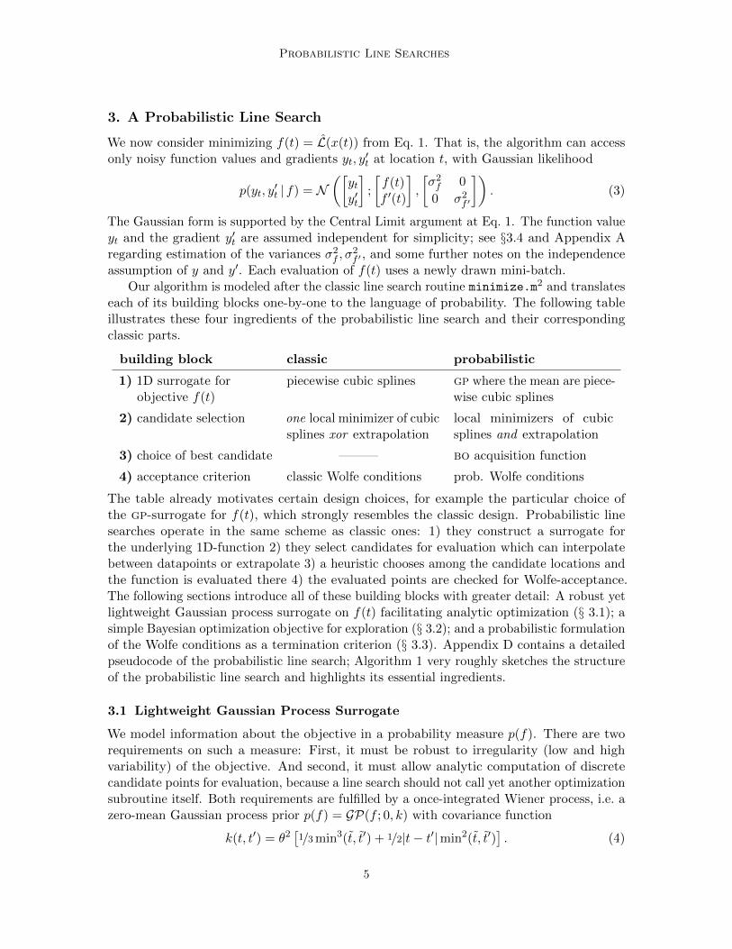
Algorithm 1 probLineSearchSketch(f , y0, y′0, σf0 , σf ′0)
GP ^initGP(y0, y′0, σf0 , σf ′0)
T, Y, Y ′^initStorage(0, y0, y′0) . for observed points
t^ 1 . scaled position of initial candidate
while budget not used and no Wolfe-point found do[y, y′] ^ f(t) . evaluate objectiveT, Y, Y ′^updateStorage(t, y, y′)GP ^updateGP(t, y, y′)PWolfe ^probWolfe(T , GP ) . compute Wolfe probability at points in T
if any PWolfe above Wolfe threshold cW thenreturn Wolfe-point
elseTcand ^computeCandidates(GP ) . positions of new candidatesEI^expectedImprovement(Tcand, GP )PW ^probWolfe(Tcand, GP )t^ where (PW � EI) is maximal . find best candidate among Tcand
end ifend while
return observed point in T with lowest gp mean since no Wolfe-point found
Here t := t+ τ and t′ := t′ + τ denote a shift by a constant τ > 0. This ensures this kernelis positive semi-definite, the precise value τ is irrelevant as the algorithm only considerspositive values of t (our implementation uses τ = 10). See §3.4 regarding the scale θ2. Withthe likelihood of Eq. 3, this prior gives rise to a gp posterior whose mean function is a cubicspline3 (Wahba, 1990). We note in passing that regression on f and f ′ from N observationsof pairs (yt, y
′t) can be formulated as a filter (Sarkka, 2013) and thus performed in O(N)
time. However, since a line search typically collects < 10 data points, generic gp inference,using a Gram matrix, has virtually the same, low cost.
Because Gaussian measures are closed under linear maps (Papoulis, 1991, §10), Eq. 4implies a Wiener process (linear spline) model on f ′:
p(f ; f ′) = GP([
ff ′
];
[00
],
[k k∂
k∂ k∂ ∂
]), (5)
3. Eq. 4 can be generalized to the ‘natural spline’, removing the need for the constant τ (Rasmussen andWilliams, 2006, §6.3.1). However, this notion is ill-defined in the case of a single observation, as in theline search.
6
Probabilistic Line Searches
0 1 2 3 4
−1
−0.5
0
0.5
t
f(t)
0 1 2 3 4
t
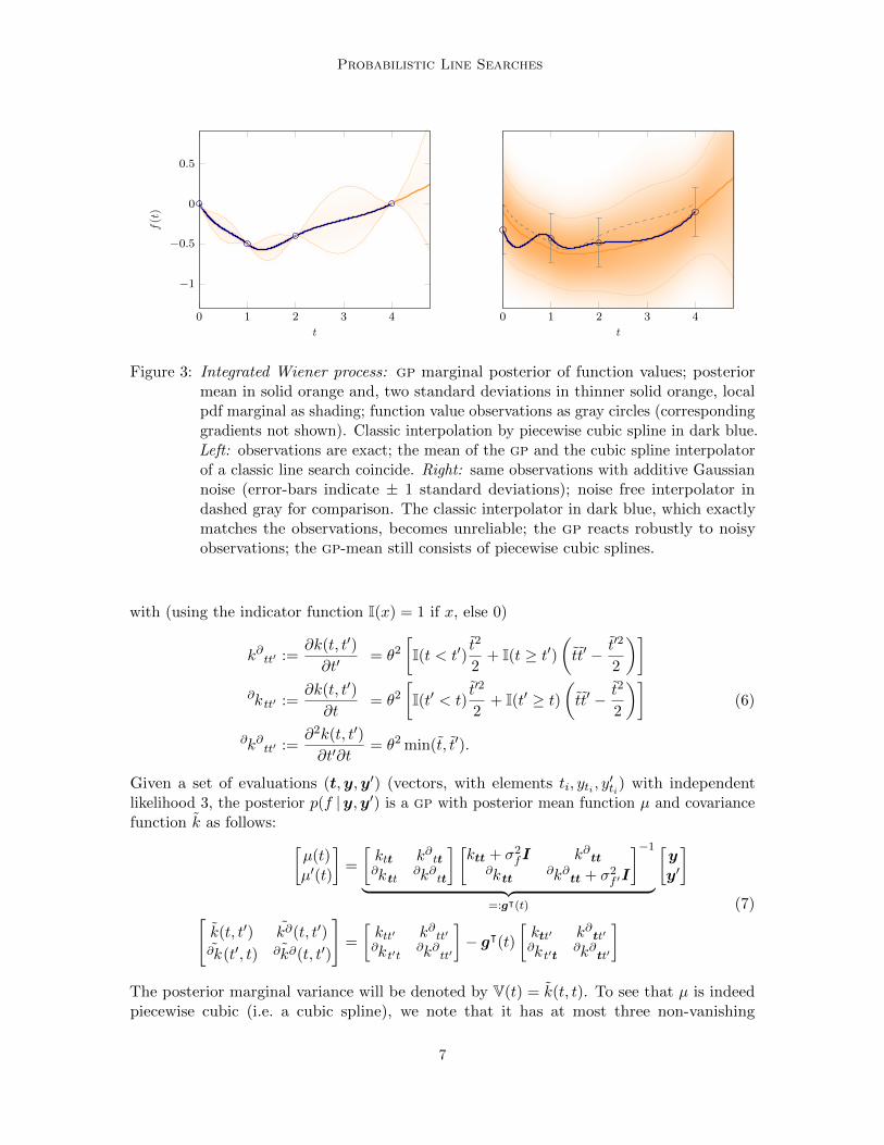
Figure 3: Integrated Wiener process: gp marginal posterior of function values; posteriormean in solid orange and, two standard deviations in thinner solid orange, localpdf marginal as shading; function value observations as gray circles (correspondinggradients not shown). Classic interpolation by piecewise cubic spline in dark blue.Left: observations are exact; the mean of the gp and the cubic spline interpolatorof a classic line search coincide. Right: same observations with additive Gaussiannoise (error-bars indicate ± 1 standard deviations); noise free interpolator indashed gray for comparison. The classic interpolator in dark blue, which exactlymatches the observations, becomes unreliable; the gp reacts robustly to noisyobservations; the gp-mean still consists of piecewise cubic splines.
with (using the indicator function I(x) = 1 if x, else 0)
k∂tt′ :=∂k(t, t′)∂t′
= θ2[I(t < t′)
t2
2+ I(t ≥ t′)
(tt′ − t′2
2
)]k∂ tt′ :=
∂k(t, t′)∂t
= θ2[I(t′ < t)
t′2
2+ I(t′ ≥ t)
(tt′ − t2
2
)](6)
k∂ ∂tt′ :=
∂2k(t, t′)∂t′∂t
= θ2 min(t, t′).
Given a set of evaluations (t,y,y′) (vectors, with elements ti, yti , y′ti) with independent
likelihood 3, the posterior p(f |y,y′) is a gp with posterior mean function µ and covariancefunction k as follows: [
µ(t)µ′(t)
]=
[ktt k∂ttk∂ tt k∂ ∂
tt
] [ktt + σ2fI k∂tt
k∂ tt k∂ ∂tt + σ2f ′I
]−1︸ ︷︷ ︸
=:gᵀ(t)
[yy′
][k(t, t′) k∂(t, t′)k∂ (t′, t) k∂ ∂(t, t′)
]=
[ktt′ k∂tt′
k∂ t′t k∂ ∂tt′
]− gᵀ(t)
[ktt′ k∂tt′
k∂ t′t k∂ ∂tt′
] (7)
The posterior marginal variance will be denoted by V(t) = k(t, t). To see that µ is indeedpiecewise cubic (i.e. a cubic spline), we note that it has at most three non-vanishing
7
Mahsereci & Hennig
derivatives4, because
k∂2tt′ :=
∂2k(t, t′)∂t2
= θ2I(t ≤ t′) k∂3tt′ :=
∂3k(t, t′)∂t3
= θ2I(t ≤ t′)(t′ − t)
k∂2 ∂tt′ :=
∂4k(t, t′)∂t2∂t′
= −θ2I(t ≤ t′) k∂3 ∂tt′ :=
∂4k(t, t′)∂t3∂t′
= 0. (8)
This piecewise cubic form of µ is crucial for our purposes: having collected N values of fand f ′, respectively, all local minima of µ can be found analytically in O(N) time in a singlesweep through the ‘cells’ ti−1 < t < ti, i = 1, . . . , N (here t0 = 0 denotes the start location,where (y0, y
′0) are ‘inherited’ from the preceding line search. For typical line searches N < 10,
c.f. §4. In each cell, µ(t) is a cubic polynomial with at most one minimum in the cell, foundby an inexpensive quadratic computation from the three scalars µ′(ti), µ′′(ti), µ′′′(ti). Thisis in contrast to other gp regression models—for example the one arising from a squaredexponential kernel—which give more involved posterior means whose local minima can befound only approximately. Another advantage of the cubic spline interpolant is that itdoes not assume the existence of higher derivatives (in contrast to the Gaussian kernel,for example), and thus reacts robustly to irregularities in the objective. In our algorithm,after each evaluation of (yN , y
′N ), we use this property to compute a short list of candidates
for the next evaluation, consisting of the ≤ N local minimizers of µ(t) and one additionalextrapolation node at tmax + α, where tmax is the currently largest evaluated t, and α is anextrapolation step size starting at α = 1 and doubled after each extrapolation step.5
A conceptual (rather than algorithmic) motivation for using the integrated Wienerprocess as surrogate for the objective, as well as for the described candidate selection, areclassic line searches. There, the 1D-objective is modeled by piecewise cubic interpolationsbetween neighboring datapoints. In a sense, this is a non-parametric approach, since anew spline is defined, when a datapoint is added. Classic line searches always only dealwith one spline at a time, since they are able to collapse all other parts of the search space.Indeed, for noise free observations, the mean of the posterior gp is identical to the classiccubic interpolations, and thus candidate locations are identical as well; this is illustrated inFigure 3. The non-parametric approach also prevents issues of over-constrained surrogatesfor more than two datapoints. For example, unless the objective is a perfect cubic function,it is impossible to fit a parametric third order polynomial to it, for more than two noisefree observations. All other variability in the objective would need to be explained awayby artificially introducing noise on the observations. An integrated Wiener process verynaturally extends its complexity with each newly added datapoint without being overlyassertive – the encoded assumption is that the objective has at least one derivative (which isalso observed in this case).
4. There is no well-defined probabilistic belief over f ′′ and higher derivatives—sample paths of the Wienerprocess are almost surely non-differentiable almost everywhere (Adler, 1981, §2.2). But µ(t) is alwaysa member of the reproducing kernel Hilbert space induced by k, thus piecewise cubic (Rasmussen andWilliams, 2006, §6.1).
5. For the integrated Wiener process and heteroscedastic noise, the variance always attains its maximumexactly at the mid-point between two evaluations; including the variance into the candidate selectionbiases the existing candidates towards the center (additional candidates might occur between evaluationswithout local minimizer, even for noise free observations/classic line searches). We did not explore thisfurther since the algorithm showed very good sample efficiency already with the adopted scheme.
8
Probabilistic Line Searches
0 0.5 1 1.5 2 2.5 3 3.5 40
0.2
0.4
0.6
0.8
1
← uEI · pWolfeuEI
↓pWolfe
↓
step size t
uEI·p
Wolfe
← local minimum extrapolation →−10
1
f′
−2−10
f
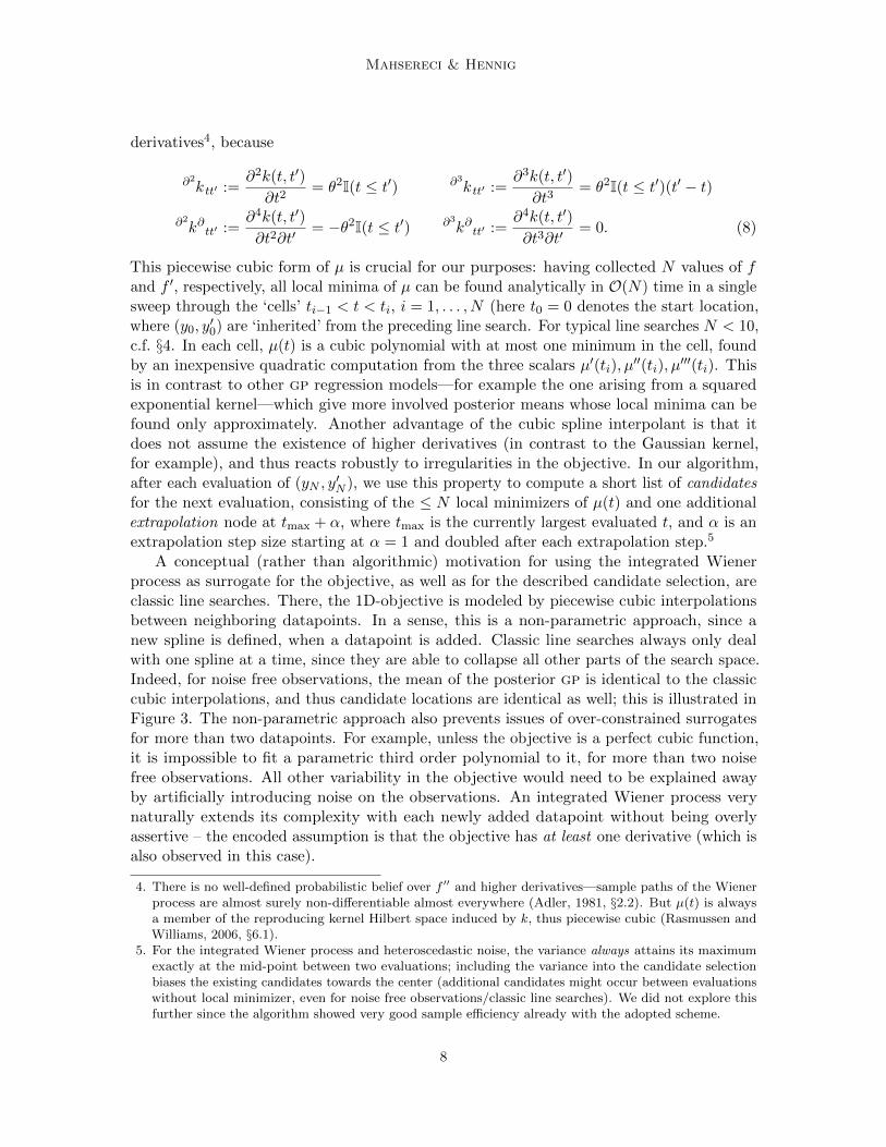
Figure 4: Candidate selection by Bayesian optimization. Top: gp marginal posterior offunction values. Posterior mean in solid orange and, two standard deviations inthinner solid orange, local pdf marginal as shading. The red and the blue pointare evaluations of the objective function, collected by the line search. Middle:gp marginal posterior of corresponding gradients. Colors same as in top plot. Inall three plots the locations of the two candidate points (§3.1) are indicated asvertical dark red lines. The left one at about tcand1 ≈ 1.54 is a local minimum ofthe posterior mean in between the red and blue point (the mean of the gradientbelief (solid orange, middle plot) crosses through zero here). The right one attcand2 = 4 is a candidate for extrapolation. Bottom: Decision criterion in arbitraryscale: The expected improvement uEI (Eq. 9) is shown in dashed light blue, theWolfe probability pWolfe (Eq. 14 and Eq. 16) in light red and their decisive productin solid dark blue. For illustrative purposes all criteria are plotted for the wholet-space. In practice solely the values at tcand1 and tcand2 are computed, compared,and the candidate with the higher value of uEI · pWolfe is chosen for evaluation. Inthis example this would be the candidate at tcand1 .
3.2 Choosing Among Candidates
The previous section described the construction of < N + 1 discrete candidate points for thenext evaluation. To decide at which of the candidate points to actually call f and f ′, we makeuse of a popular acquisition function from Bayesian optimization. Expected improvement(Jones et al., 1998) is the expected amount, under the gp surrogate, by which the functionf(t) might be smaller than a ‘current best’ value η (we set η = mini=0,...,N{µ(ti)}, where ti
9
Mahsereci & Hennig
0 1 2−1
0
1
pWolfe =0.68
0 1 2−1
0
1
pWolfe =0.08
0 1 2−1
0
1
pWolfe =0.00
W-II
W-I
← accepted−1
0
1
f′
0 0.5 1 1.5 2 2.5 3 3.5 4
−2
−1
0f
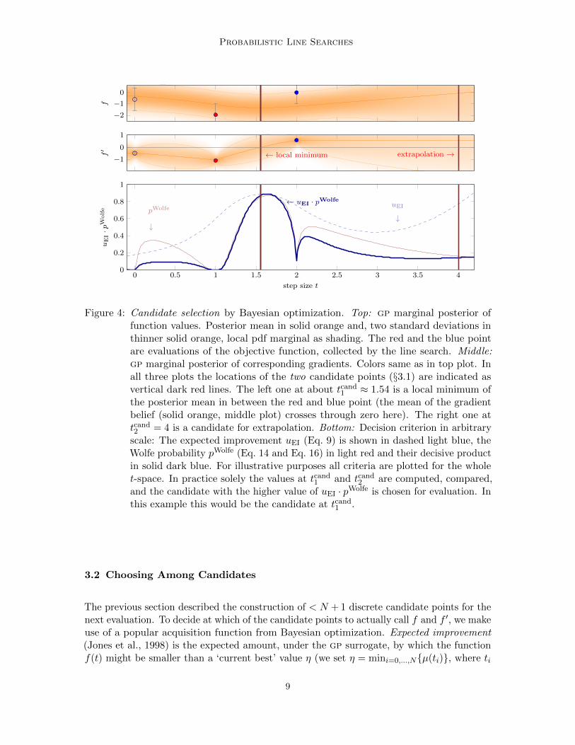
Figure 5: Acceptance procedure. Top and middle: plot and colors as in Figure 4 with anadditional ‘green’ observation. Bottom: Implied bivariate Gaussian belief overthe validity of the Wolfe conditions (Eq. 11) at the red, blue and green pointrespectively. Points are considered acceptable if their Wolfe probability pWolfe
t
is above a threshold cW = 0.3; this means that at least 30% of the orange 2DGauss density must cover greenish shaded area. Only the green point fulfills thiscondition and is therefore accepted.
0 0.5 1 1.50
1
t-constraining
pW
olfe(t)−0.2
0
0.2
f(t)
σf = 0.0028
σf ′ = 0.0049
0 2 40
1
t-extrapolation
−20
2
σf = 0.28
σf ′ = 0.0049
0 0.5 1 1.50
1
t-interpolation
−0.20
0.2
σf = 0.082
σf ′ = 0.014
0 0.5 1 1.50
1
t-immediate accept
−0.50
0.5
σf = 0.17
σf ′ = 0.012
0 0.5 1 1.50
1
t-high noise interpolation
−0.20
0.2
σf = 0.24
σf ′ = 0.011
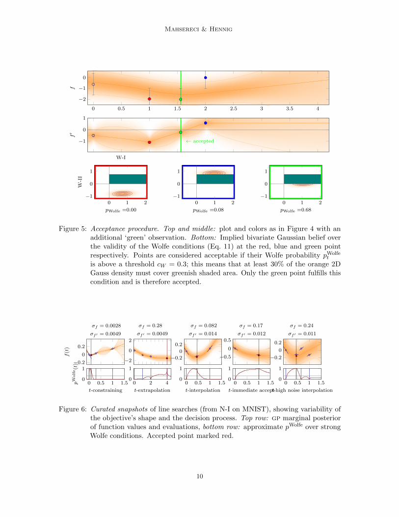
Figure 6: Curated snapshots of line searches (from N-I on MNIST), showing variability ofthe objective’s shape and the decision process. Top row: gp marginal posteriorof function values and evaluations, bottom row: approximate pWolfe over strongWolfe conditions. Accepted point marked red.
10

Probabilistic Line Searches
are observed locations),
uEI(t) = Ep(ft |y,y′)[min{0, η − f(t)}]
=η − µ(t)
2
(1 + erf
η − µ(t)√2V(t)
)+
√V(t)
2πexp
(−(η − µ(t))2
2V(t)
).
(9)
The next evaluation point is chosen as the candidate maximizing the product of Eq. 9 andWolfe probability pWolfe, which is derived in the following section. The intuition is thatpWolfe precisely encodes properties of desired points, but has poor exploration properties; uEIhas better exploration properties, but lacks the information that we are seeking a point withlow curvature; uEI thus puts weight on (by W-II) clearly ruled out points. An illustration ofthe candidate proposal and selection is shown in Figure 4.
In principle other acquisition functions (e.g. the upper-confidence bound, gp-ucb(Srinivas et al., 2010)) are possible, which might have a stronger explorative behavior;we opted for uEI since exploration is less crucial for line searches than for general boand some (e.g. gp-ucb) had one additional parameter to tune. We tracked the sampleefficiency of uEI instead and it was very good (low); the experimental Subsection 4.3 containsfurther comments and experiments on the alternative choices of uEI and pWolfe as standaloneacquisition functions; they performed equally well (in terms of loss and sample efficiency) totheir product on the tested setups.
3.3 Probabilistic Wolfe Conditions for Termination
The key observation for a probabilistic extension of the Wolfe conditions W-I and W-II isthat they are positivity constraints on two variables at, bt that are both linear projections ofthe (jointly Gaussian) variables f and f ′:
[atbt
]=
[1 c1t −1 00 −c2 0 1
]f(0)f ′(0)f(t)f ′(t)
≥ 0. (10)
The gp of Eq. (5) on f thus implies, at each value of t, a bivariate Gaussian distribution
p(at, bt) = N([atbt
];
[mat
mbt
],
[Caat CabtCbat Cbbt
]), (11)
with mat = µ(0)− µ(t) + c1tµ
′(0)
mbt = µ′(t)− c2µ′(0) (12)
and Caat = k00 + (c1t)2 k∂ ∂
00 + ktt + 2[c1t(k∂00 − k∂ 0t)− k0t]
Cbbt = c22 k∂ ∂00 − 2c2 k∂ ∂
0t + k∂ ∂tt
Cabt = Cbat = −c2(k∂00 + c1t k∂ ∂
00) + c2 k∂ 0t + k∂ t0 + c1t k∂ ∂
0t − k∂tt.(13)
The quadrant probability pWolfet = p(at > 0 ∧ bt > 0) for the Wolfe conditions to hold, is an
integral over a bivariate normal probability,
pWolfet =
∫ ∞− mat√
Caat
∫ ∞− mbt√
Cbbt
N([ab
];
[00
],
[1 ρtρt 1
])da db, (14)
11

Mahsereci & Hennig
with correlation coefficient ρt = Cabt /√Caat Cbbt . It can be computed efficiently (Drezner and
Wesolowsky, 1990), using readily available code.6 The line search computes this probabilityfor all evaluation nodes, after each evaluation. If any of the nodes fulfills the Wolfe conditionswith pWolfe
t > cW , greater than some threshold 0 < cW ≤ 1, it is accepted and returned.If several nodes simultaneously fulfill this requirement, the most recently evaluated nodeis returned; there are additional safeguards for cases where e.g. no Wolfe-point can befound, which can be deduced from the pseudo-code in Appendix D; they are similar tostandard safeguards of classic line search routines (e.g. returning the node of lowest mean).Section 3.4.1 below motivates fixing cW = 0.3. The acceptance procedure is illustrated inFigure 5.
3.3.1 Approximation for Strong Conditions:
As noted in Section 2.1.1, deterministic optimizers tend to use the strong Wolfe conditions,which use |f ′(0)| and |f ′(t)|. A precise extension of these conditions to the probabilisticsetting is numerically taxing, because the distribution over |f ′| is a non-central χ-distribution,requiring customized computations. However, a straightforward variation to 14 captures thespirit of the strong Wolfe conditions that large positive derivatives should not be accepted:Assuming f ′(0) < 0 (i.e. that the search direction is a descent direction), the strong secondWolfe condition can be written exactly as
0 ≤ bt = f ′(t)− c2f ′(0) ≤ −2c2f′(0). (15)
The value −2c2f′(0) is bounded to 95% confidence by
−2c2f′(0) . 2c2(|µ′(0)|+ 2
√V′(0)) =: b. (16)
Hence, an approximation to the strong Wolfe conditions can be reached by replacing the
infinite upper integration limit on b in Eq. 14 with (b − mbt)/√Cbbt . The effect of this
adaptation, which adds no overhead to the computation, is shown in Figure 2 as a dashedline.
3.4 Eliminating Hyper-parameters
As a black-box inner loop, the line search should not require any tuning by the user. Thepreceding section introduced six so-far undefined parameters: c1, c2, cW , θ, σf , σf ′ . We willnow show that c1, c2, cW , can be fixed by hard design decisions: θ can be eliminated bystandardizing the optimization objective within the line search; and the noise levels canbe estimated at runtime with low overhead for finite-sum objectives of the form in Eq. 1.The result is a parameter-free algorithm that effectively removes the one most problematicparameter from sgd—the learning rate.
3.4.1 Design Parameters c1, c2, cW
Our algorithm inherits the Wolfe thresholds c1 and c2 from its deterministic sibling. We setc1 = 0.05 and c2 = 0.5. This is a standard setting that yields a ‘lenient’ line search, i.e. one
6. e.g. http://www.math.wsu.edu/faculty/genz/software/matlab/bvn.m
12

Probabilistic Line Searches
that accepts most descent points. The rationale is that the stochastic aspect of sgd is notalways problematic, but can also be helpful through a kind of ‘annealing’ effect.
The acceptance threshold cW is a new design parameter arising only in the probabilisticsetting. We fix it to cW = 0.3. To motivate this value, first note that in the noise-free limit,all values 0 < cW < 1 are equivalent, because pWolfe then switches discretely between 0 and1 upon observation of the function. A back-of-the-envelope computation, assuming onlytwo evaluations at t = 0 and t = t1 and the same fixed noise level on f and f ′ (which thencancels out), shows that function values barely fulfilling the conditions, i.e. at1 = bt1 = 0, canhave pWolfe ∼ 0.2 while function values at at1 = bt1 = −ε for ε_ 0 with ‘unlucky’ evaluations(both function and gradient values one standard-deviation from true value) can achievepWolfe ∼ 0.4. The choice cW = 0.3 balances the two competing desiderata for precision andrecall. Empirically (Fig. 6), we rarely observed values of pWolfe close to this threshold. Evenat high evaluation noise, a function evaluation typically either clearly rules out the Wolfeconditions, or lifts pWolfe well above the threshold. A more in-depth analysis of c1, c2, andcW is done in the experimental Section 4.2.1.
3.4.2 Scale θ
The parameter θ of Eq. 4 simply scales the prior variance. It can be eliminated by scalingthe optimization objective: We set θ = 1 and scale yi ^ (yi−y0)/|y′0|, y
′i ^ y′i/|y′0| within the
code of the line search. This gives y(0) = 0 and y′(0) = −1, and typically ensures theobjective ranges in the single digits across 0 < t < 10, where most line searches take place.The division by |y′0| causes a non-Gaussian disturbance, but this does not seem to havenotable empirical effect.
3.4.3 Noise Scales σf , σf ′
The likelihood 3 requires standard deviations for the noise on both function values (σf )and gradients (σf ′). One could attempt to learn these across several line searches; but theresulting estimator would be biased. In exchangeable models as captured by Eq. 1, however,the variance of the loss and its gradient can be estimated locally and unbiased, directly forthe mini-batch, at low computational overhead—an approach already advocated by Schaulet al. (2013). We collect the empirical statistics
S(x) :=1
m
m∑j
`2(x, yj), and ∇S(x) :=1
m
m∑j
∇`(x, yj)�2 (17)
(where �2 denotes the element-wise square) and estimate, at the beginning of a line searchfrom xk,
σ2f =1
m− 1
(S(xk)− L(xk)
2)
and σ2f ′ = s�2iᵀ[
1
m− 1
(∇S(xk)− (∇L(xk))
�2)]. (18)
This amounts to the assumption that noise on the gradient is independent (see also Ap-pendix A). We finally scale the two empirical estimates as described in Section §3.4.2:σf ^σf/|y′(0)|, and ditto for σf ′ . The overhead of this estimation is small if the computa-tion of `(x, yj) itself is more expensive than the summation over j. In the neural network
13
Mahsereci & Hennig
examples N-I and N-II of the experimental Section 4, the additional steps added only ∼ 1%cost overhead to the evaluation of the loss. This is rather at the lower end for these models;A more general statement about memory and time requirements for neural networks can befound in Sections 3.6 and 3.7. Estimating noise separately for each input dimension capturesthe often inhomogeneous structure among gradient elements, and its effect on the noisealong the projected direction. For example, in multi-layer models, gradient noise is typicallyhigher on weights between the input and first hidden layer, hence line searches along thecorresponding directions are noisier than those along directions affecting higher-level weights.
3.4.4 Propagating Step Sizes Between Line Searches
As will be demonstrated in §4, the line search can find good step sizes even if the length ofthe direction si is mis-scaled. Since such scale issues typically persist over time, it would bewasteful to have the algorithm re-fit a good scale in each line search. Instead, we propagatestep lengths from one iteration of the search to another: We set the initial search directionto s0 = −α0∇L(x0) with some initial learning rate α0. Then, after each line search endingat xi = xi−1 + t∗si, the next search direction is set to si+1 = −αext · t∗α0∇L(xi) (withαext = 1.3). Thus, the next line search starts its extrapolation at 1.3 times the step size ofits predecessor (Section 4.2.2 for details).
3.5 Relation to Bayesian Optimization and Noise-Free Limit
The probabilistic line search algorithm is closely related to Bayesian optimization (bo) sinceit approximately minimizes a 1D-objective under potentially noisy function evaluations.It thus uses notions of bo (e.g. a gp-surrogate for the objective, and an acquisitionfunction to discriminate locations for the next evaluation of the loss), but there are somedifferences concerning the aim, requirements on computational efficiency, and terminationcondition, which are shortly discussed here: (i) Performance measure: The final performancemeasure in bo is usually the lowest found value of the objective function. Line searchesare subroutines inside of a greedy, iterative optimization machine, which usually performsseveral thousand steps (and line searches); many, very approximate steps often performsbetter than taking less, but preciser steps. (ii) Termination: The termination conditionof a line search is imposed from the outside in the form of the Wolfe conditions. StricterWolfe conditions do not usually improve the performance of the outer optimizer, thus, nomatter if a better (lower) minimum could be found, any Wolfe-point is acceptable at alltimes. (iii) Sample efficiency: Since the last evaluation from the previous line search canbe re-used in the current line search, only one additional value and gradient evaluation isenough to terminate the procedure. This ‘immediate-accept’ is the desired behavior if thelearning rate is currently well calibrated. (iv) Locations for evaluation: bo, usually calls anoptimizer to maximize some acquisition function, and the preciseness of this optimization iscrucial for performance. Line searches just need to find a Wolfe-acceptable point; classicline searches suggest that it is enough to look at plausible locations, like minimizer of alocal interpolator, or some rough extrapolation point; this inexpensive heuristic usuallyworks rather well. (v) Exploration: bo needs to solve an intricate trade-off problem inbetween exploring enough of the parameters space for possible locations of minima, andexploiting locations around them further. Since line searches are only concerned with finding
14

Probabilistic Line Searches
a Wolfe-point, they do not need to explore the parameter space of possible step sizes tothat extend; crucial features are rather the possibility to explore somewhat larger steps thanprevious ones (which is done by extrapolation-candidates), and likewise to shorted steps(which is done by interpolation-candidates).
In the limit of noise free observed gradients and function values (σf = σf ′ = 0) theprobabilistic line search behaves like its classic parent, except for very slight variations inthe candidate choice (building block 3): The gp-mean reverts to the classic interpolator; allcandidate locations are thus identical, but the probabilistic line search might propose a secondoption, since (even if there is a local minimizer) it always also proposes an extrapolationcandidate. This is illustrated in the following table.
building block classic probabilistic (noise free)
1) 1D surrogate forobjective f(t)
piecewise cubic splines gp-mean identical to classicinterpolator
2) candidate selection local minimizer of cubicsplines xor extrapolation
local minimizer of cubicsplines or extrapolation
3) choice of best candidate ——— bo acquisition function
4) acceptance criterion classic Wolfe conditions pWolfe identical to classicWolfe conditions
3.6 Computational Time Overhead
The line search routine itself has little memory and time overhead; most importantly itis independent of the dimensionality of the optimization problem. After every call of theobjective function, the gp (§3.1) needs to be updated which, at most, is at the cost ofinverting a 2N × 2N -matrix, where N usually is equal to 1, 2, or 3 but never > 10. Inaddition, the bivariate normal integral pWolfe
t of Eq. 14 needs to be computed at most Ntimes. On a laptop, one evaluation of pWolfe
t costs about 100 microseconds. For the choiceamong proposed candidates (§3.2), again at most N , for each, we need to evaluate pWolfe
t
and uEI(t) (Eq. 9) where the latter comes at the expense of evaluating two error functions.Since all of these computations have a fixed cost (in total some milliseconds on a laptop),the relative overhead becomes less the more expensive the evaluation of ∇L(x).
The largest overhead actually lies outside of the actual line search routine. In case thenoise levels σf and σf ′ are not known, we need to estimate them. The approach we took is
described in Section 3.4.3 where the variance of ∇L is estimated using the sample varianceof the mini-batch, each time the objective function is called. Since in this formulation thevariance estimation is about half as expensive as one backward pass of the net, the timeoverhead depends on the relative cost of the feed forward and backward passes (Balleset al., 2017). If forward and backward pass are the same cost, the most straightforwardimplementation of the variance estimation would make each function call < 1.3 times asexpensive. This is an upper bound and the actual cost is usually lower.7 At the same timethough, all exploratory experiments which very considerably increase the time spend when
7. It is desirable to decrease this value in the future reusing computation results or by approximation butthis is beyond this discussion.
15

Mahsereci & Hennig
using sgd with a hand tuned learning rate schedule need not be performed anymore. InSection 4.1 we will also see that sgd using the probabilistic line search often needs lessfunction evaluations to converge, which might lead to overall faster convergence in wall clocktime than classic sgd in a single run.
3.7 Memory Requirement
Vanilla sgd, at all times, keeps around the current optimization parameters x ∈ RD and thegradient vector ∇L(x) ∈ RD. In addition to this, the probabilistic line search needs to storethe estimated gradient variances Σ′(x) = (1−m)−1(∇S(x)−∇L(x)�2) (Eq. 18) of samesize. The memory requirement of sgd+probLS is thus comparable to AdaGrad or Adam.If combined with a search direction other than sgd always one additional vector of size Dneeds to be stored.
4. Experiments
This section reports on an extensive set of experiments to characterise and test the linesearch. The overall evidence from these tests is that the line search performs well and isrelatively insensitive to the choice of its internal hyper-parameters as well the mini-batchsize. We performed experiments on two multi-layer perceptrons N-I and N-II; both weretrained on two well known datasets MNIST and CIFAR-10.
• N-I: fully connected net with 1 hidden layer and 800 hidden units + biases, and 10output units, sigmoidal activation functions and a cross entropy loss. Structure withoutbiases: 784-800-10. Many authors used similar nets and reported performances.8
• N-II: fully connected net with 3 hidden layers and 10 output units, tanh-activationfunctions and a squared loss. Structure without biases: 784-1000-500-250-10. Similarnets were also used for example in Martens (2010) and Sutskever et al. (2013).
• MNIST (LeCun et al., 1998): multi-class classification task with 10 classes: hand-written digits in gray-scale of size 28× 28 (numbers ‘0’ to ’9’); training set size 60 000,test set size 10 000.
• CIFAR-10 (Krizhevsky and Hinton, 2009): multi-class classification task with 10classes: color images of natural objects (horse, dog, frog,. . . ) of size 32× 32; trainingset size 50 000, test set size 10 000; like other authors, we only used the “batch 1”sub-set of CIFAR-10 containing 10 000 training examples.
In addition we train logistic regressors with sigmoidal output (N-III) on the following binaryclassification tasks:
• Wisconsin Breast Cancer Dataset (WDBC) (Wolberg et al., 2011): binary classificationof tumors as either ‘malignant’ or ‘benign’. The set consist of 569 examples of whichwe used 169 to monitor generalization performing; thus 400 remain for the trainingset; 30 features describe for example radius, area, symmetry, et cetera. In comparison
8. http://yann.lecun.com/exdb/mnist/
16

Probabilistic Line Searches
to the other datasets and networks, this yields a very low dimensional optimizationproblem with only 30 (+1 bias) input parameters as well as just a small number ofdatapoints.
• GISETTE (Guyon et al., 2005): binary classification of the handwritten digits ‘4’ and‘9’. The original 28× 28 images are taken from the MNIST datset; then the feature setwas expanded and consists of the original normalized pixels, plus a randomly selectedsubset of products of pairs of features, which are slightly biased towards the upperpart of the image; in total there are 5000 features, instead of 784 as in the originalMNIST. The size of the training set and test set is 6000 and 1000 respectively.
• EPSILON: synthetic dataset from the PASCAL Challenge 2008 for binary classification.It consists of 400 000 training set datapoint and 100 000 test set datapoints, eachhaving 2000 features.
In the text and figures, sgd using the probabilistic line search will occasionally be denoted assgd+probLS. Section 4.1 contains experiments on the sensitivity to varying gradient noiselevels (mini-batch sizes) performed on both multi-layer perceptrons N-I and N-II, as wellas on the logistic regressor N-III. Section 4.2 discusses sensitivity to the hyper-parameterschoices introduced in Section 3.4 and Section 4.3 contains additional diagnostics on step sizestatistics. Each single experiment was performed 10 times with different random seeds thatdetermined the starting weights and the mini-batch selection and seeds were shared acrossall experiments. We report all results of the 10 instances as well as means and standarddeviations.
4.1 Varying Mini-batch Sizes
The noise level of the gradient estimate ∇L(x) and the loss L(x) is determined by themini-batch size m and ultimately there should exist an optimal m that maximizes theoptimizer’s performance in wall-clock-time. In practice of course the cost of computing∇L(x) and L(x) is not necessarily linear in m since it is upper bounded by the memorycapacity of the hardware used. We assume here that the mini-batch size is chosen by theuser; thus we test the line search with the default hyper-parameter setting (see Sections 3.4and 4.2) on four different mini-batch sizes:
• m = 10, 100, 200 and 1000 (for MNIST, CIFAR-10, and EPSILON)
• m = 10, 50, 100, and 400 (for WDBC and GISETTE)
which correspond to increasing signal-to-noise ratios. Since the training set of WDBConly consists of 400 datapoints, the run with the larges mini-batch size of 400 in fact runsfull-batch gradient descent on WDBC; this is not a problem, since—as discussed above—theprobabilistic line search can also handle noise free observations.9 We compare to sgd-runsusing a fixed step size (which is typical for these architectures) and an annealed step sizewith annealing schedule αt = α0/t. Because annealed step sizes performed much worse than
9. Since the dataset size M of WDBC is very small, we used the factor (M−m)/(mM) instead of 1/m to scalethe sample variances of Eq. 17. The former encodes sampling mini-batches B with replacement, the latterwithout replacement; for m�M both factors are nearly identical.
17

Mahsereci & Hennig
−4 −2
m:100
−4 −2
m:200
−4 −2
m:1000
−4 −2−3
−2
−1
0
log learning rate
logtest
andtrain
seterror m:10
0 1 2 3 40 1 2 3 40 1 2 3 4−3
−2
−1
0
logtrain
seterror
0 1 2 3 4
0 1 2 3 4
−1
0
# function evaluations in 104
logtest
seterror
0 1 2 3 40 1 2 3 4 0 1 2 3 4
Figure 7: Performance of N-II on MNIST for varying mini-batch sizes. Top: final logarithmictest set and train set error after 40 000 function evaluations of training versus alarge range of learning rates each for 10 different initializations. sgd-runs withfixed learning rates are shown in light blue (test set) and dark blue (train set);sgd+probLS-runs in light red (test set) and dark red (train set); means and twostandard deviations for each of the 10 runs in gray. Columns from left to rightrefer to different mini-batch sizes m of 10, 100, 200 and 1000 which correspondto decreasing relative noise in the gradient observations. Not surprisingly theperformance of sgd-runs with a fixed step size are very sensitive to the choice ofthis step size. sgd using the probabilistic line search adapts initially mis-scaledstep sizes and performs well across the whole range of initial learning rates. Middleand bottom: Evolution of the logarithmic test and train set error respectively forall sgd-runs and sgd+probLS-runs versus # function evaluations (colors as intop plot). For mini-batch sizes of m = 100, 200 and 1000 all instances of sgd usingthe probabilistic line search reach the same best test set error. Similarly a goodtrain set error is reached very fast by sgd+probLS. Only very few instances ofsgd with a fixed learning rate reach a better train set error (and this advantageusually does not translate to test set error). For very small mini-batch sizes(m = 10, first column) the line search performs poorly on this architecture, mostlikely because of the variance estimation becoming too inaccurate.
18

Probabilistic Line Searches
sgd+fixed step size, we will only report on the latter results in the plots.10 Since classicsgd without the line search needs a hand crafted learning rate we search on exhaustivelogarithmic grids of
αN-Isgd = [10−5, 5 · 10−5, 10−4, 5 · 10−4, 10−3, 5 · 10−3, 10−2, 5 · 10−2, 10−1, 5 · 10−1]
αN-IIsgd = [αN-I
sgd, 1.0, 1.5, 2.0, 2.5, 3.0, 3.5, 4.0]
αN-IIIsgd = [10−8, 10−7, 10−6, 10−5, 10−4, 10−3, 10−2, 10−1, 100, 101, 102].
We run 10 different initialization for each learning rate, each mini-batch size and each netand dataset combination (10 · 4 · (2 · 10 + 2 · 17 + 3 · 11) = 3480 runs in total) for a largeenough budget to reach convergence; and report all numbers. Then we perform the sameexperiments using the same seeds and setups with sgd using the probabilistic line searchand compare the results. For sgd+probLS, αsgd is the initial learning rate which is usedin the very first step. After that, the line search automatically adapts the learning rate, andshows no significant sensitivity to its initialization.
Results of N-I and N-II on both, MNIST and CIFAR-10 are shown in Figures 7, 14, 15,and 16; results of N-III on WDBC, GISETTE and EPSILON are shown in Figures 18, 17,and 19 respectively. All instances (sgd and sgd+probLS) get the same computationalbudget (number of mini-batch evaluations) and not the same number of optimization steps.The latter would favour the probabilistic line search since, on average, a bit more than onemini-batch is evaluated per step. Likewise, all plots show performance measure versus thenumber of mini-batch evaluations, which is proportional to the computational cost.
All plots show similar results: While classic sgd is sensitive to the learning rate choice, theline search-controlled sgd performs as good, close to, or sometimes even better than the (inpractice unknown) optimal classic sgd instance. In Figure 7, for example, sgd+probLS con-verges much faster to a good test set error than the best classic sgd instance. In allexperiments, across a reasonable range of mini-batch sizes m and of initial αsgd values,the line search quickly identified good step sizes αt, stabilized the training, and progressedefficiently, reaching test set errors similar to those reported in the literature for tuned versionsof these kind of architectures and datasets. The probabilistic line search thus effectivelyremoves the need for exploratory experiments and learning-rate tuning.
Overfitting and training error curves: The training error of sgd+probLS often plateausearlier than the one of vanilla sgd, especially for smaller mini-batch sizes. This does notseem to impair the performance of the optimizer on the test set. We did not investigatethis further, since it seemed like a nice natural annealing effect; the exact causes are unclearfor now. One explanation might be that the line search does indeed improve overfitting,since it tries to measure descent (by Wolfe conditions which rely on the noise-informed gp).This means that, if—close to a minimum—successive acceptance decisions can not identify adescent direction anymore, diffusion might set in.
4.2 Sensitivity to Design Parameters
Most, if not all, numerical methods make implicit or explicit choices about their hyper-parameters. Most of these are never seen by the user since they are either estimated at run
10. An example of annealed step size performance can be found in Mahsereci and Hennig (2015).
19

Mahsereci & Hennig
1 2 3 4
−2.5
−1.5
log reset factor θreset
log test and train set error
1 2 3 4
1.5
2.5
log reset factor θreset
average # function evaluations per line search
Figure 8: Sensitivity to varying hyper-parameters θreset. Plot and color coding as in Figure 9.Adopted parameter in dark red at θreset = 100. Resetting the gp scale occurs veryrarely. For example for θreset = 100 the reset occurred in 0.02% of all line searches.
time, or set by design to a fixed, approximately insensitive value. Well known examples arethe discount factor in ordinary differential equation solvers (Hairer et al., 1987, §2.4), or theWolfe parameters c1 and c2 of classic line searches (§3.4.1). The probabilistic line searchinherits the Wolfe parameters c1 and c2 from its classical counterpart as well as introducingtwo more: The Wolfe threshold cW and the extrapolation factor αext. cW does not appearin the classical formulation since the objective function can be evaluated exactly and theWolfe probability is binary (either fulfilled or not). While cW is thus a natural consequenceof allowing the line search to model noise explicitly, the extrapolation factor αext is theresult of the line search favoring shorter steps, which we will discuss below in more detail,but most prominently because of bias in the line search’s first gradient observation.
In the following sections we will give an intuition about the task of the most influentialdesign parameters c2, cW , and αext, discuss how they affect the probabilistic line search, andvalidate good design choices through exploring the parameter space and showing insensitivityto most of them. All experiments on hyper-parameter sensitivity were performed trainingN-II on MNIST with mini-batch size m = 200. For a full search of the parameter spacecW -c2-αext we performed 4950 runs in total with 495 different parameter combinations. Allresults are reported.
4.2.1 Wolfe II Parameter c2 and Wolfe Threshold cW
As described in Section 3.4, c2 encodes the strictness of the curvature condition W-II.Pictorially speaking, a larger c2 extends the range of acceptable gradients (green shaded arein the lower part of Figure 5) and leads to a lenient line search while a smaller value of c2shrinks this area, leading to a stricter line search. cW controls how certain we want to bethat the Wolfe conditions are actually fulfilled (pictorially, how much mass of the 2D-Gaussneed to lie in the green shaded area). In the extreme case of complete uncertainty aboutthe collected gradients and function values (roughly det[cov[a, b]]→∞) pWolfe will alwaysbe ≤ 0.25, if the strong Wolfe conditions are imposed. In the limit of certain observations(σf , σf ′ → 0) pWolfe is binary and reverts to the classic Wolfe criteria. An overly strictline search, therefore (e.g. cW = 0.99 and/ or c2 = 0.1), will still be able to optimize theobjective function well, but will waste evaluations at the expense of efficiency. Figure 10explores the c2-cW parameter space (while keeping αext fixed at 1.3). The left column showsfinal test and train set error, the right column the average number of function evaluations
20

Probabilistic Line Searches
−2.5−1.5
log test and train set error
αext =1.0
−2.5−1.5
αext =1.1
−2.5−1.5
αext =1.2
−2.5−1.5
αext =1.3
0.2 0.4 0.6 0.8
−2.5−1.5
WII parameter c2
αext =1.4
1.5
2.5
average # function evaluations per line search
αext =1.0
1.5
2.5 αext =1.1
1.5
2.5 αext =1.2
1.5
2.5 αext =1.3
0.2 0.4 0.6 0.8
1.5
2.5
WII parameter c2
αext =1.4
Figure 9: Sensitivity to varying hyper-parameters c2, and αext. Runs were performed trainingN-II on MNIST with mini-batch size m = 200. For each parameter setting 10runs with different initializations were performed. Left column: logarithmic testset error (light green) and train set error (dark green) after 40 000 functionevaluations; mean and ± two standard deviations of the 10 runs in gray. RightColumn: average number of function evaluations per line search. A low numberindicates an efficient line search procedure (perfect efficiency at 1). For mostparameter combinations this lies around ≈ 1.3− 1.5. Only at extreme parametervalues, for example αext = 1.0, which amounts to no extrapolation at all in betweensuccessive line searches, the line search performs poorer. The hyper-parametersadopted in the line search implementation are indicated as vertical dark red lineat αext = 1.3 and c2 = 0.5.
21

Mahsereci & Hennig
−2.5−1.5
log test and train set error
cW =0.01
−2.5−1.5 cW =0.10
−2.5−1.5 cW =0.20
−2.5−1.5 cW =0.30
−2.5−1.5 cW =0.40
−2.5−1.5 cW =0.50
−2.5−1.5 cW =0.60
−2.5−1.5 cW =0.70
−2.5−1.5 cW =0.80
−2.5−1.5 cW =0.90
0 0.2 0.4 0.6 0.8 1
−2.5−1.5
WII parameter c2
cW =0.99
1.5
2.5
average # function evaluations per line search
cW =0.01
1.5
2.5 cW =0.10
1.5
2.5 cW =0.20
1.5
2.5 cW =0.30
1.5
2.5 cW =0.40
1.5
2.5 cW =0.50
1.5
2.5 cW =0.60
1.5
2.5 cW =0.70
1.5
2.5 cW =0.80
1.5
2.5 cW =0.90
0.1 0.2 0.3 0.4 0.5 0.6 0.7 0.8 0.9147
WII parameter c2
cW =0.99
Figure 10: Sensitivity to varying hyper-parameters c2, and cW . Plot and color coding asin Figure 9 but this time for varying cW instead of αext. Right Column: Againa low number indicates an efficient line search procedure (perfect efficiency at1). For most parameter combinations this lies around ≈ 1.3 − 1.5. Only atextreme parameter values for example cW = 0.99, which amounts to imposingnearly absolute certainty about the Wolfe conditions, the line search becomesless efficient. Adopted parameters again in dark red at cW = 0.3 and c2 = 0.5
22
Probabilistic Line Searches
per line search, both versus different choices of Wolfe parameter c2. The left column thusshows the overall performance of the optimizer, while the right column is representative forthe computational efficiency of the line search. Intuitively, a line search which is minimallyinvasive (only corrects the learning rate, when it is really necessary) is preferred. Rows inFigure 10 show the same plot for different choices of the Wolfe threshold cW .
The effect of strict c2 can be observed clearly in Figure 10 where for smaller values ofc2 <≈ 0.2 the average number of function evaluations spend in one line search goes upslightly in comparison to looser restrictions on c2, while still a very good perfomace is reachedin terms of train and test set error. Likewise, the last row of Figure 10 for the extremevalue of cW = 0.99 (demanding 99% certainty about the validity if the Wolfe conditions),shows significant loss in computational efficiency having an average number of 7 functionevaluations per line search. Besides loosing efficiency, it is still optimizing the objective well.Lowering this threshold a bit to 90% increases the computational efficiency of the line searchto be nearly optimal again.
Ideally, we want to trade off the desiderata of being strict enough to reject too small andtoo large steps that prevent the optimizer to converge, but being lenient enough to allow allother reasonable steps, thus increasing computational efficiency. The values cW = 0.3 andc2 = 0.5, which are adopted in our current implementation are marked as dark red verticallines in Figure 10.
4.2.2 Extrapolation Factor αext
The extrapolation parameter αext, introduced in Section 3.4.4, pushes the line search to trya larger learning rate first, than the one which was accepted in the previous step. Figure 9is structured like Figure 10, but this time explores the line search sensitivity in the c2-αext
parameter space (abscissa and rows respectively) while keeping cW fixed at 0.3. Unless wechoose αext = 1.0 (no step size increase between steps) in combination with a lenient choiceof c2 the line search performs well. For now we adopt αext = 1.3 as default value whichagain is shown as dark red vertical line in Figure 9.
The introduction of αext might seem arbitrary at first, but is a necessity and well-workingfix because of a few shortcomings of the current design. First, the curvature condition W-IIis the single condition that prevents too small steps and pushes optimization progress. Onthe other hand both W-I and W-II simultaneously penalize too large steps (see Figure 1 for asketch). This is not a problem in case of deterministic observation (σf , σf ′ → 0), where W-IIundoubtedly decides if a gradient is still too negative. Unless W-II is chosen very tightly(small c2) or cW unnecessarily large (both choices, as discussed above, are undesirable),in the presence of noise, pWolfe will thus be more reliable in preventing overshooting thanpushing progress. The first row of Figure 9 illustrates this behavior, where the performancedrops somewhat if no extrapolation is done (αext = 1.0) in combination with a looser versionof W-II (larger c2).
Another factor that contributes towards accepting small rather than larger learning ratesis a bias introduced in the first observation of the line search at t = 0. Observations y′(t)that the gp gets to see are projections of the gradient sample ∇L(t) onto the search directions = −∇L(0). Since the first observations y′(0) is computed from the same mini-batch asthe search direction (not doing this would double the optimizer’s computational cost) an
23
Mahsereci & Hennig
inevitable bias is introduced of approximate size of cos−1(γ) (where γ is the expected anglebetween gradient evaluations from two independent mini-batches at t = 0). Since the scaleparameter θ of the Wiener process is implicitly set by y′(0) (§3.4.2), the gp becomes moreuncertain at unobserved points than it needs to be; or alternatively expects the 1D-gradientto cross zero at smaller steps, and thus underestimates a potential learning rate. Theposterior at observed positions is little affected. The over-estimation of θ rather pushes theposterior towards the likelihood (since there is less model to trust) and thus still gives areliable measure for f(t) and f ′(t). The effect on the Wolfe conditions is similar. With y′(0)biased towards larger values, the Wolfe conditions, which measure the drop in projectedgradient norm, are thus prone to accept larger gradients combined with smaller functionvalues, which again is met by making small steps. Ultimately though, since candidate pointsat tcand > 0 that are currently queried for acceptance, are always observed and unbiased,this can be controlled by an appropriate design of the Wolfe factor c2 (§3.4.1 and §4.2.1)and of course αext.
4.2.3 Full Hyper-Parameter Search: cW -c2-αext
An exhaustive performance evaluation on the whole cW -c2-αext-grid is shown in Appendix Cin Figures 20-24 and Figures 25-35. As discussed above, it shows the necessity of introducingthe extrapolation parameter αext and shows slightly less efficient performance for obviouslyundesirable parameter combinations. In a large volume of the parameter space, and mostimportantly in the vicinity of the chosen design parameters, the line search performance isstable and comparable to carefully hand tuned learning rates.
4.2.4 Safeguarding Mis-scaled gps: θreset
For completeness, we performed an additional experiment on the threshold parameter whichis denoted by θreset in the pseudo-code (Appendix D) and safeguards against gp mis-scaling.The introduction of noisy observations necessitates to model the variability of the 1D-function, which is described by the kernel scale parameter θ. Setting this hyper-parameteris implicitly done by scaling the observation input, assuming a similar scale than in theprevious line search (§3.4.2). If, for some reason, the previous line search accepted anunexpectedly large or small step (what this means is encoded in θreset) the gp scale θ for thenext line search is reset to an exponential running average of previous scales (αstats in thepseudo-code). This occurs very rarely (for the default value θreset = 100 the reset occurredin 0.02% of all line searches), but is necessary to safeguard against extremely mis-scaledgp’s. θreset therefore is not part of the probabilistic line search model as such, but preventsmis-scaled gps due to some unlucky observation or sudden extreme change in the learningrate. Figure 8 shows performance of the line search for θreset = 10, 100, 1000 and 10 000showing no significant performance change. We adopted θreset = 100 in our implementationsince this is the expected and desired multiplicative (inverse) factor to maximally vary thelearning rate in one single step.
4.3 Candidate Selection and Learning Rate Traces
In the current implementation of the probabilistic line search, the choice among candidatesfor evaluation is done by evaluating an acquisition function uEI(t
candi ) · pWolfe(tcandi ) at every
24
Probabilistic Line Searches
0.5 1.0 1.5 2.0 2.5
·104
−3
−2
−1
# line searches
pWolfe only
−3
−2
−1 uEI · pWolfe
−3
−2
−1
loglearn
ingrate
uEI only
−3
−2
−10
# function evaluations
logtest
andtrain
seterror
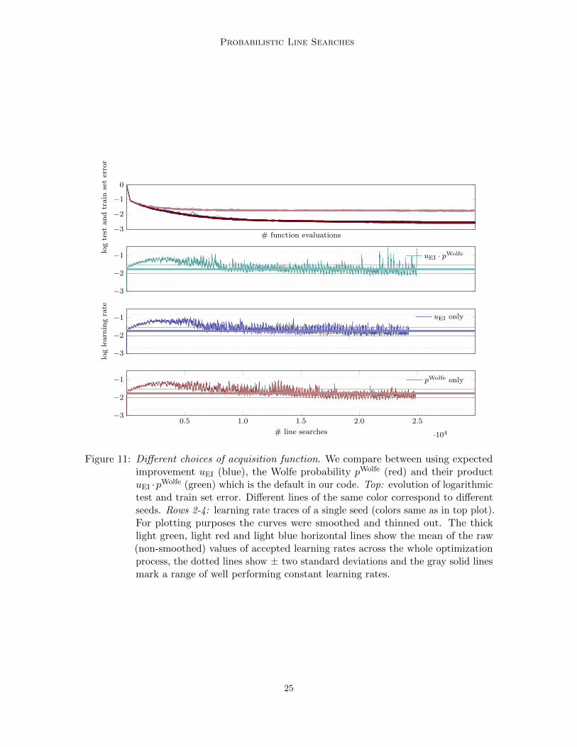
Figure 11: Different choices of acquisition function. We compare between using expectedimprovement uEI (blue), the Wolfe probability pWolfe (red) and their productuEI ·pWolfe (green) which is the default in our code. Top: evolution of logarithmictest and train set error. Different lines of the same color correspond to differentseeds. Rows 2-4: learning rate traces of a single seed (colors same as in top plot).For plotting purposes the curves were smoothed and thinned out. The thicklight green, light red and light blue horizontal lines show the mean of the raw(non-smoothed) values of accepted learning rates across the whole optimizationprocess, the dotted lines show ± two standard deviations and the gray solid linesmark a range of well performing constant learning rates.
25

Mahsereci & Hennig
−3−2−10
m =100
−3−2−10
loglearn
ingrate
m =200
0 0.5 1 1.5 2 2.5 3 3.5 4
·104
−2
0
# line searches
m =1000
Figure 12: Traces of accepted logarithmic learning rates. All runs are performed with defaultdesign parameters. Different rows show the same plot for different mini-batchsizes of m = 100, 200 and 1000; plots and smoothing as in rows 2-4 of Figure 11(details in text).
−10
1
2
3
logσf
−3.5−3−2.5−2
logσdf
0 0.2 0.4 0.6 0.8 1 1.2 1.4 1.6 1.8 2
2
4
6
# line searches in 104
average#
off-evals
m=1000
m=200
m=100
Figure 13: Traces of logarithmic noise levels σf (top), σf ′ (middle) and average numberof function evaluations per line search (bottom). Setup and smoothing as inFigure 12. Different colors correspond to different mini-batch sizes (see legend).Curves of the same color correspond to different seeds (3 shown).
26

Probabilistic Line Searches
candidate point tcandi ; then choosing the one with the highest value for evaluation of theobjective (§3.2). The Wolfe probability pWolfe actually encodes precisely what kind ofpoint we want to find and incorporates both (W-I and W-II) conditions about the functionvalue and to the gradient (§3.3). However pWolfe does not have very desirable explorationproperties. Since the uncertainty of the gp grows to ‘the right’ of the last observation, theWolfe probability quickly drops to a low, approximately constant value there (Figure 4). AlsopWolfe is partially allowing for undesirably short steps (§4.2.2). The expected improvementuEI, on the other hand, is a well studied acquisition function of Bayesian optimization tradingoff exploration and exploitation. It aims to globally find a point with a function value lowerthan a current best guess. Though this is a desirable property also for the probabilisticline search, it is lacking the information that we are seeking a point that also fulfills theW-II curvature condition. This is evident in Figure 4 where pWolfe significantly drops atpoints where the objective function is already evaluated but uEI does not. In addition, wedo not need to explore the positive t space to an extend, the expected improvement suggests,since the aim of a line search is just to find a good, acceptable point at positive t andnot the globally best one. The product of both acquisition function uEI · pWolfe is thus atrade-off between exploring enough, but still preventing too much exploitation in obviouslyundesirable regions. In practice, though, we found that all three choices ((i) uEI · pWolfe,(ii) uEI only, (iii) pWolfe only) perform comparable. The following experiments were allperformed training N-II on MNIST; only the mini-batch size might vary as indicated.
Figure 11 compares all three choices for mini-batch size m = 200 and default designparameters. The top plot shows the evolution of the logarithmic test and train set error (forplot and color description see Figure caption). All test and train set error curves respectivelybundle up (only lastly plotted clearly visible). The choice of acquisition function thus doesnot change the performance here. Rows 2-4 of Figure 11 show learning rate traces of asingle seed. All three curves show very similar global behavior. First the learning rate grows,then drops again, and finally settles around the best found constant learning rate. Thisis intriguing since on average a larger learning rate seems to be better at the beginningof the optimization process, then later dropping again to a smaller one. This might alsoexplain why sgd+probLS in the first part of the optimization progress outperforms vanillasgd (Figure 7). Runs that use just slightly larger constant learning rates than the bestperforming constant one (above the gray horizontal lines in Figure 11) were failing after afew steps. This shows that there is some non-trivial adaptation going on, not just globally,but locally at every step.
Figure 12 shows traces of accepted learning rates for different mini-batch sizes m =100, 200, 1000. Again the global behavior is qualitatively similar for all three mini-batch sizeson the given architecture. For the largest mini-batch size m = 1000 (last row of Figure 12)the probabilistic line search accepts a larger learning rate (on average and in absolute value)than for the smaller mini-batch sizes m = 100 and 200, which is in agreement with practicalexperience and theoretical findings (Hinton (2012, §4 and 7), Goodfellow et al. (2016, §9.1.3),Balles et al. (2016)).
Figure 13 shows traces of the (scaled) noise levels σf and σf ′ and the average number offunction evaluations per line search for different noise levels (m = 100, 200, 1000; same colorsshow the same setup but different seeds). The average number of function evaluations risesvery slightly to ≈ 1.5− 2 for mini-batch size m = 1000 towards the end of the optimization
27

Mahsereci & Hennig
process, in comparison to ≈ 1.5 for m = 100, 200. This seems counter intuitive in a way, butsince larger mini-batch sizes also observe smaller value and gradients (especially towards theend of the optimization process), the relative noise levels might actually be larger. (Althoughthe curves for varying m are shown versus the same abscissa, the corresponding optimizersmight be in different regions of the loss surface, especially m = 1000 probably reachesregions of smaller absolute gradients). At the start of the optimization the average numberof function evaluations is high, because the initial default learning rate is small (10−4) andthe line search extends each step multiple times.
5. Conclusion
The line search paradigm widely accepted in deterministic optimization can be extendedto noisy settings. Our design combines existing principles from the noise-free case withideas from Bayesian optimization, adapted for efficiency. We arrived at a lightweight“black-box” algorithm that exposes no parameters to the user. Empirical evaluations sofar show compatibility with the sgd search direction and viability for logistic regressionand multi-layer perceptrons. The line search effectively frees users from worries aboutthe choice of a learning rate: Any reasonable initial choice will be quickly adapted andlead to close to optimal performance. Our matlab implementation can be found at http:
//tinyurl.com/probLineSearch.
Acknowledgments
Thanks to Jonas Jaszkowic who prepared the base of the pseudo-code.
28

Probabilistic Line Searches
Appendix A. – Noise Estimation
Section 3.4.3 introduced the statistical variance estimators
Σ′(x) = (1−m)−1(∇S(x)−∇L(x)�2)
Σ(x) = (1−m)−1(S(x)− L(x)2)(19)
of the function and gradient estimate L(x) and ∇L(x) at position x. The underlyingassumption is that L(x) and ∇L(x) are distributed according to[
L(x)
∇L(x)
]∼ N
( [L(x)
∇L(x)
];
[L(x)∇L(x)
],
[Σ(x) 0D×101×D diag Σ′(x)
])(20)
which implies Eq 3[L(x)
s(x)′ · ∇L(x)
]=
[y(x)y′(x)
]∼ N
( [f(x)f ′(x)
],
[σf (x) 0
0 σf ′(x)
]). (21)
where s(x) is the possibly new search direction at x. This is an approximation since the truecovariance matrix is in general not diagonal. A better estimator for the projected gradientnoise would be (dropping x from the notation)
ηf ′ = sᵀ
[1
m− 1
1
m
m∑k=1
(∇`k −∇L)(∇`k −∇L)ᵀ
]s
=D∑
i,j=1
sisj1
m− 1
1
m
m∑k=1
(∇`ki −∇Li
)(∇`kj −∇Lj
)
=1
m− 1
D∑i,j=1
sisj
(1
m
m∑k=1
∇`ki∇`kj −∇Li∇Lj −∇Lj∇Li +∇Li∇Lj
)
=1
m− 1
1
m
m∑k=1
D∑i,j=1
si∇`ki sj∇`kj −D∑
i,j=1
sj∇Ljsi∇Li
=
1
m− 1
(1
m
m∑k=1
(s′ · ∇`k)2 − (s′ · ∇L)2
).
(22)
Comparing to σf ′ yields
ηf ′ =1
m− 1
D∑i,j=1
sisj
(1
m
m∑k=1
∇`ki∇`kj −∇Lj∇Li
)
=1
m− 1
D∑i=1
s2i
(1
m
m∑k=1
(∇`ki )2 −∇L2i
)
+1
m− 1
D∑i 6=j=1
sisj
(1
m
m∑k=1
∇`ki∇`kj −∇Lj∇Li
)
ηf ′ = σf ′ +1
m− 1
D∑i 6=j=1
sisj
(1
m
m∑k=1
∇`ki∇`kj −∇Lj∇Li
).
(23)
29

Mahsereci & Hennig
From Eq 22 we see that, in order to effectively compute ηf ′ , we need an efficient way ofcomputing the inner product (s′ · ∇`k) for all k. In addition, we need to know the searchdirection s(x) of the potential next step (if x was accepted) at the time of computingηf ′ . This is possible e.g. for the sgd search direction where s(x) = − 1
m
∑mk=1∇`k(x) but
potentially not possible or practical for arbitrary search directions. For all experiments inthis paper we used the approximate variance estimator σf ′ .
The following paragraph is concerned with the independence assumption of gradient andfunction value y and y′ (in contrast to independence among gradient elements). In general yand y′ are not independent since the algorithm draws them from the same mini-batch; thelikelihood including the correlation factor ρ reads
p(yt, y′t | f) = N
([yty′t
];
[f(t)f ′(t)
],
[σ2f ρ
ρ σ2f ′
]). (24)
The noise covariance matrix enters the gp only in the inverse of the sum with the kernelmatrix of the observations. We can compute it analytically for one datapoint at position t,since it is only a 2× 2 matrix. For ρ = 0, define:
detρ=0 := [ktt + σ2f ][ k∂ ∂tt + σ2f ′ ]− k∂tt k∂ tt
G−1ρ=0 :=
[ktt + σ2f k∂tt
k∂ tt k∂ ∂tt + σ2f ′
]−1=
1
detρ=0
[k∂ ∂
tt + σ2f ′ −k∂tt− k∂ tt ktt + σ2f
].
(25)
For ρ 6= 0 we thus get:
detρ 6=0 := [ktt + σ2f ][ k∂ ∂tt + σ2f ′ ]− [k∂tt + ρ][ k∂ tt + ρ]
= detρ=0 − ρ( k∂ tt + k∂tt)− ρ2
G−1ρ 6=0 :=
[ktt + σ2f k∂tt + ρ
k∂ tt + ρ k∂ ∂tt + σ2f ′
]−1=
1
detρ 6=0
[k∂ ∂
tt + σ2f ′ −(k∂tt + ρ)
−( k∂ tt + ρ) ktt + σ2f
]=detρ=0
detρ 6=0G−1ρ=0 −
ρ
detρ6=0
[0 11 0
] (26)
The fraction detρ=0/detρ6=0 in the first term of the last row, is a positive scalar that scalesall element of G−1ρ=0 equally (since Gρ=0 and Gρ6=0 are positive definite matrices, we knowthat detρ=0 > 0, detρ 6=0 > 0). If |ρ| is small in comparison to the determinant detρ=0, thendetρ 6=0 ≈ detρ=0 and the scaling factor is approximately one. The second term correctsoff-diagonal elements in Gρ 6=0 and is proportional to ρ; if |ρ| � detρ=0 this term is small aswell.
In might be possible to estimate ρ as well from the mini-batch in a similar style to theestimation of σf and σf ′ ; it is not clear, however, if the additional computational cost wouldjustify the improvements in the gp-inference.
30

Probabilistic Line Searches
Appendix B. – Noise Sensitivity
−4 −2 0
m:1000
−4 −2 0
m:100
−4 −2 0
−3
−2
−1
0
log learning rate
logtest
andtrain
seterror m:10
−4 −2 0
m:200
0 1 2 3 4 0 1 2 3 40 1 2 3 40 1 2 3 4
−3
−2
−1
0
logtrain
seterror
0 1 2 3 4 0 1 2 3 40 1 2 3 40 1 2 3 4
−1
0
# function evaluations in 104
logtest
seterror
Figure 14: Performance of N-I on MNIST for varying mini-batch sizes; plots and colorssame as in Figure 7 (middle plots cropped for readability).
31

Mahsereci & Hennig
−4 −2
m:1000
−4 −20
0.3
0.6
0.9
log learning rate
test
andtrain
seterror
m:10
−4 −2
m:100
−4 −2
m:200
0 0.5 10 0.5 10 0.5 10 0.5 10
0.3
0.6
0.9
train
seterror
0 0.5 10 0.5 1
0.6
0.7
0.8
0.9
# function evaluations in 104
test
seterror
0 0.5 1 0 0.5 1
Figure 15: Performance of N-II on CIFAR-10 for varying mini-batch sizes; plots and colorssame as in Figure 7, except the scaling of the y-axis which is not logarithmichere.
32
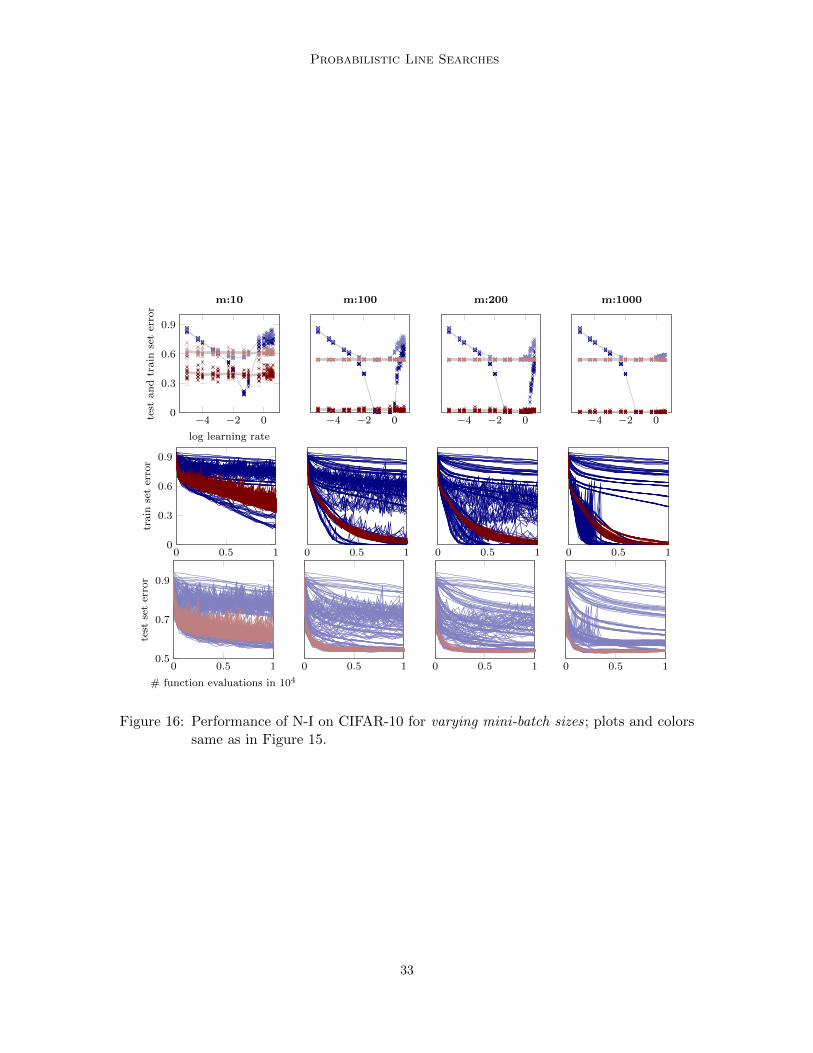
Probabilistic Line Searches
−4 −2 0
m:200
−4 −2 0
m:100
−4 −2 00
0.3
0.6
0.9
log learning rate
test
andtrain
seterror
m:10
−4 −2 0
m:1000
0 0.5 10 0.5 1 0 0.5 10 0.5 10
0.3
0.6
0.9
train
seterror
0 0.5 10.5
0.7
0.9
# function evaluations in 104
test
seterror
0 0.5 10 0.5 10 0.5 1
Figure 16: Performance of N-I on CIFAR-10 for varying mini-batch sizes; plots and colorssame as in Figure 15.
33
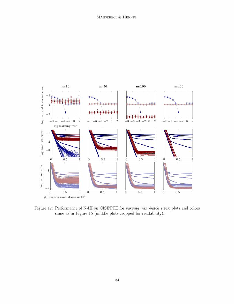
Mahsereci & Hennig
−8 −6 −4 −2 0 2
−3
−2
−1
log learning rate
logtest
andtrain
seterror m:10
−8 −6 −4 −2 0 2
m:50
−8 −6 −4 −2 0 2
m:100
−8 −6 −4 −2 0 2
m:400
0 0.5 1
−3
−2
−1
logtrain
seterror
0 0.5 1 0 0.5 1 0 0.5 1
0 0.5 1
−2
−1
# function evaluations in 104
logtest
seterror
0 0.5 1 0 0.5 1 0 0.5 1
Figure 17: Performance of N-III on GISETTE for varying mini-batch sizes ; plots and colorssame as in Figure 15 (middle plots cropped for readability).
34

Probabilistic Line Searches
−8 −6 −4 −2 0 2−1.9
−1.4
−0.9
−0.4
log learning rate
logtest
andtrain
seterror m:10
−8 −6 −4 −2 0 2
m:50
−8 −6 −4 −2 0 2
m:100
−8 −6 −4 −2 0 2
m:400
0 0.5 1−1.9
−1.4
−0.9
−0.4
logtrain
seterror
0 0.5 1 0 0.5 1 0 0.5 1
0 0.5 1−1.9
−1.4
−0.9
−0.4
# function evaluations in 105
logtest
seterror
0 0.5 1 0 0.5 1 0 0.5 1
Figure 18: Performance of N-III on WDBC for varying mini-batch sizes; plots, colors, anddescription same as in Figure 17. Remark: since the training set is of size 400, themost right column (m = 400) in fact runs full-batch gradient descent; this is nota problem, since the probabilistic line search can handle noise free observationsas well.
35

Mahsereci & Hennig
−8 −6 −4 −2 0 2
−1.2
−0.8
log learning rate
logtest
andtrain
seterror m:10
−8 −6 −4 −2 0 2
m:100
−8 −6 −4 −2 0 2
m:200
−8 −6 −4 −2 0 2
m:1000
0 10 20 30 40
−1.3
−1
−0.7
logtrain
seterror
0 1 2 3 4 0 0.5 1 1.5 2 0 0.2 0.4 0.6 0.8
0 10 20 30 40
−1.3
−1
−0.7
# function evaluations in 104
logtest
seterror
0 1 2 3 4 0 0.5 1 1.5 2 0 0.2 0.4 0.6 0.8
Figure 19: Performance of N-III on EPSILON for varying mini-batch sizes ; plots, colors, anddescription same as in Figure 17. EPSILON is the largest dataset that was usedin the experiments (400k samples); this did not seem to impair the performanceof the line search or variance estimator.
36
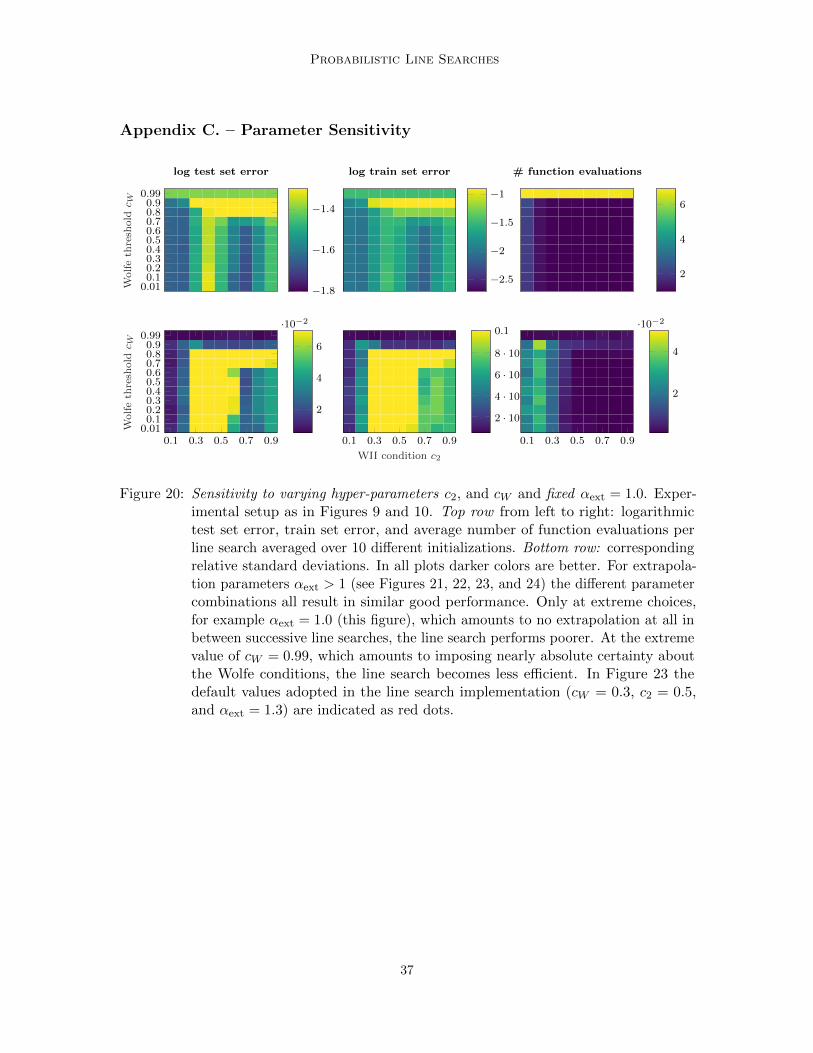
Probabilistic Line Searches
Appendix C. – Parameter Sensitivity
0.010.10.20.30.40.50.60.70.80.9
0.99
Wolfeth
resh
old
c W
log test set error
−1.8
−1.6
−1.4
log train set error
−2.5
−2
−1.5
−1
0.1 0.3 0.5 0.7 0.90.010.10.20.30.40.50.60.70.80.9
0.99
Wolfeth
resh
old
c W
2
4
6
·10−2
0.1 0.3 0.5 0.7 0.9
WII condition c2
2 · 10−2
4 · 10−2
6 · 10−2
8 · 10−2
0.1
# function evaluations
2
4
6
0.1 0.3 0.5 0.7 0.9
2
4
·10−2
Figure 20: Sensitivity to varying hyper-parameters c2, and cW and fixed αext = 1.0. Exper-imental setup as in Figures 9 and 10. Top row from left to right: logarithmictest set error, train set error, and average number of function evaluations perline search averaged over 10 different initializations. Bottom row: correspondingrelative standard deviations. In all plots darker colors are better. For extrapola-tion parameters αext > 1 (see Figures 21, 22, 23, and 24) the different parametercombinations all result in similar good performance. Only at extreme choices,for example αext = 1.0 (this figure), which amounts to no extrapolation at all inbetween successive line searches, the line search performs poorer. At the extremevalue of cW = 0.99, which amounts to imposing nearly absolute certainty aboutthe Wolfe conditions, the line search becomes less efficient. In Figure 23 thedefault values adopted in the line search implementation (cW = 0.3, c2 = 0.5,and αext = 1.3) are indicated as red dots.
37
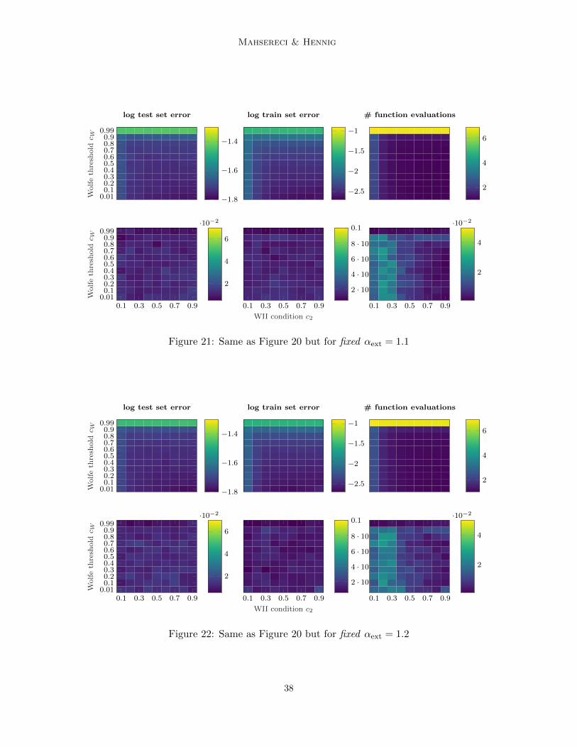
Mahsereci & Hennig
0.010.10.20.30.40.50.60.70.80.9
0.99
Wolfeth
resh
old
c W
log test set error
−1.8
−1.6
−1.4
log train set error
−2.5
−2
−1.5
−1
0.1 0.3 0.5 0.7 0.90.010.10.20.30.40.50.60.70.80.9
0.99
Wolfeth
resh
old
c W
2
4
6
·10−2
0.1 0.3 0.5 0.7 0.9
WII condition c2
2 · 10−2
4 · 10−2
6 · 10−2
8 · 10−2
0.1
# function evaluations
2
4
6
0.1 0.3 0.5 0.7 0.9
2
4
·10−2
Figure 21: Same as Figure 20 but for fixed αext = 1.1
0.010.10.20.30.40.50.60.70.80.9
0.99
Wolfeth
resh
old
c W
log test set error
−1.8
−1.6
−1.4
log train set error
−2.5
−2
−1.5
−1
0.1 0.3 0.5 0.7 0.90.010.10.20.30.40.50.60.70.80.9
0.99
Wolfeth
resh
old
c W
2
4
6
·10−2
0.1 0.3 0.5 0.7 0.9
WII condition c2
2 · 10−2
4 · 10−2
6 · 10−2
8 · 10−2
0.1
# function evaluations
2
4
6
0.1 0.3 0.5 0.7 0.9
2
4
·10−2
Figure 22: Same as Figure 20 but for fixed αext = 1.2
38

Probabilistic Line Searches
0.010.10.20.30.40.50.60.70.80.9
0.99
Wolfeth
resh
old
c W
log test set error
−1.8
−1.6
−1.4
log train set error
−2.5
−2
−1.5
−1
0.1 0.3 0.5 0.7 0.90.010.10.20.30.40.50.60.70.80.9
0.99
Wolfeth
resh
old
c W
2
4
6
·10−2
0.1 0.3 0.5 0.7 0.9
WII condition c2
2 · 10−2
4 · 10−2
6 · 10−2
8 · 10−2
0.1
# function evaluations
2
4
6
0.1 0.3 0.5 0.7 0.9
2
4
·10−2
Figure 23: Same as Figure 20 but for fixed αext = 1.3. The default values adopted in theline search implementation (cW = 0.3, c2 = 0.5, and αext = 1.3) are indicated asred dots.
0.010.10.20.30.40.50.60.70.80.9
0.99
Wolfeth
resh
old
c W
log test set error
−1.8
−1.6
−1.4
log train set error
−2.5
−2
−1.5
−1
0.1 0.3 0.5 0.7 0.90.010.10.20.30.40.50.60.70.80.9
0.99
Wolfeth
resh
old
c W
2
4
6
·10−2
0.1 0.3 0.5 0.7 0.9
WII condition c2
2 · 10−2
4 · 10−2
6 · 10−2
8 · 10−2
0.1
# function evaluations
2
4
6
0.1 0.3 0.5 0.7 0.9
2
4
·10−2
Figure 24: Same as Figure 20 but for fixed αext = 1.4
39

Mahsereci & Hennig
1.4
1.3
1.2
1.1
1
extrapolationαext
log test set error
−1.8
−1.6
−1.4
log train set error
−2.5−2−1.5−1
0.1 0.3 0.5 0.7 0.9
1.4
1.3
1.2
1.1
1
extrapolationαext
2
4
6
·10−2
0.1 0.3 0.5 0.7 0.9
WII condition c2
2 · 10−2
4 · 10−2
6 · 10−2
8 · 10−2
0.1
# function evaluations
2
4
6
0.1 0.3 0.5 0.7 0.9
2
4
·10−2
Figure 25: Sensitivity to varying hyper-parameters c2, and αext and fixed cW = 0.01. Ex-perimental setup as in Figures 9 and 10 and plots like in Figure 20. In all plotsdarker colors are better. All choices of cW result in good performance thoughvery tight choices of cW = 0.99 (Figure 35), which amounts to imposing nearlyabsolute certainty about the Wolfe conditions, are less efficient. As described inFigure 20, for a dropped extrapolation factor (αext → 1) in combination witha loose curvature condition (large c2) the line searches performs poorer (toprow, right half of columns in Figures 25–34). In Figure 28 the default valuesadopted in the line search implementation (cW = 0.3, c2 = 0.5, and αext = 1.3)are indicated as red dots.
1.4
1.3
1.2
1.1
1
extrapolationαext
log test set error
−1.8
−1.6
−1.4
log train set error
−2.5−2−1.5−1
0.1 0.3 0.5 0.7 0.9
1.4
1.3
1.2
1.1
1
extrapolationαext
2
4
6
·10−2
0.1 0.3 0.5 0.7 0.9
WII condition c2
2 · 10−2
4 · 10−2
6 · 10−2
8 · 10−2
0.1
# function evaluations
2
4
6
0.1 0.3 0.5 0.7 0.9
2
4
·10−2
Figure 26: Same as Figure 25 but for fixed cW = 0.10.
40
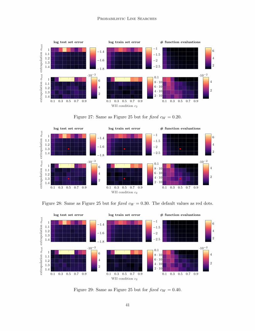
Probabilistic Line Searches
1.4
1.3
1.2
1.1
1
extrapolationαext
log test set error
−1.8
−1.6
−1.4
log train set error
−2.5−2−1.5−1
0.1 0.3 0.5 0.7 0.9
1.4
1.3
1.2
1.1
1
extrapolationαext
2
4
6
·10−2
0.1 0.3 0.5 0.7 0.9
WII condition c2
2 · 10−2
4 · 10−2
6 · 10−2
8 · 10−2
0.1
# function evaluations
2
4
6
0.1 0.3 0.5 0.7 0.9
2
4
·10−2
Figure 27: Same as Figure 25 but for fixed cW = 0.20.
1.4
1.3
1.2
1.1
1
extrapolationαext
log test set error
−1.8
−1.6
−1.4
log train set error
−2.5−2−1.5−1
0.1 0.3 0.5 0.7 0.9
1.4
1.3
1.2
1.1
1
extrapolationαext
2
4
6
·10−2
0.1 0.3 0.5 0.7 0.9
WII condition c2
2 · 10−2
4 · 10−2
6 · 10−2
8 · 10−2
0.1
# function evaluations
2
4
6
0.1 0.3 0.5 0.7 0.9
2
4
·10−2
Figure 28: Same as Figure 25 but for fixed cW = 0.30. The default values as red dots.
1.4
1.3
1.2
1.1
1
extrapolationαext
log test set error
−1.8
−1.6
−1.4
log train set error
−2.5−2−1.5−1
0.1 0.3 0.5 0.7 0.9
1.4
1.3
1.2
1.1
1
extrapolationαext
2
4
6
·10−2
0.1 0.3 0.5 0.7 0.9
WII condition c2
2 · 10−2
4 · 10−2
6 · 10−2
8 · 10−2
0.1
# function evaluations
2
4
6
0.1 0.3 0.5 0.7 0.9
2
4
·10−2
Figure 29: Same as Figure 25 but for fixed cW = 0.40.
41
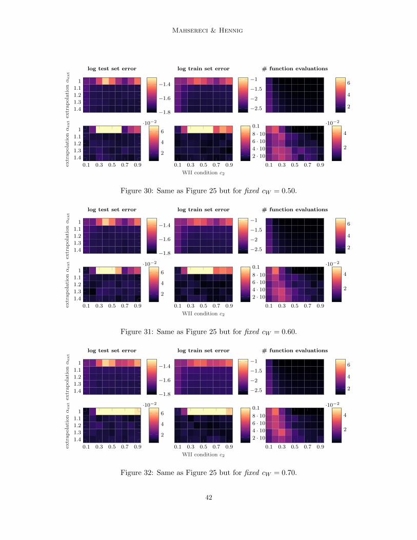
Mahsereci & Hennig
1.4
1.3
1.2
1.1
1
extrapolationαext
log test set error
−1.8
−1.6
−1.4
log train set error
−2.5−2−1.5−1
0.1 0.3 0.5 0.7 0.9
1.4
1.3
1.2
1.1
1
extrapolationαext
2
4
6
·10−2
0.1 0.3 0.5 0.7 0.9
WII condition c2
2 · 10−2
4 · 10−2
6 · 10−2
8 · 10−2
0.1
# function evaluations
2
4
6
0.1 0.3 0.5 0.7 0.9
2
4
·10−2
Figure 30: Same as Figure 25 but for fixed cW = 0.50.
1.4
1.3
1.2
1.1
1
extrapolationαext
log test set error
−1.8
−1.6
−1.4
log train set error
−2.5−2−1.5−1
0.1 0.3 0.5 0.7 0.9
1.4
1.3
1.2
1.1
1
extrapolationαext
2
4
6
·10−2
0.1 0.3 0.5 0.7 0.9
WII condition c2
2 · 10−2
4 · 10−2
6 · 10−2
8 · 10−2
0.1
# function evaluations
2
4
6
0.1 0.3 0.5 0.7 0.9
2
4
·10−2
Figure 31: Same as Figure 25 but for fixed cW = 0.60.
1.4
1.3
1.2
1.1
1
extrapolationαext
log test set error
−1.8
−1.6
−1.4
log train set error
−2.5−2−1.5−1
0.1 0.3 0.5 0.7 0.9
1.4
1.3
1.2
1.1
1
extrapolationαext
2
4
6
·10−2
0.1 0.3 0.5 0.7 0.9
WII condition c2
2 · 10−2
4 · 10−2
6 · 10−2
8 · 10−2
0.1
# function evaluations
2
4
6
0.1 0.3 0.5 0.7 0.9
2
4
·10−2
Figure 32: Same as Figure 25 but for fixed cW = 0.70.
42

Probabilistic Line Searches
1.4
1.3
1.2
1.1
1
extrapolationαext
log test set error
−1.8
−1.6
−1.4
log train set error
−2.5−2−1.5−1
0.1 0.3 0.5 0.7 0.9
1.4
1.3
1.2
1.1
1
extrapolationαext
2
4
6
·10−2
0.1 0.3 0.5 0.7 0.9
WII condition c2
2 · 10−2
4 · 10−2
6 · 10−2
8 · 10−2
0.1
# function evaluations
2
4
6
0.1 0.3 0.5 0.7 0.9
2
4
·10−2
Figure 33: Same as Figure 25 but for fixed cW = 0.80.
1.4
1.3
1.2
1.1
1
extrapolationαext
log test set error
−1.8
−1.6
−1.4
log train set error
−2.5−2−1.5−1
0.1 0.3 0.5 0.7 0.9
1.4
1.3
1.2
1.1
1
extrapolationαext
2
4
6
·10−2
0.1 0.3 0.5 0.7 0.9
WII condition c2
2 · 10−2
4 · 10−2
6 · 10−2
8 · 10−2
0.1
# function evaluations
2
4
6
0.1 0.3 0.5 0.7 0.9
2
4
·10−2
Figure 34: Same as Figure 25 but for fixed cW = 0.90.
1.4
1.3
1.2
1.1
1
extrapolationαext
log test set error
−1.8
−1.6
−1.4
log train set error
−2.5−2−1.5−1
0.1 0.3 0.5 0.7 0.9
1.4
1.3
1.2
1.1
1
extrapolationαext
2
4
6
·10−2
0.1 0.3 0.5 0.7 0.9
WII condition c2
2 · 10−2
4 · 10−2
6 · 10−2
8 · 10−2
0.1
# function evaluations
2
4
6
0.1 0.3 0.5 0.7 0.9
2
4
·10−2
Figure 35: Same as Figure 25 but for fixed cW = 0.99.
43

Mahsereci & Hennig
Appendix D. – Pseudocode
Algorithm 1 of Section 3 roughly sketches the structure of the probabilistic line searchand its main ingredients. This section provides a detailed pseudocode which can be usedfor re-implementation. It is based on the code which was used for the experiments inthis paper. A matlab implementation including a minimal example can be found at http://tinyurl.com/probLineSearch. The actual line search routine is called probLineSearchbelow and is quite short. Most of the pseudocode is occupied with comments, helper functionthat define the kernel of the gp, the gp-update or Gauss cdf and pdf which we printed herefor completeness such that a detailed re-implementation is possible. For better readabilityof the pseudocode we use the following color coding:
• blue: comments
• green: variables of the integrated Wiener process.
• red: most recently evaluated observation (noisy loss and gradient). If the line searchterminates, these will be returned as ‘accepted’.
• orange: inputs from the main solver procedure and unchanged during each line search.
Notation and operators:
operator or function definition
A�B elementwise multiplication
A�B elementwise division
A�b elementwise power of b
A′ transpose of A
A ·B scalar-scalar, scalar-matrix or matrix-matrix multiplication
A/B right matrix division, the same as A ·B−1
A\B left matrix division, the same as A−1 ·Bsign(a) sign of scalar a
erf(x) error function erf(x) = 2√π
∫ x0 e−t2dt
max(A) maximum element in A
min(A) minimum element in A
|a| absolute value of scalar a
A < B elementwise ‘less’ comparison
A ≤ B elementwise ‘less-or-equal’ comparison
A > B elementwise ‘greater’ comparison
A ≥ B elementwise ‘greater-or-equal’ comparison
[a, b, c]← f(x) function f called at x returns the values a, b and c
For better readability and to avoid confusion with transposes, we denote derivatives forexample as dy and df (instead of y′ and f ′ as in the main text).
44

Probabilistic Line Searches
1: function SGDSolver(f)2: I f – function handle to objective. Usage: [y, dy,Σf ,Σdf ] ^ f(x).
3:
4: I initial weights5: x^initial weights6:
7: I initial step size (rather small to avoid over-shooting in very first step)8: α^ e.g. ≈ 10−4
9: αstats ^α10:
11: I initial function evaluation at x12: [y, dy,Σf ,Σdf ] ^ f(x)13:
14: I initial search direction15: d^−dy16:
17: I loop over line searches18: while budget not used do19:
20: I line search finds step size21: [α, αstats, x, y, dy,Σf ,Σdf ] ^probLineSearch(x, d, y, dy,Σf ,Σdf , α, αstats, f)22:
23: I set new search direction24: d^−dy25: end while26:
27: return x28: end function
1: function probLineSearch(x0, d, f0, df0,Σf0 ,Σdf0 , α0, αstats, f)2: I x0 – current weights [D × 1]3: I f – function handle to objective.4: I5: I d – search direction [D × 1] (does not need to be normalized)6: I f0 – function value at start, f0 = f(x0)7: I df0 – gradient at start, df0 = ∇f(x0) [D × 1]8: IΣf0 – sample variance of f09: IΣdf0 – sample variances of df0, [D × 1]
10: I α0 – initial step size11:
12: I set maximum # of f evaluations per line search13: L ^ 6
45

Mahsereci & Hennig
14: I scaling and noise level of gp15: β^ |d′ · Σdf0 | . scale factor16: σf ^
√Σf0/(α0 · β) . scaled sample variance of f0
17: σdf ^√
((d�2)′ · Σdf0)/β . scaled and projected sample variances of df018:
19: I initialize counter and non-fixed parameters20: N ^ 1 . size of gp= 2 ·N21: text ^ 1 . scaled step size for extrapolation22: tt^ 1 . scaled position of first function evaluation23:
24: I initialize storage for gp. Dynamic arrays of maximum size [L+ 1× 1]25: T ^[0] . scaled positions along search direction26: Y ^[0] . scaled function values at T27: dY ^[(df0
′ · d)/β] . scaled projected gradients at T28:
29: I initialize gp with observation at start30: [G,A] ^updateGP(T , Y , dY ,N, σf , σdf )31:
32: I loop until budged is used or acceptable point is found33: for N from 2 to L + 1 do34:
35: I evaluate objective function at tt.36: [y, dy,Σf ,Σdf , T , Y , dY ,N ] ^evaluateObjective(tt, x0, α0, d, T , Y , dY ,N, β, f)37:
38: I update the gp which is now of size 2 ·N .39: [G,A] ^updateGP(T , Y , dY ,N, σf , σdf )40:
41: I initialize storage for candidates. Dynamic arrays of maximum size [N × 1].42: Tcand ^[ ] . scaled position of candidates43: Mcand ^[ ] . gp mean of candidates44: Scand ^[ ] . gp standard deviation of candidates45:
46: I current point is above the Wolfe threshold? If yes, accept point and return.47: if probWolfe(tt, T ,A,G) then48: output^rescaleOutput(x0, f0, α0, d, tt, y, dy,Σf ,Σdf , β)49: return output50: end if51:
52: IWolfe conditions not satisfied at this point.53: I find suitable candidates for next evaluation.54:
55: I gp mean of function values and corresponding gradients at points in T .56: M ^ map function m( , T , A) over T57: dM ^ map function d1m( , T , A) over T
46

Probabilistic Line Searches
58: I candidates 1: local minima of gp mean.59: Tsorted ^ sort T in ascending order60: TWolfes ^[ ] . prepare list of acceptable points61:
62: I iterate through all N − 1 cells, compute locations of local minima.63: for n from 1 to N − 1 do64: Tn ^ value of Tsorted at n65: Tn+1 ^ value of Tsorted at n+ 166:
67: I add a little offset for numerical stability68: trep ^Tn + 10−6 · (Tn+1 − Tn)69:
70: I compute location of cubic minimum in nth cell71: tcubMin ^cubicMinimum(trep, T , A,N)72:
73: I add point to candidate list if minimum lies in between Tn and Tn+1
74: if tcubMin > Tn and tcubMin < Tn+1 then75: if (not isnanOrIsinf(tcubMin)) and (tcubMin > 0) then76: Tcand ^ append tcubMin
77: Mcand ^ append m(tcubMin, T , A)78: Scand ^ append V(tcubMin, T ,G)79: end if80: else81:
82: I most likely uphill? If yes, break.83: if n = 1 and d1m(0, T , A) > 0 then84: r^ 0.0185: tt^ r · (Tn + Tn+1)86:
87: I evaluate objective function at tt and return.88: [y, dy,Σf ,Σdf , T , Y , dY ,N ] ^evaluateObjective(tt, x0, α0, d, T , Y , dY ,N, β, f)89:
90: output^rescaleOutput(x0, f0, α0, d, tt, y, dy,Σf ,Σdf , β)91: return output92: end if93: end if94:
95: I check whether there is an acceptable point among the old evaluations96: if n > 1 and probWolfe(Tn, T , A,G) then97: TWolfes ^ append Tn98: end if99: end for100:
101: I check if acceptable points exists and return102: if TWolfes is not empty then
47

Mahsereci & Hennig
103: I if last evaluated point is among acceptable ones, return it.104: if tt in TWolfes then105: output^rescaleOutput(x0, f0, α0, d, tt, y, dy,Σf ,Σdf , β)106: return output107: end if108:
109: I else, choose the one with the lowest gp mean and re-evaluate its gradient.110: MWolfes ^ map m( , T , A) over TWolfes
111: tt^ value of TWolfes at index of min(MWolfes)112:
113: I evaluate objective function at tt.114: [y, dy,Σf ,Σdf , T , Y , dY ,N ] ^evaluateObjective(tt, x0, α0, d, T , Y , dY ,N, β, f)115:
116: output^rescaleOutput(x0, f0, α0, d, tt, y, dy,Σf ,Σdf , β)117: return output118: end if119:
120: I candidates 2: one extrapolation step121: Tcand ^ append max(T ) + text122: Mcand ^ append m(max(T ) + text, T , A)
123: Scand ^ append V(max(T ) + text, T ,G)12
124:
125: I find minimal mean among M .126: µEI ^ minimal value of M127:
128: I compute expected improvement and Wolfe probabilities at Tcand129: EIcand ^expectedImprovement(Mcand, Scand, µEI)130: PWcand ^ map probWolfe( , T , A,G) over Tcand131:
132: I choose point among candidates that maximizes EIcand ∧ PWcand
133: ibestCand ^ index of max(EIcand � PWcand)134: ttbestCand ^ value of Tcand at ibestCand
135:
136: I extend extrapolation step if necessary137: if ttbestCand is equal to tt+ text then138: text ^ 2 · text139: end if140:
141: I set location for next evaluation142: tt^ ttbestCand
143: end for144:
145: I limit reached: evaluate a final time and return the point with lowest gp mean146: [y, dy,Σf ,Σdf , T , Y , dY ,N ] ^evaluateObjective(tt, x0, α0, d, T , Y , dY ,N, β, f)
48
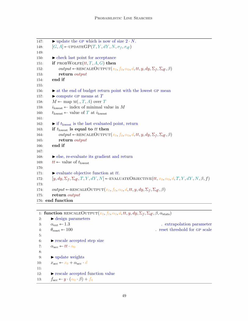
Probabilistic Line Searches
147: I update the gp which is now of size 2 ·N .148: [G,A] ^updateGP(T , Y , dY ,N, σf , σdf )149:
150: I check last point for acceptance151: if probWolfe(tt, T ,A,G) then152: output^rescaleOutput(x0, f0, α0, d, tt, y, dy,Σf ,Σdf , β)153: return output154: end if155:
156: I at the end of budget return point with the lowest gp mean157: I compute gp means at T158: M ^ map m( , T , A) over T159: ilowest ^ index of minimal value in M160: tlowest ^ value of T at ilowest161:
162: I if tlowest is the last evaluated point, return163: if tlowest is equal to tt then164: output^rescaleOutput(x0, f0, α0, d, tt, y, dy,Σf ,Σdf , β)165: return output166: end if167:
168: I else, re-evaluate its gradient and return169: tt^ value of tlowest170:
171: I evaluate objective function at tt.172: [y, dy,Σf ,Σdf , T , Y , dY ,N ] ^evaluateObjective(tt, x0, α0, d, T , Y , dY ,N, β, f)173:
174: output^rescaleOutput(x0, f0, α0, d, tt, y, dy,Σf ,Σdf , β)175: return output176: end function
1: function rescaleOutput(x0, f0, α0, d, tt, y, dy,Σf ,Σdf , β, αstats)2: I design parameters3: αext ^ 1.3 . extrapolation parameter4: θreset ^ 100 . reset threshold for gp scale5:
6: I rescale accepted step size7: αacc ^ tt · α0
8:
9: I update weights10: xacc ^x0 + αacc · d11:
12: I rescale accepted function value13: facc ^ y · (α0 · β) + f0
49

Mahsereci & Hennig
14: I accepted gradient15: dfacc ^ dy16:
17: I sample variance of facc18: Σfacc ^ Σf
19:
20: I sample variances of dfacc21: Σdfacc ^ Σdf
22:
23: I update exponential running average of scalings24: γ^ 0.9525: αstats ^ γ · αstats + (1− γ) · αacc
26:
27: I next initial step size28: αnext ^αacc · αext
29:
30: I if new gp scaling is drastically different than previous ones reset it.31: if (αnext < αstats/θreset) or (αnext > αstats · θreset) then32: αnext ^αstats
33: end if34:
35: I compressed output for readability of pseudocode36: output^[αnext, αstats, xacc, facc, dfacc,Σfacc ,Σdfacc ]37:
38: return output39: end function
1: function evaluateObjective(tt, x0, α0, d, T , Y , dY ,N, β, f)2: I evaluate objective function at tt3: [y, dy,Σf ,Σdf ] ^ f(x0 + tt · α0 · d)4:
5: I scale output6: y^(y − f0)/(α0 · β)7: dy^(dy′ · d)/β8:
9: I storage
10: T ^ append tt11: Y ^ append y12: dY ^ append dy13: N ^N + 114:
15: return [y, dy,Σf ,Σdf , T, Y, dY,N ]16: end function
50

Probabilistic Line Searches
1: function cubicMinimum(t, T ,A,N)2: I compute necessary derivatives of gp mean at t3: d1mt ^d1m(t, T ,A)4: d2mt ^d2m(t, T ,A)5: d3mt ^d3m(t, T ,A,N)6: a^ 0.5 · d3mt
7: b^ d2mt − t · d3mt
8: c^ d1mt − d2mt · t+ 0.5 · d3mt · t29:
10: I third derivative is almost zero → essentially a quadratic, single extremum11: if |d3mt| < 1−9 then12: tcubMin ^−(d1mt − t · d2mt)/d2mt
13: return tcubMin
14: end if15:
16: I roots are complex, no extremum17: λ^ b2 − 4 · a · c18: if λ < 0 then19: tcubMin ^ +∞20: return tcubMin
21: end if22:
23: I compute the two possible roots24: LR^(−b− sign(a) ·
√λ)/(2 · a) . left root
25: RR^(−b+ sign(a) ·√λ)/(2 · a) . right root
26:
27: I calculate the two values of the cubic at those points (up to a constant)28: dtL ^LR− t . distance to left root29: dtR ^RR− t . distance to right root30: CVL ^ d1mt · dtL + 0.5 · d2mt · dt2L + (d3mt · dt3L)/6 . left cubic value31: CVR ^ d1mt · dtR + 0.5 · d2mt · dt2R + (d3mt · dt3R)/6 . right cubic value32:
33: I find the minimum and return it.34: if CVL < CVR then35: tcubMin ^LR36: else37: tcubMin ^RR38: end if39:
40: return tcubMin
41:
42: end function
51

Mahsereci & Hennig
1: function updateGP(T , Y , dY ,N, σf , σdf )2: I initialize kernel matrices3: kTT ^[N ×N ] matrix with zeros . covariance of function values4: kdTT ^[N ×N ] matrix with zeros . covariance of function values and gradients5: dkdTT ^[N ×N ] matrix with zeros . covariance of gradients6:
7: I fill kernel matrices8: for i = 1 to N do9: for j = 1 to N do
10: kTT (i, j) ^k(T (i), T (j))11: kdTT (i, j) ^kd(T (i), T (j))12: dkdTT (i, j) ^dkd(T (i), T (j))13: end for14: end for15:
16: I build diagonal covariance matrix of Gaussian likelihood [2N × 2N ].
17: Λ ^[diag(σf
2)N×N 0N×N0N×N diag(σdf
2)N×N
]18:
19: G^(
kTT kdTTkd′TT dkdTT
)+ Λ . [2N × 2N ] matrix
20:
21: I residual between observed and predicted data
22: ∆ ^(
YdY
). [2N × 1] vector
23:
24: I compute weighted observations A.25: A^G\∆ . [2N × 1] vector26:
27: return [G,A]28:
29: end function
52

Probabilistic Line Searches
1: function m(t, T ,A)2: I posterior mean at t
3: return [k(t, T ′), kd(t, T ′)] ·A4: end function5:
6: function d1m(t, T ,A)7: I first derivative of mean at t8: return [dk(t, T ′), dkd(t, T ′)] ·A9: end function
10:
11: function d2m(t, T ,A)12: I second derivative of mean at t13: return [ddk(t, T ′), ddkd(t, T ′)] ·A14: end function15:
16: function d3m(t, T ,A,N)17: I third derivative of mean at t18: return [dddk(t, T ′), zeros(1, N)] ·A19: end function20:
21: function V(t, T ,G)22: I posterior variance of function values at t23: return k(t, t)−[k((t, T ′), kd(t, T ′)] · (G\[k(t, T ′), kd(t, T ′)]′)24: end function25:
26: function Vd(t, T ,G)27: I posterior variance of function values and derivatives at t28: return kd(t, t)−[k(t, T ′), kd(t, T ′)] · (G\[dk(t, T ′), dkd(t, T ′)]′)29: end function30:
31: function dVd(t, T ,G)32: I posterior variance of derivatives at t33: return dkd(t, t)−[dk(t, T ′), dkd(t, T ′)] · (G\[dk(t, T ′), dkd(t, T ′)]′)34: end function35:
36: function V0f(t, T ,G)37: I posterior covariances of function values at t = 0 and t38: return k(0, t)−[k(0, T ′), kd(0, T ′)] · (G\[k(t, T ′), kd(t, T ′)]′)39: end function40:
41: function Vd0f(t, T ,G)42: I posterior covariance of gradient and function value at t = 0 and t respectively43: return dk(0, t)−[dk(0, T ′), dkd(0, T ′)] · (G\[k(t, T ′), kd(t, T ′)]′)44: end function
53

Mahsereci & Hennig
45: function V0df(t, T ,G)46: I posterior covariance of function value and gradient at t = 0 and t respectively47: return kd(0, t) −[k(0, T ′), kd(0, T ′)] · (G\[dk(t, T ′), dkd(t, T ′)]′)48: end function49:
50: function Vd0df(t, T ,G)51: I same as V0f( ) but for gradients52: return dkd(0, t)−[dk(0, T ′), dkd(0, T ′)] · (G\[dk(t, T ′), dkd(t, T ′)]′)53: end function
1: ————————————————–2: I all following procedures use the same design parameter:3: τ ^ 104: ————————————————–5: function k(a, b)6: IWiener kernel integrated once in each argument7: return 1/3�min(a+ τ , b+ τ)�3 + 0.5� |a− b| �min(a+ τ , b+ τ)�2
8: end function9:
10: function kd(a, b)11: IWiener kernel integrated in first argument12: return 0.5� (a < b)� (a+ τ)�2 + (a ≥ b)�
((a+ τ) · (b+ τ)− 0.5� (b+ τ)�2
)13: end function14:
15: function dk(a, b)16: IWiener kernel integrated in second argument17: return 0.5� (a > b)� (b+ τ)�2 + (a ≤ b)� ((a+ τ) · (b+ τ)− 0.5� (a+ τ)�2)18: end function19:
20: function dkd(a, b)21: IWiener kernel22: return min(a+ τ , b+ τ)23: end function24:
25: function ddk(a, b)26: IWiener kernel integrated in second argument and 1x derived in first argument27: return (a ≤ b)� (b− a)28: end function29:
30: function ddkd(a, b)31: IWiener kernel 1x derived in first argument32: return (a ≤ b)33: end function
54

Probabilistic Line Searches
34: function dddk(a, b)35: IWiener kernel 2x derived in first argument and integrated in second argument36: return −(a ≤ b)37: end function
1: function probWolfe(t, T ,A,G)2: I design parameters3: c1 ^ 0.05 . constant for Armijo condition4: c2 ^ 0.5 . constant for curvature condition5: cW ^ 0.3 . threshold for Wolfe probability6:
7: I mean and covariance values at start position (t = 0)8: m0 ^ m(0, T , A)9: dm0 ^d1m(0, T , A)
10: V0 ^ V(0, T ,G)11: V d0 ^ Vd(0, T ,G)12: dV d0 ^ dVd(0, T ,G)13:
14: I marginal mean and variance for Armijo condition15: ma ^m0−m(t, T ,A)+c1 · t · dm0
16: Vaa ^V0 + (c1 · t)2 · dV d0+V(t)+2 · (c1 · t · (V d0−Vd0f(t))−V0f(t))17:
18: I marginal mean and variance for curvature condition19: mb ^d1m(t)−c2 · dm0
20: Vbb ^ c22 · dV d0 − 2 · c2 ·Vd0df(t)+dVd(t)
21:
22: I covariance between conditions23: Vab ^−c2 · (V d0 + c1 · t · dV d0) + c2 ·Vd0f(t)+V0df(t)+c1 · t·Vd0df(t)−Vd(t)24:
25: I extremely small variances → very certain (deterministic evaluation)26: if Vaa ≤ 10−9 and Vbb ≤ 10−9 then27: pWolfe ^(ma ≥ 0) · (mb ≥ 0)28:
29: I accept?30: pacc ^ pWolfe > cW31: return pacc32: end if33:
34: I zero or negative variances (maybe something went wrong?)35: if Vaa ≤ 0 or Vbb ≤ 0 then36: return 037: end if
55

Mahsereci & Hennig
38: I noisy case (everything is alright)39: I correlation40: ρ^Vab/
√Vaa · Vbb
41:
42: I lower and upper integral limits for Armijo condition43: lowa ^−ma/
√Vaa
44: upa ^ +∞45:
46: I lower and upper integral limits for curvature condition47: lowb ^−mb/
√Vbb
48: upb ^(2 · c2 ·
(|dm0|+ 2 ·
√dV d0
)−mb
)/√Vbb
49:
50: I compute Wolfe probability51: pWolfe ^bvn(lowa, upa, lowb, upb, ρ)52:
53: I accept?54: pacc ^ pWolfe > cW55: return pacc56:
57:
The function bvn(lowa, upa, lowb, upb, ρ) evaluates the 2D-integral∫ upa
lowa
∫ upb
lowb
N([ab
];
[00
],
[1 ρρ 1
])dadb.
58:
59: end function
1: function gaussCDF(z)2: I Gauss cumulative density function3: return 0.5�
(1 + erf(z/
√2))
4: end function5:
6: function gaussPDF(z)7: I Gauss probability density function8: return exp
(−0.5� z�2
)�√
2π9: end function
10:
11: function expectedImprovement(m, s, η)12: I Jones et al. (1998)13: return (η −m)�gaussCDF((η −m)� s) +s�gaussPDF((η −m)� s)14: end function
56

Probabilistic Line Searches
References
R.J. Adler. The Geometry of Random Fields. Wiley, 1981.
S.-I. Amari, H. Park, and K. Fukumizu. Adaptive method of realizing natural gradient learning formultilayer perceptrons. Neural Computation, 12(6):1399–1409, 2000.
M. Andrychowicz, M. Denil, S. Gomez-Colmenarejo, M.W. Hoffman, D. Pfau, T. Schaul, and Nandode Freitas. Learning to learn by gradient descent by gradient descent. CoRR, abs/1606.04474,2016. URL http://arxiv.org/abs/1606.04474.
L. Armijo. Minimization of functions having Lipschitz continuous first partial derivatives. PacificJournal of Mathematics, 16(1):1–3, 1966.
L. Balles, J. Romero, and P. Hennig. Coupling Adaptive Batch Sizes with Learning Rates. ArXive-prints, December 2016.
L. Balles, M. Mahsereci, and P. Hennig. Automating stochastic optimization with gradient varianceestimates. ICML AutoML Workshop, 2017.
L. Bottou. Large-scale machine learning with stochastic gradient descent. In Proceedings of the 19thInt. Conf. on Computational Statistic (COMPSTAT), pages 177–186. Springer, 2010.
T. Broderick, N. Boyd, A. Wibisono, A.C. Wilson, and M.I. Jordan. Streaming variational Bayes. InAdvances in Neural Information Processing Systems (NIPS 26), pages 1727–1735, 2013.
C.G. Broyden. A new double-rank minimization algorithm. Notices of the AMS, 16(4):670, 1969.
Z. Drezner and G.O. Wesolowsky. On the computation of the bivariate normal integral. Journal ofStatistical Computation and Simulation, 35(1-2):101–107, 1990.
J. Duchi, E. Hazan, and Y. Singer. Adaptive subgradient methods for online learning and stochasticoptimization. Journal of Machine Learning Research, 12:2121–2159, 2011.
R. Fletcher. A new approach to variable metric algorithms. The Computer Journal, 13(3):317, 1970.
R. Fletcher and C.M. Reeves. Function minimization by conjugate gradients. The Computer Journal,7(2):149–154, 1964.
A.P. George and W.B. Powell. Adaptive stepsizes for recursive estimation with applications inapproximate dynamic programming. Machine Learning, 65(1):167–198, 2006.
D. Goldfarb. A family of variable metric updates derived by variational means. Math. Comp., 24(109):23–26, 1970.
I. Goodfellow, Y. Bengio, and A. Courville. Deep Learning. MIT Press, 2016. http://www.
deeplearningbook.org.
I. Guyon, S. Gunn, A. Ben-Hur, and G.n Dror. Result analysis of the nips 2003 feature selectionchallenge. In L. K. Saul, Y. Weiss, and L. Bottou, editors, Advances in Neural InformationProcessing Systems 17, pages 545–552. MIT Press, 2005.
E. Hairer, S.P. Nørsett, and G. Wanner. Solving Ordinary Differential Equations I – NonstiffProblems. Springer, 1987.
S. Hansen. Using deep q-learning to control optimization hyperparameters. CoRR, abs/1602.04062,2016. URL http://arxiv.org/abs/1602.04062.
57
Mahsereci & Hennig
P. Hennig. Fast Probabilistic Optimization from Noisy Gradients. In 30th International Conferenceon Machine Learning (ICML), 2013.
J. Hensman, M. Rattray, and N.D. Lawrence. Fast variational inference in the conjugate exponentialfamily. In Advances in Neural Information Processing Systems (NIPS 25), pages 2888–2896, 2012.
G.E. Hinton. A Practical Guide to Training Restricted Boltzmann Machines, pages 599–619.Springer Berlin Heidelberg, Berlin, Heidelberg, 2012. ISBN 978-3-642-35289-8. doi: 10.1007/978-3-642-35289-8 32. URL http://dx.doi.org/10.1007/978-3-642-35289-8_32.
M.D. Hoffman, D.M. Blei, C. Wang, and J. Paisley. Stochastic variational inference. Journal ofMachine Learning Research, 14(1):1303–1347, 2013.
D.R. Jones, M. Schonlau, and W.J. Welch. Efficient global optimization of expensive black-boxfunctions. Journal of Global Optimization, 13(4):455–492, 1998.
D.P. Kingma and J. Ba. Adam: A method for stochastic optimization. CoRR, abs/1412.6980, 2014.URL http://arxiv.org/abs/1412.6980.
A. Krizhevsky and G. Hinton. Learning multiple layers of features from tiny images. 2009. URLhttps://www.cs.toronto.edu/~kriz/cifar.html.
Y. LeCun, L. Bottou, Y. Bengio, and P. Haffner. Gradient-based learning applied to documentrecognition. Proceedings of the IEEE, 86(11):2278–2324, 1998.
K. Li and J. Malik. Learning to optimize. CoRR, abs/1606.01885, 2016. URL http://arxiv.org/
abs/1606.01885.
M. Mahsereci and P. Hennig. Probabilistic line searches for stochastic optimization. In Advances inNeural Information Processing Systems 28, pages 181–189, 2015.
J. Martens. Deep learning via Hessian-free optimization. In International Conference on MachineLearning (ICML), 2010.
J. Nocedal and S.J. Wright. Numerical Optimization. Springer Verlag, 1999.
A. Papoulis. Probability, Random Variables, and Stochastic Processes. McGraw-Hill, New York, 3rded. edition, 1991.
R. Rajesh, W. Chong, D. Blei, and E. Xing. An adaptive learning rate for stochastic variationalinference. In 30th International Conference on Machine Learning (ICML), pages 298–306, 2013.
C.E. Rasmussen and C.K.I. Williams. Gaussian Processes for Machine Learning. MIT, 2006.
H. Robbins and S. Monro. A stochastic approximation method. The Annals of MathematicalStatistics, 22(3):400–407, Sep. 1951.
N.L. Roux and A.W. Fitzgibbon. A fast natural Newton method. In 27th International Conferenceon Machine Learning (ICML), pages 623–630, 2010.
S. Sarkka. Bayesian filtering and smoothing. Cambridge University Press, 2013.
T. Schaul, S. Zhang, and Y. LeCun. No more pesky learning rates. In 30th International Conferenceon Machine Learning (ICML-13), pages 343–351, 2013.
N.N. Schraudolph. Local gain adaptation in stochastic gradient descent. In Ninth InternationalConference on Artificial Neural Networks (ICANN) 99, volume 2, pages 569–574, 1999.
58

Probabilistic Line Searches
D.F. Shanno. Conditioning of quasi-Newton methods for function minimization. Math. Comp., 24(111):647–656, 1970.
N. Srinivas, A. Krause, S. Kakade, and M. Seeger. Gaussian Process Optimization in the BanditSetting: No Regret and Experimental Design. In International Conference on Machine Learning(ICML), 2010.
I. Sutskever, J. Martens, G. Dahl, and G. Hinton. On the importance of initialization and momentumin deep learning. In Proceedings of the 30th International Conference on Machine Learning(ICML-13), volume 28. JMLR Workshop and Conference Proceedings, 2013.
G. Wahba. Spline models for observational data. Number 59 in CBMS-NSF Regional Conferencesseries in applied mathematics. SIAM, 1990.
W.H. Wolberg, W.N Street, and O.L. Mangasarian. UCI Machine Learning Repository: BreastCancer Wisconsin (Diagnostic) Data Set, January 2011. URL http://archive.ics.uci.edu/
ml/datasets/Breast+Cancer+Wisconsin+(Diagnostic).
P. Wolfe. Convergence conditions for ascent methods. SIAM Review, pages 226–235, 1969.
T. Zhang. Solving large scale linear prediction problems using stochastic gradient descent algorithms.In Twenty-first International Conference on Machine Learning (ICML 2004), 2004.
59


![Advances in Stochastic Mortality Modelling[Toczydlowska and Peters, 2017]considered stochastic projection methods of dimensionality reduction)Probabilistic Principal Component Analysis](https://img.dokumen.tips/doc/110x75/61207bccc7108002d73aba5b/advances-in-stochastic-mortality-modelling-toczydlowska-and-peters-2017considered.jpg)


![Probabilistic Line Searches for Stochastic Optimizationthe need to define a learning rate for stochastic gradient descent. 1 Introduction Stochastic gradient descent (SGD) [1] is](https://img.dokumen.tips/doc/110x75/5ec53616e2d46f7ca85b5c95/probabilistic-line-searches-for-stochastic-optimization-the-need-to-deine-a-learning.jpg)