Embed Size (px)
Citation preview

Probabilistic Cause-of-death Assignment using VerbalAutopsies∗
Tyler H. McCormick1,2,3,*, Zehang Richard Li1, Clara Calvert8,6, Amelia C.Crampin6,8,9, Kathleen Kahn5,7, and Samuel J. Clark3,4,5,6,7
1Department of Statistics, University of Washington2Center for Statistics and the Social Sciences (CSSS), University of Washington
3Department of Sociology, University of Washington4Institute of Behavioral Science (IBS), University of Colorado at Boulder
5MRC/Wits Rural Public Health and Health Transitions Research Unit (Agincourt), School ofPublic Health, Faculty of Health Sciences, University of the Witwatersrand
6ALPHA Network, London7INDEPTH Network, Ghana
8London School of Hygiene and Tropical Medicine9Karonga Prevention Study, Malawi
*Correspondence to: [email protected]
Abstract
In regions without complete-coverage civil registration and vital statistics systemsthere is uncertainty about even the most basic demographic indicators. In such regionsthe majority of deaths occur outside hospitals and are not recorded. Worldwide, fewerthan one-third of deaths are assigned a cause, with the least information availablefrom the most impoverished nations. In populations like this, verbal autopsy (VA) isa commonly used tool to assess cause of death and estimate cause-specific mortalityrates and the distribution of deaths by cause. VA uses an interview with caregivers ofthe decedent to elicit data describing the signs and symptoms leading up to the death.This paper develops a new statistical tool known as InSilicoVA to classify cause ofdeath using information acquired through VA. InSilicoVA shares uncertainty betweencause of death assignments for specific individuals and the distribution of deaths bycause across the population. Using side-by-side comparisons with both observed andsimulated data, we demonstrate that InSilicoVA has distinct advantages compared tocurrently available methods.
∗Preparation of this manuscript was supported by the Bill and Melinda Gates Foundation, with partialsupport from a seed grant from the Center for the Studies of Demography and Ecology at the Universityof Washington along with grant K01 HD057246 to Clark and K01 HD078452 to McCormick, both from theNational Institute of Child Health and Human Development (NICHD). The authors are grateful to PeterByass, Basia Zaba, Laina Mercer, Stephen Tollman, Adrian Raftery, Philip Setel, Osman Sankoh, and JonWakefield for helpful discussions. We are also grateful to the MRC/Wits Rural Public Health and HealthTransitions Research Unit and the Karonga Prevention Study for sharing their data for this project.
1
arX
iv:1
411.
3042
v3 [
stat
.AP]
21
Sep
2015

1 Introduction
Data describing cause of death are critical to formulate, implement and evaluate public
health policy. Fewer than one-third of deaths worldwide are assigned a cause, with the
most impoverished nations having the least information (Horton, 2007). In 2007 The Lancet
published a special issue titled “Who Counts?” (AbouZahr et al., 2007; Boerma and Stansfi,
2007; Hill et al., 2007; Horton, 2007; Mahapatra et al., 2007; Setel et al., 2007); the authors
identify the “scandal of invisibility” resulting from the lack of accurate, timely, full-coverage
civil registration and vital statistics systems in much of the developing world. They argue
for a transformation in how civil registration is conducted in those parts of the world so
that we are able to monitor health and design and evaluate effective interventions in a
timely way. Horton (2007) argues that the past four decades have seen “little progress” and
“limited attention to vital registration” by national and international organizations. With
bleak prospects for widespread civil registration in the coming decades, AbouZahr et al.
(2007) recommends “censuses and survey-based approaches will have to be used to obtain
the population representative data.” This paper develops a statistical method for analyzing
data based on one such survey. The proposed method infers a likely cause of death for
a given individual, while simultaneously estimating a population distribution of deaths by
cause. Individual deaths by cause can be related to surviving family members, while the
population distribution of deaths provides critical information about the leading risks to
population health. Critically, the proposed method also provides a statistical framework for
quantifying uncertainty in such data.
1.1 Verbal autopsy
We propose a method for using survey-based data to infer an individual’s cause of death
and a distribution of deaths by cause for the population. The data are derived from verbal
autopsy (VA) interviews. VA is conducted by administering a standardized questionnaire
2

to caregivers, family members and/or others knowledgeable of the circumstances of a recent
death. The resulting data describe the decedent’s health history leading up to death with a
mixture of binary, numeric, categorical and narrative data. These data describe the sequence
and duration of important signs and symptoms leading up to the death. The goal is to infer
the likely causes of death from these data (Byass et al., 2012). VA has been widely used by
researchers in Health and Demographic Surveillance System (HDSS) sites, such as members
of the INDEPTH Network (Sankoh and Byass, 2012) and the ALPHA Network (Maher et
al., 2010), and has recently received renewed attention from the World Health Organization
(WHO) through the release of an update to the widely-used WHO standard VA question-
naire (World Health Organization, 2012). The main statistical challenge with VA data is
to ascertain patterns in responses that correspond to a pre-defined set of causes of death.
Typically the nature of such patterns is not known a priori and measurements are subject
to multiple types of measurement error, discussed below.
Multiple methods have been proposed to automate the assignment of cause of death from
VA data. The Institute for Health Metrics and Evaluation (IHME) has proposed a number of
methods (for example: Flaxman et al., 2011; James et al., 2011; Murray et al., 2011a). Many
of these methods build on earlier work by King and Lu (King et al., 2010; King and Lu, 2008).
Altogether, this work has explored a variety of underlying statistical frameworks, although
all are similar in their reliance on a so-called “gold standard” – a database consisting of a
large number of deaths for which the cause has been certified by medical professionals and
is considered reliable. Assuming the gold standard deaths are accurately labeled, methods
in this class use information about the relationship between causes and symptoms from the
gold standard deaths to infer causes for new deaths.
Gold standard databases of this type are difficult and very expensive to create, and
consequently most health researchers and policy makers do not have access to a good cause
of death gold standard. Further it is often difficult to justify devoting medical professionals’
time to performing autopsies and chart reviews for deceased patients in situations with
3

limited resources. Given these constraints, deaths included in a gold standard database are
typically in-hospital deaths. In most of the places where VA is needed, many or most deaths
occur in the home and are not comparable to in-hospital deaths. Further, the prevalence of
disease changes dramatically through time and by region. In order to accurately reflect the
relationship between VA data and causes of death, the gold standard would need to contain
deaths from all regions through time; something that no existing gold standard does.
Recognizing the near impossibility of obtaining consistent gold standard databases that
cover both time and space, we focus on developing a method to infer cause of death using
VA data that does not require a gold standard. A method developed by Peter Byass known
as InterVA (Byass et al., 2012) has been used extensively, including by both the ALPHA
and INDEPTH networks of HDSS sites, and is supported by the WHO. Rather than using
gold standard deaths to inform the relationship between signs and symptoms and causes of
death, InterVA uses information obtained from physicians in the form of ranked lists of signs
and symptoms associated with each cause of death.
In this paper, we present a statistical method for assigning individual causes of death and
population cause of death distributions using VA surveys in contexts where gold standard
data are not available. In the remainder of this section we describe the current practice
and three critical limitations. In Section 2 we propose a statistical model that addresses
these three challenges and provides a flexible probabilistic framework that can incorporate
the multiple types of data that are available in practice. Section 3 is the results section.
Section 3.1 presents results and comparison between the proposed method and existing
alternatives using a gold standard dataset. Section 3.2 presents results from our method
using data from two HDSS sites where no gold standard deaths are available. Section 4
describes how we incorporate physician assignment of cause of death. Although these data
integrate naturally into our method, we present them in a separate section because they
are only relevant when physician-coded causes are available. We end with Section 5 which
provides a discussion of remaining limitations of VA data and proposes new directions for
4

inquiry. Since many of the terms used in this paper are specific to the data and domain we
discuss, we include a list of common acronyms in Table 1
Table 1: List of common global health abbreviations used in this paper.
Acronym MeaningCSMF Cause-specific mortality fractionCOD Cause of deathHDSS Health & demographic surveillance system
PHMRC Population Health Medical Research ConsortiumVA Verbal autopsy
WHO World Health Organization
1.2 InterVA and three issues
Given that InterVA is supported by the WHO and uses only information that is readily
available in a broad range of circumstances, including those where there are no “gold stan-
dard” deaths, we focus our comparison on InterVA. When evaluating the performance of our
method, we use multiple methods for comparison and provide detailed descriptions of the
alternative methods in the Online Supplement. InterVA (Byass et al., 2012b) distributes a
death across a pre-defined set of causes using information describing the relationship between
VA data (signs and symptoms) and causes provided by physicians in a structured format.
The complete details of the InterVA algorithm are not fully discussed in published work, but
they can be accurately recovered by examining the source code for the InterVA algorithm
(Byass, 2012).
Consider data consisting of n individuals with observed set Si of (binary) indicators of
symptoms, Si = {si1, si2, ..., siS} and an indicator yi that denotes which one of C causes was
responsible for person i’s death. Many deaths result from a complex combination of causes
that is difficult to infer even under ideal circumstances. We consider this simplification,
however, for the sake of producing demographic estimates of the fraction of deaths by cause,
rather than for generating assignments that reflect the complexity of clinical presentations.
5

The goal is to infer p(yi = c|Si) for each individual i and πc, the overall population cause
specific mortality fraction (CSMF) for cause c, for all causes. Using Bayes’ rule,
p(yi = c|Si) =p(Si|yi = c)p(yi = c)
p(Si|yi = c)p(yi = c) + p(Si|yi 6= c)p(yi 6= c). (1)
InterVA obtains the numerator in (1) using information from interviews with a group of
expert physicians. Many of the methods currently available, whether or not they use gold
standard data, make use of this logic. That is, they rely on external input about the propen-
sity of observing a particular symptom given the death was due to a particular cause. Some
methods use Bayes’ rule directly (King and Lu (2008) uses Bayes’ rule on a set of ran-
domly drawn causes, for example) while others apply different transformations to obtain a
“propensity” for each cause given a set of symptoms (e.g. James et al. (2011)). The key
distinction for InterVA is that, for each cause of death, a group of physicians with expertise
in a specific local context provide a “tendency” of observing each sign/symptom, presented
in Table 2. These tendencies are provided in a form similar to the familiar letter grade
system used to indicate academic performance. These “letter grades”, the leftmost column
in Table 2, effectively rank signs/symptoms by the tendency of observing them in conjunc-
tion with a given cause of death. These rankings are translated into probabilities to form
a cause by symptom matrix, Ps|c. InterVA uses the translation given in Table 2. This
transformation in Table 2 is arbitrary and, as we demonstrate through simulation studies in
the Online Supplement, influential. Our proposed method uses only the ranking and infers
probabilities as part of a hierarchical model. The probability p(Si|yi = c) in (1) is the joint
probability of an individual experiencing a set of symptoms (e.g. experiencing a fever and
vomiting, but not wasting). It is impractical to ask physicians about each combination of
the hundreds of symptoms a person may experience. Apart from being impossibly time-
consuming, many combinations are indistinguishable because most symptoms are irrelevant
for any particular cause. InterVA addresses this by approximating the joint distribution
6

Table 2: InterVA ConditionalProbability Letter-Value Correspon-dences from Byass et al. (2012b).
Label Value Interpretation
I 1.0 AlwaysA+ 0.8 Almost alwaysA 0.5 CommonA- 0.2B+ 0.1 OftenB 0.05B- 0.02C+ 0.01 UnusualC 0.005C- 0.002D+ 0.001 vRareD 0.0005D- 0.0001E 0.00001 Hardly everN 0.0 Never
of symptoms with the product of the marginal distribution for each symptom. That is,
p(Si|yi = c) ≈∏S
s=j{p(sij = 1|yi = c)}sij{1 − p(sij = 1|yi = c)}1−sij . This simplification
is equivalent to assuming that the symptoms are conditionally independent given a cause,
an assumption we believe is likely reasonable for many symptoms but discards valuable in-
formation in particular cases. We discuss this assumption further in subsequent sections in
the context of obtaining more information from physicians in the future. This challenge is
not unique to our setting and also arises when using a gold standard dataset for a large set
of symptoms. Most of the methods described above that use gold standard data utilize a
similar simplification, but they derive the necessary p(Si|yi = c) empirically using the gold
standard deaths (e.g. counting the fraction of deaths from cause c that contain a given
symptom).
Three issues arise in the current implementation of InterVA. First, although the motiva-
tion for InterVA arises through Bayes’ rule, the implementation of the algorithm does not
compute probabilities that are comparable across individuals. InterVA defines p(Si|yi = c)
7

using only symptoms present for a given individual, that is p(Si|yi = c) ,∏{j:sij=1} p(sij =
1|yi = c). The propensity used by InterVA to assign causes is based only on the presence of
signs/symptoms, disregarding them entirely when they are absent:
p(yi = c|Si ∈ {j : sij = 1}) =p(yi = c)
∏{j:sij=1} p(sij = 1|yi = c)∑C
c=1
(∏{j:sij=1} p(sij|yi = c)p(yi = c)
) . (2)
The expression in (2) ignores a substantial portion of the data, much of which could be
beneficial in assigning a cause of death. Knowing that a person had a recent negative HIV
test could help differentiate between HIV/AIDS and tuberculosis, for example. Using (2)
also means that the definition of the propensity used to classify the death depends on the
number of positive responses. If an individual reports a symptom, then InterVA computes
the propensity of dying from a given cause conditional on that symptom. In contrast,
if the respondent does not report a symptom, InterVA marginalizes over that symptom.
Consider as an example the case where there are two symptoms si1 and si2. If a respondent
reports the decedent experienced both, then InterVA assigns the propensity of cause c as
p(yi = c|si1 = 1, si2 = 1). If the respondent only reports symptom 1, the propensity is
p(yi = c ∩ si2 = 1|si1 = 1) + p(yi = c ∩ si2 = 0|si1 = 1). These two measures represent
fundamentally different quantities, so it is not possible to compare the propensity of a given
cause across individuals.
Second, because the output of InterVA has a different meaning for each individual, it is
impossible to construct valid measures of uncertainty for InterVA. We expect that even under
the best circumstances there is variation in individuals’ presentation of symptoms for a given
cause. In the context of VAs this variation is compounded by the added variability that arises
from individuals’ ability to recollect and correctly identify signs/symptoms. Linguistic and
ethnographic work to standardize the VA interview process could control and help quantify
these biases, though it is not possible to eliminate them completely. Without a probabilistic
framework, we cannot adjust the model for these sources of variation or provide results
8

with appropriate uncertainty intervals. This issue arises in constructing both individual
cause assignments and population CSMFs. The current procedure for computing CSMFs
using InterVA aggregates individual cause assignments to form CSMFs (Byass et al., 2012).
This procedure does not account for variability in the reliability of the individual cause
assignments, meaning that the same amount of information goes into the CSMF whether
the individual cause assignment is very certain or little more than random guessing.
Third, the InterVA algorithm does not incorporate other potentially informative sources
of information. VAs are carried out in a wide range of contexts with varying resources
and availability of additional data. For example, while true “gold standard” data are rarely
available, many organizations already invest substantial resources in having physicians review
at least a fraction of VAs and assign a cause based on their clinical expertise. Physicians
reviewing VAs are able to assess the importance of multiple co-occurring symptoms in ways
that are not possible with current algorithmic approaches, and because of that, physician-
assigned causes are a potentially valuable source of information.
In this paper, we develop a new method for estimating population CSMFs and individual
cause assignments, InSilicoVA, that addresses the three issues described above. Critically,
the method is modular. At the core of the method is a general probabilistic framework. On
top of this flexible framework we can incorporate multiple types of information, depending
on what is available in a particular context. In the case of physician coded VAs, for example,
we propose a method that incorporates physician expertise while also adjusting for biases
that arise from their different clinical experiences.
2 InSilicoVA
This section presents a hierarchical model for cause-of-death assignment, known as InSili-
coVA. This model addresses the three issues that currently limit the effectiveness of InterVA
and provides a flexible base that incorporates multiple sources of uncertainty. We intend
9

this method for use in situations where access to “gold standard” data is not possible and, as
such, there are no labeled outcomes and we cannot leverage a traditional supervised learning
framework. Section 2.1 presents our modeling framework. We then present the sampling
algorithm in Section 2.2.
2.1 Modeling framework
This section presents the InSilicoVA model, a hierarchical Bayesian framework for inferring
individual cause of death and population cause distributions. A key feature of the InSili-
coVA framework is sharing information between inferred individual causes and population
cause distributions. As in the previous section, let yi = {1, ..., C} be the cause of death
indicator for a given individual i and the vector Si = {si1, si2, ..., siS} be signs/symptoms.
We begin by considering the case where we have only VA survey data and will address the
case with physician coding subsequently. We typically have two pieces of information: (i)
an individual’s signs/symptoms, sij and (ii) a matrix of conditional probabilities, Ps|c. The
Ps|c matrix describes a ranking of signs/symptoms given a particular cause.
We begin by assuming that individuals report symptoms as independent draws from a
Bernoulli distribution given a particular cause of death c. That is,
sij|yi = c ∼ Bernoulli(P (sij|yi = c))
where P (sij|yi = c) are the elements of Ps|c corresponding to the given cause. The assump-
tion that symptoms are independent is likely violated, in some cases even conditional on the
cause of death. Existing techniques for eliciting the Ps|c matrix do not provide information
about the association between two (or more) signs/symptoms occurring together for each
cause, however, making it impossible to estimate these associations. Since yi is not observed
10

for any individual, we treat it as a random variable. Specifically,
yi|π1, ..., πC ∼ Multinomial(π1, ..., πC)
where π1, ..., πC are the population cause-specific mortality fractions.
Without gold standard data, we rely on the Ps|c matrix to understand the likelihood of
a symptom profile given a particular cause. In practice physicians provide only a ranking of
likely signs/symptoms given a particular cause. Rather than arbitrarily assigning probabili-
ties to each sign/symptom in a particular ordering, as in Table 2, we learn those probabilities.
We could model each element of Ps|c using this expert information to ensure that, within
each cause, symptoms with higher labels in Table 2 have higher probability. Since many
symptoms are uncommon, this strategy would require estimating multiple probabilities with
very weak (or no signal) in the data. Instead we estimate a probability for every letter grade
in Table 2. This strategy requires estimating substantially fewer parameters and imposes
a uniform scale across conditions. Entries in the Ps|c matrix are not individual specific;
therefore, we drop the i indicator and refer to a particular symptom sj and entries in Ps|c as
p(sj|y = c). Following Taylor et al. (2007), we re-parameterize Ps|c as PL(s|c), where L(s|c)
indicates the letter ranking of the (s, c)-th cell in the Ps|c matrix based on the expert opinion
provided by physicians in Table 2. We then give each entry in PL(s|c) a truncated Beta prior:
PL(s|c) ∼ Beta(αs|c,M − αs|c) and PL(s|c) ∈ (PL(s|c)−1, PL(s|c)+1),
where M and αs|c are prior hyperparameters and are chosen so that αs|c/M gives the desired
prior mean for PL(s|c), and the constraint represents the truncation imposed by the order of
the ranked probabilities. For simplicity, we use 1s|c to represent an indicator of the interval
where PL(s|c) is defined. That is, 1s|c defines the portion of a beta distribution between the
11

symptoms with the next largest and next smallest probabilities,
PL(s|c) ∼ 1s|cBeta(αs|c,M − αs|c).
This strategy uses only the ranking (encoded through the letters in the table) and does not
make use of arbitrarily assigned numeric values, as in InterVA. Our strategy imposes a strict
ordering over the entries of Ps|c. We could instead use a stochastic ordering by eliminating
1s|c in the above expression. Defining the size of αs|c in an order consistent with the expert
opinion in Table 2 would encourage, but not require, the elements of Ps|c to be consistent
with expert rankings. We find this approach appealing conceptually, but not compatible
with the current strategy for eliciting expert opinion. In particular, there are likely entries
in Ps|c that are difficult for experts to distinguish. In these cases it would be appealing
to allow the method to infer which of these close probabilities is actually larger. Current
strategies for obtaining Ps|c from experts, however, do not offer experts the opportunity
to report uncertainty, making it difficult to appropriately assign uncertainty in the prior
distribution.
We turn now to the prior distribution over population CSMF’s, π1, ..., πC . Placing a
Dirichlet prior on the vector of population CSMF probabilities would be computationally
efficient because of Dirichlet-Multinomial conjugacy. However in our experience it is diffi-
cult to explain to practitioners and public health officials the intuition behind the Dirich-
let hyperparameter. Moreover, in many cases we can obtain a reasonably informed prior
about the CSMF distribution from local public health officials. Thus, we opt for an over-
parameterized normal prior (Gelman et al., 1996) on the population CSMFs. This prior
representation does not enjoy the same benefits of conjugacy but is more interpretable and
facilitates including prior knowledge about the relative sizes of CSMFs. Specifically we model
πc = exp θc/∑
c exp θc where each θc has an independent Gaussian distribution with mean
µ and variance σ2. We put diffuse uniform priors on µ and σ2. To see how this facilitates
12

interpretability, consider a case where more external data exists for communicable compared
to non-communicable diseases. Then, the prior variance can be separated for communicable
and non-communicable diseases to represent the different amounts of prior information. The
model formulation described above yields the following posterior:
Pr(~y,Ps|c, ~π, µ, σ, α|S1, ..., Sn) ∝n∏i=1
Pr(yi|~π)S∏j=1
Pr(Si|yi,Ps|c)
×C∏k=1
S∏j=1
Pr(psj |ck |α)×C∏k=1
Pr(πk|µ, σ)
=n∏i=1
Categorical(~π)S∏j=1
Bernoulli(Ps|c)
×C∏k=1
S∏j=1
1s|cBeta(αs|c, αs|c − S)×C∏k=1
Normal(µk, σ2k).
To contextualize our work, we can relate it to Latent Dirichlet Allocation (LDA) and
other text mining approaches to finding relationships between binary features. To compare
InSilicoVA to LDA, consider CSMFs as topics, conditions as words, and cases as documents.
InSilicoVA and LDA are similar in that we may consider each death as resulting from a com-
bination of causes, just as LDA considers each document to be made up of a combination
of topics. Further, each cause in InSilicoVA is associated with a particular set of observed
conditions, while in LDA each topic is associated with certain words. The methods differ,
however, in their treatment of topics (causes) and use of external information in assigning
words (conditions) with documents (deaths). Unlike LDA where topics are learned from
patterns in the data, InSilicoVA is explicitly interested in inferring the distribution of a
pre-defined set of causes of death. InsilicoVA also relies on external information, namely
the matrix of conditional probabilities Ps|c to associate symptoms with a given cause. Sta-
tistically, this amounts to estimating a distribution of causes across all deaths, then using
the matrix of conditional probabilities to infer the likely cause for each death, given a set of
symptoms. This means that each death arises as a mixture over causes, but inference about
13

this distribution depends on both the pattern of observed signs/symptoms and the matrix
of conditional probabilities. In LDA, each document has a distribution over topics that is
learned only from patterns of co-appearance between words. We also note that the prior
structure differs significantly from LDA to accomplish the distinct goals of VA.
2.2 Sampling from the posterior
This section provides the details of our sampling algorithm. We evaluated this algorithm
through a series of simulation and parameter recovery experiments. Additional details re-
garding this process are in the Online Supplement. All codes are written in R (R Core Team,
2014), with heavy computation done through calls to Java using rJava (Urbanek, 2009). We
have prepared an R package which we have included with our resubmission and will submit
the package to CRAN prior to publication.
2.2.1 Metropolis-within-Gibbs algorithm
The posterior in the previous section is not available in closed form. We obtain posterior
samples using Markov-chain Monte Carlo, specifically the Metropolis-within-Gibbs algorithm
described below. We first give an overview of the entire procedure and then explain the
truncated beta updating step in detail. Given suitable initialization values, the sampling
algorithm proceeds:
1. Sample Ps|c from truncated beta step described in the following section.
2. Generate Y values using the Naive Bayes Classifier, that is for person i
yi|~π, S ∼ Categorical(p(NB)1i , p
(NB)2i , ...p
(NB)Ci
)
where
p(NB)ci =
πc∏S
j=1(P (sij = 1|yi = c))sij(1− P (sij = 1|yi = c))1−sij∑c πc
∏Sj=1(P (sij = 1|yi = c))sij(1− P (sij = 1|yi = c))1−sij
14

3. Update ~π
(a) Sample µ
µ ∼ N
(1
C
C∑k=1
θk,σ2
C
)
(b) Sample σ2
σ2 ∼ Inv-χ2
(C − 1,
1
C
n∑i=1
(θk − µ)2
)
(c) Sample ~θ
~θ ∝ Multinomial(N, πk) · (N(µ, σ2))C
This needs to be done using a Metropolis Hastings step: for k in 1 to C,
• Sample U ∼ Uniform(0, 1)
• Sample ~θ∗ ∼ N(~θ, σ∗),
• If U ≤∏Ck=1(π
∗k)nk exp
−(θ∗k−µ)2
2σ2∏Ck=1(πk)
nk exp−(θk−µ)2
2σ2
, then update θk by θ∗k.
We find computation time to be reasonable even for datasets with ∼ 105 deaths. We provide
additional details about assessing convergence in the results section and Online Supplement.
2.2.2 Truncated beta step
As described in the previous section, our goal is to estimate probabilities in Ps|c for each
ranking given by experts (the letters in Table 2). We denote the levels of Pr(s|c) as L(s|c)
and, assuming the prior from the previous section, sample the full conditional probabilities
under the assumption that all entries with the same level in P(s|c) still share the same value.
Denoting the probability for a given ranking or tier as P t(si|cj), the full constraints become:
P t(si|cj) = P t(sk|cj′), ∀k s.t. L(si|cj) = L(sj|cj′)
P t(si|cj) < P t(sk|cj′), ∀k s.t. L(si|cj) < L(sk|cj′)
P t(si|cj) > P t−1(sk|cj′), ∀k s.t. L(si|cj) > L(sk|cj′).
15

The full conditionals are then truncated beta distributions with these constraints, defined
as:
Pr(sj|ck,S, ~y) = PL(sj |ck)|S,~y ∼
1s|cBeta
(αLsj |ck +
∑j′,k′:
L(sj′ |ck′ )=L(sj |ck)
#{Sj′|ck′} , M − αLsj |ck +∑j′,k′:
L(sj′ |ck′ )=L(sj |ck)
(nc′k −#{Sj′ |ck′})
),
where M and αLsj |ck are hyperparameters and ~y is the vector of causes at a given iter-
ation. The 1S|C term defines an indicator function which we denote as short hand for
1PL(s|c)∈(PL(s|c)−1,PL(s|c)+1). That is, 1S|C denotes the indicator for whether the level for a par-
ticular s|c falls between the upper and lower bounds of that level. We incorporate these full
conditionals into the sampling framework above, updating the truncation at each iteration
according to the current values of the relevant parameters.
3 Results
In this section we present results from our method in two contexts. First, in Section 3.1
we compare our method to alternative approaches using a set of gold standard deaths. For
these results, we compared our method to both InterVA and to methods currently used in
practice when gold standard deaths are available. Then, in Section 3.2 we implement our
method using data from two health and surveillance sites.
Along with the results presented in the remainder of this section, we also performed
simulation studies to understand our method’s range of performance. Details and results of
these simulations are presented in the Online Supplement.
3.1 PHMRC gold standard data
We compare the performance of multiple methods using the Population Health Medical Re-
search Consortium (PHMRC) dataset (Murray et al., 2011b). The PHMRC dataset consists
16

of about 7,000 deaths recorded in six sites across four countries (Andhra Pradesh, India;
Bohol, Philippines; Dar es Salaam, Tanzania; Mexico City, Mexico; Pemba Island, Tanza-
nia; and Uttar Pradesh, India). Gold standard causes are assigned using a set of specific
diagnostic criteria that use laboratory, pathology, and medical imaging findings. All deaths
occurred in a health facility. For each death, a blinded verbal autopsy was also conducted.
To evaluate the performance of InSilicoVA, we compared our proposed method to a
number of alternative algorithmic and probabilistic methods. Specifically, we examined
Tariff (James et al., 2011), the approach proposed by King and Lu (2008), the Simplified
Symptom Pattern Method (Murray et al., 2011a) and InterVA. We provide a short descrip-
tion of each comparison method along with complete details of our implementation in the
Online Supplement. The most realistic comparator to our method is InterVA, since InterVA
is the only method currently available that does not require gold standard training data.
For both InterVA and InSilicoVA, we use the training data to extract a matrix of ranks that
used to estimate a Ps|c matrix. In practice, these values would come from input provided by
experts. Through simulation studies provided in the Online Supplement, we show that the
quality of inputs greatly influences performance of all methods. With the PHMRC data we
use the labeled deaths to generate inputs for all of the methods, separating the performance
of the statistical model or algorithm from the quality of inputs.
We calculate the raw conditional probability matrix of each symptom given a cause, then
used two approaches to construct the rank matrix from the empirical values required for
InterVA and InSilicoVA. First, we ranked the conditional probabilities using 15 levels and
a distribution matching the InterVA model. For example, if a% of the cells in the original
InterVA Ps|c matrix are assigned the lowest level, we assign also a% of the cells in the
empirical matrix to be that level. We assign the median value among these cells to be the
default value for this level. We refer to this first approach as the “Quantile prior” since it
preserves the same distribution of probabilities in the InterVA matrix. Second, we ranked
the probabilities using the same levels in Table 2 by assigning each cell the letter grade in
17

Table 2 with value closest to it. We refer to this approach as the “Default prior” since it
uses the same translation between empirical probabilities and ranks as in InterVA.
In examining the results, note that SSP does not provide CSMF estimates and King
and Lu (2008) does not provide individual cause assignments. For the individual cause
assignment we also evaluated performance using the Chance-Corrected Concordance metric
proposed by Murray et al. (2014). Results using this metric were substantively similar, with
the exception that the Tariff method’s performance decreases when viewed with this metric.
Complete results with chance-corrected concordance are presented in the Online Supplement.
We evaluated out of sample performance in two ways. Before considering these results,
we note that InSilicoVA and InterVA use less information from the data than the comparison
methods. In each comparison, the methods designed for gold standard data have access to all
available information in the training set, whereas InSilicoVA and InterVA only have access
to the ranked likelihood of seeing a symptom for a given cause.
In our first evaluation, we obtained training sets by simply sampling each death with
equal probability. This is the most straightforward approach to derive test-train splits and
produces a CSMF distribution that matches the data. Figure 1 displays the results across
100 test-train splits. A striking first result is the unparalleled performance of the King and
Lu (2008) method, which occurs because the King and Lu (2008) method is more likely
to estimate CSMFs that are similar to the training CSMFs, especially when the number
of symptoms is large. When the distribution in the training and testing sets are similar
(as expected using simple random samples to do test-train splits) King and Lu (2008) uses
this information effectively. This is deceiving, however, because in practice if one were able
to achieve a simple random sample of deaths with reasonably assigned causes there would
be little need for further methods. Aside from this caveat, InSilicoVA displays superior
performance in both CSMF distribution and individual cause assignments. The two ways
of computing Ps|c make little difference in the performance, indicating that the model can
recover reasonable estimates of Ps|c entries even when ranks are constructed in different ways.
18

Figure 1: Comparison using random splits.
●
●
●
●●●
●
0.6
0.7
0.8
0.9
InSilic
oVA
Quant
ile p
rior
InSilic
oVA
Table
1 p
rior
Inte
rVA
Quant
ile p
rior
Inte
rVA
Table
1 p
rior Ta
riff
King−L
u
Method
CS
MF
Acc
urac
y
CSMF accuracy100 random train−test splits
●
●
●
●
●
●
●
●
0.40
0.45
0.50
0.55
0.60
InSilic
oVA
Quant
ile p
rior
InSilic
oVA
Table
1 p
rior
Inte
rVA
Quant
ile p
rior
Inte
rVA
Table
1 p
rior Ta
riff
SSP
Method
Top
Thr
ee C
OD
Acc
urac
y
Top 3 COD assignment accuracy100 random train−test splits
Results across 100 test-train splits using a randomly sampled 25% of deaths as the test set. InSilicoVAdemonstrates good performance for both population cause distribution and individual assignment. The Kingand Lu (2008) method performs extremely well because the method is more likely to estimate the CSMF tobe similar to the training CSMF, as expected using simple random samples to do test-train splits.
For our second PHMRC evaluation study, we use the test/training split approach pro-
posed by Murray et al. (2011b). Using this approach, the dataset is first randomly split into
testing and training sets. For the testing set, a cause of death distribution is simulated from
a Dirichlet distribution at each iteration. Cases from the testing set are then sampled with
replacement with probability proportional to the simulated CSMF. This approach allows
the “true” cause of death distribution to change at each iteration, meaning that results are
not specific to a single cause of death distribution. This approach also addresses the issue
which arises in Figure 1 where the method by King and Lu (2008) has (unrealistically) nearly
perfect performance. A downside of this re-sampling approach, however, is that the imple-
mentation proposed by Murray et al. (2011b) uses a diffuse Dirichlet distribution, meaning
that the cause of death distribution is typically flat across causes. In practice, the data we
use display large variation in the cause of death distributions, with a small number of causes
19

accounting for most of the deaths.
Figure 2: Comparison using random splits and re-sampled test set.
●
●●
● ●●
0.5
0.6
0.7
0.8
InSilic
oVA
Quant
ile p
rior
InSilic
oVA
Table
1 p
rior
Inte
rVA
Quant
ile p
rior
Inte
rVA
Table
1 p
rior Ta
riff
King−L
u
Method
CS
MF
Acc
urac
y
CSMF accuracy100 random splits with re−sampling
●
●●
●
0.4
0.5
0.6
0.7
InSilic
oVA
Quant
ile p
rior
InSilic
oVA
Table
1 p
rior
Inte
rVA
Quant
ile p
rior
Inte
rVA
Table
1 p
rior Ta
riff
SSP
Method
Top
Thr
ee C
OD
Acc
urac
y
Top 3 COD assignment accuracy100 random splits with re−sampling
Performance over 100 simulations using the test-train splitting approach proposed by Murray et al. (2011b).The Dirichlet sampling approach used by the Murray et al. (2011b) method produces testing sets that do notnecessarily have CSMF distributions similar to the training set, resulting in lower performance by the Kingand Lu (2008) method. InSilicoVA again demonstrates substantial performance improvements.
Figure 2 displays the results for the Dirichlet assignment evaluation. There is greater
variability in performance among all methods compared to Figure 1, though InSilicoVA
displays superior performance in both CSMF and individual cause assignment. As expected,
forcing the King and Lu (2008) method to infer a cause distribution in the test set that is
different from the training set produces a more fair comparison. To better understand how
the methods perform on specific causes, Figure 3 shows a confusion matrix for the Dirichlet
resampling evaluation study. The diagonals in the confusion matrices represent the number
of times the method correctly identifies a cause X across 100 simulations, divided by the
number of times across the 100 test-train splits that cause X was the true cause. The off-
diagonal elements give the fraction of times the method incorrectly identifies cause X as the
true cause across the test-train splits. For InSilicoVA and InterVA we show results for the
default (InterVA cutoffs) prior, though the results for the quantile prior were substantively
20

Figure 3: Confusion matrices.
Confusion matrix for InSilicoVA
Predicted Causes
True
Cau
ses
Esophageal CancerAsthma
Prostate CancerEpilepsy
Stomach CancerBite of Venomous Animal
PoisoningsColorectal Cancer
MalariaOther InjuriesLung Cancer
DrowningFires
SuicideCervical Cancer
Leukemia/LymphomasHomicide
COPDFalls
Breast CancerRoad Traffic
Diarrhea/DysenteryOther Infectious Diseases
TBCirrhosis
Acute Myocardial InfarctionDiabetes
Renal FailureOther Cardiovascular Diseases
MaternalAIDS
PneumoniaOther Non−communicable Diseases
Stroke
Str
oke
Oth
er N
on−
com
mun
icab
le D
isea
ses
Pne
umon
iaA
IDS
Mat
erna
lO
ther
Car
diov
ascu
lar
Dis
ease
sR
enal
Fai
lure
Dia
bete
sA
cute
Myo
card
ial I
nfar
ctio
nC
irrho
sis
TB
Oth
er In
fect
ious
Dis
ease
sD
iarr
hea/
Dys
ente
ryR
oad
Traf
ficB
reas
t Can
cer
Falls
CO
PD
Hom
icid
eLe
ukem
ia/L
ymph
omas
Cer
vica
l Can
cer
Sui
cide
Fire
sD
row
ning
Lung
Can
cer
Oth
er In
jurie
sM
alar
iaC
olor
ecta
l Can
cer
Poi
soni
ngs
Bite
of V
enom
ous
Ani
mal
Sto
mac
h C
ance
rE
pile
psy
Pro
stat
e C
ance
rA
sthm
aE
soph
agea
l Can
cer 0.0
0.2
0.4
0.6
0.8
1.0
Confusion matrix for InterVA
Predicted CausesTr
ue C
ause
s
Esophageal CancerAsthma
Prostate CancerEpilepsy
Stomach CancerBite of Venomous Animal
PoisoningsColorectal Cancer
MalariaOther InjuriesLung Cancer
DrowningFires
SuicideCervical Cancer
Leukemia/LymphomasHomicide
COPDFalls
Breast CancerRoad Traffic
Diarrhea/DysenteryOther Infectious Diseases
TBCirrhosis
Acute Myocardial InfarctionDiabetes
Renal FailureOther Cardiovascular Diseases
MaternalAIDS
PneumoniaOther Non−communicable Diseases
Stroke
Str
oke
Oth
er N
on−
com
mun
icab
le D
isea
ses
Pne
umon
iaA
IDS
Mat
erna
lO
ther
Car
diov
ascu
lar
Dis
ease
sR
enal
Fai
lure
Dia
bete
sA
cute
Myo
card
ial I
nfar
ctio
nC
irrho
sis
TB
Oth
er In
fect
ious
Dis
ease
sD
iarr
hea/
Dys
ente
ryR
oad
Traf
ficB
reas
t Can
cer
Falls
CO
PD
Hom
icid
eLe
ukem
ia/L
ymph
omas
Cer
vica
l Can
cer
Sui
cide
Fire
sD
row
ning
Lung
Can
cer
Oth
er In
jurie
sM
alar
iaC
olor
ecta
l Can
cer
Poi
soni
ngs
Bite
of V
enom
ous
Ani
mal
Sto
mac
h C
ance
rE
pile
psy
Pro
stat
e C
ance
rA
sthm
aE
soph
agea
l Can
cer 0.0
0.2
0.4
0.6
0.8
1.0
Confusion matrix for Tariff
Predicted Causes
True
Cau
ses
Esophageal CancerAsthma
Prostate CancerEpilepsy
Stomach CancerBite of Venomous Animal
PoisoningsColorectal Cancer
MalariaOther InjuriesLung Cancer
DrowningFires
SuicideCervical Cancer
Leukemia/LymphomasHomicide
COPDFalls
Breast CancerRoad Traffic
Diarrhea/DysenteryOther Infectious Diseases
TBCirrhosis
Acute Myocardial InfarctionDiabetes
Renal FailureOther Cardiovascular Diseases
MaternalAIDS
PneumoniaOther Non−communicable Diseases
Stroke
Str
oke
Oth
er N
on−
com
mun
icab
le D
isea
ses
Pne
umon
iaA
IDS
Mat
erna
lO
ther
Car
diov
ascu
lar
Dis
ease
sR
enal
Fai
lure
Dia
bete
sA
cute
Myo
card
ial I
nfar
ctio
nC
irrho
sis
TB
Oth
er In
fect
ious
Dis
ease
sD
iarr
hea/
Dys
ente
ryR
oad
Traf
ficB
reas
t Can
cer
Falls
CO
PD
Hom
icid
eLe
ukem
ia/L
ymph
omas
Cer
vica
l Can
cer
Sui
cide
Fire
sD
row
ning
Lung
Can
cer
Oth
er In
jurie
sM
alar
iaC
olor
ecta
l Can
cer
Poi
soni
ngs
Bite
of V
enom
ous
Ani
mal
Sto
mac
h C
ance
rE
pile
psy
Pro
stat
e C
ance
rA
sthm
aE
soph
agea
l Can
cer 0.0
0.2
0.4
0.6
0.8
1.0
Confusion matrix for SSP
Predicted Causes
True
Cau
ses
Esophageal CancerAsthma
Prostate CancerEpilepsy
Stomach CancerBite of Venomous Animal
PoisoningsColorectal Cancer
MalariaOther InjuriesLung Cancer
DrowningFires
SuicideCervical Cancer
Leukemia/LymphomasHomicide
COPDFalls
Breast CancerRoad Traffic
Diarrhea/DysenteryOther Infectious Diseases
TBCirrhosis
Acute Myocardial InfarctionDiabetes
Renal FailureOther Cardiovascular Diseases
MaternalAIDS
PneumoniaOther Non−communicable Diseases
Stroke
Str
oke
Oth
er N
on−
com
mun
icab
le D
isea
ses
Pne
umon
iaA
IDS
Mat
erna
lO
ther
Car
diov
ascu
lar
Dis
ease
sR
enal
Fai
lure
Dia
bete
sA
cute
Myo
card
ial I
nfar
ctio
nC
irrho
sis
TB
Oth
er In
fect
ious
Dis
ease
sD
iarr
hea/
Dys
ente
ryR
oad
Traf
ficB
reas
t Can
cer
Falls
CO
PD
Hom
icid
eLe
ukem
ia/L
ymph
omas
Cer
vica
l Can
cer
Sui
cide
Fire
sD
row
ning
Lung
Can
cer
Oth
er In
jurie
sM
alar
iaC
olor
ecta
l Can
cer
Poi
soni
ngs
Bite
of V
enom
ous
Ani
mal
Sto
mac
h C
ance
rE
pile
psy
Pro
stat
e C
ance
rA
sthm
aE
soph
agea
l Can
cer 0.0
0.2
0.4
0.6
0.8
1.0
Confusion matrix for four methods, with InSilicoVA and InterVA using the default prior. Shading onthe diagonal represents the fraction of correct classifications across 100 test-train splits using the Dirichletresampling strategy; Off-diagional shading represents the fraction of misclassifcations.
similar. We see the best performance from InSilicoVA and Tariff. Note also that many of the
cases involving misclassification in all of the methods occur where there are related causes.
HIV/AIDs and Tuberculosis (TB) are frequently misclassified, for example. Many cancers
are also difficult to differentiate from one-another, as we see off-diagional shading in the
21

lower center and right of the plots. We provide further results in the Online Supplement,
including tables giving sensitivity and specificity for each method and cause.
Throughout this work, we claim that gold standard data are rarely available in practice.
One may question, however, why we cannot simply use the PHMRC data as a gold standard
dataset in future applications. To evaluate this question, we exploit the geographic variability
within the PHMRC data. We used the data from one of the PHMRC sites as the testing set,
then used as the training set: (1) all the sites, (2) all other sites, (3) the same site and (4) one
of the other sites. The results are summarized in Tables 3 and 4. We show additional results
in the Online Supplement that reveal performance for each site as training data individually.
In almost every case InSilicoVA outperforms all other methods in terms of both mean CSMF
accuracy and mean COD assignment accuracy. The only exception is when using one site as
training and a different site as testing, where King and Lu (2008) has slightly higher average
CSMF accuracy. We see a noticeable decrease in performance when training using a site
that is different from the testing region. The probabilistic structure underlying InSilicoVA
and using only the conditional probabilities given in the Ps|c matrix mitigate this effect,
though we still see a performance drop. This indicates that both the distribution of causes
of death and that the association between symptoms and causes change based on geographic
variability. In contrast to the resources required to collect gold standard data, the Ps|c
matrix used by InterVA and InSilicoVA can be collected cheaply and efficiently and tailored
to the specific symptom/cause relationship in a particular geographic setting.
Table 3: Mean and standard deviation of CSMF accuracies tested on each site using dif-ferent training sets.
Training All sites All other sites Same site One other siteTesting mean sd mean sd mean sd mean sd
InSilicoVA - Quantile prior 0.70 0.07 0.60 0.06 0.84 0.05 0.52 0.12InSilicoVA - Default prior 0.68 0.06 0.61 0.09 0.85 0.05 0.52 0.12
InterVA - Quantile prior 0.57 0.11 0.56 0.13 0.72 0.07 0.49 0.12InterVA - Default prior 0.57 0.12 0.56 0.14 0.76 0.07 0.49 0.12
Tariff 0.62 0.10 0.58 0.11 0.64 0.06 0.47 0.13King-Lu 0.64 0.11 0.60 0.13 - - 0.56 0.12
22

Table 4: Mean and standard deviation of top 3 COD assignment accuracy accuracies testedon each site using different training sets.
Training All sites All other sites Same site One other siteTesting mean sd mean sd mean sd mean sd
InSilicoVA - Quantile prior 0.64 0.04 0.52 0.06 0.82 0.09 0.41 0.10InSilicoVA - Default prior 0.64 0.05 0.52 0.04 0.83 0.08 0.42 0.09
InterVA - Quantile prior 0.54 0.05 0.44 0.05 0.71 0.12 0.34 0.07InterVA - Default prior 0.54 0.06 0.43 0.06 0.77 0.10 0.25 0.11
Tariff 0.54 0.08 0.48 0.07 0.60 0.06 0.31 0.10SSP 0.54 0.06 0.36 0.05 0.78 0.05 0.29 0.05
3.2 HDSS sites
In this section we present results comparing InSilicoVA and InterVA using VA data from
two Health and Demographic Surveillance Sites (HDSS). Section 3.2.1 provides background
information to contextualize the diverse environments of the two sites, and Section 3.2.2
presents the results.
3.2.1 Background: Agincourt and Karonga sites
We apply both methods to VA data from two HDSS sites: the Agincourt health and socio-
demographic surveillance system (Kahn et al., 2012) and the Karonga health and demo-
graphic surveillance system (Crampin et al., 2012). Both sites collect VA data as the primary
means of understanding the distribution and dynamics of cause of death. As is typically the
case in circumstances where VAs are used, the VA data at these sites are not validated by
physicians performing physical autopsies. We do not, therefore, have gold standard data we
can leverage for training methods.
The Agincourt site continuously monitors the population of about 31 villages located
in the Bushbuckridge subdistrict of Ehlanzeni District, Mpumalanga Province in northeast
South Africa. This is a rural population living in what was during Apartheid a black “home-
land,” or Bantustan. The Agincourt HDSS was established in the early 1990s to guide the
reorganization of South Africa’s health system. Since then the site has functioned contin-
23

uously and its purpose has evolved so that it now conducts health intervention trials and
contributes to the formulation and evaluation of health policy. The population covered by
the site is approximately 120,000 and vital events including deaths are updated annually.
VA interviews are conducted on every death occurring within the study population. We use
9,875 adult deaths from Agincourt from people of both sexes from 1993 to the present.
The Karonga site monitors a population of about 35,000 in northern Malawi near the port
village of Chilumba. The current system began with a baseline census from 2002–2004 and
has maintained continuous demographic surveillance. The Karonga site is actively involved
in research on HIV, TB, and behavioral studies related to disease transmission. Similar to
Agincourt, VA interviews are conducted on all deaths, and this work uses 1,469 adult deaths
from Karonga that have occurred in people of both sexes from 2002 to the present.
3.2.2 Results for HDSS sites
We fit InSilicoVA to VA data from both Agincourt and Karonga. We also fit InterVA using
the physician-generated conditional probabilities Ps|c as in Table 2 and the same prior
CSMFs ~π provided by the InterVA software (Byass, 2013). We removed external causes
(e.g., suicide, traffic accident, etc.) because deaths from external causes usually have very
strong signal indicators and are usually less dependent on other symptoms. For InterVA, we
first removed the deaths clearly from external causes and use the R package InterVA4 (Li
et al., 2014) to obtain CSMF estimates. For InSilicoVA, we ran three MCMC chains with
different starting points. For each chain, we ran the sampler for 104 iterations, discarded the
first 5, 000, and then thinned the chain using every twentieth iteration. We ran the model
in R and it took about 15 minutes for Agincourt data and less than 5 minutes for Karonga
using a standard desktop machine. Visual inspection suggested good mixing and we assessed
convergence using Gelman-Rubin (Gelman and Rubin, 1992) tests. Complete details of our
convergence checks are provided in the Online Supplement.
The results from Agincourt and Karonga study are presented in Figure 4. InSilicoVA
24

Figure 4: The 10 largest CSMFs.
Agincourt
Estimated CSMF
0.00 0.09 0.19 0.28
Liver cirrhosisRespiratory neoplasms
Other and unspecified infect disOther and unspecified neoplasmsOther and unspecified cardiac disAcute resp infect incl pneumonia
Diabetes mellitusSevere malnutrition
Pulmonary tuberculosisHIV/AIDS related death
InterVAInSilicoVA
Karonga
Estimated CSMF
0.00 0.13 0.25 0.38
Acute abdomen
Meningitis and encephalitis
Acute resp infect incl pneumonia
Other and unspecified cardiac dis
Liver cirrhosis
Digestive neoplasms
Pulmonary tuberculosis
Other and unspecified neoplasms
HIV/AIDS related death
Other and unspecified infect dis
InterVAInSilicoVA
Estimation comparing InsilicoVA to InterVA in two HDSS sites. Overall we see that InSilicoVA classifiesa larger proportion of deaths into ‘other/unspecified’ categories, reflecting a more conservative procedurethat is consistent with the vast uncertainty in these data. Point estimates represent the posterior mean andintervals are 95% credible intervals.
is far more conservative and produces confidence bounds, whereas InterVA does not. A
key difference is that InSilicoVA classifies a larger portion of deaths to causes labeled in
various “other” groups. This indicates that these causes are related to either communicable
or non-communicable diseases, but there is not enough information to make a more specific
classification. This feature of InSilicoVA identifies cases that are difficult to classify using
available data and may be good candidates for additional attention, such as physician review.
We view this behavior as a strength of InSilicoVA because it is consistent with the
fundamental weakness of the VA approach, namely that both the information obtained from
a VA interview and the expert knowledge and/or gold standard used to characterize the
relationship between signs/symptoms and causes are inherently weak and incomplete, and
consequently it is very difficult or impossible to make highly specific cause assignments using
VA. Given this, we do not want a method that is artificially precise, i.e. forces fine-tuned
classification when there is insufficient information. Hence we view InSilicoVA’s behavior as
reasonable, “honest” (in that it does not over interpret the data) and useful. “Useful” in
the sense that it identifies where our information is particularly weak and therefore where
we need to apply more effort either to data or to interpretation.
25

4 Physician coding
The information available across contexts that use VA varies widely. One common source
of external information arises when a team of physicians reviews VA data and assigns a
likely cause to each death. Since this process places additional demands on already scarce
physician time, it is only available for some deaths. Unlike a gold standard dataset where
physician information is used as training data for an algorithm, a physician code is typically
used as the definitive classification. Physician clarifiers do not have access to the decedent’s
body to perform a more detailed physical examination, as in a traditional autopsy.
We propose incorporating physician coded deaths into our hierarchical modeling frame-
work. This strategy provides a unified inference framework for population cause distributions
based on both physician coded and non-physician coded deaths. We address two challenges
in incorporating these additional sources of data. First, available physician coded data often
do not match causes used in existing automated VA tools such as InterVA. For example in
the Karonga HDSS site physicians code deaths in a list of 88 categories and need to be ag-
gregated into broader causes to match InterVA causes. Second, each physician uses her/his
own clinical experience, and often a sense of context-specific disease prevalences, to code
deaths, leading to variability and potentially bias. In Section 4.1 we present our approach
to addressing these two issues. We then present results in Section 4.2.
4.1 Physician coding framework
In this section we demonstrate how to incorporate physician coding into the InSilicoVA
method. If each death were coded by a single physician using the same possible causes of
death as in our statistical approach, the most straightforward means of incorporating this
information would be to replace the yi for a given individual with the physician’s code. This
strategy assumes that a physician can perfectly code each death using the information in a
VA interview. In practice it is difficult for physicians to definitively assign a cause using the
26

limited information from a VA interview. Multiple physicians typically code each death to
form a consensus. Further the possible causes used by physicians do not match the causes
used in existing automated methods. In the data we use, physicians first code based on six
broad cause categories, then assign deaths to more specific subcategories. Since we wish
to use clinician codes as an input into our probabilistic model rather than as a final cause
determination, we will use the broad categories from the Karonga site. Since our data are
only for adults we removed the category “infant deaths.” We are also particularly interested
in assignment in large disease categories, such as TB or HIV/AIDS, so we add and additional
category for these causes. The resulting list is: (i) non-communicable disease (NCD), (ii)
TB or AIDS, (iii) other communicable disease, (iv) maternal cause, (v) external cause or (vi)
unknown. The WHO VA standards (World Health Organization, 2012) map the causes of
death used in the previous section to ICD-10 codes, which can then be associated with these
six broad categories. We now have a set of broad cause categories {1, ..., G} that physicians
use and a way to relate these general causes to several causes of death used by InSilicoVA.
We further assume that we know the probability that a death is related to a cause in each
of these broad cause categories. That is, we have a vector of a rough COD distribution for
each death: Zi = (zi1, ..., ziG) and∑
g zig = 1. In situations where each death is examined
by several physicians, we can use the distribution of assigned causes across the physicians.
When only one physician reviews the death, we place all the mass on the Zi term representing
the broad category assigned by that one physician. An advantage of our Bayesian approach
is that we could also distribute mass across other cause categories if we had additional
uncertainty measures. We further add a latent variable ηi ∈ {1, ..., G} indicating the category
assignment. The posterior of Y then becomes
P (yi|π, Si, Zi) =G∑g=1
P (yi|π, ηi = g)P (ηi = g|Zi)
Since ηi = g|Zi ∼ Categorical(zi1, zi2, ..., ziG) and yi|π, ηi = g ∼ Categorical(p(g)1i , p
(g)2i , ..., p
(g)Ci )
27

where p(g)ci ∝ p
(NB)1i χcg, and χcg is the indicator of cause k in category g. Without loss of
generality we assume each cause belongs to at least one category. Then by collapsing the
latent variable ηi, we directly sample yi from the posterior distribution:
yi|π, Si, Zi ∼ Categorical(p1i, p2i, ..., pCi)
where
pci =
∑Gg=1 zigp
(NB)ci∑C
c=1
∑Gg=1 zigp
(NB)ci
.
A certain level of physician bias is inevitable, especially when physicians’ training, expo-
sure, and speciality vary. Some physicians are more likely to code certain causes than others,
particularly where they have clinical experience in the setting and a presumed knowledge of
underlying disease prevalences. We adopt a two-stage model to incorporate uncertainties in
the data and likely bias in the physician codes. First we use a separate model to estimate
the bias of the physician codes and obtain the de-biased cause distribution for each death.
Then, we feed the distribution of likely cause categories (accounting for potential bias) into
InsilicoVA to guide the algorithm.
For the first stage we used the model for annotation bias in document classification
proposed by Salter-Townshend and Murphy (2013). The algorithm was proposed to model
the annotator bias in rating news sentiment, but if we think of each death as a document
with symptoms as words and cause of death as the sentiment categories, the algorithm can be
directly applied to VA data with physician coding. Suppose there are M physicians in total,
and for each death i there areMi physicians coding the cause. Let Z(k)i =
(z(m)i1 , z
(m)i2 , ..., z
(m)iG
)be the code of death i by physician m, where z
(m)ig = 1 if death i is assigned to cause g and
0 otherwise. The reporting bias matrix{θ(m)gg′
}for each physician is then defined as the
probability of assigning cause g′ when the true cause is g. If we also denote the binary
indicator of true cause of death i to be Ti = {ti1, ti2, ..., tiG}, the conditional probability of
observing symptom j given cause g as pj|g, and the marginal probability of cause g as πg,
28

then the complete data likelihood of physician coded dataset is:
L(π, p, θ|S,Z, T ) =n∏i
G∏g
{πg
M∏m
G∏g′
(θ(m)gg′ )
z(m)
ig′
S∏j
psijj|g(1− pj|g)
(1−sij)
}Tig
(3)
We then proceed as in Salter-Townshend and Murphy (2013) and learn the most likely set
of parameters through an implementation of the EM algorithm. The algorithm proceeds:
1. For i = 1, ..., n:
(a) initialize T using tig =∑Mim z
(m)ig
Mi
(b) initialize π using πg =∑i tigN
2. Repeal until convergence:
θ(m)gg′ ←
∑i tigz
(m)ig′∑
g′∑
i tigz(m)ig′
pjg ←∑
i sij tig∑i tig
πg ←∑
i tigN
tig ← πg
M∏m
G∏g′
(θ(m)gg′ )
z(m)
ig′
S∏j
psijjg (1− pjg)(1−sij)
tig ←tig∑g′ tig′
.
After convergence, the estimator tig can then be used in place of zig in the main algorithm
as discussed in Section 2.1. An alternative would be to develop a fully Bayesian strategy to
address bias in physician coding. We have chosen not to do this because the VA data we have
is usually interpreted by a small number of physicians who assign causes to a large number
of deaths. Consequently there is a large amount of information about the specific tenden-
cies of each physician, and thus the physician-specific bias matrix can be estimated with
limited uncertainty. A fully Bayesian approach would involve estimating many additional
29

parameters, but sharing information would be of limited value because there are many cases
available to estimate the physician-specific matrix. We believe the uncertainty in estimating
the physician-specific matrix is very small compared to other sources of uncertainty.
4.2 Comparing results using physician coding
We turn now to results that incorporate physician coding. We implemented the physician
coding algorithm described above on the Karonga dataset described in Section 3.2.1. The
Karonga site has used physician and clinical officer coding from 2002 to the present. The
1,469 deaths in our data have each been reviewed by physician. Typically each death is
reviewed by two physicians; deaths where the two disagree are reviewed by a third. Over
the period of this analysis, 18 physicians reviewed an average of 217 deaths each.
Figure 5: The top 10 most different CSMFs.
Karonga top 10 different CSMF with physician coding
Estimated CSMF
0.00 0.13 0.25 0.38
●
●
●
●
●
●
●
●
●
●Liver cirrhosis
Obstetric haemorrhage
Other transport accident
Pulmonary tuberculosis
Respiratory neoplasms
Other and unspecified NCD
Digestive neoplasms
Other and unspecified neoplasms
HIV/AIDS related death
Other and unspecified infect dis
●
InterVAInSilicoVAInSilicoVA with physician coding
Estimation comparing InterVA with and without physician coding for the Karongadataset. InSilicoVA without physician coding categorizes many more deaths as‘Other and unspecified infectious diseases’ compared to InterVA. Including physi-cian coding reduces the fraction of deaths in this category, indicating an increasein certainty about some deaths. Point estimates represent the posterior mean andintervals are 95% credible intervals.
We first evaluate the difference in CSMFs estimated with and without incorporating
30

Figure 6: Physician variability.
Debiased COD
Cod
ed C
OD
physician 1
NC
D
TB
/AID
S
Oth
er C
omm
unic
able
Mat
erna
l
Ext
erna
l
CO
D u
nkno
wn
COD unknown
External
Maternal
Other Communicable
TB/AIDS
NCD
Debiased COD
Cod
ed C
OD
physician 2
NC
D
TB
/AID
S
Oth
er C
omm
unic
able
Mat
erna
l
Ext
erna
l
CO
D u
nkno
wn
COD unknown
External
Maternal
Other Communicable
TB/AIDS
NCD
Debiased COD
Cod
ed C
OD
physician 3
NC
D
TB
/AID
S
Oth
er C
omm
unic
able
Mat
erna
l
Ext
erna
l
CO
D u
nkno
wn
COD unknown
External
Maternal
Other Communicable
TB/AIDS
NCD
Debiased COD
Cod
ed C
OD
physician 4
NC
D
TB
/AID
S
Oth
er C
omm
unic
able
Mat
erna
l
Ext
erna
l
CO
D u
nkno
wn
COD unknown
External
Maternal
Other Communicable
TB/AIDS
NCD
Debiased COD
Cod
ed C
OD
physician 5
NC
D
TB
/AID
S
Oth
er C
omm
unic
able
Mat
erna
l
Ext
erna
l
CO
D u
nkno
wn
COD unknown
External
Maternal
Other Communicable
TB/AIDS
NCD
Debiased COD
Cod
ed C
OD
physician 6
NC
D
TB
/AID
S
Oth
er C
omm
unic
able
Mat
erna
l
Ext
erna
l
CO
D u
nkno
wn
COD unknown
External
Maternal
Other Communicable
TB/AIDS
NCD
Debiased COD
Cod
ed C
OD
physician 7
NC
D
TB
/AID
S
Oth
er C
omm
unic
able
Mat
erna
l
Ext
erna
l
CO
D u
nkno
wn
COD unknown
External
Maternal
Other Communicable
TB/AIDS
NCD
Debiased COD
Cod
ed C
OD
physician 8
NC
D
TB
/AID
S
Oth
er C
omm
unic
able
Mat
erna
l
Ext
erna
l
CO
D u
nkno
wn
COD unknown
External
Maternal
Other Communicable
TB/AIDS
NCD
Debiased COD
Cod
ed C
OD
physician 9
NC
D
TB
/AID
S
Oth
er C
omm
unic
able
Mat
erna
l
Ext
erna
l
CO
D u
nkno
wn
COD unknown
External
Maternal
Other Communicable
TB/AIDS
NCD
0.0
0.2
0.4
0.6
0.8
1.0
Each 6× 6 square matrix represents a single physician coding verbal autopsy deaths from theKaronga HDSS. Within each matrix, the shading of each cell corresponds to the propensity ofthe physician to classify the death into the cause category associated with the cell’s row whenthe the true cause category is the one associated with the cell’s column. The physician biasestimates come from comparing cause assignments for the same death produced by multiplephysicians. A physician with no individual bias would have solid black on the diagonal. Thefigure indicates that the variation in both the nature and magnitude of individual physicianbias varies substantially between physicians.
physician-coded causes. We use the six broad categories of physician coding described in Sec-
tion 4.1. Figure 5 compares the CSMFs using InSilicoVA both with and without physician
coding. Including physician coding reduces the fraction of deaths coded as other/unspecified
infectious diseases and increases the fraction of deaths assigned to HIV/AIDS. This is likely
the result of physicians with local knowledge being more aware of the complete symptom
profile typically associated with HIV/AIDS in their area. They may also gather useful data
from the VA narrative that aids them in making a decision on cause of death. Having
31

seen multiple cases of HIV/AIDS, physicians can leverage information from combinations of
symptoms that is much harder to build into a computational algorithm. Physicians can also
use knowledge of the prevalence of a given condition in a local context. If the majority of
deaths they see are related to HIV/AIDS, they may be more likely to assign HIV/AIDS as
a cause even in patients with a more general symptom profile.
Figure 6 shows the estimated physician-specific bias matrices for the nine physicians
coding the most deaths. Since each physician has unique training and experience, we expect
that there will be differences between physicians in the propensity to assign a particular
cause, even among physicians working in the same clinical context. Figure 6 displays the{θ(m)gg′
}matrix described in Section 4.1. The shading of each cell in the matrix represents
the propensity of a given physician to code a death as the cause category associated with its
row, given that the true cause category is the cause category associated with its column. If
all physicians coded with no individual variation, all of the blocks would be solid black along
the diagonal. Figure 6 shows that there is substantial variability between the physicians
in terms of the degree of their individual proclivity to code specific causes. This variation
is especially persistent in terms of non-communicable diseases, indicating that physicians’
unique experiences were most influential in assigning non-communicable diseases.
5 Discussion
Assigning a cause(s) to a particular death can be challenging under the best circumstances.
Inferring a cause(s) given the limited data available from sources like VA in many developing
nations is an extremely difficult task. In this paper we propose a probabilistic statistical
framework for using VA data to infer an individual’s cause of death and the population cause
of death distribution and quantifying uncertainty in both. The proposed method uses a data
augmentation approach to reconcile individuals’ causes of death with the population cause of
death distribution. We demonstrate how our new framework can incorporate multiple types
32

of outside information, in particular physician codes. However, many open issues remain. In
our data, we observe all deaths in the HDSS site. Inferring cause of death distributions at a
national or regional level, however, would require an adjustment for sampling. If sampling
weights were known, we could incorporate them into our modeling framework. In many
developing nations, however, there is limited information available to construct such weights.
In practice, the proposed method is intended for situations where “gold standard” death
are not available and where priors have been elicited from medical experts in the form of
the matrix of conditional probabilities Ps|c. The method is also suitable for situations where
there is partial physician coding, especially in situations where the same physician codes a
large number of VA surveys. Through our evaluation experiments using the PHMRC gold
standard dataset, we also now suggest that the Ps|c matrix should be updated to reflect
regional and temporal changes in symptom-cause associations.
We conclude by highlighting two additional open questions. For both we stress the im-
portance of pairing statistical models with data collection. First, questions remain about the
importance of correlation between symptoms in inferring a given cause. In both InSilicoVA
and InterVA the product of the marginal probability of each cause is used to approximate
the joint distribution of the entire vector of a decedent’s symptoms. This assumption ig-
nores potentially very informative information about comorbidity between signs/symptoms,
i.e. dependence in the manifestation of signs/symptoms. Physician diagnosis often relies
on recognition of a constellation of signs and symptoms combined with absence of others.
Advances in statistical tools for modeling large covariance matrices through factorizations
or projections could provide ways to model these interactions. Information describing these
dependencies needs to be present in Ps|c, the matrix of conditional probabilities associating
signs/symptoms and causes elicited from physicians. Until now physicians have not been
asked to produce this type of information and there does not exist an appropriate data col-
lection mechanism to do this. When producing the Ps|c matrix, medical experts are only
asked to provide information about one cause at a time. Obtaining information about poten-
33

tially informative co-occurences of signs/symptoms is essential but will involve non-trivial
changes to future data collection efforts. It is practically impossible to ask physicians about
every possible combination of symptoms. A key challenge, therefore, will be identifying
which combinations of symptoms could be useful and incorporating this incomplete associ-
ation information into our statistical framework. The Ps|c matrix entries are also currently
solicited by consensus and without uncertainty. Adding uncertainty is straightforward in
our Bayesian framework and would produce more realistic estimates of uncertainty for the
resulting cause assignment and population proportion estimates.
Second, the current VA questionnaire is quite extensive and requires a great deal of time,
concentration and patience to administer. This burden is exacerbated since interviewees
have recently experienced the death of a loved one or close friend. Further, many symp-
toms occur either very infrequently or extremely frequently across multiple causes of death.
Reducing the number of items on the VA questionnaire would ease the burden on respon-
dents and interviewers. This change would likely improve the overall quality of the data,
allowing individuals to focus more on the most influential symptoms without spending time
on questions that are less informative. Reducing the number of items on the questionnaire
and prioritizing the remaining items would accomplish this goal. Together the increasing
availability of affordable mobile survey technologies and advances in item-response theory,
related areas in statistics, machine learning, and psychometrics provide an opportunity to
create a more parsimonious questionnaire that dynamically presents a personalized series of
questions to each respondent based on their responses to previous questions.
References
C. AbouZahr, J. Cleland, F. Coullare, S. B. Macfarlane, F. C. Notzon, P. Setel, S. Szreter,
R. N. Anderson, A. a. Bawah, A. P. Betran, F. Binka, K. Bundhamcharoen, R. Castro,
T. Evans, X. C. Figueroa, C. K. George, L. Gollogly, R. Gonzalez, D. R. Grzebien, K. Hill,
34

Z. Huang, T. H. Hull, M. Inoue, R. Jakob, P. Jha, Y. Jiang, R. Laurenti, X. Li, D. Lievesley,
A. D. Lopez, D. M. Fat, M. Merialdi, L. Mikkelsen, J. K. Nien, C. Rao, K. Rao, O. Sankoh,
K. Shibuya, N. Soleman, S. Stout, V. Tangcharoensathien, P. J. van der Maas, F. Wu,
G. Yang, and S. Zhang. The way forward. Lancet, 370(9601):1791–9, November 2007.
J. T. Boerma and S. K. Stansfi. Health Statistics 1 Health statistics now : are we making
the right investments ? Tuberculosis, pages 779–786, 2007.
P. Byass, D. Chandramohan, S. Clark, L. D’Ambruoso, E. Fottrell, W. Graham, A. Herbst,
A. Hodgson, S. Hounton, K. Kahn, A. Krishnan, J. Leitao, F. Odhiambo, O. Sankoh, and
S. Tollman. Strengthening standardised interpretation of verbal autopsy data: the new
interva-4 tool. Global Health Action, 5(0), 2012.
P. Byass, D. Chandramohan, S. J. Clark, L. D’Ambruoso, E. Fottrell, W. J. Graham, A. J.
Herbst, A. Hodgson, S. Hounton, K. Kahn, et al. Strengthening standardised interpreta-
tion of verbal autopsy data: the new interva-4 tool. Global health action, 5, 2012.
P. Byass. Personal communication, 2012.
P. Byass. Interva software. www.interva.org, 2013.
A. C. Crampin, A. Dube, S. Mboma, A. Price, M. Chihana, A. Jahn, A. Baschieri,
A. Molesworth, E. Mwaiyeghele, K. Branson, et al. Profile: the Karonga health and
demographic surveillance system. International Journal of Epidemiology, 41(3):676–685,
2012.
A. D. Flaxman, A. Vahdatpour, S. Green, S. L. James, C. J. Murray, and Consortium
Population Health Metrics Research. Random forests for verbal autopsy analysis: multisite
validation study using clinical diagnostic gold standards. Popul Health Metr, 9(29), 2011.
A. Gelman and D. B. Rubin. Inference from iterative simulation using multiple sequences.
Statistical science, pages 457–472, 1992.
35

A. Gelman, F. Bois, and J. Jiang. Physiological pharmacokinetic analysis using popula-
tion modeling and informative prior distributions. Journal of the American Statistical
Association, 91(436):1400–1412, 1996.
K. Hill, A. D. Lopez, K. Shibuya, P. Jha, C. AbouZahr, R. N. Anderson, A. a. Bawah, A. P.
Betran, F. Binka, K. Bundhamcharoen, R. Castro, J. Cleland, F. Coullare, T. Evans,
X. Carrasco Figueroa, C. K. George, L. Gollogly, R. Gonzalez, D. R. Grzebien, Z. Huang,
T. H. Hull, M. Inoue, R. Jakob, Y. Jiang, R. Laurenti, X. Li, D. Lievesley, D. M. Fat,
S. Macfarlane, P. Mahapatra, M. Merialdi, L. Mikkelsen, J. K. Nien, F. C. Notzon, C. Rao,
K. Rao, O. Sankoh, P. W. Setel, N. Soleman, S. Stout, S. Szreter, V. Tangcharoensathien,
P. J. van der Maas, F. Wu, G. Yang, S. Zhang, and M. Zhou. Interim measures for meeting
needs for health sector data: births, deaths, and causes of death. Lancet, 370(9600):1726–
35, November 2007.
R. Horton. Counting for health. Lancet, 370(9598):1526, November 2007.
S. L. James, A. D. Flaxman, C. J. Murray, and Consortium Population Health Metrics
Research. Performance of the tariff method: validation of a simple additive algorithm for
analysis of verbal autopsies. Popul Health Metr, 9(31), 2011.
K. Kahn, M. A. Collinson, F. X. Gomez-Olive, O. Mokoena, R. Twine, P. Mee, S. A. Afolabi,
B. D. Clark, C. W. Kabudula, A. Khosa, et al. Profile: Agincourt health and socio-
demographic surveillance system. International Journal of Epidemiology, 41(4):988–1001,
2012.
G. King and Y. Lu. Verbal autopsy methods with multiple causes of death. Statistical
Science, 100(469), 2008.
G. King, Y. Lu, and K. Shibuya. Designing verbal autopsy studies. Population Health
Metrics, 8(19), 2010.
36

Z. R. Li, T. H. McCormick, and S. J. Clark. Interva4: An r package to analyze verbal
autopsy data. 2014.
P. Mahapatra, K. Shibuya, A. D. Lopez, F. Coullare, F. C. Notzon, C. Rao, and S. Szreter.
Civil registration systems and vital statistics: successes and missed opportunities. The
Lancet, 370(9599):1653–1663, November 2007.
D. Maher, S. Biraro, V. Hosegood, R. Isingo, T. Lutalo, P. Mushati, B. Ngwira, M. Nyirenda,
J. Todd, and B. Zaba. Translating global health research aims into action: the example
of the alpha network. Tropical Medicine & International Health, 15(3):321–328, 2010.
C. J. Murray, S. L. James, J. K. Birnbaum, M. K. Freeman, R. Lozano, A. D. Lopez, and
Consortium Population Health Metrics Research. Simplified symptom pattern method for
verbal autopsy analysis: multisite validation study using clinical diagnostic gold standards.
Popul Health Metr, 9(30), 2011.
C. J. Murray, A. D. Lopez, R. Black, R. Ahuja, S. M. Ali, A. Baqui, L. Dandona, E. Dantzer,
V. Das, U. Dhingra, et al. Population health metrics research consortium gold standard
verbal autopsy validation study: design, implementation, and development of analysis
datasets. Population health metrics, 9(1):27, 2011.
C. J. Murray, R. Lozano, A. D. Flaxman, P. Serina, D. Phillips, A. Stewart, S. L. James,
A. Vahdatpour, C. Atkinson, M. K. Freeman, et al. Using verbal autopsy to measure causes
of death: the comparative performance of existing methods. BMC medicine, 12(1):5, 2014.
R Core Team. R: A Language and Environment for Statistical Computing. R Foundation
for Statistical Computing, Vienna, Austria, 2014.
M. Salter-Townshend and T. B. Murphy. Sentiment analysis of online media. In Algorithms
from and for Nature and Life, pages 137–145. Springer, 2013.
37

O. Sankoh and P. Byass. The indepth network: filling vital gaps in global epidemiology.
International Journal of Epidemiology, 41(3):579–588, 2012.
P. W. Setel, S. B. Macfarlane, S. Szreter, L. Mikkelsen, P. Jha, S. Stout, and C. AbouZahr.
A scandal of invisibility: making everyone count by counting everyone. Lancet,
370(9598):1569–77, November 2007.
J. M. G. Taylor, L. Wang, and Z. Li. Analysis on binary responses with ordered covariates
and missing data. Statistics in Medicine, 26(18):3443–3458, 2007.
S. Urbanek. rJava: Low-Level R to Java Interface, 2009. R package version 0.8-1.
World Health Organization. Verbal autopsy standards: ascertaining and attributing causes of
death. http://www.who.int/healthinfo/statistics/verbalautopsystandards/en/, 2012. On-
line; accessed 2014-09-08.
References
P. Byass, D. Chandramohan, S. Clark, L. D’Ambruoso, E. Fottrell, W. Graham, A. Herbst,
A. Hodgson, S. Hounton, K. Kahn, A. Krishnan, J. Leitao, F. Odhiambo, O. Sankoh, and
S. Tollman. Strengthening standardised interpretation of verbal autopsy data: the new
interva-4 tool. Global Health Action, 5(0), 2012.
N. Desai, L. Aleksandrowicz, P. Miasnikof, Y. Lu, J. Leitao, P. Byass, S. Tollman, P. Mee,
D. Alam, S. K. Rathi, et al. Performance of four computer-coded verbal autopsy methods
for cause of death assignment compared with physician coding on 24,000 deaths in low-and
middle-income countries. BMC medicine, 12(1):20, 2014.
S. L. James, A. D. Flaxman, C. J. Murray, and Consortium Population Health Metrics
Research. Performance of the tariff method: validation of a simple additive algorithm for
analysis of verbal autopsies. Popul Health Metr, 9(31), 2011.
38
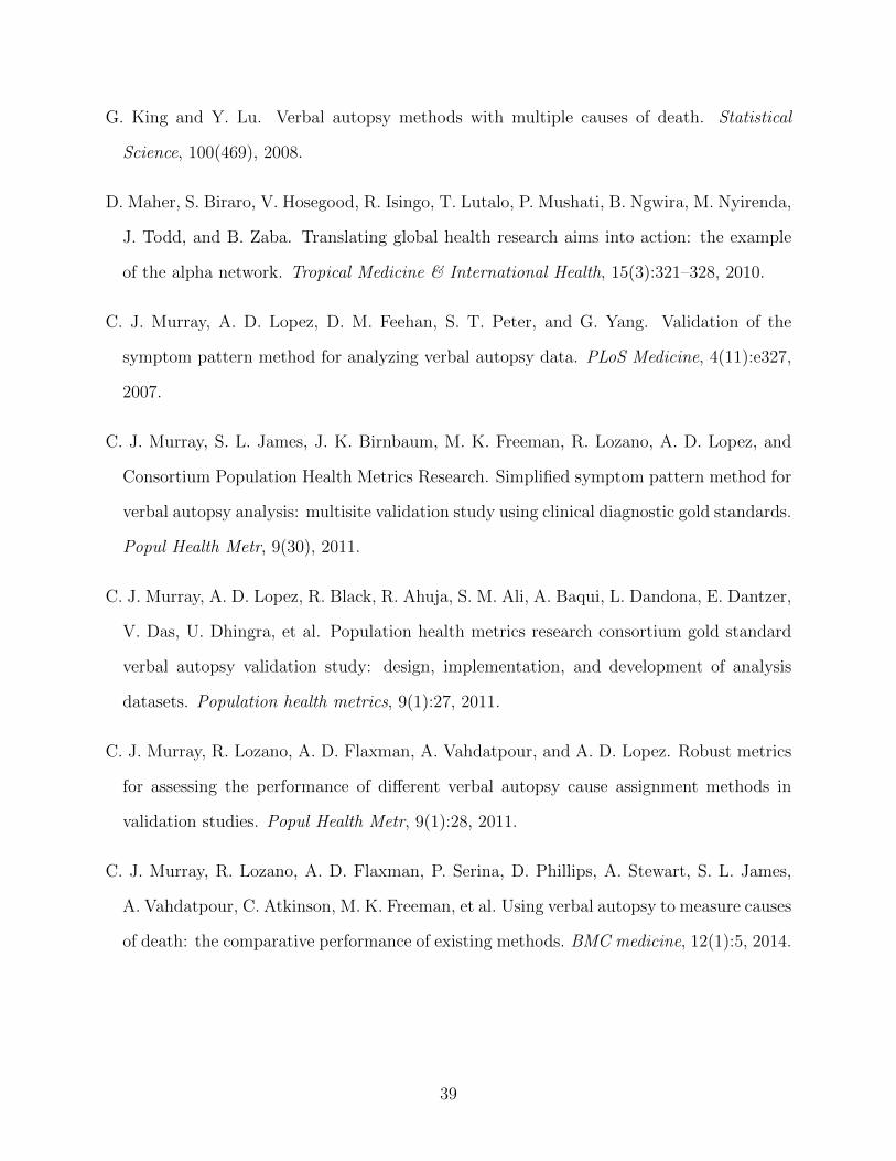
G. King and Y. Lu. Verbal autopsy methods with multiple causes of death. Statistical
Science, 100(469), 2008.
D. Maher, S. Biraro, V. Hosegood, R. Isingo, T. Lutalo, P. Mushati, B. Ngwira, M. Nyirenda,
J. Todd, and B. Zaba. Translating global health research aims into action: the example
of the alpha network. Tropical Medicine & International Health, 15(3):321–328, 2010.
C. J. Murray, A. D. Lopez, D. M. Feehan, S. T. Peter, and G. Yang. Validation of the
symptom pattern method for analyzing verbal autopsy data. PLoS Medicine, 4(11):e327,
2007.
C. J. Murray, S. L. James, J. K. Birnbaum, M. K. Freeman, R. Lozano, A. D. Lopez, and
Consortium Population Health Metrics Research. Simplified symptom pattern method for
verbal autopsy analysis: multisite validation study using clinical diagnostic gold standards.
Popul Health Metr, 9(30), 2011.
C. J. Murray, A. D. Lopez, R. Black, R. Ahuja, S. M. Ali, A. Baqui, L. Dandona, E. Dantzer,
V. Das, U. Dhingra, et al. Population health metrics research consortium gold standard
verbal autopsy validation study: design, implementation, and development of analysis
datasets. Population health metrics, 9(1):27, 2011.
C. J. Murray, R. Lozano, A. D. Flaxman, A. Vahdatpour, and A. D. Lopez. Robust metrics
for assessing the performance of different verbal autopsy cause assignment methods in
validation studies. Popul Health Metr, 9(1):28, 2011.
C. J. Murray, R. Lozano, A. D. Flaxman, P. Serina, D. Phillips, A. Stewart, S. L. James,
A. Vahdatpour, C. Atkinson, M. K. Freeman, et al. Using verbal autopsy to measure causes
of death: the comparative performance of existing methods. BMC medicine, 12(1):5, 2014.
39