Embed Size (px)
Citation preview

PRINCIPAL COMPONENT ANALYSISWITH MULTIRESOLUTION
By
VICTOR L. BRENNAN
A DISSERTATION PRESENTED TO THE GRADUATE SCHOOLOF THE UNIVERSITY OF FLORIDA IN PARTIAL FULFILLMENT
OF THE REQUIREMENTS FOR THE DEGREE OFDOCTOR OF PHILOSOPHY
UNIVERSITY OF FLORIDA
2001

ACKNOWLEDGMENTS
I am grateful for the support I have received from family, colleagues, and
faculty at UF. It is difficult to single out a few people to thank when many have
been supportive and encouraging.
I wish to thank my advisor, Dr. Jose Principe, not only for sharing his
technical expertise and insight, but especially for his patience and encouragement.
I want to thank Leonard and Carolina Brennan, who have been loving parents and
inspirational role models. I am most grateful to my wife, Karen, for her love and
for her support in every endeavor in our lives.
ii

TABLE OF CONTENTS
page
ACKNOWLEDGMENTS . . . . . . . . . . . . . . . . . . . . . . . . . . . . . ii
LIST OF TABLES . . . . . . . . . . . . . . . . . . . . . . . . . . . . . . . . . vi
LIST OF FIGURES . . . . . . . . . . . . . . . . . . . . . . . . . . . . . . . . vii
ABSTRACT . . . . . . . . . . . . . . . . . . . . . . . . . . . . . . . . . . . . x
CHAPTERS
1 INTRODUCTION . . . . . . . . . . . . . . . . . . . . . . . . . . . 1
1.1 Classification . . . . . . . . . . . . . . . . . . . . . . . . . . . 21.2 Principal Component Analysis (PCA) . . . . . . . . . . . . . 41.3 Multiresolution . . . . . . . . . . . . . . . . . . . . . . . . . 51.4 PCA-M . . . . . . . . . . . . . . . . . . . . . . . . . . . . . . 61.5 Image Classification Experiments . . . . . . . . . . . . . . . 61.6 MSTAR Experiment . . . . . . . . . . . . . . . . . . . . . . . 7
2 PCA . . . . . . . . . . . . . . . . . . . . . . . . . . . . . . . . . . . 9
2.1 The Eigenvalue Problem . . . . . . . . . . . . . . . . . . . . 92.2 An Example . . . . . . . . . . . . . . . . . . . . . . . . . . . 112.3 PCA . . . . . . . . . . . . . . . . . . . . . . . . . . . . . . . 152.4 Deflation Techniques . . . . . . . . . . . . . . . . . . . . . . 172.5 Generalized Hebbian Algorithm . . . . . . . . . . . . . . . . 192.6 Eigenfilters . . . . . . . . . . . . . . . . . . . . . . . . . . . . 22
2.6.1 Low-Pass Test Signal . . . . . . . . . . . . . . . . . . 232.6.2 High Pass Test Signal . . . . . . . . . . . . . . . . . . 252.6.3 Mixed Mode Test Signal . . . . . . . . . . . . . . . . . 26
2.7 Properties . . . . . . . . . . . . . . . . . . . . . . . . . . . . 27
3 MULTIRESOLUTION . . . . . . . . . . . . . . . . . . . . . . . . . 29
3.1 Two Notes Example . . . . . . . . . . . . . . . . . . . . . . . 303.2 Quadrature Filter and Iterated Filter Bank . . . . . . . . . . 323.3 Discrete Wavelets . . . . . . . . . . . . . . . . . . . . . . . . 343.4 Haar Wavelet . . . . . . . . . . . . . . . . . . . . . . . . . . 353.5 A Multiresolution Application: Compression . . . . . . . . . 35
iii

4 PCA-M . . . . . . . . . . . . . . . . . . . . . . . . . . . . . . . . . 38
4.1 Definition of PCA-M . . . . . . . . . . . . . . . . . . . . . . 384.1.1 Localization of PCA . . . . . . . . . . . . . . . . . . . 384.1.2 A Structure of Localized Outputs . . . . . . . . . . . 41
4.2 The Classification Problem . . . . . . . . . . . . . . . . . . . 434.3 Complete Representations . . . . . . . . . . . . . . . . . . . 44
4.3.1 Eigenfaces . . . . . . . . . . . . . . . . . . . . . . . . 454.3.2 Identity Map . . . . . . . . . . . . . . . . . . . . . . . 504.3.3 Iterated Filter Banks . . . . . . . . . . . . . . . . . . 524.3.4 Dual Implementation of PCA . . . . . . . . . . . . . . 56
4.4 Overcomplete Representations . . . . . . . . . . . . . . . . . 594.5 Local Feature Analysis . . . . . . . . . . . . . . . . . . . . . 60
4.5.1 Output Vector . . . . . . . . . . . . . . . . . . . . . . 614.5.2 Residual Correlation . . . . . . . . . . . . . . . . . . . 624.5.3 Kernel . . . . . . . . . . . . . . . . . . . . . . . . . . 634.5.4 LFA on ORL Faces . . . . . . . . . . . . . . . . . . . 634.5.5 Localization for LFA and PCA-M . . . . . . . . . . . 664.5.6 Feature Space for LFA, PCA, and PCA-M . . . . . . . 67
4.6 Summary . . . . . . . . . . . . . . . . . . . . . . . . . . . . . 67
5 FACE RECOGNITION EXPERIMENT . . . . . . . . . . . . . . . 69
5.1 ORL face Database . . . . . . . . . . . . . . . . . . . . . . . 705.2 Eigenfaces . . . . . . . . . . . . . . . . . . . . . . . . . . . . 71
5.2.1 Description of Experiment . . . . . . . . . . . . . . . 725.2.2 Results . . . . . . . . . . . . . . . . . . . . . . . . . . 73
5.3 Face Recognition using HMM’s . . . . . . . . . . . . . . . . . 735.3.1 Markov Models . . . . . . . . . . . . . . . . . . . . . . 745.3.2 Description of Experiment . . . . . . . . . . . . . . . 755.3.3 Results . . . . . . . . . . . . . . . . . . . . . . . . . . 76
5.4 Convolutional Neural Networks . . . . . . . . . . . . . . . . . 775.4.1 Self-Organizing Map . . . . . . . . . . . . . . . . . . . 775.4.2 Convolutional Network . . . . . . . . . . . . . . . . . 785.4.3 Description of Experiment . . . . . . . . . . . . . . . 795.4.4 Results . . . . . . . . . . . . . . . . . . . . . . . . . . 80
5.5 Face Classification with PCA-M . . . . . . . . . . . . . . . . 805.5.1 Classifier Architecture . . . . . . . . . . . . . . . . . . 815.5.2 Data Preparation . . . . . . . . . . . . . . . . . . . . 825.5.3 Fixed Resolution PCA Results . . . . . . . . . . . . . 825.5.4 Haar Multiresolution . . . . . . . . . . . . . . . . . . . 845.5.5 PCA-M . . . . . . . . . . . . . . . . . . . . . . . . . . 85
iv

6 MSTAR EXPERIMENT . . . . . . . . . . . . . . . . . . . . . . . . 88
6.1 SAR Image Database . . . . . . . . . . . . . . . . . . . . . . 896.2 Classification Experiment . . . . . . . . . . . . . . . . . . . . 906.3 Basis Arrays for PCA-M . . . . . . . . . . . . . . . . . . . . 93
6.3.1 Level 3 Components . . . . . . . . . . . . . . . . . . . 946.3.2 Level 2 Components . . . . . . . . . . . . . . . . . . . 946.3.3 Level 1 Components . . . . . . . . . . . . . . . . . . . 946.3.4 Decorrelation between Levels . . . . . . . . . . . . . . 95
6.4 A Component Classifier . . . . . . . . . . . . . . . . . . . . . 966.5 Classifications using Several Components . . . . . . . . . . . 986.6 A Simple Discriminator . . . . . . . . . . . . . . . . . . . . . 1026.7 False-Positive and False-Negative Errors . . . . . . . . . . . . 1046.8 Observations . . . . . . . . . . . . . . . . . . . . . . . . . . . 106
7 CONCLUSIONS AND FURTHER WORK . . . . . . . . . . . . . . 108
7.1 Conclusions . . . . . . . . . . . . . . . . . . . . . . . . . . . 1087.2 Future Work . . . . . . . . . . . . . . . . . . . . . . . . . . . 111
7.2.1 Segmentation of the Input . . . . . . . . . . . . . . . . 1117.2.2 Component Selection . . . . . . . . . . . . . . . . . . 1117.2.3 Conditioned Data and Non-Linear Classifier . . . . . . 112
APPENDIX
A ABBREVIATIONS . . . . . . . . . . . . . . . . . . . . . . . . . . . 113
B OLIVETTI RESEARCH LABORATORY FACE DATABASE . . . 115
C MSTAR IMAGES . . . . . . . . . . . . . . . . . . . . . . . . . . . . 116
REFERENCES . . . . . . . . . . . . . . . . . . . . . . . . . . . . . . . . . . . 120
BIOGRAPHICAL SKETCH . . . . . . . . . . . . . . . . . . . . . . . . . . . . 124
v
LIST OF TABLES
Table page
4.1 Normalized Eigenvalues . . . . . . . . . . . . . . . . . . . . . . . . . . 49
4.2 Energy Distribution of Exemplars . . . . . . . . . . . . . . . . . . . . 49
5.1 Error Rates of Several Algorithms . . . . . . . . . . . . . . . . . . . . 71
5.2 Face Classification CN Architecture . . . . . . . . . . . . . . . . . . . 80
5.3 Fixed Resolution PCA Error Rates over 10 Runs . . . . . . . . . . . . 82
5.4 Error Rates for PCA-M with Magnitude of FFT . . . . . . . . . . . . 86
5.5 Component Misclassifications (200 Test Images) . . . . . . . . . . . . 87
6.1 Input Data . . . . . . . . . . . . . . . . . . . . . . . . . . . . . . . . . 90
6.2 Classification using First Component . . . . . . . . . . . . . . . . . . . 97
6.3 Misclassifications with Individual PCA-M Components . . . . . . . . . 99
6.4 Error Rate (5/68 = 7.4%) using 3 Components . . . . . . . . . . . . . 100
6.5 Error Rate (2/68 = 3.0%) using 10 Components . . . . . . . . . . . . 100
6.6 Overall Unconditional Pcc with Template Matching . . . . . . . . . . . 102
6.7 Overall Unconditional Pcc with PCA-M . . . . . . . . . . . . . . . . . 102
6.8 Determining an Threshold for Detection . . . . . . . . . . . . . . . . . 103
6.9 Ten Components without Rejection . . . . . . . . . . . . . . . . . . . 104
6.10 Ten Components with Rejection . . . . . . . . . . . . . . . . . . . . . 104
6.11 Detector Threshold . . . . . . . . . . . . . . . . . . . . . . . . . . . . 105
6.12 Performance at 90% Pd . . . . . . . . . . . . . . . . . . . . . . . . . . 106
vi

LIST OF FIGURES
Figure page
1.1 Conceptual Steps in a Classifier . . . . . . . . . . . . . . . . . . . . . 3
1.2 PCA-M Classifier . . . . . . . . . . . . . . . . . . . . . . . . . . . . . 7
2.1 Sample Data . . . . . . . . . . . . . . . . . . . . . . . . . . . . . . . . 12
2.2 Original (left) and Scaled (right) Data . . . . . . . . . . . . . . . . . 15
2.3 GHA Linear Network . . . . . . . . . . . . . . . . . . . . . . . . . . . 20
2.4 Low Pass Test Data . . . . . . . . . . . . . . . . . . . . . . . . . . . . 23
2.5 Low Pass Data PCA . . . . . . . . . . . . . . . . . . . . . . . . . . . 25
2.6 High Pass Data PCA . . . . . . . . . . . . . . . . . . . . . . . . . . . 26
2.7 Test High and Low Frequency Data . . . . . . . . . . . . . . . . . . . 27
3.1 Two Notes . . . . . . . . . . . . . . . . . . . . . . . . . . . . . . . . . 31
3.2 Quadrature Filter . . . . . . . . . . . . . . . . . . . . . . . . . . . . . 33
3.3 Discrete Wavelet Transform with 2 Levels . . . . . . . . . . . . . . . . 34
3.4 Equivalent 2m Filter Bank DWT Implementation . . . . . . . . . . . 35
3.5 Three Levels of Decomposition on the Approximation . . . . . . . . . 36
4.1 PCA-M for Classification . . . . . . . . . . . . . . . . . . . . . . . . . 40
4.2 PCA and PCA-M in Feature Space . . . . . . . . . . . . . . . . . . . 44
4.3 Raw Images from ORL Database . . . . . . . . . . . . . . . . . . . . 46
4.4 Residual Images for GHA Input . . . . . . . . . . . . . . . . . . . . . 46
4.5 All-to-one and One-to-one Networks . . . . . . . . . . . . . . . . . . . 47
4.6 Eigenfaces from GHA Weights . . . . . . . . . . . . . . . . . . . . . . 48
4.7 Three Level Dyadic Banks . . . . . . . . . . . . . . . . . . . . . . . . 52
4.8 First Four Eigenimages . . . . . . . . . . . . . . . . . . . . . . . . . . 54
vii

4.9 Three Level Decomposition of a Face . . . . . . . . . . . . . . . . . . 55
4.10 Output of Quadratic Filter Bank . . . . . . . . . . . . . . . . . . . . 55
4.11 Localization of a Global Output . . . . . . . . . . . . . . . . . . . . . 58
4.12 Local Feature Analysis . . . . . . . . . . . . . . . . . . . . . . . . . . 60
4.13 PCA Reconstruction MSE . . . . . . . . . . . . . . . . . . . . . . . . 64
4.14 PCA Reconstructions . . . . . . . . . . . . . . . . . . . . . . . . . . . 64
4.15 LFA Outputs (Compare to PCA Reconstruction) . . . . . . . . . . . 65
4.16 LFA Kernel and Residual Correlation (Look for Localization) . . . . . 66
5.1 Varying Conditions in ORL Pictures . . . . . . . . . . . . . . . . . . 71
5.2 Parsing an Image into a Sequence of Observations . . . . . . . . . . . 74
5.3 Markov Model . . . . . . . . . . . . . . . . . . . . . . . . . . . . . . . 75
5.4 Top-down Constrained State Transitions . . . . . . . . . . . . . . . . 75
5.5 SOM-CN Face Classifier . . . . . . . . . . . . . . . . . . . . . . . . . 77
5.6 Initial Classifier Structure . . . . . . . . . . . . . . . . . . . . . . . . 81
5.7 Training and Test Data at Different Scales . . . . . . . . . . . . . . . 83
5.8 PCA-M Decomposition of One Picture . . . . . . . . . . . . . . . . . 84
5.9 Selected Resolutions . . . . . . . . . . . . . . . . . . . . . . . . . . . 85
5.10 Final Classifier Structure . . . . . . . . . . . . . . . . . . . . . . . . . 86
6.1 Aspect and Depression Angles . . . . . . . . . . . . . . . . . . . . . . 89
6.2 Experiment Overview . . . . . . . . . . . . . . . . . . . . . . . . . . . 91
6.3 Three Levels of Decomposition on the Approximation . . . . . . . . . 93
6.4 PCA-M Decomposition of a BMP2 Input . . . . . . . . . . . . . . . . 95
6.5 The Templates for Three Classes for PCA-M Component 1 . . . . . . 96
6.6 First Component of SAR Images Projected to 3-Space . . . . . . . . . 98
6.7 Class Templates for other PCA-M Components . . . . . . . . . . . . 99
6.8 Clustering in 3-Space using All PCA-M Components . . . . . . . . . 101
6.9 Probability of Detection versus False Alarm Rate . . . . . . . . . . . 106
viii

B.1 Olivetti Research Laboratory Face Database . . . . . . . . . . . . . . 115
C.1 BMP2 Training and Test Data . . . . . . . . . . . . . . . . . . . . . . 116
C.2 T72 Training and Test Data . . . . . . . . . . . . . . . . . . . . . . . 117
C.3 BTR70 Training and Test Data . . . . . . . . . . . . . . . . . . . . . 118
C.4 Confuser Data . . . . . . . . . . . . . . . . . . . . . . . . . . . . . . . 119
ix

Abstract of Dissertation Presented to the Graduate Schoolof the University of Florida in Partial Fulfillment of theRequirements for the Degree of Doctor of Philosophy
PRINCIPAL COMPONENT ANALYSISWITH MULTIRESOLUTION
By
Victor L. Brennan
May 2001
Chair: Jose PrincipeMajor Department: Electrical and Computer Engineering
Eigenvalue decomposition and multiresolution are widely used techniques
for signal representation. Both techniques divide a signal into an ordered set of
components. The first component can be considered an approximation of the input
signal; subsequent components improve the approximation. Principal component
analysis selects components at the source resolution that are optimal for minimiz-
ing mean square error in reconstructing the original input. For classification, where
discriminability among classes puts an added constraint on representations, PCA
is no longer optimal. Features utilizing multiresolution have been demonstrated to
preserve discriminability better than a single scale representation. Multiresolution
chooses components to provide good representations of the input signal at several
resolutions. The full set of components provides an exact reconstruction of the
original signal.
x
Principal component analysis with multiresolution combines the best proper-
ties of each technique:
1. PCA provides an adaptive basis for multiresolution.
2. Multiresolution provides localization to PCA.
The first PCA-M component is a low-resolution approximation of the signal.
Additional PCA-M components improve the signal approximation in a manner
that optimizes the reconstruction of the original signal at full resolution. PCA-M
can provide a complete or overcomplete basis to represent the original signal,
and as such has advantages for classification because some of the multiresolution
projections preserve discriminability better than full resolution representations.
PCA-M can be conceptualized as PCA with localization, or as multiresolution
with an adaptive basis. PCA-M retains many of the advantages, mathematical
characteristics, algorithms and networks of PCA. PCA-M is tested using two
approaches. The first approach is consistent with a widely-known eigenface
decomposition. The second approach assumes ergodicity. PCA-M is applied to two
image classification applications: face classification and synthetic aperture radar
(SAR) detection. For face classification, PCA-M had an average error of under
2.5%, which compares favorably with other approaches. For synthetic aperture
radar (SAR), direct comparisons were not available, but PCA-M performed better
than the matched filter approach.
xi

CHAPTER 1INTRODUCTION
Principal component analysis with multiresolution (PCA-M) combines and
enhances two well-established signal processing techniques for signal representa-
tion. This dissertation presents the motivation, the mathematical basis, and an
efficient implementation for combining principal component analysis (PCA) with
multiresolution.
This dissertation also presents the results of using PCA-M as a front-end
for two applications: face classification, and target discrimination of synthetic
aperture radar (SAR) images. More detailed discussions of PCA, multiresolution
(differential pyramids), and PCA-M are presented in subsequent chapters. This
introduction is intended as an overview to the presentation of PCA-M.
PCA-M was originally developed as an on-line signal representation technique.
The intent was to perform real-time segmentation of (time) signals based on
variations in local principal components. Tests with simple artificially generated
signals were promising, and good results have been reported in applying PCA-M
to biological signals (Alonso-Betzanos et al., 1999). The decision to concentrate
on images was made when several researchers (Giles et al., 1997; Samaria, 1994;
Turk and Pentland, 1991a) applied various techniques against a common database
generated by the Olivetti Research Lab (ORL). Each of the researchers also cited
an approach which decomposed a set of facial images into component eigenfaces.
It became possible to compare the performance of PCA-M to the results of other
researchers using fixed resolution PCA technique and more computationally
1
2
intensive non-PCA image classification techniques. We will start by providing a
brief overview of the fundamental concepts required to understand PCA-M.
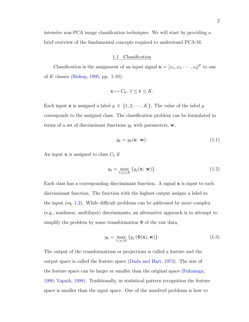
1.1 Classification
Classification is the assignment of an input signal x = [x1, x2, · · · , xd]T to one
of K classes (Bishop, 1995, pp. 1-10).
x 7→ Ck, 1 ≤ k ≤ K.
Each input x is assigned a label y ∈ {1, 2, · · · , K}. The value of the label y
corresponds to the assigned class. The classification problem can be formulated in
terms of a set of discriminant functions yk with parameters, w,
yk = yk(x; w). (1.1)
An input x is assigned to class Ck if
yk = max1≤j≤K
{yj(x; w)}. (1.2)
Each class has a corresponding discriminant function. A signal x is input to each
discriminant function. The function with the highest output assigns a label to
the input (eq. 1.2). While difficult problems can be addressed by more complex
(e.g., nonlinear, multilayer) discriminants, an alternative approach is to attempt to
simplify the problem by some transformation Φ of the raw data,
yk = max1≤j≤K
{yj (Φ(x),w)}. (1.3)
The output of the transformations or projections is called a feature and the
output space is called the feature space (Duda and Hart, 1973). The size of
the feature space can be larger or smaller than the original space (Fukunaga,
1990; Vapnik, 1998). Traditionally, in statistical pattern recognition the feature
space is smaller than the input space. One of the unsolved problems is how to
3
determine the feature space and its size to improve classification accuracy. A
feature is a projection that preserves discriminability. A fortuitous choice for
the transformation extracts features that differ between classes but are similar
within a class. Undesirable features differ within-class or are similar between-class.
Heuristics have been the most utilized method of selecting good features.
The problem is the following. Optimal classifications in high dimensional
spaces require prohibitive amounts of data to be trained accurately (Fukunaga,
1990; Duda and Hart, 1973). Hence the reduction of the input space dimensionality
improves accuracy of the estimated classifier parameters and improves classifier
performance. On the other hand, projections to a feature subspace may decrease
discriminability, so there is a trade-off that is difficult to formulate and solve (Fuku-
naga, 1990).
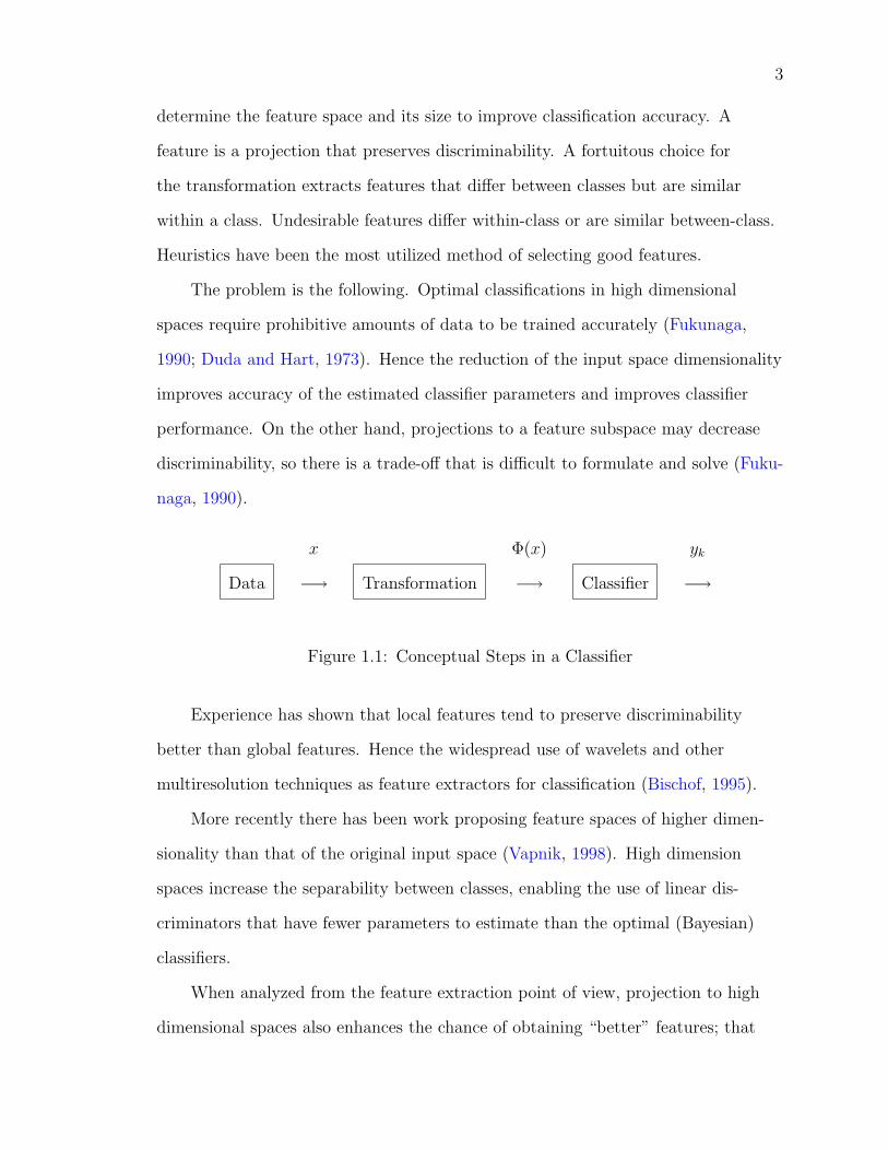
Data
x
−→ Transformation
Φ(x)
−→ Classifier
yk
−→
Figure 1.1: Conceptual Steps in a Classifier
Experience has shown that local features tend to preserve discriminability
better than global features. Hence the widespread use of wavelets and other
multiresolution techniques as feature extractors for classification (Bischof, 1995).
More recently there has been work proposing feature spaces of higher dimen-
sionality than that of the original input space (Vapnik, 1998). High dimension
spaces increase the separability between classes, enabling the use of linear dis-
criminators that have fewer parameters to estimate than the optimal (Bayesian)
classifiers.
When analyzed from the feature extraction point of view, projection to high
dimensional spaces also enhances the chance of obtaining “better” features; that

4
is, where the projections of different classes concentrated more along certain
directions. These are called overcomplete representations and they have been
studied in the wavelet literature (Vetterli and Kovacevic, 1995; Strang and Nguyen,
1996). The big issue is still how to choose the overcomplete dictionary and how to
select the best features.
1.2 Principal Component Analysis (PCA)
Principal component analysis (PCA) is based on eigenvalue decomposi-
tion (Hotelling, 1933). Eigenvalue decomposition has been applied to problems
across many disciplines. There is a rich mathematical background and a variety of
implementations (Oja, 1982). Given a set of data, a scatter matrix S is calculated
to estimate the autocorrelation matrix of the data.
S =1N
N∑
n=1
xnxTn . (1.4)
The eigenvector and corresponding eigenvalue pairs (wk, λk) of S are found by
solving
Sw = λw. (1.5)
Both the data x and the scatter matrix S can be expanded in terms of the eigen-
vectors,
S =∑
k wkwTk λk,
x =∑
k wkwTk x =
∑
k wkαk.(1.6)
Analytic and deflation-based iterative approaches are available to solve the eigen-
value problem that automatically order the eigenvectors such that
λ1 > λ2 > . . . > λN .

5
PCA components are uncorrelated and maximal in l2 energy. PCA is one possible
transformation for equation 1.3. It has been shown that PCA is optimal for signal
representation, but it is sub-optimal for feature extraction (Fukunaga, 1990).
Chapter 2 has an expanded discussion of PCA. Although other sets of basis
functions are available that are similar to the PCA basis, only PCA can select a
reduced set of components that are optimal for reconstruction MSE.
1.3 Multiresolution
Multiresolution has been broadly defined as the simultaneous presentation
of a signal at several resolutions. An intuitive argument for using multiresolution
is available from common experience. Consider watching someone approach from
a distance. As the person comes closer, more details are resolvable to allow an
observer to make successively refined categorizations. A possible sequence is to first
identify a moving object, then a person, the gender of the person, the identity of
the person, and finally the facial expressions of the person.
Another familiar application of multiresolution is transferring images across
low bandwidth channels (internet). People tend to leave a web page if the page
takes too long to load. For commercial web sites this translates into a loss of
potential customers. On the other hand, many sites feel that customers will not
return to a site that does not have a lot of graphics. Some image intensive web
pages (e.g., zoo, museum, or auction sites) usually present small images (initially
transfer small files). A larger, more detailed version of the image is loaded only
if the viewer clicks on the small image. While it is possible to completely reload
the larger image, it is more efficient to use information available on the (already
loaded) small version and just add the details needed to produce the larger picture.
For classification, it is hoped that within-class differences are high-resolution
features, and that sufficient desirable features are resolvable at coarse resolution.
By using a coarser representation (lower-resolution), it is hoped that undesirable

6
features are sharply attenuated with minor impact on the desirable features.
Multiresolution is discussed in chapter 3.
1.4 PCA-M
Both PCA and multiresolution have been successfully applied to similar
problems. It seems reasonable that an application that has benefited from each
individual approach should further benefit from a combined approach. PCA-M is
simply multiresolution with an adaptive basis (PCA).
I show that a linear network for online, adaptive, multiresolution feature
extraction is easily adapted from the networks used for standard PCA. principal
component analysis with multiresolution (PCA-M) is implemented with a partially
connected, single-layer linear network. The same network can be used for both
training and normal operation. The training algorithm is a modification of the
generalized hebbian algorithm (GHA) (Sanger, 1989). I treat PCA-M in chapter 4.
1.5 Image Classification Experiments
Olivetti Research Lab (ORL) has a public face database that serves as a
benchmark for comparing different face classification algorithms. Both mul-
tiresolution and PCA (Turk and Pentland, 1991a) had been successfully applied
against the database. The PCA-M components were used with an almost linear
network. The network is linear except for selecting the maximum discriminant
(MAXNET) (Kung, 1993, p. 48)).

7
Figure 1.2: PCA-M Classifier
The ORL database was used to compare PCA-M to several standard fixed
resolution transforms (discrete Fourier transform, discrete cosine transform, PCA),
and to multiresolution using a Haar basis. PCA-M outperformed PCA at all tested
resolutions. PCA-M outperformed the Haar basis if a reduced set of components
were used. Results were comparable if the full set of multiresolution components
were used.
In chapter 5, PCA-M results are compared to classifiers using a fixed res-
olution PCA (Turk and Pentland, 1991a, Eigenfaces), a hidden Markov model
(HMM) (Samaria, 1994) and a convolutional neural network (Giles et al., 1997).
PCA-M had the lowest error rate.
1.6 MSTAR Experiment
The 9/95 MSTAR Public Release Data (Veda Inc., www.mbvlab.wpafb.mil).
contains synthetic aperture radar (SAR) images of vehicles at various poses (aspect
and depression angles). The estimated aspect angle (Xu et al., 1998) of each
vehicle was used to assign each vehicle to one of the twelve non-overlapping 30◦
sectors. Within each sector, multiresolution templates were derived for each class.
Chapter 6 shows that PCA-M worked very well in some sectors, but poorly in other
sectors. The overall error rate ( 10%) was comparable to other template matching

8
procedures (Velten et al., 1998), but poorer than information theoretic and vector
support methods.
We conclude the dissertation with some comments and future directions for
further research.

CHAPTER 2PRINCIPAL COMPONENT ANALYSIS
Principal component analysis (PCA) is a technique for representing an image
(or a signal) using basis functions that are derived from eigenvalue decomposi-
tion of the data autocorrelation matrix. This chapter is an introduction to the
eigenvalue problem. A thorough presentation is not possible, but this chapter
should contain the information on principal component analysis that is required by
subsequent discussion of PCA-M.
2.1 The Eigenvalue Problem
Consider a square matrix A of full rank N . A vector w is said to be an
eigenvector of A with a corresponding (scalar) eigenvalue λ if
Aw = λw. (2.1)
The eigenvalue problem (equation 2.1) can be solved analytically by subtracting
λw from both sides,
(A− Iλ)w = 0. (2.2)
Taking the determinant of both sides yields an N th order polynomial in λ called the
characteristic polynomial of A,
det(|A− Iλ|) = 0. (2.3)
The N roots are the eigenvalues, and each eigenvalue λk has a corresponding eigen-
vector wk. Each solution to the eigenvector problem is a paired eigenvalue and
corresponding eigenvector (λk,wk). From equation 2.1, it should be clear that if w
9

10
is an eigenvector and κ is an arbitrary scalar, then κw is also an eigenvector with
the same eigenvalue. Given a non-repeating eigenvector λ, the corresponding eigen-
vector is unique except for scale factor κ. Without loss of generality, eigenvectors
are usually scaled such that
|w| =√
wTw = 1.
If the eigenvalues λk are unique (non-repeated), then a unique eigenvector exists for
each eigenvalue. The (normalized) eigenvectors wk are orthonormal.
wTj wk = δjk. (2.4)
Define the modal matrix W as the matrix whose columns are the normalized
eigenvectors of A,
W = [w1 w2 . . . wN ] (2.5)
In general, there are N ! permutations of eigenvectors. Without loss of generality,
order the eigenvectors such that the eigenvalues are non-increasing,
λ1 ≥ λ2 ≥ . . . ≥ λN .
Define the diagonal matrix Λ as the matrix with a main diagonal consisting of the
(ordered) eigenvalues of A.
Λ =
λ1 0 · · · 0
0 λ2 . . . 0...
... . . . ...
0 0 · · · λN .
The eigenvalue problem can be restated in matrix notation,
A = WΛW T . (2.6)

11
If equation 2.6 is satisfied, the matrix A is said to be diagonalizable. For this study,
the matrices of interest are real Toeplitz matrices that are always diagonalizable.
The orthonormality condition of equation 2.4 can also be restated,
WW T = W T W = I. (2.7)
A matrix satisfying equation 2.7 is said to be unitary. The modal matrix W is
unitary and is said to diagonalize the matrix A.
2.2 An Example
The properties of PCA will later be discussed more rigorously, but a quick
example should provide an intuitive grasp of some of the properties of PCA.
Consider L = 20 vectors of dimension N = 3 arranged into the data matrix X,
X = [x1 x2 . . . x20]
The autocorrelation of the data is estimated by the scatter matrix,
Sxx = E{xx′} =1L
XX ′ =
0.1296 0.1372 0.1296
0.1372 0.1613 0.1372
0.1296 0.1372 0.1296
.
Eigenvalue decomposition yields
W =
0.5578 −0.4346 −0.7071
0.6146 0.7888 0.0000
0.5578 −0.4346 0.7071
, Λ =
0.4104 0 0
0 0.0102 0
0 0 0
.
Each input vector can be interpreted as a set of coordinates. The standard
basis functions for the input space are normalized vectors in each of the input

12
coordinates,
e1 =
1
0
0
, e2 =
0
1
0
, e3 =
0
0
1
.
Figure 2.1 (left) plots the data in the input space. The input was constructed to
lie near the diagonal of the input space. The first element of each input vector
was randomly selected in the interval (−1, +1). The second element was the
first element plus Gaussian noise. The third element was set equal to the first
component. By construction, all three elements are equal except for the additive
Gaussian noise in the second element. The dimension of the signal (part of x
excluding the noise) is one. The noise adds a second dimension. Although x is
nominally three-dimensional, the data set can be embedded in a two-dimensional
space.
Figure 2.1: Sample Data
Figure 2.1 (middle) shows the eigenvectors in the input space. Note that the
first eigenvector is the line that best fits the data in a mean square error sense.
Figure 2.1 (right) shows that the eigenvectors can be used as basis functions for

13
the data. The input coordinates x are rotated to the eigenspace coordinates y by
multiplication with the modal matrix W ,
y = W Tx or Y = W T X.
The input vectors were drawn from a zero mean distribution, but the sample mean
was
x = E{x} = [0.1476, 0.1649, 0.1476]T .
If the data is zero-mean, then the scatter matrix is also an estimate of the auto-
covariance. The shift, z = x − x , would produce data with a (sample) mean
of zero. It is obvious in this example that the sample mean is a poor estimate
of the true mean. The true mean of the output is zero, but the sample mean is
y = [0.2660, 0.0018, 0.0000],
y = E{y} = W T x.
It is perhaps too obvious to mention that small sample sizes lead to poor char-
acterization (e.g., statistical parameters) of a distribution. However, many real
applications have a limited amount of data available. Insufficient data will degrade
the performance of any algorithm. The scatter matrix of the rotated vectors is
Syy = Λ. Since Λ is diagonal, the components of y are uncorrelated.
Syy =1L
Y Y T =1L
W T XXT W = W T SxxW = Λ.
The trace of the scatter matrices is invariant under rotation,
Sxx = Syy = 0.4206
The trace is a measure of the total variation of the data. A linear transformation
does not affect total autocorrelation. However, a linear transformation can change

14
the variance of individual components and the cross-correlation between compo-
nents. To see the contribution of each component of the input and output to the
total variance, divide both scatter matrices by the trace,
S ′xx =
0.3082 0.3262 0.3082
0.3262 0.3836 0.3262
0.3082 0.3262 0.3082
, S ′yy =
0.9758 0 0
0 0.0242 0
0 0 0
.
The trace of each scatter matrix in equation 2.2 is one, and the elements along the
main diagonal can be interpreted as percentages of total variation. By construction
the variation in the input data is distributed almost equally among all three
components. The normalized output scatter matrix (equation 2.2) shows that the
first component captures 97.6% of the variation of the data. The zero eigenvalue
in the third column of Λ indicates that the underlying dimension of the data is two.
The input data can be reconstructed from the output data,
x = Wy or X = WY.
The input data can be perfectly reconstructed from y even if the third component
is discarded (33% lossless compression). The input data can be reconstructed with
2.5% mean square error from just the first component of y (67% compression).
The transform did not completely separate the data from the noise. However,
the input reconstructed from just the first output component has an enhanced
signal-to-noise ratio (SNR).
The rotation from the input space X to the eigenspace Y is only one possible
rotation. Although it is more obvious to directly examine other rotations of the
3-dimensional input space, it is simpler to examine rotations of the 2-dimensional
eigenspace. Consider a set of coordinates z derived from rotating the (non-zero)

15
coordinates in eigenspace through an arbitrary angle α,
z =
z1
z2
=
cos(α) sin(α)
− sin(α) cos(α)
y1
y2
The variance of {z1} is
σ2z1z1
= cos2(α)σ2y1y1
+ sin2(α)σ2y2y2
.
Figure 2.2: Original (left) and Scaled (right) Data
Figure 2.2 (left) shows the standard deviations of the two non-zero components
of the output. The ellipse in figure 2.2 (left) shows the standard deviations of the
data projected along arbitrary unit vectors. Among all possible sets of projections,
the variance of an individual component is maximized and minimized when the
input is projected against the two eigenvectors w1 and w2, respectively. If
the second component is scaled so that the variances of the two components are
equal (Figure 2.2, right), it is not possible to change the component variances by
rotation.
2.3 Principal Component Analysis
The Karhunen-Loeve Transform (KLT) uses eigenvalue analysis to decompose
a continuous random process, x(t), instead of the random variable discussed in the

16
preceding sections of this chapter. The discrete equivalent developed by Hotelling
is called Principal component analysis (PCA), but is also often referred to as
Karhunen-Loeve Transformation. A nice discussion is found in Jain (1989, pp.
163-175).
Let x be a discrete zero-mean, wide-sense stationary process. Let xN(n)
denote a block of length N ,
xN(n) = [x(n), x(n− 1), · · · , x(n−N + 1)]T .
The (N ×N) autocorrelation matrix RXX is positive-definite and Toeplitz (doubly
symmetric and constant along the diagonals) (Kailath, 1980). The eigenvalue
decomposition of RXX is
RXX = E{xN(n)xN(n)T} = W Λ W−1 = W Λ W T
Not all matrices can be diagonalized, but symmetry is a sufficient condition. Since
RXX is symmetric, it has N orthogonal eigenvectors even if the eigenvalues are
not distinct. PCA is an expansion of xN(n) using the eigenvectors of RXX . Any
N-length block of x(n) can be represented by
xN(n) =N
∑
k=1
x(n− k + 1)ek =N
∑
k=1
yk(n)wk.
The PCA expansion can be more compactly expressed by
xN(n) = WyN(n), with inverse, yN(n) = W TxN(n), (2.8)
where
yN(n) = [y1(n), y2(n), · · · , yN(n)]T .
Equation 2.8 can also be interpreted as linear mappings from an N -dimensional
space spanned by the standard basis vectors, ek, to an N -dimensional space

17
spanned by the eigenvectors, wk. The autocorrelation matrix of yN(n) is
RY Y = E{yN(n)yN(n)T} = E{W TxN(n)xN(n)T W}
= W T E{xN(n)xN(n)T}W
= W T RXXW = Λ
Λ represents the correlation matrix between the components yk. The components
are uncorrelated and the variance of each component is simply λk. Interpreting
variance as signal energy, trace-invariance under similarity transformations equates
to conservation of energy. The original signal can be perfectly reconstructed by the
inverse transformation,
x(n)
x(n− 1)...
x(n−N + 1)
= W
y1(n)
y2(n)...
yN(n)
(2.9)
Decorrelation is desirable for analysis since redundant information between
components is minimized. Reconstruction is often performed with only the first
M < N components for two main reasons,
1. Compression - Using only the first M components achieves a M/N compres-
sion ratio with minimum l2 reconstruction error.
2. Noise Reduction - For signals with additive noise, Λ is interpreted as a signal
to noise ratio (SNR). Reconstruction of x(n) using the high SNR components
retains the signal components and excludes the noisy low energy components.
2.4 Deflation Techniques
All the eigenvalues of a matrix of rank N can be found analytically by solving
a polynomial of order N ,
det(A− Iλ) = 0.

18
If only the first few eigenvectors are of interest, then one can either use an analyti-
cal approach such as Singular Value Decomposition (SVD) (Haykin, 1996), or find
an approximation by using a deflation technique. Since the one of the eigenvectors
maximizes variance, a vector is found by choosing an arbitrary vector and itera-
tively modifying the vector to increase the variance. Once found, the component
corresponding to the eigenvector is removed and the input is said to be deflated.
The next eigenvector is found by repeating the process on the deflated data. From
the basic eigenvalue statement (equation 2.1),
λk = wTk Awk (2.10)
Consider an arbitrary vector v and an associated scalar κ,
κ = vT Av (2.11)
The eigenvector corresponding to the largest eigenvalue maximizes
λ1 = max(κ) = max∀v
{
vT Av}
(2.12)
Equation 2.11 associates a scalar with each of the vectors in the span of A. The
vector associated with the maximal scalar is an eigenvector of A. More specifically,
1. Set A1 = A.
2. Use a gradient based iteration (or power method) on w to maximize λ.
3. Set w1 = wopt and λ1 = λ(wopt).
4. Remove the projection of w1 from A1.
A2 = A1 −w1λ1wT1
5. In the subspace spanned by A2 the optimal solution to equation 2.12 is
now {λ2,w2}. Repeat procedure until the desired number of solutions
(eigenvectors) is obtained.
19
2.5 Generalized Hebbian Algorithm
Eigendecompositions can be analytically computed by many algorithms (Golub
and Loan, 1989). But here we seek sample-by-sample estimators of PCA conducive
to on-line implementation in personal computers. There is rich literature on linear
networks to evaluate PCA using gradient descent learning rules (Oja, 1982; Haykin,
1994). Being adaptive, the networks take time to converge and exhibit rattling;
that is, network values fluctuate around the “true” values. Hence, these networks
should not be taken as substitutes for the analytic methods when the goal is to
compute eigenvectors and eigenvalues. However, in signal processing applications
where we have to deal with nonstationary signals and we are interested in feature
vectors for real-time assessment, the “noisy” PCA is very often adequate and saves
enormous computation. In fact, the algorithms about to be described are of O(N)
(size of the space), instead of O(N2).
Haykin (1994, pp. 391) states that PCA neural network algorithms can be
grouped into two classes:
1. reestimation algorithms - only feedforward connections,
2. decorrelating algorithms - both feedforward and feedback connections.
Reestimation algorithms use deflation. The generalized hebbian algorithm (GHA)
is a reestimation algorithm that uses a single (computational) layer linear network
to perform PCA on a process xN(n). A nice presentation of GHA can be found in
Haykin (1994, pp. 365-394).

20
Figure 2.3: GHA Linear Network
Let W denote the (M × N) matrix of network weights and let wk denote
a column of W . Figure 2.3 shows the network that extracts the first M ≤ N
principal components of the random vector xN(n). The equations for figure 2.3 are
yM(n) = W TxN(n) =
wT1
wT2
...
wTM
xN(n), M ≤ N.
To adapt the weights, GHA performs three operations,
1. adaptation of each column wi to maximize variance (energy),
2. adaptation between columns wi to remove the projection from previous
components,
3. self-normalizing to keep weights at unit norm.

21
The equations for adapting the weights are
yj(n) =p−1∑
i=0
wji(n)xi(n), calculate output (2.13)
∆wji(n) = ηyj(n)
[
xi(n)−j
∑
k=0
wki(n)yk(n)
]
, update weights (2.14)
The update (equation 2.14) has two terms,
η(yj(n)xi(n)− yj(n)wji(n)yj(n)), maximize variance and normalize (2.15)
−ηyj(n)j−1∑
k=0
wki(n)yk(n), remove projections (2.16)
Equation 2.15 has two terms. The first term is the classic Hebbian formulation
and has been called the activity product rule (Haykin, 1994, p. 51). The problem
with the classic formulation is that the magnitude of the weights increases. Still,
the classic Hebbian algorithm is elegant in its simplicity and power. The second
term of equation 2.15 is a self correcting adaptation (Sanger, 1989). Equation 2.15
by itself reestimates and normalizes the weights for variance maximization. Equa-
tion 2.16 subtracts the projections of previous (higher energy) components. This
term is introduced to keep the weights to different output nodes from converging
to the same eigenvector. Equation 2.16 also shows that convergence of a principal
component is dependent on the convergence of higher energy components. While
there is no inherent ordering to the eigenvectors, the implementation effectively
creates a sequence of dependencies in the convergence of eigenvectors.
The procedure is adaptive and thus suitable for locally stationary data. Even
if the process is not stationary, the mapping W TNxN will give perfect reconstruction
(WNxN is invertible). PCA is optimal for minimum l2 reconstruction using fixed
length filters on a stationary signal. For optimal l2 compression and reconstruction,
the first M (out of N) components of yN(n) are used.

22
Using M < N components yields a compression of (N −M)/N . Further com-
pression is usually obtained by using fewer bits to encode lower energy components.
−→yc (k) = [y0(k), y1(k), · · · , yM−1(k)]T = W TN×MxN(n). (2.17)
and the reconstruction (denoted by subscript c)of the original signal is
−→xc (k) =[
(WN×MW TN×M)−1WN×M
]−→yc (k). (2.18)
2.6 Eigenfilters
The direct interpretation of equation 2.8 is that each of the yk(n) is a projec-
tion of xN(n) on an eigenvectors wk. Each projection is found by taking the inner
product,
yk(n) = 〈wk,xN(n)〉 = wTk xN(n) (2.19)
The underlying time structure of xN(n) allows a filter interpretation of PCA,
xN(n) = [x(n), x(n− 1), · · · , x(n−N + 1)]T .
Rewriting equation 2.19,
yk(n) = wTk xN(n) =
N−1∑
α=0
wk(α) x(n− α). (2.20)
Equation 2.20 is a convolution sum of x with a filter impulse response wk(n). FIR
filters whose coefficients (impulse response) are derived from eigenvalue analysis are
called eigenfilters (Vetterli and Kovacevic, 1995). The collection of filters, {wi}i can
be interpreted as an analysis bank. If the principal components,
y(n) = [y1(n), y2(n), · · · , yN(n)]T .
are then processed to reconstruct the original input xN(n), the reconstruction
filters form the synthesis bank. Eigenfilters have several key properties:

23
1. Both the analysis and synthesis banks of a linear network use finite impulse
response (FIR) filters,
2. Since the autocorrelation filter is Toeplitz, the eigenvectors are all either
symmetric or antisymmetric,
3. Since the modal matrix is unitary, the synthesis filters can be implemented
easily (transpose of the analysis bank),
4. Since the components are uncorrelated, the reconstruction from each compo-
nent is independent of other components.
The remainder of this section illustrates the decomposition of simple test signals.
2.6.1 Low-Pass Test Signal
Figure 2.4: Low Pass Test Data
A test signal (Figure 2.4) was generated using a 5th-order moving average
(MA) filter driven by white Gaussian noise.
x (n) =12
5∑
k=0
2−ku (n− k) ⇔ X(z) =12
5∑
k=0
(2z)−k U (z)

24
The transfer function is
H (z) =X (z)U (z)
=12
[
1 +(
12z
)
+(
12z
)2
+(
12z
)3
+(
12z
)4
+(
12z
)5]
The 5 zeros are evenly spaced,
z−1 =12
exp(
jkπ3
)
, k ∈ [1, 2, 3, 4, 5]
The first six autocorrelation coefficients are
RXX(k, 1) =[
0.3333 0.1665 0.0830 0.0410 0.0195 0.0078
]T
Consider the autocorrelation matrix formed by the first six autocorrelation coeffi-
cients. The eigenvalues are
λk =[
0.7952 0.4811 0.2811 0.1859 0.1388 0.1174
]
The corresponding eigenvectors (columns) are
W =
0.3034 −0.4940 −0.5350 −0.4721 −0.3489 0.1819
0.4195 −0.4687 −0.1244 0.3313 0.5554 −0.4130
0.4816 −0.1905 0.4453 0.4091 −0.2640 0.5444
0.4816 0.1905 0.4453 −0.4091 −0.2640 −0.5444
0.4195 0.4687 −0.1244 −0.3313 0.5554 0.4130
0.3034 0.4940 −0.5350 0.4721 −0.3489 −0.1819
(2.21)
Figure 2.5 shows the eigenfilters generated from the eigenvectors shown in equa-
tion 2.21. Notice the filter bank structure as we described above, that appears in a
self-organizing manner; that is, no one programmed the filters. It was the data and
the constraints placed on the topology and adaptation rule that led to a unique set
of filter weights.

25
The bandwidth of the filters is dictated by the size of the input delay line
(1/NT ). This illustrates why PCA defaults to a Fourier transform when the
observation window size approaches infinity.
Figure 2.5: Low Pass Data PCA
The 1/f energy distribution can be observed by normalizing the eigenvalues
by the trace. Thu sum of the diagonal elements is invariant and can be interpreted
as total energy. An eigenvalue divided by the trace can be interpreted as the
percentage of the total signal energy belonging to the outputs of the corresponding
eigenfilters. Figure 2.5 and equation 2.6.1 show that the eigenfilters are ordered by
passband center frequency and output energy.
λk =[
0.3977 0.2406 0.1406 0.0930 0.0694 0.0587
]
Equation 2.6.1 provides some upper bounds for compression. These eigenfilters are
expected to be optimal for any signal generated by the filter in equation 2.6.1.
2.6.2 High Pass Test Signal
The high pass signal was simply a low to high pass conversion of the low pass
signal. The zero at ω = π was moved to ω = 0. Figure 2.6 shows that PCA-M

26
adapted to order the basis functions by energy. The time-frequency resolution
trade-off can be observed by looking across a row and seeing that the shorter filter
results in a wider frequency passband.
Figure 2.6: High Pass Data PCA
2.6.3 Mixed Mode Test Signal
The high pass signal and low pass signal were added together for the mixed
mode signal. Figure 2.7 shows that PCA-M adapted to order the basis functions
by energy.

27
Figure 2.7: Test High and Low Frequency Data
2.7 Key Properties of PCA
Eigendecomposition has a strong mathematical foundation and is a tool used
across several disciplines. Eigenvalue decomposition is an optimal representation in
many ways. Key properties of PCA include,
1. The elements of Λ (eigenvalues) are positive and real, and the elements of W
(eigenvectors) are real.
2. Aside from scaling and transposing columns, W is the unique matrix that
both decorrelates the xN(n) and maximizes variance for components,
3. Since W is unitary, W−1 = W T and reconstruction is easy. The mapping is
norm preserving and reconstruction error is easily measured.
PCA has several criticisms:
1. The mapping is linear. The underlying structure for some applications
may be nonlinear. However, a nonlinear problem can be made into a linear
problem by projection to a higher dimension.
2. The mapping is global. Each output component is dependent on all the
input components. If important features are dependent on some subset of

28
input components, it would be desirable to have output components that are
localized to the appropriate input components.
3. PCA components resemble each other. Approaching the transform as an
eigenfilter bank provides some insight. FIR filters have large sidelobes.
Orthogonality is obtained by constructive and destructive combinations of
sidelobes. It seems typical that the low frequency component is so large that
the sidelobes do not provide sufficient attenuation.
CHAPTER 3MULTIRESOLUTION
A discussion on multiresolution should start with time signals and the classic
time-frequency resolution trade-off. Assume that a recording session produces
some (real) analog signal x(t). The analog signal x(t) is sampled at some uniform
interval TS to produce a discrete time signal x(nTS). For convenience, normalize
TS to unity so that x(n) ≡ x(nTS). The session x(n) is usually divided into
smaller observation windows of duration N (= NTS). The choice for N fixes the
resolution of the analysis. Denote a block of data of length N by xN(n). Consider
the Discrete Fourier Transform (DFT) of xN(n),
xN(n) F−→ XN(k)
The DFT transforms a vector xN(n) with N real components to a vector XN(k)
with N complex components. xN(n) and XN(k) are the time-domain repre-
sentation and frequency-domain representation, respectively, of the signal. Each
component of XN(k) is a linear combination of the elements of xN(n). That is,
each component of XN(k) is feature of the entire input xN(n) and can be lo-
calized in time to NTS. The frequency resolution of the output is 1/NTS. The
input xN(n) has high-resolution in time (TS), but no resolution in frequency. As
N increases, the output XN(k) loses resolution in time and gains resolution in
frequency. The time and frequency resolution of the output are fixed by the single
parameter N . Ideally, there might be an optimal choice for N , the observation
window length. For example, N would be matched to the duration of key features
29

30
in the signal. Sometimes, however, it can be difficult to make a judicious choice for
N if,
1. key features are not known,
2. the optimal length is different among the key features.
Under such situations, multiresolution is an alternative to fixed resolution repre-
sentations. The DFT is a fixed resolution representation since each component
of XN(k) has the same resolution. In the context of the above discussion, a mul-
tiresolution representation would be a representation XN(k) whose elements have
varying resolution. More generally, multiresolution is the representation of a signal
across several resolutions.
3.1 Two Notes Example
The two notes example is now found in many standard texts on time-frequency
techniques; this section is an abbreviated version of Kaiser (1994). Consider a
signal composed of “notes” of single frequency, and the problem of detecting the
number of notes that occur in a time interval. Figure 3.1 Kaiser (1994) shows a
signal consisting of two single frequencies that occur at different times.

31
Figure 3.1: Two Notes
Theoretically, the two notes can be separated by using either frequency or
time information. However, a frequency representation has no time resolution and
limited (by the observation window length) frequency resolution. Unless the notes
are sufficiently separated in frequency, a standard Fourier transform of the signal
will not resolve the two notes. Certainly, in the extreme case where the two notes
are at the same frequency, time domain information is necessary to isolate the
notes. A Fourier transform cannot take advantage of the time information to help
resolve the individual notes.
Similarly, the time representation has no frequency resolution and limited (by
the sampling interval) time resolution. If the two notes are not well separated in
time, but well separated in frequency, time-domain analysis cannot separate the
notes. The corresponding extreme case is that if the two notes overlap in time,
frequency domain analysis is necessary to resolve the two notes. Clearly, it is
desirable to use both time and frequency domain information.
32
One of the first (combination) time-frequency techniques is the Short Term
Fourier Transform (STFT) or windowed Fourier Transforms (Porat, 1994, 335-
337). The signal x(n) is divided into subintervals of some fixed length. The
essential approach is that instead of using a single transform X(k) over the entire
time interval, a Fourier transform is taken over each subinterval. The results
are displayed in a waterfall plot with time and frequency forming two axes and
the magnitude of the frequency on the third axis. The waterfall plot provides
information on how the frequency content of a signal changes over time. Discussion
of implementation details, such as window functions and overlapping windows,
can be found in Strang and Nguyen (1996); Vetterli and Kovacevic (1995). The
relevance to this work is that a signal can be represented using both time and
frequency using a fixed-resolution (constant block length N) technique such as the
STFT.
Again, an important consideration for a fixed-resolution analysis is choosing
a “good” window length. If the window length is too long, time resolution is lost.
If the window length is too short, frequency resolution is sacrificed. Figure 3.1
shows that either time or frequency resolution (or both) may be critical for a
given application. The transition from fixed resolution to multiresolution can be
performed with iterated filter banks that will be further discussed in chapter 4.
3.2 Quadrature Filter and Iterated Filter Bank
An iterated filter bank uses variable length windows to provide high frequency
resolution at low frequencies and high time resolution at high frequencies. A dyadic
filter bank uses a pair of filters to divide a signal into two components. The two
filters are designated H0(z) and H1(z) (Figure 3.2).

33
Figure 3.2: Quadrature Filter
The filters must be chosen to divide a signal into orthogonal components that
can later be used to perfectly reconstruct the original signal. Familiar choices for
dyadic filters include,
1. simple odd-even decomposition,
2. quadrature modulation filters in communications (sin and cos components),
3. quadrature mirror filter (H1(z) = −H0(z)) (Strang and Nguyen, 1996, 109).
The quadrature mirror filters H0(z) and H1(z) are constructed as low-
pass and high-pass filters, respectively. A dyadic iterated filter banks is formed
by passing the output of H1(z) or H0(z) into another identical filter bank
(Figure 3.4). A series of cascaded low-order filters is equivalent to a single high-
order filter. Time resolution decreases and frequency resolution increases with the
number of low-order filters in the cascade. An intuitively appealing approach is to
iterate the low frequency component; this approach will be discussed in more detail
in the next section. The rationale is that low frequency components do not require
high time resolution since low frequency implies slow changes. The quadrature
mirror filter was an early implementation; a more recent approach is the use of
wavelets (Strang and Nguyen, 1996).

34
3.3 Wavelets in Discrete Time
Mathematically, passing a signal through a filter and downsampling can be
presented as projection against basis functions. The design of filters is equivalent
to finding appropriate basis functions. For wavelet analysis, a function is chosen
as the mother wavelet. The basis functions at each level correspond to some
dilation (scaling) of the mother wavelet. Within a level, all the basis functions
are non-overlapping time-shifted versions of the same function. The scaling and
shifting allow time resolution over intervals less than NTS. It is desirable that basis
functions from different levels are orthogonal, but linear independence is sufficient.
A standard approach to multiresolution is to use a cascade of 2-bank (high-
pass H1 and low-pass H0) filters (Figure 3.3). The outputs of the analysis filters
are downsampled by a factor of 2, then the low-pass output is cascaded into
another analysis bank of 2 filters. The process is repeated for the desired number of
levels. The reverse operation takes place at the synthesis bank {Gi}.
Figure 3.3: Discrete Wavelet Transform with 2 Levels
Again, the rationale for choosing this sequence of operations is that high
frequency components can change quickly, hence the highest frequency component
should be sampled most often. The lowest frequency component changes the least
frequently and can be downsampled several times. The iterated tree structure can
be implemented as a parallel structure (Figure 3.4).

35
Figure 3.4: Equivalent 2m Filter Bank DWT Implementation
3.4 Haar Wavelet
The Haar wavelet uses the simplest set of basis functions. The low pass filter is
h0 (k) = 1√2[1, 1] and the high pass filter is h1 (k) = 1√
2[1,−1]. The matrix W for
a two level decomposition is shown in equation 3.1. For the 2-level Haar example,
the input is divide into segments of length N = 4 and,
−→y (k) = W TN×N(k)−→x (k) =
1√2−
(
1√2
)
0 0
0 0 1√2
−(
1√2
)
1√4
1√4
−(
1√4
)
−(
1√4
)
1√4
1√4
1√4
1√4
−→x (k) (3.1)
The matrix W is invertible so perfect reconstruction is possible. Since W is or-
thonormal; that is, W−1 = W T , no further calculations are needed for constructing
the synthesis filters. The Haar wavelet has the worst frequency resolution; other
basis functions (sinc, Morlet) may be more appropriate depending on the desired
trade-off between resolution in time and frequency.
3.5 A Multiresolution Application: Compression
A standard multiresolution application is representing a signal (image) at
different scales. Figure 3.5 shows an example of a Haar decomposition (not the
Haar transform) that is dyadic along each dimension.
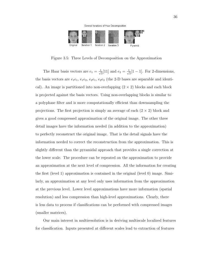
36
Figure 3.5: Three Levels of Decomposition on the Approximation
The Haar basis vectors are e1 = 1√2[11] and e2 = 1√
2[1 − 1]. For 2-dimensions,
the basis vectors are e1e1, e1e2, e2e1, e2e2 (the 2-D bases are separable and identi-
cal). An image is partitioned into non-overlapping (2 × 2) blocks and each block
is projected against the basis vectors. Using non-overlapping blocks is similar to
a polyphase filter and is more computationally efficient than downsampling the
projections. The first projection is simply an average of each (2 × 2) block and
gives a good compressed approximation of the original image. The other three
detail images have the information needed (in addition to the approximation)
to perfectly reconstruct the original image. That is the detail signals have the
information needed to correct the reconstruction from the approximation. This is
slightly different than the pyramidal approach that provides a single correction at
the lower scale. The procedure can be repeated on the approximation to provide
an approximation at the next level of compression. All the information for creating
the first (level 1) approximation is contained in the original (level 0) image. Simi-
larly, an approximation at any level only uses information from the approximation
at the previous level. Lower level approximations have more information (spatial
resolution) and less compression than high-level approximations. Clearly, there
is less data to process if classifications can be performed with compressed images
(smaller matrices).
Our main interest in multiresolution is in deriving multiscale localized features
for classification. Inputs presented at different scales lead to extraction of features

37
at different scales. The next chapter continues the discussion of multiresolution
with more focus on deriving and using multiresolution features in PCA-M.

CHAPTER 4PRINCIPAL COMPONENT ANALYSIS WITH MULTIRESOLUTION
4.1 Definition of PCA-M
In this section, we formally treat localization with PCA. PCA is briefly dis-
cussed in a context of representation and feature extraction. PCA-M is presented
as PCA with localized outputs. The localized outputs of PCA-M are structured to
provide a multiscale representation. The section ends with a formal definition of
principal component analysis with multiresolution.
4.1.1 Localization of PCA
Consider a set of K training images,
ΦTRAIN = {φ1(n), . . . , φk(n), . . . , φK(n)}.
The pixels of each image φk(n), are indexed by n ∈ S. Define,
xk(n) = φk(n)−K
∑
k=1
φk(n).
If the training images already have zero mean, then xk(n) = φk(n). Principal
component analysis has two stages, training and testing (verification). The first
stage derives a set of eigenvectors and eigenvalues, (ψm(n), λm), for the set of
training images. Denote the set of eigenvectors by Ψ,
Ψ = {ψ1(n), . . . , ψm(n), . . . , ψM(n)}.
As discussed earlier, the number of non-zero eigenvectors ,M, is the minimum of
the number of exemplars, K, or the number of components of each exemplar, N .
38

39
The training stage of PCA finds a mapping from a set of training images to a set of
eigenvectors,
ΦTRAIN −→ Ψ (4.1)
Equation 4.1 emphasizes that the eigenvectors and eigenvalues are characteristics of
a set of input images. Since the input images and the eigenvectors have the same
spatial index, the eigenvectors are also called eigenimages. Once trained, PCA
uses the eigenimages to decompose each new input onto a set of components. The
second stage of PCA is a mapping from an input image to a set of M output scalar
components,
xk(n) −→ {y1, . . . , ym, . . . , yM}k. (4.2)
Equation 4.2 shows that each input has a unique set of outputs (components).
Since the association from input to output is usually implicit, notation can be
simplified. Rewrite equation 4.2,
x(n) −→ {y1, . . . , ym, . . . , yM}. (4.3)
Each component is global since its value is calculated using all the pixels of the
input image,
ym = < x(n), ψm(n) > =∑
n∈S
x(n)ψm(n). (4.4)
The dependency of a global output on a specific input pixel is seen by differentiat-
ing equation 4.4,
∀ (n ∈ S) :∂
∂ x(n)(ym) = ψ(n). (4.5)
Output localization implies that an output is dependent only on a local set of
pixels. Consider a subregion of the pixels, A ⊂ S. A local output could be specified

40
by
∂∂ x(n)
(yLOCAL) =
ψ(n), n ∈ A
0, otherwise.(4.6)
Localization could arise naturally if some of the eigenvector components were zero,
ψ(n) = 0. PCA-M forces localization by explicitly manipulating equation 4.6.
Definition 4.1.1 Consider a set of N-dimensional inputs, x(n). The components
of each input are indexed by n ∈ S, where S = [1, . . . , N ]. Let A be a subset of
S such that A corresponds to a localized time interval if x(n) is a time signal, or
to a local region if x(n) is an image. Denote the subregion of an input by xA(n).
Let wA(n) be the corresponding eigenvector (eigenimage). A localized PCA-M
output is
yA =< xA(n),wA(n) >=∑
n∈A
xA(n)wA(n). (4.7)
PCA-MFEATURE
EXTRACTOR CLASSIFIERx
θ(x) ξ ( θ(x) )
kDATA CLASS
Figure 4.1: PCA-M for Classification
Before defining a localized eigenvector, we want to restate our goals for PCA-M so
that the design choices will be understood. First, both PCA and PCA-M provide
representations, but this does not mean that they can be automatically used
for feature extraction. In fact, PCA-M components are not directly constructed
for optimal discrimination. So PCA-M should be understood as a preprocessor
for classification that constrains the scale and locality of subsequent features
(Figure 4.1).
41
Second, given that PCA-M is not the ideal feature extractor, care should be
taken that no information is lost. Since PCA-M cannot identify whether some
information is needed for discrimination, all information should be propagated to
the classifier. PCA-M should (and can) provide at least a complete representation
of the input in the space of the training set. That is, some information from
non-training exemplars is always lost since the eigenspace is a subspace of all
possible inputs. If the application is classification, an overcomplete representation
(redundancy) is not only acceptable, but may be essential. Nonetheless, we design
PCA-M with a minimum amount of redundancy. It is usually much easier to add
redundancy than reduce redundancy.
Finally, in allowing each output to have inputs of varying geometry (scale and
shape), localized eigenvectors are not guaranteed to be orthogonal. Since they are
not orthogonal, it is an abuse of nomenclature to continue to refer to the localized
eigenvectors as “eigenvectors”. Since the PCA-M network weights converge to the
localized eigenvectors, we will henceforth call them PCA-M weights. Orthogonality
has a direct impact on designing PCA-M since many implementations of PCA
involve deflation in some form. While it is not always apparent from the network
architecture, there is an inherent sequencing of calculations. As the weights for
the first output are calculated, the weights and output are used to reconstruct an
estimated input. The input is deflated by the estimate, and the deflated inputs are
used as “effective inputs” for calculating the weights of subsequent outputs.
4.1.2 A Structure of Localized Outputs
Definition 4.1.1 is not an implementable definition for a localized PCA-M
output since the corresponding localized eigenvector wA(n) is not yet defined. If
all outputs are supported by the same region, the eigenvectors are found using
standard PCA with the localized input, xA(n), as the new input. If each output
is supported by a separate non-overlapping region, the localized eigenvector is

42
found by treating each region as a separate standard PCA problems. When the
outputs are localized to overlapping regions of varying geometry (size and shape),
the meaning of orthogonality becomes unclear. That is, eigenvectors that derived
from the same subregion of the training images are orthogonal. Also, eigenvectors
that are each derived from non-overlapping subregions are orthogonal. However,
eigenvectors that are each derived from partially overlapping subregions are not
generally orthogonal
Definition 4.1.2 Consider a set of N-dimensional inputs, x(n), with an associated
set of M eigenvectors, ψ(n). For both the inputs and eigenvectors, components are
indexed by n ∈ S, where S = [1, . . . , N ]. PCA-M is an iterative procedure:
1. For the first eigenvector, partition S into R(1) subregions such that
⋃
r∈[1...R(1)]
Sr = S, (4.8)
2. treating each subregion as a separate eigenvalue problem, calculate the first
eigenvector for each region,
3. deflate each region of the input, and use the deflated input as the effective
input for subsequent calculation.
The geometry of the partitions can change for each iteration. The number of
iterations to span the input space will not exceed M .
A global scalar output ym is replaced by an array of R(m) localized outputs,
ym = [y1 . . . yr(m) . . . yR(m)], (4.9)
where
yr(m) =∑
n∈A
xk(n)wm(n), where, A = Sr(m). (4.10)
Each array of outputs, ym, is a compressed version of the input image. A fine
partitioning (R(m) large) corresponds to a fine resolution for ym. If the partitions
43
are identical for each array of outputs ym, the representation has fixed resolution.
Analogous to equation 4.2, the mapping for PCA-M is
xk(n) −→ {ym(r(m))}k. (4.11)
The PCA network trains M sets of weights corresponding to full eigenimages. The
PCA-M network has (∑M
m=1 R(m)) sets of weights corresponding to partitioned
eigenimages. The PCA-M network replaces each scalar global output, ym, with an
array of localized outputs, ym. Constraints on the weights of the GHA network
allow control of the partitioning (number and composition) for each output.
Control of the structure of the partitions sets the localization and scale for the
PCA-M network.
4.2 The Classification Problem
The applications presented in the next chapter use PCA-M for classification.
This section restates the basic classification problem so that PCA-M can be
discussed in the context of feature extraction.
Given a choice of several classes Ck and some data xn, a basic classifier assigns
the input to one of the classes.
xn 7→ Ck.
Equivalently, the class index k is a function of the input x,
k = g(xn). (4.12)
For example, a classifier could identify that photograph xn belongs to person k.
Mathematically, designing a good classifier is finding a good mapping function
g. Each class of data contains features; that is, characteristics that are useful
for classification. Ideally those features, ϑ(x), could be separated from the “use-
less” characteristics in the raw data. Presented with only the pertinent data for

44
classification, the task of the classifier becomes easier.
k = f(ϑ(x)) = g(x). (4.13)
Worsening the resolution of the inputs is intended to remove details that are not
needed for classification, while retaining coarse features that are needed. In general,
too fine a resolution retains unneeded details, while too coarse a resolution discards
critical information. A multiresolution approach provides a structure for control
of the detailed information. PCA-M can provide multiscale representations of an
exemplar to allow extraction of features at different scales (section 4.3.3). PCA-M
can also be used to directly localize a global eigenimage (section 4.3.4). A search
for features in the universal space may not be feasible, but the eigenspace may
be too restrictive for feature extraction. PCA-M provides a space richer than
eigenspace (figure 4.2), but still keeps the dimensionality under control.
All Features
PCA-MFeatures
PCAFeatures
Figure 4.2: PCA and PCA-M in Feature Space
4.3 Complete Representations
The section on eigenfaces is a classical application of PCA to images. PCA can
be conceptualized as PCA-M with the coarsest partitioning (equation 4.8),
∀m : R(m) = 1.

45
The identity map is presented for contrast as PCA-M with the finest partitioning,
∀m : R(m) = N.
The iterated filter bank and dual decomposition have milder restrictions on the
partition sizes but implement constraints based on stationarity. The identity map
can be considered as PCA with fully localized outputs. The next section is an
example of PCA with global outputs. The subsequent section on iterated filter
banks describe a structure with outputs of varying localization.
4.3.1 Eigenfaces
The theoretical side of standard PCA has been discussed earlier. The eigen-
faces section presents an implementation of standard PCA using the generalized
hebbian algorithm (GHA) presented in section 2.5. Since the theory and struc-
ture has been discussed earlier, this section presents experimental results. The
PCA decompositions presented in this section are used for comparison to PCA-M
decompositions (in the next section) of the same set of data.
The GHA network is a simple, flexible and efficient way to implement PCA.
Minor structural modifications lead to multiresolution. This section presents the
GHA Network used for standard PCA. Subsequent sections then step through
several modifications. With each modification, we present:
1. the network structure,
2. the changes in the representation that arise from the modifications,
3. an example of the representation using one of the faces drawn from the ORL
database.
Figure 4.3 shows K = 10 pictures from the ORL database. These ten pictures
{φk}(k=1···10) are all of the same person and cropped to R = 112 rows and C = 92
columns.

46
Figure 4.3: Raw Images from ORL Database
Each input φk = φk(n) is described by two indices. The index k identifies the
specific exemplar, and the index n specified the specific component of φk. For time
signals, n is an one-dimensional index and the components are time samples. For
images, n specifies the row and column of the image’s pixels; n can be either a
two-dimensional vector index or an one-dimensional index to a rasterized version of
the image. The class average φ0 is formed by averaging the ten faces.
xk = φk −1K
(K
∑
k=1
φk) = φk − φ0.
After subtracting the average from each face, the residual images {xk}(k=1···10) are
shown in figure 4.4.
Figure 4.4: Residual Images for GHA Input
The residual images are each presented at the input layer of a network similar to
figure 4.5(left).

47
IN OUT IN OUT
Figure 4.5: Two single layer networks with: each output driven by all inputs (left),
and each output driven by single input(right)
The number of input nodes for the GHA network is determined by the dimensions
of the exemplars, 10304 = (112 × 92). The number of non-zero output nodes
can be no more than the number of linearly independent inputs; for this example,
there are ten output nodes. The network has a single computational layer with
every input connect to each output; each output has 10304 associated weights. For
convenience, construct the input matrix X = X(k, n) such that each input image
xk is a column of X,
X = [x1|x2| · · · |xK ]. (4.14)
As each exemplar is presented at the input layer, the output is calculated and the
weights are updated, using equations 4.15 and 4.16.
yj(n) =p−1∑
i=0
wji(n)xi(n), calculate output (4.15)
∆wji(n) = ηyj(n)
[
xi(n)−j
∑
k=0
wki(n)yk(n)
]
, update weights (4.16)
Equation 4.16 shows that each output is affected by prior outputs. This depen-
dency is shown in figure 4.5 (left) by dashed lateral connections between output

48
nodes. Since the training set had ten linearly independent images, the network
converges to ten sets of weights, {wk}k=1···10. The (10304 × 10) transformation
matrix WA is constructed by setting each wk as a column of WA,
WA = [w1|w2| · · · |w10]. (4.17)
The weights are eigenvectors that will be described by w = wk = wk(n) depending
on the context. The index k identifies the corresponding output nodes of the GHA
network. The ordering for GHA output nodes orders the eigenvectors such that the
corresponding eigenvalues are in decreasing order. Each wk has 10304 components
that can be arranged in an (112 × 92) array corresponding to the positions of
the associated input components. When the eigenvectors are arranged as a two-
dimensional array, the eigenvectors are also called eigenimages. The eigenimages
resemble the input faces. Because of this resemblance, the eigenvectors are also
called eigenfaces.
Figure 4.6: Eigenfaces from GHA Weights
Possibly the widest application for PCA is in signal representation and reconstruc-
tion. The training inputs can be perfectly reconstructed as a linear combination of
eigenfaces. The quality for reconstruction of other inputs depends on the degree
that the exemplars are representative of other inputs. The eigenvalues are an
indication of the reduction in reconstruction MSE. Table 4.1 shows that the inputs
can be reconstructed with about 10% reconstruction error using just the first four
eigenfaces and that the contribution from the last eigenface is negligible.

49
Table 4.1: Normalized Eigenvalues
λ1 23.90% λ6 5.83%
λ2 21.74% λ7 4.02%
λ3 19.26% λ8 3.64%
λ4 10.63% λ9 3.03%
λ5 7.92% λ10 0.00%
The eigenface expansion provides reconstruction for the network inputs. The inputs
are the residual images (exemplars minus the average image). The reconstruction
of the original exemplars requires adding back the class average. Because the PCA
analysis characterizes residual images, it is expected that the average image is
poorly reconstructed by eigenvalue expansion. This is especially interesting since
most of the energy is in the average image (table 4.2). In a classification problem,
there is an average image for each class as well as a single average for all images
across all classes. The high energy in the individual class averages suggests that
each class is characterized by the variation of its class average from the overall
average, not by the variations in the individual images.
Table 4.2: Energy Distribution of Exemplars
Energy in Energy in Percent inExemplar Average Component Componentx1 0.2970 0.0150 4.81%x2 0.3614 0.0212 6.80%x3 0.3130 0.0166 5.32%x4 0.3454 0.0154 4.95%x5 0.3492 0.0114 3.66%x6 0.3419 0.0168 5.40%x7 0.3155 0.0099 3.19%x8 0.3034 0.0122 3.92%x9 0.3243 0.0153 4.93%x10 0.3126 0.0144 4.65%Avg 0.3264 0.0148 4.76%

50
4.3.2 Identity Map
Some properties of the standard GHA network are more evident when con-
trasted to another network. This section provides a subjective discussion of the
following modifications to the standard GHA network:
1. the number of output nodes,
2. the dependencies (lateral connections) between output nodes,
3. the number and selection of inputs to an output node.
Since the key modification of PCA-M involves controlling the inputs scale to
an output node, it is instructive to examine the extreme case of a single output
for each input. This structure can be realized with a network that has all inputs
connected to each output, but with the constraint that only one weight is non-zero.
The network is shown in figure 4.5 (right) showing only the non-zero connections.
The inputs (figure 4.4) have not changed, so there are still 10304 input nodes
corresponding to the dimensions of the input exemplars. By design, there are also
10304 output nodes to provide an output for each input. Each output node has
the same spatial localization as the corresponding input node. This architecture is
actually 10304 independent GHA networks operating independently so the number
of outputs does not exceed the number of linearly independent exemplars.
Without loss of generality, stipulate that the final weights are normalized.
Construct the (10304× 10304) transformation matrix W1,
W1 = [w1|w2| · · · |w10304]. (4.18)
It should be evident that the transformation matrix W1 is a (10304 × 10304)
identity matrix.
The transformation matrices from equations 4.17 and 4.18 provide insight to
several key consequences of partial connections.
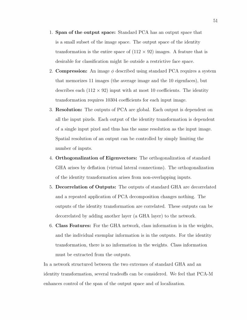
51
1. Span of the output space: Standard PCA has an output space that
is a small subset of the image space. The output space of the identity
transformation is the entire space of (112 × 92) images. A feature that is
desirable for classification might lie outside a restrictive face space.
2. Compression: An image φ described using standard PCA requires a system
that memorizes 11 images (the average image and the 10 eigenfaces), but
describes each (112 × 92) input with at most 10 coefficients. The identity
transformation requires 10304 coefficients for each input image.
3. Resolution: The outputs of PCA are global. Each output is dependent on
all the input pixels. Each output of the identity transformation is dependent
of a single input pixel and thus has the same resolution as the input image.
Spatial resolution of an output can be controlled by simply limiting the
number of inputs.
4. Orthogonalization of Eigenvectors: The orthogonalization of standard
GHA arises by deflation (virtual lateral connections). The orthogonalization
of the identity transformation arises from non-overlapping inputs.
5. Decorrelation of Outputs: The outputs of standard GHA are decorrelated
and a repeated application of PCA decomposition changes nothing. The
outputs of the identity transformation are correlated. These outputs can be
decorrelated by adding another layer (a GHA layer) to the network.
6. Class Features: For the GHA network, class information is in the weights,
and the individual exemplar information is in the outputs. For the identity
transformation, there is no information in the weights. Class information
must be extracted from the outputs.
In a network structured between the two extremes of standard GHA and an
identity transformation, several tradeoffs can be considered. We feel that PCA-M
enhances control of the span of the output space and of localization.

52
4.3.3 Iterated Filter Banks
The eigenface decomposition and the identity map may be considered as two
extreme cases of fixed resolution PCA. The iterated filter bank structure is the
first multiresolution network presented in this chapter. The iterated filter bank is
also of interest since it is a way of implementing PCA-M for a complete represen-
tation. The concepts follow from prior sections and the focus is in describing the
architecture and constraints.
Allowing partial connections makes it possible to arbitrarily assign inputs
to outputs and control orthogonality between outputs. The number of possible
networks increases dramatically. For example, if each output is connected to two
inputs there are C(n, r) = C(10304, 2) = 53081056 unique combinations of
inputs. For each pair of inputs there are two orthogonal outputs, so it is possible to
construct a network with over 108 orthogonal outputs.
IN
N1(2)
N2(2)
N3(2)
N4(2)
N5(4)
N6(4)
N7(8)
N8(8)
OUT
HH1 2 ↓
HL1 2 ↓HH2 2 ↓
HL2 2 ↓HH3 2 ↓
HL3 2 ↓
N7
N8
N1−4
N5−6
HH1
HL1
HH2
HL2
HH3
HL3
HH1
HL1(2 ↑ HH2)
HL1(2 ↑ (HH2(2 ↑ HL3)))
HL1(2 ↑ (HH2(2 ↑ HH3)))
2 ↓
4 ↓
8 ↓
8 ↓
N1−4
N5−6
N7
N8
Figure 4.7: Three Level Dyadic Banks
One possible structure mimics the structure of a dyadic filter bank. The
structure of a three level dyadic bank is shown on the top left of figure 4.7 with
the equivalent polyphase construction on the bottom right. The filters used in
this example are constrained to be two tap FIR filters. The filters are derived

53
from the eigenvectors of the (2 × 2) scatter matrices of the data at each stage.
Four sequential outputs of the first filter correspond to the outputs at the first
four nodes (N1 − 4) of the network. Two sequential outputs of the second filter
correspond to the outputs at the fifth (N5) and sixth (6) nodes of the network.
The GHA network iterates on the lowest energy (variance) component. For inputs
that have 1/f energy distributions, the lowpass or highpass components can be
selected by using Hebbian or anti-Hebbian learning for the output node.
The network (figure 4.7 left) has four nodes (N1 − 4) that are each connected
to two non-overlapping contiguous inputs. The numbers of connected inputs are
in parenthesis after the node labels. Output nodes N5 − 6 are each connected to
four contiguous non-overlapping inputs, and the last two nodes N7 − 8 are fully
connected. The weights of N1−4 are constrained to be equal since they correspond
to a single filter in the filter bank. For the same reason, the weights for outputs
N5− 6 are constrained to be equal.
GHA orthogonalizes weights by deflating the inputs to subsequent output
nodes. Deflation is ineffective for non-overlapping inputs. The first four nodes have
no orthogonalization constraints from other nodes. Node N5 is directly affected
only by nodes N1− 2 since the inputs of those two nodes are partitions of the input
to N5. Node N6 is directly affected only by nodes N3− 4 (indirectly influenced by
N1− 2 because of the equality constraint between N5 and N6). The weights of the
fully connected outputs N7−8 are constrained by all earlier nodes. The three-stage
dyadic (twofold) bank produces eight outputs for each set of eight inputs.
For the ORL images, a quadratic (fourfold) filter was used. At each stage the
inputs were partitioned into non-overlapping (2× 2) blocks. To parallel the dyadic
filter bank, all regions are constrained to have the same weights. The scatter

54
matrix of the first stage inputs is
S =
0.99 0.95 0.91 0.90
0.95 1.00 0.89 0.93
0.91 0.89 1.00 0.95
0.90 0.93 0.95 1.01
(4.19)
Due to the local nonstationarity of images, the autocorrelations differ by mode
(horizontal, vertical, diagonal) as well as by lag. The scatter matrix is doubly
symmetric but not (in general) Toeplitz. The first four eigenvectors are shown in
figure 4.8 and show that the filter is essentially separable along the horizontal and
vertical modes.
Figure 4.8: The first four (2 × 2) eigenimages are separable odd-even decomposi-
tions. From left to right: even horizontal and vertical (λ1 = 0.9415), odd horizontal
and even vertical (λ1 = 0.0346), even horizontal and odd vertical (λ1 = 0.0183),
odd horizontal and vertical (λ1 = 0.0056)
The weights (features) are separable even (low-pass) and odd (high-pass) decom-
positions. Figure 4.7( bottom-right) shows that the iterated filter bank develops
longer filters by cascading shorter filters. Short eigenfilter coefficients are driven by
PCA symmetry constraints and cannot adapt to data statistics.
Figure 4.9 (top) shows the outputs of three stages. For display purposes, each
image was normalized so that pixel intensities lie in the range (0, 1). The first
stage of the filter bank produces four outputs shown in the four top left panels of
figure 4.9. The four images are downsampled and arranged as a (2 × 2) array of
compressed images as shown in the top right panel. There is no implied ordering

55
or spatial relationship in the arrangement of the compressed images. We place the
compressed image to be iterated in the top-left of the (2 × 2) array. The low-pass
component (top-left) is passed to another iteration. The downsampled outputs of
the second stage are shown in the bottom, far left panel. The panel is displayed at
double scale. The third stage outputs are shown in the bottom, middle left panel
the figure 4.9. The (2× 2) array of outputs from the third stage output is displayed
at four times the actual scale. The outputs of all three stages are combined in the
bottom middle image. For comparison, the residual (original minus average) and
the original image are shown on the bottom right.
Figure 4.9: Three Level Decomposition of an Exemplar Face
The first stage outputs of all ten inputs are shown in figure 4.10.
Figure 4.10: Output of the First Stage of the Quadratic Filter Bank for the Ten
Training Exemplars
A large disadvantage of the iterated filter bank is limited adaptability:

56
1. Short Filter Length Constraint The weights cannot adapt to class
statistics (no global feature extraction).
2. Equal Weight Constraint The weights are constrained to be the same for
all subimages (no localization of features).
The chief advantage of the iterated filter bank is that an orthogonal basis is used
at each stage. The overall linear transformation is orthogonal and guarantees
perfect reconstruction of the inputs. The iterated filter bank structure produces a
multiresolution representation at the output. If the compressed representations are
difficult to classify, then feature extraction must be implemented by another stage.
4.3.4 Dual Implementation of PCA
The filter bank structure first extracts small highly localized features, then
builds up to global features. Another alternative is to find global features before
local features. In general, it cannot be guaranteed that the resulting localized
eigenvectors will form a minimal spanning set. That is, while we can still guarantee
a set of vectors to span the space of training exemplars, PCA-M might not produce
a minimal spanning set. As previously mentioned, a minimal spanning set is not
required and perhaps not desired for classification. If the process is wide-sense
stationary (WSS), then the network weights form a pair-wise linearly independent
set of vectors. The discussion of orthogonal bases will be deferred to the next
section.
The behavior of PCA-M in going from long filters to short filters is clearer
when discussed in the context of the dual PCA decomposition. PCA can be done
using the transpose of the data matrix X ( 4.14). The main consideration is that
the number of exemplars is usually much smaller than the dimension (number of
components) of an input. The dual scatter matrix is
SD = X ′X. (4.20)

57
Continuing with the ORL example, the original scatter matrix is a doubly sym-
metric (10304 × 10304) matrix. The dual scatter matrix is a (10 × 10) matrix.
An analytic solution to PCA has operations in the order of O(N2), so there is a
significant computational advantage to using the dual PCA.
Standard Dual
S=XX ′ SD=X ′X
XX ′=WΛW ′ X ′X=V ΛV ′
XX ′W=WΛ(W ′W ) X ′XV =V Λ(V ′V )
XX ′W=WΛ1 X ′XV =V Λ1
X ′XX ′W=X ′WΛ XX ′XV =XV Λ
X ′X(X ′W )=(X ′W )Λ XX ′(XV )=(XV )Λ
V =X ′W W=XV
(4.21)
Equation 4.21 contrasts the standard decomposition S = WΛW ′ to the dual
decomposition SD = V ΛV ′. The dual eigenvalues are equal. The eigenvectors W
can be calculated from the dual eigenvector V ,
W = XV. (4.22)
The columns of the matrix W are orthogonal but not orthonormal. Normalizing W
results in W .
The dual formulation can significantly reduce computations when the number
of exemplars is smaller than the spatial dimension of the exemplars. The formu-
lation also provides an alternative interpretation to PCA-M. Consider a single
exemplar x1, and a single eigenface w1 (equation 4.17). Partition each array,
x1 =
x1,(1,1) x1,(1,2)
x1,(2,1) x1,(2,2)
w1 =
w1,(1,1) w1,(1,2)
w1,(2,1) w1,(2,2)
. (4.23)
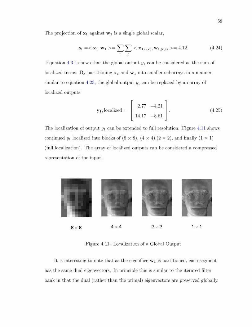
58
The projection of x1 against w1 is a single global scalar,
y1 =< x1,w1 >=∑
r
∑
c
< x1,(r,c),w1,(r,c) >= 4.12. (4.24)
Equation 4.3.4 shows that the global output y1 can be considered as the sum of
localized terms. By partitioning x1 and w1 into smaller subarrays in a manner
similar to equation 4.23, the global output y1 can be replaced by an array of
localized outputs.
y1, localized =
2.77 −4.21
14.17 −8.61
. (4.25)
The localization of output y1 can be extended to full resolution. Figure 4.11 shows
continued y1 localized into blocks of (8 × 8), (4 × 4),(2 × 2), and finally (1 × 1)
(full localization). The array of localized outputs can be considered a compressed
representation of the input.
Figure 4.11: Localization of a Global Output
It is interesting to note that as the eigenface w1 is partitioned, each segment
has the same dual eigenvectors. In principle this is similar to the iterated filter
bank in that the dual (rather than the primal) eigenvectors are preserved globally.

59
The meaning of the variations across exemplars was not explored since the vari-
ations seem to arise from misalignment during data collection rather than from
an inherent feature of the class. Although multiresolution can be easily extended
to standard PCA by simply partitioning the standard eigenvectors, the repre-
sentations that result are always overcomplete. An overcomplete representation
contains redundancy that is a disadvantage if the application is to compactly
transmit information. For classification, an overcomplete representation may be
advantageous.
4.4 Overcomplete Representations
The preceding section showed two ways that PCA-M could be constrained
to produce complete or overcomplete representations. For the iterated bank, the
weights for each partition were constrained to be equal. In the dual approach, the
statistics over the entire image were assumed stationary. For classification, features
are important and overcomplete representations are satisfactory. In this section the
flexibility of the single layer GHA network is discussed.
The single computational layer GHA network outputs are determined by the
inputs. There are three main mechanisms for controlling the input,
1. control deflation from other outputs,
2. mask all inputs outside a selected region,
3. place explicit constraints in the training.
The original algorithm is to provide deflated inputs to successive outputs. For fixed
resolution PCA, the deflation is needed to prevent different outputs from having
weights converge to the same values. For multiresolution, the deflated inputs are
only required if the input nodes are identical, otherwise deflation is optional. By
selectively constraining weights to zero, an output can be localized to subregions of
arbitrary size and shape. The subregions need not be convex or connected (e.g., a
region for both eyes but excluding the nose). Each subregion of the image can be of

60
a different size and shape. Overlapping regions are allowed to reduce edge effects.
Shifted outputs can be introduced to facilitate shifts (translations) in the image.
Each partition is allowed to have different statistics and allowed to converge to a
local subeigenimage.
Relaxing all the constraints produce a richer set of characteristics. Relaxing
constraints also complicates the implementation. The specific choices for a PCA-M
network are discussed in the experiments. The overall approach, however, was to
relax a single constraint at a time until the network’s classification performance was
adequate.
4.5 Local Feature Analysis
Penev and Atick (1996) report great success in face classification using a
technique called Local Feature Analysis(LFA). The improvement in performance is
attributed to localized feature extraction. Atick has also implemented a commercial
automated face classification program, (FaceIt, http://venezia.rockefeller.
edu/group/papers/full/AdvImaging/index.html) for workstations using LFA.
PCA/SVD LFA
LFAMAPPER
Ensembleof Inputs
SingleInput,φk(n)
Eigenvectors,Ψ(n,m)Eigenvalues,Λ
K(n,m)P(n,m)
SingleOutput,Ok(n)
Figure 4.12: Local Feature Analysis
Figure 4.12 shows that LFA is based on PCA. The top cascade of operations
calculates class properties. The bottom row is the LFA mapper proper. Assume
a set of K inputs, φk(n), which are exemplars of a single class. Each input has a
spatial dimension n that can be rasterized such that 1 ≤ n ≤ N . For the ORL faces
N is equal to the number of pixels in each input, N = (R×C) = 10304. PCA is the

61
eigenvalue decomposition of inputs’ scatter matrix S(N×N). In general, eigenvalue
analysis yields a square modal matrix Ψ(N×N)(n1, n2) and a single diagonal matrix
of eigenvalues Λ. The eigenvalue decomposition produces K eigenvectors, but only
the first M eigenvectors are retained (M < K � N). The truncated expansion
uses eigenvectors ψm(n) with corresponding eigenvalues λm. The modal matrix
is not square since the number of linearly independent inputs K is less than the
dimension N . Since M < K � N , the modal matrix Ψ(n1, n2) is (N ×M). Using
the eigenvectors as a basis, each input can be reconstructed,
φk(n) =K
∑
m=1
Amψm(n),
φk(n) =M
∑
m=1
Amψm(n).
LFA introduces some new quantities that will be discussed in more detail in
separate subsections,
O(n) ,∑M
m=11√λm
Amψm, Output vectors,
K(n1, n2) ,∑M
m=1 ψm(n1) 1√λmrψm(n2), LFA kernel,
P (n1, n2) ,∑M
m=1 ψm(n1)ψm(n2), Residual Correlation.The LFA kernel K(n1, n2) is a topographic (Penev and Atick, 1996, p. 5) analog
for the modal matrix. The residual correlation P (n1, n2) is comparable to the
matrix of eigenvalues Λ. The LFA output is similar to the reconstructed input in
PCA.
4.5.1 Output Vector
Using the LFA kernel, an output O(n) is computed for every input φ(n),
O(n1) =∫
K(n1, n2)φ(n2) =M
∑
m=1
1√λm
Amψm (4.26)
The output O(n) is of the same dimension as the input φ(n). The LFA output is
the PCA reconstruction except that each eigenvector is normalized (scaled to unit

62
norm),
< ψm, ψl >= λmδ(m,l) −→ < 1λm
ψm, 1λl
ψl >= δ(m,l). (4.27)
For convenience, the expressions for input and output are repeated here,
φ(n) =M
∑
m=1
Amψm (4.28)
O(n) =M
∑
m=1
Am1√λm
ψm (4.29)
The main difference (between a PCA reconstruction and an LFA output) seems
to be that normalizing the eigenvectors the scale factor de-emphasizes terms
with large eigenvalues in equation 4.28. In PCA, these are the terms that are the
most important for reconstructions with minimum mean squared error (MSE).
On the other hand, it has also been suggested that eliminating the first principal
components (that are the low frequency components in “natural” (1/f) images) can
compensate for differences in illumination level. The objection to discarding the
first few principal components is that essential discriminatory information may be
lost. LFA’s approach of de-emphasis rather than outright elimination of the first
eigenvectors may provide features that are robust with respect to illumination.
4.5.2 Residual Correlation
The residual correlation matrix definition can be rewritten in matrix form,
P (n1, n2) ,∑M
m=1 ψm(n1)ψm(n2),
=∑K
m=1 ψm(n1)ψm(n2)−∑K
m=M+1 ψm(n1)ψm(n2),
= ΨΨ′ −∑K
m=M+1 ψm(n1)ψm(n2),
= 1−∑K
m=M+1 ψk(n1)ψk(n2).
(4.30)
If the full set of K eigenvectors is used for LFA output expansion, then the residual
correlation of the output is the identity matrix. If only a subset M < K of the

63
eigenvectors is used, there is a residual correlation as shown in equation 4.30. Atick
and Penev note that the LFA output correlations “happen to be” localized.
4.5.3 Kernel
The scatter matrix of the input data can be rewritten,
ΦΦ′ = ΨΛΨ′
=∑K
m=1 λmψm(x)ψm(x)′(4.31)
Writing the expressions for the scatter matrix and the inverse kernel together,
ΦΦ′ =∑K
m=1 λm ψm(n1)ψm(n2)′
K−1 =∑M
m=1
√λm ψm(n1)ψm(n2)′
(4.32)
The inverse kernel is comparable to the original scatter matrix except for the
number of terms (M < N), and the scale factor. The key difference in LFA seems
to be the scaling by√
λm, otherwise, the analysis is similar to a partial PCA
reconstruction.
4.5.4 LFA on ORL Faces
The ORL database has ten exemplars of each person. K = 9 exemplars were
used for training and one retained for evaluating the expansion. Figure 4.13 shows
normalized (by input image power) reconstruction MSE as a function of number of
components. The starting MSE (at x = 0) is from just using the average image.
Each of the lines is for a different input φm.

64
Figure 4.13: PCA Reconstruction MSE
Figure 4.14 shows the reconstruction φr(x) using only the M = 8 eigenvectors
corresponding to the eight largest eigenvalues. Note that the poses that are not
fully frontal have artifacts, the reconstructions using M = 9 are indistinguishable
from the inputs. The error from adding the tenth component is an artifact incurred
by implementation limitations on numerical accuracy.
Figure 4.14: PCA Reconstructions
Figure 4.15 shows the corresponding LFA outputs,

65
Figure 4.15: LFA Outputs (Compare to PCA Reconstruction)
The kernel and residual correlation matrices each have 106, 172, 416 =
(10, 304 × 10, 304) ≈ 108 elements. Each row of the kernel is a sum of scaled
PCA eigenfaces. Penev and Atick (1996) shows that local features can be found
from an appropriate linear combination of global features. What conditions are
needed so that an arbitrary image (e.g., a local feature) can be reconstructed using
eigenimages (global features)? Clearly, the local feature must be contained in the
span of the eigenspace. The span of the eigenspace is dependent on the number of
independent training exemplars. That is, as the number of independent training
exemplars increases, the span of the eigenspace increases. Figure 4.16 shows the
first five rows, each row reshaped to a (112 × 92) image of the LFA Kernel (top
row) and Residual Correlation (bottom row),
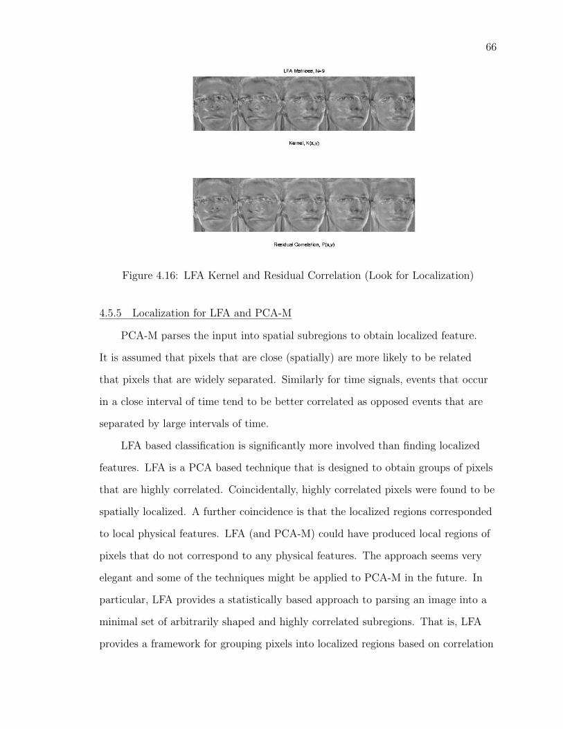
66
Figure 4.16: LFA Kernel and Residual Correlation (Look for Localization)
4.5.5 Localization for LFA and PCA-M
PCA-M parses the input into spatial subregions to obtain localized feature.
It is assumed that pixels that are close (spatially) are more likely to be related
that pixels that are widely separated. Similarly for time signals, events that occur
in a close interval of time tend to be better correlated as opposed events that are
separated by large intervals of time.
LFA based classification is significantly more involved than finding localized
features. LFA is a PCA based technique that is designed to obtain groups of pixels
that are highly correlated. Coincidentally, highly correlated pixels were found to be
spatially localized. A further coincidence is that the localized regions corresponded
to local physical features. LFA (and PCA-M) could have produced local regions of
pixels that do not correspond to any physical features. The approach seems very
elegant and some of the techniques might be applied to PCA-M in the future. In
particular, LFA provides a statistically based approach to parsing an image into a
minimal set of arbitrarily shaped and highly correlated subregions. That is, LFA
provides a framework for grouping pixels into localized regions based on correlation

67
rather than simple adjacency. Further, LFA provides a nice verification that, for
faces, spatially localized features are well correlated.
4.5.6 Feature Space for LFA, PCA, and PCA-M
For a given set of input exemplars, LFA and PCA have the same feature
space. To derive local features, both PCA and LFA rely on the eigenspace having
a sufficiently large span so that local features are included. In both PCA and
LFA, the eigenspace can only be increased by using more (linearly independent)
training exemplars. That is, LFA localized features are a linear combination of
a large number of training exemplars. Kirby and Sirovich (1987) estimates that
a dimensionality of at least 400 is needed for adequate representation of tightly
cropped faces with PCA. Penev (1999) states that a dimensionality of 200 (at
least 200 exemplars) is needed for adequate representation of faces with LFA.
In the ORL example, with only nine exemplars of (112 × 92) images, any linear
combination will be “face-like” and not localized.
PCA-M is a multiresolution technique that encompasses classical PCA as an
extreme case within the PCA-M definition. PCA-M directly manipulates local-
ization by partitioning the exemplar images. PCA-M then adapts to the second
order statistics in each localized region. Localization of features is independent
of the number of training exemplars. Further, PCA-M facilitates construction of
multi-scale features. That is, PCA-M can be utilized with global features as well as
(local) features of varying scale.
4.6 Summary
PCA-M can be used to directly derive features for classification. Local
features can be found by explicitly selecting regions that correspond to local
physical structures. Unfortunately, there is often no a priori way to know that
the best mathematical features correspond to given physical features. If a priori

68
information is available, the GHA network can structure the PCA-M network in
a very flexible manner. Unlike LFA which looks for local features by exhaustive
linear combinations of global features, PCA-M can explicitly selecting regions that
correspond to local physical structures.
PCA-M seems to be sufficiently useful in providing localized inputs to an-
other classifier such as a neural network. The neural network can then choose to
construct features that are global or local. The classifier can create features that
are combinations of PCA-M outputs at a single scale, or combine PCA-M outputs
of several scales. The subsequent experiments showed that a single layer PCA-M
network followed by a single layer classifier performed comparably or better than
more complicated structures.
CHAPTER 5FACE RECOGNITION EXPERIMENT
In recent years, automated face recognition has received increased interest
while simultaneously becoming more feasible. Surveillance and medical diagnostics
are two broad classes of applications that have driven the demand for image
recognition technology. Hardware for image recognition has shown a trend towards
higher performance, increased accessibility, and lowered costs. Numerous advances
have been made in face recognition algorithms (Chellappa et al., 1995, pp. 705 -
706).
Automated face recognition and classification has many practical applica-
tions (Chellappa et al., 1995, p. 707). In general, automated face recognition is
a complex problem that requires detecting and isolating a face under unknown
lighting conditions, backgrounds, orientations, and distances. However, there are
several applications where the lighting, scale, and background can be expected to
be well controlled:
• personal identification (credit cards, passports, driver’s license),
• mug shot matching,
• automated store/bank access control.
In these applications, detection and isolation of the faces is not necessary, Non-
linear distortions in the images (due to lighting, background, centering, scaling, or
rotation) can be controlled during data collection (and assumed to be negligible).
Chellappa et al. (1995) presents a nice survey that includes background
material on psychology and neuroscience studies, face recognition based on moving
video, and face recognition using profile faces. The scope of this dissertation
69

70
is limited to automated face recognition based on frontal, still photos. Given a
database of exemplar images, the basic face recognition problem is to identify
individuals in subsequent images. The performance expectations for automated
face recognition are high since most people can recognize faces despite fairly
adverse conditions. For a machine, the task involves detecting faces from a
cluttered background, isolating each face, extracting features from each face,
and finally classification of the face.
This chapter includes an extended presentation of three specific classifiers:
the original eigenfaces experiment, a Hidden Markov Model, and a convolutional
network. All three techniques have been applied to the same (Olivetti Research
Lab) face database under similar conditions. Finally, the PCA-M classifier is
presented against the same ORL database.
5.1 ORL face Database
Olivetti Research Lab (ORL) has a public face database reproduced in
appendix B. The database has 400 pictures made up from 10 pictures of 40 people.
The images are (112 × 92) = 10304 pixel, 8-bit grayscale images. The images
in the ORL database present a non-trivial classification problem. The pictures
show variation in background lighting, scale, orientation, and facial expression
(figure 5.1). The tolerance in scale is about 20% and the tolerance for tilting is
about 20◦ (Giles et al., 1997). Individuals who used eyeglasses were allowed to pose
both with and without eyeglasses. Some people looked very similar to each other
(figure 5.1, far right).

71
Figure 5.1: Varying Conditions in ORL Pictures
Several other techniques have been applied to the ORL database under the
same testing conditions (40 people, 5 test + 5 verification pictures for each person).
Control of the conditions is important since reducing the number of classes (not
using all 40 people) implies an easier classification problem. Changing the ratio of
training exemplars to verification exemplars also alters classifier performance. This
section discusses the three experiments that are used for comparison to PCA-M.
PCA-M gave better average performance than the other techniques.
Table 5.1: Error Rates of Several Algorithms
Algorithm PerformanceEigenfaces (Turk and Pentland, 1991a) 10%HMM (Samaria, 1994) 5.5%SOM-CN (Giles et al., 1997) 5.75% (3.8%)PCA-M (Brennan and Principe, 1998) 2.5%
5.2 Eigenfaces
The decomposition of a training set of face images into eigenfaces has been
previously discussed. This section briefly presents the face recognition experiment
using eigenface.

72
5.2.1 Description of Experiment
The ORL database has 200 training images, 5 images for each of the 40 people.
All the training images {Φk}1≤k≤200 are averaged,
Φ0 =1
200
200∑
k=1
Φk (5.1)
The ensemble average is removed from each image,
xk = Φk − Φ0. (5.2)
Eigenfaces Ψm are found for the training ensemble and M eigenfaces with signif-
icant eigenvalues are retained. The eigenfaces define the axes in eigenspace, and
both training and test images can be mapped to a set of coordinates in eigenspace,
xk → [α1, α2, . . . , αM ]k , where, αm =< x, Ψm > . (5.3)
Denote the eigenspace coordinate vector by ak = [α1, . . . , αM ]k. An immediate
advantage of eigenfaces is a steep reduction in dimension. For the ORL database
and using all the eigenfaces (M = 200), each image is described by 200 coordinates
rather than (92 × 112) = 10304 pixels. The training images can be compressed by
a factor of 50 without loss. The training images from each class map to separate
regions in eigenspace.
The eigenspace coordinates can be treated as raw input to any classifier. For
example, let the coordinates of the 5 training images from class n be denoted by
ank . The distance of a test image’s coordinates from the training image coordinates
for a class can be used to determine the probability of the test image belonging to
the class,
Prob(xtest ∈ n) = f(atest, an1 , . . . , a
n5 ). (5.4)

73
The simplest method is to average the coordinates of all the training exemplars
for a class, and to calculate the distance of a test image from the average coor-
dinates (Turk and Pentland, 1991b; Giles et al., 1997). Samaria (1994) used a
nearest-neighbor classifier.
5.2.2 Results
Pentland et al. (1994) reports under 05% error rate on 200 faces using a large
(unspecified) database. Samaria (1994) reported a 10% error rate when using 175
to 199 eigenfaces. The improvement after 10 eigenfaces is gradual, but the error
rate rapidly becomes worse when less than 10 faces are used. Samaria’s results also
showed that error rate was not monotonically non-increasing as the classifier used
more eigenfaces. Giles et al. (1997) reports a 10.5% using 40 to 100 eigenfaces.
Error rates aside, the eigenface approach demonstrates that PCA is a useful
preprocessor for classification.
1. PCA coordinates in eigenspace are good features for classification.
2. PCA reduces the dimensionality of the classifier inputs that in turn reduces
computations.
3. Eigenvalues are potentially a good indicator for classification features.
5.3 Face Recognition using HMM’s
Samaria (1994) on face recognition using a Hidden Markov Model (HMM)
is often cited as seminal work in applying statistical signal processing to image
classification. Hidden Markov Models are widely applied to continuous speech
recognition (Haykin, 1994, p. 227). Samaria passed an observation window over
an image from left-to-right, down, right-to-left, down, left-to-right, and so on
(Figure 5.2, left).

74
window
general traversal
window
top-down traversal
Figure 5.2: Parsing an Image into a Sequence of Observations
That is, an observation window traverses a one-dimensional path through each
image. For each image, Samaria thus obtained a corresponding observation array,
O = [o1, . . . ,oT].
5.3.1 Markov Models
A Markov model is a statistical model for a sequence of observations based
on an underlying sequence of states (a Markov process). The probability of a
state at some time in a sequence is dependent only on the immediately preceding
state (Therrien, 1992, pp. 99 - 118). Each transition between states generates an
output that is dependent only on the state being entered. If the states can be only
one of N countable discrete values, the process is called a Markov Chain (Therrien,
1992, pp. 99 - 118). The Markov process is described by four parameters (Samaria,
1994, p. 28),
1. the number of states N ,
2. the one-step state transition matrix, A = {ai,j : 1 ≤ i, j ≤ N},
3. the output probability function, B = {bj(.) : 1 ≤ j ≤ N},
4. the initial state probability distribution, Π = {πj : 1 ≤ j ≤ N}.
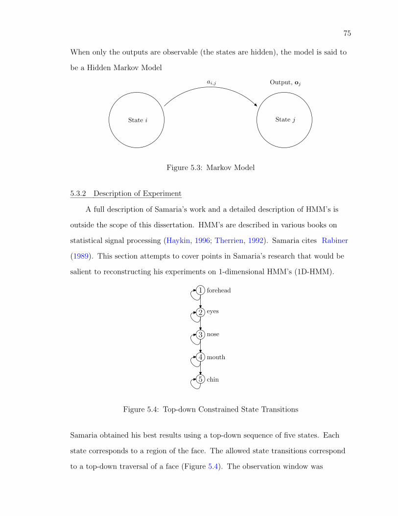
75
When only the outputs are observable (the states are hidden), the model is said to
be a Hidden Markov Model
State i State j
Output, ojai,j
Figure 5.3: Markov Model
5.3.2 Description of Experiment
A full description of Samaria’s work and a detailed description of HMM’s is
outside the scope of this dissertation. HMM’s are described in various books on
statistical signal processing (Haykin, 1996; Therrien, 1992). Samaria cites Rabiner
(1989). This section attempts to cover points in Samaria’s research that would be
salient to reconstructing his experiments on 1-dimensional HMM’s (1D-HMM).
1
2
3
4
5
forehead
eyes
nose
mouth
chin
Figure 5.4: Top-down Constrained State Transitions
Samaria obtained his best results using a top-down sequence of five states. Each
state corresponds to a region of the face. The allowed state transitions correspond
to a top-down traversal of a face (Figure 5.4). The observation window was

76
constructed from several complete rows of the image (Figure 5.2, right). Each
window was eight rows high and overlapped adjacent windows by seven rows.
Samaria described his model using a shorthand notation (Samaria, 1994, p. 42) of
H = (N (states) , L (observation rows) ,M (overlap rows) ) = (5, 8, 7)
Samaria used the HTK software package described in Young (1993). For each of
the 40 classes in the ORL database, five training images are each transformed into
a sequence of observations using a top-down traversal. The five training sequences
used as inputs to the HTK software with a design specification for five states (five
face regions). The HTK software derived optimal parameters for each HMM using
the Baum-Welch re-estimation algorithm (Baum, 1972). The optimization includes
parsing the training images into five regions, and deriving both the state transition
matrix A and output probability function B for the HMM. At the end of training,
an HMM has been derived for each class. To classify a test image, select the class
whose HMM maximizes the likelihood of the test image.
5.3.3 Results
Samaria’s dissertation exhaustively explored variations in the number of mod-
els, and observation window parameters. The dissertation included experiments
using frequency domain representations and reduced (spatial) resolution images.
Samaria reports that 1D-HMM outperformed the Eigenfaces approach about 40%
of the time. The 1D-HMM had an average error rate of 10%. After all the detailed
analysis, Samaria modestly concluded that the improvements (over eigenfaces) in
face recognition using 1D-HMM were probably not statistically significant. The
dissertation also explored a more complicated model, the P2D-HMM (pseudo 2D
model). The P2D-HMM outperformed the eigenfaces approach about 90% of the
time with an average error rate of 5%.

77
5.4 Convolutional Neural Networks
Giles et al. (1997) used a Self-Organizing Map (SOM) in conjunction with
a Convolutional Neural Network for face classification. The self-organizing map
(SOM) is used for dimensionality reduction of the exemplars, and the convolutional
network (CN) provides partial translation and deformation invariance (Giles et al.,
1997, p. 67).
Parse/SOM CN
CompressedRepresentation
RawImage Class
Figure 5.5: SOM-CN Face Classifier
5.4.1 Self-Organizing Map
Giles et al. (1997) states that Kohonen’s self-organizing map (SOM) or
Self-Organizing Feature Map (SOFM) (Kohonen, 1995) is a topology preserving,
unsupervised learning process. This section presents an overview of SOFM that
follows the presentation of Kohonen’s SOFM found in Haykin (1994, pp. 402 -
414).
A SOFM maps an input of arbitrary dimension into a discrete map of reduced
dimension. The theory is based on vector quantization theory in which a large
set of input vectors is mapped to a reduced set of prototypes (the weights of the
winning output node). The network for a SOFM has only an input and output
layer. Each output is fully connected to all the inputs. The nodes of the output
layer are arranged in a one, two, or three-dimensional lattice. When presented with
an input x, one of the SOFM’s output nodes is the best-matching or winning node
according to some distance criteria,
i(x) = arg minj‖x− xj‖, j = 1, 2, . . . , N. (5.5)
78
In equation 5.5, i(x) is the index of the winning output in response to input x.
The SOFM is topologically ordered in the sense that nodes that are adjacent in the
output lattice tend to have similar weights. The SOFM is topologically preserving
in the sense that a small distance between two inputs (in the input space) implies a
small distance between the corresponding winning outputs (in the output space).
5.4.2 Convolutional Network
A convolutional network (Le Cun and Bengio, 1995) is a specific structure
for a multilayer perceptron network that has been successfully applied to optical
character recognition (OCR) (Haykin, 1994, p. 226). Giles et al. (1997) uses a
similar network for face classification. The CN has five computational layers: four
hidden layers and the output layer.
1. The first hidden layer will be discussed in some detail since it exhibits
the properties of feature maps, weight sharing, local receptive fields, and
nonlinear convolution. Consider a (20 × 20) OCR image that is parsed
into (5 × 5) subregions. There are (16 × 16) = 256 subregions that can be
constructed by shifting the (5 × 5) window over the OCR image. A neuron
in the first hidden layer is said to have a local receptive field if the inputs
to the neuron correspond to a local region of the input. The neurons can
be organized into a (16 × 16) feature map such that adjacent neurons have
local receptive fields that are shifted by one pixel. A further constraint on a
feature map is that all the neurons in the feature map have the same weights
(weight sharing). The construction of the feature map can be perceived as a
convolution of the input image against the fixed weights. Since the output of
the neurons is passed through a nonlinear function, the first hidden layer is
characterized as a nonlinear convolutional layer. In the OCR application, the
first hidden layer consists of four feature maps.

79
2. The second hidden layer is a downsampling layer. Downsampling provides a
tolerance to distortions due to translation, rotation, and scaling. In the OCR
example, the second hidden layer has four feature maps that are respectively
reduced (spatial) resolution representations of the four feature maps from the
first hidden layer.
3. The third hidden layer is another convolutional layer. A feature map in the
third hidden layer may use local receptive fields from two feature maps in
the second layer. The OCR application has twelve feature maps in the third
hidden layer.
4. The fourth hidden layer is another averaging and downsampling layer
identical in structure to the second hidden layer.
5. The output layer is fully connected to the fourth hidden layer. In the OCR
application, there are ten neurons corresponding to the ten digits [0, 1, . . . , 9].
The output layer classifies the input, further, the difference between the most
active and second most active outputs can be used to generate a measure of
confidence in the classification.
Haykin (1994, p. 226) states that a multilayer perceptron that uses alternating
convolutional and downsampling layers is a convolutional network.
5.4.3 Description of Experiment
In contrast to the OCR application, Giles et al. (1997) chose to preprocess
the raw (face) images with a SOM. The (92 × 112) images are parsed into (5 × 5)
subimages. Each subimage overlaps adjacent subimages by one pixel. All the
subimages from the training data are collected and used to train a SOM with a
(5× 5× 5) three-dimensional output lattice. The trained SOM is used to transform
the raw images into three (23 × 28) maps. The three maps are passed to the
convolutional network. Giles’ CN has five layers, the architecture is described in
table 5.2.

80
Table 5.2: Face Classification CN Architecture
Layer TypeNumber of
Feature MapsFeature MapDimensions
Receptive FieldDimensions
1 convolutional 20 (21× 26) (3× 3)2 downsampling 20 (9× 11) (2× 2)3 convolutional 25 (9× 11) (3× 3)4 downsampling 25 (5× 6) (2× 2)5 full 40 (1× 1) (5× 6)
5.4.4 Results
The CN is a multilayer perceptron network that requires significant training.
Once trained, the network operates quickly. The best results were reported as 3.5%
error against the ORL database.
5.5 Face Classification with PCA-M
PCA is known to be optimal for representation, but suboptimal for classifica-
tion. Belhumeur et al. (1997) points out that PCA does not differentiate in-class
scatter from between-class scatter. Bartlett et al. (1998) shows that classification
can be improved by using independent component analysis to incorporate higher-
order statistics. On the other hand, the experiments using eigenfaces (Turk and
Pentland, 1991a) showed that coordinates in eigenspace are useful for classification.
Several other experiments indicate that PCA-based feature extraction could be
improved by adding localization and multiresolution.
Pentland et al. (1994) states that localization can enhance eigenfaces. Pent-
land trained eigenfeatures corresponding to physical facial features. Classification
based on localized eigenfeatures was comparable to the performance of eigenfaces.
The combination of localized eigenfeatures and global eigenfaces performed almost
perfectly. Brunelli and Poggio (1993) states that localized features may be more
important than global features. Brunelli stated that when a classifier can use
only a single facial feature, then local templates based on eyes, nose, and mouth
contribute more to recognition than global facial templates. Giles et al. (1997)

81
suggested that reducing the spatial resolution of the ORL images might improve
classification. The use of the SOM front end to reduce dimensionality while retain-
ing good classification supports Giles’ observation. Turk and Pentland (1991b) used
a six-level Gaussian pyramid to view the inputs at several spatial resolutions.
The theory for PCA-M, dyadic filter banks, and the GHA network were
presented in chapter 4. This remainder of this section presents and discusses
experimental results for test runs using PCA-M, a fixed-basis multiresolution
(Haar), and PCA at several fixed resolutions.
5.5.1 Classifier Architecture
Figure 5.6 shows the initial architecture for our classifier (Brennan and
Principe, 2000).
HyperplaneHyperplane
HyperplanePCA-M
MajorityVote
CLASSIFIER
Image MultiresolutionFeatures
Class
Figure 5.6: Initial Classifier Structure
The structure was originally intended to isolate each feature space. We wanted to
observe both the individual feature performance and degradation due to decoupling
features. Adding more eigenfeatures does not monotonically increase classifier
performance (Samaria, 1994), and we plan on finding a way to select or weight
the predictions from eigenfeatures in future research. Each feature classifier uses
a template obtained by averaging the training exemplars. The final classification
was done by weighted vote among the component classifiers. The majority vote
mechanism is the simplest way to combine the results of the feature classifiers. Hu

82
Table 5.3: Fixed Resolution PCA Error Rates over 10 Runs
WINDOW MAX MEAN MINRaw Data 19,0 14.4 10.5
(2× 2) 22.5 17.5 14.0(4× 4) 27.5 23.6 20.5
et al. (1997) suggests that more elaborate committee structures don’t necessarily
significantly outperform a majority vote mechanism. The overall structure can be
compared to a 2-layer hierarchical One-Class-One-Network (OCON) Decision-Based
Neural Network (DBNN) (Kung, 1993, pp. 118-120).
5.5.2 Data Preparation
The most straightforward way to vary the resolution is to reduce the scale
by half. We investigated reductions in scale of 2, 4, 8, and 16. The scaling was
performed by passing a (2k × 2k) window through the image. For example the 1/16
scaling takes a (24 × 24) subimage and produces 16 scalar outputs; the collection
of scalar outputs from all the windowed subimages form 16 scaled images with
reduced spatial resolution. We used non-overlapping observation windows because
we wanted to observe if blocking would severely deteriorate classification. To
facilitate scaling with non-overlapping windows, image dimensions were cropped
to (112 × 80) so that the numbers of pixels along each dimension are a factor of
24 = 16. Six columns of pixels were cropped from each side of the input.
5.5.3 Fixed Resolution PCA Results
The fixed resolution PCA was investigated for windows of (2× 2) and (4 × 4).
Eigenfaces would have transformed each (112 × 80) = 8960 pixel input to 8960
coordinates in eigenspace; each coordinate corresponds to the projection of an
input to an eigenface. For the ORL database there would have been only 200 non-
zero coordinates. We step through the procedure for a (2 × 2) and note that the
procedure for the (4× 4) PCA windows are analogous. A (2× 2) has 4 eigenimages.

83
As the non-overlapping window is passed through the image, we are effectively
condoling 4 sets of coefficients against the input image. Since the blocks are non-
overlapping, downsampling is accomplished in the same step. As an aside, linear
convolution and downsampling are being performed by a single computational
layer partially connected network with 8960 inputs and 8960 outputs. Each output
is locally supported by to 4 inputs (a (2 × 2) subregion). Only 4 sets of weights
are used. The output can be organized into 4 feature spaces that are 4 half-scale
images.
In each run, five training exemplars were randomly selected from the ten
exemplars available for each person in the ORL database. The results show great
sensitivity to selection of the training set. The sensitivity is not surprising. For
example, figure 5.7 shows a class that had the entire training set at one scale, and
the entire test set at another scale.
Figure 5.7: Training and Test Data at Different Scales
Giles et al. (1997) points out that a random selection among 40 classes would be
expected to be correct 1/40 = 2.5% of the time. We feel that a more realistic base-
line for error rates is the performance of a template classifier with the raw data.

84
Since PCA is just a rotation, the performance would be the same as the perfor-
mance using all 200 eigenfaces. Samaria (1994) reported 10.5% for the ORL data,
but we found that the error rate was also sensitive to training set and averaged
around 14.4% (first line of table 5.3). Some of the increased misclassification could
be due to the clipped data, but it is more likely that the decoupling of data due to
our classifier structure is responsible for the deterioration. The results seem to sup-
port that data organized into 4 independent feature spaces. The (2× 2) window is
worse than data taken as a whole (raw data), but better than 16 decoupled feature
spaces. Note that if the feature spaces are linearly combined before classification,
we would expect an error rate similar to the raw images. All individual feature
classifiers and the majority vote mechanism have a nonlinear operation when the
maximum output is selected.
5.5.4 Haar Multiresolution
A fixed Haar basis was used to crate a four level differential image pyramid. A
sample decomposition is shown along with the original image.
Figure 5.8: PCA-M Decomposition of One Picture
The autocorrelation matrix of the observation windows, as expected, shows that
the pixels in a natural image are 1/f . Classification using a Haar basis was not
significantly different from PCA-M since the Haar basis is well suited for 1/f
signals. Moreover, for small observation windows, the choice of multiresolution
basis is not very important. Multiplication by any fixed basis is a rotation; if all

85
the features are used, then input distances are preserved. Classification (with a
linear classifier) will be no better than using the raw inputs.
5.5.5 PCA-M
PCA-M was used to decompose images into multiresolution feature spaces
(components). Four feature spaces are 1/16 scale images, three are 1/8 scale
images, three are 1/4 scale images, and three are 1/2 scale images (figure 5.9).
12
34
5
6
7
8
9
10
11
12
13
Figure 5.9: Selected Resolutions
The decomposition was chosen to facilitate comparison to the Haar decomposition.
Referring to figure 5.9, components 1 to 4 have the longest eigenvectors; that is,
(16 × 16) eigenimages and the least spatial resolution. Components 11 to 13 have
the shortest eigenvectors and the highest spatial resolution. The classifier was
modified (figure 5.10).

86
FFT Hyperplane
FFT Hyperplane
FFT Hyperplane
PCA-MMajority
Vote
CLASSIFIER
Image MultiresolutionFeatures
Class
Figure 5.10: Final Classifier Structure
The modification resulted from earlier experiments evaluating PCA-M for repre-
sentation. Since we had the ORL database in a variety of representations, we fed
them into the classifier. The magnitude of the FFT of the raw data had an average
error rate of 10%. The combination of PCA-M with magnitude FFT gave the best
performance. We assume that using the FFT magnitude makes the classifier more
robust to translations. There is still a high sensitivity to training set selection. The
Table 5.4: Error Rates for PCA-M with Magnitude of FFT
Multiresolution Levels MAX AVG MIN2 6.50% 2.95% 0.00%3 5.00% 2.45% 0.00%4 6.50% 3.40% 1.00%
main diagonal of table 5.5 shows the performance of the individual feature classi-
fiers. The table shows the number of misclassifications out of 200 test images. The
nondiagonal elements show the number of misclassifications using a pair of feature
classifiers. The performance seemed to be independent of eigenvalue or resolution.
None of the component classifier had more than 10 misclassifications (out of 200)
in the training set (200 images). Performance on the test set does not seem to be
predictable from performance on the training set. When a component classifier’s
best guess was incorrect, the second best guess was correct half the time. Of some
interest is the poor performance of the first four components since Belhumeur

87
et al. (1997) states that the first few eigenvectors are sensitive to illumination.
Belhumeur stated that removal of the first three or four eigenvectors could provide
some robustness to illumination levels.
Table 5.5: Component Misclassifications (200 Test Images)
1 2 3 4 5 6 7 8 9 10 11 12 131 61 48 45 33 19 28 19 5 19 7 25 3 42 136 100 73 21 55 46 7 45 9 54 6 83 147 75 20 52 45 6 42 7 48 6 84 99 22 43 31 6 31 9 39 5 85 27 17 6 6 11 8 9 4 36 68 29 6 27 6 24 5 47 54 4 16 4 15 4 48 7 5 6 3 4 19 53 5 30 5 410 9 3 3 211 67 4 612 6 313 9

CHAPTER 6MSTAR EXPERIMENT
This chapter describes a classification and a simple discrimination experiment
using synthetic aperture radar (SAR) images of armored vehicles. SAR imagery
is obtained by combining radar returns over the path of a moving platform (an
airplane or satellite). The path is effectively a large antenna aperture leading to
high-resolution imagery. The basic scenario is that given a training set of several
“target” vehicles, the discriminator will assign subsequent input images to the
correct class of threat vehicles, or identify that the new image belongs to a new
class of “non-target” vehicles. Classes of vehicles that have only test (no training)
exemplars are called confuser classes. Discriminators can make three types of
mistakes.
1. A false-negative error occurs when a target vehicle is not identified. Presum-
ably, failing to respond to a target vehicle incurs the most severe penalty.
2. A false-positive mistake occurs when a non-target vehicle is identified as a
target vehicle. This mistake causes resources to be wasted in an unnecessary
response.
3. The third error occurs when a target vehicle is correctly identified, but is
incorrectly labeled.
By modifying the decision boundary, a trade-off is possible between the three
errors. Two sets of results are presented: a set for classification (no rejection
of confuser classes), and a set for discrimination. The goal of the classifier is to
minimize unconditional probability of correct classification Pcc. The goal for our
88

89
discriminator is to maximize (conditional) Pcc when the probability of detecting
targets, Pd, is 90%.
6.1 SAR Image Database
The raw SAR inputs are (128 × 128) pixel images from a subset of the 9/95
MSTAR Public Release Data obtained from Veda Inc., (www.mbvlab.wpafb.mil).
The web site also includes a paper with a detailed description of the data and
the results of a baseline template-matching classifier (Velten et al., 1998). The
data consists of X-band SAR images with a 1-foot by 1-foot resolution (Velten
et al., 1998). Table 6.1 lists the vehicle classes, bumper tags, and the quantity of
corresponding images. The SAR image of a vehicle is dependent on the pose of the
target vehicle relative to the collection platform (satellite). The two pertinent pose
parameters are aspect angle and depression angle (figure 6.1)).
Figure 6.1: Aspect and Depression Angles
Changing the pose of a vehicle results in nonlinear changes in the SAR image
since the radar cross-section is a projection of a 3-dimensional object onto a
2-dimensional surface. Thus, the features that are available for discrimination
are a function of pose. Because of this dependence, it is desirable to ensure that
the exemplars for a given vehicle have the same pose. Ideally, a large number of
exemplars would be available for each aspect angle. More practically, we would
collect a large number of training exemplars for a narrow range of aspect angles.
Realistically, we have to accept a trade-off between having a large number of

90
exemplars to characterize a class (a wide range of aspect angles), and having a low
within-class variation in the exemplars (a narrow range of aspect angles).
Our subset consists of vehicles with an aspect angle between 0◦ and 30◦.
The aspect angles of the images in the test set are automatically identified using
a preprocessor (Principe et al., 1998) that is accurate within 2◦. The data set
provides training exemplars with a depression angle of 17◦, and verification
exemplars with 15◦ depression angle. We clipped the image (24 pixels from each
side) to (64× 64) pixels.
Table 6.1: Input Data
INPUT DATA TRAIN TEST TOTAL
BMP-2 Train (c21) 20 20
BMP-2 Test (c21, 9563, 9566) 25 25
T-72 Train (132) 20 20
T-72 Test (132, 812, s7) 25 25
BTR-70 (c71) 20 18 38
M-109, M-110 (confusers) 40 40
TOTAL 60 108 168
6.2 Classification Experiment
This section describes a classification experiment without confuser classes.
That is, we are for now interested in finding the unconditional probability of
correct classification, Pcc. The unconditional Pcc is defined as the number of targets
correctly classified versus the number of targets tested (Velten et al., 1998, p. 4).
Classification is often enhanced by an appropriate representation of the input data.
This section describes the use of principal component analysis with multiresolution
(PCA-M) for classifying SAR images. The classifier itself is simple, but sufficient to
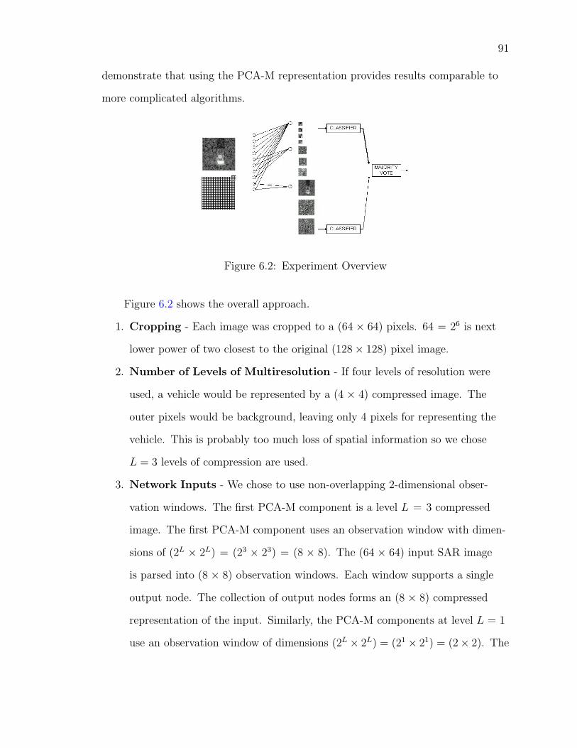
91
demonstrate that using the PCA-M representation provides results comparable to
more complicated algorithms.
Figure 6.2: Experiment Overview
Figure 6.2 shows the overall approach.
1. Cropping - Each image was cropped to a (64 × 64) pixels. 64 = 26 is next
lower power of two closest to the original (128× 128) pixel image.
2. Number of Levels of Multiresolution - If four levels of resolution were
used, a vehicle would be represented by a (4 × 4) compressed image. The
outer pixels would be background, leaving only 4 pixels for representing the
vehicle. This is probably too much loss of spatial information so we chose
L = 3 levels of compression are used.
3. Network Inputs - We chose to use non-overlapping 2-dimensional obser-
vation windows. The first PCA-M component is a level L = 3 compressed
image. The first PCA-M component uses an observation window with dimen-
sions of (2L × 2L) = (23 × 23) = (8 × 8). The (64 × 64) input SAR image
is parsed into (8 × 8) observation windows. Each window supports a single
output node. The collection of output nodes forms an (8 × 8) compressed
representation of the input. Similarly, the PCA-M components at level L = 1
use an observation window of dimensions (2L × 2L) = (21 × 21) = (2× 2). The

92
collection of (2× 2) windows support 1024 = (32× 32) outputs which form a
(32× 32) compressed representation of the input SAR image.
4. Network Structure - The overall network is a parallel structure of individ-
ual classifiers. Each individual classifier operates on a single component of
the input image. The structure of each individual classifier can be described
as One-Class-in-One-Network (OCON) (Kung, 1993, pp. 32-36). Since there
are three target classes, there are three outputs corresponding to projections
against templates for each class. The output with the highest projection
corresponds to the classification of the image based on the given compo-
nent. The final classification is based on a majority vote among individual
classifiers.
5. Network Weights - The network weights (templates) are the normalized
averages for the appropriate components of images in training set. Con-
sider the individual classifier corresponding to the first component (highest
compression, highest energy). The weights of the connections to the out-
put corresponding to the BMP-2 class are obtained by averaging the first
components of BMP-2 images.
6. Overall Classification - The final classification can be based on a majority
vote among individual classifiers. Although correlations are known to be
useful between components (Penev and Atick, 1996), and more elaborate
committee classifier structures are possible (Hu et al., 1997), a majority vote
classifier was sufficient for this experiment. A minimum number of votes can
be used to set a threshold for rejecting an image (detection). Alternatively,
the outputs of the parallel networks can be summed so that classification and
rejection are done only at this final stage.

93
6.3 Basis Arrays for PCA-M
An input image must be decomposed before processing the components
of an image. Like standard PCA, the basis for PCA-M is based on eigenvalue
decomposition of a signal’s autocorrelation matrix. Much of the mathematical
groundwork and many of the algorithms that are used for PCA are applicable to
PCA-M with minor modification and were discussed in chapter 4. Each SAR image
was decomposed using multiresolution PCA with L = 3 levels of multiresolution.
Figure 6.3: Three Levels of Decomposition on the Approximation
The PCA-M basis functions shown in Figure 6.3. Resolution decreases from top-to-
bottom, and energy decreases from left-to-right. The basis shown in the top row of
figure 6.3 are (8 × 8) arrays (top row), the middle row contains (4× 4) arrays, and
the bottom row contains (2× 2) arrays.
We use the term “basis” in the context of an overcomplete basis. Orthogo-
nality and ordering by energy holds only for arrays within a given resolution. The
highest level basis, level 3 in this application, is conventional PCA. The lowest
component level (level 1) is also conventional PCA because of the low degree
of freedom relative to the constraints imposed by PCA-M. A separable (2 × 2)

94
PCA decomposition of a Toeplitz autocorrelation matrix is constrained to be an
odd-even decomposition.
The actual PCA-M decomposition is done with a linear network. The com-
ponents are ordered by output node. The ordering is significant because of the
dependence of an output on prior outputs. The overall strategy produces outputs
that are of non-decreasing resolution and of decreasing energy (except when the
resolution changes).
6.3.1 Level 3 Components
The first four components are level 3 components. Each (64 × 64) pixel input
image is partitioned into (8×8) non-overlapping blocks. Each block contains (8×8)
pixels. Each block is multiplied against the top-left basis function in Figure 6.3.
The products form an (8× 8) image that is the first component of the input image.
The procedure is repeated for components 2 − 4. Level 3 components have the
lowest spatial resolution since each pixel of these components represent a linear
combination of an 8 pixel region of the input image.
6.3.2 Level 2 Components
Each (64× 64) pixel input is partitioned into (16× 16) non-overlapping blocks.
Each block contains (4 × 4) pixels. Each block is multiplied and projected against
the middle-left basis function in Figure 6.3. The products form an (16× 16) image
that is the fifth component of the input image. The procedure is repeated for
components 6 and 7.
6.3.3 Level 1 Components
Each (64× 64) pixel input is partitioned into (32× 32) non-overlapping blocks.
Each block contains (2 × 2) pixels. Each block is multiplied and projected against
the bottom-left basis function in Figure 6.3. The products form an (32× 32) image
that is the eighth component of the input image. The procedure is repeated for

95
components 9 and 10. Level 1 components have the highest spatial resolution since
each pixel of these components represent a linear combination of an (2) pixel region
of the input image.
6.3.4 Decorrelation between Levels
It is possible to decrease the correlation between components at different
levels by deflating the input before calculating components at a lower level. For
example, reconstruct an estimate of the original image from the level 3 components.
Subtract the estimate from the original input and use the deflated image for
constructing level 2 components. This step would not be needed if the basis
functions were orthogonal between levels. However, explicitly deflate the input
image degraded classifier performance.
A sample decomposition (middle) and a close-up of the first component
(right) are shown in Figure 6.4. The middle display shows item four level three
components which correspond to the approximation and 3 detail images of a
differential image pyramid. The three level two (16 × 16) components, and three
level one (32 × 32) components correspond to detail images. The number of
components at each level is motivated only for comparison with approximation and
detail signals in wavelet multiresolution analysis. The number of levels was based
on performance in other applications.
Figure 6.4: PCA-M Decomposition of a BMP2 Input

96
6.4 A Component Classifier
Classification is actually performed by several independent classifiers working
in parallel. In this section we will step through the portion of the network that
uses the first component of each input image for classification. The first PCA-
M component has the highest energy PCA and the coarsest spatial resolution,
Interpreting the basis function as an eigenfilter, this component has the largest
number of taps that leads to the highest spatial frequency resolution.
Figure 6.5: The Templates for Three Classes for PCA-M Component 1
There are N = 128 SAR images. Denote the first component of each image by
{x1n}, with n = [1, 2, ..., N ].
Double subscripts are not needed since only one component is under consideration.
There are K = 3 classes,
{Ck}, with k = [1, 2, K].
The class templates are the normalized averages over the training set components
for each class. Denote the (8× 8) templates (Figure 6.5) by
{m1k}, with k = [1, 2, K].
For each (8× 8) input x1, take the scalar product,
yk =8
∑
r=1
8∑
c=1
{x1}(r,c) × {m1k}(r,c).

97
Construct the K-component vector,
y1 = [y1y2y3]T .
Each original (64× 64) image x has been linearly mapped to an (8× 8) component
x1, that in turn was mapped to a (3× 1) vector y1.
{x}(64×64) 7→ {x1}(8×8) 7→ {y1}(3×1)
The classifier assignment rule is
x 7→ Ck, k ∈ K , if yk = max∀j∈K
{yj(x1,m1k)}. (6.1)
The experimental results are presented in Table 6.2. All the training images were
correctly classified except for one BTR-70 that was misclassified as a T-72. Seven
of the test target images were misclassified. Without thresholds, all the non-target
vehicles (confusers) were classified as BTR-70’s.
Table 6.2: Classification using First Component
First Component BMP-2 T-72 BTR-70 TOTAL
BMP-2 TRAIN 20 0 0 20
BMP-2 TEST 24 1 0 25
T-72 TRAIN 0 20 0 20
T-72 TEST 5 20 0 25
BTR-70 TRAIN 0 1 19 20
BTR-70 TEST 0 1 17 18
CONFUSER 0 0 40 40
Figure 6.6 shows how the (64× 64) images x were projected onto the 3-vectors
y1 using only the first component. The images of target vehicles are expected to
cluster along one of the axis and away from the origin.

98
Figure 6.6: First Component of SAR Images Projected to 3-Space
Even with just one component, misclassification is only 7/68 = 10.3% in the
test set, and 1/68 = 1.5% in the training set. We will later implement detection
by using minimum thresholds, tk, for each class. However, we will first consider
classification using more than one component.
6.5 Classifications using Several Components
Classification using any other single component is identical to the procedure
outlined for the first component. Figure 6.7 shows the templates for other PCA-M
Components.
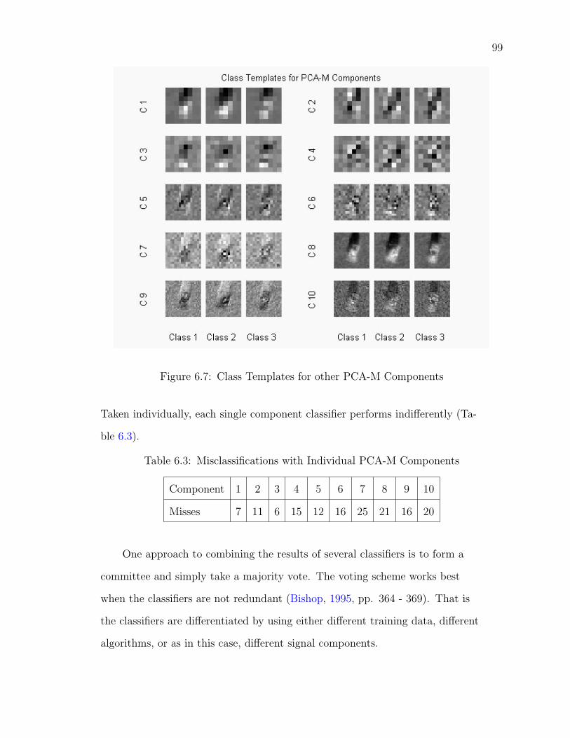
99
Figure 6.7: Class Templates for other PCA-M Components
Taken individually, each single component classifier performs indifferently (Ta-
ble 6.3).
Table 6.3: Misclassifications with Individual PCA-M Components
Component 1 2 3 4 5 6 7 8 9 10
Misses 7 11 6 15 12 16 25 21 16 20
One approach to combining the results of several classifiers is to form a
committee and simply take a majority vote. The voting scheme works best
when the classifiers are not redundant (Bishop, 1995, pp. 364 - 369). That is
the classifiers are differentiated by using either different training data, different
algorithms, or as in this case, different signal components.

100
Our approach was to add the outputs of each classifier. Denoting the number
of components by M = 10, and the 3-vectors corresponding to component m by
ym,
Y =∑
m∈M
ym
Indexing the input images, an image xn is represented by a 3-vector Yn that is
the sum of the 3-vectors corresponding to each component of that image. Each
component of Yn represents some likelihood that image xn belongs to one of the
target classes.
For convenience, each 3-vector Y is scaled so that the components sum to one,
then translated so that [1/31/31/3] (completely ambiguous with equal projections
against each class) is at the origin. Tables 6.4 and 6.5 show that the component
classifications can be combined constructively.
Table 6.4: Error Rate (5/68 = 7.4%) using 3 Components
3 Components BMP-2 T-72 BTR-70 TOTAL
TRAIN 0/20 0/20 0/20 0/60
TEST 0/25 4/25 1/18 5/68
TOTAL 0/45 4/45 1/38 5/128
Table 6.5: Error Rate (2/68 = 3.0%) using 10 Components
10 Components BMP-2 T-72 BTR-70 TOTAL
TRAIN 0/20 0/20 0/20 0/60
TEST 1/25 1/25 0/18 2/68
TOTAL 1/45 1/45 0/38 2/128
Each PCA-M component represents a projection of an image into a lower dimen-
sion subspace. While two classes may overlap at a single projection, two classes

101
should not resemble each other across all projections. Figure 6.8 shows how using
all components mapped the images xn into 3-vectors Yn. The clusters for training
and test data are separated probably from the differences in depression angle.
Figure 6.8: Clustering in 3-Space using All PCA-M Components
It appears that the 0◦ − 30◦ sector is easy to classify. While the results in this
sector are excellent, the overall unconditional Pcc is about 89% and close to the
baseline template matching results (Velten et al., 1998). The overall results for
all aspect angles (0◦ − 360◦) are shown in Table 6.6 for template matching and
Table 6.7 for PCA-M. Better results were obtained using support vector and
information-theoretic approaches (Zhao et al., 2000).

102
Table 6.6: Overall Unconditional Pcc with Template Matching
BMP-2 T-72 BTR-70
BMP-2 87.7% 1.6% 10.7%
T-72 8.8% 87.9% 3.3%
BTR-70 2.1% 0.0% 97.9%
Table 6.7: Overall Unconditional Pcc with PCA-M
BMP-2 T-72 BTR-70
BMP-2 91.0% 5.4% 3.6%
T-72 12.4% 82.9% 4.7%
BTR-70 0.5% 0.0% 99.5%
6.6 A Simple Discriminator
Discrimination should probably be performed by a separate network. Only
the inputs that are identified as targets would be evaluated by the classifier.
From Figure 6.8, it is observed that all the classes form clusters that are convex
and almost non-overlapping. Further, each axis of Figure 6.8 corresponds to a
probability of belonging to a class. The classifier of the preceding section provides
information that useful for evaluating the probability of belonging to each class. An
independent threshold is established for each axis. An input is rejected if it falls
below a threshold value for all three axes (target classes). Otherwise, it is treated
as a classification problem.
The classifier assignment rule (Equation 6.1) is
x 7→ Ck, k ∈ K , if yk = max∀j∈K
{yj(x,mk)}.
When using y to classify an image, the components of y = [y1y2y3]T interact only
when the most likely class is determined from the maximum component. After

103
the most likely class is selected we can use that component for rejection. Table 6.8
summarizes the data used to select a threshold from the training data.
Table 6.8: Determining an Threshold for Detection
OUTSIDE CLASS INSIDE CLASS
AVG MAX MIN AVG
BMP-2 −0.0054 −0.0012 0.0105 0.0129
T-72 −0.0072 −0.0014 0.0086 0.0149
BTR-70 −0.0084 −0.0008 0.0040 0.0143
The first row of Table 6.8 represents statistics on just the first component of
y. The training data from classes 2 and 3 have an average avg(y1)OUT = −0.0054,
and a maximum max(y1)OUT = −0.0012. The training data is centered at
avg(y1)IN = 0.0105, with a minimum min(y1)IN = 0.0129. By selecting a threshold
between max(y1)OUT = −0.0012 and min(y1)IN = 0.0129, some rejection is
performed. For each class we chose as a threshold,
tm = (avg(ym)OUT + avg(ym)IN)/2 (6.2)
We modify the assignment rule,
x 7→ Ck, k ∈ K , if yk = max∀j∈K
{yj(x,mk)}, and yk > tk. (6.3)
Better rejection performance will not be obtained without more data. Clas-
sifier performance using all ten components and the outlined rejection scheme is
summarized in Tables 6.9 and 6.10.

104
Table 6.9: Ten Components without Rejection
All Component BMP-2 T-72 BTR-70 TOTAL
BMP-2 TRAIN 20 0 0 20
BMP-2 TEST 24 1 0 25
T-72 TRAIN 0 20 0 20
T-72 TEST 1 24 0 25
BTR-70 TRAIN 0 0 20 20
BTR-70 TEST 0 0 18 18
CONFUSER 24 4 12 40
Table 6.10: Ten Components with Rejection
All Components BMP-2 T-72 BTR-70 REJECT TOTAL
BMP-2 TRAIN 20 0 0 0 20
BMP-2 TEST 22 1 0 2 25
T-72 TRAIN 0 20 0 0 20
T-72 TEST 0 18 0 7 25
BTR-70 TRAIN 0 0 20 0 20
BTR-70 TEST 0 0 17 1 18
CONFUSER 0 0 2 38 40
Misclassification is 1/68 = 1.47% with a Pfa of 2/40 = 5.00% and a Pd of
1− (10/68) = 85.29%. Some adjustment of rejection during operation yields better
results.
6.7 False-Positive and False-Negative Errors
This section examines the performance of the system over a range of threshold
values. Specifically we wish to determine the misclassifications and Pfa when
Pd = 90%. The methodology follows (refer to Table 6.11):

105
1. The initial thresholds were determined by minimum values needed to cor-
rectly classify the training data; the values are shown in the first column. We
noted that using these thresholds gave good rejection (95%) of the confusers
(Table 6.10), but also rejected a lot of the test data. Conceptualize this step
as constructing a tight cube about the training data.
2. We then look at the minimum values needed to best (best without the
constraint of rejecting confusers) classify the test data. The threshold values
appear in the second column. We note that rejection is poor (55%) here,
but that misclassification is only 3%. These values are shown in the second
column. Picture this as a larger cube that encompasses the training and test
data (as well as some confusers).
3. These values in the first two columns fix the range through that the threshold
values are varied for optimization. Each of the thresholds is independent.
This means that as we vary a cube between the tight cube and large cube,
each side can be optimized independently. Figure 6.9 shows the false-positive
versus false-negative errors as the threshold is varied.
After inspection (Figure 6.9), the values in the third column are found to be
good thresholds with about 90% rejection of test data.
The performance is shown in Table 6.12.
Table 6.11: Detector Threshold
Threshold TRAIN TEST BEST
BMP-2 0.0105 0.0024 0.0033
T-72 0.0086 -0.0023 0.0023
BTR-70 0.0040 -0.0029 0.0033

106
Figure 6.9: Probability of Detection versus False Alarm Rate
Table 6.12: Performance at 90% Pd
First Component BMP-2 T-72 BTR-70 REJECT TOTAL
BMP-2 TRAIN 20 0 0 0 20
BMP-2 TEST 23 1 0 1 25
T-72 TRAIN 0 20 0 0 20
T-72 TEST 0 21 0 4 25
BTR-70 TRAIN 0 0 20 0 20
BTR-70 TEST 0 0 17 1 18
CONFUSER 0 1 1 38 40
6.8 Observations
The SAR experiment had several interesting results. Using all components
has not been optimal; that is, there are some components that only add noise. The
performance of the classifier can be improved by selecting some optimal subset of
components. While it was disappointing that the high energy components did not
necessarily provide the best discrimination, it was not unexpected. PCA-M uses
all the information, not just the strong reflections. It was pleasant to find that this
information was useful for discrimination. PCA-M is a multiresolution technique,
but it cannot increase the input resolution. Given a low resolution representation
of a vehicle, it was questionable whether further reductions in resolution would

107
lose the spatial details for discrimination. Table 6.3 showed that the coarse spatial
resolution components contributed to discrimination. Finally, the three target class
structure of the experiment made a graphic interpretation feasible. PCA-M can be
seen to be useful for preprocessing since the each class of exemplars were clustered
into separated convex regions.

CHAPTER 7CONCLUSIONS AND FURTHER WORK
7.1 Conclusions
Given a class of images, PCA is a representation technique which selects
functions that are orthogonal, have uncorrelated projections, and are optimal for
minimizing mean square reconstruction error. Unfortunately, the computational
complexity of an analytic approach to PCA is O(N2). Finding eigencomponents
using adaptive techniques is also difficult because accurate convergence for a
component is dependent on the accuracy of other components. For example,
with deflation techniques, eigencomponents are found sequentially. As each
eigencomponent is calculated, its projection is removed from the input. Errors
in the accuracy of eigencomponents calculated early in the sequence propagate
through the deflated inputs to subsequent components.
With PCA-M, the simple modification of placing windows on the input layer
improves the stability of the convergence, reduces the computational complexity,
and adds several other features to PCA.
1. Assuming that the data has an interpretation as a time-series or image,
windows provide temporal or spatial localization, respectively.
2. Computations are reduced for analytic solutions. For example, if the original
input is length N , splitting the input into two local windows reduces the
computations from O(N2) to O((N2 )2).
3. PCA outputs are not only scalars which reflect global properties of the
input. PCA-M outputs are multi-scale feature spaces whose components are
dependent on localized properties.
108

109
Other than the constraint of windowed inputs, the remainder of the PCA-M
network is unchanged from PCA.
Adaptive networks that are used for PCA are easily modified for PCA-M. In
particular, a simple single-layer, O(N) adaptive algorithms such as GHA is easily
applied to PCA-M. The PCA-M learning rule is based on Hebbian learning and
is suitable for modeling locally stationary data. Identification of localized second-
order statistics can be used to segment time signals (Alonso-Betzanos et al., 1999)
and images (Fancourt and Principe, 1998). For stationary signals (or images that
are tagged as belonging to a given class), Hebb’s rule can be modified to resemble
the power method for faster convergence (Rao, 2000).
The mathematics of PCA-M is essentially the same as that for PCA, but
extended to quantify properties of components that are at different resolutions.
When Haykin (1994) presents the GHA network for PCA, he comments that a
good way to conceptualize the operation of the network to consider each output
individually. The weights to each GHA output node converge to the maximum
eigenvector of the input; however, the effective input to each output is different.
Essentially, the effective inputs to each node are derived through deflation.
PCA and PCA-M are similar except in the calculation of the effective inputs.
The effective inputs for each PCA-M output may be localized as well as deflated.
Just as PCA, the weights of each PCA-M output node converge to the maximum
eigenvector of its effective input. We presented the constraints to have PCA-M
operate as a PCA network, as well as the constraints to have PCA-M produce
classical (nested, orthogonal, locally supported) multiresolution components.
For pattern recognition, an optimal set of features would enhance discrim-
inability between classes and de-emphasize within-class variation. Both PCA and
multiresolution analysis have components with nice properties, but neither PCA
nor multiresolution components are selected for discriminability between classes.

110
PCA components are useful because they are the global components that are opti-
mal for characterizing a class. However, distinct classes may be well characterized
by some of the same components. Components that are good for characterization
are not necessarily optimal for discriminability. Another shortcoming of PCA
for classification is that local features are not isolated, only global features are
available.
If a feature extractor is presented with multiscale representations, extracting
multiscale features should be enhanced. If a feature extractor is presented with
localized inputs, it is easier to extract features for the localized duration or region.
Thus, while PCA-M is not by itself an optimal feature extractor, PCA-M can
enhance feature extraction by providing a representation with localized (as well as
global) multiscale components. With an appropriate representation, the complexity
of feature extraction can be reduced. We presented an experiment using PCA-M
as a pre-processor to a “linear” classifier (a classifier suitable only for linearly
separable data). On a standardized face database, our system outperformed all
other published approaches. The other classifiers are significantly more complex
than PCA-M (e.g., HMM, convolutional network, and eigenfaces).
PCA-M provides a representation which is localized, multiscale, and adapted
to the second-order statistics of a class. Without appropriate constraints, PCA-M
may not produce components which are orthogonal, or components for a nested
series of scaled subspaces. However, properties such as orthogonality and nesting
do not usually enhance feature extraction. We feel that PCA-M captures the
properties of PCA and multiresolution that are salient for feature extraction.
Multiscale representations are achieved by using representations which lose
resolution; that is, fine resolution in the input space is sacrificed. PCA-M (or
any other multiscale representation) might be improved by first increasing the
111
input resolution before the multiscale analysis. PCA-M in conjunction with a
super-resolution technique (Candocia, 1998) should improve feature extraction.
7.2 Future Work
In our implementation of PCA-M, the segmentation of the image, and the
choice of scales and number of feature space at each scale were not optimally
selected. We feel that there are several areas that could be investigated further.
7.2.1 Segmentation of the Input
Localization based on a regular partitioning of the input image is expedient
but not optimal. Pentland et al. (1994) showed that classification benefits from a
judicious selection of localized features. Local Feature Analysis (Penev and Atick,
1996) provided a statistically grounded method to automatically select localized
features. Some of the features selected by LFA corresponded to physical features
selected by Pentland et al. (1994). In the context of using PCA, Fancourt and
Principe (1998) used competitive PCA to segment textures within images. We
feel that results from other research suggest that it would be fruitful to further
investigate the segmentation of inputs and localization of features.
7.2.2 Component Selection
It seems that in the original eigenface experiment (Penev and Atick, 1996),
and in the application of the eigenfaces against the ORL database (Samaria,
1994; Giles et al., 1997), the eigenfaces were selected such that the corresponding
eigenvalues were in decreasing order. For example, when Giles et al. (1997) stated
that classification error was 10.5% with 40 eigenfaces, the implication is that he
used the 40 eigenfaces with the largest corresponding eigenvalues. However, in
our experiments, we found that selection of feature spaces based on eigenvalue
was not optimal. In our experiments, it was not possible to predict (e.g., using

112
corresponding eigenvalues or error rates against the training exemplars) whether a
feature space would improve or degrade classification.
It would be nice to have an algorithm to select and reject PCA-M components
based on classification performance. Realistically, it seems feasible to generate
an overcomplete set of PCA-M components and use feedback (training exemplar
error) to weight the feature spaces and prune some of the regions of the PCA-M
components.
7.2.3 Conditioned Data and Non-Linear Classifier
While not specific to PCA-M, classification error could be reduced by con-
ditioning the data to reduce distortion form illumination, rotation, scaling, or
translation. Distortion can be reduced through tight control of conditions during
data collection (Penev and Atick, 1996). Alternatively, distortions can be corrected
by offline processing, For example, the SAR images could be centered using a
correlator, rotationally aligned using a pose estimator (Xu et al., 1998), and closely
cropped to reduce background.
Classification can also be improved by using a classifier that is not limited
to linearly separable classes. For example, the support vector network (Burges,
1998) used in (Principe et al., 1998) against SAR data. However, the ORL and the
(0 − 30◦ sector) MSTAR images had training exemplars were linearly separated.
It seems that if the training exemplars are well clustered in feature space but
don’t generalize well, the underlying problem is in collecting exemplars that are
representative of the class.
APPENDIX AABBREVIATIONS
ACON All-Class One-Network
APEX Adaptive Principal Component Extraction
ATR Automated Target Recognition
CN Convolutional Network
DBNN Decision-Based Neural Network
DCT Discrete Cosine Transform
DFT Discrete Fourier Transform
FFT Fast Fourier Transform
FWT Fast Wavelet Transform
GHA Generalized Hebbian Algorithm
HMM Hidden Markov Model
HTK Hidden Markov Model Toolkit
KLT Karhunen-Loeve Transform
LBF Linear Basis Function
LFA Local Feature Analysis
MAXNET Maximum Discriminant Network
MLP Multilayer Perceptron
MSE Mean Squared Error
OCON One-Class One-Network
OCR Optical Character Recognition
ORL Olivetti Research Lab
PCA Principal Component Analysis
113

114
PCA-M Principal Component Analysis with Multiresolution
RBF Radial Basis Function
SAR Synthetic Aperture Radar
SNR Signal to Noise Ratio
SOFM Self-Organized Feature Map
SOM Self-Organized (Feature) Map
STFT Short-Time Fourier Transform
SVD Singular Value Decomposition
WSS Wide-sense Stationary

APPENDIX BOLIVETTI RESEARCH LABORATORY FACE DATABASE
Figure B.1: Olivetti Research Laboratory Face Database
115

APPENDIX CMSTAR IMAGES
Figure C.1: BMP2 Training and Test Data
116

117
Figure C.2: T72 Training and Test Data

118
Figure C.3: BTR70 Training and Test Data

119
Figure C.4: Confuser Data

REFERENCES
Alonso-Betzanos, A., Fontenla-Romero, O., Guijarro-Berdinas, B., and Principe,J. (1999). A multi-resolution principal component analysis neural network forthe detection of fetal heart rate patterns. 7th European Conference on IntelligentTechniques and Soft Computing, pages 1–6.
Bartlett, M. S., Lades, H. M., and Sejnowski, T. (1998). Independent componentrepresentations for face recognition. Proceedings of the SPIE Symposium onElectronic Imaging: Sciencs and Technology; Conference on Human Vision andElectronic Imaging III, 3299:528–539.
Baum, L. E. (1972). An inequality and associated maximization technique instatistical estimation for probabilistic functions of Markov processes. Inequalities,III:1–8.
Belhumeur, P. N., Hespanha, J. P., and Kriegman, D. (1997). Eigenfaces vs.fisherfaces: Recognition using class specific linear projection. IEEE Transactionson Pattern Analysis and Machine Intelligence, 19(7):711–720.
Bischof, H. (1995). Pyramidal Neural Networks. Lawrence Erlbaum Associates,Mahwah, NJ.
Bishop, C. M. (1995). Neural Networks for Pattern Recognition. Clarendon Press,Oxford.
Brennan, V. and Principe, J. (1998). Face classification using PCA and multires-olution. Proceedings IEEE Workshop on Neural Networks in Signal Processing,pages 506–515.
Brennan, V. and Principe, J. (2000). Multiresolution using principal componentanalysis. IEEE International Conference on Acoustics, Speech and SignalProcessing - Proceedings, 6:3474–3477.
Brunelli, R. and Poggio, T. (1993). Face recognition features versus templates.IEEE Transactions on Pattern Analysis and Machine Intelligence, 15(10):1042–1052.
Burges, C. J. (1998). A tutorial on support vector machines for pattern recognition.Data Mining and Knowledge Discovery, 2(2):955–974.
Candocia, F. (1998). A Unified Super-Resolution Approach for Optical andSynthetic Aperture Radar Images. PhD thesis, University of Florida.
120

121
Chellappa, R., Wilson, C., and Sirohey, S. (1995). Human and machine recognitionof faces: A survey. Proceedings of the IEEE, 83(5).
Duda, R. and Hart, P. (1973). Pattern classification and Scene Analysis. Wiley,New York, NY.
Fancourt, C. and Principe, J. (1998). Competitive principal component analysisfor locally stationary time series. IEEE Transactions on Signal Processing,46(11):3068–3081.
Fukunaga, K. (1990). Introduction to Statistical Pattern Recognition. AcademicPress, New York, NY.
Giles, C. L., Lawrence, S., Tsoi, A. C., and Back, A. (1997). Face recognition: Aconvolutional neural-network approach. IEEE Transactions on Neural Networks,8(1):98–113.
Golub, G. and Loan, C. V. (1989). Matrix Computations. Johns Hopkins UniversityPress, Baltimore, MD.
Haykin, S. (1994). Neural Networks, A Comprehensive Foundation. McMillanPublishing Company, Englewood Cliffs, NJ.
Haykin, S. (1996). Adaptive Signal Processing. Prentice-Hall, Upper Saddle River,NJ.
Hotelling, H. (1933). Analysis of a complex of statistical variables into principalcomponents. Journal Educ. Psychology, 24:417–441.
Hu, Y. H., Park, J.-M., and Knoblock, T. (1997). Committee pattern classifiers.Proceedings IEEE Int. Conf. on Acoustics, Speech, and Signal Processing,ICASSP, 4:3389–3392.
Jain, A. K. (1989). Fundamentals of Digital Image Processing. Prentice-Hall,Englewood Cliffs, NJ.
Kailath, T. (1980). Linear Systems. Prentice-Hall, Inc., Englewood Cliffs, NJ.
Kaiser, G. (1994). A Friendly Guide to Wavelets. Birkhauser, Inc., Boston, MA.
Kirby, M. and Sirovich, L. (1987). Low-dimensional procedure for the characteriza-tion of human faces. Journal of the Optical Society of America A, 4(3):519–524.
Kohonen, T. (1995). Self Organizing Maps. Springer-Verlag, Berlin, GE.
Kung, S.-Y. (1993). Digital Neural Networks. PTR Prentice Hall, Englewood Cliffs,NJ.
122
Le Cun, Y. and Bengio, Y. (1995). Convolutional networks for images, speech, andtime series. In Arbib, M. A., editor, The Handbook of Brain Theory and NeuralNetworks, pages 255–258. MIT Press, Cambridge, MA.
Oja, E. (1982). A simplified neuron model as a principal component analyzer.Journal of Mathematical Biology, 15:267–273.
Penev, P. S. (1999). Dimensionality reduction by sparsification in a local-featuresrepresentation of human faces. Unpublished, NEC Research Institute, Princeton,NJ.
Penev, P. S. and Atick, J. J. (1996). Local feature analysis: A general statisticaltheory for object representation. Network: Computation in Neural Systems,7(3):477–500.
Pentland, A., Moghaddam, B., and Starner, T. (1994). View-based and modulareigenspaces for face recognition. Proceedings of the IEEE Computer SocietyConference on Computer Vision and Pattern Recognition, pages 84–91.
Porat, B. (1994). Digital Processing of Random Signals. Prentice-Hall, Inc.,Englewood Cliffs, NJ.
Principe, J., Zhao, Q., and Xu, D. (1998). A novel ATR classifier exploiting poseinformation. Proceedings of Image Understanding Workshop, pages 833–836.
Rabiner, L. R. (1989). A tutorial on hidden markov models and selected applica-tions in speech recognition. Proceedings of of the IEEE, 77(2):257–286.
Rao, Y. (2000). Algorithms for eigendecomposition and time series segmentation.Master’s thesis, University of Florida.
Samaria, F. S. (1994). Face Recognition using Hidden Markov Models. PhD thesis,Trinity College, University of Cambridge.
Sanger, T. D. (1989). Optimal unsupervised learning in a single layer feedforwardnetwork. Neural Networks, 12:459–473.
Strang, G. and Nguyen, T. (1996). Wavelets and Filter Banks. Wellesley-CambridgePress, Wellesley, MA.
Therrien, C. (1992). Discrete Random Signals and Statistical Signal Processing.Prentice-Hall, Inc., Englewood Cliffs, NJ.
Turk, M. A. and Pentland, A. P. (1991a). Eigenfaces for recognition. Journal ofCognitive Neuroscience, 3:71–86.
Turk, M. A. and Pentland, A. P. (1991b). Face recognition using eigenfaces.Proceedings of the 1991 IEEE Computer Society Conference on Computer Visionand Pattern Recognition, 91:586–591.

123
Vapnik, V. N. (1998). Statistical Learning Theory. Wiley, New York, NY.
Velten, V., Ross, T., Mossing, J., Worrell, S., and Bryant, M. (1998). StandardSAR ATR evaluation experiments using the MSTAR public release data set.Technical report, ASC-98-0101, AFRL/SNAT, Wright-Patterson AFB.
Vetterli, M. and Kovacevic, J. (1995). Wavelets and Sub-band Coding. Prentice-Hall, Inc., Englewood Cliffs, NJ.
Xu, D., Fisher, J., and Principe, J. (1998). Mutual information approach to poseestimation. Algorithms for Synthetic Aperture Radar Imagery V, Proceedings ofthe SPIE, 3370:219–229.
Young, S. (1993). The HTK hidden markov model toolkit: Design and philosophy.Technical report, TR.153, Department of Engineering, Cambridge University.
Zhao, Q., Principe, J., Brennan, V., Xu, D., and Wang, Z. (2000). Syntheticaperture radar automatic target recognition with three strategies of learning andrepresentation. Optical Engineering, 39(5):1230–1244.

BIOGRAPHICAL SKETCH
Victor Brennan was born in Clark Air Force Base, Philippines, on November
17, 1956. He received a B.S. in chemical engineering from Carnegie-Mellon Univer-
sity in 1978, an MBA from New Mexico State University in 1983, and an MS in
electrical and computer engineering from North Carolina State University in 1987.
From 1978 to 1992, he was an officer in the U.S. Army Signal Corps. In his
last tour, Major Brennan served as Chief, Engineering and Acquisition (E&A)
Branch, US Army Mission Support Activity, Warrenton, VA. The E&A branch was
responsible for maintenance and logistical support of US Army electronic warfare
equipment worldwide.
124