Embed Size (px)
Citation preview

1
Principal component analysis(PCA) for clustering gene
expression dataKa Yee Yeung
Walter L. Ruzzo
Bioinformatics, v17 #9 (2001) pp 763-774

2
Outline of talk• Background and motivation• Design of our empirical study• Results• Summary and Conclusions

5
Principal Component Analysis(PCA)
• Reduce dimensionality• Retain as much
variation as possible• Linear transformation
of the originalvariables
• Principal components(PC’s) are uncorrelatedand ordered
PC1PC2

6
Definition of PC’s• FIRST principle component – the direction
which maximizes variability of the datawhen projected on that axis
• Second PC – the direction, among thoseorthogonal to the first, maximizingvariability
• ...• Fact: They are eigenvectors of ATA ;
eigenvalues are the variances

8
Motivation• Chu et al. [1998] identified 7 clusters using
Eisen et al.’s CLUSTER software(hierarchical centroid-link) on the yeastsporulation data set.
• Raychaudhuri et al. [2000] applied PCA tothe sporulation data, and claimed that thedata showed a unimodal distribution in thespace of the first 2 PC’s.

9
PC’s in Sporulation Data
1st two PC’s: > 90% of variance
1st three PC’s: > 95% of variance

10
“Theunimodaldistributionofexpressionin the mostinformativetwodimensionssuggeststhe genesdo not fallinto well-definedclusters.”-- Raychaudhuriet al.

11

12

15

16
PCA and clustering• Euclidean distance:
– using all p variables,Euclidean distancebetween a pair of genesunchanged after PCA[Jolliffe 1986]
– using m variables (m<p) ==>approximation
• Correlation coefficient– no general relationship
before and after PCA
PC1
18
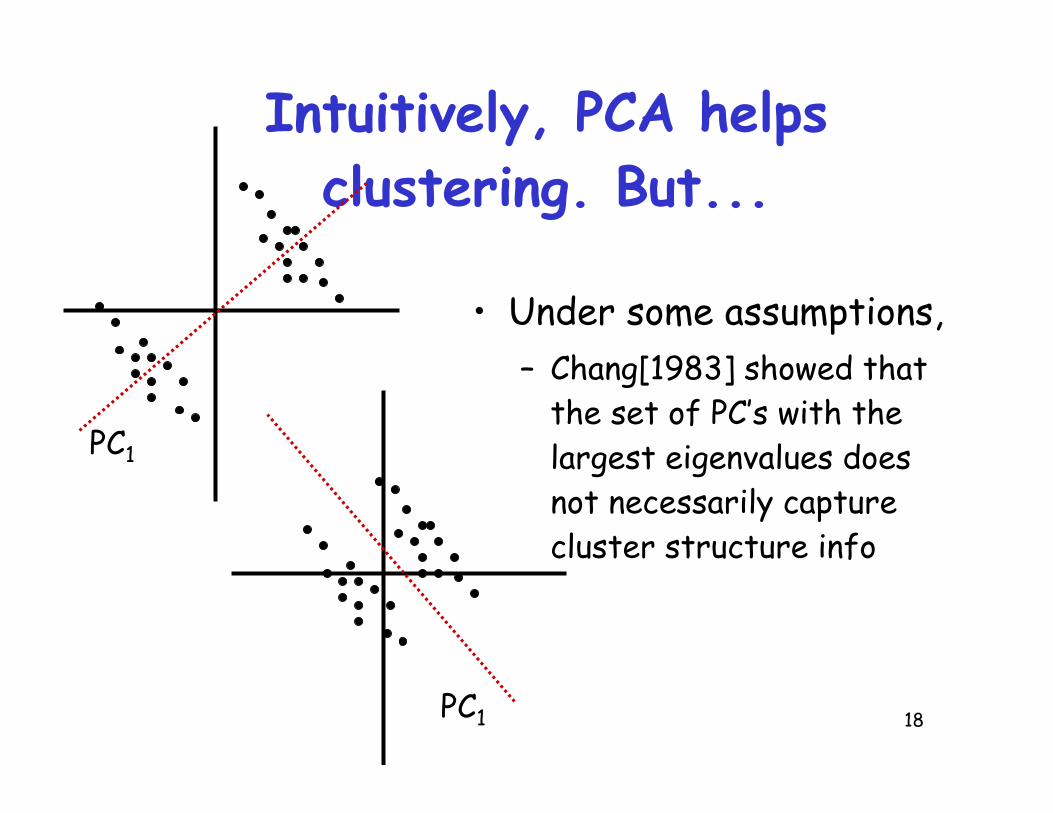
Intuitively, PCA helpsclustering. But...
• Under some assumptions,– Chang[1983] showed that
the set of PC’s with thelargest eigenvalues doesnot necessarily capturecluster structure info
PC1
PC1

19
Outline of talk• Background and motivation• Design of our empirical study• Results• Summary and Conclusions

20
Our empirical study
• Goal: Compare the clustering results withand without PCA to an external criterion:– expression data set with external criterion– synthetic data sets– methodology to compare to an external
criterion– clustering algorithms– similarity metrics

21
Ovary data (Michel Schummer)• Randomly selected cDNA’s on membrane arrays• Subset of data:
– 235 clones– 24 experiments (7 from normal tissues, 4 from
blood samples, 13 from ovarian cancers)
• 235 clones correspond to 4 genes (sizes 58,88, 57,32)
• The four genes form the 4 classes (externalcriterion)

22
PCA on ovary data• Number of PC’s to adequately represent the
data:– 14 PC’s cover 90% of the variation– scree graph
0
0.05
0.1
0.15
0.2
0.25
0.3
0.35
1 3 5 7 9 11 13 15 17 19 21 23component number
eig
en
va
lue

23
Synthetic data sets (1)• Mixture of normal distributions
– Compute the mean vector and covariance matrixfor each class in the ovary data
– Generate a random mixture of normal distributionsusing the mean vectors, covariance matrices, andsize distributions from the ovary dataHistogram of a normal class Histogram of a tumor class
freq
uenc
y
Expression level

24
Synthetic data sets (2)• Randomly permuted ovary
data– Random sample (with
replacement) theexpression levels in thesame class
– Empirical distrubutionpreserved
– But covariance matrix notpreserved
1 j p
Experimental conditions(variables)
Clon
es (o
bser
vati
ons)
1
n
class

26
Clustering algorithms andsimilarity metrics
• CAST [Ben-Dor and Yakhini 1999] with correlation– build one cluster at a time– add or remove genes from clusters based on
similarity to the genes in the current cluster
• k-means with correlation and Euclideandistance– initialized with hierarchical average-link

27
Outline of talk
• Background and motivation• Design of our empirical study• Results• Summary and Conclusions

28
PCA
Our approach
Cluster theoriginal data
Cluster with thefirst m PC’s(m=m0, …, p)
Compare toexternal criterion
Cluster with sets of PCwith “high” adjustedRand indices:– greedy approach
• exhaustive search form0 components
• greedily add the nextcomponent
– modified greedy approach
PCA
29
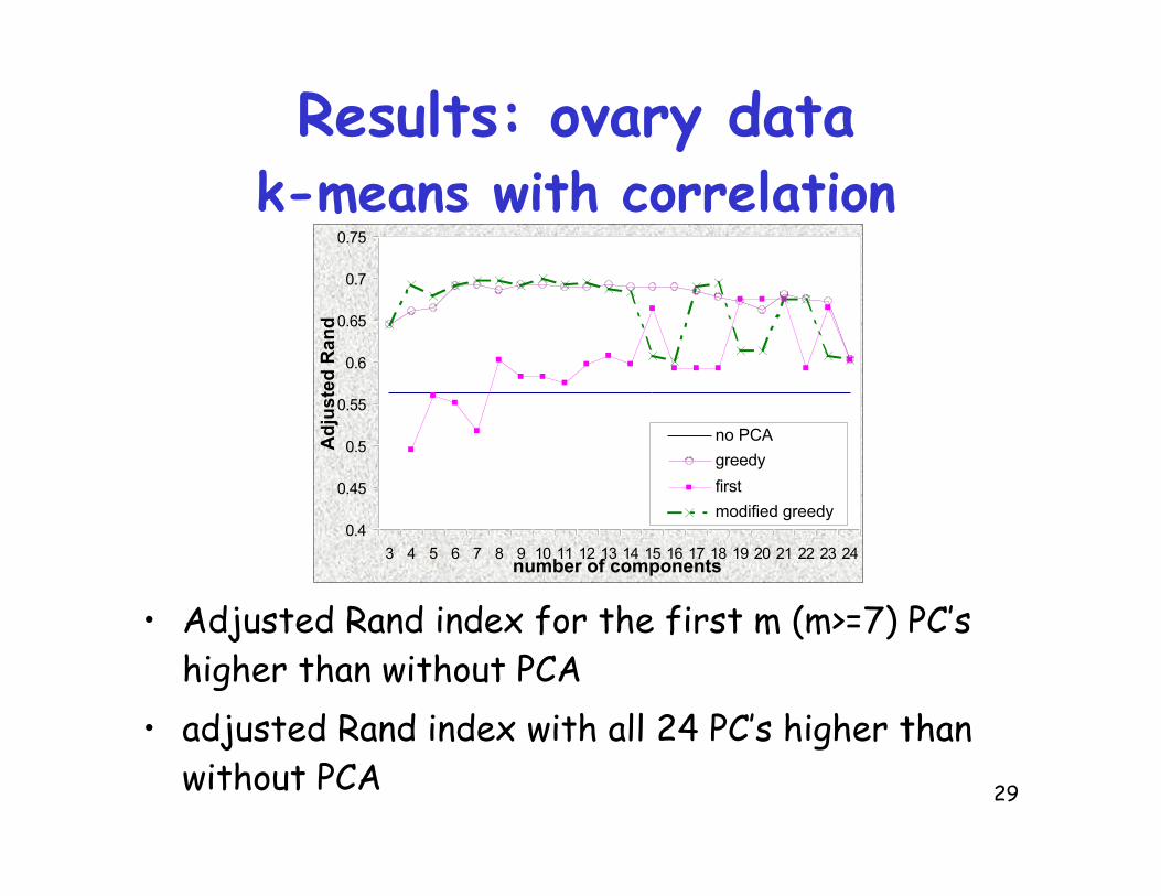
Results: ovary datak-means with correlation
• Adjusted Rand index for the first m (m>=7) PC’shigher than without PCA
• adjusted Rand index with all 24 PC’s higher thanwithout PCA
0.4
0.45
0.5
0.55
0.6
0.65
0.7
0.75
3 4 5 6 7 8 9 10 11 12 13 14 15 16 17 18 19 20 21 22 23 24number of components
Ad
just
ed R
and
no PCA
greedy
first
modified greedy

30
Results: ovary datak-means with Euclidean distance
• Sharp drop of adjusted Rand index from the first3 to first 4 PC’s
0.4
0.45
0.5
0.55
0.6
0.65
0.7
0.75
2 4 6 8 10 12 14 16 18 20 22 24number of components
Ad
just
ed R
and
firstno PCAgreedymodified greedy

31
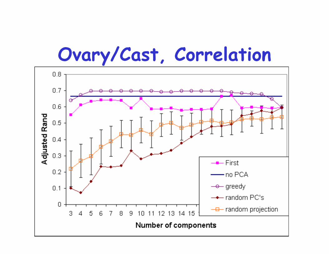
Results: ovary dataCAST with correlation
• Adjusted Rand index on the first components <=without PCA
• greedy or modified greedy approach usually achievehigher adjusted Rand than without PCA
0.4
0.45
0.5
0.55
0.6
0.65
0.7
0.75
3 4 5 6 7 8 9 10 11 12 13 14 15 16 17 18 19 20 21 22 23 24Number of components
Ad
just
ed R
and
First
no PCA
greedy
modified greedy
32
Ovary/Cast, Correlation
36
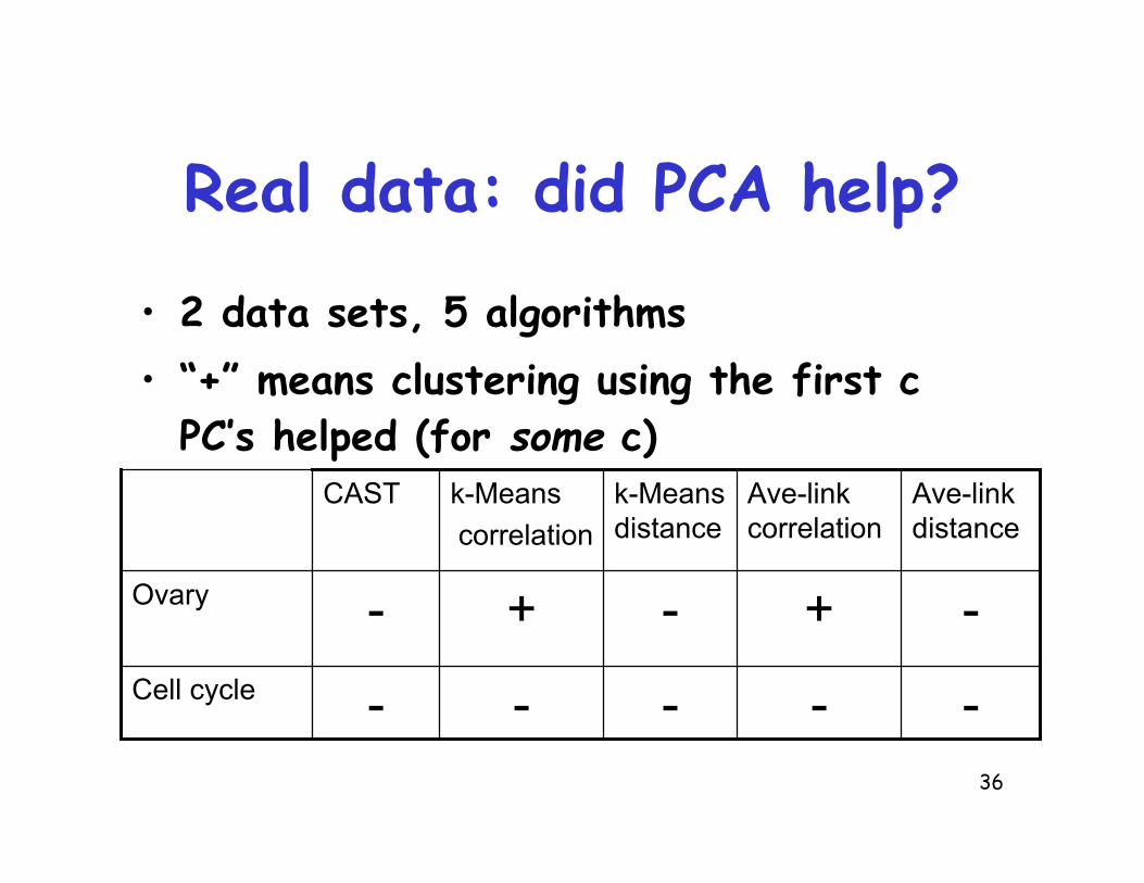
Real data: did PCA help?
• 2 data sets, 5 algorithms• “+” means clustering using the first c
PC’s helped (for some c)
-----Cell cycle
-+-+-Ovary
Ave-linkdistance
Ave-linkcorrelation
k-Meansdistance
k-Means
correlation
CAST

37
Synth data: Did PCA help?p-values from Wilcoxon signed rank test. (p<5% are bold)
Synthetic data Alternative CAST k-mean k-mean ave-link ave-link hypothesis corr. Corr dist corr dist
Mixture of normal no PCA > first 0.039 0.995 0.268 0.929 0.609Mixture of normal no PCA < first 0.969 0.031 0.760 0.080 0.418
Random resampled no PCA > first 0.243 0.909 0.824 0.955 0.684Random resampled no PCA < first 0.781 0.103 0.200 0.049 0.337
Cyclic data no PCA > first 0.023 NA 0.296 0.053 0.799Cyclic data no PCA < first 0.983 NA 0.732 0.956 0.220

38
Some successesAlter,O., Brown,P.O. and Botstein,D. (2000)Singular value decomposition for genome-wideexpression data processing and modeling. Proc.Natl Acad. Sci. USA, 97, 10 101_10 106.
Holter,N.S., Mitra,M., Maritan,A., Cieplak,M.,Banavar,J.R. and Fedoroff,N.V. (2000)Fundamental patterns underlying gene expressionprofiles: simplicity from complexity. Proc. NatlAcad. Sci. USA, 97, 8409_8414.Hastie T, Tibshirani R, Eisen MB, Alizadeh A, Levy R,Staudt L, Chan WC, Botstein D, Brown P. 'Geneshaving' as a method for identifying distinct sets ofgenes with similar expression patterns. GenomeBiol. 2000;1(2):RESEARCH0003.

39
Outline of talk
• Background and motivation• Design of our empirical study• Results• Summary and Conclusions

40
Summary & Conclusions (1)• PCA may not improve cluster quality
– first PC’s may be worse than without PCA– another set of PC’s may be better than first PC’s
• Effect of PCA depends on clusteringalgorithms and similarity metrics– CAST with correlation: first m PC’s usually worse
than without PCA– k-means with correlation: usually PCA helps– k-means with Euclidean distance: worse after the
first few PC’s

41
Summary & Conclusions (2)
• No general trends in the components chosenby the greedy or modified greedy approach– usually the first 2 components are chosen by the
exhaustive search step
• Results on the synthetic data similar to realdata

42
Bottom Line
• Successes by other groups makeit a technique worth considering,but it should not be appliedblindly.

43
Acknowledgements• Ka Yee Yeung• Michèl Schummer
More Infohttp://www.cs.washington.edu/homes/{kayee,ruzzo}
UW CSE Computational Biology Group

48
Mathematical definition of PCA• The k-th PC:
• First PC :maximizevar (z1)=a1
TSa1, such thata1
Ta1=1, where S is thecovariance matrix
• k-th PC: maximizevar (zk)=ak
TSak, such thatak
Tak=1 and akTai=0,
where i < k
1 j p
Experimental conditions(variables)
Gene
s (o
bser
vati
ons)
i Xi,j
Vector xj
1
n
j
p
jjkk xz Â
=
=1
,a
49
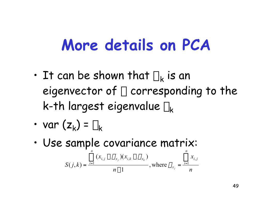
More details on PCA
• It can be shown that ak is aneigenvector of S corresponding to thek-th largest eigenvalue lk
• var (zk) = lk
• Use sample covariance matrix:
n
x
n
xxkjS
n
iji
x
n
ixkixji
j
kj ÂÂ== =
-
--= 1
,1
,,
where,1
))((),( m
mm