Clustering and Principal Component Methods - Freefactominer.free.fr/more/tutorial_2010_clustering.pdf · Clustering and Principal Component Methods ... PCA as a preprocessing

Clustering Methods Preprocessing Graphical Complementarity References

Clustering and Principal ComponentMethods

1 Clustering Methods

2 Principal Components Methods as a Preprocessing Step

3 Graphical Complementarity

1 / 24


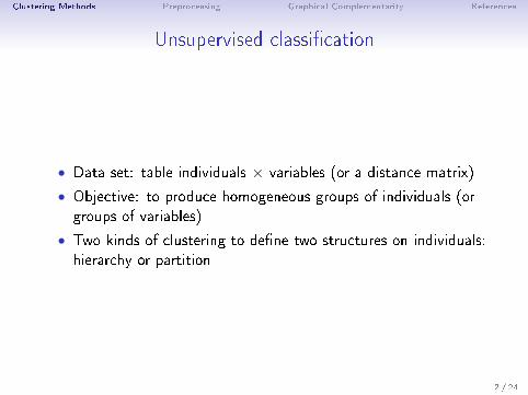
Unsupervised classi�cation

• Data set: table individuals × variables (or a distance matrix)

• Objective: to produce homogeneous groups of individuals (orgroups of variables)

• Two kinds of clustering to de�ne two structures on individuals:hierarchy or partition

2 / 24


Hierarchical Clustering

Principle: sequentially agglomerate (clusters of) individuals using

• a distance between individuals: City block, Euclidean

• an agglomerative criterion: single linkage, complete linkage,average linkage, Ward's criterion

Single linkage

Complete linkage

City-blockEuclidean

Representation with a dendrogram

⇒ Eulidean distance is used in principal component methods⇒ Ward's criterion is based on multidimensional variance (inertia)which is the core of principal component methods

3 / 24


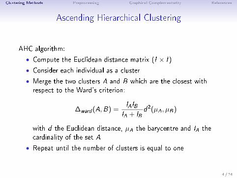
Ascending Hierarchical Clustering

AHC algorithm:

• Compute the Euclidean distance matrix (I × I )

• Consider each individual as a cluster

• Merge the two clusters A and B which are the closest withrespect to the Ward's criterion:

∆ward (A,B) =IAIB

IA + IBd2(µA, µB)

with d the Euclidean distance, µA the barycentre and IA thecardinality of the set A

• Repeat until the number of clusters is equal to one

4 / 24


Ward's criterion

• Individuals can be represented by a cloud of points in RK

• Total inertia = multidimensional variance

With Q groups of individuals, inertia can be decomposed as:

K∑k=1

Q∑q=1

Iq∑i=1

(xiqk−x̄k)2 =K∑k=1

Q∑q=1

Iq(x̄qk−x̄k)2+K∑k=1

Q∑q=1

Iq∑i=1

(xiqk−x̄qk)2

Total inertia = Between inertia + Within inertia

5 / 24


Ward's criterion

? ? ?

Step 1: 1 cluster = 1 individualWithin = 0Between = Total

Step I : only 1 clusterWithin = TotalBetween = 0

Step I-2 : 3 clusters

Step I-1 : 2 clusters to define

⇒ Ward minimizes the increasing of within inertia6 / 24


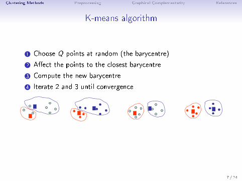
K-means algorithm

1 Choose Q points at random (the barycentre)

2 A�ect the points to the closest barycentre

3 Compute the new barycentre

4 Iterate 2 and 3 until convergence

7 / 24


PCA as a preprocessing

With continuous variables:⇒ AHC and k-means onto the raw data⇒ AHC or k-means onto principal components

PCA transforms the raw variables into orthogonal principalcomponents F.1, ...,F.K with decreasing variance λ1 ≥ λ2 ≥ ...λK

Data NoiseStructurePCA

x.1 x.Kx.k F1 FQ FK

⇒ Keeping the �rst components makes the clustering more robust⇒ But, how many components do you keep to denoise?

8 / 24


MCA as a preprocessing

Clustering on categorical variables: which distance to use?

• with two categories: Jaccard index, Dice's coe�cient, simplematch, etc. Indices well-�tted for presence/absence data

• with more than 2 categories: use for example the χ2-distance

Using the χ2-distance ⇔ computing distances from all the principalcomponents obtained from MCA

In practice, MCA is used as a preprocessing in order to

• transform categorical variables in continuous ones

• delete the last dimensions to make the clustering more robust

9 / 24


MFA as a preprocessing

i

i’

X1 X2

MFA balances the in�uence of the groups when computingdistances between individuals

d2(i , i ′) =J∑

j=1

1√λj

Kj∑k=1

(xik − xi ′k)2

AHC or k-means onto the �rst principal components (F.1, ...,F.Q)obtained from MFA allows to• take into account the groups structure in the clustering• make the clustering more robust by deleting the last dimensions

10 / 24


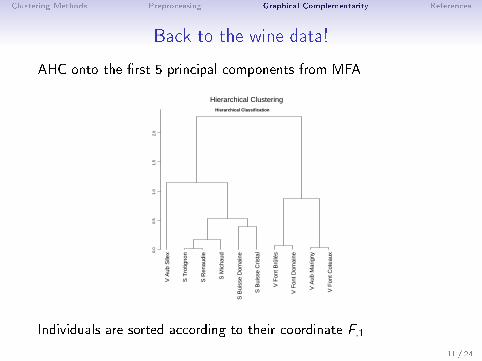
Back to the wine data!

AHC onto the �rst 5 principal components from MFA

Hierarchical Clustering

V A

ubS

ilex

S T

rotig

non

S R

enau

die

S M

icha

ud

S B

uiss

e D

omai

ne

S B

uiss

e C

rista

l

V F

ont B

rûlé

s

V F

ont D

omai

ne

V A

ubM

arig

ny

V F

ont C

otea

ux 0.

00.

51.

01.

52.

0

Hierarchical Classification

Individuals are sorted according to their coordinate F.1

11 / 24


Why sorting the tree?

X <- c(6,7,2,0,3,15,11,12)

names(X) <- X

library(cluster)

par(mfrow=c(1,2))

plot(as.dendrogram(agnes(X)))

plot(as.dendrogram(agnes(sort(X))))0

24

68

6 7 2 3 0 15 11 12

02

46

8

0 2 3 6 7 11 12 15

12 / 24


Partition from the tree

An empirical number of clusters is suggested (minqWq−Wq+1

Wq−1−Wq)

0.0

0.5

1.0

1.5

2.0Hierarchical Clustering

inertia gain V

Aub

Sile

x

S T

rotig

non

S R

enau

die

S M

icha

ud

S B

uiss

e D

omai

ne

S B

uiss

e C

rista

l

V F

ont B

rûlé

s

V F

ont D

omai

ne

V A

ubM

arig

ny

V F

ont C

otea

ux 0.

00.

51.

01.

52.

0

Hierarchical Classification

13 / 24


Hierarchical tree on the principal component map

-2 -1 0 1 2 3

0.0

0.5

1.0

1.5

2.0

2.5

-3

-2

-1

0

1

2

Dim 1 (42.52%)

Dim

2 (

24.4

2%)

heig

ht

cluster 1 cluster 2 cluster 3 cluster 4 cluster 5

V Aub Silex

S Trotignon

S Buisse Domaine

S Renaudie

S Michaud S Buisse Cristal

V Font Brûlés V Font Domaine

V Aub Marigny

V Font Coteaux

Hierarchical clustering on the factor map

-2 -1 0 1 2 3

0.0

0.5

1.0

1.5

2.0

2.5

-3

-2

-1

0

1

2

Dim 1 (42.52%)

Dim

2 (

24.4

2%)

heig

ht


V Aub Silex

S Trotignon

S Buisse Domaine

S Renaudie

S Michaud S Buisse Cristal

V Font Brûlés V Font Domaine

V Aub Marigny

V Font Coteaux

Hierarchical clustering on the factor map

Hierarchical tree gives an idea of the other dimensions

14 / 24


Partition on the principal component map

-2 -1 0 1 2 3 4

-3-2

-10

12

Dim 1 (42.52%)

Dim

2 (2

4.42

%)

V Aub Silex

S Trotignon

S Buisse Domaine

S Renaudie

S Michaud

S Buisse Cristal

V Font Brûlés

V Font Domaine

V Aub Marigny

V Font Coteaux


-2 -1 0 1 2 3 4

-3-2

-10

12

Dim 1 (42.52%)

Dim

2 (2

4.42

%)

V Aub Silex

S Trotignon

S Buisse Domaine

S Renaudie

S Michaud

S Buisse Cristal

V Font Brûlés

V Font Domaine

V Aub Marigny

V Font Coteaux


Continuous view (principal components) and discontinuous(clusters)

15 / 24


Cluster description by variables

v.test =x̄q − x̄√s2

Iq

(I−IqI−1

) ∼ N (0, 1) H0 : x̄q = x̄

with x̄q the mean of variable x in cluster q, x̄ (s) the mean(standard deviation) of the variable x in the data set, Iq thecardinal of cluster q

$desc.var$quanti$`2`

v.test Mean in Overall sd in Overall p.value

category mean category sd

O.passion_C 2.58 6.17 4.61 0.79 1.18 0.01

O.citrus 2.50 5.40 3.66 0.22 1.37 0.01

O.passion_S 2.45 5.69 4.18 0.54 1.20 0.01

....

Typicity -2.42 1.36 3.91 0.72 2.07 0.02

O.candied.fruit -2.44 0.78 2.58 0.16 1.45 0.01

O.alcohol_S -2.48 3.98 4.33 0.13 0.28 0.01

Surface.feeling -2.52 2.63 3.62 0.12 0.77 0.01

16 / 24


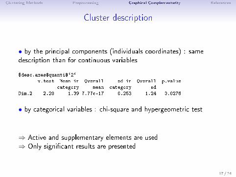
Cluster description

• by the principal components (individuals coordinates) : samedescription than for continuous variables

$desc.axes$quanti$`2`

v.test Mean in Overall sd in Overall p.value

category mean category sd

Dim.2 2.20 1.39 7.77e-17 0.253 1.24 0.0276

• by categorical variables : chi-square and hypergeometric test

⇒ Active and supplementary elements are used⇒ Only signi�cant results are presented

17 / 24


Cluster description by individuals

• parangon: the closest individuals to the barycentre of the cluster

mini∈q

d(xi ., µq) with µq the barycentre of cluster q

• speci�c individuals: the furthest individuals to the barycentres ofthe other clusters (the individuals sorted according to their distancefrom the highest to the smallest to the closest barycentre)

maxi∈q

minq′ 6=q

d(xi ., µq′)

desc.ind$para

cluster: 2

S Renaudie S Trotignon S Michaud

0.1002890 0.3101154 0.3640145

------------------------------------------

desc.ind$dist

cluster: 2

S Trotignon S Renaudie S Michaud

1.934103 1.687849 1.265386

------------------------------------------

18 / 24


Complementarity between hierarchical clustering and

partitioning

• Partitioning after AHC: the k-means algorithm is initializedfrom the barycentres of the partition obtained from the tree

• consolidate the partition• loss of the hierarchy

• AHC with many individuals: time-consuming⇒ partitioning before AHC

• compute k-means with approximately 100 clusters• AHC on the weighted barycentres obtained from the k-means⇒ top of the tree is approximately the same

19 / 24


Practice with R

res.hcpc <- HCPC(res.mfa)

##### Example of clustering on categorical data

data(tea)

res.mca <- MCA(tea,quanti.sup=19,quali.sup=20:36)

plot(res.mca,invisible=c("var","quali.sup","quanti.sup"),cex=0.7)

plot(res.mca,invisible=c("ind","quali.sup","quanti.sup"),cex=0.8)

plot(res.mca,invisible=c("quali.sup","quanti.sup"),cex=0.8)

dimdesc(res.mca)

res.mca <- MCA(tea,quanti.sup=19,quali.sup=20:36, ncp=10)

res.hcpc <- HCPC(res.mca)

20 / 24


CARME conference

International conference on Correspondence Analysis andRelated MEthods

Agrocampus Rennes (France), February 8-11, 2011

R tutorials for corresp. ana. and related methods of visualization:• S. Dray: multivariate analysis of ecological data with ade4

• O. Nenadi¢ & M. Greenacre: correspondence analysis with ca

• S. Lê: from one to multiple data tables with FactoMineR

• J. de Leeuw & P. Mair: multidimensional scaling using majorisation with smacof

Invited speakers: Monica Bécue, Cajo ter Braak, Jan de Leeuw,Stéphane Dray, Michael Friendly, Patrick Groenen, PieterKroonenberg

21 / 24


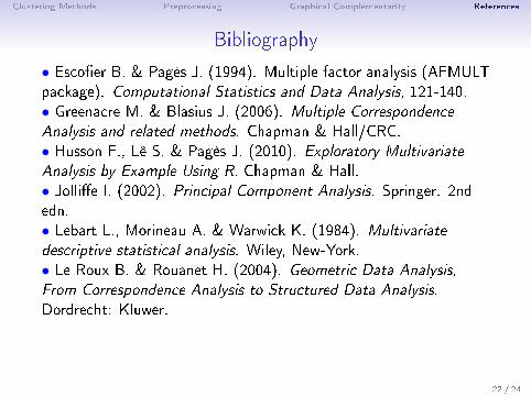
Bibliography

• Esco�er B. & Pagès J. (1994). Multiple factor analysis (AFMULTpackage). Computational Statistics and Data Analysis, 121-140.• Greenacre M. & Blasius J. (2006). Multiple Correspondence

Analysis and related methods. Chapman & Hall/CRC.• Husson F., Lê S. & Pagès J. (2010). Exploratory Multivariate

Analysis by Example Using R. Chapman & Hall.• Jolli�e I. (2002). Principal Component Analysis. Springer. 2ndedn.• Lebart L., Morineau A. & Warwick K. (1984). Multivariate

descriptive statistical analysis. Wiley, New-York.• Le Roux B. & Rouanet H. (2004). Geometric Data Analysis,

From Correspondence Analysis to Structured Data Analysis.Dordrecht: Kluwer.

22 / 24


Packages' bibliography

http://cran.r-project.org/web/views/Multivariate.html

http://cran.r-project.org/web/views/Cluster.html

• ade4 package: data analysis functions to analyse Ecological andEnvironmental data in the framework of Euclidean Exploratory methodshttp://pbil.univ-lyon1.fr/ADE-4

• ca package (Greenacre and Nenadic) deals with simple, multiple andjoint correspondence analysis• cluster package: basic and hierarchical clustering• dynGraph package: visualization software to explore interactivelygraphical outputs provided by multidimensional methodshttp://dyngraph.free.fr

• FactoMineR packagehttp://factominer.free.fr

• hopach package: builds hierarchical tree of clusters

• missMDA package: imputes missing values with multivariate data

analysis methods

23 / 24

http://cran.r-project.org/web/views/Multivariate.html

http://cran.r-project.org/web/views/Cluster.html

http://pbil.univ-lyon1.fr/ADE-4

http://dyngraph.free.fr

http://factominer.free.fr


FactoMineR

A website with documentation, examples, data sets:http://factominer.free.fr

How to install the Rcmdr menu:copy and paste the following line of code in a R session

source("http://factominer.free.fr/install-facto.r")

A book:Husson F., Lê S. & Pagès J. (2010). Exploratory Multivariate

Analysis by Example Using R. Chapman & Hall.

24 / 24

http://factominer.free.fr

Documents

Clustering and Principal Component Methods - Freefactominer.free.fr/more/tutorial_2010_clustering.pdf · Clustering and Principal Component Methods ... PCA as a preprocessing