Embed Size (px)
Citation preview

Machine Learning LabUniversity of Freiburg
Principal Component AnalysisMachine Learning Summer 2015
Dr. Joschka Boedecker
AcknowledgementSlides courtesy of Manuel Blum
Motivation
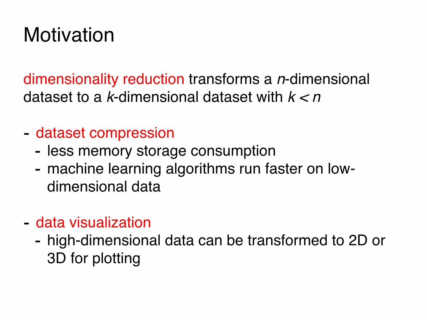
dimensionality reduction transforms a n-dimensional dataset to a k-dimensional dataset with k < n
- dataset compression- less memory storage consumption- machine learning algorithms run faster on low-
dimensional data
- data visualization - high-dimensional data can be transformed to 2D or
3D for plotting

z
Principal Component Analysis
Weight
Height
Example:
- original 2D dataset containing features weight and height
- projection on vector u
- most commonly used dimensionality reduction method- projects the data on k orthogonal bases vectors u that
minimize the projection error
u
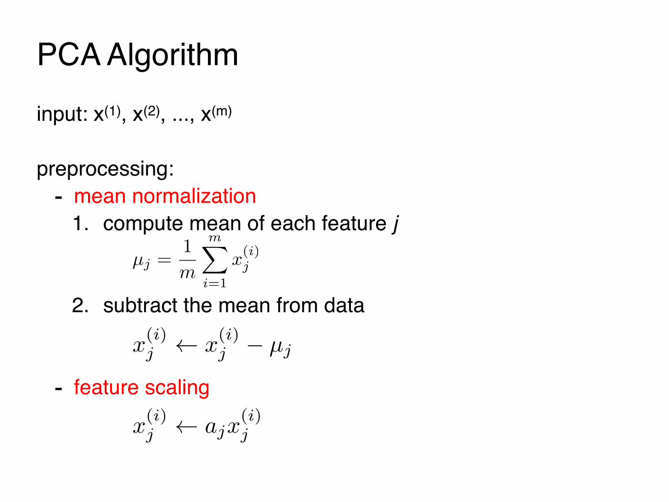
PCA Algorithminput: x(1), x(2), ..., x(m)
preprocessing:- mean normalization
1. compute mean of each feature j
2. subtract the mean from data
- feature scaling
µj =1
m
mX
i=1
x
(i)j
x
(i)j x
(i)j � µj
x
(i)j ajx
(i)j

PCA Algorithm
diagonalize covariance matrix (using SVD)S = U�1⌃U
compute covariance matrix ⌃ =1
m
mX
i=1
x
(i)x
(i)T
U is the matrix of Eigenvectors S a diagonal matrix containing the Eigenvalues
dimensionality reduction from n to k dimensions:project the data onto the Eigenvectors corresponding to the k largest Eigenvalues
z
(i) = U
Treducex
(i)

Reconstruction
z
(i) = U
Treducex
(i)
5-5 -4 -3 -2 -1 1 2 3 4
5
-5
-4
-3
-2
-1
1
2
3
4
X
Y
-6 -5 -4 -3 -2 -1 0 1 2 3 4 5 6
z_1
5-5 -4 -3 -2 -1 1 2 3 4
5
-5
-4
-3
-2
-1
1
2
3
4
X
Y
x
approx
= U
reduce
⇤ z(i)
the reconstruction of compressed data points is an approximation of the original data

Choosing kaverage squared projection error:
total variation in the data:
1
m
mX
i=1
���x(i) � x
(i)approx
���2
1
m
mX
i=1
���x(i)���2
to retain 99% of the variance, choose k to be the smallest value, such that
1m
Pm
i=1
���x(i) � x
(i)approx
���2
1m
Pm
i=1
��x
(i)��2
= 1�P
k
i=1 SiiPn
i=1 Sii
0.01
Pki=1 SiiPni=1 Sii
� 0.99

Example using Real-world Data
http://archive.ics.uci.edu/ml/
- offers 223 datasets - datasets can be used for the evaluation of ML methods- results can be compared to those of other researchers

Iris Data Set Download: Data Folder, Data Set Description
Abstract: Famous database; from Fisher, 1936
Data Set Characteristics: Multivariate Number of Instances: 150 Area: Life
Attribute Characteristics: Real Number of Attributes: 4 Date Donated 1988-07-01
Associated Tasks: Classification Missing Values? No Number of Web Hits: 348488
Source:
Creator: R.A. Fisher
Donor: Michael Marshall (MARSHALL%PLU '@' io.arc.nasa.gov)
Data Set Information:
This is perhaps the best known database to be found in the pattern recognition literature. Fisher's paper is a classic in the field and is referenced frequently to this day. (See Duda & Hart, for example.) The data set contains 3 classes of 50 instances each, where each class refers to a type of iris plant. One class is linearly separable from the other 2; the latter are NOT linearly separable from each other. Predicted attribute: class of iris plant. This is an exceedingly simple domain. This data differs from the data presented in Fishers article (identified by Steve Chadwick, spchadwick '@' espeedaz.net ). The 35th sample should be: 4.9,3.1,1.5,0.2,"Iris-setosa" where the error is in the fourth feature. The 38th sample: 4.9,3.6,1.4,0.1,"Iris-setosa" where the errors are in the second and third features.
Attribute Information:
1. sepal length in cm 2. sepal width in cm 3. petal length in cm 4. petal width in cm 5. class: Iris Setosa, Iris Versicolour, Iris Virginica

PCA on the Iris dataset
−4 −3 −2 −1 0 1 2 3−3
−2
−1
0
1
2
3
Iris SetosaIris VersicolourIris Virginica
U =
0
BB@
�0.5224 �0.3723 0.7210 0.26200.2634 �0.9256 �0.2420 �0.1241�0.5813 �0.0211 �0.1409 �0.8012�0.5656 �0.0654 �0.6338 0.5235
1
CCA
given: data matrix X
preprocessing: - mean normalization- feature scaling
compute covariance matrix:
S =
0
BB@
2.8914 0 0 00 0.9151 0 00 0 0.1464 00 0 0 0.0205
1
CCA
⌃ =1
m
mX
i=1
x
(i)x
(i)T
compute eigenvectors and eigenvalues:
reduce U to k components
z
(i) = U
Treducex
(i)

Final Remarks
- PCA assumes that most of the information is contained in the direction with the highest variance
Weight
Height
- PCA is an unsupervised method - when used as a preprocessing step for supervised learning the performance can drop significantly
- there exist nonlinear extensions (Kernel PCA)- PCA can only realize linear transformations
- PCA-transformed data is uncorrelated
- PCA is often used to reduce the noise in a signal