Principal Component Analysis of High Frequency Data∗

Yacine Aït-Sahalia†

Department of Economics

Princeton University and NBER

Dacheng Xiu‡

Booth School of Business

University of Chicago

This Version: October 7, 2016

Abstract

We develop the necessary methodology to conduct principal component analysis at high

frequency. We construct estimators of realized eigenvalues, eigenvectors, and principal compo-

nents and provide the asymptotic distribution of these estimators. Empirically, we study the

high frequency covariance structure of the constituents of the S&P 100 Index using as little as

one week of high frequency data at a time, and examines whether it is compatible with the ev-

idence accumulated over decades of lower frequency returns. We find a surprising consistency

between the low and high frequency structures. During the recent financial crisis, the first

principal component becomes increasingly dominant, explaining up to 60% of the variation on

its own, while the second principal component drives the common variation of financial sector

stocks.

Keywords: Itô Semimartingale, High Frequency, Spectral Function, Eigenvalue, Eigenvec-

tor, Principal Components, Three Factor Model.

JEL Codes: C13, C14, C55, C58.

∗We thank Hristo Sendov for valuable discussions on eigenvalues and spectral functions. In addition, we benefitedmuch from comments by Torben Andersen, Tim Bollerslev, Oleg Bondarenko, Marine Carrasco, Gary Chamberlain,Kirill Evdokimov, Jianqing Fan, Christian Hansen, Jerry Hausman, Jean Jacod, Ilze Kalnina, Jia Li, Yingying Li,Oliver Linton, Nour Meddahi, Per Mykland, Ulrich Müller, Andrew Patton, Eric Renault, Jeffrey Russell, NeilShephard, George Tauchen, Viktor Todorov, Ruey Tsay, and Xinghua Zheng, as well as seminar and conference par-ticipants at Brown University, CEMFI, Duke University, Harvard University, MIT, Northwestern University, PekingUniversity, Princeton University, Singapore Management University, Stanford University, University of Amsterdam,University of Chicago, University of Illinois at Chicago, University of Tokyo, the 2015 North American WinterMeeting of the Econometric Society, the CEME Young Econometricians Workshop at Cornell, the NBER-NSF TimeSeries Conference in Vienna, the 10th International Symposium on Econometric Theory and Applications, the 7thAnnual SoFiE Conference, the 2015 Financial Econometrics Conference in Toulouse and the 6th French EconometricsConference.†Address: 26 Prospect Avenue, Princeton, NJ 08540, USA. E-mail address: yacine@princeton.edu.‡Address: 5807 S Woodlawn Avenue, Chicago, IL 60637, USA. E-mail address: dacheng.xiu@chicagobooth.edu.

Xiu gratefully acknowledges financial support from the IBM Faculty Scholar Fund at the University of ChicagoBooth School of Business.

1

1 Introduction

Principal component analysis (PCA) provide information about any latent common structure that

might exist in a dataset. As a result, it is one of the most popular techniques in multivariate

statistics, especially when analyzing large datasets (see, e.g., Hastie, Tibshirani, and Friedman

(2009).) The central idea of PCA is to identify a small number of common or principal components

which effectively summarize a large part of the variation of the data, and serve to reduce the

dimensionality of the problem and achieve parsimony.

Classical PCA originated in Pearson (1901) and Hotelling (1933) and is widely used in macro-

economics and finance, often as a precursor or in addition to factor analysis. Just like a non-

parametric regression is useful to get an idea of what parametric functional form to use later on,

PCA is useful to find out whether a factor model is even a good idea for a given dataset, how

many factors to employ, etc. Examining a PCA scree plot is a natural preliminary step before

employing a factor model. PCA has indeed been used extensively at low frequency to specify factor

models and to determine the number of factors (see Bai (2003).) Among applications, Litterman

and Scheinkman (1991) employ PCA to document a three-factor structure of the term structure

of bond yields, Stock and Watson (1999) and Stock and Watson (2002a) to construct factors for

forecasting, Stock and Watson (2002b) to develop economic activity and inflation indices, while

Egloff, Leippold, and Wu (2010) suggest a two-factor model for volatility based on PCA. A senti-

ment measure, reflecting the optimistic or pessimistic view of investors, was created by Baker and

Wurgler (2006) using the first principal component of a number of sentiment proxies, while a policy

uncertainty index was created by Baker, Bloom, and Davis (2013). PCA can also be employed

to analyze factor structures that are only approximate, as in Chamberlain and Rothschild (1983)

compared to Ross (1976), including estimating the number of approximate factors (see Connor

and Korajczyk (1993), Bai and Ng (2002), Amengual and Watson (2007), Onatski (2010) and

Kapetanios (2010).)

The estimation of the eigenvalues of the sample covariance matrix is the key step towards PCA.

Classical low frequency asymptotic results, starting with Anderson (1958) and Anderson (1963),

show that eigenvalues of the sample covariance matrix are consistent and asymptotically normal

estimators of the population eigenvalues, at least when the data follow a multivariate normal

distribution. Even under normality, the asymptotic distribution becomes rather involved when

repeated eigenvalues are present. Waternaux (1976) showed that a similar central limit result

holds for simple eigenvalues as long as the distribution of the data has finite fourth moment, while

Tyler (1981) and Eaton and Tyler (1991) obtain the asymptotic distribution of eigenvectors and

eigenvalues under more general assumptions; see also discussions in the books by Jolliffe (2002)

and Jackson (2003).

The classical PCA approach to statistical inference of eigenvalues suffers from three main

2

drawbacks. First is the curse of dimensionality. For instance, it is well known that even the largest

eigenvalue is no longer consistently estimated when the cross-sectional dimension grows at the

same rate as the sample size along the time domain. Second, the asymptotic theory is essentially

dependent on frequency domain analysis under stationarity (and often additional) assumptions,

see, e.g., Brillinger (2001). Third, the principal components are linear combinations of the data,

which fail to capture potentially nonlinear patterns therein.

These three drawbacks create diffi culties when PCA is employed on asset returns data. A

typical portfolio may consist of dozens of stocks. For instance, a portfolio with 30 stocks has 465

parameters in their covariance matrix, if no additional structure is imposed, while one with 100

stocks contain 5,050 parameters. As a result, years of time series data are required for estimation,

raising issues of survivorship bias, potential non-stationarity and parameter constancy. Moreover,

asset returns are known to exhibit time-varying volatility and heavy tails, leading to deviations from

the assumptions required by the classical PCA asymptotic theory. In addition, prices of derivatives,

e.g., options, are often nonlinear functions of the underlying asset’s price and volatility. Ruling out

nonlinear combinations disconnects their principal components from the underlying factors that

drive derivative returns.

These issues motivate the development in this paper of the tools necessary to conduct PCA for

continuous-time stochastic processes using high frequency data and high frequency or “in-fill”as-

ymptotics, whereby the number of observations grows within a fixed time window. This approach

not only adds the important method of PCA to the high frequency toolkit, but it also addresses

the three drawbacks mentioned above. First, the large amount of intraday time series data vastly

improve the time series vs. cross-sectional dimensionality trade-off. And these are not redundant

observations for the problem at hand. Unlike for expected returns, it is well established theoreti-

cally that increasing the sampling frequency improves variance and covariance estimation, at least

until market microstructure concerns start biting. Yet market microstructure noise is not a serious

concern at the one minute sampling frequency we will employ empirically, for liquid stocks which

typically trade on infra-second time scales. As a result of the large increase in the time series

dimension, it is plausible to expect high frequency asymptotic analysis with the cross-sectional

dimension fixed to serve as accurate approximations.1 In fact, we will show both in simulations

1At low frequency, in the case of large dimensional data, Geman (1980) and Bai, Silverstein, and Yin (1988)investigated the strong law of the largest eigenvalue, when the cross-sectional dimension of the data grows at thesame rate as the sample size. Johnstone (2001) further analyzed the distribution of the largest eigenvalue usingrandom matrix theory. These analyses confirmed that the largest eigenvalue is no longer consistently estimated.Moreover, Johnstone and Lu (2009) prove that, for a single factor model, the estimated eigenvector correspondingto the largest eigenvalue is also inconsistent unless the sample size grows at a rate faster than the one at whichthe cross-sectional dimension increases. To resolve the inconsistency of the PCA in this setting, different estimatorsof the covariance matrix have been proposed, using banding (Bickel and Levina (2008b)), tapering (Cai and Zhou(2012)), and thresholding (Bickel and Levina (2008a)) methods, or imposing additional assumptions such as sparsity.However, the sparsity requirement of the covariance matrix does not hold empirically or a large cross-section of stockreturns (see, e.g., Fan, Furger, and Xiu (2016).) Alternatively, there is a new literature on methods that “sparsify”

3

and empirically that PCA works quite well at high frequency for a portfolio of 100 stocks using

as little as one week of one-minute returns. Second, the high frequency asymptotic framework en-

ables nonparametric analysis of general stochastic processes, namely Itô semimartingales, thereby

allowing strong dependence, non-stationarity, and heteroscedasticity due to stochastic volatility

and jumps, and freeing the analysis from the strong parametric assumptions that are required in a

low frequency setting. In effect, the existence of population moments becomes irrelevant and PCA

becomes applicable at high frequency for general Itô semimartingales. Third, our principal com-

ponents are built upon instantaneous (or locally) linear combinations of the stochastic processes,

thereby capturing general nonlinear relationships by virtue of Itô’s lemma.

Within a continuous-time framework, we first develop the concept of “realized” or high-

frequency PCA for data sampled from a stochastic process within a fixed time window. Realized

PCA depends on realizations of eigenvalues, which are stochastic processes, evolving over time.

Our implementation of realized PCA is designed to extend classical PCA from its low frequency

setting into the high frequency one as seamlessly as possible. Therefore, we start by estimating

realized eigenvalues from the realized covariance matrix. One technical challenge we must over-

come is the fact that when an eigenvalue is simple, it is a smooth function of the instantaneous

covariance matrix. On the other hand, when it comes to a repeated eigenvalue, this function is

not differentiable, which hinders statistical inference, as the asymptotic theory requires at least

second-order differentiability. To tackle the issue of non-smoothness of repeated eigenvalues, we

propose an estimator constructed by averaging all repeated eigenvalues. Using the theory of spec-

tral functions, we show how to obtain differentiability of the proposed estimators, and the required

derivatives. We therefore construct an estimator of realized spectral functions, and develop the

high frequency asymptotic theory for this estimator. Estimation of eigenvalues, principal compo-

nents and eigenvectors then arise as special cases of this estimator, by selecting a specific spectral

function. Aggregating local estimates results in an asymptotic bias, due to the nonlinearity of

the spectral functions. The bias is fortunately of higher order, which enables us to construct a

bias-corrected estimator, and show that the latter is consistent and achieves stable convergence in

law to a mixed normal distribution.

As far as asymptotic theory is concerned, our estimators are constructed by aggregating func-

tions of instantaneous covariance estimates. Other examples of this general type arise in the high

frequency context. Jacod and Rosenbaum (2013) analyze such estimators with the objective of

estimating the integrated quarticity. Li, Todorov, and Tauchen (2016) estimate volatility func-

tional dependencies, while Kalnina and Xiu (2016) estimate the leverage effect measured by the

integrated correlation with an additional volatility instrument. Li and Xiu (2016) employ the

the PCA directly, i.e., imposing the sparsity on eigenvectors (see, e.g., Jolliffe, Trendafilov, and Uddin (2003), Zou,Hastie, and Tibshirani (2006), d’Aspremont, Ghaoui, Jordan, and Lanckriet (2007), Johnstone and Lu (2009), andAmini and Wainwright (2009).) None of these methods are currently applicable to dependent data nor are centrallimit theorems available for these estimators in a large dimensional setting.

4

generalized method of moments to investigate structural economic models which include the in-

stantaneous volatility as an explanatory variable. An alternative inference theory in Mykland and

Zhang (2009) is designed for a class of estimators based on an aggregation of local estimates using

a finite number of blocks.

Also related to the problem we study is the rank inference developed in Jacod, Lejay, and

Talay (2008) and Jacod and Podolskij (2013), where the cross-sectional dimension is also fixed

and the processes follow continuous Itô semimartingales. Allowing for an increasing dimension but

with an additional sparsity structure, Wang and Zou (2010) consider the estimation of integrated

covariance matrix with high-dimensional and high frequency data in the presence of measurement

errors. Tao, Wang, and Zhou (2013) investigate the minimax rate of convergence for covariance

matrix estimation in the same setting; see also Tao, Wang, and Chen (2013) and Tao, Wang,

Yao, and Zou (2011) for related work. Zheng and Li (2011) establish a Marcenko-Pastur type

theorem for analyzes the spectral distribution of the integrated covariance matrix for a special

class of diffusion processes. In a similar setting, Heinrich and Podolskij (2014) study the spectral

distribution of empirical covariation matrices of Brownian integrals.

Finally, while the PCA developments in this paper are fully nonparametric without any as-

sumptions on the existence of a factor structure, related techniques to those developed here can be

employed to estimate parametric or semiparametric continuous-time models with a factor struc-

ture, which is a distinct problem from PCA (just as it is in a low frequency setting): see Aït-Sahalia

and Xiu (2015). Independently, Pelger (2015a) and Pelger (2015b) have proposed an alternative

estimator for the number of factors and factor loadings.

The paper is organized as follows. Section 2 sets up the notation and the model. Section 3

provides the estimators and the main asymptotic theory. Section 4 reports the results of Monte

Carlo simulations. We then implement the method to analyze by PCA the covariance structure

of the S&P 100 stocks in Section 5, asking whether at high frequency cross-sectional patterns in

stock returns are compatible with the well-established low frequency evidence of a low-dimensional

common factor structure (e.g., Fama and French (1993)). We find that, excluding jump variation,

three Brownian factors explain between 50 and 60% of continuous variation of the stock returns,

that their explanatory power varies over time and that during the recent financial crisis, the first

principal component becomes increasingly dominant, explaining up to over 60% of the variation on

its own, capturing market-wide, systemic, risk. Despite the differences in methods, time periods,

and length of observation, these empirical findings at high frequency are surprisingly consistent

with the well-established low frequency Fama-French results of three (or up to five) common factors.

The empirical finding that the low dimensional PC structure that is known to hold at low

frequency using decades of daily or lower frequency returns data also holds at high frequency using

a week’s worth of data is not obvious, and could not have been obtained without the methodology

developed in this paper. More often than not, time aggregation results in patterns that are quite

5

different in data sampled at vastly different frequencies. Of course, the inherent design limitation of

PCA is that it does not lend itself naturally to an identification of what the principal components

are in terms of economic factors. Nevertheless, we find evidence that the first principal component

shares time series characteristics with the overall market return, and, using biplots, we also find

that the second principal component drives the common variation of financial sector stocks during

the weeks most associated with the recent financial crisis, but not in other weeks. Section 6

concludes. Proofs are in the appendix.

2 The Setup

2.1 Standard Notations and Definitions

In what follows, Rd denotes the d-dimensional Euclidean space, and its subset R+d contains non-

negative real vectors. Let ek be the unit vector in R+d , with the kth entry equal to 1, 1 =

∑dk=1 e

k,

and I be the identity matrix. Md denotes the Euclidean space of all d× d real-valued symmetricmatrices. M+

d is a subset ofMd, which includes all positive-semidefinite matrices. We useM++d

to denote the set of all positive-definite matrices. The Euclidean space Md is equipped with an

inner product 〈A,B〉 = Tr(AB). We use ‖·‖ to denote the Euclidean norm for vectors or matrices,

and the superscript “+” to denote the Moore-Penrose inverse of a real-matrix, see e.g., Magnus

and Neudecker (1999).

All vectors are column vectors. The transpose of any matrix A is denoted by Aᵀ. The ith row

of A is written as Ai,·, and the jth column of A is A·,j . Aij denotes the (i, j)th entry of A. The

operator diag : Md → Rd is defined as diag(A) = (A11, A22, . . . , Add)ᵀ. In addition, we define its

inverse operator Diag, which maps a vector x to a diagonal matrix.

Let f be a function from R+d to R. The gradient of f is written as ∂f , and its Hessian matrix

is denoted as ∂2f . The derivative of a matrix function F : M+d → R is denoted by ∂F ∈ Md,

with each element written as ∂ijF , for 1 ≤ i, j ≤ d. Note that the derivative is defined in the

usual sense, so that for any A ∈ M+d , ∂ijA = Jij , where Jij is a single-entry matrix with the

(i, j)th entry equal to 1. The Hessian matrix of F is written as ∂2F , with each entry referred to

as ∂2jk,lmF , for 1 ≤ j, k, l,m ≤ d. We use ∂k to denote kth order derivatives and δi,j to denote the

Kronecker’s delta function giving 1 if i = j or 0 otherwise. A function f is Lipchitz if there exists

a constant K such that |f(x+ h)− f(x)| ≤ K ‖h‖ . In the proof, K is a generic constant which

may vary from line to line. A function with kth continuous derivatives is denoted a Ck function.

Data are sampled discretely every ∆n units of time. All limits are taken as ∆n → 0. “u.c.p.=⇒ ”

denotes uniformly on compacts in probability, and “p−→”denotes convergence in probability. We

use “L−s−→”to denote stable convergence in law. We write an bn if for some c ≥ 1, bn/c ≤ an ≤ cbnfor all n. Finally, [·, ·] denotes the quadratic covariation between Itô semimartingales, and [·, ·]c

6

the continuous part thereof.

2.2 Eigenvalues and Eigenvectors

We now collect some preliminary results about eigenvalues and eigenvectors. For any vector x ∈R+d , x denotes the vector with the same entries as x, ordered in a non-increasing order. We use

R+d to denote the subset of R

+d containing vectors x satisfying x1 ≥ x2 ≥ . . . ≥ xd ≥ 0.

By convention, for any x ∈ R+d , we can write:

x1 = . . . = xg1 > xg1+1 = . . . = xg2 > . . . xgr−1 > xgr−1+1 = . . . = xgr ≥ 0, (1)

where gr = d, and r is the number of distinct element. g1, g2, . . . , gr depends on x. We thendefine a corresponding partition of indices as Ij = gj−1 + 1, gj−1 + 2, . . . , gj, for j = 1, 2, . . . , r.

For any A ∈ M+d , λ(A) = (λ1(A), λ2(A), . . . , λd(A))ᵀ is the vector of its eigenvalues in a non-

increasing order. This notation also permits us to consider λ as a mapping fromM+d to R

+d . An

important result establishing the continuity of λ is, see, e.g., Tao (2012):

Lemma 1. λ :M+d → R+

d is Lipchitz.

Associated with any eigenvalue λg of A ∈M+d , we denote its eigenvector as γg, which satisfies

Aγg = λgγg, and γᵀgγg = 1. The eigenvector, apart from its sign, is uniquely defined when λg

is simple. In such a case, without loss of generality we require the first non-zero element of the

eigenvector to be positive. In the presence of repeated eigenvalues, the eigenvector is determined

up to an orthogonal transformation. In any case, we can choose eigenvectors such that for any

g 6= h, γᵀgγh = 0, see, e.g., Anderson (1958).

When λg is a simple root, we regard γg as another vector-valued function of A. It turns out in

this case, both λg(·) and γg(·) are infinitely smooth at A, see, e.g., Magnus and Neudecker (1999).

Lemma 2. Suppose λg is a simple root of A ∈M+d , then λg :M+

d → R+ and γg :M+d → Rd are

C∞ at A. Moreover, we have

∂jkλg(A) = γgj(A)γgk(A), and ∂jkγg(A) = (λgI−A)+·,jγgk(A),

where γgk is the kth entry of γg. If in addition all the eigenvalues of A are simple, with

(γ1, γ2, . . . , γd) being the corresponding eigenvectors, then

∂2jk,lmγgh =−

∑p 6=g

1

(λg − λp)2

(γglγgmγphγpjγgk − γplγpmγphγpjγgk

)+∑p 6=g

∑q 6=p

1

(λg − λp)(λp − λq)γqlγpmγqhγpjγgk

7

+∑p 6=g

∑q 6=p

1

(λg − λp)(λp − λq)γqlγpmγqjγphγgk

+∑p 6=g

∑q 6=g

1

(λg − λp)(λg − λq)γqkγqlγgmγphγpj .

In general, while the eigenvalue is always a continuous function, the eigenvector associated with

a repeated root is not necessarily continuous. In what follows, we only consider estimation of an

eigenvector when it is associated with a simple eigenvalue.

2.3 Dynamics of the Variable

The process we analyze is a general d-dimensional Itô semimartingale, defined on a filtered prob-

ability space (Ω,F , (Ft)t≥0,P) with the following Grigelionis representation:

Xt = X0 +

∫ t

0bs ds+

∫ t

0σsdWs + (δ1‖δ‖≤1) ∗ (µ− ν)t + (δ1‖δ‖>1) ∗ µt, (2)

whereW is a d-dimensional Brownian motion, µ is a Poisson random measure on R+×Rd with thecompensator ν(dt, dx) = dt ⊗ ν(dx), and ν is a σ-finite measure. More details on high frequency

models and asymptotics can be found in the book Aït-Sahalia and Jacod (2014).

The volatility process σs is càdlàg, cs = (σσᵀ)s ∈ M+d , for any 0 ≤ s ≤ t. We denote d non-

negative eigenvalues of cs by λ1,s ≥ λ2,s ≥ . . . ≥ λd,s, summarized in a vector λs. As is discussed

above, we sometimes write λs = λ(cs), regarding λ(·) as a function of cs. By Lemma 1, λ(·) is acontinuous function so that λ(cs) is càdlàg.

2.4 Principal Component Analysis at High Frequency

Similar to the classical PCA, the PCA procedure in this setting consists in searching repeatedly

for instantaneous linear combinations of X, namely principal components, which maximize certain

measure of variation, while being orthogonal to the principal components already constructed, at

any time between 0 and t. In contrast to the classical setting, where one maximizes the variance

of the combination (see, e.g., Anderson (1958)), the criterion here is the continuous part of the

quadratic variation.

Lemma 3. Suppose that X is a d-dimensional vector-valued process described in (2). Then there

exists a sequence of λg,s, γg,s1≤g≤d,0≤s≤t, such that

csγg,s = λg,sγg,s, γᵀg,sγg,s = 1, and γᵀh,scsγg,s = 0,

where λ1,s ≥ λ2,s ≥ . . . ≥ λd,s ≥ 0. Moreover, for any càdlàg and vector-valued adapted process γs,

8

such that γᵀsγs = 1, and γᵀscsγh,s = 0, 1 ≤ h ≤ g − 1,∫ u

0λg,sds ≥

[∫ u

0γᵀs−dXs,

∫ u

0γᵀs−dXs

]c, for any 0 ≤ u ≤ t.

When λg,s is a simple root of cs between 0 and t, then γg,s is an adapted càdlàg process,

due to the continuity of γg(·) by Lemma 2, so that we can construct its corresponding principalcomponent

∫ t0 γ

ᵀg,s−dXs.

Given Lemma 3, we can define our parameters of interest: the realized eigenvalue, i.e.∫ t

0 λsds;

the realized principal components associated with some simple root λg, i.e.∫ t

0 γᵀg,s−dXs. It may

also be worth investigating the average loading on the principal component, i.e. the realized

eigenvector, which is∫ t

0 γg,sds. Since the definitions of these quantities all rely on integrals, we

call them integrated eigenvalues, integrated principal components, and integrated eigenvectors.

The above analysis naturally leads us to consider inference for∫ t

0 λ(cs)ds, for which the differ-

entiability of λ(·) is critical: we start with the convergence of an estimator cs to cs, from which we

need in a delta method sense to infer the convergence of the integrated eigenvalues estimator. A

simple eigenvalue is C∞-differentiable, but for repeated eigenvalues this is not necessarily the case.

For this reason, in order to fully address the estimation problem, we need to introduce spectral

functions.

2.5 Spectral Functions

A real-valued function F defined on a subset ofM+d is called a spectral function (see, e.g., Friedland

(1981)) if for any orthogonal matrix O in Md and X in M+d , F (X) = F (OᵀXO). We describe

sets in R+d and functions from R+

d to R+ as symmetric if they are invariant under coordinate

permutations. That is, for any symmetric function f with an open symmetric domain in R+d , we

have f(x) = f(Px) for any permutation matrix P ∈ Md. Associated with any spectral function

F , we define a function f on R+d , so that f(x) = F (Diag(x)). Since permutation matrices are

orthogonal, f is symmetric, and f λ = F , where denotes function composition.We will need to differentiate the spectral function F . We introduce a matrix function associated

with the corresponding symmetric function f of F , which, for any x ∈ R+d in the form of (1), is

given by

Afp,q(x) =

0 if p = q;

∂2ppf(x)− ∂2

qqf(x) if p 6= q, and p, q ∈ Il;(∂pf(x)− ∂qf(x))/(xp − xq) otherwise.

for some l = 1, 2, . . . , r.The following lemma collects some known and useful results regarding the continuous differen-

tiability and convexity of spectral functions, which we will use below:

9

Lemma 4. The symmetric function f is twice continuously differentiable at a point λ(A) ∈ R+d if

and only if the spectral function F = f λ is twice continuously differentiable at the point A ∈M+d .

The gradient and the Hessian matrix are given below:

∂jk(f λ)(A) =

d∑p=1

Opj∂pf(λ(A))Opk,

∂2jk,lm(f λ)(A) =

d∑p,q=1

∂2pqf(λ(A))OplOpmOqjOqk +

d∑p,q=1

Afpq(λ(A))OplOpjOqkOqm,

where O is any orthogonal matrix that satisfies A = OᵀDiag (λ(A))O. More generally, f is a Ck

function at λ(A) if and only if F is Ck at A, for any k = 0, 1, . . . ,∞. In addition, f is a convexfunction if and only if F is convex.

Next, we note that both simple and repeated eigenvalues can be viewed as special cases of

spectral functions.

Example 1 (A Simple Eigenvalue): Suppose the kth eigenvalue of A ∈ M+d is simple, that

is, λk−1(A) > λk(A) > λk+1(A). Define for any x ∈ R+d ,

f(x) = the kth largest entry in x = xk.

Apparently, f is a symmetric function, and it is C∞ at any point y ∈ R+d , with yk−1 > yk > yk+1.

Indeed, ∂f(y) = ek, and ∂lf(y) = 0 for l ≥ 2. By Lemma 4, λk(A) = (f λ)(A) is C∞ at A.

Example 2 (Non-Simple Eigenvalues): Suppose the eigenvalues of A ∈M+d satisfy:

λgl−1(A) > λgl−1+1(A) ≥ . . . ≥ λgl(A) > λgl+1

(A),

for some 1 ≤ gl−1 < gl ≤ d. By convention, when gl = d, the last “ >”above is not used. Consider

the following function f , evaluated at x ∈ R+d , which is given by

f(x) =1

gl − gl−1

gl∑j=gl−1+1

xj .

It is easy to verify that f is symmetric, and C∞ at any point y ∈ R+d that satisfies ygl−1

> ygl−1+1 ≥. . . ≥ ygl > ygl+1

. Moreover, ∂f(y) = 1gl−gl−1

∑glk=gl−1+1 e

k, and ∂lf(y) = 0, for any l ≥ 2. As a

result of Lemma 4, the corresponding spectral function,

F (A) = (f λ)(A) =1

gl − gl−1

gl∑j=gl−1+1

λj(A),

10

is C∞ at A. In the special case where

λgl−1(A) > λgl−1+1(A) = . . . = λgl(A) > λgl+1

(A),

i.e., there is a repeated eigenvalue, and F (A) = λgl−1+1(A) = . . . = λgl(A). By contrast, λj(A) is

not differentiable, for any gl−1 + 1 ≤ j ≤ gl.

Example 3 (Trace and Determinant): For any x ∈ R+d , define

f1(x) =

d∑j=1

xj , and f2(x) =

d∏j=1

xj .

Both f1 and f2 are symmetric and C∞. Therefore, for any A ∈ M+d , Tr(A) = (f1 λ)(A) and

det(A) = (f2 λ)(A) are C∞ at A.

The previous examples make it clear that the objects of interest, eigenvalues, are special cases

of spectral functions, whether they are simple or repeated. (We are also able to estimate the trace

and determinant “for free”.) Lemma 4 links the differentiability of a spectral function F, which is

needed for statistical inference, to that of its associated symmetric function f . The key advantage

is that differentiability of f is easier to establish.

Before turning to inference, we prove a useful result that characterizes the topology of the set

of matrices with special eigenvalue structures. The domain of spectral functions we consider will

be confined to this set in which these spectral functions are smooth.

Lemma 5. For any 1 ≤ g1 < g2 < . . . < gr ≤ d, the set

M(g1, g2, . . . , gr) =A ∈M++

d | λgl(A) > λgl+1(A), for any l = 1, 2, . . . , r − 1

(3)

is dense and open inM++d . In particular, the set of positive-definite matrices with distinct eigen-

values, i.e.,M(1, 2, . . . , d), is dense and open inM++d .

We conclude this section with some additional notations. First, we introduce a symmetric open

subset of R+/0, the image ofM(g1, g2, . . . , gr) under λ(·):

D(g1, g2, . . . , gr) =x ∈ R+

d /0 | xgl > xgl+1, for any l = 1, 2, . . . , r − 1. (4)

We also introduce a subset of M(g1, g2, . . . , gr), in which our spot covariance matrix ct will take

values.

M∗(g1, g2, . . . , gr) =A ∈M++

d |

11

λ1(A) = . . . = λg1(A) > λg1+1(A) = . . . = λg2(A) > . . . λgr−1(A) > λgr−1+1(A) = . . . = λgr(A).

Finally, we introduce the following set, which becomes relevant if we are only interested in a simple

eigenvalue λg:

M(g) =A ∈M++

d | λg−1(A) > λg(A) > λg+1(A), and D(g) = λ(M(g)).

By convention, we ignore the first (resp. second) inequality in the definition ofM(g) when g = 1

(resp. g = d).

3 Estimators and Asymptotic Theory

3.1 Assumptions

We start with the standard assumption on the process X:2

Assumption 1. The drift term bt is progressively measurable and locally bounded. The spot

covariance matrix ct = (σσᵀ)t is an Itô semimartingale. Moreover, for some γ ∈ [0, 1), there

is a sequence of stopping times (τn) increasing to ∞, and a deterministic function δn such that∫Rd δn (x)γ ν (dx) <∞ and that ‖δ(ω, t, x)‖ ∧ 1 ≤ δn(x), for all (ω, t, x) with t ≤ τn(ω).

In view of the previous examples, our main theory is tailored to the statistical inference on∫ t0 F (cs)ds. Thanks to Lemma 4, we can make assumptions directly on f instead of F , which are

much easier to verify.

Assumption 2. Suppose F is a vector-valued spectral function, and f is the corresponding vector-

valued symmetric function such that F = f λ. f is a continuous function, and satisfies ‖f(x)‖ ≤K(1 + ‖x‖ζ), for some ζ > 0.

In all the examples of Section 2.5, this assumption holds. By Lemma 1 and Assumption 2,

F (cs) is càdlàg, and the integral∫ t

0 F (cs)ds is well-defined.

The above assumptions are suffi cient to ensure the desired consistency of estimators we will

propose. Additional assumptions are required to establish their asymptotic distribution.

Assumption 3. There exists some open and convex set C, such that its closure C ⊂M(g1, g2, . . . , gr), where 1 ≤ g1 < g2 < . . . < gr ≤ d, and that for any 0 ≤ s ≤ t,

cs ∈ C ∩M∗(g1, g2, . . . , gr). Moreover, f is C3 on D(g1, g2, . . . , gr).

Assumption 3, in particular, cs ∈M∗(g1, g2, . . . , gr), guarantees that different groups of eigen-

values do not cross over within [0, t]. This condition is mainly used to deliver the joint central limit

2Using the notation on Page 583 of Jacod and Protter (2012), Assumption 1 states that the process X satisfiesAssumption (H-1) and that ct satisfies Assumption (H-2).

12

theorem for spectral functions that depend on all eigenvalues, although it may not be necessary

for some special cases, such as det(·) and Tr(·), which are smooth everywhere. The convexitycondition on C is in principle not diffi cult to satisfy, given thatM(g1, g2, . . . , gr) can be embedded

into some Euclidean space of real vectors. This condition is imposed to ensure that the domain of

the spectral function can be restricted to certain neighborhood of cs0≤s≤t, in which the functionis smooth and the mean-value theorem can be applied. This assumption is not needed if ct is

continuous.

It is also worth mentioning that all eigenvalues of ct being distinct is a special case, which is

perhaps the most relevant scenario in practice, as is clear from Lemma 5. Even in this scenario,

Assumption 3 is required (with g1, g2, . . . , gr being chosen as 1, 2, . . . , d), because the eigenvalue

function λ(·) is not everywhere differentiable.Assumption 3 resembles the spacial localization assumption in Li, Todorov, and Tauchen (2014)

and Li and Xiu (2016), which is different from the polynomial growth conditions proposed by Jacod

and Rosenbaum (2013). The growth conditions are not satisfied in our setting, when the difference

between two groups of repeated eigenvalues approaches zero.

If we are only interested in the spectral function that depends on one simple eigenvalue, e.g.,

the largest and simple integrated eigenvalue,∫ t

0 λ1(cs)ds, then it is only necessary to ensure that

λ1(cs) > λ2(cs), for 0 ≤ s ≤ t, regardless of whether the remaining eigenvalues are simple or

not. We thereby introduce the following assumption for this scenario, which is much weaker than

Assumption 3.

Assumption 4. There exists some open and convex set C, such that C ⊂ M(g), for some g =

1, 2, . . . , d, and that for any 0 ≤ s ≤ t, cs ∈ C. Moreover, f is C3 on D(g).

3.2 Realized Spectral Functions

We now turn to the construction of the estimators. To estimate the integrated spectral function,

we start with estimation of the spot covariance matrix. Suppose we have equidistant observations

on X over the interval [0, t], separated by a time interval ∆n. We form non-overlapping blocks of

length kn∆n. At each ikn∆n, we estimate cikn∆n by

cikn∆n =1

kn∆n

kn∑j=1

(∆nikn+jX

) (∆nikn+jX

)ᵀ1‖∆n

ikn+jX‖≤un, (5)

where un = α∆$n , and ∆n

l X = Xl∆n−X(l−1)∆n. Choices of α and $ are standard in the literature

(see, e.g., Aït-Sahalia and Jacod (2014)) and are discussed below when implemented in simulations.

We then estimate eigenvalues of cikn∆n by solving for the roots of |cikn∆n − λI| = 0. Using the

notation in Lemma 1, we have λ(cikn∆n) = λikn∆n . Almost surely, the eigenvalues stacked in λikn∆n

are distinct (see, e.g., Okamoto (1973)) so that we have λ1,ikn∆n > λ2,ikn∆n > . . . > λd,ikn∆n . Our

13

proposed estimator of the integrated spectral function is then given by3

V (∆n, X;F ) = kn∆n

[t/(kn∆n)]∑i=0

f(λikn∆n

). (6)

We start by establishing consistency of this estimator:

Theorem 1. Suppose Assumptions 1 and 2 hold. Also, either ζ ≤ 1, or ζ > 1 with $ ∈ [ ζ−1)2ζ−γ ,

12)

holds. Then the estimator (6) is consistent. As kn →∞ and kn∆n → 0,

V (∆n, X;F )u.c.p.=⇒

∫ t

0F (cs)ds. (7)

Next, obtaining a central limit theorem for the estimator is more involved, as there is a second-

order asymptotic bias associated with the estimator (6), a complication that is also encountered

in other situations such as the quarticity estimator in Jacod and Rosenbaum (2013), the GMM

estimator in Li and Xiu (2016), or the leverage effect estimator by Kalnina and Xiu (2013). The

bias here is characterized as follows:

Proposition 1. Suppose Assumptions 1, 2, and 3 hold. In addition, kn ∆−ςn and un ∆$n for

some ς ∈ (γ2 ,12) and $ ∈ [ 1−ς

2−γ ,12). As ∆n → 0, we have

kn

(V (∆n, X;F )−

∫ t

0F (cs)ds

)p−→ 1

2

d∑j,k,l,m=1

∫ t

0∂2jk,lmF (cs) (cjl,sckm,s + cjm,sckl,s) ds. (8)

The characterization of the bias in (8) suggests a bias-corrected estimator as follows:

V (∆n, X;F ) = kn∆n

[t/(kn∆n)]∑i=0

F (cikn∆n) (9)

− 1

2kn

d∑j,k,l,m=1

∂2jk,lmF (cikn∆n) (cjl,ikn∆n ckm,ikn∆n + cjm,ikn∆n ckl,ikn∆n)

.

We then derive the asymptotic distribution of the bias-corrected estimator:

Theorem 2. Suppose Assumptions 1, 2, and 3 hold. In addition, kn ∆−ςn and un ∆$n for

some ς ∈ (γ2 ∨13 ,

12) and $ ∈ [ 1−ς

2−γ ,12). As ∆n → 0, we have

1√∆n

(V (∆n, X;F )−

∫ t

0F (cs)ds

)L−s−→Wt, (10)

3We prefer this estimator to the alternative one using overlapping windows, because the overlapping implemen-tation runs much slower. In a finite sample, both estimators have a decent performance.

14

where W is a continuous process defined on an extension of the original probability space, which

conditionally on F , is continuous centered Gaussian martingale with its covariance given by

E(Wp,tWq,t|F) =

∫ t

0

d∑j,k,l,m=1

∂jkFp(cs)∂lmFq(cs) (cjl,sckm,s + cjm,sckl,s) ds. (11)

Remark 1. As previously noted, in the case when the spectral function F only depends on a simple

eigenvalue λg, the same result holds under the weaker Assumption 4 instead of 3.

A feasible implementation of this distribution requires an estimator of the asymptotic variance,

which we construct as follows:

Proposition 2. The asymptotic variance of V (∆n, X;F ) can be estimated consistently by:

kn∆n

[t/(kn∆n)]∑i=0

d∑j,k,l,m=1

∂jkFp(cikn∆n)∂lmFq(cikn∆n) (cjl,ikn∆n ckm,ikn∆n + cjm,ikn∆n ckl,ikn∆n)

p−→∫ t

0

d∑j,k,l,m=1

∂jkFp(cs)∂lmFq(cs) (cjl,sckm,s + cjm,sckl,s) ds. (12)

3.3 Realized Eigenvalues

We next specialize the previous theorem to obtain a central limit theorem for the realized eigenvalue

estimators. With the structure of eigenvalues in mind, we use a particular vector-valued spectral

function F λ, tailor-made to deliver the asymptotic theory we need for realized eigenvalues:

F λ(·) =

1

g1

g1∑j=1

λj(·),1

g2 − g1

g2∑j=g1+1

λj(·), . . . ,1

gr − gr−1

gr∑j=gr−1+1

λj(·)

ᵀ . (13)

Apparently, if a group contains only one λj , then the corresponding entry of F λ is equal to this

single eigenvalue; if within certain group, all eigenvalues are identical, then the corresponding entry

of F λ yields the common eigenvalue of the group.

Corollary 1. Suppose kn ∆−ςn and un ∆$n for some ς ∈ (γ2 ∨

13 ,

12) and $ ∈ [ 1−ς

2−γ ,12).

(i) Under Assumption 1, the estimator of integrated eigenvalue vector given by

V (∆n, X;λ) = kn∆n

[t/(kn∆n)]∑i=0

λ(cikn∆n) (14)

is consistent.

(ii) If Assumption 3 further holds, the estimator corresponding to the pth entry of F λ given by (9)

15

can be written explicitly as:

V (∆n, X;F λp ) =kn∆n

gp − gp−1

[t/(kn∆n)]∑i=0

gp∑h=gp−1+1

λh,ikn∆n −

1

knTr(

(λh,ikn∆nI− cikn∆n)+cikn∆n

)λh,ikn∆n

.

The joint central limit theorem for V (∆n, X;F λ) =(V (∆n, X;F λ1 ), . . . , V (∆n, X;F λr )

)ᵀis given

by1√∆n

(V (∆n, X;F λ)−

∫ t

0F λ(cs)ds

)L−s−→Wλ

t , (15)

where Wλ is a continuous process defined on an extension of the original probability space, which

conditionally on F , is continuous centered Gaussian martingale with a diagonal covariance matrixgiven by

E(Wλt (Wλ

t )ᵀ|F) =

2g1

∫ t0 λ

2g1,sds

2g2−g1

∫ t0 λ

2g2,sds

. . .2

gr−gr−1

∫ t0 λ

2gr,sds

, (16)

where F λ(cs) = (λg1,s, λg2,s, . . . , λgr,s)ᵀ.

(iii) Under Assumptions 1 and 4, our estimator with respect to the gth simple eigenvalue λg(·), isgiven by

V (∆n, X;λg) = kn∆n

[t/(kn∆n)]∑i=0

λg,ikn∆n −

1

knTr(

(λg,ikn∆n − cikn∆n)+cikn∆n

)λg,ikn∆n

, (17)

which satisfies:1√∆n

(V (∆n, X;λg)−

∫ t

0F λ(cs)ds

)L−s−→Wλg

t , (18)

where Wλg is a continuous process defined on an extension of the original probability space, which

conditionally on F , is a continuous centered Gaussian martingale with its variance∫ t

0 λ2g,sds.

Remark 2. Corollary 1 is the analogue in our context to the classical results on asymptotic theory

for PCA by Anderson (1963), who showed that

√n(λ− λ)

d→ N(0, 2Diag

(λ2

1, λ22, . . . , λ

2d

)). (19)

where λ and λ are the vectors of eigenvalues of the sample and population covariance matrices and

λ is simple. Note the similarity between (19) and (16) in the special case where the eigenvalues

are simple (in which case gi = i) and are constant instead of being stochastic. The classical

16

setting requires the strong assumption that the covariance matrix follows a Wishart Distribution.

By contrast, our results are fully nonparametric, relying instead on high frequency asymptotics.

Remark 3. If there are eigenvalues of cs that are equal to 0 for any 0 ≤ s ≤ t, then our estimatoris super-effi cient. This is an interesting case as the rank of the covariance matrix is determined by

the number of non-zero eigenvalues, see, e.g., the rank inference in Jacod, Lejay, and Talay (2008)

and Jacod and Podolskij (2013).

3.4 Realized Principal Components

As we have remarked before, when eigenvalues are simple, the corresponding eigenvectors are

uniquely determined. Therefore, we can estimate the instantaneous eigenvectors together with

eigenvalues, which eventually leads us to construct the corresponding principal component:

Proposition 3. Suppose Assumptions 1 and 4 hold. In addition, γg,s is a vector-valued function

that corresponds to the eigenvector of cs with respect to a simple root λg,s. Suppose kn ∆−ςn and

un ∆$n for some ς ∈ (γ2 ,

12) and $ ∈ [ 1−ς

2−γ ,12). Then we have as ∆n → 0

[t/(kn∆n)]−1∑i=1

γᵀg,(i−1)kn∆n(X(i+1)kn∆n

−Xikn∆n)u.c.p=⇒

∫ t

0γᵀg,s−dXs.

3.5 Realized Eigenvectors

So far we have constructed the principal components and estimated integrated eigenvalues. It

remains to figure out the loading of each entry of X on each principal component, i.e., the eigen-

vector. As the eigenvector is stochastic, we estimate the integrated eigenvector. Apart from its

sign, an eigenvector is uniquely identified if its associated eigenvalue is simple. We determine the

sign hence identify the eigenvector, by requiring a priori certain entry of the eigenvector to be

positive, e.g., the first non-zero entry.

Corollary 2. Suppose Assumptions 1 and 4 hold. In addition, γg,s is a vector-valued function

that corresponds to the eigenvector of cs with respect to a simple root λg,s, for each s ∈ [0, t]. Then

we have as ∆n → 0

1√∆n

kn∆n

[t/(kn∆n)]∑i=0

γg,ikn∆n+

1

2kn

∑p6=g

λg,ikn∆n λp,ikn∆n

(λg,ikn∆n − λp,ikn∆n)2γg,ikn∆n

− ∫ t

0γg,sds

L−s−→Wγt ,

where Wγ is a continuous process defined on an extension of the original probability space, which

conditionally on F , is a continuous centered Gaussian martingale with its covariance matrix givenby

E(Wγt (Wγ

t )ᵀ|F) =

∫ t

0λg,s(λg,sI− cs)+cs(λg,sI− cs)+ds.

17

3.6 “PCA”on the Integrated Covariance Matrix

One may wonder why we chose to estimate the integrated eigenvalues of the spot covariance matrix

rather than the eigenvalues of the integrated covariance matrix. Because eigenvalues are compli-

cated functionals of the covariance matrix, the two quantities are not much related, and it turns

out that the latter procedure is less informative than the former. For instance, the rank of the in-

stantaneous covariance matrix is determined by the number of non-zero instantaneous eigenvalues.

The eigenstructure of the integrated covariance matrix is rather opaque due to the aggregation

of instantaneous covariances. Nevertheless, it is possible to construct a “PCA”procedure on the

integrated covariance matrix, with the following results:

Proposition 4. Suppose the eigenvalues of the integrated covariance matrix∫ t

0 csds are given by

λ1 = . . . = λg1 > λg1+1 = . . . = λg2 > . . . λgr−1 > λgr−1+1 = . . . = λgr > 0, for 1 ≤ r ≤ d.

Then, we have, for $ ∈ [1/(4− 2γ), 1/2),

1√∆n

F λ[t/∆n]∑

i=0

(∆ni X)(∆n

i X)ᵀ1‖∆ni X‖≤α∆$

n

− F λ(∫ t

0csds

) L−s−→ Wλt ,

where Wλ is a continuous process defined on an extension of the original probability space, which

conditionally on F , is a continuous centered Gaussian martingale with its covariance matrix givenby

E(Wλi,tWλ

j,t|F) =d∑

u,v,k,l=1

∂uvFλi

(∫ t

0csds

)(∫ t

0(cuk,scvl,s + cul,scvk,s)ds

)∂klF

λj

(∫ t

0csds

),

∂uvFλi (A) =

1

gi − gi−1

gi∑k=gi−1+1

OkuOkv.

where O is any orthogonal matrix that satisfies A = OᵀDiag (λ(A))O.

Similarly, we have:

Proposition 5. Suppose $ ∈ [1/(4 − 2γ), 1/2). For the eigenvector γg corresponding to some

simple eigenvalue λg of∫ t

0 csds,

1√∆n

γg[t/∆n]∑

i=0

(∆ni X)(∆n

i X)ᵀ1‖∆ni X‖≤α∆$

n

− γg (∫ t

0csds

) L−s−→ Wγt ,

where Wγ is a continuous process defined on an extension of the original probability space, which

conditionally on F , is a continuous centered Gaussian martingale with its covariance matrix given

18

by

E(Wγi,t(W

γj,t)

ᵀ|F) =

d∑u,v,k,l=1

∂uvγgi

(∫ t

0csds

)(∫ t

0(cuk,scvl,s + cul,scvk,s)ds

)∂klγgj

(∫ t

0csds

),

∂klγgi (A) = (λg(A)I−A)+ik γgl(A).

The corresponding principal component is then defined as γᵀg(Xt−X0). However, this eigenvalue

and the principal component do not satisfy the fundamental relationship between the eigenvalue

and the variance of the principal component:

λg

(∫ t

0csds

)6=[γᵀg(Xt −X0), γᵀg(Xt −X0)

]c, (20)

which is a desired property of any sensible PCA procedure. This fact alone makes this second

procedure much less useful than the one we proposed above, based on integrated eigenvalues of

the spot covariance. Another feature that distinguishes this second “PCA”procedure with both

the classical one and our realized PCA is that the asymptotic covariance matrix of eigenvalues of∫ t0 csds is no longer diagonal.

An analogy of the relationship between the two PCA procedures is that between integrated

quarticity t∫ t

0 σ4sds and the squared integrated volatility (

∫ t0 σ

2sds)

2. If the covariance matrix is

constant, the two procedures are equivalent but not in general.

4 Simulation Evidence

We now investigate the small sample performance of the estimators in conditions that approximate

the empirical setting of PCA for large stock portfolios. In order to generate data with a common

factor structure, we simulate a factor model in which a vector of log-stock prices X follows the

continuous-time dynamics

dXt = βtdFt + dZt, (21)

where F is a collection of unknown factors, β is the matrix of factor loadings, and Z is a vector

of idiosyncratic components, which is orthogonal to F . This model is a special case of the general

semimartingale model (2).

By construction, the continuous part of the quadratic variation has the following local structure:

[dX, dX]ct = βt[dF, dF ]ctβᵀt + [dZ, dZ]ct .

When the idiosyncratic components have smaller magnitude, the dominating eigenvalues of X are

close to the non-zero eigenvalues of βt[dF, dF ]ctβᵀt , by Weyl’s inequality. As a result, we should

19

expect three large eigenvalues from the scree plot. Our goal here is to conduct nonparametric PCA

rather than to estimate a parametric factor model, for which we need to resort to a large panel of

X, whose dimension increases with the sample size, see, e.g., Bai and Ng (2002), and so (21) is

only employed as the data-generating process on which PCA is employed without any knowledge

of the underlying factor structure.

Specifically, we simulate

dXi,t =

r∑j=1

βij,tdFj,t + dZi,t, dFj,t = µjdt+ σj,tdWj,t + dJFj,t, dZi,t = γtdBi,t + dJZi,t,

where i = 1, 2, . . . , d, and j = 1, 2, . . . , r. In the simulations, one of the F s plays the role of the

market factor, so that its associated βs are positive. The correlation matrix of dW is denoted as

ρF . We allow for time-varying σj,t, γt, and βij,t, which evolve according to the following system

of equations:

dσ2j,t = κj(θj − σ2

j,t)dt+ ηjσj,tdWj,t + dJσ2

j,t , dγ2t = κ(θ − γ2

t )dt+ ηγtdBt,

dβij,t =

κj(θij − βij,t)dt+ ξj√βij,tdBij,t if the jth factor is the “market",

κj(θij − βij,t)dt+ ξjdBij,t otherwise.,

where the correlation between dWj,· and dWj,· is ρj , JFj 1≤j≤r and JZi 1≤i≤d are driven bytwo Poisson Processes with arrival rates λF and λZ , respectively. Their jump sizes follow double

exponential distributions with means denoted by µF+, µF−, µ

Z+, and µ

Z−, respectively. Jσ

2

j 1≤j≤rco-jumps with JF , and their jump sizes follow exponential distributions with the mean equal to

µσ2. All the model parameters are given in Table 1. They are chosen to be realistic given the

empirical characteristics of the cross-section of stock returns and their volatilities.

Anticipating our empirical application to the S&P 100 Index constituents, we simulate intraday

returns of d = 100 stocks at various frequencies and with horizons T spanning 1 week to 1 month.

When r = 3, the model implies 3 distinct eigenvalues reflecting the local factor structure of

the simulated data. The remaining population eigenvalues are identical, due to idiosyncratic

variations. Throughout, we fix kn to be the closest divisors of [t/∆n] to θ∆−1/2n

√log(d), with

θ = 0.5 and d is the dimension of X. Our choice of√

log(d) is motivated from the literature on

high-dimensional covariance matrix estimation, although our asymptotic design does not take into

account an increasing dimensionality. Other choices of θ, e.g., 0.05 - 0.5, or functions of d, e.g.,√d log d, deliver the same results. To truncate off jumps from spot covariance estimates, we adopt

the usual procedure in the literature, i.e., choosing ui,n = 3(∫ t

0 cii,sds/t)0.5∆0.47

n , for 1 ≤ i ≤ d,

where∫ t

0 cii,sds can be estimated by, for instance, bipower variations.

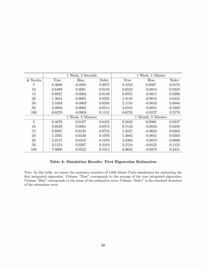
We then apply the realized PCA procedure. We first examine the curse of dimensionality —

20

how increasing number of stocks affects the estimation —and how the sampling frequency affects

the estimation. In light of Corollary 1, we estimate 3 simple integrated eigenvalues as well as

the average of the remaining identical eigenvalues, denoted as∫ t

0 λisds, i = 1, 2, 3, and 4. We

report the mean and standard errors of the estimates as well as the root-mean-square errors of the

standardized estimates with d = 5, 10, 15, 20, 30, 50, and 100 stocks, respectively, using returns

sampled every ∆n = 5 seconds, 1 minute and 5 minutes over one week and one month horizons.

The results, as shown from Tables 2 - 5, suggest that, as expected, the estimation is more diffi cult

as the dimensionality increases, but the large amount of high frequency data and in-fill asymptotic

techniques deliver very satisfactory finite sample approximations. The eigenvalues are accurately

recovered. The repeated eigenvalues are estimated with smaller biases and standard errors, due

to the extra averaging taken at the estimation stage. In Tables 6 - 7, we provide estimates for the

first eigenvectors. Similar to the estimation for eigenvalues, the estimates are very accurate, even

with 100 stocks.

To further verify the accuracy of the asymptotic distribution in small samples as the sample size

increases, we provide in Figure 1 histograms of the standard estimates of integrated eigenvalues

using 30 stocks with 5-second returns. Finally, we examine the finite sample accuracy of the

integrated simple eigenvalues, in the more challenging scenario with 100 stocks sampled every

minute, which matches the setup of the empirical analysis we will conduct below. To verify that

the detection of 3 eigenvalues is not an artifact, we vary the number of common factors in the data

generating process from r = 2 to 4, by removing the third factor or adding another factor that

shares the same parameters as the third factor. The histograms are provided in Figure 2. The

results collectively show that the finite sample performance of the method is quite good even for

a 100-stock portfolio with one-minute returns and one-week horizon.

5 High-Frequency Principal Components in the S&P 100 Stocks

Given the encouraging Monte Carlo results, we now conduct PCA on intraday returns of S&P 100

Index (OEX) constituents. We collect stock prices over the 2003 - 2012 period from the Trade and

Quote (TAQ) database of the New York Stock Exchange (NYSE).4 Due to entry and exit from the

index, there are in total 154 tickers over this 10-year period. We conduct PCA on a weekly basis.

One of the key advantages of the large amount of high frequency data is that we are effectively

able to create a ten-year long time series of eigenvalues and principal components at the weekly

frequency by collating the results obtained over each week in the sample.

After removing those weeks during which the index constituents are switching, we are left with

482 weeks. To clean the data, for each ticker on each trading day, we only keep the intraday prices

4While the constituents of the OEX Index change over time, we keep track of the changes to ensure that ourchoice of stocks is always in line with the index constituents.

21

from the single exchange which has the largest number of transaction records. We provide in

Figure 3 the quantiles of the number of transactions between 9:35 a.m. EST and 3:55 p.m. EST,

across 100 stocks each day. These stocks have excellent liquidity over the sampling period. We

thereby employ 1-minute subsamples for the most liquid 90 stocks in the index (for simplicity, we

still refer to this 90-stock subsample as the S&P 100) in order to address any potential concerns

regarding microstructure noise and asynchronous trading.5 These stocks trade multiple times per

sampling interval and we compute returns using the latest prices recorded within each sampling

interval. Overnight returns are removed so that there is no concern of price changes due to dividend

distributions or stock splits. The 158 time series of cumulative returns are plotted in Figure 4.

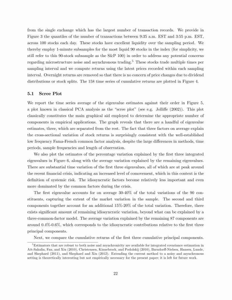
5.1 Scree Plot

We report the time series average of the eigenvalue estimates against their order in Figure 5,

a plot known in classical PCA analysis as the “scree plot” (see e.g. Jolliffe (2002)). This plot

classically constitutes the main graphical aid employed to determine the appropriate number of

components in empirical applications. The graph reveals that there are a handful of eigenvalue

estimates, three, which are separated from the rest. The fact that three factors on average explain

the cross-sectional variation of stock returns is surprisingly consistent with the well-established

low frequency Fama-French common factor analysis, despite the large differences in methods, time

periods, sample frequencies and length of observation.

We also plot the estimates of the percentage variation explained by the first three integrated

eigenvalues in Figure 6, along with the average variation explained by the remaining eigenvalues.

There are substantial time variation of the first three eigenvalues, all of which are at peak around

the recent financial crisis, indicating an increased level of comovement, which in this context is the

definition of systemic risk. The idiosyncratic factors become relatively less important and even

more dominated by the common factors during the crisis.

The first eigenvalue accounts for on average 30-40% of the total variations of the 90 con-

stituents, capturing the extent of the market variation in the sample. The second and third

components together account for an additional 15%-20% of the total variation. Therefore, there

exists significant amount of remaining idiosyncratic variation, beyond what can be explained by a

three-common-factor model. The average variation explained by the remaining 87 components are

around 0.4%-0.6%, which corresponds to the idiosyncratic contributions relative to the first three

principal components.

Next, we compare the cumulative returns of the first three cumulative principal components.

5Estimators that are robust to both noise and asynchronicity are available for integrated covariance estimation inAït-Sahalia, Fan, and Xiu (2010), Christensen, Kinnebrock, and Podolskij (2010), Barndorff-Nielsen, Hansen, Lunde,and Shephard (2011), and Shephard and Xiu (2012). Extending the current method to a noisy and asynchronoussetting is theoretically interesting but not empirically necessary for the present paper; it is left for future work.

22

The time series plots are shown in Figure 7. The empirical correlations among the three components

are -0.020, 0.005, and -0.074, respectively, which agrees with the design that the components are

orthogonal. The first principal component accounts for most of the common variation, and it shares

the time series features of the overall market return. This is further reinforced by the fact that the

loadings of all the stocks on the first principal component, although time-varying, remain positive

throughout the sample period, which is not the case for the additional principal components. It

is worth pointing out however that these principal components are not constrained to be portfolio

returns, as their weights at each point in time are nowhere constrained to add up to one. This

means that the first principal component cannot be taken directly to be the market portfolio, or

more generally identified with additional Fama-French or additional mimicking portfolios.

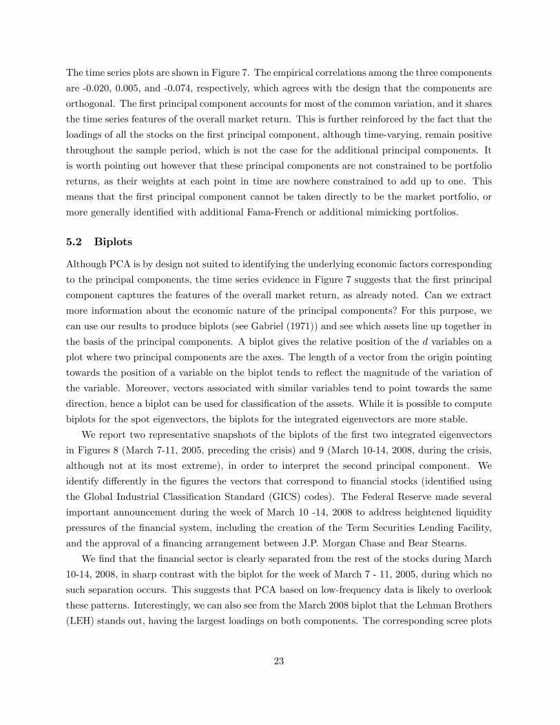
5.2 Biplots

Although PCA is by design not suited to identifying the underlying economic factors corresponding

to the principal components, the time series evidence in Figure 7 suggests that the first principal

component captures the features of the overall market return, as already noted. Can we extract

more information about the economic nature of the principal components? For this purpose, we

can use our results to produce biplots (see Gabriel (1971)) and see which assets line up together in

the basis of the principal components. A biplot gives the relative position of the d variables on a

plot where two principal components are the axes. The length of a vector from the origin pointing

towards the position of a variable on the biplot tends to reflect the magnitude of the variation of

the variable. Moreover, vectors associated with similar variables tend to point towards the same

direction, hence a biplot can be used for classification of the assets. While it is possible to compute

biplots for the spot eigenvectors, the biplots for the integrated eigenvectors are more stable.

We report two representative snapshots of the biplots of the first two integrated eigenvectors

in Figures 8 (March 7-11, 2005, preceding the crisis) and 9 (March 10-14, 2008, during the crisis,

although not at its most extreme), in order to interpret the second principal component. We

identify differently in the figures the vectors that correspond to financial stocks (identified using

the Global Industrial Classification Standard (GICS) codes). The Federal Reserve made several

important announcement during the week of March 10 -14, 2008 to address heightened liquidity

pressures of the financial system, including the creation of the Term Securities Lending Facility,

and the approval of a financing arrangement between J.P. Morgan Chase and Bear Stearns.

We find that the financial sector is clearly separated from the rest of the stocks during March

10-14, 2008, in sharp contrast with the biplot for the week of March 7 - 11, 2005, during which no

such separation occurs. This suggests that PCA based on low-frequency data is likely to overlook

these patterns. Interestingly, we can also see from the March 2008 biplot that the Lehman Brothers

(LEH) stands out, having the largest loadings on both components. The corresponding scree plots

23

for these two weeks in Figures 10 and 11 both suggest the presence of at least three factors, but

the eigenvalues in March 10-14, 2008 are much larger in magnitude, consistently with a higher

systematic component to asset returns. For each week, the figures report 95% confidence intervals

for the first three eigenvalues computed based on the distribution given in Corollary 1.

6 Conclusions

This paper develops the tools necessary to implement PCA at high frequency, constructing and

estimating realized eigenvalues, eigenvectors and principal components. This development comple-

ments the classical PCA theory in a number of ways. Compared to its low frequency counterpart,

PCA becomes feasible over short windows of observation (of the order of one week), relatively large

dimensions (90 in our application) and further are free from the need to impose strong parametric

assumptions on the distribution of the data, applying instead to a broad class of semimartingales.

The estimators perform well in simulations and reveal that the joint dynamics of the S&P 100

stocks at high frequency are well explained by a three-factor model, a result that is broadly consis-

tent with the Fama-French factor model at low frequency, surprisingly so given the large differences

in time scale, sampling and returns horizon.

This paper represents a necessary first step to bring PCA tools to a high frequency setting.

Although not empirically relevant in the context of the analysis above of a portfolio of highly

liquid stocks at the one-minute frequency, the next steps in the development of the theory will

likely include the incorporation of noise-robust and asynchronicity-robust covariance estimation

methods. We hope to pursue these extensions in future work.

24

References

Aït-Sahalia, Y., J. Fan, and D. Xiu (2010): “High-Frequency Covariance Estimates with Noisy andAsynchronous Data,”Journal of the American Statistical Association, 105, 1504—1517.

Aït-Sahalia, Y., and J. Jacod (2014): High Frequency Financial Econometrics. Princeton UniversityPress.

Aït-Sahalia, Y., and D. Xiu (2015): “Using Principal Component Analysis to Estimate a High Di-mensional Factor Model with High-Frequency Data,” Discussion paper, Princeton University and TheUniversity of Chicago.

Amengual, D., and M. W. Watson (2007): “Consistent Estimation of the Number of Dynamic Factorsin a Large N and T Panel,”Journal of Business and Economic Statistics, 25, 91—96.

Amini, A. A., and M. J. Wainwright (2009): “High-Dimensional Analysis of Semidefinite Relaxationsfor Sparse Principal Components,”Annals of Statistics, 37(5B), 2877—2921.

Anderson, T. W. (1958): An Introduction to Multivariate Statistical Analysis. Wiley, New York.

(1963): “Asymptotic Theory for Principal Component Analysis,”Annals of Mathematical Statistics,34, 122—148.

Bai, J. (2003): “Inferential Theory for Factor Models of Large Dimensions,”Econometrica, 71, 135—171.

Bai, J., and S. Ng (2002): “Determining the Number of Factors in Approximate Factor Models,”Econo-metrica, 70, 191—221.

Bai, Z., J. W. Silverstein, and Y. Q. Yin (1988): “A Note on the Largest Eigenvalue of a LargeDimensional Covariance Matrix,”Journal of Multivariate Analysis, 26, 166—168.

Baker, M., and J. Wurgler (2006): “Investor Sentiment and the Cross-Section of Stock Returns,”TheJournal of Finance, 61(4), 1645—1680.

Baker, S. R., N. Bloom, and S. J. Davis (2013): “Measuring Economic Policy Uncertainty,”Discussionpaper, Stanford University and University of Chicago.

Ball, J. M. (1984): “Differentiability Properties of Symmetric and Isotropic Functions,”Duke Mathemat-ical Journal, 51, 699—728.

Barndorff-Nielsen, O. E., P. R. Hansen, A. Lunde, and N. Shephard (2011): “MultivariateRealised Kernels: Consistent Positive Semi-Definite Estimators of the Covariation of Equity Prices withNoise and Non-Synchronous Trading,”Journal of Econometrics, 162, 149—169.

Bickel, P. J., and E. Levina (2008a): “Covariance Regularization by Thresholding,”Annals of Statistics,36(6), 2577—2604.

(2008b): “Regularized Estimation of Large Covariance Matrices,”Annals of Statistics, 36, 199—227.

Brillinger, D. R. (2001): Time Series: Data Analysis and Theory, Classics in Applied Mathematics(Book 36). SIAM: Society for Industrial and Applied Mathematics.

Cai, T. T., and H. H. Zhou (2012): “Optimal Rates of Convergence for Sparse Covariance MatrixEstimation,”Annals of Statistics, 40(5), 2389—2420.

25

Chamberlain, G., and M. Rothschild (1983): “Arbitrage, Factor Structure, and Mean-Variance Analy-sis on Large Asset Markets,”Econometrica, 51, 1281—1304.

Christensen, K., S. Kinnebrock, and M. Podolskij (2010): “Pre-averaging estimators of the ex-postcovariance matrix in noisy diffusion models with non-synchronous data,”Journal of Econometrics, 159,116—133.

Connor, G., and R. Korajczyk (1993): “A test for the number of factors in an approximate factormodel,”The Journal of Finance, 48, 1263—1291.

d’Aspremont, A., L. E. Ghaoui, M. I. Jordan, and G. R. G. Lanckriet (2007): “A Direct Formu-lation for Sparse PCA Using Semidefinite Programming,”SIAM Review, 49(3), 434—448.

Davis, C. (1957): “All Convex Invariant Functions of Hermitian Matrices,”Archiv der Mathematik, 8(4),276—278.

Eaton, M. L., and D. E. Tyler (1991): “On Wielandt’s Inequality and Its Application to the AsymptoticDistribution of the Eigenvalues of A Random Symmetric Matrix,”The Annals of Statistics, 19(1), 260—271.

Egloff, D., M. Leippold, and L. Wu (2010): “The term structure of variance swap rates and optimalvariance swap investments,”Journal of Financial and Quantitative Analysis, 45, 1279—1310.

Fama, E. F., and K. R. French (1993): “Common Risk Factors in the Returns on Stocks and Bonds,”Journal of Financial Economics, 33, 3—56.

Fan, J., A. Furger, and D. Xiu (2016): “Incorporating Global Industrial Classification Standard intoPortfolio Allocation: A Simple Factor-Based Large Covariance Matrix Estimator with High FrequencyData,”Journal of Business and Economic Statistics, 34(4), 489—503.

Friedland, S. (1981): “Convex Spectral Functions,”Linear and Multilinear Algebra, 9, 299—316.

Gabriel, K. (1971): “The biplot graphic display of matrices with application to pricipal componentanalysis,”Biometrika, 58, 453—467.

Geman, S. (1980): “A Limit Theorem for the Norm of RandomMatrices,”Annals of Probability, 8, 252—261.

Hastie, T., R. Tibshirani, and J. Friedman (2009): The Elements of Statistical Learning: Data Mining,Inference, and Prediction, Springer Series in Statistics. Springer-Verlag, New York, second edn.

Heinrich, C., and M. Podolskij (2014): “On Spectral Distribution of High Dimensional CovaraitionMatrices,”Discussion paper, University of Aarhus.

Horn, R. A., and C. R. Johnson (2013): Matrix Analysis. Cambridge University Press, second edn.

Hotelling, H. (1933): “Analysis of a Complex of Statistical Variables into Principal Components,”Journalof Educational Psychology, 24, 417—441, 498—520.

Jackson, J. E. (2003): A User’s Guide to Principal Components. Wiley.

Jacod, J., A. Lejay, and D. Talay (2008): “Estimation of the Brownian dimension of a continuous Itôprocess,”Bernoulli, 14, 469—498.

Jacod, J., and M. Podolskij (2013): “A test for the rank of the volatility process: The RandomPerturbation Approach,”Annals of Statistics, 41, 2391—2427.

Jacod, J., and P. Protter (2012): Discretization of Processes. Springer-Verlag.

26

Jacod, J., and M. Rosenbaum (2013): “Quarticity and Other Functionals of Volatility: Effi cient Esti-mation,”Annals of Statistics, 41, 1462—1484.

Jacod, J., and A. N. Shiryaev (2003): Limit Theorems for Stochastic Processes. Springer-Verlag, secondedn.

Johnstone, I. M. (2001): “On the distribution of the largest eigenvalue in principal components analysis,”Annals of Statistics, 29, 295—327.

Johnstone, I. M., and A. Y. Lu (2009): “On Consistency and Sparsity for Principal ComponentsAnalysis in High Dimensions,”Journal of the American Statistical Association, 104(486), 682—693.

Jolliffe, I. T. (2002): Principal Component Analysis. Springer-Verlag.

Jolliffe, I. T., N. T. Trendafilov, and M. Uddin (2003): “A Modified Principal Component Tech-nique Based on the LASSO,”Journal of Computational and Graphical Statistics, 12(3), 531—547.

Kalnina, I., and D. Xiu (2013): “Model-Free Leverage Effect Estimators at High Frequency,”Discussionpaper, Université de Montréal and University of Chicago.

(2016): “Nonparametric Estimation of the Leverage Effect: A Trade-off Between Robustness andEffi ciency,”Journal of American Statistical Association, forthcoming.

Kapetanios, G. (2010): “A Testing Procedure for Determining the Number of Factors in ApproximateFactor Models,”Journal of Business and Economic Statistics, 28, 397—409.

Lewis, A. S. (1996a): “Convex Analysis on the Hermitian Matrices,”SIAM Journal of Optimizaiton, 6(1),164—177.

(1996b): “Derivatives of Spectral Functions,”Mathematics of Operations Research, 21, 576—588.

Lewis, A. S., and H. S. Sendov (2001): “Twice Differentiable Spectral Functions,” SIAM Journal onMatrix Analysis and Applications, 23, 368—386.

Li, J., V. Todorov, and G. Tauchen (2014): “Adaptive Estimation of Continuous-Time RegressionModels using High-Frequency Data,”Discussion paper, Duke University.

(2016): “Inference Theory on Volatility Functional Dependencies,”Journal of Econometrics, 193,17—34.

Li, J., and D. Xiu (2016): “Generalized Method of Integrated Moments for High-Frequency Data,”Econometrica, 84(4), 1613—1633.

Litterman, R., and J. Scheinkman (1991): “Common factors affecting bond returns,”Journal of FixedIncome, June, 54—61.

Magnus, J. R., and H. Neudecker (1999): Matrix Differential Calculus with Applications in Statisticsand Economics. Wiley.

Mykland, P. A., and L. Zhang (2009): “Inference for continuous semimartingales observed at highfrequency,”Econometrica, 77, 1403—1445.

Okamoto, M. (1973): “Distinctness of the Eigenvalues of a Quadratic form in a Multivariate Sample,”Annals of Statistics, 1, 763—765.

Onatski, A. (2010): “Determining the Number of Factors from Empirical Distribution of Eigenvalues,”Review of Economics and Statistics, 92, 1004—1016.

27

Pearson, K. (1901): “On Lines and Planes of Closest Fit to Systems of Points in Space,”PhilosophicalMagazine, 2, 559—572.

Pelger, M. (2015a): “Large-dimensional factor modeling based on high-frequency observations,”Discus-sion paper, Stanford University.

(2015b): “Understanding Systematic Risk: A High-Frequency Approach,”Discussion paper, Stan-ford University.

Protter, P. (2004): Stochastic Integration and Differential Equations: A New Approach. Springer-Verlag,second edn.

Rockafellar, R. T. (1997): Convex Analysis. Princeton University Press.

Ross, S. A. (1976): “The Arbitrage Theory of Capital Asset Pricing,” Journal of Economic Theory, 13,341—360.

Shephard, N., and D. Xiu (2012): “Econometric analysis of multivariate realized QML: Estimation ofthe covariation of equity prices under asynchronous trading,”Discussion paper, University of Oxford andUniversity of Chicago.

Silhavý, M. (2000): “Differentiability Properties of Isotropic Functions,”Duke Mathematical Journal, 104,367—373.

Stock, J. H., and M. W. Watson (1999): “Forecasting Inflation,”Journal of Monetary Economics, 44,293—335.

(2002a): “Forecasting using Principal Components from a Large Number of Predictors,”Journalof American Statistical Association, 97, 1167—1179.

(2002b): “Macroeconomic Forecasting using Diffusion Indexes,”Journal of Business and EconomicStatistics, 20, 147—162.

Sylvester, J. (1985): “On the Differentiablity of O(n) Invaraint Functions of Symmetric Matrices,”DukeMathematical Journal, 52.

Tao, M., Y. Wang, and X. Chen (2013): “Fast Convergence Rates in Estimating Large VolatilityMatrices Using High-Frequency Financial Data,”Econometric Theory, 29(4), 838—856.

Tao, M., Y. Wang, Q. Yao, and J. Zou (2011): “Large Volatility Matrix Inference via CombiningLow-Frequency and High-Frequency Approaches,”Journal of the American Statistical Association, 106,1025—1040.

Tao, M., Y. Wang, and H. H. Zhou (2013): “Optimal Sparse Volatility Matrix Estimation for High-Dimensional Itô Processes with Measurement Errors,”Annals of Statistics, 41, 1816—1864.

Tao, T. (2012): Topics in Random Matrix Theory. American Mathematical Society.

Tyler, D. E. (1981): “Asymptotic Inference for Eigenvectors,”Annals of Statistics, 9, 725—736.

Wang, Y., and J. Zou (2010): “Vast volatility matrix estimation for high-frequency financial data,”Annals of Statistics, 38, 943—978.

Waternaux, C. M. (1976): “Asymptotic Distribution of the Sample Roots for a Nonnormal Population,”Biometrika, 63, 639—645.

28

Zheng, X., and Y. Li (2011): “On the Estimation of Integrated Covariance Matrices of High DimensionalDiffusion Processes,”Annals of Statistics, 39, 3121—3151.

Zou, H., T. Hastie, and R. Tibshirani (2006): “Sparse Principal Component Analysis,” Journal ofComputational and Graphical Statistics, 15(2), 265—286.

Appendix A Figures and Tables

κj θj ηj ρj µj κj θi,j ξjj = 1 3 0.05 0.3 -0.6 0.05 1 U [0.25, 1.75] 0.5j = 2 4 0.04 0.4 -0.4 0.03 2 N (0, 0.52) 0.6j = 3 5 0.03 0.3 -0.25 0.02 3 N (0, 0.52) 0.7

λF µF+/− λZ µZ+/− µσ2

ρF12 ρF13 ρF23

1/t 4√

∆ 2/t 6√

∆√

∆ 0.05 0.1 0.15κ θ η4 0.3 0.06

Table 1: Parameters in Monte Carlo Simulations

Note: In this table, we report the parameter values used in the simulations. The constant matrix θi,j isgenerated randomly from the described distribution, and is fixed throughout all replications. The dimensionof Xt is 100, whereas the dimension of Ft is 3. ∆ is the sampling frequency, and t is the length of the timewindow. The number of Monte Carlo replications is 1,000.

29

1 Week, 5 Seconds 1 Week, 1 Minute# Stocks True Bias Stdev True Bias Stdev

5 0.4686 -0.0001 0.0075 0.4703 0.0007 0.015210 0.6489 0.0001 0.0110 0.6552 -0.0014 0.022315 0.8927 -0.0004 0.0149 0.8975 -0.0011 0.029620 1.3044 0.0003 0.0225 1.3148 -0.0018 0.042430 2.1003 -0.0002 0.0356 2.1134 -0.0033 0.068850 2.9863 0.0002 0.0514 3.0104 -0.0054 0.1002100 6.6270 -0.0004 0.1141 6.6732 -0.0127 0.2179

1 Week, 5 Minutes 1 Month, 5 Minutes5 0.4879 0.0107 0.0452 0.5642 0.0006 0.024710 0.6839 0.0084 0.0574 0.7143 -0.0024 0.025815 0.9397 0.0128 0.0724 1.0167 -0.0024 0.038220 1.3765 0.0130 0.1076 1.3882 -0.0041 0.050330 2.2157 0.0210 0.1670 2.2383 -0.0073 0.080650 3.1554 0.0267 0.2410 3.1518 -0.0125 0.1155100 7.0000 0.0552 0.5314 6.9632 -0.0270 0.2451

Table 2: Simulation Results: First Eigenvalue Estimation

Note: In this table, we report the summary statistics of 1,000 Monte Carlo simulations for estimating thefirst integrated eigenvalue. Column “True” corresponds to the average of the true integrated eigenvalue;Column “Bias”corresponds to the mean of the estimation error; Column “Stdev”is the standard deviationof the estimation error.

30

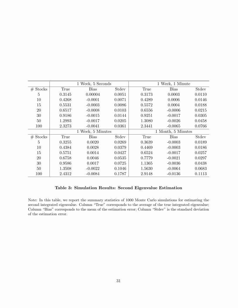
1 Week, 5 Seconds 1 Week, 1 Minute# Stocks True Bias Stdev True Bias Stdev

5 0.3145 0.00004 0.0051 0.3173 0.0003 0.011010 0.4268 -0.0001 0.0071 0.4289 0.0006 0.014615 0.5531 -0.0003 0.0086 0.5572 0.0004 0.018820 0.6517 -0.0008 0.0103 0.6556 -0.0006 0.021530 0.9186 -0.0015 0.0144 0.9251 -0.0017 0.030550 1.2993 -0.0017 0.0205 1.3080 -0.0026 0.0458100 2.3273 -0.0041 0.0361 2.3441 -0.0065 0.0766

1 Week, 5 Minutes 1 Month, 5 Minutes# Stocks True Bias Stdev True Bias Stdev

5 0.3255 0.0020 0.0269 0.3639 -0.0003 0.018910 0.4384 0.0028 0.0379 0.4469 -0.0003 0.018615 0.5751 0.0014 0.0427 0.6524 -0.0017 0.025720 0.6758 0.0046 0.0535 0.7779 -0.0021 0.029730 0.9586 0.0017 0.0725 1.1365 -0.0036 0.043850 1.3508 -0.0022 0.1046 1.5630 -0.0064 0.0683100 2.4312 -0.0084 0.1787 2.9148 -0.0136 0.1113

Table 3: Simulation Results: Second Eigenvalue Estimation

Note: In this table, we report the summary statistics of 1000 Monte Carlo simulations for estimating thesecond integrated eigenvalue. Column “True”corresponds to the average of the true integrated eigenvalue;Column “Bias”corresponds to the mean of the estimation error; Column “Stdev”is the standard deviationof the estimation error.

31

1 Week, 5 Seconds 1 Week, 1 Minute# Stocks True Bias Stdev True Bias Stdev

5 0.1338 0.0001 0.0022 0.1345 0.0003 0.004410 0.2132 0.0001 0.0035 0.2149 0.0002 0.007015 0.2941 0.0002 0.0046 0.2954 0.0002 0.009320 0.3212 0.0001 0.0052 0.3242 0.0000 0.010530 0.4825 0.0005 0.0078 0.4853 0.0001 0.015350 0.6943 0.0001 0.0113 0.7016 -0.0005 0.0226100 1.3808 0.0004 0.0221 1.3935 -0.0013 0.0438

1 Week, 5 Minutes 1 Month, 5 Minutes# Stocks True Bias Stdev True Bias Stdev

5 0.1364 0.0041 0.0124 0.1404 0.0006 0.005410 0.2199 0.0033 0.0183 0.2367 -0.0001 0.009115 0.3018 0.0056 0.0264 0.3396 0.0009 0.013120 0.3324 0.0037 0.0294 0.3546 0.0003 0.013230 0.4971 0.0055 0.0409 0.5686 0.0006 0.021150 0.7216 0.0028 0.0577 0.8051 -0.0010 0.0306100 1.4302 -0.0016 0.1119 1.6278 -0.0028 0.0612

Table 4: Simulation Results: Third Eigenvalue Estimation

Note: In this table, we report the summary statistics of 1,000 Monte Carlo simulations for estimating thethird integrated eigenvalue. Column “True”corresponds to the average of the true integrated eigenvalue;Column “Bias”corresponds to the mean of the estimation error; Column “Stdev”is the standard deviationof the estimation error.

32

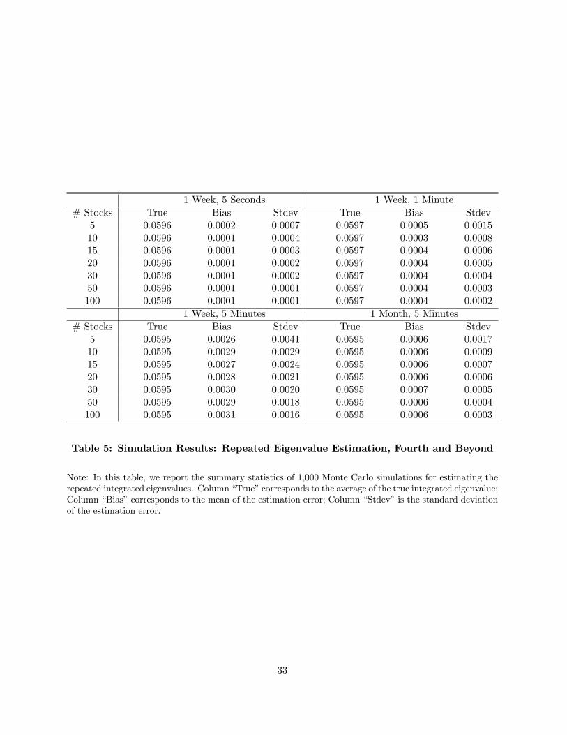
1 Week, 5 Seconds 1 Week, 1 Minute# Stocks True Bias Stdev True Bias Stdev

5 0.0596 0.0002 0.0007 0.0597 0.0005 0.001510 0.0596 0.0001 0.0004 0.0597 0.0003 0.000815 0.0596 0.0001 0.0003 0.0597 0.0004 0.000620 0.0596 0.0001 0.0002 0.0597 0.0004 0.000530 0.0596 0.0001 0.0002 0.0597 0.0004 0.000450 0.0596 0.0001 0.0001 0.0597 0.0004 0.0003100 0.0596 0.0001 0.0001 0.0597 0.0004 0.0002

1 Week, 5 Minutes 1 Month, 5 Minutes# Stocks True Bias Stdev True Bias Stdev

5 0.0595 0.0026 0.0041 0.0595 0.0006 0.001710 0.0595 0.0029 0.0029 0.0595 0.0006 0.000915 0.0595 0.0027 0.0024 0.0595 0.0006 0.000720 0.0595 0.0028 0.0021 0.0595 0.0006 0.000630 0.0595 0.0030 0.0020 0.0595 0.0007 0.000550 0.0595 0.0029 0.0018 0.0595 0.0006 0.0004100 0.0595 0.0031 0.0016 0.0595 0.0006 0.0003

Table 5: Simulation Results: Repeated Eigenvalue Estimation, Fourth and Beyond

Note: In this table, we report the summary statistics of 1,000 Monte Carlo simulations for estimating therepeated integrated eigenvalues. Column “True”corresponds to the average of the true integrated eigenvalue;Column “Bias”corresponds to the mean of the estimation error; Column “Stdev”is the standard deviationof the estimation error.

33

1 Week, 5 Seconds 1 Week, 1 Minute# Stocks True Bias Stdev True Bias Stdev

0.2457 -0.0002 0.0173 0.2475 0.0074 0.15590.8987 0.0028 0.0261 0.8963 0.0174 0.2135

5 0.0566 0.0013 0.0235 0.0536 -0.0018 0.12810.0633 0.0001 0.0119 0.0639 0.0037 0.07860.3110 0.0017 0.0202 0.3086 0.0042 0.06450.0506 0.0004 0.0049 0.0495 0.0029 0.02660.3444 0.0006 0.0087 0.3452 0.0080 0.06910.4632 0.0011 0.0129 0.4619 0.0121 0.09660.1422 0.0008 0.0137 0.1422 0.0094 0.0990

10 0.4166 0.0004 0.0220 0.4164 0.0045 0.15620.0864 0.0008 0.0158 0.0863 0.0089 0.11170.3460 0.0008 0.0088 0.3440 0.0101 0.06000.1268 0.0005 0.0076 0.1259 0.0066 0.04510.3409 0.0005 0.0174 0.3415 0.0046 0.12680.4262 0.0007 0.0112 0.4271 0.0099 0.0942

Table 6: Simulation Results: Eigenvector Estimation

Note: In this table, we report the summary statistics of 1,000 Monte Carlo simulations for estimating theintegrated eigenvector associated with the first eigenvalue. Column “True”corresponds to the average of thetrue integrated vector; Column “Bias”corresponds to the mean of the estimation error; Column “Stdev”isthe standard deviation of the estimation error. The setup for these simulations is identical to that of Tables2-5.

34

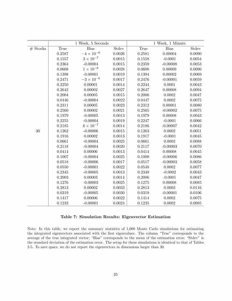
1 Week, 5 Seconds 1 Week, 1 Minute# Stocks True Bias Stdev True Bias Stdev

0.2587 −4× 10−6 0.0026 0.2581 0.00004 0.00900.1557 3× 10−7 0.0015 0.1558 -0.0001 0.00540.2364 -0.00004 0.0015 0.2359 -0.00008 0.00530.0608 1× 10−6 0.0028 0.0608 0.00009 0.00960.1398 -0.00001 0.0019 0.1394 0.00002 0.00690.2471 −3× 10−6 0.0017 0.2476 -0.00001 0.00590.2250 0.00001 0.0014 0.2244 0.0001 0.00430.2642 0.00002 0.0027 0.2647 0.00008 0.00940.2004 0.00005 0.0015 0.2006 0.0002 0.00470.0446 -0.00004 0.0022 0.0447 0.0002 0.00750.2311 0.00005 0.0023 0.2312 0.00001 0.00800.2560 0.00002 0.0021 0.2565 -0.00002 0.00750.1979 -0.00005 0.0013 0.1979 0.00008 0.00430.2255 -0.00004 0.0019 0.2247 -0.0001 0.00660.2185 6× 10−7 0.0014 0.2186 -0.00007 0.0042

30 0.1262 -0.00006 0.0015 0.1263 0.0002 0.00510.1916 0.00002 0.0013 0.1917 -0.0001 0.00450.0661 -0.00004 0.0025 0.0661 0.0002 0.00880.2118 -0.00004 0.0020 0.2117 -0.00003 0.00700.0414 0.00006 0.0013 0.0414 0.00008 0.00450.1007 -0.00004 0.0025 0.1008 -0.00006 0.00860.0518 -0.00006 0.0017 0.0517 -0.00003 0.00580.0550 -0.00001 0.0022 0.0548 0.0002 0.00770.2345 -0.00005 0.0013 0.2349 -0.0002 0.00430.2003 0.00003 0.0014 0.2006 -0.0001 0.00470.1276 -0.00003 0.0025 0.1275 0.00008 0.00850.2813 0.00002 0.0033 0.2813 0.0003 0.01160.0319 -0.00005 0.0030 0.0319 -0.00001 0.01060.1417 0.00006 0.0022 0.1414 0.0002 0.00750.1233 -0.00001 0.0024 0.1235 0.0002 0.0085

Table 7: Simulation Results: Eigenvector Estimation

Note: In this table, we report the summary statistics of 1,000 Monte Carlo simulations for estimatingthe integrated eigenvectors associated with the first eigenvalues. The column “True” corresponds to theaverage of the true integrated vector; “Bias” corresponds to the mean of the estimation error; “Stdev” isthe standard deviation of the estimation error. The setup for these simulations is identical to that of Tables2-5. To save space, we do not report the eigenvectors in dimensions larger than 30.

35

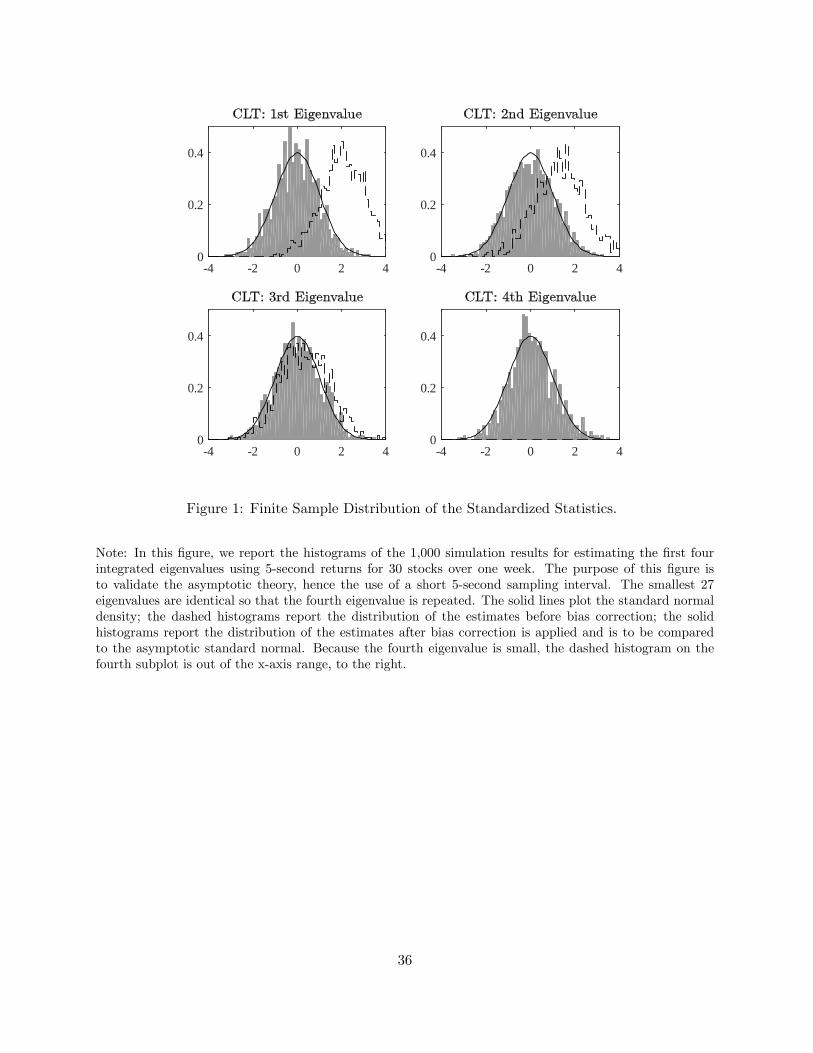
­4 ­2 0 2 4 0

0.2

0.4

­4 ­2 0 2 4 0

0.2

0.4

­4 ­2 0 2 4 0

0.2

0.4

­4 ­2 0 2 4 0

0.2

0.4

Figure 1: Finite Sample Distribution of the Standardized Statistics.

Note: In this figure, we report the histograms of the 1,000 simulation results for estimating the first fourintegrated eigenvalues using 5-second returns for 30 stocks over one week. The purpose of this figure isto validate the asymptotic theory, hence the use of a short 5-second sampling interval. The smallest 27eigenvalues are identical so that the fourth eigenvalue is repeated. The solid lines plot the standard normaldensity; the dashed histograms report the distribution of the estimates before bias correction; the solidhistograms report the distribution of the estimates after bias correction is applied and is to be comparedto the asymptotic standard normal. Because the fourth eigenvalue is small, the dashed histogram on thefourth subplot is out of the x-axis range, to the right.

36

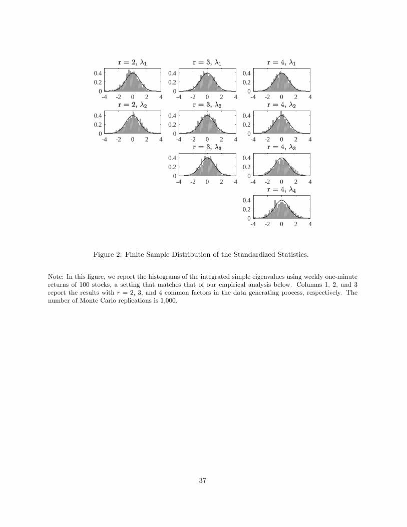
­4 ­2 0 2 4 0

0.20.4

­4 ­2 0 2 4 0

0.20.4

­4 ­2 0 2 4 0

0.20.4

­4 ­2 0 2 4 0

0.20.4

­4 ­2 0 2 4 0

0.20.4

­4 ­2 0 2 4 0

0.20.4

­4 ­2 0 2 4 0

0.20.4

­4 ­2 0 2 4 0

0.20.4

­4 ­2 0 2 4 0

0.20.4

Figure 2: Finite Sample Distribution of the Standardized Statistics.

Note: In this figure, we report the histograms of the integrated simple eigenvalues using weekly one-minutereturns of 100 stocks, a setting that matches that of our empirical analysis below. Columns 1, 2, and 3report the results with r = 2, 3, and 4 common factors in the data generating process, respectively. Thenumber of Monte Carlo replications is 1,000.

37

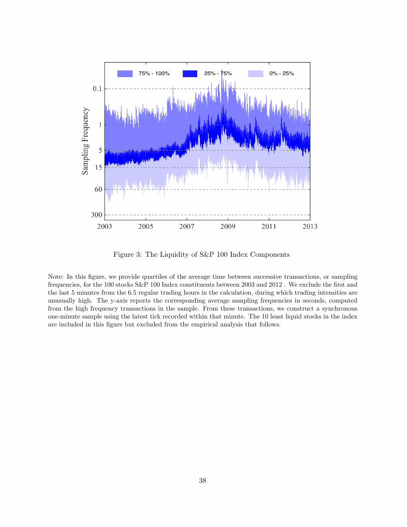
Figure 3: The Liquidity of S&P 100 Index Components

Note: In this figure, we provide quartiles of the average time between successive transactions, or samplingfrequencies, for the 100 stocks S&P 100 Index constituents between 2003 and 2012 . We exclude the first andthe last 5 minutes from the 6.5 regular trading hours in the calculation, during which trading intensities areunusually high. The y-axis reports the corresponding average sampling frequencies in seconds, computedfrom the high frequency transactions in the sample. From these transactions, we construct a synchronousone-minute sample using the latest tick recorded within that minute. The 10 least liquid stocks in the indexare included in this figure but excluded from the empirical analysis that follows.

38

Figure 4: Time Series of the Cumulative Returns of S&P 100 Index Components

Note: In this figure, we plot the time series of cumulative daily open-to-close returns of 158 S&P 100 IndexComponents from 2003 to 2012. The thick black solid line plots the cumulative daily open-to-close S&P100 Index returns. All overnight returns are excluded. Companies that exited the index during the sampleperiod, including bankruptcies, are represented by a time series truncated at the time of delisting.

39

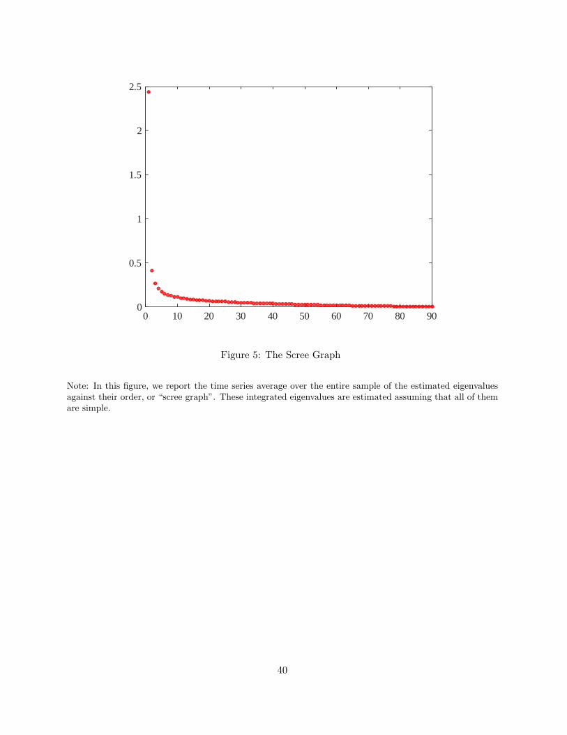
0 10 20 30 40 50 60 70 80 900

0.5

1

1.5

2

2.5

Figure 5: The Scree Graph

Note: In this figure, we report the time series average over the entire sample of the estimated eigenvaluesagainst their order, or “scree graph”. These integrated eigenvalues are estimated assuming that all of themare simple.

40

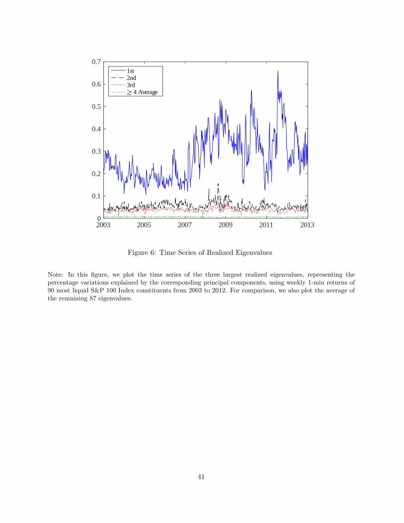
2003 2005 2007 2009 2011 2013 0

0.1

0.2

0.3

0.4

0.5

0.6

0.71st2nd3rd

4 Average

Figure 6: Time Series of Realized Eigenvalues

Note: In this figure, we plot the time series of the three largest realized eigenvalues, representing thepercentage variations explained by the corresponding principal components, using weekly 1-min returns of90 most liquid S&P 100 Index constituents from 2003 to 2012. For comparison, we also plot the average ofthe remaining 87 eigenvalues.

41

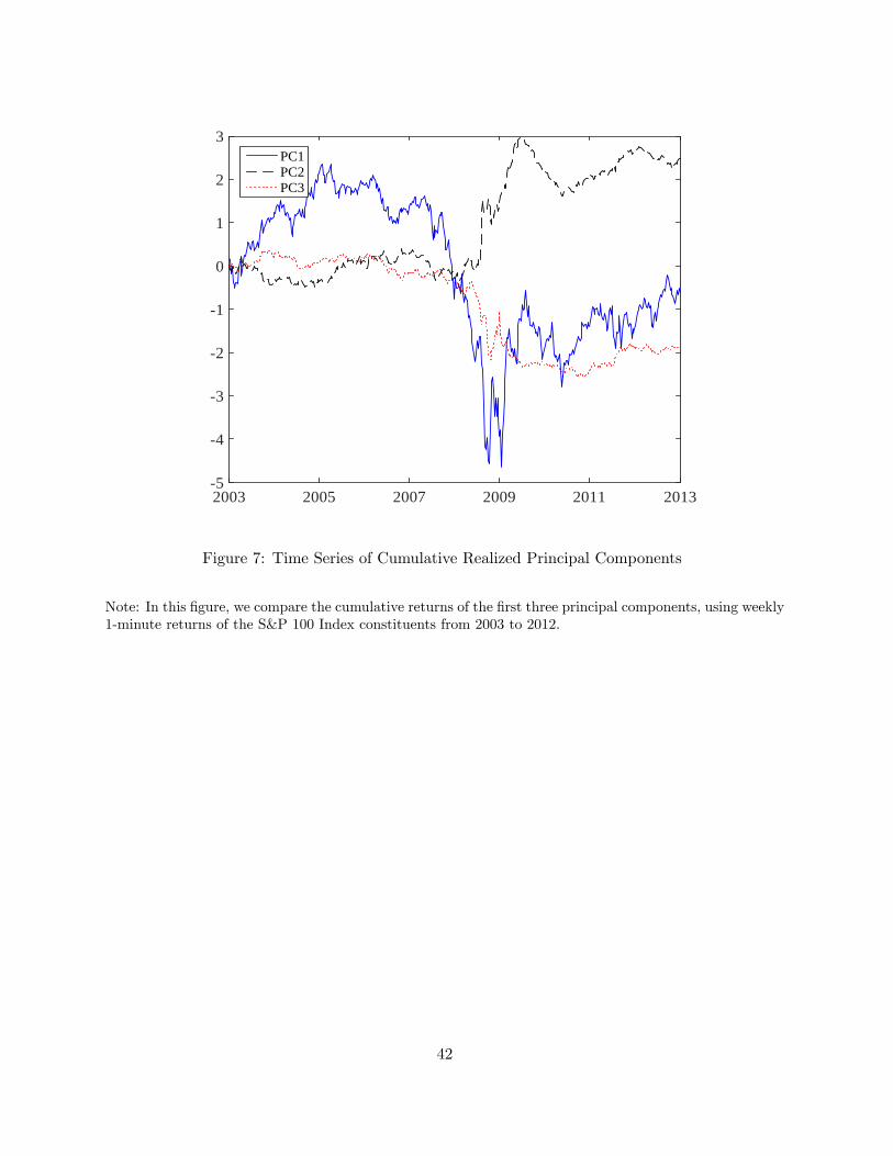
2003 2005 2007 2009 2011 2013­5

­4

­3

­2

­1

0

1

2

3PC1PC2PC3

Figure 7: Time Series of Cumulative Realized Principal Components

Note: In this figure, we compare the cumulative returns of the first three principal components, using weekly1-minute returns of the S&P 100 Index constituents from 2003 to 2012.

42

Component 10 0.05 0.1 0.15 0.2 0.25

Com

pone

nt 2

­0.12

­0.1

­0.08

­0.06

­0.04

­0.02

0

0.02

0.04

0.06Week: 03/07/2005 ­­ 03/11/2005

Non­FinancialFinancial

Figure 8: Biplot of the Integrated Eigenvector: Pre-Crisis Week

Note: This biplot shows the integrated eigenvector estimated during the week March 7-11, 2005. Each dotand the vector joining it and the origin represents a firm. The x and y coordinates of a firm denote itsaverage loading on the first and second principal components, respectively. The dots and lines associatedwith firms in the financial sector are colored in red and dashed, while non-financial firms are colored in blueand drawn as solid lines. The figures shows little difference between the two groups during that week.

43

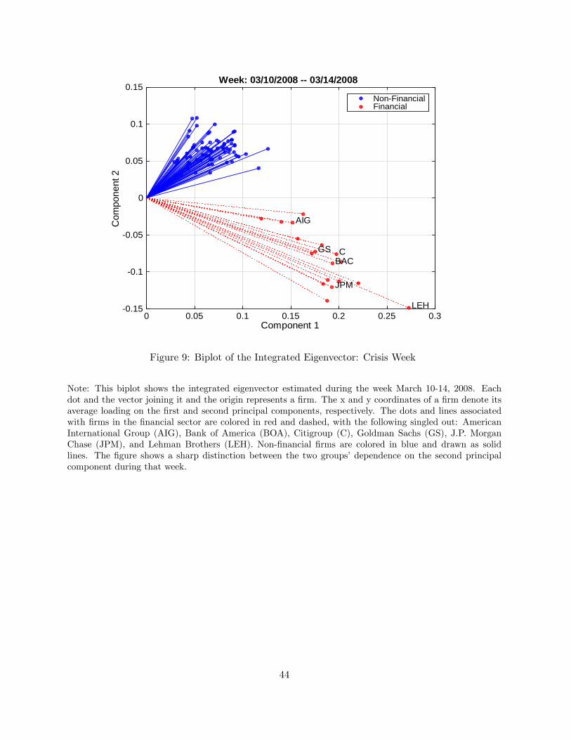
Component 10 0.05 0.1 0.15 0.2 0.25 0.3

Com

pone

nt 2

­0.15

­0.1

­0.05

0

0.05

0.1

0.15

AIG

CGSBAC

JPM

LEH

Week: 03/10/2008 ­­ 03/14/2008

Non­FinancialFinancial

Figure 9: Biplot of the Integrated Eigenvector: Crisis Week

Note: This biplot shows the integrated eigenvector estimated during the week March 10-14, 2008. Eachdot and the vector joining it and the origin represents a firm. The x and y coordinates of a firm denote itsaverage loading on the first and second principal components, respectively. The dots and lines associatedwith firms in the financial sector are colored in red and dashed, with the following singled out: AmericanInternational Group (AIG), Bank of America (BOA), Citigroup (C), Goldman Sachs (GS), J.P. MorganChase (JPM), and Lehman Brothers (LEH). Non-financial firms are colored in blue and drawn as solidlines. The figure shows a sharp distinction between the two groups’dependence on the second principalcomponent during that week.

44

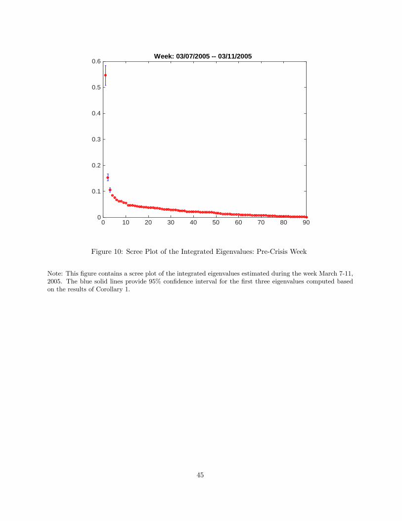
0 10 20 30 40 50 60 70 80 900

0.1

0.2

0.3

0.4

0.5

0.6Week: 03/07/2005 ­­ 03/11/2005

Figure 10: Scree Plot of the Integrated Eigenvalues: Pre-Crisis Week

Note: This figure contains a scree plot of the integrated eigenvalues estimated during the week March 7-11,2005. The blue solid lines provide 95% confidence interval for the first three eigenvalues computed basedon the results of Corollary 1.

45

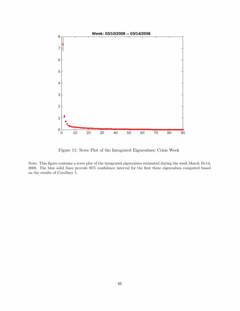
0 10 20 30 40 50 60 70 80 900

1

2

3

4

5

6

7

8Week: 03/10/2008 ­­ 03/14/2008

Figure 11: Scree Plot of the Integrated Eigenvalues: Crisis Week

Note: This figure contains a scree plot of the integrated eigenvalues estimated during the week March 10-14,2008. The blue solid lines provide 95% confidence interval for the first three eigenvalues computed basedon the results of Corollary 1.

46

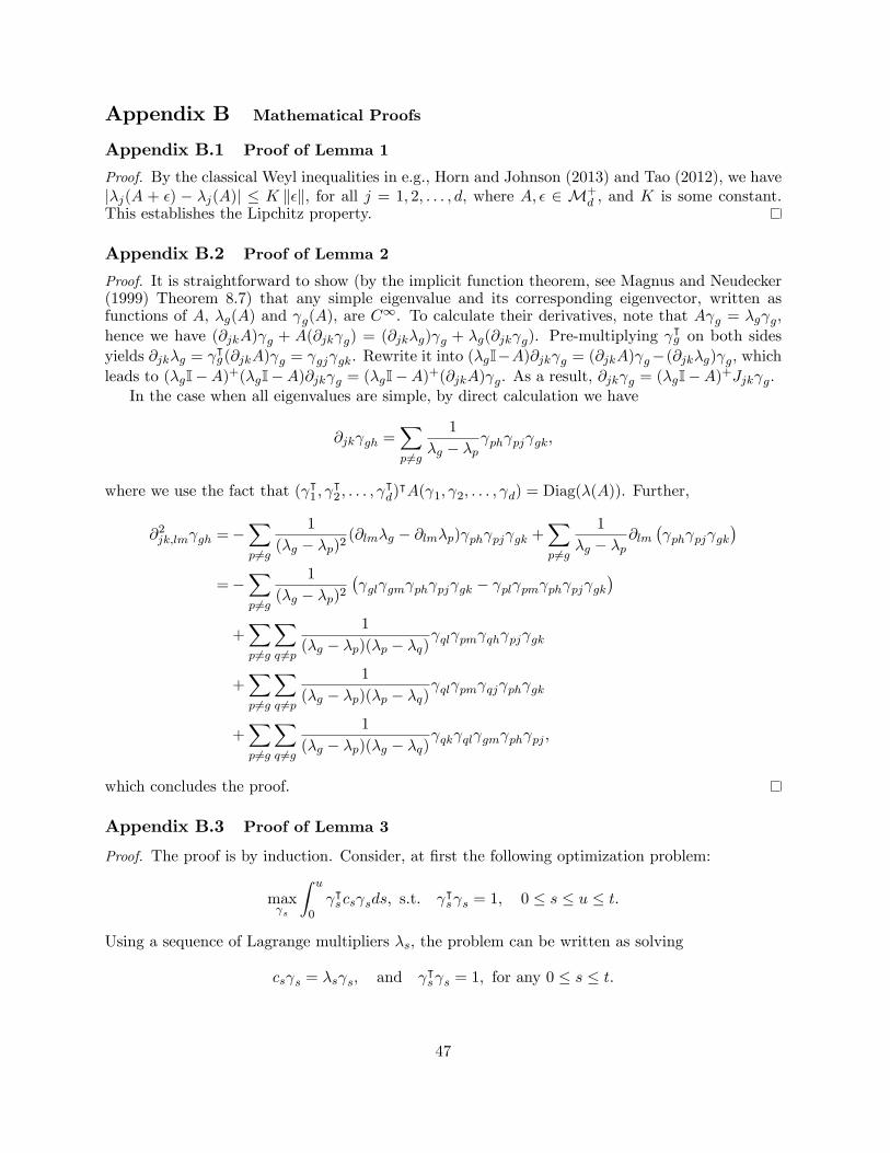
Appendix B Mathematical Proofs

Appendix B.1 Proof of Lemma 1

Proof. By the classical Weyl inequalities in e.g., Horn and Johnson (2013) and Tao (2012), we have|λj(A + ε) − λj(A)| ≤ K ‖ε‖, for all j = 1, 2, . . . , d, where A, ε ∈ M+

d , and K is some constant.This establishes the Lipchitz property.

Appendix B.2 Proof of Lemma 2

Proof. It is straightforward to show (by the implicit function theorem, see Magnus and Neudecker(1999) Theorem 8.7) that any simple eigenvalue and its corresponding eigenvector, written asfunctions of A, λg(A) and γg(A), are C∞. To calculate their derivatives, note that Aγg = λgγg,hence we have (∂jkA)γg + A(∂jkγg) = (∂jkλg)γg + λg(∂jkγg). Pre-multiplying γ

ᵀg on both sides

yields ∂jkλg = γᵀg(∂jkA)γg = γgjγgk. Rewrite it into (λgI−A)∂jkγg = (∂jkA)γg−(∂jkλg)γg, whichleads to (λgI−A)+(λgI−A)∂jkγg = (λgI−A)+(∂jkA)γg. As a result, ∂jkγg = (λgI−A)+Jjkγg.

In the case when all eigenvalues are simple, by direct calculation we have

∂jkγgh =∑p 6=g

1

λg − λpγphγpjγgk,

where we use the fact that (γᵀ1 , γᵀ2 , . . . , γ

ᵀd)ᵀA(γ1, γ2, . . . , γd) = Diag(λ(A)). Further,

∂2jk,lmγgh =−

∑p6=g

1

(λg − λp)2(∂lmλg − ∂lmλp)γphγpjγgk +

∑p 6=g

1

λg − λp∂lm

(γphγpjγgk

)=−

∑p6=g

1

(λg − λp)2

(γglγgmγphγpjγgk − γplγpmγphγpjγgk

)+∑p6=g

∑q 6=p

1

(λg − λp)(λp − λq)γqlγpmγqhγpjγgk

+∑p6=g

∑q 6=p

1

(λg − λp)(λp − λq)γqlγpmγqjγphγgk

+∑p6=g

∑q 6=g

1

(λg − λp)(λg − λq)γqkγqlγgmγphγpj ,

which concludes the proof.

Appendix B.3 Proof of Lemma 3

Proof. The proof is by induction. Consider, at first the following optimization problem:

maxγs

∫ u

0γᵀscsγsds, s.t. γᵀsγs = 1, 0 ≤ s ≤ u ≤ t.

Using a sequence of Lagrange multipliers λs, the problem can be written as solving

csγs = λsγs, and γᵀsγs = 1, for any 0 ≤ s ≤ t.

47

Hence, the original problem is translated into eigenanalysis.Suppose the eigenvalues of cs are ordered as in λ1,s ≥ λ2,s ≥ . . . ≥ λd,s. Note that γᵀscsγs = λs,

so that λs = λ1,s, and γs = γ1,s is one of the corresponding eigenvectors (if λ1,s is not unique),

and the maximal variation is∫ t

0 λ1,sds.Suppose that we have found γ1,s, . . . , γk,s, for 1 ≤ k < d and 0 ≤ s ≤ t, the (k+ 1)th principal

component is defined by solving the following problem:

maxγs

∫ u

0γᵀscsγsds, s.t. γᵀsγs = 1, and γᵀj,scsγs = 0, for 1 ≤ j ≤ k, 0 ≤ u ≤ t.

Using similar technique of Lagrange multipliers, λs, and ν1,s, . . . , νk,s, we find

csγs = λsγs +

k∑j=1

νj,scsγj,s.

Multiplying on the left γᵀl,s, for some 1 ≤ l ≤ k, we can show that νl,scsγl,s = 0. Indeed,

0 = λl,sγᵀl,sγs = γᵀl,scsγs = γᵀl,sλsγs +

k∑j=1

νj,sγᵀl,scsγj,s = νl,sλl,s.

Therefore, since l is an arbitrary number between 1 and k, we have csγs = λsγs. Hence, λs = λk+1,s,γs = γk+1,s is one of the eigenvectors associated with the eigenvalue λk+1,s. This establishes thefirst part of the theorem.

For any càdlàg and adapted process γs,[∫ u

0γᵀs−dXs,

∫ u

0γᵀs−dXs

]c=

∫ t

0γᵀscsγsds.

Hence the statement follows from the gth-step optimization problem. Note that the validity of theintegrals above is warranted by the continuity of λ given by Lemma 1.

Appendix B.4 Proof of Lemma 4

Proof. The first statement of the proof follows by immediate calculations from Theorem 1.1 inLewis (1996b) and Theorem 3.3 in Lewis and Sendov (2001). The second statement is discussedand proved in, e.g., Ball (1984), Sylvester (1985), and Silhavý (2000). Finally, the last statementon convexity is proved in Davis (1957) and Lewis (1996a).

Appendix B.5 Proof of Lemma 5

Proof. Obviously, for any 1 ≤ g1 < g2 < . . . < gr ≤ d, the set defined in (4), D(g1, g2, . . . , gr),is an open set in R+

d /0. Define f(x) = |xgr | +∑

i 6=j |xgi − xgj |, which is a continuous andconvex function. It is differentiable at x if and only if x ∈ D(g1, g2, . . . , gr). Therefore, byLemma 4, f λ is convex, and it is differentiable at A if and only if λ(A) ∈ D(g1, g2, . . . , gr),i.e., A ∈ M(g1, g2, . . . , gr). On the other hand, a convex function is almost everywhere differen-tiable, see Rockafellar (1997), which implies that M(g1, g2, . . . , gr) is dense in M++

d . Moreover,M(g1, g2, . . . , gr) is the pre-image of the open set R+/0 under a continuous function hλ, whereh(x) =

∏i 6=j |xgi − xgj ||xgr |. Therefore, it is open.

48

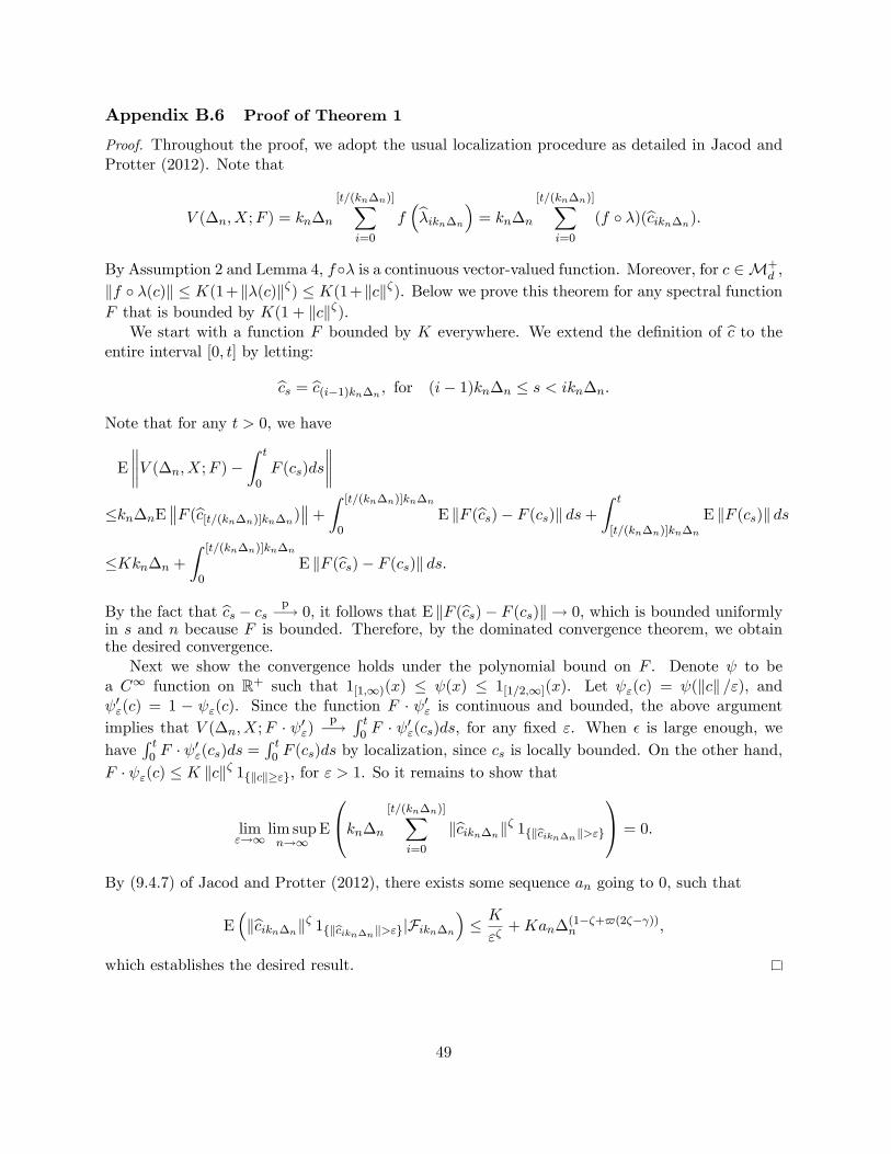
Appendix B.6 Proof of Theorem 1

Proof. Throughout the proof, we adopt the usual localization procedure as detailed in Jacod andProtter (2012). Note that

V (∆n, X;F ) = kn∆n

[t/(kn∆n)]∑i=0

f(λikn∆n

)= kn∆n

[t/(kn∆n)]∑i=0

(f λ)(cikn∆n).

By Assumption 2 and Lemma 4, fλ is a continuous vector-valued function. Moreover, for c ∈M+d ,

‖f λ(c)‖ ≤ K(1+‖λ(c)‖ζ) ≤ K(1+‖c‖ζ). Below we prove this theorem for any spectral functionF that is bounded by K(1 + ‖c‖ζ).

We start with a function F bounded by K everywhere. We extend the definition of c to theentire interval [0, t] by letting:

cs = c(i−1)kn∆n, for (i− 1)kn∆n ≤ s < ikn∆n.

Note that for any t > 0, we have

E

∥∥∥∥V (∆n, X;F )−∫ t

0F (cs)ds

∥∥∥∥≤kn∆nE

∥∥F (c[t/(kn∆n)]kn∆n)∥∥+

∫ [t/(kn∆n)]kn∆n

0E ‖F (cs)− F (cs)‖ ds+

∫ t

[t/(kn∆n)]kn∆n

E ‖F (cs)‖ ds

≤Kkn∆n +

∫ [t/(kn∆n)]kn∆n

0E ‖F (cs)− F (cs)‖ ds.

By the fact that cs − csp−→ 0, it follows that E ‖F (cs)− F (cs)‖ → 0, which is bounded uniformly

in s and n because F is bounded. Therefore, by the dominated convergence theorem, we obtainthe desired convergence.

Next we show the convergence holds under the polynomial bound on F . Denote ψ to bea C∞ function on R+ such that 1[1,∞)(x) ≤ ψ(x) ≤ 1[1/2,∞](x). Let ψε(c) = ψ(‖c‖ /ε), andψ′ε(c) = 1 − ψε(c). Since the function F · ψ′ε is continuous and bounded, the above argumentimplies that V (∆n, X;F · ψ′ε)

p−→∫ t

0 F · ψ′ε(cs)ds, for any fixed ε. When ε is large enough, we

have∫ t

0 F · ψ′ε(cs)ds =

∫ t0 F (cs)ds by localization, since cs is locally bounded. On the other hand,

F · ψε(c) ≤ K ‖c‖ζ 1‖c‖≥ε, for ε > 1. So it remains to show that

limε→∞

lim supn→∞

E

kn∆n

[t/(kn∆n)]∑i=0

‖cikn∆n‖ζ 1‖cikn∆n‖>ε

= 0.

By (9.4.7) of Jacod and Protter (2012), there exists some sequence an going to 0, such that

E(‖cikn∆n‖

ζ 1‖cikn∆n‖>ε|Fikn∆n

)≤ K

εζ+Kan∆(1−ζ+$(2ζ−γ))

n ,

which establishes the desired result.

49

Appendix B.7 Proof of Proposition 1

Proof. We divide the proof into several steps. To start, we need some additional notations. LetX ′ and c′ denote the continuous parts of the processes X and c, respectively. Also, we introducec′ikn∆n

to denote the estimator constructed similarly as in (5) with X replaced by X ′ and withouttruncation, namely

c′ikn∆n=

1

kn∆n

kn∑j=1

(∆nikn+jX

′)(∆nikn+jX

′)ᵀ.

In addition, λ′ikn∆n

corresponds to the vector of eigenvalues of c′ikn∆n, and

V ′(∆n, X;F ) = kn∆n

[t/(kn∆n)]∑i=0

f(λ′ikn∆n

).

We also define

cikn∆n =1

kn∆n

∫ (i+1)kn∆n

ikn∆n

csds, βnikn = c′ikn∆n− cikn∆n , αnl = (∆n

l X′)(∆n

l X′)ᵀ − cl∆n∆n, and

ηni =

(E

(sup

i∆n≤u≤i∆n+kn∆n

|bi∆n+u − bi∆n |2|Fi∆n

))1/2

.

We first collect some known estimates in the next lemma:

Lemma 6. Under the assumptions of Proposition 1, we have

E

(sup

0≤u≤s‖ct+u − ct‖q |Ft

)≤ Ks1∧q/2, ‖E (ct+s − ct|Ft)‖ ≤ Ks, (B.1)

E∥∥∥(∆n

i X)(∆ni X)ᵀ1‖∆n

i X‖≤un − (∆ni X′)(∆n

i X′)ᵀ∥∥∥ ≤ Kan∆(2−γ)$+1

n , for some an → 0, (B.2)

E(∥∥cikn∆n − c′ikn∆n

∥∥q) ≤ Kan∆(2q−γ)$+1−qn , for some q ≥ 1, and an → 0, (B.3)

E∥∥c′ikn∆n

− cikn∆n

∥∥p ≤ Kk−p/2n , for some p ≥ 1, (B.4)

E (‖αni ‖q |Fi∆n) ≤ K∆q

n, for some q ≥ 0, (B.5)

‖E (αni |Fi∆n)‖ ≤ K∆3/2n

(∆1/2n + ηni

), (B.6)∣∣∣E(αn,jki αn,lmi −

(cjli∆n

ckmi∆n+ cjmi∆n

ckli∆n

)∆2n|Fi∆n

)∣∣∣ ≤ K∆5/2n , (B.7)∥∥E

(βnikn |Fikn∆n

)∥∥ ≤ K∆n1/2(kn∆1/2

n + ηnikn

), (B.8)∥∥∥E

(βn,jkikn

βn,lmikn|Fikn∆n

)− k−1

n (cjlikn∆nckmikn∆n

+ cjmikn∆ncklikn∆n

)∥∥∥

≤ K∆n1/2(k−1/2n + kn∆1/2

n + ηnikn

), (B.9)

E(∥∥βnikn∥∥q |Fikn∆n

)≤ K

(k−q/2n + kn∆n

), for some q ≥ 2, (B.10)

∆nE

[t/∆n]∑i=1

ηni → 0. (B.11)

50

Proof of Lemma 6. These estimates are given by Lemma A.2 in Li and Xiu (2016), (4.3), (4.8),(4.10), (4.11), (4.12), (4.18), Lemmas 4.2 and 4.3 of Jacod and Rosenbaum (2013), and Lemma13.2.6 of Jacod and Protter (2012).

Now we return to the proof of Proposition 1.1) We show that we can restrict the domain of function f to some compact set, where both theestimates cikn∆ni=0,1,2,...,[t/(kn∆n)] and the sample path of css∈[0,t] take values. By (B.4), wehave for p ≥ 1,

E∥∥c′ikn∆n

− cikn∆n

∥∥p ≤ Kk−p/2n .

Therefore, by the maximal inequality, we deduce, by picking p > 2/ς − 2,

E

∣∣∣∣∣ sup0≤i≤[t/(kn∆n)]

∥∥c′ikn∆n− cikn∆n

∥∥p∣∣∣∣∣ ≤ K∆−1n k−p/2−1

n → 0,

therefore, sup0≤i≤[t/(kn∆n)]

∥∥c′ikn∆n− cikn∆n

∥∥ = op(1). Moreover, by (B.2) we have

E

∣∣∣∣∣ sup0≤i≤[t/(kn∆n)]

∥∥cikn∆n − c′ikn∆n

∥∥∣∣∣∣∣ ≤ 1

kn∆n

[t/∆n]−kn∑i=1

E∥∥∥(∆n

i X)(∆ni X)ᵀ1‖∆n

i X‖≤un − (∆ni X′)(∆n

i X′)ᵀ∥∥∥

≤Kan∆(2−γ)$−1+ςn → 0.

As a result, we have as ∆n → 0,

sup0≤i≤[t/(kn∆n)]

‖cikn∆n − cikn∆n‖p−→ 0. (B.12)

Note that by Assumption 3, for 0 ≤ s ≤ t, cs ∈ C ∩ M∗(g1, g2, . . . , gr), where C is aconvex and open set. Therefore, cikn∆ni=0,1,2,...,[t/(kn∆n)] ∈ C by convexity. For n largeenough, cikn∆ni=0,1,2,...,[t/(kn∆n)] ∈ C, with probability approaching 1, by (B.12). Since C ⊂M(g1, g2, . . . , gr), we can restrict the domain of f to the compact set λ(C) ⊂ D(g1, g2, . . . , gr),in which f is C∞ with bounded derivatives. Moreover, because λgj (·), 1 ≤ j ≤ r are continuousfunctions, min1≤j≤r−1(λgj (·) − λgj+1(·)) is hence continuous, so that infc∈Cmin1≤j≤r−1(λgj (c) −λgj+1(c)) ≥ ε > 0. It follows from Lemma 4 and Theorem 3.5 of Silhavý (2000) that F (·) is C∞with bounded derivatives on C.2) Next, we have

∥∥V (∆n, X;F )− V ′(∆n, X;F )∥∥ ≤ kn∆n

[t/(kn∆n)]∑i=0

∥∥F (cikn∆n)− F (c′ikn∆n)∥∥

≤ Kkn∆n

[t/(kn∆n)]∑i=0

∥∥cikn∆n − c′ikn∆n

∥∥ .By (B.3), we have

E(∥∥cikn∆n − c′ikn∆n

∥∥) ≤ Kan∆(2−γ)$n ,

51

where an is some sequence going to 0, as n→∞, which implies

V (∆n, X;F )− V ′(∆n, X;F ) = Op(an∆(2−γ)$n ). (B.13)

As a result, given the conditions on $, we have

kn(V (∆n, X;F )− V ′(∆n, X;F )

)= op(1),

hence we can proceed with V ′ in the sequel.3) Then we show for each 1 ≤ h ≤ d, we have

kn

(V ′(∆n, X;Fh)− kn∆n

[t/(kn∆n)]∑i=0

(Fh(cikn∆n)

− 1

2kn

d∑j,k,l,m=1

∂2jk,lmFh(cikn∆n) (cjl,ikn∆nckm,ikn∆n + cjm,ikn∆nckl,ikn∆n)

))= op(1).

where Fh is the hth entry of the vector-valued function F .To prove it, we decompose the left hand side into 4 terms:

Rn1,h =k2n∆n

[t/(kn∆n)]∑i=0

(Fh(cikn∆n + βnikn)− Fh(cikn∆n)−

d∑l,m=1

∂lmFh(cikn∆n)βn,lmikn

− 1

2

d∑j,k,l,m=1

∂2jk,lmFh(cikn∆n)βn,lmikn

βn,jkikn

), (B.14)

Rn2,h =k2n∆n

[t/(kn∆n)]∑i=0

1

2

d∑j,k,l,m=1

∂2jk,lmFh(cikn∆n)

(βn,lmikn

βn,jkikn− 1

kn(cjl,ikn∆nckm,ikn∆n + cjm,ikn∆nckl,ikn∆n)

),

(B.15)

Rn3,h =kn∆n

[t/(kn∆n)]∑i=0

d∑l,m=1

∂lmFh(cikn∆n)

kn∑u=1

(clm,(ikn+u)∆n− clm,ikn∆n), (B.16)

Rn4,h =kn

[t/(kn∆n)]∑i=0

d∑l,m=1

∂lmFh(cikn∆n)

kn∑u=1

αn,lmikn+u, (B.17)

We first consider Rn1,h. By (B.10), we have

E(|Rn1,h|) ≤ Kk2n∆n

[t/(kn∆n)]∑i=0

E∥∥βnikn∥∥3 ≤ Kk2

n∆n

[t/(kn∆n)]∑i=0

(k−3/2n + kn∆n)

≤ Kk2n∆n +Kk−1/2

n → 0.

52

As to Rn2,h, we denote the term inside the summation of Rn2,h as νnikn. So we have

Rn2,h = k2n∆n

[t/(kn∆n)]∑i=0

(νnikn − E(νnikn |Fikn∆n) + E(νnikn |Fikn∆n)

).

By (B.9) we have

|E(νnikn |Fikn∆n)| ≤ K∆n1/2(k−1/2n + kn∆1/2

n + ηnikn

).

On the other hand, by (B.10), we can derive

E(νnikn − E(νnikn |Fikn∆n)

)2 ≤ Kkn∆n.

Then Doob’s inequality implies that

E

sups≤t

∣∣∣∣∣∣[s/(kn∆n)]∑

i=0

(νnikn − E(νnikn |Fikn∆n)

)∣∣∣∣∣∣ ≤ Kt.

As a result, by (B.11)

E(|Rn2,h|

)≤k2

n∆nE

sups≤t

∣∣∣∣∣∣[s/(kn∆n)]∑

i=0

(νnikn − E(νnikn |Fikn∆n)

)∣∣∣∣∣∣+ k2

n∆n

[t/(kn∆n)]∑i=0

∣∣E(νnikn |Fikn∆n)∣∣

≤Kk2n∆n +Kkn

√∆n

kn∆n

t/(kn∆n)∑i=0

ηikn

→ 0.

The proof for E(|Rn3,h|)→ 0 is similar. Denote the term inside the summand as ξnikn . By (B.1) andthe Cauchy-Schwarz inequality, we have

|E(ξnikn |Fikn∆n)| ≤ Kk2n∆n, E

(|ξnikn |

2|Fikn∆n

)≤ Kk3

n∆n.

By Doob’s inequality again,

E(|Rn3,h|

)≤ kn∆n

[t/(kn∆n)]∑i=0

E(∣∣E (ξnikn |Fikn∆n

)∣∣)+ kn∆n

[t/(kn∆n)]∑i=0

E(|ξnikn |

2)1/2

≤ Kk2n∆n → 0.

For Rn4,h, it can be shown in the proof of Theorem 2 below that Rn4,h = Op(kn√

∆n) = op(1).

4) Finally, it is suffi cient to show that

kn

[t/(kn∆n)]∑i=0

(∫ (i+1)kn∆n

ikn∆n

Fh(cikn∆n)ds−∫ (i+1)kn∆n

ikn∆n

Fh(cs)ds

)−∫ t

[t/(kn∆n)]kn∆n

Fh(cs)ds

p−→ 0,

as the similar result holds if we replace Fh(cikn∆n) by

53

∂2jk,lmFh(cikn∆n) (cjl,ikn∆nckm,ikn∆n + cjm,ikn∆nckl,ikn∆n). Since Fh is bounded, the secondterm is bounded by Kk2

n∆n → 0. As to the first term, we notice that

ζnikn =

∫ (i+1)kn∆n

ikn∆n

Fh(cikn∆n)ds−∫ (i+1)kn∆n

ikn∆n

Fh(cs)ds

is measurable with respect to F(i+1)kn∆n, and that

|E(ζnikn |Fikn∆n

)| ≤ K(kn∆n)2, E

(|ζnikn |

2|Fikn∆n

)≤ K(kn∆n)3,

so the same steps as in (2) and (3) yield the desired results.

Appendix B.8 Proof of Theorem 2

Proof. To start, we decompose

1√∆n

V (∆n, X;F )− kn∆n

[t/(kn∆n)]∑i=0

F (cikn∆n)

=1

kn√

∆n(Rn1 +Rn2 +Rn3 +Rn4 +Rn5 +Rn6 ) ,

(B.18)

where Rni =(Rni,1, R

ni,2, . . . , R

ni,d

)ᵀ, for i = 1, 2, 3, 4, and 5, with Rn1,h, R

n2,h, R

n3,h and R

n4,h given by

equations (B.14) - (B.17). In addition, Rn5,h and Rn6,h are given by

Rn5,h =kn∆n

2

[t/(kn∆n)]∑i=0

d∑j,k,l,m=1

(∂2jk,lmFh(cikn∆n) (cjl,ikn∆nckm,ikn∆n + cjm,ikn∆nckl,ikn∆n)

−∂2jk,lmFh(c′ikn∆n

)(c′jl,ikn∆n

c′km,ikn∆n+ c′jm,ikn∆n

c′kl,ikn∆n

)).

Rn6,h =kn∆n

2

[t/(kn∆n)]∑i=0

d∑j,k,l,m=1

(∂2jk,lmFh(c′ikn∆n

)(c′jl,ikn∆n

c′km,ikn∆n+ c′jm,ikn∆n

c′kl,ikn∆n

)−∂2

jk,lmFh(cikn∆n) (cjl,ikn∆n ckm,ikn∆n + cjm,ikn∆n ckl,ikn∆n))

+ kn(V (∆n, X;F )− V ′(∆n, X;F )

).

We have shown in the proof of Proposition 1 that Rni = op(kn√

∆n), for i = 1, 2, 3. Therefore,these terms do not contribute to the asymptotic variance of V ′(∆n, X;F ).

Next, we show that Rn5,h is also op(kn√

∆n). By (B.10) and the mean-value theorem, we have

E|Rn5,h| ≤Kkn∆n

[t/(kn∆n)]∑i=0

E∥∥cikn∆n − c′ikn∆n

∥∥ ≤ K(k−1/2n + kn∆n) = op(kn

√∆n).

As to Rn6,h, by (B.13) and the mean-value theorem, we have

E|Rn6,h| ≤Kkn∆n

[t/(kn∆n)]∑i=0

E∥∥cikn∆n − c′ikn∆n

∥∥ = Op(an∆(2−γ)$n ) = op(kn

√∆n).

Hence, $ ≥ 1−ς2−γ >

14−2γ is suffi cient to warrant the desired rate.

54

As a result, except for the term that is related to Rn4 , all the remainder terms on the right-handside of (B.18) vanish. We write Rn4 as

Rn4 = kn

[t/(kn∆n)]kn∑i=1

d∑l,m=1

ωn,lmi αn,lmi , where ωn,lmi = ∂lmF (c[(i−1)/kn]kn∆n).

where ωn,lmi is a vector measurable with respect to F(i−1)∆n, and ‖ωni ‖ ≤ K. To prove the stable

convergence result, we start with

1√∆n

E

∥∥∥∥∥∥[t/(kn∆n)]kn∑

i=0

ωn,lmi E(αn,lmi |Fi∆n

)∥∥∥∥∥∥ ≤ 1√∆n

[t/(kn∆n)]kn∑i=0

K∆3/2n (

√∆n + E (ηni ))→ 0,

where we use (B.6) and (B.11). Moreover, by (B.5), we have

1

∆2n

E

[t/(kn∆n)]kn∑i=0

‖ωni ‖4 E(‖αni ‖

4 |Fi∆n

) ≤ K∆n → 0.

Also, similar to (4.18) in Jacod and Rosenbaum (2013), we have E(αn,lmi ∆n

i N |Fi∆n

)= 0, for

N = W or any N that is an arbitrary bounded martingale orthogonal to W , which readily implies

1√∆n

[t/(kn∆n)]kn∑i=0

ωn,lmi E(αn,lmi ∆n

i N |Fi∆n

)p−→ 0.

Finally, note that for any 1 ≤ p, q ≤ d, by (B.7),

1

∆n

[t/(kn∆n)]kn∑i=0

|ωn,jki,p ωn,lmi,q |∥∥∥E(αn,jki αn,lmi |Fi∆n

)− (ci∆n,jlci∆n,km + ci∆n,jmci∆n,kl) ∆2

n

∥∥∥ ≤ K∆1/2n ,

which implies

1

∆n

[t/(kn∆n)]kn∑i=0

ωn,jki,p ωn,lmi,q E(αn,jki αn,lmi |Fi∆n

)

=1

∆n

[t/(kn∆n)]kn∑i=0

ωn,jki,p ωn,lmi,q (ci∆n,jlci∆n,km + ci∆n,jmci∆n,kl) ∆2n + op(1)

p−→∫ t

0∂jkFp(cs)∂lmFq(cs) (cs,jlcs,km + cs,jmcs,kl) .

Finally, by Theorem IX.7.28 of Jacod and Shiryaev (2003), we establish

1

kn√

∆nR4nL−s−→Wt,

55

where Wt is conditional Gaussian on an extension of the probably space, with a covariance matrix

E (Wp,tWq,t|F) =

d∑j,k,l,m=1

∫ t

0∂jkFp(cs)∂lmFq(cs) (cs,jlcs,km + cs,jmcs,kl) .

Appendix B.9 Proof of Proposition 2

Proof. As we have seen from the above proof, we have for any c ∈ C,

‖∂jkFp(c)∂lmFq(c) (cjlckm + cjmckl)‖ ≤ K(1 + ‖c‖2),

which, combined with the same argument in the proof of Theorem 1, establishes the desired result.

Appendix B.10 Proof of Corollary 1

Proof. The first statement on consistency follows immediately from Theorem 1, as Assumption 2holds with ζ = 1. Next, we prove the central limit result. For any 1 ≤ p ≤ d, we define fλp as,

fλp (x) =1

gp − gp−1

gp∑j=gp−1+1

xj ,

hence we have

∂fλp (x) =1

gp − gp−1

gp∑v=gp−1+1

ev, ∂2fλp (x) = 0,

and fλ is C∞ and Lipchitz. By Lemma 4 we can derive

∂jkFλp (cs) =

d∑u=1

Ouj∂ufλp (λ(cs))Ouk =

1

gp − gp−1

d∑u=1

gp∑v=gp−1+1

OujevuOuk =

1

gp − gp−1

gp∑v=gp−1+1

OvjOvk.

Therefore, the asymptotic covariance matrix is given by∫ t

0

d∑j,k,l,m=1

∂jkFλp (cs)∂lmF

λq (cs) (cjl,sckm,s + cjm,sckl,s) ds

=1

gp − gp−1

1

gq − gq−1

∫ t

0

d∑j,k,l,m=1

gp∑v=gp−1+1

gq∑u=gq−1+1

OvjOvkOulOum (cjl,sckm,s + cjm,sckl,s) ds

=2

(gp − gp−1)(gq − gq−1)

∫ t

0

d∑l,m=1

gp∑v=gp−1+1

gq∑u=gq−1+1

OvlOvmOulOumλ2v,sds

=2

(gp − gp−1)(gq − gq−1)

∫ t

0

gp∑v=gp−1+1

gq∑u=gq−1+1

δu,vλ2v,sds

56

=2δp,q

(gp − gp−1)

∫ t

0λ2gp,sds. (B.19)

Next, we calculate the bias-correction term. Recall that the estimator is given by

F λp (cikn∆n) =1

gp − gp−1

gp∑v=gp−1+1

λv,ikn∆n ,

where λv,ikn∆n is the corresponding eigenvalue of the sample covariance matrix cikn∆n . Althoughcikn∆n and cikn∆n may have different eigenstructure, it is easy to verify that the functional formsof the second order derivative of F λp evaluated at both points turn out to be the same, so here weonly provide the calculations based on cikn∆n . Since almost surely, sample eigenvalues are simple,it implies from Lemma 4 that

∂2jk,lmF

λp (cikn∆n) =

d∑u,v=1

Afλpuv (λ(cikn∆n))OulOujOvkOvm

=1

gp − gp−1

gp∑h=gp−1+1

d∑u,v=1,u6=v

ehu − ehvλu,i∆n − λv,i∆n

OulOujOvkOvm

=1

gp − gp−1

gp∑h=gp−1+1

d∑u=1,u 6=h

1

λh,ikn∆n − λu,ikn∆n

(OulOujOhkOhm + OhlOhjOukOum

),

where O is the orthogonal matrix such that Ocikn∆nOᵀ = Diag(λ(cikn∆n)). The dependence of O

on ikn∆n is omitted for brevity.To facilitate the implementation, we consider the matrix λh,ikn∆nI− cikn∆n . Note that

Diag(λh,ikn∆n − λ1,ikn∆n , λh,ikn∆n − λ2,ikn∆n , . . . , λh,ikn∆n − λd,ikn∆n) = O(λh,ikn∆nI− cikn∆n)Oᵀ,

hence we have(λh,ikn∆nI− cikn∆n

)+= OᵀDiag

(1

λh,ikn∆n − λ1,ikn∆n

,1

λh,ikn∆n − λ2,ikn∆n

, . . . , 0, . . .1

λh,ikn∆n − λd,ikn∆n

)O.

As a result, we obtain

(λh,ikn∆nI− cikn∆n

)+

km=

d∑u=1,u 6=p

1

λh,ikn∆n − λu,ikn∆n

OukOum,

Therefore, we have

∂2jk,lmF

λp (cikn∆n) =

1

gp − gp−1

gp∑h=gp−1+1

Ohk

(λh,ikn∆nI− cikn∆n

)+

jlOhm+Ohj

(λh,ikn∆nI− cikn∆n

)+

kmOhl.

57

Now we can calculate the following term, which is used for bias-correction:

d∑j,k,l,m=1

∂2jk,lmF

λp (ci∆n) (cjl,i∆n ckm,i∆n + cjm,i∆n ckl,i∆n)

=1

gp − gp−1

gp∑h=gp−1+1

d∑j,k,l,m=1

(Ohk

(λh,ikn∆nI− cikn∆n

)+

jlOhm + Ohj

(λh,ikn∆nI− cikn∆n

)+

kmOhl

)· (cjl,ikn∆n ckm,ikn∆n + cjm,ikn∆n ckl,ikn∆n)

=2

gp − gp−1

gp∑h=gp−1+1

λh,ikn∆nTr((

λh,ikn∆nI− cikn∆n

)+cikn∆n

). (B.20)

The last equality uses the following observation:6

(λh,ikn∆nI− cikn∆n)+Oᵀh,· = 0,

which concludes the proof of (ii). The proof of (iii) uses the same calculations as above. Note thatwe can apply Theorem 2 with only Assumption 4, because the spectral function here only dependson λg.

Appendix B.11 Proof of Proposition 3

Proof. By Lemma 5 and the uniform convergence of cikn∆n − cikn∆n to 0 established above, we canrestrict the domain of γg(·) to the set C, in which it is C∞ with bounded derivatives. By Theorem21 of Protter (2004), we have

[t/(kn∆n)]−1∑i=1

γᵀg,ikn∆n(X(i+1)kn∆n

−Xikn∆n)u.c.p=⇒

∫ t

0γg,s−dXs.

Therefore, it remains to show that

[t/(kn∆n)]−1∑i=1

(γᵀg,(i−1)kn∆n

− γᵀg,ikn∆n

)(X(i+1)kn∆n

−Xikn∆n)u.c.p=⇒ 0.

Define a F(i+1)kn∆n-measurable function:

ξikn =(γᵀg,(i−1)kn∆n

− γᵀg,ikn∆n

)(X(i+1)kn∆n

−Xikn∆n).

By standard estimates in (B.1) with c replaced by X, (B.3), and (B.10),

E|E(ξikn

∣∣Fikn∆n)| =E|γg,(i−1)kn∆n− γg,ikn∆n

||E((X(i+1)kn∆n

−Xikn∆n)|Fikn∆n

)|

≤KE|c(i−1)kn∆n− cikn∆n |(kn∆n)

≤K(

(kn∆n)1/2 + an∆(2−γ)$n +

√k−1n + kn∆n

)(kn∆n)

6See page 160 of Magnus and Neudecker (1999).

58

Moreover, we have by the same estimates above,

E(|ξikn |

2|Fikn∆n

)≤ (kn∆n + an∆(4−γ)$−1

n + k−1n + kn∆n)kn∆n.

Finally, using Doob’s inequality, and measurability of ξikn , we obtain

E

sup0≤s≤t

|[s/(kn∆n)]−1∑

i=1

ξikn |

≤

[t/(kn∆n)]−1∑i=1

E|E(ξikn

∣∣Fikn∆n)|+

[t/(kn∆n)]−1∑i=1

E(|ξikn |

2|Fikn∆n

)1/2

≤K(

(kn∆n)1/2 + an∆(2−γ)$n +

√k−1n + kn∆n

)+K(kn∆n + an∆(4−γ)$−1

n + k−1n + kn∆n)1/2

→0,

because (4− γ)$ ≥ 1 under our assumptions on $ and ς, which establishes the proof.

Appendix B.12 Proof of Corollary 2

Proof. The (p, q) entry of the asymptotic covariance matrix is given by∫ t

0

d∑j,k,l,m=1

∂jkγgp,s∂lmγgq,s (cjl,sckm,s + cjm,sckl,s) ds

=

∫ t

0

d∑j,k,l,m=1

(λg,sI− cs)+pj(λg,sI− cs)

+qlγgk,sγgm,s (cjl,sckm,s + cjm,sckl,s) ds

=

∫ t

0

d∑j,l=1

(λg,sI− cs)+pj(λg,sI− cs)

+ql

(λg,scjl + λ2

g,sγgl,sγgj,s)ds

=

∫ t

0λg,s

((λg,sI− cs)+cs(λg,sI− cs)+

)p,qds,

where we use (λg,sI− cs)+γg,s = 0, and∑d

k=1 γgk,sckm,s = λg,sγgm,s. To calculate the asymptotic

bias, we note that the cs has only simple eigenvalues almost surely. Denote λh and γh as thecorresponding eigenvalue and eigenvector. We omit the dependence on time s to simplify thenotations. By Lemma 2, we obtain

d∑j,k,l,m=1

∂2jk,lmγgh(cjlckm + cjmckl)

=− 2∑p 6=g

λpλg

(λg − λp)2

d∑l,m=1

γ2glγpmγphγgm +

∑p 6=g

λpλg

(λg − λp)2

d∑l,m=1

γ2plγgmγphγpm +

d∑l,m=1

γ2pmγglγplγph

59

+∑p 6=g

∑q 6=p

λpλg

(λg − λp)(λp − λq)

d∑l,m=1

γqlγplγpmγgmγqh +

d∑l,m=1

γ2pmγglγqlγqh

+∑p 6=g

∑q 6=p

λqλg

(λg − λp)(λp − λq)

d∑l,m=1

γ2qlγgmγphγpm +

d∑l,m=1

γqmγglγqlγpmγph

+∑p 6=g

∑q 6=g

λpλq

(λg − λp)(λg − λq)

d∑l,m=1

γpmγ2qlγgmγph +

d∑l,m=1

γqmγplγqlγgmγph

=−

∑p 6=g

λpλg

(λg − λp)2γgh.

Since γg(·) is a C∞ function, it is straightforward using the proof of Theorem 2 that the desiredCLT holds, even though γg(·) is not a spectral function.

Appendix B.13 Proof of Propositions 4 and 5

Proof. This follows by applying the “delta”method, using Lemma 2 and Theorem 13.2.4 in Jacodand Protter (2012).

60