Preliminary results of the complete EPNreprocessing computed by the MUT EPN

local analysis centre

MARIUSZ FIGURSKI – PAWEL KAMINSKIMilitary University of Technology, Warsaw, Poland

AMBRUS KENYERESFÖMI Satellite Geodetic Observatory, Budapest, Hungary

Summary. – This paper concerns the reprocessing of the whole EPN network. The reprocessing ended inspring 2008 at Military University of Technology (MUT). The reprocessing was done in cooperation with FOMISatellite Geodetic Observatory of Hungary (FOMI SGO). The paper includes the description of the wholeprocess, data base sources, software and hardware characteristics and chosen reference frames and finally thecomparison between time series of stations coordinates before and after the reprocessing. There are examples ofthe sites where reprocessing significantly improved the quality of the solutions and sites where no significantimprovements were observed.

The authors attempted preliminary frequency analysis of daily solutions using multispectral characteristicand wavelet analysis. Graphic visualization of this method is presented in the final part of this paper.

ANNO LXVIII – BOLLETTINO DI GEODESIA E SCIENZE AFFINI – N. 2, 2009

INTRODUCTION

The reprocessing of GPS observations started from the global and regionalpermanent networks like IGS and EPN as well as local networks which are in theforefront of current GNSS analysis. In the past various reference frames were usedand modeling capabilities provided inhomogeneous coordinate series. Theintroduction of the superior quality absolute models of GNSS satellite and antennareceiver made the full re-analysis a must.

In response to this need CAG MUT (Centre of Applied Geomatics, MilitaryUniversity of Technology) EPN Local Analysis Centre decided that FENIXsupercomputer was capable of computing the complete re-analysis of the availableEPN observations.

The analysis started in January 2008, lasted 2 months and produced the first, themost complete and homogeneous set of daily and weekly EPN solutions. Bernese 5.0software was employed to compute the reprocessing. MUT and FOMI appliedprocessing strategy approved and also used by all EPN LAC (Local Analysis Centre).We used reprocessed IGS orbit and EOP (Earth Orientation Parameters) productscreated by Potsdam Dresden Reprocessing group (Steigenberger et al., 2006).

ASSUMPTIONS

The coordinate time series analysis and interpretation of weekly and daily resultswere done in cooperation between MUT and FOMI SGO. Both MUT and FOMISGO used CATREF software (Altamimi, et al 1994) to create the multi-year solutiontaking the offset and outlier information into account. Time and frequency analysiswere performed using wavelets in order to detect exemplary station specific spectralcharacteristics.

The above mentioned FENIX cluster consists of 16 servers - HP Server rx1620,each equipped with two Intel Itanium 2 processors with 1.6GHz frequency (FSB 533

76 M. FIGURSKI – P. KAMINSKI – A. KENYERES

MHz). Every server has 4 GB operating store and also 36 GB SCSI disc. Themaximum power of cluster processing is about 210 GFLOP. It works under controlof 64-bites GNU/Linux operating system with 2.6. nucleus. The Debian GNU/Linux3.1 Sarge was used as a distribution of GNU/Linux system. The 9TB hard discstorage is cooperating with the cluster.

Apart from operating system and compiler, new programmes were installed:Bernese GPS software 5.0 version, COAMPS 3.1, GAMIT/GLOBK 10.33, Femlab3.0.which are fully exploiting capabilities of the 64-bites architecture. In order tohave Bernese and cluster worked simultaneously, special scripts had to be written.The scripts allowed better and faster calculations, especially in case of many stations.

The evaluation of 24h observations from 54 stations, on the two-processorworking unit (2xIA32) lasts 53 minutes, but the same process on FENIX cluster isonly 9 minutes. In case of the whole EPN (more than 200 stations) it is about 37minutes. The same task on the two-processor computer is about 5 hours. The flowchart shown in fig. 2 represents IGS regional and global data centers as well as EPNcenters (fig. 2). They were the source of data for CAG to reprocess the whole network(217 stations) (fig. 1). Some stations with EPN statues called ‘inactive’ wereeliminated (34 stations). Fig. 3 illustrates the number of stations which were involved(based on RINEX files) during the reprocessing period from 1995 to 2007. Startingfrom 1995 receiver and antenna terminology was standarized according to IGS/EPNconventions.

Fig. 1 – List of EPN stations reprocessed in CAG MUT.

PRELIMINARY RESULTS OF THE COMPLETE EPN REPROCESSING, ETC. 77

Fig. 2 – Data flow to CAG. Institutes abbreviations.

Fig. 3 – EPN reprocessing. Number of stations.

EPN Local Data Centers:Agenzia Spaziale Italiana (ASI)Delft University of Technology (DUT)Royal Observatory of Belgium (ROB)Institut Géographique National (IGNE)The Geodetic Observatory Pency (GOP)EPN Regional Data Centre:Bundesamt für Kartographie und Geodäsie (BKGE)Austrian Academy of Sciences – Space Research Institute (OLG)IGS Regional Data Centres:Bundesamt für Kartographie und Geodäsie (BKGI)IGS Global Data Centres:Institut Géographique National (IGN)Crustal Dynamics Data Information System (CDDIS)Scripps Orbit and Permanent Array Center (SOPAC)

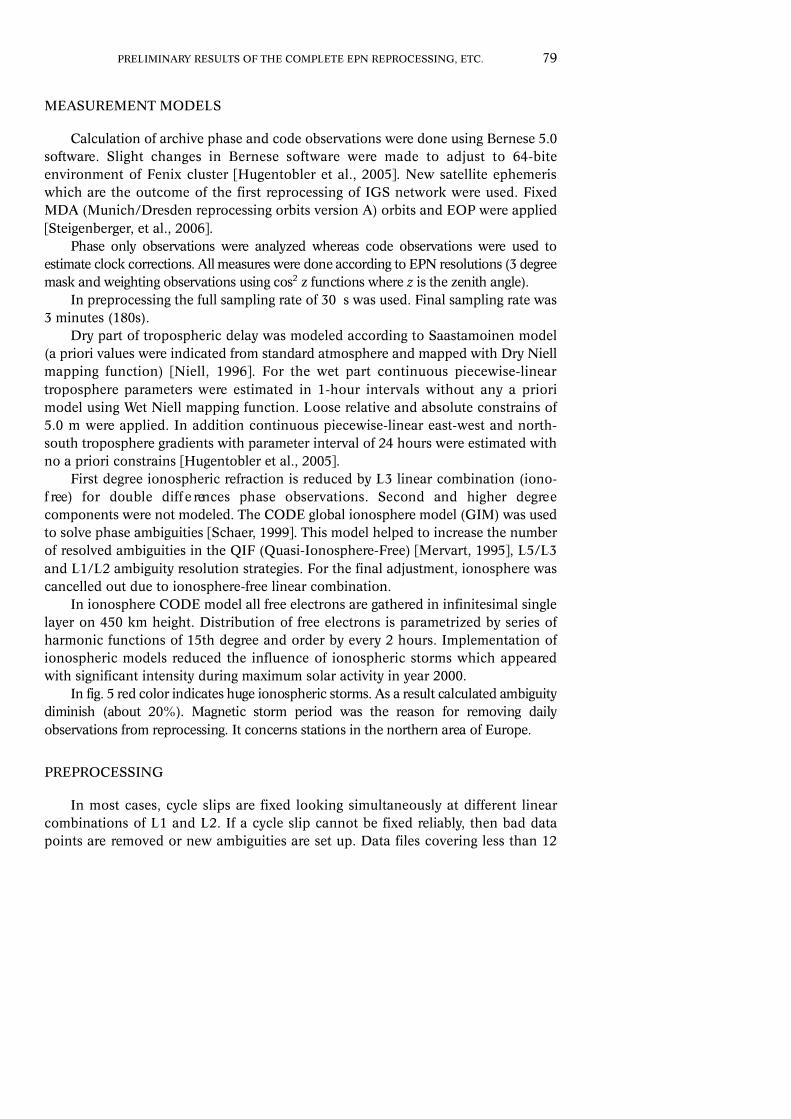
MEASUREMENT MODELS

Calculation of archive phase and code observations were done using Bernese 5.0software. Slight changes in Bernese software were made to adjust to 64-biteenvironment of Fenix cluster fHugentobler et al., 2005g. New satellite ephemeriswhich are the outcome of the first reprocessing of IGS network were used. FixedMDA (Munich/Dresden reprocessing orbits version A) orbits and EOP were appliedfSteigenberger, et al., 2006g.

Phase only observations were analyzed whereas code observations were used toestimate clock corrections. All measures were done according to EPN resolutions (3 degre emask and weighting observations using cos2 z functions where z is the zenith angle).

In preprocessing the full sampling rate of 30 s was used. Final sampling rate was 3 minutes (180s).

Dry part of tropospheric delay was modeled according to Saastamoinen model(a priori values were indicated from standard atmosphere and mapped with Dry Niellmapping function) fNiell, 1996g. For the wet part continuous piecewise-lineartroposphere parameters were estimated in 1-hour intervals without any a priorimodel using Wet Niell mapping function. Loose relative and absolute constrains of5.0 m were applied. In addition continuous piecewise-linear east-west and north-south troposphere gradients with parameter interval of 24 hours were estimated withno a priori constrains fHugentobler et al., 2005g.

First degree ionospheric refraction is reduced by L3 linear combination (iono-f ree) for double diff e rences phase observations. Second and higher degre ecomponents were not modeled. The CODE global ionosphere model (GIM) was usedto solve phase ambiguities fSchaer, 1999g. This model helped to increase the numberof resolved ambiguities in the QIF (Quasi-Ionosphere-Free) fMervart, 1995g, L5/L3and L1/L2 ambiguity resolution strategies. For the final adjustment, ionosphere wascancelled out due to ionosphere-free linear combination.

In ionosphere CODE model all free electrons are gathered in infinitesimal singlelayer on 450 km height. Distribution of free electrons is parametrized by series ofharmonic functions of 15th degree and order by every 2 hours. Implementation ofionospheric models reduced the influence of ionospheric storms which appearedwith significant intensity during maximum solar activity in year 2000.

In fig. 5 red color indicates huge ionospheric storms. As a result calculated ambiguitydiminish (about 20%). Magnetic storm period was the reason for removing dailyo b s e rvations from re p rocessing. It concerns stations in the nort h e rn area of Euro p e .

PREPROCESSING

In most cases, cycle slips are fixed looking simultaneously at different linearcombinations of L1 and L2. If a cycle slip cannot be fixed reliably, then bad datapoints are removed or new ambiguities are set up. Data files covering less than 12

PRELIMINARY RESULTS OF THE COMPLETE EPN REPROCESSING, ETC. 79

hours of data are automatically rejected. Posteriori normalized residuals of theobservations are checked for outliers, too. These observations are marked for thefinal parameter adjustment. Absolute antenna phase centre corrections based onIGS05 model considering antenna radome codes were used during calculations. Ifantenna/radome pair has no available calibrations, the corresponding values for theradome code «NONE» were used. Satellite antenna absolute phase centrecorrections were used based on IGS05 model.

QIF strategy was used to resolve ambiguities in a baseline processing mode usingCODE global ionosphere model (for baselines up to 2000 km length). For baselinelengths shorter than 100 km, L5/L3 approach was followed. For baselines shorterthan 10 km, L1/L2 approach was used. Fig. 4 shows resolved ambiguities acquiredaccording to presented method. Daily RINEX observation files containing less than50 percent of possible observation epochs were ignored. The two-step preprocessingmethod eliminated outliers (rejection criterion of L3 outliers: 0.0020 m; normalizedL1 zero-difference zenith value).

In addition the following models were customized:– planetary ephemeris DE405;– ocean tides OT_CSRC;– earth geopotential JGM3;– nutation IAU2000;– subdaily pole IERS2000;– tidal displacements (solid tides according to the IERS 1996/2000 standards);– ocean loading FES2004.

The datum of the daily and weekly solutions were defined by the MinimumConstraint (MC) approach applied for three Helmert translation parameters. The listof stations defining the datum included the following 14 IGS core stations: BOR1,BRUS, GRAS, HOFN, JOZE, METS, NYA1,ONSA, POLV, POTS, REYK, WSRT,WTZR, ZIMM fwww.epncb.oma.beg.

Fig. 4 – Ambiguity resolution rate of 1-day solutions. Blue - cumulative ambiguity resolution QIF+L5/L3+L1/L2.

80 M. FIGURSKI – P. KAMINSKI – A. KENYERES

Fig. 5 – Amount of calculated ambiguity processed by QIF method on the background of DST variation index(the DST index is an index of magnetic activity derived from a network of near-equatorial geomagnetic observ a t o r i e s ) .Circled green colour indicates period (1900s) when Selective Availability and Anty-Spoofing system was inactive.

PROCESSING SCHEME

The reprocessing was developed according to the newest standards used by EPNanalysis centres. All calculations were based on RINEX format standarized accordingto information received from IGS and EPN. Fig. 6 is a general scheme adopted inMUT to compute the calculations. EOP and MDA ephemeris in SP3 format from thefirst reprocessing of IGS elaborated by Steigenberger fSteigenberger, et al., 2006g

were used.Due to large number of re p rocessed stations, EPN network was fractioned

into subnetworks. Subnetworks were calculated on cluster computer as a parallelp rocess. Division into subnetworks was done by MKCLUS (Make Clusters)p rogramme. The division was automatic and included 50 to 60 stations.Minimum number of observations per satellite at each epoch value equal 3 wasi n t roduced into the MKCLUS programme. In the final process the subnetworksw e re joined in a group of re f e rence stations. For each subnetwork norm a lequation in Bernese format was generated. They were joined using ADDNEQ2p rogramme. Daily solutions were generated in SINEX format. At the same timestation coordinates and tropospheric parameters (Tro p o s p h e re Total ZenithDelay) were determ i n e d .

Daily and weekly time series of analyzed stations were obtained. Solutions werearchived on CAG servers. Fig. 7 shows an example of daily solutions of detrended(without constant and linear trend) ITRF 2005 cartesian coordinates before and afterthe reprocessing. The data concerns the same testing period.

PRELIMINARY RESULTS OF THE COMPLETE EPN REPROCESSING, ETC. 81

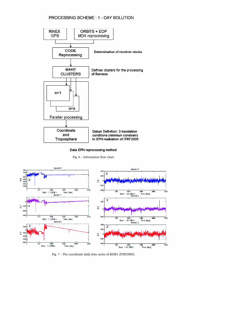
Fig. 6 – Information flow chart.

Fig. 7 – The coordinate daily time series of BOR1 (ITRF2005).

Reprocessing evidently improved the quality of the results on most of the EPNstations. Since trend and constant value were eliminated the dispersion and meanerror decreased.

However there are exceptions where re p rocessing did not bring anyimprovements in calculations. Despite reprocessing process very few stations havejumps and quite huge oscillation. HOFN (Hoefn, Iceland) station (fig. 8) is in theminority however.

Fig. 8 – The coordinate daily time series of HOFN (ITRF2005).

Fig. 9 – Wavelet symlet family.

PRELIMINARY RESULTS OF THE COMPLETE EPN REPROCESSING, ETC. 83

Based on daily reprocessing data we tried to detect station specific spectralcharacteristics in time series. Known tools to analyze frequency usually concernFourier transforms. To target the frequency of time series we chose the waveletanalysis tool. Wavelet based techniques gave the possibility of interpreting time andfrequency at the same time. More on wavelet overview can be found on the followingweb pages: http://www. a m a r a . c o m / c u rre n t / w a v e l e t . h t m l h t t p : / / c a s . e n s m p . f r / ~ c h a p l a i s /wavetour_presentation/Wavetour_presentation_US.html.

The Wavelet Toolbox is a collection of functions built on the MATLAB®Technical Computing Environment. It provides tools for the analysis and synthesis ofsignals and images, and tools for statistical applications as well.

Fig. 10 – The diagrams show exemplary ANKR station and its BLH series together with the results of H waveletanalysis and signal decomposition.

After several attempts to match wave type we decided to use symlet8. Thesymlets are nearly symmetrical wavelets proposed by Daubechies as modifications tothe db (Matlab’s shortcut) family. The best effects were obtained through 9th and

84 M. FIGURSKI – P. KAMINSKI – A. KENYERES

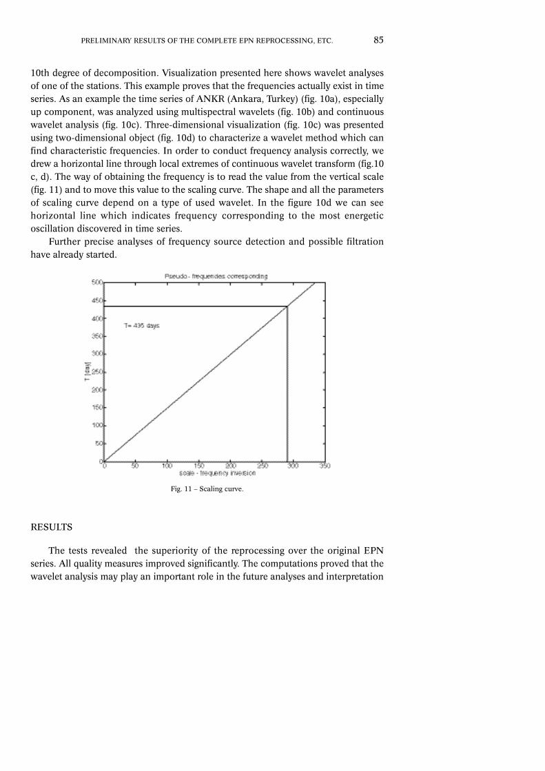
10th degree of decomposition. Visualization presented here shows wavelet analysesof one of the stations. This example proves that the frequencies actually exist in timeseries. As an example the time series of ANKR (Ankara, Turkey) (fig. 10a), especiallyup component, was analyzed using multispectral wavelets (fig. 10b) and continuouswavelet analysis (fig. 10c). Three-dimensional visualization (fig. 10c) was presentedusing two-dimensional object (fig. 10d) to characterize a wavelet method which canfind characteristic frequencies. In order to conduct frequency analysis correctly, wedrew a horizontal line through local extremes of continuous wavelet transform (fig.10c, d). The way of obtaining the frequency is to read the value from the vertical scale(fig. 11) and to move this value to the scaling curve. The shape and all the parametersof scaling curve depend on a type of used wavelet. In the figure 10d we can seehorizontal line which indicates frequency corresponding to the most energeticoscillation discovered in time series.

Further precise analyses of frequency source detection and possible filtrationhave already started.

Fig. 11 – Scaling curve.

RESULTS

The tests revealed the superiority of the reprocessing over the original EPNseries. All quality measures improved significantly. The computations proved that thewavelet analysis may play an important role in the future analyses and interpretation

PRELIMINARY RESULTS OF THE COMPLETE EPN REPROCESSING, ETC. 85

of EPN coordinate time series. We learned from the computations the following facts:available EPN database is not fully conforming with the current official EPNproducts. The database must be harmonized and checked. Final reprocessing shouldbe executed based on standard observations in RINEX format, corresponding withthe official names of EPN products (EPN SINEX file). RINEX format was modifiedand changed a few times since 1995. The changes were made in coding system ofreceivers and antennas in IGS as well. Until the start of the official re-processing allEPN antennas (current and historical) should have real absolute PCV modelavailable. The final reprocessing should be done following the IGS strategy in termsof the troposphere and ionosphere parameter estimation.

R E F E R E N C E S

Z. ALTAMIMI, P. SILLARD, C. BOUCHER (1994), CATREF software: Combination andanalysis of terrestrial reference frames. LAREG Technical Note SP08, InstitutGéographique National, France.

U. HUGENTOBLER, R. DACH, P. FRIDEZ (2005), Bernese GPS Software 5.0. Astron.Inst., Univ. of Berne, Berne, Switzerland. (Electronic version available athttp://www.bernese.unibe.ch/docs/ DOCU50.pdf).

A. KENYERES, J. LEGRAND, C. BRUYNINX, H. HABRICH, M. FIGURSKI (2008), Regionalre-analysis: Expectations and experiences within the EPN. IGS Workshop,Miami Beach, Florida, USA, 2-6 June.

L. MERVART (1995), Ambiguity resolution techniques in geodetic and geodynamicapplications of the Global Positioning System. Geod. Geophys. Arb. Schweiz,no. 53, p. 155.

A. NIELL (1996), Global mapping functions for the atmosphere delay at radiowavelengths. J. Geophys. Res., no. 101(B2), pp. 3227– 3246.

J. RAY, D. DONG, Z. ALTAMIMI (2004), IGS reference frames: status and futureimprovements. GPS Solutions, vol. 8(4), pp. 251-266, doi 10.1007/s10291-004-0110-x.

S. SCHAER (1999), Mapping and predicting the Earth’s ionosphere using the GlobalPositioniong System. Geod. Geophys. Arb. Schweiz, no. 59, p. 205.

P. STEIGENBERGER, M. ROTHACHER, R. DIETRICH, M. FRITSCHE, A. RÜLKE, S. VEY

(2006), Reprocessing of a global GPS network. Journal of GeophysicalResearch. vol. 111, B05402, doi 10.1029/2005JB003747.

86 M. FIGURSKI – P. KAMINSKI – A. KENYERES