PRELIMINARY REPORT ON AUTOMATED FRUIT

COUNTING FOR PHOTOGRAPHS

February 1974

Abstract

Although for a very specific case, the study demonstrates that

it is possible to develop a completely automated procedure for count-

ing oranges. This preliminary study shows that the most satisfactory

technique is one on which a count of the Number of Partial Oranges

seems to give the best agreement with the number of oranges counted

by photo interpreters. Using the multivariate discriminant procedure

in the Statistical Analysis System (SAS) and a formulated definition

of an orange, 100% correct classification was obtained for mature

oranges. The results for immature peaches were not as good as for

mature oranges. From the analysis it is apparent that film density

measurements on color Kodachrome slides based on the red filter con-

tribute significantly for automated fruit classification schemes.

Preliminary Report on Automated Fruit

Counting for Photographs

by

David V. Himmelberger

and

Ronald J. Steele

Contents

PageAbstract

HISTORY ••••••••••••••••••••••••••••.••••••••••••.••••••••• 1

Digitalization of Pictures •••••••••••••••••••••••

UNIVARIATE ANALYSIS

.....................................A •

I.

II.III.

Introduction

Classification

.................... .

...................................

3

3

5

8

IV. Analysis ............................•...•...•.... 11

v. Counting the Fruit .•.•.••••..•••.••.•.•.•••.•..... 17MULTIVARIATE ANALYSISB •

1. Introduction............. .

.....................................21

21

.................. .

Selection •••••••••••II .

III.

IV •

Sample

Procedures

Results

..............................................................

21

23

24

c. RECOl1MENDATIONS •••.••••••••••••••••••••••••••••••••••• 26

Bibliography

Appendix A

Appendix B

...............................................................................................................................

27

30

31

1

HISTORY

The problem of determining the total number of fruit on a tree has

long been of interest in crop estimation work. The first systematic

approach to this problem was described by Jessen [6] in 1955. Obviously,

a complete enumeration of fruit on a tree is quite an onerous and time

consuming task. Thus, in order to reduce the time and cost, Jessen pro-

posed a method of randomized branch sampling to obtain precise estimates

of the total number of fruit.

Over the past decade, the Research and Development Branch, Statisti-

cal Reporting Service (SRS), United States Department of Agriculture has

investigated various sampling techniques to estimate objective yields of

the following fruits and nuts: oranges [1,16,23], peaches [19,25], cher-

ries [10,14], apples [1,16,23], almonds [12]. pecans [24], walnuts [13],

filberts [8,21], grapefruit [1,16,23], and lemons [7]. In all the above

cases field crews counted fruit on selected limbs and the objective yield

estimate for a tree was then based on the reciprocal of the probability

of selection.

In March 1968, Huddleston first published a preliminary research

report [5] of earlier work begun in 1965 which examined the possibility

of using photography to increase sampling efficiencies. Trees without

leaves were photographed in an attempt to use the photograph as a sampling

frame for limb selection. In addition, photography was used to directly

obtain fruit counts of trees photographed on two sides using photo inter-

preters. However, realizing that accurate counting of fruit, even on a

sample basis, by field crews was a costly operation. Von Steen and Allen

[16) in 1969, and Allen in 1972 [1] further investigated the possibility

of using ground photography as an auxiliary information source to forecastyields of fruit.

2

A third approach to the problem of estimating the number of fruit on

a tree has been investigated by the Remote Sensing Group of the United

States Department of Agriculture. A small part of Allen's work in 1969-70

involved using aerial photography to make fruit counts [1]. This approach

cannot be considered significantly different from that of using ground

photography since human photo interpreters are relied upon for the fruitcounts in both cases.

In some earlier work by Von Steen, et al. [18], the relationship of

aerial photography reflectance to crop yields was investigated. They found

that when the optical density of the film was measured using red, green,

blue, and clear filters, the clear and red filters produced the highest

correlations when related to the yield indicators, but the magnitude of thecorrelation was too small to be useful in double sampling.

The newest method understudy for estimating yields of crops has encom-passed the domains of image processing, coding, transmission, and pattern

recognition as well as statistics and agriculture. The dramatic growth

of technology and interest in the environmental resources area has empha-

sized the potentialities for analyzing large quantities of data in the form

of pictures. In order to utilize the enormous collection of data, one must

be able to process it in both an efficient and expeditious manner.

All previous methods of counting fruit involved considerable time and

human energy. As the techniques advanced from the randomized branch sampling

to the photo interpretation, the human element was continually being reduced.

The current proposal is to retain all the elements of the estimator developed

using the photo counts, but to eliminate the photo interpreter. It is desira--,ble to eliminate the photo interpreter for several reasons. The first and

3

probably most important reason is that because the fruit counting task

is extremely monotonous and tedious, the accuracy of the counting varies

directly with time. Furthermore, the physical radiant energy of a scene

which is received by the photo interpreter will vary little from person

to person, however, it is individual perceptions of the physical stimuli

which interrelated physical and mental processes which will fluctuate

from person to person. No automated device can be expected to make the

complicated distinctions of which a human is capable, however, we can

expect the decision making process to be more consistant.

This report is broken into two Parts, A and B. Part A describes an

Univariate approach and Part B discusses a Multivariate approach.

PART A UNIVARIATE ANALYSIS

I. IntroductionPerhaps it is appropriate to briefly discuss what one could possibly

expect from a mathematical approach to the problem of counting fruit in

a picture. Bremermann [2] has estimated that even for a very coarse grid

(20 x 20) the number of variations of a prototype exceeds 1012, and this

number rapidly escalates to 1016 when one considers translations, rotations,

and dilations. Thus, at the present time, a table look-up solution is

technologically impossible. Instead, many simple tests can be applied

to reduce the number of configurations. Rather than attempting to develop

a model which encompasses every detail of the object to be identified, a

simpler approach is to isolate the essential features of the object and

eliminate all candidates which do not possess those properties. Theapproach is to apply a sequence of operations, each of which retains an

essential property. These operations may range from grey level filters

to test which measure area, convexity, and connectivity.

4

In most situations, one can assume that there are a finite number

of classes from which a pattern may have come, and each class can be

characterized by a probability distribution of the measurements. How-

ever, in some cases, it may not be pr.actical to specify the probability

distribution of the pattern classes, and in other cases the structure

of each class distribution may be known, but the parameters must be

estimated from training samples.

Before we proceed to the classification task, we must decide which

subset of the observed features is to be used as a set of features torepresent a pattern. The ability of an optimum classifier to discrimi-

nate given classes depends upon statistical separability measures between

class distributions in a given feature space. These measures then may

reflect the effectiveness of a feature set. It is known that the perfor-

mance of a pattern recognition system is closely related to the feature

measurements taken by the classifier. Fu [3] has presented some experi-

mental results for feature selection in multiclass pattern recognition

applied to a crop classification problem. From the experimental results,

one notes that it is possible for a feature subset to be almost as effec-

tive (in terms of percent recognition) as the complete feature set. Fu

points out that at present there is no unique feature selection technique

for all the possible pattern recognition problems. However, when class

distributions can be reasonably approximated by Gaussian distributions,

the parametric feature selection technique gives at least reasonable

evaluation of feature effectiveness.If one has complete freedom in the choice of features, they should

be chosen such that:

1. they separate the patterns,

5

2. their number is as small as possible, and

3. they minimize the probability of misclassification.

II. Digitalization of Pictures

The first phase of a computerized method of counting fruit is to

digitize the image. Since earlier research (16) on the use of aerial

photography had not indicated an appreciable gain in accuracy or cost

reduction over the ground photographs, it was decided to use the ground

photographs which photo interpreters had used to make their fruit counts.

This procedure involved taking a 35mm color photograph of the tree divided

into quadrants, one picture per quadrant, from a distance of about 20

feet. For a more precise explanation of the procedure, see the reference

"Use of Photography and Other Objective Yield Procedures for Citrus Fruit,"[16).

Using a Photometric Data Systems (PDS) Model 1014-0003 Microdensito-

merer System [9] each color transparency was digitized into an m x n array

of picture elements Xij, i - 1, •••,m and j = 1, •••, n, each of which was

quantified into one of 2k grey levels. Such an array would require m x n

k-bit words per picture to code any of the 2kmn possible pictures.

For this particular discussion, the entire 35mm transparency was

scanned into a 477x715 array of 212 - 4096 grey levels. Each picture

element, an analog to digital converted signal, is a 12 bit point trans-

mission recording. With a magnification of 50 X and circular aperture of

3.45mm in diameter, an effective aperture or spot size of 70 microns was

obtained. The scanning pattern was such that the distance between centerswas 50 microns in both the X and Y directions.

One must remember that we are viewing a two-dimensional projection

of a three-dimensional scene via a photograph, and the spectral properties of

6

the object of interest, the fruit, are greatly affected by the position

of the light source. The apparent distinct edge between the fruit and

the background tree which the photo interpreter observes is really a

shaded grey area when one more carefully inspects the transmission values

in a neighborhood of the apparent edge. This arises because of the spheri-

cal shape of the fruit and a point light source, the sun. Hence, a cir-

cular aperture was chosen because that shape more nearly approximated the

elliptical shape of the fruit than did the rectangular aperture.

The basic consideration in the choice of scanning pattern was to scan

the entire transparency as efficiently as possible while still retaining

the fixed effective circular aperture of 70 microns in diameter. This

requirement dictated the 50 micron distance between centers in both the

X and Y directions. The above pattern left only a small hole, approximately-3 2square 5xlO microns in area, in the center of an array of four transmis-

sion recordings (See Figure 1). It is not at all clear that the above

choice of filter size, magnification, and scanning pattern are optimum.

Since those questions were not a part of this project, no further attempt

will be made to discuss any optimality requirements. This area of the

problem is open to further research.

In order to span the visible portion of the spectrum, the same area of

the transparency was retraced three times. Each transparency was scanned

once with a clear, red, green, and blue Kodak filter. Unfortunately, due

to some tape handling problems, none of the transparencies in this discussion

had a complete set of four readings i.e., [X~ij - (clear, red, green, blue)].

Thus, rather than looking at this problem in a more general multivariatesetting, we shall restrict ourselves to a univariate analysis.

Figure I--Scanning pattern for an effective circular aperture of 70microns in diamete~. Shaded areas are exaggerated in thissketch.

7

8

III. Classification

An optimal classifier for this problem would be one that would

classify each transmission measurement into one of two classes, the

class of points which are fruit and those which are not fruit. One

could conceivably achieve this by using only one bit per picture ele-

ment. In any case, one would like to keep the number of classes as

small as possible because the computing time increases rapidly with

the number of classes.

In constructing a classification procedure, it is desirable to

minimize the probability of misclassification. That is, a good classi-

fication procedure is one which minimizes the cost of misclassification,

for a given confidence level. If one has some knowledge of his prior

probabilities, the underlying distributions of the classes, and the

costs of misclassification, then Bayes procedures give a method of

defining "minimum cost."

Let us now give a brief description of the classes among which we

wish to discriminate. First we must decide on the number of classes

into which we want to classify our data. We shall approach this ques-tion from an intuitive point of view. When the human observer looks

at Figure 2 there appear to be three distinct classes which have obviousspectral differences. From a gross perspective we shall identify each

class by describing the major components of the class.Class 1 is composed of the sky and dirt roadway. These areas are

usually the brightest portions of the picture.Class 2 will be our main class of interest, the fruit.

Class 3 the most popular class, is green leafy background and darkerportions of the scene.

9

Figure 2--An orange tree showing the three classes of spectral differencessky and roadways, fruit, and green leafy background.

10

Because the sample size of digitized transparencies was limited

and little was known about the distributions of the pattern classes,

it was decided to use a simple minded nonparametric classification pro-

cedure.

During the initial scanning of the picture, training information

was obtained. By scanning certain portions of the transparency which

were known to be members of the ith class, one was able to determine,

on a sample basis, the range and distribution of the three classes.

Thus, on the basis of grey level and training sample information above,

one would like to construct a classification procedure of the form:

and

oX-I

2

x e:; Class 1

if X e:; Class 2

X e:; Class 3,

(4.0)

X e:; Class 1 if Co < X = ClX e:; Class 2 if Cl < X = C2X £ Class 3 if Cz < X = C3, (4.1)

where the C's are positive real valued integers. The only difficulty

with the above procedure is that of estimating the constants Cj, j = 0,

1, 2, 3. Rather than having to estimate four constants as it might

appear, Co and C3 are lower and upper bounds respectively, which are

completely determined. The lower bound Co is zero because it is physi-

cally impossible to obtain a negative transmission measurement. The

upper bound (C3 = 4095) is fixed by the number of bits which are reserved

for each transmission recording. Hence, one need only estimate Cl and

C2 from the training samples. In our problem, Cl and C2 were equal to

52 and 140 respectively.

11

IV. Analysis

Once we have classified each transmission measurement according to

the grey level classification procedure, equation (4.0), we would like

to obtain an estimate of the probability of misc1assification. The

classification procedure adopted has no theretica1 basis upon which

we can make such an estimate, so we will give the empirically determined

misc1assification results for the orange tree shown in Figure 2. The

results presented in Table 1 will be only part of the total solution

of the problem of automatically counting the number of fruit from a trans-

parency because our object of interest, the 'orange', is a set of points.

TABLE 1

Point-by-Point classification summary by classes

Per Cent Number ofClass Correct Number of samples classified into class Samples

1 2 31 33.9 2431 2907 1842 71802 26.3 0 1179 3'309 4488-3 99.8 0 652 328735 329287

Total 97.4 2431 4738 333886 341055

The photo interpreter has a subjective mental image of an orange,

a leaf, a branch, sky, dirt, and how each of these objects differ from

one another. We must make the photo interpreter's perceptions of these

objects more precise, by defining them in mathematically quantifiable

terms, so that identification will no longer vary from interpreter to

interpreter.

In order to describe the class or set of points which constitute an

'orange', we shall look at the essential properties of the element of the

set.

12

That is, we must decide what we will accept as confirming evidence for

the statement, "A is an 'orange',11where A is a particular set of points.

The data which confirm a given hypothesis shall be restricted to mathema-

tically quantifiable terms. Our idea of confirmation should also satisfy

the equivalence condition. In Hempel's [4] terminology, an observation

report (data) which confirms a particular sentence (hypothesis) also con-

firms every sentence logically equivalent to that sentence.

We now propose the hypothesis H,

H: An 'orange' is a connected set of points (coded trans-mission values) of constant grey level with an ellip-tical boundary and major and minor axes of lengths Fand G, respectively.

Here "connected set,1I "elliptical boundary," "major axis," "minor axis,"

and "constant grey level" are terms of our quantifiable observational

vocabulary.

One should note that the observation reports upon which we are

relying are at two levels of introspection. The first level deals with

the elemental units, that is, the individual transmission values, and

the second level deals with properties and relations of certain sets of

the elemental units.

In the previous section on classification, we have already dealt

with the observation reports which look at the data point-by-point.

By using training samples on a classification procedure of the form of

equation (4.0), we have made a drastic reduction in the amount of data

which we will consider at our second and higher level of introspection.

(See Table 2)

<-

13

TABLE 2

Point-by-point Classification Results

Total Number of Points in Class

1 2 3(Fruit)

2431 4738 333886

We need only further consider those points which have the property

namely that of being a certain "constant grey level."

Property P: A point is said to have property P if itis the "constant grey level" correspond-ing to the transmission values in Class 2.

This observation report directly confirms hypothesis H.

Let us now proceed to those observation reports at the second

idea of confirmation that satisfies the equivalence relation, we know

that an observation report B disconfirms a hypothesis K if it confirms

the denial of K.Another property Q which supports the hypothesis H is the set

property of "connected set of points." Rather than look at the

observation report of "connected set of points" directly, we shall look

at its negation, which will provide disconfirming evidence for H. Thus,

we would like to eliminate from our domain of interest those points which

have property Q and do not have property P (symbolized QA ~P).

Property Q: A set of points possesses Property Q if itcontains horizontal runs less than lengththree or vertical runs less than length two.

14

This will eliminate all singles in the vertical direction and all singles1./

and doubles in the horizontal direction which have property P. Thosesets of points not eliminated Le., those possessing Properties P •...•Q are

"connected sets of points."A more sophisticated approach to the property of "connected set of"points is that given by Wilkins and Wintz [22]. They describe a contour

tracing algorithm (CTA) which locates and traces all contours of any 2-

dimensional data array. The algorithm first finds an initial or ~tarting

point and then traces the outer boundary of the largest connected set of

elements having the same grey level as the initial point, always terminat-

ing at the initial point.One could also think of defining some statistic which would give a

measure of, say, the eccentricity of the contour. These techniques should

give better results than our simple idea of using runs. However, due to

the time involved in programming the CTA, we have postponed using those

techniques until a later date.

One of the difficulties with the automated approach to the problem

of counting fruit is that of keeping the notion of an 'orange' flexible

enough to pick out a rather wide class of objects which satisfy the pro-

perties of an orange, but rigid enough to give consistent results. This

difficulty is further complicated by the fact that many of the fruit one

sees in a photograph are either partically camouflaged or else appears in

clusters.

1/ In any ordered sequence of elements of two kinds, each maximal

subsequence of elements of like kind is called a run. For example, the

sequence a:cr:cr: S a:cr: 8SS a: opens with an alpha run of length 3; it is followedby runs of length 1, 2, 3, 1, respectively.

--

15

By eliminating runs of length one and two, we have decided not to attempt

to count the very small parts of an orange which might be visible between

the leaves and branches. The separate reductions for elimination of

horizontal and vertical runs are given in Table 3.

TABLE 3

Data Reduction by Eliminating Short Runs in Class 2

Total Number Number of Points in Number of Points Number of Pointsof Points Horizontal Runs of in Vertical Runs Not Eliminated

Length 1 and 2 of Length 1Eliminated Eliminated

4738 1342 1297 2099

The reduction given in Table 3 have been obtained by first e1imi-

nating horizontal runs and then vertical runs. This operation is

definitely not commutative. Furthermore, one may wish to apply the run

elimination procedure repeatedly until the data reduction terminates.

Since we are only interested in the set of points which are elements

of Class 2, the fruit, and the set of points which are not fruit, we actually

have a two class classification problem. One should note that after the

short runs are removed from Class 2, they are then classified into the com-

pliment of that set. The classification summary for the reduced two class

problem after run removal is presented below in Table 4.

16

TABLE 4

Classification Summary After Run Removal

Per Cent Number ofClass Correct Number of Points Classified As Samples

Fruit Non Fruit

Fruit 25.0 1122 3366 4488

Non Fruit 99.7 977 335590 336567

Total 98.7 2099 338956 341055One can readily construct examples to prove the noncommutativity

of the operation of run elimination on opposite directions for two

dimensional arrays. Suppose we let h symbolize elimination of runs of

length one and two in the horizontal direction, and v symbolize e1imi-

nation of runs of length one in the vertical direction.

We wish to prove the following:

Theorem I: hv ~ vh

Proof: Let us assume the above relation does hold. Consider the following

array in which we let a "2" represent a point belonging to Class

2, an "x" represent a point not in Class 2, and a

a point removed by run elimination.

"_" represent

2 2 2 x 2 2 2

222 2 2 x x

2 2 2 x 2 2 2

/::::::: v

2 2 2 x 2

)222-2xx

x - - x x x x

x 2 2 x x x x

2 2 2 x 2

2 2 2 - 2 x xx 2 2 x x x x

h

2 2 2 x -l222--xx

x--xxx.

--

17

It is obvious that the resulting two dimensional arrays are not equi-

valent. Q.E.D.One may note in the above counterexample that by again eliminating

runs in the sequence hv, we can obtain still further reduction to

2 2 2 x.

2 2 2 - - x x

x - - x x x x

which is equivalent to vh.

A more general theorem is stated in Appendix A without proof.

The property of the set having an "elliptical boundaryll is partially

included in our formulation of Property A -Q and in our counting method

which is described later. Thus we will not isolate the property of an

"elliptical boundary," but rather will incorporate it in the observation

reports of the run property and size property.

To this point, we have narrowed our domain of interest to only

those sets of points which have properties P and not Q (symbolized

pA -Q). We now wish to devise an algorithm which will count the number

of objects, 'oranges', which have the size property S, IImajor axis oflength eight,1l and "minor axis of length six."

Property S: A nonempty set of points is said to haveProperty S if it is a "connected set ofpoints" with area 1r FG/4, where F and Gare the lengths of the major and minoraxes.

V. Counting the Fruit

Although the final phase of accepting or rejecting the hypothesis

H could be construed as pragmatic, we wish to establish general IIrules

of acceptance." [4] These rules would formulate fixed criteria which

determine the acceptance or rejection of the hypothesis by evaluating

the amount of confirming or disconfirming evidence in the accepted obser-vation reports.

18

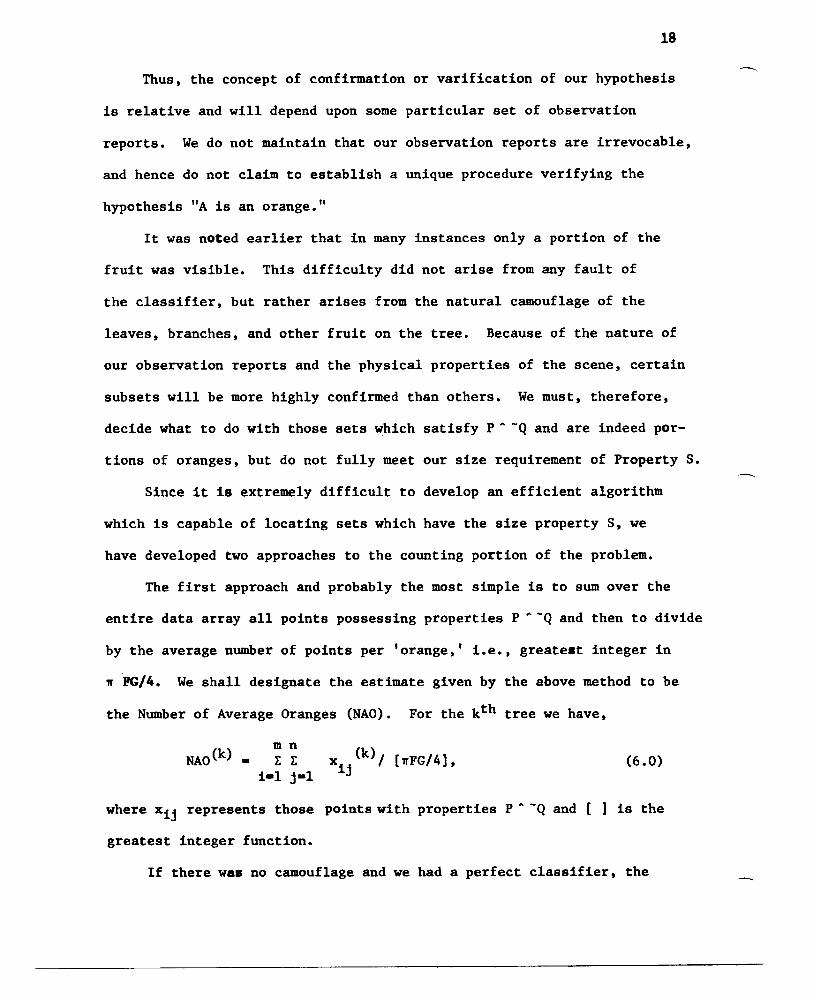
Thus, the concept of confirmation or varification of our hypothesis

is relative and will depend upon some particular set of observation

reports. We do not maintain that our observation reports are irrevocable,

and hence do not claim to establish a unique procedure verifying the

hypothesis "A is an orange."

It was noted earlier that in many instances only a portion of the

fruit was visible. This difficulty did not arise from any fault of

the classifier, but rather arises from the natural camouflage of the

leaves, branches, and other fruit on the tree. Because of the nature of

our observation reports and the physical properties of the scene, certain

subsets will be more highly confirmed than others. We must, therefore,

decide what to do with those sets which satisfy pA -Q and are indeed por-

tions of oranges, but do not fully meet our size requirement of Property S.

Since it is extremely difficult to develop an efficient algorithm

which is capable of locating sets which have the size property S, we

have developed two approaches to the counting portion of the problem.

The first approach and probably the most simple is to sum over theentire data array all points possessing properties P A_Q and then to divide

by the average number of points per 'orange,' i.e., greatest integer in

'lrPG/4. We shall designate the estimate given by the above method to be

the Number of Average Oranges (NAO). For the kth tree we have,

NAO(k) _ xij

(k) / ['lrFG/4], (6.0)

where Xij represents those points with properties P A -Q and [ ] is the

greatest integer function.

If there was no camouflage and we had a perfect classifier, the

(6.1)

19

Average Orange (AO) approach would give us an unbasied estimate. How-

ever, the AO approach makes little use of the fact that we have several

classes of oranges we are attempting to count.The three basic classes of oranges we shall consider are:

(i) a whole single orange,

(ii) a cluster of oranges, and

(iii) a partial orange.

Case (i) presents no problems, but in cases (ii) and (iii) where only

partial fruit are visible the NAO may grossly underestimate the true

number of oranges. For instance, if seven partial fruit have an area

equivalent to one Average Orange, we would have an undercount of six.

The motivation behind the second counting approach was to develop

a simple algorithm which would search the entire data array and count

partial oranges. The algorithm partitions the data matrix into" boxes"

which are arrays of dimension ten rows by ten columns and checks each

"box" according to the Partial Orange criterion given in equation (6.1)

We obtain the Number of Partial Oranges (NPO)1 in the 1th "box" as,10 10

NPOI - L L Xijl / [wFG/l2],i-I j-l

and the Number of Partial Oranges (NPO)k on the kth tree as the sum of

the Number of Partial Oranges over all 1 "boxes,"NPO(k)_ ENPO (k)

1 1(6.2)

One readily observed from equation (6.1) that a Partial Orange is about

one-third an Average Orange. Although the NPO approach has its short-

comings, it does represent an attempt to utilize the clustering property

of sets of points substituting an 'orange.'

The estimates for the Number of Average Oranges, equation (6.0),

Number of Partial Oranges, equation (6.2), and the photo interpreter

20

counts for the orange tree shown in Figure 2 are presented in Table 5.

TABLE 5

Number of oranges in lower right quadrant of Figure 2 as determinedby three different counting methods.

Number of Number of Number of OrangesCounted by

Average Oranges Partial Oranges Photo Interpreters

57 85 74

21

PART B MULTIVARIATE ANALYSIS

I. Introduction

Results from preliminary investigations using the discriminant

analysis procedure in SAS have been very encouraging. The classifica-

tion criterion was determined by a measure of generalized square distance.

Three groups were used and the distance measure was based on the indivi-

dual within-group covariance matrices since they were significantly

different at the 0.001 level. The three groups which were used were

sky, background (foilage, tree, etc.), and fruit. These groups were

used since, when the entire photographs were scanned, small areas were

also scanned which contained only background, sky, or fruit. These

small scan areas were rectangular, so when fruit were scanned, some

background points were included. SAS data sets were formed from each of

these small scan areas and were stored on tape. However, in order for

SAS to access these data sets, they had to be moved back to disk.

II. Sample Selection

Input to the discriminant procedure required a minimum of two obser-

vations per group for calibration data to form the within-group covariance

matrices in order to develop the classification criteria. However, at

least ten observations should be used to obtain a good classification

criterion. Since the transmission values are fairly homogeneous

each group, systematic sampling was used for selection of calibration

data for sky and background. Realizing, of course, that a systematic

sample yields a biased estimate of the covariance matrix. As mentioned

earlier, when the small areas containing fruit were scanned, some back-

ground points were included in the rectangular area. In order tomake

sure the calibration data for fruit was actually fruit, two different

24

may be that two filters would yield good enough classification results

for counting fruit, thus reducing the amount of scanning and data to

handle.

IV. Results

These initial results should not be viewed as conclusive, however,

there have been several findings which appear quite promising and should

be explored further. On orange trees with ripe fruit, it appears there

are no substantial differences in classification results between using

1) all four filters, 2) the clear, red, and blue filters, or 3) the red,

green, and blue filters. Using our definition of "correct" classification,

all the above combinations yielded 100% "correct" classification. The

three filter combinations classified more than 99% of the data points

into the same groups. Thus, although there were a few discrepencies on

a point-by-point basis, they were nominal. Table 5 shows how many points

were classified into each group by the various filter combinations on a

slide-by-slide basis for both oranges and peaches.

In Appendix B, Tables 6-53 contain the simple statistics; the

variance and covariance matrices and the pairwise squared distance between

groups for each of the filter combinations listed in Table 6. It can be

seen from these tables that the mean vectors of the groups are quite

different. The method of grouping did an excellent job of separating

the data points for all four trees. However, the limitation of this

approach is the fact that one does not know the exact origin of each data

point. If the formulated definitions were correct, the multivariate tech-

nique shows a promising approach to automated fruit counting.

25

TABLE 5

Point-by-point classification results by

slide, by type, by dass, and by filter combination

Slide Type Filters Foi1age Fruit Sky

Orange CRGB 622 222 50

A Orange CRB 623 220 51Orange RGB 620 224 50

Orange CRGB 582 260 52

B Orange CRB 574 268 52Orange RGB 576 268 50

Peach CRGB 328 287 51Peach' CRB 332 282 52

C Peach RGB 346 272 48Peach CGB 358 256 52

Peach CRG 338 277 51

Peach CRGB 348 230 286Peach CRB 369 213 282

D Peach CRG 376 202 286Peach CGB 315 271 278Peach RGB 356 213 286

The results for peaches are not as good as for oranges. The filter combi-

nations containing the red filter showed nearly the same classification

re6u1ts with less than 2% of the points being classified into different

26

groups. However, when the red filter was omitted, the classification

results changes substantially, as can be seen from the previoustable. Thus, it appears the red filter makes a substantial contribution

for classification of peaches.

c. RecommendationsThis study points out the need for further research in the following

areas:

1. A test needs to be conducted using known fruit and various back-

grounds particularly with the multivariate approach. That is, a

sample of known fruit and backgrounds should be scanned. Then

a sub-sample of these could be used as training and the remainder

used in the test. This would permit one to evaluate how well

one can classify fruit.

2. Determine the optimum magnification level, aperture size, and

shape, and sampling interval for scanning.

3. Compare the results from the parametric multivariate classifica-

tion model with a non-parametric classification model, for a

suitable number of samples.

4. Tests should be made to determine if the mean vectors and covariance

matrices are significantly different between fruit within each

tree and between trees within the sameimaturity category.

5. Develop a sophisticated contour tracing algorithm which is capa-

ble of counting connected sets of points.

6. Develop an automated fruit counting system which could support an

operational program both time and cost-wise •.-

27Bibliography

[1] Allen, R. D., "Evaluation of Procedures for Estimating Citrus Fruit

Yield," R&D, SRS, USDA, February 1972.

[2] Bremmerman, H. J., "What Mathematics Can and Cannot Do for Pattern

Recognition, IIBerkeley, California.[3] Fu, K. S., and Min, P. J., "On Feature Selection in Multiclass Pat-

tern Recognition," Technical Report Number TR-EE68-11, School

of Electrical Engineering, Purdue University, July 1968.

[4] Hempel, C. G., "Studies in the Logic of Confirmation," Aspects of

Scientific Explanation, New York, The Free Press, (1966).

[5] Huddleston, H. F., "The Use of Photography in Sampling for Objective

Yields of Deciduous Fruits," R&D, Statistical Reporting Service,

U.S. Department of Agriculture, Washington, D.C., March 1968.[6] Jessen, R. J., "Determining the Fruit Count on a Tree by Randomized

Branch Sampling,1I Biometrics, March 1955.

[7] Kitterman, J. M.; Johnson, Doyle, C. and Henderson Lemon Crop Fore-

casting Project, February 1971 Survey; California Crop and Live-

stock Reporting Service, March 10, 1971.

[8] Lautenschlager, Lyle F., "Evaluation of New Filbert Objective Yield

Procedures, R&D, SRS, USDA, January 1972.

[9] Photometric Data Systems Corporation, Bulletin No. 636, 841 Holt

Road, Webster, N.Y. 14580, (1970).

[10] Small, Richard P., "Research Report on Tart Objective Yield Surveys,"

R&D, SRS, USDA, December 1967.

[111 Sturdevant, Tyler R., "Research Report on Virginia Apple Objective

Count Surveys~ R&D, SRS, USDA, October 1967.

28

[12) Swedberg, J. H., Johnson Doyle C., and Henderson W. Ward, "Almond

Objective Measurement Forecasting Research Project," California

Crop and Livestock Reporting Service, July 20, 1972.

[13) Swedberg, J. H., Johnson, Doyle C., and Henderson, W. Ward. "Walnut

Objective Measurement Forecasting Research Project," California

Crop and Livestock Reporting Service, September 15, 1972.

[14) Vogel, Fred A., "A Research Report on Michigan Tart Cherries, R&D, SRS,

USDA, April 1970.

[15] Vogel, Fred A., "A Technical Note on PPS Sampling with an Application

to Fruit and Nuts," R&D, SRS, USDA, March 1970.

[16] Von Steen, D. H.,-and Allen, R. D., "Use of Photography and Other

Objective Yield Procedures for Citrus Fruit," Research and Deve-

lopm~nt Branch, Statistical Reporting Service, U.S. Department

of Agriculture, Washington, D.C., June 1969.

[17] Von Steen, D. H., Hurt, P., and Allen, R. D., "Remote Sensing Relation-

ship of Aerial Photography Reflectance to Crop Yields," R&D, SRS,

USDA, June 1969.[18] Von Steen, D. H., Leamer, R. W., and Gerbermann, A. H., "Relationship

of Film Optical Density to Yield Indicators," R&D, SRS, USDA, and

Southern Plains Branch, Soil and Water Conversation Research Divi-

sion, Agriculture Research Service of the USDA.

[19] Warren, Fred B., and Wigton, William H., "Sampling for Objective Yields

of Apples and Peaches, Virginia 1969, R&D, SRS, USDA, February 1973.

[20) Wigton, William H., and Kibler, William E., "New Methods for Filbert

Objective Yield Estimation," Agricultural Economics Research, Vol.

24, No.2, April 1972.

29

[21] Wilkins, L. C., and Wintz, P. A., "Studies on Data Compression, Part I:

Picture Coding By Contours," TR-EE70-l7, School of Electrical

Engineering, Purdue University, September 1970.

[22] Williams, S. R., "Forecasting Florida Citrus Production - Methodology

and Development, Florida Crop and Livestock Reporting Service,

January 1971.

[23] Wood, Ronald A., "A Study of the Characteristics of the Pecan Tree

For Use in Objective Yield Forecasts, R&D, SRS, USDA, 1971.

[24] Wood, Ronald A., and Warren, Fred B., "A Study of Sampling and Estimat-

ing Procedures for California Cling Peaches, R&D, SRS, USDA, Jan-uary 1972.

30

Appendix A

Theorem II: For any finite two dimensional real array A - (aij), if

one successively applies the operation of eliminating runs less than

length p in the horizontal direction, then eliminating runs less than

length q in the vertical direction, and continues to alternate operat-

ing on the rows and columns until no further elimination is possible,

then the resultant array H • (hij) is equivalent, in the sense that the

elements not eliminated are in the same positions for all aij, to the

array V = (vij) where V was obtained by first operating on the columns

and then on the rows and so on until data reduction terminated. Further-

more, the smallest subset which will not be eliminated is of dimension

(p + 1) X (q + 1).

Appendix B

Tables 6 - 53

31

32

Table 6--Simp1e statistics for orange tree A: Four variables - clear,red, green, and blue.

Bac.kgroundStandard

Variable N Sum Mean Variance Deviation

Clear 38 12878.00 338.89 35058.09 187.23

Red 38 21584.00 568.00 53741.18 231. 82

Green 38 16012.00 421. 36 42642.40 206.50

Blue 38 18580.00 488.94 48269.34 219.70

-----------------------------------------------------------------------Fruit

Clear 16 3300.00 206.25 738.60 27.17

Red 16 3142.00 196.37 505.11 22.48

Green 16 3690.00 230.62 715.05 26.74

Blue 16 8386.00 524.12 3531. 45 59.42

-----------------------------------------------------------------------Sky

Clear 10 310.00 31. 00 39.33 6.27

Red 10 650.00 65.00 255.33 15.97Green 10 774.00 77 •40 127.15 11. 27

Blue 10 900.00 90.00 136.88 11. 69

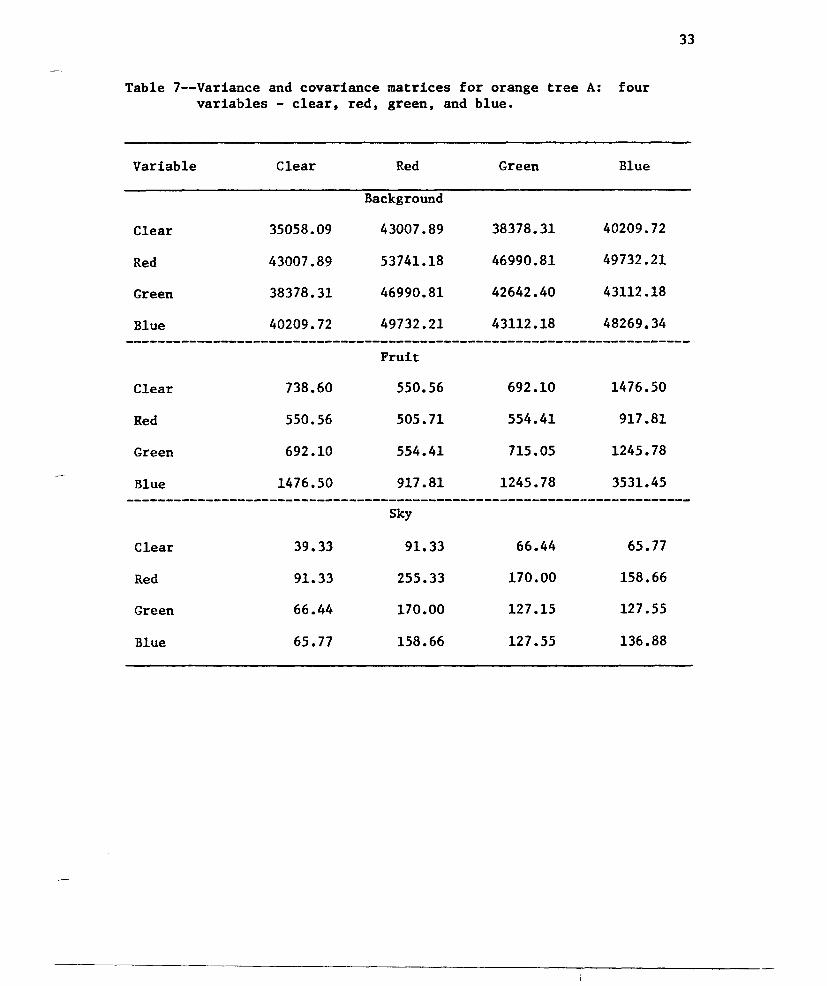
Table 7--Variance and covariance matrices for orange tree A: fourvariables - clear, red, green, and blue.

33

Variable Clear Red Green Blue

Background

Clear 35058.09 43007.89 38378.31 40209.72

Red 43007.89 53741.18 46990.81 49732.21

Green 38378.31 46990.81 42642.40 43112.18

Blue 40209.72 49732.21 43112.18 48269.34-----------------------------------------------------------------------Fruit

Clear 738.60 550.56 692.10 1476.50

Red 550.56 505 •71 554.41 917.81

Green 692.10 554.41 715.05 1245.78

Blue 1476.50 917.81 1245.78 3531.45-----------------------------------------------------------------------Sky

Clear 39.33 91. 33 66.44 65 •77

Red 91. 33 255.33 170.00 158.66

Green 66.44 170.00 127.15 127.55

Blue 65.77 158.66 127.55 136 •88

34

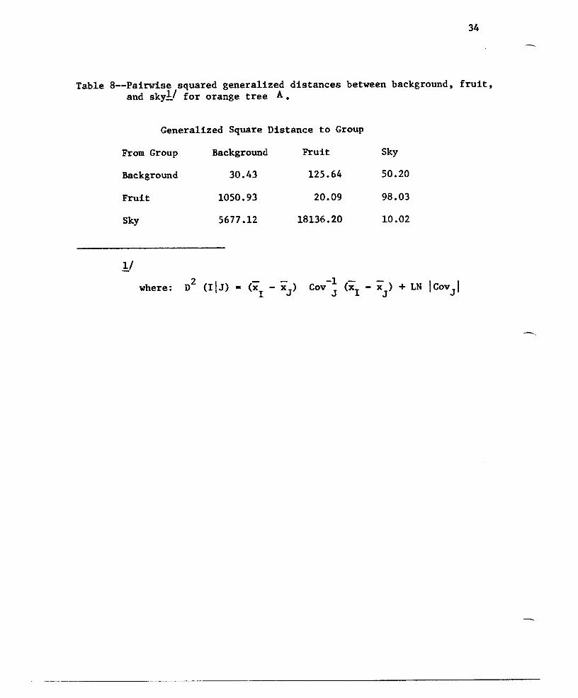
Table 8--Pairwise squared generalized distances between background, fruit,and sky11 for orange tree A.

Generalized Square Distance to Group

From Group

Background

Fruit

Sky

Background

30.43

1050.93

5677 .12

Fruit

125.64

20.09

18136.20

Sky

50.20

98.03

10.02

!/where: D

2 (IIJ) = (x - x )I J

35

Table 9--Simp1e statistics for orange tree A: Three variables - clear,red, and blue.

Variables N Sum Mean Variance StandardDeviation

Background

Clear 38 12878.00 338.89 35058.09 187.23

Red 38 21584.00 568.00 53741.18 231. 82

Blue 38 18580.00 488.94 48269.34 219.70-----------------------------------------------------------------------Fruit

Clear 16 3300.00 206.25 738.60 27.17

Red 16 3142.00 196.37 505.71 22.48

Blue 16 8386.00 524.12 3531. 45 59.42-----------------------------------------------------------------------Sky

Clear 10 310.00 31.00 39.33 6.27

Red 10 650.00 65.00 255.33 15.97

Blue 10 900.00 90.00 136 •88 11.69

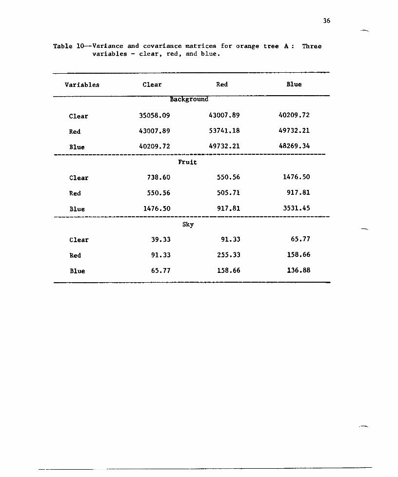
36

Table 10--Variance and covariance matrices for orange tree A: Threevariables - clear, red, and blue.

Variables ClearBackground

Red Blue

Clear

Red

Blue

35058.09

43007.89

40209.72

43007.89

53741.18

49732.21

40209.72

49732.21

48269.34----------------------------------------------------------------------Fruit

Clear

Red

Blue

Clear

Red

Blue

738 •60

550.56

1476.50

39.33

91. 33

65.77

Sky

550.56

505.71

917 .81

91. 33

255.33

158.66

1476.50

917 •81

3531.45

65.77

158.66

136.88

37

Table 11--Pairwise squared generalized distances between'background, fruit,and sky!.! for orange tree A:

Generalized Squared Distance to Group

From Group

Background

Fruit

Sky

Background24.94

1037.30

3748.96

Fruit

107.63

16.59

3773.38

Sky43.67

89.85

10.70

1/ where:

38

Table 12--Simp1e statistics for orange tree A: Three variables - red,green, and blue.

Variable N Sum Mean Variance StandardDeviation

Background

Red 38 21584.00 568.00 53741.18 231.82

Green 38 16012.00 421.36 42642.40 206.50

Blue 38 18580.00 488.94 48269.34 219.70-----------------------------------------------------------------------Fruit

Red 16 3142.00 196.37 505.71 22.48

Green 16 3690.00 230.62 715 .05 26.74

Blue 16 8386.00 524.12 3531.45 59.42-----------------------------------------------------------------------Sky

Red 10 650.00 65.00 255.33 15.97

Green 10 774 •00 77 .40 127.15 11. 27

Blue 10 900.00 90.00 136.88 11.69

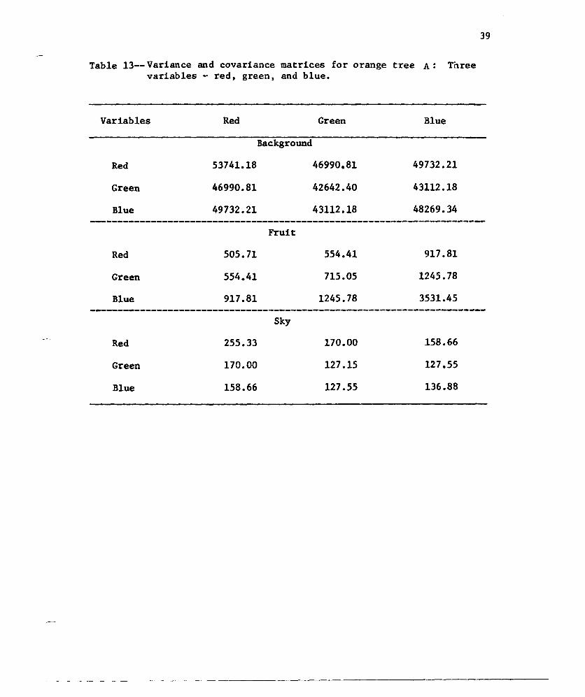
Table 13-- Variance and covariance matrices for orange tree A: Threevariables - red, greent and blue.

39

Variables Red

Background

Green Blue

Red

Green

Blue

Red

Green

Blue

Red

Green

Blue

53741.18

46990.81

49732.21

505.71

554.41

917.81

255.33

170.00

158.66

Fruit

Sky

46990.81

42642.40

43112.18

554.41

715 .05

1245.78

170.00

127.15

127.55

49732.21

43112.18

48269.34

917.81

1245.78

3531.45

158.66

127.55

136.88

40

Table 14--Pairwise squared generalized distances between background, fruit,and sky11 for orange tree A :

Generalized Squared Distance to Group

From Group

Background

Fruit

Sky

Background

25.91

767.172337.14

Fruit

118.49

18.09

16281.54

Sky

40.25

76.06

9.54

!Iwhere:

41Table 15--Simp1e statistics for orange tree B: Four variables - red,

green, blue, and clear.

Variable N Sum Mean Variance StandardDeviation

Background

Red 32 18694.00 584.18 46314.93 215.20

Green 32 15358.00 479.93 40154.44 200.38

Blue 32 18412.00 575.37 42647.59 206.51

Clear 32 12990.00 405.93 34587.99 185.97-----------------------------------------------------------------------Fruit

Red 16 1728.00 108.00 786.66 28.04

Green 16 3448.00 215.50 1254.66 35.42

Blue 16 6946.00 434.12 2525.58 50.25

Clear 16 3020.00 188.75 1096.46 33.11-----------------------------------------------------------------------Sky

Red 10 650.00 65.00 255.33 15.97

Green 10 774 •00 77 .40 127.15 11.27

Blue 10 900.00 90.00 136.88 11.69

Clear 10 310.00 31.00 39.33 6.27

Table 16--Variance and covariance matrices for orange tree B: Fourvariables - red, green, blue, and clear.

42

Variable Red Green Blue Clear

BackgroundRed 46314.93 42816.14 43386.95 39776.91

Green 42816.14 40154.44 40282.28 37084.64

Blue 43386.95 40282.28 42647.59 38092.50

Clear 39776.91 37084.64 38029.50 34587.99-----------------------------------------------------------------------Fruit

Red 786.66 909.60 1188.26 847.20

Green 909.60 1254.66 1580.60 1151. 60

Blue 1188.26 1580.60 2525.58 1582.03

Clear 847.20 1151. 60 1582.03 1096.46-----------------------------------------------------------------------Sky

Red 255.33 170.00 158.66 91. 33

Green 170.00 127.15 127.55 66.44

Blue 158.66 127.55 136.88 65.77

Clear 91.33 66.44 65.77 39.33

.-

43

Table 17--Pairwise squared generalized distances between background, fruit,and sky11 for orange tree B.

Generalized Squared Distance to Group

From Group Background Fruit

Background 27.82 122.61

Fruit 910.05 20.20

Sky 8734.00 8209.17

Sky

100.75

142.96

11.02

11

where:

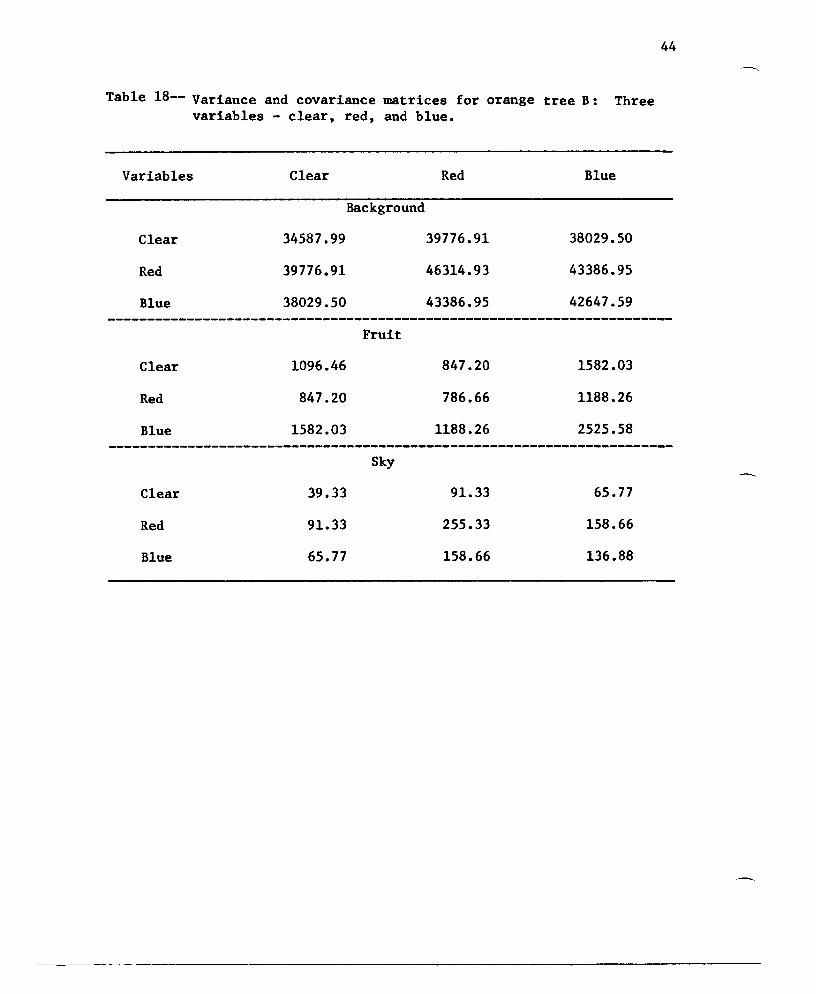
Table 18-- Variance and covariance matrices for orange tree B: Threevariables - clear, red, and blue.

44

Variables

Clear

Red

Blue

Clear

Red

Blue

Clear

Red

Blue

Clear

Background

34587.99

39776.91

38029.50

Fruit

1096.46

847.20

1582.03

Sky

39.33

91.33

65.77

Red

39776.91

46314.93

43386.95

847.20

786.66

1188.26

91.33

255.33

158.66

Blue

38029.50

43386.95

42647.59

1582.03

1188.26

2525.58

65.77

158.66

136.88

45

Table 19--Simp1e statistics for orange tree B: Three variables - clear,red, and blue.

Variable N Sum Mean Variance StandardDeviation

Background

Clear 32 12990.00 405.93 34587.99 185.97

Red 32 18694.00 584.18 46314.93 215.20

Blue 32 18412.00 575.37 42647.59 206.51-----------------------------------------------------------------------Fruit

Clear 16 3020.00 188.75 1096.46 33.11

Red 16 1728.00 10B.00 786.66 2B.04

Blue 16 6946.00 434.12 2525.58 50.25-----------------------------------------------------------------------Sky

Clear 10 310.00 31.00 39.33 6.27

Red 10 650.00 65.00 255.33 15.97

Blue 10 900.00 90.00 136. 88 11.69

46

Table 20--Pairwise squared generalized distances between background, fruit,and skyl! for orange tree B •

Generalized Squared Distance to Group

From Group

Background

Fruit

Sky

1/

Background

23.23

816.93

6775.07

Fruit

117 •05

17.33

3655.53

Sky

66.69

126.63

10.70

47

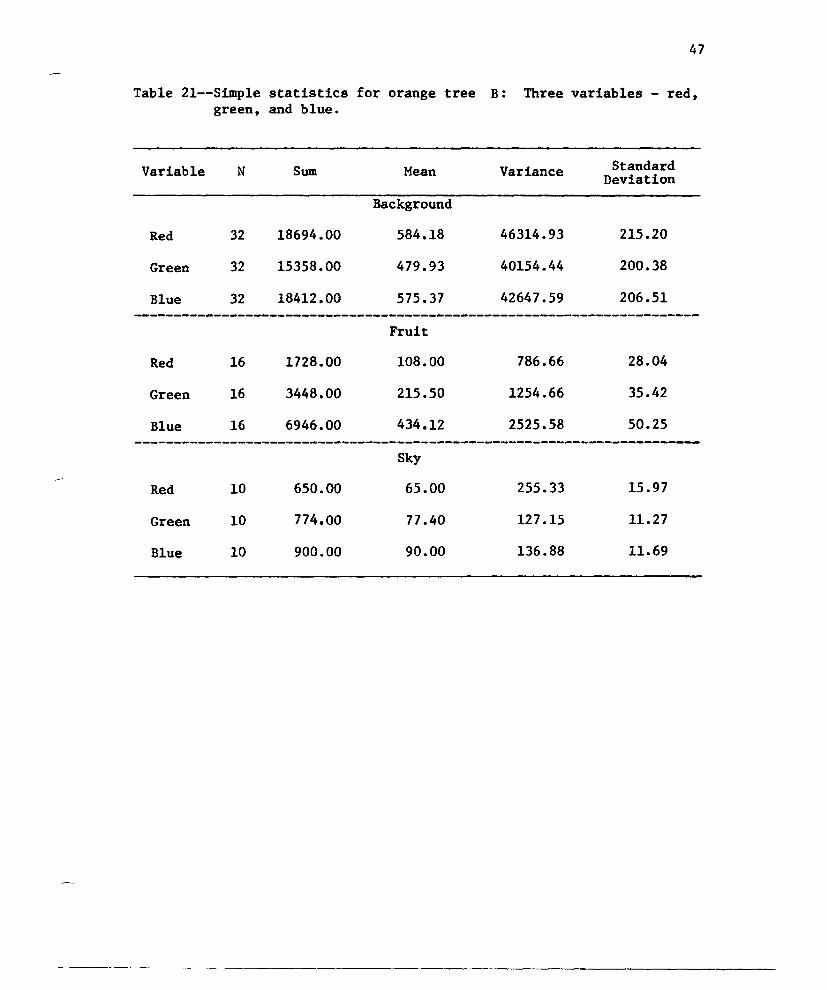
Table 21--Simp1e statistics for orange tree B: Three variables - red,green, and blue.

Variable N Sum Mean Variance StandardDeviation

Background

Red 32 18694.00 584.18 46314.93 215.20

Green 32 15358.00 479.93 40154.44 200.38

Blue 32 18412.00 575.37 42647.59 206.51-----------------------------------------------------------------------Fruit

Red 16 1728.00 108.00 786.66 28.04

Green 16 3448.00 215.50 1254.66 35.42

Blue 16 6946.00 434.12 2525.58 50.25-----------------------------------------------------------------------Sky

Red 10 650.00 65.00 255.33 15.97

Green 10 774.00 77 •40 127.15 11.27

Blue 10 900.00 90.00 136 •88 11.69

Table 22-- Variance and covariance matrices for orange tree Bvariables - red, green, and blue.

Three

48

Variables RedBackground

Green Blue

Red

Greed

Blue

46314.93

42816.14

43386.95

42816.14

40154.44

40282.28

43386.95

40282.28

42647.59-----------------------------------------------------------------------Fruit

Red

Green

Blue

786.66

909.60

909.60

1254.66

1580.60

1188.26

1580.60

2525.58-----------------------------------------------------------------------Sky

Red

Green

Blue

255.33

170.00

158.66

17 O. 00

127.15

127.55

158.66

127.55

136.88

49

Table 23--Pairwise squared generalized· distances between background, fruit,and sky!! for orange tree B •

Generalized Squared Distance to Group

From Group Background Fruit Sky

Background 24.66 115.99 41.21

Fruit 867.94 18.23 127.86

Sky 2679.48 6300.20 9.54

!!Where: D2 (IIJ) - (x -x)~ Cov-1 (xI - xJ) + LN ICov II J. J J

so

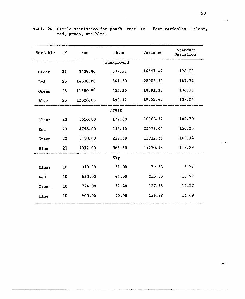
Table 24--Simp1e statistics for peach tree C: Four variables - clear,red, green, and blue.

Variable N Sum Hean Variance StandardDeviation

Background

Clear 25 8438.00 337.52 16407.42 128.09

Red 25 14030.00 561. 20 28003.33 167.34

Green 25 11380·00 455.20 18591. 33 136.35

Blue 25 12328.00 493.12 19055.69 138 •04-----------------------------------------------------------------------

Fruit

Clear 20 3556.00 177.80 10963.32 104.70

Red 20 4798.00 239.90 22577 .04 150.25

Green 20 5150.00 257.50 11912.36 109.14

Blue 20 7312.00 365.60 14230.98 119.29-----------------------------------------------------------------------

Sky

Clear 10 310.00 31.00 39.33 6.27

Red 10 650.00 65.00 255.33 15.97

Green 10 774.00 77 .40 127.15 11. 27

Blue 10 900.00 90.00 136.88 11.69

Table 25--Variance and covariance matrices for peach tree C Fourvariables - clear, red, green, and blue.

51

Variable Clear Red Green Blue

Background

Clear 16407.42 21324.43 17416.76 17615.56

Red 21324.43 28003.33 22675.83 22904.26

Green 17416.76 22675.83 18591. 33 18592.60

Blue 17615.56 22904.26 18592.60 19055.69-----------------------------------------------------------------------Fruit

Clear 10963.32 15542.08 11391. 26 12367.07

Red 15542.08 22577.04 16225.63 17382.69

Green 11391.26 16225.63 11912.36 12843.15

Blue 12367.07 17382.69 12843.15 14230.98-----------------------------------------------------------------------Sky

Clear 39.33 91.33 66.44 65.77

Red 91. 33 255.33 170.00 158.66

Green 66.44 170.00 127.15 127.55

Blue 65.77 158.66 127.55 136 •88

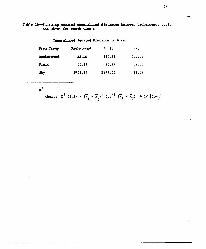
52

Table 26--Pairwise squared generalized distances between background, fruitand skyl! for peach tree C •

Generalized Squared Distance to Group

From Group

Background

Fruit

Sky

1.!

Background

23.1053.22

3951.24

Fruit

120.11

25.24

2272.05

Sky

630.08

82.33

11. 02

53

Table 27--Simp1e statistics for peach tree C: Three variables - clear,red, and blue.

Variable N Sum Mean Variance StandardDeviation

Background

Clear 25 8438.00 337.52 16407.42 128.09

Red 25 14030.00 561. 20 28003.33 167.34

Blue 25 12328.00 493.12 19055.69 138.04-----------------------------------------------------------------------Fruit

Clear 20 3556.00 177 .80 10963.32 104.70

Red 20 4798.00 239.90 22577.04 150.25

Blue 20 7312.00 365.60 14230.98 119.29-----------------------------------------------------------------------Sky

Clear 10 310.00 31.00 39.33 6.27

Red 10 650.00 65.00 255.33 15.97

Blue 10 900.00 90.00 136.88 11.69

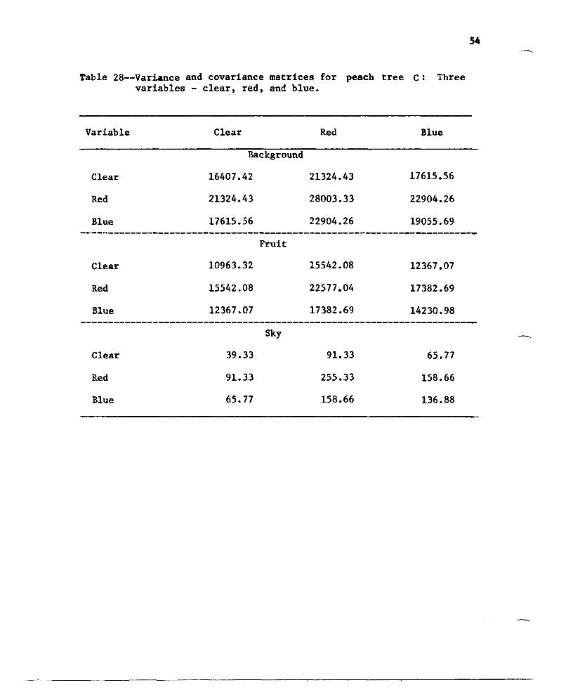
Table 28--Variance and covariance matrices for peach tree c: Threevariables - clear, red, and blue.

54

Variable

Clear

Red

Blue

Clear

Red

Blue

Clear

Red

Blue

Clear

Background16407.42

21324.43

17615.56

Fruit10963.32

15542.08

12367.07

Sky

39.33

91. 33

65.77

Red

21324.43

28003.33

22904.26

15542.08

22577 .04

17382.69

91. 33

255.33

158.66

Blue

17615.56

22904.26

19055.69

12367.07

17382.69

14230.98

65.77

158.66

136. 88

55

Table 29--Pairwise squared generalized distances between background. fruitand sky!/ for peach tree C •

Generalized Squared Distance to Group

From Group

Background

Fruit

Sky

!/

Background

20.33

42.90

3718.57

Fruit

82.71

21. 07

1302.59

Sky

94.32

67.58

10.70

56

Table 30--Simp1e statistics for peach tree c: Three variables - red,green, and blue.

Variable N Sum Hean Variance StandardDeviation

Background

Red 25 14030.00 561. 20 28003.33 167.34

Green 25 11380.00 455.20 18591. 33 136.35

Blue 25 12328.00 493.12 19055.69 138.04-----------------------------------------------------------------------

Fruit

Red 20 4798.00 239.90 22577 .04 150.25

Green 20 5150.00 257.50 11912.36 109.14

Blue 20 7312.00 365.60 14230.98 119.29-----------------------------------------------------------------------Sky

Red 10 650.00 65.00 255.33 15.97

Green 10 774 •00 77 •40 127.15 11.27

Blue 10 900.00 90.00 136.88 11.69

Table 31--Variance and covariance matrices for peach tree C: Threevariables - red, green, and blue.

57

Variable

Red

Green

Blue

Red

Green

Blue

Red

Green

Blue

Red

Background28003.33

22675.83

22904.26

Fruit22577.04

16225.63

17382.69

Sky255.33

170.00

158.66

Green

22675.83

18591.33

18592.60

16225.63

11912.36

12843.15

170.00

127.15

127.55

Blue

22904.26

18592.60

19055.69

17382.69

12843.15

14230.98

158.66

127.55

136.88

Table 34---Variance and covariance matrices for peachtree Cvariables - clear, green, and blue.

Three

60

Variable Clear

Background

Green Blue

Clear

Green

Blue

Clear

Green

Blue

Clear

Green

Blue

16407.42

17416.76

17615.56

10963.32

11391.26

12367.07

39.33

66.44

65.77

Fruit

Sky

17416.76

18591. 33

18592.60

11391. 26

11912.36

12843.15

66.44

127.15

127.55

17615.56

18592.60

19055.69

12367.07

12843.15

14230.98

65.77

127.55

136.88

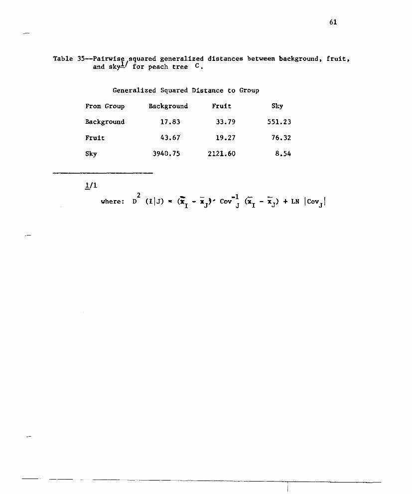
61

Table 35--Pairwise/squared generalized distances between background, fruit,and sky! for peach tree C.

Generalized Squared Distance to Group

From Group

Background

Fruit

Sky

1/1

Background

17.83

43.67

3940.75

Fruit

33.79

19.27

2121. 60

Sky

551.23

76.32

8.54

where:

62

Table 36--Simp1e statistics for peach tree C: Three variables - clear,red, and green.

Variable N Sum ~1ean Variance StandardDeviation

Background

Clear 25 8438.00 337.52 16407.42 128.09

Red 25 14030.00 561.20 18003.33 167.34

Green 25 11380.00 455.20 18591.33 136 •35-----------------------------------------------------------------------

Fruit

Clear 20 3556.00 177.80 10963.32 104.70

Red 20 4798.00 239.90 22577 .04 150.25

Green 20 5150.00 257.50 11912.36 109.14-----------------------------------------------------------------------Sky

Clear 10 310.00 31.00 39.33 6.27

Red 10 650.00 65.00 255.33 15.97

Green 10 774 •00 77 •40 127.15 11.27

Table 37--Variance and covariance matrices for peach tree C: Threevariables - clear, red, and green.

63

Variable

Clear

Red

Green

Clear

Red

Green

Clear

Red

Green

Clear

Background

16407.42

21324.43

17416.76

Fruit10963.32

15542.08

11391. 26

Sky39.33

91.33

66.44

Red

21324.43

28003.33

22675.83

15542.08

22577 .04

16225.63

91.33

255.33

170.00

Green

17416.76

22675.83

18591. 33

11391. 26

16225.63

11912.36

66.44

170.00

127.15

64

Table 38--pairwise/squared generalized distances between background, fruit,and sky.!. for peach tree C •

Generalized Squared Distance to Group

From Group

Background

Fruit

Sky

1/

Background

19.95

43.78

3885.89

Fruit

67.96

19.78

1200.67

Sky

74.42

39.64

9.65

65

Table 39--Simp1e statistics for peach tree D: Four variables - clear,red, green, and blue.

Variable N Sum Mean Variance StandardDeviation

Background

Clear 22 10836.00 492.54 37287.30 193.09

Red 22 14600.00 663.63 76052.43 275.77

Green 22 11966.00 543.90 47011.22 216.82

Blue 22 14878.00 676.27 40298.39 200.74-----------------------------------------------------------------------Fruit

Clear 17 6208.00 365.17 31003.02 176.07

Red 17 5818.00 342.23 72116.94 268.54

Green 17 7688.00 452.23 36840.94 191. 93

Blue 17 8648.00 508.70 34673.47 186.20-.---------------------------------------------------------------------Sky

Clear 22 2858.00 129.90 19.61 4.42

Red 22 8940.00 406.36 132.43 11.50

Green 22 5690.00 258.63 30.24 5.49

Blue 22 3406.00 154.81 25.77 5.07

Table 40--Variance and covariance matrices for peach tree D Fourvariables - clear, red, green, and blue.

66

Variable Clear Red Green Blue

BackgroundClear 31287.30 51023.25 41721.19 38137.74

Red 51023.25 76052.43 57155.01 51657.81

Green 41721.19 57155.01 47011.22 42089.93

Blue 38137.74 51657.81 42089.93 40298.39-----------------------------------------------------------------------Fruit

Clear 31003.02 45007.45 33351.45 31819.86

Red 45007.45 72116.94 46615.94 47594.07

Green 33351. 45 46615.94 36840.94 32994.57

Blue 31819.86 47594.07 32994.57 34673.47-----------------------------------------------------------------------Sky

Clear 19.61 38.12 17 •96 20.26

Red 38.12 132.43 37.66 46.35

Green 17 •96 37.66 30.24 18.88

Blue 20.26 46.35 18.88 25.77

61

Table 41--Pairwise squared generalized distances between background. fruit.and sky!1 for peach tree D.

Generalized Squared Distance to Group

From Group

Background

Fruit

Sky

!I

Background

30.49

34.32

20208.35

Fruit

50.53

30.58

14974.17

Sky

111.56

169.30

11. 04

68

Table 42---Simp1e statistics for peach tree D: Three variables - clear,red, and blue.

Variable N Sum Mean Variance StandardDeviation

Background

Clear 22 10836.00 492.54 37287.30 193.09

Red 22 14600.00 663.63 76052.43 275.77

Blue 22 14878.00 676.27 40298.39 200.74-----------------------------------------------------------------------Fruit

Clear 17 6208.00 365.17 31003.02 176.07

Red 17 5818.00 342.23 72116.94 268.54

Blue 17 8648.00 508.70 34673.47 186.20-----------------------------------------------------------------------Sky

Clear 22 2858.00 129.90 19.61 4.42

Red 22 8940.00 406.36 132.43 11.50

Blue 22 3406.00 154.81 25.77 5.07

Table 43--Variance and covariance matrices for peach tree D: Threevariables - clear, red, and blue.

69

Variables Clear Red

Background

Blue

Clear

Red

Blue

Clear

Red

Blue

Clear

Red

Blue

37287.30

51023.25

38137.74

31003.02

45007.45

31819.86

19.61

38.12

20.26

51023.2576052.43

51657.81

Fruit

45007.45

72116.94

47594.07

Sky

38.12

132.43

46.35

38137.74

51657.81

40298.39

31819.86

47594.07

34673.47

20.26

46.35

25.77

70

Table 44--pairwisi/squared generalized distances between background, fruit,and sky- for peach tree D.

Generalized Squared Distance to Group

From Group

BackgroundFruit

Sky

..1/

Background

26.39

29.93

20158.34

Fruit

32.28

26.61

14970.92

Sky

52.69

74.99

8.42

where:

71

Table 45--Simp1e statistics for peach tree D: Three variables - clear,red, and green.

Variable N Sum Mean Variance StandardDeviation

Background

Clear 22 10836.00 492.54 37287.30 193.09

Red 22 14600.-0 663.63 76052.43 275.77

Green 22 11966.00 543.90 47011. 22 216.82-----------------------------------------------------------------------Fruit

Clear 17 6208.00 365.17 31003.02 176.07

Red 17 5818.00 342.23 72116.94 268.54

Green 17 7688.00 452.23 36840.94 191. 93-----------------------------------------------------------------------Sky

Clear 22 2858.00 129.90 19.61 4.42

Red 22 8940.00 406.36 132.43 11.50

Green 22 5690.00 258.63 30.24 5.49

Table 46--Variance and covariance matrices for peach tree Dvariables - clear, red, and green.

Three

72

Variables Clear Red Green

Background

Clear 37287.30 51023.25 41721.19

Red 51023.25 76052.43 57155.01

Green 41721.19 57155.01 47011. 22.---------------------------------------------------------------------Fruit

Clear

Red

Green

31003.02

45007.45

33351. 45

45007.45

72116.94

46615.94

33351.45

46615.94

36840.94-----------------------------------------------------------------------Sky

Clear

Red

Green

19.61

38.12

17.96

38.12

132.4337.66

17.96

37.66

30.24

73

Table 47--pairwisi/squared generalized distances between background, fruit,and sky- for peach tree D.

Generalized Squared Distance to GroupFrom Group

Background

Fruit

Sky

1/

Background

25.05

28.78

10205.19

Fruit

37.31

25.34

7499.31

Sky

80.17

109.10

9.65

74

Table 48--Simp1e statistics for peach tree n: Three variables - clear,green, and blue.

Variable N Sum Mean Variance StandardDeviationBackground

Clear 22 10836.00 492.54 37287.30 193.09Green 22 11966.00 543.90 47011.22 216.82Blue 222 14878.00 676.27 40298.39 200.74-----------------------------------------------------------------------

FruitClear 17 6208.00 365.17 31003.02 176.07Green 17 7688.00 452.23 36840.94 191. 93Blue 17 8648.00 508.70 34673.47 186.20-----------------------------------------------------------------------

SkyClear 22 2858.00 129.90 19.61 4.42Green 22 5690.00 258.63 30.24 5.49Blue 22 3406.00 154.81 25.77 ~.07

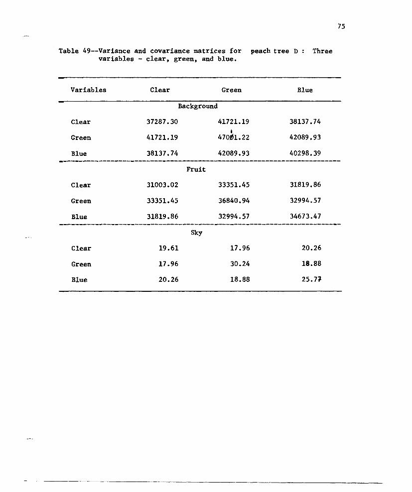
Table 49--Variance and covariance matrices for peach tree Dvariables - clear, green, and blue.

Three

75

Variables Clear

Background

Green Blue

Clear

Green

Blue

37287.30

41721.19

38137.74

41721.19I

470fl1.22

42089.93

38137.74

42089.93

40298.39-----------------------------------------------------------------------Fruit

Clear

Green

Blue

Clear

Green

Blue

31003.02

33351.45

31819.86

19.61

17.96

20.26

Sky

33351. 45

36840.94

32994.57

17.96

30.24

18.88

31819.86

32994.57

34673.47

20.26

18.88

25.71-

76

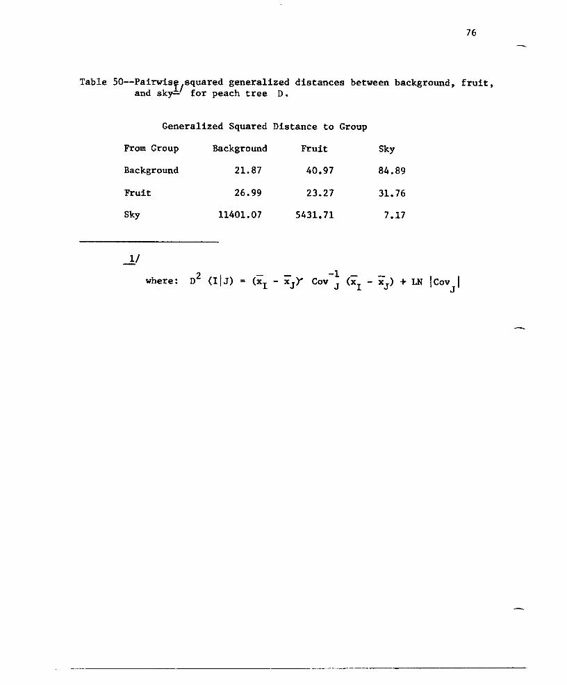
Table 50--PairwiSt/squared generalized distances between background, fruit,and sky- for peach tree D.

Generalized Squared Distance to GroupFrom Group

Background

Fruit

Sky

-1./

Background

21. 87

26.99

11401. 07

Fruit

40.97

23.27

5431.71

Sky

84.89

31. 76

7.17

where:

77

Table 51--Simp1e statistics for peach tree D: Three variables - red,green, and blue.

Variable N Sum Hean Variance StandardDeviationBackground

Red 22 ',14600.00 663.63 76052.43 275.7700

Green 22 .11966.00 543.90 47011. 22 216.82

Blue 22 .14878.00 676.27 40298.39 200.74------------------------------------------------------------------------Fruit

Red 17 5818.00 342.23 72116.94 268.54

Green 17 7688.00 452.23 36840.94 191.93

Blue 17 8648.00 508.70 34673.47 186.20-----------------------------------------------------------------------Sky

Red 22 8940.00 406.36 132.43 11.50

Green 22 5690.00 258.63 30.24 5.49

Blue 22 3406.00 154.81 25.77 5.07

Table 52--Variance and covariance matrices for peach tree Dvariables - red, green, and blue.

Three

78

Variables Red

Background

Green Blue

Red

Green

Blue

Red

Green

Blue

Red

Green

Blue

76052.43

57155.01

51657.81

72116.94

46615.94

47594.07

132.43

37.66

46.35

Fruit

Sky

57155.01

47011.22

42089.93

46615.94

36840.94

32994.57

37.66

30.24

18.88

51657.81

42089.93

40298.39

47594.07

32994.57

34673.47

46.35

18.88

25.77

79

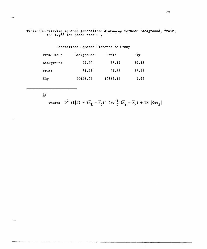
Table 53--Pairwise squared generalized distances between background, fruit,and skyl! for peach tree D •

Generalized Squared Distance to Group

From Group

Background

FruitSky

1/

Background

27.40

31.28

20126.45

Fruit

36.19

27.83

14882.12

Sky

59.18

76.23

9.92