PREHATCH AND POSTHATCH GROWTH OF FISHES­A GENERAL MODEL

JAMES R. ZWEIFEL AND REUBEN LASKER1

ABSTRACT

The developmental stages of fish eggs and the growth of larval fishes of several species can berepresented by a Gompertz-type curve based on the observation that in widely different living systems,exponential growth tends to undergo exponential decay with time. Further, experimental studies andfield observations have shown that the effect of temperature on the growth process follows the samepattern, i.e., the rate of growth declines exponentially with increasing temperature. Evidence suggeststhat prehatch growth rates determine ideal or optimum trajectories which are maintained after hatchin the middle temperature range but not at either extreme. Also, posthatch growth exhibits atemperature optimum which is not apparent in the incubation period. These studies have also shownthat for the same spawn both the prehatch and yolk-sac growth curves reach asymptotic limitsindependent of temperature. Other biological events (e.g., jaw development) occur at the same size forall temperatures.

The growth of post-yolk-sac larvae follows a curve of the same type and hence the posthatch growthtrajectory may be represented by a two-stage curve. For starving larvae, the second stage shows adecline in size but maintains the same form, i.e., the rate of exponential decline decreases exponentiallywith time.

Recent success in spawning and rearing marinefish larvae at the Southwest Fisheries Center(SWFC) (Lasker et al. 1970; May 1971; Leong 1971)has made possible a much more fundamentalexamination of the growth process than has here­tofore been possible. Controlled laboratory exper­iments can now be utilized to investigate both theinherent nature of the growth-process as well asthe effect of some environmental factors.

Considerable care is required, however, in con­structing a model2 which is meaningful bothmathematically and biologically. For example,almost all growth models currently in use can bederived as variations of the differential equation:

dW = 1/W m_KW" (1)dt

dL, ,

ordt

= 1/'Lm

- K'L" (la)

(von Bertalanffy 1938; Beverton and Holt 1957;Richards 1959; Chapman 1961; Taylor 1962) where

lSouthwest Fisheries Center La Jolla Laboratory, NationalMarine Fisheries Service, NOAA, La Jolla, CA 92038.

2A model is here conceived to be a mathematical representa­tion of change in length or weight with time under measureableenvironmental conditions.

Manuscript accepted March 1976.~'ISHERY BULLETIN: VOL. 74, NO.3, 1976.

W is weight, L is length, and 1/, K, m, n, m; and n'arearbitrary constants. These are the equations usedmost often to describe growth as a function ofanabolic and catabolic processes of metabolism.The rate of anabolism, 'I), is considered to beproportional to Will and the rate of catabolism, K,

proportional to W". Equation (Ia) requires, inaddition, the allometric relationship W = qLP

,

where again q and p are arbitrary constants. Inpractice a dilemma arises from the fact that whilesuch models yield a good empirical fit to the data,the estimates of parameters 1/ and K are oftennegative, thereby negating the assumptions onwhich the model is based. For n = 1 and m = 0, 1,2, respectively, Equation (I) gives rise to the vonBertalanffy growth in length, Gompertz, andlogistic growth functions. Although we have not asyet made any extensive comparisons, the fact thatfor m>1 and n = 1, 1/ and K must be negative,suggests that in many instances the Gompertz andlogistic rather than the von Bertalanffy functionsmay provide more appropriate models of fishgrowth. In particular, the simple von Bertalanffygrowth model has no inflection point and hencecurves such as the generalized von Bertalanffy,Gompertz, or logistic must be used when an in­flection in the growth trajectory is evident.

Laird et al. (1965) have presented a Gompertz­type mathematical model of growth based on the

609

FISHERY BULLETIN: VOL. 74, NO.3

dW(t) = yet) Wet)dt

where Wo is weight at t = 0, A o is the specificgrowth rate at t = 0, a is the rate of exponentialdecay and the specific growth rate at time t, A, =

A -111oe •Laird et al. (1965) indicated that an additional

growth component not included in the Gompertzequation may be due to the accumulation ofproducts that are not self-reproducing or torenewal systems that are not in exact phys­iological equilibrium and suggested the com­pound growth curve:

observation that the specific growth rate dW/ Wdtof animals and their parts tends to decay expo­nentially with increasing age. They have shownthat this relation offers a practical means ofanalyzing the growth of parts of embryonic andpostnatal animals (Laird 1965a), the growth oftumors (Laird 1964, 1965b), whole embryos of anumber of avian and mammalian species (Laird1966a), and early stages of postnatal growth of avariety of mammalian and avian organisms (Laird1966b). Further, Laird (1966b, 1967) has shownthat postnatal growth of a variety of mammalianand avian organisms can be fitted by compoundingthis model with a linear growth process beginningat birth and extending on beyond the asymptoticlimit of the underlying Gompertz growth process.Overall growth is assumed to be genetically de­termined by programming only the initial specificgrowth rate and the rate of exponential decay,these governing growth processes then act on agenetically determined original mass to producethe observed course of growth to a final limitingsize characteristic of the species and individual.

Mathematically, these assumptions are de­scribed by the two equations:

(3)Jt W

W = WG + f3 ~ dto M

where WG is the mass due to the Gompertz growthprocess, f3 is the rate of linear growth, and M is theasymptotic limit of the growth process. She alsosuggests that this linear process starts in the earlyembryonic period, if not at conception. For the ageinterval covered in this paper, however, the lineargrowth component (W - WG ) was not found to beimportant.

Several characteristics of the curve are worthyof mention:

1. The asymptotic limit M is Wo Exp (Ao/a).2. The point of inflection (tl , ~) =

[~ln(Ao/a), WoExP(~O -l)J.3. The zero point on the time scale may

be shifted to any point t", without changing theform of the equation with new parameters W'" =W (L\), A", = Aoe--<r'" where a remains un­altered.

The fundamental concept of the Laird­Gompertz model is one of change in weight ormass with time, being due primarily to the self­multiplication of cells and genetically determinedlimitations on the growth parameters. The use oflength as the measured variable is thus a matter ofconvenience due to the fact that weight measure­ments are much more time consuming, especiallyin early larval growth, but also in juvenile andadult fishes. As indicated in Equation (la), if a trueallometric relationship existed, the choice would beunimportant. However, all experimental evidenceindicates that both length and weight can bedescribed by a Gompertz-type curve. Hence, it canbe shown that 1) the growth rate for both changescontinually with time and 2) the form of thelength-weight relationship will change continuallyexcept for two special instances. Laird et al. (1968)has shown that this occurs only when the rates ofexponential decay are the same and either the twomeasured variables begin growth at differenttimes at the same initial rate or at different ratesat the same time. In all other cases the allometricplot will be nonlinear. For

(2)

- ay(t)dy(t)

dt

which have the solution

"In the usual Gompertz representation the rate of exponentialgrowth is assumed to decline logarithmically as W approaches

.6. dWthe asymptote M = Woe • , I.e., (JI = 11 WIn(M/ W). and

610

ZWEIFEL and LASKER: PREHATCH AND POSTHATCH GROWTH OF FISHES

the length-weight relationship is

!nW ~ !nW, + K+~A;'-!~~/L,~ "" 1(4)

Only when a = f3 does the relationship reduce tothe linear form

InW = In Wo + IJ(: In (LI Lo)·

then W(t) = Me- Ke -at

,

or In[-ln(W(t)/M)] = In K-'at,

and hence the logarithm of the logarithm of theratio of size to the asymptotic limit M with thesign changed will be linearly related to time t withparameters In K and -a. Wo may be obtainedfrom the relationship In M = In Wo + K. Note: Fordecreasing curves, use the reciprocal of the ob­served values.

INITIAL ESTIMATES

Equation (2) may be rewritten as follows:

6':,.01---C0~0::-2 --'-:0":-.04~006~'f:0.1---C--:0:':2--L-;0~.4 -'-:0:':6"='0'='"e~,--:-----'--:4--'-:6~e ~IO

WEIGHT (mQ)

VARIABILITY, ESTIMATION, ANDTRANSFORMATION BIAS

It is an unfortunate circumstance that thedetermination of the "best" estimation procedurecan rarely be separated from the determination ofthe "best" mathematical model, i.e., there is norecognized best estimation procedure except insome specialized instances. This is brought aboutby the fact that almost all parametric estimationprocedures assume some information concerningthe form and stability of the "error" distribution.This requires, at the very least, the knowledge thatthe variance is constant and, at the most, the exactform of the error distribution. Since the term"error" in the biological sciences takes a meaningquite different from that in the physical andmathematical sciences in that it represents, in themain, natural variability rather than measure­ment or experimental error and since naturalvariability is large (especially so in cold-bloodedorganisms), few a priori assumptions can be made.

Since most estimation procedures assume anormal distribution of errors at each point alongthe curve with equal variance (homoscedasticity),the obvious approach, when no more plausiblealternative is available, is to fit the situation tothis mold.

Some general recommendations are helpful."Although no clear rule may be safely offered forthe taking of logarithms to reduce data to man­ageable configurations, nevertheless, this trans­formation (logs) is probably the most common ofall. Almost all data that arise from growth phe­nomenon, where the change in a datum is likely tobe proportional to its size and hence errors aresimilarly afflicted, are improved by transforms totheir logarithms" (Acton 1959: 223). Specifically, itcan be shown that the logarithmic transformationwill induce homoscedasticity in those instances

K = Ao/aLet

and

FIGURE l.-Length-weight relationship in larval anchovies: Solidline fitted from log W = a + b log L; dashed line fitted fromEquation (4); estimates are coincident up to 10 mm.

As shown in Figure 1, departure from linearitywill not always be great, but for extrapolation theeffect of overestimation at larger sizes maybecome serious.

Throughout this paper, growth will, by necessi­ty, be measured in terms of length rather thanweight even though the model equation isdeveloped from the opposite point of view. Itshould be remembered, however, that no allomet­ric relationship is assumed, i.e.,no relationshipsamong the two sets of parameters are assumedexcept as they are jointly a function of age.

100eo

60

40

] 20 0.

:I:f-

~10

W e..J

611

FISHERY BULLETIN: VOL. 74, NO.3

4 Paloma, P. Unpublished data available at SWFC.

Not unexpectedly, variation in weight exceedsthat of length and both decrease with increasingage.

The question of normality and its relationship tohomoscedasticity is more tenuous, but again somehelp is available. In practical work, it is generallyassumed that both :r and log :r can be regarded asnormally distributed as long as the coefficient ofvariation C = olJ.1< Ih or a,o" J' <0.14 (Hald 1952:164). This allows transformation for one desidera­tum without noticeably affecting another.

Paloma (see footnote 4) collected one or twosamples per month of laboratory-reared anchoviesfor a period of nearly 2 yr. Approximately 25 fishwere taken for each sample. We examined nor­mality in terms of skewness (G1) and kurtosis(mean absolute deviation A). Although sample

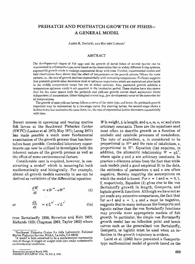
where the standard deviation is proportional tothe population mean, i.e., 0 = f3J-l or log 0 = log f3 +log J-l. Hence, a plot of log 0 on log J-l will have a slopeof unity and the antilog of the intercept will definethe proportionality constant. Plots of log a on log /lwere made for several experiments where datawere available for extended periods of time. Noneof the regression coefficients was significantlydifferent from unity. These experiments cover avariety of life stages and environmental situa­tions from controlled laboratory experiments onlarval anchovies (Lasker et a!. 1970) to large tankfeeding of anchovies captured from the wild at 75mm (Paloma, SWFC, unpub!. data) to samples ofadult sardines obtained from bait boats (Lasker1970). Growth for the 75-mm anchovies was slowand much more uniform than for the other exper­iments as indicated by the mean square errors inTable 1. The analysis of covariance (Table 1) showsno difference in slope for either length or weightfrom larval, juvenile, and adult fishes. The average

. slopes are 0.9981 for larvae and adults and 1.1061for juveniles. With a slope of unity, the propor­tionality constant can be estimated by Exp (I no ­In/l). The results from the several experiments areshown below:

ol/lLength Weight L log L W log W

G1(/lGl = 0) > 19 17 24 16:s 14 16 19 17

A(J-lA = 0.7979) > 18 17 17 17:s 15 16 16 16

sizes are small, in terms of positive (>mean) andnegative « mean) coefficients, the transformationwas effective in normalizing both fish weight andlength as shown below:

Analysis of covariancedeviations from

log u = a + f3 log p. reg resslon

For these same samples, length and weight wereassumed bivariate-log normal and confidenceregions were calculated for each sample. On theaverage, 96% of the observations fell within the95% confidence ellipse.

In summary, there is strong evidence that thelogarithmic transformation will be required tostabilize the variability in all phases of fish growthand that such a transformation will support theassumption of a normal distribution at least in theintermediate size range (75-100 mm) and mostlikely at other sizes as weI!.

Seemingly then, the conditions have been metfor implementation of either the maximumlikelihood or least squares estimation process.However, two problems remain, neither of whichhas an entirely satisfactory solution. The first, theabsence of an explicit solution of the normalequations, arises because the parameters enter themodel in a nonlinear manner and, as is usual in

TABLE 1.-The relationship of mean and standard deviation forboth length and weight measurements in fishes.

a p dl •... m.s.

Larvae and adults:Length' expo 1 -1.5568 1.6979 6 0.3308 0.0551

exp.2 -0.8003 0.8281 8 0.7167 0.0896Weight' expo 1 -0.4192 1.0373 6 0.1572 0.0262

exp.2 -0.4852 1.0077 8 0.4241 0.0530Length2 -1.6093 1.0848 60 2.2933 0.0382Weight' -0.4748 0.7906 60 2.5913 0.0432

Within 148 6.5134 0.0440Between 5 0.1425 0.0285Common 153 6.6559

F = 0.0285/0.0440 = 0.65

'Lasker et al. (1970), larval anchovies.'Lasker (1970), adult sardines.'Paloma: unpublished data available at SWFC, Juvenile an­

chovies .

F = 0.0002/0.p083 = 0.02

Juveniles:Length' -1.3975 1.1644 31 0.3658 0.0118Weight' -0.8000 1.1029 31 0.1511 0.0048

Within 62 0.5169 0.0083Between 1 0.0002 0.0002Common 63 0.5171

0.390.330.200.13

0.120.120.060.04

Lasker et al. (1970):Experiment 1Experiment 2

Paloma4

Lasker (1970)

612

ZWEIFEL and LASKER: PREHATCH AND POSTHATCH GROWTH OF FISHES

RESULTS

Growth Cycles

FIGURE 2.-Change in length of yolk-sac and feeding larvalanchovies at two temperatures, 17° and 22°C from Kramer andZweifel (1970); curves are two-cycle Laird-Gompertz.

I mean ± 2 SO

22"C20

Previous work on the growth of larval anchovies(Kramer and Zweifel 1970) suggested that theLaird form of the Gompertz equation mightprovide a useful model of larval growth. Figure 2reveals several phenomena found to be almostuniversal in larval growth: 1) there is a moderateincrease in length during the interval followinghatch that is followed by 2) a period of minimalgrowth accompanied by nearly uniform variabili­ty, and 3) at the onset of feeding, the mean sizeincreases rapidly with variability proportional tothe square of the mean size.

Farris (1959) noted the rapid leveling off ingrowth following hatch for the Pacific sardine andthree other species and approximated the growthrate by two discontinuous curves and indicatedthat "a more detailed study would probably reveala nonlogarithmic continuous growth function."

EE 0

:t: 24~~:0::

20 17"Cw-l

16

12

8

4

at ! ! ! ! ! ! ! 1 ! ! ! ! ! !

0 4 8 12 16 20 24 28 32 36

DAYS AFTER HATCHING

situations of this kind, an iterative procedure isrequired. The one employed for this paper isMarquardt's algorithm (Conway et al. 1970).Procedures such as this are usually justified on thebasis that for large samples and independentobservations the estimates obtained are "veryclose" to those which would be obtained by plot­ting the likelihood function itself (Box and Jen­kins 1970: 213). In truth, the small sample bias andvariability of such estimates remains unknown. Ingrowth data the second problem is that sequentialobservations are not likely to arise from entirelyindependent processes. This fact is usually man­ifested as a series of runs above and below a fittedcurve rather than random variation. One simpleexplanation is that growth is in reality a series ofasymptotic curves and that oscillations around afitted curve indicate more than one growth cycle.In this case, the basic assumption of the estima­tion procedure and the likelihood function itselfwill not be met. No satisfactory solution to thisproblem has been proposed and none is profferedhere. However, since the same larvae were notmeasured at different ages and since correlatedobservations usually have little effect on theestimates of mean values, such estimates willlikely not be seriously biased. Using these es­timates, "goodness of fit" is examined through themagnitude of the residual mean square and thepattern of residuals along the growth curve, ratherthan using significance tests or confidenceintervals.

One further point often considered but leftunsaid is the effect of transformations on theestimated means. Such changes of scale can lead toserious biases and errors in interpretation,especially when the coefficient of variation islarge. When the exact form of the error distribu­tion is known the bias can usually be determinedmathematically. For the log normal, for example,it is necessary to add one-half of the error meansquare before calculating the antilog mean. Un­fo,rtunately, in practical work, it is generallyimpossible without very large samples, to deter­mine the distributional form. As stated above, formany situations, x and log x can both be consideredto be normally distributed. In these intermediatecases, however, the bias correction for log x will besmall so, that as a general rule; one can state thatwhenever a transformation is made, the correctionfor transformation bias should be used.

613

FISHERY BULLETIN: VOL. 74, NO.3

a -a em(l - .-/lTopt)opt - 0

was used to fit the growth data from all exper­iments and provided an excellent fit except at thehighest temperature where growth was alwaysoverestimated. This suggested a temperatureoptimum with growth rates decreasing as theabsolute difference IT - Toptl increases. FollowingStinner et aJ. (1974), who used a different temper­ature function, we assumed symmetry around theoptimum.

Using Equation (5a), the origin of the tempera­ture scale may easily be shifted to the optimumTopt by the relationships:

(5)

(5a)

and

where

0

5.5 0

0

.....E ••E • • •:I: •~C)zW...J

t:>

0 JACK MACKERELt:> SENORITA• SQUARETAIL0 SARDINE

15\'0 2 4 6 8 10 12

DAYS AFTER HATCHING

FIGURE 3.-Change in length of yolk-sac and starving larvae;curves are two-cycle Laird-Gompertz.

Growth From Hatch to Depletionof Yolk Sac

The characteristics of the early posthatchgrowth of larval fishes is more completely de­scribed by Lasker (1964). In this series of exper­iments, growth in length of the Pacific sardine,Sardinops sagax, was measured for up to 10 daysfollowing hatching at 12 temperatures in therange 11°-21.3°C. The parameters of a singlestage Laird curve (Equation 2) were estimated foreach of these experiments. Data only up to the daypreceding the first decrease in size were used inthe calculations.

Even though for such short time series, theparameters are highly correlated due to near­redundancy of one of the parameters, two obser­vations were striking; there was a nearly constantestimated hatching length of about 3.75 mm anda nearly constant estimated maximum length ofabout 6.1 mm. Accordingly, those experimentswith hatching lengths near 3.75 mm and a mea­sured increase in size of at least 3 days were fittedto the reparameterized model:

L(t)r = LoeK(l-.-ar/)

where K = Ao I aT T

and the T subscript indicates temperature in °C. Aplot of aT on temperature revealed anotherLaird-Gompertz curve approaching an asymptoteat higher temperatures.

A five parameter model:

Although the single stage model used by 6.5Kramer and Zweifel (1970) provides an adequategrowth curve, two growth cycles are evident: oneextending from hatching to the depletion of theyolk sac and the other a more rapid growth at theonset of feeding. Thus, a two-stage model wasused to obtain the curves in Figure 2. The fittingprocedure is outlined in the Appendix.

It is evident that early larval growth of thisspecies can be represented by a two-stage Lairdgrowth curve. The charcteristics of the growthcurves of feeding larvae, i.e., the second cycle, maybe related to several environmental factors ofwhich the two most important are probably foodration and temperature. However, an examinationof data available on nonfeeding larvae (Figure 3)indicated that even in food-limited situations,change in size may be represented by the two­stage Laird curve.

614

ZWEIFEL and LASKER: PREHATCH AND POSTHATCH GROWTH OF FISHES

and letting ~ = IT- Toptl

we have the symmetric relationship

a = a emopt(l-e·PA) (5b)T opt .

Substituting Equation (5b) for Equation (5a) andtreating Top! as an unknown parameter, a sixparameter model was fitted to the growth datawith the results shown in Table 2.

TABLE 2.-Growth in length of yolk-sac larvae of the Pacificsardine at several temperatures.

Length Temper-Age ature

Observed' Estlmated2 SE (days) (·C) N

3.76 3.72 0.15 0.00 11.00 74.30 4.27 0.27 1.00 44.78 4.71 0.50 2.00 44.97 5.06 0.25 3.00 23.77 3.72 0.20 0.00 12.00 94.50 4.40 0.24 1.00 114.71 4.91 0.29 2.00 85.04 5.28 0,44 3.00 65.50 5.54 0.38 4.00 33.73 3.72 0.16 0.00 13.00 84.50 4.55 0.23 1.00 174.97 5.12 0.41 2.00 115.46 5.49 0.45 3.00 94.80 4.72 0.20 1.00 14.00 225.39 5.33 0.27 2.00 195.65 5.67 0.36 3.00 93.93 4.08 0.13 0.30 14.20 114.08 4.09 0.13 0.30 14.30 55.14 4.89 0.44 1.00 15.00 175.59 5.51 0.35 2.00 205.96 5.81 0.32 3.00 103.71 3.72 0.25 0.00 16.00 215.01 5.07 0.25 1.00 195.68 5.67 0.26 2.00 235.99 5.91 0.15 3.00 116.23 6.00 0.11 4.00 93.74 3.72 0.22 0.00 16.80 145.20 5.21 0.16 1.00 165.77 5.78 0.20 2.00 226.14 5.97 0.20 3.00 133.69 3.97 0.10 0.10 17.80 55.27 5.38 0.19 1.00 165.86 5.88 0.23 2.00 226.06 6.D1 0.22 3.00 193.71 3.72 0.21 0.00 18.80 45.46 5.53 0.18 1.00 185.98 5.95 0.21 2.00 256.09 6.04 0.15 3.00 183.73 3.72 0.10 0.00 19.60 45.36 5.58 0.19 1.00 185.73 5.97 0.17 2.00 155.93 6.04 0.25 3.00 165.10 4.83 0.12 0.50 20.50 125.46 5.45 0.18 1.00 125.43 5.32 0.03 1.00 21.30 35.90 6.00 0.13 3.00 S

'From Lasker (1964).2Calculated from Equations (5) and (Sb) with parameters L. =

3.716, K - 0.4872, a opt - 1.8523, m - 3.3878, f3 - 0.0490, andTopt = 19.38.

Growth From Fertilization to Hatch

Coincident to the investigation of early larval

growth, a study of the incubation times for thesardine showed that they also could be character­ized by a Laird-Gompertz curve. The fitting ofEquation (5a) with aT being incubation timeshowed no bias at any point along the curve(Figure 4). Unlike the posthatch growth curves,however, no evidence of a temperature optimumwas found, i.e., incubation time did not increase athigh temperatures. One possible explanation isthat larvae which expire cannot be included andhence mortality introduces a negative bias in theestimate of average or median incubation time.

The question arises whether changes in growthrates occur at hatching, i.e., is there a single curvefrom fertilization to onset of feeding? It can beshown that under the Laird-Gompertz modelwhere growth is approaching a common asymp­tote from a common origin, i.e. fertilization, theincubation time IT is simple multiple of the decayrate a T' From Equation (5) we may solve for thetime to hatch IT at size 4. to obtain:

~ K ~IT = In la .K-ln(L I1 / Lo ) T

Since incubation times were not available for alltemperatures used in the growth experiment, thesardine curve from Figure 4 was used to convertall data taken at temperatures less than optimumto time from fertilization and fitted to Equation(5).

The results for sardines indicated an increasingsize at hatch with increasing temperature whichwas not evidenced by the observed data and anoverestimate of size at temperatures less than14°C. It was thus concluded that a change ingrowth rate occurs at hatch, the more noticeably atextreme temperatures and that the prehatch curvemust be estimated separately.

The parameters of the prehatch growth curveswere obtained by fitting the equation

(6)

to only data obtained less' than 12 h followinghatch. The average estimated hatching size was3.73 mm and the asymptotic limit was 6.13 mm.The plot for several selected temperatures isshown in Figure 5. Laird (1965a) has shown thatthe length scale may be standardized and logicallysimplified by expressing size relative to theasymptotic limit. Biological events such as

615

FISHERY BULLETIN: VOL. 74, NO.3

28

24

BAIRDIELLA

(6537,-7.1015,0.0650)*o

150 200

TURBOT(1012,-5.2103,0.0444)*

o

o

50 100

SENORITA

(8293,-7.6534,0.0624)*

SANDDAB

(1159,-5.1563,0.0629)*

o

o

150

JACK MACKEREL

(6910,-6.1172,0.0599)

50 100

PACIFIC MACKERELo

(3646,-6.4705,0.0535T

o

o

o

o

o

100 150

o 0

50

SHEEPHEAD

(830.3,-7.8980,0.0250)*

28

24

20

16

~ 12u~

l1J 80:::> 22I-<l:0:l1J 18a..:El1JI- 14

10

6

24

20

16

12

80

HOURS

FIGURE 4.-0bserved (0) and estimated (curve) (parameters in parentheses are 10 , m, and {3 for the-m(l _ e-IJT)

equation iT = 10e and' indicates time from stage III eggs) incubation times for anchovy,Engraulis mordax [combined data from Lasker (1964) and Kramer (unpub!. data) available atSWFC); hake, Merluccius productus; sheephead, Pimelometopon pulchrum; bairdiella, Bairdiellaicistia; jack mackerel, Trachurus symmetricus; sardine, Sardinops sagax; Pacific mackerel,Scomber japonicus (Watanabe 1970); sanddab, Citharichthys stigmaeus; turbot, Pleuronichthysdecurrens; senorita, Oxyjulis californica.

developmental egg stages, hatching, and develop­ment of the functional jaw occur at fixed pointsalong the curves. Ahlstrom (1943) reported time toseveral developmental egg stages at different

temperatures from field observations. In addition,Lasker (1964) showed incubation times and time tothe development of the functional jaw for a widerrange of temperatures. Each of these events can

616

ZWEIFEL and LASKER: PREHATCH AND POSTHATCH GROWTH OF FISHES

Prehatch Growth Curves forOther Species

In addition to incubation times for the northernanchovy, Kramer" recorded time to severaldevelopmental egg stages. Also, Lasker (1964)provided time to hatch from stage IV6 (Table 5).Further, Hunter (pers. commun.) indicates that

Incubation Times

Incubation times were available for severalother species. The fitting of Equation (5a) for eachspecies showed no clear bias at any point along thecurve (Figure 4). As for the sardine, no evidence ofa temperature optimum appeared for any of thespecies in the temperature ranges used in theexperiments. However, it was observed that thedecay parameter was relatively constant varyingfrom 0.03 to 0.09 with a mean value of 0.05. WhenEquation (5a) was fitted with the temperaturedecay parameter, /3, the same for all species,incubation times were closely approximated byEquation (5a) with parameters as shown in Table4.

The incubation curves used here differ sig­nificantly from those calculated from the classicalArrhenius equation: log (incubation time) = a +b/absolute temperature. Using this method, near­ly all species showed a characteristic under­estimate at the temperature extremes and over­estimates in the middle range as shown for thenorthern anchovy, Engraulis mordax (Figure 6).

14

13" II" 6.135.97

15"

8 10 126

/----~~~;.'iI~~~~XI.----l3.73 E1----"-=""-""'------13.55 E

4

J:f­(!)2

STAGE -IX 2 0 w-J-----~'-""'''''--'......-'''''--___i.3 ..J

I -"S"-'TA"'G.=..E"":llI"-----l1.15

I-Jlljf/ S"'T""AG"'E~1II""_____l0.29

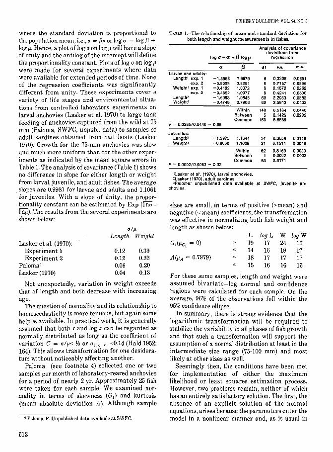
be identified as a fixed percentage point in Figure5 or the estimated value

tLT = In ( K )/CXT (7)K ~ In (LT / Lo)

as shown in Table 3.Lasker (1964) found that the functional jaw did

not develop at the lowest two temperatures inagreement with the result that the critical sizewould not be reached until well after yolkabsorption.

E Q8E

0.5J:f-

~ 0.4w..J

0.3

0.9

~ 0.7U)

0l-

EE

DAYS FROM FERTILIZATION

FIGURE 5.-Prehatch growth curves estimated from Equations (5)and (5a) for the Pacific sardine.

'Unpublished data available at SWFC."Stages of embryological development are those described by

Ahlstrom (1943).

TABLE 3.-0bserved (Obs.) and estimated (Est.)1 time in hours to developmental egg stages2 , hatch, and appearance of the functional jawof the Pacific sardine.

Ahlstrom (1943) Lasker (1964)

Stage III Stage VI Stages VIII-IX Stage XITemp.

Incubation time Functional JawTemp.

(Oe) Obs. Es!. Obs. Est. Obs. Est. Obs. Es!. (oG) Obs. Es!. Obs. Es!.

13.5 20.4 20.1 41.8 42.9 62.5 63.2 82.6 85.4 11 140 13514.0 18.9 18.6 39.1 39.7 58.3 58.5 77.2 79.0 12 115 11414.5 17.4 17.3 36.6 36.8 59.4 54.3 72.2 73.3 13 93 96 213 21615.0 16.2 16.1 34.3 34.2 50.7 50.4 67.5 68.1 14 78.5 82.4 179 18515.5 14.9 15.0 32.1 31.9 47.2 46.9 63.1 63.4 15 68.1 71.0 156 16016.0 13.8 14.0 30.0 29.7 44.0 43.7 59.0 59.1 16 60.2 61.6 136 13816.5 28.1 27.7 41.1 40.8 55.1 55.2 17 53.7 53.8 119 12117.0 26.3 26.0 51.5 51.6 18 48.4 47.3 105 106

19 43.2 41.8 94 9420 39.3 39.2 85 8421 34.0 33.2 77 75

ILo - 0.0341, K - 5.20, (10 - 0.0317, m = 6.19, and P = 0.0489.'Egg stages are defined In Ahlstrom (1943).

617

FISHERY BULLETIN: VOL. 74, NO.3

DAYS FROM FERTILIZATION

DISCUSSION

2.852.80

EE

J:2.00 l-

e>zw..J

1.12

HATCH

STAGE IX:

STAGE =

STAGE :lZI

.....-:;2;..-'.---:'9;....--:':;..7._'5.•__--130 11° 4.31

I----/_ FUNCTIONAL JAW 4.20

1Jl),,.. ~ST~A""GE'_'m"'________iO.l8

Comparison with the sardine curves indicate thatsimilar events (Le., stages of development) occurrelatively later for the anchovy. Observed andestimated event times are shown in Table 5.

Except for size at hatch, development data forthe prehatch stage was not available for any otherspecies. The curves may, if desired, be easilyconstructed from the parameters as shown inTable 6.

FIGURE 7.-Prehatch growth curves estimated from Equations (5)and (5a) for the northern anchovy.

Nothing seems more true than the statement ofThompson (1942:158), "Every growth-problembecomes at last a specific one, running its owncourse for its own reasons. Our curves of growthare all alike-but no two are ever the same. Growthkeeps calling our attention to its own complexity.... not least in those composite populations whoseown parts aid or hamper one another, in any formor aspect of the struggle for existence."

The truth of this statement has been realized inthe disappointing search for growth models de­rived from physiochemical processes. While it istrue that the mathematical form of some equa­tions arrived at from metabolic considerations arethe same as those derived in other ways, more

0.00360

m fJ

-7.9531 0.0527 EE

-6.8216 0.0527 it;

0.0527<i

-6.4896 .,.-6.2486 0.0527 E

E-6.2322 0.0527

J:-5.5218 0.0527 l-

e>-5.4258 0.0527 Z

w..J

-5.4194 0.0527

-4.7059 0.0527

-4.1772 0.0527

0.003500.00340

I + TEMPERATURE (OK)

1.2 0.00330

TABLE 4.-Parameters for estimating incubation time I atcentigrade temperature T from the relationship IT =Iaem(l •• ''', for several fishes where fJ is the same for all species.

Species '0Sellorita

OxyJulls esllfornleus '6,103Bairdiella

Bslrdlella /e/stla '3,170Pacific mackerel

Seomber Japon/cus 3,580Jack mackerel

Trsehurus symmetr/eus 1,854Pacific sardine

Ssrd/nops ssgsx 2,121Northern anchovy

Engrsulls mordsx 1,389Speckled sanddab

C/thsr/chthys stlgmssus '984.6California sheephead

P/ma/omstopon pulchrum '1,316Turbot

P/suron/ehthys decurrens '1,065Pacific hake

Mer/uce/us produetus 699.2

'Time from stage III eggs.

2.2

larval anchovy, on the average, hatch at about 2.9mm.

Prehatch growth curves were obtained byfitting Equation (6) to hatch sizes of 2.85 at allobserved temperatures as shown in Figure 7.

FIGURE 6.-A comparison of two methods of fitting the tempera­ture-incubation time relationship in the northern anchovy.

2.0

-;A...c.

W~ 1.8i=z0

!iCO

1.6:::>U~

(l)OBSERVED9 •

0 LAIRD - GOMPERTZ1.4 ARRHENIUS EQUATION

i> COINCIDENT POINTS

618

ZWEIFEL and LASKER: PREHATCH AND POSTHATCH GROWTH OF FISHES

TABLE 5.-0bserved (Obs.) and estimated (Est.)' time in hours to developmental egg stages2, hatch, and appearance of the functional jawof the northern anchovy.

Kramer (unpubl. data) Lasker (1964)

Temp.Stage III Stage VI Stage VIII Stage XI Incubation time

Temp.Stage IV to hatch

(OC) Ops. Est. Obs. Est. Obs. Est. Obs. Est. Obs. Est. (OC) Obs. Est.

11.1 113 118.8 11 81 8312.5 98 95.1 12 65 7113.8 20 15.2 42 41.8 58 59.4 78 77.1 80 78.2 13 58 6115.2 15 12.6 35 34.6 50 49.1 65 63.7 63 64.7 16.8 38 3716.6 10 10.6 26 29.0 39 41.2 51 53.4 55 54.2 17.8 34 3318.0 9 9.0 24 24.6 35 35.0 44 45.4 49 46.0 18.8 31 2919.4 8 7.7 21 21.1 33 30.0 39 39.0 40 39.5 19.6 28 2620.8 6 6.7 19 18.4 28 26.1 35 33.8 36 34.3 20.5 25 24

'Estimates obtained from Equation (7) with parameters as shown In Table 6.2Egg stages are defined by Ahlstrom (1943).

TABLE 6.-Mathematical parameters for prehatch growth curves of six fishes. See text fornotation.

AveragesIze at

Species Lo K a o m fJ hatching

rrachurus symmetr/cus 0.0005 9.0986 0.0226 5.8338 0.0588 1.95Sard/nops sagax 0.0341 5.1918 0.0317 6.1876 0.0490 3.74Engraul/s mordax 0.0250 5.1493 0.0412 5.5338 0.0546 2.86Clthar/chthys st/gmaaus 0.1814 5.0600 0.0270 6.2898 0.0319 1.97OxYJul/s ca/llom/cus 0.0425 4.7164 0.0572 7.2126 0.0260 1.89P/euronlchthys decurrens 0.1843 3.2915 0.0480 4.5184 0.0528 3.00

often than not no meaningful biological interpre­tation of the metabolic parameters can be made.The essence of the growth equation used here isgenetically programmed processes of exponentialgrowth and of exponential decay of the specificgrowth rate. The most probable source of expo­nential growth is, of course, self-multiplication ofcells, the causes of decay are many but not wellunderstood. Laird (1964, 1965a, b, 1966a, b, 1967)has shown that this kind of relationship offers apractical means of analyzing growth of all tumors,as well as embryonic and postnatal growth of anumber of avian and mammalian species. We haveshown that at least the early stages of the growthof fishes follows a similar pattern.

As with other organisms, several growth cyclesexist in fishes. The number of such cycles whichwill be recognized is determined by the time scaleof measurements. We have used three cycles: 1)from fertilization to hatching, 2) from hatch toonset of feeding, and 3) feeding larvae.

In addition, we have observed that the temper­ature specific growth follows a similar pattern, Le.,exponential increase with an exponential decay ofthe temperature specific growth rate. In someinstances a temperature optimum exists beyondwhich the specific growth rate begins to decline,although this may be related to food requirementsat onset of feeding. Further, we have observed

that for the same spawn 1) the asymptotic limit ofeach growth cycle is independent of temperatureand 2) the biological events such as developmentalegg stages, hatching, functional jaw development,etc., occur at the same size at all temperatures.

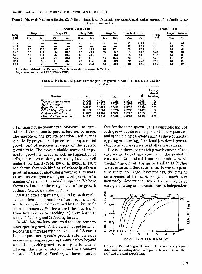
Figure 8 shows posthatch growth curves of thesardine as 1) extrapolated from the prehatchcurves and 2) obtained from posthatch data. Al­though the curves are quite similar at highertemperatures, differences in the lower tempera­ture range are large. Nevertheless, the time todevelopment of the functional jaw is much moreaccurately determined from the extrapolatedcurve, indicating an intrinsic process independent

EE 1.0 13' II'

!!! 5.97

ui ;/

0.9 , ,; E

'", ,

E,.- .-

E ,, :I:E 0.8 ,, I-,, c>, Z:I: ,, WI- 0.7 , ...Jc> ,zw 3.73...J

8 10 12 14

DAYS FROM FERTILIZATION

FIGURE 8.-Posthatch growth curves of the northern anchovy.Solid lines are extrapolated from prehatch curve. Broken linesare fitted to actual growth data.

619

of actual realized size. Comparison of the ex­trapolated curves for the sardine and anchovy,Figures 5 and 7, shows that for the same temper­ature and relative to the asymptotic size, hatchingoccurs later for the anchovy, but jaw developmentand first feeding occur at about the same time.

In summary, each growth cycle may be repre­sented by an equation of the form

with aT = a"e m(l- ('·{iT)

FISHERY BULLETIN: VOL. 74, NO.3

ACKNOWLEDGMENTS

We express our appreciation to David Kramerand Pete Paloma of the National Marine FisheriesService for making unpublished data available tous, to Michel Coirat for her diligent efforts in thelaboratory, to Lorraine Downing for her typingskill and patience with mathematical formulae,and to John R. Hunter for his advice on this work.Special thanks are due to Fishery Bulletinreviewers for checking our mathematics and forconstructive criticism of the manuscript.

or

with

when a temperature optimum exists. The timerequired to attain a given size S is

ts = In [K -ln~SlLoJ laT

which has the same form as the original equation.Most of the data available were from studies of

two species, Sardinops sagax and Engraulis mor­dax, so that generalizations must be made withcaution. Nevertheless, incubation times for sever­al other species fit the model well.

Finally, it seems worthwhile to repeat thatevery growth problem becomes at last a specificone depending on many factors known or un­known, measureable or not. For example, time offertilization will often not be known and agedeterminations will be inexact. Further, Hunterand Lenarz7 have shown that egg size is a mea­surable and probably important factor in growthand survival of anchovy larvae. For feeding larvae,the quantity and quality of food is critical. Eggsize appears to affect growth by a simple scalefactor, all events being shifted up or down inproportion to the egg size. Variation in food mayresult in many "artificial" cycles when nutritionaland caloric requirements are not met. Neverthe­less, it seems clear that at least the early growth ofmany fishes may be described in terms of genet­ically determined but dynamically changinggrowth rates as defined by the Laird-Gompertzgrowth function.

'Hunter, J., and W. Lenarz. 1974. A discussion on the adaptivevalues of variation of fish egg sizes. Unpubl. manuscr., 7 p.Southwest Fisheries Center, Tiburon Laboratory, NationalMarine Fisheries Service, NOAA, Tiburon, CA 94920.

620

LITERATURE CITED

ACTON, F. S.1959. Analysis of straight-line data. John Wiley and Sons,

Inc., N.Y., 267 p.AHLSTROM, E. H.

1943. Studies on the Pacific pilchard or sardine (Sardilwpscacrlllca). 4.-Influence of temperature on the rate ofdevelopment of pilchard eggs in nature. U.S. Fish Wildl.Serv., Spec. Sci. Rep. 23, 26 p.

BEVERTON, R. J. H., AND S. J. HOLT.

1957. On the dynamics of exploited fish populations. Fish.Invest. Minist. Agric., Fish. Food (G.B.), Ser. II, 19, 533 p.

Box, G. E. P., AND G. M. JENKINS.

1970. Time series analysis forecasting and control. Holden­Day, San Franc., 553 p.

CHAPMAN, D. G.1961. Statistical problems in the dynamics of exploited

fisheries populations. Proc. Fourth Berkeley Symposiumon Mathematical Statistics and Probability 4:153-168.

CONWAY, G. R., N. R. GLASS, AND J. C. WILCOX.

1970. Fitting nonlinear models to biological data by Mar­quardt's algorithm. Ecology 51:503-507.

FARRIS, D. A.

1959. A change in the early growth rates of four larvalmarine fishes. Limnol. Oceanogr. 4:29-36.

HALO, A.1952. Statistical theory with engineering applications. John

Wiley and Sons, Inc., N.Y., 783 p.KRAMER, D., AND J. ZWEIFEL.

1970. Growth of anchovy larvae (En,graulis rnordax Girard)in the laboratory as influenced by temperature. Calif.Coop. Oceanic Fish. Invest. Rep. 14:84-87.

LAIRD, A. K.

1964. Dynamics of tumor growth. Br. J. Cancer 18:490-502.1965a. Dynamics of relative growth. Growth 29:249-263.1965b. Dynamics of tumor growth: Comparison of growth

rates and extrapolation of growth curve to one cell. Br. J.Cancer 19:278-291.

1966a. Dynamics of embryonic growth. Growth 30:263-275.1966b. Postnatal growth of birds and mammals. Growth

30:349-363.1967. Evolution of the human growth curve. Growth

31:345-355.LAIRD, A. K., A. D. BARTON, AND S. A. TYLER.

1968. Growth and time: An interpretation of allometry.Growth 32:347-354.

LAIRD, A. K., S. A. TYLER, AND A. D. BARTON.

1965. Dynamics of normal growth. Growth 29:233-248.

ZWEIFEL and LASKER: PREHATCH AND POSTHATCH GROWTH OF FISHES

LASKER, R.

1964. An experimental study of the effect of temperature onthe incubation time, development, and growth of Pacificsardine embryos and larvae. Copeia 1964:399-405.

1970. Utilization of zooplankton energy by a Pacific sardinepopulation in the California Current. In J. H. Steele(editor), Marine food chain, p. 265-284. Oliver and Boyd,Edinb.

LASKER, R., H. M. FEDER, G. H. THEILACKER, AND R. C. MAY.

1970. Feeding, growth, and survival of Engraulis 1I!rmlaxlarVae reared in the laboratory. Mar. BioI. (Berl:)5:345-353.

LEONG, R.1971. Induced spawning of the northern anchovy, Engraulis

nwrdax Girard. Fish. Bull., U.S. 69:357-360.MAY, R. C.

1971. Effects of delayed initial feeding on larvae of thegrunion, LeI/res/lies /emlis (Ayres). Fish. Bull., U.S.69:411-425.

RICHARDS, F. J.1959. A flexible growth function for empirical use. J. Exp.

Bot. 10:290-300.STINNER, R. E., A.P. GUTmRREZ, AND G. D. BUTL~;Il, JIl.

1974. An algorithm fortemperature-dependent growth ratesimulation. Can. Entomol. 106:519-524.

TAYLOIl, C. C.1962. Growth equations with metabolic parameters. J.

Cons. 27:270-286.THOMPSON, D'ARCY WENTWORTH.

1942. On growth and form. 2nd ed. Cambridge Univ. Press,464 p.

VON BEIlTALANFFY , L.1938. A quantitative theory of organic growth (inquiries on

growth laws. 11). Human BioI. 10:181-213.WATANABE, T.

1970. Morphology and ecology of early stages of life inJapanese common mackerel, Scornber japonicns Houttuyn,with special reference to fluctuation of population. [InEngl. and J ap.] Bull. Tokai Reg. Fish. Res. Lab. 62, 283 p.

APPENDIX

InF = InFo + A[l- Exp(-o:t)]/o:

blnF- = [1- Exp(-o:t)]/o:A

blnF- = A[(o:t + 1) Exp(-o:t) - 1]/0:2

0:

For a two-cycle curve with the second cycle begin­ning at t = t* the equations are:

InF = InFo + A[1- Exp(o:LlI)]/o:

+ B[l- Exp(-{1Ll2)]/{1

b~n; = [1- Exp(-{1Ll2)]/,8blnF ={1[({1Ll2 + 1) Exp(-{1Ll2) _ 1]/{12

tI/3

FORTRAN programs are available for fittingsingle-cycle, temperature-dependent and multi­cycle, temperature-dependent curves at SWFC.

The estimation procedure of Conway et aJ.(1970) is a least squares procedure which requiresonly the definition of the functional relationshipand the first derivative with respect to eachparameter. Although not stated explicitly, con­stant variance is assumed and, hence, the loga­rithmic form will be used throughout. For a sin­gle-cycle Laird-Gompertz curve the equations areas follows:

where III = MIN (t, t*)

Ll 2 = MAX (t - t* ,0).

621