Preference-Based Search and Multi-Criteria Optimization

Annals of Operations Research 130, 75–115, 2004 2004 Kluwer Academic Publishers. Manufactured in The Netherlands.

Preference-Based Search and Multi-CriteriaOptimization ∗

ULRICH JUNKER [email protected], 1681, route des Dolines, F-06560 Valbonne, France

Abstract. Many real-world AI problems (e.g., in configuration) are weakly constrained, thus requiring amechanism for characterizing and finding the preferred solutions. Preference-based search (PBS) exploitspreferences between decisions to focus search to preferred solutions, but does not efficiently treat prefer-ences on global criteria such as the total price or quality of a configuration. We generalize PBS to computebalanced, extreme, and Pareto-optimal solutions for general CSPs, thus handling preferences on and be-tween multiple criteria. A master-PBS selects criteria based on trade-offs and preferences and passes themas an optimization objective to a sub-PBS that performs a constraint-based Branch-and-Bound search. Weproject the preferences of the selected criterion to the search decisions to provide a search heuristic and toreduce search effort, thus giving the criterion a high impact on the search. The resulting method will beparticularly effective for CSPs with large domains that arise if configuration catalogues are large.

Keywords: preferences, nonmonotonic reasoning, constraint satisfaction, multi-criteria optimization,search

Introduction

In this paper, we consider combinatorial problems that are weakly constrained and thatlack a clear global optimization objective. Many real-world AI problems have these char-acteristics: examples can be found in configuration, design, diagnosis, but also in tempo-ral reasoning and scheduling. An example for configuration is a vacation adviser systemthat chooses vacation destinations from a potentially very large catalogue. User require-ments (e.g., about desired vacation activities such as wind-surfing, canyoning), compat-ibility constraints between different destinations, and global ‘resource’ constraints (e.g.,on price) usually have a large set of possible solutions. In spite of this, most of the so-lutions will be discarded as long as more interesting solutions are possible. Preferenceson different choices and criteria are an adequate way to characterize the interesting so-lutions. For example, the user may prefer Hawaii to Florida for doing wind-surfing orprefer cheaper vacations in general.

Different methods for representing and treating preferences have been developed indifferent disciplines. In AI, preferences are often treated in a qualitative way and specifyan order between hypotheses, default rules, or decisions. Examples for this have beenelaborated in nonmonotonic reasoning (Brewka, 1989; Delgrande and Schaub, 2000)

∗ Previous versions of this article have been presented at CP-AI-OR’02 and AAAI-02.

76 JUNKER

and constraint satisfaction (Junker, 2000). Here, preferences can be represented by apredicate or a constraint, which allows complex preference statements (e.g., dynamicpreferences, soft preferences, meta-preferences and so on). Furthermore, preferencesbetween search decisions also allow us to express search heuristics and to reduce searcheffort for certain kinds of scheduling problems (Junker, 2000).

In our vacation adviser example, the basic decisions consist of choosing one (orseveral) destinations and we can thus express preferences between individual destina-tions. However, the user preferences are usually formulated on global criteria, such asthe total price, quality, and distance, which are defined in terms of the prices, qualities,and distances of all the chosen destinations. We thus obtain a multi-criteria optimizationproblem.

We could try to apply the preference-based search (Junker, 2000) by choosing thevalues of the different criteria before choosing the destinations. However, this methodhas severe draw-backs:

1. Choosing the value of a global criterion highly constrains the remaining search prob-lem and usually leads to thrashing behaviour.

2. The different criteria are minimized in a strict order. We get solutions that are optimalw.r.t. some lexicographic order, but none that represents compromises between thedifferent criteria. For example, the system may propose a cheap vacation of badquality and an expensive vacation of good quality, but no compromise between priceand quality.

Hence, a naive application of preferences between decisions to multi-criteria opti-mization problems can lead to thrashing and lacks a balancing mechanism.

Multi-criteria optimization (MCO) avoids those problems. Operations researchprovides different methods for solving a multi-criteria optimization problem. For ex-ample, the problem can be mapped to a single or to a sequence of single-criterion op-timization problems which are then solved by traditional methods. Furthermore, thereare several notions of optimality such as Pareto-optimality, lexicographic optimality,and lexicographic max-order optimality. A recent overview of this large research fieldof multi-criteria optimization can be found in (Ehrgott and Gandibleux, 2000). Basedon these methods, we can thus determine ‘extreme solutions’, where some criteria isfavoured over other criteria, as well as ‘balanced solutions’, where the different crite-ria are as close together as possible and which represent compromises. This balancingrequires that the different criteria are comparable, which is usually achieved by a stan-dardization method. The balancing is not achieved by weighted sums of the differentcriteria, but by a new lexicographic approach that has been studied by different authors(cf. Behringer, 1981; Ehrgott, 1997). According to this approach, we have to proceed asfollows in order to find a compromise between a good price and a good quality: we firstminimize the maximum between (standardized versions of) price and quality, fix one ofthe criteria (e.g., the standardized quality) at the resulting minimum, and then minimizethe other criterion (e.g., the price).

PREFERENCE-BASED SEARCH AND MULTI-CRITERIA OPTIMIZATION 77

In this paper, we will develop a modified version of preference-based search thatsolves a minimization subproblem for finding the best value of a given criterion insteadof trying out the different value assignments. Furthermore, we also show how to computePareto-optimal and balanced solutions with this new version of preference-based search.

Multi-criteria optimization as studied in operations research also has draw-backs.Qualitative preferences as elaborated in AI can help to address the following issues:

1. We would like to state that certain criteria are more important than other criteria with-out choosing a total ranking of the criteria as required by lexicographic optimality.For example, we would like to state a preference between a small price and a highquality on the one hand and a small distance on the other hand, but we would still liketo get a solution where the price is minimized first and a solution where the quality ismaximized first.

2. Multi-criteria optimization specifies preferences on global criteria, but it does nottranslate them to preferences between search decisions. In general, it is not evidenthow to derive a search heuristic automatically from the selected optimization objec-tive. Adequate preferences between search decisions provide such a heuristic andalso allow a preference-based search to be applied to reduce the search effort for thesubproblem.

In order to address the first point, we compare the different notions of optimalsolutions with the different notions of preferred solutions that have been elaborated innonmonotonic reasoning (NMR). There have been two major approaches to treat a strictpartial order between default rules. Geffner and Pearl (1992) and Grosof (1991) liftthis order to a partial order among solutions and consider the solutions that are themost preferred ones with respect to this order. Brewka (1989) chooses a lineariza-tion of the partial order and then compares the solutions lexicographically by usingthe chosen linearization as base order. Each linearization leads to a single preferredsolution. Different preferred solutions can be obtained by choosing different lineariza-tions. In (Junker, 1997), we showed that each preferred solution in the sense of Brewka(B-preferred solution) corresponds to a preferred solution in the sense of Geffner andGrosof (G-preferred solution). In this paper, we adapt these definitions to multi-criteriaoptimization. Instead of a strict partial order between default rules, we introduce twokinds of preferences:

1. Preferences on criteria: for each criterion, we consider a strict partial order betweenits possible values and we seek a best value w.r.t. this order.

2. Preferences between criteria: if a criterion z1 is more important than z2, then anyvalue assignment to z1 is more important than any value assignment to z2.

If no preferences between criteria are given, the Pareto-optimal solutions corre-spond to the G-preferred solutions and the lexicographic-optimal solutions correspond tothe B-preferred solutions. Preferences between criteria can easily be taken into accountby the latter methods. For balanced solutions, we present a variant of Ehrgott’s definition

78 JUNKER

Figure 1. Merging concepts from MCO and NMR.

that additionally respects preferences between criteria and we define preferred solutionsin the style of Ehrgott (E-preferred solutions). Thus, we merge concepts from MCO andNMR as illustrated in figure 1. Since the preference-based search method is dedicated toB-preferred solutions, we develop suitable translations of a multi-criteria optimizationproblem such that the G- and E-preferred solutions of the original problem correspondto the B-preferred solutions of the translations. We thus obtain a system where the usercan express preferences on the criteria and preferences between the criteria and choosebetween extreme solutions, balanced solutions and Pareto-optimal solutions.

The preference-based search method explores the given criteria in different ordersthat are compatible with the preferences between criteria. When preference-based searchselects a criterion, it solves a minimization subproblem to determine the best value forthis criterion. Once this value has been found, preference-based search tries out twodifferent possibilities: either it assigns the best value to the selected criterion or it tries torefute this assignment by optimizing other criteria first. Thus, preference-based searchsets up a sequence of minimization subproblems with changing objectives. These sub-problems can be solved by different methods, for example constraint-based Branch-and-Bound. This method imposes an upper-bound constraint on the objective. Although theupper bound is reduced each time a solution is found, the objective has quite a weakimpact on the search space. In particular, the first solution does not depend at all on theobjective since no upper bound is given yet.

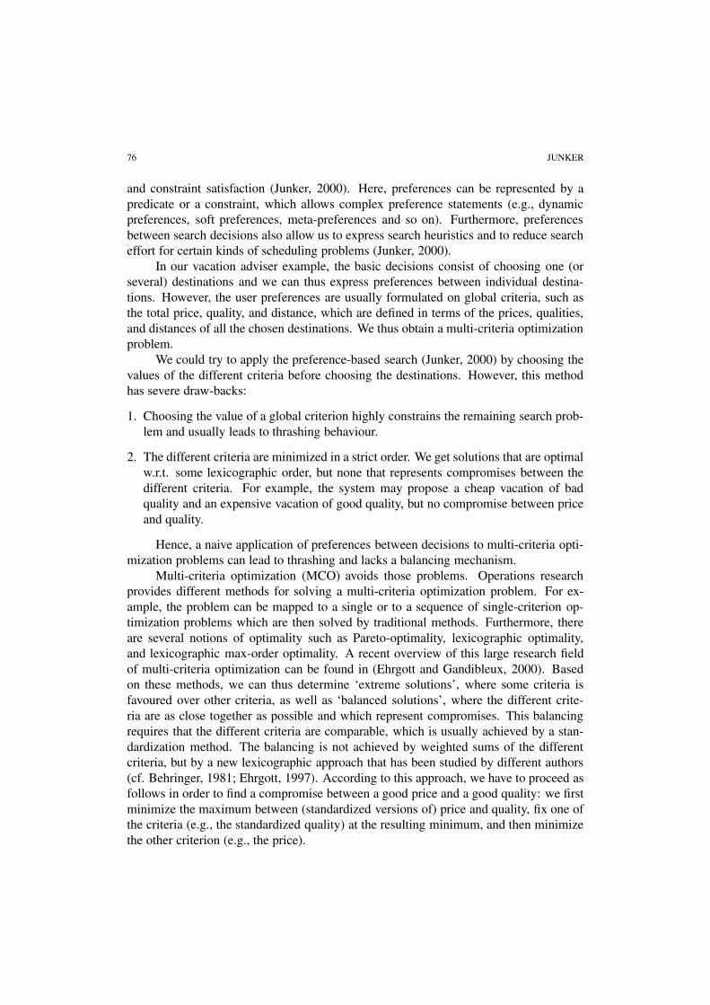
We can improve the search behaviour by projecting the preferences of the selectedcriterion to the search decisions. For example, if we want to minimize the price ofour trip we will choose cheaper hotels first. We will introduce a general method forpreference projection, which we then apply to normal objectives such as sum, min, max,and element constraints. It is important to note that these projected preferences willchange from one subproblem to the other. The projected preferences will be used toguide the search. Depending on the projected preferences, completely different partsof the search space may be explored and, in particular, the first solution depends on thechosen objective. Furthermore, the projected preferences preserve Pareto-optimality andwe can reduce search effort by limiting search to the Pareto-optimal solutions that aredefined by the projected preferences. This can be achieved by a suitable adaption ofpreference-based search to the subproblem as indicated in figure 2.

The paper is organized as follows: we first introduce different notions of optimalityfrom multi-criteria optimization (section 1) and then extend them to cover preferencesbetween criteria (section 2). We then show how these preferences can be formulatedin a general preference programming framework (section 3). After this, we develop


Figure 2. Multiple subsearches driven by Master-PBS.

new versions of preference-based search for computing the different kinds of preferredsolutions (section 4). Finally, we introduce preference projection (section 5). The papersupposes some basic background in optimization as well as constraint programming.

1. Preferences on criteria

We first introduce different notions of optimality from multi-criteria optimization andthen link them to definitions of preferred solutions from nonmonotonic reasoning.

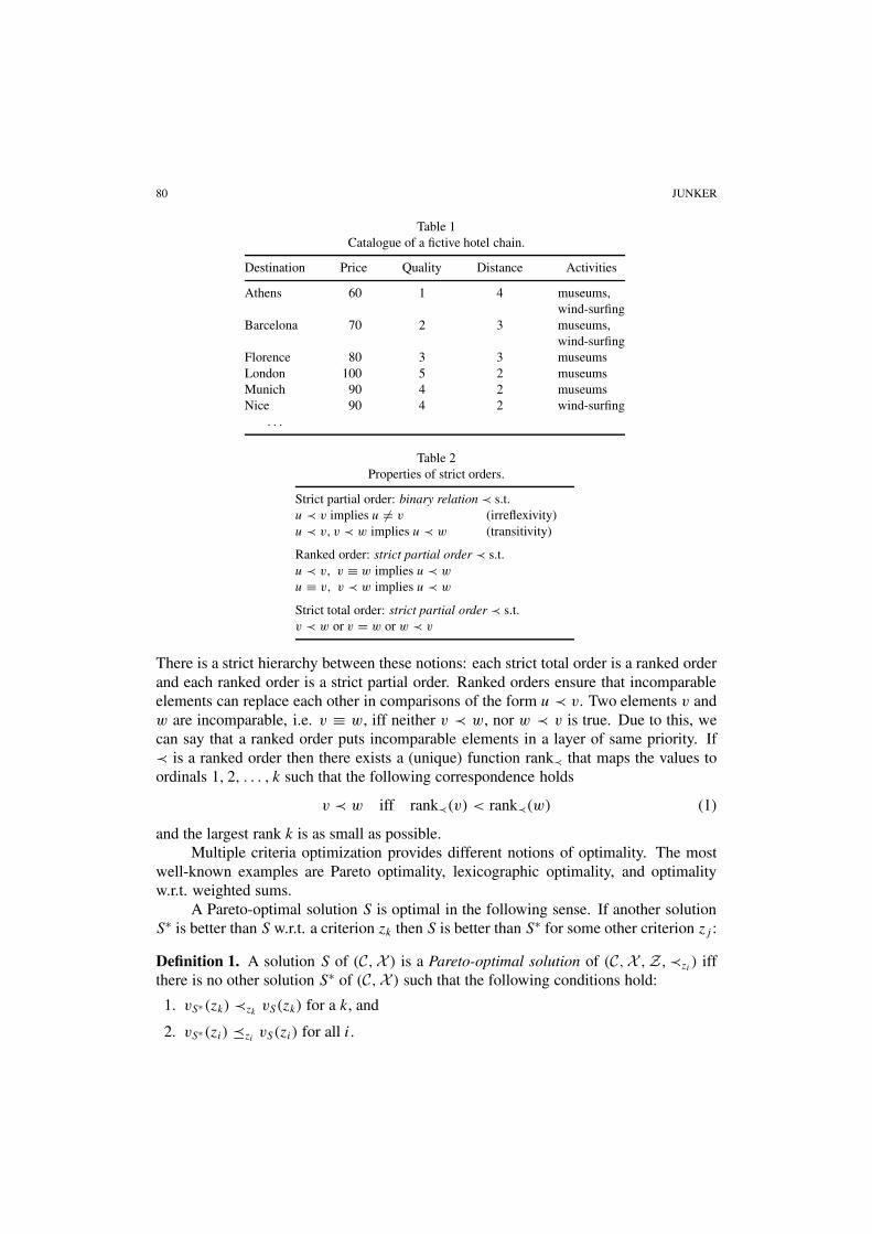
Throughout this paper, we consider combinatorial problems that have the decisionvariables X := (x1, . . . , xm), the criteria Z := (z1, . . . , zn), and the constraints C. Wesuppose that each decision variable xi has a fixed domain D(xi) that is finite and thatspecifies the possible values for xi . In our vacation adviser problem, xi represents the ac-commodation of the ith vacation day. The constraints in C have the form C(x1, . . . , xm).Each constraint symbol C has an associated relation RC . In our example, there may becompatibility constraints (e.g., the destinations of two successive vacation stops shouldbe neighbouring cities) and requirements (e.g., at least one destination should allowwind-surfing and at least one should allow museum visits). Each criterion zi has a de-finition in the form of a functional constraint zi := fi(x1, . . . , xm) and a finite domainD(zi). Examples for criteria are price, quality, and distance (zone). The price is a sumof element constraints:

price :=m∑

i=1

price(xi).

The total quality is defined as the minimum of the individual qualities and the total dis-tance is the maximum of the individual distances. The prices, qualities, and destinationsof the individual accommodations are given by tables such as the catalogue in table 1.

A solution S of (C,X ) is a set of assignments {x1 = v1, . . . , xm = vm} of valuesfrom D(xi) to each xi , such that all constraints in C are satisfied, i.e. (v1, . . . , vm) ∈ RC

for each constraint C(x1, . . . , xm) ∈ C. We write vS(zi) for the value fi(v1, . . . , vm) ofzi in the solution S.

Furthermore, we introduce preferences between the different values for a criterionzi and thus specify a multi-criteria optimization problem. Let ≺zi

⊆ D(zi) × D(zi) be astrict partial order for each zi . For example, we choose < for price and distance and >

for quality. We write u � v iff u ≺ v or u = v.Often, we choose preferences on criteria that satisfy specific properties. Table 2

specifies the properties of strict partial orders, ranked orders, and strict total orders.

80 JUNKER

Table 1Catalogue of a fictive hotel chain.

Destination Price Quality Distance Activities

Athens 60 1 4 museums,wind-surfing

Barcelona 70 2 3 museums,wind-surfing

Florence 80 3 3 museumsLondon 100 5 2 museumsMunich 90 4 2 museumsNice 90 4 2 wind-surfing

. . .

Table 2Properties of strict orders.

Strict partial order: binary relation ≺ s.t.u ≺ v implies u �= v (irreflexivity)u ≺ v, v ≺ w implies u ≺ w (transitivity)

Ranked order: strict partial order ≺ s.t.u ≺ v, v ≡ w implies u ≺ w

u ≡ v, v ≺ w implies u ≺ w

Strict total order: strict partial order ≺ s.t.v ≺ w or v = w or w ≺ v

There is a strict hierarchy between these notions: each strict total order is a ranked orderand each ranked order is a strict partial order. Ranked orders ensure that incomparableelements can replace each other in comparisons of the form u ≺ v. Two elements v andw are incomparable, i.e. v ≡ w, iff neither v ≺ w, nor w ≺ v is true. Due to this, wecan say that a ranked order puts incomparable elements in a layer of same priority. If≺ is a ranked order then there exists a (unique) function rank≺ that maps the values toordinals 1, 2, . . . , k such that the following correspondence holds

v ≺ w iff rank≺(v) < rank≺(w) (1)

and the largest rank k is as small as possible.Multiple criteria optimization provides different notions of optimality. The most

well-known examples are Pareto optimality, lexicographic optimality, and optimalityw.r.t. weighted sums.

A Pareto-optimal solution S is optimal in the following sense. If another solutionS∗ is better than S w.r.t. a criterion zk then S is better than S∗ for some other criterion zj :

Definition 1. A solution S of (C,X ) is a Pareto-optimal solution of (C,X ,Z,≺zi) iff

there is no other solution S∗ of (C,X ) such that the following conditions hold:

1. vS∗(zk) ≺zkvS(zk) for a k, and

2. vS∗(zi) �zivS(zi) for all i.


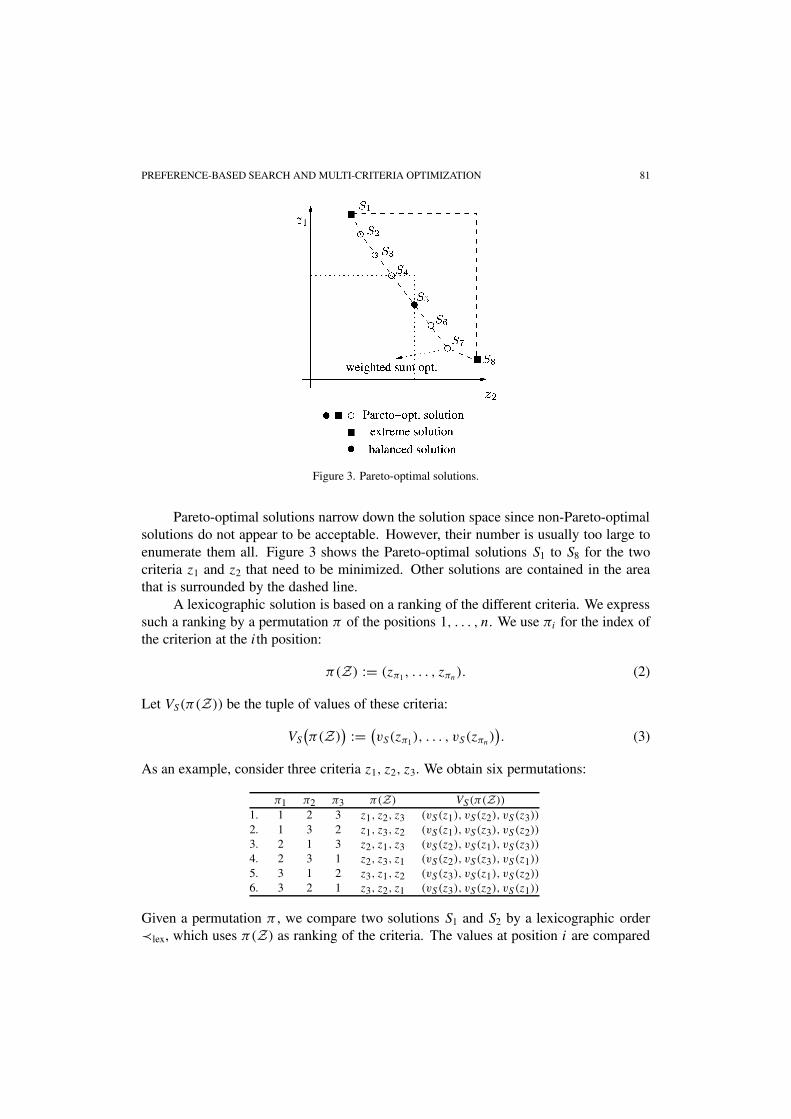
Figure 3. Pareto-optimal solutions.

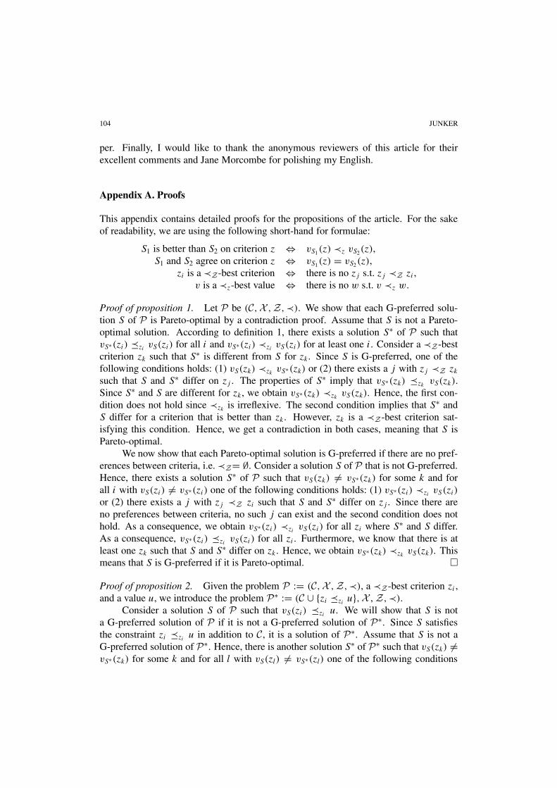
Pareto-optimal solutions narrow down the solution space since non-Pareto-optimalsolutions do not appear to be acceptable. However, their number is usually too large toenumerate them all. Figure 3 shows the Pareto-optimal solutions S1 to S8 for the twocriteria z1 and z2 that need to be minimized. Other solutions are contained in the areathat is surrounded by the dashed line.

A lexicographic solution is based on a ranking of the different criteria. We expresssuch a ranking by a permutation π of the positions 1, . . . , n. We use πi for the index ofthe criterion at the ith position:

π(Z) := (zπ1, . . . , zπn). (2)

Let VS(π(Z)) be the tuple of values of these criteria:

VS

(π(Z)

) := (vS(zπ1), . . . , vS(zπn

)). (3)

As an example, consider three criteria z1, z2, z3. We obtain six permutations:

π1 π2 π3 π(Z) VS(π(Z))

1. 1 2 3 z1, z2, z3 (vS(z1), vS(z2), vS (z3))

2. 1 3 2 z1, z3, z2 (vS(z1), vS(z3), vS (z2))

3. 2 1 3 z2, z1, z3 (vS(z2), vS(z1), vS (z3))

4. 2 3 1 z2, z3, z1 (vS(z2), vS(z3), vS (z1))

5. 3 1 2 z3, z1, z2 (vS(z3), vS(z1), vS (z2))

6. 3 2 1 z3, z2, z1 (vS(z3), vS(z2), vS (z1))

Given a permutation π , we compare two solutions S1 and S2 by a lexicographic order≺lex, which uses π(Z) as ranking of the criteria. The values at position i are compared

82 JUNKER

w.r.t. the preferences on the criterion ≺zπiat position i. Let VS1(π(Z)) := (v1, . . . , vn)

and VS2(π(Z)) := (w1, . . . , wn), We define

(v1, . . . , vn) ≺πlex (w1, . . . , wn) iff

∃k: vk ≺zπkwk and vi = wi for all i = 1, . . . , k − 1.

(4)

Definition 2. Let π be a permutation of 1, . . . , n. A solution S of (C,X ) is an extremesolution of (C,X ,Z,≺zi

) iff there is no other solution S∗ of (C,X ) s.t. VS∗(π(Z)) ≺πlex

VS(π(Z)).

Different rankings lead to different extreme1 solutions which are all Pareto-optimal. In figure 3, we obtain the extreme solutions S1 where z1 is preferred to z2

and S8 where z2 is preferred to z1. Extreme solutions can be determined by solvinga sequence of single-criterion optimization problems starting with the most importantcriterion.

If we cannot establish a preference order between different criteria then we wouldlike to be able to find compromises between them. Although weighted sums (with equalweights) are often used to achieve those compromises, they do not necessarily producethe most balanced solutions. If we choose the same weights for z1 and z2, we obtain S7

as the optimal solution. Furthermore, if we slightly increase the weight of z1 the optimalsolution jumps from S7 to S2. Hence, weighted sums, despite their frequent use, do notappear a good method for balancing.

In (Ehrgott, 1997), Ehrgott uses lexicographic max-orderings to determine optimalsolutions. In this approach, values of different criteria need to be comparable. For thispurpose, we assume that the criteria zi have a common domain D and that the preferenceorders ≺zi

of the different criteria are equal to a strict total order <D. This usuallyrequires some scaling or standardization of the different criteria. We also introduce thereverse order >D which satisfies zi >D zj iff zj <D zi . When comparing two solutionsS1 and S2, the values of the criteria in each solution are first sorted w.r.t. the order >D.The sorted tuples are then compared by a lexicographic order ≺lex. It is important to notethat this sorting can lead to different permutations of the criteria if different solutions areconsidered. We describe the sorting by a permutation ρS that depends on a given solutionS and that satisfies two conditions:

1. ρS sorts the criteria in a decreasing order: if vS(zρSi) >D vS(zρS

j) then i < j .

2. ρS does not change the order if two criteria have the same value: if i < j andvS(zi) = vS(zj ) then ρS

i < ρSj .

Definition 3. A solution S of (C,X ) is a balanced solution of (C,X ,Z,<D) iff thereis no other solution S∗ of (C,X ) s.t. VS∗(ρS∗

(Z)) ≺lex VS(ρS(Z)).

Balanced solutions are Pareto-optimal and they are those Pareto-optimal solutionswhere the different criteria are as close together as possible. In the example of figure 3,


we obtain S5 as balanced solution. According to Ehrgott, it can be determined as follows:first max(z1, z2) is minimized, i.e. max(z1, z2) is used as objective2 of the constraintsatisfaction problem (C,X ). If m is the resulting optimum, the constraint max(z1, z2) =m is added before min(z1, z2) is minimized. Balanced solutions can thus be determinedby solving a sequence of single-criterion optimization problems.

2. Preferences between criteria

If many criteria are given it is natural to specify preferences between different criteria aswell. For example, we would like to specify that a (small) price is more important thana (short) distance without specifying anything about the quality. We therefore introducepreferences between criteria in the form of a strict partial order ≺Z ⊆ Z × Z . Thesepreferences express a notion of relative importance and it is natural to require that thisnotion is transitive and irreflexive.

Preferences on criteria and between criteria can be aggregated to preferences be-tween assignments of the form zi = v. Let ≺ be the smallest relation satisfying thefollowing two conditions: 1. If u ≺zi

v then (zi = u) ≺ (zi = v) and 2. If zi ≺Z zj then(zi = u) ≺ (zj = v) for all u, v. Hence, if a criteria zi is more important than zj , thenany assignment to zi is more important than any assignment to zj . In general, we couldalso have preferences between individual value assignments of different criteria. In thispaper, we simplified the structure of the preferences in order to keep the presentationsimple.

In nonmonotonic reasoning, those preferences ≺ between assignments can be usedin two different ways:

1. as specification of a preference order between solutions,

2. as (incomplete) specification of a total order (or ranking) between all assignments,which is in turn used to define a lexicographic order between solutions.

The Ceteris–Paribus preferences (Boutilier et al., 1997) and the G-preferred solu-tions of (Grosof, 1991; Geffner and Pearl, 1992) follow the first approach, whereas thesecond approach leads to the B-preferred solutions of (Brewka, 1989; Junker, 1997). Wewill now adapt the definitions in (Junker, 1997) to the specific preference structure ofthis paper.

2.1. Generalizing extreme solutions

In the definition of lexicographic optimal solutions, a single ranking of the given criteriais considered. In the definition of B-preferred solutions, we consider all rankings thatrespect the given preferences between the criteria. The following definition has beenadapted from (Brewka, 1989; Junker, 1997) to our specific preference structure:

84 JUNKER

(a) (b)

Figure 4. Preferred solutions.

Definition 4. A solution S of (C,X ) is a B-preferred solution of (C,X ,Z,≺) if thereexists a permutation π such that (1) π respects ≺Z (i.e. zπi

≺Z zπjimplies i < j )

and (2) there is no other solution S∗ of (C,X ) satisfying VS∗(π(Z)) ≺πlex VS(π(Z)).

The B-preferred solution for π can be computed by solving a sequence of mini-mization problems if all ≺zi

are ranked orders. Let C0 := C and

Ci := Ci−1 ∪ {zπi= m},

where

m = min≺zπi

{vS(zπi

) | S is a solution of (Ci−1,X )}.

Each solution of the resulting set Cn is a B-preferred solution and each B-preferred so-lution is a solution of a set Cn of some permutation π . Figure 4 shows different kindsof preferred solutions for three criteria z1, z2, z3 that are all minimized and that respectthe preferences z1 ≺Z z3 and z2 ≺Z z3. The B-preferred solutions are S1, S8 (cf. fig-ure 4(b)). Each B-preferred solution corresponds to an extreme solution. If there areno preferences between criteria, each extreme solution corresponds to some B-preferredsolution.

If there are preferences between criteria certain extreme solutions may not be B-preferred. For example, in figure 4(a), S15 is an extreme solution, which is obtained iffirst the distance z3 is minimized and then the price z1. However, this ranking of thecriteria does not respect the given preferences.


2.2. Generalizing Pareto-optimal solutions

Adapting the G-preferred solutions of (Junker, 1997) to the specific preference structureyields the following definition.

Definition 5. A solution S of (C,X ) is a G-preferred solution of (C,X ,Z,≺) if thereis no other solution S∗ of (C,X ) such that vS(zk) �= vS∗(zk) for some k and all i withvS(zi) �= vS∗(zi) satisfy at least one of the following conditions: (1) vS∗(zi) ≺zi

vS(zi)

or (2) there exists a j s.t. zj ≺Z zi and vS∗(zj ) �= vS(zj ).

A G-preferred solution S is optimal in the following sense. If another solutionS∗ is better than S w.r.t. a criterion zi then there exists a more important criterion zj

such that S and S∗ differ on zj . Then either S is better than S∗ on zj or another crite-rion zk exists, such that S and S∗ differ on zk. We cannot repeat this argumentation aninfinite number of times since ≺Z does not have infinite descending chains due to thefiniteness of Z . Hence, we finally end up with a criterion zk∗ that is more importantthan zi and for which S is better than S∗. Hence, a criterion of a G-preferred solutioncan become worse if a more important criterion is improved. In figure 4(b), S1 to S8

are G-preferred if z1 ≺Z z3 and z2 ≺Z z3 are given. Each G-preferred solution corre-sponds to a Pareto-optimal solution. If there are no preferences between criteria, eachPareto-optimal solution corresponds to some G-preferred solution.

Proposition 1. Let P be (C,X ,Z,≺). If S is a G-preferred solution of P then S is aPareto-optimal solution of P. If S is a Pareto-optimal solution of P and ≺Z= ∅ then S

is a G-preferred solution of P.

However, if there are preferences between criteria, certain Pareto-optimal solutionsS are not G-preferred. There can be a Pareto-optimal solution S that is better than aG-preferred solution S∗ for a criterion zi , but worse for a more important criterion zj

(i.e. zi ≺Z zj ). In this case, the G-preferred solution S∗ is preferred to S meaning thatS is not G-preferred. In figure 4(a), S9 to S17 are Pareto-optimal, but not G-preferred.For example, S9 is not G-preferred since S1 and S9 differ on distance and price. S1 hasa better price than S9 and thus improves S9 w.r.t. this criterion. The fact that S9 has abetter distance than S1 is compensated by the fact that S1 and S9 differ on a criterion thatis more important than the distance, namely the price.

In general, we may get new G-preferred solutions if we add new constraints to ourproblem. However, adding upper bounds to best criteria does not add new G-preferredsolutions. We say z is a ≺Z-best criterion iff there is no z∗ s.t. z∗ ≺Z z:

Proposition 2. Let z be a ≺Z -best criterion. S is a G-preferred solution of (C ∪{z �z u},X ,Z,≺) iff S is a G-preferred solution of (C,X ,Z,≺) and vS(z) �z u.

Although this property appears to be trivial it is not satisfied for the B-preferredsolutions. The property will be essential for computing G-preferred solutions.

86 JUNKER

Furthermore, we can eliminate a best criterion from a problem by assigning a bestvalue to this criterion:

Proposition 3. Let z be a ≺Z -best criterion and v be a ≺z-best value for z. S isa G-preferred solution of (C ∪ {z = v},X ,Z,≺) iff S is a G-preferred solution of(C,X ,Z − {z},≺) and vS(z) = v.

In (Junker, 1997), it has been shown that each B-preferred solution is a G-preferredone, but that the converse is not true in general.

Proposition 4. Let P be (C,X ,Z,≺). Each B-preferred solution of P is also aG-preferred solution of P.

In figure 4(b), S2 to S7 are G-preferred, but not B-preferred. These solutions assigna worse value to z1 than the B-preferred solution S1, but a better value than S8. Similarly,they assign a better value to z2 than S8, but a worse value than S1. It is evident that sucha case cannot arise if each criteria has only two possible values. Hence, we get anequivalence in the following case, where no compromises are possible:

Proposition 5. Let P be (C,X ,Z,≺). If ≺Z is a ranked order and there are no three so-lutions S1, S2, S3 of (C,X ) such that vs1(z) ≺z vs2(z) and vs3(z) ��z vs2(z) for a criterionz then each G-preferred solution of P is also a B-preferred solution of P.

In general, this equivalence does not hold. However, propositions 2 and 5 pointout a possibility for mapping G-preferred solutions to B-preferred solutions if the order≺Z is ranked. The basic idea is to replace the original criteria by binary criteria that aresatisfied if the original criteria are smaller or equal to an upper bound.

Let z be a criterion in Z and let v be a possible value for z. We introduce a binarycriterion uz,v which is equal to 1 if and only if the criterion z has a value smaller or equalto v:

uz,v :={

1 if z �z v,

0 otherwise.(5)

Let U be the set of these upper-bound criteria. It is important to note that the value of abinary criterion uz,v in a solution S is entirely determined by the value of the criterionz in S. Hence, if we know the values of the criteria in a G-preferred solution, we candetermine the values of the binary criteria. Vice versa, if we know the values of thebinary criteria, we can determine the values of the original criteria: vS(z) is equal to the≺z-smallest value w such that vS(uz,w) is equal to one. We can thus replace the set oforiginal criteria Z by U in the translation of the original problem.

We maximize each uz,v, which is expressed by the following preferences on thebinary values:

1 ≺′uz,v

0. (6)


The preferences between the criteria Z are mapped to corresponding preferencesbetween the criteria U . Given two criteria zi and zj the following correspondence holdsfor all upper bounds ui and uj :

zi ≺Z zj implies uzi ,vi≺′

U uzj ,vj. (7)

If the order ≺Z is ranked then ≺′U is ranked as well. We then call the resulting problem

(C,X ,U ,≺′) the bound-translation of (C,X ,Z,≺).The G-preferred solutions are preserved by this translation.

Proposition 6. Let P be (C,X ,Z,≺). S is a G-preferred solution of P iff S is aG-preferred solution of the bound-translation of P.

The bound-translation matches the conditions of proposition 5 since all criteria inU are binary and since we suppose that ≺Z is ranked. Hence, the G-preferred solutionscorrespond to the B-preferred solutions of the bound-translation:

Theorem 1. Let P be (C,X ,Z,≺) and ≺Z be a ranked order. S is a G-preferred solu-tion of P iff S is a B-preferred solution of the bound-translation of P.

If the order ≺Z is not ranked, then the bound-translation is not sufficient to estab-lish a correspondence between B- and G-preferred solution. Future work is needed toaddress this more general case.

2.3. Generalizing balanced solutions

So far, we simply adapted existing notions of preferred solutions to our preference struc-ture and related them to well-known notions of optimality. We now introduce a new kindof preferred solution that generalizes the balanced solutions. We want to be able to bal-ance certain criteria, e.g., the price and the quality, but prefer these two criteria to othercriteria such as the distance. Hence, we limit the balancing to certain groups of criteriainstead of finding a compromise between all criteria. For this purpose, we partition Zinto mutually disjoint sets G1, . . . ,Gk of criteria. Given a criterion z, we also denote itsgroup by G(z). The criteria in a single group Gi will be balanced. The groups them-selves are handled by using a lexicographic approach. Thus, we can treat preferencesbetween different groups, but not between different criteria of a single group. Givena strict partial order ≺G between the Gis, we can easily define an order ≺Z betweencriteria: if G1 ≺G G2 and zi ∈ G1, zj ∈ G2 then zi ≺Z zj . Hence, the preferencesbetween criteria are easy to acquire. If we want to balance several criteria we put theminto the same group. If there are several groups we will determine a balancing for onegroup after another. Preferences between groups constrain the possible orderings of thegroups. The most natural case is obtained if the groups are totally ordered. Otherwise,multiple orders of the groups can be considered.

We now combine definitions 4 and 3. Again, we assume that the preference orders≺zi

of the different criteria are equal to a strict total order <D. As in definition 4, we first

88 JUNKER

choose a global permutation π that respects the preferences between groups. We thenlocally sort the values of each balancing group in a decreasing order. We describe thislocal sorting by a permutation θS that depends on a given solution S and that satisfiesthree conditions:

1. θS can only exchange variables that belong to the same balanced group: G(zi) =G(zθS

i).

2. θS sorts the criteria of each group in a decreasing order: if vS(zθSi) >D vS(zθS

j) and

G(zθSi) = G(zθS

j) then i < j .

3. θS does not change the order if two criteria of the same group have the same value:if i < j , vS(zi) = vS(zj ), and G(zi) = G(zj ) then θS

i < θSj .

Definition 6. A solution S of (C,X ) is an E-preferred solution of (C,X ,Z,≺) if thereexists a permutation π such that (1) π respects ≺Z (i.e. zπi

≺Z zπjimplies i < j )

and (2) there is no other solution S∗ of (C,X ) s.t. VS∗(θS∗(π(Z))) ≺lex VS(θ

S(π(Z))).

The concatenation of the two permutations π and θS∗deserves a short explana-

tion. Firstly, we apply π in order to determine an ordering zπ1, . . . , zπnof the criteria

that respects the preferences between criteria. Let us say that this ordering is equal top1, . . . , pn, i.e. let pi be equal to zπi

. Secondly, we apply θS∗to p1, . . . , pn result-

ing in the ordering pθS∗1

, . . . , pθS∗n

. It is now easy to see that VS(θS(π(Z))) is the tuple

(vS(zπθS1), . . . , vS(zπ

θSn

)).

In figure 4(b), S11 and S12 are balanced solutions w.r.t. the standardized versionsof price, quality, and distance. This notion does not take into account that the distanceis less important than price and quality (z1 ≺Z z3 and z2 ≺Z z3). If we determine theE-preferred solutions, we consider two groups. The more important group contains theprice and quality, whereas the second group contains the distance. In order to obtainthe E-preferred solution S5, we first compute a balanced solution of group 1 and thenminimize the single criterion of group 2. In this case, neither the balanced solutionsare E-preferred, nor the E-preferred solutions are balanced. However, if there is only asingle group, E-preferred solutions coincide with balanced solutions.

Interestingly, we can map E-preferred solutions to B-preferred solutions if weintroduce suitable variables and preferences. We explain the idea for three criteriaZ3 := {z1, z2, z3} and we suppose that the common strict total order <D is the increasingorder on integers, meaning that all three criteria are minimized. The first step consistsin minimizing the criterion that has the worst value in a solution. For this purpose, weintroduce a new criterion

y3 := max(z1, z2, z3) (8)

by using a max-expression.3 Given the best value v3 for y3, we then know that at leastone criterion zk has the value v3 in a preferred solution S and that the other criteria inZ2 := {z1, z2, z3} − {zk} have the same or a better value. We can further compare the


remaining solutions by comparing the values of the criteria in Z2 after setting y3 to v3.We therefore minimize the maximum of the criteria in Z2. We can do this althoughwe do not know zk and the elements of Z2. The trick is to consider all possibilities forZ2, namely {z1, z2}, {z1, z3}, and {z2, z3}. We determine the maximum of each of thesecombinations, namely max(z1, z2), max(z1, z3), max(z2, z3), and distinguish two cases:

1. If zk is in a set {zi, zj } of two criteria then max(zi, zj ) has the value v3 in a solution.

2. If zk is not a set {zi, zj } of two criteria then this set is equal to Z2 and max(zi, zj )

corresponds to our objective, which has a value smaller or equal to v3.

We can thus prove that minimizing

y2 := min(max(z1, z2), max(z1, z3), max(z2, z3)

)(9)

determines the best value v2 of the second worst criterion in a solution. After assigningv2 to y2, we minimize

y1 := min(z1, z2, z3) (10)

in order to find the best value v1 for the third worst criterion (i.e. the best criterion in thisexample).

We now discuss the general case. For each group G of cardinality nG, we use thefollowing min-max-variables yG,nG

, . . . , yG,1. The criterion yG,i is minimized if the bestvalues of all, but i criteria have been found. Since we do not know which of the criteriaare remaining we determine the maximum of each subset of size i and take the minimumof these maxima as explained above:

yG,i := min<D

{max<D

(X) | X ⊆ G s.t. |X| = i}, (11)

where max<D(X) := max<D

{z | z ∈ X}. The min-max-variables can directly be ex-pressed in a constraint programming language. Due to the exponential size of the expres-sion, this is only feasible for a small number of criteria. For a large number of criteria, anoption for future work is the development of a global constraint. Let Z := {z1, . . . , zn}be the set of all of these min-max-variables. The zi are arranged in an order that pre-serves the group of position i: if the criterion zi belongs to group G then zi also belongsto group G and is equal to yG,j for some j .

We now adapt the preferences ≺ to the new criteria and we denote the result by ≺.The preference order ≺yG,i

of all criteria yG,i is equal to the strict total order <D. Thepreferences ≺Z between the criteria Z satisfy two properties:

1. The following preferences ensure that min-max-variables for larger subsets X aremore important:

yG,i≺Z yG,i−1 for i = nG, . . . , 2. (12)

2. A preference between a group G∗ and a group G can be translated into a preferencebetween the last min–max-variable of G∗ and the first one of G:

yG∗,1≺Z yG,nG. (13)

90 JUNKER

We call the resulting problem (C,X , Z, ≺) the min-max-translation of (C,X ,Z,≺).The E-preferred solutions then correspond to the B-preferred solutions of the trans-

lated criteria and preferences:

Theorem 2. Let P be (C,X ,Z,≺). S is an E-preferred solution of P iff S is aB-preferred solution of the min-max-translation of P.

We have thus established variants of Pareto-optimal, extreme, and balanced solu-tions that take into account preferences between criteria. On the one hand, we gain abetter understanding of the existing preferred solutions by this comparison with notionsfrom multi-criteria optimization. On the other hand, we obtain a balancing mechanismthat fits well into the qualitative preference framework.

3. Preference programming

In the previous section, we defined preferred solutions based on preferences on criteriaand between criteria, but we did not discuss how these preferences can be specified. Forthis purpose, we enhance traditional constraint programming by primitives for statingpreferences. We thus obtain a system of preference programming, which is describedin (Junker and Mailharro, 2003b) in detail. Preference programming has been imple-mented in ILOG JCONFIGURATOR 2.0 (ILOG, 2002) and supports different preference-based problem solving tasks such as searching for a solution guided by preferences,finding a preferred explanation, and satisfying user preferences. Furthermore, JCON-FIGURATOR combines an expressive constraint language with a description logic for de-scribing the taxonomic and partonomic configuration knowledge (Junker and Mailharro,2003a).

In this section, we show how preferences on and between criteria can be specifiedwithin the preference programming framework. In our approach, preferences constrainthe order in which decisions are made. We therefore represent preferences by specialkinds of constraints. Preferences between two criteria (e.g., price and distance) can bestated by the following constraint:

prefer(price, distance);

The strict partial order ≺Z is then defined as the transitive closure of the set of all tuples(zi, zj ) for which prefer(zi, zj ) is given. If the transitive closure is not irreflexive thenthe preference statements are considered inconsistent.

Domain orders ≺zican be specified in a compact way. We represent the increasing

order on integers by minFirst and the decreasing order on integers by maxFirst.Ranked orders can be expressed by assigning a priority to each value and strict partialorders can be formulated by prefer-statements between values (Junker and Mailharro,2003b). A domain order is applied to a criterion by a preferValues-constraint:


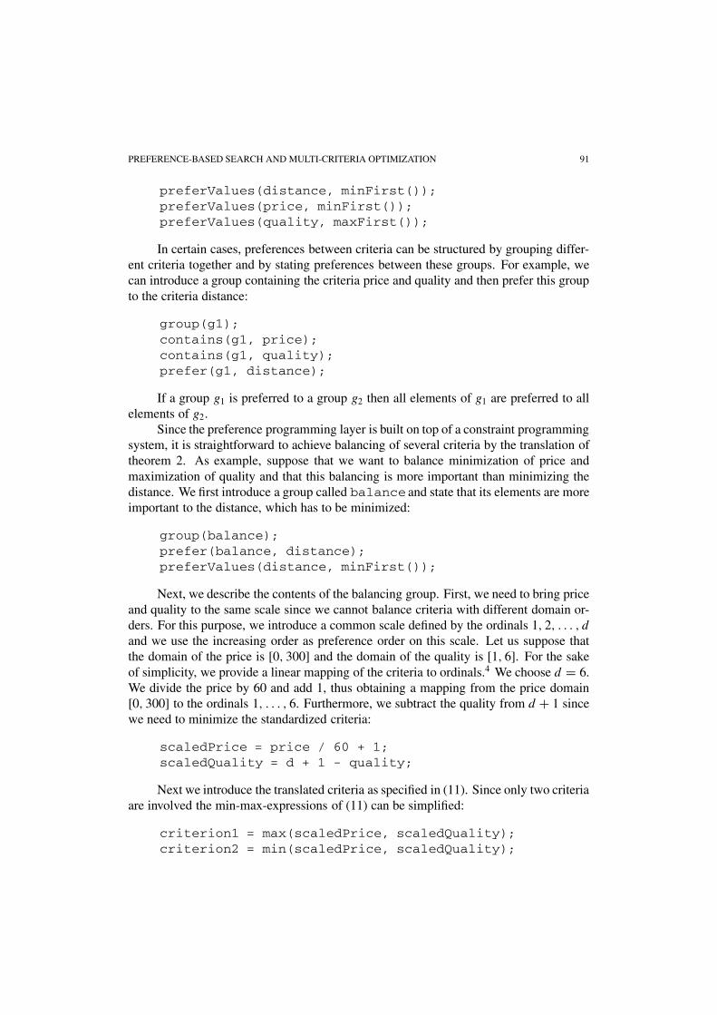
preferValues(distance, minFirst());preferValues(price, minFirst());preferValues(quality, maxFirst());

In certain cases, preferences between criteria can be structured by grouping differ-ent criteria together and by stating preferences between these groups. For example, wecan introduce a group containing the criteria price and quality and then prefer this groupto the criteria distance:

group(g1);contains(g1, price);contains(g1, quality);prefer(g1, distance);

If a group g1 is preferred to a group g2 then all elements of g1 are preferred to allelements of g2.

Since the preference programming layer is built on top of a constraint programmingsystem, it is straightforward to achieve balancing of several criteria by the translation oftheorem 2. As example, suppose that we want to balance minimization of price andmaximization of quality and that this balancing is more important than minimizing thedistance. We first introduce a group called balance and state that its elements are moreimportant to the distance, which has to be minimized:

group(balance);prefer(balance, distance);preferValues(distance, minFirst());

Next, we describe the contents of the balancing group. First, we need to bring priceand quality to the same scale since we cannot balance criteria with different domain or-ders. For this purpose, we introduce a common scale defined by the ordinals 1, 2, . . . , d

and we use the increasing order as preference order on this scale. Let us suppose thatthe domain of the price is [0, 300] and the domain of the quality is [1, 6]. For the sakeof simplicity, we provide a linear mapping of the criteria to ordinals.4 We choose d = 6.We divide the price by 60 and add 1, thus obtaining a mapping from the price domain[0, 300] to the ordinals 1, . . . , 6. Furthermore, we subtract the quality from d + 1 sincewe need to minimize the standardized criteria:

scaledPrice = price / 60 + 1;scaledQuality = d + 1 - quality;

Next we introduce the translated criteria as specified in (11). Since only two criteriaare involved the min-max-expressions of (11) can be simplified:

criterion1 = max(scaledPrice, scaledQuality);criterion2 = min(scaledPrice, scaledQuality);

92 JUNKER

Finally, we add the new criteria to the group balance and specify their domainorders:

contains(balance, criterion1);contains(balance, criterion2);preferValues(criterion1, minFirst());preferValues(criterion2, minFirst());prefer(criterion1, criterion2);

This example shows how balanced solutions can be determined with JCONFIGURATOR

2.0.

4. Preference-based search

We now adapt the preference-based search (PBS) algorithm from (Junker, 2000) to treatpreferences on criteria. PBS was designed as a search algorithm that reduces searcheffort by focusing on preferred choices. If v is a best value for a variable x, PBS eithertries the assignment x = v or tries to refute it by making best assignments for othervariables. PBS abandons a best choice only if such a refutation succeeds. Otherwise, itfails.

We could apply the original PBS to multi-criteria optimization. In this case, PBSwould first choose the values of the criteria before choosing the values of the decisionvariables. However, the assignments to criteria are often very constraining and we easilyget a thrashing behaviour as long as these assignments are not supported by any solu-tion. A better idea is to directly determine the best value of a criterion z by solving aminimization subproblem:

minimize(C, z,≺z) := min{rank≺z

(vS(z)

) | S is a solution of (C,X )}. (14)

In order to obtain a traditional minimization problem, we only consider ranked orders≺zi

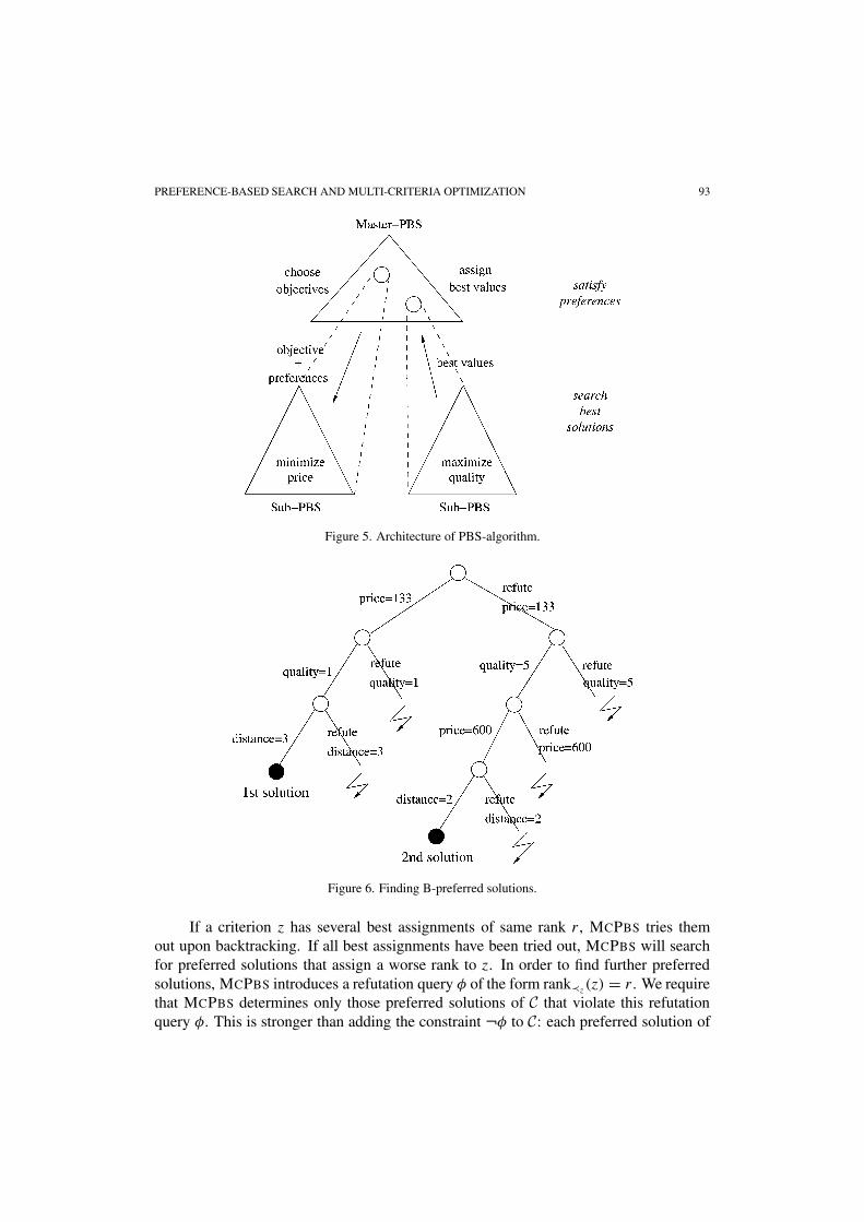
throughout this section.The resulting algorithm is called MCPBS5 and follows the architecture in figure 5.

We explain its basic idea for the example shown in figure 6, where price and qualityare preferred to distance. The algorithm maintains a set U of unexplored criteria, whichis initialized with the set of all criteria (i.e. price, quality, and distance). In each step,the algorithm selects a best criterion z of U (e.g., the price). Instead of trying to as-sign different values to the total price, we determine the cheapest price by solving aminimization subproblem minimize(C, price,<) as explained above. In our example,the cheapest solution has a price of 133. We now add the assignment price = 133 tothe initial set C of constraints. In figure 6, these assignments occur as labels of the leftbranches. We then determine the best quality under this assignment. Once the price andquality have been determined we can determine a distance as well, thus obtaining a firstsolution.


Figure 5. Architecture of PBS-algorithm.

Figure 6. Finding B-preferred solutions.

If a criterion z has several best assignments of same rank r, MCPBS tries themout upon backtracking. If all best assignments have been tried out, MCPBS will searchfor preferred solutions that assign a worse rank to z. In order to find further preferredsolutions, MCPBS introduces a refutation query φ of the form rank≺z

(z) = r. We requirethat MCPBS determines only those preferred solutions of C that violate this refutationquery φ. This is stronger than adding the constraint ¬φ to C: each preferred solution of

94 JUNKER

C that violates φ is a preferred solution of C ∪ {¬φ}, but C ∪ {¬φ} may have preferredsolutions, which are not preferred solutions of C and which must not be determinedby MCPBS.

We say that a refutation query rank≺z(z) = r is refuted if it becomes inconsistent

after assigning values to the unexplored criteria that may precede z. The refutationqueries are added to a set Q. We can remove an element from Q if it has been refutedafter making other assignments.

In our example, the assignment to the distance cannot be refuted since there areno further unexplored criteria. The quality of 1 cannot be refuted since the single non-explored criterion distance cannot precede the quality. However, we can refute the priceof 133 by first maximizing the quality. After this, we can again minimize the price andthe distance, which leads to a new solution as shown in figure 6. This example showsthat refutation queries lead to a change of the exploration order of criteria.

The algorithm cannot select a criterion z if it has a refutation query in Q. Wedenote the set of criteria with refutation queries by

Z(Q) := {z ∈ Z | ∃(rank≺z

(z) = q) ∈ Q}. (15)

When adding a new constraint to C, we use a constraint propagation procedure to reducethe possible values for each criterion z. The reduced domain of z is denoted by domC(z).Different constraint propagation algorithms can be used that maintain different degreesof local consistency. A minimal assumption is to maintain node consistency for unaryconstraints and bound consistency for non-unary constraints. If a criterion has a singlepossible value in domC(z) then MCPBS does not need to try out different assignmentsfor z and can explore it without solving a minimization problem.

The resulting search algorithm is shown in figure 7. For the sake of comprehensi-bility, we present it as a non-deterministic algorithm that uses try-statements as in OPL(van Hentenryck, Perron, and Puget, 2000) to describe the branching. The statement‘try A or B’ performs a simple branching. In the left branch, A is executed, whereasB is executed in the right branch. The statement ‘try A for each v ∈ V ’ creates severalbranches, namely, one for each value in V .

Furthermore, MCPBS uses several subprocedures (see figure 8) that can have dif-ferent implementations and that may make some global updates of the data structuresof MCPBS, such as the addition of new constraints. The subprocedure ISCONSISTENT

checks the consistency of the constraints. The selection of a best criteria is done by theprocedure SELECT. The procedure MINIMIZE determines the best rank for the chosencriterion.

The algorithm maintains a state σ := (C,Q,U) consisting of the set C of con-straints, the set Q of refutation queries, and the set U of unexplored criteria. We say thatS is a B-preferred solution of the state σ iff S is a B-preferred solution of the problemPσ := (C,X , U,≺) and S violates each (rank≺z

(z) = q) in Q. Given a state σ , weconsider the best unexplored criteria

Bσ := {z ∈ U |� ∃z∗ ∈ U : z∗ ≺Z z

}(16)


Figure 7. Algorithm for computing B-preferred solutions.

Figure 8. Subprocedures for extreme solutions.

96 JUNKER

and their best ranks:

rankσ (z) := min{rank≺z

(vS(z)

) | S is a solution of C}. (17)

If the rank rank≺z(v) of a value v is equal to rankσ (z) then there is no solution S that

assigns a better value to z. This means vS(z) ≺z v is not possible in this case.MCPBS is based on the following properties of a state σ :

• Success: If U = ∅ and Q = ∅ then each solution of (C,X ) is a B-preferred solutionof σ .

• Refutation query: Let z ∈ U and q be any value. S is a B-preferred solution of(C,Q∪{rank≺z

(z) = q}, U) iff S is a B-preferred solution of (C,Q,U) and S violatesrank≺z

(z) = q.

• Choice: Let z ∈ Bσ and v be a value having the rank rankσ (z). S is a B-preferredsolution of (C ∪ {z = v}, Q,U −{z}) iff S is a B-preferred solution of (C,Q,U) andS satisfies z = v.

• Refutation: Suppose (rank≺z(z) = q) ∈ Q and q < rankσ (z). Then S is a B-preferred

solution of (C,Q,U) iff S is a B-preferred solution of (C,Q − {rank≺z(z) = q}, U).

• Global fail: If U �= ∅ and for all z ∈ Bσ we have (rank≺z(z) = rankσ (z)) ∈ Q then

(C,Q,U) has no B-preferred solution.

MCPBS has an inner loop and an outer loop. In each iteration of the outer loop, itfirst determines the set B of best criteria. In the inner loop, it either assigns a value toa single criterion z of B or it ensures that each criterion in B has a refutation query forits best rank. In the first case, MCPBS removes z from U and immediately leaves theinner loop. B is updated in the next iteration of the outer loop. In the second case, theconditions of a global fail are satisfied and MCPBS fails (cf. line 18 in figure 7: pleasenote that B ⊆ U holds in the second case, but not in the first case since z from B is nolonger in U ). We are now able to show that MCPBS is correct and complete:

Theorem 3. Suppose that all ≺ziare ranked. Algorithm MCPBS(C,X ,Z,≺) always

terminates. Each successful run returns a set X of constraints, the solutions of which areB-preferred solution of (C,X ,Z,≺) and each such B-preferred solution is the solutionof the result X of exactly one successful run.

MCPBS can solve several minimization subproblems for the same criterion z ifit has a refutation query for z in Q. In the worst case, such a minimization problemis solved each time an assignment is added to C. The number of subproblems can bereduced by keeping previous solutions as supports. Suppose that rank q for criterion z

needs to be refuted. MCPBS determined a solution Sz with rank≺z(vS(z)) = q before

it added the refutation query. We can keep this solution as support for the best rank q

of z. If the refutation query is checked again after adding the constraint � to C, we firsttest whether Sz is a solution of C ∪ �. If yes, then the best rank for z in C ∪ � is q andthe refutation query has not been refuted by the additional constraints. As long as the


supporting solution Sz of the refutation query satisfies all constraints, we do not need tosolve a minimization problem. The subprocedures in figure 8 incorporate supports. Wealso introduce a support S∗ for the consistency check of C. Future work will be devotedto improve the pruning of the search tree by exploiting further properties of refutationqueries and solution supports. For example, we can post a constraint that avoids that Sz

is computed twice and that prunes solutions dominated by Sz as in (Gavanelli, 2002).We analyze the complexity for the case where each criterion z has d possible values

and a strict total order ≺z. In each successful iteration of the inner-loop, the algorithmMCPBS either assigns a value to a criterion or adds a refutation query requiring thatthis assignment will be violated. Hence, each non-deterministic run needs at least O(n)

iterations (where n is the number of criteria) and at most O(n · d) iterations. Sinceeach iteration corresponds to a branching in a search tree, we obtain a search tree witha branching factor of 2 and a maximal depth of O(n · d). Hence, O(2n·d) is an upperbound for the number of search nodes. Furthermore, the number of search states is alsobounded by the number of permutations of criteria, namely, O(n!).

Given the bound-translation of a problem, we can use MCPBS to determine allPareto-optimal solutions. We consider a very simple example involving two criteria a, b

that have both the domain [1, d] and that are both minimized. Suppose that there arethree Pareto-optimal solutions. The first one is vS1(a) = 1, vS1(b) = 5, the secondone is vS2(a) = 2, vS2(b) = 2, and the third one is vS3(a) = 5, vS3(b) = 1. In spiteof the simplicity of the example, we have 2d binary criteria, namely ua,1, . . . , ua,d andub,1, . . . , ub,d . There are no preferences between these binary criteria, but there are log-ical dependencies that can be exploited when running MCPBS on the bound translationand that have a high impact on the form of the search tree. The search tree in figure 9 isobtained by the following observations:

1. If we add the constraint uz,v = 1 to C then constraint propagation reduces the domainsof the criteria uz,w with v ≺z w to 1 meaning that these criteria are skipped byMCPBS in line 13. For example, when adding ua,1 = 1 in the left branch, constraintpropagation deduces that the criteria ua,i+1, . . . , ua,d are all equal to 1 and MCPBS

does not do any branching for them.

2. Let m be the best rank for criterion z. If we add the constraint rank≺z(z) � m to C,

then constraint propagation reduces the domains of the criteria uz,w with rank≺z(w) <

m to 0. For example, ub,1, . . . , ub,4 are all 0 after adding ub,5 = 1 and need not beconsidered.

3. If there is a refutation query uz,v = 1 in Q and w ≺z v, then violating uz,v = 1 willviolate uz,w = 1 as well. Hence, uz,w = 1 needs to be refuted as well in this case. Wetherefore will not select ub,1, . . . , ub,4 when seeking a refutation of ub,5 = 1.

We thus select a binary criterion uz,v with a best bound v for z in order to recon-stitute the search behaviour of MCPBS on the original problem when running it on thebound-translation. Furthermore, we can improve the refutation behaviour by exploitingthe supporting solutions of refutation queries:

98 JUNKER

Figure 9. Determining Pareto-optimal solutions.

1. If there is a refutation query uz,v = 1 in Q and uz,v = 1 is not refuted by C, then thereexists a solution S of C that satisfies uz,v = 1. It also satisfies uz,w = 1 for w �z v.Hence, adding uz,w = 1 to C will not produce a state where uz,v = 1 is refuted. Wetherefore will not select ub,6, . . . , ub,d when seeking a refutation of ub,5 = 1.

2. As a consequence, a refutation query uz,v = 1 in Q cannot be refuted if all binarycriteria in B have the form uz,v′ , i.e. concern the original criterion z. Therefore,ub,5 = 1 cannot be refuted.

3. If a refutation query uz,v = 1 in Q is satisfied by the solution Sz and Sz is a solution ofC, then we select a criterion uz∗,v∗ such that adding uz∗,v∗ = 1 will invalidate Sz Theconstraint z∗ �z v∗ is satisfied by Sz if and only if vSz

(z∗) �z v∗. Hence, uz∗,v∗ =1 invalidates Sz if vSz

(z∗) ��z v∗. We choose a �z-largest value v∗ satisfying thiscondition. For example, we choose ub,4 = 1 to invalidate the support S1 for ua,1 = 1and ub,1 = 1 to invalidate the support S2 for ua,2 = 1.However, if no such criterion z∗ and value v∗ exist then uz,v = 1 cannot be refuted,meaning that the current state has no G-preferred solution. In this case, a failureoccurs.

We have thus seen how solution supports for refutation queries can guide the se-lection of binary criteria and ensure that refutations can be found. Moreover, solutionsupports for refutation queries could be used to do additional propagations and deduc-tions: if there is only one possibility to invalidate a support for a refutation query, thenthis possibility must be true. A detailed elaboration of those rules is a subject of futurework.


Figure 10. Subprocedures for Pareto-optimal solutions.

We now adapt the subprocedures to the bound-translation and incorporate the se-lection rules for the bound translation. The resulting subprocedures are shown in fig-ure 10. Please note that minimization subproblems and solution supports Sz refer to theoriginal criteria z and not to the binary criteria uz,v. These changes ensure that MCPBS

provides an adequate search behaviour for enumerating Pareto-optimal solutions. Fortwo criteria, we get a behaviour that is similar6 to the algorithm of Van Wassenhove andGelders (1980), which determines all Pareto-optimal solutions for bicriteria-problems.On the one hand, we thus derive a well-known algorithm from more basic principles andwe can understand it as a method that deduces bound-constraints from solution supportsof refutation queries. On the other hand, we can understand MCPBS (on the bound-translation) as a method that generalizes the algorithm of Van Wassenhove and Geldersto more than two criteria.

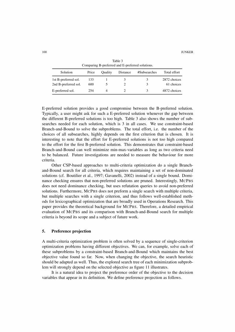
According to theorem 2, we can also use MCPBS to compute balanced solutionsif we apply it to the min-max-translation. Table 3 shows the values of the three criteriaprice, quality, and distance for the two B-preferred solutions and the unique E-preferredsolution, which is determined w.r.t. the two groups G1 := {scaledPrice, scaledQuality}and G2 := {scaledDistance}, where G1 is more important than G2. We see that the

100 JUNKER

Table 3Comparing B-preferred and E-preferred solutions.

Solution Price Quality Distance #Subsearches Total effort

1st B-preferred sol. 133 1 3 3 2872 choices2nd B-preferred sol. 600 5 2 3 61 choices

E-preferred sol. 254 4 2 3 4872 choices

E-preferred solution provides a good compromise between the B-preferred solution.Typically, a user might ask for such a E-preferred solution whenever the gap betweenthe different B-preferred solutions is too high. Table 3 also shows the number of sub-searches needed for each solution, which is 3 in all cases. We use constraint-basedBranch-and-Bound to solve the subproblems. The total effort, i.e. the number of thechoices of all subsearches, highly depends on the first criterion that is chosen. It isinteresting to note that the effort for E-preferred solutions is not too high comparedto the effort for the first B-preferred solution. This demonstrates that constraint-basedBranch-and-Bound can well minimize min-max-variables as long as two criteria needto be balanced. Future investigations are needed to measure the behaviour for morecriteria.

Other CSP-based approaches to multi-criteria optimization do a single Branch-and-Bound search for all criteria, which requires maintaining a set of non-dominatedsolutions (cf. Boutilier et al., 1997; Gavanelli, 2002) instead of a single bound. Domi-nance checking ensures that non-preferred solutions are pruned. Interestingly, MCPBS

does not need dominance checking, but uses refutation queries to avoid non-preferredsolutions. Furthermore, MCPBS does not preform a single search with multiple criteria,but multiple searches with a single criterion, and thus follows well-established meth-ods for lexicographical optimization that are broadly used in Operations Research. Thispaper provides the theoretical background for MCPBS. Therefore, a detailed empiricalevaluation of MCPBS and its comparison with Branch-and-Bound search for multiplecriteria is beyond its scope and a subject of future work.

5. Preference projection

A multi-criteria optimization problem is often solved by a sequence of single-criterionoptimization problems having different objectives. We can, for example, solve each ofthese subproblems by a constraint-based Branch-and-Bound which maintains the bestobjective value found so far. Now, when changing the objective, the search heuristicshould be adapted as well. Thus, the explored search tree of each minimization subprob-lem will strongly depend on the selected objective as figure 11 illustrates.

It is a natural idea to project the preference order of the objective to the decisionvariables that appear in its definition. We define preference projection as follows.


Figure 11. Explored subtree depends on projected preferences.

Definition 7. ≺xkis a projection of ≺zj

via fj (x1, . . . , xm) to xk if and only if thefollowing condition holds for all u1, . . . , um and v1, . . . , vm with ui = vi for i =1, . . . , k − 1, k + 1, . . . , m:

if uk ≺xkvk then fj (u1, . . . , um) �zj

fj (v1, . . . , vm). (18)

Definition 8. ≺x1, . . . ,≺xmis a projection of ≺z1, . . . ,≺zn

via f1, . . . , fn to x1, . . . , xm

if ≺xiis a projection of ≺zj

via fj (x1, . . . , xm) to xi for all i, j .

The projected preferences preserve Pareto-optimality:

Theorem 4. Let ≺x1, . . . ,≺xmbe a projection of ≺z1, . . . ,≺zn

via f1, . . . , fn tox1, . . . , xm. If S is a Pareto-optimal solution w.r.t. the criteria z1, . . . , zn and the prefer-ences ≺z1, . . . ,≺zn

then there exists a solution S∗ that (1) is a Pareto-optimal solutionw.r.t. the criteria x1, . . . , xm and the preferences ≺x1, . . . ,≺xm

and (2) vS∗(zi) = vS(zi)

for all criteria zi .

We give some examples for preference projections satisfying the conditions of de-finition 7:

1. The increasing order < is a projection of < via sum, min, max, and multiplicationwith a positive coefficient.

2. The decreasing order > is a projection of < via a multiplication with a negativecoefficient.

102 JUNKER

Table 4Reduction of search effort by preference projection.

Objective Projection Distance to opt. Effort Effort(1st. sol.) (best sol.) (opt. proof)

minimize no 248% 462 choices 1203 choicesprice yes 24% 251 choices 675 choicesmaximize no 20% 27 choices 27 choicesquality yes 0% 16 choices 16 choices

3. Given an element constraint (i.e. an arbitrary functional constraint) of the form y =f (x) that maps each possible value i of x to a value f (i), the following order ≺x is aprojection of < to x via f (x):

u ≺x v iff f (u) < f (v). (19)

Hence, projecting the increasing or decreasing order on integers via an element con-straint yields a ranked order.

Table 4 shows the impact of preference projection on our vacation adviser prob-lem. We consider the subsearches for B-preferred solutions that are performed for thefirst selected criterion, namely the quality or the price. These criteria are defined bydifferent element constraints and the projected preferences completely differ dependingon the selected objective. If we want to minimize the price, the projected preferencesensure that cheaper hotels are selected first for each vacation stop. If we want to max-imize the quality, the projected preferences will favour hotels of better quality in eachstop.

In this example, preference projection helps to reduce the number of choicesaround 45%. More importantly, it improves the degree of optimality of the first solu-tion. If no preference projection is used the first solution has a distance of 248% to thebest price and a distance of 20% to the best quality. If preference projection is used, thefirst solution depends on the chosen objective. If price is minimized first the distanceto the best price reduces from 248% to 24%. If quality is maximized first the distanceto the best quality reduces from 20% to 0%. Hence, these two solutions are completelydifferent. Since the problem is weakly constrained, the first solutions are found rapidly,meaning that different trade-offs can indeed be produced in a small time frame if prefer-ence projection is used.

This shows that preference projection is of high importance for interactive con-figuration problems where time is limited. If only a single solution can be determinedby each subsearch, standard constraint-based Branch-and-Bound will always return thesame solution independent of the selected objective. In this case, preference projectionensures that the selected objective is taken into account and that different solutions aredetermined. Again, this is important for interactive configuration, where we want todetermine several solutions of different characteristics in a short time frame.


Since extreme and balanced solutions are Pareto-optimal, we can additionally usethe projected preferences to reduce search effort when solving a subproblem. For thispurpose, we can apply the algorithm MCPBS to the decision variables x1, . . . , xm andthe bound-translation. An investigation of the possible gains of this method is a subjectof future work.

6. Conclusion

Although preference-based search (Junker, 2000) provided an interesting technique forreducing search effort based on preferences, it could only take into account preferencesbetween search decisions, was limited to combinatorial problems of a special structure,and did not provide any method for finding compromises in the absence of preferences.In this paper, we have lifted PBS from preferences on decisions to preferences on crite-ria, as they are common in qualitative decision theory (Doyle and Thomason, 1999; Bac-chus and Grove, 1995; Boutilier et al., 1997; Domshlak, Brafman, and Shimony, 2001).We further generalized PBS, such that not only extreme solutions are computed, butalso balanced and Pareto-optimal solutions. Balanced solutions can be computed bya modified lexicographic approach (Ehrgott, 1997), which fits well into a qualitativepreference framework as studied in nonmonotonic reasoning and qualitative decisiontheory.

Our search procedure consists of two modules. A master-PBS explores the criteriain different orders and assigns optimal values to them. The optimal value of a selectedcriterion is determined by a sub-PBS, which performs a constraint-based Branch-and-Bound search through the original problem space (i.e. the different value assignmentsto decision variables). Furthermore, we project the preferences on the selected criterionto preferences between the search decisions, which provides an adapted search heuristicfor the optimization objective and which allows the search effort to be reduced fur-ther. Hence, different regions of the search space will be explored depending on theselected objective. The master-PBS has been implemented in ILOG JCONFIGURATOR

V2.1 and adds multi-criteria optimization functionalities to this constraint-based config-uration tool.

Future work will be devoted to improving the pruning behaviour of the new PBSprocedures w.r.t. the master problem as well as the subproblems. We will also examinewhether PBS can be used to determine preferred solutions as defined by soft constraints(Bistarelli et al., 1999; Khatib et al., 2001).

Acknowledgments

I would like to thank my colleagues Xavier Ceugniet, Olivier Lhomme, Daniel Mail-harro, Jean-François Puget, Philippe Refalo, and Jean-Charles Régin for numerous dis-cussions and comments. Furthermore, I am also grateful to Mark Wallace who chal-lenged the lexicographical approach and thus stimulated the responses given in this pa-

104 JUNKER

per. Finally, I would like to thank the anonymous reviewers of this article for theirexcellent comments and Jane Morcombe for polishing my English.

Appendix A. Proofs

This appendix contains detailed proofs for the propositions of the article. For the sakeof readability, we are using the following short-hand for formulae:

S1 is better than S2 on criterion z ⇔ vS1(z) ≺z vS2(z),S1 and S2 agree on criterion z ⇔ vS1(z) = vS2(z),

zi is a ≺Z-best criterion ⇔ there is no zj s.t. zj ≺Z zi ,v is a ≺z-best value ⇔ there is no w s.t. v ≺z w.

Proof of proposition 1. Let P be (C,X ,Z,≺). We show that each G-preferred solu-tion S of P is Pareto-optimal by a contradiction proof. Assume that S is not a Pareto-optimal solution. According to definition 1, there exists a solution S∗ of P such thatvS∗(zi) �zi

vS(zi) for all i and vS∗(zi) ≺zivS(zi) for at least one i. Consider a ≺Z -best

criterion zk such that S∗ is different from S for zk. Since S is G-preferred, one of thefollowing conditions holds: (1) vS(zk) ≺zk

vS∗(zk) or (2) there exists a j with zj ≺Z zk

such that S and S∗ differ on zj . The properties of S∗ imply that vS∗(zk) �zkvS(zk).

Since S∗ and S are different for zk, we obtain vS∗(zk) ≺zkvS(zk). Hence, the first con-

dition does not hold since ≺zkis irreflexive. The second condition implies that S∗ and

S differ for a criterion that is better than zk. However, zk is a ≺Z -best criterion sat-isfying this condition. Hence, we get a contradiction in both cases, meaning that S isPareto-optimal.

We now show that each Pareto-optimal solution is G-preferred if there are no pref-erences between criteria, i.e. ≺Z= ∅. Consider a solution S of P that is not G-preferred.Hence, there exists a solution S∗ of P such that vS(zk) �= vS∗(zk) for some k and forall i with vS(zi) �= vS∗(zi) one of the following conditions holds: (1) vS∗(zi) ≺zi

vS(zi)

or (2) there exists a j with zj ≺Z zi such that S and S∗ differ on zj . Since there areno preferences between criteria, no such j can exist and the second condition does nothold. As a consequence, we obtain vS∗(zi) ≺zi

vS(zi) for all zi where S∗ and S differ.As a consequence, vS∗(zi) �zi

vS(zi) for all zi . Furthermore, we know that there is atleast one zk such that S and S∗ differ on zk. Hence, we obtain vS∗(zk) ≺zk

vS(zk). Thismeans that S is G-preferred if it is Pareto-optimal. �

Proof of proposition 2. Given the problem P := (C,X ,Z,≺), a ≺Z -best criterion zi ,and a value u, we introduce the problem P∗ := (C ∪ {zi �zi

u},X , Z,≺).Consider a solution S of P such that vS(zi) �zi

u. We will show that S is nota G-preferred solution of P if it is not a G-preferred solution of P∗. Since S satisfiesthe constraint zi �zi

u in addition to C, it is a solution of P∗. Assume that S is not aG-preferred solution of P∗. Hence, there is another solution S∗ of P∗ such that vS(zk) �=vS∗(zk) for some k and for all l with vS(zl) �= vS∗(zl) one of the following conditions


holds: (1) vS∗(zl) ≺zlvS(zl) or (2) there exists a j s.t. zj ≺Z zl and vS∗(zj ) �= vS(zj ).

Since the constraints of P are a subset of the constraints of P∗, S∗ is also a solution ofP and we obtain that S is not a G-preferred solution according to definition 5.

Now consider a solution S of P∗. We will show that S is not a G-preferred of P∗ ifit is not a G-preferred solution of P. Since S satisfies the constraint zi �zi

u, we obtainvS(zi) �zi

u. Furthermore, S is a solution of P. Suppose that S is not a G-preferredsolution of P. Hence, there is another solution S∗ of P such that vS(zk) �= vS∗(zk) forsome k and for all l with vS(zl) �= vS∗(zl) one of the following conditions holds: (1)vS∗(zl) ≺zl

vS(zl) or (2) there exists a j s.t. zj ≺Z zl and vS∗(zj ) �= vS(zj ).Assume that vS∗(zi) �zi

u is not satisfied. Since vS(zi) �ziu, this means that S∗

and S cannot be equal for zi . Since zi is a ≺Z-best criterion, there does not exist a j s.t.zj ≺Z zi and vS∗(zj ) �= vS(zj ). Since S∗ and S differ for zi and the condition 2 does nothold for zi , condition 1 must be true: vS∗(zi) ≺zi

vS(zi). Since vS(zi) �ziu, we also get

vS∗(zi) �ziu, which contradicts the assumption. Therefore, the assumption was wrong

and we deduce vS∗(zi) �ziu. Hence, S∗ is a solution of P∗. As a consequence, S is not

a G-preferred solution of P∗ since S∗ satisfies the conditions stated in definition 5. �

Proof of proposition 3. Given the problem P := (C,X ,Z,≺), a ≺Z -best criterion,and a ≺zi

-best value v for zi , we define P∗ := (C ∪ {zi = v},X ,Z − {zi},≺).Let S be a G-preferred solution of P and suppose vS(zi) = v. Then S is a solution

of P∗. Now suppose that S is not a G-preferred solution of P∗. Hence, there is anothersolution S∗ of P∗ such that vS(zk) �= vS∗(zk) for some zk ∈ Z −{zi} and for all zl ∈ Z−{zi} with vS(zl) �= vS∗(zl) one of the following conditions holds: (1) vS∗(zl) ≺zl

vS(zl)

or (2) there exists a zj ∈ Z − {zi} s.t. zj ≺Z zl and vS∗(zj ) �= vS(zj ). Since S∗ is asolution of P∗, it also satisfies vS∗(zi) = v. Hence, S and S∗ agree on zi . Hence, we canstate that vS(zk) �= vS∗(zk) for some zk ∈ Z and for all zl ∈ Z with vS(zl) �= vS∗(zl) oneof the following conditions holds: (1) vS∗(zl) ≺zl

vS(zl) or (2) there exists a zj ∈ Z s.t.zj ≺Z zl and vS∗(zj ) �= vS(zj ). According to this, S is not a G-preferred solution of P,which is a contradiction.

Let S be a G-preferred solution of P∗. Then vS(zi) = v. Now suppose that S

is not a G-preferred solution of P. Hence, there is another solution S∗ of P such thatvS(zk) �= vS∗(zk) for some zk ∈ Z and for all zl ∈ Z with vS(zl) �= vS∗(zl) one ofthe following conditions holds: (1) vS∗(zl) ≺zl

vS(zl) or (2) there exists a zj ∈ Z s.t.zj ≺Z zl and vS∗(zj ) �= vS(zj ).

Assume vS∗(zi) �= v. Hence, S∗ and S differ on zi . Hence S∗ is better than S on zi

or there exists a zj ∈ Z s.t. zj ≺Z zi and vS∗(zj ) �= vS(zj ). The first case is not satisfiedsince vS(zi) is equal to the ≺zi

-best value v for zi . The second case is not satisfiedsince zi is a ≺Z-best criterion. We obtain a contradiction in both cases and concludethat vS∗(zi) = v. Hence, we can state that vS(zk) �= vS∗(zk) for some zk ∈ Z − {zi}and for all zl ∈ Z − {zi} with vS(zl) �= vS∗(zl) one of the following conditions hold:(1) vS∗(zl) ≺zl

vS(zl) or (2) there exists a zj ∈ Z − {zi} s.t. zj ≺Z zl and vS∗(zj ) �=vS(zj ). Hence, S is not a G-preferred solution of P∗, which is a contradiction. �

106 JUNKER

Proof of proposition 4. Consider the problem P := (C,X ,Z,≺). We show thata B-preferred solution S of P is G-preferred by a contradiction proof. Since S is aB-preferred solution then there exists a permutation π such that (1) π respects ≺Zand (2) there is no other solution S ′ of (C,X ) such that VS ′(π(Z)) ≺π

lex VS(π(Z)).Now, assume that S is not G-preferred. Hence, there exists a solution S∗ such thatvS(zk) �= vS∗(zk) for some k and for all i with vS(zi) �= vS∗(zi) one of the follow-ing conditions holds: (1) vS∗(zi) ≺zi

vS(zi) or (2) there exists a j s.t. zj ≺Z zi andvS∗(zj ) �= vS(zj ). Consider the smallest k such that vS(zπk

) �= vS∗(zπk). We consider

two cases, both leading to a contradiction:

1. Suppose S∗ is better than S on zπk. Since both solutions agree on zπ1, . . . , zπk−1 we

thus obtain that VS∗(π(Z)) ≺πlex VS(π(Z)). Hence, S is not B-preferred, which is a

contradiction.

2. Suppose S∗ is not better than S on zπk. Hence, condition 1 is false for zπk

and thereexists a πj with zπj

≺Z zπkand vS∗(zπj

) �= vS(zπj). Since k is the smallest index

such that S and S∗ differ on zπk, we obtain j � k. Since π respects the preferences,

zπj≺Z zπk

implies j < k, which is a contradiction. �

Proof of proposition 5. We need the following lemma to prove the proposition.

Lemma 1. Suppose ≺Z is a ranked order. If S1 is a G-preferred solution for P :=(C,X ,Z,≺) and S2 is a solution of P that is better than S1 for a ≺Z-best criterion zk

then there exists another ≺Z -best criterion zj such that S1 and S2 differ on zj and S2 isnot better than S1 on zj .

Proof. Let S1 and S2 as supposed in the lemma. Assume that vS2(z) �z vS1(z) for all≺Z -best criteria. Let zi be an arbitrary criterion such that S1 and S2 are different on zi

and suppose that S2 is not better than S1 on zi . According to the assumption, zi cannot bea ≺Z -best criterion. Hence, there exists a ≺Z -best criterion zj such that zj ≺Z zi . Sincezj and zk are both ≺Z -best elements, they are incomparable w.r.t. ≺Z . According to theproperties of a ranked order, we get zk ≺Z zi in this case and we know that S1 and S2 donot agree on zk. Hence, we can state that for all criteria zi with vS1(zi) �= vS2(zi) one ofthe following conditions holds: (1) vS2(zi) �zi

vS1(zi) or (2) zk ≺Z zi vS2(zk) �= vS1(zk).As a consequence, S1 is not G-preferred, which is a contradiction. Hence, we cannothave vS2(z) �z vS1(z) for all ≺Z -best criteria and there exists a ≺Z -best criterion zj

with vS2(zj ) ��zjvS1(zj ). Since vS2(zk) ≺zk

vS1(zk), the criterion zj is different from zk.�

Let P be a problem (C,X ,Z,≺) such that there do not exist three solutionsS1, S2, S3 for P and a criterion zi with vs1(zi) ≺zi

vs2(zi) and vs3(zi) ��zivs2(zi). Fur-

thermore let ≺Z be a ranked order.We show that a G-preferred solution S of P is a B-preferred solution by an induc-

tion on the number n of criteria.


If n = 0 then Z is empty and all solutions are incomparable w.r.t. to any lexico-graphical order. Hence, each solution of P is B-preferred since there is no better solutionw.r.t. a lexicographical order.

If n � 1 suppose that the proposition is true for all problems with n − 1 or lesscriteria. We first show that there exists a ≺Z -best criterion zk such that there is nosolution that is better than S on zk. For this purpose, consider any ≺Z -best criteria zi .We distinguish two cases:

1. If there does not exist a solution S∗ that is better than S on zi we choose k := i.

2. Otherwise, there exists a solution S∗ that is better than S on zi . According tolemma 1, there exists a ≺Z -best criteria zj such that S is different from S∗ on zj

and S∗ is not better than S on zj . According to the prerequisites of the proposition,there cannot be a third solution that is better than S on zj . Hence, we choose k = j .

Thus, we know that there is a k such that no solution is better than S on zk.Since zk is a ≺Z-best criterion there exists a permutation π that respects the pref-

erences between criteria and that chooses zk as first criterion, i.e. π1 = k. Assume thatS is not a B-preferred solution of P. Hence, there exists a solution S∗ such that

VS∗(π(Z)

) ≺πlex VS

(π(Z)

). (A.1)

From (A.1), we obtain vS∗(zπ1) �zπ1vS(zπ1). Since π1 = k and no solution is better

than S on zk, we conclude that

vS∗(zπ1) = vS(zπ1). (A.2)

From the properties (A.1) and (A.2), we obtain(vS∗(zπ2), . . . , vS∗(zπn

)) ≺π

lex

(vS(zπ2), . . . , vS(zπn

)). (A.3)

Now consider the problem P ′ that remains after assigning the value vS(zπ1) to the crite-rion zπ1 :

P ′ := (C ∪ {

zk = vS(zπ1)},X ,Z − {zk},≺

).

Since S and S∗ satisfy zk = vS(zπ1), they are both solutions of P ′. According to propo-sition 3, S is also a G-preferred solution of P ′. Property (A.3) implies that S is not aB-preferred solution of P ′, which contradicts the induction hypothesis. Thus, we haveshown that S is a B-preferred solution of P. �

Proof of proposition 6. Let P := (C,X ,Z,≺) and P∗ := (C,X ,U ,≺′). We observethe following properties:

1. Since P and P∗ have exactly the same constraints, S is a solution of P if and onlyif S is a solution of P∗.

2. z∗ ≺Z z iff there exists values v, v∗ s.t. uz∗,v∗ ≺′U uz,v.

108 JUNKER

3. Consider two solution S1 and S2 of P∗ and a binary criterion uz,v ∈ U . Suppose S1

and S2 assign the same value v′ to z. If v′ �z v, then vS1(uz,v) and vS2(uz,v) are bothequal to 1. In the other case, vS1(uz,v) and vS2(uz,v) are both equal to 0. Hence, S1

and S2 assign the same value to uz,v.As a consequence, S1 and S2 do not agree on z if they do not agree on uz,v.

4. Consider two solutions S1 and S2 of P∗ and let v1 := vS1(z) and v2 := vS2(z). Wesuppose that S1 and S2 agree on uz,v1 and on uz,v2 . The first supposition impliesv2 = vS2(z) �z v1 and the second supposition implies v1 = vS1(z) �z v2. Due tothe irreflexivity of �z, we obtain v1 and v2 are equal, meaning that S1 and S2 agreeon z.As a consequence, S1 and S2 differ on uz,v1 or on uz,v2 if S1 and S2 differ on z.

Let S be a G-preferred solution of P. We show that S is a G-preferred solu-tion of P∗ by a contradiction proof. Suppose S is not a G-preferred solution of P∗.Hence, there is another solution S∗ of P∗ such that vS(uz,v) �= vS∗(uz,v) for someuz,v ∈ U and for all uz,v ∈ U with vS(uz,v) �= vS∗(uz,v) one of the following condi-tions holds: (1) vS∗(uz,v) ≺′

uz,vvS(uz,v) or (2) there exists a uz∗,v∗ ∈ U s.t. uz∗,v∗ ≺′

U uz,v

and vS∗(uz∗,v∗) �= vS(uz∗,v∗). If S and S∗ do not agree on uz,v they do not agree on z asshown above. Since there exists such a uz,v , we can state that S and S∗ do not agree onsome z.

Now consider a z ∈ Z such that vS(z) �= vS∗(z). Let v := vS(z) and v∗ := vS∗(z).By definition, uz,v is equal to 1 in S and that uz,v∗ is equal to 1 in S∗. We consider twocases:

1. Suppose uz,v is equal to 1 in S∗. This means that vS∗(z) is smaller or equal tov = vS(z). Since S and S∗ do not agree on z we obtain vS∗(z) ≺z vS(z) in this case.

2. Suppose uz,v is equal to 0 in S∗. This means that S and S∗ differ on uz,v. Fur-thermore, S assigns the preferred value 1 of uz,v, whereas S∗ assigns the non-preferred value 0. Hence, we have vS(uz,v) ≺′

uz,vvS∗(uz,v). This means that

vS∗(uz,v) ≺′uz,v

vS(uz,v) is false. Hence, there exists a uz∗,v∗ ∈ U s.t. uz∗,v∗ ≺′U uz,v

and vS∗(uz∗,v∗) �= vS(uz∗,v∗). There are only preferences between binary criteriaif there is a preference between the original criteria to which they refer. Hence,z∗ ≺Z z. Since S and S∗ do not agree on uz∗,v∗ , they do not agree on z∗.

In both cases, we have shown that S is not a G-preferred solution of P, which is acontradiction.

Let S be a G-preferred solution of P∗. We show that S is a G-preferred solution ofP by a contradiction proof. Suppose S is not a G-preferred solution of P. Hence, thereis another solution S∗ of P such that vS(z) �= vS∗(z) for some z ∈ Z and for all zi ∈ Zwith vS(zi) �= vS∗(zi) one of the following conditions holds: (1) vS∗(zi) ≺zi

vS(zi) or(2) there exists a zj ∈ Z s.t. zj ≺Z zi and vS∗(zj ) �= vS(zj ).

Since there is a z ∈ Z with vS(z) �= vS∗(z), we conclude that S and S∗ differ onuz,vS(z) or on uz,vS∗ (z). Hence, we know that S and S∗ differ on some binary criterion.


Consider a uz,v such that S and S∗ differ on uz,v. Suppose that S∗ is not betterthan S on uz,v . This means that S assigns the better value 1 to uz,v and S∗ the worsevalue 0. As a consequence, vS(z) �z v and vS∗(z) �≺z v. In this case, we cannot havevS∗(z) �z vS(z). According to the properties of S∗, there exists a z∗ ∈ Z s.t. z∗ ≺Z z

and vS∗(z∗) �= vS(z). We then know that S and S∗ differ on uz∗,vS(z∗) or on uz∗,vS∗ (z∗).Furthermore, uz∗,vS(z∗) ≺′

U uz,v and uz∗,vS∗(z∗) ≺′U uz,v Hence, S is not a G-preferred

solution of P∗, which is a contradiction. �

Proof of theorem 1. We first show that ≺′U is a ranked order. Suppose uz1,v1 ≺′

U uz2,v2 .Then z1 ≺Z z2. Furthermore, suppose neither uz2,v2 ≺′

U uz3,v3 nor uz3,v3 ≺′U uz2,v2 is the

case. Hence, neither z2 ≺Z z3 nor z3 ≺Z z2 is the case. Since ≺Z is ranked we obtainz1 ≺Z z3. As a consequence, uz1,v3 ≺′

U uz1,v3. Similarly, we can show that z1 ≺Z z3 isobtained if z2 ≺Z z3 and neither z1 ≺Z z2 nor z2 ≺Z z1 is the case.

Since the uz,v’s are all binary it is easy to see that they match the conditions oftheorem 5. We can thus prove the theorem by combining propositions 6 and 5. �

Proof of theorem 2. Let P := (C,X ,Z,≺) and P := (C,X , Z, ≺). We observe thatZ and Z have the same cardinalities. Since P and P have the same constraints they havethe same set of solutions.

Lemma 2. Let S be a solution of (C,X ) and let π, ρ be two permutations. If G(zπi) =

G(zρi) for all i then VS(θ

S(π(Z))) = VS(θS(ρ(Z))).

Proof is straightforward from the definition of θS .

Lemma 3. If π is a permutation respecting ≺Z then π respects ≺Z .

Proof. Assume that zπi≺Z zπj

and j � i for some i, j . We then know that G(zπi) �=

G(zπj) and that G(zπi

) = G(zπi) is preferred to G(zπj

) = G(zπj). Hence, there is a

preference zπi≺Z zπj

. Since π satisfies these preferences, we get i < j , which is acontradiction. �

Lemma 4. If π is a permutation respecting ≺Z then there exists a permutation π re-specting ≺Z such that G(zπi

) = G(zπi) for all i.

Proof. We define π such that

1. π and π agree on the groups: G(zπi) = G(zπi

),

2. if G(zπi) �= G(zπj

) and zπi≺Z zπj

then i < j .

We now show that π respects ≺Z . Assume that zπi≺Z zπj

, but j � i. We thenknow that G(zπi

) �= G(zπj) and that G(zπi

) = G(zπi) is preferred to G(zπj

) = G(zπj).

Hence, there is a preference zπi≺Zzπj

. Since π satisfies these preferences, we get i < j ,which is a contradiction. �

110 JUNKER

Lemma 5. Let S be a solution of (C,X ). If π respects the preferences ≺ thenVS(π(Z)) = VS(θ

S(π(Z))).

Proof. Consider the tuples (vS(zπ1), . . . , vS(zπn)) and (vS(zπ

θS1), . . . , vS(zπ

θSn

)) and as-

sume that the lemma is wrong. Let k be the largest index such that vS(zπk) �= vS(zπ

θSk

).

According to property (1) of θS , we know that zπθSk

and zπkbelong to the same group G.

Hence, zπkalso belongs to G as stated in the definition of z. The criterion zπk

is equal toyG,j for some j .

Since π respects the preferences ≺, we know that j members of G belong to thetuple (vS(zπk

), . . . , vS(zπn)). Since vS(zπi

) and vS(zπθSi

) belong to the same groups, we

also know that j members of G belong to the tuple (vS(zπθSk

), . . . , vS(zπθSn

)). Let X be

the set of these latter members. From property (2) of θS we know that vS(zπθSk

) �D vS(z)

for all z ∈ X. Since the cardinality of X is j , we get:

vS(yG,j ) = min{vS

(max

(X′)) | X′ ⊆ G s.t. |X| = j

}�D vS

(max(X)

)�D vS(zπ

θSk

). (A.4)

Since vS(yG,j ) = vS(zπk) is different from vS(zπ

θSk

), we deduce that vS(yG,j ) <D

vS(zπθSk

). According to the definition of yG,j , there must exist a subset Y of G with

cardinality j such that

vS(yG,j ) = vS

(max(Y )

). (A.5)

Obviously, Y cannot be equal to X. Since they have the same cardinality, there exists anelement zπ

θSt

that is in Y , but not in X. Since zπθSt

belongs to the group G and it is not

in X, it must belong to the tuple (vS(zπθS1), . . . , vS(zπ

θSk−1

)), meaning that t < k. Since

vS(zπθSt

) �D vS(max(Y )) = vS(yG,j ) we get

vS(zπθSt

) <D vS(zπθSk

). (A.6)

Property (2) of θS implies t > k in this case, which is a contradiction. �

These lemmas then allow us to transform the conditions on π and S∗ as stated inthe definition of B-preferred solutions into the analogue conditions of the definition ofE-preferred solutions.

Proof of theorem 3. We first proof the properties on which MCPBS is based:

Lemma 6. If U = ∅ and Q = ∅ then each solution of (C,X ) is a B-preferred solutionof σ .


Proof. Let S be a solution of (C,X ). Since the problem Pσ has no criteria in U , eachof its solutions, including S, is B-preferred. Since Q is empty, S violates all elementsof Q. Hence, S is a B-preferred solution of σ := (C,Q,U). �

Lemma 7. Let z ∈ U and q be any value. S is a B-preferred solution of (C,Q ∪{rank≺z

(z) = q}, U) iff S is a B-preferred solution of (C,Q,U) and S violatesrank≺z

(z) = q.

Proof. This proof is obvious. We simply reformulate the condition that S violates eachrank≺′

z(z′) = q ′ in Q ∪ {rank≺z

(z) = q} by two conditions, namely that S violates eachrank≺′

z(z′) = q ′ in Q and that S violates rank≺z

(z) = q. �

Lemma 8. Let z ∈ Bσ and v be a value such that rank≺z(v) = rankσ (z). S is a

B-preferred solution of (C ∪ {z = v},Q,U − {z}) iff S is a B-preferred solution of(C,Q,U) and S satisfies z = v.

Proof. We consider a permutation π s.t. zπ1 = z. Such a permutation exists since z isin Bσ meaning that it is a ≺Z -best element of U .

Let S be a B-preferred solution of (C ∪ {z = v},Q,U − {z}). Then vS(z) = v andthe rank of vS(z) is equal to rankσ (z). Now assume that S is not a B-preferred solutionof σ . Hence, there exists a solution S∗ of (C,X ) such that(

vS∗(zπ1), . . . , vS∗(zπn)) ≺π

lex

(vS(zπ1), . . . , vS(zπn

)). (A.7)

Hence, vS∗(zπ1) �z vS(zπ1). If S∗ were strictly better than S on zπ1 then the rank ofvS∗(z) would be strictly smaller than the rank of vS(z). Since vS(z) has the best rank ofall solutions of (C,X ), this cannot be the case. Hence, we conclude that S and S∗ agreeon zπ1 . As a consequence, S∗ satisfies z = v and is a solution of (C ∪ {z = v},X ). SincevS∗(z) = vS(z), property (A.7) simplifies to(

vS∗(zπ2), . . . , vS∗(zπn)) ≺π

lex

(vS(zπ2), . . . , vS(zπn

)). (A.8)

Hence, S is not a B-preferred solution of (C ∪ {z = v},X , U − {z},≺), which is acontradiction. Therefore, S is a B-preferred solution of σ .

Now let S be a B-preferred solution of (C,Q,U) that satisfies z = v. Hence,vS(z) = v and S is a solution of (C ∪ {z = v},X ). Assume that S is not a B-preferredsolution of (C ∪ {z = v},X , U − {z},≺). Hence, there exists a solution S∗ of thisproblem such that(

vS∗(zπ2), . . . , vS∗(zπn)) ≺π

lex

(vS(zπ2), . . . , vS(zπn

)). (A.9)

Since S∗ satisfies z = v, we obtain vS∗(z) = v = vS(z). Hence(vS∗(zπ1), . . . , vS∗(zπn

)) ≺π

lex

(vS(zπ1), . . . , vS(zπn

))

(A.10)

which means that S is not a B-preferred solution of σ , which contradicts our supposi-tion. �

112 JUNKER

Lemma 9. Suppose (rank≺z(z) = q) ∈ Q and q < rankσ (z). Then S is a B-preferred

solution of (C,Q,U) iff S is a B-preferred solution of (C,Q − {rank≺z(z) = q}, U).

Proof. Let S be a B-preferred solution of (C,Q,U). Since S violates each element ofQ it is also violates each element of Q − {rank≺z

(z) = q}. Hence, we immediately seethat S is a B-preferred solution of (C,Q − {rank≺z

(z) = q}, U).Now let S be a B-preferred solution of (C,Q − {rank≺z

(z) = q}, U). Assumethat S satisfies rank≺z

(z) = q. This means that the rank of vS(z) is equal to q and thusstrictly better than rankσ (z). Since S is a solution of (C,X ) this contradicts the fact thatrankσ (z) is the best rank for z in all solutions of (C,X ). Hence, S violates rank≺z

(z) = q

and is a B-preferred solution of σ . �

Lemma 10. If U �= ∅ and for all z ∈ Bσ we have (rank≺z(z) = rankσ (z)) ∈ Q then

(C,Q,U) has no B-preferred solution.

Proof. Suppose that (C,Q,U) has a B-preferred solution S. Hence, there exists apermutation π such that 1. π respects ≺Z and 2. there is no other solution S∗ of Pσ

such that VS∗(π(Z)) ≺πlex VS(π(Z)).

Now consider zπ1 . Since rankσ (zπ1) is the best rank for zπ1 , we have rankσ (zπ1) �rank≺z

(vS(zπ1)). Consider a solution S∗ with rank≺z(vS∗(zπ1)) = rankσ (zπ1). Suppose

the rank of vS∗(zπ1) is strictly smaller than the rank of vS(zπ1). Then S∗ is better thanS on zπ1 and we get VS∗(π(Z)) ≺π

lex VS(π(Z)), which contradicts the fact that S isB-preferred. Furthermore, the rank of vS∗(zπ1) cannot be strictly greater than the rank ofvS(zπ1) since it is equal to the best rank rankσ (zπ1) of a solution. Therefore, the rank ofvS(zπ1) is equal to this best rank as well:

rank≺z

(vS∗(zπ1)

) = rankσ (zπ1). (A.11)

Since π respects the preferences, there is no zπj∈ U such that zπj

≺ zπ1. Hence,zπ1 is an element of Bσ . Due to the prerequisites of the lemma, (rank≺z

(z) = rankσ (z))

is a refutation query in Q. Hence, S violates this query, meaning that the rank of vS(zπ1)

cannot be equal to rankσ (z)), which contradicts (A.11). Hence, S is not a B-preferredsolution of σ . �

These properties permit us to show that algorithm 7 is correct. In each outer loopiteration, the algorithm applies one of these rules and maps the initial state σ to a reducedstate σ ′. If the condition of line 2 is not satisfied then lemma 6 applies. The set B

computed in line 4 is equal to Bσ at the beginning of each inner loop iteration (i.e.line 7): if an element of B is removed from U by an inner loop iteration then the innerloop is stopped and B is updated. In all other cases, the inner loop iteration either failsor modifies Q, which does not require an update of B. If the condition of line 10 is truethen lemma 9 is valid. Line 13 checks whether z has a single possible value. In this case,each B-preferred solution of σ will assign this value to z and we can apply lemma 8.A preferred solution of σ either satisfies the constraint rank≺z

(z) = m or violates it:


1. In the first case, each B-preferred solution of σ assigns a value v of rank m to z

since m is the best rank and can thus reduce the problem according to lemma 8.Since MCPBS does not know which of these best values is equal to the value of z ittries them all in different branches.

2. In the second case, lemma 7 is applied to reduce the problem as described in line 17.

If the inner loop has been terminated without a change of U then all criteria in B

have a refutation query rank≺z(z) = m in Q where m is their best rank. Hence, the

conditions of lemma 10 are met in line 18 and the algorithm fails.In each successful iteration of the inner-loop, the algorithm MCPBS either assigns

a value to a criterion or puts an assignment z = m to the refutation query meaning thatm is no longer possible for z. Since each criterion only has a finite number of values,each nondeterministic run terminates after a polynomial number of loop-iterations.

Proof of theorem 4. Let P := (C,X ,Z,≺). Let ≺′x1

, . . . ,≺′xm

be a projection of≺z1, . . . ,≺zn

via f1, . . . , fn to x1, . . . , xm. Let S be a Pareto-optimal solution of P.Now consider P ′ := (C,X ,X ,≺′). If S is a Pareto-optimal solution of P ′, then

the theorem is trivially satisfied.Otherwise, there exists a solution S∗ of P ′ such that vS∗(xk) ≺′

xkvS(xk) for a

k and vS∗(xi) �′xi

vS(xi) for all i. At least one of these solutions S∗ is Pareto-optimal.Otherwise, we would be able construct an infinite descending chain . . . , St , St−1, . . . , S1,where S1 := S and where each Sj is better than Sj−1 for some variable and at least asgood as Sj−1 for all variables. However, this would imply that the domain of at leastone variable is infinite, which has been excluded. Hence, we can suppose that S∗ isPareto-optimal without any loss of generality.

We consider each criterion zi , which is defined by fi(x1, . . . , xm). Since ≺′x1

,

. . . ,≺′xm

are projection of ≺zivia fi and vS∗(xj ) �′

xjvS(xj ), we obtain

fi

(vS∗(x1), . . . , vS∗(xj−1), vS∗(xj ), vS(xj+1), . . . , vS(xj )

)�zi

fi

(vS∗(x1), . . . , vS∗(xj−1), vS(xj ), vS(xj+1), . . . , vS(xj )

). (A.12)

Hence, we obtain

fi

(vS∗(x1), . . . , vS∗(xm)

) �zifi

(vS(x1), . . . , vS(xm)

)(A.13)

which results in vS∗(zi) �zivS(zi) for all criteria zi . If S∗ were better than S on a

criterion zi , then S would not be a Pareto-optimal solution of P. Hence, we obtainvS∗(zi) = vS(zi) for all criteria. �

Notes

1. We use the term extreme in the sense that certain criteria have an absolute priority over other criteria.2. In constraint programming, any numerical expression that can be formulated in the constraint language

can be used as objective.

114 JUNKER

3. Expressions such as min(e1, e2) and max(e1, e2) on two integer expressions e1, e2 are standard in con-straint programming tools, which usually maintain bound consistency for these numerical expressions.

4. More complex standardization methods can be formulated by using other arithmetic expressions of theconstraint library. We can also represent arbitrary mappings by using the so-called element constraints.

5. For multi-criteria preference-based search.6. Except for the right branches that fail immediately and that could be avoided by some additional propa-

gation rules.

References

Bacchus, F. and A. Grove. (1995). “Graphical Models for Preference and Utility.” In Proceedings of theEleventh Conference on Uncertainty in Artificial Intelligence, Montreal, pp. 3–10.

Behringer, F. (1981). “A Simplex Based Algorithm for the Lexicographically Extended Linear MaxminProblem.” European Journal of Operational Research 7, 274–283.

Bistarelli, S., U. Montanari, F. Rossi, T. Schiex, G. Verfaillie, and H. Fargier. (1999). “Semiring-BasedCSPs and Valued CSPs: Frameworks, Properties, and Comparison.” Constraints 4(3), 199–240.

Boutilier, C., R. Brafman, C. Geib, and D. Poole. (1997). “A Constraint-Based Approach to PreferenceElicitation and Decision Making.” In J. Doyle and R.H. Thomason (eds.), Working Papers of theAAAI Spring Symposium on Qualitative Preferences in Deliberation and Practical Reasoning, MenloPark, CA, pp. 19–28.

Brewka, G. (1989). “Preferred Subtheories: An Extended Logical Framework for Default Reasoning.” InProceedings of the Eleventh International Joint Conference on Artificial Intelligence, Detroit, MI,pp. 1043–1048. Morgan Kaufmann.

Delgrande, J.P. and T. Schaub. (2000). “Expressing Preferences in Default Logic.” Artificial Intelligence123(12), 41–87.

Domshlak, C., R. Brafman, and S.E. Shimony. (2001). “Preference-Based Configuration of Web-Page Con-tent.” In Proceedings of the Seventeenth International Joint Conference on Artificial Intelligence,Seattle, pp. 1451–1456. Morgan Kaufmann.

Doyle, J. and R.H. Thomason. (1999). “Background to Qualitative Decision Theory.” Artificial IntelligenceMagazine 20(2), 55–68.

Ehrgott, M. (1997). “A Characterization of Lexicographic Max-Ordering Solutions.” In Methods of Multi-criteria Decision Theory: Proceedings of the 6th Workshop of the DGOR Working-Group Multicri-teria Optimization and Decision Theory, Egelsbach, pp. 193–202. Häsel-Hohenhausen.

Ehrgott, M. and X. Gandibleux. (2000). “A Survey and Annoted Bibliography of Multiobjective Combina-torial Optimization.” Operations Research Spektrum 22, 425–460.

Gavanelli, M. (2002). “An Implementation of Pareto Optimality in CLP(FD).” In CP-AI-OR’02, Le Croisic,France, pp. 49–63.

Geffner, H. and J. Pearl. (1992). “Conditional Entailment: Bridging Two Approaches to Default Reasoning.”Artificial Intelligence 53(2–3), 209–244.

Grosof, B.N. (1991). “Generalizing Prioritization.” In Proceedings of the Second International Conferenceon Principles of Knowledge Representation and Reasoning, Cambridge, MA, pp. 289–300. MorganKaufmann.

ILOG. (2002). “ILOG JConfigurator V2.0.” www.ilog.com/products/jconfigurator.Junker, U. (1997). “A Cumulative-Model Semantics for Dynamic Preferences on Assumptions.” In Proceed-

ings of the Fifteenth International Joint Conference on Artificial Intelligence, Nagoya, pp. 162–167.Morgan Kaufmann.

Junker, U. (2000). “Preference-Based Search for Scheduling.” In Proceedings of the Seventeenth NationalConference on Artificial Intelligence (AAAI), Austin, pp. 904–909. AAAI Press.

Junker, U. and D. Mailharro. (2003a). “The logic of ILOG (J)Configurator: Combining Constraint Program-ming with a Description Logic.” In IJCAI-03 Workshop on Configuration, Acapulco, pp. 13–20.


Junker, U. and D. Mailharro. (2003b). “Preference Programming: Advanced Problem Solving for Configu-ration.” AIEDAM 17(1), 13–29.

Khatib, L., P. Morris, R.A. Morris, and F. Rossi. (2001). “Temporal Constraint Reasoning with Preferences.”In Proceedings of the Seventeenth International Joint Conference on Artificial Intelligence, Seattle,pp. 322–327. Morgan Kaufmann.

van Hentenryck, P., L. Perron, and J.-F. Puget. (2000). “Search and Strategies in OPL.” ACM Transactionson Computational Logic 1(2), 1–36.

Van Wassenhove, L.N. and L.F. Gelders. (1980). “Solving a Bicriterion Scheduling Problem.” EuropeanJournal of Operational Research 4(1), 42–48.

Documents

Preference-Based Search and Multi-Criteria Optimization