Embed Size (px)
Citation preview

Institute of Mechanical Engineering
Aalborg University
Special Report No. 42
A Micro Raman Investigation of
Viscoelasticity in Short Fibre Reinforced
Polymer Matrix Composites
Ph.D. Dissertation
by
Jan Schj�dt-Thomsen
Copyright c 2000 Jan Schj�dt-Thomsen
Reproduction of material contained in this report is permitted provided that the source is given.Additional copies are available at the cost of printing and mailing from Line Nesgaard Jensen,Institute of Mechanical Engineering, Aalborg University, Pontoppidanstraede 101, DK-9220 Aal-borg East, Denmark. Telephone: +45 96 35 93 00, Fax: +45 98 15 14 11. Questions and commentsare most welcome and can be directed to the author at the same address or by electronic mail:[email protected].
Printed at Aalborg University, January 2000.
ISSN 0905-2305

2

Preface
This dissertation has been submitted to the Faculty of Science and Technology of AalborgUniversity, Aalborg, Denmark, in partial ful�lment of the requirements for the technical
Ph.D. degree.
The project underlying this thesis has been carried out from September 1996 to September1999 at the Institute of Mechanical Engineering at Aalborg University. The project has beensupervised by Professor, dr.techn. Ryszard Pyrz, to whom I am deeply grateful for his inspiringideas, his encouraging spirit and his guidance through the project.
I would like to thank my friends and colleagues, M.Sc. Anders Steen Nielsen, M.Sc. Jens Ny-gaard and Ph.D. Nikolaj Vejen for many exhausting and inspiring discussions and also the othercolleagues at the Institute of Mechanical Engineering.
I am greatly indebted to Kristian Glejb�l, Berit Pedersen and Bj�rn Winther Jensen at NKTResearch Center, Br�ndby, Denmark, for plasma treating the carbon �bres and grafting thepolypropylene used in this work.
Finally, I wish to thank Ph.D. Charles Lawrence for reading the manuscript and suggestingminor corrections.
Jan Schj�dt-Thomsen
Aalborg, January 2000
1

2

AbstractThe purpose of the present Ph.D. project is to investigate the load transfer mechanisms be-tween the �bre and matrix and the stress/strain �elds in and around single �bres in short �brereinforced viscoelastic polymer matrix composites subjected to various loading histories. Thematerials considered are high modulus carbon �bres embedded in a polypropylene matrix.The polypropylene matrix displays nonlinear viscoelasticity and its constitutive behaviour is mod-elled using the Schapery model.
The investigation of the load transfer mechanisms and the local stress/strain �eld is based onexperimental work conducted on model composites consisting of one or a few �bres embedded inthe polymer matrix. The �bre strains are measured in situ during loading, using micro Ramanspectroscopy.Di�erent loading histories are applied to the test specimens; Creep loading, mechanical condi-tioning and subsequent creep, creep loading and subsequent recovery, creep loading at an elevatedtemperature, creep loading of specimens with misaligned �bres and creep loading of specimenswith interacting �bres.
Experiments have shown two di�erent load transfer mechanisms. The �rst which is of a friction-like nature where the load of the �bre is governed by the coe�cient of friction and the initialradial pressure on the �bre, stemming from manufacture. The second load transfer mechanism isdue to improved adhesion between the �bre and matrix obtained by grafting the polypropylenewith maleic-anhydride.The experimental results for the two load transfer cases are subsequently used to determine theinterfacial shear strength. When the load transfer is friction-like the interfacial shear strength israther low, whereas the interfacial shear strength is governed by the matrix shear yield strengthwhen the load transfer is due to adhesion between the �bre and matrix.
In order to investigate the nonlinear stress/strain �eld due to the two load transfer mechanisms,two qualitative approaches for analysing the single �bre composite - subjected to creep loadingconditions - have been proposed and is used along with nonlinear �nite element models. Thetwo models are based on the integration of point forces along the �bre boundary and the majordi�erence of the two approaches is that the �rst uses experimental inputs, whereas the second ispurely theoretical. The two models are plane models and are capable of taking misalignment ofthe �bres, with respect to the loading axis, into account. In the two models as well as in the �niteelement models thermal stress/strain from manufacture is taken into account. It is shown thatthe initial residual stress in the specimen from manufacture may have a bene�cial in uence onthe loading transferred to the �bres, i.e. the residual stresses may prohibit tensile �bre fractures.Selected experimental results are compared to calculated results.
Overall creep behaviour of short �bre reinforced composites is predicted using the Mori - Tanakamean �eld approach where the �bres are modelled as volumes containing equavalent eigenstrains.These eigenstrains are related to strain through the Eshelby tensor. In the present work the Mori- Tanaka mean �eld approach has been extended to incorporate both the e�ect of a weakenedinterface through a modi�ed Eshelby tensor and the e�ect of di�erent �bre orientations througha statistical �bre orientation function. The degree of weakening of the interface is governed byan interfacial parameter based upon the interfacial shear strength obtained from experiments.Di�erent �bre orientations are considered in terms of sti�ness and creep properties.
3
AbstraktForm�alet med det foreliggende Ph.D. projekt er at unders�ge belastningsoverf�rslen mellem �-bre og matrix, samt sp�ndings/t�jnings-feltet i og omkring enkelte �bre i kort �ber forst�rkedeviskoelastiske polymer matrix kompositter i forskellige belastningssituationer. De benyttede ma-terialer er h�j modul kul�bre i en polypropylen matrix.Polypropylen udviser uline�r viskoelasticitet og den konstitutive opf�rsel beskrives ved hj�lp afSchapery's model.
Unders�gelsen af belastningsoverf�rslen mellem �bre og matrix samt det lokale sp�ndings- ogt�jnings-felt er baseret p�a eksperimentelle unders�gelser af modelkompositter med mikro Ramanspektroskopi, hvor �ber t�jningen m�ales direkte under belastning af pr�veemnet.Pr�veemnerne p�avirkes med forskellige belastningsforl�b; Krybning, mekanisk konditionering ogefterf�lgende krybning, krybning og efterf�lgende a astning (recovery), krybning ved forh�jettemperatur, krybning af emner med �bre der ikke er parallelle med belastningsretningen, samtkrybning af emner med �bre der p�avirker hinanden.
Eksperimenterne har vist to forskellige belastningsoverf�rselsmekanismer. Den ene er friktion-slignende, hvor belastningen der overf�res til �beren er bestemt af friktionskoe�cienten mellem�ber og matrix samt af det termisk inducerede initielle radielle tryk p�a �beren. Den anden be-lastningsoverf�rselsmekanisme skyldes behandlingen af polypropylen med malein-syre-anhydrid,hvilket for�ger bindingen mellem �ber og matrix.De eksperimentelle resultater for de to situationer er efterf�lgende benyttet til at bestemme in-terface forskydningsstyrken. I friktionssituationen er interface forskydningsstyrken ret lav mensden i den anden situation er bestemt af matrix materialets forskydnings ydesp�nding.
For at unders�ge sp�ndings- og t�jnings-feltet som f�lge af de to belastningsoverf�rselsmekanismerer to forskellige metoder foresl�aet. Disse er baseret p�a integration af punktkr�fter langs �ber-randen. Den afg�rende forskel p�a de to metoder er at den ene benytter eksperimentelle data sominput, mens den anden er ren teoretisk. De to metoder er 2-dimensionelle og er s�aledes istand tilat medtage ind ydelsen af �bre, der ikke er parallelle med belastningsretningen. Sammen med deto modeller er der benyttet uline�re �nite element modeller. I b�ade de to modeller samt i FEMberegningerne er der taget h�jde for termiske sp�ndinger og t�jninger. Det er vist at de termiskinducerede sp�ndinger kan forhindre tr�kbrud i �beren. Beregnede resultater er efterf�lgendesammenlignet med udvalgte eksperimentelle resultater.
Den makroskopiske krybning af kort �ber forst�rkede kompositter er modelleret med Mori -Tanaka's middelfelt teori, hvori �brene betragtes som omr�ader med �kvivalente eigent�jninger.Disse eigent�jninger er relateret til t�jninger via Eshelby tensoren. I det foreliggende arbejdeer Mori - Tanaka's teori udvidet til at medtage e�ekten af et forringet �ber/matrix interfacevia en modi�ceret Eshelby tensor samt e�ekten af forskellige �ber orienteringer via en statistisk�ber orienteringsfunktion. Forringelsen af interfacet er styret af en interfaceparameter der erberegnet udfra den eksperimentelt bestemte interfaceforskydningsstyrke. Endvidere er forskellige�berorienteringers ind ydelse p�a komposittens krybeegenskaber og stivhed unders�gt.
4

Contents
Preface 1
Abstract (English) 3
Abstrakt (Danish) 4
1 Introduction 9
1.1 Creep Modelling Approaches . . . . . . . . . . . . . . . . . . . . . . . . . . . . . . 12
1.2 Outline . . . . . . . . . . . . . . . . . . . . . . . . . . . . . . . . . . . . . . . . . . 13
2 Raman Spectroscopy 15
2.1 Theoretical Raman Scattering . . . . . . . . . . . . . . . . . . . . . . . . . . . . . . 16
2.2 Experimental Setup . . . . . . . . . . . . . . . . . . . . . . . . . . . . . . . . . . . 21
2.3 Applications of MRS . . . . . . . . . . . . . . . . . . . . . . . . . . . . . . . . . . . 24
2.4 Summary . . . . . . . . . . . . . . . . . . . . . . . . . . . . . . . . . . . . . . . . . 28
3 Viscoelasticity 29
3.1 Viscoelastic Constitutive Models . . . . . . . . . . . . . . . . . . . . . . . . . . . . 30
3.2 The Schapery Model . . . . . . . . . . . . . . . . . . . . . . . . . . . . . . . . . . . 32
3.2.1 Creep . . . . . . . . . . . . . . . . . . . . . . . . . . . . . . . . . . . . . . . 35
3.2.2 Recovery . . . . . . . . . . . . . . . . . . . . . . . . . . . . . . . . . . . . . 37
3.2.3 Relaxation . . . . . . . . . . . . . . . . . . . . . . . . . . . . . . . . . . . . 37
3.3 3 - D Constitutive Model . . . . . . . . . . . . . . . . . . . . . . . . . . . . . . . . 39
3.4 Summary . . . . . . . . . . . . . . . . . . . . . . . . . . . . . . . . . . . . . . . . . 40
4 Experimental Results 41
4.1 Specimen Preparation and Materials Data . . . . . . . . . . . . . . . . . . . . . . . 41
5

6 CONTENTS
4.2 Experimental Results for PP-U Specimens . . . . . . . . . . . . . . . . . . . . . . . 43
4.2.1 Mechanical Conditioning and Subsequent Creep . . . . . . . . . . . . . . . 45
4.2.2 Creep and Subsequent Recovery . . . . . . . . . . . . . . . . . . . . . . . . 46
4.2.3 24 hour Creep . . . . . . . . . . . . . . . . . . . . . . . . . . . . . . . . . . 48
4.3 Experimental Results for PP-MA Specimens . . . . . . . . . . . . . . . . . . . . . . 49
4.3.1 Creep . . . . . . . . . . . . . . . . . . . . . . . . . . . . . . . . . . . . . . . 51
4.3.2 Mechanical Conditioning/Creep and Creep/Recovery . . . . . . . . . . . . . 53
4.3.3 24=48 hour Creep and Creep at an Elevated Temperature . . . . . . . . . . 56
4.3.4 Creep Strain in Misaligned Fibres and Fibre Interaction . . . . . . . . . . . 59
4.3.5 Fibre Surface Morphology . . . . . . . . . . . . . . . . . . . . . . . . . . . . 63
4.4 Interfacial Strength . . . . . . . . . . . . . . . . . . . . . . . . . . . . . . . . . . . . 64
4.4.1 Results . . . . . . . . . . . . . . . . . . . . . . . . . . . . . . . . . . . . . . 66
4.5 Summary . . . . . . . . . . . . . . . . . . . . . . . . . . . . . . . . . . . . . . . . . 68
5 Single Fibre Creep Modelling 71
5.1 Creep Modelling, Approach I . . . . . . . . . . . . . . . . . . . . . . . . . . . . . . 73
5.2 Creep Modelling, Approach II . . . . . . . . . . . . . . . . . . . . . . . . . . . . . . 77
5.3 Finite Element Analysis . . . . . . . . . . . . . . . . . . . . . . . . . . . . . . . . . 82
5.4 Results from Approaches I, II and FEM . . . . . . . . . . . . . . . . . . . . . . . . 86
5.5 Summary . . . . . . . . . . . . . . . . . . . . . . . . . . . . . . . . . . . . . . . . . 95
6 Overall Creep Modelling 99
6.1 Overall modelling . . . . . . . . . . . . . . . . . . . . . . . . . . . . . . . . . . . . . 99
6.2 Incremental Creep Modelling . . . . . . . . . . . . . . . . . . . . . . . . . . . . . . 101
6.3 Imperfect Interface . . . . . . . . . . . . . . . . . . . . . . . . . . . . . . . . . . . . 105
6.4 Fibre Orientation . . . . . . . . . . . . . . . . . . . . . . . . . . . . . . . . . . . . . 107
6.5 Results . . . . . . . . . . . . . . . . . . . . . . . . . . . . . . . . . . . . . . . . . . . 110
6.6 Summary . . . . . . . . . . . . . . . . . . . . . . . . . . . . . . . . . . . . . . . . . 116
7 Conclusions 117
References 121

CONTENTS 7
APPENDICES 129
A Stresses Due to a Point Force 131
B Average Strain and Stress Theorems 135
B.1 Average strain theorem . . . . . . . . . . . . . . . . . . . . . . . . . . . . . . . . . 135
B.2 Average stress theorem . . . . . . . . . . . . . . . . . . . . . . . . . . . . . . . . . . 136

8 CONTENTS

Chapter
1
Introduction
Development of fibre reinforced composites with thermoplastic polymer matrices has ac-quired considerable attention in the recent years. Owing to the continuous need for structural
weight reduction and recycleability it is believed this trend will persist well into the future. Severaladvantages of thermoplastic over the thermosetting polymers have been recognised. These includeshort moulding cycles, excellent chemical and corrosion resistance and recycleability. The recentdevelopments in thermoplastic matrices for high performance composites involve primarily theuse of poly-ether-ether-ketone (PEEK), poly-ether-sulfone (PES) and poly-phenylene-sulphide(PPS). Unfortunately, these polymers are usually very expensive and require relatively advancedprocessing tools. As a consequence, e�orts have been made to replace these expensive thermo-plastic polymers with the commodity polymers such as polyamide (PA) and polypropylene (PP).In engineering applications these materials are usually reinforced with short �bres rather thancontinuous �bres and for \common" purposes these material combinations have proved to be verycost e�ective.
However, an important aspect of composite structural performance is the properties' time de-pendent nature. This behaviour a�ects the �t and �nish of components and the dimensional andstructural stability of load bearing components. Before prediction of the structural behaviour oflarger composite structures can be achieved their viscoelastic behaviour must be understood.
fibre
matrix
App
lied
stre
ss
Strain
Figure 1.1: Schematic response to simple tension of a �bre and a polymer matrix.
The complexities of composite viscoelasticity arise due to the fact that two materials, with very
9

10
di�erent constitutive behaviour, are combined. Subjected to simple tension the polymeric matrixand the �bre will behave as shown schematically in �gure 1.1. It is seen that the �bre behaveslinear elasticly until fracture occurs, whereas the matrix behaves elastic-plastic. Application ofcreep loading conditions to the �bre and the matrix yields two di�erent responses also, as shownschematically in �gures 1.2A and B. The �bre strain is constant with respect to time, whereasthe graph of the matrix strain displays three distinct regions. In the �rst region, known as theprimary creep region or the transient creep region, the creep strain is continuously increasingwith a decreasing rate. In region II the material displays steady state creep or secondary creep,where the creep strain is increasing at a nearly constant rate. In region III, the tertiary creepregion, the creep strain increases at a continuously increasing rate until failure. This region israrely considered in creep modelling or in a components service life because the time from theonset of tertiary creep until the component breaks may be very short.
time time time
ε mat
rix
ε fibre
ε com
posi
te
A B C
I II III
Figure 1.2: Schematic response to creep loading of A) a �bre, B) a matrix and C) a composite.
In �gure 1.2C the creep strain of a composite is shown schematically. In �gures 1.2A, B and C,the magnitude of strains are "m > "comp: > "f . This suggests that a thorough understanding ofcomposite viscoelasticity is essential since the matrix material and the reinforcing �bres interactand in fact combine to form a third and completely di�erent material.
An understanding of the importance of composite viscoelasticity is essential in, for examplethe o�-shore industry for construction of cables to mount on oil rigs to keep them in the desiredposition or for construction of pipes for transport of natural gas and oil. These cables or pipesmay be so large that they can not carry their own weight if they are made of traditional engineer-ing materials. Then the only alternative is to substitute the original material with compositesdue to their high strength to weight ratio. The prediction of the structural behaviour of suchcomponents is an extremely di�cult task. The nature of the load is dynamic, the environment ishighly aggressive both on the outside of the component and on the inside of the pipes where a hightemperature mixture of gas and oil ows, and if the composite mechanics is not fully understoodthe prediction of the structural behaviour may be very wrong. Furthermore, in these situations itis essential to have a thorough knowledge of the micromechanics of composites because di�usionof gas and oil into the region between the �bre and matrix will lead to a degeneration of thecomposite material and �nally to a break down of its structure.
The viscoelastic behaviour of �bre reinforced composites is dependent upon loading situation,�bre distribution, environment and last, but de�nitely not least, of the load transfer e�ciency inthe region between the matrix and the reinforcing �bre. Since this region is very important forallmost all overall composite properties a de�nition of the terms used seems appropriate:

Chapter 1. Introduction 11
Interphase: This is de�ned as a three dimensional region between the �bre and matrix withphysical and chemical properties di�ering from those of the �bre and matrix respectively.
Interface: This is de�ned as a two dimensional border between the �bre and interphase orbetween the �bre and matrix if an interphase is not present.
According to these de�nitions an interphase becomes an interface if its thickness decreases tozero.In this thesis the region between the �bre and matrix is considered as an interface. Thus, no\di�erent" material between the �bre and matrix will be considered in the theoretical modelling.
The importance of loading, �bre distribution, environment and load transfer e�ciency on com-posite viscoelasticity have been appreciated for a long time, but the lack of an e�ective methodto quantify the latter has lead to proposals of various experimental methods, the fragmentationtest being one of the most common. Unfortunately, the results from fragmentation tests are notfully understood. However, it seems, at present, that micro Raman spectroscopy, (MRS), is oneof the most powerful techniques for analysing the micromechanics of composite materials, andespecially the load transfer e�ciency/mechanism due to the techniques' high spatial resolution.
Thus, the purpose of the present work is to investigate the load transfer mechanisms betweenthe �bre and matrix and the stress/strain �elds in and around single �bres in short �bre modelcomposites subjected to various loading histories. The experimental basis is micro Raman spec-troscopy which is used for in-situ measurements of the �bre strains.
Two material combinations have been used in this study. One consisting of polypropylene, withplasma treated carbon �bres subsequently denoted as \PP-U" and polypropylene modi�ed withmaleic anhydride with standard surface treated �bres, subsequently denoted as \PP-MA". The�bres used are high modulus PAN based carbon �bres with an \as received" surface treatmentand with a plasma surface treatment conducted by NKT Research Center, Denmark.Experimental creep and relaxation data for the matrix material have been provided by BASF.The reason for this choice of materials is that the primary purpose of the project is to investigatephenomena occurring in a viscoelastic composite subjected to creep loading. Polypropylene iswidely used as a model material because it is easy crystallisable, easy to process and a wide spec-trum of crystallinities and crystal dimensions can be obtained [47]. Additionally, polypropylenedisplays creep behaviour within a relatively short amount of time and this is desirable in thepresent study. Finally, polypropylene has proven to be very suitable for MRS in conjunction withcarbon �bres due to its low ourescence in the frequency range considered in this work.
Carbon �bres are rarely used in conjunction with injection moulded polypropylene composites.However, carbon �bres have been chosen because they are very suitable for MRS as internalstrain-gauges. Furthermore, the phenomena occurring around the �bre is believed to be invari-ant with respect to the type of �bre used, whereas the magnitude of the measured quantities maydi�er.The high modulus, (HM), PAN based carbon �bres have been chosen because they are commonlyused in a variety of applications, whereas pitch based �bres are very rarely used because theyare very brittle. Another advantage of the HM carbon �bre is that they possess a second orderRaman peak which twice as strain sensitive as the �rst order peaks.

12 1.1. Creep Modelling Approaches
1.1 Creep Modelling Approaches
The modelling of creep in composite materials demands di�erent approaches depending on theapplication of the model and the complexity of the service history applied to the composite.Creep models may be developed on di�erent levels. A \model" may be empirical if the overallresponse of the material, as observed from experiments, is the only interest. Secondly, a modelmay be purely phenomenological if an overall response of the material is of primary interest,whereas a continuum model may be able to describe some of the microstructural in uences inan average sense and neglecting details which are of less importance. Finally, a model may bestrictly micromechanical, considering phenomena and details on length scales corresponding to�bre diameters or even less.
Empirical Approaches
An empirical approach may be the only approach if the material being considered is \brandnew" and no theory has been developed. However, use of an empirical approach requires a lotof experimental evidence and one should only use this approach when the load is known to beexactly as in the experiments used to obtain the data. The most common empirical creep modelsare the various power laws.
Phenomenological Approaches
In the situation where substantial experimental evidence is present but it is not possible toexplain all the observed phenomena in a physical sense, then the phenomenological approachseems to be the proper approach. This approach may be more simple than a micromechanicalapproach i.e. the complexity is not increased due to complex microstructural aspects. Examplesof simple phenomenological models are the spring-dashpot models such as the Maxwell model orthe Kelvin model. Two di�erent approaches have given rise to some of the classic phenomeno-logical models in nonlinear constitutive modelling. The �rst of these is the functional approachwhich was used by Green and Rivlin [34] and Pipkin and Rogers [86]. The other is the conceptof internal state variables as used by Biot [7]. However, in his comprehensive study of these twoapproaches Pyrz [87] found that it seems there exists some links which put these two approachesinto certain, although not complete, correspondence.
Continuum Mechanics Approaches
The continuum mechanics approach involves by de�nition continuous quantities. This impliesthat sources of microstructural heterogeneity such as microdamage and positions of inclusionsneed to be averaged over some regions of the material in order to provide continuous quantitiesre ecting the actual microstructure.The most widely used approaches are volume averaging of the �eld quantities or the use of unitcells with imposed continuity conditions on the tractions and displacements acting between thecells. The unit cell approach is capable of taking highly local phenomena into account, however,due to the cell structure a periodicity of the composite microstructure is often assumed. On theother hand the volume averaging approach does not yield as detailed information of the localquantities around the �bres, but is capable of taking real �bre distributions into account and isprobably the approach which has been used the most, due to Eshelby [24] and his transformation

Chapter 1. Introduction 13
strains.
Micromechanical Approaches
Depending on what the objective of the investigation is, the micromechanical model must in-corporate a statistical descriptor of the quantity investigated. This is a necessity if the ultimategoal is an overall prediction of a composites' response to a loading situation. However, if a highlylocal phenomena, such as the in uence of �bre debonding or interphase quality on the stress�eld, is the objective of investigation, a statistical description is not necessary. However, a largerdegree of detail is gained on account of the models capability to predict overall behaviour. Theapproaches taken in the use of micromechanical modelling has a large span of variability rangingfrom shear lag models to �nite elements.
Considering the advantages and disadvantages of all the aforementioned approaches this au-thor believes that the greatest bene�t is gained if they are combined. This is the fundamentalapproach in the present thesis.
1.2 Outline
In chapter 2 some basic principles of Raman spectroscopy is presented in terms of traditionalelectromagnetic theory. This is followed by some practical aspects of applying micro Ramanspectroscopy, (MRS), to �bre strain measurements.
Chapter 3 is devoted to viscoelasticity. First, an introduction to some of the most generalviscoelastic constitutive models is given, followed by a thorough description of the Schapery con-stitutive model which is used throughout this work. In the one dimensional situation a power lawexpression with one nonlinearising parameter is used to predict the creep and recovery strains,whereas relaxation is modelled using a power law expression and two nonlinearising parameters.Finally, this one dimensional constitutive model is extended to three dimensions.
In chapter 4 the experimental work is presented. In all the experiments the �bre strain is mea-sured using MRS. The types of experiments include: Creep loading, creep loading and subsequentrecovery, repeated loading and subsequent creep loading, creep loading at an elevated tempera-ture, creep loading on specimens with misaligned �bres and �nally the in uence of interactionbetween �bres on the strain in a reference �bre.
Chapter 5 presents the basic ideas of two micromechanical stress/strain analysis methods formodelling the stress/strain �eld around an embedded �bre.Two approaches have been proposed because experiments have shown di�erent load transfermechanisms for the two material combinations considered in this work.The two methods are based upon integration of point forces along the �bre boundary thus givingthe stress/strain �eld in an in�nitely extended plane solid.Finally, experimental results from the previous chapter is compared to both the theoretical ap-proaches and to nonlinear �nite element models, which include thermal residual strains generatedduring the manufacture process.
Chapter 6 deals with overall creep modelling. The method is based upon the Mori - Tanakamean �eld approach and incorporates the e�ect of a slightly weakened interface through a modi-

14 1.2. Outline
�ed Eshelby tensor. The interfacial parameter is calculated from experimental data obtained withMRS. Furthermore, �bre orientation is taken into account through a �bre orientation function,capable of simulating real �bre orientations.
Finally, chapter 7 presents the conclusions of the present work and outlines some suggestionsfor future work.

Chapter
2
Raman Spectroscopy
This chapter serves the purpose of giving a general introduction to Raman spectroscopy.Firstly, the theory of Raman scattering is outlined. Secondly, a description of the spec-
trometer and attached equipment is given. Then a literature study covering a broad range ofapplications of Raman spectroscopy has been undertaken in order to pinpoint the possibilitiesand limitations of Raman spectroscopy applied to viscoelastic composite investigations. Finally,the practical aspects of using Raman spectroscopy - in conjunction with composite measurements- are outlined.
In 1928 Raman and Krishan discovered that liquids scattered an incident beam of sunlight whenexposed to it, [90], [91].When transparent gases, liquids or solids are exposed to a monochromatic source of light mostof the light is transmitted without any change, but a small fraction of it will be scattered. Ifan analysis is performed on the frequencies contained in the scattered radiation, it is found thatbesides the wavenumber of the incident light, �0, there are wavenumbers of the type �
0 = �0��Mpresent, meaning that Raman scatter is an inelastic scatter of light by matter. In the scatteredspectrum the \new" wavenumbers, the Raman bands, constitutes the Raman spectrum. It is im-portant to emphasize that the Raman e�ect does not depend on the light being monochromatic.However, the detection is much easier when the light is monochromatic.
Even though the Raman e�ect has been known for a long time it is only within the last threedecades that the use of the technique has become commercially available. This is due to thefact that the Raman e�ect is very weak, typically the scattered intensity is only 10�8 of theincident radiation and thus very sensitive measuring equipment and highly intense light sourcesare necessary. When commercially available lasers were developed, the basis for applied Ramanspectroscopy was founded.
Raman spectroscopy has a wide range of applications, though its application in mechanical en-gineering and material science is quite new. In chemistry Raman spectroscopy has been usedextensively for investigation of reaction processes between gases and curing reactions in poly-mers. In the �eld of biology it is possible to use the Raman technique to detect if cells containenough beta-carotene to be viable. Finally, the technique has great potential in criminal investi-gations, where it can be used to detect various kinds of drugs and explosives.
15
16 2.1. Theoretical Raman Scattering
2.1 Theoretical Raman Scattering
When a solid is exposed to an incident radiation, the molecules in the solid may change theiramount of energy either by loosing or gaining energy. If the molecules are gaining energy, mean-ing that the incident radiation looses energy, the type of scatter is called Stokes scattering, whilethe opposite situation is called anti-Stokes scattering and if no change in energy takes place thescatter is called Rayleigh scattering [59].The change in energy is proportional to the change of wavenumber, implying that the Ra-man bands are characterised by the magnitude of its wavenumber shift, j��j, from the incidentwavenumber, where j��j = j�0 � � 0j.
At room temperature most molecular vibrations are in the ground state and anti-Stokes scatter-ing is less likely to occur than the Stokes scattering, resulting in Stokes scattering being moreintense. For this reason Stokes scattering is usually studied in Raman spectroscopy.
In order to describe the Raman e�ect, it is necessary to give a brief introduction to the the-ory of electromagnetic radiation. Generally, there are three ways to describe the Raman e�ect:1) by quantum mechanics which states that radiation is emitted or absorbed due to a systemchanging its state of energy between two discrete energy levels, meaning that the radiation isquantised with the energy in discrete photons. To describe spectroscopy by quantum mechan-ics, the radiation and the molecule are treated as a complete system and the energy transferredbetween the radiation and the molecule is analysed as a consequence of the interaction betweenthem. 2) The second approach used to describe spectroscopy is the perturbation theory, whichtreats the radiation classically, but the radiation is now considered as a source of perturbationof the energy levels of the scattering system. Quantum mechanics is subsequently used to in-vestigate the transitions of energy in the perturbed system and the resulting scatter. 3) Thethird approach to describing spectroscopy is by the classical eletromagnetic theory, which will beoutlined in the following section.
Introduction to Electromagnetic Radiation
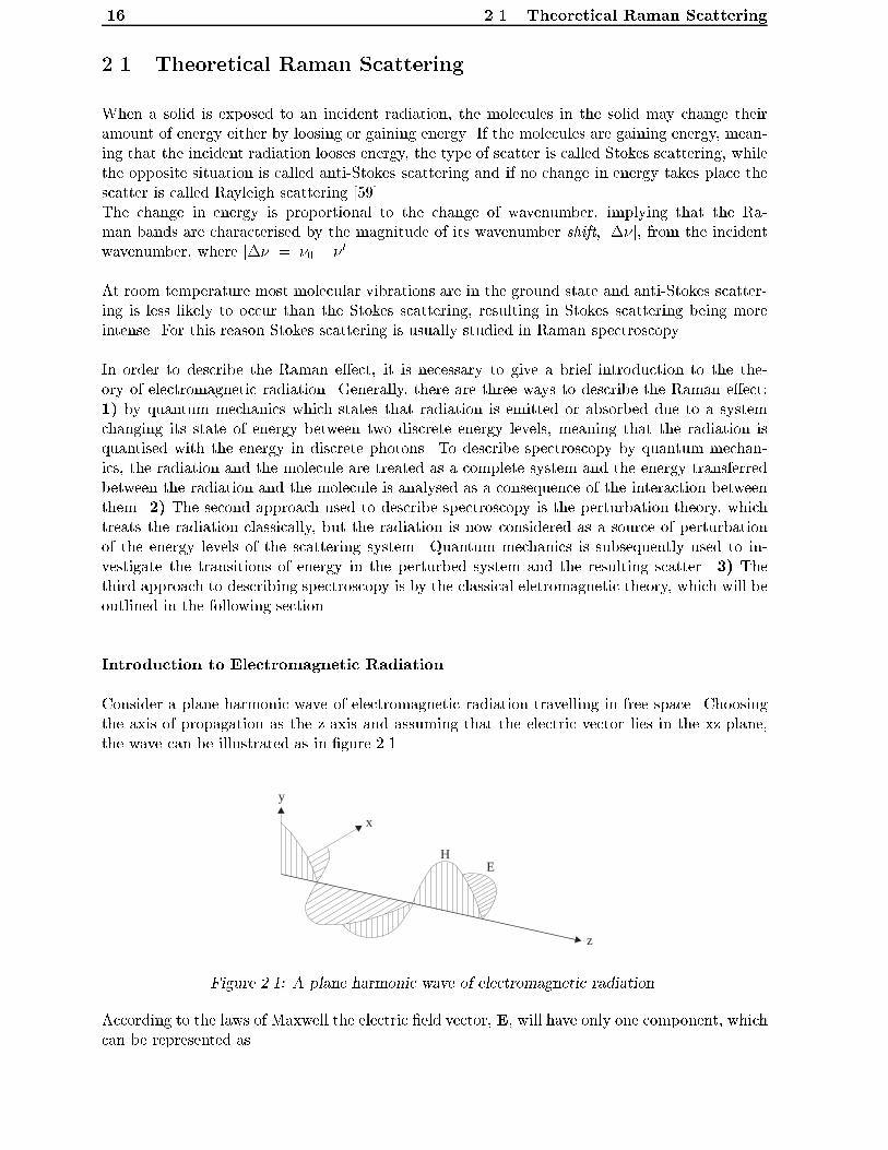
Consider a plane harmonic wave of electromagnetic radiation travelling in free space. Choosingthe axis of propagation as the z-axis and assuming that the electric vector lies in the xz-plane,the wave can be illustrated as in �gure 2.1.
HE
z
x
y
Figure 2.1: A plane harmonic wave of electromagnetic radiation.
According to the laws of Maxwell the electric �eld vector, E, will have only one component, whichcan be represented as

Chapter 2. Raman Spectroscopy 17
Ex = Ex0 cos
�!
�t� z
c
�+ �x
�(2.1)
where Ex0 is the amplitude of Ex, ! is the angular frequency, t is time, z is the position alongthe z-axis, c is the velocity of propagation and �x is the phase angle.The other component of electromagnetic radiation is the magnetic �eld vector, H, which is per-pendicular to the electric �eld vector. In the plane situation the magnetic �eld vector has onlyone component which can be expressed as
Hy = Hy0 cos
�!
�t� z
c
�+ �y
�(2.2)
where Hy0 is the amplitude of Hy and �y = �x in the situation shown in �gure 2.1.
The Dipole
The dipole is the source of Rayleigh and Raman scattering and as such it is a very impor-tant quantity in the theoretical description of Raman scatter. The major contributor to Ramanscatter is the electric dipole and for this reason the magnetic dipole will be omitted here.The electric dipole arises when two charges, equal in magnitude and of opposite sign, are dis-placed relatively to each other. Thus the dipole moment, Pi which is a vector, is de�ned by
Pi = qsi (2.3)
where si is the vector pointing from the charge �q towards the charge q.
Imagine a molecule with a given distribution of electrons. If the molecule is in its equilibriumcon�guration it vibrates with a certain frequency. When the molecule is exposed to an externalelectric �eld, the distribution of electrons is changed and dipoles are created. These dipoles canoscillate and cause radiation. The frequency with which the dipoles oscillate, are determined bythe frequency of the electric �eld and the frequency of the molecular vibration. It readily followsthat the harmonic vibration of a dipole vibrating with the angular frequency !, can be expressedas
Pi = Pi0 cos!t (2.4)
where Pi0 is the amplitude vector of the vibrating dipole.
The Polarisability tensor
Light scattering phenomena can be described in a classical manner in terms of the electromag-netic radiation caused by the dipoles induced in the scattering system by electric and magnetic�elds of the incident radiation.
The induced electric dipole, Pi, can be described in terms of a power series of the electric �eld,Ek as
Pi = P(1)i + P
(2)i + P
(3)i + : : : (2.5)

18 2.1. Theoretical Raman Scattering
where P(j)i are given by
P(1)i = �ikEk
P(2)i =
1
2�iklEkEl (2.6)
P(3)i =
1
6 iklmEkElEm
where �ik, �ikl and iklm are tensors. This stems from the fact that, in general, the direction ofthe dipole is not coincident with that of the electric �eld causing it.More precisely the tensor �ik is a second order tensor and is termed the polarisability tensor.Its components has units of C� m2/V. The tensor �ikl is a third order tensor and is called thehyperpolarisability tensor and its components has the units of C� m3/V2. Finally the tensor iklmis a fourth order tensor and is called the second hyperpolarisability tensor, and its componentshas units of C� m4/V3.These tensors can be interpreted as a measure of the ease with which the electrons can be dis-placed and thereby create a dipole under the action of an electric �eld.
Typically the magnitudes of the components of �ij , �ikl and iklm are 10�40 C� m2/V, 10�50
C� m3/V2 and 10�61 C� m4/V3, respectively [59]. For this reason the tensors �ikl and iklm areusually neglected when considering Raman scatter.This leads to the following expression relating the electric �eld and the dipole
Pi = �ijEj (2.7)
where i; j = 1; 2; 3, corresponding to the three directions in a cartesian coordinate system.�ij is a symmetric tensor, �ij = �ji, meaning that there are only six di�erent components andobviously �ij transforms in a manner analogous to the stress and strain tensors
�l0k0 = bl0ibk0j�ij (2.8)
where bl0i and bk0j are direction cosines between the axis l0i and k0j respectively.The polarisability tensor also has invariants, the �rst is the mean polarisability de�ned as
a =1
3�kk (2.9)
and the second invariant is de�ned as
2 =1
2
n(�11 � �22)
2 + (�22 � �33)2 + (�33 � �11)
2 + 6(�212 + �223 + �231)o
(2.10)
As in three dimensional plasticity, the Mises yield surface is a cylinder, the second invariant ofthe polarisability tensor can also be given a graphical representation, which is an ellipsoid. Whenthe cartesian coordinate axes are coincident with the ellipsoidal axes, these axes correspond tothe principal axes, which is analogous to the principal stress and strain axes in the theory ofelasticity.
Chapter 2. Raman Spectroscopy 19
Classical Raman and Rayleigh Scattering
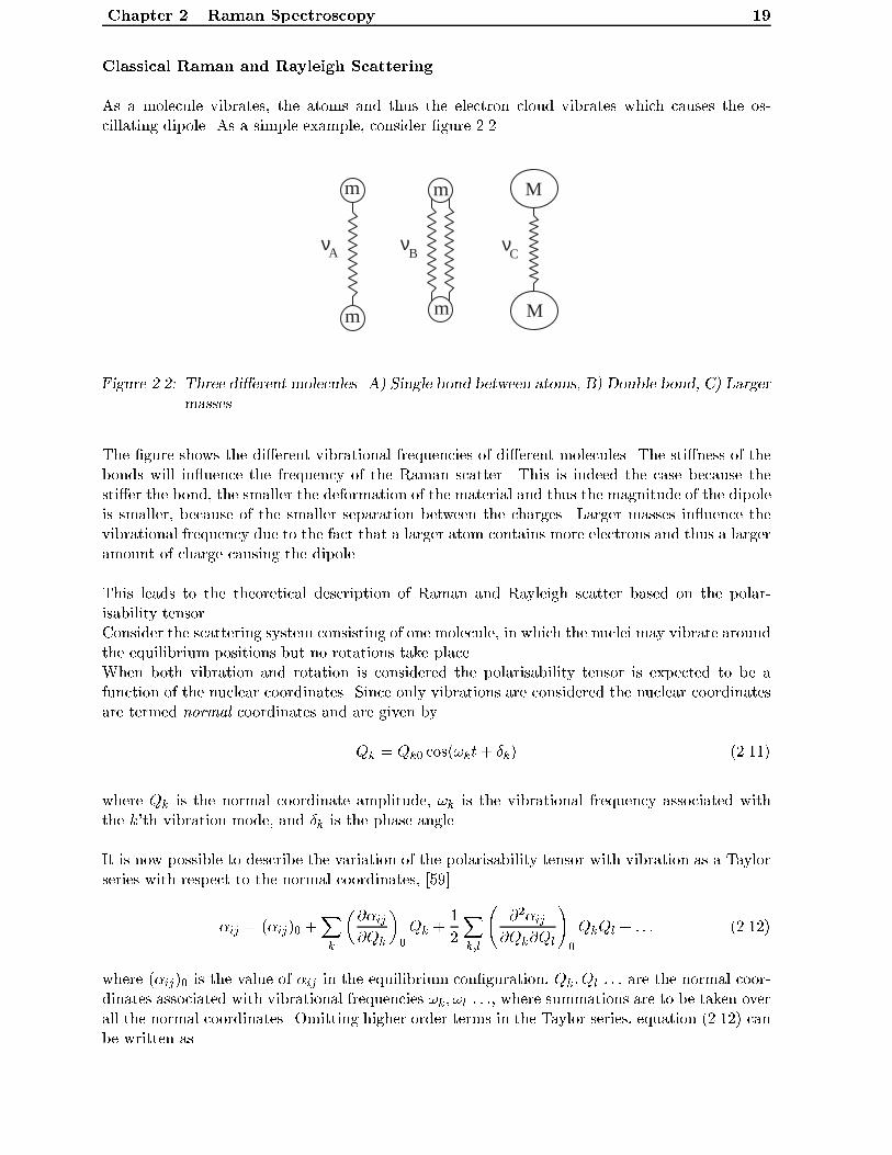
As a molecule vibrates, the atoms and thus the electron cloud vibrates which causes the os-cillating dipole. As a simple example, consider �gure 2.2.
mm
m m
M
M
ν ν νA B C
Figure 2.2: Three di�erent molecules. A) Single bond between atoms, B) Double bond, C) Larger
masses.
The �gure shows the di�erent vibrational frequencies of di�erent molecules. The sti�ness of thebonds will in uence the frequency of the Raman scatter. This is indeed the case because thesti�er the bond, the smaller the deformation of the material and thus the magnitude of the dipoleis smaller, because of the smaller separation between the charges. Larger masses in uence thevibrational frequency due to the fact that a larger atom contains more electrons and thus a largeramount of charge causing the dipole.
This leads to the theoretical description of Raman and Rayleigh scatter based on the polar-isability tensor.Consider the scattering system consisting of one molecule, in which the nuclei may vibrate aroundthe equilibrium positions but no rotations take place.When both vibration and rotation is considered the polarisability tensor is expected to be afunction of the nuclear coordinates. Since only vibrations are considered the nuclear coordinatesare termed normal coordinates and are given by
Qk = Qk0 cos(!kt+ �k) (2.11)
where Qk is the normal coordinate amplitude, !k is the vibrational frequency associated withthe k'th vibration mode, and �k is the phase angle.
It is now possible to describe the variation of the polarisability tensor with vibration as a Taylorseries with respect to the normal coordinates, [59]
�ij = (�ij)0 +Xk
�@�ij@Qk
�0
Qk +1
2
Xk;l
@2�ij@Qk@Ql
!0
QkQl + : : : (2.12)
where (�ij)0 is the value of �ij in the equilibrium con�guration, Qk; Ql : : : are the normal coor-dinates associated with vibrational frequencies !k; !l : : :, where summations are to be taken overall the normal coordinates. Omitting higher order terms in the Taylor series, equation (2.12) canbe written as

20 2.1. Theoretical Raman Scattering
(�ij)k = (�ij)0 + (�0ij)kQk (2.13)
where (�0ij)k =�@�ij@Qk
�0.
When the molecule is exposed to an electromagnetic radiation of the form
Ei = Ei0 cos!0t (2.14)
the induced dipole can be expressed as
P(1)i = (�ij)kEj (2.15)
Inserting equations (2.14), (2.13) and (2.11) into equation (2.15), leads to
P(1)i = (�ij)0Ei0 cos!0t+ (�0ij)kEi0Qk0 cos!0t cos(!k + �k) (2.16)
(�0ij)k is also known as the \Raman tensor" and is essential when considering polarised Ramanspectroscopy.After using some mathematical manipulations equation (2.16) can be expressed as, [59]
P(1)i = P
(1)i (!0) + P
(1)i (!0 � !k) + P
(1)i (!0 + !k) (2.17)
The �rst term in equation (2.17) give rise to scattering with frequency !0, and so accounts forRayleigh scattering. The second term give rise to scattering with frequency !0 � !k and thusaccounts for Stokes-Raman scattering. The last term give rise to scattering with vibrational fre-quency !0+!k and thus accounts for anti-Stokes Raman scattering. The three kinds of scatteringoccurs when:
Rayleigh scattering: arises from the dipole oscillating at vibrational frequency !0, when themolecule is exposed to the electric �eld which itself oscillates with frequency !0.
Raman scattering: arises from the dipoles oscillating with frequency !0 � !k. This occurs whenthe dipoles are oscillating with frequency !0 and these are a�ected by the molecule oscillatingwith frequency !k.
Thus one of the main conditions for a material to be Raman active is that the partial derivativeof the polarisability tensor, with respect to the normal coordinates, must have non-zero compo-nents. This implies that there must be a change in the polarisability with the vibration of themolecule. As a consequence of this fact polarised Raman spectroscopy can be used to conductmeasurements in a polymer in a way similar to classical photoelasticity.
As mentioned before di�erent molecules possesses di�erent Raman frequencies. Some of thesefrequencies will shift under an application of load. This is quite easy to show. Consider �gure2.2. The following system of equations can be established to determine the eigen frequency ofthe system
det
"(�m0!2 + k0) �k0
�k0 (m0!2 + k0)
#= 0 (2.18)

Chapter 2. Raman Spectroscopy 21
where m0 and k0 are the equivalent mass and sti�ness of the system, respectively. In general thisequation can be written in a compact form as
det(B� !2I) = 0 (2.19)
which constitutes a matrix equation in which I is the identity matrix and B incorporates boththe equivalent mass and sti�ness. ! is the eigen frequency of the system and det denotes thedeterminant of the matrix. If a force is applied to the system in �gure 2.2 the resulting displace-ment causes a larger force between the atoms. This additional force is analoguous to a change,�B, in the matrix B. Now the equation to determine the frequency reads [96]
det�(B+�B)� 2I
�= 0 (2.20)
where the frequency shift is obtained as �� = � !. The derivations above show that appli-cation of a load causes a change of frequency. This phenomenon provides the basis for strainmeasurements in e.g. the reinforcing �bres in �bre composites. All that is required for the strainmeasurements is a calibration curve relating frequency shift and applied strain as will be shownlater.
2.2 Experimental Setup
In this section parts of the experimental setup are described. First a description of the Ramanspectrometer is given, followed by a description of the straining rig which has been constructedin order to apply the various load histories.
The spectrometer
Attached to the spectrometer is a modi�ed Olympus microscope which serves to locate thedesired area in the sample and to enhance resolution. The laser beam is directed on to thesample through the optics of the spectrometer and then through the microscope. Using thisexperimental setup it is possible to focus the laser spot to a diameter of about 1-2 �m and recordRaman spectra from this area. The scattered radiation from the sample goes back through themicroscope and into the spectrometer as shown in �gure 2.3. An additional description of someof the parts follows and a photograph of the spectrometer is shown in �gure 2.4.
a) The laser alignment mirror is used to make sure that the laser is perfectly aligned.
b) The objective lens and the pinhole serves to provide a well de�ned laser spot.
f) The beam splitter allows only Raman scattered light to pass through. This means that theCCD camera will only be exposed to Raman scattered light and not to Rayleigh scattered light.
g) The polariser is fundamental for determining vibration modes and symmetry of vibrations.This is due to the fact that the intensity of the actual vibration changes when changing thepolarisation of the excitation radiation.

22 2.2. Experimental Setup
abc
d
e
fg h
k
i
j
Laser
Excitation radiationto sample
Scattered radiationfrom sample
x
y
z
Figure 2.3: The major parts of the spectrometer. a) Laser alignment mirror. b) Objective lens
and 10 �m pinhole. c) Spot focus adjustment lens. d) Adjustable mirror. e) Fixed
mirror. f) Beam splitter. g) Polariser. h) Spatial �lter. i) Grating. j) Isosceles
triangular mirror. k) CCD chip.
Figure 2.4: The spectrometer.
h) The spatial �lter allows the examination of samples where the region or particle of inter-est cannot be physically isolated from the remainder of the sample. Spectral interferences fromthe surrounding area can be minimised or eliminated by isolating the region of interest with aspatial �lter.
i) The grating consists of a series of grooves ruled on a hard glassy or metallic material. Thesegrooves are extremely closely spaced, spacings of 1 �m are not unusual, [41]. The grating dispersesthe scattered light and then passes it through a narrow slit so that the light passing through tothe detector at any time has a very narrow band width and may be considered as essentiallymonochromatic. The spectrum is produced by rotating the grating so that a continuously chang-ing wavelength is presented to the detector.

Chapter 2. Raman Spectroscopy 23
j) The di�erent wavelenghts from the grating are exposed to di�erent areas of the CCD chipby the triangular mirror.
k) The CCD chip is the device which detects the scattered radiation and produces the spectrum.It is a two-dimensional array of silicon photosensors, each photosensor usually being referred toas a pixel. When radiation falls on a pixel, photoelectrons are produced in numbers proportionalto the intensity of the radiation. A typical CCD contains about 2000 columns and 800 rows ofpixels, where the area of each pixel is 15 �m � 15 �m.
The spectrometer is operated by appropriate software installed on a PC. The PC serves both asa data collector and as controller of �lters and motors in the spectrometer. Furthermore, thePC controls the fully automatic motorised xyz-stage, the heating device and the straining rig.Additional software provides the tools for data analysis.
The Straining Rig
Figure 2.5: The straining rig.
The straining rig was purpose build to �t under the Raman microscope and is shown in �gure2.5. The straining rig is constructed as a conventional tensile testing machine with two columnscarrying the load. Two plates at each end of the rig serve as base for the load transducer andthe gearbox, respectively. The gear box is belt driven in order to minimise noise and vibrationstransmitted to the microscope. The specimen is held by two guides in which spherical bearingsare mounted to ensure that no bending e�ects are applied to the specimen. Clamps with a shapeexactly like the specimens ends are mounted in these bearings. This ensures that no stress con-centrations are introduced into the specimens. One of the guides is connected to the gear boxvia a spindle and can slide along the columns in slide bearings and thereby provides the lineardisplacement that creates the tension in the specimen. A stepper motor with a resolution of 1.8�
per step is connected to the gear box. This resolution gives a linear displacement of 4 �m per

24 2.3. Applications of MRS
step. The load transducer is connected to a strain gauge ampli�er and a data acquisition module.The signal from from the strain gauge ampli�er is used to control the stepper motor, thus thestraining rig is force controlled, allowing application of di�erent loading histories, such as steploading, creep loading or conventional tensile testing.
2.3 Applications of MRS
This section includes a literature survey of papers covering a broad range of MRS applicationsin order to pinpoint the possibilities and limitations of the technique and serves as a basis forspecifying the experimental programme. Additionally, the section describes some of the practicaldetails concerning strain measurements with MRS.
Even though the Raman e�ect has been known for quite some time it was not used for strainmeasurements until the late 1970's. The idea of using Raman spectroscopy for strain measure-ments in crystalline materials initiated when Robert Young and David Batchelder was discussingtwinning of polydiacetylene crystals, during a co�ee break at Queen Mary and West�eld Collegein London, [135]. After the initiation of the concept of strain measurement with MRS, Batchelderand Bloor [4], showed that polydiacetylene crystals posseses four strain dependent Raman fre-quencies, situated at 2080 cm�1, 1480 cm�1, 1200 cm�1 and 950 cm�1. They also showed thatthe strain sensitivity of these four peaks are: -20 cm�1/%, -9.9 cm�1/%, -0.4 cm�1/% and -7.6cm�1/%, respectively.
Later on Galiotis et al. [31] found that aramid �bres possess a strain sensitive Raman bandas well, situated at 1610 cm�1. Later on these �ndings were refuted by other workers, but thedisagreement was �nally resolved by Young et al. [132] who found that high powered lasers (>1W) caused premature failure of aramid �bres. Young et al. also found the strain sensitivity tobe -4.1 cm�1/%.
The �rst researchers to report strain induced frequency shifts in carbon �bres were Robinsonet al., [92]. They showed that carbon �bres usually possess two major �rst order Raman bandsat 1360 cm�1 and 1580 cm�1 which shift to a lower wavenumber under the application of a tensileload. The strain sensivity of these bands are approximately -7 cm�1/% and -9 cm�1/%.
After these pioneering investigations it was obvious that the Raman technique is a powerfultool for in-situ non destructive investigations of various micromechanical phenomena in compos-ite materials.
Huang and Young [43] investigated the interfacial behaviour of high temperature cured carbon�bre/epoxy resin model composites. They evaluated the interfacial shear strength by Ramanspectroscopic analysis of the traditional fragmentation test. They found that the interfacialshear strength was higher in the hot-cured specimens than in the equivalent cold-cured speci-mens. It was found that the stress transfer from the �bre to the matrix was well modelled by theCox shear-lag theory at low levels of applied stress. At higher levels of applied stress the stresstransfer mechanism is a combination of elastic shear stress in the bonded region and frictionalshear stress in the debonded region. Also in the debonded region a higher shear stress was foundin the hot-cured specimens, due to the e�ect of thermal expansion mismatch.
Paipetis and Galiotis [79] investigated the e�ect of �bre sizing on the stress transfer e�encyin carbon/epoxy model composites. They found that the interfacial shear strength was higher

Chapter 2. Raman Spectroscopy 25
in the sized system than in the unsized. The interfacial shear strength determined from theKelly-Tyson model was found to be 42 MPa which compares well to the shear yield strength ofthe resin.The residual stress in the �bre was measured in 20 identical specimens and found to be indepen-dent of the sizing and was of the order of 2000 MPa. However, upon loading mode II debondingwas observed in the unsized system whereas the sized system sustained a higher shear stressleading to a mixed mode cracking.
Another application of Raman spectroscopy is monitoring interaction e�ects between �bres in2-dimensional model composites. Such investigations have been undertaken by Schadler et al.[95] and Chohan and Galiotis [15] on carbon/epoxy specimens. Wagner et al. [117] investigatedinteraction e�ects in model composites with Kevlar �bres. Grubb et al. [35] investigated the �berinteractions in hybrid model composites by embeddeding one carbon �bre along with two Kevlar�bres on each side in an epoxy resin. Generally, the interaction distance is found to be � 5 timesthe carbon �bre diameter. The strain concentration factor is approximately 1.5 which is lessthan predicted by the applied shear lag analysis. In the Kevlar specimen the strain concentrationfactor is around 1.1 which is due to the fact that Kevlar �bres are not as brittle as carbon �bresbut instead display a region of damage which carries no load. Furthermore, these investigationsshowed that axial stresses in the matrix is not negligible as assumed by the shear-lag theories.
Strain measurements in polymeric �bres have been undertaken by Young and Yeh [133], whoinvestigated the mechanical straining of PET �bres and found that the Raman frequency shiftwas stress related.Grubb and Li [36] investigated the molecular stress distribution and creep of high-modulus PE�bres and found that the molecular structure undergoes complex changes during creep.Hu et al. [45] used the strain sensitivity of diacetylene to measure the strain in a diacety-lene/urethane copolymer at various angles of polarization and found that the results were inagreement with the theory of elasticity.Rodriguez-Cabello et al. [93] investigated the chain deformation of uniaxially stretched bulk PEand found that the transfer of the load on the polymer backbone was not e�ective until thesample showed a high degree of orientation in the stretching direction.Mermet et al. [67] investigated the plastic deformation of PC and found that the cohesive regionsin the polymer was a�ected di�erently and that the shape of the spectra were di�erent whenthe temperature was lower and higher than the glass transition temperature, respectively. Thisis due to the larger mobility of the molecular chains at temperatures above the glass transitiontemperature.
In all the afore mentioned studies the Raman frequency shifts were used to determine the strainsand molecular stress distribution. This is possible because of the highly orientated polymerchains. The stretching of the polymer chains causes the polymer backbone to be stretched, whichagain causes the frequency shifts.However, such opto-mechanical behaviour is much more di�cult in isotropic polymers becausethey show no stress or strain induced frequency shifts until a very large strain is applied. The rea-son is, that initially the polymer chains are more or less randomly oriented in the bulk polymer,but when the load level is increased a larger degree of orientation is observed for the polymerchains and the same tendencies as for the �bre can be observed. As seen in [67] both a frequencyshift and a broadening of the Raman band occurs for deformed PC specimens. Unfortunatelythe deformed specimens are strained to above 90 %, which is not appropriate for the present study.
The former investigations are based on the strain dependent frequency shifts of the �bres. How-ever, Raman spectroscopy can also be used for other investigations than strain measurements.

26 2.3. Applications of MRS
By comparing the shape and intensities of the various bands in the Raman spectra it is possibleto determine the fractions of crystalline and amorphous phases in a semi crystalline polymer.This technique has been used by Keresztury and F�oldes [50] in an analysis of polyethylene, andby Nielsen and Pyrz [74] in an investigation of the crystalline phase in uence on thermal strainsin carbon �bre/polypropylene matrix composites during cool down.
To measure the strains in isotropic polymers another feature of the Raman spectra needs tobe taken in to consideration. Namely the dependence of polarization on the incident and scat-tered light on the frequency shift. The reason is that for polymers of low orientation, observationswith di�erent polarization combinations are selectively sensitive to chains oriented in di�erentdirections and these chains are in di�erent states of stress/strain. This leads to the possibilityof obtaining information about the distribution of stress/strain in chains at di�erent orientationto the loading direction, [75]. Applying a known stress state to the polymer and recording thespectra yields the "reference" spectra. These spectra are compared to the spectra obtained fromthe vicinity of an embedded �bre and the strains around an embedded �bre can be determined.However, at present, this technique seems only to be applicable to polymers which are also suitedfor classical photo elasticity, i.e. amorphous birefringent polymers.
In spite of the large number of papers concerning strain measurements on composites the Ramantechnique has not been used on composites during creep. To the authors knowledge only a fewinvestigations concerning viscoelasticity in composites have been conducted.
Sengonul and Wilding [108] used the Raman technique to monitor viscoelasticity in ultra highmodulus polyethylene, (UHMPE), �bres. They used the Raman spectroscopy to interpret thetime dependent behaviour of UHMPE and subsequently model these e�ects by simple spring/dash-pot models. These models are used to predict the Raman frequency shifts on strain. The pa-rameters in the models are determined by best �t to experimental data. The creep behaviour isquite well modelled, but the relaxation modelling fails to reproduce the observed phenomena.
A theoretical investigation of the stress induced shifts for isotropic and uniaxially orientatedPET have been carried out by Bower et al. [9] and an experimental investigation by Lewis et al.[54]. They found that neither a strain or stress governed model �ts the experimental data well.Most important is the conclusion that the observed shifts depend only on the applied stress anddo not change as the sample creeps.
Based on the previous literature study it was decided that the experimental approach shouldbe based on �bre strain measurements using MRS. Additionally, traditional optical microscopyand SEM will be used when appropriate.
In all the Raman measurements the incident laser light was polarised in the yz-plane, see �gure2.3 and 2.4, and the loading direction of the straining rig was parallel to the x-direction.Equipment for changing the polarisation direction of the incident laser light was only purchasedrecently and has not been used in the present work.
Determination of Strain Sensitivity of Carbon Fibres
To measure the strains in a carbon �bre composite it is necessary to know which of the Ra-man bands are strain sensitive. For HM PAN based carbon �bre there are generally three mainRaman bands. These are �1 � 1360 cm�1, �2 � 1580 cm�1 and �3 � 2700 cm�1. The 1360cm�1 frequency is an A1g vibration mode due to crystal boundary regions in the graphite and

Chapter 2. Raman Spectroscopy 27
has been attributed to a crystalline size e�ect. The second frequency is attributed to the in-planestretching of the C-C bonds in the �bre and is due to an E2g vibrational mode in the graphitecrystals. The last frequency at 2700 cm�1 is a second order band [92]. The three frequencies inthe spectrum of the used carbon �bres are shown in �gure 2.6.
150
250
350
450
550
1000 2000 3000
Inte
nsity
[a.u
.]
Raman frequency [cm ]-1
Figure 2.6: The three strain sensitive Raman peaks in a HM carbon �bre.
In this analysis high modulus carbon �bres of the type Tenax-J from Toho Rayon are used. Thefrequency used for the strain measurements is the 2660 cm�1 peak, due to its high strain sensivity.
Figure 2.7: The bending rig.
To determine the peak position dependence upon strain a simple bending test is performed. Asmall straining rig have been constructed, consisting of a clamp and a micrometer dial gauge. Acarbon �bre is glued on top of a polymeric beam and inserted into the clamp in the bending rig.The dial gauge is used to apply a known deformation to the cantilever beam, and from the beamtheory the strain in the �bre can be determined from the expression
" =3h�
2L2
�1� x
L
�(2.21)
where h is the height of the beam, � is the de ection, x is the distance from the clamped end tothe point of measurement and L is the length of the beam. The bending rig is shown in �gure 2.7.
The tensile strain sensitivity of the �bres was found to be -23 cm�1/%, which is consistent

28 2.4. Summary
with values reported by Young [134] and the compressive strain sensitivity has been found byNielsen and Pyrz [74] to be -20 cm�1/%. The experimental values along with the �tted straightline are shown in �gure 2.8. From measurements on unloaded carbon �bres in free air, the fre-quency at which the �bres are unstrained has been found to be 2661 cm�1.
Galiotis and Batchelder [30] found that the 2660 cm�1 Raman band is nonlinear for strainslarger than 0.6 %. However, strains of this magnitude will not appear in the present work andtherefore this nonlinearity is disregarded. In the present study only one �bre type have been usedbut in the discussion of strain sensitivity it is important to mention that the strain sensitivityalso depends on �bre moduli. Huang and Young [44] found that the strain sensitivity of bothPAN and pitch based carbon �bres increased linearly with increasing �bre moduli. Furthermore,they found that the stress dependence of Raman shift was independent of �bre modulus.
2660
2650
2640
2630
0 0.4 0.8 1.2
Ram
an fr
eque
ncy
[cm
]
-1
Strain [%]
Figure 2.8: The strain sensitivity of the carbon �bres, measured on di�erent �bres.
2.4 Summary
The basic theory of Raman scattering has been outlined and it has been shown - by simplemechanical considerations - that application of a load will shift some of the Raman bands incrystalline materials. The relationship between applied strain and wavenumber shift for the used�bres have been found to be -23 cm�1=% which is consistent with values found in the litterature.Based on a literature study the experimental programme includes �bre strain measurements usingMRS together with SEM and optical microscopy when appropriate.

Chapter
3
Viscoelasticity
This chapter outlines the viscoelastic constitutive model applied to the polypropylenematrix considered in this thesis.
The chapter is divided into three major parts. One discusses some of the theoretical approachesused to describe viscoelastic constitutive behaviour. The major e�ort is placed on the Schaperymodel, because this model will be used in the theoretical modelling. Next, the parameters in theSchapery model are determined from creep and relaxation data and �nally the one dimensionalSchapery model is extended to three dimensions.
Polymeric materials are characterised by the long chain like nature of their molecules. Mostpolymers in this area of interest have molecules based on a carbon backbone with each carbonatom being linked to the two adjacent carbon atoms by covalent bonds.The chains in the molecular structure of a polymer may be linear in the sense that they form longthreads, they may be branched or they may be crosslinked in which case the chains are linkedtogether at various points along their length. In the latter case the molecular chains may form agiant molecular network and constitutes a thermosetting polymer.Thermoplastic polymers can appear as amorphous and semi crystalline. The semi crystallinepolymers also form crosslinks, although these are usually based on secondary bonds such as hy-drogen bonds and Van der Waal bonds, whereas the crosslinks in thermosetting polymers arecovalent.The deformation mechanisms in a thermoplastic polymer are mainly due to extension in themolecular chains and relative motion between adjacent chains. This relative motion is prohibitedin the thermosetting polymers due to the strong crosslinks between the chains.Upon heating, the secondary bonds in thermoplastic polymers will be broken, causing a largerelative motion between the chains and a decrease in sti�ness of the polymer, which can be ofseveral orders of magnitude. These physical and molecular changes in the polymer are the majorcontributors to the viscoelastic behaviour of thermoplastic polymers.
A study of the viscoelastic properties of composite materials is of primarily interest becauseof the considerable number of composites that have a polymeric matrix. This is the case for most�bre composites where the most common polymer matrices are epoxy for unidirectional �brecomposites, polyester for chopped �bre composites and a wide range of thermoplastic polymersfor injection moulded composites. Because of the time dependent properties of the polymer thecomposite will also exhibit time dependence and these e�ects are magni�ed at elevated temper-atures.
29

30 3.1. Viscoelastic Constitutive Models
In the following some viscoelastic models will be presented and �nally the basis of the Schaperymodel will be outlined.
3.1 Viscoelastic Constitutive Models
The most general description of a viscoelastic material is to state the relation between stress andstrain as
"(t) = Jijkl [�(�)]t0�(t) = Gijkl ["(�)]t0 (3.1)
where Jijkl is the fourth order anisotropic creep tensor, (the creep compliance) and Gijkl is thefourth order anisotropic relaxation tensor, (the relaxation modulus).In order to reproduce the observed material deformation behaviour, the viscoelastic constitutivemodel must be able to reproduce history dependence in the sense of fading memory, since thisfeature is possessed by most polymeric and composite materials. Indeed, some composite mate-rials even possess permanent memory, manifesting itself as hysteresis under repeated loading oras plasticity under static loading.The fading memory characteristic is that the material responds less to events in the distant pastin its history than to recent ones. In the linear situation this means that the rate of changeof the relaxation and creep tensors are a�ected less as time increases, thus the magnitude ofthese tensors are continuously decreasing with increasing time. In the nonlinear situation it issomewhat more complicated and demands the existence of the Fr�echet di�erential, [17].
The following discussion of constitutive models will be concerned with some of the integral basedconstitutive models.
The most general formulation of the relations above is that due to Green and Rivlin [34]. Thisapproach is basically a polynomial expansion of the stress history, expressing the strain as linearfunctionals. In the one dimensional case this constitutive relation can be stated as
"(t) =
Z t
0�1(t� �1) _�(�1)d�1 +
Z t
0
Z t
0�2(t� �1; t� �2) _�(�1) _�(�2)d�1d�2
+
Z t
0
Z t
0
Z t
0�3(t� �1; t� �2; t� �3) _�(�1) _�(�2) _�(�3)d�1d�2d�3 + : : : (3.2)
where �i are creep compliances and �i are the times at which the stresses are applied.It is seen that the �rst term is the linear Boltzmann superposition integral. Furthermore, it isimportant to notice that this model is not capable of modelling the response of an ageing materialbecause the kernels are functions of (t� �i) only and not of (t; �i), i.e. the kernels are invariantwith respect to time translation. The second and higher order terms account for magnitude andinteraction nonlinearity between di�erent loading components. The kernels can be determinedby application of stepwise loading and the number of kernels corresponds to the number of steps.
Even though this model is very general, it is not suited for application. If the material ofinterest exhibits strong nonlinearities several terms are needed. To determine �i in equation(3.2) 78 experiments are needed, whereas a third order approximation of the three dimensional

Chapter 3. Viscoelasticity 31
case involves 12 kernels and according to Lockett, [58] this demands 463 experiments. This factmakes it very tedious to utilise the model.
As an alternative approach the kernels can be nonlinearised by introducing stresses or stressrates into the kernels.This approach was proposed by Pipkin and Rogers [86] and their one dimensional constitutivemodel may be stated as
"(t) =
Z t
0�1[t� �; �(�)] _�(�)d� +
Z t
0
Z t
0�2[t� �1; �(�1); t� �2; �(�2)] _�(�1) _�(�2)d�1d�2
+
Z t
0
Z t
0
Z t
0�3[t� �1; �(�1); t� �2; �(�2); t� �3; �(�3)] _�(�1) _�(�2) _�(�3)d�1d�2d�3 (3.3)
The motivation for proposing this model was that the �rst integral should model single steptests exactly, the second term should extend the exact representation to two step tests etc. Animportant aspect pointed out by Lockett [58], is that this equation cannot be used as a basisfor systematic determination of material properties unless the material happens to be completelyde�nable in one step tests. This stems from the fact that the second term involves a function offour variables and a systematic experimental programme would be prohibitive.
The third model considered is a single integral representation, known as the Rabotnov model.The Rabotnov model is based upon the assumption that the kernels in the expression
"(t) =
Z t
0J1(t� �1)d�(�1) +
Z t
0
Z t
0J2(t� �1; t� �2)d�(�1)d�(�2) + : : : (3.4)
are separable and expressable as
Ji(t� �1; t� �2; : : : ; t� �i) = ai
iYn=1
J0(t� �n) (3.5)
where ai is a constant and J0 is the same for all time arguments (t��n). Choosing an appropriateintegral operator K�, equation (3.4) can be written as
�(") = � +K�� (3.6)
where K�� is given by
K�� =
Z t
0K(t� �)�(�)d� (3.7)
which gives the creep strain for an applied stress �0 as
�(") = �0
�1 +
Z t
0K(t� �)d�
�(3.8)
where �(") incorporates both the instantaneous stress-strain curve and the deviation from theinstantaneous curve due to time e�ects. However, equation (3.8) is of no use if the kernel is

32 3.2. The Schapery Model
unknown. Rabotnov proposed the following expression for the kernel K(t), [87]
K(t) =e��t
t
1Xn=1
[A�(�)]nt�n
�(�n)(3.9)
where A, � and � are constants and � is the Euler function. Having determined these constantsthe response to an applied load of a material is readily obtainable from equation (3.6).According to Pyrz [87], a remarkable feature of equation (3.6) is that it describes the creep de-formation, the recovery deformation, the relaxation and the stress rate dependence correctly fora variety of isotropic materials and composite materials.
Another single integral model is the endochronic model suggested by Valanis, but since thisis a special case of the Schapery model it will not be considered further.
As stated earlier, the constitutive description of the matrix material will be based upon thethermodynamic model, proposed by Schapery. The reason for using the Schapery model is thatthis model has shown to give very accurate results compared to experiments.This theory has a number of desirable features, [58]. The ability to describe strong nonlinearityof some materials and the nonlinearity with respect to strain is contained in the form of functionsrather than polynomials which are not the most convenient form. The polynomial formulationcan lead to wrong conclusions such as predictions of compressive behaviour from tensile data.Furthermore, because of the dependence of material functions of only one variable, the experi-mental programme is not prohibitive.
The Schapery model appears to describe the deformation behaviour very well, for both stressand strain inputs, [87]. The ability of the model to describe viscoelastic behaviour have beenshown by Schapery [101], [102] and Lou and Schapery [60], by applying the model to a varietyof materials.
Another advantage, compared to the multiple integral representations, is that it is quite straightforward to use the Schapery model to describe experimental data, whereas the multiple integralrepresentations are virtually impossible to verify in practice.
The Shapery model is based upon the thermodynamics of irreversible processes, and uses theconcept of internal state variables. The theory is developed in a series of publications, [99] - [101]and is basically an extension of the work of Biot [7].
3.2 The Schapery Model
The state of a material is de�ned by the generalized state variables �, which are divided into twogroups, of observed variables �m (m = 1; 2; : : : k) and hidden variables �r (r = k+1; k+2; : : : n).To each state variable the conjugate forces are denoted by �m and �r.
The hidden variables are not important in this particular case, since they vanish in the �nalequations, but they can be thought of as representing molecular con�gurations in a polymer orlocation of interstitial atoms in a metal. In the thermodynamic formulation the generalized statevariables need not be restricted, but as will be seen later, six of the observed variables are associ-ated with the six independent components of the strain tensor and the corresponding conjugateforces are associated with the six independent components of the stress tensor.

Chapter 3. Viscoelasticity 33
Constitutive equations must be consistent with the basic principles of continuum mechanics.This implies that the constitutive equation obeys the laws of motion, conservation principles andthe Clausius - Duhem inequality, which is a consequence of the second law of thermodynamic.The derivation of the Schapery constitutive equation, for strains expressed in terms of stresses,is based upon a thermodynamic potential, G, known as the Gibbs free energy. For the oppositesituation, stresses in terms of strains, the Helmholtz free energy potential is used.
By assuming that the concept of entropy is extendable into situations when the system is inthe \neighbourhood" of equilibrium, it is possible, through the Gibbs equation, to equate the in-ternal energy changes for reversible and irreversible processes and obtain an explicit expression forthe entropy production. The entropy production is explicitly related to the various irreversibleprocesses in the system through a linear phenomenological relation, (Onsager's principle), be-tween the forces (�i � �Ri ) and the uxes _�i and is expressed as
(�i � �Ri ) =nX
j=1
bij(�m; T ) _�j (3.10)
This principle states that when the ow _�j corresponding to the irreversible process j, is in u-enced by the force (�i � �Ri ), corresponding to the irreversible process i, then the ow _�i is alsoin uenced by the force (�j � �Rj ) through the same in uence coe�cients, bij(�m; T ).
In this description the term �Ri is the reversible part of the conjugate forces. �Ri is related to �ithrough the Gibb's free energy and thus reduces the problem to the solution of two systems ofequations
�m = �%@G(�m; �r)@�m
m = 1; 2 : : : k
%@G(�m; �r)
@�r+ brs(�m) _�s = 0 r; s = k + 1; k + 2 : : : n (3.11)
where % is mass density. Approximating the Gibbs free energy in a Taylor expansion with respectto the internal variables
%G = %G0(�m) + cr(�m)�r +1
2drs(�m)�r�s (3.12)
where G0 acts as a potential for the time independent response, the second term corresponds tothe energy associated with a simultaneous action on the internal variables �r and the last termis de�ned by the interaction energy associated with the simultaneous action on the internal vari-ables �r and �s, [87]. Substituting the Taylor expansion into equation (3.11) gives the following(n� k) di�erential equations
cr(�m) + drs(�m)�s + brs(�m) _�s = 0 (3.13)
Further simpli�cations are introduced by the assumption that all coe�cients brs(�m) and drs(�m)are a�ected equally by the conjugate forces
brs(�m) = aD(�m)brs
drs(�m) = aG(�m)drs

34 3.2. The Schapery Model
where brs and drs are constant, positive de�nite matrices. aD nonlinearises the entropy produc-tion and aG nonlinerises the interaction energy in the Gibbs free energy expansion, (3.12). Thecoe�cients cr(�m) describes the di�usion of the conjugate forces, �m, into the material structurewhere they a�ect the internal varibles. This nonlinear force transfer process introduces a thirdnonlinearising function ��m, and can be described by
cr(�m) = frm��m(�m)
where frm is a constant matrix.By the simpli�cations and assumptions above it is now possible to reduce the n� k di�erentialequations in (3.13) and obtain a set of di�erential equations with constant coe�cients
aG(�m)drs�s + aD(�m)brsd�sdt
= �frm��m(�m) r; s = k + 1; k + 2; : : : n (3.14)
This set of equations can be rewritten by introducing the reduced time, , as
drs�s + brsd�sd
= � 1
aGfrm��m(�m) (3.15)
where d = (aG=aD)dt. Upon substitution of the free energy expansion, equation (3.12), intothe �rst of equations (3.11) the k algebraic equations are obtained as
�m = �%@G0(�m)
@�m� frm
��m(�m)
@�m�r (3.16)
where the third term in the free energy expansion is neglected. The set of decoupled di�erentialequations, (3.14), can be integrated for the internal variables �s and substituted into the equationabove, thus giving the set of observable variables �m in integral form.
For uniaxial loading only one observed variable �1 exists and is equal to ". The virtual workcondition �W = �i��i = ��" gives the generalised force �1 = �, leading to the one dimensionalSchapery equation
"(t) = �%@G0
@�+@��1(�1)
@�1
Z t
0D( � 0)
@(��1=aG)
@�d� (3.17)
or in the well known form
"(t) = g0D0� + g1
Z t
0�D( � 0)
@g2(�(�))
@�d� (3.18)
where
g0 = �%@G0
@�
1
D0�
g1 =@��1@�1
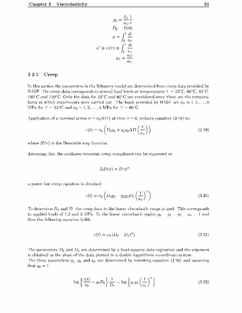
Chapter 3. Viscoelasticity 35
g2 =��1aG
1
�
D0 = D(0)
�Z t
0
dt
a�
0 � (�) �Z �
0
dt
a�
a� =aDaG
3.2.1 Creep
In this section the parameters in the Schapery model are determined from creep data provided byBASF. The creep data corresponds to several load levels at temperatures T = 23�C, 60�C, 80�C,100�C and 120�C. Only the data for 23�C and 60�C are considered since these are the tempera-tures at which experiments were carried out. The loads provided by BASF are �0 = 1; 2; : : : ; 8MPa for T = 23�C and �0 = 1; 2; : : : ; 4 MPa for T = 60�C.
Application of a nominal stress � = �0H(�) at time � = 0, reduces equation (3.18) to:
"(t) = �0
�D0g0 + g1g2�D
�t
a�
��(3.19)
where H(�) is the Heaviside step function.
Assuming that the nonlinear transient creep compliance can be expressed as
�D( ) = D1 n
a power law creep equation is obtained
"(t) = �0
�D0g0 + g1g2D1
�t
a�
�n�(3.20)
To determine D0 and D1 the creep data in the linear viscoelastic range is used. This correspondsto applied loads of 1,2 and 3 MPa. In the linear viscoelastic region g0 = g1 = g2 = a� = 1 andthus the following equation holds
"(t) = �0 (D0 +D1tn) (3.21)
The parameters D0 and D1 are determined by a least squares data regression and the exponentis obtained as the slope of the data plotted in a double logarithmic co-ordinate system.The three parameters g1, g2 and a� are determined by rewriting equation (3.20) and assumingthat g0 = 1
log
�"(t)
�0� g0D0
�1
D1= log
�g1g2
�t
a�
�n�(3.22)

36 3.2. The Schapery Model
and using a least squares data regression gives g1g2an�
.
The assumption that g0 = 1 is supported by Brueller [11], who has investigated the nonlinearlong term behavior of the polymeric materials; poly-methylmethacrylate (PMMA), poly-styrene(PS), poly-oxymethylene (POM) and styrene-acrylonitriles (SAN).The most important consequence of the fact that g0 = 1 is that the instantaneous response -to an applied load - of the polymeric material is always linear, even in the nonlinear range, i.e.yielding is not accounted for.
Due to the lack of recovery data it is not possible to distinguish between the three nonlinearizingparameters g1, g2 and a�. Due to this fact, it is assumed that the product g1g2 is equal to unityand thereby placing all the nonlinearity on a�. This assumption is indirectly validated by thephysical nature of the parameters. The parameters g0, g1 and g2 re ect third and higher orderstress dependence of the Gibb's free energy, whereas a� re ects stress dependence on both theentropy production and free energy. Since the entropy production (Second law of thermodynam-ics) restricts the nature of constitutive models it would be inconsistent to assume that a� equalsunity and instead place the nonlinearity on some of the other parameters.The assumption that g1g2 equals unity is also indirectly supported by experiments by Hiel [39],Xinran [131] and Lou and Schapery [60]. They found that g1 is a slightly decreasing function ofstress, whereas g2 is a slightly increasing function of stress, and thus the product equals unity toa good approximation.It should be noted here that the case of g0 = g1 = g2 = 1 and letting all nonlinearity be due toa� is analogous to what Valanis proposed in his rate independent \plasticity" theory. However,that theory was based upon ideas provided by Schapery in 1969.
The expressions for a� as a function of stress at temperatures 23�C and 60�C are found tobe
a�(�; 23) = 10(�0:14�+0:41)
a�(�; 60) = 10(�0:36 log(�)�0:83) (3.23)
where � is normalised with respect to the stress at which the material is in its linear range, i.e.� = �app=1 MPa.The creep data and the strains calculated by equation (3.20) are shown in �gure 3.1. For T = 23�C the loads are 1,: : :,8 MPa and for T = 60 �C the loads are 1,: : :,4 MPa.
In summary the creep constitutive equation is found to be
"(t) = �0
�g0D0 + g1g2D1
�t
a�
�n�(3.24)
where n is found to be 0.17 and D1 is 733�10�6 MPa�1. D0 is equivalent to 1=E and is a functionof temperature as shown in the table below.
T [�C] D0 �10�6 [MPa�1]
23 667
60 3480

Chapter 3. Viscoelasticity 37
time [hr.]0 5 10 15 20
ε[%
]
0
0.4
0.8
1.2
1.6
2
A
0 5 10 15 20time [hr.]
2.4
2
1.6
1.2
0.8
0.4
ε [%
]
B
Figure 3.1: The creep data and the predicted strains for polypropylene at A) T = 23 �C and B)T = 60 �C.
As seen in the �gure the experimental creep data and the predicted creep curves show very goodagreement.
3.2.2 Recovery
After removal of the applied load an elastic contraction of the material is followed by a timedependent contraction. This contraction is known as recovery. The strains will asymptoticallyapproach zero as time approaches in�nity - provided that no yielding has occurred. The recoverystrains are modelled by using equation (3.18). Applying a stress �a at time t = ta and a stress �b attime t = tb, carrying out the integration and equating �b to zero yields the recovery strain as [102]
"r(t) = g2D1�
�taa�
�n[(1 + a��)
n � (a��)n] (3.25)
where � is equal to (t� ta)=ta and ta corresponds to the time at which the load, �, is removed.
3.2.3 Relaxation
Relaxation is modelled using the expression by Schapery [102]
�(t) = "0
�heEe + h1h2�E
�t
a"
��(3.26)
where a power law is assumed for the nonlinear relaxation modulus, �E, which leads to
�(t) = "0
�heEe + h1h2E1
�t
a"
�m�(3.27)
The relaxation data are for strain levels of "0 = 0:04; 0:08; 0:2; 0:3; 0:4; 0:6; 0:8 and 1 % attemperature T = 23�C and "0 = 0:08; 0:2; 0:3; 0:4; 0:6; 0:8 and 1 % at T = 60�C. The valuesof the various parameters are found by applying a non-linear least squares data regression to theexperimental data. It was found that the best �t between experimental data and theory was

38 3.2. The Schapery Model
obtained when a" = 1. The non-linear parameters he and h1h2 are shown in equation (3.28) andEe and E1 are shown in the table below.
he("; 23) = 10(�0:27 log(")�3:34)
h1h2("; 23) = �2:36" + 0:15
he("; 60) = 10(�0:37 log(")�2:62) (3.28)
h1h2("; 60) = �0:6"+ 0:14
T [�C] Ee [MPa] E1 [MPa] m
23 1500 5050 -0.07
60 661 1600 -0.048
The experimental data together with equation (3.27), for the two temperatures, are shown in�gure 3.2 and very good agreement is observed.
12
34
56
7
8
0 5 10 15 20time [hr.]
[MP
a]σ
A
0 5 10 15 20time [hr.]
0
0.5
1
1.5
2
2.5
σ[M
Pa]
B
Figure 3.2: The experimental data along with the relaxation function, for temperatures A) 23�C
and B) 60�C.
The non-linearising parameters he and h1h2 are shown in �gure 3.3.
It is seen from the graph of he("; 23�C) that the instantaneous response of the material is �rst
independent of strain. However, when the strain is larger than 0.2 %, the instantaneous responseof the material is nonlinear. The strain at which the material response changes from independentof strain to a nonlinear function of strain corresponds to an applied load of 3 MPa, which is alsothe level at which the creep strain changes from linear to nonlinear. The graph of he("; 60
�C)shows that at this temperature the material is highly nonlinear.The product of the parameters h1h2 is continuously decreasing with strain, for both temperatures,indicating that the time dependent response of the material is softening with increasing strainbut at di�erent rates.

Chapter 3. Viscoelasticity 39
0
0.01
0.02
0.03
0.005
0.015
0.025
0.035
0 0.2 0.4 0.6 0.8 1
h e
ε [%]
23o
60o
A
0.15
0.145
0.14
0.135
0.13
0.125
0.120 0.2 0.4 0.6 0.8 1
ε [%]
h 1h 2
23o
60o
B
Figure 3.3: The �gures show A) the non-linearising parameters he and B) the non-linearisingparameter h1h2 for the temperatures 23�C and 60�C.
3.3 3 - D Constitutive Model
From the uniaxial Schapery model it is possible to formulate a three dimensional constitutivemodel.
Using the generalised Hooke's law in terms of stress
"ij =1 + �
E�ij � �
E�ij�kk (3.29)
de�ning ~D(t) as
~D(t) ��D0g0 + g1g2D1
�t
a�
�n�(3.30)
and rewriting a� in terms of Von Mises e�ective stress, �e, given byq(3=2)sijsij where sij is the
deviatoric stress tensor.Substitution of the nonlinear creep compliance into Hooke's law and assuming that Poisson'sratio is independent of time or at least a weak function of time, the creep strains are obtained as
"ij(t) = ~D(t)(1 + �m)�ij � ~D(t)�m�ij�kk (3.31)
This equation is valid for any isotropic, time dependent material subjected to a constant appliedload, [98].The same approach is used when considering the stress variation with time. De�ning ~E(t) as
~E(t) � (heEe + h1h2E1 (t)m) (3.32)
and rewriting he and h1h2 in terms of the e�ective strain, "e, given by "e =q(3=2)eijeij and eij
is the deviatoric strain tensor. The time dependent stress becomes
�ij(t) =~E(t)
1 + �m
�"ij +
�m1� 2�m
�ij"kk
�(3.33)

40 3.4. Summary
3.4 Summary
In this chapter it has been shown that the non-linear Schapery constitutive model predicts thecreep strain and relaxation strain for polypropylene very well. To predict the creep strains apower law containing only one non-linearising parameter is necessary, namely a� which is foundto be a continuously decreasing function of stress, whereas the relaxation stresses are found byusing a power law expression containing two non-linearising parameters he and h1h2 which aredecreasing functions of strain. A three dimensional constitutive model has been proposed basedon the combination of the one dimensional Schapery equation and Hooke's law of elasticity andthe assumption that Poisson's ratio is independent of time or at least a weak function of time.

Chapter
4
Experimental Results
Experimental investigation of the �bre strain and load transfer mechanisms during creepand recovery is the scope of the present chapter. Various loading histories are applied to
both the PP-U composites and the PP-MA composites. Results from the experiments are shownand discussed.
The improvement in mechanical performance of short �bre reinforced thermoplastics is greatlydependent on the constitution of the �bre-matrix interface. For a satisfactory transfer of stressesbetween the polymer matrix and the �bre reinforcement it is necessary that e�cient load transfermechanisms exist along the �bre-matrix interface.Several investigations, using MRS, considered di�erent factors a�ecting the interface bond qual-ity, such as �bre sizing, Paipetis and Galiotis [79], axial modulus of �bres, Melanitis and Galiotis[65] and curing temperature, Huang and Young [43].The load transfer e�ciency is usually determined from conventional fragmentation tests per-formed with monotonicly increased load. However, the mechanical behaviour of short �bre com-posites is dominated by the complex stress distribution due to �bre discontinuities as well asresidual stresses generated in the �bre after the manufacturing process. The presence of embed-ded �bres constrains the matrix deformation that can not develop freely under external loadingand creates a disturbance in the stress/strain �eld. During creep loading conditions in particular,the interaction between residual stresses and relaxation behaviour of the matrix in the vicinity ofthe �bre may a�ect the load transfer e�ciency depending upon the degree of adhesion betweenthe �bre and matrix material. Thus the loading history by itself may have an in uence on theload transfer quality.
Due to local relaxation e�ects in viscoelastic composite materials a variety of loading situationshave been applied to the specimens in order to determine the loading history's in uence upon the�bre strain. The loading histories are: Creep loading, mechanical conditioning/subsequent creep,creep/subsequent recovery, creep loading at an elevated temperature, creep loading on specimenswith misaligned �bres and �nally creep loading of specimens with interacting �bres.
4.1 Specimen Preparation and Materials Data
The specimens were prepared by placing a �bre between a polypropylene sheet and a polypropy-lene �lm, as shown in �gure 4.1. Di�erent specimens were prepared. Some specimens contained
41

42 4.1. Specimen Preparation and Materials Data
�bres aligned parallel, (deviation from parallel was less than � 5�), to the longitudinal axis ofthe specimen and some with misaligned �bres.
Fibre
PP-film
PP-sheet
Figure 4.1: Specimen preparation.
This assembly was placed in an aluminiummould and placed in an oven at a temperature adjustedto ensure that the polypropylene �lm and sheet melted and joined completely. After removing themould from the oven it was cooled in water, still containing the specimen. Since transcrystallinityaround the �bre and nucleation of spherulites in the matrix may cause premature �bre breaks,the mould was subjected to a high cooling rate to prevent this nucleation. However, �bre breaksdid occur during quenching, but these were primarily due to the di�erent thermal properties ofthe �bre and matrix and not due to nucleation phenomena occurring in the matrix. After coolingthe specimens were cut to a dog bone shape. The material properties for the matrix and �breare shown in the table below and the specimen geometry is shown in �gure 4.2.
Fibre HM Carbon Matrix Polypropylene
Elf 350 GPa Em 1.5 GPa (T = 23�)
Etf 22 GPa - -
�lf 0.006 �m 0.35
�tf 0.35 - -
�tf 25 �10�6 �C�1 �m 1.35�10�4 �C�1
�lf -1.3�10�6 �C�1 - -
The �bre properties are quoted values from the manufacturer except for Etf which is taken from
[23].
50
R 23.5
5
thickness: 3 - 4 mm
Figure 4.2: Specimen geometry.
The �bre diameter was measured on 24 plasma treated �bres, using SEM, and the mean �bre

Chapter 4. Experimental Results 43
diameter was found to be 6.1 �m. The SEM was calibrated for the �bre diameter measurementsusing an optical scale.
Due to the nature of polypropylene, di�culties in obtaining strong interfacial bonding may beencountered. However, there are ways to improve the interfacial bonding, either by modi�cationof the �bre surface or the polymer. In the �rst experimental series, plasma treated �bres wereused in conjunction with unmodi�ed polypropylene. The model composites consisting of this ma-terial combination are subsequently denoted as "PP-U" composites. The plasma treatment wascarried out by NKT Research Center, Denmark. The speci�c conditions of the plasma treatmentare known to the author, but will not be described here due to NKT's application for a patenton this speci�c treatment.
In all the subsequent �gures showing experimentally measured �bre strains, the �bre end issituated at the origin of the coordinate system and Lf on the horisontal axes denotes distancealong the �bre.
4.2 Experimental Results for PP-U Specimens
Plasma treatment of the �bres may enhance interfacial strength by modifying the nature andamount of functional surface groups. Bogoeva-Gaceva et al. [8] investigated the e�ect of di�erentplasma treated �bres on interfacial strength. Comparisons between �bres with standard surfacetreatment and plasma treated �bres showed an increase in interfacial strength from 53 MPa to61 MPa. Additionally, the plasma treatment was also shown to increase the surface roughnessof the �bres and this was especially true for the �bres which were plasma treated in air. Thisindicates that the increase in interfacial strength may be due to a larger degree of mechanicalinterlocking, which was found by Schadler et al. [97]. Another important aspect was pointedout by Drzal et al. [21] who found that the plasma treatment was enhancing interfacial adhesionprimarily by removing a weak surface layer - originating from the manufacture of the �bre - andthereby preventing cohesive failure in the �bre.
Initial Residual Strain
The �rst experimental series consisted of measurements of the initial residual strain - generatedduring manufacture - in the PP-U composites. The initial residual strains are due to manufactureof the specimen. This information is easily obtainable and is believed to give valuable insight tothe nature of the load transfer mechanism. Several measurements on di�erent specimens havebeen conducted; a part of them are shown in �gure 4.3.
As seen from the �gure the initial residual �bre strains in the specimens after manufacture dis-play a linear behaviour with respect the longitudinal �bre axis. The solid line indicates the meanresidual strain of the measurements and is given as
"f (x) = �0:35x� 0:1456 (4.1)
This linear behaviour is not expected if the �bres are perfectly bonded to the matrix material.In the perfect bonded situation the �bre strains will be nonlinear with respect to the �bre axialcoordinate. The linear behaviour indicates that the nature of the load transfer mechanism forthis material combination may display some interesting features.

44 4.2. Experimental Results for PP-U Specimens
0.1
0
-0.1
-0.2
-0.3
-0.4100 300 500
L [µm]
ε f[%
]
f
Figure 4.3: Initial residual strains for half the �bre lengths.
In conjunction with the measurements of the initial residual �bre strains the �bre lengths weremeasured. The �bre lengths were measured in the Raman microscope through an optical scaleto an accuracy of 5 �m. The mean length was found to be 740 �m and no �bre breaks wereobserved, even for �bres with lengths larger than 1 mm.In the following �gures showing the �bre strains, all the specimens contain �bres aligned parallelto the loading axis, unless stated otherwise.
Initial Elastic Strain
The next set of experiments conducted were measurements of the initial elastic �bre strainsin PP-U composites subjected to loads of 3, 5 and 7 MPa. The �bre strains for half the �brelength at the three load levels are shown in �gure 4.4.
0.1
0
-0.1
-0.2
-0.3
-0.4100 300 500
Lf [ m]µ
ε[%
]f
3 MPa5 MPa7 MPa
Figure 4.4: Initial elastic �bre strains at loads of 3, 5 and 7 MPa.
This �gure displays some very indicative features. First, the maximum strain in the middle of the�bre at a load of 7 MPa is close to zero. Secondly, the shape of the strain pro�les are very close tolinear. Finally, only small di�erences between strain magnitude in the three cases are observed,even though they should be quite di�erent, due to the di�erence in overall applied strain whichis 0.2 %, 0.33 % and 0.47 %, respectively.Considering the three load cases separately, the main reason for the strain to be close to zeroat a load of 7 MPa might be large initial residual strains in the specimen due to manufacture.

Chapter 4. Experimental Results 45
However, considering the other two features, the shape of the strain pro�le and the small di�er-ences between the strain magnitude in the three situations, it is clear that residual strains alonecan not be responsible for the observed strain pro�les since large residual strains will a�ect the�bre strains equally in the elastic situation. An aspect thus needed to be considered is the loadtransfer at the interface which does not seem to re ect a perfect bonding, but rather seem tobe of a friction-like or mechanical character as suggested by Di Landro and Pegoraro [53] andJang [48]. Galiotis [29] also observed friction-like load transfer mechanisms in his study of loadtransfer in continuous and discontinuous model composites.
4.2.1 Mechanical Conditioning and Subsequent Creep
The next series of experiments conducted were mechanical conditioning and subsequent creeploading for 3 hours on PP-U composites. Results from this investigation can also be found inSchj�dt-Thomsen and Pyrz [103]. The mechanical conditioning is 5 consecutive cycles of loadingand unloading. The applied load level corresponds to the applied load for the subsequent creep.The purpose of the mechanical conditioning is to monitor its e�ect on the interfacial quality andsubsequent creep.
0.1
0
-0.1
-0.2
-0.3
-0.4
-0.5100 400
ε f[%
]
Lf [ m]µ
Resi. strain5.th loadCreep,3hr.,4MPa
Figure 4.5: The initial residual strain, the strain after the �fth load application and the creep
strain after 3 hours at 4 MPa.
Figure 4.5 presents the �bre strain measured at the �fth cycle and the corresponding 3 hour creepfor a load of 4 MPa. The �bre strain is shown for half the �bre length.The �bre strains after mechanical conditioning are principally the same as the strains induced inthe subsequent creep loading. This observation strongly suggests, that the load transfer mecha-nism has frictional character since viscoelastic e�ects present in the matrix material do not alterthe �bre strains during creep loading conditions. These observations indicate that the interfaceis damage intolerant, i.e. very few load cycles will reduce the load transfer e�ciency.Conducting a linear data regression and using the one dimensional balance of forces principle theinterfacial shear stress can be obtained as
�i(x) =dfE
lf
4
d"fdx
(4.2)
The interfacial shear stresses from the experiment shown in �gure 4.5 are �resi: = -2.1 MPa, �5 =1.6 MPa and �creep = 1.6 MPa, respectively. �5 denotes the interfacial shear stress at the �fth

46 4.2. Experimental Results for PP-U Specimens
load application. The decrease in interfacial shear stress upon loading is attributed to the damageintolerance of the interface.
The initial residual strain of �gure 4.5 displays "localised" curvature, which is believed to bedue to stick-slip e�ects between the �bre and matrix. The stick-slip e�ect is due to interactionbetween radial stresses and shear stresses as
�r < 0 ) �i < �fric:�r stick � condition
�r < 0 ) �i = �fric:�r slip� condition
From the �gure it is seen that the load is building up over a short length until the interface cannotsustain the actual load level and then decreases again and so on until it reaches a maximum atthe middle of the �bre.
4.2.2 Creep and Subsequent Recovery
If the load is transferred from the matrix to the �bre by friction via a weak interface, the e�ect ofthe weak interface will also be re ected in the recovery strain behaviour, i.e. the recovery strainwill not reach the same magnitude as the initial residual strain.
100 300 500
0.1
0
-0.1
-0.2
-0.3
-0.4
-0.5
ε f[%
]
L [µm]f
Creep,3hr.,3MPa4 hr. recoveryResi. strains
Figure 4.6: The initial residual strain along with the 3 hour creep strain and the recovery strain
after 4 hours recovery at a load of 3 MPa.
Figure 4.6 shows the initial residual strain along with the creep strain after application of a loadof 3 MPa and the strain after 4 hours recovery, for half the �bre length. Using a linear dataregression and equation (4.2) the interfacial shear stresses are found to be �resi: = -1.6 MPa,�creep = 0.53 MPa and �recovery = -1.6 MPa. As expected the recovery strain is increased quitedrastically compared to the initial residual strain. The magnitude of the recovery strain is onlyabout half the magnitude of the initial residual strain. However, the interfacial shear stresses arethe same in the two cases. This implies - as can also be seen from the �gure - that the compressiveload at the end of the �bre contributes signi�cantly to the total amount of load carried by the�bre.
Figure 4.7 shows the initial residual strain along with the creep strain after application of a load

Chapter 4. Experimental Results 47
100 300 500
0.1
0
-0.1
-0.2
-0.3
-0.4
-0.5
ε f[%
]
L [µm]f
Creep,3hr.,7MPa4 hr. recoveryResi. strains
Figure 4.7: The initial residual strains along with the 3 hour creep strains and the recovery strains
after 4 hours recovery at a load of 7 MPa.
of 7 MPa and the strain after 4 hours recovery, for half the �bre length. The same tendencies asin the previous �gure appear. The recovery strain is increased compared to the initial residualstrain. The overall matrix recovery strains, after loading at 3 and 7 MPa are 0.03 % and 0.17%, respectively. Even this large di�erence in overall strain does not have any signi�cant e�ect onthe recovery strains. Again the initial residual strain is displaying the stick-slip e�ect. A lineardata regression has been applied to the data and the interfacial shear stresses were found to be�resi: = -2.1 MPa, �creep = 2.7 MPa and �recovery = -2.1 MPa.
100 300 500
0.1
-0.1
-0.3
-0.5
ε[%
]f
L [ m]µf
Creep,8 hr.,3 MPa
Creep,8 hr.,5 MPa
Creep,8 hr.,7 MPa
Figure 4.8: Fibre creep strains after 8 hours loading.
In order to check the strong indications of the existence of a frictional load transfer mechanism,8 hour creep experiments were conducted at loads of 3, 5 and 7 MPa.The �bre creep strains from this investigation are shown in �gure 4.8, for half the �bre length. Itis clear from the �gure that the magnitude of the �bre creep strains show no signi�cant di�erencesin spite of the fact that the overall creep strains at these three load levels are 0.51 %, 0.91 %and 1.38 %, respectively. Comparison of �gures 4.8 and 4.4 discloses that the viscoelastic e�ectsdoes not have a pronounced e�ect on the magnitude of the �bre strains at these loading times.Furthermore, the result indicate that the magnitude of the load transfer between the matrix and�bre has reached a saturation level governed by the initial residual stresses and the coe�cient offriction.

48 4.2. Experimental Results for PP-U Specimens
4.2.3 24 hour Creep
Based on the previous investigations it was concluded that the load transfer mechanism is of africtional character and the next experiment set forth will give insight to how the model compos-ite performs for longer loading times.A load of 3 MPa was applied to the PP-U composites for 24 hours and a typical strain pro�le isshown in �gure 4.9.
0.1
0
-0.1
-0.2
-0.3
-0.4
-0.5
ε f[%
]
0 200 400 600 800
[ m]µL f
24 hr. creep,3MPa
Figure 4.9: Fibre creep strains after 24 hours at a load of 3 MPa.
It is seen in the �gure that the strain in the middle of the �bre is nearly constant, but very closeto zero. This indicates that the viscoelastic nature of the matrix and the poor (or non-existent)adhesion between the �bre and matrix will reduce the radial stress at the interface. Since the loadtransfer is a result of friction, the radial pressure at the interface is governing the performanceof the composite, and if the radial pressure decreases, due to relaxation, the �bres will carry lessload and the composite will not perform as intended, but will probably perform worse than thepure matrix.
Finally, at a load of 7 MPa and loading times larger than 8 hours �bre pull-out was observed asshown in �gure 4.10.
pull-out
Figure 4.10: Observed pull-out at the �bre end.
It has been shown that the load transfer mechanism in the PP-U model composites is of a friction-like character. This conclusion is based on the linearity of the �bre strain with respect to the �bre

Chapter 4. Experimental Results 49
axis and the general behaviour displayed after application of di�erent loading histories. Gener-ally, the PP-U composites have displayed poor creep properties. However, in a real composite thefrictional load transfer mechanism together with pull-out is a very energy consuming combinationwhich is desired in e.g. impact situations where brittle fracture may then be avoided. Additionalinvestigations may be necessary before a �nal conclusion can be reached, regarding real compositebehaviour, because the interaction between �bres in a high volume fraction composite may a�ectthe load transfer e�ciency.
4.3 Experimental Results for PP-MA Specimens
An alternative to the plasma treatment of the �bres in order to improve interfacial adhesion ismodi�cation of the polymer itself. The apolar nature of polypropylene can be changed by graftingit with maleic-anhydride. Maleic-anhydride has proven to be very e�cient at improving the loadtransfer e�ciency in glass �bre reinforced polypropylene. Since polypropylene is an apolar poly-mer and has limited a�nity to �bre sizings, maleic-anhydride grafted onto the polymer results ina more e�cient interaction with �bre sizings. The bonds can be the result of chemical reactions,Xanthos [130], or physisorption with interdi�usion of the polymer chains into the sizing and localdipole-dipole bonding. Hydrogen bondings are also likely to be present, Lin [56] and De Rooveret al. [94]. Gamstedt [32], considered fatigue and damage behaviour of glass �bre reinforcedpolypropylene and found a ten fold increase in fatigue life of the grafted polymer compared tothe ungrafted polymer.
Model composites consisting of �bres with a standard surface treatment and polypropylenegrafted with maleic-anhydride are subsequently denoted as "PP-MA" composites.The �bre diameter was measured on 24 �bres using SEM and the mean �bre diameter was foundto be 6.7 �m for the �bres with the standard surface treatment.
Initial Residual Strain
As in the previous experimental series the residual �bre strains were measured in the PP-MAcomposites. In �gure 4.11 the initial residual �bre strains are shown for a number of �bres, forhalf the �bre length, along with a solid line indicating a polynomial �t of the mean residualstrain.
Lf [ m]µ0 100 200
ε f[%
]
0.1
0
-0.1
-0.2
-0.3
-0.4
-0.5
-0.6
Figure 4.11: Initial residual �bre strains in the PP-MA composites.

50 4.3. Experimental Results for PP-MA Specimens
As seen from the �gure the initial residual strains in the PP-MA composites are signi�cantlylarger than the initial residual strains in the PP-U composites. Furthermore, all the �bre strainpro�les display non-linearity with respect to the �bre axial coordinate. This is shown in a typicalplot of the initial residual strain for half a �bre length in �gure 4.12.
0.1
0
-0.1
-0.2
-0.3
-0.4
-0.50 100 200
Lf [ m]µ
ε f[%
]
Figure 4.12: The initial residual �bre strain in a typical PP-MA composite.
As for the PP-U composites the �bre lengths in the PP-MA composites were measured and themean �bre fragment length was found to be 450 �m. The average �bre strain in the middle of a�bre of length 450 �m is found from the data in �gure 4.11 to be -0.39 %, which is close to whatwas found by Melanitis and Galiotis [64]. They used a bending rig for conducting compressivefragmentation of high modulus carbon �bres and found a strain to break of -0.45 % � 0.05.Calculating the average �bre strain - for the PP-U composites - in the middle of a �bre of length740 �m the value of the average �bre strain is -0.27 %. A direct comparison between the PP-MAaverage strain and the PP-U average strain shows that the maleic-anhydride increases the initialresidual �bre strain by a factor of approximately 1.5. This e�ect becomes more obvious whenconsidering the strain carried per millimeter along the �bre length, as shown in �gure 4.13.
0 0.1 0.2 0.3 0.4 0.5Dist. from fibre end
ε f/m
m[%
/mm
]
0
-0.2
-0.4
-0.6
-0.8
-1
PP-U
PP-MA
(fraction of fibre length)
Figure 4.13: Strain per mm in the PP-U and the PP-MA specimens.
In �gure 4.13 the distance from the �bre end is normalised with respect to the mean �bre frag-ment length, i.e. the data from the PP-U composites are shown for a �bre length correspondingto 740 �m, whereas the PP-MA data are for a �bre length of 450 �m. Even though the PP-Udata are calculated for a �bre length nearly twice as large as for the PP-MA data the load trans-fer e�ciency is very poor when considering the PP-U data. Considering the magnitude of load

Chapter 4. Experimental Results 51
transferred per millimeter it is seen that the PP-MA composites are about 3 times as e�cient asthe PP-U composites.
4.3.1 Creep
The following series of experiments consider the 3 hour creep of the PP-MA composites at dif-ferent load levels.From the experimentally measured �bre strain, the interfacial shear stresses were obtainedthrough applying a nonlinear least squares data regression routine to the experimental dataand subsequently using equation 4.2. The functions used in this procedure are the Gaussianfunction and the Lorentzian function given by
fGauss(x) = Ae(�(x�x0)
2
2w2) +B
(4.3)
fLorentz(x) =A
(x�x0)2
w2 + 1+B
where A, x0, w and B are shown schematically in �gure 4.14.
stra
in
fibre length
A
B
w
x0
x x
x
x x
x
x
x
x
x
xx
x
x
x
Figure 4.14: Schematic strains along with the �tted curve and the corresponding parameters.
In �gure 4.15A the measured �bre creep strain after 3 hours at a load of 1 MPa is shown. Theembedded �bre has a length of 480 �m. The residual strains are building up in a nearly linearmanner until the middle of the �bre where the strain levels o�. The magnitude of the measured�bre strain is close to the compressive fracture strain of the used carbon �bres. After 3 hours ofcreep at a load of 1 MPa, the measured �bre strains are nearly constant, but below zero. Thefact that the strain in the �bre is compressive after 3 hours of creep indicates that this load leveland the overall matrix creep strain is not su�cient to create tension in the �bre, due to the re-straining e�ect of the initial residual strains from manufacture. In �gure 4.15B the correspondinginterfacial shear stresses are shown.
The initial residual stress give rise to a symmetric interfacial shear stress distribution. The in-terfacial shear stress distribution is close to linear along the whole �bre length and reaches amaximum value of 13 MPa at the ends of the �bre. When the specimen is subjected to creepthe interfacial shear stress is slowly increasing from the end of the �bre towards the middle andreaches a maximum value of -2 MPa at the end.

52 4.3. Experimental Results for PP-MA Specimens
ε f[%
]
[ m]µ
0.1
0
-0.1
-0.2
-0.3
-0.4
-0.5100 300 500
L f
3hr. 1MPaResidual strain
A
Residual
Creep
10
0
-10
5
15
-5
-15
τ i[M
Pa]
L f [ m]µ100 500
B
Figure 4.15: A) The initial residual strain and the �bre creep strain after 3 hours at a load of 1MPa and B) the corresponding interfacial shear stress.
ε f[%
]
[ m]µ100 300 500
0.1
0
-0.1
-0.2
-0.4
-0.5
-0.3
Lf
3hr. 4MPaResidual strains
A
τ i[M
Pa]
Creep
Residual
L f [ m]µ
8
4
0
-4
-8 100 500
B
Figure 4.16: A) The initial residual strain and the �bre creep strain after 3 hours at a load of 4
MPa and B) the corresponding interfacial shear stress.
In �gure 4.16A the measured �bre creep strain after 3 hours creep at a load of 4 MPa is shown.The embedded �bre has a length of 400 �m. Again the residual �bre strain builds up nearlylinearly towards the middle of the �bre where it abruptly changes slope and decreases towardsthe other end of the �bre. The �bre strains after 3 hours of creep at 4 MPa is seen to increasein a slightly nonlinear manner but only reaches a maximum value of approximately zero in spiteof the fact that the overall strain after 3 hours of creep is 0.64 %. The interfacial shear stressesare shown in �gure 4.16B. The initial residual strain causes interfacial shear stress which alsodisplays a symmetric distribution. The maximum value of the interfacial shear stress is reachedapproximately 125 �m from the ends of the �bre and is � 8 MPa. The interfacial shear stressafter 3 hours of creep reaches a maximum of 5 MPa at the middle of the �bre. The fact thatthe interfacial shear stress reaches a maximum at the middle of the �bre is entirely due to theexperimental measured strain. Strains have only been measured for half the �bre length and thestrain distribution in this situation is of a kind which causes the interfacial shear stress distribu-

Chapter 4. Experimental Results 53
tion to be questionable.
ε f[%
]
[ m]µ
0.1
0
-0.1
-0.2
-0.3
-0.5
-0.4
100 300 500
3 hr. 8 MPaResidual strain
L f
A
τ i[M
Pa]
Residual
Creep
Lf [ m]µ
15
10
5
0
-5
-10
-15
-20 100 350
B
Figure 4.17: A) The initial residual strain and the �bre creep strain after 3 hours at a load of 8
MPa and B) the corresponding interfacial shear stress.
In �gure 4.17A the measured �bre creep strain after 3 hours at a load of 8 MPa is shown. Theembedded �bre has a length of 350 �m. The residual �bre strains are building up in a nearlylinear manner and abruptly changes slope at the middle of the �bre. The strain after 3 hoursof creep at 8 MPa is now positive in the middle of the �bre and still negative at the end, wherethe strain pro�le is nonlinear with respect to the longitudinal coordinate. The interfacial shearstresses are shown in �gure 4.17B. The interfacial shear stress, corresponding to the initial resid-ual stress is slightly asymmetric and reaches a maximum value of -17 MPa at the left hand endof the �bre. The interfacial shear stress after 3 hours of creep reaches its maximum at 125 �mfrom the �bre end and is 10 MPa.
The results from the three series of measurements show that the initial residual stress in the�bre is restricting the level of the �bre strain during subsequent creep loading. This is clearlyseen since the maximum �bre creep strain in the three situations are compressive, zero andslightly positive, respectively, whereas the overall creep strains of the matrix are 0.15 %, 0.64 %and 1.38 %, respectively. Thus, the matrix strain is highly reduced in the vicinity of the �bredue to the initial residual �bre strain.
4.3.2 Mechanical Conditioning/Creep and Creep/Recovery
To further analyse the load carrying capability of the PP-MA composites they were subjected tomechanical conditioning and subsequent creep. In �gure 4.18 the results for �ve consecutive loadcycles and subsequent creep at a load of 1 MPa is shown for the whole �bre length. It is seen thatthe initial residual strain is close to being identical to the strain after the �fth load cycle. Fur-thermore, the nonlinearity with respect to the longitudinal �bre axis is obvious. The �bre creepstrain is only slightly larger than the initial residual strain. This veri�es the observations from�gure 4.13, namely that the load carrying capability is much larger than compared to the PP-Ucomposites. Additionally, �gure 4.18 indicates that the initial residual strain has a restrictinge�ect on the �bre strain since the �bre creep strain after 3 hours at 1 MPa is compressive.
The same experiment was conducted with a load of 4 MPa, and is shown in �gure 4.19. Now,

54 4.3. Experimental Results for PP-MA Specimens
ε f[%
]
L f [ m]µ
Resi. strain5.th loadCreep,3hr.,1MPa
100 300 500
0.2
0
-0.2
-0.4
0.1
-0.1
-0.3
-0.5
Figure 4.18: The initial residual strain along with the strain after the �fth load application and
the 3 hour �bre creep strain at a load of 1 MPa.
the strain after the �fth load application is still very close to the the initial residual strain. Thecreep strain, shown for half the �bre length, is larger than in the previous load case and tendsto being constant along the �bre length. It is important to notice that the creep strain is stillcompressive even though the overall composite strain is 0.64 %.
0.2
0.1
0
-0.1
-0.2
-0.3
-0.4
-0.5100 400
ε f[%
]
L f [ m]µ
Resi. strain5.th loadCreep,3hr.,4MPa
Figure 4.19: The initial residual strain along with the strain after the �fth load application and
the 3 hour �bre creep strain at a load of 4 MPa.
The mechanical conditioning of the PP-MA composite does not in uence the subsequent creeploading. For loads of 4 MPa the �bre creep strain is di�erent than the �bre strain after the me-chanical conditioning, i.e. the interface seems to be intact before creep loading is applied. Thisindicates that the load transfer mechanism may indeed be due to some kind of bonds formed atthe interface.
Creep and Subsequent Recovery
Now the PP-MA composites were subjected to 3 hours of creep and 4 hours of subsequentrecovery. The loads applied were 3 and 7 MPa, respectively. In �gure 4.20 the initial residual

Chapter 4. Experimental Results 55
strain is shown along with the creep strain for a load of 3 MPa and the recovery strain after 4hours of recovery.
ε f[%
]100 300 500
L f [ m]µ
Resi. strainCreep,3hr.,3MPa4 hr. recovery
0.1
0
-0.1
-0.2
-0.3
-0.4
-0.5
0.2
Figure 4.20: The initial residual strain, the creep strain after 3 hours at 3 MPa and the 4 hour
recovery strains.
In the situation when the loading is 3 MPa the �bre creep strain is in compression and close tobeing constant along the length. The recovery strain is almost identical to the initial residualstrains with the largest di�erence at the middle of the �bre where a small increase in strain isobserved which is mainly due to the fact that the overall strain after 4 hours of recovery is notexactly zero.
100 400
ε f[%
]
L f [ m]µ
0.1
0
-0.1
-0.2
-0.3
-0.4
-0.5
0.2
Resi. strainCreep,3hr.,7MPa4 hr. recovery
Figure 4.21: The initial residual strain, the creep strain after 3 hours at 7 MPa and the 4 hour
recovery strains.
Considering �gure 4.21 the load applied to the specimen is 7 MPa. The overall creep strain isnow su�cient to cause a tensile strain of magnitude 0.1 % in the middle of the �bre. The recoverystrain is now increased compared to the initial residual strain. The maximum increase in strainis at the middle of the �bre and is approximately 0.05 % larger than the initial residual strain.This di�erence is attributed to the overall strain of magnitude 0.17 %.
Comparison of the results from the mechanical conditioning and the creep/recovery experiments

56 4.3. Experimental Results for PP-MA Specimens
suggest that the interface in the PP-MA composites are much more damage tolerant than theinterface in the PP-U composites. In the PP-MA composites the mechanical conditioning leavesthe �bre strain nearly unchanged compared to the initial residual �bre strain, whereas the �-bre strain in the PP-U composites after the same loading history are nearly identical to thesubsequent �bre creep strain.
4.3.3 24=48 hour Creep and Creep at an Elevated Temperature
To further investigate the interfacial quality and the �bre strain pro�les of the PP-MA compos-ites, experiments of longer duration and at an elevated temperature were set forth.
In �gure 4.22 the initial residual strain and the creep strain after 24 hours are shown. Themeasurements, in this �gure were conducted on a �bre of length 900 �m with a fracture at 280�m.
0.3
0.1
-0.1
-0.3
-0.5 200 1000
Resi. strain
24 hr.,4 MPa
ε f[%
]
L f [ m]µ
Figure 4.22: Initial residual strain along with the creep strains after 24 hours of loading at 4
MPa.
The initial residual strain is shown for one fragment, whereas the creep strain is shown for twofragments. Even though the initial residual strain is only 0.3 % the �gure displays the fact thatthe �bre retains its load carrying capability for longer loading times as opposed to the PP-Uspecimens.
In �gure 4.22 and some of the previous �gures, such as 4.15 and 4.17 a linearity of the strainpro�les is observed. This is believed to be due to yielding. This e�ect has also been reported byTripathi et al. [114], using �nite elements. They found that when shear yielding occurred at the�bre ends the normal stress in the �bre builds up linearly. Furthermore, they found that for agiven value of applied overall strain the maximum value of stress at the middle of the �bre wascontrolled by the elastic modulus of the matrix, whereas the maximum obtainable stress in themiddle of the �bre is controlled by the tensile yield strain of the matrix. This is depicted in �gure4.23, for two materials with Young's moduli E1 and E2 and yield strains "1 and "2, respectively.
Another interesting feature Tripathi et al. showed is that when the applied strain increases, morestress is transferred from the matrix to the �bre. Therefore the tensile stress in the �bre increases.However, on further application of load, the matrix yields and is less e�cient in transferring loadto the �bre, thus causing the tensile stress in the �bre to decrease. This e�ect have also been

Chapter 4. Experimental Results 57
ε1ε2 >
>E1 E2
ε1E1,
ε2E2,
Applied strain
Max
imum
fibr
e st
ress
Figure 4.23: E�ect of matrix modulus and tensile yield strain of the matrix on the maximum
stress in the �bre.
observed in the present investigation. Consider �gure 4.24 where the �bre strains are shown after24 and 48 hours of loading at 4 MPa. It is clearly seen that the creep strains at 48 hours havedecreased in comparison to the 24 hour creep strains, which indicates that yielding has occurredat the interface.
0 200 400 600 800-0.2
-0.1
0
0.2
0.1
Lf [ m]µ
ε f[%
]
24 hr., 4MPa48 hr., 4MPa
Figure 4.24: The �bre creep strains after 24 and 48 hours of loading at 4 MPa.
Creep at an Elevated Temperature
At present it seems that the PP-MA material combination works properly and no damage modeshave been observed. However, the viscoelastic nature of the material is magni�ed at elevatedtemperatures. The in uence of elevated temperature on the creep behaviour was investigated byincreasing the temperature to 60�C and applying creep loading conditions to the specimens.
The specimen was heated in a small chamber purpose made to �t on the straining rig. Thechamber mounted on the straining rig is shown in �gure 4.25.
On the chamber a heating element is mounted. The element is controlled through a feed backloop in which the measured temperature on the specimen determines the output from the heating

58 4.3. Experimental Results for PP-MA Specimens
Figure 4.25: The heat chamber mounted on the testing rig.
element. With this equipment it is possible to apply temperatures in the range -20�C to 120 �C.
The Raman band position of the carbon �bres shift with temperature. This has been investigatedby Nielsen [73] who found a linear relationship between Raman band position and temperature.At T = 60� C the zero strain Raman band position is shifted to 2659.4 cm�1 which is taken intoaccount in the following results.
In �gure 4.26 the initial residual strain along with the creep strain for 3 hours creep at 4 MPa attemperature T = 60 �C is shown. At elevated temperatures it is expected that the �bre strainincreases due to the larger overall strain for a given applied load. However, the creep strain isonly just tensile at the middle of the �bre even though the overall strain is 1.97 %. This may becaused by two things. First, the larger degree of viscoelasticity due to the elevated temperatureis increasing stress relaxation in the vicinity of the �bre which lowers the radial pressure on the�bre and thereby decreases the amount of load transferred from the matrix to the �bre. Second,elevation of the temperature may break some of the weak secondary bonds such as dipole bondsor hydrogen bonds formed by the presence of the maleic-anhydride.
0.2
0.1
0
-0.1
-0.2
-0.3
-0.4
-0.50 100 200
L f [ m]µ
ε f[%
]
Resi. strainCreep, 3hr.,4MPa
Figure 4.26: Initial residual strain at 23� C and creep strain at 60� C.

Chapter 4. Experimental Results 59
4.3.4 Creep Strain in Misaligned Fibres and Fibre Interaction
So far all the �bres have been parallel to the loading axis. However, in real short �bre compositesthe �bres are dispersed in the matrix and the �bre orientation may range from being parallel toperpendicular to the loading axis. Furthermore, when the loading axis is not parallel to the �breaxis the interface is subjected to larger normal forces which have to be transferred to the �bre. Ifthe interface is weak this loading situation may lead to premature interfacial failure and reducedload transferred to the �bre. In the subsequent �gures, the measured data are for 3 hours ofloading at 4 MPa along the whole �bre length. The loading situation is shown in �gure 4.27.
σ 8
σ 8
x
yX
X
X
Yθ
Figure 4.27: The loading situation.
In �gure 4.28 the initial residual �bre strain along with the �bre strains after 3 hours creep areshown. The �bre is misaligned by an angle � = 13�. Along the �rst 100 �m from the �bre endsthe creep strain is building up, reaching a maximum value of approximately zero. Then a suddendrop in strain magnitude along the midsection of the �bre is observed. However, the strain alongthe midsection of the �bre is increased to about one third of the maximum initial residual strainvalue.
100 400
0
-0.1
-0.2
-0.3
-0.4
-0.5
ε f[%
]
Lf [ m]µ
θ = 13 oCreep,3hr.,4MPaResi. strain
Figure 4.28: Initial residual strain along with the 3 hour creep strain for a load of 4 MPa. The
misalignment is � = 13 �.
Figure 4.29 shows the initial residual �bre strain along with the �bre strains after 3 hours creep.

60 4.3. Experimental Results for PP-MA Specimens
The �bre is misaligned by an angle � = 35�. The �bre creep strain displays a decrease in magni-tude along the �bre midsection. The creep strain magnitude at the �bre midsection is increasedas compared to the initial residual strain. However, this increase is smaller than in the previous�gure. The maximum creep strain is now approximately 60 % of the maximum initial residualstrain.
100 500
0
-0.1
-0.2
-0.3
-0.4
-0.5
ε f[%
]
Lf [ m]µ
θ = 35 o
Creep,3hr.,4MPaResi. strain
Figure 4.29: Initial residual strain along with the 3 hour creep strain for a load of 4 MPa. The
misalignment is � = 35 �.
Turning to �gure 4.30 showing the initial residual �bre strain along with the �bre strains after3 hours creep, for a �bre misaligned by an angle � = 45�. The same tendencies appear, i.e. thecreep strain in the midsection of the �bre is increased as compared to the initial residual strain.However, the increase is even smaller than previously observed. The maximum �bre strain after3 hours of loading is now only increased to about 80 % of the maximum initial residual strain.
100 300
0
-0.1
-0.2
-0.3
-0.4
-0.5
ε f[%
]
Lf [ m]µ
θ = 45 o
Creep,3hr.,4MPaResi. strain
Figure 4.30: Initial residual strain along with the 3 hour creep strain for a load of 4 MPa. Themisalignment is � = 45 �.
The next set of measurements were conducted on a �bre misaligned by an angle of � = 87�.Figure 4.31 shows the initial residual �bre strain along with the �bre strains after 3 hours creep.Now the "drop" in creep strain along the midsection of the �bre is continuous along the whole�bre length. This is clearly due to the transverse contraction of the specimen, thus the �bre

Chapter 4. Experimental Results 61
strains are a�ected by the Poisson e�ect, and the creep strain is numerically larger than theinitial residual strain.
100 400
0
-0.1
-0.2
-0.3
-0.4
-0.5ε f
[%]
Lf [ m]µ
θ = 87 o
Creep,3hr.,4MPaResi. strain
Figure 4.31: Initial residual strain along with the 3 hour creep strain for a load of 4 MPa. The
misalignment is � = 87 �.
The previous observations clearly indicate that the �bre creep strain is decreasing as the mis-alignment angle, �, varies from 0� to 90�. This is due to two mechanisms. The �rst is the loadingcondition. As the misalignment angle increases the transverse loading of the interface is increasedwhich reduces the e�ect of the radial pressure and thus the amount of load transferred to the�bre.The second mechanism is due to the Poisson e�ect. The Poisson contribution to the longitudinalstrain is increased as the misalignment angle increases and when the �bre is orthogonal to theloading direction it will experience compression only. In the situation when the �bre is nearlyorthogonal to the loading direction the absolute value of the �bre strain gradient increases whenthe specimen is subjected to creep loading. This indicates that the interface is relatively strong.If the interface is weak the additional amount of load transferred to the �bre will only be due tocompression at the �bre end and no increase in the �bre strain gradient will be observed.
Fibre Interaction
In this section the e�ect of adjacent �bres on the strain in a reference �bre is investigated.This investigation does not cover all aspects of interaction but should merely be considered aspreliminary because interaction is not the primary object of this thesis. This series of investiga-tion was carried out in order to see if interaction between �bres has a pronounced e�ect on thestrain in a reference �bre.
In �gure 4.32A the �bre con�guration is shown, and the result of the interaction on the residualstrain and the creep strain is shown in �gure 4.32B. At 60 �m from the left hand end of thereference �bre, a �bre is situated orthogonal to the reference �bre. The e�ect of this �bre isbarely re ected in the residual strains, and only a slight increase is seen in the creep strain.The increase in creep strain is so small that it may be due experimental scatter. At the otherend of the reference �bre two interacting �bres are overlapping. The e�ect of these �bres areseen in both the initial residual strain as well as in the creep strain as a decrease in the initial

62 4.3. Experimental Results for PP-MA Specimens
Ref. fibre60
252
300
Inter fibredistance isless than 1micron
A
0.1
0
-0.1
-0.2
-0.3
-0.4
0 200 400
Resi. strain3hr. creep, 4MPa
ε f[%
]
L f [ m]µ
B
Figure 4.32: Fibre interaction: A) the �bre con�guration and B) the �bre strains in the reference�bre. (Dimensions are in �m.)
residual strain level and a leveling o� of the creep strain. If it is assumed that the initial residualstrain is symmetrical without these two �bres being present, it seems that the strain level at theright hand end of the reference �bre is increased by approximately 0.1 %. The creep strains arenot increased but seems to be leveling o� at a constant value just below zero. The reason forthis might be be due to a combination of both yielding and a decrease in radial pressure on thereference �bre due to interaction.
130Ref. fibre
Inter fibredistance is5 microns
A
0.1
0
-0.1
-0.2
-0.3
-0.4
0 200 400
Resi. strain3hr. creep, 4MPa
ε f[%
]
L f [ m]µ
B
Figure 4.33: Fibre interaction: A) the �bre con�guration and B) the �bre strains in the reference
�bre. (Dimensions are in �m.)
In �gure 4.33A the �bre con�guration is shown, and the result of the interaction on the residualstrain and the creep strain is shown in �gure 4.33B. This pair of �gures repeats the observationsfrom the previous �gures. The �bre situated at 130 �m from the right hand end of the reference�bre causes the initial residual strain to decrease by 0.05 - 0.1 %, and the creep strain levels o�at the right hand end of the �bre.
In �gure 4.34A the �bre con�guration is shown, and the result of the interaction on the residual

Chapter 4. Experimental Results 63
163
Ref. fibre
Inter fibredistance isless than 1micron
A
0.1
0
-0.1
-0.2
-0.3
-0.4
0 200 400
Resi. strain3hr. creep, 4MPa
ε f[%
]
L f [ m]µ
B
Figure 4.34: Fibre interaction: A) the �bre con�guration and B) the �bre strains in the reference�bre. (Dimensions are in �m.)
strain and the creep strain is shown in �gure 4.34B. The interacting �bre is now almost parallelto the reference �bre and and a clear shielding e�ect is observed. The interacting �bre drasticallyreduces the residual strain in the reference �bre. The creep strain is also a�ected by the inter-acting �bre. Although the creep strains are close to zero all along the �bre length it is obviousthat the presence of interacting �bre causes the creep strain to level o� at the right hand end ofthe reference �bre. Extensive shear yielding between the two �bres decreases the e�ciency withwhich the matrix transfers load to the �bre and thus the loading of the reference �bre decreases.
Several other investigators have considered interaction between �bres, such as Schadler et al.[95], Chohan and Galiotis [15], Wagner et al. [117] and Grubb et al. [35], who found the strainconcentration factor, adjacent to a �bre break, to be approximately 1.5 for carbon �bres and 1.1for kevlar �bres and the interaction distance to be around 5 �bre diameters for carbon �bres.In the present investigation the results indicate that the interaction distance is much smaller dueto both viscoelastic e�ects and yielding. Furthermore, it seems that interaction is very dependenton �bre arrangement. As seen in �gure 4.32B the interacting �bre at the left hand end has - if any- only a very small e�ect on the strains in the reference �bre, whereas overlapping �bres or nearlyparallel �bres have an e�ect. This suggests that interaction between �bres is even more compli-cated when the response of the investigated model composite is not linear elastic. However, theinteraction e�ect in the viscoelastic situation is not believed to be as pronounced as in the linearelastic situation, where interacting �bres causes �bre breaks and large strain concentrations.
4.3.5 Fibre Surface Morphology
The former investigations have indicated that the load transfer e�ciency of the PP-MA com-posites is somewhat larger than that of the PP-U composites. In order to clarify the reason forthis di�erence the �bre surfaces have been investigated by scanning electron microscopy and themicrographs of the �bre surfaces for the plasma treated �bres and standard surface treated �bresare shown in �gure 4.35.
Figure 4.35B shows that the standard treated �bres have deep continuous grooves on the surfacealong the �bre axis, whereas the plasma treated �bre, �gure 4.35A, has a more smooth surfacewith dark akes. Remembering that the plasma treated �bres originally were the same as the

64 4.4. Interfacial Strength
x 1780
A
x 1780
B
Figure 4.35: SEM micrographs of: A) a plasma treated �bre and B) a standard surface treated
�bre.
standard �bre, it is clearly seen that the removal of an outer layer from the �bre have taken place.Indeed, the mean �bre diameter is less for the plasma treated �bre, (6.1 �m), as compared tothe standard �bres which have a mean diameter of 6.7 �m.
These investigations indicate that interpenetration of the matrix into the �bre is improved dueto the larger grooves on the standard treated �bres. The e�ect of maleic-anhydride and therelatively large grooves on the �bre surface increases the interfacial adhesion by possible bondingmechanisms and mechanical interlocking and thus enhancing the performance of the composite.The quantitative e�ect of the plasma treatment and the maleic-anhydride in terms of interfacialstrength is investigated in more detail in the following section.
4.4 Interfacial Strength
This section deals with the determination of the interfacial shear strength as obtained from com-pressive fragmentation and from the strains measured by MRS.Compressive fractures were observed in the PP-MA composites but not in the PP-U composites,indicating that the interfacial strength is increased due to presence of the maleic-anhydride andthe deep continuous grooves on the �bre surface. The compressive fragmentation, used to deter-mine the interfacial strength is discussed in terms of critical length and load transfer assumptions.
The Fragmentation Test
The fragmentation test is commonly used as a tool for evaluating the nature and quality ofthe interfacial adhesion in numerous �bre/matrix systems. In traditional fragmentation testinga single �bre is embedded in a matrix which is subjected to a monotonically increasing tensilestrain in the direction of the �bre axis. Load transfer to the �bre then develops through shear

Chapter 4. Experimental Results 65
stresses at the �bre-matrix interface. Since the �bre failure strain is usually lower than that ofthe matrix, the �bre will progressively fracture into an incrasing number of fragments as theapplied strain increases. The fragmentation process continues for higher levels of applied strainuntil a saturation level is reached. At this saturation stage the interfacial shear stresses are nolonger capable of inducing further fracture of the �bre fragments. Although the fragmentationtest is a single �bre test it tends to be employed to reproduce the microdamage occurring atthe interface of multi�bre composites during loading. The results from single �bre fragmentationtests might not be applicable for real composites but for evaluating di�erent �bre/matrix sys-tems it is adequate if the load transfer assumptions apply to the investigated �bre/matrix system.
The work of Kelly and Tyson [49] provided a tool for semi-empirical analysis of the test data fromwhich interface properties can be deduced. This model, however, is based upon the assumptionthat the interfacial shear stress is constant at the interface. This assumption is only strictly validif shear yielding occurs at the interface. The assumption, however, is a very good approximationin the case of frictional load transfer where the interfacial shear stress is also constant along the�bre. Kelly and Tyson also assumes that the fragment length at saturation is uniformly dis-tributed in the interval lc=2 < lfrag < lc, where lc is the \critical length" de�ned as the maximumfragment length at which the �bre will not break, regardless the level of applied strain.
Several attempts to model the stress �eld and evaluate the fragmentation test have been un-dertaken. The �rst load transfer model, still used widely, was the shear-lag analysis by Cox[18]. This model is a one dimensional model and makes use of the \matrix radius", Rm. Thismodel does not take the e�ect of the radial and hoop stresses at the interface into account and inparticular the radial stresses are a�ecting the load transfer e�ciency. Whitney and Drzal [125]proposed a model based on the theory of elasticity but used shear-lag knowledge about the inter-facial shear stresses in the solution. Furthermore, the stress in the fragments have been shownto be invalid for fragments with aspect ratios less than 50:1, [26].McCartney [63] and Nairn [70] used variational mechanics to obtain a solution in the case ofperfect bonding between an elastic matrix and elastic �bre. These solutions satis�es the equilib-rium and boundary conditons exactly. Two of the four stress-strain relations in the cylindricalco-ordinate system are satis�ed in an average sense in the McCartney model and the model ofNairn satis�es the compatibility equations approximately. In both these models the axial stressis assumed to be independent of the radial co-ordinate.The most recent model has been proposed by Wu et al. [128], [129]. The model is establishedby modi�ed variational mechanics based on the principle of minimum complementary energy. Inthe development of this model it is assumed that the axial stress is independent of the radialco-ordinate in the �bre, whereas it has a non-linear dependence of the radial co-ordinate insidethe matrix. This model provides simpler �nal expressions than the former ones and has thecapability of taking into account an interphase with properties di�ering from those of the �breand matrix.
All these models consider perfect bonding and elastic materials, which is not always the casewith polymeric composites. During fragmentation it is likely that interfacial debonding, localplastic ow or even matrix cracking occurs. This will have to be taken into account in order tofully be able to interpret the results from the fragmentation test.Nairn and Liu [71] established a model based on Bessel-Fourier series which satis�es equilibriumand compatibility equations exactly and most of the boundary conditions. The approximationis that the axial stress in the �bre end at a break is only zero in an average sense. The model,however, is capable of taking into account the e�ect of imperfect interface or interphase andanisotropic �bres. Another model capable of taking the e�ect of a non-perfect interface intoaccount has been proposed by Dollar and Steif [20] who used Muskhelishvilis complex stress po-
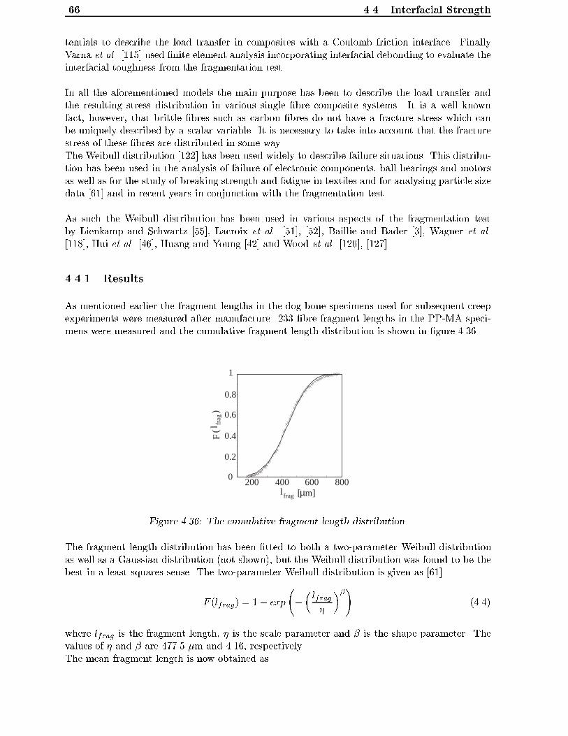
66 4.4. Interfacial Strength
tentials to describe the load transfer in composites with a Coulomb friction interface. FinallyVarna et al. [115] used �nite element analysis incorporating interfacial debonding to evaluate theinterfacial toughness from the fragmentation test.
In all the aforementioned models the main purpose has been to describe the load transfer andthe resulting stress distribution in various single �bre composite systems. It is a well knownfact, however, that brittle �bres such as carbon �bres do not have a fracture stress which canbe uniquely described by a scalar variable. It is necessary to take into account that the fracturestress of these �bres are distributed in some way.The Weibull distribution [122] has been used widely to describe failure situations. This distribu-tion has been used in the analysis of failure of electronic components, ball bearings and motorsas well as for the study of breaking strength and fatigue in textiles and for analysing particle sizedata [61] and in recent years in conjunction with the fragmentation test.
As such the Weibull distribution has been used in various aspects of the fragmentation testby Lienkamp and Schwartz [55], Lacroix et al. [51], [52], Baillie and Bader [3], Wagner et al.[118], Hui et al. [46], Huang and Young [42] and Wood et al. [126], [127].
4.4.1 Results
As mentioned earlier the fragment lengths in the dog bone specimens used for subsequent creepexperiments were measured after manufacture. 233 �bre fragment lengths in the PP-MA speci-mens were measured and the cumulative fragment length distribution is shown in �gure 4.36.
200 400 600 800l frag [ m]µ
0.2
0.4
0.6
0.8
1
0
l frag
()
F
Figure 4.36: The cumulative fragment length distribution.
The fragment length distribution has been �tted to both a two-parameter Weibull distributionas well as a Gaussian distribution (not shown), but the Weibull distribution was found to be thebest in a least squares sense. The two-parameter Weibull distribution is given as [61]
F (lfrag) = 1� exp
��lfrag�
��!(4.4)
where lfrag is the fragment length, � is the scale parameter and � is the shape parameter. Thevalues of � and � are 477.5 �m and 4.16, respectively.The mean fragment length is now obtained as

Chapter 4. Experimental Results 67
hlfragi = ��
�1 +
1
�
�(4.5)
where � is the gamma function and the value of the mean fragment length is hlfragi = 434 �m.
From the �gure it is seen that the two-parameter Weibull distribution describes the �bre fragmentlengths best at intermediate lengths. For small and large �bre fragment lengths the Weibull dis-tribution deviates slightly from the experimental data. This e�ect is easier seen if ln(� ln(1�F ))is plotted against ln(
lfrag:df
) as shown in �gure 4.37.
3210-1-2-3-4-5-63 4 5
ln(-
ln(1
-F))
ln(l /d )frag. f
Figure 4.37: Weibull distribution of �bre fragment aspect ratios.
This deviation have been pointed out by several investigators including Huang and Young [42] intheir investigation of PAN and pitch-based �bres.
In the traditional fragmentation analysis the critical fragment length can now be found as 4/3times the mean fragment length, but Lacroix et al. [51] have shown that the critical length is notalways a material parameter but it depends on the load transfer model used and Feillard et al.[26] concludes that there exists no analytical relationship between the mean fragment length andthe critical length. With these �ndings in mind, the mean fragment length is used as an inputparameter in the following determination of the interfacial shear strength.
The Weibull distribution of �bre strength has mostly been used to simulate the tensile stressesof brittle �bres but Melanitis and Galiotis [64], and Wood et al. [126],[127], have investigatedthe compressional behaviour and the compressional fragmentation of carbon �bres, respectively.Melanitis and Galiotis used a bending rig for the compression tests of HM carbon �bres andfound a strain to break of 0.45 %� 0.05, regardless of �bre length.
The assumption made by Kelly and Tyson regarding yielding in the interface has been ques-tioned by Piggott [82], [83], [84] who claims that yielding at the interface does not occur. Theseconclusions are made on the basis of a Cox model, the rule of mixtures and macroscopic tensiletests.He also suggests that a new failure process should be considered since polymers do not fail inshear but in tension at 45� to the shear plane, [80], [81].
In the present analysis, however, it is assumed that the maximum interfacial shear stress canbe regarded as a constant due to either yielding or as a result of the viscoelastic nature of the
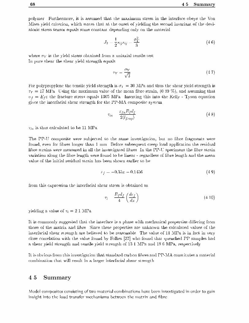
68 4.5. Summary
polymer. Furthermore, it is assumed that the maximum stress in the interface obeys the VonMises yield criterion, which states that at the onset of yielding the second invariant of the devi-atoric stress tensor equals some constant depending only on the material
J2 =1
2sijsij =
�2Y3
(4.6)
where �Y is the yield stress obtained from a uniaxial tensile test.In pure shear the shear yield strength equals
�Y =�Yp3
(4.7)
For polypropylene the tensile yield strength is �Y = 30 MPa and thus the shear yield strength is�Y = 17 MPa. Using the maximum value of the mean �bre strain, (0.39 %), and assuming that�f = Ef" the fracture stress equals 1365 MPa. Inserting this into the Kelly - Tyson equationgives the interfacial shear strength for the PP-MA composite system
�iu ="fuEfdf2hlfragi (4.8)
�iu is thus calculated to be 11 MPa.
The PP-U composite were subjected to the same investigation, but no �bre fragments werefound, even for �bres longer than 1 mm. Before subsequent creep load application the residual�bre strains were measured in all the investigated �bres. In the PP-U specimens the �bre strainvariation along the �bre length were found to be linear - regardless of �bre length and the meanvalue of the initial residual strain has been shown earlier to be
"f = �0:35x � 0:1456 (4.9)
from this expression the interfacial shear stress is obtained as
�i =Efdf4
�d"fdx
�(4.10)
yielding a value of �i = 2.1 MPa.
It is commonly suggested that the interface is a phase with mechanical properties di�ering fromthose of the matrix and �bre. Since these properties are unknown the calculated values of theinterfacial shear strength are believed to be reasonable. The value of 11 MPa is in fact in veryclose correlation with the value found by Folkes [27] who found that quenched PP samples hada shear yield strength and tensile yield strength of 13.1 MPa and 18.6 MPa, respectively.
It is obvious from this investigation that standard carbon �bres and PP-MA constitutes a materialcombination that will result in a larger interfacial shear strength.
4.5 Summary
Model composites consisting of two material combinations have been investigated in order to gaininsight into the load transfer mechanisms between the matrix and �bre.

Chapter 4. Experimental Results 69
Various loading histories have been applied since the loading history by itself may have an in u-ence on the load transfer quality.
The model composites consisting of plasma treated �bres and unmodi�ed polypropylene, (PP-Ucomposites), have been shown to display a friction-like load transfer. Due to the linearity ofthe measured �bre strains it was expected that the load transfer in the PP-U model compositeswas not due to a perfect bonding between the �bre and matrix. This was expected because theinitial elastic �bre strains are very similar even for di�erent applied loads and for loads of 7 MPathe �bre strains are close to zero. Additionally, the initial residual �bre strain showed a lineardependence of the longitudinal �bre co-ordinate.
Di�erent loading histories did not show pronounced di�erences which lead to the conclusionthat the load transfer mechanism has frictional character since viscoelastic e�ects present in thematrix material do not alter the �bre strains during creep loading conditions.Furthermore, the results indicate that the magnitude of the load transfer between the matrixand �bre reached a saturation level governed by the initial residual stresses and the coe�cient offriction.
For longer loading times the �bre creep strains were shown to be very close to zero, indicat-ing that a PP-U composite will not perform as intended, which is also supported by observationsof �bre pull-out.
SEM micrographs were taken of the plasma treated �bres and these investigations revealed someof the reasons for the poor interfacial quality. The �bres have a relatively smooth surface whichsuppresses mechanical interlocking. Finally, the interfacial shear strength was calculated frommeasured �bre strains and found to be 2.1 MPa.
The other material combination consisting of �bres with a standard surface treatment embeddedin a polypropylene matrix grafted with maleic-anhydride, (PP-MA composites). These modelcomposites displayed a much more e�cient load transfer. In fact the load transferred per mil-limeter �bre length is 3 times higher than in the PP-U composites. Also the maximum initialresidual strains are 1.5 times larger than the initial residual �bre strain in the PP-U composites,which corresponds to -0.39 % which is close to the compressive fracture strain found by otherinvestigators. The various measurements on the PP-MA composites showed that the initial resid-ual �bre strains along with the apparently strong interface has a strong restricting e�ect on the�bre strains during creep. This manifests itself in the fact that the load has to be larger than 4MPa for the �bre strain to be tensile after 3 hours of creep.Some of the �bre strains showed pronounced linearity with respect to the longitudinal �bre co-ordinate which is attributed to shear yielding at the interface. This has also been reported byother authors along with the interesting fact that for increasing loading times the �bre straindecreases. This e�ect have been observed in the present investigation as well. This is due tothe fact that when the applied strain increases, more stress is transferred from the matrix to the�bre. Therefore the tensile stress in the �bre increases. However, on further application of load,the matrix yields and is less e�cient in transferring load to the �bre, thus causing the tensilestress in the �bre to decrease.
Fibre misalignment has been considered and it was found that the �bre strain decreases to-wards values smaller than the initial residual strain as the misalignment angle increased. This isassumed to be due to two mechanisms. First the loading condition itself. As the misalignmentangle increases the transverse loading of the interface increases, reducing the e�ect of the radialpressure and thus the amount of load transferred to the �bre. Secondly, the Poisson contribution

70 4.5. Summary
to the longitudinal strain is increased as the misalignment angle increases and when the �bre isorthogonal to the loading direction it will experience compression only.
Preliminary investigations of �bre interaction have been undertaken. Although the results arepreliminary it seems that the interaction distance is much smaller than in the elastic case. Fur-thermore, it seems that interaction is very dependent on �bre arrangement. This suggests thatinteraction between �bres is even more complicated when the response of the investigated modelcomposite is not linear elastic.
SEM micrographs were taken and the �bre surface was found to be much more rough than theplasma treated �bres thus enhancing mechanical interlocking which combined with the maleic-anhydride yields a stronger interface. The interfacial shear strength has been calculated from theKelly-Tyson equation together with the mean fragment length and was found to be 11 MPa, ormore than �ve times as strong as for the PP-U composites.

Chapter
5
Single Fibre Creep Modelling
This chapter describes two approaches to modelling the stress and strain �elds due to one�bre in a viscoelastic matrix material. The �rst one is partly theoretical and partly exper-
imental, i.e. the strains obtained from experiments are used as input to a theoretical approachdescribing the matrix strains at the instant of time when the �bre strains were measured. Thesecond approach is purely theoretical and incorporates the e�ect of thermal stress induced in thespecimen after manufacture.
When a solid is used in a situation which may involve signi�cant loading and deformation itis essential that adequate design should be included in the manufacture of the component.This may be necessary to ensure e�cient material utilisation, to prevent unacceptable deforma-tion during service or to avoid failure of the component. In part these design requirements can bemet by providing methods for stress and deformation analysis for the relevant material behaviour.Essentially this requires some form of theory to model the behaviour, experimental techniquesfor measuring the material parameters, and methods for calculations relevant to the application.Obviously the degree of sophistication employed will be governed by the application and themethods of calculation may involve detailed mathematical or numerical analysis or the use ofsimpli�ed engineering theories. Whatever method is employed the theoretical basis and experi-mental data should have a corresponding degree of sophistication.
Due to the fact that only one component of the �bre strain is measured by Raman spectroscopythere would be a sophistication discrepancy between the experimental data and the theoreticalmodelling if a highly sophisticated model were used. On this basis two simpler but adequateapproaches will be proposed in this chapter.
Since the matrix is the load transferring media, it is crucial that a theoretical model describesthe �eld quantities in the matrix properly. It is important to have an adequately qualitativedescription of the �eld quantities in order to improve the overall performance of the composite,e.g. optimise the creep strength by enhancing interfacial properties and to understand the mech-anisms of the load transfer.
The main objective in the present study is to investigate the localised phenomena from a mi-cromechanical point of view.Similar investigations using various approaches have been undertaken by other researchers, suchas Pachalis and Chou [76] who developed a model for predicting the steady-state creep behaviour
71

72
of misaligned short-�bre reinforced ceramic matrix composites. Their model is based on an ad-vanced shear-lag model. One of the major assumptions in their analysis is that there is no stresstransfer from the matrix to the �bre at the �bre end surface.The authors analyses the e�ect of �bre orientation and the e�ect of the coe�cient of slidingfriction between the matrix and the �bre.It is shown that the creep rate increases - with increasing orientation angle - until the �bre orien-tation angle reaches about 60 degrees, relative to the loading axis, where the creep rate reachesan asymptotic value. At low values of the coe�cient of sliding friction the composite behaves asa pure matrix with holes.No experimental data for comparison or validation of their model have been shown.
S�rensen [111], investigated the creep behaviour of short �bre reinforced metal-matrix compos-ites. The experimental work included creep tests and neutron di�raction tensile tests at elevatedtemperatures, performed on SiC-whisker reinforced aluminium. Calculations were carried outusing �nite elements.In the numerical analysis the �bres were assumed to be perfectly bonded to the matrix material.Using a hyperbolic sinusoidal creep law S�rensen analysed the e�ects of inclusion shape and �bremisalignment. It was found that for inclusions of circular cross section the volume fraction has tobe approximately twice that of a square cross section �bre to give the same creep resistance. Themisalignment of the �bres gives rise to a lower creep resistance due to the lower constraining ofthe �bre on the matrix. Furthermore, it is seen that the larger misalignment the larger rotationof the �bres towards a parallel position.Comparison of experimental results with numerical calculations show that the stresses found inthe experiments are larger than the those predicted by the model. This might be caused bydislocation-particle interaction, (e.g. Orowan looping), and that the oxide particles in the alu-minium powder serve as barriers to dislocation movements.
Goto and McLean [33], developed a shear lag-like model and used it to analyse the e�ect ofvarious interfaces on the creep behaviour in metal-matrix composites.It was assumed that the matrix deformation obeys power law creep and that no load is transmit-ted along the �bre ends. By applying the rule of mixtures the creep rate of a unit cell, containingone �bre, was obtained. Introducing an interface of thickness, �, enables the description of thecreep rate in terms of a parameter which can be regarded as describing the creep strength of theinterface. According to the authors there are only very few results against which this model canbe validated.The principal prediction from this model is that the interface strength in uences the creep be-haviour strongly, meaning that if the interface has no strength, the creep resistance of the com-posite is lower than that of the pure matrix. Furthermore, the creep performance is sensitive to�bre aspect ratio and �bre volume fraction.
Song et al. [109], analyses continuous �bre reinforced ceramic- and metal-matrix composites.A cylindrical cell model was considered. This cell model consists of one broken �bre which isin uenced by six intact surrounding �bres. The matrix is assumed to obey power law creep andthe �bres are assumed to be isotropic linear elastic and perfectly bonded to the matrix. Thecalculations are carried out using �nite elements.It was found that the presence of the broken �bre has great in uence on the creep strain rate. Ifbroken �bres are present the creep strain rate does not stabilise, not even after very long time.Creep strains are concentrated at the crack tip region and the creep zone expands with time,primarily along the �bre-matrix interface. This is caused by the large shear stress induced bythe crack in the interface. This may cause interface sliding and have a pronounced e�ect on therelaxation of the matrix stresses. No experimental results for veri�cation are shown, but the

Chapter 5. Single Fibre Creep Modelling 73
model is compared to other models and shows reasonable agreement.
Wang and Chou [121], proposed a model based on advanced shear lag theory. The shear lagapproach is applied to a unit cell containing one �bre, which can be \misaligned" by an angle �relative to the loading axis.It is assumed that both the �bre and the matrix creep but at di�erent rates. Both phases areassumed to carry axial and shear loads. Furthermore, sliding along the interface is considered anda sliding factor is incorporated in the analysis. Power law creep is assumed for uniaxial tensionand the Prandtl - Reuss ow rule used in order to account for three dimensional stress states. Alinear distribution of the interfacial shear stress is assumed and the rule of mixtures is applied tosolve the problem.Numerical calculations show that the longitudinal creep strain rates with perfect and no bondingare 31 % and 80 % of the pure matrix, respectively.The longitudinal creep controls the unit cell when the �bre \misalignment angle" is less than15�, the shear creep becomes dominant when � is between 15� and 75�, and the transverse creepcontributes mostly to the creep strain rate when the angle is larger than 75�. When the inter-facial sliding factor becomes high, (weak bonding), the resistance to shear and transverse creepdiminishes.
5.1 Creep Modelling, Approach I
In this section a semi - theoretical approach is outlined in order to describe the local matrixcreep strains and has also been used in Schj�dt-Thomsen and Pyrz [104]. The approach is semi- theoretical, i.e. it uses experimental results as an input parameter for the modelling and thusthe creep strains are only obtained at a loading time corresponding to the time, during the ex-periment, at which the measurement was conducted.This approach is inspired by Fukuda and Kawata [28]. They used the concept of point forces inan in�nite plate to investigate the elastic stresses and strains in a composite with a regular arrayof �bres. The interfacial tractions for one �bre due to an externally applied load are calculated.These tractions are integrated along the boundary of the �bre, thereby giving the stresses in thematrix material.In Fukuda and Kawata's analysis it is assumed that the stresses and strains are identical for allthe �bres in the array. For one �bre the results obtained are quite good compared to experiments.
The present approach di�ers from Fukuda and Kawata's by incorporating the actual variationof interface tractions along the �bre boundary, as obtained through force equilibrium at the in-terface based on the �bre strains from the MRS investigations. The interfacial stresses alongthe �bre are obtained from the actual �bre strain at various times. The interfacial stresses arethen integrated along the �bre boundary giving the stresses in the matrix material. The matrixstresses are then inserted into the three dimensional constitutive equation of the matrix, thusgiving the creep strain distribution in the matrix material around the �bre. Additionally, thismodel is able to consider misalignment of the �bre.
Pointforces
In modelling the forces acting on the interface between the �bre and the matrix material, onlythe interfacial shear stress, ��xy, and the transverse normal tractions, ��y, are considered.
The stresses in the matrix, �(1)ij , due to the applied load, �1IJ , are given by

74 5.1. Creep Modelling, Approach I
σ 8
σ 8
x
yX
X
X
Yθ
Figure 5.1: The �gure shows the loading situation.
8>><>>:�(1)x
�(1)y
�(1)xy
9>>=>>; =
264 m2 n2 2mn
n2 m2 �2mn�mn mn (m2 � n2)
3758><>:
�1X�1Y�1XY
9>=>; (5.1)
where capital letters refer to the global coordinate system. m = cos �, n = sin � and � is theangle between the �bre x axis and the global X axis, as shown in �gure 5.1.
From Timoshenko [113], it is known that a force, P , acting in the x-direction at a point (x0; y0)in an in�nite plate creates the stresses �x(x; y), �y(x; y) and �xy(x; y) given by
�x(x; y) =P
4�
(x� x0)
(x� x0)2 + (y � y0)2
(�(3 + �) + 2(1 + �)
(y � y0)2
(x� x0)2 + (y � y0)2
)
�y(x; y) =P
4�
(x� x0)
(x� x0)2 + (y � y0)2
((1� �)� 2(1 + �)
(y � y0)2
(x� x0)2 + (y � y0)2
)(5.2)
�xy(x; y) =P
4�
(y � y0)
(x� x0)2 + (y � y0)2
((1� �) + 2(1 + �)
(x� x0)2
(x� x0)2 + (y � y0)2
)
Equations (5.2) are used to �nd the stresses in the matrix material after rewriting them andreplacing P by the interfacial stresses as
�(2)x (x; y) =1
4�
Z lf=2
0��xy(�)
�(x� x1)
(x� x1)2 + (y � y1)2
�(�(3 + �) + 2(1 + �)
(y � y1)2
(x� x1)2 + (y � y1)2
)+
(x� x1)
(x� x1)2 + (y � y2)2
�(�(3 + �) + 2(1 + �)
(y � y2)2
(x� x1)2 + (y � y2)2
)� (x� x2)
(x� x2)2 + (y � y1)2(5.3)
�(�(3 + �) + 2(1 + �)
(y � y1)2
(x� x2)2 + (y � y1)2
)� (x� x2)
(x� x2)2 + (y � y2)2
�(�(3 + �) + 2(1 + �)
(y � y2)2
(x� x2)2 + (y � y2)2
)#d�

Chapter 5. Single Fibre Creep Modelling 75
where x1, x2, y1, and y2 are given by
x1 = x0 + �
x2 = x0 � �
y1 = y0 + df=2
y2 = y0 � df=2
For convenience only the stress in the x-direction due to the interfacial shear stress is shown here,since the others are analoguous. The expressions for the remaining components can be found inappendix A. After carrying out the integrations the stress �eld in the matrix material due to thepresence of the �bre is obtained. The stresses in the matrix material due to the applied load,
the interfacial shear stress and the transverse normal tractions are denoted as �(1)ij , �
(2)ij and �
(3)ij ,
respectively.
σ σ
σ σ
σf f f
d+
τ i
fibredx
x
y
dx
app. app.
Figure 5.2: The free body diagram of the �bre.
The interfacial shear stress excerted on the �bre is obtained by equilibrating forces as shown in�gure 5.2 and the equilibrium equation for the �bre becomes
dfd�f (x)
dx� 4��xy(x) = 0 (5.4)
where df is the �bre diameter.Expressing the �bre stress �f as El
f"f the interfacial shear stress can be stated as
��xy(x) =dfE
lf
4
d"fdx
(5.5)
where "f is the �bre strain obtained from experiments.In some situations the �bre strain distribution may be linear. This linear distribution may occurwhen interfacial debonding is present, [43], if the load transfer mechanism is governed by friction,[48], [53] or if shear yielding occurs, [49]. In the previous chapter it was shown that the loadtransfer mechanism in the PP-U model composites is governed by the initial residual stress andthe coe�cient of friction. This friction is assumed to be Coulomb friction and thus the followingrelation is assumed to be valid
��xy(x) = ��fric��y(x) (5.6)

76 5.1. Creep Modelling, Approach I
where �fric is the coe�cient of friction.
z
r
2a2bθ
Figure 5.3: Coaxial cylinders used in the Lam�e solution.
The initial transverse traction is a radial pressure due to manufacture of the specimen and can beobtained from the Lam�e solution, see e.g. [12]. The Lam�e solution is obtained by assuming thatthe �bre and matrix can be modelled as two coaxial cylinders with radii a and b, respectively,�gure 5.3.
Assuming a displacement �eld of the form
ur = f(r) u� = 0 uz = C0z (5.7)
where u� = 0 due to symmetry. Inserting the assumed displacement �eld into the only non-vanishing equilibrium equation (the remaining equilibrium equations are identically satis�ed dueto rotational symmetry and due to the in�nite length of the �bre/matrix cylinder)
@�r@r
+�r � ��
r= 0 (5.8)
gives a second order di�erential equation of the form
@2ur@r2
+1
r
@ur@r
� urr2
= 0 (5.9)
which is solved subject to the following conditions
� Radial stresses in the matrix are zero at r = b, i.e. �mr (b) = 0.
� Continuity of stress at the interface, i.e. �fr (a) = �mr (a).
� Equilibrium of forces at the composite cylinder cross section, �fzAf + �mz Am = 0.
The radial stress in the matrix is then obtained as
�mr =k4(�m � �lf ) + k2(�
tf � �m)
k1k4 � k2k3
1� b2
r2
!�T (5.10)

Chapter 5. Single Fibre Creep Modelling 77
where the constants ki are given by
k1 = 2
�mEm
+�lf
Elf
1� �
�
!
k2 = �
1
Em+
1
Elf
1� �
�
!
k3 = �1� �mEm
� 1 + �mEm
1
�� 1� �tf
Etf
1� �
�
k4 =�mEm
+�lfElf
1� �
�
where Em and �m are Young's modulus and Poisson ratio of the matrix respectively. �m, �lf , �
tf
are coe�cients of thermal expansion of the matrix and coe�cients of thermal expansion in thelongitudinal and the transverse direction of the �bre respectively. El
f and Etf are Young's moduli
of the �bre in the longitudinal and transverse direction respectively. �lf and �tf are the Poissonratios in the longitudinal and transverse direction respectively. � is the ratio of the squareddiameters of the �bre and matrix, respectively and given as � = a2=b2. �T equals the di�erencebetween the crystallisation temperature and ambient temperature. For cooling rates of � 100�C=min, DSC measurements have shown that the crystallisation temperature is � 103 �C [73].Combining equations (5.5), (5.6) and (5.10) the coe�cient of friction is found to be �fric = 0.21.The resulting stresses in the matrix material are now obtained by a simple superposition of the
three contributions, �(1)ij , �
(2)ij and �
(3)ij . These stresses and the appropriate time are inserted into
the constitutive law of the matrix material, equation (3.31), and then the matrix creep strainscan be found.
5.2 Creep Modelling, Approach II
In this section a theoretical approach is described from which the stress and strain in the matrixmaterial can be obtained at any desired time. This approcah is an extension of the method justshown and results from this approach can also be found in the papers by Schj�dt-Thomsen andPyrz [105] and [106].The approach is inspired by a paper by Argon [2]. On the basis of Eshelby's thought experimentthe elastic stress and strain in a composite consisting of one short �bre embedded in an in�nitematrix are calculated. The �bre and matrix are linearly elastic isotropic and assumed to haveidentical Poisson's ratios and only load applied parallel to the �bre axis is considered.
In the present analysis the stress and strain during creep are calculated using Eshelby's thoughtexperiment and an incremental stress/strain formulation of the Schapery model. Furthermore,o� - axis loading, di�erent Poisson's ratios, transversely isotropic �bres as well as thermal e�ectsare considered.
An exact solution to the problem of a cylindrical �bre of �nite length embedded in an in�-nite matrix is very di�cult to obtain but a usefull and reasonably accurate solution is obtainableby means of Eshelby's thought experiment. Eshelby originally used this approach to model thestress/strain �eld due to martensitic formation in metals. He solved the problem in the followingelegant way.

78 5.2. Creep Modelling, Approach II
Cut the inclusion from its surrounding matrix. Allow the inclusion to transform. Apply sur-face tractions which restore the inclusion to its original form, put it back in the matrix and rejointhe material across the cut. The stress is now zero in the matrix and has a known constantvalue in the inclusion. The applied surface tractions have become built in as a layer of bodyforce spread over the interface between the inclusion and matrix. To complete the solution thisunwanted layer is removed by applying an equal and opposite layer of body force. The additionalelastic �eld thus introduced is found by integration from the expression for the elastic �eld of apointforce, [24].
This approach gives the initial elastic stresses in the matrix. Inserting the initial stresses intothe three dimensional constitutive law of the matrix, equation (3.31), gives the initial elasticstrains. These strains give rise to stress relaxation during a small amount of time, dt. The stressrelaxation during time dt creates a new state of stress which is used to calculate the strains forthe next time increment etc.
A transversely isotropic �bre of length lf and diameter df is embedded in an in�nite initiallyelastic matrix with Youngs modulus Em and Poisson's ratio �m. The system is subjected totensile stresses �1IJ at the remote boundary. If the �bre is misaligned with respect to the loadingaxis the applied stress is transformed into the �bre co-ordinate system through equation (5.1),thus �1x , �1y and the interfacial shear stress can be determined.
To �nd the initial stress in the matrix the �bre is removed from the in�nitely extended ma-trix and replaced by matrix material. �1x , �1y and a temperature change, �T, are applied,causing strains "1x and "1y . The matrix material occupying the position of the �bre is removedand surface tractions, �1x and �1y are placed along the boundary of the \hole", as shown in �gure5.4A.
A B
σ 8
x
σ 8
x
σ 8
x
σ 8
x
σ 8
yσ 8
y σ 8
yσ 8
y
x
8ε Efl 8εy Ef
t νl-f
8εy Eft
x
8ε Efl νt-
f
Figure 5.4: Tractions A) on the matrix and B) on the �bre.
Tractions of magnitude "1x Elf are applied to the ends of the �bre and "1y E
tf are applied to the
sides of the �bre in order to make it �t perfectly into the deformed hole of the matrix. The trac-tion applied to the end of the �bre causes additionally transverse stresses of magnitude ��tf"1x El
f .
Furthermore the transverse traction, "1y Etf , causes a longitudinal stress of magnitude �"1y Et
f�lf ,
�gure 5.4B. The additional longitudinal stress will make yet another contribution to the trans-verse stress but this is neglected since it contains higher order terms of the Poisson's ratios, such

Chapter 5. Single Fibre Creep Modelling 79
as �m�lf .
The interfacial tractions in the composite when the �bre is put back into the matrix are nowreadily obtained as
��x = ��1x +�1xEm
Elf �
�1yEm
Etf�
lf + �m�T (E
tf�l �El
f )
��y = ��1y +�1yEm
Etf �
�1xEm
Elf�
tf + �m�T (E
tf �El
f�t) (5.11)
In this equation the only thermal contributions are due to the matrix. The contributions fromthe �bre are neglected since �m � �f .If the tractions in equation (5.11) are used as they are and applied directly to the matrix at theinterface they will cause an incompatible displacement �eld. So in order to ensure compatibilityand to determine the interfacial forces to be integrated along the �bre boundary it is necessaryto determine the fraction of force which is carried by the �bre and matrix, respectively. This isdone by combining the stress-strain relations and the strain-displacement relations as
@ux@x
=1
E0
m
��x � � 0m�y
� @uy@y
=1
E0
m
��y � � 0m�x
�(5.12)
where E0
m and � 0m depends on whether the deformation state is plane stress or plane strain andare given by
E0
m =
(Em plane stressEm
1��2mplane strain
� 0m =
(�m plane stress�m
1��mplane strain
where the plane strain assumption is used in this approach.
Both ux and uy consist of two contributions; one from the longitudinal interfacial tractions andone from the transverse interfacial tractions. The stresses in the matrix material due to thesetractions are obtained by rewriting equations (5.2) as
�x(x; y) =Px4�
( (x+ lf=2)
(x+ lf=2)2 + (y)2
! �(3 + �) + 2(1 + �)
(y)2
(x+ lf=2)2 + (y)2
!
�
(x� lf=2)
(x� lf=2)2 + (y)2
! �(3 + �) + 2(1 + �)
(y)2
(x� lf=2)2 + (y)2
!)
�y(x; y) =Px4�
( (x+ lf=2)
(x+ lf=2)2 + (y)2
! (1� �)� 2(1 + �)
(y)2
(x+ lf=2)2 + (y)2
!
�
(x� lf=2)
(x� lf=2)2 + (y)2
! (1� �)� 2(1 + �)
(y)2
(x� lf=2)2 + (y)2
!)(5.13)
�x(x; y) =Py4�
( (y + df=2)
(x)2 + (y + df=2)2
! (1� �)� 2(1 + �)
(x)2
(x)2 + (y + df=2)2
!
�
(y � df=2)
(x)2 + (y � df=2)2
! (1� �)� 2(1 + �)
(x)2
(x)2 + (y � df=2)2
!)

80 5.2. Creep Modelling, Approach II
�y(x; y) =Py4�
( (y + df=2)
(x)2 + (y + df=2)2
! �(3 + �) + 2(1 + �)
(x)2
(x)2 + (y + df=2)2
!
�
(y � df=2)
(x)2 + (y � df=2)2
! �(3 + �) + 2(1 + �)
(x)2
(x)2 + (y � df=2)2
!)
which correspond to the stresses in an in�nite plane due to a point force in the x-direction at(x; y) = (�lf=2; 0) and a point force in the y-direction at (x; y) = (0;�df=2), respectively. Nowux and uy are readily found by inserting these stresses into the stress-displacement relations givenin equations (5.12). The displacements are now obtained as functions of both x and y as
ux = f(x; y) + h(y) uy = g(x; y) + q(x) (5.14)
where h(y) and q(x) are arbitrary functions due to the integration. h(y) and q(x) need to be zeroin order to keep ux and uy symmetric about x = 0 and y = 0, respectively.The displacements ux and uy are singular for (x; y) = (�lf=2; 0) and (x; y) = (0;�df=2). Todetermine the fraction of force carried by the �bre and the matrix it is necessary to de�ne averagedisplacements across the �bre end, huxi, and along the sides of the �bre, huyi, as
huxi = 2
df
Z df=2
0uxdy
huyi = 2
lf
Z lf=2
0uydx
These average displacements are non-singular at x = �lf=2 and y = �df=2. huii are of the form
huii = � P
8�Emdf
nf(�m; df ; lf ); tan
�1(df ; lf )o
(5.15)
huxi and huyi gives the average displacements due to a force P and can be rearranged to give thedisplacement due to a unit force dP . The relation between the displacements huxi and huyi andthe unit force dP can be thought of as being the sti�ness of the in�nite medium in the x- andy-direction, respectively. These sti�nesses are obtained as
Kmx =
dP
dhuxi Kmy =
dP
dhuyi (5.16)
The sti�nesses of the �bre in the x- and y-direction are calculated as
Kfx =
dfElf
lfKfy =
lfEtf
df(5.17)
Now the sti�nesses of the matrix and the �bre are used to determine the fraction of the interfacialforce carried by the �bre and matrix, respectively. The fraction of the force carried by the matrixin the x- and y-direction are denoted as �Pm
x and �Pmy and are determined as
�Pmi = Km
i �ui

Chapter 5. Single Fibre Creep Modelling 81
where �ui are given as
�ux = � ��xdf
Kmx +Kf
x
�uy = � ��ylf
Kmy +Kf
y
(5.18)
The �nal interfacial tractions to be integrated along the �bre boundary are now found to be
�int:x = � ��xKmx
Kmx +Kf
x
�int:y = � ��yKmy
Kmy +Kf
y
(5.19)
If the �bre is misaligned the interfacial shear stress is found using equation 5.1, inserted into the�rst of equation 5.19 replacing ��x and �nally integrated using the expressions in appendix A.
Creep Strains
The disturbed stress �eld is obtained by integrating the tractions along the �bre boundary andinserting the resulting matrix stresses into the three dimensional constitutive law of the matrixfor t = 0, thus giving the initial elastic strain disturbance. This strain causes stress relaxationduring a time step dt, resulting in a new state of stress �ij + d�ij to be used in the next timeincrement together with t = dt, causing a new state of strain which again causes stress relaxationand so on. This is repeated until t is equal to the desired time of duration.In order to do that the incremental stresses and strains are needed. The incremental strains arefound by di�erentiating equation (3.31) and are given as
d"ij(t) = f(1 + �m)�ij � �m�kk�ijg @~D(t)
@tdt (5.20)
where it is assumed that the stresses are constant during the time increment dt. The time varyingstresses are obtained in the same manner as
d�ij(t) =1
1 + �m
�"ij +
�m1� 2�m
�ij"kk
�@ ~E(t)
@tdt (5.21)
where it is assumed that the strains are constant during the time increment.To calculate the creep strains around the �bre the following procedure is now applied:
1. Calculate the initial matrix stresses, �0ij , from the tractions.
2. Insert the initial stresses into equation (3.31) together with time, t = 0, thus givingthe initial elastic strains, "0ij .
3. Insert the initial strains into equation (5.21), thus giving d�ij(t).
4. �ij(t) = �0ij + d�ij(t).
5. Insert �ij(t) and the appropriate time into equation (5.20), thus giving the incrementalstrain, d"ij(t).
6. "ij(t) = "0ij + d"ij(t).

82 5.3. Finite Element Analysis
7. Insert the \new" strain "ij(t) and appropriate time into equation (5.21).
8. Repeat step 3 to 7 until t equals the desired time.
9. Add the far�eld stress and strain to obtain the complete solution.
5.3 Finite Element Analysis
Nonlinear �nite element models are considered in this section. Only models with �bres alignedalong the loading direction are analysed by FEM, in order to treat the models axisymmetrically.The program used is the commercial FE program, COSMOS/M.
The main purpose of the FE - analysis is to do further checking of the frictional load trans-fer assumption and the apparent yielding in the interface between the �bre and matrix.
Finite element analysis combined with Raman spectroscopy has not been widely used in spiteof the fact that this is a suitable combination for investigating the complex stress/strain statesurrounding the �bres in short �bre reinforced composites.Although some investigations have dealt with FEM, it seems that the e�ects of both nonlinearityand thermal history are neglected in these analysis.
Fan and Hsu [25] investigated the e�ect of �bre end shapes on load transfer e�ciency in thelinear elastic case. They found that a blunt end would cause much higher stresses in the vicinityof the �bre than a tapered end, which might lead to premature failure, whereas �bres with ta-pered ends enhance the load transfer e�ency due to the constant level of stress in the �bre. Agood agrement is found between FE analysis and Raman experiments, for both kind of �bre ends.
Guild et al. [37] investigated the stress transfer in model composites by both Raman spec-troscopy and FEM. The FE model incorporates the e�ect of matrix plasticity. It is concludedthat plasticity has a pronounced e�ect on the load transfer. Two �bre geometries are considered.One with a rounded end and one with sharp corners at the end. Comparison between Ramanmeasurements and these two geometries show generally good agreement but since the Ramanresults di�ers from the FE results in the case of sharp �bre corners, the authors conclude thatthis �bre geometry should not be used in the FE models since on a molecular level all cornersare rounded.
Scha�er and Adams [98] used the nonlinear single-integral constitutive equations developed bySchapery in their FE analysis of a unidirectional composite subjected to transverse loading. Theyfound a good agreement with experimental results in the case of uniaxial loading.
The present analysis di�ers from those mentioned above because the e�ect of thermal residualstrains and stresses on subsequent creep strains are accounted for in the FE model. Furthermore,matrix plasticity and frictional load transfer at the interface is considered.
The FE Models
The models are considered as being axi-symmetric and thus only one quarter of the cross sec-tion of the model is considered. The models considering the PP-U model composites have outerdiameters of 80 �m, whereas the models considering the PP-MA model composites have outer

Chapter 5. Single Fibre Creep Modelling 83
diameters of 130 �m. The diameters corresponds to twice the thickness of the polypropylene �lms.
The �nite element meshes used for the PP-U and PP-MA model composites are shown in �gures5.5A and 5.5B, respectively. The �bre is modelled as being transversely isotropic. The �brediameters for the plasma treated �bre and the standard surface treated �bre were measured inthe previous chapter and were found to be 6.1 �m and 6.7 �m, respectively. The �bre diameterin the FE models are taken to be the same in each case at 6.5 �m. The �bre length modelled inboth cases corresponds to the mean �bre length, i.e. 740 �m and 450 �m, respectively.
z,(x)
r,(y)A
z,(x)
r,(y)B
Figure 5.5: The FE mesh used for A) the PP-U model composites and B) the PP-MA model com-posites. Letters in parenthesis corresponds to the directions used in the theoretical
approaches.
The elements used in the analysis are 4 and 8 node isoparametric elements. In the mesh usedfor the PP-MA FE models, �gure 5.5B, there are in fact 4 times as many elements as shown.However, a �gure with the correct number of elements is nearly totally black and is therefore notshown. Using this small element size enables the plotting of matrix �eld quantities at a radialdistance of 1 �m from the �bre surface. In the PP-U FE models the interfacial quantities areplotted along the �bre matrix boundary, because in this situation the material properties are not"mixed" along the �bre/matrix interface.
Thermal loading
To incorporate the e�ect of thermal history upon subsequent loading it is necessary to simu-

84 5.3. Finite Element Analysis
late the cooling process of the material. This is done by subjecting all the nodes in the modelto a uniform temperature of 103 �C at the beginning of the analysis. The model is then cooleddown to 20 �C in 0.01 hour. The response of the model to subsequent loading will now dependon the thermal history.To apply the thermal and mechanical loading histories, \time-temperature curves" are de�ned.The FE model is then subjected to loading histories corresponding to these time-temperaturecurves. The time-temperature curve for the cooling procedure and subsequent creep loading isshown in �gure 5.6.
T [ C]o σ [MPa]
105
20
0.01 time [hr.]
σappl.
t finish
Figure 5.6: The \time-temperature curves" de�ning the thermal and mechanical loadings in the
FE program.
The e�ect of temperature on Young's modulus of the matrix material is accounted for by de�n-ing a "temperature-property" curve, which is analogous to the time-temperature curves. Young'smodulus as a function of temperature is shown in �gure 5.7. The data has been provided byBASF.
20 40 60 80 100 120
E(T
)[G
Pa]
m
1.6
1.2
0.8
0.4
T [ C]o
Figure 5.7: Variation of Young's modulus with temperature.
The FE program interpolates linearly between the de�ned points to determine the value ofYoung's modulus at a certain temperature.During the cooling process the coe�cients of thermal expansion are assumed to be independentof temperature.

Chapter 5. Single Fibre Creep Modelling 85
Creep constitutive law
The creep modelling in the FE program is based upon a classical power law for creep, the Bailey- Norton law, which describes the uniaxial creep strain as a function of the uniaxial stress, timeand temperature and is expressed as
"c = C0�C1tC2e
(�CT
T+Tref)
(5.22)
where C1 > 0, 0 < C2 < 1, T is temperature, Tref is a stress free temperature and CT is amaterial constant de�ning the creep-temperature dependency.This creep law represents both the transient and the steady creep regime, but does not take intoaccount the elastic response which must be considered when the constants are determined fromexperimental data.
In order to extend this law to multiaxial behaviour the following assumptions are made [110]:
� The uniaxial creep law remains valid if the uniaxial creep strain and the uniaxialstress are replaced by their e�ective values.
� Material is isotropic, i.e. stresses and strains are independent of orientation.
� The creep strains are incompressible, i.e. ecij = "cij
The third assumption enables the use of the Von-Mises ow rule
_"cij =
pK2pJ2sij (5.23)
where K2 and J2 are the second invariants of _ecij , (K2 = 12 _e
cij _e
cij) and the deviatoric stress sij
(J2 = 12sijsij), respectively. This simpli�es the numerical solution procedure and is also the
reason why creep is sometimes called "rate dependent plasticity".
Due to the simplicity of the creep constitutive model and the fact that polypropylene is highlynonlinear it is necessary to use di�erent values of the parameters for each load case. This meansthat C1 in the Bailey - Norton creep law changes slightly as a function of stress, from being 1 at� = 1 MPa to 1.2128 at � = 8 MPa. The experimental data along with the Bailey - Norton lawis shown in �gure 5.8
Frictional Elements
As shown earlier the �bre strain in the PP-U composites show a linear dependence on the axialcoordinate and it has been concluded that the load transfer is governed by friction.
To model frictional phenomena \node-to-node" gap elements are speci�ed along the boundarybetween the �bre and the matrix.Two node gap elements are used in contact problems when two bodies are coming in contact witheach other due to the application of external forces. The main assumption in the modelling ofthis type of element is that the direction of the normal force and the contact points are knownin advance and remain unchanged during the analysis. The two node gap elements are placedbetween two nodes of the contacting bodies (one node on each body) such that the direction of

86 5.4. Results from Approaches I, II and FEM
1.4
1.2
1.0
0.8
0.6
0.4
0.2
00 5 10 15 20
time [hr.]
ε [%
]
Figure 5.8: The experimental data along with the Bailey - Norton creep law.
the gap element - represented by a straight line joining the initial locations of its two nodes -coincides with the direction of the normal contact force, see �gure 5.9. Depending on the typeof contact problems the gap element can be speci�ed to be either a compressive gap (limitingthe relative contraction between nodes) or a tensile gap (limiting the relative expansion betweennodes). Friction can then be considered using compressive gap elements, [110].
o
o
oo
node 1
node 2
n
undeformed
deformed
1'
2'
u1
u2
urel.
FN
FN
Ffric.
Ffric.
Figure 5.9: Two-node gap element.
In the present models the part of the �bre which is in contact with the matrix material is de�nedas the \contact surface" and the matrix is de�ned as the \contactor body". The nodes of thegap are now allowed to move relative to each other until contact between the �bre and matrixis established. After contact the nodes can not penetrate into the �bre and a friction force isdeveloped due to the normal force. Care must be taken when de�ning the gap elements becausea wrong orientation of the elements will cause the �bre to be penetrateable for the nodes.
5.4 Results from Approaches I, II and FEM
In this section some selected results from experiments are compared to results obtained fromboth the two theoretical approaches and FEM.When the interface is \strong" as in the PP-MA model composites, approach II is used. Whenthe interface is weaker and the load transfer is of a frictional character, as in the PP-U modelcomposites, approach I is used.

Chapter 5. Single Fibre Creep Modelling 87
Calculations have been conducted in order to investigate the in uence of the magnitude of thecoe�cient of friction on the stress pro�le in the �bre.Figure 5.10A shows the longitudinal thermal residual stresses in the �bre as a function of thecoe�cient of friction. It is seen from the calculations that for low values of �fric the end e�ect ismore pronounced and contributes more to the magnitude of the �bre stress. For values of �fricof 0.5 and 0.8 the �bre stress shows a pronounced nonlinearity with respect to the longitudinalcoordinate. For even larger values of �fric there is virtually no di�erence in the stress pro�lecompared to the perfectly bonded case, �gure 5.10B. This implies that it is very di�cult to de-termine if the load transfer is frictional or due to an adhesive bond just from the shape of thestrain pro�le obtained from the MRS measurements.
0 100 200 300 400
0
-400
-800
-1200
σf
[MP
a]
L f [ m]µ
µ = 0.2fric
µ = 0.1fric
µ = 0.5fric
µ = 0.8fric
A
0 100 200 300 400-1200
-800
-400
0
σf
[MP
a]
L f [ m]µ
x
x xx
x
xx
perf. bond.
µ =1.0fricx
B
Figure 5.10: A) The thermal residual �bre stress for various values of �fric. B) The thermal
residual �bre stress in the perfect bonded case and in case of a large value of �fric.
In �gure 5.11 the thermal residual �bre stresses from a cooling analysis with Coulomb frictionacting at the interface is shown along with the mean value obtained from the Raman experi-ments and a good agreement between the FEM values and the experimental values is obtained.This good agreement between experiments and modelling veri�es the assumption that the loadis transferred by friction. It is also apparent from the �gure that the zone of in uence from the�bre end is very small, corresponding to a distance of approximately 4 �bre diameters. However,as mentioned before the end e�ect contributes signi�cantly to the magnitude of the �bre stress.
In �gure 5.12 the calculated longitudinal �bre stress is shown along with the measured �brestress. From the �gure it is seen that even though the zone of in uence of the �bre end is smallit has a large e�ect on the �bre stress level. This is also the reason for the discrepancy betweenthe experimental values and the calculated values. The experimentally determined �bre stressis lower than the �bre stress from FEM. The reason is that the �bre end is believed to debondon the application of load, whereas the �bre is perfectly bonded to the matrix in the FE model.However, the linearity of the stress approximately 20 �m away from the �bre end shows a slopevery close to that of the experimental stress, which again veri�es the frictional load transfermechanism.
In �gure 5.13 the interfacial shear stress along with the radial stress are shown. In conjunctionwith the use of the Lam�e solution it is assumed - for the �bre lengths considered here - that the
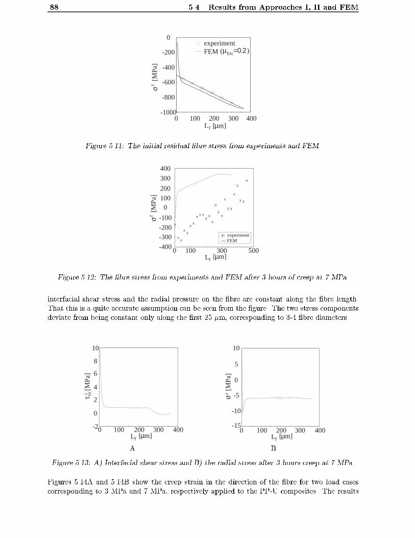
88 5.4. Results from Approaches I, II and FEM
σf
[MP
a]
L f [ m]µ
experimentFEM µ =0.2fric( )-200
-600
-10000 100 200 300 400
0
-400
-800
Figure 5.11: The initial residual �bre stress from experiments and FEM.
0 100 300 500-400
-300
400
-200
-100
0100200
300
Lf [ m]µ
σf
[MP
a]
x: experiment--: FEM
Figure 5.12: The �bre stress from experiments and FEM after 3 hours of creep at 7 MPa.
interfacial shear stress and the radial pressure on the �bre are constant along the �bre length.That this is a quite accurate assumption can be seen from the �gure. The two stress componentsdeviate from being constant only along the �rst 25 �m, corresponding to 3-4 �bre diameters.
Lf [ m]µ-2
0
2
4
6
8
10
0 100 400200 300
[MP
a]τ x
yi
A
Lf [ m]µ0 100 200 300 400
-15
-10
-5
0
5
10
[MP
a]σ
r
B
Figure 5.13: A) Interfacial shear stress and B) the radial stress after 3 hours creep at 7 MPa.
Figures 5.14A and 5.14B show the creep strain in the direction of the �bre for two load casescorresponding to 3 MPa and 7 MPa, respectively applied to the PP-U composites. The results

Chapter 5. Single Fibre Creep Modelling 89
are obtained using approach I. The interfacial shear stresses in the two situations are 0.9 MPaand 2.7 MPa, and calculated from the data in �gure 4.8.
0 0.5 1 1.5 2x, [mm]
8 hr., creep, 3MPa
ε xm
ε 8
m
0.5
0.7
0.9
1.1
1.3
1.5
A
0 0.5 1 1.5 2x, [mm]
8 hr., creep, 7MPa
ε xm
ε 8
m
0.75
0.85
0.95
1.05
1.15
1.25
B
Figure 5.14: Matrix creep strain adjacent to the �bre after 8 hours creep at A) 3 MPa and B)
7 MPa.
The �bre is situated with its centre point at the origin of the coordinate system and the �bre endis at 0.45 mm. The �bre has a restraining e�ect on the strain along approximately 220 �m ofthe �bre, but the relatively large strains at the end of the �bre suggest that stress relaxation willoccur. The stress relaxation in the matrix will cause the �bre to carry more load - provided thatthe interface is perfect. Thus, stress relaxation will cause a load redistribution and the �bre willeither carry more or less load as time and/or load increases, depending on the interfacial quality.
It is clearly seen from �gure 5.14B that stress relaxation has occurred at the end of the �-bre, thus decreasing the strain concentration due to the poor adhesion between the �bre andmatrix. If the interfacial bonding is strong the �bre strain will increase during creep, causing theinterfacial shear stress to increase at the �bre ends - provided that no yielding occurs. This alsomeans that the strain concentration at the �bre end will increase during creep. From �gure 5.14Bit is clearly seen that the strain is decreased, meaning that the ratio of �bre load to applied loadis decreased. This suggests that for even longer loading times and/or larger levels of applied loadthe �bre will not be carrying any load and the composite will not perform as intended. That thisis true have been shown in the previous chapter in �gure 4.9, where the strains in the middle ofthe �bre are approximately constant, and close to zero.
The theoretical model, using Eshelby's thought experiment, have been used to calculate the�bre strains after 3 hours creep at three load levels corresponding to 1, 4 and 8 MPa. All thecalculated values are shown for half the �bre length only, due to symmetry.
In Fig. 5.15B the measured �bre strains are shown. The embedded �bre has a length of 500�m. The residual strains are building up in a nearly linear manner until the middle of the �brewhere the strain levels o�. The magnitude of the measured �bre strain is close to the compressivefracture strain of the used carbon �bres. After 3 hours of creep at a load of 1 MPa, the measured�bre strains are nearly constant, but below zero. In Fig. 5.15A the calculated �bre strains areshown. Here, it is important to notice that the magnitudes of the calculated strains and theexperimentally measured strains can not be compared directly because the calculations are basedon a plane strain assumption. However, the tendencies are obvious. The calculated �bre strain

90 5.4. Results from Approaches I, II and FEM
0.04
0.02
0
-0.02
-0.04
-0.06
-0.08100 300200
ε f[%
]
[ m]µ
3 hr. 1 MPa
Residual strain
Lf
A
ε f[%
]
[ m]µ
0.1
0
-0.1
-0.2
-0.3
-0.4
-0.5100 300 500
L f
3hr. 1MPaResidual strain
B
Figure 5.15: Fibre strain A) calculated and B) measured.
is also compressive after 3 hours of creep at 1 MPa load. The rate at which the �bre strains arebuilding up is higher for the calculated �bre strain than for the measured �bre strain. This isdue to the fact that the interfacial tractions are assumed to be constant. The constant interfacialtractions a�ect the interfacial shear stresses which are governing the shape of the �bre strainpro�le.
ε f[%
]
[ m]µ
0.04
0.02
0
-0.02
-0.04
-0.06
-0.08100 200 300
3 hr.4 MPa
Residual strain
Lf
A
ε f[%
]
[ m]µ100 300 500
0.1
0
-0.1
-0.2
-0.4
-0.5
-0.3
Lf
3hr. 4MPaResidual strains
B
Figure 5.16: Fibre strain A) calculated and B) measured.
In Fig. 5.16B the measured �bre strains are shown. The embedded �bre has a length of 400�m. Again the residual �bre strain builds up linearly towards the middle of the �bre where itabruptly changes slope and decreases towards the other end of the �bre. The �bre strains after3 hours of creep at 4 MPa is seen to increase in a slightly nonlinear manner but only reaches amaximum value of approximately zero in spite of the fact that the overall strain after 3 hours ofcreep is 0.64 %. In Fig. 5.16A the calculated �bre strains are shown. Again the charateristics ofthe experiment is displayed in the calculations. The �bre strain after 3 hours creep is just abovezero. An interesting aspect to notice is that the model predicts both compression and tension inthe �bre after 3 hours of loading.
In Fig. 5.17B the measured �bre strains are shown. The embedded �bre has a length of 350�m. The residual �bre strains are building up in a nearly linear manner and abruptly changesslope at the middle of the �bre. The strain after 3 hours of creep at 8 MPa is now positive inthe middle of the �bre and still negative at the end, where the strain pro�le is very nonlinear

Chapter 5. Single Fibre Creep Modelling 91
ε f[%
]
[ m]µ100 200 300
0.04
0.02
0
-0.02
-0.04
-0.06
-0.08
3 hr. 8 MPa
Residual strain
Lf
A
ε f[%
]
[ m]µ
0.1
0
-0.1
-0.2
-0.3
-0.5
-0.4
100 300 500
3 hr. 8 MPaResidual strain
L f
B
Figure 5.17: Fibre strain A) calculated and B) measured.
with respect to the longitudinal coordinate. In Fig. 5.17A the calculated �bre strain is shown.The characteristics of the experiment is predicted by the model. However, all of the �bre is intension, whereas the experiment shows compression at the end of the �bre. This di�erence mayagain be due to the assumption of the constant interfacial tractions.
0 100 200 300 400 500
Creep,3hr. 1MPaResidual strain
Theory
Lf [ m]µ
200
-200
-600
-1000
-1400
-1800
σf[M
Pa]
A
0 100 200 300 400 500
200
-200
-600
-1000
-1400
-1800
Creep,3hr. 4MPaResidual strain
Theory
σf[M
Pa]
L f [ m]µ
B
Figure 5.18: Fibre strain A) for a load of 1 MPa and B) for a load of 4 MPa.
As mentioned previously the magnitude of the measured �bre strains and the calculated �brestrains are not directly comparable due to the assumption of plane strain. However, the di�er-ences between the maximum longitudinal �bre stress in the plane strain situation and experimentsare almost exactly equal to 2�. This is also the case when comparing an axisymmetric FE modelto a plane strain FE model, subjected to the same far�eld stress.Integrating the calculated interfacial shear stress along the �bre and around the circumference ofa circular �bre and multiplying by 2� the agreement is quite good with respect to the maximumstress value of the calculated and measured �bre axial stress. The results for cases correspondingto applied loads of 1 and 4 MPa are shown in �gures 5.18A and B, respectively.
In �gure 5.19 the strain in the matrix after 3 hours of creep at 1 MPa load is shown. The �brestrains are calculated at a distance of 1 �m from the outer surface of the �bre and no residualstresses are accounted for in this result. The overall applied strain is 0.15 % and along the �brethe local matrix strain is restricted to a strain level of approximately 0.1 %. At the ends of the�bre, however, a large strain concentration is present which suggests the possibility of localised

92 5.4. Results from Approaches I, II and FEM
3 hr.,1 MPa
Lf [ m]µ500300100-500 -300 -100
εm x[%
]
0
0.05
0.1
0.15
0.2
0.25
0.3
Figure 5.19: Matrix creep strain adjacent to the �bre after 3 hours creep.
yielding.
Lf [ m]µ500300100-500 -300 -100
εm x[%
]
3 hr.,1 MPa
-2
-1.5
-1
-0.5
0
0.5
-2.5
Figure 5.20: Matrix creep strain adjacent to the �bre after 3 hours creep. Residual strains arepresent in the matrix.
In �gure 5.20 the strain in the matrix after 3 hours of creep at 1 MPa load is shown. The �-bre strains are calculated at a distance of 1 �m from the outer surface of the �bre and residualstresses are accounted for in this result. The overall applied load is - as previously - 0.15 %.In this situation where residual stresses are present the local matrix strain is compressive. Avery interesting prediction can be made from this result. If the large compressive strains at the�bre ends can be minimised to avoid yielding and compressive �bre fractures the initial residualstrains are bene�cial for the overall performance of the composite, i.e. more load can be appliedbefore any �bre fractures occur. However, that may be an extremely di�cult task because otherphenomena may occur in the interface and adjacent matrix such as nucleation of spheruliteswhich may also lead to �bre fractures. Another important aspect of �gures 5.19 and 5.20 are thepronounced singularities at the �bre ends. These singularities are due to 1) plasticity not beingaccounted for in the model and 2) the nature of the point forces. A comparison of the initialresidual stresses at the interface as predicted by the model and FEM is shown in �gure 5.21. Nononlinear phenomena except the Young's moduli as a function of temperature is considered.
It is clearly seen that the stresses calculated by the FE model displays a pronounced singularity

Chapter 5. Single Fibre Creep Modelling 93
0 100 300 500
30
10
-10
-30
-50
σ xm[M
Pa]
x [ m]µ
x
xx
x x
x
x
x
x: Present model: FEM
Figure 5.21: Initial residual stress in the matrix adjacent to the �bre.
at the �bre end, which lead to compressive stresses of magnitude -40 MPa. The present modeldisplays an oscillating behaviour at the �bre end causing stresses of � 20 MPa. However, boththe model and FEM predict a large stress concentration at the �bre end which will most likelylead to severe yielding at the interface which may be the reason for the linearity of the measuredstrain pro�les in �gures 5.15B, 5.16B and 5.17B.
Lf [ m]µ0 50 150 250
-200
-600
-1000
-1400
-1800
Experiment
Elastic
Viscoplastic
σ[M
Pa]
f
A
Elastic
Viscoplastic
0
-10
-20
-30
-40
τi xy[M
Pa]
L f [ m]µ0 50 150 250
B
Figure 5.22: Initial residual stresses: A) longitudinal �bre stress and B) interfacial shear stress.
In �gure 5.22A the calculated and measured initial residual �bre strains are shown. The elasticand visco-plastic stresses are calculated using FEM. The visco-plastic stresses are found using theBailey-Norton creep law in conjunction with the von Mises yield criterion. The yield strength ofPP is found as
p3 times the calculated shear yield strength determined in the previous chapter,
thus �Y = 11p3 = 19 MPa. From the �gure it is clearly seen that the slope of the calculated
stress is decreased towards a constant value if yielding is taken into account. Comparing themagnitude of the visco-plastic stresses with the magnitude of the stress calculated from the mea-sured strain a relatively good agreement is seen, whereas the slopes are di�erent.
Considering �gure 5.22B which shows the initial residual interfacial shear stress. From the visco-plastic shear stress a linear plateau is seen, which indicates the length of the yield zone along the�bre. It is seen that the yield zone expands to more than 100 �m away from the �bre end. Thisis in quite good agreement with the linear parts of the measured strains in �gures 5.15B, 5.16Band 5.17B.

94 5.4. Results from Approaches I, II and FEM
The last result obtained from approach II is shown in �gure 5.23, where the �bre strain in amisaligned �bre is shown. In �gure 5.23A the calculated �bre strain is shown and in �gure 5.23Bthe measured �bre strain is shown.
-0.45
-0.35
-0.25
-0.15
-0.05
0.05
0 50 100 150 200 250[ m]µLf
ε f[%
]
A
100 400
0
-0.1
-0.2
-0.3
-0.4
-0.5
ε f[%
]
Lf [ m]µ
θ = 13 oCreep,3hr.,4MPaResi. strain
B
Figure 5.23: Fibre strain A) calculated and B) measured in a �bre misaligned by � = 13�.
From �gure 5.23A it is clear that the model captures the tendencies of the experiment but againthe magnitude of the calculated �bre strain di�ers. The calculated �bre strains are now largerthan the measured �bre strains. The interfacial shear stress calculated via equation (5.1) is con-stant along the �bre boundary and therefore contributes too much to the �bre normal stress at themiddle of the �bre. However, as seen in the �gure approach II predicts an increase in �bre strainat the �rst portion of the �bre and then a decay in �bre strain, just as observed in the experiments.
In �gure 5.24 the �bre stress is shown after 3 hours of creep at 8 MPa.
0 50 150 250
σf
[MP
a]
L f [ m]µ-200
0
200
400
600
800Viscoplastic, FEM
Viscoelastic, FEM
Experiment
Figure 5.24: The �bre stress after 3 hours of creep at 8 MPa.
Calculated results were obtained from a viscoelastic �nite element model and from a viscoplastic�nite element model. The experimental result corresponds to the mean value obtained from theexperiments conducted at this load level. From the �gure it is clearly seen that the viscoplasticFE model predicts larger �bre stress than the viscoelastic FE model because the matrix yieldsand thus more load needs to be transferred to the �bre to maintain equilibrium. A very inter-esting feature is seen in the �gure. The �bre is in compression at the end which seems unlikely

Chapter 5. Single Fibre Creep Modelling 95
since the overall strain is larger than the initial thermal strain and thus the �bre should be intension. However, other investigators such as Huang and Young [43], Melanitis et al. [66] andPaipetis and Galiotis [79] measured compressive strains at �bre ends or at �bre fractures. A pos-sible explanation may be found in the paper by Day and Young [19] who pointed out that e�ectsfrom the matrix may lead to a di�erent peak position being found for a �bre within a composite,compared to that measured in air for the same type of �bre at the same laser power and loadlevel. This may explain the compressive strains at the �bre end because the "zero strain" peakposition may be di�erent - when the �bre is embedded in the matrix - from that found in air.However, since the results for the initial residual stress are quite good this may not be the entireexplanation.Deviations in the shape of the �bre longitudinal stress are most likely due to the fact that theyield stress is temperature dependent and not a constant as used in the FE modelling. Since theyield stress is calculated on the basis of the initial thermal residual strains the calculated valuemay be an averaged value over the temperature interval and not the actual value of the yieldstress at room temperature.
Viscoplastic, FEM
Viscoelastic, FEM
0
5
10
15
0 50 150 250
τ xyi
[MP
a]
L f [ m]µ
Figure 5.25: The interfacial shear stress after 3 hours of creep at 8 MPa.
Another feature to notice is the linear distribution along the �rst 50 �m which indicates the yieldzone, as can also be seen in �gure 5.25.
5.5 Summary
Two slightly di�erent approaches to determine the matrix creep strains have been shown. Ap-proach I is used when the load transfer is friction-like and approach II is used when the loadtransfer is due to better adhesion between the �bre and matrix.
The �rst approach uses and determines the coe�cient of friction. From experimental mea-surements of the �bre strain the interfacial shear stress is calculated. The transverse normalstress from a Lam�e solution together with the interfacial shear stress is then used to calculatethe coe�cient of friction. The interfacial shear stress and the transverse normal stress are thenintegrated along the �bre boundary, thus giving the stresses everywhere in the matrix. The cal-culated stresses are inserted into the three dimensional constitutive law of the matrix thus givingthe creep strains in the matrix.The major assumptions are that no stresses are transferred across the �bre ends and that the

96 5.5. Summary
matrix strain can be calculated due to stresses which are not varied in time but are the result ofthe actual loading history. Another restriction in the use of this approach is that the the Lam�esolution is derived for in�nitely long �bres. When using the Lam�e solution for short �bres it mustbe ensured that the "short" �bre is su�ciently long so that the �bre stress build up zone is shortcompared to the zone of constant longitudinal �bre stress, otherwise the calculated coe�cient offriction may be far from approximately correct.The creep strains in the matrix - obtained from approach I - are too large mainly due to thefact that stress relaxation is not considered in this model. However, the model predicts some ofthe observations from experiments, eg. the fact that the �bres will carry less and less load forincreasing loading times or increasing load.
The load transfer mechanism may not be entirely due to Coulomb friction but due to inter-action of the surface roughness of the matrix and �bre, respectively. However, the Coulombfriction assumption yields the linear �bre strain pro�le and is supported by [48] and [53] and theFEM calculations.
The second approach is purely theoretical and based on Eshelby's thought experiment whichleads to expressions for the initial elastic interface tractions which are integrated along the �breboundary, thus giving the initial elastic stresses in the matrix. These stresses are inserted intothe three dimensional constitutive law of the matrix to obtain the initial elastic strains. Theelastic strains cause stress relaxation during time, dt, which leads to a new state of stress usedin the next time step. From this approach the creep strains in the matrix can be calculated atany time and at small misalignment angles of the �bre.
The major approximations are that for small angles of misalignment with respect to the loadingdirection the shear stresses at the interface are calculated through the transformation of secondorder tensors. Secondly, shear stresses across the �bre ends are neglected. Finally, the disturbedstress/strain �eld is assumed to be additive with the applied uniform stress/strain �eld. Thisseems reasonable since the overall applied stress is not relaxed during the time of duration.
The magnitude of the �bre strains calculated using this model are not directly comparable toexperiment because the model assumes plane strain. The di�erence between experimental resultsand results from the plane model corresponds to 2� which is also observed when comparing aplane strain FE model to an axisymmetric FE model, both subjected to the same far�eld stress.The nature of the interfacial tractions controls the form of the interfacial shear stress which alsogoverns the shape of the longitudinal �bre stress pro�le. As a consequence the rates at which thestrain is built up in the �bre are di�erent when comparing calculations and experiments. Themajor contributor to this deviation is that yielding occurs at the interface which is not consideredby this approach. However, the characteristics of the experiments are re ected in the theoreticalpredictions and it is believed that this approach has potential for re�nement in order to improvethe results. The main reason for re�ning the model is that the computational time for one of theanalysis shown previously is about 15-30 minutes, whereas the same analysis takes several hoursusing nonlinear FEM.The two approaches do not incorporate the e�ects of an interface with mechanical propertiesdi�ering from that of the �bre and matrix material but it will be possible to take that into con-sideration through an iterative interaction procedure.
A general trend is that the initial residual stress in the �bre is restricting the level of the �-bre strain during subsequent creep loading, which is also observed in the experiments. This mayactually be bene�cial for the composite regarding tensile �bre fractures.

Chapter 5. Single Fibre Creep Modelling 97
Comparisons between experiments and FEM have shown the best agreement when comparinginitial residual stress, whereas the creep modelling using FEM has not been quite as successful.For the FE models with the frictional interface the reason for the deviation between experimen-tal results and calculated results is that the �bre and matrix are debonding at the end at loadapplication and this is not accounted for in the FE models.The results from the FE models used for comparison with the PP-MA composites also di�er fromexperiments when creep loading is applied and the most likely explanation is that the yield stressis in fact temperature dependent and not a constant as used in the FE modelling.

98 5.5. Summary

Chapter
6
Overall Creep Modelling
This chapter deals with the overall creep modelling of a short �bre reinforced composite.The �bres are oriented di�erently in the matrix through a distribution function of the Euler
angles. No �bre length distribution function is used, i.e. the �bres are of the same length. Theapproach is based upon the Mori-Tanaka mean �eld theory in which the �bres are consideredas inhomogeneities containing equivalent eigenstrains. Furthermore, the e�ect of an imperfectinterface is considered through a modi�ed Eshelby tensor.
6.1 Overall modelling
Micromechanical analysis of composite materials provides their overall behaviour from the knownproperties of the individual constituents and their detailed interaction. In the macromechanicalapproach the heterogeneous structure is replaced by a homogeneous medium with anisotropicproperties which have to be determined. The advantage of the micromechanical approach isthat no a priori assumptions are necessary for the establishment of the composite response sincethe analysis provides the requested average behaviour. Since the behaviour of the composite isgenerally anisotropic it is of great importance that no directionally dependent responses are as-sumed. The micromechanical approach has another advantage since only constituent propertiesare used and thus avoids the di�culty of having to evaluate all kinds of �bre-matrix combinations.
An adequate prediction of the overall properties of a material must be the �nal goal if thematerial is to be used by a practicing engineer in \real life" situations. Therefore large e�ortshave been put into establishing methods to determine the overall response of various compositematerials. Some of these approaches are based on sophisticated micromechanics and some ofthem are more simple.The �rst method to determine the overall sti�ness of a two phase material was suggested byVoigt in 1889 and is probably the simplest one, (Rule of mixtures), assuming that the sti�ness ofthe constituents are additive multiplied by their respective volume fractions. Another simplisticmodel is the one suggested by Reuss in 1929. It is analogous to the Voigt model but uses thecompliances of the constituents and thus gives the overall compliance of a two phase material,[1].Later, in 1952 Hill showed that the Reuss and Voigt models in fact correspond to the upper andlower bounds of the actual elastic moduli of a two phase composite. These bounds, however, areonly of interest in the case of small �bre volume fractions and only in case of small mismatchs
99

100 6.1. Overall modelling
between the matrix and �bre moduli. Better universal bounds have been established by Hashinand Shtrikman [38], by the use of variational principles.
In 1957 Eshelby suggested the equivalent inclusion method, [24], which incorporates his trans-formation strain also known as Mura's equivalent eigenstrain, [69]. The eigenstrains can beconsidered as being body forces i.e. the eigenstrains contributions to the equations of equilibriumare equivalent to that of a bodyforce.Eshelby used the equivalent inclusion method in conjunction with the formation of twins andthe martensitic transformation in metals. This is a very elegant approach and the concept ofequivalent eigenstrains have been used widely within the �eld of micromechanics. However, theequivalent inclusion method does not take the interaction of neighbouring �bres into account andis therefore only suited for dilute concentrations of �bres.
In the case where the material considered is a polycrystal the concept of a matrix with embedded�bres is no longer relevant and the concentrations of �bres is no longer dilute. In this situation asuitable method for calculating the overall properties is the self consistent method which was �rstproposed by Hershey in 1954 and used for calculating the overall moduli of polycrystals [72]. In1965 Budiansky applied the self consistent method to composites. In this approach a single typ-ical �bre is embedded in an in�nite homogeneous material with the yet unknown overall moduliand the local average quantities are estimated and used to obtain the overall moduli. The selfconsistent method have been used to estimate the overall elastic moduli of composite materialsby Walpole [116] and Chou et al. [16], to model the elastoplastic behaviour of polycrystals byHill [40], and to model the viscoelastic behaviour of metals by Weng [123], [124] and Lin et al.[57].The self consistent model does take interaction a�ects into account - to a certain extent. Sincethe �bre is embedded in an in�nitely extended solid the interaction between the �bres and theirimmediate surrounding matrix material of di�erent elastic moduli is not directly included in themodel. In fact the self consistent model should be used with caution when the volume fraction of�bres is larger than � 0.4 [1]. To take interaction more directly into account the Mori - Tanakamodel is a better alternative.
The Mori - Tanaka model was established by Mori and Tanaka in 1973, [68]. This model as-sumes that the average strain in the interacting �bres can be approximated by that of a single�bre embedded in an in�nite matrix subjected to a uniform average matrix strain. To solve thisproblem a single �bre is embedded in a volume of �nite size and subjected to the uniform averagematrix strain. This method has been used widely and is the method to be used to model theoverall creep behaviour in the present work. The Mori -Tanaka method has been used by Chen etal. [13] and Benveniste et al. [6] to �nd the stress �eld in a composite with coated �bres and byChen et al. [14] to �nd the overall elastic moduli of composites with di�erent �bre distributions.Finally Wang and Weng [119], [120] and Zhu and Weng [136] based their viscoelastic modellingon the Mori - Tanaka method.
These approaches are not the only ones but many of the other existing models are derivatives ofthe models mentioned above. One such approach is the generalised self consistent method (alsocalled the three phase model) in which a single inclusion surrounded by matrix material of �nitesize is embedded in an in�nite homogeneous medium with the as yet unknown elastic propertiesof the composite. Unfortunatelly, analytical solutions are only obtainable in special cases. Thus,the generalised self consistent method usually provides an analytical solution when consideringcoated spheres or coated in�nitely long cylindrical �bres, loaded transversely.
The aforementioned models only considered perfect interfaces. When the interface is imperfect

Chapter 6. Overall Creep Modelling 101
some additional approaches have been undertaken. Pagano and Tandon [77], [78] used a tractionformulation in cylindrical coordinates for each inhomogeneity subjected to local boundary con-ditions and ensuring equilibrium on any cross section in the composite. A similar approach hasbeen undertaken by Dvorak and Benveniste [22] and Benveniste [5].The approach which will be used here is the one proposed by Qu [88], [89], where a modi�edEshelby tensor is formulated which takes into account the e�ect of a weakened interface. Themodi�ed Eshelby tensor is used in conjunction with the Mori - Tanaka model in order to predictthe overall behaviour of a composite with weakened interfaces.
6.2 Incremental Creep Modelling
In order to calculate the overall creep strain of the composite the average stress of the matrixcontaining the �bres will be calculated by means of the Mori - Tanaka method [68]. In theapproach the overall moduli of the composite is calculated and used to determine the initialmean stress in the composite. Then the matrix is allowed to creep during a small time incre-ment and the load distribution between the �bre and matrix is determined through a change inthe eigenstrains. To use this approach the incremental creep strain of the matrix is repeated here.
Remembering the tensorial creep expression
"ij = ~D(t) f(1 + �)�ij � ��kk�ijg (6.1)
this, when di�erentiated with respect to time gives the incremental creep strain as
d"ij = f(1 + �)�ij � ��kk�ijg @~D(t)
@tdt (6.2)
Initial Mean Stress of the Matrix
The composite is subjected to a boundary traction giving rise to a uniform stress ��ij. Nowan equivalent material is introduced, which has the same mechanical properties as the matrixmaterial of the composite system, and is subjected to the same boundary tractions. The uniformstrain in the equivalent material is then given as
"0kl = [C(1)ijkl]
�1��ij (6.3)
A superscript (1) and (2) will subsequently denote matrix and �bre quantities, respectively. Dueto the presence of the �bres the average stress and strain of the matrix in the composite systemwill usually di�er from the uniform stress ��ij and the uniform strain "0kl. These di�erences aredenoted by ~�ij and ~"ij , respectively, giving the average matrix stress as
�(1)ij = ��ij + ~�ij = C
(1)ijkl("
0kl + ~"kl) (6.4)
As mentioned previously the �bres are modelled as inhomogeneities containing Eshelby's equiva-lent eigenstrains. Due to the di�erent sti�ness properties of the �bre and matrix, the �bre stressand �bre strain will furthermore di�er from the mean matrix stress and strain by the perturbed

102 6.2. Incremental Creep Modelling
stress, �ptij and strain "ptij , such that the mean �bre stress can be written in terms of their ownelastic moduli as well as in terms of Eshelby's equivalence principle
�(2)ij = ��ij + ~�ij + �ptij = C
(2)ijkl("
0kl + ~"kl + "ptkl) = C
(1)ijkl("
0kl + ~"kl + "ptkl � "�kl) (6.5)
where "�kl is the equivalent eigenstrain introduced into the regions of the comparison materialcorresponding to the sites of the composite occupied by the �bres to cause the same mean �bre
stress �(2)ij . The perturbed strain is related to the equivalent eigenstrain in terms of the Eshelby
tensor Sijkl
"ptij = Sijkl"�
kl (6.6)
where the Eshelby tensor is given in terms of second order derivatives of Green's functionGim(x� x0)
Sijkl = �C(1)mnkl
ZGim;nj(x� x0)dx (6.7)
where the integration is taken over a volume, , corresponding to the volume occupied by the�bre. Gim(x � x0) is Green's function and is a fundamental solution to Navier's equation ex-pressed in terms of displacements. Green's function represents the displacement component inthe xi direction at point x when a unit body force in the xm direction is applied at point x0. Theexpression for the Eshelby tensor reduces to some simple algebraic expressions containing onlythe aspect ratio of the �bres and Poisson's ratio for the matrix material.As a consequence of the average stress theorem, (Appendix B), the mean composite stress canbe written as
��ij =X
cr�(r)ij (6.8)
where cr is the volume fraction of phase r. Combining this with equations (6.4) and (6.5) thestress di�erence ~�ij and the strain di�erence ~"ij in the matrix are readily found
~�ij = �c2�ptij~"ij = �c2(Sijmn � Iijmn)"
�
mn (6.9)
where Iijmn is the fourth order identity tensor given by
Iijmn =1
2(�im�jn + �in�jm) (6.10)
These are now inserted into equation (6.5) and the relation between the strain in the comparisonmaterial "0kl and the eigenstrain "�mn is
"�mn = Amnkl"0kl (6.11)
where the fourth order tensor Amnkl is given by
Amnkl = �[(C(2)ijkl � C
(1)ijkl)(c1Sklmn + c2Iklmn) + C
(1)ijmn]
�1(C(2)ijkl � C
(1)ijkl) (6.12)

Chapter 6. Overall Creep Modelling 103
Using the average strain theorem (Appendix B) and equation (6.6) the initial mean strain in thecomposite at time t = 0 is obtained as
�"ij = "0ij + c2"�
ij
�"ij = (Iijkl + c2Aijkl)"0kl (6.13)
and the initial mean stress of the matrix
�(1)ij = [Iijkl � c2C
(1)ijpq(Spqmn � Ipqmn)AmnrsC
(1)klrs]��kl (6.14)
where ��kl is the applied load.
Subsequent Load Redistribution
The application of ��ij creates an initial creep strain which, over a time increment dt, createsan incremental creep strain, d"cij . The next concern is the stress redistribution between the ma-trix and �bre following an incremental creep with ��ij kept constant. The incremental creep ofthe matrix is followed by a stress reduction which has to be carried by the elastic �bres in orderto maintain a constant ��ij. This is not an easy task for a nonlinear matrix undergoing bothprimary and secondary creep. It is therefore assumed that for small increments of stress theconstraint of the matrix is elastic. This assumption is essential in solving the problem becauseif the incremental response, in each time step, is time dependent one needs the time dependentproperties of the composite as a whole and this corresponds to solving the entire composite creepproblem.In order to estimate the average stress variation in both phases, the �bres are �rst taken out ofthe matrix and the matrix is allowed to creep homogeneously over a short time dt. The �bres
are then subjected to a boundary traction corresponding to a homogeneous stress C(2)ijkld"
ckl so
that they will �t perfectly into the deformed holes of the matrix, �gure 6.1. A boundary trac-
tion of the opposite sign �C(2)ijkld"
ckl is now applied to the interface between the matrix and �bre
in order to remove the traction discontinuity. This is equivalent to having a stress free eigenstrain
d"��ij = �d"cij (6.15)
The average stress variation in the matrix is now obtained as
d�(1)ij = d~�ij = C
(1)ijkld~"kl (6.16)
Noting that a stress free eigenstrain variation d"��kl already existed in the inclusion and d"�kl isthe equivalent eigenstrain variation due to the di�erent mechanical properties of the �bre andmatrix, the total eigenstrain variations give the perturbed strain variations, d"ptij and d~"ij as
d~"ij = �c2(Sijkl � Iijkl)(d"�
kl + d"��kl )
d"ptij = Sijkl(d"�
kl + d"��kl ) (6.17)

104 6.2. Incremental Creep Modelling
dεklc
dεklc
+ +
dεklcCijkl
(2)dεkl
cCijkl(2)-
=
dεklc
dεklc
εkl**-d
Figure 6.1: Superposition of the pure deformed matrix, the inclusion with surface tractions and
the surface tractions of opposite sign at the interface gives the homogeneous material
with a distribution of eigenstrains.
Using the average stress theorem the overall creep strain variation over time dt is now obtained as
d�"cij = d"cij + c2(d"�
ij + d"��ij ) (6.18)
thus the central aspect in the determination of the load redistribution is the determination of theeigenstrain variations d"�kl + d"��kl . Using both of equations (6.17) and equation (6.5) leads to
[(C(2)ijkl � C
(1)ijkl)(c2Iklmn + c1Sklmn) + C
(1)ijmn](d"
�
mn + d"��mn) = �C(2)ijkld"
ckl (6.19)
where d"ckl is the creep strain variation in the matrix material. Now the eigenstrain variation canbe found by inserting the initial stress into equation (6.2). Then d"cij is inserted into the equationabove giving a set of 6 algebraic equations in the 6 unknown eigenstrain variations, (d"�mn+d"
��
mn).
The stress variation in the matrix are now obtained as
d�(1)ij = �c2C(1)
ijkl(Sklmn � Iklmn)(d"�
mn + d"��mn) (6.20)
This equation together with the initial stress, equation (6.14), provides a new state of stress inthe next time increment.
The fact that the �bre and interface are subjected to boundary conditions of magnitude Cijkld"ckl
restricts the time increments and the resulting d"ckl to be very small in order to ensure that thisapproach does not lead to erroneous results.

Chapter 6. Overall Creep Modelling 105
6.3 Imperfect Interface
The experimental results have shown the load transfer from the matrix to the �bres in the PP-U specimens were governed by the initial residual stress and the coe�cient of friction. Thisnon-perfect load transfer is accounted for in the overall creep modelling by using the modi�edEshelby tensor for sligthly weakened interfaces as proposed by Qu [88], [89]. By introducing adisplacement discontinuity in the interface conditions the displacement �eld can be expressed asan integral equation in terms of the displacement discontinuity and second order derivatives ofGreen's function. An asymptotic solution to this integral equation is then used to model thee�ect of a weakened interface.
The interface between the inclusion and matrix is assumed nonperfect. A spring layer of van-ishing thickness will be used to characterise the nonperfect bonding. The interfacial tractionsare still continuous, but a displacement discontinuity may occur at the interface. Although somenonlinear relations between the interfacial traction and displacement jumps may be proposed, alinear spring model is used. If S and ni denotes the interface and its unit outward normal, theinterfacial conditions are [88]
��ijnj = [�ij(x)jS+ � �ij(x)jS� ]nj = 0
�ui = ui(x)jS+ � ui(x)jS� = �ij�jknk
where S+ and S� indicates approaching the interface from outside or inside of the inclusion,respectively. �ij represents the compliance of the spring layer and �ij = 0 corresponds to theperfect bonding whereas �ij ! 1 represents complete debonding. The speci�c form of �ij usedin this investigation is given by
�ij = ��ij + (� � �)ninj (6.21)
where � and � represent the compliance in the tangential and normal directions, respectively. If� 6= 0 then material interpenetration may take place, which is a violation of the compatibilityequations and thus only � 6= 0 in this work. � 6= 0 implies that relative sliding at the interfacebetween the �bre and matrix may occur.
If a domain, , contains eigenstrains, "�ij , the equilibrium equations in terms of displacementscan be expressed as
Cijkluk;lj � Cijkl"�
kl;j = 0 in (6.22)
where Cijkl"�
kl;j can be considered equivalent to a body force. Since the eigenstrains are �ctiousthe stresses are obtained as
�ij = Cijkl(uk;l � "�kl) (6.23)
This can be formulated into an integral representation of the displacement �eld ui from whichthe strain can be obtained.If it is assumed that the eigenstrains are uniform in then the strains are
"ij(x) = �"�klCklmn
Z�ijmn(� � x)dv(�) � Cklmn
ZS�uk(�)�ijmn(� � x)nlds(�) (6.24)

106 6.3. Imperfect Interface
where �ijmn are second order derivatives of Green's function, Gij(x), as
�ijmn(x) =1
4(Gmi;nj(x) +Gmj;ni(x) +Gni;mj(x) +Gnj;mi(x))
and the �rst integral of equation (6.24) equals the traditional Eshelby tensor. In general the sec-ond integral cannot be evaluated analytically and thus an asymptotic solution is used for smallvalues of �ij . Using the interfacial condition, �ui = �ij�jknk, and inserting the expression forstress, equation (6.23), into the second integral of equation 6.24 one obtains
"ij(x) = Sijkl"�
kl + CklmnCpqst"�
st
ZS�kp�ijmn(� � x)nqnlds(�)
�CklmnCpqst
ZS�kp"st(�)�ijmn(� � x)nqnlds(�) (6.25)
from which an iteration procedure can be formulated as
"(n)ij (x) = Sijkl"
�
kl + CklmnCpqst"�
st
ZS�kp�ijmn(� � x)nqnlds(�)
�CklmnCpqst
ZS�kp"
(n�1)st (�)�ijmn(� � x)nqnlds(�) (6.26)
where n = 1; 2 : : : and the initial value of the strain can be taken to be
"(0)ij = Sijkl"
�
kl (6.27)
the leading order solution for small values of �ij is now obtained as
"ij(x) � "(1)ij (x) = Sijkl"
�
kl + Tijst(x)(Istkl � Sstkl)"�
kl (6.28)
where the fourth order tensor Tijst(x) is given as
Tijst(x) = CklmnCstpq
ZS�kp�ijmn(� � x)nqnlds(�) (6.29)
which leads to the modi�ed Eshelby tensor SMijkl(x)
SMijkl(x) = Sijkl + Tijst(x)(Istkl � Sstkl) (6.30)
and it is seen that the strains are no longer uniform inside the inclusion.The nonuniformity of strain inside the inclusion restricts this approach to small values of �ij -sligthly weakened interfaces - because in equation (6.28) it is assumed that "ij = Sijkl"
�
kl and thetraditional Eshelby tensor Sijkl is derived on the basis of a constant strain in the inclusion.
Now the volume averaged modi�ed Eshelby tensor hSMijkli, to be used in conjunction with theMori - Tanaka approach, is given as [89]
hSMijkli = Sijkl + (Iijpq � Sijpq)HpqrsCrsmn(Imnkl � Smnkl) (6.31)

Chapter 6. Overall Creep Modelling 107
where
Hijkl = �Pijkl + (� � �)Qijkl (6.32)
and Pijkl and Qijkl are given as
Pijkl =3
16�
Z �
0
�Z 2�
0(�iknjnl + �jkninl + �ilnknj + �jlnkni)n
�1d�
�sin(�)d�
Qijkl =3
4�
Z �
0
�Z 2�
0ninjnknln
�3d�
�sin(�)d�
where n =pnini and ni is
ni =
�cos �
a1;sin� sin �
a2;sin � cos�
a3
�T(6.33)
in which a1, a2 and a3 are the three semi axes of the ellipsoid.
In this approach the �bres are considered to be in�nitely long since it can be shown that whenthe aspect ratio of the inclusions are larger than 25 the di�erence between the general expressionsfor the Eshelby tensor and the expressions for in�nitely long �bres di�er by less than 0.5 %. ThusSijkl are given as
S1111 = 0
S2222 =5� 4�(1)
8(1� �(1))
S3333 = S2222
S2233 =4�(1) � 1
8(1� �(1))
S3322 = S2233
S2211 =�(1)
2(1� �(1))
S3311 = S2211
S1122 = 0
S1133 = S1122
S2323 =3� 4�(1)
8(1� �(1))
S1212 =1
4S1313 = S1212
6.4 Fibre Orientation
The behaviour of short �bre reinforced composites is not only a function of the constituentsproperties. The internal structure of the material plays a signi�cant role in determining the

108 6.4. Fibre Orientation
performance. The most important feature of the internal structure of short �bre reinforced com-posites is the state of orientation of the reinforcing �bres. In real short �bre composites processedby injection moulding the �bres are neither aligned nor dispersed in random directions. The con-sequence of this state of orientation may be that the strength of the moulded part is governedby material regions in which the orientation of minimum strength coincides with that of maxi-mum stress. Due to this state of orientation throughout the material, the material is inherentlyanisotropic and heterogeneous and thus precludes the use of isotropic analysis, hence increasingthe complexity of the analysis. These consequences have been recognised by Pipes et al. [85] andby Bozarth et al. [10] in their investigation of in uence of �bre orientation upon thermoelasticproperties of short �bre reinforced composites. Takao et al. [112] modelled the e�ective Youngsmodulus in short �bre reinforced composites and Maekawa et al. [62] developed a laminate theoryincorporating a �bre distribution function.
To take this anisotropy into account a �bre distribution function is incorporated in the Mori- Tanaka method in the subsequent creep modelling.In �gure 6.2a, a unit sphere is shown within which it is possible to illustrate the �bre distribu-tion. If the orientation directions of all �bres contained in the material are translated towardsthe unit sphere in such a way that they become attached to the centre point of the sphere, thenthe directions lines will cross a part of the surface of the unit sphere enclosed by a great circlewith radius determined by the angle � provided that all the �bres directions lie in the interval[0; �].
X1
X2
X3Φθ
dSX1
X3Φ
θ3X'
1X'
(a) (b)
Figure 6.2: a) Unit sphere. b) The �bre in its local coordinate system.
The orientation distribution function g(�;�) describes a number of �bre directions which crossa unit surface area, dS, of the sphere. Assuming that the �bre orientations are uniformly dis-tributed with respect to � - which is usually the case for injection moulded components wherethe thickness is much smaller than the other dimensions - the orientation distribution functiondepends only upon the angle �, where � = [0; �=2]. The independence of � makes the compos-ites considered here transversely isotropic. Since the �bres are considered as being transverselyisotropic the third Euler angle is neglected, because a rotation of the �bre with respect to itslongitudinal axis does not change the orientation or the directional properties.
In this work the versatile orientation distribution function given by Maekawa et al. [62] is used
g(�) =sin(�)2P�1 cos(�)2Q�1R �b
�asin(�)2P�1 cos(�)2Q�1d�
(6.34)

Chapter 6. Overall Creep Modelling 109
where �a and �b are the upper and lower limits of the angle � which are present in the distribution.0 � �a; �b � � and P � 1=2 and Q � 1=2.The graph of the orientation distribution function is shown in �gure (6.3), for P = Q.
P=Q7
5
3
10.5
9
0
0.01
0.02
0.03
0.04
0.05
0.06
θg(
)
θ [deg.]0 90
Figure 6.3: The orientation distribution function, for various values of P = Q.
Other distributions such as Gaussian or Weibull distributions are not suited for this type of in-vestigation because these are symmetric and can not display a skew symmetric �bre distribution.The skew symmetric distributions are shown in �gure (6.4).
P=2
Q=0.5
Q=5Q=3
Q=1
Q=7Q=9
0
0.01
0.02
0.03
0.04
0.05
0.06
θg(
)
θ [deg.]0 90
(A)
0
0.01
0.02
0.03
0.04
0.05
0.06
θg(
)
Q=2
P=0.5P=1
P=3P=5
P=7 P=9
θ [deg.]0 90
(B)
Figure 6.4: Skew symmetric orientation distribution function.
In order to take the �bre distribution into account in the creep modelling, the global boundaryconditions are transformed into the local �bre coordinate system �gure (6.2b), thereby becominga function of �
�ij = aiMajN�MN (6.35)
where capital indices denotes the global coordinate system and lower case indices denotes thelocal �bre coordinate system. akL are the direction cosines between the local coordinate axis andthe global coordinate axis and are given as

110 6.5. Results
akL =
0B@ cos � 0 sin �
0 1 0� sin � 0 cos �
1CA (6.36)
Since each �bre is oriented di�erently the e�ect of orientation distribution is taken into accountby averaging the eigenstrain over all directions present in the representative volume element as
�"�ij =
R �0
R 2�0 "�ij(�;�)g(�;�)dSR �0
R 2�0 g(�;�)dS
(6.37)
where dS = sin(�)d�d�. The eigenstrain, "�ij(�;�), is �rst calculated in the local �bre coordinatesystem following the Mori - Tanaka procedure described before and then transformed back intothe global coordinate system and �nally integrated as shown in equation (6.37).
6.5 Results
In order to carry out calculations incorporating the e�ect of weakened interfaces, the interfacialparameter � needs to be determined. In chapter 4 the interfacial shear strength of the two modelsystems has been found to be 2.1 MPa for the PP-U specimens and 11 MPa for the PP-MA spec-imens. This gives a shear strength ratio of � 0.193. To determine the interfacial parameter, �,the composite - with a �bre distribution as shown in �gure 6.5A - and perfect interfacial bondingis subjected to a shear stress �13 and the interfacial shear stress, �perf:13 is noted. By "trial anderror" the interfacial parameter is now adjusted to a value that gives an interfacial shear stress,�weak13 which is equal to 0.193 � �perf:13 . Following this procedure the interfacial parameter � isfound to be 8�10�6, corresponding to an interfacial sti�ness of 125 GPa or 83 times sti�er thanthe matrix. According to Qu [88] the condition for the interface to be slightly weakened is thatthe compliance of the spring layer is much smaller than that of the matrix or equivalently that theinterfacial sti�ness is much larger than that of the matrix which is the case in the present situation.
Calculation of the initial composite sti�nesses and composite creep strains with and withouta weakened interface have been carried out for various �bre distributions and �bre volume frac-tions at a temperature corresponding to T = 23�C.
In �gure 6.5B the elastic sti�ness normalised with respect to matrix modulus is shown for a com-posite with perfectly aligned �bres, (UD), and for a composite with �bre distribution as shownin �gure 6.5A as a function of �bre volume fraction. The UD composite elastic sti�ness does notchange when � 6= 0, which is due to the aspect ratio of the �bres. When the �bre aspect ratiois larger than � 25 the general expressions for the Eshelby tensor approaches the expressions foran in�nitely long �bre, and thus the sti�ness will not be a�ected by weak interfaces. Consideringthe sti�ness of a composite with distributed �bres according to �gure 6.5A, the sti�ness is onlydecreased by approximately 6 % compared to the UD composite. When the interface is weakenedthe sti�ness decreases by 5 % compared to the perfect interface and by 11 % compared to theUD composite. Another important aspect to notice is that the sti�ness of the UD compositevaries linearly with respect to �bre volume fraction, whereas the sti�ness for the composite withdistributed �bres is slightly nonlinear with respect to �bre volume fraction and this nonlinearityincreases when the interface is weakened.
In �gure 6.6A the �bre distributions used for calculating the results in �gure 6.6B are shown.

Chapter 6. Overall Creep Modelling 111
0.05
0.15
0.25
0.35
P=0.5,Q=250
0 30 60 90
θ [deg.]
g(θ)
(A)
0 0.1 0.2 0.3 0.4 0.5 0.6Fibre volume fraction
Em
com
p.11
E
0
10
20
30
40
50
60
UD
Perfect
Weakened
(B)
Figure 6.5: A) The distribution function for P= 0.5 and Q= 250, and B) the sti�ness - normalised
with respect to matrix modulus - in the loading direction.
0 30 60 90
θ [deg.]
g(θ)
-0.05
0.05
0.15
0.25
0.35 P=0.5
Q decreasing
(A)
Em
com
p.11
E
0 30 60 90θmax[deg.]
0
10
15
20
25
5
PerfectWeakened
Vf =0.3
(B)
Figure 6.6: A) The distribution functions used in �g. 6.6B), and B) the sti�ness normalised with
respect to the matrix modulus as a function of �max.
In all these distributions the �bres are distributed within the interval [0; �max] where �max takeson the values �max = 10�, 20�,: : :, 90� by adjusting Q and keeping P constant at P = 0:5. Thesti�ness normalised with respect to the matrix modulus of a composite with perfect and weak-ened interface with 30 % �bres is shown in the �gure. Comparing the sti�nesses shown in the�gure to the UD composite the sti�ness is only a�ected by around 9 % by varying �max from 0to 15�. However, when �max increases further the sti�ness decreases drastically. Comparing thetwo situations shown in the �gure it is seen that the largest di�erence occur for angles in theinterval 30� < �max < 60�, which is obvious since the interface is weakened with respect to shearloading. The maximum shear stresses occur at 45� to the principal stresses which are in the 11and the 33 direction, respectively. This means that when �max is in the range 30� < �max < 60�
the e�ect of the weakened interface will be largest.
In the following calculations the �bre distributions shown in �gure 6.7 have been used. In �gures6.8, 6.9 and 6.10 the �bre distribution corresponding to P = 0:5 and Q = 11 have been used,

112 6.5. Results
0 30 60 90
θ [deg.]
-0.01
0.01
0.03
0.05
0.07
P=Q=11P=0.5,Q=11
g(θ)
Figure 6.7: The �bre distribution functions for P=Q=11 and P=0.5, Q=11.
whereas both of the distributions shown have been used in the calculations of the results shownin �gures 6.11, 6.12 and 6.13. All calculations are carried out for a composite with 30 % �bresand perfect/weakened interfaces.
0 2 4 6 8time [hr.]
ε 11com
p.[%
]
0.02
0.18
0.06
0.1
0.14
2 MPa
4 MPa
6 MPa
8 MPa
10 MPa
(A)
2 MPa
4 MPa
6 MPa
8 MPa
10 MPa
0 2 4 6 8time [hr.]
ε 11com
p.[%
]
0
0.05
0.1
0.15
0.2
0.25
(B)
Figure 6.8: The composite creep strains for loads applied in the 11 direction in case of A) perfect
interface and B) weakened interface.
In �gure 6.8 the composite creep strains are shown for a composite loaded in the 11 direction.The creep strains have been calculated to investigate the e�ect of the �bres on the nonlinearcreep behaviour. The creep strain after 8 hours of the pure matrix at the �ve load levels are: 0.33%, 0.71 %, 1.14 %, 1.63 % and 2.2 %, respectively. From the �gures it is seen that the �bres arerestricting the 8 hour creep strain to less than 10 % of the pure matrix creep strain. Furthermore,it is seen that the composite response is dominated by the �bres since the nonlinear behaviour ofthe matrix is nearly absent, i.e. the nonlinearity is less than 3 % at � = 10 MPa. The same holdstrue for the composite creep with a weakened interface. However, the weakened interface causesthe creep strains to increase by 25 % at each load level. The degree of nonlinearity is determinedby calculating the ratio of creep strain to applied load and checking the deviation from linearity.
In �gure 6.9 the composite creep strains are shown for a composite loaded in the 33 direction -transversely to the �bres preferred orientation. The �gures show that when the composite - with

Chapter 6. Overall Creep Modelling 113
2 MPa
4 MPa
6 MPa
8 MPa
10 MPa
0 2 4 6 8time [hr.]
ε 33com
p.[%
]
0
0.2
1.2
0.4
0.6
0.8
1.0
(A)
2 MPa
4 MPa
6 MPa
8 MPa
10 MPa
0 2 4 6 8time [hr.]
ε 33com
p.[%
]
0.2
0.6
1.0
1.4
(B)
Figure 6.9: The composite creep strains for loads applied in the 33 direction in case of A) perfect
interface and B) weakened interface.
this �bre distribution - is loaded transversely the creep strains after 8 hours are now between50 % and 65 % of that of the pure matrix. The nonlinarity is also showing. At 10 MPa loadthe nonlinearity is approximately 5 % when the interface is perfect and 6 % when the interfaceis weakened, respectively. Finally, the creep strain is increased by approximately 7 % when theinterface is weakened as compared to the perfect interface. This is quite obvious since there areonly very few �bres in the loading direction and thus a weakened interface will have less in uenceas compared to the previous situation.
2 MPa
4 MPa
6 MPa
8 MPa
10 MPa
0 2 4 6 8time [hr.]
ε 13com
p.[%
]
0
0.4
0.8
1.2
1.6
2.0
(A)
2 MPa
4 MPa
6 MPa
8 MPa
10 MPa
0 2 4 6 8time [hr.]
ε 13com
p.[%
]
0.5
1.5
2.5
3.5
(B)
Figure 6.10: The composite creep strains for loads applied in the 13 direction in case of A)
perfect interface and B) weakened interface.
In �gure 6.10 the composite creep strains are shown for a composite subjected to a shear load,�13, in the transversely isotropic plane. Now it is clearly seen that the composite viscoelasticbehaviour has become nonlinear. The nonlinearity is 27 % when the interface is perfect and 52 %when the interface is weakened. Furthermore, the creep strains are increased by 45 % at 2 MPato 77 % at 10 MPa, as compared to the creep strain in the composite with perfect interfaces.This is mainly because of the weakened interface, however in the case of a perfect interface the

114 6.5. Results
creep strains are close to that of the pure matrix. This is due to the �bre distribution which ispoor regarding shear loading.
-x-: Weakened--: Perfect
0 2 4 6 8time [hr.]
ε 11com
p.[%
]
P=Q=11
P=0.5,Q=11x
x
x
x
x
x
x
x
x
x
x
x
x
x
x
x
0.1
0.4
0.2
0.3
Figure 6.11: The creep strain "comp:11 is shown for two di�erent �bre distributions with
perfect=weakened interfaces. The load is �11 = 4 MPa.
In �gure 6.11 the composite creep strains are shown for a composite loaded in the 11 direc-tion. Two �bre distributions have been used, corresponding to the two situations shown in �gure6.7. As expected the �bre distribution (P = 0.5, Q = 11) is superior to the other distribution(P = Q = 11). In fact the creep strains are increased by a factor of 4.1 when the interface isperfect and by a factor of 4.5 when the interface is weakened.
-x-: Weakened-: Perfect
0 2 4 6 8time [hr.]
ε 33com
p.[%
]
x
x
x
x
x
x
x
x
x
x x
x
x
x
x
x
P=Q=11
P=Q=11
P=0.5,Q=11
P=0.5,Q=11
0.3
0.35
0.6
0.4
0.45
0.5
0.55
Figure 6.12: The creep strain "comp:33 is shown for two di�erent �bre distributions with
perfect=weakened interfaces. The load is �33 = 4 MPa.
In �gure 6.12 the composite creep strains are shown for a composite loaded in the 33 direction.The same two �bre distributions as in the previous situation have been used. The behaviouris now quite complicated. The creep strains in the two situations; when the interface is perfectand P = Q = 11 and when the interface is weakened and P = 0.5, Q = 11 are nearly identical.This is due to the fact that the distribution corresponding to P = Q = 11 is not an adequatedistribution for load cases other than shear. Finally, as expected, the creep strains are largest

Chapter 6. Overall Creep Modelling 115
when the interface is weak and P = Q = 11.In �gure 6.13 the composite creep strains are shown for a composite loaded in the 13 direction,
P=Q=11
P=Q=11
P=0.5,Q=11
P=0.5,Q=11x
x
x x
x
xx
x
x
x
x
x
x
x
x
x
-x-: Weakened-: Perfect
0 2 4 6 80.2
0.4
0.6
0.8
1
time [hr.]ε 13co
mp.
[%]
Figure 6.13: The creep strain "comp:13 is shown for two di�erent �bre distributions with
perfect=weakened interfaces. The load is �13 = 4 MPa.
corresponding to the transversely isotropic plane and again the same �bre distributions as in theprevious two situations have been used. For the perfect interface the distribution correspondingto P = Q = 11 is shown to be superior, which is also to be expected considering the discussion inconjunction with �gure 6.6. Considering loading times less than 1.3 hours the �bre distributioncorresponding to P = Q = 11 with a weakened interface shows better creep properties than theother distributions with perfect interfaces. Finally, the situation when the interface is weakenedand the �bres are distributed according to P = 0.5 and Q = 11 shows poor creep properties.
0 0.2 0.4 0.6 0.8 1time x10 [hr.]3
0.06
0.08
0.1
0.12
0.14
ε 11com
p.[%
]
Weakened
Perfect
Figure 6.14: The creep strain "comp:11 is shown for a �bre distribution according to P = 0.5 and
Q = 11 with perfect=weakened interfaces. The load is �11 = 4 MPa.
The last �gure, 6.14, shows the long term performance of a composite with 30 % �bres distributedaccording to P = 0.5 and Q = 11. It is seen that the composite with this �bre distribution dis-plays quite good creep properties even when the interface is weakened the maximum strain after1000 hours is only 0.14 %, and o�ers a creep resistance which is 9 times better than that of thepure matrix at 1000 hours. When the interface is perfect the composite is more than 11 times asresistant to creep than the pure matrix.

116 6.6. Summary
6.6 Summary
In this chapter the overall creep behaviour of short �bre reinforced composites has been consid-ered. The overall creep modelling is based upon the Mori - Tanaka mean �eld approach which isextended to incorporate both the e�ects of weakened interfaces and complex �bre distributions.The weakened interfaces are modelled by introducing a spring layer of vanishing thickness atthe interface between the �bre and the matrix. This makes the interfacial tractions continuous,whereas displacements may be dis-continuous, depending on the value of the spring layer com-pliance. In order not to violate the compatibility requirements the interface is only weakenedwith respect to shear, i.e. no overlapping of the �bre and matrix can occur, but relative slidingmay occur. The interfacial parameter enters the governing equations and thus gives a modi�edEshelby tensor for determining the eigenstrains.The e�ect of various �bre distributions are taken into account by introducing a �bre distributionfunction. The eigenstrains are then calculated in the local �bre coordinate system, transformedback into the global coordinate system and averaged over all possible orientations.
The procedure described above enables the calculation of elastic sti�ness, creep strain etc. forshort �bre composites with and without perfect interfaces and for various �bre distributions.
Calculations have shown that for UD composites the interfacial parameter does not in uencethe elastic sti�ness in the �bre direction. For various �bre distributions the interfacial parameterhas a varying e�ect. The largest in uence of weakened interfaces is seen when shear load, �13, isapplied to a composite with a preferred �bre orientation corresponding to the 11 direction.
Results from the present model are presented by Schj�dt-Thomsen and Pyrz in [107] since animplementation of a complex �bre orientation into the Mori - Tanaka model has not yet beenaccomplished.

Chapter
7
Conclusions
The purpose of the present work is to investigate the load transfer mechanisms between the�bre and matrix in and around a single �bre in short �bre reinforced viscoelastic composites.
The basis of this work is experimental investigations using micro Raman spectroscopy. In thiswork two di�erent model systems have been used. One model system - the PP-U composites -consist of plasma treated �bres embedded in a standard polypropylene matrix. The other modelsystem - the PP-MA composites - are standard surface treated �bres embedded in a polypropy-lene matrix grafted with maleic-anhydride.At the present time it is not possible to use MRS for strain measurements in a semi-crystallinepolymer. Therefore, two di�erent nonlinear stress/strain analysis methods have been proposed.Both of these are based upon the integration of point forces along the �bre boundary and arecapable of taking thermal induced stress/strain into account. In these models the matrix con-stitutive behaviour is described using the Schapery model. One of these analysis methods usesexperimental quantities as input parameters, whereas the other is purely theoretical. Addition-ally, nonlinear �nite element models have been used as analysis tools along with two proposedmethods.Experimental results have been used to determine an interfacial parameter which has been in-corporated into an extension of the Mori - Tanaka mean �eld theory in order to describe theoverall creep behaviour of short �bre reinforced composites with weakened �bre/matrix inter-faces. Furthermore, a statistical �bre orientation function is used in conjunction with the overallcreep model.In the following some of the most important conclusions of the present work is summarised.
Experimental Investigations
Micro Raman spectroscopy has been used to measure the �bre strain in model composites withone or a few �bres embedded. The test specimens were subjected to di�erent loading historiesbecause the loading itself may a�ect the load transfer e�ciency due to stress relaxation at �breends.To conduct the �bre strain measurements the relation between applied strain and frequency shiftwas found to be -23 cm�1=%, which is consistent with values reported in the litterature.
The measured �bre strain in the PP-U composites displayed a linear dependence of the lon-gitudinal �bre coordinate. Furthermore, no signi�cant di�erences between �bre strain magnitudewas observed when subjecting these composites to di�erent load levels. Subjecting the PP-U
117
118
composites to mechanical conditioning and subsequent creep it was found that the load bearingcapability of the �bres diminished. When subjecting these composites to creep and subsequentrecovery the �bre recovery strains were drastically increased, compared to the initial residualstrains, no matter what the load level. From these experimental results it is obvious that the�bre strains are nearly independent of applied load and it is therefore concluded that the loadtransfer is of a friction-like nature governed by the initial residual stress and the coe�cient offriction between the �bre and matrix. Since the load transfer is of a purely mechanical nature itwas expected that the �bre would carry a decreasing amount of load for increasing time, due torelaxation of the initial residual stresses and this was veri�ed experimentally.
The other material combination, the PP-MA composites, displayed a much more e�cient loadtransfer. In fact the initial residual �bre strain carried per millimeter �bre length is 3 timeslarger than in the PP-U composites. The maximum initial residual �bre strains have been foundto be 0.39 % which is close to the compressive �bre fracture strain found by other researchersto be 0.45 % � 0.05 % for HM PAN based carbon �bres (Courtaulds Gra�l HM-standard, [64]).This indicated that the �bre matrix interface in the PP-MA composites is much stronger thanthe interface in the PP-U composites. The various measurements showed that the initial residualstrain has a restricting e�ect on the �bre creep strain since the �bre creep strain is only justtensile at overall strains of 0.64 %. Even though the measured �bre strains are nonlinear withrespect to the �bre longitudinal coordinate a portion of the �bre displayed a linearity in strainwith respect to the longitudinal coordinate. This has been attributed to extensive yielding atthe interface between the �bre and matrix and is also shown by a nonlinear viscoplastic �niteelement model. Yielding occurs along approximately half the �bre length and decreases the loadtransfer e�ciency, resulting in the interesting fact that the �bre strain decreases with increasingtime.
Model composites with misaligned �bres were subjected creep loading conditions and it wasfound that the �bre strain decreases with increasing misalignment angle. This is due to twomechanisms. As the misalignment angle increases the e�ect of the radial pressure on the �bre isreduced and thus decreases the load transferred to the �bre. Secondly, for increasing misalign-ment angles the Poisson e�ect of the matrix contributes more and more to the longitudinal �brestrain and when the �bre is orthogonal to the loading direction the �bre experiences compressiononly.
Preliminary investigations of �bre interaction have been undertaken and it was found that theinteraction distance is much smaller than in the elastic case. Furthermore, viscoelastic interactionseems to be very dependent on �bre arrangement, suggesting that viscoelastic interaction is muchmore complicated than in the elastic case.
SEM micrographs of the two �bre types were recorded in order to see if there were any visual dif-ferences in �bre surface morphology which could explain the di�erent load transfer mechanisms.It was found that the plasma treated �bres had a more smooth surface compared to the �breswith the standard surface treatment. This means that the possibility of interpenetration of thematrix into the �bre surface and the degree of mechanical interlocking is reduced when using theplasma treated �bres. This results in the frictional-like load transfer.
Finally, the MRS results were used to calculate the interfacial shear strength of the model com-posites. The PP-U composites were found to have an interfacial shear strength of 2.1 MPa,whereas the PP-MA composites have an interfacial shear strength of 11 MPa, governed by theshear yield strength of the matrix.

Chapter 7. Conclusions 119
Theoretical Modelling
Due to the di�erent load transfer mechanisms, two slightly di�erent analysis methods have beenproposed. The �rst is used to model the frictional load transfer. It is used in conjunction with theexperimentally measured initial residual �bre strains and a Lam�e solution to give the coe�cientof friction. The coe�cient of friction have been found to be �fric: = 0.21. Comparison between anonlinear �nite element model using a coe�cient of friction of 0.2 showed very good agreement.The theoretical method is of a qualitative nature and predicts - in agreement with experiments- that the load transferred to the �bre decreases with increasing time/load due to stress relaxation.
The other stress/strain analysis method is used to model the behaviour of the PP-MA modelcomposites. It is purely theoretical and is based upon Eshelby's thought experiment and anincremental stress/strain formulation. This approach captures the tendencies of the experimentsand also predicts tension and compression along the �bre length - at the same time.The major di�erences between the calculated results and experimental results are due to the con-stant interfacial tractions which govern the nature of the interfacial shear stress and thus governsthe shape of the longitudinal �bre stress. The di�erence between the results from this approachand experimental results are also due to the fact that this theoretical method is viscoelastic andnot viscoplastic. However, it is believed that the basis of this approach has potential for improve-ment with respect to taking viscoplasticity into account. This is mainly due to the fact that thisapproach is much less time consuming compared to the nonlinear FE models.Results from this analysis method also predict that the initial residual stress may have a bene�-cial e�ect on the �bre strains, that is the initial residual stress may prohibit tensile �bre fractures.
The �nal modelling was concerned with the overall creep of short �bre reinforced composites.The creep of composites with weakened interfaces and "real" �bre orientations were considered.The weakened interfacial sti�ness is found to be 83 times the sti�ness of the matrix. Calculationsfor UD composites showed that the weakened interface does not in uence the elastic sti�ness inthe �bre direction. For various �bre distributions the weakened interface has a varying in uence,where the largest e�ect is seen when applying shear load, �13, to a composite with its preferred�bre orientation in the 11 direction. Generally, it is seen that alignment of the �bres parallelto the loading direction reduces the degree of nonlinearity, i.e. the composite behaves linearlyviscoelastic even though the matrix is nonlinear viscoelastic.
General Remarks
The present work contributes to the knowledge and understanding of the load transfer mech-anisms in short �bre reinforced viscoelastic composites. This work does not represent a completeand �nal description of the problem but provides information of the tendencies. A completedescription also seems unattainable due to the di�culties of obtaining mechanical properties ofthe �bre/matrix interphase. Furthermore, the calculated results both from the FE models andthe two proposed methods are not based upon an interphase being present between the �breand matrix. However, that may be taken into account in the two models through an iterativeinteraction procedure.
Future Work
Further extension of the work presented in this report is reasonable since almost all mechanicalproperties are dependent on the interphase/interface properties which a�ect the load transfer. As

120
a consequence the theoretical methods proposed here need to consider this aspect. Furthermore,the experimental programme must also be directed towards determining interfacial propertiesand this may not be restricted to only considering the fragmentation test since this test is notfully understood.
Another interesting technique which may be used to gain more quantitative knowledge of the�bre surface morphology is atomic force microscopy.
The overall creep behaviour was considered theoretically but the next step will obviously beto measure �bre strains in real composites in order to correlate experimental values with the-oretical predictions. This is especially necessary because the poor load transfer in the PP-Ucomposites may show it to be more e�cient in a real composite due to the interaction between�bres and the very complicated stress �eld.

References
[1] Aboudi, J., \Mechanics of composite materials: A uni�ed micromechanical approach". Else-vier, Studies in applied mechanics, 1991.
[2] Argon, A. S., \Stresses in and around slender elastic rods and platelets of di�erent modulusin an in�nite elastic medium under uniform strain at in�nity". Fibre Sci. Tech., 1976, 9, pp.265-275.
[3] Baillie, C. A. & Bader, M. G., \Strength studies of single carbon �bres in model compositefragmentation tests". Composites, 1994, 25, No. 6, pp. 401-406.
[4] Batchelder, D. N. & Bloor, D., \Strain dependence of the vibrational modes of a diacetylenecrystal". J. Polym. Sci., 1979, 17, pp. 569-581.
[5] Benveniste, Y., \The e�ective mechanical behaviour of composite materials with imperfectcontact between the constituents". Mech. Mater., 1985, 4, pp. 197-208.
[6] Benveniste, Y., Dvorak, G. J. & Chen, T., \Stress �elds in composites with coated inclu-sions". Mech. Mater., 1989, 7, pp. 305-317.
[7] Biot, M. A., \Theory of stress-strain relations in anisotropic viscoelasticity and relaxationphenomena". J. Appl. Phys., 1954, 25, No. 11, pp. 1385-1391.
[8] Bogoeva - Gaceva, G., M�ader, E., Ha�ussler, L., & Dekanski, A., "Characterization of thesurface and interphase of plasma-treated HM carbon �bres". Composites Part A, 1997, 28A, pp. 445-452.
[9] Bower, D. I., Lewis, E. L. V. & Ward, I. M., \Relationships among stress-induced Ramanshifts for isotropic and uniaxially oriented polymers". Polymer, 1995, 36, No. 18, pp. 3473-3477.
[10] Bozarth, J. M., Gillespie, J. W. & McCullough, R. L., \Fiber orientation and its e�ect uponthermoelastic properties of short carbon �ber reinforced poly(etheretherketone) (PEEK)".Polym. Comp., 1987, 8, No. 2, pp. 74-81.
[11] Br�ueller, O. S., \On the non-linear characterization of the long term behavior of polymericmaterials". Polym. Engn. Sci., 1987, 27, No. 2, pp. 144-148.
[12] Chawla, K. K., \Composite Materials, Science and Engineering". Springer-Verlag, 1987.
[13] Chen, T., Dvorak, G. J. & Benveniste Y., \Stress �elds in composites reinforced by coatedcylindrically orthotropic �bres". Mech. Mater., 1990, 9, pp. 17-32.
[14] Chen, T., Dvorak, G. J. & Benveniste, Y., \Mori - Tanaka estimates of the overall elasticmoduli of certain composite materials". J. Appl. Mech., 1992, 59, pp. 539-546.
121

122 References
[15] Chohan, V. & Galiotis, C., \Interfacial measurements and fracture charateristics of 2Dmicrocomposites using remote laser Raman microscopy". Composites Part A, 1996, 27A,pp. 881-888.
[16] Chou, T. W., Nomura, S. & Taya, M., \A self consistent approach to the elastic sti�ness ofshort-�ber composites". J. Comp. Mater., 1980, 14, pp. 178-188.
[17] Christensen, R. M., \Theory of viscoelasticity. An introduction". 1971, Academic Press, Newyork.
[18] Cox, H. L., "The elasticity and strength of papers and other �brous materials". Brit. J.Appl. Phys., 1952, 3, No. 1, pp. 72-79.
[19] Day, R. J. & Young, R. J., \Raman microscopy of �bres and composites". J. Microscopy,1993, 169, pp.155-161.
[20] Dollar, A. & Steif, P. S., \Load transfer in composites with Coulomb friction interface". Int.J. Solids Structures, 1988, 24, No. 8, pp. 789-803.
[21] Drzal, L. T., Rich, M. J., & Lloyd, P. F., "Adhesion of graphite �bers to epoxy matrices: I.The role of �ber surface treatment", J. Adhesion, 1982, 16, pp. 1-30.
[22] Dvorak, G. J. & Benveniste Y., \On the thermomechanics of composites with imperfectlybonded interfaces and damage". Int. J. Solids Structures, 1992, 29, No. 23, pp. 2907-2919.
[23] Engineered Materials Handbook. Vol. 1, "Composites", 1987, ASM International.
[24] Eshelby, J. D., \The determination of the elastic �eld of an ellipsoidal inclusion, and relatedproblems". Proc. Roy. Soc., 1957, A241, pp. 376-396.
[25] Fan, C. F. & Hsu, S. L., \A study of stress distribution in model composites by using�nite-element analysis. I. End e�ecfts". J. Polym. Sci., Part B, Polym. Phys., 1992, 30, pp.603-618.
[26] Feillard, P., Desarmot, G. & Favre, J. P., \Theoretical aspects of the fragmentation test".Comp. Sci. Tech., 1994, 50, pp. 265-279.
[27] Folkes, M. J., "Interfacial crystallization of polypropylene composites". In \Polypropylene:Structure, blends and composites", Ed. J. Karger-Kocsis, 1995, Chapman & Hall.
[28] Fukuda, H. & Kawata, K., \Stress and strain �elds in short �bre-reinforced composites".Fibre Sci. Tech., 1974, 7, pp. 129-156.
[29] Galiotis, C., \A study of mechanisms of stress transfer in continuous and discontinuous �bremodel composites by laser Raman spectroscopy". Comp. Sci. Tech., 1993, 48, pp. 15-28.
[30] Galiotis, C. & Batchelder, D. N., \Strain dependence of the �rst- and second-order Ramanspectra of carbon �bres". J. Mat. Sci. Lett., 1988, 7, pp. 545-547.
[31] Galiotis, C., Robinson, I. M., Young, R. J., Smith, B. J. E. & Batchelder, D. N., \Straindependence of the Raman frequencies of a Kevlar 49 �bre". Polym. Comm., 1985, 26, No.12, pp. 354-355.
[32] Gamstedt, E. K., \Fatigue damage mechanisms in polymer matrix composites". Ph.D - The-sis, Luleaa University of Technology, 1997. ISSN 1402-1544.
[33] Goto, S. & McLean, M., \Role of interfaces in creep of �bre-reinforced metal-matrix com-posites II, Short �bres". Acta Metall. Mater., 1991, 39, No. 2, pp. 165-177.

123
[34] Green, A. E. & Rivlin, R. S., \The mechanics of non-linear materials with memory". Arch.Rat. Mech. Anal., 1957/58, 1, pp. 1-21.
[35] Grubb, D. T., Li, Z. F. & Phoenix, S. L., \Experimental studies of �ber interactions withmulti-�ber model composites". Proc. of The American Society for Composites, 1994. pp.592-601.
[36] Grubb, D. T. & Li, Z. F., \Molecular stress distribution and creep of high-modulus polyethy-lene �bres". Polymer, 1992, 33, No. 12, 2587-2597.
[37] Guild, F. J., Vlattas, C. & Galiotis, C., \Modelling of stress transfer in �bre composites".Comp. Sci. Tech., 1994, 50, pp. 319-332.
[38] Hashin, Z. & Shtrikman, S., \A variational approach to the theory of the elastic behaviourof multiphase materials". J. Mech. Phys. Solids, 1963, 11, pp. 127-140.
[39] Hiel, C., \The nonlinear viscoelastic response of resin matrix composite laminates", Blacks-burg report, VPI-E-83-6, March 1983.
[40] Hill, R., \Continuum micromechanics of elastoplastic polycrystals". J. Mech. Phys. Solids,1965, 13, pp. 89-101.
[41] Hollas, J. M., \Modern Spectroscopy". 3. Ed., John Wiley and Sons.
[42] Huang, Y. & Young, R. J., \Analysis of the fragmentation test for carbon �bre/epoxy modelcomposites by means of Raman spectroscopy". Comp. Sci. Tech., 1994, 52, pp. 505-517.
[43] Huang, Y. & Young, R. J., \Interfacial behaviour in high temperature cured carbon �-bre/epoxy resin model composite". Composites, 1995, 26, No. 8, pp. 541-550.
[44] Huang, Y. & Young, R. J., \E�ect of �bre microstructure upon the modulus of PAN- andPITCH-based carbon �bres". Carbon, 1995, 33, No. 2, pp. 97-107.
[45] Hu, X., Stanford, J. L. & Young, R. J., \Strain measurement and deformation analysis ina diacetylene - containing urethane copolymer using Raman spectroscopy". Polymer, 1994,35, No. 1, pp. 80-85.
[46] Hui, C. Y., Phoenix, S. L., Ibnabdeljalil, M. & Smith, R. L., \An exact closed form solutionfor fragmentation of Weibull �bers in a single �lament composite with applications to �ber-reinforced ceramics". J. Mech. Phys. Solids, 1995, 43, No. 10, pp. 1551-1585.
[47] Jang, B., Liu, C. W., Wang, C. Z. & Shih, W. K., \Mechanical properties and morphology ofcrystalline polymers and their continuous �ber composites". J. Thermoplastic Comp. Mater.,1988, 1, pp. 242-276.
[48] Jang, B. Z., In \Polypropylene: Structures, blends and composites". 1995, 3, Ed. J. Karger-Kocsis, pp. 330-339.
[49] Kelly, A. & Tyson, W. R., \Tensile properties of �ber-reinforced metals: Copper/Tungstenand Copper/Molybdenum". J. Mech. Phys. Solids, 1965, 13, pp. 329-350.
[50] Keresztury, G. & F�oldes, E., \On the Raman spectroscopic determination of phase distribu-tion in polyethylene". Polym. Testing, 1990, 9, pp. 329-339.
[51] Lacroix, T., Tilmans, B., Keunings, R., Desaeger, M. & Verpoest, I., \Modelling of critical�bre length and interfacial debonding in the fragmentation testing of polymer composites".Comp. Sci. Tech., 1992, 43, pp. 379-387.

124 References
[52] Lacroix, T., Keunings, R., Desaeger, M. & Verpoest, I., \A new data reduction scheme forthe fragmentation testing of polymer composites". J. Mat. Sci., 1995, 30, pp. 683-692.
[53] Di Landro, L. & Pegoraro, M., \Evaluation of residual stresses and adhesion in polymercomposites". Composites Part A, 1996, 27 A, pp. 847-853.
[54] Lewis, E. L. V., Bower, D. I. & Ward, I. M., \Stress-induced shifts and intensity changes inthe 1616 cm�1 Raman line for isotropic and uniaxially oriented poly(ethyleneterephthalate)".Polymer, 1995, 36, No. 25, pp. 4741-4752.
[55] Lienkamp, M. & Schwartz, P., \A Monte Carlo simulation of the failure of a seven �bermicrocomposite". Comp. Sci. Tech., 1993, 46, pp. 139-146.
[56] Lin, C. W., \Modi�cation of polypropylene by peroxide-catalysed grafting of maleic anhy-dride for adhesive bonding: surface and interface". J. Mat. Sci. Lett., 1993, 12, pp. 612-614.
[57] Lin, T. H., Yu, C. L. & Weng, G. J., \Derivation of polycrystal creep properties from thecreep data of single crystals". J. Appl. Mech., 1977, 44, pp. 73-78.
[58] Lockett, F. J., \Nonlinear Viscoelastic Solids", Academic Press, 1972.
[59] Long, D. A., \Raman Spectroscopy", McGraw-Hill International Book Company, 1977.
[60] Lou, Y. C. & Schapery, R. A., \Viscoelastic characterization of a non-linear �ber-reinforcedplastic". J. Comp. Mater., 1971, 5, pp. 208-234.
[61] Mann, N. R., Schafer, R. E. & Singpurwalla, N. D., \Methods for statistical analysis of relia-bility and life data", John Wiley & Sons, 1974, Wiley Series in probability and mathematicalstatistics.
[62] Maekawa, Z. I., Hamada, H. & Yokoyama A., \Lamination theory of composite materialwith complex �ber orientation distribution". In Proc. of ICCS 5, 1989, pp. 701-714.
[63] McCartney, L. N., \New theoretical model of stress transfer between �bre and matrix in auniaxially �bre-reinforced composite". Proc. R. Soc. Lond., 1989, A425, pp. 215-244.
[64] Melanitis, N. & Galiotis, C., \Compressional behaviour of carbon �bres, Part 1: A Ramanspectroscopic study". J. Mater. Sci., 1990, 25, pp. 5081-5090.
[65] Melanitis, N. & Galiotis, C., \Interfacial micromechanics in model composites using laserRaman spectroscopy". Proc. R. Soc. Lond. A., 1993, 440, pp. 379-398.
[66] Melanitis, N., Galiotis, C., Tetlow, P. L. & Davies, C. K. L., \Monitoring the micromechanicsof reinforcement in carbon/epoxy resin systems". J. Mat. Sci., 1993, 28, pp. 1648-1654.
[67] Mermet, A., Duval, E., Etienne, S. & G'Sell, S., \E�ect of plastic deformation on thenanostructure of polycarbonate: study by low-frequency Raman scattering". Polymer, 1996,37, No. 4, pp. 615-623.
[68] Mori, T. & Tanaka, K., \Average stress in matrix and average elastic energy of materialswith mis�tting inclusions". Acta Metall., 1973, 21, pp. 571-574.
[69] Mura, T., \Micromechanics of defects in solids", 2nd Ed., 1993, Kluwer Academic Publish-ers, Mechanics of elastic and inelastic solids.
[70] Nairn, J. A., \A variational mechanics analysis of the stresses around �bre breaks in embed-ded �bres". Mech. Mater., 1992, 13, pp. 131-154.

125
[71] Nairn, J. A. & Liu. Y. C., \Stress transfer into a fragmented anisotropic �ber through animperfect interface". Int. J. Solids Structures, 1997, 34, No. 10, pp. 1255-1281.
[72] Nemat-Nasser, S. & Hori, M., \Micromechanics: Overall properties of heterogeneous mate-rials", 1993, North-Holland, Applied mathematics and mechanics.
[73] Nielsen, A. S., "Micromechanical modelling of thermal stresses in polymer matrix compositesbased on Raman microscopy"., Ph.D Thesis, Aalborg University, In prep.
[74] Nielsen, A. S. & Pyrz, R., \The e�ect of cooling rate on thermal residual strains in car-bon/polypropylene microcomposites". Sci. Engn. Comp. Mater., 1998, 7, Nos. 1-2, pp 1-22.
[75] Nielsen, A. S., Schj�dt-Thomsen, J. & Pyrz, R., \Matrix strain �eld mapping around embed-ded �bres using polarised Raman microscopy". In Proc. 12th. Int. Conf. Composite Mater,(ICCM-12), July 1999, Paris, France.
[76] Pachalis, J. R. & Chou, T. W., \Modelling of creep of misaligned short-�ber reinforcedceramic composites". J. Appl. Mech., 1992, 59, pp. 27-32.
[77] Pagano, N. J. & Tandon, G. P., \Thermo-elastic model for multidirectional coated �bercomposites: traction formulation". Comp. Sci. Tech., 1990, 38, pp. 247-269.
[78] Pagano, N. J. & Tandon, G. P., \Modelling of imperfect bonding in �ber reinforced brittlematrix composites". Mech. Mater., 1990, 9, pp. 49-64.
[79] Paipetis, A. & Galiotis, C., \E�ect of �bre sizing on the stress transfer e�ciency in car-bon/epoxy model composites". Composites Part A, 1996, 27 A, pp. 755-767.
[80] Piggott, M. R., \A new model for interface failure in �bre reinforced polymers". Comp. Sci.Tech., 1995, 55, pp. 269-276.
[81] Piggott, M. R., \Why the �bre/polymer interface can appear to be stronger than the polymermatrix". Comp. Sci. Tech., 1997, 57, pp. 853-857.
[82] Piggott, M. R., \The e�ect of interface/interphase on �ber composite properties". Polym.Comp., 1987, 8, No. 5, pp. 291-297.
[83] Piggott, M. R., \Expressions governing the stress-strain curves in short �bre reinforcedpolymers". J. Mater. Sci., 1978, 13, pp. 1709-1716.
[84] Piggott, M. R., \Why interface testing by single-�bre methods can be misleading". Comp.Sci. Tech., 1997, 57, pp. 965-974.
[85] Pipes, R. B., McCullough, R. L. & Taggart, D. G., "Behavior of discontinuous �ber com-posites: Fiber orientation". Polym. Comp., 1982, 3, No. 1, pp. 34-39.
[86] Pipkin, A. C. & Rogers, T. G., \A non-linear integral representation for viscoelastic be-haviour". J. Mech. Phys. Solids, 1968, 16, No. pp. 59-72.
[87] Pyrz, R., \Inelastic constitutive modelling and microstructure characterization of compositeswith continuous �bres"., Doctor Technices thesis. February 1995, Institute of MechanicalEngineering, Aalborg University.
[88] Qu, J., \Eshelby tensor for an elastic inclusion with slightly weakened interface". J. Appl.Mech., 1993, 60, pp. 1048-1050.
[89] Qu, J., \The e�ect of slightly weakened interfaces on the overall elastic properties of com-posite materials". Mech. Mater., 1993, 14, pp. 269-281.

126 References
[90] Raman, C. V. & Krishnan, K. S., \A new type of secondary radiation". Nature, 1928, 121,No. 3048, pp. 501-502.
[91] Raman, C. V. & Krishnan, K. S., \A change of wave-length in light scattering". Nature,1928, 121, No. 3051, pp. 619.
[92] Robinson, I. M., Zakikhani, M., Day, R. J., Young, R. J. & Galiotis, C., \Strain dependenceof the Raman frequencies for di�erent types of carbon �bres". J. Mater. Sci. Lett., 1987, No.6, pp. 1212-1214.
[93] Rodriguez-Cabello, J. C., Merino, J. C., Jawhari, T. & Pastor, J. M., \Rheo-optical Ramanstudy of chain deformation in uniaxially stretched bulk polyethylene". Polymer, 1995, 36,No. 22, pp. 4233-4238.
[94] De Roover, B., Sclavons, M., Carlier, V., Devaux, J., Legras, R. & Momtaz, A., \Molecularcharacterization of maleic anhydride-functionalized polypropylene". J. Polym. Sci., Part A,1995, 33, pp. 829-842.
[95] Schadler, L. S., Amer, M. S. & Iskandarani, B., \Experimental measurement of �ber/�berinteraction using micro Raman spectroscopy". Mech. Mater., 1996, 23, pp. 205-216.
[96] Schadler, L. S. & Galiotis, C., \Fundamentals and applications of micro Raman spectroscopyto strain measurements in �bre reinforced composites". Int. Mat. Rev., 1995, 40, No. 3, pp.116-134.
[97] Schadler, L. S., Laird, C., & Figueroa, J. C., "Interphase behaviour in graphite - thermo-plastic mono�lament composites, Part I, Monotonic loading". J. Mater. Sci., 1992, 27, No.15, pp. 4024-4034.
[98] Scha�er, B. G. & Adams, D. F., \Nonlinear viscoelastic analysis of a unidirectional compositematerial". J. Appl. Mech., 1981, 48, pp. 859-865.
[99] Schapery, R. A., \Application of thermodynamics to thermomechanical fracture and bire-fringent phenomena in viscoelastic media". J. Appl. Phys., 1964, 35, No. 5, pp. 1451-1465.
[100] Schapery, R. A., \A theory of non-linear thermoviscoelasticity based on irreversible ther-modynamics". Proc. 5th U. S. Nat. Cong. Appl. Mech., ASME, 1966, pp. 511-530.
[101] Schapery, R. A., \On a thermodynamic constitutive theory and its application to variousnonlinear materials.". Proc. IUTAM Symp. on Thermoinelasticity, 1968, Springer-Verlag,pp. 259-285.
[102] Schapery, R. A., \On the characterization of nonlinear viscoelastic materials". Polym. Engn.Sci., 1969, 9, No. 4, pp. 295-310.
[103] Schj�dt-Thomsen, J. & Pyrz, R., \In uence of interphase and repeated loading on creepstrains and recovery strains using micro Raman spectroscopy". To appear in the ICCI-VIIissue of Composite Interfaces.
[104] Schj�dt-Thomsen, J. & Pyrz, R., \Creep of carbon/polypropylene model composites - aRaman spectroscopic investigation". Comp. Sci. Tech., 1999, 59, No. 9, pp. 1375-1385.
[105] Schj�dt-Thomsen, J. & Pyrz, R., "In uence of thermally induced strains on subsequentcreep loading using micro Raman spectroscopy". In Proc. 12th. Int. Conf. Comp. Mater.,(ICCM-12), July 1999, Paris, France.

127
[106] Schj�dt-Thomsen, J. & Pyrz, R., "Non-linear creep modelling of short single �bre modelcomposites", Submitted to Comp. Sci. Tech.
[107] Schj�dt-Thomsen, J. & Pyrz, R., "Overall creep modelling of short �bre reinforced com-posites with weakened interfaces and complex �bre orientation distributions", Submitted toMech. Mater.
[108] Sengonul, A. & Wilding, M. A., \Modelling of the time dependence in ultra-high-moduluspolyethylene based on Raman microscopy". Polymer, 1995, 36, No. 23, pp. 4379-4384.
[109] Song, Y., Bao, G. & Hui, C. Y., \On creep of unidirectional �ber composites with �berdamage". Acta Metall. Mater., 1995, 43, No. 7, pp. 2615-2623.
[110] Structural Research and Analysis Group, \COSMOS/M Finite Element Analysis System".Advanced modules manual. February 1996, Vol. 4, (NSTAR).
[111] S�rensen, N. J., \Mikromekanisk modellering af krybning i metal-matrix kompositter". Ph.DThesis (in Danish), DCAMM Report S62 January 1993.
[112] Takao, Y., Chou, T. W. & Taya, M., \E�ective longitudinal Young's modulus of misorientedshort �ber composites". J. Appl. Mech., 1982, 49, pp. 536-540.
[113] Timoshenko, S. P., \Theory of Elasticity", Third Edition, 1970, McGraw - Hill InternationalEditions.
[114] Tripathi, D., Chen, F., & Jones, F. R., "The e�ect of matrix plasticity on the stress �eldsin a single �lament composite and the value of interfacial shear strength obtained from thefragmentation test". Proc. R. Soc. Lond. A, 1996, 452, pp. 621-653.
[115] Varna, J., Jo�e, R. & Berglund, L. A., \Interfacial toughness evaluation from the single-�ber fragmentation test". Comp. Sci. Tech., 1996, 56, pp. 1105-1109.
[116] Walpole, L. J., \On the overall elastic moduli of composite materials". J. Mech. Phys.Solids, 1969, 17, pp. 235-251.
[117] Wagner, H. D., Amer, M. S. & Schadler, L. S., \Fibre interactions in two-dimensionalcomposites by micro-Raman spectroscopy". J. Mater. Sci., 1996, 31, pp. 1165-1173.
[118] Wagner, H. D., Wood, J. R. & Marom, G., \Clarifying the application of Weibull statisticsfor determining the stress state of a �bre from fragmentation tests". Adv. Comp. Lett., 1993,2.
[119] Wang, Y. M. & Weng, G. J., \Transient creep of a �ber reinforced metal matrix compositeunder transverse loading". J. Eng. Mater. Tech., 1992, 114, pp. 237-244.
[120] Wang, Y. M. & Weng, G. J., \The in uence of inclusion shape on the overall viscoelasticbehavior of composites". J. Appl. Mech., 1992, 59, pp. 510-518.
[121] Wang, Y. R. & Chou, T. W., \Analytical modelling of creep behavior of short �bre rein-forced ceramic matrix composites". J. Comp. Mater., 1992, 26, No. 9, pp. 1269-1286.
[122] Weibull, W., \A statistical distribution function of wide applicability". J. Appl. Mech.,1951, 18, pp. 293-297.
[123] Weng, G. J., \A self - consistent scheme for the relaxation of metals". J. Appl. Mech., 1981,48, pp. 779-784.

128 References
[124] Weng, G. J., \A physically consistent method for the prediction of creep behaviour ofmetals". J. Appl. Mech., 1979, 46, pp. 800-804.
[125] Whitney, J. M. & Drzal, L. T., \Axisymmetric stress distribution around an isolated �berfragment". Toughened Composites, ASTM STP 937, 1987, Ed. N. J. Johnston, AmericanSociety for Testing and Materials, pp. 179-196.
[126] Wood, J. R., Wagner, H. D. & Marom, G., \A model for compressive fragmentation". Adv.Comp. Lett., 1994, 3, No. 4, pp. 133-138.
[127] Wood, J. R., Huang, Y., Young, R. J. & Marom, G., \Measurement of thermal strainsduring compressive fragmentation in single �bre composites by Raman spectroscopy". Comp.Sci. Tech., 1995, 55, pp. 223-229.
[128] Wu, W., Desaeger, M., Verpoest, I & Varna, J., \An improved analysis of the stresses ina single �bre fragmentation test: I. Two-phase model". Comp. Sci. Tech., 1997, 57, pp.809-819.
[129] Wu, W., Verpoest, I. & Varna, J., \An improved analysis of the stresses in a single �brefragmentation test: II. 3-phase model". Comp. Sci. Tech., 1998, 58, pp. 41-50.
[130] Xanthos, M., \Interfacial agents for multiphase polymer systems: Recent advances". Polym.Eng. Sci., November 1988, 28, No. 21, pp. 1392-1400.
[131] Xinran, X., \Viscoelastic characterization of thermoplastic matrix composites"Doctoral Thesis, Free University of Brussels, November 1987.
[132] Young, R. J., Lu, D. & Day, R. J., \Raman spectroscopy of kevlar �bres during deformation- caveat emptor". Polym. Int., 1991, 24, pp. 71-76.
[133] Young, R. J. & Yeh, W. Y., \Chain stretching in a poly(ethyleneterephthalate) �bre".Polymer, 1994, 35, No. 18, pp. 3844-3847.
[134] Young, R. J., "Monitoring deformation processes in high-performance �bres using Ramanspectroscopy". J. Text. Inst., 1995, 85, No. 2, pp. 360-381.
[135] Young, R. J., Personal communications with RJY during his visit to Aalborg University inFebruary 1999.
[136] Zhu, Z. G. & Weng, G. J., \Creep anisotropy of metal matrix composites containing diluteconcentration of aligned spheroidal inclusions". Mech. Mater., 1990, 9, pp. 93-105.

APPENDICES
129

130

Appendix
A
Stresses Due to a Point Force
The stresses due to a pointforce are obtained by the well known expressions given by Timoshenko[113], here rewritten for cartesian coordinates.
The stresses due to the interfacial shear stress are
�(2)x (x; y) =1
4�
Z lf=2
0�i(�)
�(x� x1)
(x� x1)2 + (y � y1)2
�(�(3 + �) + 2(1 + �)
(y � y1)2
(x� x1)2 + (y � y1)2
)+
(x� x1)
(x� x1)2 + (y � y2)2
�(�(3 + �) + 2(1 + �)
(y � y2)2
(x� x1)2 + (y � y2)2
)� (x� x2)
(x� x2)2 + (y � y1)2
�(�(3 + �) + 2(1 + �)
(y � y1)2
(x� x2)2 + (y � y1)2
)� (x� x2)
(x� x2)2 + (y � y2)2
�(�(3 + �) + 2(1 + �)
(y � y2)2
(x� x2)2 + (y � y2)2
)#d� (A.1)
�(2)y (x; y) =1
4�
Z lf=2
0�i(�)
�(x� x1)
(x� x1)2 + (y � y1)2
�((1� �)� 2(1 + �)
(y � y1)2
(x� x1)2 + (y � y1)2
)+
(x� x1)
(x� x1)2 + (y � y2)2
�((1� �)� 2(1 + �)
(y � y2)2
(x� x1)2 + (y � y2)2
)� (x� x2)
(x� x2)2 + (y � y1)2
�((1� �)� 2(1 + �)
(y � y1)2
(x� x2)2 + (y � y1)2
)� (x� x2)
(x� x2)2 + (y � y2)2
�((1� �)� 2(1 + �)
(y � y2)2
(x� x2)2 + (y � y2)2
)#d� (A.2)
131

132
� (2)xy (x; y) = � 1
4�
Z lf=2
0�i(�)
�(y � y1)
(x� x1)2 + (y � y1)2
�((1� �) + 2(1 + �)
(x� x1)2
(x� x1)2 + (y � y1)2
)+
(y � y2)
(x� x1)2 + (y � y2)2
�((1� �) + 2(1 + �)
(x� x1)2
(x� x1)2 + (y � y2)2
)� (y � y1)
(x� x2)2 + (y � y1)2
�((1� �) + 2(1 + �)
(x� x2)2
(x� x2)2 + (y � y1)2
)� (y � y2)
(x� x2)2 + (y � y2)2
�((1� �) + 2(1 + �)
(x� x2)2
(x� x2)2 + (y � y2)2
)#d� (A.3)
where x1, x2, y1 and y2 are given by
x1 = x0 + �
x2 = x0 � �
y1 = y0 + df=2
y2 = y0 � df=2
The stresses due to the transverse normal tractions are
�(3)x (x; y) =1
4�
Z lf=2
0��(�)
�(y � y3)
(x� x3)2 + (y � y3)2
�(�(3 + �) + 2(1 + �)
(x� x3)2
(x� x3)2 + (y � y3)2
)+
(y � y3)
(x� x3)2 + (y � y4)2
�(�(3 + �) + 2(1 + �)
(x� x4)2
(x� x3)2 + (y � y4)2
)� (y � y4)
(x� x4)2 + (y � y3)2
�(�(3 + �) + 2(1 + �)
(x� x3)2
(x� x4)2 + (y � y3)2
)� (y � y4)
(x� x4)2 + (y � y4)2
�(�(3 + �) + 2(1 + �)
(x� x4)2
(x� x4)2 + (y � y4)2
)#d� (A.4)
�(3)y (x; y) =1
4�
Z lf=2
0��(�)
�(y � y3)
(x� x3)2 + (y � y3)2
�((1� �)� 2(1 + �)
(x� x3)2
(x� x3)2 + (y � y3)2
)+
(y � y3)
(x� x3)2 + (y � y4)2
�((1� �)� 2(1 + �)
(x� x4)2
(x� x3)2 + (y � y4)2
)� (y � y4)
(x� x4)2 + (y � y3)2
�((1� �)� 2(1 + �)
(x� x3)2
(x� x4)2 + (y � y3)2
)� (y � y4)
(x� x4)2 + (y � y4)2
�((1� �)� 2(1 + �)
(x� x4)2
(x� x4)2 + (y � y4)2
)#d� (A.5)

Appendix A. Stresses Due to a Point Force 133
� (3)xy (x; y) =1
4�
Z lf=2
0��(�)
�(x� x3)
(x� x3)2 + (y � y3)2
�((1� �) + 2(1 + �)
(y � y3)2
(x� x3)2 + (y � y3)2
)+
(x� x4)
(x� x3)2 + (y � y4)2
�((1� �) + 2(1 + �)
(y � y3)2
(x� x3)2 + (y � y4)2
)� (x� x3)
(x� x4)2 + (y � y3)2
�((1� �) + 2(1 + �)
(y � y4)2
(x� x4)2 + (y � y3)2
)� (x� x4)
(x� x4)2 + (y � y4)2
�((1� �) + 2(1 + �)
(y � y4)2
(x� x4)2 + (y � y4)2
)#d� (A.6)
where x3, y3 and y4 are given by
x3 = x0 + �
x4 = x0 � �
y3 = y0 + df=2
y4 = y0 � df=2

134

Appendix
B
Average Strain and Stress Theorems
In this appendix the average stress and strain theorems are outlined since these are used in con-junction with the Mori - Tanaka creep modelling. These theorems can also be found in [1].
Under conditions of imposed macroscopically homogeneous stress or deformation �elds on theconsidered representative volume element (RVE), the average stress and strain are de�ned as
h�iji = 1
V
ZV�ijdV
h"iji = 1
V
ZV"ijdV (B.1)
where V is the volume of the RVE, and hi denotes averaging.Homogeneous boundary conditions applied on the surface of the homogeneous body result in ahomogeneous �eld in the body. Such boundary conditions are obtained by applying displace-ments on the boundary S as
ui(S) = "0ijxj (B.2)
where "0ij are constant strains. Alternatively tractions can be applied on S such that
ti = �0ijnj (B.3)
where �0ij are constant stresses and nj is the unit outward normal vector to S.
B.1 Average strain theorem
The average strain theorem states that the averaged strain within the RVE is equal to the con-stant strain applied on the surface.
To calculate the average strain in a two - phase composite the strain displacement relationsare used
"ij =1
2(ui;j + uj;i) (B.4)
135

136 B.2. Average stress theorem
Inserting this into the last of equations (B.1) yields
2V h"iji =ZV1
�u(1)i;j + u
(1)j;i
�dV1 +
ZV2
�u(2)i;j + u
(2)j;i
�dV2 (B.5)
where superscripts (i) denote phases i of the composite with Vi being the volume occupied byphase i. Using the Gauss theorem Z
Vuk;ldV =
ZSuknldS (B.6)
implies that
2V h"iji =ZS1
�u(1)i nj + u
(1)j ni
�dS +
ZS2
�u(2)i nj + u
(2)j ni
�dS (B.7)
where Si are the bounding surfaces of phase i. The surfaces S1 and S2 contain the interfaces S12and the external surface S. Assuming perfect bonding between the phases, i.e. u
(1)i = u
(2)i at the
interface it readily follows that the contributions from S12 cancel each other in the integrals ofthe equation above. This leads to
h"iji = 1
2V
ZS(uinj + ujni) dS (B.8)
Substituting the boundary condition (B.2) into the equation above and using the Gauss theoremyields
h"iji =1
2V
ZS
�"0ikxknj + "0jkxkni
�dS
=1
2V"0pj
ZV2xp;idV (B.9)
remembering that �ij � xi;j yields the �nal result, namely that
h"iji = "0ij (B.10)
B.2 Average stress theorem
The average stress theorem states that the homogeneous boundary tractions applied on S pro-duce a stress �eld within the RVE whose average, h�iji, is identical to the constant stress �0ij. Toprove that, the equilibrium equations in the absence of body forces are considered
�ij;j = 0 (B.11)
which implies that
(�ikxj);k = �ik;kxj + �ikxj;k = �ik�jk = �ij (B.12)
Substituting this relation into the �rst of equations (B.1) gives
V h�iji =ZV(�ikxj);kdV (B.13)

Appendix B. Average Strain and Stress Theorems 137
and by Gauss' theorem
V h�iji =ZS1�(1)ik xjn
(1)k dS +
ZS2�(2)ik xjn
(2)k dS (B.14)
Since tractions are continuous at the interfaces S12, i.e. �(1)ij n
(1)j = �
(2)ij n
(2)j the contributions from
S12 in the two integrals cancel each other and the former equation reduces to
V h�iji =
ZS�ikxjnkdS = �
(0)ik
ZSxjnkdS
= �(0)ik
ZVxj;kdV = V �
(0)ij (B.15)
and thus
h�iji = �(0)ij (B.16)
which is the desired relation.

138 B.2. Average stress theorem
Copyright c 2000 Jan Schj�dt-Thomsen
Reproduction of material contained in this report is permitted provided that the source is given.Additional copies are available at the cost of printing and mailing from Line Nesgaard Jensen,Institute of Mechanical Engineering, Aalborg University, Pontoppidanstraede 101, DK-9220 Aal-borg East, Denmark. Telephone: +45 96 35 93 00, Fax: +45 98 15 14 11. Questions and commentsare most welcome and can be directed to the author at the same address or by electronic mail:[email protected].
Printed at Aalborg University, January 2000.
ISSN 0905-2305


![fødevaremagasinet - viewer.webproof.comviewer.webproof.com/pageflip/334/72111/files/FVM-Februar-2012.pdf · 2011. [ ] Samtidig er vores kon-kurrenceevne forringet med 25-30 pct](https://img.dokumen.tips/doc/110x75/5ad48aeb7f8b9a075a8bd744/fdevaremagasinet-samtidig-er-vores-kon-kurrenceevne-forringet-med-25-30.jpg)