Embed Size (px)
Citation preview

Preface
This book is intended to be used as a text for either undergraduate level(junior/senior) courses in probability or introductory graduate level courses inrandom processes that are commonly found in Electrical Engineering curricula.While the subject matter is primarily mathematical, it is presented for engineers.Mathematics is much like a well-crafted hammer. We can hang the tool on our walland step back and admire the fine craftmanship used to construct the hammer, orwe can pick it up and use it to pound a nail into the wall. Likewise, mathematicscan be viewed as an art form or a tool. We can marvel at the elegance and rigor, orwe can use it to solve problems. It is for this latter purpose that the mathematics ispresented in this book. Instructors will note that there is no discussion of algebras,Borel fields, or measure theory in this text. It is our belief that the vast majority ofengineering problems regarding probability and random processes do not requirethis level of rigor. Rather, we focus on providing the student with the tools andskills needed to solve problems. Throughout the text we have gone to great effortto strike a balance between readability and sophistication. While the book providesenough depth to equip students with the necessary tools to study modern commu-nication systems, control systems, signal processing techniques, and many otherapplications, concepts are explained in a clear and simple manner that makes thetext accessible as well.
It has been our experience that most engineering students need to see how themathematics they are learning relates to engineering practice. Toward that end, wehave included numerous engineering application sections throughout the text tohelp the instructor tie the probability theory to engineering practice. Many of theseapplication sections focus on various aspects of telecommunications since this com-munity is one of the major users of probability theory, but there are applications to
xi

xii Preface
other fields as well. We feel that this aspect of the text can be very useful for accred-itation purposes for many institutions. The Accreditation Board for Engineeringand Technology (ABET) has stated that all electrical engineering programs shouldprovide their graduates with a knowledge of probability and statistics includingapplications to electrical engineering. This text provides not only the probabilitytheory, but also the applications to electrical engineering and a modest amount ofstatistics as applied to engineering.
A key feature of this text, not found in most texts on probability and randomprocesses, is an entire chapter devoted to simulation techniques. With the advent ofpowerful, low-cost, computational facilities, simulations have become an integralpart of both academic and industrial research and development. Yet, many stu-dents have major misconceptions about how to run simulations. Armed with thematerial presented in our chapter on simulation, we believe students can performsimulations with confidence.
It is assumed that the readers of this text have a background consistent withtypical junior level electrical engineering curricula. In particular, the reader shouldhave a knowledge of differential and integral calculus, differential equations, lin-ear algebra, complex variables, discrete math (set theory), linear time-invariantsystems, and Fourier transform theory. In addition, there are a few sections inthe text that require the reader to have a background in analytic function the-ory (e.g., parts of Section 4.10), but these sections can be skipped without lossof continuity. While some appendices have been provided with a review ofsome of these topics, these presentations are intended to provide a refresher forthose who need to “brush up” and are not meant to be a substitute for a goodcourse.
For undergraduate courses in probability and random variables, we recommendinstructors cover the following sections:
Chapters 1–3: all sections,Chapter 4: sections 1–6,Chapter 5: sections 1–7 and 9,Chapter 6: sections 1–3,Chapter 7: sections 1–5.
These sections, along with selected application sections, could easily be covered ina one semester course with a comfortable pace. For those using this text in grad-uate courses in random processes, we recommend that instructors briefly reviewChapters 1–7 focussing on those concepts not typically taught in an undergraduatecourse (e.g., Sections 4.7–4.10, 5.8, 5.10, 6.4, and 7.6) and then cover selected topicsof interest from Chapters 8–12.

Preface xiii
We consider the contents of this text to be appropriate background materialfor such follow-on courses as Digital Communications, Information Theory, Cod-ing Theory, Image Processing, Speech Analysis, Synthesis and Recognition, andsimilar courses that are commonly found in many undergraduate and graduateprograms in Electrical Engineering. Where possible, we have included engineeringapplication examples from some of these topics.

Introduction 1
The study of probability, random variables, and random processes is fundamentalto a wide range of disciplines. For example, many concepts of basic probabilitycan be motivated through the study of games of chance. Indeed, the foundationsof probability theory were originally built by a mathematical study of games ofchance. Today, a huge gambling industry is built on a foundation of probability.Casinos have carefully designed games that allow players to win just enoughto keep them hooked, while keeping the odds balanced slightly in favor of the“house.” By nature, the outcomes of these games are random, but the casino ownersfully understand that as long as the players keep playing, the theory of probabil-ity guarantees—with very high probability—that the casino will always come outahead. Likewise, those playing the games may be able to increase their chances ofwinning by understanding and using probability.
In another application of probability theory, stock investors spend a great dealof time and effort trying to predict the random fluctuations in the market. Daytraders try to take advantage of the random fluctuations that occur on a daily basis,whereas long-term investors try to benefit from the gradual trends that unfold overa much longer time period. These trends and fluctuations are random in nature andhence can be described only in a probabilistic fashion. Another business built onmanaging random occurrences is the insurance industry. Insurance premiums arecalculated based on a careful study of the probabilities of various events happening.For example, the car insurance salesman has carefully evaluated the inherent riskof various classes of drivers and will adjust the premiums of each class according tothe probabilities that those drivers will have an accident. In yet another application,a meteorologist tries to predict future weather events based on current and pastmeteorological conditions. Since these events are random, the weather forecast willoften be presented in terms of probabilities (e.g., there is a 40 percent chance, orprobability, of rain on Tuesday).
1

2 Chapter 1 Introduction
Since the theory of probability and random processes finds such a wide rangeof applications, students require various levels of understanding depending on theparticular field they are preparing to enter. For those who wish to improve theirproficiency at card games, a firm understanding of discrete probability may besufficient. Those going into operations management need to understand queueingtheory and therefore Markov and related random processes. A telecommunicationsengineer needs to have a firm understanding of models of noise and the design ofsystems to minimize the effects of noise.
This book is not intended to serve the needs of all disciplines, but ratheris focused on preparing students entering the fields of electrical and computerengineering. One of the main goals of the text is to prepare the student tostudy random signals and systems. This material is fundamental to the studyof digital signal processing (voice, image, video, etc.), communications sys-tems and networks, radar systems, power systems, and many other applicationswithin the engineering community. With this readership in mind, a backgroundconsistent with most electrical and computer engineering curricula is assumed.That is, in addition to fundamental mathematics including calculus, differen-tial equations, linear algebra, and complex variables, the student is assumed tobe familiar with the study of deterministic signals and systems. We understandthat some readers may be very strong in these areas, while others may needto “brush up.” Accordingly, we have included a few appendices that may helpthose who need a refresher and also provide a quick reference for significantresults.
Throughout the text, the reader will find many examples and exercises thatutilize MATLAB. MATLAB is a registered trademark of the MathWorks, Inc.;it is a technical software computing environment. Our purpose for introducingcomputer-based examples and problems is to expand our capabilities so thatwe may solve problems too tedious or complex to do via hand calculations.Furthermore, MATLAB has nice plotting capabilities that can greatly assist thevisualization of data. MATLAB is used extensively in practice throughout theengineering community; therefore, we feel it is useful for engineering studentsto gain exposure to this important software package. Examples in the text that useMATLAB are clearly marked with a small computer logo.
Before diving into the theory of discrete probability in the next chapter, we firstprovide a few illustrations of how the theory of probability and random processesis used in several engineering applications. At the end of each subsequent chapter,the reader will find engineering application sections that illustrate how the materialpresented in that chapter is used in the real world. These sections can be skippedwithout losing any continuity, but we recommend that the reader at least skimthrough the material.

1.1 A Speech Recognition System 3
1.1 A Speech Recognition System
Many researchers are working on methods for computer recognition of speech.One application is to recognize commands spoken to a computer. Such systemsare presently available from several vendors. A simple speech recognition sys-tem might use a procedure called template matching, which may be describedas follows. We define a vocabulary, or a set of possible words for a computer-ized dictionary. This restricts the number of possible alternatives that must berecognized. Then a template for each word is obtained by digitizing the word as itis spoken. A simple dictionary of such templates is shown in Figure 1.1. The tem-plate may be the time waveform, the spectrum of the word, or a vector of selectedfeatures of the word. Common features might include the envelope of the timewaveform, the energy, the number of zero crossings within a specified interval,and the like.
Speech recognition is a complicated task. Factors that make this task so difficultinclude interference from the surroundings, variability in the amplitude and dura-tion of the spoken word, changes in other characteristics of the spoken word suchas the speaker’s pitch, and the size of the dictionary to name a few. In Figure 1.2,we have illustrated some of the variability that may occur when various speakerssay the same word. Here we see that the waveform templates may vary consider-ably from speaker to speaker. This variability may be described by the theory ofprobability and random processes, which in turn may be used to develop modelsfor speech production and recognition. Such models may then be used to designsystems for speech recognition.
TemplateVocabulary
hello
no
yes
bye
Figure 1.1 A simple dictionary of speech templates for speech recognition.

4 Chapter 1 Introduction
Templates
Vocabulary
hello
Speaker 1(male)
Speaker 2(male)
Speaker 3(female)
Speaker 4(child)
yes
no
bye
Figure 1.2 Variations in speech templates for different speakers.
1.2 A Radar System
A classical problem drawing heavily on the theory of probability and randomprocesses is that of signal detection and estimation. One example of such a problemis a simple radar system, such as might be used at an airport to track local air traffic.A known signal is converted to an electromagnetic wave and propagated via anantenna. This wave will reflect off an aircraft and return back to the antenna, wherethe signal is processed to gather information about the aircraft. In addition to beingcorrupted by a random noise and interference process, the returning signal itselfmay exhibit randomness. First, we must determine if there is a reflected signalpresent. Usually, we attempt to maximize the probability of correctly detecting anaircraft subject to a certain level of false alarms. Once we decide that the aircraftis there, we attempt to estimate various random parameters of the reflected signalto obtain information about the aircraft. From the time of arrival of the reflectedsignal, we can estimate the distance of the aircraft from the radar site. The fre-quency of the returned signal will indicate the speed of the aircraft. Since thedesired signal is corrupted by noise and interference, we can never estimate thesevarious parameters exactly. Given sufficiently accurate models for these random

1.3 A Communication Network 5
Figure 1.3 A radar system.
disturbances, however, we can devise procedures for providing the most accurateestimates possible. We can also use the theory of probability and random processesto analyze the performance of our system.
1.3 A Communication Network
Consider a node in a computer communication network, such as that depicted inFigure 1.4, that receives packets of information from various sources and mustforward them along toward their ultimate destinations. Typically, the node has a
Figure 1.4 Nodes and links in a communications network.

6 Chapter 1 Introduction
fixed, or at least a maximum, rate at which it can transmit data. Since the arrivalof packets to a node will be random, the node will usually have some bufferingcapability, allowing the node to temporarily store packets that it cannot forwardimmediately. Given a random model of the arrival process of packets at a node, thetheory of probability and random processes developed in this text will allow thenetwork designer to determine how large a buffer is needed to insure a minimalprobability of buffer overflow (and a resulting loss of information). Or, conversely,given a set buffer size, a limit on the amount of traffic (i.e., throughput) that thenode can handle can be determined. Other random quantities such as the delay apacket encounters at the node can also be statistically characterized.
On a less local basis, when information is generated at one of the nodes witha specified destination, a route must be determined to get the packet from thesource to the destination. Some nodes in the network may be more congestedthan others. Congestion throughout the network tends to be very dynamic, so therouting decision must be made using probability. Which route should the packetfollow so that it is least likely to be dropped along the way? Or, maybe we wantto find the path that will lead to the smallest average delay. Protocols for routing,flow control, and the like are all based in the foundations of probability theory.
These few examples illustrate the diversity of problems that probability andrandom processes may model and thereby assist in the development of effectivedesign solutions. By firmly understanding the concepts in this text, the reader willopen up a vast world of engineering applications.

Introduction to ProbabilityTheory 2
Many electrical engineering students have studied, analyzed, and designedsystems from the point of view of steady-state and transient signals using timedomain or frequency domain techniques. However, these techniques do notprovide a method for accounting for variability in the signal nor for unwanteddisturbances such as interference and noise. We will see that the theory of prob-ability and random processes is useful for modeling the uncertainty of variousevents (e.g., the arrival of telephone calls and the failure of electronic components).We also know that the performance of many systems is adversely affected by noise,which may often be present in the form of an undesired signal that degrades theperformance of the system. Thus, it becomes necessary to design systems that candiscriminate against noise and enhance a desired signal.
How do we distinguish between a deterministic signal or function and a stochas-tic or random phenomenon such as noise? Usually, noise is defined to be anyundesired signal, which often occurs in the presence of a desired signal. This def-inition includes deterministic as well as nondeterministic signals. A deterministicsignal is one that may be represented by parameter values, such as a sinusoid,which may be perfectly reconstructed given an amplitude, frequency, and phase.Stochastic signals, such as noise, do not have this property. While they may beapproximately represented by several parameters, stochastic signals have an ele-ment of randomness that prevents them from being perfectly reconstructed froma past history. As we saw in Chapter 1 (Figure 1.2), even the same word spoken bydifferent speakers is not deterministic; there is variability, which can be modeled asa random fluctuation. Likewise, the amplitude and/or phase of a stochastic signalcannot be calculated for any specified future time instant, even though the entirepast history of the signal may be known. However, the amplitude and/or phase ofa random signal can be predicted to occur with a specified probability, provided
7

8 Chapter 2 Introduction to Probability Theory
certain factors are known. The theory of probability provides a tool to model andanalyze phenomena that occur in many diverse fields, such as communications,signal processing, control, and computers. Perhaps the major reason for study-ing probability and random processes is to be able to model complex systems andphenomena.
2.1 Experiments, Sample Spaces, andEvents
The relationship between probability and gambling has been known for some time.Over the years, some famous scientists and mathematicians have devoted time toprobability: Galileo wrote on dice games; Laplace worked out the probabilities ofsome gambling games; and Pascal and Bernoulli, while studying games of chance,contributed to the basic theory of probability. Since the time of this early work,the theory of probability has become a highly developed branch of mathematics.Throughout these beginning sections on basic probability theory, we will often usegames of chance to illustrate basic ideas that will form the foundation for moreadvanced concepts. To start with, we will consider a few simple definitions.
DEFINITION 2.1: An experiment is a procedure we perform (quite often hypothe-tical) that produces some result. Often the letter E is used to designate an experiment(e.g., the experiment E5 might consist of tossing a coin five times).
DEFINITION 2.2: An outcome is a possible result of an experiment. The Greekletter xi (ξ ) is often used to represent outcomes (e.g., the outcome ξ1 of experimentE5 might represent the sequence of tosses heads-heads-tails-heads-tails; however,the more concise HHTHT might also be used).
DEFINITION 2.3: An event is a certain set of outcomes of an experiment (e.g., theevent C associated with experiment E5 might be C = {all outcomes consisting of aneven number of heads}).
DEFINITION 2.4: The sample space is the collection or set of “all possible” distinct(collectively exhaustive and mutually exclusive) outcomes of an experiment. Theletter S is used to designate the sample space, which is the universal set of outcomesof an experiment. A sample space is called discrete if it is a finite or a countablyinfinite set. It is called continuous or a continuum otherwise.

2.1 Experiments, Sample Spaces, and Events 9
The reason we have placed quotes around the words all possible in Definition 2.4is explained by the following imaginary situation. Suppose we conduct theexperiment of tossing a coin. It is conceivable that the coin may land on edge.But experience has shown us that such a result is highly unlikely to occur. Therefore,our sample space for such experiments typically excludes such unlikely outcomes.We also require, for the present, that all outcomes be distinct. Consequently, weare considering only the set of simple outcomes that are collectively exhaustive andmutually exclusive.
EXAMPLE 2.1: Consider the example of flipping a fair coin once, wherefair means that the coin is not biased in weight to a particular side. Thereare two possible outcomes, namely, a head or a tail. Thus, the samplespace, S, consists of two outcomes, ξ1 = H to indicate that the outcomeof the coin toss was heads and ξ2 = T to indicate that the outcome ofthe coin toss was tails.
EXAMPLE 2.2: A cubical die with numbered faces is rolled and theresult observed. The sample space consists of six possible outcomes,ξ1 = 1, ξ2 = 2, . . . , ξ6 = 6, indicating the possible faces of the cubicaldie that may be observed.
EXAMPLE 2.3: As a third example, consider the experiment of rollingtwo dice and observing the results. The sample space consists of 36outcomes, which may be labelled by the ordered pairs ξ1 = (1, 1), ξ2 =(1, 2), ξ3 = (1, 3), . . . , ξ6 = (1, 6), ξ7 = (2, 1), ξ8 = (2, 2), . . . , ξ36 = (6, 6);the first component in the ordered pair indicates the result of the toss ofthe first die, and the second component indicates the result of the tossof the second die. Several interesting events can be defined from thisexperiment, such as
A = {the sum of the outcomes of the two rolls = 4},B = {the outcomes of the two rolls are identical},C = {the first roll was bigger than the second}.
An alternative way to consider this experiment is to imagine that weconduct two distinct experiments, with each consisting of rolling a singledie. The sample spaces (S1 and S2) for each of the two experiments are

10 Chapter 2 Introduction to Probability Theory
identical, namely, the same as Example 2.2. We may now consider thesample space, S, of the original experiment to be the combination of thesample spaces, S1 and S2, which consists of all possible combinationsof the elements of both S1 and S2. This is an example of a combinedsample space.
EXAMPLE 2.4: For our fourth experiment, let us flip a coin until a tailsoccurs. The experiment is then terminated. The sample space consistsof a collection of sequences of coin tosses. Label these outcomes asξn, n = 1, 2, 3, . . . . The final toss in any particular sequence is a tail andterminates the sequence. The preceding tosses prior to the occurrenceof the tail must be heads. The possible outcomes that may occur are
ξ1 = (T), ξ2 = (H, T), ξ3 = (H, H, T), . . . .
Note that in this case, n can extend to infinity. This is another example ofa combined sample space resulting from conducting independent butidentical experiments. In this example, the sample space is countablyinfinite, while the previous sample spaces were finite.
EXAMPLE 2.5: As a last example, consider a random number genera-tor that selects a number in an arbitrary manner from the semi-closedinterval [0, 1). The sample space consists of all real numbers, x, for which0 ≤ x < 1. This is an example of an experiment with a continuous samplespace. We can define events on a continuous space as well, such as
A = {x < 1/2},B = {|x − 1/2| < 1/4},C = {x = 1/2}.Other examples of experiments with continuous sample spaces includethe measurement of the voltage of thermal noise in a resistor or themeasurement of the (x, y, z) position of an oxygen molecule in theatmosphere. Examples 2.1 to 2.4 illustrate discrete sample spaces.
There are also infinite sets that are uncountable and that are not continuous, butthese sets are beyond the scope of this book. So for our purposes, we will consideronly the preceding two types of sample spaces. It is also possible to have a sample

2.2 Axioms of Probability 11
space that is a mixture of discrete and continuous sample spaces. For the remainderof this chapter, we shall restrict ourselves to the study of discrete sample spaces.
A particular experiment can often be represented by more than one samplespace. The choice of a particular sample space depends upon the questions thatare to be answered concerning the experiment. This is perhaps best explainedby recalling Example 2.3 in which a pair of dice was rolled. Suppose we wereasked to record after each roll the sum of the numbers shown on the twofaces. Then, the sample space could be represented by only eleven outcomes,ξ1 = 2, ξ2 = 3, ξ3 = 4, . . . , ξ11 = 12. However, the original sample space isin some way more fundamental, since the sum of the die faces can be determinedfrom the numbers on the die faces. If the second representation is used, it is notsufficient to specify the sequence of numbers that occurred from the sum of thenumbers.
2.2 Axioms of Probability
Now that the concepts of experiments, outcomes, and events have been introduced,the next step is to assign probabilities to various outcomes and events. This requiresa careful definition of probability. The words probability and probable are commonlyused in everyday language. The meteorologist on the evening news may say thatrain is probable for tomorrow or he may be more specific and state that the chance(or probability) of rain is 70 percent. Although this sounds like a precise statement,we could interpret it in several ways. Perhaps it means that about 70 percent of thelistening audience will experience rain. Or, maybe if tomorrow could be repeatedmany times, 70 percent of the tomorrows would have rain while the other 30 percentwould not. Of course, tomorrow cannot be repeated and this experiment can berun only once. The outcome will be either rain or no rain. The meteorologist maylike this interpretation since there is no way to repeat the experiment enough timesto test the accuracy of the prediction. However, there is a similar interpretationthat can be tested. We might say that any time a day with similar meteorologicalconditions presents itself, the following day will have rain 70 percent of the time. Infact, it may be his or her past experience with the given meteorological conditionsthat led the meteorologist to the prediction of a 70 percent chance of rain.
It should be clear from our everyday usage of the word probability that it is ameasure of the likelihood of various events. So, in general terms, probability is afunction of an event that produces a numerical quantity that measures the like-lihood of that event. There are many ways to define such a function, which wecould then call probability. In fact, we will find several ways to assign probabilities

12 Chapter 2 Introduction to Probability Theory
to various events, depending on the situation. Before we do that, however,we start with three axioms that any method for assigning probabilities mustsatisfy:
AXIOM 2.1: For any event A, Pr(A) ≥ 0 (a negative probability does not makesense).
AXIOM 2.2: If S is the sample space for a given experiment, Pr(S) = 1 (probabilitiesare normalized so that the maximum value is unity).
AXIOM 2.3a: If A ∩ B = Ø, then Pr(A ∪ B) = Pr(A) + Pr(B).
As the word axiom implies, these statements are taken to be self-evident and requireno proof. In fact, the first two axioms are really more of a self-imposed conven-tion. We could have allowed for probabilities to be negative, or we could havenormalized the maximum probability to be something other than one. However,this would have greatly confused the subject and we do not consider these pos-sibilities. From these axioms (plus one more to be presented shortly), the entiretheory of probability can be developed. Before moving on to that task, a corollaryto Axiom 2.3a is given.
COROLLARY 2.1: Consider M sets A1, A2, . . . , AM that are mutually exclusive,Ai ∩ Aj = Ø for all i �= j,
Pr
( M⋃i=1
Ai
)=
M∑i=1
Pr(Ai). (2.1)
PROOF: This statement can be proved using mathematical induction. For thosestudents who are unfamiliar with this concept, the idea behind induction is to showthat if the statement is true for M = m, then it must also hold for M = m + 1. Oncethis is established, it is noted that by Axiom 2.3a, the statement applies for M = 2,and hence it must be true for M = 3. Since it is true for M = 3, it must also betrue for M = 4, and so on. In this way we can prove that Corollary 2.1 is truefor any finite M. The details of this proof are left as an exercise for the reader (seeExercise 2.1). �
Unfortunately, the proof just outlined is not sufficient to show that Corollary 2.1is true for the case of an infinite number of sets. That has to be accepted on faithand is listed here as the second part of Axiom 2.3.

2.2 Axioms of Probability 13
AXIOM 2.3b: For an infinite number of mutually exclusive sets, Ai, i =1, 2, 3, . . . , Ai ∩ Aj = Ø for all i �= j,
Pr
( ∞⋃i=1
Ai
)=
∞∑i=1
Pr(Ai). (2.2)
It should be noted that Axiom 2.3a and Corollary 2.1 could be viewed as specialcases of Axiom 2.3b. So, a more concise development could be obtained by startingwith Axioms 2.1, 2.2, and 2.3b. This may be more pleasing to some, but we believethe approach given here is a little easier to follow for the student learning thematerial for the first time.
The preceding axioms do not tell us directly how to deal with the probability ofthe union of two sets that are not mutually exclusive. This can be determined fromthese axioms as follows.
THEOREM 2.1: For any sets A and B (not necessarily mutually exclusive),
Pr(A ∪ B) = Pr(A) + Pr(B) − Pr(A ∩ B). (2.3)
PROOF: We give a visual proof of this important result using the Venn diagramshown in Figure 2.1. To aid the student in the type of reasoning needed to completeproofs of this type, it is helpful to think of a pile of sand lying in the sample spaceshown in Figure 2.1. The probability of the event A would then be analogous tothe mass of that subset of the sand pile that is above the region A and likewise forthe probability of the event B. For the union of the two events, if we simply addedthe mass of the sand above A to the mass of the sand above B, we would doublecount that region that is common to both sets. Hence, it is necessary to subtract the
S
A ∩ B
A
B
Figure 2.1 Venn diagram for proof of Theorem 2.1.

14 Chapter 2 Introduction to Probability Theory
probability of A ∩ B. We freely admit that this proof is not rigorous. It is possible toprove Theorem 2.1 without having to call on our sand analogy or even the use ofVenn diagrams. The logic of the proof will closely follow what we have done here.The reader is led through that proof in Exercise 2.2. �
Many other fundamental results can also be obtained from the basic axioms ofprobability. A few simple ones are presented here. More will be developed laterin this chapter and in subsequent chapters. As with Theorem 2.1, it might help thestudent to visualize these proofs by drawing a Venn diagram.
THEOREM 2.2: Pr(A) = 1 − Pr(A).
PROOF: 1 = Pr(S) = Pr(A ∪ A) (by Axiom 2.2)
= Pr(A) + Pr(A) (by Axiom 2.3a)
∴ Pr(A) = 1 − Pr(A). �
THEOREM 2.3: If A ⊂ B, then Pr(A) ≤ Pr(B).
PROOF: See Exercise 2.4. �
2.3 Assigning Probabilities
In the previous section, probability was defined as a measure of the likelihoodof an event or events that satisfy the three Axioms 2.1–2.3. How probabilities areassigned to particular events was not specified. Mathematically, any assignmentthat satisfies the given axioms is acceptable. Practically speaking, we would like toassign probabilities to events in such a way that the probability assignment actuallyrepresents the likelihood of occurrence of that event. Two techniques are typicallyused for this purpose and are described in the following paragraphs.
In many experiments, it is possible to specify all of the outcomes of the exper-iment in terms of some fundamental outcomes, which we refer to as atomicoutcomes. These are the most basic events that cannot be decomposed into simplerevents. From these atomic outcomes, we can build more complicated and moreinteresting events. Quite often we can justify assigning equal probabilities to allatomic outcomes in an experiment. In that case, if there are M mutually exclusiveexhaustive atomic events, then each one should be assigned a probability of 1/M.Not only does this make perfect common sense, it also satisfies the mathematical

2.3 Assigning Probabilities 15
requirements of the three axioms that define probability. To see this, we label theM atomic outcomes of an experiment E as ξ1, ξ2, · · · , ξM . These atomic events aretaken to be mutually exclusive and exhaustive. That is, ξi ∩ ξj = Ø for all i �= j, andξ1 ∪ ξ2 ∪ · · · ∪ ξM = S. Then by Corollary 2.1 and Axiom 2.2,
Pr(ξ1 ∪ ξ2 ∪ · · · ∪ ξM) = Pr(ξ1) + Pr(ξ2) + · · · + Pr(ξM) = Pr(S) = 1 (2.4)
If each atomic outcome is to be equally probable, then we must assign each aprobability of Pr(ξi) = 1/M for there to be equality in the preceding equation.Once the probabilities of these outcomes are assigned, the probabilities of somemore complicated events can be determined according to the rules set forth inSection 2.2. This approach to assigning probabilities is referred to as the classicalapproach.
EXAMPLE 2.6: The simplest example of this procedure is the coin flip-ping experiment of Example 2.1. In this case, there are only two atomicevents, ξ1 = H and ξ2 = T. Provided the coin is fair (again, not biasedtowards one side or the other), we have every reason to believe that thesetwo events should be equally probable. These outcomes are mutuallyexclusive and collectively exhaustive (provided we rule out the pos-sibility of the coin landing on its edge). According to our theory ofprobability, these events should be assigned probabilities of Pr(H) =Pr(T) = 1/2.
EXAMPLE 2.7: Next consider the dice rolling experiment of Example2.2. If the die is not loaded, the six possible faces of the cubicle dieare reasonably taken to be equally likely to appear, in which case,the probability assignment is Pr(1) = Pr(2) = · · · = Pr(6) = 1/6. Fromthis assignment we can determine the probability of more complicatedevents, such as
Pr(even number is rolled)=Pr(2∪4∪6)
=Pr(2)+Pr(4)+Pr(6) (by Corollary 2.3)
=1/6+1/6+1/6 (by probability assignment)
=1/2.

16 Chapter 2 Introduction to Probability Theory
EXAMPLE 2.8: In Example 2.3, a pair of dice were rolled. In this exper-iment, the most basic outcomes are the 36 different combinations ofthe six atomic outcomes of the previous example. Again, each of theseatomic outcomes is assigned a probability of 1/36. Next, suppose wewant to find the probability of the event A = {sum of two dice = 5}. Then,
Pr(A) = Pr((1, 4) ∪ (2, 3) ∪ (3, 2) ∪ (4, 1))
= Pr(1, 4) + Pr(2, 3) + Pr(3, 2) + Pr(4, 1) (by Corollary 2.1)
= 1/36 + 1/36 + 1/36 + 1/36 (by probability assignment)
= 1/9.
EXAMPLE 2.9: In this example we will use the MATLAB com-mand rand to simulate the flipping of coins and the rolling ofdice. The command rand(m,n) creates a matrix of m rows and ncolumns, where each element of the matrix is a randomly selected
number equally likely to fall anywhere in the interval (0,1). By rounding thisnumber to the nearest integer, we can create a randomly selected numberequally likely to be 0 or 1. This can be used to simulate the flipping of a coinif we interpret 0 as “tails” and 1 as “heads” or vice versa. Similarly, if wemultiply rand(1) by 6 and round up to the nearest integer, we will get oneof the numbers 1, 2, . . . , 6 with equal probability. This can be used to simulatethe rolling of a die. Try running the following script in MATLAB.
% Simulation of coin flipping and die tossing.
coin_flip=round(rand(1)) % Simulate flip of a coin.
die_toss=ceil(6*rand(1)) % Simulate toss of one die.
dice_toss=ceil(6*rand(1,2)) % Simulate toss of two dice.
You should find that each time you run this script, you get different (random)looking results. With any MATLAB command, if you want more informationon what the command does, typehelp followed by the command name at theMATLAB prompt for detailed information on that command. For example,to get help on the rand command, type help rand.
Care must be taken when using the classical approach to assigning probabil-ities. If we define the set of atomic outcomes incorrectly, unsatisfactory results

2.3 Assigning Probabilities 17
may occur. In Example 2.8, we may be tempted to define the set of atomic outcomesas the different sums that can occur on the two die faces. If we assign equally likelyprobability to each of these outcomes, then we arrive at the assignment
Pr(sum = 2) = Pr(sum = 3) = · · · = Pr(sum = 12) = 1/11. (2.5)
Anyone with experience in games involving dice knows that the likelihood ofrolling a 2 is much lower than the likelihood of rolling a 7. The problem here is thatthe atomic events we have assigned are not the most basic outcomes and can bedecomposed into simpler outcomes, as demonstrated in Example 2.8.
This is not the only problem encountered in the classical approach. Supposewe consider an experiment that consists of measuring the height of an arbitrarilychosen student in your class and rounding that measurement to the nearest inch.The atomic outcomes of this experiment would consist of all the heights of thestudents in your class. However, it would not be reasonable to assign an equalprobability to each height. Those heights corresponding to very tall or very shortstudents would be expected to be less probable than those heights correspondingto a medium height. So, how then do we assign probabilities to these events? Theproblems associated with the classical approach to assigning probabilities can beovercome by using the relative frequency approach.
The relative frequency approach requires that the experiment we are concernedwith be repeatable, in which case, the probability of an event, A, can be assigned byrepeating the experiment a large number of times and observing how many timesthe event A actually occurs. If we let n be the number of times the experiment isrepeated and nA be the number of times the event A is observed, then the probabilityof the event A can be assigned according to
Pr(A) = limn→∞
nA
n. (2.6)
This approach to assigning probability is based on experimental results and thushas a more practical flavor to it. It is left as an exercise for the reader (see Exercise 2.6)to confirm that this method does indeed satisfy the axioms of probability and isthereby mathematically correct as well.
EXAMPLE 2.10: Consider the dice rolling experiment of Exam-ples 2.3 and 2.8. We will use the relative frequency approach toassign the probability of the event, A = {sum of two dice = 5}. Wesimulated the tossing of two dice using the following MATLAB
code. The results of this dice tossing simulation are shown in Table 2.1.

18 Chapter 2 Introduction to Probability Theory
Table 2.1 Simulation of Dice Tossing Experiment.
n 1,000 2,000 3,000 4,000 5,000 6,000 7,000 8,000 9,000 10,000
nA 96 200 314 408 521 630 751 859 970 1,095
nA/n 0.096 0.100 0.105 0.102 0.104 0.105 0.107 0.107 0.108 0.110
% Simulation code for dice tossing experiment.
n=1000; % Number of times to toss the dice.
die1=ceil(6*rand(1,n)); % Toss first die n times.
die2=ceil(6*rand(1,n)); % Toss second die n times.
dice_sum=die1+die2; % Compute sum of two tosses.
nA=sum(dice_sum==5); % Count number of times sum = 5.
pA=nA/n % Display relative frequency.
The next to last line of MATLAB code may need some explanation. The doubleequal sign asks MATLAB to compare the two quantities to see if they are equal.MATLAB responds with 1 for “yes” and 0 for “no.” Hence the expressiondice_sum==5 results in an n element vector where each element of the vectoris either 0 or 1 depending on whether the corresponding element ofdice_sumis equal to 5 or not. By summing all elements of this vector, we obtain thenumber of times the sum 5 occurs in n tosses of the dice.
To get an exact measure of the probability of an event using the relative fre-quency approach, we must be able to repeat the event an infinite number oftimes—a serious drawback to this approach. In the dice rolling experiment ofExample 2.8, even after rolling the dice 10,000 times, the probability of observ-ing a 5 was measured to only two significant digits. Furthermore, many randomphenomena in which we might be interested are not repeatable. The situationmay occur only once, and hence we cannot assign the probability according to therelative frequency approach.
2.4 Joint and Conditional Probabilities
Suppose that we have two sets, A and B. We saw a few results in the previoussection that dealt with how to calculate the probability of the union of two sets,A ∪ B. At least as frequently, we are interested in calculating the probability of theintersection of two sets, A ∩ B. This probability is referred to as the joint proba-bility of the sets A and B, Pr(A ∩ B). Usually, we will use the notation Pr(A, B).

2.4 Joint and Conditional Probabilities 19
This definition and notation extends to an arbitrary number of sets. The joint prob-ability of the sets A1, A2, . . . , AM , is Pr(A1 ∩ A2 ∩ · · · ∩ AM) and we use the simplernotation Pr(A1, A2, . . . , AM) to represent the same quantity.
Now that we have established what a joint probability is, how does one com-pute it? To start with, by comparing Axiom 2.3a and Theorem 2.1, it is clear thatif A and B are mutually exclusive, then their joint probability is zero. This is intu-itively pleasing, since if A and B are mutually exclusive, then Pr(A, B) = Pr(Ø),which we would expect to be zero. That is, an impossible event should neverhappen. Of course, this case is of rather limited interest, and we would be muchmore interested in calculating the joint probability of events that are not mutuallyexclusive.
In the general case when A and B are not necessarily mutually exclusive, how canwe calculate the joint probability of A and B? From the general theory of probability,we can easily see two ways to accomplish this. First, we can use the classicalapproach. Both events (sets) A and B can be expressed in terms of atomic outcomes.We then write A ∩ B as the set of those atomic outcomes that is common to bothand calculate the probabilities of each of these outcomes. Alternatively, we canuse the relative frequency approach. Let nA,B be the number of times that A and Bsimultaneously occur in n trials. Then,
Pr(A, B) = limn→∞
nA,B
n. (2.7)
EXAMPLE 2.11: A standard deck of playing cards has 52 cards thatcan be divided in several manners. There are four suits (spades, hearts,diamonds, and clubs), each of which has 13 cards (ace, 2, 3, 4, . . . , 10,jack, queen, king). There are two red suits (hearts and diamonds) andtwo black suits (spades and clubs). Also, the jacks, queens, and kings arereferred to as face cards, while the others are number cards. Suppose thecards are sufficiently shuffled (randomized) and one card is drawn fromthe deck. The experiment has 52 atomic outcomes corresponding to the52 individual cards that could have been selected. Hence, each atomicoutcome has a probability of 1/52. Define the events: A = {red cardselected}, B = {number card selected}, and C = {heart selected}. Sincethe event A consists of 26 atomic outcomes (there are 26 red cards),then Pr(A) = 26/52 = 1/2. Likewise, Pr(B) = 40/52 = 10/13 andPr(C) = 13/52 = 1/4. Events A and B have 20 outcomes in common,hence Pr(A, B) = 20/52 = 5/13. Likewise, Pr(A, C) = 13/52 = 1/4 andPr(B, C) = 10/52 = 5/26. It is interesting to note that in this example,Pr(A, C) = Pr(C). This is because C ⊂ A and as a result A ∩ C = C.

20 Chapter 2 Introduction to Probability Theory
Often the occurrence of one event may be dependent upon the occurrence ofanother. In the previous example, the event A = {a red card is selected} had aprobability of Pr(A) = 1/2. If it is known that event C = {a heart is selected}has occurred, then the event A is now certain (probability equal to 1), since allcards in the heart suit are red. Likewise, if it is known that the event C didnot occur, then there are 39 cards remaining, 13 of which are red (all the dia-monds). Hence, the probability of event A in that case becomes 1/3. Clearly,the probability of event A depends on the occurrence of event C. We say thatthe probability of A is conditional on C, and the probability of A given knowl-edge that the event C has occurred is referred to as the conditional probability ofA given C. The shorthand notation Pr(A|C) is used to denote the probability ofthe event A given that the event C has occurred, or simply the probability of Agiven C.
DEFINITION 2.5: For two events A and B, the probability of A conditioned onknowing that B has occurred is
Pr(A|B) = Pr(A, B)Pr(B)
. (2.8)
The reader should be able to verify that this definition of conditional probabilitydoes indeed satisfy the axioms of probability (see Exercise 2.7).
We may find in some cases that conditional probabilities are easier to com-pute than the corresponding joint probabilities, and hence this formula offers aconvenient way to compute joint probabilities:
Pr(A, B) = Pr(B|A)Pr(A) = Pr(A|B)Pr(B). (2.9)
This idea can be extended to more than two events. Consider finding the jointprobability of three events, A, B, and C:
Pr(A, B, C) = Pr(C|A, B)Pr(A, B) = Pr(C|A, B)Pr(B|A)Pr(A). (2.10)
In general, for M events, A1, A2, . . . , AM ,
Pr(A1, A2, . . . , AM) = Pr(AM∣∣A1, A2, . . . , AM−1)Pr(AM−1
∣∣A1, . . . , AM−2) · · ·× Pr(A2
∣∣A1)Pr(A1). (2.11)
EXAMPLE 2.12: Return to the experiment of drawing cards from a deckas described in Example 2.11. Suppose now that we select two cards at
2.4 Joint and Conditional Probabilities 21
random from the deck. When we select the second card, we do notreturn the first card to the deck. In this case, we say that we are selectingcards without replacement. As a result, the probabilities associated withselecting the second card are slightly different if we have knowledgeof which card was drawn on the first selection. To illustrate this, letA = {first card was a spade} and B = {second card was a spade}. Theprobability of the event A can be calculated as in the previous exampleto be Pr(A) = 13/52 = 1/4. Likewise, if we have no knowledge of whatwas drawn on the first selection, the probability of the event B is thesame, Pr(B) = 1/4. To calculate the joint probability of A and B, wehave to do some counting.
To begin, when we select the first card there are 52 possible outcomes.Since this card is not returned to the deck, there are only 51 possible out-comes for the second card. Hence, this experiment of selecting two cardsfrom the deck has 52 ∗ 51 possible outcomes each of which is equallylikely and has a probability of 1/52 ∗ 51. Similarly, there are 13 ∗ 12 out-comes that belong to the joint event A∩B. Therefore, the joint probabilityfor A and B is Pr(A, B) = (13 ∗ 12)/(52 ∗ 51) = 1/17. The conditionalprobability of the second card being a spade given that the first cardis a spade is then Pr(B|A) = Pr(A, B)/Pr(A) = (1/17)/(1/4) = 4/17.However, calculating this conditional probability directly is proba-bly easier than calculating the joint probability. Given that we knowthe first card selected was a spade, there are now 51 cards left inthe deck, 12 of which are spades, thus Pr(B|A) = 12/51 = 4/17.Once this is established, then the joint probability can be calculatedas Pr(A, B) = Pr(B|A)Pr(A) = (4/17) ∗ (1/4) = 1/17.
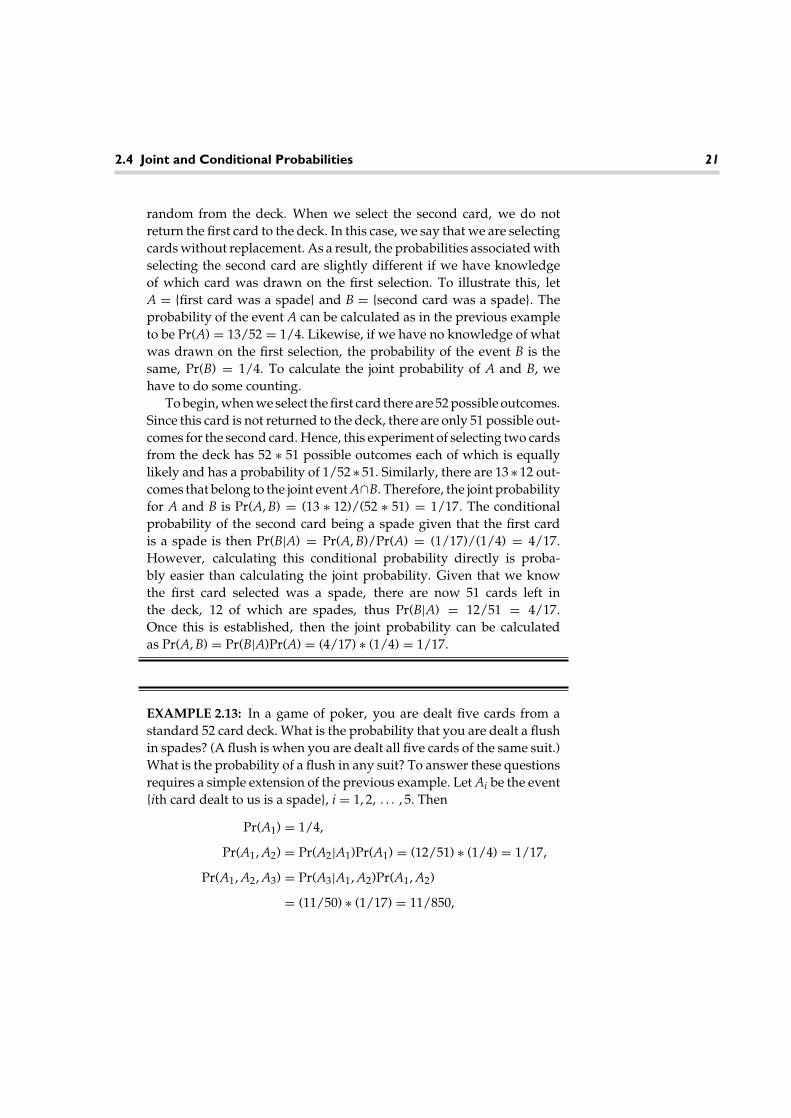
EXAMPLE 2.13: In a game of poker, you are dealt five cards from astandard 52 card deck. What is the probability that you are dealt a flushin spades? (A flush is when you are dealt all five cards of the same suit.)What is the probability of a flush in any suit? To answer these questionsrequires a simple extension of the previous example. Let Ai be the event{ith card dealt to us is a spade}, i = 1, 2, . . . , 5. Then
Pr(A1) = 1/4,
Pr(A1, A2) = Pr(A2|A1)Pr(A1) = (12/51) ∗ (1/4) = 1/17,
Pr(A1, A2, A3) = Pr(A3|A1, A2)Pr(A1, A2)
= (11/50) ∗ (1/17) = 11/850,

22 Chapter 2 Introduction to Probability Theory
Pr(A1, A2, A3, A4) = Pr(A4|A1, A2, A3)Pr(A1, A2, A3)
= (10/49) ∗ (11/850) = 11/4165,
Pr(A1, A2, A3, A4, A5) = Pr(A5|A1, A2, A3, A4)Pr(A1, A2, A3, A4)
= (9/48) ∗ (11/4165) = 33/66,640.
To find the probability of being dealt a flush in any suit, we proceed asfollows:
Pr(flush) = Pr({flush in spades} ∪ {flush in hearts}∪ {flush in diamonds} ∪ {flush in clubs})
= Pr(flush in spades) + Pr(flush in hearts)+ Pr(flush in diamonds) + Pr(flush in clubs).
Since all four events in the preceding expression have equal probability,then
Pr(flush) = 4 ∗ Pr(flush in spades) = 4 ∗ 3366,640
= 3316,660
.
2.5 Bayes’s Theorem
In this section, we develop a few results related to the concept of conditional prob-ability. While these results are fairly simple, they are so useful that we felt it wasappropriate to devote an entire section to them. To start with, the following theo-rem was essentially proved in the previous section and is a direct result of thedefinition of conditional probability.
THEOREM 2.4: For any events A and B such that Pr(B) �= 0,
Pr(A|B) = Pr(B|A)Pr(A)Pr(B)
. (2.12)
PROOF: From Definition 2.5,
Pr(A, B) = Pr(A|B)Pr(B) = Pr(B|A)Pr(A). (2.13)
Theorem 2.4 follows directly by dividing the preceding equations by Pr(B). �

2.5 Bayes’s Theorem 23
Theorem 2.4 is useful for calculating certain conditional probabilities since, inmany problems, it may be quite difficult to compute Pr(A|B) directly, whereascalculating Pr(B|A) may be straightforward.
THEOREM 2.5 (Theorem of Total Probability): Let B1, B2, . . . , Bn be a set ofmutually exclusive and exhaustive events. That is, Bi ∩ Bj = Ø for all i �= j and
n⋃i=1
Bi = S ⇒n∑
i=1
Pr(Bi) = 1. (2.14)
Then
Pr(A) =n∑
i=1
Pr(A|Bi)Pr(Bi) (2.15)
PROOF: As with Theorem 2.1, a Venn diagram (shown in Figure 2.2) is used hereto aid in the visualization of our result. From the diagram, it can be seen that theevent A can be written as
A = {A ∩ B1} ∪ {A ∩ B2} ∪ · · · ∪ {A ∩ Bn} (2.16)
⇒ Pr(A) = Pr({A ∩ B1} ∪ {A ∩ B2} ∪ · · · ∪ {A ∩ Bn}) (2.17)
Also, since the Bi are all mutually exclusive, then the {A ∩ Bi} are also mutuallyexclusive, so that
Pr(A) =n∑
i=1
Pr(A, Bi) (by Corollary 2.3), (2.18)
=n∑
i=1
Pr(A|Bi)Pr(Bi) (by Theorem 2.4). (2.19)
B5
A
B1
B2
B4
B3
S
Figure 2.2 Venn diagram used to help prove the theorem of total probability.

24 Chapter 2 Introduction to Probability Theory
Finally, by combining the results of Theorems 2.4 and 2.5, we get what has cometo be known as Bayes’s theorem. �
THEOREM 2.6 (Bayes’s Theorem): Let B1, B2, . . . , Bn be a set of mutually exclu-sive and exhaustive events. Then
Pr(Bi|A) = Pr(A|Bi)Pr(Bi)n∑
i=1Pr(A|Bi)Pr(Bi)
. (2.20)
As a matter of nomenclature, Pr(Bi) is often referred to as the a priori1 probability ofevent Bi, while Pr(Bi|A) is known as the a posteriori2 probability of event Bi given A.Section 2.8 presents an engineering application showing how Bayes’s theorem isused in the field of signal detection. We conclude here with a practical exampleshowing how useful Bayes’s theorem can be.
EXAMPLE 2.14: A certain auditorium has 30 rows of seats. Row 1 has11 seats, while Row 2 has 12 seats, Row 3 has 13 seats, and so on to theback of the auditorium where Row 30 has 40 seats. A door prize is tobe given away by randomly selecting a row (with equal probability ofselecting any of the 30 rows) and then randomly selecting a seat withinthat row (with each seat in the row equally likely to be selected). Findthe probability that Seat 15 was selected given that Row 20 was selectedand also find the probability that Row 20 was selected given that Seat 15was selected. The first task is straightforward. Given that Row 20 wasselected, there are 30 possible seats in Row 20 that are equally likelyto be selected. Hence, Pr(Seat 15|Row 20) = 1/30. Without the helpof Bayes’s theorem, finding the probability that Row 20 was selectedgiven that we know Seat 15 was selected would seem to be a formidableproblem. Using Bayes’s theorem,
Pr(Row 20|Seat 15) = Pr(Seat 15|Row20)Pr(Row 20)/Pr(Seat 15).
1The term a priori is Latin and is literally translated “from the former.” In this context, itrefers to probabilities that are formed from self-evident or presupposed models.
2The term a posteriori is also Latin and is literally translated “from the latter.” In thiscontext, it refers to probabilities that are derived or calculated after observing certainevents.

2.6 Independence 25
The two terms in the numerator on the right-hand side are both equalto 1/30. The term in the denominator is calculated using the help of thetheorem of total probability.
Pr(Seat 15) =30∑
k=5
1k + 10
130
= 0. 0342.
With this calculation completed, the a posteriori probability of Row 20being selected given seat 15 was selected is given by
Pr(Row 20|Seat 15) =1
301
300. 0342
= 0. 0325.
Note that the a priori probability that Row 20 was selected is 1/30 =0. 0333. Therefore, the additional information that Seat 15 was selectedmakes the event that Row 20 was selected slightly less likely. In somesense, this may be counterintuitive, since we know that if Seat 15 wasselected, there are certain rows that could not have been selected (i.e.,Rows 1–4 have fewer than 15 seats) and, therefore, we might expectRow 20 to have a slightly higher probability of being selected comparedto when we have no information about which seat was selected. To seewhy the probability actually goes down, try computing the probabilitythat Row 5 was selected given that Seat 15 was selected. The event thatSeat 15 was selected makes some rows much more probable, while itmakes others less probable and a few rows now impossible.
2.6 Independence
In Example 2.14, it was seen that observing one event can change the probabilityof the occurrence of another event. In that particular case, the fact that it wasknown that Seat 15 was selected, lowered the probability that Row 20 was selected.We say that the event A = {Row 20 was selected} is statistically dependent onthe event B = {Seat 15 was selected}. If the description of the auditorium werechanged so that each row had an equal number of seats (e.g., say all 30 rows had20 seats each), then observing the event B = {Seat 15 was selected} would notgive us any new information about the likelihood of the event A = {Row 20 wasselected}. In that case, we say that the events A and B are statistically independent.

26 Chapter 2 Introduction to Probability Theory
Mathematically, two events A and B are independent if Pr(A|B) = Pr(A). That is,the a priori probability of event A is identical to the a posteriori probability of Agiven B. Note that if Pr(A|B) = Pr(A), then the following two conditions also hold(see Exercise 2.8):
Pr(B|A) = Pr(B) (2.21)
Pr(A, B) = Pr(A)Pr(B). (2.22)
Furthermore, if Pr(A|B) �= Pr(A), then the other two conditions also do not hold.We can thereby conclude that any of these three conditions can be used as atest for independence and the other two forms must follow. We use the lastform as a definition of independence since it is symmetric relative to the eventsA and B.
DEFINITION 2.6: Two events are statistically independent if and only if
Pr(A, B) = Pr(A)Pr(B). (2.23)
EXAMPLE 2.15: Consider the experiment of tossing two numbereddice and observing the numbers that appear on the two upper faces.For convenience, let the dice be distinguished by color, with the firstdie tossed being red and the second being white. Let A = {number onthe red die is less than or equal to 2}, B = {number on the white die isgreater than or equal to 4}, and C = {the sum of the numbers on thetwo dice is 3}. As mentioned in the preceding text, there are severalways to establish independence (or lack thereof) of a pair of events. Onepossible way is to compare Pr(A, B) with Pr(A)Pr(B). Note that for theevents defined here, Pr(A) = 1/3, Pr(B) = 1/2, Pr(C) = 1/18. Also, ofthe 36 possible atomic outcomes of the experiment, six belong to theevent A ∩ B and hence Pr(A, B) = 1/6. Since Pr(A)Pr(B) = 1/6 as well,we conclude that the events A and B are independent. This agrees withintuition since we would not expect the outcome of the roll of one dieto affect the outcome of the other. What about the events A and C?Of the 36 possible atomic outcomes of the experiment, two belong tothe event A ∩ C and hence Pr(A, C) = 1/18. Since Pr(A)Pr(C) = 1/54,the events A and C are not independent. Again, this is intuitive sincewhenever the event C occurs, the event A must also occur and sothe two must be dependent. Finally, we look at the pair of events Band C. Clearly, B and C are mutually exclusive. If the white die showsa number greater than or equal to 4, there is no way the sum can be 3.

2.6 Independence 27
Hence, Pr(B, C) = 0 and since Pr(B)Pr(C) = 1/36, these two events arealso dependent.
The previous example brings out a point that is worth repeating. It is a commonmistake to equate mutual exclusiveness with independence. Mutually exclusiveevents are not the same thing as independent events. In fact, for two events A andB for which Pr(A) �= 0 and Pr(B) �= 0, A and B can never be both independent andmutually exclusive. Thus, mutually exclusive events are necessarily statisticallydependent.
A few generalizations of this basic idea of independence are in order. First, whatdoes it mean for a set of three events to be independent? The following definitionclarifies this and then we generalize the definition to any number of events.
DEFINITION 2.7: The events A, B, and C are mutually independent if each pairof events is independent; that is,
Pr(A, B) = Pr(A)Pr(B), (2.24a)
Pr(A, C) = Pr(A)Pr(C), (2.24b)
Pr(B, C) = Pr(B)Pr(C), (2.24c)
and in addition,
Pr(A, B, C) = Pr(A)Pr(B)Pr(C). (2.24d)
DEFINITION 2.8: The events A1, A2, . . . , An are independent if any subset of k <
n of these events are independent, and in addition
Pr(A1, A2, . . . , An) = Pr(A1)Pr(A2) . . . Pr(An). (2.25)
There are basically two ways in which we can use this idea of independence. Asshown in Example 2.15, we can compute joint or conditional probabilities and applyone of the definitions as a test for independence. Alternatively, we can assume inde-pendence and use the definitions to compute joint or conditional probabilities thatotherwise may be difficult to find. This latter approach is used extensively in engi-neering applications. For example, certain types of noise signals can be modeledin this way. Suppose we have some time waveform X(t) which represents a noisysignal that we wish to sample at various points in time, t1, t2, . . . , tn. Perhaps weare interested in the probabilities that these samples might exceed some threshold,so we define the events Ai = Pr(X(ti) > T), i = 1, 2, . . . , n. How might we calcu-late the joint probability Pr(A1, A2, . . . , An)? In some cases, we have every reason tobelieve that the value of the noise at one point in time does not affect the value of the

28 Chapter 2 Introduction to Probability Theory
noise at another point in time. Hence, we assume that these events are independentand write Pr(A1, A2, . . . , An) = Pr(A1)Pr(A2) . . . Pr(An).
2.7 Discrete Random Variables
Suppose we conduct an experiment, E, which has some sample space, S. Further-more, let ξ be some outcome defined on the sample space, S. It is useful to definefunctions of the outcome ξ , X = f (ξ ). That is, the function f has as its domain allpossible outcomes associated with the experiment, E. The range of the function fwill depend upon how it maps outcomes to numerical values but in general willbe the set of real numbers or some part of the set of real numbers. Formally, wehave the following definition.
DEFINITION 2.9: A random variable is a real-valued function of the elementsof a sample space, S. Given an experiment, E, with sample space, S, the randomvariable X maps each possible outcome, ξ ∈ S, to a real number X(ξ ) as specified bysome rule. If the mapping X(ξ ) is such that the random variable X takes on a finiteor countably infinite number of values, then we refer to X as a discrete randomvariable; whereas, if the range of X(ξ ) is an uncountably infinite number of points,we refer to X as a continuous random variable.
Since X = f (ξ ) is a random variable whose numerical value depends on theoutcome of an experiment, we cannot describe the random variable by stating itsvalue; rather, we must give it a probabilistic description by stating the probabilitiesthat the variable X takes on a specific value or values (e.g., Pr(X = 3) or Pr(X > 8)).For now, we will focus on random variables that take on discrete values and willdescribe these random variables in terms of probabilities of the form Pr(X = x).In the next chapter when we study continuous random variables, we will find thisdescription to be insufficient and will introduce other probabilistic descriptionsas well.
DEFINITION 2.10: The probability mass function (PMF), PX(x), of a random vari-able, X, is a function that assigns a probability to each possible value of the randomvariable, X. The probability that the random variable X takes on the specific valuex is the value of the probability mass function for x. That is, PX(x) = Pr(X = x).We use the convention that upper case variables represent random variableswhile lower case variables represent fixed values that the random variable canassume.

2.7 Discrete Random Variables 29
EXAMPLE 2.16: A discrete random variable may be defined for therandom experiment of flipping a coin. The sample space of outcomes isS = {H, T}. We could define the random variable X to be X(H) = 0 andX(T) = 1. That is, the sample space H, T is mapped to the set {0, 1} bythe random variable X. Assuming a fair coin, the resulting probabilitymass function is PX(0) = 1/2 and PX(1) = 1/2. Note that the mappingis not unique and we could have just as easily mapped the sample spaceH, T to any other pair of real numbers (e.g., {1, 2}).
EXAMPLE 2.17: Suppose we repeat the experiment of flipping a faircoin n times and observe the sequence of heads and tails. A randomvariable, Y, could be defined to be the number of times tails occurs inn trials. It turns out that the probability mass function for this randomvariable is
PY(k) =(
nk
) (12
)n
, k = 0, 1, . . . , n.
The details of how this PMF is obtained will be deferred until later inthis section.
EXAMPLE 2.18: Again, let the experiment be the flipping of a coin, andthis time we will continue repeating the event until the first time a headsoccurs. The random variable Z will represent the number of times untilthe first occurrence of a heads. In this case, the random variable Z cantake on any positive integer value, 1 ≤ Z < ∞. The probability massfunction of the random variable Z can be worked out as follows:
Pr(Z = n) = Pr(n − 1 tails followed by one heads)
= (Pr(T))n−1Pr(H) =(
12
)n−1 (12
)= 2−n.
Hence,
PZ(n) = 2−n, n = 1, 2, 3, . . . .

30 Chapter 2 Introduction to Probability Theory
0 1 2 3 4 5 6 7 8 9 100
0.05
0.1
0.15
0.2
0.25
k
PX(k
)
Comparison of Estimated and True PMF for Example 2.19
Relative frequencyTrue PMF
Figure 2.3 MATLAB simulation results from Example 2.19.
EXAMPLE 2.19: In this example, we will estimate the PMFgiven in Example 2.17 via MATLAB simulation using the relativefrequency approach. Suppose the experiment consists of tossingthe coin n = 10 times and counting the number of tails. We then
repeat this experiment a large number of times and count the relative fre-quency of each number of tails to estimate the PMF. The following MATLABcode can be used to accomplish this. Results of running this code are shownin Figure 2.3.
% Simulation code to estimate PMF of Example 2.17.
n=10; % Number of coin flips per
experiment.
m=100; % Number of times to repeat
experiment.
X=round(rand(n,m)); % Simulate coin flipping.
Y=sum(X); % Calculate number of tails per
experiment.
Rel_Freq=hist(Y,[0:n])/m; % Compute relative frequencies.
for k=0:n % Compute actual PMF.
PMF(k+1)=nchoosek(n,k)*(2∧(-n));end
% Plot Results

2.7 Discrete Random Variables 31
plot([0:n],Rel_Freq,‘o’,[0:n],PMF,‘*’)
legend(‘Relative frequency’,‘True PMF’)
xlabel(‘k’)
ylabel(‘P_X(k)’)
title(‘Comparison of Estimated and True PMF for Example 2.19’)
Try running this code using a larger value for m. You should see moreaccurate relative frequency estimates as you increase m.
From the preceding examples, it should be clear that the probability massfunction associated with a random variable, X, must obey certain properties. First,since PX(x) is a probability, it must be nonnegative and no greater than 1. Second,if we sum PX(x) over all x, then this is the same as the sum of the probabilities ofall outcomes in the sample space, which must be equal to 1. Stated mathematically,we may conclude that
0 ≤ PX(x) ≤ 1, (2.26a)∑x
PX(x) = 1. (2.26b)
When developing the probability mass function for a random variable, it is usefulto check that the PMF satisfies these properties.
In the paragraphs that follow, we describe some commonly used discrete ran-dom variables, along with their probability mass functions, and some real-worldapplications in which each might typically be used.
A. Bernoulli Random Variable This is the simplest possible random variable and isused to represent experiments that have two possible outcomes. These experimentsare called Bernoulli trials and the resulting random variable is called a Bernoulli ran-dom variable. It is most common to associate the values {0,1} with the two outcomesof the experiment. If X is a Bernoulli random variable, its probability mass functionis of the form
PX(0) = 1 − p, PX(1) = p. (2.27)
The coin tossing experiment would produce a Bernoulli random variable. In thatcase, we may map the outcome H to the value X = 1 and T to X = 0. Also, wewould use the value p = 1/2 assuming that the coin is fair. Examples of engineeringapplications might include radar systems where the random variable could indicatethe presence (X = 1) or absence (X = 0) of a target, or a digital communicationsystem where X = 1 might indicate a bit was transmitted in error while X = 0
32 Chapter 2 Introduction to Probability Theory
would indicate that the bit was received correctly. In these examples, we wouldprobably expect that the value of p would be much smaller than 1/2.
B. Binomial Random Variable Consider repeating a Bernoulli trial n times, wherethe outcome of each trial is independent of all others. The Bernoulli trial has asample space of S = {0, 1} and we say that the repeated experiment has a samplespace of Sn = {0, 1}n, which is referred to as a Cartesian space. That is, outcomes ofthe repeated trials are represented as n element vectors whose elements are takenfrom S. Consider, for example, the outcome
k times n − k times
ξk =︷ ︸︸ ︷(1, 1, . . . , 1,
︷ ︸︸ ︷0, 0, . . . , 0) .
(2.28)
The probability of this outcome occurring is
Pr(ξk) = Pr(1, 1, . . . , 1, 0, 0, . . . , 0) = Pr(1)Pr(1) . . . Pr(1)Pr(0)Pr(0) . . . Pr(0)
= (Pr(1))k(Pr(0))n−k = pk(1 − p)n−k. (2.29)
In fact, the order of the 1s and 0s in the sequence is irrelevant. Any outcome withexactly k 1s and n − k 0s would have the same probability. Now let the randomvariable X represent the number of times the outcome 1 occurred in the sequenceof n trials. This is known as a binomial random variable and takes on integer valuesfrom 0 to n. To find the probability mass function of the binomial random variable,let Ak be the set of all outcomes that have exactly k 1s and n − k 0s. Note that alloutcomes in this event occur with the same probability. Furthermore, all outcomesin this event are mutually exclusive. Then
PX(k) = Pr(Ak) = (# of outcomes in Ak) ∗ (probability of each outcome in Ak)
=(
nk
)pk(1 − p)n−k, k = 0, 1, 2, . . . , n. (2.30)
The number of outcomes in the event Ak is just the number of combinations ofn objects taken k at a time. This is the binomial coefficient, which is given by
(nk
)= n!
k!(n − k)! . (2.31)
As a check, we verify that this probability mass function is properly normalized:
n∑k=0
(nk
)pk(1 − p)n−k = (p + 1 − p)n = 1n = 1. (2.32)

2.7 Discrete Random Variables 33
In this calculation, we have used the binomial expansion
(a + b)n =n∑
k=0
(nk
)akbn−k. (2.33)
Binomial random variables occur in practice any time Bernoulli trials are repeated.For example, in a digital communication system, a packet of n bits may be transmit-ted and we might be interested in the number of bits in the packet that are receivedin error. Or, perhaps a bank manager might be interested in the number of tellerswho are serving customers at a given point in time. Similarly, a medical techni-cian might want to know how many cells from a blood sample are white and howmany are red. In Example 2.17, the coin tossing experiment was repeated n timesand the random variable Y represented the number of times heads occurred in thesequence of n tosses. This is a repetition of a Bernoulli trial, and hence the randomvariable Y should be a binomial random variable with p = 1/2 (assuming the coinis fair).
C. Poisson Random Variable Consider a binomial random variable, X, where thenumber of repeated trials, n, is very large. In that case, evaluating the binomialcoefficients can pose numerical problems. If the probability of success in eachindividual trial, p, is very small, then the binomial random variable can be wellapproximated by a Poisson random variable. That is, the Poisson random variable is alimiting case of the binomial random variable. Formally, let n approach infinity andp approach zero in such a way that limn→∞ np = α. Then the binomial probabilitymass function converges to the form
PX(m) = αm
m! e−α , m = 0, 1, 2, . . . , (2.34)
which is the probability mass function of a Poisson random variable. We see thatthe Poisson random variable is properly normalized by noting that
∞∑m=0
αm
m! e−α = e−αeα = 1. (2.35)
see Appendix E, (E.14).The Poisson random variable is extremely important as it describes the behavior
of many physical phenomena. It is most commonly used in queuing theory and incommunication networks. The number of customers arriving at a cashier in a storeduring some time interval may be well modeled as a Poisson random variable, asmay the number of data packets arriving at a given node in a computer network.We will see increasingly in later chapters that the Poisson random variable plays afundamental role in our development of a probabilistic description of noise.

34 Chapter 2 Introduction to Probability Theory
D. Geometric Random Variable Consider repeating a Bernoulli trial until the firstoccurrence of the outcome ξ0. If X represents the number of times the outcome ξ1occurs before the first occurrence of ξ0, then X is a geometric random variable whoseprobability mass function is
PX(k) = (1 − p)pk, k = 0, 1, 2, . . . . (2.36)
We might also formulate the geometric random variable in a slightly differentway. Suppose X counted the number of trials that were performed until thefirst occurrence of ξ0. Then the probability mass function would take on theform
PX(k) = (1 − p)pk−1, k = 1, 2, 3, . . . . (2.37)
The geometric random variable can also be generalized to the case where the out-come ξ0 must occur exactly m times. That is, the generalized geometric randomvariable counts the number of Bernoulli trials that must be repeated until the mthoccurrence of the outcome ξ0. We can derive the form of the probability mass func-tion for the generalized geometric random variable from what we know aboutbinomial random variables. For the mth occurrence of ξ0 to occur on the kth trial,then the first k−1 trials must have had m−1 occurrences of ξ0 and k−m occurrencesof ξ1. Then
PX(k) = Pr({((m − 1) occurrences of ξ0 in k − 1) trials}∩ {ξ0 occurs on the kth trial})
=(
k − 1m − 1
)pk−m(1 − p)m−1(1 − p)
=(
k − 1m − 1
)pk−m(1 − p)m, k = m, m + 1, m + 2, . . . . (2.38)
This generalized geometric random variable sometimes goes by the name of aPascal random variable or the negative binomial random variable.
Of course, one can define many other random variables and develop the asso-ciated probability mass functions. We have chosen to introduce some of the moreimportant discrete random variables here. In the next chapter, we will introducesome continuous random variables and the appropriate probabilistic descriptionsof these random variables. However, to close out this chapter, we provide a sec-tion showing how some of the material covered herein can be used in at least oneengineering application.

2.8 Engineering Application: An Optical Communication System 35
2.8 Engineering Application: An OpticalCommunication System
Figure 2.4 shows a simplified block diagram of an optical communication system.Binary data is transmitted by pulsing a laser or a light emitting diode (LED) thatis coupled to an optical fiber. To transmit a binary 1 we turn on the light sourcefor T seconds, while a binary 0 is represented by turning the source off for thesame time period. Hence, the signal transmitted down the optical fiber is a seriesof pulses (or absence of pulses) of duration T seconds that represents the string ofbinary data to be transmitted. The receiver must convert this optical signal back intoa string of binary numbers; it does this using a photodetector. The received lightwave strikes a photoemissive surface, which emits electrons in a random manner.While the number of electrons emitted during a T second interval is random andthus needs to be described by a random variable, the probability mass function ofthat random variable changes according to the intensity of the light incident on thephotoemissive surface during the T second interval. Therefore, we define a randomvariable X to be the number of electrons counted during a T second interval, andwe describe this random variable in terms of two conditional probability massfunctions PX|0(k) = Pr(X = k|0 sent) and PX|1(k) = Pr(X = k|1 sent). It can beshown through a quantum mechanical argument that these two probability massfunctions should be those of Poisson random variables. When a binary 0 is sent, arelatively low number of electrons is typically observed; whereas, when a 1 is sent,a higher number of electrons is typically counted. In particular, suppose the twoprobability mass functions are given by
PX|0(k) = Rk0
k! e−R0 , k = 0, 1, 2, . . . , (2.39a)
PX|1(k) = Rk1
k! e−R1 , k = 0, 1, 2, . . . . (2.39b)
In these two PMFs, the parameters R0 and R1 are interpreted as the “average”number of electrons observed when a 0 is sent and when a 1 is sent, respectively.
Laseror
LED
Photodetector (electroncounter)
DecisionDatainput{0,1}
{0,1}
Figure 2.4 Block diagram of an optical communication system.

36 Chapter 2 Introduction to Probability Theory
Also, it is assumed that R0 < R1, so when a 0 is sent we tend to observe fewerelectrons than when a 1 is sent.
At the receiver, we count the number of electrons emitted during each T secondinterval and then must decide whether a 0 or 1 was sent during each interval.Suppose that during a certain bit interval, it is observed that k electrons are emitted.A logical decision rule would be to calculate Pr(0 sent|X = k) and Pr(1 sent|X = k)and choose according to whichever is larger. That is, we calculate the a posterioriprobabilities of each bit being sent given the observation of the number of electronsemitted and choose the data bit that maximizes the a posteriori probability. This isreferred to as a maximum a posteriori (MAP) decision rule, and we decide that abinary 1 was sent if
Pr(1 sent|X = k) > Pr(0 sent|X = k); (2.40)
otherwise we decide a 0 was sent. Note that these desired a posteriori probabilitiesare backwards relative to how the photodetector was statistically described. Thatis, we know the probabilities of the form Pr(X = k|1 sent) but we want to knowPr(1 sent|X = k). We call upon Bayes’s theorem to help us convert what we knowinto what we desire to know. Using the theorem of total probability,
PX(k) = Pr(X = k) = PX|0(k)Pr(0 sent) + PX|1(k)Pr(1 sent). (2.41)
The a priori probabilities Pr(0 sent) and Pr(1 sent) are taken to be equal (to 1/2),so that
PX(k) = 12
Rk0
k! e−R0 + 12
Rk1
k! e−R1 . (2.42)
Therefore, applying Bayes’s theorem,
Pr(0 sent|X = k) = PX|0(k)Pr(0 sent)PX(k)
=12
Rk0
k! e−R0
12
Rk0
k! e−R0 + 12
Rk1
k! e−R1
, (2.43)
and
Pr(1 sent|X = k) = PX|1(k)Pr(1 sent)PX(k)
=12
Rk1
k! e−R1
12
Rk0
k! e−R0 + 12
Rk1
k! e−R1
, (2.44)
Since the denominators of both a posteriori probabilities are the same, we decidethat a 1 was sent if
12
Rk1
k! e−R1 >12
Rk0
k! e−R0 . (2.45)

2.8 Engineering Application: An Optical Communication System 37
After a little algebraic manipulation, this reduces down to choosing in favorof a 1 if
k >R1 − R0
ln(R1/R0); (2.46)
otherwise, we choose in favor of 0. That is, the receiver for our optical communi-cation system counts the number of electrons emitted and compares that numberwith a threshold. If the number of electrons emitted is above the threshold wedecide that a 1 was sent; otherwise, we decide a 0 was sent.
We might also be interested in evaluating how often our receiver makes a wrongdecision. Ideally, the answer is that errors are rare, but still we would like toquantify this. Toward that end, we note that errors can occur in two manners.First a 0 could be sent and the number of electrons observed could fall above thethreshold, causing us to decide that a 1 was sent. Likewise, if a 1 is actually sentand the number of electrons observed is low, we would mistakenly decide that a 0was sent. Again, invoking concepts of conditional probability, we see that
Pr(error) = Pr(error|0 sent)Pr(0 sent) + Pr(error|1 sent)Pr(1 sent). (2.47)
Let x0 be the threshold with which we compare X to decide which data bit wassent. Specifically, let x0 = (R1 − R0)/ln(R1/R0)� so that we decide a 1 was sent ifX > x0, and we decide a 0 was sent if X ≤ x0. Then
Pr(error|0 sent) = Pr(X > x0|0 sent) =∞∑
k=x0+1
PX|0(k)
=∞∑
k=x0+1
Rk0
k! e−R0 = 1 −x0∑
k=0
Rk0
k! e−R0 . (2.48)
Likewise,
Pr(error|1 sent) =x0∑
k=0
PX|0(k) =x0∑
k=0
Rk1
k! e−R1 . (2.49)
Hence, the probability of error for our optical communication system is
Pr(error) = 12
− 12
x0∑k=0
Rk0e−R0 − Rk
1e−R1
k! . (2.50)
Figure 2.5 shows a plot of the probability of error as a function of R1 with R0 as aparameter. The parameter R0 is a characteristic of the photodetector used. We willsee in later chapters that R0 can be interpreted as the “average” number of electrons

38 Chapter 2 Introduction to Probability Theory
0 5 10 15 20 25 30 35 4010−8
10−6
10−4
10−2
100P
roba
bilit
y of
err
or
R0 = 1
R0 = 2
R0 = 4
R0 = 7
R0 = 10
R1
Figure 2.5 Probability of error curves for an optical communication system; curves areparameterized from bottom to top with R0 = 1, 2, 4, 7, 10.
emitted during a bit interval when there is no signal incident of the photodetector.This is sometimes referred to as the “dark current.” The parameter R1 is controlledby the intensity of the incident light. Given a certain photodetector, the value ofthe parameter R0 can be measured. The value of R1 required to achieve a desiredprobability of error can be found from Figure 2.5 (or from Equation 2.50, whichgenerated the figure). The intensity of the laser or LED can then be adjusted toproduce the required value for the parameter R1.
Exercises2.1 Using mathematical induction, prove Corollary 2.1. Recall that
Corollary 2.1 states that for M events A1, A2, . . . , AM that are mutuallyexclusive (i.e., Ai ∩ Aj = Ø for all i �= j),
Pr
( M⋃i=1
Ai
)=
M∑i=1
Pr(Ai).
2.2 Develop a careful proof of Theorem 2.1, which states that for any events Aand B,
Pr(A ∪ B) = Pr(A) + Pr(B) − Pr(A ∩ B).

Exercises 39
One way to approach this proof is to start by showing that the set A ∪ Bcan be written as the union of three mutually exclusive sets,
A ∪ B = {A ∩ (A ∩ B)} ∪ {A ∩ B} ∪ {B ∩ (A ∩ B)}and hence by Corollary 2.1,
Pr(A ∪ B) = Pr(A ∩ (A ∩ B)) + Pr(A ∩ B) + Pr(B ∩ (A ∩ B)).
Next, show that
Pr(A ∩ (A ∩ B)) = Pr(A) − Pr(A ∩ B)
and likewise
Pr(B ∩ (A ∩ B)) = Pr(B) − Pr(A ∩ B).
(Hint: Recall DeMorgan’s law) Put these results together to complete thedesired proof.
2.3 Show that the above formula for the probability of the union of two eventscan be generalized to three events as follows:
Pr(A ∪ B ∪ C) = Pr(A) + Pr(B) + Pr(C)
− Pr(A ∩ B) − Pr(A ∩ C) − Pr(B ∩ C) + Pr(A ∩ B ∩ C).
2.4 Prove Theorem 2.3, which states that if A ⊂ B then Pr(A) ≤ Pr(B).
2.5 Formally prove the union bound which states that for any eventsA1, A2, . . . , AM (not necessarily mutually exclusive),
Pr
( M⋃i=1
Ai
)≤
M∑i=1
Pr(Ai).
2.6 (a) Demonstrate that the relative frequency approach to assigning proba-bilities satisfies the three axioms of probability.
(b) Demonstrate that the definition of conditional probability Pr(A|B) =Pr(A, B)/Pr(B) satisfies the three axioms of probability.
2.7 Prove that if Pr(B|A) = Pr(B), then it follows that
(a) Pr(A, B) = Pr(A)Pr(B), and(b) Pr(A|B) = Pr(A).

40 Chapter 2 Introduction to Probability Theory
Furthermore, show that if Pr(B|A) �= Pr(B), then the two conditions (a) and(b) do not hold as well.
2.8 We are given a number of darts. When we throw a dart at a target, we have aprobability of 1/4 of hitting the target. What is the probability of obtainingat least one hit if three darts are thrown? Calculate this probability twoways. Hint: Construct the sample space. How many outcomes are in thesample space? Are all outcomes in the sample space equally likely?
2.9 A box of 30 diodes is known to contain five defective ones. If two diodesare selected at random without replacement, what is the probability thatat least one of these diodes is defective?
2.10 Two balls are selected sequentially (without replacement) from an urncontaining three red, four white, and five blue balls.
(a) What is the probability that the first is red and the second is blue?
(b) What is the probability of selecting a white ball on the second draw ifthe first ball is replaced before the second is selected?
(c) What is the probability of selecting a white ball on the second draw ifthe first ball is not replaced before the second is selected?
2.11 In pulse code modulation (PCM), a PCM word consists of a sequence ofbinary digits (bits) of 1s and 0s.
(a) Suppose the PCM word length is n bits long. How many distinct wordsare there?
(b) If each PCM word, three bits long, is equally likely to occur, what is theprobability of a word with exactly two 1s occurring? Solve this prob-lem in two ways. First, consider all words in a sample space. Second,suppose each bit is equally likely.
2.12 In pulse amplitude modulation (PAM), a PAM word consists of a sequenceof pulses, where each pulse may take on a given number of amplitudelevels. Suppose a PAM word is n pulses long and each pulse may take onm different levels.
(a) How many distinct PAM words are there?
(b) If each PAM word, four pulses long, is equally likely to occur and eachpulse can have one of three levels, {0, 1, 2}, what is the probability of aPAM word occurring with exactly two pulses of level 2?

Exercises 41
2.13 A balanced coin is tossed nine times. Find the probabilities of each of thefollowing events:
(a) exactly 3 heads occurred;
(b) at least 3 heads occurred;
(c) at least 3 heads and at least 2 tails occurred.
2.14 Two six-sided (balanced) dice are thrown. Find the probabilities of each ofthe following events:
(a) a 5 does not occur on either throw;
(b) the sum is 7;
(c) a 5 and a 3 occur in any order;
(d) the first throw is a 5 and the second throw is a 5 or a 4;
(e) both throws are 5;
(f) either throw is a 6.
2.15 Two six-sided (balanced) dice are thrown. Find the probabilities of each ofthe following events:
(a) only 2, 3, or 4 appear on both dice;
(b) the value of the second roll subtracted from the value of the first roll is 2;
(c) the sum is 10 given that one roll is 6;
(d) the sum is 7 or 8 given that one roll is 5;
(e) one roll is a 4 given that the sum is 7.
2.16 Manufacturer X produces personal computers (PCs) at two different loca-tions in the world. Fifteen percent of the PCs produced at location A aredelivered defective to a retail outlet, while 5 percent of the PCs produced atlocation B are delivered defective to the same retail store. If the manufactur-ing plant at A produces 1,000,000 PCs per year and the plant at B produces150,000 PCs per year, find the probability of purchasing a defective PC.
2.17 I deal myself 3 cards for a standard 52-card deck. Find the probabilities ofeach of the following events:
(a) 2 of a kind (e.g., 2 fives or 2 kings),
(b) 3 of a kind,
(c) 3 of the same suit (a.k.a. a flush, e.g., 3 hearts or 3 clubs),
(d) 3 cards in consecutive order (a.k.a. a straight, e.g., 2-3-4 or 10-J-Q).

42 Chapter 2 Introduction to Probability Theory
2.18 I deal myself 5 cards for a standard 52-card deck. Find the probabilities ofeach of the following events:
(a) 2 of a kind,(b) 3 of a kind,(c) 2 pair (e.g., 2 eights and 2 queens),(d) a flush (5 cards all of the same suit),(e) a full house (3 of one kind and 2 of another kind),(f) a straight (5 cards in consecutive order).
2.19 I deal myself 13 cards for a standard 52-card deck. Find the probabilitiesof each of the following events:
(a) exactly one heart appears in my hand (of 13 cards);(b) at least 7 cards from a single suit appear in my hand;(c) my hand is void (0 cards) of at least one suit.
2.20 Cards are drawn from a standard 52-card deck until an ace is drawn. Aftereach card is drawn, (if the card is not an ace), it is put back in the deckand the cards are reshuffled so that each card drawn is independent of allothers.
(a) Find the probability that the first ace is drawn on the 5th selection.(b) Find the probability that at least 5 cards are drawn before the first ace
appears.(c) Repeat parts (a) and (b) if the cards are drawn without replacement.
That is, after each card is drawn, (if it is not an ace) the card is set asideand not replaced in the deck.
2.21 Cards are drawn from a standard 52-card deck until the third club is drawn.After each card is drawn, it is put back in the deck and the cards arereshuffled so that each card drawn is independent of all others.
(a) Find the probability that the 3rd club is drawn on the 8th selection.(b) Find the probability that at least 8 cards are drawn before the 3rd club
appears.(c) Repeat parts (a) and (b) if the cards are drawn without replacement.
That is, after each card is drawn, the card is set aside and not replacedin the deck.
2.22 A computer memory has the capability of storing 106 words. Due to out-side forces, portions of the memory are often erased. Therefore, words are

Exercises 43
stored redundantly in various areas of the memory. If a particular wordis stored in n different places in the memory, what is the probability thatthis word cannot be recalled if one-half of the memory is erased by electro-magnetic radiation? Hint: Consider each word to be stored in a particularcell (or box). These cells (boxes) may be located anywhere, geometricallyspeaking, in memory. The contents of each cell may be either erased or noterased. Assume n is small compared to the memory capacity.
2.23 If two events A and B can occur and Pr(A) is not zero and Pr(B) is not zero,what combinations of independent (I), not independent (NI), mutuallyexclusive (M), and not mutually exclusive (NM) are permissible? In otherwords, which of the four combinations (I, M), (NI, M), (I, NM), and (NI,NM) are permissible? Construct an example for those combinations thatare permissible.
2.24 A possible outcome of an experiment is the event A. The probability of thisevent is p. The experiment is performed n times, and the outcome of anytrial is not affected by the results of the previous trials. Define a randomvariable X to be the number of times the event A occurs in n trials.
(a) What is the PMF Pr(X = x)?
(b) Show that the sum of the PMF over all x is 1.
(c) What is the name of this PMF?
2.25 For each of the following probability mass functions, find the value of theconstant c.
(a) PX(k) = c(0. 37)k, k = 0, 1, 2, . . .
(b) PX(k) = c(0. 82)k, k = 0, 1, 2, 3, . . .
(c) PX(k) = c(0. 41)k, k = 0, 1, 2, . . . , 24
(d) PX(k) = c(0. 91)k, k = 0, 1, 2, 3, . . . , 15
(e) PX(k) = c(0. 41)k, k = 0, 2, 4, . . . , 12
2.26 Consider a Bernoulli trial where Pr(1) = p and Pr(0) = 1 − p. Suppose thisBernoulli trial is repeated n times.
(a) Plot the probability mass function for a binomial random variable, X,with p = 1/5 and n = 10.
(b) Plot the corresponding probability mass function for a Poisson randomvariable X with α = np = 2.

44 Chapter 2 Introduction to Probability Theory
(c) Compare Pr(X ≥ 5) as computed by both the binomial and Poissonrandom variables. Is the Poisson random variable a good approxima-tion for the binomial random variable for this example?
2.27 Suppose the arrival of telephone calls at a switch can be modeled with aPoisson PMF. That is, if X is the number of calls that arrives in t minutes,then
Pr(X = k) = (λt)k
k! e−λt, k = 0, 1, 2, . . . ,
where λ is the average arrival rate in calls/minute. Suppose that theaverage rate of calls is 10 per minute.
(a) What is the probability that fewer than three calls will be received inthe first 6 seconds?
(b) What is the probability that fewer than three calls will be received inthe first 6 minutes?
2.28 In a certain lottery, six numbers are randomly chosen from the set{0, 1, 2, . . . , 49} (without replacement). To win the lottery, a player mustguess correctly all six numbers, but it is not necessary to specify in whichorder the numbers are selected.
(a) What is the probability of winning the lottery with only one ticket?
(b) Suppose in a given week, 6 million lottery tickets are sold. Supposefurther that each player is equally likely to choose any of the possiblenumber combinations and does so independently of the selections of allother players. What is the probability that exactly four players correctlyselect the winning combination?
(c) Again assuming 6 million tickets sold, what is the most probablenumber of winning tickets?
(d) Repeat parts (b) and (c) using the Poisson approximation to the bino-mial probability distribution. Is the Poisson distribution an accurateapproximation in this example?
2.29 Imagine an audio amplifier contains six transistors. Harry has determinedthat two transistors are defective, but he does not know which two. Harryremoves three transistors at random and inspects them. Let X be the num-ber of defective transistors that Harry finds, where X may be 0, 1, or 2.Find the PMF for X.

MATLAB Exercises 45
2.30 A software manufacturer knows that one out of 10 software games that thecompany markets will be a financial success. The manufacturer selects 10new games to market. What is the probability that exactly one game willbe a financial success? What is the probability that at least two games willbe a success?
2.31 Prove the following identities involving the binomial coefficient(
nk
)=
n!k!(n − k)! .
(a)(
nk
)=
(n
n − k
)
(b)(
nk
)+
(n
k + 1
)=
(n + 1k + 1
)
(c)n∑
k=0
(nk
)= 2n
(d)n∑
k=0
(nk
)(−1)k = 0
(e)n∑
k=1
(nk
)k = n2n−1
(f)n∑
k=0
(nk
)k(−1)k = 0
2.32 In a digital communication system, a block of k data bits is mapped intoan n bit codeword that typically contains the k information bits as well asn − k redundant bits. This is known as an (n, k) block code. The redundantbits are included to provide error correction capability. Suppose that eachtransmitted bit in our digital communication system is received in errorwith probability p. Furthermore, assume that the decoder is capable ofcorrecting any pattern of t or fewer errors in an n bit block. That is, if t orfewer bits in an n bit block are received in error, then the codeword willbe decoded correctly, whereas if more than t errors occur, the decoder willdecode the received word incorrectly. Assuming each bit is received inerror with probability p = 0. 03, find the probability of decoder error foreach of the following codes.
(a) (n, k) = (7, 4), t = 1(b) (n, k) = (15, 7), t = 2(c) (n, k) = (31, 16), t = 3
MATLAB Exercises2.33 Write the MATLAB code to produce a randomly generated number that
is equally likely to produce any number from the set {0, 1, 2, . . . , 9}.

46 Chapter 2 Introduction to Probability Theory
2.34 Write the MATLAB code to produce a randomly generated number thatfollows the Bernoulli distribution for an arbitrary parameter, p.
2.35 Modify the MATLAB code in Example 2.19 to produce a random variablethat follows a binomial distribution for arbitrary parameters n, p.
2.36 Write the MATLAB code to simulate a random variable, Z, whose PMF isgiven by Pz(k) = 2−k, k = 1, 2, 3, . . . . Hint: See Example 2.18 for specifics onhow this random variable arises and then follow the lead of Example 2.19.
2.37 (a) Write and execute a MATLAB program to calculate n! for an arbitrary n.Use your program to calculate 64!.
(b) What is the largest integer n for which your program gives a finiteanswer?
(c) Sterling’s approximation for the factorial function is given by
n! ≈ √2π
(nn+ 1
2
)e−n
(1 − 1
12n
).
Use your program to compare the true value of n! with Sterling’sapproximation. For what ranges of n is the approximation within1 percent of the true value?
2.38 Write your own program to evaluate the binomial coefficient(
nk
)=
n!k!(n − k)! . Create your program in such a way that it need not directly
evaluate n!. That way the program will not crash if you use it to evaluate abinomial coefficient n greater than the value you found in Exercise 2.37b.
Use your program to evaluate(
38415
).

Random Variables,Distributions, andDensity Functions 3
At the end of the last chapter, we introduced the concept of a random variableand gave several examples of common discrete random variables. These randomvariables were described by their probability mass functions. While this descrip-tion works fine for discrete random variables, it is inadequate to describe randomvariables that take on a continuum of values. We will illustrate through an exampleshortly. In this chapter, we introduce the cumulative distribution function as analternative description of random variables that is appropriate for describing con-tinuous as well as discrete random variables. A related function, the probabilitydensity function is also covered. With these tools in hand, the concepts of randomvariables can be fully developed. Several examples of commonly used continuousrandom variables are also discussed.
To show the need for an alternative to the probability mass function, considera discrete random variable, X, that takes on values from the set {0, 1/N, 2/N, . . . ,(N − 1)/N} with equal probability. That is, the probability mass function of X is
PX
(kN
)= 1
N, k = 0, 1, 2, . . . , N − 1. (3.1)
This is the type of random variable that is produced by “random” number gen-erators in high-level languages, such as Fortran and C, and in math packages suchas MATLAB, MathCAD, and Mathematica. In these cases, N is taken to be a fairlylarge number so that it appears that the random number can be anything in the con-tinuous range [0, 1). The reader is referred to Chapter 12, Simulation Techniques,for more details on how computer-generated random numbers work. For now,
47

48 Chapter 3 Random Variables, Distributions, and Density Functions
consider the limiting case as N → ∞ so that the random variable can truly fallanywhere in the interval [0,1). One curious result of passing to the limit is that now
PX
(kN
)= lim
N→∞1N
= 0. (3.2)
That is, each point has zero probability of occurring. Yet, something has to occur!This problem is common to continuous random variables, and it is clear that theprobability mass function is not a suitable description for such a random vari-able. The next sections develop two alternative descriptions for continuous randomvariables, which will be used extensively throughout the rest of the text.
3.1 The Cumulative Distribution Function
Since a continuous random variable will typically have a zero probability of takingon a specific value, we avoid talking about such probabilities. Instead, events ofthe form {X ≤ x} can be considered.
DEFINITION 3.1: The cumulative distribution function (CDF) of a random vari-able, X, is
FX(x) = Pr(X ≤ x). (3.3)
From this definition, several properties of the CDF can be inferred. First, sincethe CDF is a probability, it must take on values between 0 and 1. Since randomvariables are real-valued, it is easy to conclude that FX(−∞) = 0 and FX(∞) = 1.That is, a real number cannot be less than −∞ and must be less than ∞. Next, if weconsider two fixed values, x1 and x2, such that x1 < x2, then the event {X ≤ x1} is asubset of {X ≤ x2}. Hence, Fx(x1) ≤ Fx(x2). This implies that the CDF is a monotonicnondecreasing function. Also, we can break the event {X ≤ x2} into the union of twomutually exclusive events, {X ≤ x2} = {X ≤ x1} ∪ {x1 < X ≤ x2}. Hence, FX(x2) =FX(x1) + Pr(x1 < X ≤ x2) or, equivalently, Pr(x1 < X ≤ x2) = FX(x2) − FX(x1).Thus, the CDF can also be used to measure the probability that a random variabletakes on a value in a certain interval. These properties of cumulative distributionfunctions are summarized as follows:
(1) FX(−∞) = 0, FX(∞) = 1, (3.4a)
(2) 0 ≤ FX(x) ≤ 1, (3.4b)
3.1 The Cumulative Distribution Function 49
(3) For x1 < x2, FX(x1) ≤ FX(x2), (3.4c)
(4) For x1 < x2, Pr(x1 < X ≤ x2) = FX(x2) − FX(x1). (3.4d)
EXAMPLE 3.1: Which of the following mathematical functions couldbe the CDF of some random variable?
(a) FX(x) = 12
+ 1π
tan−1(x),
(b) FX(x) = [1 − e−x]u(x), (u(x) is the unit step function),
(c) FX(x) = e−x2,
(d) FX(x) = x2u(x).
To determine this, we need to check that the function starts at 0when x = −∞, ends at 1 when x = ∞, and is monotonic increasing inbetween. The first two functions satisfy these properties and thus arevalid CDFs, while the last two do not. The function in (c) is decreasingfor positive values of x, while the function in (d) takes on values greaterthan 1 and FX(∞) �= 1.
To more carefully illustrate the behavior of the CDF, let us return to the com-puter random number generator that generates N possible values from the set{0, 1/N, 2/N, . . . , (N − 1)/N} with equal probability. The CDF for this particularrandom variable can be described as follows. First, FX(x) = 0 for all x < 0, sincethe random variable cannot take on negative values. Similarly, FX(x) = 1 for allx ≥ (N − 1)/N since the random variable cannot be greater than (N − 1)/N. Next,consider a value of x in the range 0 ≤ x < 1/N. In this case, Pr(X ≤ x) = Pr(X = 0)since the only value in the specified range that this random variable can take onis X = 0. Hence, FX(x) = Pr(X = 0) = 1/N for 0 ≤ x < 1/N. Similarly, for1/N ≤ x < 2/N, FX(x) = Pr(X = 0) + Pr(X = 1/2N) = 2/N.
Following this same reasoning, it is seen that, in general, for an integer k suchthat 0 < k < N and (k − 1)/N ≤ x < k/N, FX(x) = k/N. A plot of FX(x) as afunction of x would produce the general staircase type function shown in Figure 3.1.In Figures 3.2(a) and 3.2(b), the CDF is shown for specific values of N = 10 andN = 50, respectively. It should be clear from these plots that in the limit as N passesto infinity, the CDF of Figure 3.2(c) results. The functional form of this CDF is
FX(x) =
0 x ≤ 0x 0 < x ≤ 1.1 x > 1
(3.5)

50 Chapter 3 Random Variables, Distributions, and Density Functions
3/N
2/N1/N
1/N 2/N N−2N
------------ N−1N
. . .
1
FX(x)
x
------------
Figure 3.1 General CDF of the random variable X.
In this limiting case, the random variable X is a continuous random variable andtakes on values in the range [0, 1) with equal probability. Later in the chapter,this will be referred to as a uniform random variable. Note that when the randomvariable was discrete, the CDF was discontinuous and had jumps at the specificvalues that the random variable could take on; whereas, for the continuous ran-dom variable, the CDF was a continuous function (although its derivative was notalways continuous). This last observation turns out to be universal in that contin-uous random variables have a continuous CDF, while discrete random variableshave a discontinuous CDF with a staircase type of function. Occasionally, one alsoneeds to work with a random variable whose CDF is continuous in some rangesand yet also has some discontinuities. Such a random variable is referred to asa mixed random variable.
EXAMPLE 3.2: Suppose we are interested in observing the occurrenceof certain events and noting the time of first occurrence. The event mightbe the emission of a photon in our optical photo detector at the endof Chapter 2, the arrival of a message at a certain node in a computercommunications network, or perhaps the arrival of a customer in a store.Let X be a random variable that represents the time that the event firstoccurs. We would like to find the CDF of such a random variable, FX(t) =Pr(X ≤ t). Since the event could happen at any point in time and timeis continuous, we expect X to be a continuous random variable. Toformulate a reasonable CDF for this random variable, suppose we dividethe time interval (0, t] into many, tiny nonoverlapping time intervals of

3.1 The Cumulative Distribution Function 51
(a) (b)
0 0.2 0.4 0.6 0.8 1 1.2 1.4 1.6 1.8 20
0.2
0.4
0.6
0.8
1
x
Fx(
x)
Fx(
x)
Fx(
x)
CDF of the Random Variable X for N=10
0 0.2 0.4 0.6 0.8 1 1.2 1.4 1.6 1.8 20
0.2
0.4
0.6
0.8
1
x
(c)
x
CDF of the Random Variable X for N=50
0 0.2 0.4 0.6 0.8 1 1.2 1.4 1.6 1.8 20
0.2
0.4
0.6
0.8
1
CDF of the Random Variable X as N Goes to Infinity
Figure 3.2 CDF of the random variable X for (a) N = 10, (b) N = 50, and (c) N → ∞.
length �t. Assume that the probability that our event occurs in a timeinterval of length �t is proportional to �t and take λ to be the constantof proportionality. That is
Pr(event occurs in (k�t, (k + 1)�t)) = λ�t.
We also assume that the event occurring in one interval is independentof the event occurring in another nonoverlapping time interval. Withthese rather simple assumptions, we can develop the CDF of the random

52 Chapter 3 Random Variables, Distributions, and Density Functions
variable X as follows:
FX(t) = Pr(X ≤ t) = 1 − Pr(X > t),
Pr(X > t) = Pr(X /∈ (0, t]) = Pr({X /∈ (0, �t]} ∩ {X /∈ (�t, 2�t]}∩ · · · ∩ {X /∈ ((k − 1)�t, k�t]}).
In this equation, it is assumed that the time interval (0, t] has beendivided into k intervals of length �t. Since each of the events in theexpression are independent, the probability of the intersection is justthe product of the probabilities, so that
Pr(X > t) = Pr(X /∈ (0, �t]) Pr(X /∈ (�t, 2�t]) · · · Pr(X /∈ ((k − 1)�t, k�t])
= (1 − λ�t)k =(
1 − λtk
)k
.
Finally, we pass to the limit as �t → 0 or, equivalently, k → ∞ toproduce
Pr(X > t) = e−λtu(t) ⇒ FX(t) = (1 − e−λt) u(t).
EXAMPLE 3.3: Suppose a random variable has a CDF given by FX(x) =(1 − e−x)u(x). Find the following quantities:
(a) Pr(X > 5),
(b) Pr(X < 5),
(c) Pr(3 < X < 7),
(d) Pr(X > 5∣∣X < 7).
For part (a), we note that Pr(X > 5) = 1 − Pr(X ≤ 5) = 1 − FX(5) = e−5.In part (b), we note that FX(5) gives us Pr(X ≤ 5), which is not quitewhat we want. However, we note that
FX(5) = Pr({X < 5} ∪ {X = 5}) = Pr(X < 5) + Pr(X = 5).
Hence,
Pr(X < 5) = FX(5) − Pr(X = 5).
In this case, since X is a continuous random variable, Pr(X = 5) = 0and so there is no need to make a distinction between Pr(X < 5) and

3.2 The Probability Density Function 53
Pr(X ≤ 5); however, for discrete random variables we would need tobe careful. Accordingly, Pr(X < 5) = FX(5) = 1 − exp(−5). For part (c),we note that in general FX(7) − FX(3) = Pr(3 < X ≤ 7). Again, forthis continuous random variable, Pr(X = 7) = 0, so we can also writePr(3 < X < 7) = FX(7) − FX(3) = e−3 − e−7. Finally, for part (d) we invokethe definition of conditional probability to write the required quantityin terms of the CDF of X:
Pr(X > 5|X < 7) = Pr({X > 5} ∩ {X < 7})Pr(X < 7)
= Pr(5 < X < 7)Pr(X < 7)
= FX(7) − FX(5)FX(7)
= e−5 − e−7
1 − e−7 .
For discrete random variables, the CDF can be written in terms of the probabilitymass function defined in Chapter 2. Consider a general random variable, X, whichcan take on values from the discrete set {x1, x2, x3, . . . }. The CDF for this randomvariable is
FX(x) =k∑
i=1
PX(xi), for xk ≤ x < xk+1. (3.6)
The constraint in this equation can be incorporated using unit step functions, inwhich case the CDF of a discrete random variable can be written as
FX(x) =k∑
i=1
PX(xi) u(x − xi). (3.7)
In conclusion, if we know the PMF of a discrete random variable, we can easilyconstruct its CDF.
3.2 The Probability Density Function
While the CDF introduced in the last section represents a mathematical tool tostatistically describe a random variable, it is often quite cumbersome to workwith CDFs. For example, we will see later in this chapter that the most impor-tant and commonly used random variable, the Gaussian random variable, has aCDF that cannot be expressed in closed form. Furthermore, it can often be difficultto infer various properties of a random variable from its CDF. To help circumventthese problems, an alternative and often more convenient description known asthe probability density function (PDF) is often used.

54 Chapter 3 Random Variables, Distributions, and Density Functions
DEFINITION 3.2: The probability density function (PDF) of the random variableX evaluated at the point x is
fX(x) = limε→0
Pr(x ≤ X < x + ε)ε
. (3.8)
As the name implies, the probability density function is the probability that the ran-dom variable X lies in an infinitesimal interval about the point X = x, normalizedby the length of the interval.
Note that the probability of a random variable falling in an interval can bewritten in terms of its CDF as specified in Equation 3.4d. For continuous randomvariables,
Pr(x ≤ X < x + ε) = FX(x + ε) − FX(x) (3.9)
so that
fX(x) = limε→0
FX(x + ε) − FX(x)ε
= dFX(x)dx
. (3.10)
Hence, it is seen that the PDF of a random variable is the derivative of its CDF.Conversely, the CDF of a random variable can be expressed as the integral of itsPDF. This property is illustrated in Figure 3.3. From the definition of the PDF inEquation 3.8, it is apparent that the PDF is a nonnegative function, although it is notrestricted to be less than unity as with the CDF. From the properties of the CDFs,we can also infer several important properties of PDFs as well. Some properties ofPDFs are
(1) fX(x) ≥ 0; (3.11a)
(2) fX(x) = dFX(x)dx
; (3.11b)
(3) FX(x) =∫ x
−∞fX(y) dy; (3.11c)
x
FX(xo) = area
fX(x)
xo
Figure 3.3 Relationship between the PDF and CDF of a random variable.

3.2 The Probability Density Function 55
(4)∫ ∞
−∞fX(x) dx = 1; (3.11d)
(5)∫ b
afX(x) dx = Pr(a < X ≤ b).
(3.11e)
EXAMPLE 3.4: Which of the following are valid probability densityfunctions?
(a) fX(x) = e−xu(x);
(b) fX(x) = e−|x|;
(c) fX(x) ={
34 (x2 − 1) |x| < 20 otherwise
;
(d) fX(x) ={
1 0 ≤ x < 10 otherwise
;
(e) fX(x) = 2xe−x2u(x).
To verify the validity of a potential PDF, we need to verify only thatthe function is nonnegative and normalized so that the area underneaththe function is equal to unity. The function in part (c) takes on negativevalues while the function in part (b) is not properly normalized, andhence these are not valid PDFs. The other three functions are valid PDFs.
EXAMPLE 3.5: A random variable has a CDF given by FX(x) =(1 − e−λx) u(x). Its PDF is then given by
fX(x) = dFX(x)dx
= λe−λxu(x).
Likewise, if a random variable has a PDF given by fX(x) = 2xe−x2u(x),
then its CDF is given by
FX(x) =∫ x
−∞fX(y) dy =
∫ x
−∞2ye−y2
u(y) dy
=∫ x
02ye−y2
dyu(x) = (1 − e−x2)u(x).

56 Chapter 3 Random Variables, Distributions, and Density Functions
EXAMPLE 3.6: The MATLAB function rand generates randomnumbers that are uniformly distributed in the interval (0,1) usingan algorithm to be discussed in Chapter 12, Simulation Tech-niques. For the present, consider the algorithm to select a number
from a table in a random manner. To construct a histogram for the randomnumbers generated by rand, we write a script that calls rand repeatedly.Since we can do this only a finite number of times, we quantize the range ofthe random numbers into increments of 0.1. We then calculate the numberof times a random number falls in each quantized interval and divide by thetotal number of numbers generated for the example. If we plot this ratio ofrelative frequencies using a bar graph, the resulting plot is called a histogram.The MATLAB script for this example follows and the histogram is shown inFigure 3.4, where the total number of values generated is 10,000. Try chang-ing the value of N or the number and width of the bins in this example to seehow results vary.
N=10,000; % Do N times
x=rand(1,N); % Produce N random numbers.
bins=[0.05:0.1:0.95]; % Create 10 bins,
% with centers at 0.05,
0.15, ....
0 0.1 0.2 0.3 0.4 0.5 0.6 0.7 0.8 0.9 10
0.02
0.04
0.06
0.08
0.1
0.12
x
Rel
ativ
e fr
eque
ncie
s
Figure 3.4 Histogram of relative frequencies for uniform random variable generated byMATLAB’s rand function using 10,000 trials.

3.3 The Gaussian Random Variable 57
[yvalues,xvalues]=hist(x,bins); % Define xvalues and
yvalues.
yvalues=yvalues/N; % Normalize to produce
% relative frequencies.
bar(xvalues,yvalues); % Plot bar graph.
xlabel(‘x’)
ylabel(‘Relative Frequencies’)
3.3 The Gaussian Random Variable
In the study of random variables, the Gaussian random variable is clearly the mostcommonly used and of most importance. As we will see later in the text, manyphysical phenomena can be modeled as Gaussian random variables, including thethermal noise encountered in electronic circuits. Although many students may notrealize it, they are probably quite familiar with the Gaussian random variable, forit is this random variable that leads to the so-called curve on which many studentsare graded.
DEFINITION 3.3: A Gaussian random variable is one whose probability densityfunction can be written in the general form
fX(x) = 1√2πσ 2
exp
(− (x − m)2
2σ 2
). (3.12)
The PDF of the Gaussian random variable has two parameters, m and σ , whichhave the interpretation of the mean and standard deviation respectively.1 Theparameter σ 2 is referred to as the variance.
An example of a Gaussian PDF is shown in Figure 3.5. In general, the GaussianPDF is centered about the point x = m and has a width that is proportional to σ .
It should be pointed out that in the mathematics and statistics literature, thisrandom variable is referred to as a “normal” random variable. Furthermore,for the special case when m = 0 and σ = 1, it is called a “standard normal”
1The terms mean, standard deviation, and variance will be defined and explained carefullyin the next chapter.

58 Chapter 3 Random Variables, Distributions, and Density Functions
−6 −4 −2 0 2 4 6 8 10 120
0.02
0.04
0.06
0.08
0.1
0.12
0.14
0.16
0.18
0.2
x
(a) (b)
x−6 −4 −2 0 2 4 6 8 10 12
0
0.1
0.2
0.3
0.4
0.5
0.6
0.7
0.8
0.9
1f X
(x)
f X(x
)Figure 3.5 PDF (a) and CDF (b) of a Gaussian random variable with m = 3 and σ = 2.
random variable. However, in the engineering literature the term Gaussian is muchmore common, so this nomenclature will be used throughout the text.
Because Gaussian random variables are so commonly used in such a wide vari-ety of applications, it is standard practice to introduce a shorthand notation todescribe a Gaussian random variable, X ∼ N(m, σ 2). This is read “X is distributednormally (or Gaussian) with mean, m, and variance, σ 2.”
The first goal to be addressed in the study of Gaussian random variables is tofind its CDF. The CDF is required whenever we want to find the probability that aGaussian random variable lies above or below some threshold or in some interval.Using the relationship in Equation 3.11c, the CDF of a Gaussian random variableis written as
FX(x) =∫ x
−∞1√
2πσ 2exp
(− (y − m)2
2σ 2
)dy. (3.13)
It can be shown that it is impossible to express this integral in closed form. Whilethis is unfortunate, it does not stop us from extensively using the Gaussian randomvariable. Two approaches can be taken to deal with this problem. As with otherimportant integrals that cannot be expressed in closed form (e.g., Bessel functions),the Gaussian CDF has been extensively tabulated, and one can always look upvalues of the required CDF in a table (such as the one provided in Appendix E).However, it is often a better option to use one of several numerical routines thatcan approximate the desired integral to any desired accuracy.
The same sort of situation exists with many more commonly known mathe-matical functions. For example, what if a student was asked to find the tangentof 1.23 radians? While the student could look up the answer in a table of trig

3.3 The Gaussian Random Variable 59
functions, that seems like a rather archaic approach. Any scientific calculator,high-level programming language, or math package will have internally generatedfunctions to evaluate such standard mathematical functions. While not all scien-tific calculators and high-level programming languages have internally generatedfunctions for evaluating Gaussian CDFs, most mathematical software packages do,and in any event, it is a fairly simple thing to write a short program to evaluate therequired function. Some numerical techniques for evaluating functions related tothe Gaussian CDF will be discussed specifically in Appendix F.
Whether the Gaussian CDF is to be evaluated by using a table or a program,the required CDF must be converted into one of a few commonly used standardforms. A few of these common forms are
• error function integral, erf(x) = 2√π
∫ x
0exp
(−t2
)dt,
• complementary error function integral, erfc(x) = 1 − erf(x) = 2√π
∫ ∞
xexp(−t2) dt,
• �-function, �(x) = 1√2π
∫ x
−∞exp
(− t2
2
)dt,
• Q-function, Q(x) = 1√2π
∫ ∞
xexp
(− t2
2
)dt.
The error function and its complement are most commonly used in the mathematicscommunity; however, in this text we will primarily use the Q-function. Neverthe-less, students at least need to be familiar with the relationship between all of thesefunctions because most math packages will have internally defined routines for theerror function integral and perhaps its complement as well, but usually not for the�-function or the Q-function. So, why not just use error functions? The reason isthat if one compares the integral expression for the Gaussian CDF in Equation 3.13with the integral functions defined in our list, it is a more straightforward thingto express the Gaussian CDF in terms of a �-function or a Q-function. Also,the Q-function seems to be enjoying the most common usage in the engineeringliterature in recent years.
Perhaps the advantage is clearer if we note that the �-function is simply the CDFof a standard normal random variable. For general Gaussian random variables thatare not in the normalized form, the CDF can be expressed in terms of a �-functionusing a simple transformation. Starting with the Gaussian CDF in Equation 3.13,make the transformation t = (y − m)/σ , resulting in
FX(x)=∫ x
−∞1√
2πσ 2exp
(− (y−m)2
2σ 2
)dy =
∫ x−mσ
−∞1√2π
exp
(− t2
2
)dt =�
(x−m
σ
).
(3.14)

60 Chapter 3 Random Variables, Distributions, and Density Functions
Hence, to evaluate the CDF of a Gaussian random variable, we just evaluate the�-function at the points (x − m)/σ .
The Q-function is more natural for evaluating probabilities of the formPr(X > x). Following a line of reasoning identical to the previous paragraph, itis seen that if X ∼ N(m, σ 2), then
Pr(X > x) =∫ ∞
x−mσ
1√2π
exp
(− t2
2
)dt = Q
(x − m
σ
). (3.15)
Furthermore, since we have shown that Pr(X > x) = Q((x−m)/σ ) and Pr(X ≤ x) =�((x − m)/σ ), it is apparent that the relationship between the �-function and theQ-function is
Q(x) = 1 − �(x). (3.16)
This and other symmetry relationships can be visualized using the graphical def-initions of the �-function (phi function) and the Q-function shown in Figure 3.6.Note that the CDF of a Gaussian random variable can be written in terms ofa Q-function as
FX(x) = 1 − Q(
x − mσ
). (3.17)
Once the desired CDF has been expressed in terms of a Q-function, the numer-ical value can be looked up in a table or calculated with a numerical program.
2π 2exp
x2
Φ(x2)
x2 x1
(area underleft tail)
Q(x1)
1
(area underright tail)
t
Figure 3.6 Standardized integrals related to the Gaussian CDF: the �(·) and Q(·) functions.

3.3 The Gaussian Random Variable 61
Other probabilities can be found in a similar manner as shown in the nextexample. It should be noted that some internally defined programs for Q andrelated functions may expect a positive argument. If it is required to evaluatethe Q- function at a negative value, the relationship Q(x) = 1 − Q(−x) can beused. That is, to evaluate Q(−2) for example, Q(2) can be evaluated and then useQ(−2) = 1 − Q(2).
EXAMPLE 3.7: A random variable has a PDF given by
fX(x) = 1√8π
exp
(− (x + 3)2
8
).
Find each of the following probabilities and express the answers in termsof Q-functions.
(a) Pr(X ≤ 0),
(b) Pr(X > 4),
(c) Pr(|X + 3| < 2),
(d) Pr(|X − 2| > 1).
For the given Gaussian pdf, m = −3 and σ = 2. For part (a),
Pr(X ≤ 0) = �((0 − (−3))/2) = �(1. 5).
This can be rewritten in terms of a Q-function as
Pr(X ≤ 0) = 1 − Q(1. 5).
The probability in part (b) is easier to express directly in terms of aQ-function.
Pr(X > 4) = Q((4 − (−3))/2) = Q(3. 5).
In part (c), the probability of the random variable X falling in an intervalis required. This event can be rewritten as
Pr(|X + 3| < 2) = Pr(−5 < X < −1) = Pr(X > −5) − Pr(X > −1)
= Q(−1) − Q(1) = 1 − 2Q(1).
We can proceed in a similar manner for part (d).
Pr(|X−2|>1)=Pr(X <1)+Pr(X >3)=�(2)+Q(3)=1−Q(2)+Q(3).

62 Chapter 3 Random Variables, Distributions, and Density Functions
EXAMPLE 3.8: While MATLAB does not have a built-in functionto evaluate the Q-function, it does have built-in functions for theerf and the erfc functions. Hence, it is very simple to write yourown MATLAB function to evaluate the Q-function. Such a one-line
function is shown in the MATLAB code that follows.
function output=Q(x)
% Computes the Q-function.
output=erfc(x/sqrt(2))/2;
EXAMPLE 3.9: MATLAB also has a built-in function, randn,which generates random variables according to a Gaussian or nor-mal distribution. In particular, randn(k,n) creates a k×n matrixwhose elements are randomly chosen according to a standard
normal distribution. This example constructs a histogram of the numbersgenerated by the randn function similar to what was done in Example 3.6using the rand function. Note that by multiplying the output of the randnfunction by σ and adding m, the Gaussian random variable produced byrandn now has mean m and variance σ 2. We will elaborate on such trans-formations and others in the next chapter. Note that the MATLAB code thatfollows is similar to that of Example 3.6 with the exception that we are nowusing randn instead of rand. Also the Gaussian PDF has a domain that isinfinite and, thus, in principle we would need an infinite number of bins inour histogram. Since this is impractical, we choose a sufficiently large numberof bins such that those not included would represent relatively insignificantvalues. Note also that in this histogram we are plotting probability densi-ties rather than relative frequencies so that a direct comparison can be madebetween the histogram and the true PDF. The histogram obtained using thefollowing code is shown in Figure 3.7.
N=10,000; % Do N times.
m=5; sigma=2; % Set mean and variance.
x=m+sigma*randn(1,N); % Produce N random numbers.
left=-4.5; width=1; right=14.5; % Set bin parameters.
bins=[left:width:right]; % Create bins with centers at
% left, left+width,..., right.
[yvalues,xvalues]=hist(x,bins); % Define xvalues and yvalues.
yvalues=yvalues/(N*width); % Normalize to produce
% probability densities.

3.4 Other Important Random Variables 63
–5 0 5 10 150
0.02
0.04
0.06
0.08
0.1
0.12
0.14
0.16
0.18
0.2
x
f X(x
)
Figure 3.7 Histogram of random numbers produced byrandn along with a Gaussian PDF,where m = 5, σ = 2.
bar(xvalues,yvalues); % Plot bar graph.
z=[left-width/2:width/10:right+width/2];
pdf=exp(-(z-m).∧2/(2*sigma∧2)); % Compute true PDF
pdf=pdf/sqrt(2*pi*sigma∧2);hold on % Place plot of true PDF on
plot(z,pdf) % top of histogram.
xlabel(‘x’)
ylabel(‘f_X(x)’)
3.4 Other Important Random Variables
This section provides a summary of other important random variables that finduse in engineering applications. For each random variable, an indication is givenas to the sorts of applications that might best employ that function.
3.4.1 Uniform Random Variable
The uniform probability density function is constant over an interval [a, b). The PDFand its corresponding CDF are
fX(x) =
1b − a
a ≤ x < b,
0 elsewhere.(3.18a)

64 Chapter 3 Random Variables, Distributions, and Density Functions
1b − a
xa b
fX (x) FX (x)
xa b
1
(a) (b)
Figure 3.8 Probability density function (a) and cumulative distribution function (b) ofa uniform random variable.
FX(x) =
0 x < a,x − ab − a
a ≤ x < b,
1 x ≥ b.
(3.18b)
Since this is a continuous random variable, the interval over which the PDFis nonzero can be open or closed on either end. A plot of the PDF and CDFof a uniform random variable is shown in Figure 3.8. Most computer randomnumber generators will generate a random variable that closely approximates auniform random variable over the interval (0,1). We will see in the next chap-ter that by performing a transformation on this uniform random variable, wecan create many other random variables of interest. An example of a uniformrandom variable would be the phase of a radio frequency sinusoid in a com-munications system. Although the transmitter knows the phase of the sinusoid,the receiver may have no information about the phase. In this case, the phase atthe receiver could be modeled as a random variable uniformly distributed over theinterval [0, 2π ).
3.4.2 Exponential Random Variable
The exponential random variable has a probability density function and cumulativedistribution function given (for any b > 0) by
fX(x) = 1b
exp(−x
b
)u(x), (3.19a)
FX(x) =[1 − exp
(−x
b
)]u(x). (3.19b)
A plot of the PDF and the CDF of an exponential random variable is shown inFigure 3.9. The parameter b is related to the width of the PDF and the PDF has

3.4 Other Important Random Variables 65
0 5 100
0.1
0.2
0.3
0.4
0.5
0.6
0.7
0.8
0.9
1
0 5 100
0.1
0.2
0.3
0.4
0.5
0.6
0.7
0.8
0.9
1
f X(x
)
FX
(x)
x x
(a) (b)
Figure 3.9 Probability density function (a) and cumulative distribution function (b) of anexponential random variable, b = 2.
a peak value of 1/b which occurs at x = 0. The PDF and CDF are nonzero overthe semi-infinite interval (0, ∞), which may be either open or closed on the leftendpoint.
Exponential random variables are commonly encountered in the study of queue-ing systems. The time between arrivals of customers at a bank, for example, iscommonly modeled as an exponential random variable, as is the duration of voiceconversations in a telephone network.
3.4.3 Laplace Random Variable
A Laplace random variable has a PDF which takes the form of a two-sidedexponential. The functional forms of the PDF and CDF are given (for anyb > 0) by
fX(x) = 12b
exp(
−|x|b
), (3.20a)
FX(x) =
12
exp(x
b
)x < 0
1 − 12
exp(−x
b
)x ≥ 0
. (3.20b)
A plot of these functions is shown in Figure 3.10. The width of the PDF is deter-mined by the parameter b while the peak value of the PDF is 1/2b. Note thatthis peak value is one-half of what it is in the case of the (one-sided) exponential

66 Chapter 3 Random Variables, Distributions, and Density Functions
0
0.05
0.1
0.15
0.2
0.25
0.3
−10 −5 0 5 10 −10 −5 0 5 100
0.1
0.2
0.3
0.4
0.5
0.6
0.7
0.8
0.9
1
x x
f X(x
)
FX
(x)
(a) (b)
Figure 3.10 Probability density function (a) and cumulative density function (b) ofa Laplace random variable, b = 2.
shown in Figure 3.9. This makes sense since the Laplace random variable has twosides and the area under the curve must remain constant (and equal to unity). TheLaplace random variable has been used to model the probability distribution of aspeech (voice) signal.
3.4.4 Gamma Random Variable
A random variable that follows a gamma distribution has a PDF and CDF given(for any b > 0 and any c > 0) by
fX(x) =(x/b)c−1 exp
(−x
b
)b �(c)
u(x), (3.21a)
FX(x) = γ (c, x/b)�(c)
u(x). (3.21b)
In these two equations, the gamma function is a generalization of the factorialfunction defined by
�(α) =∫ ∞
0e−ttα−1 dt, (3.22)

3.4 Other Important Random Variables 67
and the incomplete gamma function is given by
γ (α, β) =∫ β
0e−ttα−1 dt. (3.23)
The gamma random variable is used in queueing theory and has several otherrandom variables as special cases. If the parameter c is an integer, the resultingrandom variable is also known as an Erlang random variable; whereas, if b = 2and c is a half integer, a chi-squared (χ2) random variable results. Finally, if c = 1,the gamma random variable reduces to an exponential random variable.
3.4.5 Erlang Random Variable
As we’ve mentioned, the Erlang random variable is a special case of the gammarandom variable. The PDF and CDF are given (for positive integer n and anyb > 0) by
fX(x) =(x/b)n−1 exp
(−x
b
)b(n − 1)! u(x), (3.24)
FX(x) =[
1 − exp(−x
b
) n−1∑m=0
(x/b)m
m!
]u(x). (3.25)
The Erlang distribution plays a fundamental role in the study of wireline telecom-munication networks. In fact, this random variable plays such an important role inthe analysis of trunked telephone systems that the amount of traffic on a telephoneline is measured in Erlangs.
3.4.6 Chi-Squared Random Variable
Another special case of the gamma random variable, the chi-squared (χ2) randomvariable has a PDF and CDF given (for positive integer or half-integer values ofc) by
fX(x) =xc−1 exp
(−x
2
)2c�(c)
u(x), (3.26)
FX(x) = γ (c, x/2)�(c)
u(x). (3.27)

68 Chapter 3 Random Variables, Distributions, and Density Functions
Many engineering students are probably familiar with the χ2 random variablefrom previous studies of statistics. It also commonly appears in various detectionproblems.
3.4.7 Rayleigh Random Variable
A Rayleigh random variable, like the exponential random variable, has a one-sidedPDF. The functional form of the PDF and CDF are given (for any σ > 0) by
fX(x) = xσ 2 exp
(− x2
2σ 2
)u(x), (3.28a)
FX(x) =(
1 − exp
(− x2
2σ 2
))u(x). (3.28b)
Plots of these functions are shown in Figure 3.11. The Rayleigh distribution isdescribed by a single parameter, σ 2, which is related to the width of the RayleighPDF. In this case, the parameter σ 2 is not to be interpreted as the variance of theRayleigh random variable. It will be shown later (Example 5.23) that the Rayleighdistribution arises when studying the magnitude of a complex number whose realand imaginary parts both follow a zero-mean Gaussian distribution. The Rayleighdistribution arises often in the study of noncoherent communication systems andalso in the study of land mobile communication channels, where the phenomenonknown as fading is often modeled using Rayleigh random variables.
0 1 2 3 40
0.1
0.2
0.3
0.4
0.5
0.6
0.7
0.8
0.9
1
0 1 2 3 40
0.1
0.2
0.3
0.4
0.5
0.6
0.7
0.8
0.9
1
x x
f X(x
)
FX
(x)
(b)(a)
Figure 3.11 Probability density function (a) and cumulative density function (b) ofa Rayleigh random variable, σ 2 = 1/2.

3.4 Other Important Random Variables 69
3.4.8 Rician Random Variable
A Rician random variable is closely related to the Rayleigh random variable (infact, the Rayleigh distribution is a special case of the Rician distribution). Thefunctional form of the PDF for a Rician random variable is given (for any a > 0 andany σ > 0) by
fX(x) = xσ 2 exp
(−x2 + a2
2σ 2
)Io
( axσ 2
)u(x). (3.29)
In this expression, the function Io(x) is the modified Bessel function of the firstkind of order zero, which is defined by
Io(x) = 12π
∫ 2π
0ex cos(θ ) dθ . (3.30)
Like the Gaussian random variable, the CDF of a Rician random variable cannotbe written in closed form. Similar to the Q-function used to describe the GaussianCDF, there is another function known as Marcum’s Q-function which describes theCDF of a Rician random variable. It is defined by
Q(α, β) =∫ ∞
β
z exp
(− (z2 + α2)
2
)Io(αz) dz. (3.31)
The CDF of the Rician random variable is then given by
FX(x) = 1 − Q( aσ
,xσ
). (3.32)
Tables of the Marcum Q-function can be found as well as efficient numerical rou-tines for calculating it. A plot of the Rician PDF is shown in Figure 3.12. The Riciandistribution is described by two parameters, a and σ 2, which are related to the cen-ter and width, respectively, of the PDF. As with the Rayleigh random variable, theparameter σ 2 is not to be interpreted as the variance of the Rician random variable.The Rician distribution arises in the study of noncoherent communication systemsand also in the study of satellite communication channels, where fading is modeledusing Rician random variables.
3.4.9 Cauchy Random Variable
The Cauchy random variable has a PDF and CDF given (for any a and any b > 0) by
fX(x) = b/π
b2 + (x − a)2 , (3.33)
FX(x) = 12
+ 1π
tan−1(
x − ab
). (3.34)

70 Chapter 3 Random Variables, Distributions, and Density Functions
0 1 2 3 4 50
0.1
0.2
0.3
0.4
0.5
0.6
0.7
0.8a=1/2
a=1 a=2
a=3
x
f X(x
)
Figure 3.12 PDF of a Rician random variable, where σ 2 = 1/2, a = 1/2, 1, 2, 3.
The Cauchy random variable occurs when observing the tangent of a randomvariable which is uniformly distributed over [0, 2π ). The PDF is centered aroundx = a and its width is determined by the parameter b. Unlike most of theother random variables where the PDFs decrease exponentially in the tails, theCauchy PDF decays quadratically as |x − a| increases. Hence, there is a greateramount of probability in the tails of the Cauchy PDF than in many of theother commonly used random variables. We say that this type of distribution is“heavy-tailed.”
EXAMPLE 3.10: One can construct many new types of randomvariables by making functions of random variables. In this exam-ple, we construct a random variable that is the sine of a uniformrandom phase. That is, we construct a random variable which
is uniformly distributed over [0, 2π ), and then form a new random variableaccording to X = sin( ). In the next chapter, we will develop the tools toanalytically determine what the distribution of X should be, but for now wewill simply observe its PDF by plotting a histogram. The MATLAB code thatfollows was used to accomplish the plot and the results are illustrated inFigure 3.13.

3.5 Conditional Distribution and Density Functions 71
−1 −0.8 −0.6 −0.4 −0.2 0 0.2 0.4 0.6 0.8 10
0.2
0.4
0.6
0.8
1
1.2
1.4
1.6
x
f X(x
)
Figure 3.13 Histogram from Example 3.10: sine of a uniform phase.
N=10000;
Theta=2*pi*rand(1,N); % Uniform phase.
X=sin(Theta); % sinusoidal transformation.
bins=[-0.95:0.1:0.95]; % Histogram bins.
[yvalues,xvalues]=hist(X,bins); % Histogram values.
pdf_estimate=yvalues/(N*0.1); % Normalize probability
densities.
bar(xvalues,pdf_estimate) % Plot PDF histogram.
xlabel(‘x’); ylabel(‘f_X(x)’) % label plot.
3.5 Conditional Distribution and DensityFunctions
In Chapter 2, we defined the notion of conditional probability. In a similar man-ner, it is quite common to talk about the distribution or density of a randomvariable conditioned on some event, A. As with the initial study of random vari-ables in the beginning of this chapter, it is convenient to start with the notion of aconditional CDF.

72 Chapter 3 Random Variables, Distributions, and Density Functions
DEFINITION 3.4: The conditional cumulative distribution function of a randomvariable, X, conditioned on the event A having occurred is
FX|A(x) = Pr(X ≤ x|A) = Pr({X ≤ x}, A)Pr(A)
. (3.35)
Naturally, this definition requires the caveat that the probability of the event Amust not be zero.
The properties of CDFs listed in Equations 3.4a–3.4d also apply to conditionalCDFs, resulting in the following properties of conditional CDFs:
(1) FX|A(−∞) = 0, FX|A(∞) = 1, (3.36a)
(2) 0 ≤ FX|A(x) ≤ 1, (3.36b)
(3) For x1 < x2, FX|A(x1) ≤ FX|A(x2), (3.36c)
(4) For x1 < x2, Pr(x1 < X ≤ x2|A) = FX|A(x2) − FX|A(x1). (3.36d)
It is left as an exercise for the reader (see Exercise 3.13) to prove that theseproperties of CDFs do indeed apply to conditional CDFs as well.
EXAMPLE 3.11: Suppose a random variable X is uniformly distributedover the interval [0, 1) so that its CDF is given by
FX(x) =
0 x < 0
x 0 ≤ x ≤ 1
1 x > 1
.
Suppose further that we want to find the conditional CDF of X giventhat X < 1/2. Here the event A = {X < 1/2} is related to a numericalcondition on the random variable itself. From the definition of a condi-tional CDF,
FX|{X<1/2}(x) = Pr(X ≤ x, X < 1/2)Pr(X < 1/2)
.
For x < 0, the event X ≤ x has probability zero and hence FX|{X<1/2}(x) =0 for x < 0. When 0 ≤ x ≤ 1/2, the intersection of the events X ≤ x andX < 1/2 is simply the event X ≤ x, so that
FX|{X<1/2}(x) = Pr(X ≤ x)Pr(X < 1/2)
= x1/2
= 2x for 0 ≤ x ≤ 1/2 .

3.5 Conditional Distribution and Density Functions 73
Finally, for x > 1/2, the intersection of the events X ≤ x and X < 1/2 issimply the event X < 1/2 and the conditional CDF reduces to 1. Puttingthis all together, the desired conditional CDF is
FX(x) =
0 x < 0
2x 0 ≤ x ≤ 1/2
1 x > 1/2
.
In order to generalize the result of the previous example, suppose that for somearbitrary random variable X, the conditioning event is of the form A = a < X ≤ bfor some constants a < b. Then
FX|{a < X ≤ b}(x) = Pr(X ≤ x, a < X ≤ b)Pr(a < X ≤ b)
. (3.37)
If x ≤ a, then the events {X ≤ x} and a < X ≤ b are mutually exclusive and theconditional CDF is zero. For x > b the event a < X ≤ b is a subset of {X ≤ x} andhence Pr(X ≤ x, a < X ≤ b) = Pr(a < X ≤ b) so that the conditional CDF is 1. Whena < x ≤ b, then {X ≤ x} ∩ {a < X ≤ b} = a < X ≤ x and Pr(X ≤ x, a < X ≤ b) =Pr(a < X ≤ x). This can be written in terms of the CDF (unconditional) of X asPr(a < X ≤ x) = FX(x) − FX(a). Likewise, Pr(a < X ≤ b) = FX(b) − FX(a). Puttingthese results together gives
FX|{a ≤ X < b}(x) =
0 x < a
FX(x) − FX(a)FX(b) − FX(a)
a < x ≤ b
1 x > b
. (3.38)
This result could also be extended to conditioning events where X is conditionedon being in more extravagant regions.
As with regular random variables, it is often more convenient to work with aconditional PDF rather than a conditional CDF. The definition of the conditionalPDF is a straightforward extension of the previous definition given for a PDF.
DEFINITION 3.5: The conditional probability density function of a randomvariable X conditioned on some event A is
fX|A(x) = limε→0
Pr(x ≤ X < x + ε|A)ε
. (3.39)
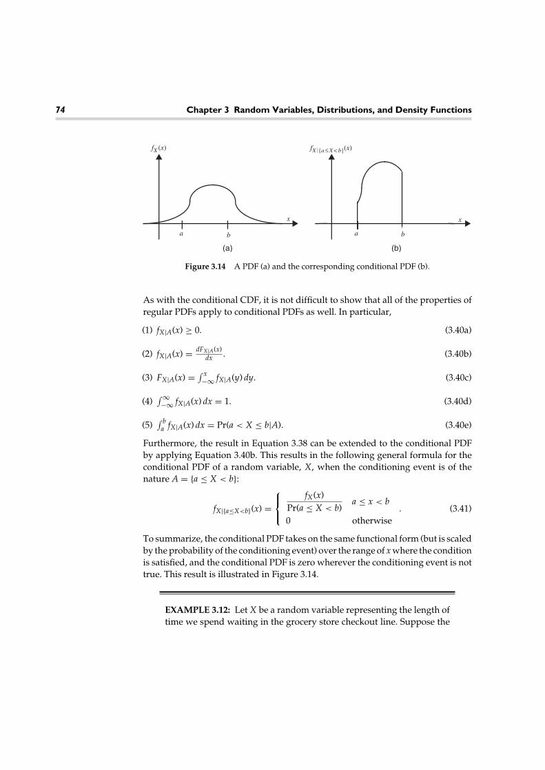
74 Chapter 3 Random Variables, Distributions, and Density Functions
a b a b
fX (x) fX{a ≤ X < b}(x)
x x
(a) (b)
Figure 3.14 A PDF (a) and the corresponding conditional PDF (b).
As with the conditional CDF, it is not difficult to show that all of the properties ofregular PDFs apply to conditional PDFs as well. In particular,
(1) fX|A(x) ≥ 0. (3.40a)
(2) fX|A(x) = dFX|A(x)dx . (3.40b)
(3) FX|A(x) = ∫ x−∞ fX|A(y) dy. (3.40c)
(4)∫ ∞−∞ fX|A(x) dx = 1. (3.40d)
(5)∫ b
a fX|A(x) dx = Pr(a < X ≤ b|A). (3.40e)
Furthermore, the result in Equation 3.38 can be extended to the conditional PDFby applying Equation 3.40b. This results in the following general formula for theconditional PDF of a random variable, X, when the conditioning event is of thenature A = {a ≤ X < b}:
fX|{a≤X<b}(x) =
fX(x)Pr(a ≤ X < b)
a ≤ x < b
0 otherwise. (3.41)
To summarize, the conditional PDF takes on the same functional form (but is scaledby the probability of the conditioning event) over the range of x where the conditionis satisfied, and the conditional PDF is zero wherever the conditioning event is nottrue. This result is illustrated in Figure 3.14.
EXAMPLE 3.12: Let X be a random variable representing the length oftime we spend waiting in the grocery store checkout line. Suppose the

3.5 Conditional Distribution and Density Functions 75
random variable X has an exponential PDF given by fX(x) =(1/c) exp(−x/c)u(x), where c = 3 minutes. What is the PDF for theamount of time we spend waiting in line given that we have alreadybeen waiting for 2 minutes? Here the conditioning event is of the formX > 2. We can use the result in Equation 3.41 by letting a = 2 and b = ∞.The probability of the conditioning event is Pr(X > 2) = 1 − FX(2) =exp(−2/3). Therefore, the conditional PDF is
fX|{X>2}(x) = exp(2/3)fX(x)u(x − 2) = 13
exp(
−x − 23
)u(x − 2).
It is curious to note that for this example, fX|{X>2}(x) = fX(x − 2). Thatis, given that we have been waiting in line for 2 minutes, the PDF ofthe total time we must wait in line is simply shifted by 2 minutes. Thisinteresting behavior is unique to the exponential distribution and wemight not have seen the same result if we had started with a differentdistribution. For example, try working the same problem starting witha Rayleigh distribution.
Up to this point, we have primarily looked at conditioning events that impose anumerical constraint. It is also common to consider conditioning events of a qual-itative, or nonnumerical, nature. Consider, for example, a random variable X thatrepresents a student’s score on a certain standardized test (e.g., the SAT or GRE).We might be interested in determining if there is any gender bias in the test. Todo so we could compare the distribution of the variable X given that the studentis female, FX|F(x), with the distribution of the same variable given that the studentis male, FX|M(x). If these distributions are substantially different, then we mightconclude a gender bias exists and work to fix the bias in the exam. Naturally, wecould work with conditional PDFs fX|F(x) and fX|M(x) as well. Here, the condition-ing event is a characteristic of the experiment that may affect the outcome ratherthan a restriction on the outcome itself.
In general, consider a set of mutually exclusive and exhaustive conditioningevents, A1, A2, . . . , AN . Suppose we had access to the conditional CDFs, FX|An (x),where n = 1, 2, . . . , N, and wanted to find the unconditional CDF, FX(x). Accordingto the theorem of total probability (Theorem 2.6),
FX(x) = Pr(X ≤ x) =N∑
n=1
Pr(X ≤ x|An) Pr(An) =N∑
n=1
FX|An (x) Pr(An). (3.42)
Hence, the CDF of X (unconditional) can be found by forming a weighted sum ofthe conditional CDFs with the weights determined by the probabilities that each of
76 Chapter 3 Random Variables, Distributions, and Density Functions
the conditioning events is true. By taking derivatives of both sides of the previousequation, a similar result is obtained for conditional PDFs, namely,
fX(x) =N∑
n=1
fX|An (x) Pr(An) . (3.43)
We might also be interested in looking at things in the reverse direction. Thatis, suppose we observe that the random variable has taken on a value of X = x.Does the probability of the event An change? To answer this, we need to computePr(An|X = x). If X were a discrete random variable, we could do this by invokingthe results of Theorem 2.5
Pr(An|X = x) = Pr(X = x|An) Pr(An)Pr(X = x)
. (3.44)
In the case of continuous random variables, greater care must be taken since bothPr(X = x|An) and Pr(X = x) will be zero, resulting in an indeterminate expression.To avoid that problem, rewrite the event {X = x} as {x ≤ X < x + ε} and considerthe result in the limit as ε → 0:
Pr(An|x ≤ X < x + ε) = Pr(x ≤ X < x + ε|An) Pr(An)Pr(x ≤ X < x + ε)
. (3.45)
Note that for infinitesimal ε, Pr(x ≤ X < x + ε) = fX(x)ε and similarly Pr(x ≤ X <
x + ε|An) = fX|An (x)ε. Hence,
Pr(An|x ≤ X < x + ε) = fX|An (x)ε Pr(An)fX(x)ε
= fX|An (x) Pr(An)fX(x)
. (3.46)
Finally, passing to the limit as ε → 0 gives the desired result:
Pr(An|X = x) = limε→0
Pr(An|x ≤ X < x + ε) = fX|An (x) Pr(An)fX(x)
. (3.47)
We could also combine this result with Equation 3.43 to produce an extension toBayes’s theorem:
Pr(An|X = x) = fX|An (x) Pr(An)N∑
n=1fX|An (x) Pr(An)
. (3.48)
EXAMPLE 3.13: In a certain junior swimming competition, swimmersare placed in one of two categories based on their previous times so thatall children can compete against others of their own abilities. The fastest

3.6 Engineering Application: Reliability and Failure Rates 77
swimmers are placed in the A category, while the slower swimmers areput in the B group. Let X be a random variable representing a child’stime (in seconds) in the 50-meter, freestyle race. Suppose that it is deter-mined that for those swimmers in group A, the PDF of a child’s timeis given by fX|A(x) = (4π )−1/2 exp(−(x − 40)2/4), while for those inthe B group the PDF is given by fX|B(x) = (4π )−1/2 exp(−(x − 45)2/4).Furthermore, assume that 30 percent of the swimmers are in the A groupand 70 percent are in the B group. If a child swims the race with a timeof 42 seconds, what is the probability that the child was in the B group?Applying Equation 3.48, we get
Pr(B|X = 42) = 0. 7fX|B(42)0. 3fX|A(42) + 0. 7fX|B(42)
= 0. 7 exp(−9/4)0. 3 exp(−1) + 0. 7 exp(−9/4)
= 0. 4007.
Naturally, the probability of the child being from group A must then bePr(A|X = 42) = 1 − Pr(B|X = 42) = 0. 5993.
3.6 Engineering Application: Reliabilityand Failure Rates
The concepts of random variables presented in this chapter are used extensivelyin the study of system reliability. Consider an electronic component that is to beassembled with other components as part of a larger system. Given a probabilisticdescription of the lifetime of such a component, what can we say about the lifetimeof the system itself? The concepts of reliability and failure rates are introduced inthis section to provide tools to answer such questions.
DEFINITION 3.6: Let X be a random variable that represents the lifetime of adevice. That is, if the device is turned on at time zero, X would represent the timeat which the device fails. The reliability function of the device, RX(t), is simply theprobability that the device is still functioning at time t:
RX(t) = Pr(X > t). (3.49)
Note that the reliability function is just the complement of the CDF of the randomvariable. That is, RX(t) = 1 − FX(t). As it is often more convenient to work with

78 Chapter 3 Random Variables, Distributions, and Density Functions
PDFs rather than CDFs, we note that the derivative of the reliability function canbe related to the PDF of the random variable X by R′
X(t) = −fX(t).With many devices, the reliability changes as a function of how long the device
has been functioning. Suppose we observe that a particular device is still function-ing at some point in time, t. The remaining lifetime of the device may behave (in aprobabilistic sense) very differently from when it was first turned on. The conceptof failure rate is used to quantify this effect.
DEFINITION 3.7: Let X be a random variable that represents the lifetime of adevice. The failure rate function is
r(t) = fX|{X>t}(x)|x=t . (3.50)
To give this quantity some physical meaning, we note that Pr(t < X < t + dt|X > t) =r(t)dt. Thus, r(t)dt is the probability that the device will fail in the next time instantof length dt, given that the device has survived up to now (time t). Different typesof “devices” have failure rates that behave in different manners. Our pet goldfish,Elvis, might have an increasing failure rate function (as do most biological crea-tures). That is, the chances of Elvis “going belly up” in the next week is greaterwhen Elvis is six months old than when he is just one month old. We could alsoimagine devices that have a decreasing failure rate function (at least for part oftheir lifetime). For example, an integrated circuit might be classified into one oftwo types, those fabricated correctly with expected long lifetimes and those withdefects which generally fail fairly quickly. When we select an IC, we may not knowwhich type it is. Once the device lives beyond that initial period when the defectiveICs tend to fail, the failure rate may go down (at least for a while). Finally, theremay be some devices whose failure rates remain constant with time.
The failure rate of a device can be related to its reliability function. FromEquation 3.41, it is noted that
fX|{X>t}(x) = fX(x)u(x − t)1 − Fx(t)
. (3.51)
The denominator in this expression is the reliability function, RX(t), while the PDFin the numerator is simply −R′
X(x). Evaluating at x = t produces the failure ratefunction
r(t) = −R′X(t)
RX(t). (3.52)
Conversely, given a failure rate function, r(t), one can solve for the reliabilityfunction by solving the first order differential equation:
ddt
Rx(t) = −r(t) RX(t). (3.53)

3.6 Engineering Application: Reliability and Failure Rates 79
The general solution to this differential equation (subject to the initial conditionRx(0) = 1) is
RX(t) = exp[−
∫ t
0r(u)du
]u(t). (3.54)
It is interesting to note that a failure rate function completely specifies the PDF ofa device’s lifetime:
fX(t) = −R′X(t) = r(t) exp
(−
∫ t
0r(u)du
)u(t). (3.55)
For example, suppose a device had a constant failure rate function, r(t) = λ.The PDF of the device’s lifetime would then follow an exponential distribution,fX(t) = λ exp(−λt) u(t). The corresponding reliability function would also be expo-nential, RX(t) = exp(−λt) u(t). We say that the exponential random variable hasthe memoryless property. That is, it does not matter how long the device has beenfunctioning, the failure rate remains the same.
EXAMPLE 3.14: Suppose the lifetime of a certain device follows aRayleigh distribution given by fX(t) = 2btexp(−bt2)u(t). What are thereliability function and the failure rate function? The reliability functionis given by
RX(t) = Pr(X > t) =[∫ ∞
t2buexp(−bu2)du
]u(t) = exp(−bt2)u(t).
A straightforward application of Equation 3.52 produces the failure ratefunction, r(t) = 2bt u(t). In this case, the failure rate is linearly increasingin time.
Next, suppose we have a system which consists of N components, each of whichhas a lifetime described by the random variable Xn, n = 1, 2, . . . , N. Furthermore,assume that for the system to function, all N components must be functioning. Inother words, if any of the individual components fails, the whole system fails. Thisis usually referred to as a series connection of components. If we can characterizethe reliability and failure rate functions of each individual component, can wecalculate the same functions for the entire system? The answer is yes, under somemild assumptions. Define X to be the random variable representing the lifetime ofthe system. Then
X = min(X1, X2, . . . , XN). (3.56)

80 Chapter 3 Random Variables, Distributions, and Density Functions
Furthermore,
RX(t) = Pr(X > t)
= Pr({X1 > t} ∩ {X2 > t} ∩ · · · ∩ {XN > t}). (3.57)
We assume that all of the components fail independently. That is, the event {Xi > t}is taken to be independent of {Xj > t} for all i �= j. Under this assumption,
RX(t) = Pr(X1 > t) Pr(X2 > t) · · · Pr(XN > t)
= RX1 (t) RX2 (t) · · · RXN (t). (3.58)
Furthermore, application of Equation 3.52 provides an expression for the failurerate function:
r(t) = −R′X(t)
RX(t)= −
ddt
[RX1 (t)RX2 (t) · · · RXN (t)]RX1 (t)RX2 (t) · · · RXN (t)
(3.59)
= −N∑
n=1
R′Xn
(t)
RXn (t)=
N∑n=1
rn(t), (3.60)
where rn(t) is the failure rate function of the nth component. We have shown thatfor a series connection of components, the reliability function of the system is theproduct of the reliability functions of each component and the failure rate functionof the system is the sum of the failure rate functions of the individual components.
We may also consider a system that consists of a parallel interconnection ofcomponents. That is, the system will be functional as long as any of the componentsare functional. We can follow a similar derivation to compute the reliability andfailure rate functions for the parallel interconnection system. First, the reliabilityfunction is written as
RX(t) = Pr({X1 > t} ∪ {X2 > t} ∪ · · · ∪ {XN > t}). (3.61)
In this case, it is easier to work with the complement of the reliability function (theCDF of the lifetime). Since the reliability function represents the probability thatthe system is still functioning at time t, the complement of the reliability functionrepresents the probability that the system is not working at time t. With the parallelinterconnections, the system will fail only if all the individual components fail.Hence,
1 − RX(t) = Pr(X ≤ t) = Pr({X1 ≤ t} ∩ {X2 ≤ t} ∩ · · · ∩ {XN ≤ t})= Pr(X1 ≤ t) Pr(X2 ≤ t) · · · Pr(XN ≤ t)
= (1 − RX1 (t))(1 − RX2 (t)) · · · (1 − RXN (t)). (3.62)

3.6 Engineering Application: Reliability and Failure Rates 81
As a result, the reliability function of the parallel interconnection system isgiven by
RX(t) = 1 −N∏
n=1
(1 − RXn (t)). (3.63)
Unfortunately, the general formula for the failure rate function is not as simple asin the serial interconnection case. Application of Equation 3.52 to our precedingequation gives (after some straightforward manipulations)
r(t) = −1 − RX(t)RX(t)
N∑n=1
R′Xn
(t)
1 − RXn (t), (3.64)
or, equivalently,
r(t) =[
1RX(t)
− 1] N∑
n=1
rn(t)1
RXn (t)− 1
. (3.65)
EXAMPLE 3.15: Suppose a system consists of N components each witha constant failure rate, rn(t) = λn, n = 1, 2, . . . , N. Find the reliabilityand failure rate functions for a series interconnection. Then find the samefunctions for a parallel interconnection. It was shown previously that aconstant failure rate function corresponds to an exponential reliabilityfunction. That is, RXn (t) = exp(−λnt)u(t). For the serial interconnection,we then have
RX(t) =N∏
n=1
RXn (t) =N∏
n=1
exp(−λnt)u(t) = exp
(−
[ N∑n=1
λn
]t
)u(t),
r(t) =N∑
n=1
rn(t) =N∑
n=1
λn.
For the parallel interconnection,
RX(t) ={
1 −N∏
n=1
[1 − exp(−λnt)]
}u(t),
r(t) =
N∏n=1
[1 − exp(−λnt)]
1 −N∏
n=1[1 − exp(−λnt)]
N∑n=1
λn
exp(λnt) − 1.
82 Chapter 3 Random Variables, Distributions, and Density Functions
Exercises3.1 Suppose a random variable is equally likely to fall anywhere in the interval
[a, b]. Then the PDF is of the form
fX(x) =
1b − a
a ≤ x ≤ b
0 otherwise.
Find and sketch the corresponding CDF.
3.2 Find and plot the CDFs corresponding to each of the following PDFs:
(a) fX(x) =
1 0 ≤ x < 1
0 otherwise.
(b) fX(x) =
x 0 ≤ x < 1
2 − x 1 ≤ x < 2
0 otherwise
.
3.3 A random variable has the following exponential PDF:
fX(x) =
a−bx x ≤ 0
0 otherwise,
where a and b are constants.
(a) Determine the required relationship between a and b.(b) Determine the corresponding CDF.
3.4 A certain random variable has a probability density function of the formfX(x) = ce−2xu(x). Find the following:
(a) the constant c,(b) Pr(X > 2),(c) Pr(X < 3),(d) Pr(X < 3|X > 2).
3.5 Repeat Problem 3.4 using the PDF fX(x) = cx2 + 4
.
Exercises 83
3.6 Repeat Problem 3.4 using the PDF fX(x) = c√25 − x2
, −5 < x < 5.
3.7 The voltage of communication signal S is measured. However, themeasurement procedure is corrupted by noise resulting in a random mea-surement with the PDF shown in the accompanying diagram. Find theprobability that for any particular measurement, the error will exceed±0. 75 percent of the correct value if this correct value is 10 volts.
10.1
10
fS(s)
s
9.9
3.8 Prove the integral identity, I =∫ ∞
−∞exp
(−x2
2
)dx = √
2π . Hint: It may
be easier to show that I2 = 2π .
3.9 Using the normalization integral for a Gaussian random variable, find ananalytical expression for the following integral:
I =∫ ∞
−∞exp(−(ax2 + bx + c)) dx,
where a > 0, b, and c are constants.
3.10 A Gaussian random variable has a probability density function of the form
fX(x) = c exp(−(2x2 + 3x + 1)).
(a) Find the value of the constant c.(b) Find the values of the parameters m and σ for this Gaussian random
variable.
3.11 A Gaussian random variable has a PDF of the form
fX(x) = 1√50π
exp
(− (x − 10)2
50
).
Write each of the following probabilities in terms of Q-functions (withpositive arguments) and also give numerical evaluations.

84 Chapter 3 Random Variables, Distributions, and Density Functions
(a) Pr(X > 17)(b) Pr(X > 4)(c) Pr(X < 15)(d) Pr(X < −2)
(e) Pr(|X − 10| > 7)(f) Pr(|X − 10| < 3)(g) Pr(|X − 7| > 5)(h) Pr(|X − 4| < 7)
3.12 Prove the following properties of the Gamma function.
(a) �(n) = (n − 1)!, for n = 1, 2, 3, . . .
(b) �(x + 1) = x�(x)
(c) �(1/2) = √π
3.13 Prove the following properties of conditional CDFs.
(a) FX|A(−∞) = 0, FX|A(∞) = 1
(b) 0 ≤ FX|A(x) ≤ 1
(c) For x1 < x2, FX|A(x1) ≤ FX|A(x2)
(d) For x1 < x2, Pr(x1 < X ≤ x2|A) = FX|A(x2) − FX|A(x1)
3.14 Let X be a Gaussian random variable such that X ∼ N(0, σ 2). Find and plotthe following conditional PDFs.
(a) fX|X>0(x)
(b) fX∣∣|X|<3
(x)
(c) fX∣∣|X|>3
(x)
3.15 Mr. Hood is a good archer. He can regularly hit a target having a 3-ft.diameter and often hits the bull’s-eye, which is 0.5 ft. in diameter, from 50 ft.away. Suppose the miss is measured as the radial distance from the centerof the target and, further, that the radial miss distance is a Rayleigh randomvariable with the constant in the Rayleigh PDF being σ 2 = 4(sq. ft.).
(a) Determine the probability of Mr. Hood’s hitting the target.
(b) Determine the probability of Mr. Hood’s hitting the bull’s-eye.
(c) Determine the probability of Mr. Hood’s hitting the bull’s-eye giventhat he hits the target.
3.16 A digital communication system sends two messages, M = 0 or M = 1,with equal probability. A receiver observes a voltage which can be mod-eled as a Gaussian random variable, X, whose PDFs conditioned on the

Exercises 85
transmitted message are given by
fX|M=0(x) = 1√2πσ 2
exp
(− x2
2σ 2
)and
fX|M=1(x) = 1√2πσ 2
exp
(− (x − 1)2
2σ 2
).
(a) Find and plot Pr(M = 0|X = x) as a function of x for σ 2 = 1. Repeatfor σ 2 = 5.
(b) Repeat part (a) assuming that the a priori probabilities are Pr(M = 0) =1/4 and Pr(M = 1) = 3/4.
3.17 In Problem 3.16, suppose our receiver must observe the random variable Xand then make a decision as to what message was sent. Furthermore,suppose the receiver makes a three-level decision as follows:
(1) Decide 0 was sent if Pr(M = 0|X = x) ≥ 0. 9.
(2) Decide 1 was sent if Pr(M = 1|X = x) ≥ 0. 9.
(3) Erase the symbol (decide not to decide) if both Pr(M = 0|X = x) < 0. 9and Pr(M = 1|X = x) < 0. 9.
Assuming the two messages are equally probable, Pr(M = 0) = Pr(M =1) = 1/2, and that σ 2 = 1, find
(a) the range of x over which each of the three decisions should be made,
(b) the probability that the receiver erases a symbol,
(c) the probability that the receiver makes an error (i.e., decides a 0 wassent when a 1 was actually sent, or vice versa).
3.18 Recalling Example 3.15, suppose that a serial connection system has10 components and the failure rate function is the same constant for allcomponents and is 1 per 100 days.
(a) Determine the probability that the lifetime of the system exceeds10 days.
(b) What is the probability that the lifetime of one component exceeds10 days?
(c) What is the reliability function of each component and of the systemas a whole?

86 Chapter 3 Random Variables, Distributions, and Density Functions
MATLAB Exercises3.19 Write a MATLAB program to calculate the probability Pr(x1 ≤ X ≤ x2)
if X is a Gaussian random variable for an arbitrary x1 and x2. Note thatyou will have to specify the mean and variance of the Gaussian randomvariable.
3.20 Write a MATLAB program to calculate the probability Pr(|X − a| < b) ifX is a Gaussian random variable for an arbitrary a and b > 0. Note thatyou will have to specify the mean and variance of the Gaussian randomvariable.
3.21 Use the MATLAB rand function to create a random variable X uniformlydistributed over (0, 1). Then create a new random variable according toY = − ln(X). Repeat this procedure many times to create a large numberof realizations of Y. Using these samples, estimate and plot the probabil-ity density function of Y. Find an analytical model that seems to fit yourestimated PDF.
3.22 Use the MATLABrandn function to create a Gaussian distributed randomvariable X. Repeat this procedure and form a new random variable Y.Finally, form a random variable Z according to Z =
√X2 + Y2. Repeat this
procedure many times to create a large number of realizations of Z. Usingthese samples, estimate and plot the probability density function of Z. Findan analytical model that seems to fit your estimated PDF.
3.23 Use the MATLAB randn function to generate a large number of sam-ples according to a Gaussian distribution. Let A be the event A = {thesample is greater than 1.5}. Of those samples that are members of theevent A, what proportion (relative frequency) is greater than 2. By com-puting this proportion you will have estimated the conditional probabilityPr(X > 2|X > 1. 5). Calculate the exact conditional probability analyticallyand compare it with the numerical results obtained through your MATLABprogram.

Operations on a SingleRandom Variable 4
In our study of random variables we use the probability density function or thecumulative distribution function to provide a complete statistical description ofthe random variable. From these functions we could, in theory, determine justabout anything we might want to know about the random variable. In many cases,it is of interest to distill this information down to a few parameters that describesome of the important features of the random variable. For example, we saw inChapter 3 that the Gaussian random variable is described by two parameters, whichwere referred to as the mean and variance. In this chapter, we will look at theseparameters as well as several others that describe various characteristics of ran-dom variables. We will see that these parameters can be viewed as the results ofperforming various operations on a random variable.
4.1 Expected Value of a Random Variable
To begin, we introduce the idea of an average or expected value of a randomvariable. This is perhaps the single most important characteristic of a randomvariable and is also a concept very familiar to most students. After taking a test, oneof the most common questions a student will ask after they see their grade is, Whatwas the average? On the other hand, how often does a student ask, What was theprobability density function of the exam scores? While the answer to the secondquestion would provide the student with more information about how the classperformed, the student may not want all that information. Just knowing the averagemay be sufficient to tell the student how he or she performed relative to the rest ofthe class.
87

88 Chapter 4 Operations on a Single Random Variable
DEFINITION 4.1: The expected value of a random variable X which has a PDF,fX(x), is
E[X] =∫ ∞
−∞xfX(x) dx. (4.1)
The terms average, mean, expectation, and first moment are all alternative names forthe concept of expected value and will be used interchangeably throughout the text.Furthermore, an overbar is often used to denote expected value so that the symbolX is to be interpreted as meaning the same thing as E[X]. Another commonly usednotation is to write µX = E[X].
For discrete random variables, the PDF can be written in terms of the probabilitymass function,
fX(x) =∑
k
PX(xk)δ(x − xk). (4.2)
In this case, using the properties of delta functions, the definition of expected valuesfor discrete random variables reduces to
E[X] =∑
k
xkPX(xk). (4.3)
Hence, the expected value of a discrete random variable is simply a weighted aver-age of the values that the random variable can take on, weighted by the probabilitymass of each value. Naturally, the expected value of a random variable exists onlyif the integral in Equation 4.1 or the series in Equation 4.3 converges. One can dreamup many random variables for which the integral or series does not converge andthus their expected values don’t exist (or less formally, their expected value is infi-nite). To gain some physical insight into this concept of expected value, we maythink of fX(x) as a mass distribution of an object along the x-axis; then Equation 4.1calculates the centroid or center of gravity of the mass.
EXAMPLE 4.1: Consider a random variable that has an exponential
PDF given by fX(x) = 1b
exp(−x
b
)u(x). Its expected value is calculated
as follows:
E[X] =∫ ∞
0
xb
exp(−x
b
)dx = b
∫ ∞
0yexp(−y)dy = b.
The last equality in the series is obtained by using integration by partsonce. It is seen from this example that the parameter b that appears inthis exponential distribution is, in fact, the mean (or expected value) ofthe random variable.
4.1 Expected Value of a Random Variable 89
EXAMPLE 4.2: Next, consider a Poisson random variable whose prob-ability mass function is given by PX(k) = αke−α/k!, k = 0, 1, 2, . . . . Itsexpected value is found in a similar manner.
E[X] =∞∑
k=0
kαke−α
k! = e−α∞∑
k=1
αk
(k − 1)! = αe−α∞∑
k=1
αk−1
(k − 1)!
= αe−α∞∑
m=0
αm
m! = αe−αeα = α
Once again, we see that the parameter α in the Poisson distribution isequal to the mean.
EXAMPLE 4.3: In the last two examples, we saw that a random variablewhose PDF or PMF was described by a single parameter in both casesturned out to be the mean. We work one more example here to show thatthis does not always have to be the case. Consider a Rayleigh randomvariable with PDF
fX(x) = xσ 2 exp
(− x2
2σ 2
)u(x).
The mean is calculated as follows:
E[X] =∫ ∞
0
x2
σ 2 exp
(− x2
2σ 2
)dx = √
2σ
∫ ∞
0y1/2exp(−y)dy
= √2 σ�(3/2) =
√π
2σ .
The last equality is obtained using the fact that �(3/2) = √π/2. Alter-
natively (for those students not familiar with the properties of gammafunctions), one could obtain this result using integration by parts onceon the original integral (setting u = x and dv = (x/σ 2) exp(−x2/(2σ 2))).In this case, neither the parameter σ nor σ 2 is equal to the expectedvalue of the random variable. However, since the mean is proportionalto σ , we could, if we wanted to, rewrite the Rayleigh PDF in terms ofits expected value, µX , as follows:
fX(x) = πx
2µ2X
exp
(− πx2
4µ2X
)u(x).

90 Chapter 4 Operations on a Single Random Variable
4.2 Expected Values of Functions ofRandom Variables
The concept of expectation can be applied to functions of random variables as wellas to the random variable itself. This will allow us to define many other parametersthat describe various aspects of a random variable.
DEFINITION 4.2: Given a random variable X with PDF fX(x), the expected valueof a function, g(X), of that random variable is given by
E[g(X)] =∫ ∞
−∞g(x)fX(x) dx. (4.4)
For a discrete random variable, this definition reduces to
E[g(X)] =∑
k
g(xk)PX(xk). (4.5)
To start with, we demonstrate one extremely useful property of expectations inthe following theorem.
THEOREM 4.1: For any constants a and b,
E[aX + b] = aE[X] + b. (4.6)
Furthermore, for any function g(x) that can be written as a sum of several otherfunctions (i.e., g(x) = g1(x) + g2(x) + · · · + gN(x)),
E
[ N∑k=1
gk(X)
]=
N∑k=1
E[gk(X)] (4.7)
In other words, expectation is a linear operation and the expectation operator canbe exchanged (in order) with any other linear operation.
PROOF: The proof follows directly from the linearity of the integration operator.
E[aX + b] =∫ ∞
−∞(ax + b)fX(x) dx
= a∫ ∞
−∞xfX(x) dx + b = aE[X] + b. (4.8)
The second part of the theorem is proved in an identical manner:
E
[ N∑k=1
gk(X)
]=
∫ ∞
−∞
[ N∑k=1
gk(x)
]fX(x) dx =
N∑k=1
∫ ∞
−∞gk(x)fX(x) dx =
N∑k=1
E[gk(X)].
(4.9)
�

4.3 Moments 91
Table 4.1 Expected Values of Various Functions of Random Variables
Name Function of X Expected value, notation
Mean, average, expectedvalue, expectation, firstmoment
g(x) = x µX = X = E[X]
nth moment g(x) = xn Xn = E[Xn]nth central moment g(x) = (x − µX)n (X − µX)n = E[(X − µX)n]Variance g(x) = (x − µX)2 σ 2
X = E[(X − µX)2]
Coefficient of skewness g(x) =(
x − µXσX
)3cs = E
[(X − µX
σX
)3]
Coefficient of kurtosis g(x) =(
x − µXσX
)4ck = E
[(X − µX
σX
)4]
Characteristic function g(x) = ejωx �X(ω) = E[ejωX]Moment generating function g(x) = esx MX(s) = E[esX]Probability generatingfunction
g(x) = zx HX(z) = E[zX]
Different functional forms of g(X) lead to various different parameters thatdescribe the random variable and are known by special names. A few of the morecommon ones are listed in Table 4.1. In the following sections, selected parameterswill be studied in more detail.
4.3 Moments
DEFINITION 4.3: The nth moment of a random variable X is defined as
E[Xn] =∫ ∞
−∞xnfX(x) dx. (4.10)
For a discrete random variable, this definition reduces to
E[Xn] =∑
k
xnk PX(xk). (4.11)
The zeroth moment is simply the area under the PDF and hence must be 1 forany random variable. The most commonly used moments are the first and second

92 Chapter 4 Operations on a Single Random Variable
moments. The first moment is what we previously referred to as the mean, whilethe second moment is the mean squared value. For some random variables, thesecond moment might be a more meaningful characterization than the first. Forexample, suppose X is a sample of a noise waveform. We might expect that thedistribution of the noise is symmetric about zero (i.e., just as likely to be positiveas negative) and hence the first moment will be zero. So if we are told that X has azero mean, this merely says that the noise does not have a bias. On the other hand,the second moment of the random noise sample is in some sense a measure of thestrength of the noise. In fact, in a later Chapter 10, we will associate the secondmoment of a noise process with the power in the process. Hence, specifying thesecond moment can give us some useful physical insight into the noise process.
EXAMPLE 4.4: Consider a discrete random variable that has a binomialdistribution. Its probability mass function is given by
PX(k) =(
nk
)pk(1 − p)n−k, k = 0, 1, 2, . . . , n.
The first moment is calculated as follows:
E[X]=n∑
k=0
k(
nk
)pk(1−p)n−k =
n∑k=1
kn!k!(n−k)!pk(1−p)n−k
=n∑
k=1
n!(k−1)!(n−k)!pk(1−p)n−k =np
n∑k=1
(n−1)!(k−1)!(n−k)!pk−1(1−p)n−k
=npn∑
k=1
(n−1k−1
)pk−1(1−p)n−k =np
n−1∑m=0
(n−1
m
)pm(1−p)n−1−m.
In this last expression, the summand is a valid probability mass function(i.e., that of a binomial random variable with parameters p and n − 1)and hence must sum to unity. Therefore, E[X] = np. To calculate thesecond moment, we employ a helpful little trick. Note that we can writek2 = k(k − 1) + k. Then
E[X2] =n∑
k=0
k2(
nk
)pk(1 − p)n−k
=n∑
k=0
k(k − 1)(
nk
)pk(1 − p)n−k +
n∑k=0
k(
nk
)pk(1 − p)n−k.

4.3 Moments 93
The second sum is simply the first moment, which has already beencalculated. The first sum is evaluated in a manner similar to that usedto calculate the mean.
n∑k=0
k(k − 1)(
nk
)pk(1 − p)n−k =
n∑k=2
n!(k − 2)!(n − k)!pk(1 − p)n−k
= n(n − 1)p2n∑
k=2
(n − 2)!(k − 2)!(n − k)!pk−2(1 − p)n−k
= n(n − 1)p2n∑
k=2
(n − 2k − 2
)pk−2(1 − p)n−k
= n(n − 1)p2n−2∑m=0
(n − 2
m
)pm(1 − p)n−2−m = n(n − 1)p2
Putting these two results together gives
E[X2] = n(n − 1)p2 + np = n2p2 + np(1 − p).
EXAMPLE 4.5: Consider a random variable with a uniform probabilitydensity function given as
fX(x) ={
1/a 0 ≤ x ≤ a
0 otherwise
The mean is given by
E[X] =∫ a
0
xa
dx = x2
2a
∣∣∣∣a
0= a
2,
while the second moment is
E[X2] =∫ a
0
x2
adx = x3
3a
∣∣∣∣a
0= a2
3.
In fact, it is not hard to see that in general, the nth moment of this uniformrandom variable is given by
E[Xn] =∫ a
0
xn
adx = xn+1
(n + 1)a
∣∣∣∣a
0= an
n + 1.

94 Chapter 4 Operations on a Single Random Variable
4.4 Central Moments
Consider a random variable Y which could be expressed as the sum, Y = a+X of adeterministic (i.e., not random) part a and a random part X. Furthermore, supposethat the random part tends to be very small compared to the fixed part. That is, therandom variable Y tends to take small fluctuations about a constant value, a. Suchmight be the case in a situation where there is a fixed signal corrupted by noise.In this case, we might write Yn = (a + X)n ≈ an. In this case, the nth moment ofY would be dominated by the fixed part. That is, it’s difficult to characterize therandomness in Y by looking at the moments. To overcome this, we can use theconcept of central moments.
DEFINITION 4.4: The nth central moment of a random variable X is defined as
E[(X − µX)n] =∫ ∞
−∞(x − µX)nfX(x) dx. (4.12)
In this equation, µX is the mean (first moment) of the random variable. For discreterandom variables, this definition reduces to
E[(X − µX)n] =∑
k
(xk − µX)kPX(xk). (4.13)
With central moments, the mean is subtracted from the variable before the momentis taken in order to remove the bias in the higher moments due to the mean. Notethat, like regular moments, the zeroth central moment is E[(X − µX)0] = E[1] = 1.Furthermore, the first central moment is E[X − µX] = E[X] − µX = µX − µX = 0.Therefore, the lowest central moment of any real interest is the second centralmoment. This central moment is given a special name, the variance, and we quiteoften use the notation σ 2
X to represent the variance of the random variable X. Notethat
σ 2X = E[(X − µX)2] = E[X2 − 2µXX + µ2
X] = E[X2] − 2µXE[X] + µ2X
= E[X2] − µ2X . (4.14)
In many cases, the best way to calculate the variance of a random variable is tocalculate the first two moments and then form the second moment minus the firstmoment squared.
EXAMPLE 4.6: For the binomial random variable in Example 4.4, recallthat the mean was E[X] = np and the second moment was E[X2] =n2p2 + np(1 − p). Therefore, the variance is given by σ 2
X = np(1 − p).

4.4 Central Moments 95
Similarly, for the uniform random variable in Example 4.5, E[X] = a/2,E[X2] = a2/3, and hence σ 2
X = a2/3 − a2/4 = a2/12. Note that if themoments have not previously been calculated, it may be just as easyto compute the variance directly. In the case of the uniform randomvariable, once the mean has been calculated, the variance can befound as
σ 2X =
∫ a
0(x − a/2)2 1
adx =
∫ a/2
−a/2
x2
adx = x3
3a
∣∣∣∣a/2
−a/2= a2
12.
Another common quantity related to the second central moment of a ran-dom variable is the standard deviation, which is defined as the square root of thevariance,
σX =√
E[(X − µX)2].
Both the variance and the standard deviation serve as a measure of the width ofthe PDF of a random variable. Some of the higher order central moments alsohave special names, although they are much less frequently used. The third centralmoment is known as the skewness and is a measure of the symmetry of the PDFabout the mean. The fourth central moment is called the kurtosis and is a measureof the peakedness of a random variable near the mean. Note that not all randomvariables have finite moments and/or central moments. We give an example ofthis later for the Cauchy random variable. Some quantities related to these higherorder central moments are given in Definition 4.5.
DEFINITION 4.5: The coefficient of skewness is
cs = E[(X − µX)3]σ 3
X
. (4.15)
This is a dimensionless quantity that is positive if the random variable has a PDFskewed to the right and negative if skewed to the left. The coefficient of kurtosis isalso dimensionless and is given as
ck = E[(X − µX)4]σ 4
X
. (4.16)
The more the PDF is concentrated near its mean, the larger the coefficient ofkurtosis. In other words, a random variable with a large coefficient of kurtosiswill have a large peak near the mean.

96 Chapter 4 Operations on a Single Random Variable
EXAMPLE 4.7: An exponential random variable has a PDF given by
fX(x) = b exp(−bx)u(x).
The mean value of this random variable is µX = 1/b. The nth centralmoment is given by
E[(X − µX)n] =∫ ∞
0(x − 1/b)nb exp(−bx)dx
= be
∫ ∞
− 1b
yn exp(−by)dy
= 1bn
n∑m=0
n!m! (−1)m.
In the preceding expression, it is understood that 0! = 1. As expected,it is easily verified from the expression that the zeroth central momentis 1 and the first central moment is 0. Beyond these, the second centralmoment is σ 2
X = 1/b2, the third central moment is E[(X−1/b)3] = −2/b3,and the fourth central moment is E[(X − 1/b)4] = 9/b4. The coefficientsof skewness and kurtosis are given by
cs = E[(X − µX)3]σ 3
X
= −2/b3
1/b3 = −2,
ck = E[(X − µX)4]σ 4
X
= 9/b4
1/b4 = 9.
The fact that the coefficient of skewness is negative shows that theexponential PDF is skewed to the left of its mean.
EXAMPLE 4.8: Next consider a Laplace (two-sided exponential) ran-dom variable with a PDF given by
fX(x) = b2
exp(−b|x|).Since this PDF is symmetric about zero, its mean is zero, and hence inthis case the central moments are simply the moments
E[(X − µX)n] = E[Xn] =∫ ∞
−∞bxn
2exp(−b|x|) dx.

4.4 Central Moments 97
Since the two-sided exponential is an even function and xn is an oddfunction for any odd n, the integrand is then an odd function for anyodd n. The integral of any odd function over an interval symmetric aboutzero is equal to zero, and hence all odd moments of the Laplace randomvariable are zero. The even moments can be calculated individually:
σ 2X =E[X2]=
∫ ∞
−∞bx2
2exp(−b|x|)dx=
∫ ∞
0bx2 exp(−bx)dx= 2
b2 ,
E[(X−µX)4]=E[X4]=∫ ∞
−∞bx4
2exp(−b|x|)dx=
∫ ∞
0bx4 exp(−bx)dx= 24
b4 .
The coefficient of skewness is zero (since the third central moment iszero) and the coefficient of kurtosis is
ck = E[(X − µX)4]σ 4
X
= 24/b4
4/b4 = 6.
Note that the Laplace distribution has a sharp peak near its mean asevidenced by a large coefficient of kurtosis. The fact that the coefficientof skewness is zero is consistent with the fact that the distribution issymmetric about its mean.
EXAMPLE 4.9: It is often the case that the PDF of random vari-ables of practical interest may be too complicated to allow us tocompute various moments and other important parameters of thedistribution in an analytic fashion. In those cases, we can use a
computer to calculate the needed quantities numerically. Take, for example,a Rician random variable whose PDF is given by
fX(x) = xσ 2 exp
(−x2 + a2
2σ 2
)Io
( axσ 2
)u(x).
Suppose we wanted to know the mean of this random variable. This requiresus to evaluate:
µX =∫ ∞
0
x2
σ 2 exp
(−x2 + a2
2σ 2
)Io
( axσ 2
)dx.
Note that the parameter σ 2 that shows up in the Rician PDF is not the varianceof the Rician random variable. While analytical evaluation of this integral

98 Chapter 4 Operations on a Single Random Variable
looks formidable, given numerical values for a and σ 2, this integral canbe evaluated (at least approximately) using standard numerical integra-tion techniques. In order to use the numerical integration routines builtinto MATLAB, we must first write a function that evaluates the integrand.For evaluating the mean of the Rician PDF, this can be accomplished asfollows: (see Appendix D, (D.52) for the analytic expression for the mean.)
function pdf=Rician_mean(x,a,sigma)
% Evaluate the integrand needed for calculating the mean of a
% Rician random variable with parameters a and sigma.
pdf=(x./sigma).∧2.*exp(-(x.∧2+a∧2)/(2*sigma∧2));pdf=pdf.*besseli(0,a*x/sigma∧2);
Once this function is defined, the MATLAB function quad8 can be calledupon to perform the numerical integration. For example, if a = 2 and σ = 3,the mean could be calculated as follows:
a=2; sigma=3; % set parameters
limit1=0; limit2=20; % set limits of integration.
mean=quad8(‘Rician_mean’,limit1,limit2,[],[],a,sigma);
Executing this code produced an answer of µX = 4. 1665. Note that in orderto calculate the mean, the upper limit of the integral should be infinite.However, using limit2=Inf in the preceding code would have led MAT-LAB to produce a result of NaN (“not a number”). Instead, we must use anupper limit sufficiently large that for the purposes of evaluating the inte-gral it is essentially infinite. This can be done by observing the integrandand seeing at what point the integrand dies off. The reader is encouragedto execute the code in this example using different values of the upper inte-gration limit to see how large the upper limit must be to produce accurateresults.
4.5 Conditional Expected Values
Another important concept involving expectation is that of conditional expectedvalue. As specified in Definition 4.6, the conditional expected value of a randomvariable is a weighted average of the values the random variable can take on,weighted by the conditional PDF of the random variable.

4.5 Conditional Expected Values 99
DEFINITION 4.6: The expected value of a random variable X, conditioned onsome event A is
E[X|A] =∫ ∞
−∞xfX|A(x) dx. (4.17)
For a discrete random variable, this definition reduces to
E[X|A] =∑
k
xkPX|A(xk). (4.18)
Similarly, the conditional expectation of a function, g(·), of a random variable,conditioned on the event A is
E[g(X)|A] =∫ ∞
−∞g(x)fX|A(x) dx or E[g(X)|A] =
∑k
g(xk)PX|A(xk), (4.19)
depending on whether the random variable is continuous or discrete.
Conditional expected values are computed in the same manner as regular expectedvalues with the PDF or PMF replaced by a conditional PDF or conditional PMF.
EXAMPLE 4.10: Consider a Gaussian random variable of the form
fX(x) = 1√2π
exp
(−x2
2
).
Suppose the event A is that the random variable X is positive,A = {X > 0}. Then
fX|A(x) = fX(x)Pr(X > 0)
u(x) =√
2π
exp
(−x2
2
)u(x).
The conditional expected value of X given that X > 0 is then
E[X|X > 0] =∫ ∞
−∞xfX|X>0(x) dx =
√2π
∫ ∞
0x exp
(−x2
2
)dx
= −√
2π
exp
(−x2
2
) ∣∣∣∣∞
0=
√2π
.
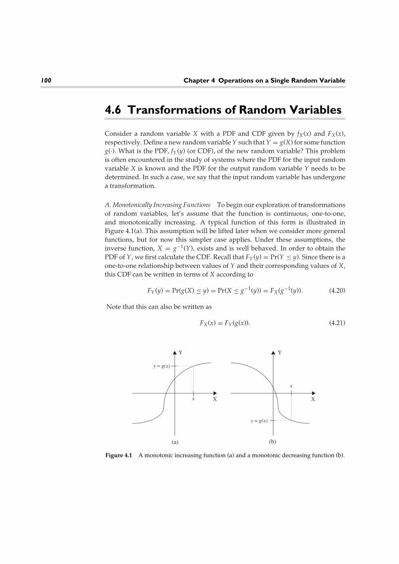
100 Chapter 4 Operations on a Single Random Variable
4.6 Transformations of Random Variables
Consider a random variable X with a PDF and CDF given by fX(x) and FX(x),respectively. Define a new random variable Y such that Y = g(X) for some functiong(·). What is the PDF, fY(y) (or CDF), of the new random variable? This problemis often encountered in the study of systems where the PDF for the input randomvariable X is known and the PDF for the output random variable Y needs to bedetermined. In such a case, we say that the input random variable has undergonea transformation.
A. Monotonically Increasing Functions To begin our exploration of transformationsof random variables, let’s assume that the function is continuous, one-to-one,and monotonically increasing. A typical function of this form is illustrated inFigure 4.1(a). This assumption will be lifted later when we consider more generalfunctions, but for now this simpler case applies. Under these assumptions, theinverse function, X = g−1(Y), exists and is well behaved. In order to obtain thePDF of Y, we first calculate the CDF. Recall that FY(y) = Pr(Y ≤ y). Since there is aone-to-one relationship between values of Y and their corresponding values of X,this CDF can be written in terms of X according to
FY(y) = Pr(g(X) ≤ y) = Pr(X ≤ g−1(y)) = FX(g−1(y)). (4.20)
Note that this can also be written as
FX(x) = FY(g(x)). (4.21)
x
y = g(x)
(a) (b)
y = g(x)
x
Y Y
X X
Figure 4.1 A monotonic increasing function (a) and a monotonic decreasing function (b).

4.6 Transformations of Random Variables 101
Differentiating Equation 4.20 with respect to y produces
fY(y) = fX(g−1(y))dg−1(y)
dy= fX(x)
dxdy
∣∣∣∣x=g−1(y)
, (4.22)
while differentiating Equation 4.21 with respect to x gives
fX(x) = fY(g(x))dydx
⇒ fY(y) = fX(x)dydx x=g−1(y)
(4.23)
Either Equation 4.22 or 4.23 can be used (whichever is more convenient) to computethe PDF of the new random variable.
EXAMPLE 4.11: Suppose X is a Gaussian random variable withmean, µ, and variance, σ 2. A new random variable is formed accordingto Y = aX + b, where a > 0 (so that the transformation is monotonicallyincreasing). Since dy/dx = a, then applying Equation 4.23 produces
fY(y) = 1a
fX
(y − b
a
).
Furthermore, plugging in the Gaussian PDF of X results in
fY(y) = 1
a√
2πσ 2exp
−
(y − b
a− µ
)2
2σ 2
= 1√2π (aσ 2)
exp
(− (y − (b + aµ))2
2(aσ 2)
).
Note that the PDF of Y still has a Gaussian form. In this example, thetransformation did not change the form of the PDF; it merely changedthe mean and variance.
EXAMPLE 4.12: Let X be an exponential random variable with fX(x) =2e−2xu(x) and let the transformation be Y = X3. Then dy/dx = 3x2 andhence,
fY(y) = fX(x)3x2
∣∣∣∣x= 3√y
= 23
y−2/3 exp(−2y1/3)u(y).

102 Chapter 4 Operations on a Single Random Variable
EXAMPLE 4.13: Suppose a phase angle � is uniformly distributed over(−π/2, π/2), and the transformation is Y = sin(�). Note that in gen-eral, y = sin(θ ) is not a monotonic transformation, but under therestriction −π/2 < θ < π/2, this transformation is indeed monotoni-cally increasing. Also note that with this transformation the resultingrandom variable, Y, must take on values in the range (−1, 1). Therefore,whatever PDF is obtained for Y, it must be understood that the PDF iszero outside (−1, 1). Applying Equation 4.23 gives
fY(y) = f�(θ )cos (θ )
∣∣∣∣θ=sin−1(y)
= 1
π cos(sin−1(y))= 1
π
√1 − y2
, −1 < y < 1.
This is known as an arcsine distribution.
B. Monotonically Decreasing Functions If the transformation is monotonicallydecreasing rather than increasing, a simple modification to the previous deriva-tions can lead to a similar result. First, note that for monotonic decreasing functions,the event {Y ≤ y} is equivalent to the event X ≥ g−1(y), giving us
FY(y) = Pr(Y ≤ y) = Pr(X ≥ g−1(y)) = 1 − FX(g−1(y)). (4.24)
Differentiating with respect to y gives
fY(y) = −fX(x)dxdy x=g−1(y)
. (4.25)
Similarly, writing FY(g(x)) = 1−FX(x) and differentiating with respect to x results in
fY(y) = − fX(x)dydx x=g−1(y)
. (4.26)
Equations 4.22, 4.23, 4.25, and 4.26 can be consolidated into the following compactform:
fY(y) = fX(x)∣∣∣∣dxdy
∣∣∣∣∣∣∣∣x=g−1(y)
= fX(x)∣∣∣∣dydx
∣∣∣∣ x=g−1(y)
, (4.27)
where now the sign differences have been accounted for by the absolute valueoperation. This equation is valid for any monotonic function, either monotonicincreasing or monotonic decreasing.
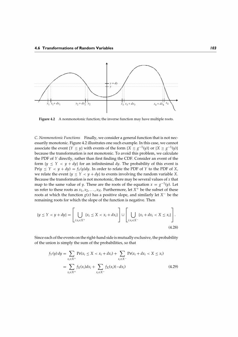
4.6 Transformations of Random Variables 103
x1 x1+ dx1 x2 + dx2 x2 x4 + dx4x4
x3 x3 + dx3
y + dyy
Figure 4.2 A nonmonotonic function; the inverse function may have multiple roots.
C. Nonmonotonic Functions Finally, we consider a general function that is not nec-essarily monotonic. Figure 4.2 illustrates one such example. In this case, we cannotassociate the event {Y ≤ y} with events of the form {X ≤ g−1(y)} or {X ≥ g−1(y)}because the transformation is not monotonic. To avoid this problem, we calculatethe PDF of Y directly, rather than first finding the CDF. Consider an event of theform {y ≤ Y < y + dy} for an infinitesimal dy. The probability of this event isPr(y ≤ Y < y + dy) = fY(y)dy. In order to relate the PDF of Y to the PDF of X,we relate the event {y ≤ Y < y + dy} to events involving the random variable X.Because the transformation is not monotonic, there may be several values of x thatmap to the same value of y. These are the roots of the equation x = g−1(y). Letus refer to these roots as x1, x2, . . . , xN . Furthermore, let X+ be the subset of theseroots at which the function g(x) has a positive slope, and similarly let X− be theremaining roots for which the slope of the function is negative. Then
{y ≤ Y < y + dy} = ⋃
i:xi∈X+{xi ≤ X < xi + dxi}
∪
⋃
i:xi∈X−{xi + dxi < X ≤ xi}
.
(4.28)
Since each of the events on the right-hand side is mutually exclusive, the probabilityof the union is simply the sum of the probabilities, so that
fY(y) dy =∑
xi∈X+Pr(xi ≤ X < xi + dxi) +
∑xi∈X−
Pr(xi + dxi < X ≤ xi)
=∑
xi∈X+fX(xi)dxi +
∑xi∈X−
fX(xi)(−dxi) (4.29)

104 Chapter 4 Operations on a Single Random Variable
Again, invoking absolute value signs to circumvent the need to have two separatesums and dividing by dy, the following result is obtained:
fY(y) =∑
xi
fX(x)∣∣∣∣dxdy
∣∣∣∣∣∣∣∣xi=g−1(y)
. (4.30)
When it is more convenient, the equivalent expression
fY(y) =∑
xi
fX(x)∣∣∣∣dydx
∣∣∣∣ xi=g−1(y)
, (4.31)
can also be used. The following theorem summarizes the general formula fortransformations of random variables.
THEOREM 4.2: Given a random variable X with known PDF, fX(x), and atransformation Y = g(X), the PDF of Y is
fY(y) =∑
xi
fX(x)∣∣∣∣dxdy
∣∣∣∣∣∣∣∣xi=g−1(y)
=∑
xi
fX(x)∣∣∣∣dydx
∣∣∣∣ xi=g−1(y)
, (4.32)
where the xi are the roots of the equation y = g(x). The proof precedes the theorem.
EXAMPLE 4.14: Suppose X is a Gaussian random variable with zeromean and variance σ 2 together with a quadratic transformation, Y = X2.For any positive value of y, y = x2 has two real roots, namely x = ±√
y(for negative values of y, there are no real roots). Application ofEquation 4.32 gives
fY(y) =[
fX(+√y)
2∣∣+√
y∣∣ + fX(−√
y)
2∣∣− √
y∣∣]
u(y) = fX(+√y) + fX(−√
y)2√
yu(y).
For a zero mean Gaussian PDF, fX(x) is an even function so thatfX(+√
y) = fX(−√y). Therefore,
fY(y) = 1√y
fX(√
y)u(y) =√
12πyσ 2 exp
(− y
2σ 2
)u(y).
Hence, Y is a gamma random variable.

4.6 Transformations of Random Variables 105
EXAMPLE 4.15: Suppose the same Gaussian random variable fromthe previous example is passed through a half-wave rectifier which isdescribed by the input-output relationship
y = g(x) ={
x x ≥ 0
0 x ≤ 0.
For x > 0, dy/dx = 1 so that fY(y) = fX(y). However, when x < 0,dy/dx = 0, which will create a problem if we try to insert this directly intoEquation 4.32. To treat this case, we note that the event X < 0 is equiv-alent to the event Y = 0; hence Pr(Y = 0) = Pr(X < 0). Since the inputGaussian PDF is symmetric about zero, Pr(X < 0) = 1/2. Basically, therandom variable Y is a mixed random variable. It has a continuous partover the region y > 0 and a discrete part at y = 0. Using a delta function,we can write the PDF of Y as
fY(y) = 1√2πσ 2
exp
(− y2
2σ 2
)u(y) + 1
2δ(y).
Example 4.15 illustrates how to deal with transformations that are flat oversome interval of nonzero length. In general, suppose the transformation y = g(x)is such that g(x) = yo for any x in the interval x1 ≤ x ≤ x2. Then the PDF ofY will include a discrete component (a delta function) of height Pr(Y = yo) =Pr(x1 ≤ x ≤ x2) at the point y = yo. One often encounters transformations thathave several different flat regions. One such “staircase” function is shown inFigure 4.3. Here, a random variable X that may be continuous will be convertedinto a discrete random variable. The classical example of this is analog-to-digital conversion of signals. Suppose the transformation is of a general staircaseform,
y =
y0 x < x1
yi xi ≤ x < xi+1, i = 1, 2, . . . , N − 1
yN x ≥ xN
. (4.33)
Then Y will be a discrete random variable whose PMF is
P(Y = yi) =
Pr(X < x1) i = 0
Pr(xi ≤ x < xi+1) i = 1, 2, . . . , N − 1
Pr(X ≥ xN) i = N
. (4.34)

106 Chapter 4 Operations on a Single Random Variable
y5
y4
y3
y2
y1
x1 x2 x3 x4 x5
y = g(x)
x
Figure 4.3 A staircase (quantizer) transformation: a continuous random variable will beconverted into a discrete random variable.
EXAMPLE 4.16: Suppose X is an exponential random variable with aPDF fX(x) = exp(−x)u(x) and we form a new random variable Y byrounding X down to the nearest integer. That is,
Y = g(X) = floor(X) = k, k ≤ X < k + 1.
Then, the PMF of Y is
P(Y = k) = Pr(k ≤ X < k + 1) =∫ k+1
ke−xdx = e−k − e−(k+1)
= e−k(1 − 1/e), k = 0, 1, 2, . . . .
Hence, quantization of an exponential random variable produces ageometric random variable.
EXAMPLE 4.17: Let X be a random variable uniformly distributedover (−a/2, a/2). Accordingly, its PDF is of the form
fX(x) = 1a
(u(
x + a2
)− u
(x − a
2
)).
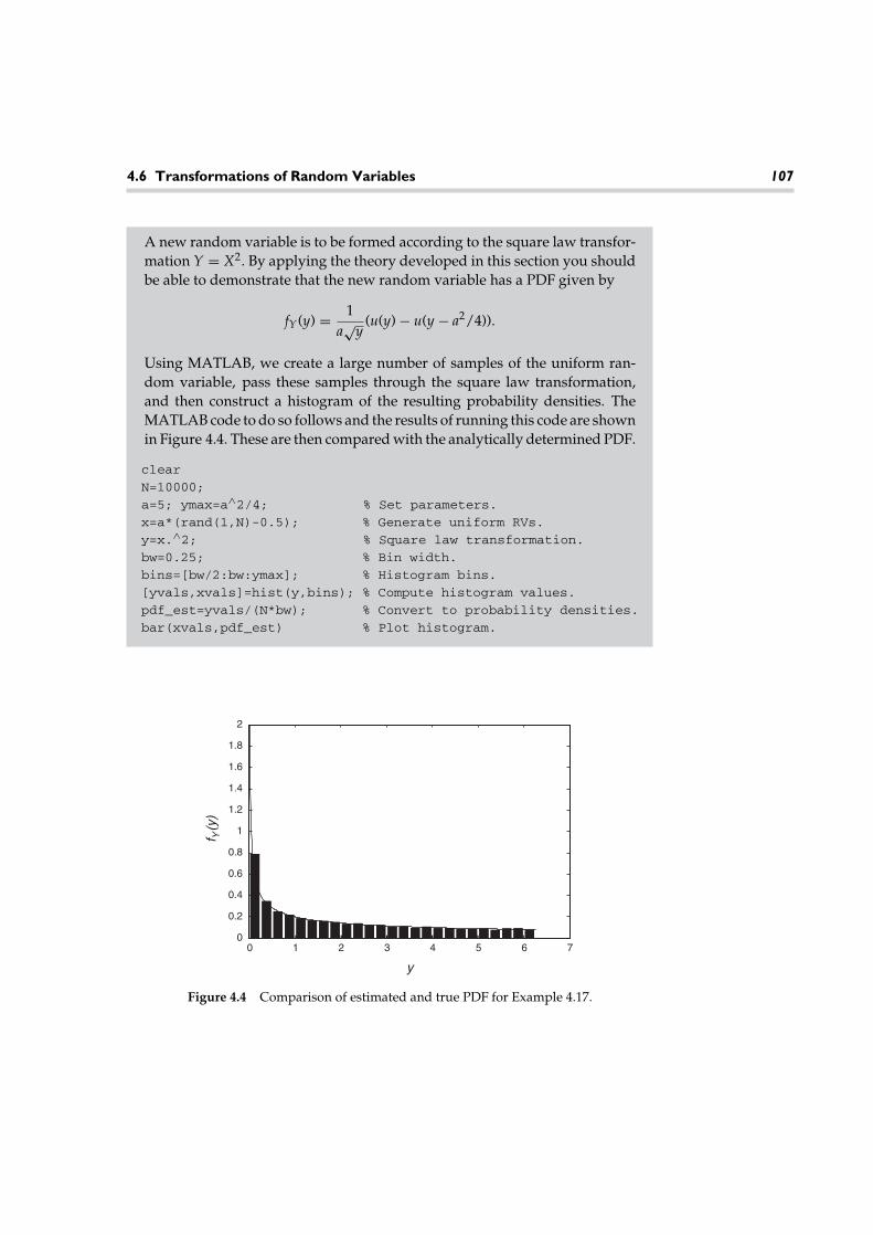
4.6 Transformations of Random Variables 107
A new random variable is to be formed according to the square law transfor-mation Y = X2. By applying the theory developed in this section you shouldbe able to demonstrate that the new random variable has a PDF given by
fY(y) = 1a√
y(u(y) − u(y − a2/4)).
Using MATLAB, we create a large number of samples of the uniform ran-dom variable, pass these samples through the square law transformation,and then construct a histogram of the resulting probability densities. TheMATLAB code to do so follows and the results of running this code are shownin Figure 4.4. These are then compared with the analytically determined PDF.
clear
N=10000;
a=5; ymax=a∧2/4; % Set parameters.
x=a*(rand(1,N)-0.5); % Generate uniform RVs.
y=x.∧2; % Square law transformation.
bw=0.25; % Bin width.
bins=[bw/2:bw:ymax]; % Histogram bins.
[yvals,xvals]=hist(y,bins); % Compute histogram values.
pdf_est=yvals/(N*bw); % Convert to probability densities.
bar(xvals,pdf_est) % Plot histogram.
0 1 2 3 4 5 6 70
0.2
0.4
0.6
0.8
1
1.2
1.4
1.6
1.8
2
y
f Y(y
)
Figure 4.4 Comparison of estimated and true PDF for Example 4.17.

108 Chapter 4 Operations on a Single Random Variable
% Compare true PDF with histogram.
y=[0.01:0.01:ymax];
pdf=1./(a*sqrt(y));
hold on
plot(y,pdf)
xlabel(‘y’); ylabel(‘f_Y(y)’)
hold off
4.7 Characteristic Functions
In this section we introduce the concept of a characteristic function. The charac-teristic function of a random variable is closely related to the Fourier transformof the PDF of that random variable. Thus, the characteristic function providesa sort of “frequency domain” representation of a random variable, although inthis context there is no connection between our frequency variable ω and anyphysical frequency. In studies of deterministic signals, it was found that the use ofFourier transforms greatly simplified many problems, especially those involvingconvolutions. We will see in future chapters the need for performing convolutionoperations on PDFs of random variables and hence frequency domain tools willbecome quite useful. Furthermore, we will find that characteristic functions havemany other uses. For example, the characteristic function is quite useful for find-ing moments of a random variable. In addition to the characteristic function, twoother related functions, namely, the moment-generating function (analogous tothe Laplace transform) and the probability-generating function (analogous to thez-transform), will also be studied in the following sections.
DEFINITION 4.7: The characteristic function of a random variable, X, is given by
�X(ω) = E[e jωX] =∫ ∞
−∞e jωxfX(x) dx. (4.35)
Note the similarity between this integral and the Fourier transform. In most ofthe electrical engineering literature, the Fourier transform of the function fX(x)would be �(−ω). Given this relationship between the PDF and the characteristicfunction, it should be clear that one can get the PDF of a random variable from itscharacteristic function through an inverse Fourier transform operation:
fX(x) = 12π
∫ ∞
−∞e−jωx�X(ω) dω. (4.36)

4.7 Characteristic Functions 109
The characteristic functions associated with various random variables can be easilyfound using tables of commonly used Fourier transforms, but one must be carefulsince the Fourier integral used in Equation 4.35 may be different from the defini-tion used to generate common tables of Fourier transforms. In addition, variousproperties of Fourier transforms can also be used to help calculate characteristicfunctions as shown in the following example.
EXAMPLE 4.18: An exponential random variable has a PDF given byfX(x) = exp(−x)u(x). Its characteristic function is found to be
�X(ω) =∫ ∞
−∞ejωxfX(x) dx =
∫ ∞
0e jωxe−xdx = − e−(1−jω)x
1 − jω
∣∣∣∣∞
0= 1
1 − jω.
This result assumes that ω is a real quantity. Now suppose anotherrandom variable Y has a PDF given by fY(y) = a exp(−ay)u(y). Notethat fY(y) = afX(ay), thus using the scaling property of Fourier trans-forms, the characteristic function associated with the random variableY is given by
�Y(ω) = a1|a|�X
(ω
a
)= 1
1 − jω/a= a
a − jω,
assuming a is a positive constant (which it must be for Y to havea valid PDF). Finally, suppose that Z has a PDF given by fZ(z) =a exp(−a(z − b))u(z − b). Since fZ(z) = fY(z − b), the shifting property ofFourier transforms can be used to help find the characteristic functionassociated with the random variable Z:
�Z(ω) = �Y(ω)e−jωb = ae −jωb
a − jω.
The next example demonstrates that the characteristic function can also be com-puted for discrete random variables. In Section 4.8, the probability-generatingfunction will be introduced and is preferred by some when dealing with discreterandom variables.
EXAMPLE 4.19: A binomial random variable has a PDF that can beexpressed as
fX(x) =n∑
k=0
(nk
)pk(1 − p)n−kδ(x − k).
110 Chapter 4 Operations on a Single Random Variable
Its characteristic function is computed as follows:
�X(ω)=∫ ∞
−∞e jωx
( n∑k=0
(nk
)pk(1−p)n−kδ(x−k)
)dx
=n∑
k=0
(nk
)pk(1−p)n−k
∫ ∞
−∞δ(x−k)e jωxdx=
n∑k=0
(nk
)pk(1−p)n−ke jωk
=n∑
k=0
(nk
)(pejω)k(1−p)n−k = (1−p + pejω)n.
Since the Gaussian random variable plays such an important role in so manystudies, we derive its characteristic function in Example 4.20. We recommend thatthe student commit the result of this example to memory. The techniques usedto arrive at this result are also important and should be carefully studied andunderstood.
EXAMPLE 4.20: For a standard normal random variable, the charac-teristic function can be found as follows:
�X(ω)=∫ ∞
−∞1√2π
e− x22 e jωxdx=
∫ ∞
−∞1√2π
exp
(− (x2−2jωx)
2
)dx.
To evaluate this integral, we complete the square in the exponent.
�X(ω) = exp
(−ω2
2
)∫ ∞
−∞1√2π
exp
(− (x2 − 2jωx − ω2)
2
)dx
= exp
(−ω2
2
)∫ ∞
−∞1√2π
exp
(− (x − jω)2
2
)dx
The integrand in this expression looks like the properly normalizedPDF of a Gaussian random variable, and since the integral is over allvalues of x, the integral must be unity. However, close examinationof the integrand reveals that the “mean” of this Gaussian integrand iscomplex. It is left to the student to rigorously verify that this integral stillevaluates to unity even though the integrand is not truly a Gaussian PDF

4.7 Characteristic Functions 111
(since it is a complex function and hence not a PDF at all). The resultingcharacteristic function is then
�X(ω) = exp
(−ω2
2
).
For a Gaussian random variable whose mean is not zero or whose stan-dard deviation is not unity (or both), the shifting and scaling propertiesof Fourier transforms can be used to show that
fX(x) = 1√2πσ 2
e− (x−µ)2
2σ2 ↔ �X(ω) = exp
(jµω − ω2σ 2
2
).
THEOREM 4.3: For any random variable whose characteristic function is differ-entiable at ω = 0,
E[X] = −jd
dω�X(ω)
∣∣∣∣ω=0
. (4.37)
PROOF: The proof follows directly from the fact that the expectation and differ-entiation operations are both linear and consequently the order of these operationscan be exchanged.
ddω
�X(ω) = ddω
E[e jωX
]= E
[d
dωe jωX
]= E
[jXe jωX
]= jE
[Xe jωX
].
Multiplying both sides by −j and evaluating at ω = 0 produces the desiredresult. �
Theorem 4.3 demonstrates a very powerful use of the characteristic function.Once the characteristic function of a random variable has been found, it is gen-erally a very straightforward thing to produce the mean of the random variable.Furthermore, by taking the kth derivative of the characteristic function and evaluat-ing at ω = 0, an expression proportional to the kth moment of the random variableis produced. In particular,
E[Xk] = (−j)k dk
dωk�X(ω)
∣∣∣∣ω=0
. (4.38)
Hence, the characteristic function represents a convenient tool to easily determinethe moments of a random variable.

112 Chapter 4 Operations on a Single Random Variable
EXAMPLE 4.21: Consider the exponential random variable ofExample 4.18 where fY(y) = a exp(−ay)u(y). The characteristic functionwas found to be
�Y(ω) = aa − jω
.
The derivative of the characteristic function is
ddω
�Y(ω) = ja(a − jω)2 ,
and thus the first moment of Y is
E[Y] = −jd
dω�Y(ω)
∣∣∣∣ω=0
= a(a − jω)2
∣∣∣∣ω=0
= 1a
.
For this example, it is not difficult to show that the kth derivative of thecharacteristic function is
dk
dωk�Y(ω) = jkk!a
(a − jω)k+1,
and from this, the kth moment of the random variable is found to be
E[Yk] = (−j)k dk
dωk�Y(ω)
∣∣∣∣ω=0
= k!a(a − jω)k+1
∣∣∣∣ω=0
= k!ak
.
For random variables that have a more complicated characteristic function,evaluating the kth derivative in general may not be an easy task. However,Equation 4.38 only calls for the kth derivative evaluated at a single point (ω = 0),which can be extracted from the Taylor series expansion of the characteristic func-tion. To see this, note that from Taylor’s Theorem, the characteristic function canbe expanded in a power series as
�X(ω) =∞∑
k=0
1k!
(dk
dωk�X(ω)
∣∣∣∣ω=0
)ωk. (4.39)
If one can obtain a power series expansion of the characteristic function, thenthe required derivatives are proportional to the coefficients of the power series.Specifically, suppose an expansion of the form
�X(ω) =∞∑
k=0
φkωk (4.40)

4.7 Characteristic Functions 113
is obtained. Then the derivatives of the characteristic function are given by
dk
dωk�X(ω)
∣∣∣∣ω=0
= k!φk. (4.41)
The moments of the random variable are then given by
E[Xk] = (−j)kk!φk. (4.42)
This procedure is illustrated using a Gaussian random variable in the next example.
EXAMPLE 4.22: Consider a Gaussian random variable with a mean ofµ = 0 and variance σ 2. Using the result of Example 4.20, the character-istic function is �X(ω) = exp(−ω2σ 2/2). Using the well-known Taylorseries expansion of the exponential function, the characteristic functionis expressed as
�X(ω) =∞∑
n=0
(−ω2σ 2/2)n
n! =∞∑
n=0
(−1)nσ 2n
2nn! ω2n.
The coefficients of the general power series as expressed in Equation 4.40are given by
φk =
jk(σ/√
2)k
(k/2)! k even
0 k odd.
Hence the moments of the zero-mean Gaussian random variable are
E[Xk] =
k!(k/2)!
(σ√
2
)k
k even
0 k odd.
As expected, E[X0] = 1, E[X] = 0 (since it was specified that µ = 0), andE[X2] = σ 2 (since in the case of zero-mean variables, the second momentand variance are one and the same). Now, we also see that E[X3] = 0(i.e., all odd moments are equal to zero), E[X4] = 3σ 4, E[X6] = 15σ 6,and so on. We can also conclude from this that for Gaussian randomvariables, the coefficient of skewness is cs = 0, while the coefficient ofkurtosis is ck = 3.
In many cases of interest, the characteristic function has an exponential form.The Gaussian random variable is a typical example. In such cases, it is convenientto deal with the natural logarithm of the characteristic function.

114 Chapter 4 Operations on a Single Random Variable
DEFINITION 4.8: In general, we can write a series expansion of ln[�X(ω)] as
ln[�X(ω)] =∞∑
n=1
λn(jω)n
n! . (4.43)
where the coefficients, λn, are called the cumulants and are given as
λn = dn
d(jω)n {ln[�X(ω)]}∣∣∣∣ω=0
, n = 1, 2, 3, . . . . (4.44)
The cumulants are related to the moments of the random variable. By takingthe derivatives specified in Equation 4.44 we obtain
λ1 = µX , (4.45)
λ2 = E[X2] − µ2X = σ 2
X , (4.46)
λ3 = E[X3] − 3µXE[X2] + 2µ3X = E[(X − µX)3]. (4.47)
Thus, λ1 is the mean, λ2 is the second central moment (or the variance), and λ3is the third central moment. However, higher order cumulants are not as simplyrelated to the central moments.
4.8 Probability Generating Functions
In the world of signal analysis, we often use Fourier transforms to describecontinuous time signals, but when we deal with discrete time signals, it iscommon to use a z-transform instead. In the same way, the characteristic func-tion is a useful tool for working with continuous random variables, but whendiscrete random variables are concerned, it is often more convenient to use adevice similar to the z-transform which is known as the probability generatingfunction.
DEFINITION 4.9: For a discrete random variable with a probability mass func-tion, PX(k), defined on the nonnegative integers1, k = 0, 1, 2, . . . , the probability
1Note that this definition assumes that the discrete random variable, X, is defined onnonnegative integer values, k. One could also define a probability generating function basedon a bilateral z-transform that would allow for random variables that can take on negativeinteger values as well. However, since this is less common, we do not consider it furtherhere.

4.8 Probability Generating Functions 115
generating function, HX(z), is defined as
HX(z) =∞∑
k=0
PX(k)zk. (4.48)
Note the similarity between the probability generating function and the unilateralz-transform of the probability mass function.
Since the PMF is seen as the coefficients of the Taylor series expansion of HX(z),it should be apparent that the PMF can be obtained from the probability generatingfunction through
PX(k) = 1k!
dk
dzkHX(z)
∣∣∣∣z=0
. (4.49)
The derivatives of the probability generating function evaluated at zero returnthe PMF and not the moments as with the characteristic function. However, themoments of the random variable can be obtained from the derivatives of theprobability generating function at z = 1.
THEOREM 4.4: The mean of a discrete random variable can be found from itsprobability generating function according to
E[X] = ddz
HX(z)∣∣∣∣z=1
. (4.50)
Furthermore, the higher order derivatives of the probability generating functionevaluated at z = 1 lead to quantities known as the factorial moments,
hk = dk
dzkHX(z)
∣∣∣∣z=1
= E[X(X − 1)(X − 2) · · · (X − k + 1)]. (4.51)
PROOF: The result follows directly from differentiating Equation 4.48. The detailsare left to the reader. �
It is a little unfortunate that these derivatives don’t produce the momentsdirectly, but the moments can be calculated from the factorial moments. Forexample,
h2 = E[X(X − 1)] = E[X2] − E[X] = E[X2] − h1,
⇒ E[X2] = h2 + h1. (4.52)
Hence, the second moment is simply the sum of the first two factorial moments. Ifwe were interested in the variance as well, we would obtain
σ 2X = E[X2] − µ2
X = h2 + h1 − h21. (4.53)

116 Chapter 4 Operations on a Single Random Variable
EXAMPLE 4.23: Consider the binomial random variable of Example 4.4whose PMF is
PX(k) =(
nk
)pk(1 − p)n−k, k = 0, 1, 2, . . . , n.
The corresponding probability generating function is
HX(z)=n∑
k=0
(nk
)pk(1−p)n−kzk =
n∑k=0
(nk
)(pz)k(1−p)n−k = (1−p+pz)n.
Evaluating the first few derivatives at z = 1 produces
h1 = ddz
HX(z)∣∣∣∣z=1
= np(1 − p + pz)n−1∣∣∣∣z=1
= np,
h2 = d2
dz2 HX(z)∣∣∣∣z=1
= n(n − 1)p2(1 − p + pz)n−2∣∣∣∣z=1
= n(n − 1)p2.
From these factorial moments, we calculate the mean, second moment,and variance of a binomial random variable as
µX = h1 = np, E[X2] = h1 + h2 = (np)2 + np(1 − p), σ 2X = h2 + h1 − h2
1
= np(1 − p).
In order to gain an appreciation for the power of these “frequency domain” tools,compare the amount of work used to calculate the mean and variance of the bino-mial random variable using the probability generating function in Example 4.23with the direct method used in Example 4.4.
As was the case with the characteristic function, we can compute higher orderfactorial moments without having to take many derivatives by expanding the prob-ability generating function into a Taylor series. In this case, the Taylor series must

4.9 Moment Generating Functions 117
be about the point z = 1.
HX(z) =∞∑
k=0
1k!
(dk
dzkHX(z)
∣∣∣∣z=1
)(z − 1)k =
∞∑k=0
1k!hk(z − 1)k (4.54)
Once this series is obtained, one can easily identify all of the factorial moments.This is illustrated using a geometric random variable in Example 4.24.
EXAMPLE 4.24: A geometric random variable has a PMF given byPX(k) = (1 − p)pk, k = 0, 1, 2, . . . . The probability generating function isfound to be
HX(z) =∞∑
k=0
(1 − p)(pz)k = 1 − p1 − pz
.
In order to facilitate forming a Taylor series expansion of this func-tion about the point z = 1, it is written explicitly as a function of z − 1.From there, the power series expansion is fairly simple:
HX(z) = 1 − p1 − p − p(z − 1)
= 1
1 − p1 − p
(z − 1)=
∞∑k=0
(p
1 − p
)k
(z − 1)k.
Comparing the coefficients of this series with the coefficients given inEquation 4.54 leads to immediate identification of the factorial moments,
hk = k!pk
(1 − p)k.
4.9 Moment Generating Functions
In many problems, the random quantities we are studying are often inherentlynonnegative. Examples include the frequency of a random signal, the time betweenarrivals of successive customers in a queueing system, or the number of pointsscored by your favorite football team. The resulting PDFs of these quantities arenaturally one-sided. For such one-sided waveforms, it is common to use Laplacetransforms as a frequency domain tool. The moment generating function is theequivalent tool for studying random variables.

118 Chapter 4 Operations on a Single Random Variable
DEFINITION 4.10: The moment generating function, MX(u), of a nonnegative2
random variable, X, is
MX(u) = E[euX] =∫ ∞
0fX(x)eux dx. (4.55)
Note the similarity between the moment generating function and the Laplacetransform of the PDF.
The PDF can in principle be retrieved from the moment generating functionthrough an operation similar to an inverse Laplace transform,
fX(x) = 12π j
∫ c+j∞
c−j∞MX(u)e−uxdu. (4.56)
Because the sign in the exponential term in the integral in Equation 4.55 is theopposite of the traditional Laplace transform, the contour of integration (the so-called Bromwich contour) in the integral specified in Equation 4.56 must now beplaced to the left of all poles of the moment generating function. As with thecharacteristic function, the moments of the random variable can be found from thederivatives of the moment generating function (hence, its name) according to
E[Xk] = dk
dukMX(u)
∣∣∣∣u=0
. (4.57)
It is also noted that if the moment generating function is expanded in a power seriesof the form
MX(u) =∞∑
k=0
mkuk, (4.58)
then the moments of the random variable are given by E[Xk] = k!mk.
EXAMPLE 4.25: Consider an Erlang random variable with a PDF of theform
fX(x) = xn−1 exp(−x)u(x)(n − 1)! .
2One may also define a moment generating function for random variables that are notnecessarily nonnegative. In that case, a two-sided Laplace transform would be appropriate.This would be identical to the characteristic function with the association u = jω.
4.10 Evaluating Tail Probabilities 119
The moment generating function is calculated according to
MX(u) =∫ ∞
0fX(x)euxdx =
∫ ∞
0
xn−1 exp(−(1 − u)x)(n − 1)! dx.
To evaluate this function, we note that the integral looks like theLaplace transform of the function xn−1/(n − 1)! evaluated at s = 1 − u.Using standard tables of Laplace transforms (or using integration byparts several times), we get
MX(u) = 1(1 − u)n .
The first two moments are then found as follows:
E[X] = ddu
(1 − u)−n∣∣∣∣u=0
= n(1 − u)−(n+1)∣∣∣∣u=0
= n,
E[X2] = d2
du2 (1 − u)−n∣∣∣∣u=0
= n(n + 1)(1 − u)−(n+2)∣∣∣∣u=0
= n(n + 1).
From this, we could also infer that the variance is σ 2X = n(n+1)−n2 = n.
If we wanted a general expression for the kth moment, it is not hard tosee that
E[Xk] = dk
duk(1 − u)−n
∣∣∣∣u=0
= n(n + 1) · · · (n + k − 1) = (n + k − 1)!(n − 1)! .
4.10 Evaluating Tail Probabilities
A common problem encountered in a variety of applications is the need to computethe probability that a random variable exceeds a threshold, Pr(X > xo). Alterna-tively, we might want to know, Pr(|X−µx| > xo). These quantities are referred to astail probabilities. That is, we are asking, what is the probability that the random vari-able takes on a value that is in the tail of the distribution? While this can be founddirectly from the CDF of the random variable, quite often the CDF may be diffi-cult or even impossible to find. In those cases, one can always resort to numericalintegration of the PDF. However, this involves a numerical integration over a semi-infinite region, which in some cases may be problematic. Then, too, in some situa-tions we might not even have the PDF of the random variable, but rather the randomvariable may be described in some other fashion. For example, we may know only

120 Chapter 4 Operations on a Single Random Variable
the mean or the mean and variance, or the random variable may be described byone of the frequency domain functions described in the previous sections.
Obviously, if we are given only partial information about the random variable,we would not expect to be able to perfectly evaluate the tail probabilities, butwe can obtain bounds on these probabilities. In this section, we present severaltechniques for obtaining various bounds on tail probabilities based on differentinformation about the random variable. We then conclude the section by showinghow to exactly evaluate the tail probabilities directly from one of the frequencydomain descriptions of the random variables.
THEOREM 4.5 (Markov’s Inequality): Suppose that X is a nonnegative randomvariable (i.e., one whose PDF is nonzero only over the range [0, ∞)). Then
Pr(X ≥ xo) ≤ E[X]xo
. (4.59)
PROOF: For nonnegative random variables, the expected value is
E[X] =∫ ∞
0xfX(x) dx =
∫ xo
0xfX(x) dx +
∫ ∞
xo
xfX(x) dx ≥∫ ∞
xo
xfX(x) dx
≥ xo
∫ ∞
xo
fX(x) dx. (4.60)
Dividing both sides by xo gives the desired result.Markov’s inequality provides a bound on the tail probability. The bound
requires only knowledge of the mean of the random variable. Because the bounduses such limited information, it has the potential of being very loose. In fact, ifxo < E[X], then the Markov inequality states that Pr(X ≥ xo) is bounded by anumber that is greater than 1. While this is true, in this case the Markov inequalitygives us no useful information. Even in less extreme cases, the result can still bevery loose as shown by the next example. �
EXAMPLE 4.26: Suppose the average life span of a person was 75years. The probability of a human living to be 110 years would thenbe bounded by
Pr(X ≥ 110) ≤ 75110
= 0. 6818.
Of course, we know that in fact very few people live to be 110 years old,and hence this bound is almost useless to us.

4.10 Evaluating Tail Probabilities 121
If we know more about the random variable than just its mean, we can obtaina more precise estimate of its tail probability. In Example 4.26, we know that thebound given by the Markov inequality is ridiculously loose because we knowsomething about the variability of the human life span. The next result allows usto use the variance as well as the mean of a random variable to form a differentbound on the tail probability.
THEOREM 4.6 (Chebyshev’s Inequality): Suppose that X is a random variablewith mean µX and variance σ 2
X . The probability that the random variable takes ona value that is removed from the mean by more than xo is given by
Pr(|X − µX| ≥ xo) ≤ σ 2X
x2o
. (4.61)
PROOF: Chebyshev’s inequality is a direct result of Markov’s inequality. First,note that the event {|X − µX| ≥ xo} is equivalent to the event {(X − µX)2 ≥ x2
o}.Applying Markov’s inequality to the later event results in
Pr((X − µX)2 ≥ x2o ) ≤ E[(X − µX)2]
x2o
= σ 2X
x2o
. (4.62)
Note that Chebyshev’s inequality gives a bound on the two-sided tail probabil-ity, whereas the Markov inequality applies to the one-sided tail probability. Also,the Chebyshev inequality can be applied to any random variable, not just to thosethat are nonnegative. �
EXAMPLE 4.27: Continuing the previous example, suppose that inaddition to a mean of 75 years, the human life span had a standarddeviation of 5 years. In this case,
Pr(X ≥ 110) ≤ Pr(X ≥ 110) + Pr(X ≤ 40) = Pr(|X − 75| ≥ 35).
Now the Chebyshev inequality can be applied to give
Pr(|X − 75| ≥ 35) ≤(
535
)2
= 149
.
While this result may still be quite loose, by using the extra piece ofinformation provided by the variance, a better bound is obtained.

122 Chapter 4 Operations on a Single Random Variable
u(x–xo)
xxo
exp(s(x–xo))
Figure 4.5 The unit step function and an exponential upper bound.
THEOREM 4.7 (Chernoff Bound): Suppose X is a random variable whosemoment generating function is MX(s). Then
Pr(X ≥ xo) ≤ mins≥0
e−sxo MX(s). (4.63)
PROOF: First, note that
Pr(X ≥ xo) =∫ ∞
xo
fX(x) dx =∫ ∞
−∞fX(x)u(x − xo) dx. (4.64)
Next, upper bound the unit step function in the integrand by an exponential func-tion of the form u(x − xo) ≤ exp(s(x − xo)). This bound is illustrated in Figure 4.5.Note that the bound is valid for any real s ≥ 0. The tail probability is then upperbounded by
Pr(X ≥ xo) ≤ e−sxo
∫ ∞
−∞fX(x)esxdx = e−sxo MX(s). (4.65)
Since this bound is valid for any s ≥ 0, it can be tightened by finding the valueof s that minimizes the right-hand side. In this expression, a two-sided Laplacetransform must be used to obtain the moment generating function if the randomvariable is not nonnegative (see footnote 2 associated with Definition 4.10). �
EXAMPLE 4.28: Consider a standard normal random variable whosemoment generating function is given by MX(u) = exp(u2/2) (see resultof Example 4.20, where the characteristic function is found, and replaceω with −ju). The tail probability, Pr(X ≥ xo), in this case is simply the

4.10 Evaluating Tail Probabilities 123
Q-function, Q(xo). According to Equation 4.65, this tail probability canbe bounded by
Q(xo) ≤ exp
(−uxo + u2
2
)
for any u ≥ 0. Minimizing with respect to u, we get
ddu
exp
(−uxo + u2
2
)= (−xo + u) exp
(−uxo + u2
2
)= 0 ⇒ u = xo.
Hence, the Chernoff bound on the tail probability for a standardnormal random variable is
Q(xo) ≤ exp
(−x2
o
2
).
The result of this example provides a convenient upper bound on theQ-function.
Evaluating the Chernoff bound requires knowledge of the moment generat-ing function of the random variable. This information is sufficient to calculate thetail probability exactly since, in theory, one can obtain the PDF from the momentgenerating function, and from there the exact tail probability can be obtained.However, in cases where the moment generating function is of a complicated ana-lytical form, determining the PDF may be exceedingly difficult. Indeed, in somecases, it may not be possible to express the tail probability in closed form (as withthe Gaussian random variable). In these cases, the Chernoff bound will often pro-vide an analytically tractable expression that can give a crude bound on the tailprobability. If a precise expression for the tail probability is required, the result ofTheorem 4.8 will show how this can be obtained directly from the momentgenerating function (without having to explicitly find the PDF).
THEOREM 4.8: For a random variable, X, with a moment generating function,MX(u), an exact expression for the tail probability, Pr(X ≥ xo), is given by
Pr(X ≥ xo) = 12π j
∫ c+j∞
c−j∞MX(u)
ue−uxo du, (4.66)
where the contour of integration is to the right of the origin but to the left of allsingularities of the moment generating function in the right half-plane.

124 Chapter 4 Operations on a Single Random Variable
PROOF: The right tail probability is given in general by
Pr(X ≥ xo) =∫ ∞
xo
fX(x) dx. (4.67)
Then, replace the PDF in this integral with an inverse transform of the momentgenerating function as specified in Equation 4.56.
Pr(X ≥ xo) =∫ ∞
xo
12π j
∫ c+j∞
c−j∞MX(u)e−uxdudx
= 12π j
∫ c+j∞
c−j∞MX(u)
∫ ∞
xo
e−uxdxdu (4.68)
Evaluating the inner integral results in
Pr(X ≥ xo) = 12π j
∫ c+j∞
c−j∞MX(u)
ue−uxo du, for Re[u] > 0. (4.69)
The integral specified in Equation 4.66 can be evaluated numerically or, whenconvenient to do so, it can also be evaluated by computing the appropriateresidues3. For xo > 0, the contour of integration can be closed to the right. Theresulting closed contour will encompass all the singularities of the moment gen-erating function in the right half-plane. According to Cauchy’s residue theorem,the value of the integral will then be −2π j times the sum of the residues of all thesingularities encompassed by the contour. Hence,
Pr(X ≥ xo) =∑
right half-plane
Residues{
MX(u)u
e−uxo
}. (4.70)
If a precise evaluation of the tail probability is not necessary, several approx-imations to the integral in Equation 4.66 are available. Perhaps the simplest andmost useful is known as the saddle point approximation. To develop the saddle pointapproximation, define ψ(u) = ln(MX(u)) and
λ(u) = ln(
MX(u)u
e−uxo
)= ψ(u) − uxo − ln(u). (4.71)
Furthermore, consider a Taylor series expansion of the function λ(u) about somepoint u = uo,
λ(u) = λ(uo) + λ′(uo)(u − uo) + 12λ′′(uo)(u − uo)2 + · · · . (4.72)
3The remainder of this section assumes a familiarity with the concepts of contour inte-gration and residue calculus. For those unfamiliar with these topics, the remainder of thissection can be skipped without any loss in continuity.

4.10 Evaluating Tail Probabilities 125
In particular, if uo is chosen so that λ′(uo) = 0, then near the point u = uo, theintegrand in Equation 4.66 behaves approximately like
MX(u)u
e−uxo = eλ(u) ≈ exp(λ(uo)) exp(
12λ′′(uo)(u − uo)2
). (4.73)
In general, the point u = uo will be a minima of the integrand as viewed alongthe real axis. This follows from the fact that the integrand is a concave function ofu. A useful property of complex (analytic) functions tells us that if the function hasa minima at some point uo as u passes through it in one direction, the function willalso have a maxima as u passes through the same point in the orthogonal direction.Such a point is called a “saddle point” since the shape of the function resembles asaddle near that point. If the contour of integration is selected to pass through thesaddle point, the integrand will reach a local maximum at the saddle point. As justseen in Equation 4.73, the integrand also has a Gaussian behavior at and aroundthe saddle point. Hence, using the approximation of Equation 4.73 and runningthe contour of integration through the saddle point so that u = uo + jω along theintegration contour, the tail probability is approximated by
Pr(X ≥ xo) ≈ exp(λ(uo))2π j
∫ uo+j∞
uo−j∞exp
(12λ′′(uo)(u − uo)2
)du
= exp(λ(uo))2π
∫ ∞
−∞exp
(−1
2λ′′(uo)ω2
)dω
= exp(λ(uo))√2πλ′′(uo)
= MX(uo) exp(−uoxo)
uo√
2πλ′′(uo). (4.74)
The third step is accomplished using the normalization integral for Gaussian PDFs.The saddle point approximation is usually quite accurate provided that
xo � E[X]. That is, the farther we go out into the tail of the distribution, the bet-ter the approximation. If it is required to calculate Pr(X ≥ xo) for xo < E[X], it isusually better to calculate the left tail probability, in which case the saddle pointapproximation is
Pr(X ≥ xo) ≈ −MX(uo) exp(−uoxo)
uo√
2πλ′′(uo), (4.75)
where in this case the saddle point, uo, must be negative. �

126 Chapter 4 Operations on a Single Random Variable
EXAMPLE 4.29: In this example, we will form the saddle point approx-imation to the Q-function that is the right tail probability for a stan-dard normal random variable. The corresponding moment generatingfunction is MX(u) = exp(u2/2). To find the saddle point, we note that
λ(u) = u2
2− ln(u) − uxo.
We will need the first two derivatives of this function:
λ′(u) = u − 1u
− xo, λ′′(u) = 1 + 1u2 .
The saddle point is the solution to λ′(uo) = 0 that results in a quadraticequation whose roots are
uo = xo ± √x2
o + 42
.
When calculating the right tail probability, the saddle point must be tothe right of the imaginary axis, hence the positive root must be used:
uo = xo + √x2
o + 42
.
The saddle point approximation then becomes
Q(xo) ≈ Mx(uo) exp(−uoxo)
uo√
2πλ′′(uo)=
exp
(−u2
o
2− uoxo
)
√2π (1 + u2
o ).
The exact value of the Q-function and the saddle point approximationare compared in Figure 4.6. As long as xo is not close to zero, thisapproximation is quite accurate.
4.11 Engineering Application: ScalarQuantization
In many applications, it is convenient to convert a signal that is analog in natureto a digital one. This is typically done in three steps. First, the signal is sampled,

4.11 Engineering Application: Scalar Quantization 127
0 0.5 1 1.5 2 2.5 3 3.5 4
100
10−1
10−2
10−3
10−4
10−5
Pr(
X>
x o)
xo
Q-functionSaddle point ± approximation
Figure 4.6 The Q-function and its saddle point approximation.
which converts the signal from continuous time to discrete time. Then samples ofthe signal are quantized. This second action converts the signal from one with acontinuous amplitude to one whose amplitude can only take on discrete values.Once the signal is converted to discrete time/discrete amplitude, the signal can theneasily be represented by a sequence of bits. In this third step, each discrete ampli-tude level is represented by a binary code word. While the first step (sampling)and the third step (encoding) are invertible, the second step (quantization) is not.That is, we can perfectly recover the analog signal from its discrete time samples(provided the samples are taken at a rate above the Nyquist rate), and the discreteamplitude levels can easily be recovered from the code words that represent them(provided a lossless source code is used). However, the act of quantization causesdistortion of the signal that cannot be undone. Given the discrete amplitude of asample, it is not possible to determine the exact value of the original (continuousamplitude) sample. For this reason, careful attention is paid to the quantizationprocess to minimize the amount of distortion.
In order to determine efficient ways to quantize signals, we must first quantifythis concept of signal distortion. Suppose a signal is sampled and we focus attentionon one of those samples. Let the random variable X represent the value of thatsample, which in general will draw from a continuous sample space. Now suppose

128 Chapter 4 Operations on a Single Random Variable
that sample is quantized (using some quantization function q(x)) to form a new(discrete) random variable Y = q(X). The difference between the original samplevalue and its quantized value, X − q(X), is the error caused by the quantizer, orthe quantizer noise. It is common to measure signal distortion as the mean squaredquantizer error,
d = E[(X − q(X))2] =∫ ∞
−∞(x − q(x))2fX(x) dx. (4.76)
We will see Chapter 10 in the text, that the mean square value of a signal has thephysical interpretation of the signal’s power. Thus, the quantity d can be interpretedas the quantization noise power. Often the fidelity of a quantized signal is measuredin terms of the ratio of the original signal power, E[X2], to the quantization noisepower. This is referred to as the signal–to–quantization noise power ratio (SQNR):
SQNR = E[X2]E[(X − q(X))2] . (4.77)
The goal of the quantizer design is to choose a quantization function that minimizesthe distortion, d. Normally, the quantizer maps the sample space of X into one ofM = 2n levels. Then each quantization level can be represented by a unique n-bitcode word. We refer to this as an n-bit quantizer. As indicated in Equation 4.76,the expected value is with respect to the PDF of X. Hence, the function q(x) thatminimizes the distortion will depend on the distribution of X.
To start with, consider a random variable X that is uniformly distributed overthe interval (−a/2, a/2). Since the sample X is equally likely to fall anywhere in theregion, it would make sense for the quantizer to divide that region into M equallyspaced subintervals of width = a/M. For each subinterval, the quantization level(i.e., the value of q(x) for that subinterval) should be chosen as the midpoint of thesubinterval. This is referred to as a uniform quantizer. A 3-bit uniform quantizeris illustrated in Figure 4.7. For example, if X ∈ (0, a/8), then q(X) = a/16. Tomeasure the distortion for this signal together with the uniform quantizer, assumethat the signal falls within one of the quantization intervals, given that quantizationinterval, and then use the theorem of total probability:
d = E[(X − q(X))2] =8∑
k=1
E[(X − q(X))2|X ∈ Xk] Pr(X ∈ Xk), (4.78)
where Xk refers to the kth quantization interval. Consider, for example, X5 =(0, a/8), so that
E[(X − q(X))2|X ∈ X5] = E[X − a/16)2|X ∈ (0, a/8)]. (4.79)

4.11 Engineering Application: Scalar Quantization 129
q(x)
x
a/2
a/4
–a/2 –a/4
a/4 a/2
–a/2
–a/4
Figure 4.7 A 3-bit uniform quantizer on the interval (−a/2, a/2)
To calculate this conditional expected value requires the conditional PDF of X.From Equation 3.41 this is
fX(x|X ∈ (0, a/8)) = fX(x)Pr(X ∈ (0, a/8))
= 1/a1/8
= 8a
, x ∈ (0, a/8). (4.80)
Not surprisingly, conditioned on X ∈ (0, a/8), X is uniformly distributed over(0, a/8). The conditional expected value is then
E[(X − a/16)2|X ∈ (0, a/8)] = 8a
∫ a/8
0(x − a/16)2dx = a2
768. (4.81)
Due to the symmetry of the uniform distribution, this conditional distortion isthe same regardless of what quantization interval the signal falls in. Hence,Equation 4.81 is also the unconditional distortion. Note that the power of theoriginal signal is
E[X2] = 1a
∫ a/2
−a/2x2dx = a2
12. (4.82)
The resulting SQNR is then
SQNR = E[X2]d
= a2/12a2/768
= 64 = 18. 06 dB. (4.83)
The preceding result for the 3-bit uniform quantizer can be generalized toany uniform quantizer. In general, for an n-bit uniform quantizer, there willbe M = 2n quantization intervals of width = a/M. Consider the quantization

130 Chapter 4 Operations on a Single Random Variable
interval (0, ) and suppose that quantization level for that interval is chosen to bethe midpoint, /2. Then the distortion for that interval (and hence the distortionfor the quantizer) is
E[(X − q(X))2|X ∈ (0, )] = 1
∫
0(x − /2)2dx = 2/12. (4.84)
The SQNR for an n-bit uniform quantizer with a uniformly distributed input is
SQNR = E[X2]d
= a2/12 2/12
= M2 = 22n or SQNR(dB) = 2nlog10(2) = 6. 02n dB.
(4.85)
This is the so-called 6 dB rule whereby the SQNR is increased by approximately 6 dBfor each extra bit added to the quantizer. For example, in wireline digital telephony,8-bit quantization is used that would result in an SQNR of approximately 48 dB.
The previous results assumed that the input to the quantizer followed a uniformprobability distribution. This is rarely the case. Speech signals, for example, arecommonly modeled using a Laplace (two-sided exponential) distribution. For suchsignals, small sample values are much more frequent than larger values. In such asituation, it would make sense to use finer resolution (i.e., narrower quantizationintervals) for the more frequent smaller amplitudes in order to keep the distortionminimized in those regions, at the cost of more distortion in the less frequent largeramplitude regions.
Given that an n-bit quantizer is to be used, the design of an optimum quantizerinvolves two separate problems. First, the ranges for each quantization intervalmust be specified; then the quantization level for each interval must be chosen. Thefollowing theorem specifies how each of these two tasks should be accomplished.
THEOREM 4.9: A random variable X with PDF fX(x) is to be quantized with anM-level quantizer that produces a discrete random variable Y according to
y = q(x) = yi, for xi−1 < x < xi, i = 1, 2, . . . , M, (4.86)
where it is assumed that the lower limit of the first quantization interval is x0 = −∞and the upper limit of the last quantization interval is xM = ∞. The (mean-squared)distortion is minimized by choosing the quantization intervals (i.e., the xi) and thequantization levels (i.e., the yi) according to
(i) yi = E[X|xi−1 < X < xi], i = 1, 2, . . . , M, (the conditional mean criterion),
(4.87)
(ii) xi = yi + yi+1
2, i = 1, 2, . . . , M − 1 (the midpoint criterion). (4.88)

4.11 Engineering Application: Scalar Quantization 131
These two criteria provide a system of 2M − 1 equations with which to solvefor the 2M − 1 quantities (x1, x2, . . . , xM−1, y1, y2, . . . , yM) that specify the optimumM-level quantizer.
PROOF: The distortion is given by
d =M∑
i=1
∫ xi
xi−1
(x − yi)2fX(x) dx. (4.89)
To minimize d with respect to yj,
∂d∂yj
= −2∫ xi
xi−1
(x − yi)fX(x) dx = 0. (4.90)
Solving for yj in this equation establishes the conditional mean criterion. Similarly,differentiating with respect to xj gives
∂d∂xj
= (xj − yj)2fX(xj) − (xj − yj+1)2fX(xj) = 0. (4.91)
Solving for xj produces the midpoint criterion. �
EXAMPLE 4.30: Using the criteria set forth in Theorem 4.9, an idealnonuniform 2-bit quantizer will be designed for a signal whose sampleshave a Laplace distribution, fX(x) = (1/2) exp(−|x|). A 2-bit quantizerwill have four quantization levels, {y1, y2, y3, y4}, and four correspond-ing quantization intervals that can be specified by three boundarypoints, {x1, x2, x3}. The generic form of the 2-bit quantizer is illustratedin Figure 4.8. Due to the symmetry of the Laplace distribution, it seemsreasonable to expect that the quantizer should have a negative sym-metry about the y-axis. That is, x1 = −x3, x2 = 0, y1 = −y4, andy2 = −y3. Hence, it is sufficient to determine just three unknowns, suchas {x3, y3, y4}. The rest can be inferred from the symmetry. Applicationof the conditional mean criterion and the midpoint criterion leads to thefollowing set of three equations:
y3 = E[X|0 < X < x3] =
∫ x3
0
x2
exp(−x) dx∫ x3
0
12
exp(−x) dx= 1 − x3
ex3 − 1,

132 Chapter 4 Operations on a Single Random Variable
y4
x
y
y3x1
x3y2
y1
Figure 4.8 A 2-bit quantizer.
y4 = E[X|X > x3] =
∫ ∞
x3
x2
exp(−x) dx∫ ∞
x3
12
exp(−x) dx= x3 + 1,
x3 = y3 + y4
2.
Plugging the expressions for y3 and y4 into the last equation results in asingle equation to solve for the variable x3. Unfortunately, the equationis transcendental and must be solved numerically. Doing so results in thesolution {x1, y3, y4} = {1.5940, 0.594, 2.594}. The (mean-square) distortionof this 2-bit quantizer is given by
d = 2∫ x3
0(x − y3)2fX(x) dx + 2
∫ ∞
x3
(x − y4)2fX(x) dx = 0.3524.
Note that the power in the original (unquantized) signal is E[X2] = 2so that the SQNR of this quantizer is
SQNR = E[X2]d
= 20.3524
= 5.675 = 7.54 dB.
EXAMPLE 4.31: In this example, we generalize the results of thelast example for an arbitrary number of quantization levels. Whenthe number of quantization levels gets large, the number of equa-tions to solve becomes too much to do by hand, so we use MATLAB
to help us with this task. Again, we assume that the random variable X

4.11 Engineering Application: Scalar Quantization 133
follows a Laplace distribution given by fX(x) = (1/2) exp(−|x|). Because ofthe symmetry of this distribution, we again take advantage of the fact that theoptimum quantizer will be symmetric. We design a quantizer with M levelsfor positive X (and hence M levels for negative X as well, for a total of 2Mlevels). The M quantization levels are at y1, y2, . . . yM , and the quantization binedges are at x0 = 0, x1, x2, . . . , xN−1, xN = ∞. We compute the optimum quan-tizer in an iterative fashion. We start by arbitrarily setting the quantizationbins in a uniform fashion. We choose to start with xi = 2i/M. We then iter-ate between computing new quantization levels according to Equation 4.87and new quantization bin edges according to Equation 4.88. After going backand forth between these two equations many times, the results eventuallyconverge toward a final optimum quantizer. For the Laplace distribution, theconditional mean criterion results in
yi = (xi−1 + 1) exp(−xi−1) − (xi + 1) exp(−xi)exp(−xi−1) − exp(−xi)
.
At each iteration stage (after computing new quantization levels), we alsocompute the SQNR. By observing the SQNR at each stage, we can verifythat this iterative process is in fact improving the quantizer design at eachiteration. For this example, the SQNR is computed according to
SQNR = 1
1 − 12
M∑i=1
piy2i
, pi = exp(−xi−1) − exp(−xi).
The MATLAB code we used to implement this process (see Exercise 4.51)follows. Figure 4.9 shows the results of running this code for the case ofM = 8 (16-level, 4-bit quantizer).
M=8;
x=[0 2*[1:M-1]/M]; % Initialize quantization bin edges.
iterations=50;
for k=1:iterations
% Update quantization levels.
x1=x(1:M-1);
x2=x(2:M);
y=(x1+1).*exp(-x1)-(x2+1).*exp(-x2);
y=y./(exp(-x1)-exp(-x2));
y=[y x(length(x))+1];
% Calculate SQNR.
p=exp(-x1)-exp(-x2);

134 Chapter 4 Operations on a Single Random Variable
0 5 10 15 20 25 30 35 40 45 5010
11
12
13
14
15
16
17
18
Iteration number
SQ
NR
(dB
)
Figure 4.9 SQNR measurements for the iterative quantizer design in Example 4.31.
p=[p exp(-x(length(x)))];
SQNR(k)=1/(1-(y.∧2)*p’/2);% Update quantization bin edges.
y1=y(1:M-1);
y2=y(2:M);
x=[0 (y1+y2)/2];
end
plot(10*log 10(SQNR), ‘o’)
4.12 Engineering Application: Entropy andSource Coding
The concept of information is something we hear about frequently. After all, wesupposedly live in the “information age” with the Internet often referred to as the“information superhighway.” But, what is information? In this section, we will givea quantitative definition of information and show how this concept is used in theworld of digital communications. To motivate the forthcoming definition, imaginea situation in which we have a genie who can tell us about certain future events.

4.12 Engineering Application: Entropy and Source Coding 135
Suppose that this genie tells us that on July 15 of next year, the high temperaturein the state of Texas will be above 90◦F. Anyone familiar with the weather trendsin Texas would know that our genie has actually given us very little information.Since we know that the temperature in July in Texas is above 90◦F with probabilityapproaching 1, the statement made by the genie does not tell us anything new. Next,suppose that the genie tells us that on July 15 of next year, the high temperaturein the state of Texas will be below 80◦F. Since this event is improbable, in this casethe genie will be giving us a great deal of information.
To define a numerical quantity that we will call information, we note from theprevious discussion that
• Information should be a function of various events. Observing (or beingtold) that some event A occurs (or will occur) provides a certain amount ofinformation, I(A).
• The amount of information associated with an event should be inversely relatedto the probability of the event. Observing highly probable events provides verylittle information, while observing very unlikely events gives a large amountof information.
At this point, there are many definitions which could satisfy these two bullet items.We include one more observation that will limit the possibilities:
• If it is observed that two events, A and B, have occurred and if these two eventsare independent, then we expect that the information I(A ∩ B) = I(A) + I(B).
Since we observed that information should be a function of the probability ofan event, the last bullet item requires us to define information as a function ofprobability that satisfies
I(pApB) = I(pA) + I(pB). (4.92)
Since a logarithmic function satisfies this property, we obtain the followingdefinition.
DEFINITION 4.11: If some event A occurs with probability pA, then observing theevent A provides an amount of information given by
I(A) = − log(pA). (4.93)
The units associated with this measure of information depend on the base of thelogarithm used. If base 2 logs are used, then the unit of information is a “bit”; ifnatural logs are used, the unit of information is the “nat.”
Note that with this definition, an event that is sure to happen (pA = 1) providesI(A) = 0 bits of information. This makes sense since if we know the event musthappen, observing that it does happen provides us with no information.

136 Chapter 4 Operations on a Single Random Variable
Next, suppose we conduct some experiment that has a finite number of out-comes. The random variable X will be used to map these outcomes into the set ofintegers, 0, 1, 2, . . . , n−1. How much information do we obtain when we observethe outcome of the experiment? Since information is a function of the probabilityof each outcome, the amount of information is random and depends on whichoutcome occurs. We can, however, talk about the average information associatedwith the observation of the experiment.
DEFINITION 4.12: Suppose a discrete random variable X takes on the values0, 1, 2, . . . , n − 1 with probabilities p0, p1, . . . , pn−1. The average information or (Shan-non) entropy associated with observing a realization of X is
H(X) =n−1∑k=1
Pr(X = k)I(X = k) =n−1∑k=1
pk log(
1pk
). (4.94)
Entropy provides a numerical measure of how much randomness or uncertaintythere is in a random variable. In the context of a digital communication system, therandom variable might represent the output of a data source. For example, supposea binary source outputs the letters X = 0 and X = 1 with probabilities p and 1 − p,respectively. The entropy associated with each letter the source outputs is
H(X) = p log(
1p
)+ (1 − p) log
(1
1 − p
)= H(p). (4.95)
The function H(p) is known as the binary entropy function and is plotted inFigure 4.10. Note that this function has a maximum value of 1 bit when p = 1/2.Consequently, to maximize the information content of a binary source, the sourcesymbols should be equally likely.
Next, suppose a digital source described by a discrete random variable X peri-odically outputs symbols. Then the information rate of the source is given by H(X)bits/source symbol. Furthermore, suppose we wish to represent the source sym-bols with binary code words such that the resulting binary representation of thesource outputs uses r bits/symbol. A fundamental result of source coding, whichwe will not attempt to prove here, is that if we desire the source code to be lossless(that is, we can always recover the original source symbols from their binary rep-resentation), then the source code rate must satisfy r ≥ H(X). In other words, theentropy of a source provides a lower bound on the average number of bits neededto represent each source output.
EXAMPLE 4.32: Consider a source that outputs symbols from a four-letter alphabet. That is, suppose X ∈ {a, b, c, d}. Let pa = 1/2, pb = 1/4,

4.12 Engineering Application: Entropy and Source Coding 137
0 0.2 0.4 0.6 0.8 10
0.1
0.2
0.3
0.4
0.5
0.6
0.7
0.8
0.9
1
H(p
)
p
Figure 4.10 The binary entropy function.
and pc = pd = 1/8 be the probability of each of the four source symbols.Given this source distribution, the source has an entropy of
H(X) = 12 log(2) + 1
4 log(4) + 2 ∗ 18 log(8) = 1. 75 bits/source symbol.
Table 4.2 shows several different possible binary representations of thissource. This first code is the simplest and most obvious representation.Since there are four letters, we can always assign a unique 2-bit codeword to represent each source letter. This results in a code rate of r1 = 2bits/symbol, which is indeed greater than the entropy of the source. Thesecond code uses variable length code words. The average code wordlength is
r2 = 12 ∗ 1 + 1
4 ∗ 2 + 14 ∗ 3 = 1. 75 bits/symbol.
Table 4.2 Three Possible Codes for a Four-Letter Source
Source letters
a b c d
Code 1 00 01 10 11Code 2 0 10 110 111Code 3 0 1 10 01

138 Chapter 4 Operations on a Single Random Variable
Hence, this code produces the most efficient representation of any loss-less source coded since the code rate is equal to the source entropy. Notethat Code 3 from Table 4.2 produces a code rate of
r3 = 34 ∗ 1 + 1
4 ∗ 2 = 1. 25 bits/symbol,
which is lower than the entropy, but this code is not lossless. This caneasily be seen by noting that the source sequences “d” and “a, b” bothlead to the same encoded sequence “01.”
Exercises4.1 Calculate the mean value, second moment, and variance of each of the
following random variables:
(a) binomial, PX(k) =(
nk
)pk(1 − p)n−k, k = 0, 1, 2, . . . , n;
(b) Poisson, PX(k) = αk
k! e−α , k = 0, 1, 2, . . . ;
(c) Laplace, fX(x) = 12b
exp(
−|x|b
);
(d) gamma, fX(x) =(x/b)c−1 exp
(−x
b
)
b�(c)u(x).
4.2 Imagine that you are trapped in a circular room with three doors symmet-rically placed around the perimeter. You are told by a mysterious voicethat one door leads to the outside after a two-hour trip through a maze.However, the other two doors lead to mazes that terminate back in theroom after a two-hour trip, at which time you are unable to tell throughwhich door you exited or entered. What is the average time for escapeto the outside? Can you guess the answer ahead of time? If not, can youprovide a physical explanation for the answer you calculate?
4.3 A communication system sends data in the form of packets of fixed length.Noise in the communication channel may cause a packet to be receivedincorrectly. If this happens, then the packet is retransmitted. Let the prob-ability that a packet is received incorrectly be q. Determine the averagenumber of transmissions that are necessary before a packet is receivedcorrectly.

Exercises 139
4.4 In Exercise 4.3 let the transmission time be Tt seconds for a packet. Ifthe packet was received incorrectly, then a message is sent back to thetransmitter that states that the message was received incorrectly. Let thetime for sending such a message be Ti. Assume that if the packet is receivedcorrectly, we do not send an acknowledgment. What is the average timefor a successful transmission?
4.5 For a Gaussian random variable, derive expressions for the coefficient ofskewness and the coefficient of kurtosis in terms of the mean and variance,µ and σ 2.
4.6 Prove that all odd central moments of a Gaussian random variable areequal to zero. Furthermore, develop an expression for all even centralmoments of a Gaussian random variable.
4.7 Show that the variance of a Cauchy random variable is undefined (infinite).
4.8 Let cn be the nth central moment of a random variable and µn be its nthmoment. Find a relationship between cn and µk, k = 0, 1, 2, . . . , n.
4.9 Let X be a random variable with E[X] = 1 and var(X) = 4. Find thefollowing:
(a) E[2X − 4],(b) E[X]2,
(c) E[(2X − 4)2].
4.10 Suppose X is a Gaussian random variable with a mean of µ and a varianceof σ 2 (i.e., X ∼ N(µ, σ 2)). Find an expression for E[|X|].
4.11 A random variable X has a uniform distribution over the interval(−a/2, a/2) for some positive constant a.
(a) Find the coefficient of skewness for X.
(b) Find the coefficient of kurtosis for X.
(c) Compare the results of (a) and (b) with the same quantities for astandard normal random variable.
4.12 Suppose a random variable X has a PDF which is nonzero on only theinterval [0, ∞). That is, the random variable cannot take on negative values.
140 Chapter 4 Operations on a Single Random Variable
Prove that
E[X] =∫ ∞
0[1 − FX(x)] dx.
4.13 Show that the concept of total probability can be extended to expectedvalues. That is, if {Ai}, i = 1, 2, 3, . . . , n is a set of mutually exclusive andexhaustive events, then
E[X] =n∑
k=1
E[X|Ak] Pr(Ak).
4.14 Prove Jensen’s Inequality, which states that for any convex function g(x) andany random variable X,
E[g(X)] ≥ g(E[X]).
4.15 Suppose � is a random variable uniformly distributed over the interval[0, 2π ).
(a) Find the PDF of Y = sin(�).
(b) Find the PDF of Z = cos(�).
(c) Find the PDF of W = tan(�).
4.16 Suppose X is uniformly distributed over (−a, a), where a is some positiveconstant. Find the PDF of Y = X2.
4.17 Suppose X is a random variable with an exponential PDF of the formfX(x) = 2e−2xu(x). A new random variable is created according to thetransformation Y = 1 − X.
(a) Find the range for X and Y.
(b) Find fY(y).
4.18 Let X be a standard normal random variable (i.e., X ∼ N(0, 1)). Find thePDF of Y = |X|.
4.19 Repeat Exercise 4.18 if the transformation is
Y ={
X X > 0,
0 X ≤ 0.

Exercises 141
4.20 Suppose a random variable, X, has a Gaussian PDF with zero mean andvariance σ 2
X . The random variable is transformed by the device whoseinput/output relationship is shown in the accompanying figure. Find andsketch the PDF of the transformed random variable, Y.
1−1
2
−2
x
y = g(x)
4.21 Let X be a Gaussian random variable with zero mean and arbitraryvariance, σ 2. Given the transformation Y = X3, find fY(y).
4.22 A real number between 0 and 100 is randomly selected according to auniform distribution and rounded off to the nearest integer. For example,36.5001 is rounded off to 37;
√3 is rounded off to 2; and 69.49 is rounded
off to 69. Define a random variable to be X = (number selected) − (nearestinteger).
(a) What is the range of this random variable?(b) Determine the PDF for X.(c) Determine the mean square value of X.
4.23 A Gaussian random variable with zero mean and variance σ 2X is applied
to a device that has only two possible outputs, 0 or 1. The output 0 occurswhen the input is negative, and the output 1 occurs when the input is 0 orpositive.
(a) What is the probability mass function of the output?(b) Rework the problem when µX = 1/2 and σ 2
X = 1.
4.24 Let X be a Cauchy random variable whose PDF is given by
fX(x) = b/π
b2 + x2 .
Find the PDF of Y = 1/X.

142 Chapter 4 Operations on a Single Random Variable
4.25 Let X be a chi-square random variable with a PDF given by
fX(x) = xc−1 exp(−x/2)u(x)2c�(c)
,
where c = n/2 for any positive integer n. Find the PDF of Y = √X.
4.26 Suppose a random variable has some PDF given by fX(x). Find a functiong(x) such that Y = g(X) is a uniform random variable over the interval(0, 1). Next, suppose that X is a uniform random variable. Find a functiong(x) such that Y = g(X) has some specified PDF, fY(y).
4.27 Suppose X is uniformly distributed over (0, 1). Using the results of theprevious problem, find transformations Y = g(X) to produce randomvariables with the following distributions:
(a) exponential,
(b) Rayleigh,
(c) Cauchy,
(d) geometric,
(e) Poisson.
4.28 A random variable X has a characteristic function, φX(ω). Write the char-acteristic function of Y = aX + b in terms of φX(ω) and the constants aand b.
4.29 Prove that the characteristic function of any random variable must satisfythe following properties.
(a) φ∗X(ω) = φX(−ω).
(b) φX(0) = 1.
(c) For real ω, |φX(ω)| ≤ 1.
(d) If the PDF is symmetric about the origin (i.e, an even function), thenφX(ω) is real.
(e) φX(ω) cannot be purely imaginary.
4.30 Suppose X is an integer-valued random variable. Show that in this case,φX(2πn) = 1 for any integer, n. Likewise, prove the reverse is also true.That is, show that if φX(2πn) = 1 for any integer, n, the random variableX must be integer-valued.

Exercises 143
4.31 For a Laplace random variable whose PDF is given by fX(x) =12b
exp(
−|x|b
), find the following:
(a) the characteristic function, φX(ω),
(b) the Taylor series expansion of φX(ω),
(c) a general expression for the kth moment of X.
4.32 Derive a formula expressing the variance of a random variable in terms ofits factorial moments.
4.33 Derive a relationship between the kth factorial moment for a nonnegative,integer-valued random variable and the coefficients of the Taylor seriesexpansion of its probability generating function, HX(z), about the pointz = 1.
4.34 Use the characteristic function (or the moment generating function or theprobability generating function) to show that a Poisson PMF is the limitof a binomial PMF with n approaching infinity and p approaching zero insuch a way that np = µ = constant.
4.35 For a Poisson random variable whose PMF is given by PX(k) = αk
k! e−α ,
k = 0, 1, 2, . . ., find the following:
(a) the probability generating function, HX(z),
(b) the Taylor series expansion of HX(z) about the point z = 1,
(c) a general expression for the kth factorial moment.
4.36 A certain random variable has a probability generating function given by
HX(z) = 1n
1 − zn
1 − z.
Find the PMF for this random variable.
4.37 Derive an expression for the moment generating function of a Rayleighrandom variable whose PDF is
fX(x) = x exp
(−x2
2
)u(x).

144 Chapter 4 Operations on a Single Random Variable
4.38 Suppose X is a Rician random variable with a PDF given by
fX(x) = x exp
(−x2 + a2
2
)Io(ax)u(x).
Derive an expression for E[euX2
]. Note that this is not quite the moment
generating function, but it can be used in a similar way.
4.39 Prove that for a random variable X with mean µX ,
Pr(|X − µX| > ε) <E [|X − µX|n]
εn .
where n is any positive integer.
4.40 Suppose we are interested in finding the left tail probability for a randomvariable, X. That is, we want to find Pr(X ≤ xo). Re-derive an expressionfor the Chernoff bound for the left tail probability.
4.41 Suppose X is a Poisson random variable with PMF, PX(k) = αk
k! exp(−α),
k = 0, 1, 2, . . . . Find the Chernoff bound for the tail probability, Pr(X ≥ no).
4.42 Suppose X is a gamma random variable with PDF, fX(x) =(x/b)c−1 exp(−x/b)
b�(c)u(x). Find the Chernoff bound for the tail probability,
Pr(X > xo).
4.43 Let X be a Erlang random variable with PDF, fX(x) = xn−1e−xu(x)(n − 1)! .
Derive a saddle point approximation for the left tail probability, Pr(X < xo).Compare your result with the exact value for 0 ≤ x0 < E[X].
4.44 In Exercise 4.38, an expression was derived for E[euX2 ] for a Rician randomvariable. Use this function to obtain a saddle point approximation for thetail probability of a Rician random variable, Pr(X ≥ xo).Hint: For one-sided random variables, Pr(X ≥ xo) = Pr(X2 ≥ x2
o ).
4.45 Suppose a source sends symbols from a three-letter alphabet withX ∈ {a, b, c}, and pa = 1/2, pb = 1/4, pc = 1/4 are the source symbol proba-bilities.
(a) Determine the entropy of this source.(b) Give a source code that has an average code word length that matches
the entropy.
MATLAB Exercises 145
MATLAB Exercises4.46 Let X be a random variable that is uniformly distributed over the interval
(0,100). Form a new random variable Y by rounding X to the nearest inte-ger. In MATLAB code, this could be represented by Y=round(X). Finally,form the random roundoff error according to Z = X − Y.
(a) Using analytical methods, find the PDF of Z as well as the mean squaredvalue, E[Z2].
(b) Using MATLAB, create a histogram for the probability densities forthe random variable Z. Compare with the PDF found analytically inpart (a).
4.47 Suppose you have a random variable X with PDF, fX(x) = 2x(u(x)−u(x−1))and that this random variable is transformed as Y = 2−X. Calculate fY(y).Repeat this problem using MATLAB. Compare the estimate of the PDFfrom MATLAB with the analytically determined PDF. Note that for thisproblem there is no function in MATLAB that provides a sequence ofdata samples that has the PDF specified in this problem for X. Thus, youmust find an appropriate way to transform a uniform random variable toproduce the desired X. The results of Exercise 4.26 will be helpful here.
4.48 Use MATLAB to generate a large number of samples from a Gaussiandistribution with mean µ = 20 and variance σ = 4. Hint: the MATLABcommand sigma*randn(1,N)+mu will create N such numbers withmean mu and standard deviation sigma. Let x1, x2, . . . , xN representthe samples you generated. Compute each of the following “mean”values:
(a) sample mean, µs.m. = 1N
N∑k=1
xk;
(b) geometric mean, µg.m. =(
N∏k=1
xk
)1/N
;
(c) harmonic mean, µh.m. =(
1N
N∑k=1
1xk
)−1
;
(d) quadratic mean (root mean square), µs.m. =√
1N
N∑k=1
x2k .
Which of these “estimates” give a decent estimate of the true mean?

146 Chapter 4 Operations on a Single Random Variable
4.49 Write a MATLAB program to simulate the problem described inExercise 4.2. Estimate the average time until escape. Do your MATLABresults agree with your analytically determined results in Exercise 4.2?
4.50 Copy a segment of text into MATLAB as a string (you choose the source ofthe text). Then write a MATLAB program to count the relative frequencyof each character (ignore all characters that do not correspond to one of the26 letters and do not make a distinction between upper and lower case).Using the results of your program, calculate the entropy of a source thatoutputs the 26 English characters with the probabilities you calculated.
4.51 Suppose a random variable has a PDF given by
fX(x) =
1 + x −1 < x < 0
1 − x 0 ≤ x < 1
0 |x| ≥ 1
.
Following the procedure laid out in Example 4.31, write a MATLAB pro-gram to design an optimum 4-bit (16-level) quantizer for this randomvariable. Compute the SQNR in decibels of the quantizer you designed.How does this SQNR compare with that obtained in Example 4.31. Canyou explain any differences?

Pairs of Random Variables 5
The previous two chapters dealt with the theory of single random variables.However, many problems of practical interest require the modeling of random phe-nomena using two or maybe even more random variables. This chapter extends thetheory of Chapters 3 and 4 to consider pairs of random variables. Chapter 6 thengeneralizes these results to include an arbitrary number of random variables. Acommon example that involves two random variables is the study of a system witha random input. Due to the randomness of the input, the output will naturally berandom as well. Quite often it is necessary to characterize the relationship betweenthe input and the output. A pair of random variables can be used to characterizethis relationship; one for the input and another for the output.
Another class of examples involving random variables is one involving spatialcoordinates in two dimensions. A pair of random variables can be used to proba-bilistically describe the position of an object that is subject to various random forces.There are endless examples of situations in which we are interested in two randomquantities that may or may not be related to one another, for example, the heightand weight of a student, the grade point average and GRE scores of a student, orthe temperature and relative humidity at a certain place and time.
To start with, consider an experiment E whose outcomes lie in a sample space, S.A two-dimensional random variable is a mapping of the points in the sample spaceto ordered pairs {x, y}. Usually, when dealing with a pair of random variables, thesample space naturally partitions itself so that it can be viewed as a combination oftwo simpler sample spaces. For example, suppose the experiment was to observethe height and weight of a typical student. The range of student heights couldfall within some set, which we’ll call sample space S1, while the range of studentweights could fall within the space S2. The overall sample space of the experimentcould then be viewed as S = S1 × S2. For any outcome s ∈ S of this experiment, thepair of random variables (X, Y) is merely a mapping of the outcome s to a pair of
147

148 Chapter 5 Pairs of Random Variables
numerical values (x(s), y(s)). In the case of our height/weight experiment, it wouldbe natural to choose x(s) to be the height of the student (in inches perhaps) whiley(s) is the weight of the student (in pounds). Note that it is probably not sufficient toconsider two separate experiments, one in which the student’s height is measuredand assigned to the random variable X and another in which a student’s weight ismeasured and assigned to the random variable Y.
While the density functions fX(x) and fY(y) do partially characterize the experi-ment, they do not completely describe the situation. It would be natural to expectthat the height and weight are somehow related to each other. While it may not berare to have a student 74 inches tall, nor unusual to have a student weighing nearly120 pounds, it is probably rare indeed to have a student who is both 74 inches talland weighs 120 pounds. A careful reading of the wording in the previous sentencemakes it clear that in order to characterize the relationship between a pair of randomvariables, it is necessary to look at the joint probabilities of events relating to bothrandom variables. We accomplish this through the joint cumulative distributionfunction and the joint probability density function in the next two sections.
5.1 Joint Cumulative DistributionFunctions
When introducing the idea of random variables in Chapter 3, we started with thenotion of a cumulative distribution function. In the same way, to probabilisticallydescribe a pair of random variables, {X, Y}, we start with the notion of a jointcumulative distribution function.
DEFINITION 5.1: The joint cumulative distribution function of a pair of randomvariables, {X, Y}, is FX,Y(x, y) = Pr(X ≤ x, Y ≤ y). That is, the joint CDF is the jointprobability of the two events {X ≤ x} and {Y ≤ y}.
As with the CDF of a single random variable, not any function can be a jointCDF. The joint CDF of a pair of random variables will satisfy properties similarto those satisfied by the CDFs of single random variables. First of all, since thejoint CDF is a probability, it must take on a value between 0 and 1. Also, since therandom variables X and Y are real-valued, it is impossible for either to take on avalue less than −∞ and both must be less than ∞. Hence, FX,Y(x, y) evaluated ateither x = −∞ or y = −∞ (or both) must be zero and FX,Y(∞, ∞) must be one.Next, for x1 ≤ x2 and y1 ≤ y2, {X ≤ x1} ∩ {Y ≤ y1} is a subset of {X ≤ x2} ∩ {Y ≤ y2}so that FX,Y(x1, y1) ≤ FX,Y(x2, y2). That is, the CDF is a monotonic, nondecreasing

5.1 Joint Cumulative Distribution Functions 149
function of both x and y. Note that since the event X ≤ ∞ must happen, then{X ≤ ∞} ∩ {Y ≤ y} = {Y ≤ y} so that FX,Y(∞, y) = FY(y). Likewise, FX,Y(x, ∞) =FX(x). In the context of joint CDFs, FX(x) and FY(y) are referred to as the marginalCDFs of X and Y, respectively.
Finally, consider using a joint CDF to evaluate the probability that the pairof random variables (X, Y) falls into a rectangular region bounded by the points(x1, y1), (x2, y1), (x1, y2), and (x2, y2). This calculation is illustrated in Figure 5.1;the desired rectangular region is the lightly shaded area. Evaluating FX,Y(x2, y2)gives the probability that the random variable falls anywhere below or to the leftof the point (x2, y2); this includes all of the area in the desired rectangle, but it alsoincludes everything below and to the left of the desired rectangle. The probabilityof the random variable falling to the left of the rectangle can be subtracted off usingFX,Y(x1, y2). Similarly, the region below the rectangle can be subtracted off usingFX,Y(x2, y1); these are the two medium-shaded regions in Figure 5.1. In subtractingoff these two quantities, we have subtracted twice the probability of the pair fallingboth below and to the left of the desired rectangle (the dark-shaded region). Hence,we must add back this probability using FX,Y(x1, y1). All of these properties of jointCDFs are summarized as follows:
(1) FX,Y(−∞, −∞) = FX,Y(−∞, y) = FX,Y(x, −∞) = 0; (5.1a)
(2) FX,Y(∞, ∞) = 1; (5.1b)
(x1,y2)(x2,y2)
(x1,y1)(x2,y1)
Figure 5.1 Illustrating the evaluation of the probability of a pair of random variables fallingin a rectangular region.

150 Chapter 5 Pairs of Random Variables
(3) 0 ≤ FX,Y(x, y) ≤ 1; (5.1c)
(4) FX,Y(x, ∞) = FX(x), FX,Y(∞, y) = FY(y); (5.1d)
(5) Pr(x1 < X1 ≤ x2, y1 < Y1 ≤ y2)
= FX,Y(x2, y2) − FX,Y(x1, y2) − FX,Y(x2, y1) + FX,Y(x1, y1) ≥ 0. (5.1e)
With the exception of property (4), all of these properties are analogous to the oneslisted in Equation 3.3 for CDFs of single random variables.
Property (5) tells us how to calculate the probability of the pair of random vari-ables falling in a rectangular region. Often, we are interested in also calculatingthe probability of the pair of random variables falling in a region that is not rect-angular (e.g., a circle or triangle). This can be done by forming the required regionusing many infinitesimal rectangles and then repeatedly applying property (5). Inpractice, however, this task is somewhat overwhelming, and hence we do not gointo the details here.
EXAMPLE 5.1: One of the simplest examples (conceptually) of a pairof random variables is one that is uniformly distributed over the unitsquare (i.e., 0 < x < 1, 0 < y < 1). The CDF of such a random variable is
FX,Y(x, y) =
0 x < 0 or y < 0
x 0 ≤ x ≤ 1, y > 1
y x > 1, 0 ≤ y ≤ 1
xy 0 ≤ x ≤ 1, 0 ≤ y ≤ 1
1 x > 1, y > 1
Even this very simple example leads to a rather cumbersome function.Nevertheless, it is straightforward to verify that this function doesindeed satisfy all the properties of a joint CDF. From this joint CDF,the marginal CDF of X can be found to be
FX(x) = FX,Y(x, ∞) =
0 x < 0
x 0 ≤ x ≤ 1
1 x > 1
Hence, the marginal CDF of X is also a uniform distribution. The samestatement holds for Y as well.

5.2 Joint Probability Density Functions 151
5.2 Joint Probability Density Functions
As seen in Example 5.1, even the simplest joint random variables can lead to CDFsthat are quite unwieldy. As a result, working with joint CDFs can be difficult. Inorder to avoid extensive use of joint CDFs, attention is now turned to the two-dimensional equivalent of the PDF.
DEFINITION 5.2: The joint probability density function of a pair of random variables(X, Y) evaluated at the point (x, y) is
fX,Y(x, y) = limεx→0, εy→0
Pr(x ≤ X < x + εx, y ≤ Y < y + εy)εxεy
. (5.2)
Similar to the one-dimensional case, the joint PDF is the probability that the pairof random variables (X, Y) lies in an infinitesimal region defined by the point (x, y)normalized by the area of the region.
For a single random variable, the PDF was the derivative of the CDF. Byapplying Equation 5.1e to the definition of the joint PDF, a similar relationshipis obtained.
THEOREM 5.1: The joint PDF fX,Y(x, y) can be obtained from the joint CDFFX,Y(x, y) by taking a partial derivative with respect to each variable. That is
fX,Y(x, y) = ∂2
∂x∂yFX,Y(x, y). (5.3)
PROOF: Using Equation 5.1e,
Pr(x ≤ X < x + εx, y ≤ Y < y + εy)
= FX,Y(x + εx, y + εy) − FX,Y(x, y + εy) − FX,Y(x + εx, y) + FX,Y(x, y)
= [FX,Y(x + εx, y + εy) − FX,Y(x, y + εy)] − [FX,Y(x + εx, y) − FX,Y(x, y)]. (5.4)
Dividing by εx and taking the limit as εx → 0 results in
limεx→0
Pr(x ≤ X < x + εx, y ≤ Y < y + εy)εx
= limεx→0
FX,Y(x + εx, y + εy) − FX,Y(x, y + εy)εx
− limεx→0
FX,Y(x + εx, y) + FX,Y(x, y)εx
= ∂
∂xFX,Y(x, y + εy) − ∂
∂xFX,Y(x, y). (5.5)

152 Chapter 5 Pairs of Random Variables
Then dividing by εy and taking the limit as εy → 0 gives the desired result:
fX,Y(x, y) = limεx→0, εy→0
Pr(x ≤ X < x + εx, y ≤ Y < y + εy)εxεy
= limεy→0
∂
∂xFX,Y(x, y + εy) − ∂
∂xFX,Y(x, y)
εy= ∂2
∂x∂yFX,Y(x, y). (5.6)
�
This theorem shows that we can obtain a joint PDF from a joint CDF by differ-entiating with respect to each variable. The converse of this statement would bethat we could obtain a joint CDF from a joint PDF by integrating with respect toeach variable. Specifically,
FX,Y(x, y) =∫ y
−∞
∫ x
−∞fX,Y(u, v) dudv. (5.7)
EXAMPLE 5.2: From the joint CDF given in Example 5.1, it is easilyfound (by differentiating the joint CDF with respect to both x and y)that the joint PDF for a pair of random variables uniformly distributedover the unit square is
fX,Y(x, y) ={
1 0 < x < 1, 0 < y < 10 otherwise
.
Note how much simpler the joint PDF is to specify than is the joint CDF.
From the definition of the joint PDF in Equation 5.2 as well as the relationshipsspecified in Equation 5.3 and 5.7, several properties of joint PDFs can be inferred.These properties are summarized as follows:
(1) fX,Y(x, y) ≥ 0; (5.8a)
(2)∫ ∞
−∞
∫ ∞
−∞fX,Y(x, y) dxdy = 1; (5.8b)
(3) FX,Y(x, y) =∫ y
−∞
∫ x
−∞fX,Y(u, v) dudv; (5.8c)
(4) fX,Y(x, y) = ∂2
∂x∂yFX,Y(x, y); (5.8d)x

5.2 Joint Probability Density Functions 153
(5) fX(x) =∫ ∞
−∞fX,Y(x, y) dy, fY(y) =
∫ ∞
−∞fX,Y(x, y) dx; (5.8e)
(6) Pr(x1 < X1 ≤ x2, y1 < Y1 ≤ y2) =∫ y2
y1
∫ x2
x1
fX,Y(x, y) dxdy. (5.8f)
Property (1) follows directly from the definition of the joint PDF in Equation5.2 since both the numerator and denominator there are nonnegative. Prop-erty (2) results from the relationship in Equation 5.7 together with the fact thatFX,Y(∞, ∞) = 1. This is the normalization integral for joint PDFs. These first twoproperties form a set of sufficient conditions for a function of two variables to bea valid joint PDF. Properties (3) and (4) have already been developed. Property(5) is obtained by first noting that the marginal CDF of X is FX(x) = FX,Y(x, ∞).Using Equation 5.7 then results in FX(x) = ∫∞
−∞∫ x−∞ fX,Y(u, y) dudy. Differentiating
this expression with respect to x produces the expression in property (5) for themarginal PDF of x. A similar derivation produces the marginal PDF of y. Hence,the marginal PDFs are obtained by integrating out the unwanted variable in thejoint PDF. The last property is obtained by combining Equations 5.1e and 5.7.
EXAMPLE 5.3: Suppose a pair of random variables is jointly uniformlydistributed over the unit circle. That is, the joint PDF fX,Y(x, y) is constantanywhere such that x2 + y2 < 1:
fX,Y(x, y) ={
c x2 + y2 < 1
0 otherwise.
The constant c can be determined using the normalization integral forjoint PDFs:
∫∫
x2+y2<1
cdxdy = 1 ⇒ c = 1π
.
The marginal PDF of X is found by integrating y out of the joint PDF:
fX(x)=∫ ∞
−∞fX,Y(x,y)dy =
∫√
1−x2
−√
1−x2
1π
dy = 2π
√1−x2, for −1≤x≤1.
By symmetry, the marginal PDF of Y would have the same functionalform:
fY(y) = 2π
√
1 − y2, for − 1 ≤ x ≤ 1.

154 Chapter 5 Pairs of Random Variables
Although X and Y were jointly uniformly distributed, the marginal dis-tributions are not uniform. Stated another way, suppose we are givenjust the marginal PDFs of X and Y as just specified. This informationalone is not enough to determine the joint PDF. One may be able to formmany joint PDFs that produce the same marginal PDFs. For example,suppose we form
fX,Y(x, y) =
4π2
√
(1 − x2)(1 − y2) −1 ≤ x ≤ 1, −1 ≤ y ≤ 1
0 otherwise.
It is easy to verify that this is a valid joint PDF and leads to the samemarginal PDFs. Yet, this is clearly a completely different joint PDF thanthe uniform distribution with which we started. This reemphasizes theneed to specify the joint distributions of random variables and not justtheir marginal distributions.
Property (6) of joint PDFs given in Equation 5.8f specifies how to compute theprobability that a pair of random variables takes on a value in a rectangular region.Often we are interested in computing the probability that the pair of random vari-ables falls in a region that is not rectangularly shaped. In general, suppose we wishto compute Pr((X, Y) ∈ A), where A is the region illustrated in Figure 5.2. This gen-eral region can be approximated as a union of many nonoverlapping rectangularregions as shown in the figure. In fact, as we make the rectangles ever smaller, theapproximation improves to the point where the representation becomes exact inthe limit as the rectangles get infinitely small. That is, any region can be representedas an infinite number of infinitesimal rectangular regions so that A = ∪Ri, whereRi represents the ith rectangular region. The probability that the random pair fallsin A is then computed as
Pr((X, Y) ∈ A) =∑
i
Pr((X, Y) ∈ Ri) =∑
i
∫∫
Ri
fX,Y(x, y) dxdy. (5.9)
The sum of the integrals over the rectangular regions can be replaced by an integralover the original region A:
Pr((X, Y) ∈ A) =∫∫
A
fX,Y(x, y) dxdy. (5.10)
This important result shows that the probability of a pair of random variablesfalling in some two-dimensional region A is found by integrating the joint PDF ofthe two random variables over the region A.
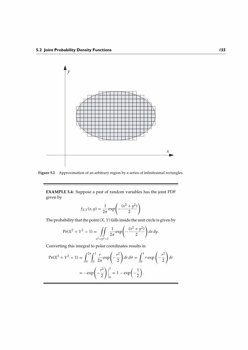
5.2 Joint Probability Density Functions 155
x
y
Figure 5.2 Approximation of an arbitrary region by a series of infinitesimal rectangles.
EXAMPLE 5.4: Suppose a pair of random variables has the joint PDFgiven by
fX,Y(x, y) = 12π
exp
(
− (x2 + y2)2
)
The probability that the point (X, Y) falls inside the unit circle is given by
Pr(X2 + Y2 < 1) =∫∫
x2+y2<1
12π
exp
(
− (x2 + y2)2
)
dx dy.
Converting this integral to polar coordinates results in
Pr(X2 + Y2 < 1) =∫ 2π
0
∫ 1
0
r2π
exp
(
− r2
2
)
dr dθ =∫ 1
0r exp
(
− r2
2
)
dr
= −exp
(
− r2
2
) ∣∣∣∣
1
0= 1 − exp
(
−12
)
.
156 Chapter 5 Pairs of Random Variables
EXAMPLE 5.5: Now suppose that a pair of random variables has thejoint PDF given by
fX,Y(x, y) = c exp(−x − y
2
)u(x)u(y).
First, the constant c is found using the normalization integral∫ ∞
0
∫ ∞
0c exp
(−x − y
2
)dxdy = 1 ⇒ c = 1
2.
Next, suppose we wish to determine the probability of the event{X > Y}. This can be viewed as finding the probability of the pair (X, Y)falling in the region A that is now defined as A = {(x, y) : x > y}. Thisprobability is calculated as
Pr(X > Y) =∫∫
x>y
fX,Y(x, y) dxdy =∫ ∞
0
∫ ∞
y
12
exp(−x − y
2
)dxdy
=∫ ∞
0
12
exp(
−3y2
)
dy = 13
.
EXAMPLE 5.6: In many cases, evaluating the probability of a pairof random variables falling in some region may be quite diffi-cult to calculate analytically. For example, suppose we modifyExample 5.4 so that the joint PDF is now of the form
fX,Y(x, y) = 12π
exp
(
− ((x − 2)2 + (y − 3)2)2
)
.
Again, we would like to evaluate the probability that the pair (X, Y) falls inthe unit circle. To do this analytically we must evaluate
∫∫
x2+y2<1
12π
exp
(
− ((x − 2)2 + (y − 3)2)2
)
dxdy.
Converting to polar coordinates, the integral becomes
∫ 1
0
∫ 2π
0
r2π
exp
(
− ((r cos(θ ) − 2)2 + (r sin(θ ) − 3)2)2
)
dθdr.
5.3 Joint Probability Mass Functions 157
Either way, the double integral looks formidable. We can enlist MATLAB tohelp in one of two ways. First, we could randomly generate many samplesof the pair of random variables according to the specified distribution andcount the relative frequency of the number that fall within the unit circle.Alternatively, we could get MATLAB to calculate one of the preceding doubleintegrals numerically. We will take the latter approach here and evaluatethe double integral in polar coordinates. First, we must define a MATLABfunction to evaluate the integrand:
function out=dblintegrand(q,r)
out=r.*exp(-((r*cos(q)-2).∧2+(r*sin(q)-3).∧2)/2);
MATLAB will then evaluate the integral by executing the command
dblquad(‘dblintegrand’,0,2*pi,0,1)/(2*pi).
By executing these MATLAB commands, we find the value of the integral tobe 0.002072.
5.3 Joint Probability Mass Functions
When the random variables are discrete rather than continuous, it is often moreconvenient to work with probability mass functions rather than PDFs or CDFs. Itis straightforward to extend the concept of the probability mass function to a pairof random variables.
DEFINITION 5.3: The joint probability mass function for a pair of discrete randomvariables X and Y is given by PX,Y(x, y) = Pr({X = x} ∩ {Y = y}).
In particular, suppose the random variable X takes on values from theset {x1, x2, . . . , xM} and the random variable Y takes on values from the set{y1, y2, . . . , yN}. Here, either M and/or N could be potentially infinite, or both couldbe finite. Several properties of the joint probability mass function analogous to thosedeveloped for joint PDFs should be apparent.
(1) 0 ≤ PX,Y(xm, yn) ≤ 1; (5.11a)
(2)M∑
m=1
N∑
n=1
PX,Y(xm, yn) = 1; (5.11b)

158 Chapter 5 Pairs of Random Variables
(3)N∑
n=1
PX,Y(xm, yn) = PX(xm),M∑
m=1
PX,Y(xm, yn) = PY(yn); (5.11c)
(4) Pr((X, Y) ∈ A) =∑
(x,y)
∑
∈ A
PX,Y(x, y). (5.11d)
Furthermore, the joint PDF or the joint CDF of a pair of discrete random vari-ables can be related to the joint PMF through the use of delta functions or stepfunctions by
fX,Y(x, y) =M∑
m=1
N∑
n=1
PX,Y(xm, yn)δ(x − xm)δ(y − ym), (5.12)
FX,Y(x, y) =M∑
m=1
N∑
n=1
PX,Y(xm, yn)u(x − xm)u(y − ym). (5.13)
Usually, it is most convenient to work with PMFs when the random variables arediscrete. However, if the random variables are mixed (i.e., one is discrete and oneis continuous), then it becomes necessary to work with PDFs or CDFs since thePMF will not be meaningful for the continuous random variable.
EXAMPLE 5.7: A pair of discrete random variables N and M have ajoint PMF given by
PN,M(n,m)= (n+m)!n!m!
anbm
(a + b + 1)n+m+1 , m=0,1,2,3, . . . , n=0,1,2,3, . . . .
The marginal PMF of N can be found by summing over m in thejoint PMF:
PN(n) =∞∑
m=0
PN,M(n, m) =∞∑
m=0
(n + m)!n!m!
anbm
(a + b + 1)n+m+1 .
To evaluate this series, the following identity is used:
∞∑
m=0
(n + m)!n!m! xm =
(1
1 − x
)n+1
.

5.4 Conditional Distribution, Density, and Mass Functions 159
The marginal PMF then reduces to
PN(n) = an
(a + b + 1)n+1
∞∑
m=0
(n + m)!n!m!
bm
(a + b + 1)m
= an
(a + b + 1)n+1
1
1 − ba + b + 1
n+1
= an
(1 + a)n+1 .
Likewise, by symmetry, the marginal PMF of M is
PM(m) = bm
(1 + b)m+1 .
Hence, the random variables M and N both follow a geometricdistribution.
5.4 Conditional Distribution, Density,and Mass Functions
The notion of conditional distribution functions and conditional density functionswas first introduced in Chapter 3. In this section, those ideas are extended to the casewhere the conditioning event is related to another random variable. For example,we might want to know the distribution of a random variable representing thescore a student achieves on a test given the value of another random variablerepresenting the number of hours the student studied for the test. Or, perhaps wewant to know the probability density function of the outside temperature giventhat the humidity is known to be below 50 percent.
To start with, consider a pair of discrete random variables X and Y with a PMF,PX,Y(x, y). Suppose we would like to know the PMF of the random variable Xgiven that the value of Y has been observed. Then, according to the definition ofconditional probability:
Pr(X = x|Y = y) = Pr(X = x, Y = y)Pr(Y = y)
= PX,Y(x, y)PY(y)
. (5.14)
We refer to this as the conditional PMF of X given Y. By way of notation we writePX|Y(x|y) = PX,Y(x, y)/PY(y).

160 Chapter 5 Pairs of Random Variables
EXAMPLE 5.8: Using the joint PMF given in Example 5.7, along withthe marginal PMF found in that example, it is found that
PN|M(n|m) = PM,N(m, n)PM(m)
= (n + m)!n!m!
anbm
(a + b + 1)n+m+1(1 + b)m+1
bm
= (n + m)!n!m!
an(1 + b)m+1
(a + b + 1)n+m+1 .
Note that the conditional PMF of N given M is quite different thanthe marginal PMF of N. That is, knowing M changes the distribu-tion of N.
The simple result developed in Equation 5.14 can be extended to the case ofcontinuous random variables and PDFs. The following theorem shows that thePMFs in Equation 5.14 can simply be replaced by PDFs.
THEOREM 5.2: The conditional PDF of a random variable X given that Y = y is
fX|Y(x|y) = fX,Y(x, y)fY(y)
. (5.15)
PROOF: Consider the conditioning event A = y ≤ Y < y + dy. Then
fX|A(x) dx = Pr(x ≤ X < x + dx|y ≤ Y < y + dy)
= Pr(x ≤ X < x + dx, y ≤ Y < y + dy)Pr(y ≤ Y < y + dy)
= fX,Y(x, y) dxdyfY(y) dy
= fX,Y(x, y) dxfY(y)
.
Passing to the limit as dy → 0, the event A becomes the event {Y = y}, producingthe desired result. �
Integrating both sides of this equation with respect to x produces the appropriateresult for CDFs:
FX|Y(x|y) =∫ x−∞ fX,Y(x′, y) dx′
fY(y). (5.16)
Usually, the conditional PDF is much easier to work with, so the conditional CDFwill not be discussed further.

5.4 Conditional Distribution, Density, and Mass Functions 161
EXAMPLE 5.9: A certain pair of random variables has a joint PDFgiven by
fX,Y(x, y) = 2abc(ax + by + c)3 u(x)u(y)
for some positive constants a, b, and c. The marginal PDFs are easilyfound to be
fX(x) =∫ ∞
0fX,Y(x, y) dy = ac
(ax + c)2 u(x)
and
fY(y) =∫ ∞
0fX,Y(x, y) dx = bc
(by + c)2 u(y).
The conditional PDF of X given Y then works out to be
fX|Y(x|y) = fX,Y(x, y)fY(y)
= 2a(by + c)2
(ax + by + c)3 u(x).
The conditional PDF of Y given X could also be determined in asimilar way:
fY|X(y|x) = fX,Y(x, y)fX(x)
= 2b(ax + c)2
(ax + by + c)3 u(y).
EXAMPLE 5.10: This example involves two Gaussian random vari-ables. Suppose X and Y have a joint PDF given by
fX,Y(x, y) = 1
π√
3exp
(
−23
(x2 − xy + y2))
.
The marginal PDF is found as follows:
fX(x) =∫ ∞
−∞fX,Y(x, y) dy = 1
π√
3exp
(
−23
x2)∫ ∞
−∞exp
(
−23
(y2 − xy))
dy.
In order to evaluate the integral, complete the square in the exponent:
fX(x) = 1
π√
3exp
(
−23
x2)
exp
(x2
6
)∫ ∞
−∞exp
(
−23
(
y2 − xy + x2
4
))
dy
= 1
π√
3exp
(
−x2
2
)∫ ∞
−∞exp
(
−23
(y − x
2
)2)
dy.

162 Chapter 5 Pairs of Random Variables
Now the integrand is a Gaussian-looking function. If the appropriateconstant is added to the integrand, the integrand will be a valid PDFand, hence, must integrate out to one. In this case, the constant we needto add to the integrand to make the integral unity is
√2/(3π ). Stated
another way, the integral as just written must evaluate to√
3π/2. Hence,the marginal PDF of X is
fX(x) = 1√2π
exp
(
−x2
2
)
,
and we see that X is a zero-mean, unit-variance, Gaussian (i.e., standardnormal) random variable. By symmetry, the marginal PDF of Y mustalso be of the same form. The conditional PDF of X given Y is
fX|Y(x|y)= fX,Y(x,y)fY(y)
=1
π√
3exp
(
−23
(x2−xy+y2))
1√2π
exp
(
−y2
2
)
=√
23π
exp
(
−23
(
x2−xy+ y2
4
))
=√
23π
exp(
−23
(x− y
2
)2)
.
So, the conditional PDF of X given Y is also Gaussian. But, given that itis known that Y = y, the mean of X is now y/2 (instead of zero), andthe variance of X is 3/4 (instead of one). In this example, knowledge ofY has shifted the mean and reduced the variance of X.
In addition to conditioning on a random variable taking on a point value suchas Y = y, the conditioning can also occur on an interval of the form y1 ≤ Y ≤ y2. Tosimplify notation, let the conditioning event A be A = {y1 ≤ Y ≤ y2}. The relevantconditional PMF, PDF, and CDF are then given respectively by:
PX|A(x) =∑y2
y=y1 PX,Y(x, y)∑y2
y=y1 PY(y); (5.17)
fX|A(x) =∫ y2
y1fX,Y(x, y) dy
∫ y2y1
fY(y) dy; (5.18)
FX|A(x) = FX,Y(x, y2) − FX,Y(x, y1)FY(y2) − FY(y1)
. (5.19)
It is left as an exercise for the reader to derive these expressions.

5.5 Expected Values Involving Pairs of Random Variables 163
EXAMPLE 5.11: Using the joint PDF of Example 5.10, suppose we wantto determine the conditional PDF of X given that Y > yo. The numeratorin Equation 5.18 is calculated according to∫ ∞
yo
fX|Y(x|y) dy =∫ ∞
yo
1
π√
3exp
(
−23
(x2 − xy + y2))
dy
= 1√2π
exp
(
−x2
2
)∫ ∞
yo
√2
3πexp
(
−23
(y − x
2
)2)
dy
= 1√2π
exp
(
−x2
2
)
Q(
2yo − x√3
)
Since the marginal PDF of Y is a zero-mean, unit-variance GaussianPDF, the denominator of Equation 5.18 becomes
∫ ∞
yo
fY(y) dy =∫ ∞
yo
1√2π
exp
(
−y2
2
)
dy = Q(yo).
Therefore, the PDF of X conditioned on Y > yo is
fX|Y>yo (x) = 1√2π
exp
(
−x2
2
) Q(
2yo − x√3
)
Q(yo).
Note that when the conditioning event was a point condition on Y, theconditional PDF of X was Gaussian; yet, when the conditioning eventis an interval condition on Y, the resulting conditional PDF of X is notGaussian at all.
5.5 Expected Values Involving Pairsof Random Variables
The notion of expected value is easily generalized to pairs of random variables.To begin, we define the expected value of an arbitrary function of two randomvariables.

164 Chapter 5 Pairs of Random Variables
DEFINITION 5.4: Let g(x, y) be an arbitrary two-dimensional function. Theexpected value of g(X, Y), where X and Y are random variables, is
E[g(X, Y)] =∞∫∫
−∞g(x, y)fX,Y(x, y) dxdy. (5.20)
For discrete random variables, the equivalent expression in terms of the joint PMF is
E[g(X, Y)] =∑
m
∑
n
g(xm, yn)PX,Y(xm, yn). (5.21)
If the function g(x, y) is actually a function of only a single variable, say x, thenthis definition reduces to the definition of expected values for functions of a singlerandom variable as given in Definition 4.2.
E[g(X)]=∞∫∫
−∞g(x)fX,Y(x,y)dxdy =
∫ ∞
−∞g(x)
[∫ ∞
−∞fX,Y(x,y)dy
]
dx=∫ ∞
−∞g(x)fX(x)dx.
(5.22)
To start with, consider an arbitrary linear function of the two variables g(x, y) =ax + by, where a and b are constants. Then
E[aX + bY] =∞∫∫
−∞[ax + by]fX,Y(x, y) dxdy
= a
∞∫∫
−∞xfX,Y(x, y) dxdy + b
∞∫∫
−∞yfX,Y(x, y) dxdy
= aE[X] + bE[Y]. (5.23)
This result merely states that expectation is a linear operation.In addition to the functions considered in Chapter 4 that led to such statistics
as means, variances, and the like, functions involving both variables x and y willbe considered here. These new functions will lead to statistics that will partiallycharacterize the relationships between the two random variables.
DEFINITION 5.5: The correlation between two random variables is defined as
RX,Y = E[XY] =∞∫∫
−∞xyfX,Y(x, y) dxdy. (5.24)
Furthermore, two random variables that have a correlation of zero are said to beorthogonal.

5.5 Expected Values Involving Pairs of Random Variables 165
One instance in which the correlation appears is in calculating the secondmoment of a sum of two random variables. That is, consider finding the expectedvalue of g(X, Y) = (X + Y)2:
E[(X + Y)2] = E[X2 + 2XY + Y2] = E[X2] + E[Y2] + 2E[XY]. (5.25)
Hence, the second moment of the sum is the sum of the second moment plus twicethe correlation.
DEFINITION 5.6: The covariance between two random variables is
Cov(X, Y) = E[(X − µX)(Y − µY)] =∞∫∫
−∞(x − µX)(y − µY)fX,Y(x, y) dxdy. (5.26)
If two random variables have a covariance of zero, they are said to be uncorrelated.
The correlation and covariance are strongly related to one another as shown by thefollowing theorem.
THEOREM 5.3: Cov(X, Y) = RX,Y − µXµY . (5.27)
PROOF: Cov(X, Y) = E[(X − µX)(Y − µy)] = E[XY − µXY − µYX + µXµY]= E[XY] − µXE[Y] − µYE[X] + µXµY = E[XY] − µXµY .
�As a result, if either X or Y (or both) has a mean of zero, correlation and covarianceare equivalent. The covariance function occurs when calculating the variance ofa sum of two random variables:
Var(X + Y) = Var(X) + Var(Y) + 2Cov(X, Y). (5.28)
This result can be obtained from Equation 5.25 by replacing X with X − µX and Ywith Y − µY .
Another statistical parameter related to a pair of random variables is thecorrelation coefficient, which is nothing more than a normalized version of thecovariance.
DEFINITION 5.7: The correlation coefficient of two random variables X and Y, ρXY ,is defined as
ρXY = Cov(X, Y)√
Var(X)Var(Y)= E[(X − µX)(Y − µY)]
σXσY. (5.29)
The next theorem quantifies the nature of the normalization. In particular, it showsthat a correlation coefficient can never be more than 1 in absolute value.

166 Chapter 5 Pairs of Random Variables
THEOREM 5.4: The correlation coefficient is less than 1 in magnitude.
PROOF: Consider taking the second moment of X+aY, where a is a real constant:
E[(X + aY)2] = E[X2] + 2aE[XY] + a2E[Y2] ≥ 0.
Since this is true for any a, we can tighten the bound by choosing the value of a thatminimizes the left-hand side. This value of a turns out to be
a = −E[XY]E[Y2] .
Plugging in this value gives
E[X2] + (E[XY])2
E[Y2] − 2(E[XY])2
E[Y2] ≥ 0
⇒ (E[XY])2 ≤ E[X2]E[Y2].If we replace X with X − µX and Y with Y − µY , the result is
(Cov(X, Y))2 ≤ Var(X)Var(Y).
Rearranging terms then gives the desired result:
|ρXY | =∣∣∣∣∣
Cov(X, Y)√
Var(X)Var(Y)
∣∣∣∣∣≤ 1. (5.30)
�Note that we can also infer from the proof that equality holds if Y is a constanttimes X. That is, a correlation coefficient of 1 (or −1) implies that X and Y are com-pletely correlated (knowing Y determines X). Furthermore, uncorrelated randomvariables will have a correlation coefficient of zero. Hence, as its name implies,the correlation coefficient is a quantitative measure of the correlation between tworandom variables. It should be emphasized at this point that zero correlation is notto be confused with independence. These two concepts are not the same (more onthis later).
The significance of the correlation, covariance, and correlation coefficient willbe discussed further in the next two sections. For now, we present an exampleshowing how to compute these parameters.
EXAMPLE 5.12: Consider once again the joint PDF of Example 5.10.The correlation for these random variables is
E[XY] =∫ ∞
−∞
∫ ∞
−∞xy
π√
3exp
(
−23
(x2 − xy + y2))
dydx.

5.5 Expected Values Involving Pairs of Random Variables 167
In order to evaluate this integral, the joint PDF is rewritten as fX,Y(x, y) =fY|X(y|x)fX(x) and those terms involving only x are pulled outside theinner integral over y:
E[XY] =∫ ∞
−∞x√2π
exp
(
−x2
2
)[∫ ∞
−∞y
√2
3πexp
(
−23
(y − x
2
)2)
dy
]
dx.
The inner integral (in square brackets) is the expected value of aGaussian random variable with a mean of x/2 and a variance of 3/4which thus evaluates to x/2. Hence,
E[XY] = 12
∫ ∞
−∞x2
√2π
exp
(
−x2
2
)
dx.
The remaining integral is the second moment of a Gaussian randomvariable with zero-mean and unit variance, which thus integrates to 1.The correlation of these two random variables is therefore E[XY] = 1/2.Since both X and Y have zero means, Cov(X, Y) is also equal to 1/2.Finally, the correlation coefficient is also ρXY = 1/2 due to the fact thatboth X and Y have unit variance.
The concepts of correlation and covariance can be generalized to higher ordermoments as given in the following definition.
DEFINITION 5.8: The (m, n)th joint moment of two random variables X and Y is
E[XmYn] =∞∫∫
−∞xmynfX,Y(x, y) dxdy. (5.31)
The (m, n)th joint central moment is similarly defined as
E[(X − µX)m(Y − µY)n] =∞∫∫
−∞(x − µX)m(y − µY)nfX,Y(x, y) dxdy (5.32)
These higher order joint moments are not frequently used and therefore are notconsidered further here.
As with single random variables, a conditional expected value can also bedefined for which the expectation is carried out with respect to the appropriateconditional density function.
DEFINITION 5.9: The conditional expected value of a function g(X) of a randomvariable X given that Y = y is
E[g(X)|Y] =∫ ∞
−∞g(x)fX|Y(x|y) dx. (5.33)

168 Chapter 5 Pairs of Random Variables
Conditional expected values can be particularly useful in calculating expectedvalues of functions of two random variables that can be factored into the prod-uct of two one-dimensional functions. That is, consider a function of the formg(x, y) = g1(x)g2(y). Then
E[g1(X)g2(Y)] =∞∫∫
−∞g1(x)g2(y)fX,Y(x, y) dxdy. (5.34)
From Equation 5.15, the joint PDF is rewritten as fX,Y(x, y) = fY|X(y|x)fX(x),resulting in
E[g1(X)g2(Y)] =∫ ∞
−∞g1(x)fX(x)
[∫ ∞
−∞g2(y)fY|X(y|x) dy
]
dx
=∫ ∞
−∞g1(x)fX(x)EY[g2(Y)|X] dx = EX[g1(X)EY[g2(Y)|X]]. (5.35)
Here the subscripts on the expectation operator have been included for clarity toemphasize that the outer expectation is with respect to the random variable X,while the inner expectation is with respect to the random variable Y (conditionedon X). This result allows us to break a two-dimensional expectation into two one-dimensional expectations. This technique was used in Example 5.12, where thecorrelation between two variables was essentially written as
RX,Y = EX[XEY[Y|X]]. (5.36)
In that example, the conditional PDF of Y given X was Gaussian, and hence findingthe conditional mean was trivial. The outer expectation then required finding thesecond moment of a Gaussian random variable, which is also straightforward.
5.6 Independent Random Variables
The concept of independent events was introduced in Chapter 2. In this section,we extend this concept to the realm of random variables. To make that extension,consider the events A = {X ≤ x} and B = {Y ≤ y} related to the random variables Xand Y. The two events A and B are statistically independent if Pr(A, B) = Pr(A)Pr(B).Restated in terms of the random variables, this condition becomes
Pr(X ≤ x, Y ≤ y) = Pr(X ≤ x)Pr(Y ≤ y) ⇒ FX,Y(x, y) = FX(x)FY(y). (5.37)
Hence, two random variables are statistically independent if their joint CDF factorsinto a product of the marginal CDFs. Differentiating both sides of this equation with

5.6 Independent Random Variables 169
respect to both x and y reveals that the same statement applies to the PDF as well.That is, for statistically independent random variables, the joint PDF factors intoa product of the marginal PDFs:
fX,Y(x, y) = fX(x)fY(y). (5.38)
It is not difficult to show that the same statement applies to PMFs as well. Thepreceding condition can also be restated in terms of conditional PDFs. Dividingboth sides of Equation 5.38 by fX(x) results in
fY|X(y|x) = fY(y). (5.39)
A similar result involving the conditional PDF of X given Y could have beenobtained by dividing both sides by the PDF of Y. In other words, if X and Y areindependent, knowing the value of the random variable X should not change thedistribution of Y and vice versa.
EXAMPLE 5.13: Returning once again to the joint PDF of Example 5.10,we saw in that example that the marginal PDF of X is
fX(x) = 1√2π
exp
(
−x2
2
)
,
while the conditional PDF of X given Y is
fX|Y(x|y) =√
23π
exp(
−23
(x − y
2
)2)
.
Clearly, these two random variables are not independent.
EXAMPLE 5.14: Suppose the random variables X and Y are uniformlydistributed on the square defined by 0 ≤ x, y ≤ 1. That is
fX,Y(x, y) ={
1 0 ≤ x, y ≤ 1
0 otherwise.
The marginal PDFs of X and Y work out to be
fX(x) ={
1 0 ≤ x ≤ 1
0 otherwise, fY(y) =
{1 0 ≤ y ≤ 1
0 otherwise.
These random variables are statistically independent since fX,Y(x, y) =fX(x)fY(y).

170 Chapter 5 Pairs of Random Variables
THEOREM 5.5: Let X and Y be two independent random variables and considerforming two new random variables U = g1(X) and V = g2(Y). These new randomvariables U and V are also independent.
PROOF: To show that U and V are independent, consider the events A = {U ≤ u}and B = {V ≤ v}. Next, define the region Ru to be the set of all points x such thatg1(x) ≤ u. Similarly, define Rv to be the set of all points y such that g2(y) ≤ v. Then
Pr(U ≤ u, V ≤ v) = Pr(X ∈ Ru, Y ∈ Rv) =∫
Rv
∫
Ru
fX,Y(x, y) dxdy.
Since X and Y are independent, their joint PDF can be factored into a product ofmarginal PDFs resulting in
Pr(U ≤ u, V ≤ v) =∫
Ru
fX(x) dx∫
Rv
fY(y) dy
= Pr(X ∈ Ru) Pr(Y ∈ Rv) = Pr(U ≤ u)Pr(V ≤ v).
Since we have shown that FU,V (u, v) = FU(u)FV (v), the random variables U and Vmust be independent. �
Another important result deals with the correlation, covariance, and correlationcoefficients of independent random variables.
THEOREM 5.6: If X and Y are independent random variables, then E[XY] =µXµY , Cov(X, Y) = 0, and ρX,Y = 0.
PROOF:E[XY] =
∞∫∫
−∞xyfX,Y(x, y) dxdy =
∫ ∞
−∞xfX(x) dx
∫ ∞
−∞yfY(y) dy = µXµY .
The conditions involving covariance and correlation coefficient follow directlyfrom this result. �
Therefore, independent random variables are necessarily uncorrelated, but theconverse is not always true. Uncorrelated random variables do not have to beindependent as demonstrated by the next example.
EXAMPLE 5.15: Consider a pair of random variables X and Y that areuniformly distributed over the unit circle so that
fX,Y(x, y) =
1π
x2 + y2 ≤ 1
0 otherwise.
5.6 Independent Random Variables 171
The marginal PDF of X can be found as follows:
fX(x) =∫ ∞
−∞fX,Y(x, y) dy =
∫√
1−x2
−√
1−x2
1π
dy = 2π
√1 − x2, −1 ≤ x ≤ 1.
By symmetry, the marginal PDF of Y must take on the same functionalform. Hence, the product of the marginal PDFs is
fX(x)fY(y) = 4π2
√
(1 − x2)(1 − y2), −1 ≤ x, y ≤ 1.
Clearly, this is not equal to the joint PDF, and hence the two randomvariables are dependent. This conclusion could have been determined ina simpler manner. Note that if we are told that X = 1, then necessarilyY = 0, whereas if we know that X = 0, then Y can range anywherefrom −1 to 1. Therefore, conditioning on different values of X leads todifferent distributions for Y.
Next, the correlation between X and Y is calculated.
E[XY] =∫∫
x2+y2≤1
xyπ
dx dy = 1π
∫ 1
−1x
∫√
1−x2
−√
1−x2y dy
dx
Since the inner integrand is an odd function (of y) and the limits of inte-gration are symmetric about zero, the integral is zero. Hence, E[XY] = 0.Note from the marginal PDFs just found that both X and Y are zero-mean. So, it is seen for this example that while the two random variablesare uncorrelated, they are not independent.
EXAMPLE 5.16: Suppose we wish to use MATLAB to generatesamples of a pair of random variables (X, Y) that are uniformlydistributed over the unit circle. That is, the joint PDF is
fX,Y(x, y) =
1π
x2 + y2 < 1
0 otherwise.
If we generated two random variables independently according to theMATLAB code X=rand(1); Y=rand(1); this would produce a pair ofrandom variables uniformly distributed over the square 0 < x < 1, 0 < y < 1.One way to achieve the desired result is to generate random variablesuniformly over some region that includes the unit circle, and then keep only

172 Chapter 5 Pairs of Random Variables
those pairs of samples which fall inside the unit circle. In this case, it is straight-forward to generate random variables that are uniformly distributed over thesquare −1 < x < 1, −1 < y < 1, which circumscribes the unit circle. Then wekeep only those samples drawn from within this square that also fall withinthe unit circle. The code that follows illustrates this technique. We also showhow to generate a three-dimensional plot of an estimate of the joint PDF fromthe random data generated. To get a decent estimate of the joint PDF, weneed to generate a rather large number of samples (we found that 100,000worked pretty well). This requires that we create and perform several oper-ations on some very large vectors. Doing so tends to make the program runvery slowly. In order to speed up the operation of the program, we choose tocreate shorter vectors of random variables (1,000 in this case) and then repeatthe procedure several times (100 in this case). Although this makes the codea little longer and probably a little harder to follow, by avoiding the creationof very long vectors, it substantially speeds up the program. The results ofthis program are shown in Figure 5.3.
−1.5−1
−0.50
0.51
1.5
−2
−1
0
1
20
0.1
0.2
0.3
0.4
xy
Join
t PD
F
Figure 5.3 Estimate of the joint PDF of a pair of random variables uniformly distributedover the unit circle from the data generated in Example 5.16.

5.6 Independent Random Variables 173
clear
N=1000; % Number of samples per
iteration.
bw=0.1; % Bin widths for histogram.
xbins=[-1.4:bw:1.4];
ybins=[-1.4:bw:1.4]; % Histogram bins.
iterations=100; % Number of iterations.
M=length(xbins);
Nsamples=zeros(M); % Initialize matrix for
storing data.
count=0; % Initialize counter.
for ii=1:iterations
x=2*rand(1,N)-1; y=2*rand(1,N)-1; % Generate variables over
square.
% Keep only those within the unit circle.
X=[]; Y=[];
for k=1:N
if x(k)∧2+y(k)∧2<1X=[X x(k)];
Y=[Y y(k)];
end % End if statement.
end % End k loop.
count=count+length(X); % Count random samples
generated.
% Compute number of samples that fall within each bin.
for m=1:length(xbins)
for n=1:length(ybins)
temp1=(abs(X-xbins(m))<bw/2);
temp2=(abs(Y-ybins(n))<bw/2);
Nsamples(m,n)=Nsamples(m,n)+sum(temp1.*temp2);
end % End n loop.
end % End m loop.
end % End iterations.
PDFest=Nsamples/(count*bw∧2); % Convert to probability
densities.
mesh(xbins,ybins,PDFest) % Plot estimate of joint
PDF.
xlabel(‘x’); ylabel(‘y’); % Label plot axes.
zlabel(‘Joint PDF’);

174 Chapter 5 Pairs of Random Variables
5.7 Jointly Gaussian Random Variables
As with single random variables, the most common and important example of atwo-dimensional probability distribution is that of a joint Gaussian distribution.We begin by defining what is meant by a joint Gaussian distribution.
DEFINITION 5.10: A pair of random variables X and Y are said to be jointlyGaussian if their joint PDF is of the general form
fX,Y(x,y)= 1
2πσXσY
√
1−ρ2XY
×exp
−
(x−µX
σX
)2
−2ρXY
(x−µX
σX
)(y−µY
σY
)
+(
y−µY
σY
)2
2(1−ρ2XY)
(5.40)
where µX and µY are the means of X and Y, respectively; σX and σY are the standarddeviations of X and Y, respectively; and ρXY is the correlation coefficient of X and Y.
It is left as an exercise for the reader to verify that this joint PDF results in marginalPDFs that are Gaussian. That is
fX(x) =∫ ∞
−∞fX,Y(x, y) dy = 1
√
2πσ 2X
exp
(
− (x − µX)2
2σ 2X
)
,
fY(y) =∫ ∞
−∞fX,Y(x, y) dx = 1
√
2πσ 2Y
exp
(
− (y − µY)2
2σ 2Y
)
.
(5.41)
It is also left as an exercise for the reader (see Exercise 5.15) to demonstrate that ifX and Y are jointly Gaussian, then the conditional PDF of X given Y = y is alsoGaussian, with a mean of µX + ρXY(σX/σY)(y − µY) and a variance of σ 2
X(1 − ρ2XY).
An example of this was shown in Example 5.10 and the general case can be provenfollowing the same steps shown in that example.
Figure 5.4 shows the joint Gaussian PDF for three different values of the corre-lation coefficient. In Figure 5.4(a), the correlation coefficient is ρXY = 0, and hencethe two random variables are uncorrelated (and as we will see shortly, indepen-dent). Figure 5.4(b) shows the joint PDF when the correlation coefficient is largeand positive, ρXY = 0. 9. Note how the surface has become taller and thinner and

5.7 Jointly Gaussian Random Variables 175
5
−5
0
−5
0
50
0.02
0.04
0.06
0.08
0.1
0.12
0.14
0.16
xy
f X,Y
(x,
y)
(a)
−5
0
5
−5
0
50
0.05
0.1
0.15
0.2
0.25
0.3
0.35
0.4
f X,Y
(x, y
)
xy
(b)
−5
0
5
−5
0
50
0.05
0.1
0.15
0.2
0.25
0.3
0.35
0.4
f X,Y
(x, y
)
xy
(c)
Figure 5.4 (a) The joint Gaussian PDF: µX = µY = 0, σX = σY = 1, ρXY = 0; (b) thejoint Gaussian PDF: µX = µY = 0, σX = σY = 1, ρXY = 0. 9; (c) the joint Gaussian PDF:µX = µY = 0, σX = σY = 1, ρXY = −0. 9.

176 Chapter 5 Pairs of Random Variables
largely lies above the line y = x. In Figure 5.4(c), the correlation is now largeand negative, ρXY = −0. 9. Note that this is the same image as in Figure 5.4(b),except that it has been rotated by 90◦. Now the surface lies largely above the liney = −x. In all three figures, the means of both X and Y are zero and the variancesof both X and Y are 1. Changing the means would simply translate the surfacebut would not change the shape. Changing the variances would expand or con-tract the surface along either the X or Y axis, depending on which variance waschanged.
EXAMPLE 5.17: The joint Gaussian PDF is given by
fX,Y(x, y) = 1
2πσXσY
√
1 − ρ2XY
exp
(
− 1
2(1 − ρ2XY)
[(x − µX
σX
)2
−2ρXY
(x − µX
σX
)(y − µY
σY
)
+(
y − µY
σY
)2])
.
Suppose we equate the portion of this equation that is within the squarebrackets to a constant. That is
(x − µX
σX
)2
− 2ρXY
(x − µX
σX
)(y − µY
σY
)
+(
y − µY
σY
)2
= c2.
This is the equation for an ellipse. Plotting these ellipses for different valuesof c results in what is known as a contour plot. Figure 5.5 shows such plotsfor the two-dimensional joint Gaussian PDF. The following code can be usedto generate such plots. The reader is encouraged to try creating similar plotsfor different values of the parameters in the Gaussian distribution.
clear
[X,Y]=meshgrid(-8:0.1:8); % Generate x and y array to
% be used for contour plot.
mux=0; muy=0; % Set means.
stdx=3; stdy=3; % Set standard deviations.
varx=stdx∧2; vary=stdy∧2; % Compute variances.
rho=0.5; % Set correlation coefficient.
% Compute exponent of two-dimensional Gaussian PDF.
X1=(X-mux)/stdx;
Y1=(Y-muy)/stdy;
Z=X1.∧2-2*rho*X1.*Y1+Y1.∧2;

5.7 Jointly Gaussian Random Variables 177
−8 −6 −4 −2 0 2 4 6 8−8
−6
−4
−2
0
2
4
6
8
x
y
Figure 5.5 Contour plots for Example 5.17.
c=[1/16 1/4 1 2 4]; % Set contour levels.
contour(X,Y,Z,c) % Produce contour plot grid.
% Turn on grid lines.
xlabel(‘x’); ylabel(‘y’) % Label axes.
THEOREM 5.7: Uncorrelated Gaussian random variables are independent.
PROOF: Uncorrelated Gaussian random variables have a correlation coefficientof zero. Plugging ρXY = 0 into the general joint Gaussian PDF results in
fX,Y(x, y) = 12πσXσY
exp
−
(x − µX
σX
)2
+(
y − µY
σY
)2
2
.
This clearly factors into the product of the marginal Gaussian PDFs.
fX,Y(x, y) = 1√
2πσ 2x
exp
(
− (x − mx)2
2σ 2x
)1
√2πσ 2
y
exp
(
− (y − my)2
2σ 2y
)
= fX(x)fY(y)
�

178 Chapter 5 Pairs of Random Variables
0 1−1
ρXY
Statisticalindependence
LineardependenceY = aX + b,a positive
LineardependenceY = aX + b,a negative
Figure 5.6 Interpretation of the correlation coefficient for jointly Gaussian randomvariables.
While Example 5.15 demonstrates that this property does not hold for all randomvariables, it is true for Gaussian random variables. This allows us to give a strongerinterpretation to the correlation coefficient when dealing with Gaussian randomvariables. Previously it was stated that the correlation coefficient is a quantitativemeasure of the amount of correlation between two variables. While this is true, it isa rather vague statement. After all, what does “correlation” mean? In general, wecannot equate correlation and statistical dependence. Now, however, we see thatin the case of Gaussian random variables, we can make the connection betweencorrelation and statistical dependence. Hence, for jointly Gaussian random vari-ables, the correlation coefficient can indeed be viewed as a quantitative measureof statistical dependence. This relationship is illustrated in Figure 5.6.
5.8 Joint Characteristic and RelatedFunctions
When computing the joint moments of random variables, it is often convenient touse characteristic functions, moment generating functions, or probability generat-ing functions. Since a pair of random variables is involved, the “frequency domain”function must now be two-dimensional. We start with a description of the jointcharacteristic function, which is similar to a two-dimensional Fourier transform ofthe joint PDF.
DEFINITION 5.11: Given a pair of random variables X and Y with a joint PDF,fXY(x, y), the joint characteristic function is
�X,Y(ω1, ω2) = E[e j(ω1X+ω2Y)] =
∞∫∫
−∞e j(ω1x+ω2y)fX,Y(x, y) dxdy. (5.42)

5.8 Joint Characteristic and Related Functions 179
The various joint moments can be evaluated from the joint characteristic functionusing techniques similar to those used for single random variables. It is left as anexercise for the reader to establish the following relationship:
E[XmYn] = (−j)m+n ∂m
∂ωm1
∂n
∂ωn2�X,Y(ω1, ω2)
∣∣∣∣ω1=ω2=0
. (5.43)
EXAMPLE 5.18: Consider a pair of zero-mean, unit-variance, jointlyGaussian random variables whose joint PDF is
fX,Y(x, y) = 1
2π√
1 − ρ2exp
(
− (x2 − 2ρxy + y2)2(1 − ρ2)
)
.
One way to calculate the joint characteristic function is to break theproblem into two one-dimensional problems:
�X,Y(ω1, ω2) = E[e j(ω1X+ω2Y)] = EY
[e jω2YEX
[e jω1X∣∣Y
]].
Conditioned on Y, X is a Gaussian random variable with a mean of ρY
and a variance of 1 − ρ2. The general form of the characteristic function(one-dimensional) of a Gaussian random variable with mean µX andvariance σ 2
X (see Example 4.20) is
�X(ω) = exp
(
jµXω − ω2σ 2X
2
)
.
Hence, the inner expectation evaluates to
EX
[e jω1X∣∣Y
]= exp
(
jρYω1 − ω21(1 − ρ2)
2
)
.
The joint characteristic function is then
�X,Y(ω1, ω2) = EY
[
exp
(
jω2Y + jρYω1 − ω21(1 − ρ2)
2
)]
= exp
(
−ω21(1 − ρ2)
2
)
EY
[e j(ρω1+ω2)Y
].
The remaining expectation is the characteristic function of a zero-mean,unit-variance Gaussian random variable evaluated at ω = ρω1 + ω2.
180 Chapter 5 Pairs of Random Variables
The resulting joint characteristic function is then found to be
�X,Y(ω1, ω2) = exp
(
−ω21(1 − ρ2)
2
)
exp
(
− (ρω1 + ω2)2
2
)
= exp
(
−ω21 + 2ρω1ω2 + ω2
22
)
.
From this expression, various joint moments can be found. For example,the correlation is
E[XY] = − ∂
∂ω1
∂
∂ω2exp
(
−ω21 + 2ρω1ω2 + ω2
22
) ∣∣∣∣ω1=ω2=0
= ∂
∂ω2ρω2exp
(
−ω22
2
) ∣∣∣∣ω2=0
= ρ.
Since the two random variables were zero-mean, Cov(X, Y) = ρ.Furthermore, since the two random variables were unit variance, ρ
is also the correlation coefficient. We have therefore proved that theparameter ρ that shows up in the joint Gaussian PDF is indeed thecorrelation coefficient.
We could easily compute higher order moments as well. For exam-ple, suppose we need to compute E[X2Y2]. It can be computed in asimilar manner to the preceding:
E[X2Y2] = ∂2
∂ω21
∂2
∂ω22
exp
(
−ω21 + 2ρω1ω2 + ω2
22
) ∣∣∣∣ω1=ω2=0
= − ∂2
∂ω22
[1 − (ρω2)2]exp
(
−ω22
2
) ∣∣∣∣ω2=0
= 1 + 2ρ2.
DEFINITION 5.12: For a pair of discrete random variables defined on a two-dimensional lattice of nonnegative integers, one can define a joint probabilitygenerating function as
HX,Y(z1, z2) = E[zX
1 zY2
]=
∞∑
m=0
∞∑
n=0
PX,Y(m, n)zm1 zn
2 . (5.44)
The reader should be able to show that the joint partial derivatives of the jointprobability generating function evaluated at zero are related to the terms in thejoint probability mass function, whereas those same derivatives evaluated at 1 lead

5.8 Joint Characteristic and Related Functions 181
to joint factorial moments. Specifically,
PX,Y(k, l) = 1k!l!
∂k
∂zk1
∂ l
∂zl2
HX,Y(z1, z2)∣∣∣∣z1=z2=0
, (5.45)
E[X(X − 1) · · · (X − k + 1)Y(Y − 1) · · · (Y − l + 1)] = ∂k
∂zk1
∂ l
∂zl2
HX,Y(z1, z2)∣∣∣∣z1=z2=1
.
(5.46)
EXAMPLE 5.19: Consider the joint PMF given in Example 5.7:
PN,M(n, m) = (n + m)!n!m!
anbm
(a + b + 1)n+m+1 .
It is not too difficult to work out the joint probability generating func-tion for this pair of discrete random variables.
HN,M(z1z2)=∞∑
n=0
∞∑
m=0
(n+m)!n!m!
(az1)n(bz2)m
(a+b+1)n+m+1
=∞∑
n=0
(az1)n
(a+b+1)n+1
∞∑
m=0
(n+m)!n!m!
(bz2
a+b+1
)m
=∞∑
n=0
(az1)n
(a+b+1)n+1
1
1− bz2
a+b+1
n+1
=∞∑
n=0
(az1)n
(a+b(1−z2)+1)n+1
= 1a+b(1−z2)+1
∞∑
n=0
(az1
a+b(1−z2)+1
)n
= 11+a(1−z1)+b(1−z2)
It should be noted that the closed form expression used for the variouspreceding series limits the range in the (z1, z2) plane for which theseexpressions are valid; thus, care must be taken when evaluating thisfunction and its derivatives at various points. However, for this exam-ple, the expression is valid in and around the points of interest (i.e.,(z1, z2) = (0, 0) and (z1, z2) = (1, 1)).
Now that the joint probability generating function has been found,joint moments are fairly easy to compute. For example,
E[NM] = ∂
∂z1
∂
∂z2
11 + a(1 − z1) + b(1 − z2)
∣∣∣∣z1=z2=1
= ∂
∂z1
b[1 + a(1 − z1)]2
∣∣∣∣z1=1
= 2ab,

182 Chapter 5 Pairs of Random Variables
E[N(N − 1)M] = ∂2
∂z21
∂
∂z2
11 + a(1 − z1) + b(1 − z2)
∣∣∣∣z1=z2=1
= ∂2
∂z21
b[1 + a(1 − z1)]2
∣∣∣∣z1=1
= 6a2b.
Putting these two results together, it is found that
E[N2M] = E[N(N − 1)M] + E[NM] = 6a2b + 2ab.
By symmetry, we can also conclude that E[NM(M − 1)] = 6ab2 andE[NM2] = 6ab2 + 2ab. As one last example, we note that
E[N(N − 1)M(M − 1)] = ∂2
∂z21
∂2
∂z22
11 + a(1 − z1) + b(1 − z2)
∣∣∣∣z1=z2=1
= ∂2
∂z21
2b2
[1 + a(1 − z1)]3
∣∣∣∣z1=1
= 24a2b2.
From this and the previous results, we can find E[N2M2] as follows:
E[N2M2] = E[N(N − 1)M(M − 1)] + E[NM2] + E[N2M] − E[NM]= 24a2b2 + 6ab2 + 6a2b + 2ab.
The moment generating function can also be generalized in a manner virtuallyidentical to what was done for the characteristic function. We leave the details ofthis extension to the reader.
5.9 Transformations of Pairs of RandomVariables
In this section, we consider forming a new random variable as a function of a pairof random variables. When a pair of random variables is involved, there are twoclasses of such transformations. The first class of problems deals with the case wherea single new variable is created as a function of two random variables. The secondclass of problems involves creating two new random variables as two functions oftwo random variables. These two distinct but related problems are treated in thissection.

5.9 Transformations of Pairs of Random Variables 183
Consider first a single function of two random variables, Z = g(X, Y). If the jointPDF of X and Y is known, can the PDF of the new random variable Z be found? Ofcourse, the answer is yes, and there are a variety of techniques to solve these typesof problems depending on the nature of the function g(·). The first technique to bedeveloped is an extension of the approach we used in Chapter 4 for functions ofa single random variable.
The CDF of Z can be expressed in terms of the variables X and Y as
FZ(z) = Pr(Z ≤ z) = Pr(g(X, Y) ≤ z) =∫∫
g(x,y)≤z
fX,Y(x, y) dxdy. (5.47)
The inequality g(x, y) ≤ z defines a region in the (x, y) plane. By integrating thejoint PDF of X and Y over that region, the CDF of Z is found. The PDF can then befound by differentiating with respect to z. In principle, one can use this techniquewith any transformation; however, the integral to be computed may or may not beanalytically tractable, depending on the specific joint PDF and the transformation.
To illustrate, consider a simple yet very important example where the transfor-mation is just the sum of the random variables, Z = X + Y. Then
FZ(z) =∫∫
x+y≤z
fX,Y(x, y) dxdy =∫ ∞
−∞
∫ z−y
−∞fX,Y(x, y) dxdy. (5.48)
Differentiating to form the PDF results in
fZ(z) = ddz
∫ ∞
−∞
∫ z−y
−∞fX,Y(x, y) dxdy =
∫ ∞
−∞fX,Y(z − y, y) dy. (5.49)
The last step in Equation 5.49 is completed using Liebnitz’s rule1. An importantspecial case results when X and Y are independent. In this case, the joint PDFfactors into the product of the marginals, producing
fZ(z) =∫ ∞
−∞fX(z − y)fY(y) dy. (5.50)
Note that this integral is a convolution. Thus, the following important result hasbeen proved:
THEOREM 5.8: If X and Y are statistically independent random variables, thenthe PDF of Z = X + Y is given by the convolution of the PDFs of X and Y, fZ(z) =fX(z) ∗ fY(z).
1Liebnitz’s rule states that
∂
∂x
∫ b(x)
a(x)f (x, y) dy = ∂b
∂xf (x, b(x)) − ∂a
∂xf (x, a(x)) +
∫ b(x)
a(x)
∂
∂xf (x, y) dy.

184 Chapter 5 Pairs of Random Variables
EXAMPLE 5.20: Suppose X and Y are independent and both haveexponential distributions,
fX(x) = a exp(−ax)u(x), fY(y) = b exp(−by)u(y).
The PDF of Z = X + Y is then found by performing the necessaryconvolution:
fZ(z)=∫ ∞
−∞fX(z−y)fY(y)dy =ab
∫ ∞
−∞exp(−a(z−y))exp(−by)u(z−y)u(y)dy
=abe−az∫ z
0exp((a−b)y)dyu(z)
= aba−b
[
e−aze(a−b)y∣∣∣∣
y=z
y=0
]
u(z)= aba−b
[e−by −e−az
]u(z).
This result is valid assuming that a �= b. If a = b, then the convolutionworks out to be
fZ(z) = a2ze−azu(z).
Students familiar with the study of signals and systems should recall that theconvolution integral appears in the context of passing signals through linear time-invariant systems. In that context, most students develop a healthy respect for theconvolution and will realize that quite often the convolution can be a cumbersomeoperation. To avoid difficult convolutions, these problems can often be solved usinga frequency domain approach in which a Fourier or Laplace transform is invokedto replace the convolution with a much simpler multiplication. In the context ofprobability, the characteristic function or the moment generating function can fulfillthe same role. Instead of finding the PDF of Z = X + Y directly via convolution,suppose we first find the characteristic function of Z:
�Z(ω) = E[e jωZ] = E
[e jω(X+Y)] = E
[e jωXe jωY]. (5.51)
If X and Y are independent, then the expected value of the product of a function ofX times a function of Y factors into the product of expected values:
�Z(ω) = E[e jωX]E
[e jωY] = �X(ω)�Y(ω). (5.52)
Once the characteristic function of Z is found, the PDF can be found using aninverse Fourier transform.

5.9 Transformations of Pairs of Random Variables 185
Again, the characteristic function can be used to simplify the amount of com-putation involved in calculating PDFs of sums of independent random variables.Furthermore, we have also developed a new approach to find the PDFs of a gen-eral function of two random variables. Returning to a general transformation ofthe form Z = g(X, Y), one can first find the characteristic function of Z according to
�Z(ω) = E[e jωg(X,Y)] =
∞∫∫
−∞e jωg(x,y)fX,Y(x, y) dxdy. (5.53)
An inverse transform of this characteristic function will then produce the desiredPDF. In some cases, this method will provide a simpler approach to the problem,while in other cases the direct method may be easier.
EXAMPLE 5.21: Suppose X and Y are independent, zero-mean, unitvariance Gaussian random variables. The PDF of Z = X2 + Y2
can be found using either of the methods described thus far. Usingcharacteristic functions,
�Z(ω) = E[e jω(X2+Y2)] = E
[e jωX2]
E[e jωY2]
.
The expected values are evaluated as follows:
E[e jωX2] =
∫ ∞
−∞1√2π
e jωx2e−x2/2 dx
= 1√
1 − 2jω
∫ ∞
−∞
√1 − 2jω
2πe−(1−2jω)x2/2 dx = 1
√1 − 2jω
.
The last step is accomplished using the normalization integral forGaussian functions. The other expected value is identical to the firstsince X and Y have identical distributions. Hence,
�Z(ω) =(
1√
1 − 2jω
)2
= 11 − 2jω
.
The PDF is found from the inverse Fourier transform to be
fZ(z) = 12
exp(−x
2
)u(x).
The other approach is to find the CDF as follows:
FZ(z) = Pr(X2 + Y2 ≤ z) =∫∫
x2+y2≤z
12π
exp
(
−x2 + y2
2
)
dxdy.

186 Chapter 5 Pairs of Random Variables
Converting to polar coordinates,
FZ(z) =∫ √
z
0
∫ 2π
0
r2π
exp
(
− r2
2
)
dθdru(z)
=∫ √
z
0r exp
(
− r2
2
)
dru(z) =[1 − exp
(− z
2
)]u(z).
Finally, differentiating with respect to z results in
fZ(z) = ddz
[1 − exp
(− z
2
)]u(z) = 1
2exp
(− z
2
)u(z).
Another approach to solving these types of problems uses conditional distribu-tions. Consider a general transformation, Z = g(X, Y). Next, suppose we conditionon one of the two variables, say X = x. Conditioned on X = x, Z = g(x, Y) isnow a single variable transformation. Hence, the conditional PDF of Z given X canbe found using the general techniques presented in Chapter 4. Once fZ|X(z|x) isknown, the desired (unconditional) PDF of Z can be found according to
fZ(z) =∫ ∞
−∞fZ,X(z, x) dx =
∫ ∞
−∞fZ|X(z|x)fX(x) dx. (5.54)
EXAMPLE 5.22: Suppose X and Y are independent zero-mean, unit-variance Gaussian random variables and we want to find the PDF ofZ = Y/X. Conditioned on X = x, the transformation Z = Y/x is asimple linear transformation and
fZ|X(z|x) = |x|fY(xz) = |x|√2π
exp
(
−x2z2
2
)
.
Multiplying the conditional PDF by the marginal PDF of X andintegrating out x gives the desired marginal PDF of Z.
fZ(z)=∫ ∞
−∞fZ|X(z|x)fX(x)dx=
∫ ∞
−∞|x|√2π
exp
(
−x2z2
2
)1√2π
exp
(
−x2
2
)
dx
= 12π
∫ ∞
−∞|x|exp
(
−(1+x2)z2
2
)
dx
= 1π
∫ ∞
0xexp
(
−(1+z2)x2
2
)
dx= 1π
11+z2

5.9 Transformations of Pairs of Random Variables 187
Evaluating the integral in the last step can be accomplished by mak-ing the substitution u = (1 + z2)x2/2. Hence, the quotient of twoindependent Gaussian random variables follows a Cauchy distribution.
Up to this point, three methods have been developed for finding the PDF ofZ = g(X, Y) given the joint PDF of X and Y; they can be summarized as follows.
5.9.1 Method 1, CDF Approach
Define a set R(z) = {(x, y): g(x, y) ≤ z}. The CDF of Z is the integral of the jointPDF of X and Y over the region R(z). The PDF is then found by differentiating theexpression for the CDF:
fZ(z) = ddz
∫∫
R(z)
fX,Y(x, y) dx dy. (5.55)
5.9.2 Method 2, Characteristic Function Approach
First, find the characteristic function of Z according to
�Z(ω) = E[e jωg(X,Y)]. (5.56)
Then compute the inverse transform to get the PDF of Z.
5.9.3 Method 3, Conditional PDF Approach
Fix either X = x or Y = y (whichever is more convenient). The conditional PDF ofZ can then be found using the techniques developed for single random variablesin Chapter 4. Once the conditional PDF of Z is found, the unconditional PDF isgiven by
fZ(z) =∫ ∞
−∞fZ|Y(z|y)fY(y) dy or fZ(z) =
∫ ∞
−∞fZ|X(z|x)fX(x) dx. (5.57)
Next, our attention moves to solving a slightly more general class of problems.Given two random variables X and Y, suppose we now create two new randomvariables W and Z according to some 2 × 2 transformation of the general form
Z = g1(X, Y),
W = g2(X, Y). (5.58)

188 Chapter 5 Pairs of Random Variables
The most common example of this type of problem involves changing coordinatesystems. Suppose, for example, that the variables X and Y represent the randomposition of some object in Cartesian coordinates. In some problems, it may beeasier to view the object in a polar coordinate system, in which case two newvariables R and could be created to describe the location of the object in polarcoordinates. Given the joint PDF of X and Y, how can we find the joint PDF ofR and ?
The procedure for finding the joint PDF of Z and W for a general transformationof the form given in Equation 5.58 is an extension of the technique used for a 1 × 1transformation. First, recall the definition of the joint PDF given in Equation 5.2,which states that for an infinitesimal region Ax,y = (x, x + εx) × (y, y + εy), the jointPDF, fX,Y(x, y), has the interpretation
Pr((X, Y) ∈ Ax,y) = fX,Y(x, y)εxεy = fX,Y(x, y)(Area of Ax,y). (5.59)
Assume for now that the transformation is invertible. In that case, the transfor-mation maps the region Ax,y into a corresponding region Az,w in the (z, w)-plane.Furthermore,
Pr((X, Y) ∈ Ax,y) = Pr((Z, W ) ∈ Az,w) = fZ,W (z, w)(Area of Az,w). (5.60)
Putting the two previous equations together results in
fZ,W (z, w) = fX,Y(x, y)Area of Ax,y
Area of Az,w. (5.61)
A fundamental result of multivariable calculus states that if a transformation ofthe form given in Equation 5.58 maps an infinitesimal region Ax,y, to a region Az,w,then the ratio of the areas of these regions is given by the absolute value of theJacobian of the transformation:
Area of Ax,y
Area of Az,w=∣∣∣∣J(
x yz w
)∣∣∣∣ =
∣∣∣∣∣∣∣∣
det
∂x∂z
∂y∂z
∂x∂w
∂y∂w
∣∣∣∣∣∣∣∣
. (5.62)
The PDF of Z and W is then given by
fZ,W (z, w) = fX,Y(x, y)∣∣∣∣J(
x yz w
)∣∣∣∣ . (5.63)

5.9 Transformations of Pairs of Random Variables 189
If it is more convenient to take derivatives of z and w with respect to x and y ratherthan vice versa, we can alternatively use
Area of Az,w
Area of Ax,y=∣∣∣∣J(
z wx y
)∣∣∣∣ =
∣∣∣∣∣∣∣∣∣
det
∂z∂x
∂z∂y
∂w∂x
∂w∂y
∣∣∣∣∣∣∣∣∣
, (5.64)
fZ,W (z, w) = fX,Y(x, y)∣∣∣∣J(
z wx y
)∣∣∣∣
. (5.65)
Whether Equation 5.63 or 5.65 is used, any expressions involving x or y mustbe replaced with the corresponding functions of z and w. Let the inversetransformation of Equation 5.58 be written as
X = h1(Z, W ),
Y = h2(Z, W ).(5.66)
Then these results can be summarized as
fZ,W (z, w) = fX,Y(x, y)∣∣∣∣J(
z wx y
)∣∣∣∣ x = h1(z, w)
y = h2(z, w)
= fX,Y(x, y)∣∣∣∣J(
x yz w
)∣∣∣∣
x = h1(z, w)y = h2(z, w)
(5.67)
If the original transformation is not invertible, then the inverse transformation mayhave multiple roots. In this case, as with transformations involving single randomvariables, the expression in Equation 5.67 must be evaluated at each root of theinverse transformation and the results summed together. This general procedurefor transforming pairs of random variables is demonstrated next through a fewexamples.
EXAMPLE 5.23: A classical example of this type of problem involvesthe transformation of two independent Gaussian random variablesfrom Cartesian to polar coordinates. Suppose
fX,Y(x, y) = 12πσ 2 exp
(
−x2 + y2
2σ 2
)
.
We seek the PDF of the polar magnitude and phase given by
R =√
X2 + Y2,
= tan−1(Y/X).

190 Chapter 5 Pairs of Random Variables
The inverse transformation is
X = R cos(),
Y = R sin().
In this case, the inverse transformation takes on a simpler functionalform and so we elect to use this form to compute the Jacobian.
J(
x yr θ
)
= det
∂x∂r
∂x∂θ
∂y∂r
∂y∂θ
= det
[cos(θ ) −r sin(θ )
sin(θ ) r cos(θ )
]
= r cos2(θ ) + r sin2(θ ) = r
The joint PDF of R and is then
fR,(r, θ ) = fX,Y(x, y)∣∣∣∣J(
x yr θ
)∣∣∣∣
x = h1(r, θ )y = h2(r, θ )
= r2πσ 2 exp
(
−x2 + y2
2σ 2
)
x = r cos(θ )y = r sin(θ )
= r2πσ 2 exp
(
− r2
2σ 2
)
,r ≥ 0
0 ≤ θ < 2π.
Note that in these calculations, we do not have to worry about takingthe absolute value of the Jacobian since for this problem the Jacobian(= r) is always nonnegative. If we were interested, we could also findthe marginal distributions of R and to be
fR(r) = rσ 2 exp
(
− r2
2σ 2
)
u(r) and f(θ ) = 12π
, 0 ≤ θ < 2π .
The magnitude follows a Rayleigh distribution while the phase isuniformly distributed over (0, 2π ).
EXAMPLE 5.24: Suppose X and Y are independent and both uniformlydistributed over (0, 1), so that
fX,Y(x, y) ={
1 0 ≤ x, y < 1
0 otherwise.

5.9 Transformations of Pairs of Random Variables 191
Consider forming the two new random variables
Z =√
−2 ln(X) cos(2πY),
W =√
−2 ln(X) sin(2πY).
The inverse transformation in this case is found to be
X = exp
(Z2 + W 2
2
)
,
Y = 12π
tan−1(
WZ
)
.
In this example, we will compute the Jacobian by taking derivatives ofz and w with respect to x and y to produce
J(
z wx y
)
= det
∂z∂x
∂z∂y
∂w∂x
∂w∂y
= det
−1x
cos(2πy)√−2 ln(x)
−2π√−2 ln(X) sin(2πY)
−1x
sin(2πy)√−2 ln(x)
2π√−2 ln(X) cos(2πY)
= −2π
x
[cos2(2πy) + sin2(2πy)
]= −2π
x.
Note that since x is always nonnegative, the absolute value of theJacobian will just be 2π/x. The joint PDF of Z and W is then foundto be
fZ,W (z, w) = fX,Y(x, y)∣∣∣∣J(
z wx y
)∣∣∣∣ x = h1(z, w)
y = h2(z, w)
= x2π x = exp
(
− z2+w22
)
y = 12π
tan−1(wz)
= 12π
exp
(
−z2 + w2
2
)
.
This transformation is known as the Box-Muller transformation. It trans-forms a pair of independent uniform random variables into a pair ofindependent Gaussian random variables. This transformation has appli-cation in the world of computer simulations. Techniques for generating

192 Chapter 5 Pairs of Random Variables
uniform random variables are well known. This transformation thenallows us to generate Gaussian random variables as well. More materialon this subject is given in Chapter 12, Simulation Techniques.
EXAMPLE 5.25: Suppose X and Y are independent Gaussian randomvariables, both with zero mean and unit variance. Two new randomvariables, Z and W, are formed through a linear transformation ofthe form
Z = aX + bY,
W = cX + dY.
The inverse transformation is given by
X = dad − bc
Z − bad − bc
W ,
Y = − cad − bc
Z + aad − bc
W .
With this general linear transformation, the various partial derivativesare trivial to compute and the resulting Jacobian is
J(
z wx y
)
= det[
a bc d
]
= ad − bc.
Plugging these results into the general formula results in
fZ,W (z, w) = fX,Y(x, y)∣∣∣∣J(
z wx y
)∣∣∣∣ x = h1(z, w)
y = h2(z, w)
=1
2πexp
(− x2+y2
2
)
|ad − bc|x = d
ad−bc z − bad−bc w
y = cad−bc z + a
ad−bc w.
= 1
2π√
(ad − bc)2exp
(
− (c2 + d2)z2 − 2(bd + ac)zw + ((a2 + b2)w)2
2(ad − bc)2
)
With a little algebraic manipulation, it can be shown that this joint PDFfits the general form of a joint Gaussian PDF. In particular,
fZ,W (z, w) = 1
2πσZσW
√
1 − ρ2ZW
× exp
(
− (z/σZ)2 − 2ρZW (z/σZ)(w/σw) + (w/σw)2
2(1 − ρ2ZW )
)
,

5.10 Complex Random Variables 193
where σ 2Z = a2 + b2, σ 2
W = c2 + d2, and ρ2ZW = (ac + bd)2(a2 + b2)−1
(c2 + d2)−1.
A few remarks about the significance of the result of Example 5.25 are appropriate.First, we have performed an arbitrary linear transformation on a pair of indepen-dent Gaussian random variables and produced a new pair of Gaussian randomvariables (which are no longer independent). In the next chapter, it will be shownthat a linear transformation of any number of jointly Gaussian random variablesalways produces jointly Gaussian random variables. Second, if we look at thisproblem in reverse, two correlated Gaussian random variables Z and W can betransformed into a pair of uncorrelated Gaussian random variables X and Y usingan appropriate linear transformation. More information will be given on this topicin the next chapter as well.
5.10 Complex Random Variables
In engineering practice, it is common to work with quantities that are complex.Usually, a complex quantity is just a convenient shorthand notation for work-ing with two real quantities. For example, a sinusoidal signal with amplitude, A,frequency, ω, and phase, θ , can be written as
s(t) = A cos(ωt + θ ) = Re[Ae jθ e jωt
], (5.68)
where j = √−1. The complex number Z = Ae jθ is known as a phasor rep-resentation of the sinusoidal signal. It is a complex number with real part ofX = Re[Z] = A cos(θ ) and imaginary part of Y = Im[Z] = A sin(θ ). The phasor Zcan be constructed from two real quantities (either A and θ or X and Y).
Suppose a complex quantity that we are studying is composed of two real quan-tities that happen to be random. For example, the preceding sinusoidal signal mighthave a random amplitude and/or a random phase. In either case, the complex num-ber Z will also be random. Unfortunately, our formulation of random variables doesnot allow for complex quantities. When we began to describe a random variable viaits CDF in the beginning of Chapter 3, the CDF was defined as FZ(z) = Pr(Z ≤ z).This definition makes no sense if Z is a complex number: what does it mean for acomplex number to be less than another number? Nevertheless, the engineeringliterature is filled with complex random variables and their distributions.
The concept of a complex random variable can often be the source of greatconfusion to many students, but it doesn’t have to be as long as we realize that

194 Chapter 5 Pairs of Random Variables
a complex random variable is nothing more than a shorthand representation oftwo real random variables. To motivate the concept of a complex random variable,we use the most common example of a pair of independent, equal variance, jointlyGaussian random variables X and Y. The joint PDF is of the form
fX,Y(x, y) = 12πσ 2 exp
(
− (x − µX)2 + (y − µY)2
2σ 2
)
. (5.69)
This joint PDF (of two real random variables) naturally lends itself to be writtenin terms of some complex variables. Define Z = X + jY, z = x + jy, and µZ =µX + jµY . Then
fX,Y(x, y) = fZ(z) = 12πσ 2 exp
(
−|z − µZ|22σ 2
)
. (5.70)
We reemphasize at this point that this is not to be interpreted as the PDF of acomplex random variable (since such an interpretation would make no sense);rather, this is just a compact representation of the joint PDF of two real randomvariables. This density is known as the circular Gaussian density function (since thecontours of fZ(z) = constant form circles in the complex z-plane).
Note that the PDF in Equation 5.70 has two parameters, µZ and σ . The para-meter µZ is interpreted as the mean of the complex quantity, Z = X + jY:
µZ = E[Z] = E[X + jY] =∫ ∞
−∞(x + jy)fX,Y(x, y) dxdy = µX + jµY . (5.71)
But what about σ 2? We would like to be able to interpret it as the variance ofZ = X + jY. To do so, we need to redefine what we mean by variance of a complexquantity. If we used the definition we are used to (for real quantities), we wouldfind
E[(Z − µZ)2] = E{[(X − µX) + j(Y − µY)]2} = Var(X) − Var(Y) + 2j Cov(X, Y).(5.72)
In the case of our independent Gaussian random variables, since Cov(X, Y) = 0and Var(X) = Var(Y), this would lead to E[(Z − µZ)2] = 0. To overcome thisinconsistency, we redefine the variance for a complex quantity as follows.
DEFINITION 5.13: For a complex random quantity, Z = X + jY, the variance isdefined as
Var(Z) = 12
E[|Z − µZ|2
]= 1
2Var(X) + 1
2Var(Y). (5.73)

5.11 Engineering Application: Mutual Information, Channel Capacity, and Channel Coding 195
We emphasize at this point that this definition is somewhat arbitrary and waschosen so that the parameter σ 2 that shows up in Equation 5.70 can be interpreted asthe variance of Z. Many textbooks do not include the factor of 1/2 in the definition,while many others (besides this one) do include the 1/2. Hence, there seems to beno way to avoid a little bit of confusion here. The student just needs to be awarethat there are two inconsistent definitions prevalent in the literature.
DEFINITION 5.14: For two complex random variables Z1 = X1 + jY1 and Z2 =X2 + jY2, the correlation and covariance are defined as
R1,2 = 12
E[Z1Z∗2] = 1
2{E[X1X2] + E[Y1Y2] − jE[X1Y2] + jE[X2Y1]}, (5.74)
C1,2 = 12
E[(Z1 − µZ1 )(Z2 − µZ2 )∗]. (5.75)
As with real random variables, complex quantities are said to be orthogonal if theircorrelation is zero, whereas they are uncorrelated if their covariance is zero.
5.11 Engineering Application: MutualInformation, Channel Capacity,and Channel Coding
In Section 4.12, we introduced the idea of the entropy of a random variable thatis a quantitative measure of how much randomness there is in a specific randomvariable. If the random variable represents the output of a source, the entropytells us how much mathematical information there is in each source symbol. Wecan also construct similar quantities to describe the relationships between randomvariables. Consider two random variables X and Y that are statistically dependentupon one another. Each random variable has a certain entropy associated with it,H(X) and H(Y), respectively. Suppose it is observed that Y = y. Since X and Yare related, knowing Y will tell us something about X, and hence the amount ofrandomness in X will be changed. This could be quantified using the concept ofconditional entropy.
DEFINITION 5.15: The conditional entropy of a discrete random variable X givenknowledge of a particular realization of a related random variable Y = y is
H(X|Y = y) =∑
x
Pr(X = x|Y = y) log(
1Pr(X = x|Y = y)
)
. (5.76)
196 Chapter 5 Pairs of Random Variables
Averaging over all possible conditioning events produces
H(X|Y) =∑
x
∑
y
Pr(Y = y)Pr(X = x|Y = y) log(
1Pr(X = x|Y = y)
)
=∑
x
∑
y
Pr(X = x, Y = y) log(
1Pr(X = x|Y = y)
)
. (5.77)
The conditional entropy tells how much uncertainty remains in the random variableX after we observe the random variable Y. The amount of information providedabout X by observing Y can be determined by forming the difference between theentropy in X before and after observing Y.
DEFINITION 5.16: The mutual information between two discrete random variablesX and Y is
I(X; Y) = H(X) − H(X|Y) =∑
x
∑
y
Pr(X = x, Y = y) log(
Pr(X = x|Y = y)Pr(X = x)
)
.
(5.78)
We leave it as an exercise for the reader to prove the following properties of mutualinformation:
• Nonnegative: I(X; Y) ≥ 0.• Independence: I(X; Y) = 0 if and only if X and Y are independent.• Symmetry: I(X; Y) = I(Y; X).
Now we apply the concept of mutual information to a digital communicationsystem. Suppose we have some digital communication system that takes digitalsymbols from some source (or from the output of a source encoder) and transmitsthem via some modulation format over some communications medium. At thereceiver, a signal is received and processed and ultimately a decision is made asto what symbol(s) was most likely sent. We will not concern ourselves with thedetails of how the system operates, but rather we will model the entire process in aprobabilistic sense. Let X represent the symbol to be sent, which is randomly drawnfrom some n-letter alphabet according to some distribution p = (p0, p1, . . . , pn−1).Furthermore, let Y represent the decision made by the receiver, with Y taken to bea random variable on an m-letter alphabet. It is not unusual to have m �= n, butin order to keep this discussion as simple as possible, we will consider only thecase where m = n so that the input and output of our communication system aretaken from the same alphabet. Also, we assume the system to be memoryless sothat decisions made on one symbol are not affected by previous decisions, nor dothey affect future decisions. In this case, we can describe the operation of the digital

5.11 Engineering Application: Mutual Information, Channel Capacity, and Channel Coding 197
0
1
2
0
1
2
q0, 0
q1,0q2,0
0,2
q0, 1
q1, 1
q2,1
q
q1,2
q2, 2
Q
q0, 0 q0, 1 q0, 2
q1, 0 q1, 1 q1, 2
q2, 0 q2, 1 q2, 2
=
Figure 5.7 A transition diagram for a ternary (three-letter) communication channel.
communication system using a transition diagram as illustrated in Figure 5.7 for athree-letter alphabet. Mathematically, the operation of this communication systemcan be described by a matrix Q whose elements are qi,j = Pr(Y = i|X = j).
We can now ask ourselves how much information the communication systemcan carry. Or, in other words, if we observe the output of the system, how muchinformation does this give us about what was really sent? The mutual informationanswers this question. In terms of the channel (as described by Q) and the input(as described by p), the mutual information is
I(X, Y) =∑
i
∑
j
pjqi,j log
(qi,j
pj
)
. (5.79)
Note that the amount of information carried by the system is a function not only ofthe channel but also of the source. As an extreme example, suppose the input dis-tribution were p = (1, 0, . . . , 0). In that case it is easy to show that I(X, Y) = 0; thatis, the communication system carries no information. This is not because the com-munication system is incapable of carrying information, but because what we arefeeding into the system contains no information. To describe the information car-rying capability of a communication channel, we need a quantity that is a functionof the channel only and not of the input to the channel.
DEFINITION 5.17: Given a discrete communications channel described by atransition probability matrix Q, the channel capacity is given by
C = maxp
I(X; Y) = maxp
∑
i
∑
j
pjqi,j log
(qi,j
pj
)
. (5.80)
The maximization of the mutual information is with respect to any valid probabilitydistribution p.

198 Chapter 5 Pairs of Random Variables
EXAMPLE 5.26: As a simple example, consider the so-called binarysymmetric channel (BSC) described by the transition probability matrix
Q =[
1 − q qq 1 − q
]
.
The BSC is described by a single parameter q, which has the interpreta-tion of the probability of bit error of the binary communications system.That is, q is the probability of the receiver deciding a 0 was sent when a1 was actually sent, and it is also the probability of the receiver decidinga 1 was sent when a 0 was actually sent. Since the input to this channelis binary, its distribution can also be described by a single parameter.That is, p = (p, 1 − p). The mutual information for the BSC is
I(X; Y) = p(1 − q) log(
1 − qp
)
+ pq log(
qp
)
+ (1 − p)(1 − q) log(
1 − q1 − p
)
+ (1 − p)q log(
q1 − p
)
.
Some straightforward algebraic manipulations reveal that this expres-sion can be simplified to I(X; Y) = H(p) − H(q), where H(·) isthe binary entropy function. Maximization with respect to p is nowstraightforward. The mutual information is maximized when the inputdistribution is p = (0. 5, 0. 5) and the resulting capacity is
C = 1 − H(q).
This function is illustrated in Figure 5.8.
The channel capacity provides a fundamental limitation on the amount of infor-mation that can reliably be sent over a channel. For example, suppose we wantedto transmit information across the binary symmetric channel of Example 5.26.Furthermore, suppose the error probability of the channel was q = 0. 1. Then thecapacity is C = 1 − H(0. 1) = 0. 53 bit. That is, every physical bit that is transmittedacross the channel must contain less than 0.53 bit of mathematical information. Thisis achieved through the use of redundancy via channel coding. Consider the blockdiagram of the digital communication system in Figure 5.9. The binary source pro-duces independent but identically distributed (i.i.d., or IID) bits that are equallylikely to be 0 or 1. (We will discuss IID random variables further in Chapter 7.)This source has an entropy of 1 bit/source symbol. Since the channel has a capac-ity of 0.53 bit, the information content of the source must be reduced before these

5.11 Engineering Application: Mutual Information, Channel Capacity, and Channel Coding 199
0 0.2 0.4 0.6 0.8 10
0.1
0.2
0.3
0.4
0.5
0.6
0.7
0.8
0.9
1
q
C=
1–H
(q)
Figure 5.8 Capacity of a binary symmetric channel.
Binarysource
(n, k)encoder
BSCq=0.1
Decoder Destination
Figure 5.9 A functional block diagram of a digital communications system.
symbols are sent across the channel. This is achieved by the channel coder, whichtakes blocks of k information bits and maps them to n-bit code words where n > k.Each code word contains k bits of information and so each coded bit contains k/nbits of mathematical information. By choosing the code rate, k/n, to be less thanthe channel capacity, C, we can assure that the information content of the symbolsbeing input to the channel is no greater than the information-carrying capability ofthe channel.
Viewed from a little more concrete perspective, the channel used to transmitphysical bits has an error rate of 10 percent. The purpose of the channel code is toadd redundancy to the data stream to provide the ability to correct the occasionalerrors caused by the channel. A fundamental result of information theory knownas the channel coding theorem states that as k and n go to infinity in such a waythat k/n < C, it is possible to construct a channel code (along with the appropriatedecoder) that will provide error-free communication. That is, the original informa-tion bits will be provided to the destination with an arbitrarily small probability oferror. The channel coding theorem does not tell us how to construct such a code,but significant progress has been made in recent years toward finding practicaltechniques to achieve what information theory promises is possible.

200 Chapter 5 Pairs of Random Variables
Exercises5.1 For positive constants a and b, a pair of random variables has a joint PDF
specified by
fX,Y(x, y) = abe−(ax+by) u(x) u(y).
(a) Find the joint CDF, FX,Y(x, y).
(b) Find the marginal PDFs, fX(x) and fY(y).
(c) Find Pr(X > Y).
(d) Find Pr(X > Y2).
5.2 For positive constants a, b, c, and positive integer n, a pair of randomvariables has a joint PDF specified by
fX,Y(x, y) = d(ax + by + c)n u(x) u(y).
(a) Find the constant d in terms of a, b, c, and n.
(b) Find the marginal PDFs, fX(x) and fY(y).
(c) Find Pr(X > Y).
5.3 A pair of random variables has a joint PDF specified by
fX,Y(x, y) = d exp(−(ax2 + bxy + cy2)).
(a) Find the constant d in terms of a, b, and c. Also find any restrictionsneeded for a , b, and c themselves for this to be a valid PDF.
(b) Find the marginal PDFs, fX(x) and fY(y).
(c) Find Pr(X > Y).
5.4 A pair of random variables has a joint PDF specified by
fX,Y(x, y) =
c√
1 − x2 − y2 x2 + y2 ≤ 1
0 otherwise.
(a) Find the constant c.
(b) Find Pr(X2 + Y2 > 1/4).
(c) Find Pr(X > Y).

Exercises 201
5.5 A pair of random variables has a joint PDF specified by
fX,Y(x, y) = 18π
exp
(
− (x − 1)2 + (y + 1)2
8
)
.
(a) Find Pr(X > 2, Y < 0).(b) Find Pr(0 < X < 2, |Y + 1| > 2).(c) Find Pr(Y > X). Hint: Set up the appropriate double integral and then
use the change of variables: u = x − y, v = x + y.
5.6 For some integer L and constant c, two discrete random variables have ajoint PMF given by
PM,N(m, n) ={
c m ≥ 0, n ≥ 0, m + n < L
0 otherwise.
(a) Find the value of the constant c in terms of L.(b) Find the marginal PMFs, PM(m) and PN(n).(c) Find Pr(M + N < L/2).
5.7 A pair of random variables has a joint PDF specified by
fX,Y(x, y) = 1
2π√
3exp
(
−x2 + 2xy + 4y2
6
)
.
(a) Find the marginal PDFs, fX(x) and fY(y).(b) Based on the results of part (a), find E[X], E[Y], Var(X), and Var(Y).(c) Find the conditional PDF, fX|Y(x|y).(d) Based on the results of part (c), find E[XY], Cov(X, Y), and ρX,Y .
5.8 A pair of random variables is uniformly distributed over the ellipsedefined by x2 + 4y2 ≤ 1.
(a) Find the marginal PDFs, fX(x) and fY(y).(b) Based on the results of part (a), find E[X], E[Y], Var(X), and Var(Y).(c) Find the conditional PDFs, fX|Y(x|y) and fY|X(y|x).(d) Based on the results of part (c), find E[XY], Cov(X, Y), and ρX,Y .
5.9 Prove that if two random variables are linearly related (i.e., Y = aX + b forconstants a �= 0 and b), then
ρX,Y = sgn(a) ={
1 if a > 0
−1 if a < 0.

202 Chapter 5 Pairs of Random Variables
Also, prove that if two random variables have∣∣ρX,Y
∣∣ = 1, then they are
linearly related.
5.10 Prove the triangle inequality that states that√
E[(X + Y)2] ≤√
E[X2] +√
E[Y2].
5.11 Two random variables X and Y have, µX = 2, µY = −1, σX = 1, σY = 4,and ρX,Y = 1/4. Let U = X + 2Y and V = 2X − Y. Find the followingquantities:
(a) E[U] and E[V];(b) E[U2], E[V2], Var(U), and Var(V);(c) E[UV], Cov(U, V), and ρU,V .
5.12 Suppose two random variables are related by Y = aX2 and assume thatfX(x) is symmetric about the origin. Show that ρX,Y = 0.
5.13 Find an example (other than the one given in Example 5.15) of two randomvariables that are uncorrelated but not independent.
5.14 Starting from the general form of the joint Gaussian PDF given in Equation5.40, show that the resulting marginal PDFs are both Gaussian.
5.15 Starting from the general form of the joint Gaussian PDF given in Equation5.40 and using the results of Exercise 5.14, show that conditioned on Y = y,X is Gaussian with a mean of µX + ρXY(σX/σY)(y − µY) and a variance ofσ 2
X(1 − ρ2XY).
5.16 Let X and Y be random variables with means µX and µY , variances σ 2X and
σ 2Y , and correlation coefficient ρX,Y .
(a) Find the value of the constant a which minimizes [E(Y − aX)2].(b) Find the value of [E(Y − aX)2] when a is given as determined in
part (a).
5.17 Let X and Y be zero-mean random variables with a correlation coefficientof ρ and unequal variances of σ 2
X and σ 2Y .
(a) Find the joint characteristic function, �X,Y(ω1, ω2).(b) Find the correlation, covariance, and correlation coefficient.(c) Find E[X2Y2].

Exercises 203
5.18 Find the general form of the joint characteristic function of two jointlyGaussian random variables.
5.19 A quarterback throws a football at a target marked out on the ground 40yards from his position. Assume that the PDF for the football’s hitting thetarget is Gaussian within the plane of the target. Let the coordinates of theplane of the target be denoted by the x and y axes. Thus, the joint PDF of(X, Y) is a two-dimensional Gaussian PDF. The average location of the hitsis at the origin of the target, and the standard deviation in each directionis the same and is denoted as σ . Assuming X and Y are independent, findthe probability that the hits will be located within an annular ring of widthdr located a distance r from the origin; that is, find the probability densityfunction for hits as a function of the radius from the origin.
5.20 Let X and Y be independent and both exponentially distributed with
fX(v) = fY(v) = be−bv u(v).
Find the PDF of Z = X − Y.
5.21 Let X and Y be jointly Gaussian random variables. Show that Z = aX + bYis also a Gaussian random variable. Hence, any linear transformation oftwo Gaussian random variables produces a Gaussian random variable.
5.22 Let X and Y be jointly Gaussian random variables with E[X] = 1, E[Y] =−2, Var(X) = 4, Var(Y) = 9, and ρX,Y = 1/3. Find the PDF of Z =2X − 3Y − 5. Hint: To simplify this problem, use the result of Exercise 5.21.
5.23 Let X and Y be independent Rayleigh random variables such that
fX(v) = fY(v) = v exp
(
−v2
2
)
u(v).
(a) Find the PDF of Z = max(X, Y).(b) Find the PDF of W = min(X, Y).
5.24 Suppose X and Y are independent and exponentially distributed both withunit-mean. Consider the roots of the quadratic equation z2 + Xz + Y = 0.
(a) Find the probability that the roots are real.(b) Find the probability that the roots are complex.(c) Find the probability that the roots are equal.
204 Chapter 5 Pairs of Random Variables
5.25 Suppose X is a Rayleigh random variable and Y is an arcsine randomvariable, so that
fX(x) = xσ 2 exp
(
− x2
2σ 2
)
u(x) and fY(y) = 1
π
√
1 − y2|y| < 1.
Furthermore, assume X and Y are independent. Find the PDF of Z = XY.
5.26 Let X and Y be independent and both uniformly distributed over (0, 2π ).Find the PDF of Z = (X + Y) mod 2π .
5.27 Let X be a Gaussian random variable, and let Y be a Bernoulli randomvariable with Pr(Y = 1) = p and Pr(Y = −1) = 1 − p. If X and Y areindependent, find the PDF of Z = XY. Under what conditions is Z aGaussian random variable?
5.28 Let X and Y be independent zero-mean, unit-variance Gaussian randomvariables. Consider forming the new random variable U, V according to
U = X cos(θ ) − Y sin(θ ),
V = X sin(θ ) + Y cos(θ ).
Note that this transformation produces a coordinate rotation through anangle of (θ ). Find the joint PDF of U and V. Hint: The result of Example5.25 will be helpful here.
5.29 Let X and Y be zero-mean, unit-variance Gaussian random variables withcorrelation coefficient, ρ. Suppose we form two new random variablesusing a linear transformation:
U = aX + bY,
V = cX + dY.
Find constraints on the constants a, b, c, and d such that U and V areindependent.
5.30 Suppose X and Y are independent and Gaussian with means of µX andµY , respectively, and equal variances of σ 2. The polar variables are formedaccording to R =
√X2 + Y2 and = tan−1(Y/X).
(a) Find the joint PDF of R and .(b) Show that the marginal PDF of R follows a Rician distribution.

MATLAB Exercises 205
5.31 Suppose X and Y are independent, zero-mean Gaussian random variableswith variances of σ 2
X and σ 2Y , respectively. Find the joint PDF of
Z = X2 + Y2 and W = Z2 − Y2.
5.32 Suppose X and Y are independent, Cauchy random variables. Find thejoint PDF of
Z = X2 + Y2 and W = XY.
5.33 A complex random variable is defined by Z = Ae j, where A and areindependent and is uniformly distributed over (0, 2π ).
(a) Find E[Z].(b) Find Var(Z). For this part, leave your answer in terms of the moments
of A.
5.34 Suppose Q =
0. 8 0. 1 0. 10. 1 0. 8 0. 10. 1 0. 1 0. 8
in Figure 5.7 and pi = 1/3, i = 1, 2, 3.
Determine the mutual information for this channel.
5.35 Repeat the previous problem if Q =
0. 9 0. 1 00 0. 9 0. 10 0. 1 0. 9
.
5.36 Repeat Exercise 5.35 if Q =
1/3 1/3 1/31/3 1/3 1/31/3 1/3 1/3
. Can you give an interpre-
tation for your result?
MATLAB Exercises5.37 Provide contour plots for the ellipses discussed in Example 5.17. Consider
the following cases:
(a) σX = σY and ρXY = 0;(b) σX < σY and ρXY = 0;(c) σX > σY and ρXY = 0;(d) σX = σY and ρXY �= 0.

206 Chapter 5 Pairs of Random Variables
Let c2 be the same for each case. Discuss the effect that σX , σY , and ρXY ,have on the shape of the contour. Now select one of the cases and let c2
increase and decrease. What is the significance of c2?
5.38 Let X and Y have a joint PDF given by
fX,Y(x, y) = 12π
exp
(
− ((x − 2)2 + (y − 3)2)2
)
as in Example 5.6. Write a MATLAB program to generate many samples ofthis pair of random variables. Note that X and Y are independent, Gaussianrandom variables with unit variances and means of 2 and 3, respectively.After a large number of sample pairs have been generated, compute therelative frequency of the number of pairs that fall within the unit circle,X2 + Y2 < 1. Compare your answer with that obtained in Example 5.6.How many random samples must you generate in order to get a decentestimate of the probability?
5.39 Let X and Y have a joint PDF given by
fX,Y(x, y) = 12π
exp
(
− ((x − 1)2 + y2)2
)
.
Write a MATLAB program to evaluate Pr((X, Y ∈ �)), where � is theshaded region bounded by the lines y = x and y = −x, as shown in theaccompanying figure. You should set up the appropriate double integraland use MATLAB to evaluate the integral numerically. Note in this casethat one of the limits of integration is infinite. How will you deal with this?
x
y
ℜ
y = −x
y = x
5.40 Write a MATLAB program to generate pairs of random variables that areuniformly distributed over the ellipse x2 + 4y2 < 1. Use the techniqueemployed in Example 5.16. Also, create a three-dimensional plot of anestimate of the PDF obtained from the random data you generated.

Multiple Random Variables 6
In many applications, it is necessary to deal with a large number of random vari-ables. Often, the number of variables can be arbitrary. In this chapter, the conceptsdeveloped previously for single random variables and pairs of random variablesare extended to allow for an arbitrary number of random variables. Much of thefocus of this chapter is on multidimensional Gaussian random variables, since mostnon-Gaussian random variables are difficult to deal with in many dimensions. Oneof our main goals here is to develop a vector/matrix notation that will allow us torepresent potentially large sequences of random variables with a compact notation.Many of the concepts developed in Chapter 5 can be extended to multiple dimen-sions in a very straightforward manner; thus we will devote minimal time to thoseconcepts in our current discussion. Rather, attention is focused on those ideas thatrequire more than a trivial extension to the work done in previous chapters.
6.1 Joint and Conditional PMFs, CDFs,and PDFs
The concepts of probability mass function, conditional distribution function, andprobability density function are easily extended to an arbitrary number of randomvariables. Their definitions follow.
DEFINITION 6.1: For a set of N random variables X1, X2, . . . , XN , the joint PMF,CDF, and PDF are given respectively by
PX1, X2, ..., XN (xk1 , xk2 , . . . , xkN ) = Pr(X1 = xk1 , X2 = xk2 , . . . , XN = xkN ); (6.1)
207

208 Chapter 6 Multiple Random Variables
FX1, X2, ..., XN (x1, x2, . . . , xN) = Pr(X1 ≤ x1, X2 ≤ x2, . . . , XN ≤ xN); (6.2)
fX1, X2, ..., XN (x1, x2, . . . , xN) = ∂N
∂x1∂x2 . . . ∂xNFX1, X2,..., XN (x1, x2, . . . , xN). (6.3)
When large numbers of random variables are involved, this notation can get cum-bersome, so it is convenient to introduce a vector notation to write these quantitiesin a more compact fashion. Let X = [X1, X2, . . . , XN]T be a column vector1consistingof the N random variables and similarly define x = [x1, x2, . . . , xN]T . Then thepreceding functions can be expressed respectively as PX(x), FX(x), and fX(x).
Marginal CDFs can be found for a subset of the variables by evaluating the jointCDF at infinity for the unwanted variables. For example,
FX1, X2, ..., XM (x1, x2, . . . , xM) = FX1, X2, ..., XN (x1, x2, . . . , xM , ∞, ∞, . . . , ∞). (6.4)
Marginal PDFs are found from the joint PDF by integrating out the unwantedvariables. Similarly, marginal PMFs are obtained from the joint PMF by summingout the unwanted variables:
fX1, X2, ...,XM (x1,x2, . . . , xM)=∫ ∞∫
−∞. . .∫
fX1,X2, ...,XN (x1,x2, . . . ,xN)dxM+1dxM+2 . . . dxN ,
(6.5)
PX1, X2, ..., XM (xk1 , xk2 , . . . , xkM ) =∑kM+1
∑kM+2
. . .∑kN
PX1, X2,..., XN (xk1 , xk2 , . . . , xkN ). (6.6)
Similar to that done for pairs of random variables in Chapter 5, we can alsoestablish conditional PMFs and PDFs.
DEFINITION 6.2: For a set of N random variables X1, X2, . . . , XN , the conditionalPMF and PDF of X1, X2, . . . , XM conditioned on XM+1, XM+2, . . . , XN are given by
PX1,..., XM |XM+1,..., XN (xk1 , . . . , xkM | xkM+1 , . . . , xkN ) = Pr(X1 = xk1 , . . . , XN = xkN )Pr(XM+1 = xkM+1 , . . . , XN = xkN )
,
(6.7)
fX1,..., XM |XM+1,..., XN (x1, . . . , xM|xM+1, . . . , xN) = fX1, . . . , XN(x1, . . . , xN)fXM+1 , . . . , XN(xM+1, . . . , xN)
. (6.8)
1We use T to represent the matrix transpose operation so that if v is a row vector, then vT
is a column vector. Also, to avoid confusion throughout the text, we use boldface variablesto represent vector and matrix quantities and regular face variables for scalar quantities.
6.2 Expectations Involving Multiple Random Variables 209
Using conditional PDFs, many interesting factorization results can be establishedfor joint PDFs involving multiple random variables. For example, consider fourrandom variables, X1, X2, X3, X4:
fX1, X2, X3, X4 (x1, x2, x3, x4) = fX1|X2, X3, X4 (x1 | x2, x3, x4)fX2, X3, X4 (x2, x3, x4)
= fX1|X2, X3, X4 (x1 | x2, x3, x4)fX2|X3, X4 (x2 | x3, x4)fX3, X4 (x3, x4)
= fX1|X2, X3,X4 (x1 | x2, x3, x4)fX2|X3, X4 (x2 | x3, x4)fX3|X4 (x3 | x4)fX4 (x4). (6.9)
Almost endless other possibilities exist as well.
DEFINITION 6.3: A set of N random variables is statistically independent if anysubset of the random variables are independent of any other disjoint subset. Inparticular, any joint PDF of M ≤ N variables should factor into a product of thecorresponding marginal PDFs.
As an example, consider three random variables, X, Y, Z. For these three randomvariables to be independent, we must have each pair independent. This impliesthat
fX, Y(x, y) = fX(x)fY(y), fX, Z(x, z) = fX(x)fZ(z), fY, Z(y, z) = fY(y)fZ(z). (6.10)
In addition, the joint PDF of all three must also factor into a product of the marginals,
fX, Y, Z(x, y, z) = fX(x)fY(y)fZ(z). (6.11)
Note that all three conditions in Equation 6.10 follow directly from the single condi-tion in Equation 6.11. Hence, Equation 6.11 is a necessary and sufficient conditionfor three variables to be statistically independent. Naturally, this result can beextended to any number of variables. That is, the elements of a random vectorX = [X1, X2, . . . , XN]T are independent if
fX(x) =N∏
n = 1
fXn (xn). (6.12)
6.2 Expectations Involving MultipleRandom Variables
For a vector of random variables X = [X1, X2, . . . , XN]T , we can construct a cor-responding mean vector that is a column vector of the same dimension and

210 Chapter 6 Multiple Random Variables
whose components are the means of the elements of X. Mathematically, we sayµ = E[X] = [E[X1], E[X2], . . . , E[XN]]T . Two other important quantities associ-ated with the random vector are the correlation and covariance matrices. (To beconsistent, the vector µ should be bold; however, we have elected not to do so.)
DEFINITION 6.4: For a random vector X = [X1, X2, . . . , XN]T , the correlationmatrix is defined as RXX = E[XXT ]. That is, the (i, j)th element of the N × Nmatrix RXX is E[XiXj]. Similarly, the covariance matrix is defined as CXX =E[(X − µ)(X − µ)T ] so that the (i, j)th element of CXX is Cov(Xi, Xj).
THEOREM 6.1: Correlation matrices and covariance matrices are symmetric andpositive definite.
PROOF: Recall that a square matrix, RXX, is symmetric if RXX = RTXX. Equiva-
lently, the (i, j)th element must be the same as the (j, i)th element. This is clearly thecase here since E[XiXj] = E[XjXi]. Recall that the matrix RXX is positive definite ifzTRXXz > 0 for any vector z such that ||z|| > 0.
zTRXXz = zTE[XXT ]z = E[zTXXTz] = E[(zTX)2]. (6.13)
Note that zTX is a scalar random variable (a linear combination of the componentsof X). Since the second moment of any random variable is positive (except forthe pathological case of a random variable that is identically equal to zero), thenthe correlation matrix is positive definite. As an aside, this also implies that theeigenvalues of the correlation matrix are all positive. Identical steps can be followedto prove the same properties hold for the covariance matrix. �
Next, consider a linear transformation of a vector random variable. That is,create a new set of M random variables, Y = [Y1, Y2, . . . , YM]T , according to
Y1 = a1, 1X1 + a1, 2X2 + · · · + a1, NXN + b1,
Y2 = a2, 1X1 + a2, 2X2 + · · · + a2, NXN + b2,
· · ·YM = aM, 1X1 + aM, 2X2 + · · · + aM, NXN + bM .
(6.14)
The number of new variables, M, does not have to be the same as the numberof original variables, N. To write this type of linear transformation in a compactfashion, define a matrix A whose (i, j)th element is the coefficient ai,j and a col-umn vector, b = [b1, b2, . . . , bM]T . Then the linear transformation of Equation 6.14is written in vector/matrix form as Y = AX + b. The next theorem describesthe relationship between the means of X and Y and the correlation matrices ofX and Y.

6.3 Gaussian Random Variables in Multiple Dimensions 211
THEOREM 6.2: For a linear transformation of vector random variables of the formY = AX + b, the means of X and Y are related by
µY = AµX + b. (6.15)
Also, the correlation matrices of X and Y are related by
RYY = ARXXAT + AµXbT + bµTXAT + bbT , (6.16)
and the covariance matrices of X and Y are related by
CYY = ACXXAT . (6.17)
PROOF: For the mean vector,
µY = E[Y] = E[AX + b] = AE[X] + b = AµX + b. (6.18)
Similarly, for the correlation matrix,
RYY = E[YYT ] = E[(AX + b)(AX + b)T ]= E[AXXTAT ] + E[bXTAT ] + E[AXbT ] + E[bbT ]= AE[XXT ]AT + bE[XT ]AT + AE[X]bT + bbT
= ARXXAT + AµXbT + bµTXAT + bbT . (6.19)
To prove the result for the covariance matrix, write Y − µY as
Y − µY = (AX + b) − (AµX + b) = A(X − µX). (6.20)
Then,
CYY = E[(Y − µY)(Y − µY)T ] = E[{A(X − µX)}{A(X − µX)}T ]= E[A(X − µX)(X − µX)TAT ] = AE[(X − µX)(X − µX)T ]AT = ACXXAT .
(6.21)
�
6.3 Gaussian Random Variables inMultiple Dimensions
Recall from the study of two-dimensional random variables in the previous chap-ter that the functional form of the joint Gaussian PDF was fairly complicated.
212 Chapter 6 Multiple Random Variables
It would seem that the prospects of forming a joint Gaussian PDF for an arbitrarynumber of dimensions are grim. However, the vector/matrix notation developedin the previous sections make this task manageable and, in fact, the resulting jointGaussian PDF is quite simple.
DEFINITION 6.5: The joint Gaussian PDF for a vector of N random variables, X,with mean vector µX and covariance matrix CXX is given by2
fX(x) = 1√(2π )Ndet(CXX)
exp(
−12
(x − µX)TC−1XX(x − µX)
). (6.22)
EXAMPLE 6.1: To demonstrate the use of this matrix notation, supposeX is a two-element vector and the mean vector and covariance matrixare given by their general forms
µX =[µ1µ2
]and CXX =
[σ 2
1 ρσ1σ2ρσ1σ2 σ 2
2
].
The determinant of the covariance matrix is
det(CXX) = σ 21 σ 2
2 − (ρσ1σ2)2 = σ 21 σ 2
2 (1 − ρ2),
while the inverse is
C−1XX =
[σ 2
2 −ρσ1σ2−ρσ1σ2 σ 2
1
]
σ 21 σ 2
2 (1 − ρ2)=
[σ−2
1 −ρσ−11 σ−1
2−ρσ−1
1 σ−12 σ−2
2
]
(1 − ρ2).
The quadratic form in the exponent then works out to be
(x − µX)TC−1XX(x − µX)
= [x1 − µ1x2 − µ2
][
σ−21 −ρσ−1
1 σ−12
−ρσ−11 σ−1
2 σ−22
]
(1 − ρ2)
[x1 − µ1x2 − µ2
]
=
(x1 − µ1
σ1
)2
− 2ρ
(x1 − µ1
σ1
)(x2 − µ2
σ2
)+(
x2 − µ2
σ2
)2
(1 − ρ2).
2The notation det(A) refers to the determinant of the matrix A, while A−1 is the inverseof A.

6.3 Gaussian Random Variables in Multiple Dimensions 213
Plugging all these results into the general form for the joint GaussianPDF gives
fX1, X2 (x1, x2) = 1√(2π )2σ 2
1 σ 22 (1 − ρ2)
× exp
−
(x1 − µ1
σ1
)2
− 2ρ
(x1 − µ1
σ1
)(x2 − µ2
σ2
)+(
x2 − µ2
σ2
)2
2(1 − ρ2)
.
This is exactly the form of the two-dimensional joint Gaussian PDF givenin the previous chapter.
EXAMPLE 6.2: As a special case, suppose a vector of N jointly Gaus-sian random variables are all mutually uncorrelated. This means thatCov(Xi, Xj) = 0 for all i �= j. A direct result of this is that all of theoff-diagonal elements of the covariance matrix of X are zero. In otherwords, CXX is a diagonal matrix of the general form
CXX =
σ 21 0 . . . 00 σ 2
2 . . . 0. . . . . . . . .0 0 . . . σ 2
N
.
The determinant of a diagonal matrix is the product of the diagonalentries so that in this case det(CXX) = σ 2
1 σ 22 . . . σ 2
N . The inverse is alsotrivial to compute and takes on the form
C−1XX =
σ−21 0 . . . 00 σ−2
2 . . . 0. . . . . . . . .0 0 . . . σ−2
N
.

214 Chapter 6 Multiple Random Variables
The quadratic form that appears in the exponent of the Gaussian PDFbecomes
(x − µX)TC−1XX(x − µX)
= [x1 − µ1x2 − µ2 . . . xN − µN
]
σ−21 0 . . . 00 σ−2
2 . . . 0. . . . . . . . .0 0 . . . σ−2
N
x1 − µ1x2 − µ2
. . .xN − µN
=N∑
n=1
(xn − µn
σn
)2
.
The joint Gaussian PDF for a vector of uncorrelated random variablesis then
fX(x) = 1√(2π )nσ 2
1 σ 22 . . . σ 2
N
exp
(−1
2
N∑n=1
(xn − µn
σn
)2)
=N∏
n=1
1√2πσ 2
n
exp
(− (xn − µn)2
2σ 2n
).
This shows that for any number of uncorrelated Gaussian random vari-ables, the joint PDF factors into the product of marginal PDFs, andhence uncorrelated Gaussian random variables are independent. Thisis a generalization of the same result that was proved in Chapter 5 fortwo Gaussian random variables.
EXAMPLE 6.3: In this example, we use MATLAB’s symboliccapabilities to compute the form of a three-dimensional GaussianPDF. Suppose we have three jointly Gaussian random variables[X, Y, Z]T with a mean vector µ = [1, 2, 3]T and covariance matrix
C =9 4 1
4 9 41 4 9
.

6.4 Transformations Involving Multiple Random Variables 215
The three-dimensional joint PDF, fX, Y, Z(x, y, z), can be found with thefollowing MATLAB code:
x=sym(’x’,’real’); % Define x, y, and z as symbolic.
y=sym(’y’,’real’);
z=sym(’z’,’real’);
pi=sym(’pi’); % Disable numeric definition of pi.
C=[9 4 1; 4 9 4; 1 4 9]; % Covariance matrix.
mu=[1; 2; 3]; % Mean vector.
% Compute PDF symbolically.
v=[x; y; z]-mu;
f=exp(-v’*(inv(C))*v/2)/sqrt((2*pi)∧3*det(C));simplify(f)
Executing this program, MATLAB finds the joint PDF to be
fX, Y, Z(x, y, z) = 1
464√
58π3exp
(− 65
928x2 + 11
232x − 125
232+ 2
29xy
+ 229
y − 7464
xz + 69232
z − 558
y2 + 229
yz − 65928
z2)
.
The reader is encouraged to try different mean vectors and covariancematrices in the preceding program.
6.4 Transformations Involving MultipleRandom Variables
In this section, we discuss various transformations of vector random variables. Toexhaustively cover this topic would require much more space than we can devoteto it here. Instead, we chose to cover some of the more common transformationsencountered in engineering practice. To start with, we extend the formula for 2 × 2transformations developed in the previous chapter to the case of N ×N transforms.Let Y = g(X) be a vector transformation,
Y1 = g1(X1, X2, . . . , XN),
Y2 = g2(X1, X2, . . . , XN),
. . . (6.23)
YN = gN(X1, X2, . . . , XN),

216 Chapter 6 Multiple Random Variables
and let X = h(Y) be the inverse transformation. Given the PDF of X, the PDF of Yis found by
fY(y) = fX(x)∣∣∣∣det[
J(
y1 y2 . . . yN
x1 x2 . . . xN
)] ∣∣∣∣
∣∣∣∣∣∣∣∣∣x = h(y)
= fX(x)∣∣∣∣det
[J(
x1 x2 . . . xN
y1 y2 . . . yN
)] ∣∣∣∣∣∣∣∣x = h(y)
. (6.24)
As in Chapter 5, it needs to be understood that if the transformation is not one-to-one, the preceding expression must be evaluated at each root and summed together.This result can be proved using the same sort of derivation that was used for thecase of 2 × 2 transformations.
6.4.1 Linear Transformations
Perhaps the single most important class of transformations is that involving lineartransformations of Gaussian random variables. Consider a linear transformationof the general form Y = AX+b when the random vector X has a joint Gaussian PDFas given in Equation 6.22. To begin, consider the case where the dimensionalityof X and Y are the same (i.e., both are N-element vectors). In that case, the matrixA is a square matrix. Furthermore, it is assumed that the matrix A is invertible(det(A) �= 0). In this case, the Jacobian of the linear transformation is
J(
y1 y2 . . . yN
x1 x2 . . . xN
)=
∂y1
∂x1
∂y1
∂x2. . .
∂y1
∂xN
∂y2
∂x1
∂y2
∂x2. . .
∂y2
∂xN. . . . . . . . .∂yN
∂x1
∂yN
∂x2. . .
∂yN
∂xN
=
a1, 1 a1, 2 . . . a1, N
a2, 1 a2, 2 . . . a2, N
. . . . . . . . .
aN, 1 aN, 2 . . . aN, N
= A.
(6.25)
Also, the inverse transformation is linear and can be written as X = A−1(Y − b).The joint PDF for the vector Y is then
fY(y) = fX(x)|det(A)|
∣∣∣∣x = A−1(y−b)
. (6.26)

6.4 Transformations Involving Multiple Random Variables 217
Plugging in the form of the Gaussian PDF for fX(x) results in
fY(y) = 1
|det(A)|√(2π )Ndet(CXX)exp
(−1
2(x − µX)TC−1
XX(x − µX)) ∣∣∣∣∣
x = A−1(y−b)
.
(6.27)
To simplify this result, write
x − µX|x=A−1(y−b) = A−1(y − b) − µX = A−1(y − (b + AµX)) = A−1(y − µY).
(6.28)
The quadratic form in the exponent is then
(x − µX)TC−1XX(x − µX)
∣∣∣∣x=A−1(y−b)
= [A−1(y − µY)]TC−1XX[A−1(y − µY)]
= (y − µY)T (A−1)TC−1XXA−1(y − µY). (6.29)
In addition, we can write
|det(A)|√
det(CXX) =√
[det(A)]2det(CXX)
=√
det(A)det(CXX)det(AT ) =√
det(ACXXAT ). (6.30)
These steps are carried out using the fact that for a square matrix, det(A) = det(AT )and also that the determinant of a product of matrices is equal to the product ofthe determinants. At this point we have established that
fY(y)= 1√(2π )Ndet(ACXXAT )
exp(
−12
(y−µY)T (A−1)TC−1XXA−1(y−µY)
). (6.31)
Finally, recall that for a linear transformation, CYY =ACXXAT . Furthermore, fromthis relationship, we can also determine that C−1
YY =(ACXXAT )−1 =(AT )−1C−1XXA−1 =
(A−1)TC−1XXA−1. Hence, the PDF for Y can be written as
fY(y)= 1√(2π )Ndet(CYY)
exp(
−12
(y−µY)TC−1YY(y−µY)
). (6.32)
This is the general form of a joint Gaussian PDF. Thus, we have shown that anylinear transformation of any number of jointly Gaussian random variables producesmore jointly Gaussian random variables. Note that this statement applies to morethan just N×N linear transformations. Suppose we wanted to transform N jointlyGaussian random variables to M(M <N) new random variables through a linear

218 Chapter 6 Multiple Random Variables
transformation. We could always form an N×N transformation producing N newjointly Gaussian random variables. Any subset of M out of N of these randomvariables will also be jointly Gaussian. In summary, we have proved the followingtheorem.
THEOREM 6.3: Given a vector X of N jointly Gaussian random variables, anylinear transformation to a set of M(M ≤N) new variables, Y, will produce jointlyGaussian random variables.
Next, suppose we want to create a set of N jointly Gaussian random variables,Y, with a specified covariance matrix, C. We could start with a set of uncorrelatedGaussian random variables (as might be generated by a typical Gaussian randomnumber generator) and then perform a linear transformation to produce a newset of Gaussian random variables with the desired covariance matrix. But, howshould the transformation be selected to produce the desired covariance matrix?To answer this question, recall that any covariance matrix is symmetric and anysymmetric matrix can be decomposed into
C=Q�QT , (6.33)
where � is a diagonal matrix of the eigenvalues of C, and Q is an orthogonal matrixwhose columns are the corresponding eigenvectors of C. Note also that C is positivedefinite and hence its eigenvalues are all positive. Thus, the matrix � is not onlydiagonal, but its diagonal elements are all positive and as a result, the matrix �
is a valid covariance matrix. That is, suppose we create a set of N uncorrelatedGaussian random variables, X, with a covariance matrix CXX =�. Then, the matrixQ will transform this set of uncorrelated Gaussian random variables to a new set ofGaussian random variables with the desired covariance matrix. If we form Y=QX,then according to Theorem 6.2, the covariance matrix of Y will be of the form
CYY =QCXXQT =Q�QT =C. (6.34)
At this point, the problem has been reduced from creating a set of randomvariables with an arbitrary covariance matrix to creating a set of random variableswith a diagonal covariance matrix. Typical Gaussian random number generatorscreate random variables with a unit variance. To create random variables withunequal variances, simply scale each component by the appropriate value. In par-ticular, suppose3 �=diag(λ1,λ2, . . . ,λN). Given a set of unit variance uncorrelated
3The notation A=diag(a1,a2, . . . ,aN ) means that A is a diagonal matrix with diagonalelements a1,a2, . . . ,aN .

6.4 Transformations Involving Multiple Random Variables 219
Gaussian random variables Z=[Z1,Z2, . . . ,ZN]T , one could form X with the desiredvariance according to Xi =
√λiZi, i=1,2, . . . ,N. In matrix notation we write
X=√�Z, (6.35)
where√
� is understood to mean√
�=diag(√
λ1,√
λ2, . . . ,√
λN).In summary, we have a two-step linear transformation. Given a vector of
uncorrelated, unit variance Gaussian random variables, we form X=√�Z and
then Y=QX to produce the vector of Gaussian random variables with the desiredcovariance matrix. Naturally, these two consecutive linear transformations can becombined into a single transformation,
Y=QX=Q√
�Z. (6.36)
It is common to write the matrix A=Q√
� as√
C since AAT =Q√
�√
�T
QT =Q�QT =C.
Finally, note that if Z is zero-mean, then Y will be zero-mean as well. If it isdesired to create Y with a nonzero mean, then a constant term can be added tothe transformation to shift the mean to the specified value. This will not alter thecovariance matrix of Y. In summary, we have the result shown in Theorem 6.4.
THEOREM 6.4: Given a vector Z of zero-mean, unit variance, uncorrelated ran-dom variables, then a new set of random variables, Y, with arbitrary mean vector,µ, and covariance, matrix C can be formed using the linear transformation
Y=√CZ+µ. (6.37)
Furthermore, if Z is a Gaussian random vector, then Y will be as well.
If a Gaussian random number generator is not available4, one can always use auniform random number generator together with the Box-Muller transformationdescribed in Example 5.24 to produce Gaussian random variables.
Sometimes it is desirable to transform a set of correlated random variables intoa new set of uncorrelated random variables. Later in the text, when studying noise,this process will be referred to as “whitening.” For now, it is seen that this processis the opposite of the problem just solved. That is, given a random vector Y withmean, µ, and covariance matrix, C, then a vector of zero-mean, unit-variance,uncorrelated random variables can be formed according to
Z= (√
C)−1(Y−µ). (6.38)
4Many high-level programming languages come with a built-in uniform random numbergenerator, but not a Gaussian random number generator. See Chapter 12 for more detailson random number generators.

220 Chapter 6 Multiple Random Variables
Here, the expression (√
C)−1 is interpreted as5
(√
C)−1 = (Q√
�)−1 = (√
�)−1Q−1 =�−1/2QT . (6.39)
EXAMPLE 6.4: Let’s suppose we desire to create a vector offour random variables with a mean vector of µ=[1,0,3,−2]T andcovariance matrix of
C=
30 −10 −20 4−10 30 4 −20−20 4 30 −10
4 −20 −10 30
.
The eigenvalue matrix and eigenvector matrix are calculated (in this instanceusing MATLAB) to be
�=
4 0 0 00 16 0 00 0 36 00 0 0 64
and Q= 1
2
1 −1 1 11 1 1 −11 −1 −1 −11 1 −1 1
.
Hence, the appropriate transformation matrix is
A=Q√
�= 12
1 −1 1 11 1 1 −11 −1 −1 −11 1 −1 1
2 0 0 00 4 0 00 0 6 00 0 0 8
=
1 −2 3 41 2 3 −41 −2 −3 −41 2 −3 4
.
Thus, given a vector of zero-mean, unit-variance, and uncorrelated randomvariables, Z, the required transformation is
Y=
1 −2 3 41 2 3 −41 −2 −3 −41 2 −3 4
Z+
103
−2
.
5Since Q is an orthogonal matrix, Q−1 = QT . Also, �−1/2 = diag(λ−1/21 ,λ−1/2
2 , . . . ,
λ−1/2N ).

6.4 Transformations Involving Multiple Random Variables 221
The MATLAB code to perform the necessary eigendecomposition of ourexample is very straightforward and is as follows:
C = [30 -10 -20 4; -10 30 4 -20; -20 4 30 -10; 4 -20 -10 30]
[Q,lambda]=eig(C)A=Q*sqrt(lambda)
6.4.2 Quadratic Transformations of GaussianRandom Vectors
In this section, we show how to calculate the PDFs of various quadratic forms ofGaussian random vectors. In particular, given a vector of N zero-mean Gaussianrandom variables, X, with an arbitrary covariance matrix, CXX, we form a scalarquadratic function of the vector X of the general form
Z=XTBX, (6.40)
where B is an arbitrary N×N matrix. We would then like to find the PDF of therandom variable, Z. These types of problems occur frequently in the study ofnoncoherent communication systems.
One approach to this problem would be first to form the CDF, FZ(z)=Pr(XTBX≤z). This could be accomplished by computing
FZ(z)=∫
A(z)fX(x)dx, (6.41)
where A(z) is the region defined by xTBx≤z. While conceptually straightfor-ward, defining the regions and performing the required integration can get quiteinvolved. Instead, we elect to calculate the PDF of Z by first finding its characteristicfunction. Once the characteristic function is found, the PDF can be found throughan inverse transformation.
For the case of Gaussian random vectors, finding the characteristic function ofa quadratic form turns out to be surprisingly straightforward:
�Z(ω)=E[ejωXT BX]=∞∫
−∞
1√(2π )Ndet(CXX)
exp(
−12
(xT [C−1XX−2jωB]x)
)dx. (6.42)
This integral is understood to be over the entire N-dimensional x-plane. Toevaluate this integral, we simply manipulate the integrand into the standardform of an N-dimensional Gaussian distribution and then use the normalization

222 Chapter 6 Multiple Random Variables
integral for Gaussian PDFs. Toward that end, define the matrix F according toF−1 =C−1
XX−2jωB. Then
�Z(ω)=∞∫
−∞
1√(2π )Ndet(CXX)
exp(
−12
(xTF−1x))
dx
=√
det(F)det(CXX)
∞∫
−∞
1√(2π )Ndet(F)
exp(
−12
(xTF−1x))
dx=√
det(F)det(CXX)
(6.43)
where the integral in unity because the integral is a Gaussian distribution.Using the fact that det(F−1)= (det(F))−1, this can be rewritten in the more
convenient form
�Z(ω)=√
det(F)det(CXX)
= 1√det(F−1)det(CXX)
= 1√det(F−1CXX)
= 1√det(I−2jωBCXX)
. (6.44)
To get a feel for the functional form of the characteristic function, note that thedeterminant of a matrix can be written as the product of its eigenvalues. Further-more, for a matrix of the form A= I+cD for a constant c, the eigenvalues of A,{λA}, can be written in terms of the eigenvalues of the matrix D, {λD}, according toλA =1+cλD. Hence,
�Z(ω)=N∏
n=1
1√1−2jωλn
, (6.45)
where the λns are the eigenvalues of the matrix BCXX. The particular functionalform of the resulting PDF depends on the specific eigenvalues. Two special casesare considered as examples next.
6.4.2.1 Special Case #1: B= I⇒Z=∑Nn=1 X2
nIn this case, let’s assume further that the Xn are uncorrelated and equal varianceso that CXX =σ 2I. Then the matrix BCXX has N repeated eigenvalues all equal toσ 2. The resulting characteristic function is
�Z(ω)= (1−2jωσ 2)−N/2. (6.46)
This is the characteristic function of a chi-square random variable with N degreesof freedom. The corresponding PDF is
fZ(z)= z(N/2)−1
(2σ 2)N/2(N/2)exp
(− z
2σ 2
)u(z). (6.47)

6.4 Transformations Involving Multiple Random Variables 223
6.4.2.2 Special Case #2: N=4, B= 12
0 1 0 01 0 0 00 0 0 10 0 1 0
⇒Z=X1X2 +X 3X4
Again, we take the Xi to be uncorrelated with equal variance so that CXX =σ 2I.In this case, the product matrix BCXX has two pairs of repeated eigenvalues ofvalues ±σ 2/2. The resulting characteristic function is
�Z(ω)= 11+jωσ 2
11−jωσ 2 = 1
1+(ωσ 2)2 . (6.48)
This is the characteristic function of a two-sided exponential (Laplace) randomvariable,
fZ(z)= 12σ 2 exp
(−|z|
σ 2
). (6.49)
6.4.3 Order Statistics
Suppose a vector of random variables has elements that are independent and iden-tically distributed. In many applications, we need to find the PDF of the largestelement in the vector. Or, as a more general problem, we might be interested inthe PDF of the mth largest element. Let X1,X2, . . . ,XN be a sequence of randomvariables. We create a new set of random variables Y1,Y2, . . . ,YN such that Y1 isthe smallest of the Xns, Y2 is the second smallest, and so on. The sequence of Ynsare referred to as order statistics of the sequence of Xns. Given that each of the Xnsfollows a common PDF, fX(x), we seek to find the PDF of the Yns.
First, we find the PDF of Y1 by finding its CDF.
FY1 (y)=Pr(Y1 ≤y)=1−Pr(Y1 ≥y)=1−Pr(X1 ≥y,X2 ≥y, . . . ,XN ≥y). (6.50)
This expression follows from the observation that if the smallest of a sequence islarger than some threshold, then all elements in the sequence must be above thatthreshold. Next, using the fact that the Xn are independent and all have the samedistribution, our expression simplifies to
FY1 (y)=1−Pr(X1 ≥y)Pr(X2 ≥y) . . .Pr(XN ≥y)=1−(1−FX(y))N . (6.51)
Differentiating with respect to y then produces the desired PDF,
fY1 (y)=NfX(y)(1−FX(y))N−1. (6.52)

224 Chapter 6 Multiple Random Variables
A similar procedure can be followed to determine the PDF of the mth smallest,Ym. First, we work out an expression for the CDF.
FYm (y)=Pr(Ym ≤y)=Pr(m or more of the Xns are less than y)
=N∑
k=m
Pr(k of the Xns are less than y) (6.53)
To evaluate the probability of the event {k of the Xns are less than y}, it is noted thatone way for this event to occur is if X1 ≤y, X2 ≤y, . . . , Xk ≤y, Xk+1 >y, . . . ,XN >y.The probability of this event is
Pr(X1 ≤y, X2 ≤y, . . . , Xk ≤y, Xk+1 >y, . . . ,Xn >y)= (FX(y))k(1−FX(y))N−k. (6.54)
Of course, we don’t have to have the first k elements of the sequence smaller than y.We are looking for the probability that any k of the N elements are below y. Hence,we need to count the number of combinations of k out of N variables. This is merelythe binomial coefficient. Hence,
Pr(k of the Xns are less than y)=(
Nk
)(FX(y))k(1−FX(y))N−k. (6.55)
Summing over k gives the desired CDF:
FYm (y)=N∑
k=m
(Nk
)(FX(y))k(1−FX(y))N−k. (6.56)
Differentiating with respect to y then gives the expression
fYm (y)= fX(y)N∑
k=m
(Nk
)k(FX(y))k−1(1−FX(y))N−k
−fX(y)N∑
k=m
(Nk
)(N−k)(FX(y))k(1−FX(y))N−k−1. (6.57)
It is left as an exercise for the reader (see Exercise 6.14) to show that this expressionreduces to the form
fYm (y)= N!(m−1)!(N−m)! fX(y)(FX(y))m−1(1−FX(y))N−m. (6.58)
An alternative approach to deriving this expression is outlined in Exercise 6.15.The next example illustrates one possible use of order statistics.
6.4 Transformations Involving Multiple Random Variables 225
EXAMPLE 6.5: Suppose we observe a sequence of N =2k−1 inde-pendent and identically distributed (i.i.d or IID) random variables,X1, . . . ,X2k−1, and we wish to estimate the mean of the common dis-tribution. One method to do this would be to use the median (middle)element in the sequence as an estimate of the mean. In terms of orderstatistics, the median is simply Yk:
fYk (y)= (2k−1)![(k−1)!]2 fX(y)[FX(y)]k−1[1−FX(y)]k−1.
For example, if the Xn are all uniformly distributed over (0, 1), then
fYk (y)= (2k+1)![(k−1)!]2 [y(1−y)]k−1, 0≤y ≤1.
Some straightforward calculations reveal that this distribution has amean of E[Yk]=1/2 and a variance of σ 2
Yk=1/(4(2k+1)). Note that,
“on the average,” the median is equal to the true mean of the distri-bution. We say that this estimator is unbiased. Furthermore, we alsosee that as we observe more samples (k gets larger), the variance of themedian gets smaller. In other words, as the sample size increases, themedian becomes increasingly more precise as an estimator of the mean.In fact, in the limit as k →∞, the variance goes to zero, which means thatthe median becomes equal to the mean. We will discuss this problemof estimating means of sequences of IID random variables in the nextchapter.
6.4.4 Coordinate Systems in Three Dimensions
Coordinate system transformations in three dimensions follow the same procedureas was derived for the two-dimensional problems. Given a random vector X anda corresponding joint PDF fX(x), the joint PDF of Y= (g(X)) is given by the generalformula expressed in Equation 6.24. An example is included next to illustrate theprocedure.
EXAMPLE 6.6 (Cartesian-to-Spherical Coordinates): Let the randomvariables X, Y, and Z in Cartesian coordinates be transformed tospherical coordinates according to
R=√
X2+Y2+Z2

226 Chapter 6 Multiple Random Variables
=cos−1
(Z√
X2+Y2+Z2
).
�= tan−1(
YX
)
The reverse transformation is probably more familiar to most readersand is given by
X =Rsin()cos(�)
Y =Rsin()sin(�).
Z=Rcos()
The Jacobian of this transformation is
J(
x y zr θ φ
)= sin(θ )cos(φ) sin(θ )sin(φ) cos(θ )
r cos(θ )cos(φ) r cos(θ )sin(φ) −r sin(θ )−r sin(θ )sin(φ) r sin(θ )cos(φ) 0
,
and the determinant of this matrix works out to be
det[
J(
x y zr θ φ
)]= r2 sin(θ ).
Suppose, X, Y, and Z are jointly Gaussian with a joint PDF given by
fX,Y,Z(x,y,z)= 1(2πσ 2)3/2
exp
(−x2+y2+z2
2σ 2
).
Then, the joint PDF of R, , and � is found to be
fR,,�(r,θ ,φ)= fX,Y,Z(x,y,z)∣∣∣∣det
[J(
x y zr θ φ
)]∣∣∣∣ x=r sin(θ )cos(φ)
y=r sin(θ )sin(φ)
z=r cos(θ )
= r2 sin(θ )(2πσ 2)3/2
exp
(− r2
2σ 2
),
r ≥00≤θ ≤π
0≤φ ≤2π
.
The marginal PDFs are found by integrating the unwanted variablesout of this joint PDF. In this case, the required integrations are fairly
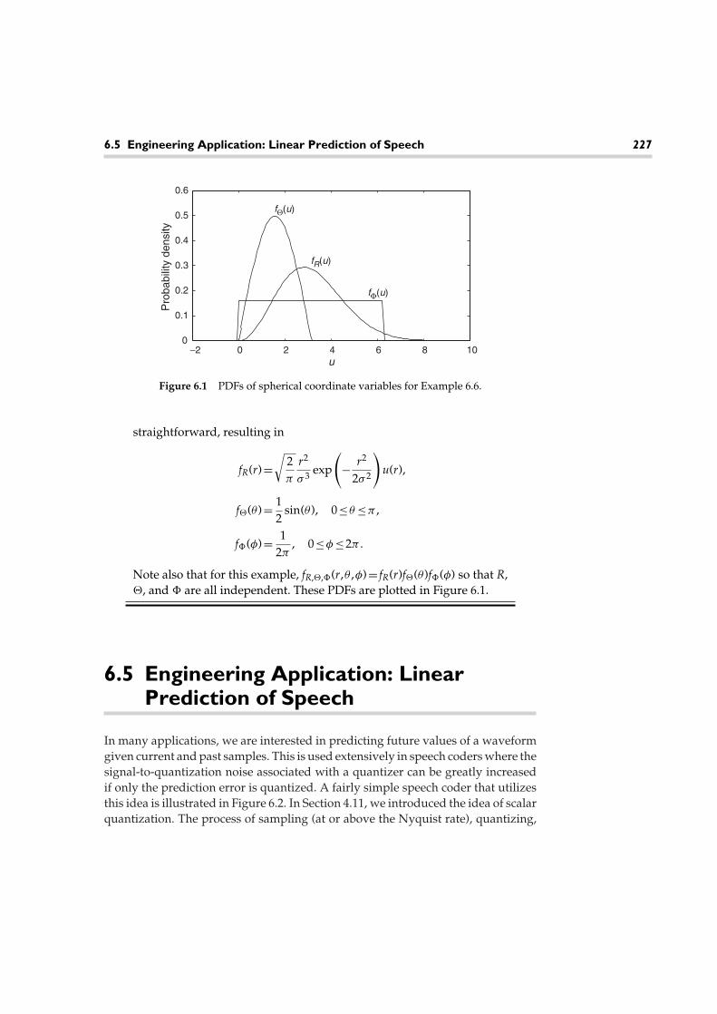
6.5 Engineering Application: Linear Prediction of Speech 227
−2 0 2 4 6 8 100
0.1
0.2
0.3
0.4
0.5
0.6
fΘ(u)
Pro
babi
lity
dens
ity
u
fR(u)
fΦ(u)
Figure 6.1 PDFs of spherical coordinate variables for Example 6.6.
straightforward, resulting in
fR(r)=√
2π
r2
σ 3 exp
(− r2
2σ 2
)u(r),
f(θ )= 12
sin(θ ), 0≤θ ≤π ,
f�(φ)= 12π
, 0≤φ ≤2π .
Note also that for this example, fR,,�(r,θ ,φ)= fR(r)f(θ )f�(φ) so that R,, and � are all independent. These PDFs are plotted in Figure 6.1.
6.5 Engineering Application: LinearPrediction of Speech
In many applications, we are interested in predicting future values of a waveformgiven current and past samples. This is used extensively in speech coders where thesignal-to-quantization noise associated with a quantizer can be greatly increasedif only the prediction error is quantized. A fairly simple speech coder that utilizesthis idea is illustrated in Figure 6.2. In Section 4.11, we introduced the idea of scalarquantization. The process of sampling (at or above the Nyquist rate), quantizing,

228 Chapter 6 Multiple Random Variables
+
Predictor
Quantizer Encoder+ −
XnBinarydataoutput
Zn Qn
Yn
Figure 6.2 Block diagram of a simple speech coder using differential pulse codemodulation.
and then encoding each quantization level with some binary code word is knownas pulse code modulation (PCM). In Figure 6.2, we consider a slight modification tothe basic PCM technique known as differential PCM (or DPCM). The basic idea hereis that if we can reduce the range of the signal that is being quantized, then wecan either reduce the number of quantization levels needed (and hence reduce thebit rate of the speech coder) or reduce the amount of quantization noise and henceincrease the SQNR.
A typical speech signal has a frequency content in the range from about 300–3500 Hz. In order to be able to recover the signal from its samples, a typical samplingrate of 8 KHz is used, which is slightly higher than the Nyquist rate. However, mostof the energy content of a speech signal is below 1 kHz; hence when sampled at8 kHz, a great deal of the speech signal does not change substantially from onesample to the next. Stated another way, when the speech signal is sampled at 8kHz, we should be able to predict future sample values from current and pastsamples with pretty good accuracy. The DPCM encoder does exactly that and thenonly quantizes and encodes the portion of the signal that it is not able to predict.
In Figure 6.2, the Xn represent samples of a speech waveform. These sam-ples are input to the predictor whose job is to make its best estimate of Xn givenXn−1,Xn−2,Xn−3, . . . as inputs. It is common to use linear prediction, in which casethe predictor output is a linear combination of the inputs. That is, assuming thepredictor uses the last m samples to form its estimate, the predictor output is of theform
Yn =m∑
i=1
aiXn−i, (6.59)
where the ai are constants that we select to optimize the performance of the pre-dictor. The quantity Zn =Xn−Yn is the predictor error, which we want to makeas small as possible. This error is quantized with a scalar quantizer that uses 2b
levels, and each level is encoded with a b bit code word. The overall bit rate of thespeech coder is b∗fs bits/second, where fs is the rate (in Hz) at which the speechis sampled. For example, if a 16-level quantizer were used with a speech samplingrate of 8 kHz, the DPCM speech coder would have a bit rate of 32 kbits/second.

6.5 Engineering Application: Linear Prediction of Speech 229
An important question is, Can the original samples be recovered from the binaryrepresentation of the signal? Given the encoded bit stream, we can construct thesequence of quantizer outputs, Qn. As with any quantization scheme, we can neverrecover the exact quantizer input from the quantizer output, but if we use enoughlevels in the quantizer, the quantization noise can be kept fairly small. The speechsamples are reconstructed according to Xn =Yn+Zn. Since we don’t have Zn, weuse Qn in its place and form
Xn =Yn+Qn =Xn+εn, (6.60)
where ε=Qn−Zn is the quantization noise in the nth sample. To complete theprocess of recovering the sample values, the decoder must also form the Yn. It cando this by employing an identical predictor as used at the encoder. Unfortunately,the predictor at the decoder does not have access to the same input as the predictorat the encoder. That is, at the decoder, we cannot use the true values of the pastspeech samples, but rather must use the quantized (noisy) versions. This can beproblematic since the predictor at the decoder will now form
Y =m∑
i=1
aiXn−1. (6.61)
If the Xn are noisy versions of the Xn, then the Yn will also be noisy. Now, notonly do we have quantization noise, but that noise propagates from one sampleto the next through the predictor. This leads to the possibility of a snowballingeffect, where the noise in our recovered samples gets progressively larger fromone sample to the next.
This problem is circumvented using the modified DPCM encoder shown inFigure 6.3; the corresponding decoder is shown in the figure as well. The differencebetween this DPCM system and the one in Figure 6.2 is that now the predictor usedin the encoder bases its predictions on the quantized samples rather than on thetrue samples. By doing this, the predicted value may be slightly degraded (butnot much if the number of quantization levels is sufficient), but there will be nopropagation of errors in the decoder, since the predictor at the decoder now usesthe same inputs as the predictor at the encoder.
Now that we have the design of the speech encoder and decoder squared away,we shift our attention to the problem of designing the predictor. Assuming a linearpredictor, the problem is essentially to choose the coefficients ai in Equation 6.59to minimize the prediction error:
Zn =Xn−Yn =Xn−m∑
i=1
aiXn−i. (6.62)

230 Chapter 6 Multiple Random Variables
+
Predictor
Quantizer Encoder+
−
Xn
DPCM encoder
+
Predictor
Decoder+
Binarydatainput
DPCM decoder
+
Zn QnBinarydataoutput
Qn
Yn
Xn
Yn
Figure 6.3 Block diagram of a modified speech coder using differential pulse codemodulation.
In this example, we choose to minimize the second moment of the error:
E[Z2n]=E
[(Xn−
m∑i=1
aiXn−i
)2]
. (6.63)
Differentiating the preceding expression with respect to aj and setting it equal tozero provides the following set of equations that the predictor coefficients shouldsatisfy:
m∑i=1
aiE[Xn−iXn−j]=E[XnXn−j], j=1,2, . . . ,m. (6.64)
Define the correlation parameter rk to be the correlation between two samplesspaced by k sampling intervals. Then our system of equations can be expressed inmatrix form as
r0 r1 r2 . . . rm−1r1 r0 r1 . . . rm−2r2 r1 r0 . . . rm−3. . . . . . . . . . . .
rm−1 rm−2 rm−3 . . . r0
=
a1a2a3. . .am
=
r1r2r3. . .rm
. (6.65)

6.5 Engineering Application: Linear Prediction of Speech 231
0 0.5 1 1.5 2 –1
–0.8
–0.6
–0.4
–0.2
0
0.2
0.4
0.6
0.8
1
time (seconds)
X(t
)
Figure 6.4 Speech segment used in Example 6.7.
EXAMPLE 6.7: Figure 6.4 shows a segment of speech that has a dura-tion of about 2 seconds, which was sampled at a rate of 8kHz. From thisdata, (using MATLAB) we estimated the correlation parameters rk =E[XnXn+k]; found the linear prediction coefficients, ai, i=1,2, . . . ,m; andthen calculated the mean squared estimation error, MSE=E[Xn−Yn)2].The results are shown in Table 6.1. We should note a couple of observa-tions. First, even with a simple one-tap predictor, the size of the errorsignal is much smaller than the original signal (compare the values ofMSE with r0 in the table). Second, we note that (for this example) theredoes not seem to be much benefit gained from using more than twoprevious samples to form the predictor.
Finally, we compare the quality of the encoded speech as measuredby the SQNR for PCM and the DPCM scheme of Figure 6.3 using thetwo-tap predictor specified in Table 6.1. For an equal number of bits persample, the DPCM scheme improves the SQNR by more than 20 dB.Alternatively, the DPCM scheme can use 3 bits/sample fewer than thePCM scheme and still provide better SQNR.
Note that the SQNR is an objective measure of speech quality and ispoorly correlated with speech quality. For example, one can introducea time delay to the estimated signal and obtain a very low SQNR value,yet the speech quality will be good.

232 Chapter 6 Multiple Random Variables
Table 6.1 Results of Linear Prediction of Speech Segment from Figure 6.4
r0 =0.0591 r1 =0.0568 r2 =0.0514 r3 =0.0442 r4 =0.0360
m=1 a1 =0.9615 MSE = 0.004473m=2 a1 =1.6564 a2 =−0.7228 MSE = 0.002144m=3 a1 =1.7166 a2 =−0.8492 a3 =0.0763 MSE = 0.002132m=4 a1 =1.7272 a2 =−1.0235 a3 =0.4276 a4 =−0.2052 MSE = 0.002044
1 2 3 4 5 6 7 8−10
0
10
20
30
40
50
60
70
Number of bits per sample
SQ
NR
DPCMPCM
Figure 6.5 SQNR comparison of PCM and DPCM speech coders for the speech segmentin Figure 6.4.
Exercises6.1 Suppose we flip a coin three times, thereby forming a sequence of heads
and tails. Form a random vector by mapping each outcome in the sequenceto 0 if a head occurs or to 1 if a tail occurs.
(a) How many realizations of the vector may be generated? List them.(b) Are the realizations independent of one another?
6.2 Let X=[X1,X2,X3]T represent a three-dimensional vector of randomvariables that is uniformly distributed over the unit sphere. That is,
fX(x)={
c ||x||≤10 ||x||>1
.

Exercises 233
(a) Find the constant c.(b) Find the marginal PDF for a subset of two of the three random variables.
For example, find fX1,X2 (x1,x2).(c) Find the marginal PDF for one of the three random variables. That is,
find fX1 (x1).(d) Find the conditional PDFs fX1|X2,X3 (x1|x2,x3) and fX1,X2|X3 (x1,x2|x3).
Extra: Can you extend this problem to N-dimensions?
6.3 Let X=[X1,X2, . . .XN]T represent an N-dimensional vector of random vari-ables that is uniformly distributed over the region x1+x2+···+xN ≤1,xi ≥0, i=1,2, . . . ,N. That is,
fX(x)={
c∑N
i=1 xi ≤1,xi ≥0
0 otherwise.
(a) Find the constant c.(b) Find the marginal PDF for a subset of M of the N random variables.(c) Are the Xi independent? Are the Xi identically distributed?
6.4 Consider a vector of N random variables, X=[X1,X2, . . . ,XN]T . Supposewe form a new random variable Z by performing a weighted average ofthe components of X. That is,
Z=N∑
i=1
biXi, where bi ≥0 andN∑
i=1
bi =1.
Find the values of the constants bi such that the variance of Z is minimized.
6.5 Show that all correlation matrices are nonnegative definite.
6.6 A random vector is generated by rolling a die and observing the outcome.The components of the random vector are determined by successive rollsof the die. If the die is rolled two times:
(a) list the possible realizations of the random vector;(b) determine the probability of each realization;(c) determine the mean vector;(d) determine the covariance matrix.
6.7 Repeat parts (c) and (d) of Exercise 6.6 if a three-element vector is formedfrom three rolls of a die.

234 Chapter 6 Multiple Random Variables
6.8 Let X be a two-element, zero-mean random vector. Suppose we constructa new random vector Y according to a linear transformation, Y=TX. Findthe transformation matrix, T, such that Y has a covariance matrix of
C=[
5 11 2
].
6.9 A three-dimensional vector random variable, X, has a covariance matrix of
C= 3 1 −1
1 5 −1−1 −1 3
.
Find a transformation matrix A, such that the new random variables Y=AXwill be uncorrelated.
6.10 Let X1, X2, and X3 be a set of three zero-mean Gaussian random variableswith a covariance matrix of the form
C=σ 2
1 ρ ρ
ρ 1 ρ
ρ ρ 1
.
Find the following expected values:
(a) E[X1|X2 =x2,X3 =x3],(b) E[X1X2|X3 =x3],(c) E[X1X2X3].
6.11 Define the N-dimensional characteristic function for a random vector X=[X1,X2, . . . ,XN]T , according to �X(�)=E[ej�T X] where �=[ω1,ω2, . . . ,ωN]T .Show that the N-dimensional characteristic function for a zero-meanGaussian random vector is given by
�X(�)=exp
(−�TCXX�
2
).
6.12 For any four zero-mean Gaussian random variables X1,X2,X3, and X4,show that
E[X1X2X3X4]=E[X1X2]E[X3X4]+E[X1X3]E[X2X4]+E[X1X4]E[X2X3].
Hint: You might want to use the result of Exercise 6.11.

Exercises 235
6.13 Suppose Xm, m=1,2, . . . ,n are a sequence of independent and exponentiallydistributed random variables with
fXm (x)= 1µ
exp(−x/µ)u(x).
Assume that n is an odd number (n=2k−1 for some integer k).
(a) Find the PDF of the median of the sequence.(b) Find the expected value of the median of the sequence. Is the median
an unbiased estimate of the mean of the underlying exponentialdistribution?
(c) Find the variance of the median of the sequence.
6.14 Show that the derivative of
FYm (y)=N∑
k=m
(Nk
)(FX(y))k(1−FX(y))N−k
reduces to the form
fYm (y)= N!(m−1)!(N−m)! fX(y)(FX(y))m−1(1−FX(y))N−m.
6.15 In this problem we formulate an alternative derivation of Equation 6.58that gives the PDF of the order statistic, Ym, which is the mth largest of asequence of N random variables, X1,X2, . . . ,XN . Start by writing fYm (y)dy =Pr(y <Ym <y+dy). Then note that
Pr(y <Ym <y+dy)=Pr({m−1 of the Xs are less than y}∩{1 X is between y and y+dy}∩{n−m of the Xs are greater than y}).
Find the probability of this event and by doing so, prove that the PDF ofYm is as given by Equation 6.58.
6.16 The traffic managers of toll roads and toll bridges need specific informationto properly staff the toll booths so that the queues are minimized (i.e., thewaiting time is minimized).
(a) Assume that there is one toll booth on a busy interstate highway andthat the number of cars per minute approaching the toll booth follows aPoisson PMF with α=10. The traffic manager wants you to determinethe probability that exactly 11 cars will approach this toll booth in theminute from noon to one minute past noon.

236 Chapter 6 Multiple Random Variables
(b) Now assume there are N toll booths at a toll plaza and that the num-ber of cars per minute approaching the plaza follows a Poisson PMFwith α=30. The traffic manager wants you to calculate the minimumnumber of toll booths that need to be staffed if the probability is atleast 0.05 that not more than five cars approach each toll booth in oneminute. For this part, assume the traffic approaching the plaza dividesitself among the N booths such that the traffic approaching each boothis independent and follows a Poisson PMF with α=30/N.
6.17 A sequence of zero mean unit variance independent random variables, Xn,n=0,1,2, . . . ,N−1 are input to a filter that produces an output sequenceaccording to Yn = (Xn+Xn−1)/2 for n=0,1,2, . . . ,N−1. For initializationpurposes, X−1 is taken to be zero.
(a) Find the covariance (correlation) matrix of the Yn.(b) Now let the variance of the Xn be σ 2
X . Find the covariance (correlation)matrix of the Yn.
6.18 Repeat Exercise 6.17 with the filter changed to Yn =Xn−Xn−1.
6.19 Suppose a zero-mean random sequence Xn has correlation parametersgiven by rk =E[XnXn+k]= c|k|. An estimate of a future value of Xn isXn =a1Xn−1+a2Xn−2, which is a special case of Equation 6.59.
(a) Use Equation 6.65 to find the ai.(b) What is the mean squared error, E[(Xn−Xn)2]?
MATLAB Exercises6.20 Three jointly Gaussian random variables [X,Y,Z]T have a mean vector
µ=[1,0,−1]T and covariance matrix
C= 4 2 −1
2 4 2−1 2 4
.
Use MATLAB to help you find the form of the three-dimensional joint PDF,fX,Y,Z(x,y,z).
6.21 For each of the following matrices, determine if the matrix is a valid cor-relation matrix. In some cases, you may want to use MATLAB to check ifthe matrix is positive definite.

MATLAB Exercises 237
(a) Ca = 3 −2 1
2 6 0−1 0 2
, (b) Cb =
3 −2 3
−2 6 03 0 2
,
(c) Cc = 3 −2 1
−2 6 01 0 2
, (d) Cd =
1 −12
14
−18
−12
1 −12
14
14
−12
1 −12
−18
14
−12
1
,
(e) Ce =
11 −3 7 5−3 11 5 77 5 11 −35 7 −3 11
, (f) Cf =
5 1 3 −11 5 −1 33 −1 5 1
−1 3 1 5
.
6.22 For each matrix in the previous problem that is a valid correlation matrix,find a transformation matrix that will transform a set of independent unitvariance random variables into a set of random variables with the specifiedcorrelation matrix.
6.23 Given a random sequence X=[X1,X2,X3,X4] with a covariance matrix
CX =
1 0.3 0.09 0.0270.3 1 0.3 0.027
0.09 0.3 1 0.30.0027 0.09 0.3 1
,
find a linear transformation that will produce a random sequence Y=[Y1,Y2,Y3,Y4] with a covariance matrix
CY =
1 0.1 0.2 0.30.1 1 0.1 0.20.2 0.1 1 0.10.3 0.2 0.1 1
.

Random Sequences andSeries 7
This chapter forms a bridge between the study of random variables in the previouschapters and the study of random processes to follow. A random process is simplya random function of time. If time is discrete, then such a random function couldbe viewed as a sequence of random variables. Even when time is continuous, weoften choose to sample waveforms (whether they are deterministic or random) inorder to work with discrete time sequences rather than continuous time waveforms.Hence, sequences of random variables will naturally occur in the study of randomprocesses. In this chapter, we’ll develop some basic results regarding both finiteand infinite sequences of random variables and random series.
7.1 Independent and IdenticallyDistributed Random Variables
In many applications, we are able to observe an experiment repeatedly. Each newobservation can occur with an independent realization of whatever random phe-nomena control the experiment. This sort of situation gives rise to independent andidentically distributed (i.i.d. or IID) random variables.
DEFINITION 7.1: A sequence of random variables X1, X2, . . . , Xn is IID if
FXi (x) = FX(x) ∀ i = 1, 2, . . . , n (identically distributed), (7.1)
239

240 Chapter 7 Random Sequences and Series
and
FX1, X2, ... ,Xn (x1, x2, . . . , xn) =n∏
i=1
FXi (xi) (independent). (7.2)
For continuous random variables, the CDFs can be replaced with PDFs inEquations 7.1 and 7.2, while for discrete random variables the CDFs can be replacedby PMFs.
Suppose, for example, we wish to measure the voltage produced by a certainsensor. The sensor might be measuring the relative humidity outside. Our sensorconverts the humidity to a voltage level that we can then easily measure. However,as with any measuring equipment, the voltage we measure is random due to noisegenerated in the sensor as well as in the measuring equipment. Suppose the voltagewe measure is represented by a random variable X given by X = v(h) + N, wherev(h) is the true voltage that should be presented by the sensor when the humidityis h, and N is the noise in the measurement. Assuming that the noise is zero-mean,then E[X] = v(h). That is, on the average, the measurement will be equal to thetrue voltage v(h). Furthermore, if the variance of the noise is sufficiently small,then the measurement will tend to be close to the true value we are trying tomeasure. But what if the variance is not small? Then the noise will tend to distortour measurement making our system unreliable. In such a case, we might be ableto improve our measurement system by taking several measurements. This willallow us to “average out” the effects of the noise.
Suppose we have the ability to make several measurements and observe asequence of measurements X1, X2, . . . , Xn. It might be reasonable to expect thatthe noise that corrupts a given measurement has the same distribution each time(and hence the Xi are identically distributed) and is independent of the noise inany other measurement (so that the Xi are independent). Then the n measurementsform a sequence of IID random variables. A fundamental question is then How dowe process an IID sequence to extract the desired information from it? In the pre-ceding case above, the parameter of interest, v(h), happens to be the mean of thedistribution of the Xi. This turns out to be a fairly common problem, so we start byexamining in some detail the problem of estimating the mean from a sequence ofIID random variables.
7.1.1 Estimating the Mean of IID Random Variables
Suppose the Xi have some common PDF, fX(x), which has some mean value, µX .Given a set of IID observations, we wish to form some function
µ = g(X1, X2, . . . , Xn), (7.3)

7.1 Independent and Identically Distributed Random Variables 241
which will serve as an estimate of the mean. But what function should we choose?Even more fundamentally, what criterion should we use to select a function?
There are many criteria that are commonly used. To start with, we would likethe average value of the estimate of the mean to be equal to the true mean. That is,we want E[µ] = µX . If this criterion is met, we say that µ is an unbiased estimate ofµX . Given that the estimate is unbiased, we would also like the error in the estimateto be as small as possible. Define the estimation error to be ε = µ−µX . A commoncriterion is to choose the estimator that minimizes the second moment of the error(mean-square error), E
[ε2] = E
[(µ − µX)2]. If this criterion is met, we say that µ
is an efficient estimator of µX . To start with a relatively simple approach, supposewe desire to find a linear estimator. That is, we will limit ourselves to estimatorsof the form
µ = a1X1 + a2X2 + · · · + anXn =n∑
i=1
aiXi. (7.4)
Then, we seek to find the constants a1, a2, . . . , an such that the estimator (1) is unbi-ased and (2) minimizes the mean-square error. Such an estimator is referred to asthe best linear unbiased estimator (BLUE).
To simplify notation in this problem, we write X = [X1, X2, . . . , Xn]T and a =[a1, a2, . . . , an]T . The linear estimator µ can then be written as µ = aTX. First, forthe estimator to be unbiased, we need
µX = E[µ] = E[aTX
] = aTE[X]. (7.5)
Since the Xi are all IID, they all have means equal to µX . Hence, the mean vectorfor X is just µX1n, where 1n is an n-element column vector of all 1s. The linearestimator will then be unbiased if
n∑
i=1
ai = aT1n = 1. (7.6)
The mean square error is given by
E[ε2] = E
[(aTX − µX
)2] = aTE[XXT]a − 2µXaTE[X] + µ2
X
= aTRa − 2µ2XaT1n + µ2
X . (7.7)
In this expression, R = E[XXT ] is the correlation matrix for the vector X. Using theconstraint of Equation 7.6, the mean square error simplifies to
E[ε2] = aTRa − µ2X . (7.8)
The problem then reduces to minimizing the function aTRa subject to the constraintaT1n = 1.

242 Chapter 7 Random Sequences and Series
To solve this multidimensional optimization problem, we use standardLagrange multiplier techniques. Form the auxiliary function
h(λ) = aTRa + λaT1n. (7.9)
Then solve the equation ∇h = 0. It is not difficult to show that the gradient of thefunction h works out to be ∇h = 2Ra + λ1n. Hence, the optimum vector a willsatisfy
Ra =(
−λ
2
)1n. (7.10)
Solving for a in this equation and then applying the constraint aT1n = 1 results inthe solution
a = R−11n
1Tn R−11n
. (7.11)
Due to the fact that the Xi are IID, the form of the correlation matrix can easilybe shown to be
R = µ2X1nxn + σ 2
XI, (7.12)
where 1nxn is an nxn matrix consisting of all 1s and I is an identity matrix. Also,σ 2
X is the variance of the IID random variables. It can be shown using the matrixinversion lemma1 that the inverse of this correlation matrix is
R−1 = σ−2X
[I − µ2
X/σ 2X
1 + nµ2X/σ 2
X
1nxn
]. (7.13)
From here, it is easy to demonstrate that R−11n is proportional to 1n, and hence theresulting vector of optimum coefficients is
a = 1n
1n. (7.14)
In terms of the estimator µ, the best linear unbiased estimator of the mean of anIID sequence is
µ = 1n
1Tn X = 1
n
n∑
i=1
Xi. (7.15)
1The matrix inversion lemma gives a formula to find the inverse of a rank one update ofanother matrix whose inverse is known. In particular, suppose A = B + xxT , where x is acolumn vector and the inverse of B is known. Then
A−1 = B−1 − B−1xxT B−1
1 + xT B−1x.

7.1 Independent and Identically Distributed Random Variables 243
This estimator is commonly referred to as the sample mean. The preceding derivationproves Theorem 7.1, which follows.
THEOREM 7.1: Given a sequence of IID random variables X1, X2, . . . , Xn, thesample mean is BLUE.
Another common approach to estimate various parameters of a distribution isthe maximum likelihood (ML) approach. In the ML approach, the distribution parame-ters are chosen to maximize the probability of the observed sample values. Suppose,as in the preceding discussion, we are interested in estimating the mean of a distri-bution. Given a set of observations, X1 = x1, X2 = x2, . . . , Xn = xn, the ML estimateof µX would be the value of µX that maximizes fX(x). A few examples will clarifythis concept.
EXAMPLE 7.1: Suppose the Xi are jointly Gaussian so that
fX(x) = 1(2πσ 2)n/2
exp
(− 1
2σ 2
n∑
i=1
(xi − µ)2
).
The value of µ that maximizes this expression will minimizen∑
i=1
(xi − µ)2.
Differentiating and setting equal to zero gives the equation
−2n∑
i=1
(xi − µ) = 0.
The solution to this equation works out to be
µML = 1n
n∑
i=1
xi.
Hence, the sample mean is also the ML estimate of the mean when therandom variables follow a Gaussian distribution.
EXAMPLE 7.2: Now suppose the random variables have an exponen-tial distribution,
fX(x) =n∏
i=1
1µ
exp(
−xi
µ
)u(xi) = 1
µn exp
(− 1
µ
n∑
i=1
xi
) n∏
i=1
u(xi).
244 Chapter 7 Random Sequences and Series
Differentiating with respect to µ and setting equal to zero results in
− nµn+1 exp
(− 1
µ
n∑
i=1
xi
)+ 1
µ2
( n∑
i=1
xi
)1µn exp
(− 1
µ
n∑
i=1
xi
)= 0.
Solving for µ results in
µML = 1n
n∑
i=1
xi.
Once again, the sample mean is the maximum likelihood estimate of themean of the distribution.
Since the sample mean occurs so frequently, it is beneficial to study this esti-mator in a little more detail. First, we note that the sample mean is itself a randomvariable since it is a function of the n IID random variables. We have already seenthat the sample mean is an unbiased estimate of the true mean; that is, E[µ] = µX .It is instructive also to look at the variance of this random variable.
Var(µ) = E
(
1n
n∑
i=1
Xi − µX
)2
= E
(
1n
n∑
i=1
(Xi − µX)
)2
= 1n2
n∑
i=1
n∑
j=1
E[(Xi − µX)(Xj − µX)]
= 1n2
n∑
i=1
n∑
j=1
E[(Xi − µX)(Xj − µX)] = 1n2
n∑
i=1
n∑
j=1
Cov(Xi, Xj) (7.16)
All terms in the double series in the previous equation are zero except for the oneswhere i = j since Xi and Xj are uncorrelated for all i �= j. Hence, the variance of thesample mean is
Var(µ) = 1n2
n∑
i=1
Var(Xi) = 1n2
n∑
i=1
σ 2X = σ 2
Xn
. (7.17)
This means that if we use n samples to estimate the mean, the variance of theresulting estimate is reduced by a factor of n relative to what the variance wouldbe if we used only one sample.
Consider what happens in the limit as n → ∞. As long as the variance of each ofthe samples is finite, the variance of the sample mean approaches zero. Of course,we never have an infinite number of samples in practice, but this does mean that

7.1 Independent and Identically Distributed Random Variables 245
the sample mean can achieve any level of precision (i.e., arbitrarily small variance)if a sufficient number of samples is taken. We will study this limiting behaviorin more detail in section 7.3. For now, we turn our attention to estimating otherparameters of a distribution.
7.1.2 Estimating the Variance of IID RandomVariables
Now that we have a handle on how to estimate the mean of IID random variables,suppose we would like also to estimate the variance (or equivalently, the standarddeviation). Since the variance is not a linear function of the random variables, itwould not make much sense to try to form a linear estimator. That is, to talk aboutan estimator of the variance being BLUE does not make much sense. Hence, wetake the ML approach here. As with the problem of estimating the mean, we seekthe value of the variance that maximizes the joint PDF of the IID random variablesevaluated at their observed values.
EXAMPLE 7.3: Suppose that the random variables are jointly Gaussianso that
fX(x) = 1(2πσ 2)n/2
exp
(− 1
2σ 2
n∑
i=1
(xi − µ)2
).
Differentiating the joint PDF with respect to σ results in
ddσ
fX(x)=(
− nσ
+ 1σ 3
n∑
i=1
(xi−µ)2
)1
(2πσ 2)n/2exp
(− 1
2σ 2
n∑
i=1
(xi−µ)2
).
Setting this expression equal to zero and solving results in
σ 2ML = 1
n
n∑
i=1
(xi − µ)2.
The result of Example 7.3 seems to make sense. The only problem with thisestimate is that it requires knowledge of the mean in order to form the estimate.What if we don’t know the mean? One obvious approach would be to replace thetrue mean in the previous result with the sample mean. That is, one could estimate
246 Chapter 7 Random Sequences and Series
the variance of an IID sequence using
s2 = 1n
n∑
i=1
(xi − µ)2, µ = 1n
n∑
i=1
xi. (7.18)
This approach, however, can lead to problems. It is left as an exercise for the readerto show that this estimator is biased; that is, in this case, E[σ 2] �= σ 2. To overcomethis problem, it is common to adjust the previous form. The following estimatorturns out to be an unbiased estimate of the variance:
s2 = 1n − 1
n∑
i=1
(xi − µ)2. (7.19)
This is known as the sample variance and is the most commonly used estimate forthe variance of IID random variables. In the previous expression, µ is the usualsample mean.
In summary, given a set of IID random variables, the variance of the distributionis estimated according to
s2 =
1n
n∑
i=1
(xi − µ)2 if µ is known
1n − 1
n∑
i=1
(xi − µ)2 if µ is unknown
(7.20)
EXAMPLE 7.4: Suppose we form a random variable Z accord-ing to Z =
√X2 + Y2 where X and Y are independent Gaussian
random variables with means of µ and variances of σ 2. In thisexample, we will estimate the mean and variance of Z using the
sample mean and sample variance of a large number of MATLAB-generatedrealizations of the random variable Z. The MATLAB code to accomplish thisfollows. Upon running this code, we obtain a sample mean of µ = 5. 6336 anda sample variance of s2 = 8. 5029. Note that the true mean and variance of theRician random variable Z can be found analytically (with some effort). Forthis example, the PDF of the random variable Z is found to take on a Ricianform
fZ(z) = zσ 2 exp
(−z2 + 2µ2
2σ 2
)I0
(√2µzσ 2
)u(z).

7.1 Independent and Identically Distributed Random Variables 247
Using the expressions given in Appendix D, Summary of Common RandomVariables (see Equations D.52 and D.53), for the mean and variance of a Ricianrandom variable, it is determined that the true mean and variance should be
µZ =√
πσ 2
2exp
(− µ2
2σ 2
)[(1 + µ2
σ 2
)Io
(µ2
2σ 2
)+ µ2
σ 2 I1
(µ2
2σ 2
)],
σ 2Z = 2σ 2 + 2µ2 − µ2
Z.
For the values of µ = 2 and σ = 4 used in the following program, the resultingmean and variance of the Rician random variable should be µZ = 5. 6211 andσ 2
Z = 8. 4031.
N=10000;
mu=2; sigma=4; % Set mean and standard
deviation of X and Y.
X=sigma*randn(1,N)+mu; % Generate samples of X.
Y=sigma*randn(1,N)+mu; % Generate samples of Y.
Z=sqrt(X.∧2+Y.∧2); % Create Z (Rician RVs).
mu_hat=sum(Z)/N % Sample mean.
s_hat2=sum((Z-mu_hat).∧2)/(N-1) % Sample variance.
7.1.3 Estimating the CDF of IID Random Variables
Suppose instead of estimating the parameters of a distribution, we were interestedin estimating the distribution itself. This can be done using some of the previousresults. The CDF of the underlying distribution is FX(x) = Pr(X ≤ x). For anyspecific value of x, define a set of related variables Y1, Y2, . . . , Yn such that
Yi ={
1 if Xi ≤ x
0 if Xi > x. (7.21)
It should be fairly evident that if the Xi are IID, then the Yi must be IID as well.Note that for these Bernoulli random variables, the mean is E[Yi] = Pr(Xi ≤ x).Hence, estimating the CDF of the Xi is equivalent to estimating the mean of the Yi,which is done using the sample mean:
FX(x) = 1n
n∑
i=1
Yi = 1n
n∑
i=1
[1 − u(Xi − x)]. (7.22)

248 Chapter 7 Random Sequences and Series
This estimator is nothing more than the relative frequency interpretation of prob-ability. To estimate FX(x) from a sequence of n IID observations, we merely countthe number of observations that satisfy Xi ≤ x.
EXAMPLE 7.5: To illustrate this procedure of estimating the CDFof IID random variables, suppose the Xi are all uniformly dis-tributed over (0, 1). The plot in Figure 7.1 shows the results of onerealization of estimating this CDF using n IID random variables
for n = 10, n = 100, and n = 1000. Clearly, as n gets larger, the estimate getsbetter. The MATLAB code that follows can be used to generate a plot similarto the one in the figure. The reader is encouraged to try different types ofrandom variables in this program as well.
N=100; % Set number of samples.
z=[-0.5:0.01:1.5]; % Define variable for horizontal axis.
x=rand(1,N); % Generate uniform random samples.
F=zeros(1,length(z)); % Initialize CDF estimate.
for n=1:N % Estimate CDF.
F=F+(x(n)<z);
end
−0.5 0 0.5 1 1.50
0.1
0.2
0.3
0.4
0.5
0.6
0.7
0.8
0.9
1
FX(x
)
x
n=10 n=100 n=1000
Figure 7.1 Estimate of the CDF of a uniform random variable obtained from n IID randomvariables, n = 10, 100, and 1000.

7.2 Convergence Modes of Random Sequences 249
F=F/N;
plot(z,F) % Plot results.
xlabel(‘x’); ylabel(‘F_X(x)’)
7.2 Convergence Modes of RandomSequences
In many engineering applications, it is common to use various iterative procedures.In such cases, it is often important to know under what circumstances an iterativealgorithm converges to the desired result. The reader is no doubt familiar withmany such applications in the deterministic world. For example, suppose we wishto solve for the root of some equation g(x) = 0. One could do this with a variety ofiterative algorithms (e.g., Newton’s method). The convergence of these algorithmsis a quite important topic. That is, suppose xi is the estimate of the root at the ithiteration of Newton’s method. Does the sequence x1, x2, x3, . . . converge to the trueroot of the equation? In this section, we study the topic of random sequences andin particular the issue of convergence of random sequences.
As an example of a random sequence, suppose we started with a set of IIDrandom variables, X1, X2, . . . , Xn, and then formed the sample mean according to
Sn = 1n
n∑
i=1
Xi. (7.23)
The sequence S1, S2, S3, . . . is a sequence of random variables. It is desirable that thissequence converge to the true mean of the underlying distribution. An estimatorsatisfying this condition is called consistent. But in what sense can we say that thesequence converges? If a sequence of deterministic numbers s1, s2, s3, . . . were beingconsidered, the sequence would be convergent to a fixed value s if
limi→∞
si = s. (7.24)
More specifically, if for any ε > 0, there exists an iε such that |si − s| < ε for alli > iε, then the sequence is said to converge to s.
Suppose an experiment, E, is run resulting in a realization, ζ . Each realization ismapped to a particular sequence of numbers. For example, the experiment mightbe to observe a sequence of IID random variables X1, X2, X3, . . . and then mapthem into a sequence of sample means S1, S2, S3, . . .. Each realization, ζ , leads toa specific deterministic sequence, some of which might converge (in the previoussense) while others might not converge. Convergence for a sequence of randomvariables is not straightforward to define and can occur in a variety of manners.

250 Chapter 7 Random Sequences and Series
7.2.1 Convergence Everywhere
The first and strictest form of convergence is what is referred to as convergenceeverywhere (a.k.a. sure convergence). A sequence is said to converge everywhereif every realization, ζ , leads to a sequence, sn(ζ ), that converges to s(ζ ). Note thatthe limit may depend on the particular realization. That is, the limit of the randomsequence may be a random variable.
7.2.2 Convergence Almost Everywhere
In many examples, it may be possible to find one or several realizations of therandom sequence that do not converge, in which case the sequence (obviously) doesnot converge everywhere. However, it may be the case that such realizations areso rare that we might not want to concern ourselves with such cases. In particular,suppose that the only realizations that lead to a sequence that does not convergeoccur with probability zero. Then we say the random sequence converges almosteverywhere (a.k.a. almost sure convergence or convergence with probability 1).Mathematically, let A be the set of all realizations that lead to a convergent sequence.Then the sequence converges almost everywhere if Pr(A) = 1.
7.2.3 Convergence in Probability
A random sequence S1, S2, S3, . . . converges in probability to a random variable Sif for any ε > 0,
limn→∞ Pr
(∣∣Sn − S∣∣ > ε
) = 0. (7.25)
7.2.4 Convergence in the Mean Square (MS)Sense
A random sequence S1, S2, S3, . . . converges in the MS sense to a random vari-able S if
limn→∞ E
[∣∣Sn − S∣∣2]
= 0. (7.26)

7.3 The Law of Large Numbers 251
7.2.5 Convergence in Distribution
Suppose the sequence of random variables S1, S2, S3, . . . has CDFs given by FSn (s),and the random variable S has a CDF, FS(s). Then, the sequence converges indistribution if
limn→∞ FSn (s) = FS(s) (7.27)
for any s that is a point of continuity of FS(s).
7.3 The Law of Large Numbers
Having described the various ways in which a random sequence can converge, wereturn now to the study of sums of random variables. In particular, we look inmore detail at the sample mean. The following very well known result is knownas the weak law of large numbers.
THEOREM 7.2 (The Weak Law of Large Numbers): Let Sn be the sample meancomputed from n IID random variables, X1, X2, . . . , Xn. The sequence of sam-ple means, Sn, converges in probability to the true mean of the underlyingdistribution, FX(x).
PROOF: Recall that if the distribution FX(x) has a mean of µ and variance σ 2,then the sample mean, Sn, has mean µ and variance σ 2/n. Applying Chebyshev’sinequality,
Pr(∣∣Sn − µ
∣∣ > ε) ≤ Var(Sn)ε2 = σ 2
nε2 . (7.28)
Hence, limn→∞ Pr(∣∣Sn − µ
∣∣ > ε) = 0 for any ε > 0. Thus, the sample meanconverges in probability to the true mean. �
The implication of this result is that we can estimate the mean of a random variablewith any amount of precision with arbitrary probability if we use a sufficientlylarge number of samples. A stronger result known as the strong law of large numbersshows that the convergence of the sample mean is not just in probability but alsoalmost everywhere. We do not give a proof of this result in this text.
As was demonstrated in Section 7.2.3, the sample mean can be used to estimatemore than just means. Suppose we are interested in calculating the probability thatsome event A results from a given experiment. Assuming that the experiment isrepeatable and that each time the results of the experiment are independent of allother trials, then Pr(A) can easily be estimated. Simply define a random variable Xi

252 Chapter 7 Random Sequences and Series
that is an indicator function for the event A on the ith trial. That is, if the event Aoccurs on the ith trial, then Xi = 1; otherwise, Xi = 0. Then
Pr(A) = Pr(Xi = 1) = E[Xi]. (7.29)
The sample mean,
µn = 1n
n∑
i=1
Xi, (7.30)
will give an unbiased estimate of the true probability, Pr(A). Furthermore, the law oflarge numbers tells us that as the sample size gets large, the estimate will convergeto the true value. The weak law of large numbers tells us that the convergence isin probability while the strong law of large numbers tells us that the convergenceis also almost everywhere.
The technique we’ve described for estimating the probability of events is knownas the Monte Carlo simulation. It is commonly used, for example, to estimate thebit error probability of a digital communication system. A program is written tosimulate transmission and detection of data bits. After a large number of data bitshave been simulated, the number of errors is counted and divided by the totalnumber of bits transmitted. This gives an estimate of the true probability of biterror of the system. If a sufficiently large number of bits are simulated, arbitraryprecision of the estimate can be obtained.
EXAMPLE 7.6: This example shows how the sample mean andsample variance converge to the true mean for a few differentrandom variables. The results of running the MATLAB code thatfollows are shown in Figure 7.2. Plot (a) shows the results for a
Gaussian distribution, whereas plot (b) shows the same results for an arcsinerandom variable. In each case, the parameters have been set so that the truemean is µ = 3 and the variance of each sample is 1. Since the variance of thesample mean depends on only the variance and the number of the samples,crudely speaking the “speed” of convergence should be about the same inboth cases.
N=100;
% Create Gaussian random variables.mu1=3; sigma1=1;X1=sigma1*randn(1,N)+mu1;mu_hat1=cumsum(X1)./[1:N]; % sample means.
% Create Arcsine random variables.mu2=3; b=sqrt(2); sigma2=b∧2/2;

7.4 The Central Limit Theorem 253
0 10 20 30 40 50 60 70 80 90 1000
1
2
3
4
5
6
0 10 20 30 40 50 60 70 80 90 1000
1
2
3
4
5
6
Samples, n
Sam
ple
mea
n
Gaussian
Samples, n
Sam
ple
mea
n
Arcsine
(a)
(b)
Figure 7.2 Convergence of the sample mean for Gaussian (a) and Arcsine (b) randomvariables.
X2=b*cos(2*pi*rand(1,N))+mu2;
mu_hat2=cumsum(X2)./[1:N]; % sample means.
subplot(2,1,1)
plot([1:N],mu_hat1,‘-’,[1:N], mu1, ‘–’)
xlabel(‘n’); ylabel(‘S_n’); title(‘Gaussian’)
axis([0,N,0,2*mu1])
subplot(2,1,2)
plot([1:N],mu_hat2,‘-’,[1:N], mu2, ‘–’)
xlabel(‘n’); ylabel(‘S_n’); title(‘Arcsine’)
axis([0,N,0,2*mu2])
7.4 The Central Limit Theorem
Probably the most important result dealing with sums of random variables is thecentral limit theorem, which states that under some mild conditions, these sums

254 Chapter 7 Random Sequences and Series
converge to a Gaussian random variable in distribution. This result provides thebasis for many theoretical models of random phenomena. It also explains whythe Gaussian random variable is of such great importance and why it occurs sofrequently. In this section, we prove a simple version of the central limit theoremand then discuss some of the generalizations.
THEOREM 7.3 (The Central Limit Theorem): Let Xi be a sequence of IID randomvariables with mean µX and variance σ 2
X . Define a new random variable, Z, as asum of the Xi:
Z = 1√n
n∑
i=1
Xi − µX
σx. (7.31)
Note that Z has been constructed such that E[Z] = 0 and Var(Z) = 1. In the limitsas n approaches infinity, the random variable Z converges in distribution to astandard normal random variable.
PROOF: The most straightforward approach to prove this important theorem isusing characteristic functions. Define the random variable Xi as Xi = (Xi −µX)/σX .The characteristic function of Z is computed as
�Z(ω) = E[ejωZ] = E
[exp
(jω√
n
n∑
i=1
Xi
)]= E
[ n∏
i=1
exp
(jωXi√
n
)]
=n∏
i=1
E
[exp
(jωXi√
n
)]=
n∏
i=1
φX
(ω√n
)=[φX
(ω√n
)]n
. (7.32)
Next, recall Taylor’s theorem2, which states that any function g(x) can be expandedin a power series of the form
g(x) = g(xo) + dgdx
∣∣∣∣x=xo
(x − xo) + · · · + 1k!
dkgdxk
∣∣∣∣x=xo
(x − xo)k + rk(x, xo), (7.33)
where the remainder rk(x, xo) is small compared to (x − xo)k as x → xo. Applyingthe Taylor series expansion about the point ω = 0 to the characteristic function ofX results in
φX(ω) = φX(0) + φ′X
(0)ω + 12φ
′′X
(0)ω2 + r3(ω), (7.34)
2See, for example, Marsden, J. and A. Tromba, Vector Calculus, 5th ed., New York:W. H. Freeman, 2004.

7.4 The Central Limit Theorem 255
where r3(ω) is small compared to ω2 as ω → 0. Furthermore, we note that φX(0) = 1,φ
′X
(0) = jE[X] = 0, and φ′′X
(0) = −E[X2] = −1. Hence Equation 7.34 reduces to
φX(ω) = 1 − ω2
2+ r3(ω). (7.35)
The characteristic function of Z is then
�Z(ω) =(
1 − ω2
2n+ r3
(ω√n
))n
. (7.36)
Note that as n → ∞, the argument of r3( ) goes to zero for any finite ω. Hence, asn → ∞, r3(ω/
√n) becomes negligible compared to ω2/n. Therefore, in the limit,
the characteristic function of Z approaches3
limn→∞ �Z(ω) = lim
n→∞
(1 − ω2
2n
)n
= exp
(−ω2
2
). (7.37)
This is the characteristic function of a standard normal random variable. �
Several remarks about this theorem are in order at this point. First, no restric-tions were put on the distribution of the Xi. The preceding proof applies to anyinfinite sum of IID random variables, regardless of the distribution. Also, the cen-tral limit theorem guarantees that the sum converges in distribution to Gaussian,but this does not necessarily imply convergence in density. As a counterexample,suppose that the Xi are discrete random variables. Then the sum must also be a dis-crete random variable. Strictly speaking, the density of Z would then not exist andit would not be meaningful to say that the density of Z is Gaussian. From a prac-tical standpoint, the probability density of Z would be a series of impulses. Whilethe envelope of these impulses would have a Gaussian shape to it, the density isclearly not Gaussian. If the Xi are continuous random variables, the convergencein density generally occurs as well.
The proof of the central limit theorem just given assumes that the Xi are IID.This assumption is not needed in many cases. The central limit theorem also appliesto independent random variables that are not necessarily identically distributed.
3Here we have used the well-known fact that limn→∞(1 + (x/n))n = ex. To establish this
result, the interested reader is encouraged to expand both sides in a Taylor series and showthat in the limit the two expansions become equivalent.

256 Chapter 7 Random Sequences and Series
Loosely speaking4, all that is required is that no single term (or small number ofterms) dominate the sum and the resulting infinite sum of independent randomvariables will approach a Gaussian distribution in the limit as the number of termsin the sum goes to infinity. The central limit theorem also applies to some cases ofdependent random variables, but we will not consider such cases here.
From a practical standpoint, the central limit theorem implies that for thesum of a sufficiently large (but finite) number of random variables, the sum isapproximately Gaussian distributed. Of course, the goodness of this approximationdepends on how many terms are in the sum and also on the distribution of theindividual terms in the sum. The next examples show some illustrations to givethe reader a feel for the Gaussian approximation.
EXAMPLE 7.7: Suppose the Xi are all independent and uniformlydistributed over (−1/2, 1/2). Consider the sum
Z =√
12n
n∑
i=1
Xi.
The sum has been normalized so that Z has zero-mean and unit variance.It was shown previously that the PDF of the sum of independent randomvariables is just the convolution of the individual PDFs. Hence, if wedefine Y to be Y = X1 + X2 + · · · + Xn, then
fY(z) = fX(z) ∗ fX(z) ∗ · · · ∗ fX(z), and fZ(z) =√
n12
fY
(z√
n12
).
The results of performing this n-fold convolution are shown in Figure 7.3for several values of n. Note that for as few as n = 4 or n = 5 termsin the series, the resulting PDF of the sum looks very much like theGaussian PDF.
EXAMPLE 7.8: In this example, suppose the Xi are now discreteBernoulli distributed random variables such that Pr(Xi = 1) =Pr(Xi = 0) = 0. 5. In this case, the sum Y = X1 + X2 + · · · + Xn is
4Formal conditions can be found in Papoulis, A. and Pillai, S. Unnikrishna, Probability,Random Variables, and Stochastic Processes, 4th ed., New York: McGraw-Hill, 2001.

7.4 The Central Limit Theorem 257
−5 0 50
0.05
(a)
0.1
0.15
0.2
0.25
0.3
0.35
0.4
f Z(z
)
f Z(z
)z z
Gaussiann=2
Gaussiann=3
−5 0 50
0.05
0.1
0.15
0.2
0.25
0.3
0.35
0.4
(b)
−5 0 50
0.05
0.1
0.15
0.2
0.25
0.3
0.35
0.4
f Z(z
)
z
Gaussiann=4
Gaussiann=4
−5 0 50
0.05
0.1
0.15
0.2
0.25
0.3
0.35
0.4
z
Figure 7.3 (a) PDF of the sum of independent uniform random variables, n = 2, 3; (b) PDFof the sum of independent uniform random variables, n = 4, 5.
a binomial random variable with PMF given by
Pr(Y = k) =(
nk
)(12
)n
, k = 0, 1, 2, . . . , n.
The corresponding CDF is
FY(y) =n∑
k=0
(nk
)(12
)n
u(y − k).
The random variable Y has a mean of E[Y] = n/2 and a varianceof Var(Y) = n/4. In Figure 7.4, this binomial distribution is com-pared to a Gaussian distribution with the same mean and variance.It is seen that for this discrete random variable, many more terms areneeded in the sum before good convergence to a Gaussian distribution isachieved.

258 Chapter 7 Random Sequences and Series
−1 0 1 2 3 4 5 60
0.2
0.4
0.6
0.8
1
y y
Gaussiann=5
−5 0 5 10 15 20 25 300
0.2
0.4
0.6
0.8
1Gaussiann=25
f Y(y
)
f Y(y
)
Figure 7.4 CDF of the sum of independent Bernoulli random variables, n = 5, 25.
7.5 Confidence Intervals
Consider once again the problem of estimating the mean of a distribution fromn IID observations. When the sample mean µ is formed, what have we actuallylearned? Loosely speaking, we might say that our best guess of the true mean isµ. However, in most cases, we know that the event {µ = µ} occurs with zeroprobability (since if µ is a continuous random variable, the probability of it takingon any point value is zero). Alternatively, it could be said that (hopefully) the truemean is “close” to the sample mean. While this is a vague statement, with the helpof the central limit theorem, we can make the statement mathematically precise.
If a sufficient number of samples is taken, the sample mean can be wellapproximated by a Gaussian random variable with a mean of E[µ] = µx andVar(µ) = σ 2
X/n. Using the Gaussian distribution, the probability of the samplemean being within some amount ε of the true mean can be easily calculated:
Pr(∣∣µ − µX
∣∣ < ε) = Pr
(µX − ε < µ < µX + ε
) = 1 − 2Q(ε√
n/σX)
. (7.38)
Stated another way, let εα be the value of ε such that the right-hand side of thepreceding equation is 1 − α; that is,
εα = σX√n
Q−1(α
2
). (7.39)
where Q−1 is the inverse of Q.Then, given n samples that lead to a sample mean µ, the true mean will fall in
the interval (µ − εα , µ + εα) with probability 1 − α. The interval (µ − εα , µ + εα)is referred to as the confidence interval while the probability 1 − α is the confidence

7.5 Confidence Intervals 259
Table 7.1 Constants Used to Calculate Confidence Intervals
Confidence level Level of significancecα = Q−1
(α
2
)
(1 − α) ∗ 100% α ∗ 100%
90% 10% 1.6495% 5% 1.9699% 1% 2.5899.9% 0.1% 3.2999.99% 0.01% 3.89
level or, alternatively, α is the level of significance. The confidence level and level ofsignificance are usually expressed as percentages. The corresponding values of thequantity cα = Q−1(α/2) are provided in Table 7.1 for several typical values of α.Other values not included in the table can be found from tables of the Q-function(such as those provided in Appendix E).
EXAMPLE 7.9: Suppose the IID random variables each have a varianceof σ 2
X = 4. A sample of n = 100 values is taken and the sample mean isfound to be µ = 10. 2. Determine the 95 percent confidence interval forthe true mean µX . In this case, σX/
√n = 0. 2 and the appropriate value
of cα is c0.05 = 1. 96 from Table 7.1. The 95 percent confidence intervalis then
(µ − σX√
nc0.05, µ + σX√
nc0.05
)= (9. 808, 10. 592).
EXAMPLE 7.10: Looking again at Example 7.9, suppose we want to be99 percent confident that the true mean falls within ±0. 5 of the samplemean. How many samples need to be taken in forming the sample mean?To ensure this level of confidence, it is required that
σX√n
c0.01 = 0. 5
and hence,
n =(c0.01σX
0. 5
)2 =(
2. 58 ∗ 20. 5
)2
= 106. 5.
Since n must be an integer, it is concluded that at least 107 samples mustbe taken.

260 Chapter 7 Random Sequences and Series
In summary, to achieve a level of significance specified by α, we note that byvirtue of the central limit theorem, the sum
Zn = µ − µX
σX/√
n(7.40)
approximately follows a standard normal distribution. We can then easily specifya symmetric interval about zero in which a standard normal random variable willfall with probability 1−α. As long as n is sufficiently large, the original distributionof the IID random variables does not matter.
Note that in order to form the confidence interval as specified, the standarddeviation of the Xi must be known. While in some cases this may be a reasonableassumption, in many applications the standard deviation is also unknown. Themost obvious thing to do in that case would be to replace the true standard deviationin Equation 7.40 with the sample standard deviation. That is, we form a statistic
Tn = µ − µX
s/√
n(7.41)
and then seek a symmetric interval about zero (−tα , tα) such that the probabilitythat Tn falls in that interval is 1−α. For very large n, the sample standard deviationwill converge to the true standard deviation and thus Tn will approach Zn. Hence,in the limit as n → ∞, Tn can be treated as having a standard normal distributionand the confidence interval is found in the same manner we’ve described. That is, asn → ∞, tα → cα . For values of n that are not very large, the actual distribution of thestatistic Tn must be calculated in order to form the appropriate confidence interval.
Naturally, the distribution of Tn will depend on the distribution of the Xi.One case where this distribution has been calculated for finite n is when the Xiare Gaussian random variables. In this case, the statistic Tn follows the so-calledStudent’s t-distribution5 with n − 1 degrees of freedom:
fTn(t) = (1 + t2/n)−(n+1)/2((n + 1)/2)√
nπ(n/2). (7.42)
where is the gamma function (See Chapter 3 (3.22) and Appendix E (E.39)).From this PDF one can easily find the appropriate confidence interval for
a given level of significance, α, and sample size, n. Tables of the appropri-ate confidence interval, tα , can be found in any text on statistics. It is commonto use the t-distribution to form confidence intervals even if the samples are
5The Student’s t-distribution was developed by the English mathematician W. S. Gossett,who published under the pseudonym A. Student.

7.5 Confidence Intervals 261
not Gaussian distributed. Hence, the t-distribution is very commonly used forstatistical calculations.
Many other statistics associated with related parameter estimation problems areencountered and have been carefully expounded in the statistics literature. Indeed,many freshman- and sophomore-level statistics courses simply list all the casesand the corresponding statistical distributions without explaining the underlyingprobability theory. Left to memorize seemingly endless distributions and statisticaltests, many students have been frightened away from the study of statistics beforethey ever have a chance to appreciate it. Rather than take that approach, we believethat with the probability theory developed to this point, the motivated student cannow easily understand the motivation and justification for the variety of statisticaltests that appear in the literature.
EXAMPLE 7.11: Suppose we wish to estimate the failure proba-bility of some system. We might design a simulator for our systemand count the number of times the system fails during a longsequence of operations of the system. Examples might include bit
errors in a communications system, defective products in an assembly line,or the like. The failure probability can then be estimated as discussed at theend of Section 7.3. Suppose the true failure probability is p (which of course isunknown to us). We simulate operation of the system n times and count thenumber of errors observed, Ne. The estimate of the true failure probability isthen just the relative frequency,
p = Ne
n.
If errors occur independently, then the number of errors we observe in n trialsis a binomial random variable with parameters n and p. That is,
PNe (k) =(
nk
)pk(1 − p)n−k, k = 0, 1, 2, . . . , n.
From this we infer that the mean and variance of the estimated failureprobability is E[p] = p and Var(p) = n−1p(1−p). From this we can develop con-fidence intervals for our failure probability estimates. The MATLAB code thatfollows creates estimates as just described and plots the results, along witherror bars indicating the confidence intervals associated with each estimate.The plot resulting from running this code is shown in Figure 7.5.

262 Chapter 7 Random Sequences and Series
0 0.1 0.2 0.3 0.4 0.510–2
p
p-ha
t 10–1
Figure 7.5 Estimates of failure probabilities along with confidence intervals. The solid lineis the true probability while the circles represent the estimates.
N=1000; % Number of samples generated.
c=1.64; % For 90 percent confidence
level.
points=[0.025:0.025:0.5]; % Values of p.
for k=1:length(points)
p=points(k);
X=rand(1,N)<p; % 1=error, 0=no error.
p_hat(k)=sum(X)/N; % Relative frequency.
sigma=sqrt(p*(1-p)/N);
eps(k)=sigma*c; % Compute confidence interval.
end
% Plot results.
semilogy(points,points,‘-’) % True values.
axis([0 0.55 0.01 0.55])
grid on
xlabel(‘p’)
ylabel(‘p-hat’)
hold on
errorbar(points,p_hat,eps,‘o’) % Estimated values with
hold off % confidence intervals.

7.6 Random Sums of Random Variables 263
7.6 Random Sums of Random Variables
The sums of random variables considered up to this point have always had a fixednumber of terms. Occasionally, one also encounters sums of random variableswhere the number of terms in the sum is also random. For example, a node ina communication network may queue packets of variable length while they arewaiting to be transmitted. The number of bytes in each packet, Xi, might be randomas well as the number of packets in the queue at any given time, N. The total numberof bytes stored in the queue would then be a random sum of the form
S =N∑
i=1
Xi. (7.43)
THEOREM 7.4: Given a set of IID random variables Xi with mean µX and varianceσ 2
X and an independent random integer N, the mean and variance of the randomsum of the form given in Equation 7.43 are given by
E[S] = µXE[N], (7.44)
Var(S) = E[N]σ 2X + Var(N)µ2
X . (7.45)
PROOF: To calculate the statistics of S, it is easiest to first condition on N andthen average the resulting conditional statistics with respect to N. To start with,consider the mean:
E[S] = EN[E[S|N]] = EN
[E
[ N∑
i=1
Xi
∣∣∣∣∣N]]
= EN[NµX ] = µXE[N]. (7.46)
The variance is found following a similar procedure. The second moment of S isfound according to
E[S2] = EN[E[S2∣∣N]] = EN
E
N∑
i=1
N∑
j=1
XiXj
∣∣∣∣∣N
= EN
N∑
i=1
N∑
j=1
E[XiXj]
.
(7.47)
Note that Xi and Xj are uncorrelated unless i = j. Hence, this expected value worksout to be
E[S2] = EN
[(N2 − N)µ2
X + NE[X2
i]] = E
[N2]µ2
X + E[N]σ 2X . (7.48)

264 Chapter 7 Random Sequences and Series
Finally, using Var(S) = E[S2] − (E[S])2 results in
Var(S) = E[N2]µ2X + E[N]σ 2
X − (E[N])2µ2X = Var(N)µ2
X + E[N]σ 2X . (7.49)
One could also derive formulas for higher order moments in a similar manner. �
THEOREM 7.5: Given a set of IID random variables Xi with a characteristic func-tion �X(ω) and an independent random integer N with a probability generatingfunction HN(z), the characteristic function of the random sum of the form given inEquation 7.43 is given by
�S(ω) = HN(�X(ω)). (7.50)
PROOF: Following a derivation similar to the last theorem:
�S(ω) = E[ejωS] = EN[E[ejωS∣∣N]] = EN
[E
[exp
(jω
N∑
i=1
Xi
) ∣∣∣∣∣N]]
= EN
[E
[ N∏
i=1
exp(jωXi)
∣∣∣∣∣N]]
= EN[(�X(ω))N]
=∑
k
Pr(N = k)(�X(ω))k = HN(�X(ω)). (7.51)
�
EXAMPLE 7.12: Suppose the Xi are Gaussian random variables withzero mean and unit variance and N is a binomial random variable witha PMF,
Pr(N = k) =(
nk
)pk(1 − p)n−k.
The mean and variance of this discrete distribution are E[N] = np andVar(N) = np(1 − p), respectively. From the results of Theorem 7.4 it isfound that
E[S] = µXE[N] = 0 and Var(S) = Var(N)µ2X + E[N]σ 2
X = np.
The corresponding characteristic function of Xi and probability gener-ating function of N are given by
�X(ω) = exp
(−ω2
2
)and HN(z) = (1 − p + pz)n.

7.7 Engineering Application: A Radar System 265
The characteristic function of the random sum is then
�S(ω) =(
1 − p + p exp
(−ω2
2
))n
.
It is interesting to note that the sum of any (fixed) number of Gaussianrandom variables produces a Gaussian random variable. Yet, the pre-ceding characteristic function is clearly not that of a Gaussian randomvariable, and hence a random sum of Gaussian random variables is notGaussian.
All of the results presented thus far in this section have made the assump-tion that the IID variables, Xi, and the number of terms in the series, N, arestatistically independent. Quite often these two quantities are dependent. Forexample, one might be interested in accumulating terms in the sum until thesum exhibits a specified characteristic (e.g., until the sample standard devia-tion falls below some threshold). Then the number of terms in the sum wouldclearly be dependent on the values of the terms themselves. In such a case, thepreceding results would not apply and similar results for dependent variableswould have to be developed. The following application section considers such asituation.
7.7 Engineering Application: A RadarSystem
In this section, we consider a simple radar system like that depicted in Figure 1.3.At known instants of time, the system transmits a known pulse and then waits fora reflection. Suppose the system is looking for a target at a known range and sothe system can determine exactly when the reflection should appear at the radarreceiver. To make this discussion as simple as possible, suppose that the systemhas the ability to “sample” the received signal at the appropriate time instant and,further, that each sample is a random variable Xj that is modeled as a Gaussianrandom variable with variance σ 2. Let A1 be the event that there is indeed a targetpresent, in which case Xj is taken to have a mean of µ; whereas, A0 is the eventthat there is no target present and the resulting mean is zero. That is, our receivedsample consists of a signal part (if it is present) that is some fixed voltage, µ, plus anoise part that we model as Gaussian and zero-mean. As with many radar systems,

266 Chapter 7 Random Sequences and Series
we assume that the reflection is fairly weak (µ is not large compared to σ ), andhence if we try to decide whether or not a target is present based on a singleobservation, we will likely end up with a very unreliable decision. As a result, oursystem is designed to transmit several pulses (at nonoverlapping time instants)and observe several returns, Xj, j = 1, 2, . . . , n, that we take to be IID. The problemis to determine how to process these returns in order to make the best decision andalso how many returns to collect in order to have our decisions attain a prescribedreliability.
We consider two possible approaches. In the first approach, we decide aheadof time how many returns to collect and call that fixed number, n. We then processthat random vector X = (X1, X2, . . . , Xn)T and form a decision. While there aremany ways to process the returns, we will use what is known as a probability ratiotest. That is, given X = x, we want to determine if the ratio Pr(A1|x)/ Pr(A0|x) isgreater or less than 1. Recall that
Pr(Ai|x) = fX(x|Ai) Pr(Ai)fX(x)
, i = 0, 1. (7.52)
Hence, the probability ratio test makes the following comparison:
Pr(A1|x)Pr(A0|x)
= fX(x|A1) Pr(A1)fX(x|A0) Pr(A0)
?><?
1. (7.53)
This can be written in terms of an equivalent likelihood ratio test:
�(x)?><?
�, (7.54)
where �(x) = fX(x|A1)/fX(x|A0) is the likelihood ratio and the threshold � =Pr(A0)/ Pr(A1) depends on the a priori probabilities. In practice, we may have noidea about the a priori probabilities of whether or not a target is present. However,we can still proceed by choosing the threshold for the likelihood ratio test to providesome prescribed level of performance.
Let the false alarm probability be defined as Pfa = Pr(�(X) > �|A0). This isthe probability that the system declares a target is present when in fact there isnone. Similarly, define the correct detection probability as Pd = Pr(�(X) > �|A1).This is the probability that the system correctly identifies a target as being present.These two quantities, Pfa and Pd, will specify the performance of our radar system.

7.7 Engineering Application: A Radar System 267
Given that the Xj are IID Gaussian as described, the likelihood ratio worksout to be
�(x) = fX(x|A1)fX(x|A0)
=(2πσ 2)−n/2 exp
(− 1
2σ 2
n∑j=1
(xj − µ)2
)
(2πσ 2)−n/2 exp
(− 1
2σ 2
n∑j=1
x2j
)
= exp
nµ
σ 2
1n
n∑
j=1
xj
− µ
2
. (7.55)
Clearly, comparing this with a threshold is equivalent to comparing the samplemean with a threshold. That is, for IID Gaussian returns, the likelihood ratio testsimplifies to
µ = 1n
n∑
j=1
xj
?><?
µ0, (7.56)
where the threshold µ0 is set to produce the desired system performance. Since theXj are Gaussian, the sample mean is also Gaussian. Hence, when there is no targetpresent µ ∼ N(0, σ 2/n) and when there is a target present µ ∼ N(µ, σ 2/n). Withthese distributions, the false alarm and detection probabilities work out to be
Pfa = Q(√
nµ0
σ
)and 1 − Pd = Q
(√n(µ − µ0)
σ
). (7.57)
By adjusting the threshold, we can trade off false alarms for missed detections. Sincethe two probabilities are related, it is common to write the detection probability interms of the false alarm probability as
1 − Pd = Q(√
nµ
σ− Q−1(Pfa)
). (7.58)
From this equation, we can determine how many returns must be collected in orderto attain a prescribed system performance specified by (Pfa, Pd). In particular,
n =[Q−1(1 − Pd) + Q−1(Pfa)
]2
µ2/σ 2 . (7.59)
The quantity µ2/σ 2 has the physical interpretation of the strength of the signal(when it is present) divided by the strength of the noise, or simply the signal-to-noise ratio.

268 Chapter 7 Random Sequences and Series
Since the radar system must search at many different ranges and many differ-ent angles of azimuth, we would like to minimize the amount of time it has tospend collecting returns at each point. Presumably, the amount of time we spendobserving each point in space depends on the number of returns we need to col-lect. We can often reduce the number of returns needed by noting that the numberof returns required to attain a prescribed reliability as specified by (Pfa, Pd) willdepend on the particular realization of returns encountered. For example, if thefirst few returns come back such that the sample mean is very large, we may bevery certain that a target is present and hence there is no real need to collect morereturns. In other instances, the first few returns may produce a sample mean nearµ/2. This inconclusive data would lead us to wait and collect more data beforemaking a decision. Using a variable number of returns whose number depends onthe data themselves is known as sequential detection.
The second approach we consider will use a sequential detection procedurewhereby after collecting n returns, we compare the likelihood ratio with twothresholds, �0 and �1, and decide according to
�(x)
≥ �1 decide a target is present
∈ (�0, �1) collect another return
≤ �0 decide no target is present
. (7.60)
The performance of a sequential detection scheme can be determined as follows.Define the region R(n)
1 to be the set of data points x(n) = (x1, x2, . . . , xn) that lead toa decision in favor of A1 after collecting exactly n data points. That is, �(x(n)) > �1
and �0 < �(x(j)) < �1 for j = 1, 2, . . . , n − 1. Similarly, define the region R(n)0 to be
the set of data points x(n) that lead to a decision in favor of A0 after collecting exactlyn data points. Let P(n)
fa be the probability of a false alarm occurring after collecting
exactly n returns and P(n)d the probability of making a correct detection after collect-
ing exactly n returns. The overall false alarm and detection probabilities are then
Pfa =∞∑
n=1
P(n)fa and Pd =
∞∑
n=1
P(n)d . (7.61)
We are now in a position to establish the fundamental result, shown in Theorem 7.6,which will instruct us in how to set the decision thresholds in order to obtain thedesired performance.
THEOREM 7.6 (Wald’s Inequalities): For a sequential detection strategy, thefalse alarm and detection strategies satisfy
Pd ≥ �1Pfa, (7.62)
(1 − Pd) ≤ �0(1 − Pfa). (7.63)

7.7 Engineering Application: A Radar System 269
PROOF: First note that
P(n)fa = Pr(x(n) ∈ R(n)
1
∣∣A0) =∫
R(n)1
fX (n) (x(n)∣∣A0) dx(n), (7.64)
and similarly,
P(n)d = Pr(x(n) ∈ R(n)
1
∣∣A1) =∫
R(n)1
fX (n) (x(n)∣∣A1) dx(n). (7.65)
For all x(n) ∈ R(n)1 , fX (n)
(x(n)
∣∣A1
)≥ �1 fX (n)
(x(n)
∣∣A0
)and hence,
P(n)d ≥ �1
∫
R(n)1
fX (n) (x(n)∣∣A0) dx(n) = �1P(n)fa . (7.66)
Summing over all n then produces Equation 7.62a. Equation 7.63b is derived in asimilar manner. �
Since the likelihood ratio is often exponential in form, it is common to workwith the log of the likelihood ratio, λ(x) = ln(�(x)). For the case of Gaussian IIDdata, we get
λ(x(n)) = nµ
σ 2
1n
n∑
j=1
xj
− µ
2
= λ(
x(n−1))
+ µ
σ 2 xn − µ2
2σ 2 . (7.67)
In terms of log-likelihood ratios, the sequential decision mechanism is
λ(x)
≥ λ1 decide a target is present
∈ (λ0, λ1) collect another return
≤ λ0 decide no target is present
, (7.68)
where λj = ln(�j), j = 0, 1. The corresponding versions of Wald’s inequalities arethen
ln(Pd) ≥ λ1 + ln(Pfa), (7.69)
ln(1 − Pd) ≤ λ0 + ln(1 − Pfa). (7.70)
For the case when the signal-to-noise ratio is small, each new datum collected addsa small amount to the sum in Equation 7.67, and it will typically take a large numberof terms before the sum will cross one of the thresholds, λ0 or λ1. As a result, whenthe requisite number of data are collected so that the log-likelihood ratio crosses athreshold, it will usually be only incrementally above the threshold. Hence, Wald’s

270 Chapter 7 Random Sequences and Series
inequalities will be approximate equalities and the decision thresholds that lead to(approximately) the desired performance can be found according to
λ1 = ln
(Pd
Pfa
)and λ0 = ln
(1 − Pd
1 − Pfa
). (7.71)
Now that the sequential detection strategy can be designed to give any desiredperformance, we are interested in determining how much effort we save relativeto the fixed sample size test. Let N be the instant at which the test terminates andto simplify notation, define
SN = λ(X(N)) =N∑
i=1
Zi, (7.72)
where from Equation 7.67, Zi = µ(Xi − µ/2)/σ 2. Note that SN is a random sum ofIID random variables as studied in Section 7.6, except that now the random variableN is not independent of the Zi. Even with this dependence, for this example it isstill true that
E[SN] = E[N]E[Zi]. (7.73)
The reader is led through a proof of this in Exercise 7.17. Note that when the testterminates:
SN ∼={
λ1 if the test terminates in A1
λ0 if the test terminates in A0, (7.74)
and hence,
E[SN] ∼= λ1 Pr (test terminates in A1) + λ0 Pr (test terminates in A0). (7.75)
Suppose that A0 is true. Then the event that the test terminates in A1 is simply afalse alarm. Combining Equations 7.73 and 7.75 results in
E[N|A0] ∼= E[SN |A0]E[Zi|A0] = λ1Pfa + λ0(1 − Pfa)
µ2/2σ 2 . (7.76)
Similarly, when A1 is true:
E[N|A1] ∼= E[SN |A1]E[Zi|A1] = λ1Pd + λ0(1 − Pd)
µ2/2σ 2 . (7.77)
It is noted that not only is the number of returns collected a random variable, butthe statistics of this random variable depend on whether or not a target is present.

Exercises 271
This may work to our advantage in that the average number of returns we need toobserve might be significantly smaller in the more common case when there is notarget present.
EXAMPLE 7.13: Suppose we want to achieve a system performancespecified by Pfa = 10−6 and Pd = 0. 99. Furthermore, suppose the signal-to-noise ratio for each return is µ2/σ 2 = 0. 1 = −10dB. Then the fixedsample size test will use a number of returns given by
n = [Q−1(1 − Pd) + Q−1(Pfa)]2
µ2/σ 2 = 2. 326 + 4. 755]2
0. 1= 501. 4.
Since n must be an integer, 502 samples must be taken to attain thedesired performance. For the sequential test, the two thresholds for thelog-likelihood test are set according to Wald’s inequalities,
λ0 ln
(1 − Pd
1 − Pfa
)= −4. 6 and λ1 = ln
(Pd
Pfa
)= 13. 8.
With these thresholds set, the average number of samples needed forthe test to terminate is
E[N|A0] = −λ1Pfa + λ0(1 − Pfa)
µ2/2σ 2 = 92. 1
when there is no target present, and
E[N|A1] = λ1Pd + λ0(1 − Pd)µ2/2σ 2 = 272. 4
when a target is present. Clearly, for this example, the sequential testsaves us significantly in terms of the amount of data that needs to becollected to make a reliable decision.
Exercises7.1 A random variable, X, has a normal PDF with mean 5 and unit variance.
We measure 10 independent samples of the random variable.
(a) Determine the expected value of the sample mean.

272 Chapter 7 Random Sequences and Series
(b) Determine the variance of the sample mean.
(c) Determine the expected value of the unbiased sample variance.
7.2 Two independent samples of a random variable X are taken. Determine theexpected value and variance of the estimate of µX if the PDF is exponential,(i.e., fX(x) = exp(−x)u(x)).
7.3 The noise level in a room is measured N times. The error E for each mea-surement is independent of the others and is normally distributed withzero-mean and standard deviation σE = 0. 1. In terms of the true mean, µ,determine the PDF of the sample mean, µ for N = 100.
7.4 Suppose X is a vector of N IID random variables where each element hassome PDF, fX(x). Find an example PDF such that the median is a betterestimate of the mean than the sample mean.
7.5 Suppose the variance of an IID sequence of random variables is formedaccording to
σ 2 = 1n
n∑
m=1
(Xm − µ)2,
where µ is the sample mean. Find the expected value of this estimate andshow that it is biased.
7.6 Find the variance of the sample standard deviation,
s2 = 1n − 1
n∑
m=1
(Xm − µ)2,
assuming that the Xi are IID Gaussian random variables with mean µ andvariance σ 2.
7.7 Show that if Xn, n = 1, 2, 3, . . . is a sequence of IID Gaussian ran-dom variables, the sample mean and sample variance are statisticallyindependent.
7.8 A sequence of random variables, Xn, is to be approximated by a straightline using the estimate Xn = a + bn. Determine the least squares (i.e.,minimum mean squared error) estimates for a and b if N samples of thesequence are observed.

Exercises 273
7.9 (a) Prove that any sequence that converges in the mean square sense mustalso converge in probability. Hint: Use Markov’s inequality.
(b) Prove by counterexample that convergence in probability does notnecessarily imply convergence in the mean square sense.
7.10 Suppose X1, X2, . . . , Xn is a sequence of IID positive random variables.Define
Yn =n∏
i=1
Xi.
Show that as n → ∞, Yn converges in distribution, and find the distributionto which it converges.
7.11 Suppose we wish to estimate the probability, pA, of some event, A. We doso by repeating an experiment n times and observing whether or not theevent A occurs during each experiment. In particular, let
Xi ={
1 A occurred during ith experiment
0 otherwise.
We then estimate pA using the sample mean of the Xi,
pA = 1n
n∑
i=1
Xi.
(a) Assuming n is large enough so that the central limit theorem applies,find an expression for Pr(|pA − pA| < ε).
(b) Suppose we want to be 95 percent certain that our estimate is within±10 percent of the true value. That is, we want Pr(|pA −pA| < 0. 1pA) =0. 95. How large does n need to be? In other words, how many timesdo we need to run the experiment?
(c) Let Yn be the number of times that we observe the event A during ourn repetitions of the experiment. That is, let Yn = X1 + X2 + · · · + Xn.Assuming that n is chosen according to the results of part (b), find anexpression for the average number of times the event A is observed,E[Yn]. Show that for rare events (i.e., pA � 1), E[Yn] is essential inde-pendent of pA. Thus, even if we have no idea about the true value of pA,we can run the experiment until we observe the event A for a predeter-mined number of times and be assured of a certain degree of accuracyin our estimate of pA.

274 Chapter 7 Random Sequences and Series
7.12 Suppose we wish to estimate the probability, pA, of some event A as out-lined in the previous exercise. As motivated by the result of part (c) ofExercise 7.11, suppose we repeat our experiment for a random number oftrials, N. In particular, we run the experiment until we observe the eventA exactly m times and then form the estimate of pA according to
pA = m − 1N − 1
.
Here, the random variable N represents the number of trials until the mthoccurrence of A.
(a) Find E[pA]. Is this estimate unbiased?
(b) Would it be better to use pA = mN
as an estimate?
7.13 Independent samples are taken of a random variable X. If the PDF of X isuniform with amplitude
√3 over the interval [−1/
√12, 1/
√12) and zero
elsewhere, then approximate the density of the sample mean with a normaldensity, assuming the number of samples is large. Write the approximationas an equation.
7.14 A company manufactures 5-volt power supplies. However, since thereare manufacturing tolerances, there are variations in the voltage design.The standard deviation in the design voltage is 5 percent. Using a 99 per-cent confidence level, determine whether or not the following samples fallwithin the confidence interval:
(a) 100 samples, the estimate of µX = 4. 7,(b) 100 samples, the estimate of µX = 4. 9,(c) 100 samples, the estimate of µX = 5. 4.
Hint: Refer to Equation 7.39.
7.15 You collect a sample size N1 of data and find that a 90% confidence intervalhas width, w. What should the sample size N2 be to increase the confidencelevel to 99.9% and yet maintain the same interval width, w?
7.16 Company A manufactures computer applications boards. They are con-cerned with the mean time between (or before) failures (MTBF), which theyregularly measure. Denote the sample MTBF as µM and the true MTBF asµM . Determine the number of failures that must be measured before µM
lies within 20 percent of the true µM with a 90 percent probability. Assumethe PDF is exponential (i.e., fM(x) = (1/µM) exp(−x/µM)u(x)).

MATLAB Exercises 275
7.17 In this exercise, a proof of Equation 7.73 is constructed. Write the randomsum as
SN =N∑
i=1
Zi =∞∑
i=1
YiZi,
where Yi is a Bernoulli random variable in which Yi = 1 if N ≥ i and Yi = 0if N < i.
(a) Prove that Yi and Zi are independent and hence,
E[SN] =∞∑
i=1
E[Yi]E[Zi].
(b) Prove that the equation of part (a) simplifies to
E[SN] = E[Zi]E[N].
MATLAB Exercises7.18 Let X, Y, and Z be independent Gaussian random variables with equal
means of µ = 3 and variances of σ 2 = 4. Estimate the mean and varianceof W =
√X2 + Y2 + Z2 by constructing a large number of realizations of
this random variable in MATLAB and then computing the sample meanand sample variance. How many samples of the random variable wereneeded before the sample mean and sample variance seemed to convergeto a fairly accurate estimate? (To answer this, you must define what youmean by “fairly accurate.”)
7.19 For the random variable W described in Exercise 7.18, form an estimate ofthe CDF by following the procedure outlined in Example 7.5. Also, forman estimate of the PDF of this random variable. Explain the procedure youused to estimate the PDF.
7.20 A player engages in the following dice tossing game (“craps”). Two diceare rolled. If the player rolls the dice such that the sum is either 7 or 11,he immediately wins the game. If the sum is 2, 3, or 12, he immediatelyloses. If he rolls a 4, 5, 6, 8, 9, or 10, this number is called the “point” andthe player continues to roll the dice. If he is able to roll the point againbefore he rolls a 7, he wins. If he rolls a 7 before he rolls the point again, he

276 Chapter 7 Random Sequences and Series
loses. Write a MATLAB program to simulate this dice game and estimatethe probability of winning.
7.21 Let Xi, i = 1, 2, . . . , n be a sequence of IID random variables uniformlydistributed over (0, 1). Suppose we form the sum Z = ∑n
i=1 Xi. First, findthe mean and variance of Z. Then write a MATLAB program to computethe exact PDF of Z. Compare the exact PDF with a Gaussian PDF of the samemean and variance. Over what range of Z is the Gaussian approximationof the PDF within 1 percent of the true PDF? Repeat this problem forn = 5, 10, 20, 50, and 100.
7.22 Suppose you are given an observation of sample values of a sequence ofrandom variables, xn, n = 1, 2, 3, . . . , m. Write a MATLAB program to plotthese data points along with a least squares curve fit to the data (see theresults of Exercise 7.8). Run your program using the following sequence:
(0, 1, 0, −1, 2, −3, 5, 0, −7, 8).

Random Processes 8
This chapter introduces the concept of a random process. Most of the treatmentin this text views a random process as a random function of time. However, timeneed not be the independent variable. We can also talk about a random functionof position, in which case there may be two or even three independent variablesand the function is more commonly referred to as a random field. The conceptof a random process allows us to study systems involving signals that are notentirely predictable. These random signals play a fundamental role in the fields ofcommunications, signal processing, control systems, and many other engineeringdisciplines. This and the following chapters will extend the study of signal andsystem theory to include randomness. We introduce some basic concepts, termi-nologies, notations, and tools for studying random processes in this chapter andpresent several important examples of random processes as well.
8.1 Definition and Classificationof Processes
In the study of deterministic signals, we often encounter four types or classes ofsignals:
(1) Continuous time and continuous amplitude signals are a function of a continuousindependent variable, time. The range of the amplitude of the function is alsocontinuous.
(2) Continuous time and discrete amplitude signals are a function of a continuousindependent variable, time—but the amplitude is discrete.
277

278 Chapter 8 Random Processes
(3) Discrete time and continuous amplitude signals are functions of a quantizedor discrete independent time variable, while the range of amplitudes iscontinuous.
(4) Discrete time and discrete amplitude signals are functions where both the indepen-dent time variable and the amplitude are discrete.
In this text, we write a continuous function of time as x(t), where t is the continuoustime variable. For discrete time signals, the time variable is typically limited toregularly spaced discrete points in time, t = nt0. In this case, we use the notationx[n] = x(nt0) to represent the discrete sequence of numbers. Most of the discussionthat follows is presented in terms of continuous time signals, but the conversion tothe discrete time case will be straightforward in most cases.
Recall from Chapter 3 that a random variable, X, is a function of the possibleoutcomes, ζ , of an experiment. Now, we would like to extend this concept sothat a function of time x(t) (or x[n] in the discrete time case) is assigned to everyoutcome, ζ , of an experiment. The function, x(t), may be real or complex and it canbe discrete or continuous in amplitude. Strictly speaking, the function is really afunction of two variables, x(t, ζ ), but to keep the notation simple, we typically donot explicitly show the dependence on the outcome, just as we have not in the caseof random variables. The function x(t) may have the same general dependenceon time for every outcome of the experiment or each outcome could produce acompletely different waveform. In general, the function x(t) is a member of anensemble (family, set, collection) of functions. Just as we did for random variables, anensemble of member functions, X(t), is denoted with an upper case letter. Thus, X(t)represents the random process, while x(t) is one particular member or realizationof the random process. In summary, we have the following definition of a randomprocess:
DEFINITION 8.1: A random process is a function of the elements of a samplespace, S, as well as another independent variable, t. Given an experiment, E, withsample space, S, the random process, X(t), maps each possible outcome, ζ ∈ S, toa function of t, x(t, ζ ), as specified by some rule.
EXAMPLE 8.1: Suppose an experiment consists of flipping a coin. If theoutcome is heads, ζ = H, the random process takes on the functionalform xH(t) = sin(ωot); whereas, if the outcome is tails, ζ = T, therealization xT (t) = sin(2ωot) occurs, where ωo is some fixed frequency.The two realizations of this random process are illustrated in Figure 8.1.

8.1 Definition and Classification of Processes 279
0 0.5 1 1.5 2
–1
–0.8
–0.6
–0.4
–0.2
0
0.2
0.4
0.6
0.8
1
Time, t
X(t
)
Figure 8.1 Member functions for the random process of Example 8.1.
The random process in Example 8.1 actually has very little randomness. Thereare only two possible realizations of the random process. Example 8.2 illustrates aproperty of sinusoids.
EXAMPLE 8.2: Now suppose that an experiment results in a randomvariable A that is uniformly distributed over [0, 1). A random processis then constructed according to X(t) = A sin(ωot). Since the randomvariable is continuous, there are an uncountably infinite number ofrealizations of the random process. A few are shown in Figure 8.2. Given
0 2 4 6 8 10−1
−0.8
−0.6
−0.4
−0.2
0
0.2
0.4
0.6
0.8
1
Time, t
X(t
)
Figure 8.2 Some member functions for the random process of Example 8.2.

280 Chapter 8 Random Processes
0 1 2 3 4 5
−1
−0.8
−0.6
−0.4
−0.2
0
0.2
0.4
0.6
0.8
1
t/T
X(t
)
Figure 8.3 One possible realization for the random process of Example 8.3.
two observations of the realization of the random process at points intime, X(t1) and X(t2) one could determine the rest of the realization (aslong as ωot1 �= nπ and ω0t2 �= nπ ).
EXAMPLE 8.3: This example is a generalization of that given inExample 8.1. Suppose now that the experiment consists of flipping acoin repeatedly and observing the sequence of outcomes. The randomprocess X(t) is then constructed as X(t) = sin(�it), (i − 1)T ≤ t < iT,where �i = ωo if the ith flip of the coin results in “heads” and �i = 2ωo
if the ith flip of the coin results in “tails.” One possible realization of thisrandom process is illustrated in Figure 8.3. This is the sort of signal thatmight be produced by a frequency shift keying (FSK) modem. In thatapplication, the frequencies are not determined by coin tosses, but byrandom data bits instead.
EXAMPLE 8.4: As an example of a random process that is discretein amplitude but continuous in time, we present the so-calledrandom telegraph process. Let T1, T2, T3, . . . be a sequence of IIDrandom variables, each with an exponential distribution.
fT (s) = λe−λsu(s).

8.1 Definition and Classification of Processes 281
0 5 10 15 20
0
0.2
0.4
0.6
0.8
1
Time, t
X(t
)
T1
T2 T3
Figure 8.4 One possible realization for the random telegraph signal of Example 8.4.
At any time instant, the random telegraph signal, X(t), takes on one of twopossible states, X(t) = 0 or X(t) = 1. Suppose the process starts (at time t = 0)in the zero state. It then remains in that state for a time interval equal to T1, atwhich point it switches to the state X(t) = 1. The process remains in that statefor another interval of time equal in length to T2 and then switches states again.The process then continues to switch after waiting for time intervals specifiedby the sequence of exponential random variables. One possible realization isshown in Figure 8.4. The MATLAB code for generating such a process follows.
N=10; % Number of switches in
realization.Fs=100; % Sample rate (samples per second).lambda=1/2; % Switching rate (switches per
second).X=[];S=rand(1,N); % Uniform random variables.T=-log(S)/lambda; % Transform to exponential RVs.V=cumsum(T); % Switching times.state=0; Nsold=1;for k=1:NNsnew=ceil(V(k)*Fs); % New switching time.Ns=Nsnew-Nsold; % Number of samples in current.
% Switching interval.X=[X state*ones(1,Ns)];state=1-state; % Switch state.Nsold=Nsnew;
end
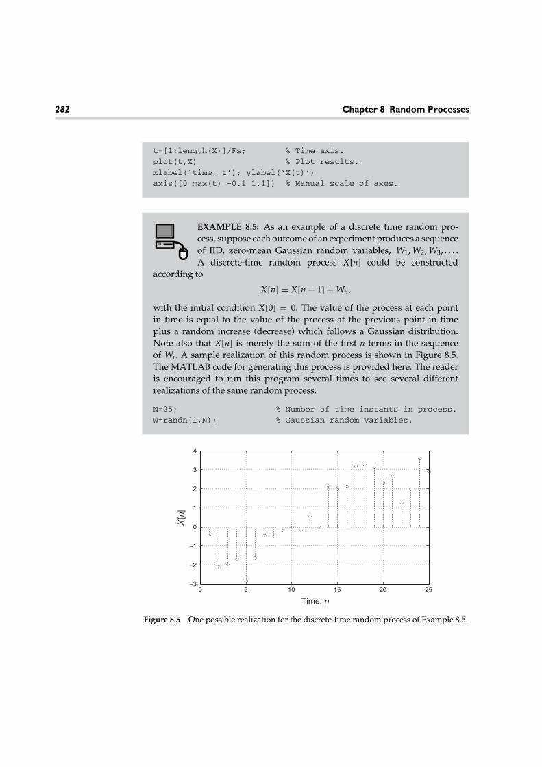
282 Chapter 8 Random Processes
t=[1:length(X)]/Fs; % Time axis.
plot(t,X) % Plot results.
xlabel(‘time, t’); ylabel(‘X(t)’)
axis([0 max(t) -0.1 1.1]) % Manual scale of axes.
EXAMPLE 8.5: As an example of a discrete time random pro-cess, suppose each outcome of an experiment produces a sequenceof IID, zero-mean Gaussian random variables, W1, W2, W3, . . . .A discrete-time random process X[n] could be constructed
according to
X[n] = X[n − 1] + Wn,
with the initial condition X[0] = 0. The value of the process at each pointin time is equal to the value of the process at the previous point in timeplus a random increase (decrease) which follows a Gaussian distribution.Note also that X[n] is merely the sum of the first n terms in the sequenceof Wi. A sample realization of this random process is shown in Figure 8.5.The MATLAB code for generating this process is provided here. The readeris encouraged to run this program several times to see several differentrealizations of the same random process.
N=25; % Number of time instants in process.
W=randn(1,N); % Gaussian random variables.
0 5 10 15 20 25−3
−2
−1
0
1
2
3
4
Time, n
X[n
]
Figure 8.5 One possible realization for the discrete-time random process of Example 8.5.

8.2 Mathematical Tools for Studying Random Processes 283
X=[0 cumsum(W)]; % Samples of X[n].
stem([0:N],X,‘o’) % Plot realization of X[n].
xlabel(‘time, n’); ylabel(‘X[n]’);
8.2 Mathematical Tools for StudyingRandom Processes
As with random variables, we can mathematically describe a random process interms of a cumulative distribution function, a probability density function, or aprobability mass function. In fact, given a random process, X(t), which is sampledat some specified point in time, t = tk, the result is a random variable, Xk = X(tk).This random variable can then be described in terms of its PDF, fX(xk; tk). Note thatan additional time variable has been added to the PDF. This is necessary due to thefact that the PDF of the sample of the random process may depend on when theprocess is sampled. If desired, the CDF or PMF can be used rather than the PDF todescribe the sample of the random process.
EXAMPLE 8.6: Consider the random telegraph signal of Example 8.4.Since this process is binary-valued, any sample will be a Bernoullirandom variable. The only question is, What is the probability thatXk = X(tk) is equal to 1 (or 0)? Suppose that there are exactly n switchesin the time interval [0, tk). Then X(tk) = n mod 2. Stated another way,define Sn = T1 + T2 + · · · + Tn. There will be exactly n switches in thetime interval [0, tk) provided that Sn < tk < Sn+1. Hence,
Pr(n switches in [0, tk)) = Pr(Sn < tk < Sn+1)
=∫
Pr(Sn < tk < Sn+1|Sn = s)fSn (s) ds
=∫ tk
0Pr(tk < Sn+1|Sn = s)fSn (s) ds =
∫ tk
0Pr(Tn+1 > tk − s)fSn (s) ds.
Since the Ti are IID and exponential, Sn will follow a Gammadistribution. Using the Gamma PDF for fSn (s) and the fact that

284 Chapter 8 Random Processes
0 0.5 1 1.5 2 2.5 30
0.1
0.2
0.3
0.4
0.5
0.6
0.7
0.8
0.9
1
Time, t
Pro
babi
lity
Pr(X(t )=1)
Pr(X(t )=0)
Figure 8.6 Time dependence of the PMF for the random telegraph signal.
Pr(Tn+1 > tk − s) = exp (−λ(tk − s)) results in
Pr(n switches in [0, tk)) =∫ tk
0e−λ(tk−s) λnsn−1
(n − 1)! e−λs ds
= λne−λtk
(n − 1)!∫ tK
0sn−1 ds = (λtk)n
n! e−λtk .
So, it is seen that the number of switches in the interval [0, tk) followsa Poisson distribution. The sample of the random process will be equalto 0 if the number of switches is even. Hence,
Pr(X(tk) = 0) =∑
n even
Pr(n switches in [0, tk))
=∑
n even
(λtk)n
n! e−λtk = e−λtk cosh(λtk) = 12 + 1
2 e−2λtk .
Likewise,
Pr(X(tk) = 1) =∑
n odd
Pr(n switches in [0, tk))
=∑
n odd
(λtk)n
n! e−λtk = e−λtk sinh(λtk) = 12 − 1
2 e−2λtk .
The behavior of this distribution as it depends on time should makeintuitive sense. For very small values of tk, it is most likely that there
8.2 Mathematical Tools for Studying Random Processes 285
are no switches in the interval [0, tk), in which case Pr(X(tk) = 0) shouldbe close to 1. On the other hand, for large tk, many switches will likelyoccur and it should be almost equally likely that the process will takeon the values of 0 or 1.
EXAMPLE 8.7: Now consider the PDF of a sample of the discrete-timeprocess of Example 8.5. Note that since X[n] is formed by summing nIID Gaussian random variables, X[n] will itself be a Gaussian randomvariable with mean of E[X[n]] = nµW and variance Var(X[n]) = nσ 2
W .In this case, since the Wi were taken to be zero mean, the PDF of X[n] is
fX(x; n) = 1√2πnσ 2
W
exp
(− x2
2nσ 2W
).
Once again, we see that for this example, the form of the PDF doesindeed depend on when the sample is taken.
The PDF (or CDF or PMF) of a sample of a random process taken at an arbitrarypoint in time goes a long way toward describing the random process, but it isnot a complete description. To see this, consider two samples, X1 = X(t1) andX2 = X(t2), taken at two arbitrary points in time. The PDF, fX(x; t), describes bothX1 and X2, but it does not describe the relationship between X1 and X2. For somerandom processes, it might be reasonable to expect that X1 and X2 would be highlycorrelated if t1 is near t2, while X1 and X2 might be virtually uncorrelated if t1 andt2 are far apart. To characterize relationships of this sort, a joint PDF of the twosamples would be needed. Hence, it would be necessary to construct a joint PDF ofthe form fX1,X2 (x1, x2; t1, t2). This is referred to as a second order PDF of the randomprocess X(t).
Continuing with this reasoning, in order to completely describe the randomprocess, it is necessary to specify an nth order PDF for an arbitrary n. That is, sup-pose random process is sampled at time instants t1, t2, . . . , tn, producing the randomvariables X1 = X(t1), X2 = X(t2), . . . , Xn = X(tn). The joint PDF of the n samples,fX1,X2,...,Xn (x1, x2, . . . , xn; t1, t2, . . . , tn), for an arbitrary n and arbitrary sampling timeswill give a complete description of the random process. In order to make this nota-tion more compact, the vectors X = (X1, X2, . . . , Xn)T , x = (x1, x2, . . . , xn)T , andt = (t1, t2, . . . , tn)T are introduced and the nth order joint PDF is written as fX(x;t).
Unfortunately, for many realistic random processes, the prospects of writingdown an nth order PDF is rather daunting. One notable exception is the Gaussian

286 Chapter 8 Random Processes
random process, which will be described in detail in Section 8.5. However, formost other cases, specifying a joint PDF of n samples may be exceedingly difficult,and hence it is necessary to resort to a simpler but less complete description of therandom process. The simplest is the mean function of the process.
DEFINITION 8.2: The mean function of a random process is simply the expectedvalue of the process. For continuous time processes this is written as
µX(t) = E[X(t)] =∫ ∞
−∞xfX(x; t) dx, (8.1)
while for discrete time processes, the following notation is used:
µX[n] = E[X[n]] =∫ ∞
−∞xfX(x; n) dx. (8.2)
In general, the mean of a random process may change with time, but in many cases,this function is constant. Also, it is noted that only the first order PDF of the processis needed to compute the mean function.
EXAMPLE 8.8: Consider the random telegraph process of Example 8.4.It was shown in Example 8.6 that the first order PMF of this process wasdescribed by a Bernoulli distribution with
Pr(X(t) = 1) = 12 − 1
2 exp(−λt).
The mean function then follows as
µX(t) = E[X(t)] = 1∗ Pr(X(t) = 1) + 0∗ Pr(X(t) = 0) = 12 − 1
2 exp(−λt).
EXAMPLE 8.9: Next, consider the sinusoidal random process ofExample 8.2 where X(t) = A sin(ωot) and A was a uniform randomvariable over [0, 1). In this case,
µX(t) = E[X(t)] = E[A sin(ωot)] = E[A] sin(ωot) = 12 sin(ωot).
This example illustrates a very important concept in that quite often itis not necessary to explicitly evaluate the first order PDF of a randomprocess in order to evaluate its mean function.
8.2 Mathematical Tools for Studying Random Processes 287
EXAMPLE 8.10: Now suppose the random process of the previousexample is slightly modified. In particular, consider a sine-wave pro-cess where the random variable is the phase, �, which is uniformlydistributed over [0, 2π ). That is, X(t) = a sin(ωot +�). For this example,the amplitude of the sine wave, a, is taken to be fixed (not random). Themean function is then
µX(t) = E[X(t)] = E[a sin(ωot + �)] = a∫
f�(θ ) sin(ωot + θ ) dθ
= a2π
∫ 2π
0sin(ωot + θ ) dθ = 0,
which is a constant. Why is the mean function of the previous examplea function of time and this one is not? Consider the member functionsof the respective ensembles for the two random processes.
EXAMPLE 8.11: Now consider a sinusoid with a random fre-quency X(t) = cos(2πFt), where F is a random variable uniformlydistributed over some interval (0, fo). The mean function can bereadily determined to be
µX(t) = E[cos(2πFt)] = 1fo
∫ fo
0cos(2π ft) df = sin(2π fot)
2π fot= sinc (2fot).
We can also estimate the mean function through simulation. We provide someMATLAB code to produce many realizations of this random process. Themean function is then found by taking the sample mean of all the realizationscreated. The sample mean and the ensemble mean are shown in Figure 8.7.Naturally, more or less accuracy in the sample mean can be obtained byvarying the number of realizations generated.
fo=2; % Maximum frequency.
N=1000; % Number of realizations.
t=[-4.995:0.01:4.995]; % Time axis.
F=fo*rand(N,1); % Uniform frequencies.
x=cos(2*pi*F*t); % Each row is a
% realization of process.
sample_mean=sum(x)/N; % Compute sample mean.

288 Chapter 8 Random Processes
−5 −4 −3 −2 −1 0 1 2 3 4 5−0.4
−0.2
0
0.2
0.4
0.6
0.8
1
t (seconds)
µ(t)
Figure 8.7 Comparison of the sample mean and ensemble mean for the sinusoid withrandom frequency of Example 8.11. The solid line is the sample mean, while the dashed lineis the ensemble mean.
true_mean=sin(2*pi*fo*t)./(2*pi*fo*t); % Compute ensemble
mean.
plot(t,sample_mean,‘-’,t,true_mean,‘--’) % Plot results.
xlabel(‘t (seconds)’); ylabel(‘mu(t)’);
To partially describe the second order characteristics of a random process, theautocorrelation function is introduced.
DEFINITION 8.3: The autocorrelation function, RXX(t1, t2), of a continuous timerandom process, X(t), is defined as the expected value of the product X(t1)X(t2):
RXX(t1, t2) = E[X(t1)X(t2)] =∞∫∫
−∞x1x2fX1,X2 (x1, x2; t1, t2) dx1 dx2. (8.3)
For discrete time processes, the autocorrelation function is
RXX[n1, n2] = E[X[n1]X[n2]] =∞∫∫
−∞x1x2fX1,X2 (x1, x2; n1, n2) dx1 dx2. (8.4)
Naturally, the autocorrelation function describes the relationship (correlation)between two samples of a random process. This correlation will depend on when

8.2 Mathematical Tools for Studying Random Processes 289
the samples are taken; thus, the autocorrelation function is, in general, a functionof two time variables. Quite often we are interested in how the correlation betweentwo samples depends on how far apart the samples are spaced. To explicitlydraw out this relationship, define a time difference variable, τ = t2 − t1, andthe autocorrelation function can then be expressed as
RXX(t, t + τ ) = E[X(t)X(t + τ )], (8.5)
where we have replaced t1 with t to simplify the notation even further.
EXAMPLE 8.12: Consider the sine wave process with a uniformly dis-tributed amplitude as described in Examples 8.2 and 8.9, where X(t) =A sin(ωot). The autocorrelation function is found as
RXX(t1, t2) = E[X(t1)X(t2)] = E[A2 sin(ωot1) sin(ωot2)]= 1
3 sin(ωot1) sin(ωot2),
or
RXX(t, t + τ ) = 13 sin(ωot) sin(ωo(t + τ )).
EXAMPLE 8.13: Now consider the sine wave process with randomphase of Example 8.10 where X(t) = a sin(ωot + �). Then
RXX(t1, t2) = E[X(t1)X(t2)] = E[a2 sin(ωot1 + θ ) sin(ωot2 + θ )].To aid in calculating this expected value, we use the trigonometricidentity
sin(x) sin(y) = 12 cos(x − y) − 1
2 cos(x + y).
The autocorrelation then simplifies to
RXX(t1, t2) = a2
2E[cos(ωo(t2 − t1))] + a2
2E[cos(ωo(t1 + t2 + 2θ ))]
= a2
2cos(ωo(t2 − t1)),
or
RXX(t, t + τ ) = a2
2cos(ωoτ ).

290 Chapter 8 Random Processes
Note that in this case, the autocorrelation function is only a functionof the difference between the two sampling times. That is, it does notmatter where the samples are taken, only how far apart they are.
EXAMPLE 8.14: Recall the random process of Example 8.5, whereX[n] = X[n − 1] + Wn, X[0] = 0 and the Wn were a sequence of IID zeromean Gaussian random variables. In this case, it is easier to calculatethe autocorrelation function using the alternative expression,
X[n] =n∑
i=1
Wi.
Then
RXX[n1, n2] = E[X[n1]X[n2]] = E
n1∑
i=1
Wi
n2∑j=1
Wj
=
n1∑i=1
n2∑j=1
E[WiWj].
Since the Wi are IID and zero-mean, E[WiWj] = 0 unless i = j. Hence,
RXX[n1, n2] = min(n1, n2)σ 2W .
DEFINITION 8.4: The autocovariance function, CXX(t1, t2), of a continuous timerandom process, X(t), is defined as the covariance of X(t1) and X(t2):
CXX(t1, t2) = Cov(X(t1), X(t2)) = E[(X(t1) − µX(t1))(X(t2) − µX(t2))]. (8.6)
The definition is easily extended to discrete time random processes.
As with the covariance function for random variables, the autocovariancefunction can be written in terms of the autocorrelation function and the meanfunction:
CXX(t1, t2) = RXX(t1, t2) − µX(t1)µX(t2). (8.7)
Once the mean and autocorrelation functions of a random process have beencomputed, the autocovariance function is trivial to find.
The autocovariance function is helpful when studying random processes thatcan be represented as the sum of a deterministic signal, s(t), plus a zero-mean noise

8.3 Stationary and Ergodic Random Processes 291
process, N(t). If X(t) = s(t) + N(t), then the autocorrelation function of X(t) is
RXX(t1, t2) = E[(s(t1) + N(t1))(s(t2) + N(t2))] = s(t1)s(t2) + RNN(t1, t2), (8.8)
using the fact that µN(t) = 0. If the signal is strong compared to the noise, thedeterministic part will dominate the autocorrelation function, and hence RXX(t1, t2)will not tell us much about the randomness in the process X(t). On the other hand,the autocovariance function is
CXX(t1, t2) = RXX(t1, t2) − s(t1)s(t2) = RNN(t1, t2) = CNN(t1, t2). (8.9)
Hence, the autocovariance function allows us to isolate the noise that is the sourceof randomness in the process.
DEFINITION 8.5: For a pair of random processes X(t) and Y(t), the crosscorrela-tion function is defined as
RXY(t1, t2) = E[X(t1)Y(t2)]. (8.10)
Likewise, the cross-covariance function is
CXY(t1, t2) = E[(X(t1) − µX(t1))(Y(t2) − µY(t2))]. (8.11)
EXAMPLE 8.15: Suppose X(t) is a zero-mean random process withautocorrelation function RXX(t1, t2). A new process Y(t) is formed bydelaying X(t) by some amount td. That is, Y(t) = X(t − td). Then thecrosscorrelation function is
RXY(t1, t2) = E[X(t1)Y(t2)] = E[X(t1)X(t2 − td)] = RXX(t1, t2 − td).
In a similar fashion, it is seen that RYX(t1, t2) = RXX(t1 − td, t2) andRYY(t1, t2) = RXX(t1 − td, t2 − td).
8.3 Stationary and Ergodic RandomProcesses
From the few simple examples given in the preceding section, we conclude that themean function and the autocorrelation (or autocovariance) function can provide

292 Chapter 8 Random Processes
information about the temporal structure of a random process. We will delve intothe properties of the autocorrelation function in more detail later in the chapter,but first the concepts of stationarity and ergodicity must be introduced.
DEFINITION 8.6: A continuous time random process X(t) is strict sense stationaryif the statistics of the process are invariant to a time shift. Specifically, for any timeshift τ and any integer n ≥ 1,
fX1,X2,...,Xn (x1, x2, . . . , xn; t1, t2, . . . , tn)
= fX1,X2,...,Xn (x1, x2, . . . , xn; t1 + τ , t2 + τ , . . . , tn + τ ). (8.12)
In general, it is quite difficult to show that a random process is strict sensestationary since to do so, one needs to be able to express the general nth order PDF.On the other hand, to show that a process is not strict sense stationary, one needs toshow only that one PDF of any order is not invariant to a time shift. One exampleof a process that can be shown to be stationary in the strict sense is an IID process.That is, suppose X(t) is a random process that has the property that X(t) has anidentical distribution for any t and that X(t1) and X(t2) are independent for anyt1 �= t2. In this case,
fX1,X2,...,Xn (x1, x2, . . . , xn; t1, t2, . . . , tn) =n∏
i=1
fXi (xi; ti). (8.13)
Since the nth order PDF is the product of first order PDFs and the first order PDFis invariant to a time shift, then the nth order PDF must be invariant to a time shift.
EXAMPLE 8.16: Consider the sinusoidal process with random ampli-tude from Example 8.2, where X(t) = A sin(ωot). This process isclearly not stationary since if we take any realization of the process,x(t) = a sin(ωot), then a time shift x(t + τ ) = a sin(ωo(t + τ )) would notbe a realization in the original ensemble. Now suppose the process hasa random phase rather than a random amplitude as in Example 8.10,resulting in X(t) = a sin(ωot + �). It was already shown in Example8.10 that µX(t) = 0 for this process, and hence the mean function isinvariant to a time shift. Furthermore, in Example 8.13 it was shownthat RXX(t, t + τ ) = (a2/2) cos(ωoτ ), and hence the autocorrelation func-tion is also invariant to a time shift. It is not difficult to show that thefirst order PDF follows an arcsine distribution:
fX(x; t) = 1
π√
1 − x2, −1 < x < 1,

8.3 Stationary and Ergodic Random Processes 293
and it is also independent of time and thus invariant to a time shift.It seems that this process might be stationary in the strict sense, but itwould be rather cumbersome to prove it because the nth order PDF isdifficult to specify.
As was seen in Example 8.16, it may be possible in some examples to determinethat some of the statistics of a random process are invariant to time shifts, butdetermining stationarity in the strict sense may be too big of a burden. In thosecases, we often settle for a looser form of stationarity.
DEFINITION 8.7: A random process is wide sense stationary (WSS) if the meanfunction and autocorrelation function are invariant to a time shift. In particular,this implies that
µX(t) = µX = constant, (8.14)
RXX(t, t + τ ) = RXX(τ ) (function only of τ ). (8.15)
All strict sense stationary random processes are also WSS, provided that the meanand autocorrelation function exist. The converse is not true. A WSS process doesnot necessarily need to be stationary in the strict sense. We refer to a process thatis not WSS as nonstationary.
EXAMPLE 8.17: Suppose we form a random process Y(t) by modu-lating a carrier with another random process, X(t). That is, let Y(t) =X(t) cos(ωot+�) where � is uniformly distributed over [0, 2π ) and inde-pendent of X(t). Under what conditions is Y(t) WSS? To answer this,we calculate the mean and autocorrelation function of Y(t).
µY(t) = E[X(t) cos(ωot + �)] = E[X(t)]E[cos(ωot + �)] = 0;
RYY(t,t+τ )=E[X(t)X(t+τ )cos(ωot)cos(ωo(t+τ ))]=E[X(t)X(t+τ )]
{12 cos(ωoτ )+ 1
2 E[cos(ωo(2t+τ )+2�)]}
= 12 RXX(t,t+τ )cos(ωoτ )
While the mean function is a constant, the autocorrelation is not neces-sarily only a function of τ . The process Y(t) will be WSS provided thatRXX(t, t +τ ) = RXX(τ ). Certainly if X(t) is WSS, then Y(t) will be as well.

294 Chapter 8 Random Processes
EXAMPLE 8.18: Let X(t) = At + B where A and B are independentrandom variables, both uniformly distributed over the interval (−1, 1).To determine whether this process is WSS, calculate the mean andautocorrelation functions:
µX(t) = E[At + B] = E[A]t + E[B] = 0;
RXX(t, t + τ ) = E[(At + B)(A(t + τ ) + B)]= E[A2]t(t + τ ) + E[B2] + E[AB](2t + τ ) = 1
3 t(t + τ ) + 13 .
Clearly, this process is not WSS.
Many of the processes we deal with are WSS and hence have a constant meanfunction and an autocorrelation function that depends only on a single time vari-able. Hence, in the remainder of the text, when a process is known to be WSS or ifwe are assuming it to be WSS, then we will represent its autocorrelation functionby RXX(τ ). If a process is nonstationary or if we do not know if the process is WSS,then we will explicitly write the autocorrelation function as a function of two vari-ables, RXX(t, t + τ ). For example, if we say that a process has a mean function ofµX = 1 and an autocorrelation function, RXX(τ ) = exp(−|τ |), then the reader caninfer that the process is WSS, even if it is not explicitly stated.
In order to calculate the mean or autocorrelation function of a random process,it is necessary to perform an ensemble average. In many cases, this may not bepossible as we may not be able to observe all realizations (or a large number ofrealizations) of a random process. In fact, quite often we may be able to observeonly a single realization. This would occur in situations where the conditions ofan experiment cannot be duplicated and hence the experiment is not repeatable.Is it possible to calculate the mean and/or autocorrelation function from a singlerealization of a random process? The answer is, sometimes, depending on thenature of the process.
To start with, consider the mean. Suppose a WSS random process X(t) has amean µX . We are able to observe one realization of the random process, x(t), andwish to try to determine µX from this realization. One obvious approach would beto calculate the time average1 of the realization:
〈x(t)〉 = limto→∞
12to
∫ to
−to
x(t) dt. (8.16)
1Throughout the text, angular brackets 〈 〉 are used as a shorthand notation to representthe time average operator.

8.3 Stationary and Ergodic Random Processes 295
However, it is not obvious if the time average of one realization is necessarily equalto the ensemble average. If the two averages are the same, then we say that therandom process is ergodic in the mean.
One could take the same approach for the autocorrelation function. Given asingle realization, x(t), form the time-average autocorrelation function:
xx(τ ) = 〈x(t)x(t + τ )〉 = limto→∞
12to
∫ to
−to
x(t)x(t + τ ) dt. (8.17)
If xx(τ ) = RXX(τ ) for any realization, x(t), then the random process is said tobe ergodic in the autocorrelation. In summary, we have the following definition ofergodicity:
DEFINITION 8.8: A WSS random process is ergodic if ensemble averages involv-ing the process can be calculated using time averages of any realization of theprocess. Two limited forms of ergodicity are
(1) ergodic in the mean: 〈x(t)〉 = E[X(t)];(2) ergodic in the autocorrelation: 〈x(t + τ )〉 = E[X(t)X(t + τ )].
EXAMPLE 8.19: As a simple example, suppose X(t) = A, where A is arandom variable with some arbitrary PDF fA(a). Note that this processis stationary in the strict sense since for any realization, x(t) = x(t + τ ).That is, not only are the statistics of the process invariant to time shifts,but every realization is also invariant to any time shift. If we take thetime average of a single realization, x(t) = a, we get 〈x(t)〉 = a. Hence,each different realization will lead to a different time average and willnot necessarily give the ensemble mean, µA. Although this process isstationary in the strict sense, it is not ergodic in any sense.
EXAMPLE 8.20: Now consider the sinusoid with random phase X(t) =a sin(ωot + �), where � is uniform over [0, 2π ). It was demonstratedin Example 8.13 that this process is WSS. But is it ergodic? Given anyrealization x(t) = a sin(ωot + θ ), the time average is 〈x(t)〉 = 〈a sin(ωot +θ )〉 = 0. That is, the average value of any sinusoid is zero. So this processis ergodic in the mean since the ensemble average of this process wasalso zero. Next, consider the sample autocorrelation function:
〈x(t)x(t + τ )〉 = a2〈sin(ωot + θ ) sin(ωot + ωoτ + θ )〉
= a2
2〈cos(ωoτ )〉 − a2
2〈cos(2ωot + ωoτ + 2θ )〉 = a2
2cos(ωoτ ).

296 Chapter 8 Random Processes
This also is exactly the same expression obtained for the ensemble aver-aged autocorrelation function. Hence, this process is also ergodic in theautocorrelation.
EXAMPLE 8.21: For a process that is known to be ergodic, theautocorrelation function can be estimated by taking a sufficientlylong time average of the autocorrelation function of a single real-ization. We demonstrate this via MATLAB for a process that
consists of a sum of sinusoids of fixed frequencies and random phases,
X(t) =n∑
k=1
cos(2π fkt + θk),
where the θk are IID and uniform over (0, 2π ). For an arbitrary signal x(t), wenote the similarity between the time averaged autocorrelation function andthe convolution of x(t) and x(−t). If we are given a single realization, x(t),which lasts only for the time interval, (−to, to), then these two expressions aregiven by
〈x(t)x(t + τ )〉 = 12to − τ
∫ to−τ
−to
x(t)x(t + τ ) dt,
x(t) ∗ x(−t) =∫ to−τ
−to
x(t)x(t + τ ) dt,
for τ > 0. In general, we have the relationship
〈x(t)x(t + τ )〉 = x(t) ∗ x(−t)2to − |τ | .
By using the MATLAB convolution function, conv, the time averaged auto-correlation can easily be computed. This is demonstrated in the code thatfollows. Figure 8.8 shows a comparison between the ensemble averagedautocorrelation and the time averaged autocorrelation taken from a singlerealization. From the figure, it is noted that the agreement between the twois good for τ � to but not good when τ ∼ to. This is due to the fact that whenτ approaches to, the time window over which the time average is computedgets too small to produce an accurate estimate.
N=4; % Number of sinusoids.
to=5; % Time duration.

8.3 Stationary and Ergodic Random Processes 297
−10 −8 −6 −4 −2 0 2 4 6 8 10
−2
−1.5
−1
−0.5
0
0.5
1
1.5
2
τ
Rxx
(τ)
Figure 8.8 Comparison of the time-average autocorrelation and the ensemble-averageautocorrelation for the sum of sinusoids process of Example 8.21. The solid line is the time-average autocorrelation, while the dashed line is the ensemble-average autocorrelation.
Ts=0.01; % Sample interval.
t=[-to:Ts:to]; % Time axis.
tau=[-2*to:Ts:2*to]; % Tau axis.
theta=rand(1,N); % Random phases.
f=1./[1:N]; % Frequencies (not
random).
x=zeros(size(t));
True_Rxx=zeros(size(tau));
for k=1:N
x=x+cos(2*pi*f(k)*t+2*pi*theta(k)); % Construct process.
True_Rxx=True_Rxx+cos(2*pi*f(k)*tau)/2; % Compute Rxx(tau).
end
z=conv(x,fliplr(x)); % x(t)*x(-t)
Rxx=Ts*z./(2*to-abs(tau)); % Time averaged Rxx.
plot(tau,Rxx,‘-’,tau,True_Rxx,‘--’) % Plot results.
xlabel(‘tau’); ylabel(‘R_X_X(tau)’)
axis([-2*to 2*to -1.1*N/2 1.1*N/2])
The previous examples show two different random processes, one that isergodic and one that is not. What characteristics of a random process make it

298 Chapter 8 Random Processes
ergodic? To get some better insight toward answering this question, consider adiscrete time process, X[n], where each random variable in the sequence is IID andconsider forming the time average:
〈X[n]〉 = limm→∞
1m
m∑n=1
X[n]. (8.18)
The right-hand side of this equation is nothing more than the sample mean. Byvirtue of the law of large numbers, the limit will indeed converge to the ensemblemean of the random process, µX , and hence this process is ergodic in the mean. Inthis case, the time average converges to the ensemble average because each timesample of the random process gives an independent observation of the underlyingrandomness. If the samples were highly correlated, then taking more sampleswould not necessarily cause the sample mean to converge to the ensemble mean.So, it seems that the form of the autocorrelation function will play some role indetermining if a random process is ergodic in the mean.
To formalize this concept, consider the time average of an arbitrary WSS randomprocess:
〈X(n)〉 = limto→∞ Xto where Xto = 1
2to
∫ to
−to
X(t) dt. (8.19)
Note that Xto is a random variable with an expected value given by2
E[Xto ] = E[
12to
∫ to
−to
X(t) dt]
= 12to
∫ to
−to
E[X(t)] dt = 12to
∫ to
−to
µX dt = µX . (8.20)
Hence, Xto is an unbiased estimate of the true mean, but for the process to be ergodicin the mean, it is required that Xto converge to µX as to → ∞. This convergencewill occur (in the mean square sense) if the variance of Xto goes to zero in the limitas to → ∞. To see under what conditions this occurs, we calculate the variance.
Var(Xto )=E[(Xto −µX)2]=E
[(1
2to
∫ to
−to
(X(t)−µX)dt)2]
= 14t2
o
∫ to
−to
∫ to
−to
E[(X(t)−µX)(X(s)−µX)]dt ds= 14t2
o
∫ to
−to
∫ to
−to
CXX(t,s)dt ds.
(8.21)
2We exchange the order of expectation and integration since they are both linearoperators.

8.3 Stationary and Ergodic Random Processes 299
Since the random process X(t) is WSS, the autocovariance is only a function ofτ = t − s. As a result, the double integral can be converted to a single integral.3 Theresult is
Var(Xto ) = 12to
∫ 2to
−2to
(1 − |τ |
2to
)CXX(τ ) dτ = 1
to
∫ 2to
0
(1 − τ
2to
)CXX(τ ) dτ . (8.22)
Thus, the random process will be ergodic in the mean if this expression goes tozero in the limit as to → ∞. This proves the following theorem.
THEOREM 8.1: A continuous WSS random process X(t) will be ergodic in themean if
limto→∞
1to
∫ 2to
0
(1 − τ
2to
)CXX(τ ) dτ = 0. (8.23)
One implication of Theorem 8.1 is that if CXX(τ ) tends toward a constant asτ → ∞, then that constant must be zero for the process to be ergodic. Stated interms of the autocorrelation function, a sufficient condition for a process to beergodic in the mean is that
limτ→∞ RXX(τ ) = µ2
X . (8.24)
Similar relationships can be developed to determine when a process is ergodic inthe autocorrelation, but that topic is beyond the intended scope of this text.
EXAMPLE 8.22: Consider the process X(t) = A of Example 8.19. It iseasily found that the autocovariance function of this process is CXX(τ ) =σ 2
A for all τ . Plugging this into the left-hand side of Equation 8.23results in
limto→∞
1to
∫ 2to
0
(1 − τ
2to
)CXX(τ ) dτ = lim
to→∞σ 2
Ato
∫ 2to
0
(1 − τ
2to
)dτ
= limto→∞
σ 2A
toto = σ 2
A.
Since this limit is not equal to zero, the process clearly does not meetthe condition for ergodicity. Next, consider the sinusoidal process of
3The procedure for doing this conversion will be described in detail in Chapter 10,where a similar integral will be encountered in the proof of the Wiener–Khintchine–Einsteintheorem.

300 Chapter 8 Random Processes
Example 8.20. In that case, the autocovariance function is CXX(τ ) =(a2/2) cos(ωoτ ) and the left-hand side of Equation 8.23 produces
limto→∞
1to
∫ 2to
0
(1 − τ
2to
)CXX(τ ) dτ = lim
to→∞a2
2to
∫ 2to
0
(1 − τ
2to
)cos(ωoτ ) dτ
= limto→∞ a2
(1 − cos(2ωoto)
(2ωoto)2
)= 0.
So, even though this autocorrelation function does not approach zero inthe limit at τ → 0 (it oscillates), it still meets the condition for ergodicity.
8.4 Properties of the AutocorrelationFunction
Since the autocorrelation function, along with the mean, is considered to be aprincipal statistical descriptor of a WSS random process, we will now considersome properties of the autocorrelation function. It should quickly become apparentthat not just any function of τ can be a valid autocorrelation function.
PROPERTY 8.4.1: The autocorrelation function evaluated at τ = 0, RXX(0), is theaverage normalized power in the random process, X(t).
To clarify this, note that RXX(0) = E[X2(t)]. Now suppose the random processX(t) was a voltage measured at some point in a system. For a particular realization,x(t), the instantaneous power would be p(t) = x2(t)/r, where r is the impedancein Ohms (�). The average power (averaged over all realizations in the ensemble)would then be Pavg = E[X2(t)]/r = RXX(0)/r. If, on the other hand, X(t) were acurrent rather than a voltage, then the average power would be Pavg = RXX(0)r.From a systems level, it is often desirable not to concern ourselves with whether asignal is a voltage or a current. Accordingly, it is common to speak of a normalizedpower, which is the power measured using a 1-� impedance. With r = 1, thetwo expressions for average power are the same and equal to the autocorrelationfunction evaluated at zero.
PROPERTY 8.4.2: The autocorrelation function of a WSS random process is aneven function; that is, RXX(τ ) = RXX(−τ ).

8.5 Gaussian Random Processes 301
This property can easily be established from the definition of autocorrelation.Note that RXX(−τ ) = E[X(t)X(t −τ )]. Since X(t) is WSS, this expression is the samefor any value of t. In particular, replace t in the previous expression with t + τ sothat RXX(−τ ) = E[X(t+τ )X(t)] = RXX(τ ). As a result of this property, any functionof τ which is not even cannot be a valid autocorrelation function.
PROPERTY 8.4.3: The autocorrelation function of a WSS random process ismaximum at the origin; that is, |RXX(τ )| ≤ RXX(0) for all τ .
This property is established using the fact that for any two random variables,X and Y,
(E[XY])2 ≤ E[X2]E[Y2]. (8.25)
This fact was previously demonstrated in the proof of Theorem 5.4. LettingX = X(t) and Y = X(t + τ ) results in
R2XX(τ ) = {E[X(t)X(t + τ )]}2 ≤ E[X2(t)]E[X2(t + τ )] = R2
XX(0). (8.26)
Taking square roots of both sides results in Property 8.4.3.
PROPERTY 8.4.4: If X(t) is ergodic and has no periodic components, thenlimτ→∞ RXX(τ ) = µ2
X .
PROPERTY 8.4.5: If X(t) has a periodic component, then RXX(t) will have aperiodic component with the same period.
From these properties it is seen that an autocorrelation function can oscillate,can decay slowly or rapidly, and can have a nonzero constant component. Asthe name implies, the auto-correlation function is intended to measure the extentof correlation of samples of a random process as a function of how far apart thesamples are taken.
8.5 Gaussian Random Processes
One of the most important classes of random processes is the Gaussian randomprocess, which is defined as follows.
DEFINITION 8.9: A random process, X(t), for which any n samples, X1 =X(t1), X2 = X(t2), . . . , Xn = X(tn), taken at arbitrary points in time t1, t2, . . . , tn,

302 Chapter 8 Random Processes
form a set of jointly Gaussian random variables for any n = 1, 2, 3, . . . is a Gaussianrandom process.
In vector notation, the vector of n samples, X = [X1, X2, . . . , Xn]T , will have a jointPDF given by
fX(x) = 1√(2π )n det(CXX)
exp(− 1
2 (x − µX)TC−1XX(x − µX)
). (8.27)
As with any joint Gaussian PDF, all that is needed to specify the PDF is the meanvector and the covariance matrix. When the vector of random variables consistsof samples of a random process, to specify the mean vector, all that is neededis the mean function of the random process, µX(t), since that will give the meanfor any sample time. Similarly, all that is needed to specify the elements of thecovariance matrix, Ci,j = Cov(X(ti), X(tj)), would be the autocovariance functionof the random process, CXX(t1, t2) or, equivalently, the autocorrelation function,RXX(t1, t2), together with the mean function. Hence, the mean and autocorrelationfunctions provide sufficient information to specify the joint PDF for any numberof samples of a Gaussian random process. Note that since any nth order PDF iscompletely specified by µX(t) and RXX(t1, t2), if a Gaussian random process is WSS,then the mean and autocorrelation functions will be invariant to a time shift andhence any PDF will be invariant to a time shift. Therefore, any WSS Gaussianrandom process is also stationary in the strict sense.
EXAMPLE 8.23: Consider the random process X(t) = A cos(ωot) +B sin(ωot), where A and B are independent, zero-mean Gaussian randomvariables with equal variances of σ 2. This random process is formed as alinear combination of two Gaussian random variables, and hence sam-ples of this process are also Gaussian random variables. The mean andautocorrelation functions of this process are found as
µX(t) = E[A cos(ωot) + B sin(ωot)] = E[A] cos(ωot) + E[B] sin(ωot) = 0,
RXXa(t1, t2) = E[(A cos(ωot1) + B sin(ωot1))(A cos(ωot2) + B sin(ωot2))]= E[A2] cos(ωot1) cos(ωot2) + E[B2] sin(ωot1) sin(ωot2)
+ E[AB]{cos(ωot1) sin(ωot2) + sin(ωot1) cos(ωot2)}= σ 2{cos(ωot1) cos(ωot2) + sin(ωot1) sin(ωot2)}= σ 2 cos(ωo(t2 − t1)).
Note that this process is WSS since the mean is constant and the autocor-relation function depends only on the time difference. Since the process

8.6 Poisson Processes 303
is zero-mean, the first order PDF is that of a zero-mean Gaussian randomvariable:
fX(x; t) = 1√2πσ 2
exp
(− x2
2σ 2
).
This PDF is independent of time as would be expected for a stationaryrandom process. Now consider the joint PDF of two samples, X1 = X(t)and X2 = X(t + τ ). Since the process is zero-mean, the mean vector issimply the all-zeros vector. The covariance matrix is then of the form
CXX =[
RXX(0) RXX(τ )RXX(τ ) RXX(0)
]= σ 2
[1 cos(ωoτ )
cos(ωoτ ) 1
].
The joint PDF of the two samples would then be
fX1,X2 (x1,x2;t,t+τ )= 12πσ 2|sin(ωoτ )| exp
(−x2
1 −2x1x2 cos(ωoτ )+x22
2σ 2 sin2(ωoτ )
).
Note once again that this joint PDF is dependent only on time difference,τ , and not on absolute time t. Higher order joint PDFs could be workedout in a similar manner.
8.6 Poisson Processes
Consider a process X(t) that counts the number of occurrences of some event inthe time interval [0, t). The event might be the telephone calls arriving at a certainswitch in a public telephone network, customers entering a certain store, or the birthof a certain species of animal under study. Since the random process is discrete (inamplitude), we will describe it in terms of a probability mass function, PX(i; t) =Pr(X(t) = i). Each occurrence of the event being counted is referred to as an arrival,or a point. These types of processes are referred to as counting processes, or birthprocesses. Suppose this random process has the following general properties:
• Independent Increments — The number of arrivals in two nonoverlapping inter-vals are independent. That is, for two intervals [t1, t2) and [t3, t4) such thatt1 ≤ t2 ≤ t3 ≤ t4, the number of arrivals in [t1, t2) is statistically independent ofthe number of arrivals in [t3, t4).

304 Chapter 8 Random Processes
• Stationary Increments — The number of arrivals in an interval [t, t + τ ) dependsonly on the length of the interval τ and not on where the interval occurs, t.
• Distribution of Infinitesimal Increments — For an interval of infinitesimal length,[t, t +t), the probability of a single arrival is proportional to t, and the prob-ability of having more than one arrival in the interval is negligible compared tot. Mathematically, we say that for some arbitrary constant λ:4
Pr(no arrivals in [t, t + t)) = 1 − λt + o(t), (8.28)
Pr(one arrival in [t, t + t)) = λt + o(t), (8.29)
Pr(more than one arrival in [t, t + t)) = o(t). (8.30)
Surprisingly enough, these rather general properties are enough to exactlyspecify the distribution of the counting process as shown next.
Consider the PMF of the counting process at time t +t. In particular, considerfinding the probability of the event {X(t + t) = 0}.
PX(0; t + t) = Pr(no arrivals in [0, t + t))
= Pr(no arrivals in [0, t)) Pr(no arrivals in [t, t + t))
= PX(0; t)[1 − λt + o(t)] (8.31)
Subtracting PX(0; t) from both sides and dividing by t results in
PX(0; t + t) − PX(0; t)t
= −λPX(0; t) + o(t)t
PX(0; t). (8.32)
Passing to the limit as t → 0 gives the first order differential equation
ddt
PX(0; t) = −λPX(0; t). (8.33)
The solution to this equation is of the general form
PX(0; t) = c exp(−λt)u(t) (8.34)
for some constant c. The constant c is found to be equal to unity by using the factthat at time zero, the number of arrivals must be zero; that is, PX(0; 0) = 1. Hence,
PX(0; t) = exp(−λt)u(t). (8.35)
4The notation o(x) refers to an arbitrary function of x that goes to zero as x → 0 in a faster
than linear fashion. That is, some function g(x) is said to be o(x) if limx→0g(x)
x = 0.

8.6 Poisson Processes 305
The rest of the PMF for the random process X(t) can be specified in a similar manner.We find the probability of the general event {X(t + t) = i} for some integer i > 0.
PX(i; t + t) = Pr(i arrivals in [0, t)) Pr(no arrivals in [t, t + t))
+ Pr(i − 1 arrivals in [0, t)) Pr(one arrival in [t, t + t))
+ Pr(less than i − 1 arrivals in [0, t))
× Pr(more than one arrival in [t, t + t))
= PX(i; t)[1 − λt + o(t)] + PX(i − 1; t)[λt + o(t)]
+i−2∑j=0
PX(i; t)o(t) (8.36)
As before, subtracting PX(i; t) from both sides and dividing by t results in
PX(i; t + t) − PX(i; t)t
= −λPX(i; t) + λPX(i − 1; t) +i∑
j=0
PX(i; t)o(t)t
. (8.37)
Passing to the limit as → 0 gives another first order differential equation,
ddt
PX(i; t) + λPX(i; t) = λPX(i − 1; t). (8.38)
It is fairly straightforward to solve this set of differential equations. For example,for i = 1, we have
ddt
PX(1; t) + λPX(1; t) = λPX(0; t) = λe−λtu(t), (8.39)
together with the initial condition that PX(1; 0) = 0. The solution to this equationcan be shown to be
PX(1; t) = λte−λtu(t). (8.40)
It is left as an exercise for the reader (see Exercise 8.21) to verify that the generalsolution to the family of differential equations specified in Equation 8.38 is
PX(i; t) = (λt)i
i! e−λtu(t). (8.41)
Starting with the three properties made about the nature of this counting processat the start of this section, we have demonstrated that X(t) follows a Poisson dis-tribution, hence this process is referred to as a Poisson counting process. Startingwith the PMF for the Poisson counting process specified in Equation 8.41, one caneasily find the mean and autocorrelation functions for this process. First, the mean

306 Chapter 8 Random Processes
function is given by
µX(t) = E[X(t)] =∞∑
i=0
i(λt)i
i! e−λtu(t) = λtu(t). (8.42)
In other words, the average number of arrivals in the interval [0, t), is λt. This givesthe parameter λ the physical interpretation as the average rate of arrivals or, as it ismore commonly referred to, the arrival rate of the Poisson process. Another obser-vation we can make from the mean process is that the Poisson counting process isnot stationary.
The autocorrelation function can be calculated as follows:
RXX(t1, t2) = E[X(t1)X(t2)] = E[X(t1){X(t1) + (X(t2) − X(t1))}]= E[X2(t1)] + E[X(t1){X(t2) − X(t1)}]. (8.43)
To simplify the second expression, we use the independent increments propertyof the Poisson counting process. Assuming that t1 < t2, then X(t1) represents thenumber of arrivals in the interval [0, t1), while X(t2)−X(t1) is the number of arrivalsin the interval [t1, t2). Since these two intervals are nonoverlapping, the number ofarrivals in the two intervals are independent. Therefore,
RXX(t1, t2) = E[X2(t1)] + E[X(t1)]E[X(t2) − X(t1)]= Var(X(t1)) + µX(t1)µX(t2) = λt1 + λ2t1t2. (8.44)
This can be written more concisely in terms of the autocovariance function,
CXX(t1, t2) = Var(X(t1)) = λt1. (8.45)
If t2 < t1, then the roles of t1 and t2 need to be reversed. In general for the Poissoncounting process, we have
CXX(t1, t2) = λ min(t1, t2). (8.46)
Another feature that can be extracted from the PMF of the Poisson countingprocess is the distribution of the interarrival time. That is, let T be the time atwhich the first arrival occurs. We seek the distribution of the random variable T.The CDF of T can be found as
FT (t) = Pr(T ≤ t) = Pr(at least one arrival in [0, t))
= 1 − Pr(no arrivals in [0, t)) = [1 − e−λt]u(t). (8.47)

8.6 Poisson Processes 307
Hence it follows that the arrival time is an exponential random variable with amean value of E[T] = 1/λ. The PDF of T is
fT (t) = λe−λtu(t). (8.48)
We could get the same result starting from any point in time. That is, we do notneed to measure the time to the next arrival starting from time zero. Picking anyarbitrary point in time to, we could define T to be the time until the first arrivalafter time to. Using the same reasoning as before, we would arrive at the sameexponential distribution. If we pick to to be the time of a specific arrival and thendefine T to be the time to the next arrival, then T is interpreted as an inter-arrivaltime. Hence, we conclude that the time between successive arrivals in the Poissoncounting process follows an exponential distribution with a mean of 1/λ.
The Poisson counting process can be represented as a sum of randomly shiftedunit step functions. That is, let Si be the time of the ith arrival. Then
X(t) =∞∑
i=1
u(t − Si). (8.49)
The random variables, Si, are sometimes referred to as points of the Poisson process.Many other related random processes can be constructed by replacing the unit stepfunctions with alternative functions. For example, if the step function is replacedby a delta function, the Poisson impulse process results, which is expressed as
X(t) =∞∑
i=1
δ(t − Si). (8.50)
A sample realization of this process is shown in Figure 8.9.
x(t)
s1 s2 s3 s4 s5 s6
t
Figure 8.9 A sample realization of the Poisson impulse process.

308 Chapter 8 Random Processes
8.7 Engineering Application: Shot Noisein a p-n Junction Diode
Both the Poisson counting process and the Poisson impulse process can be viewedas special cases of a general class of processes referred to as shot noise processes.Given an arbitrary waveform h(t) and a set of Poisson points, Si, the shot noiseprocess is constructed as
X(t) =∞∑
i=1
h(t − Si). (8.51)
As an example of the physical origin of such a process, consider the operation ofa p-n junction diode. When a forward bias voltage is applied to the junction, acurrent is generated. This current is not constant, but actually consists of discreteholes from the p region and electrons from the n region that have sufficient energy toovercome the potential barrier at the junction. Carriers do not cross the junction ina steady deterministic fashion; rather, each passage is a random event that mightbe modeled as a Poisson point process. The arrival rate of that Poisson processwould be dependent on the bias voltage across the junction. As a carrier crossesthe junction, it produces a current pulse, which we represent with some pulseshape h(t), such that the total area under h(t) is equal to the charge in an electron, q.Hence, the total current produced by the p-n junction diode can be modeled as ashot noise process.
To start with, we compute the mean function of a shot noise process. However,upon examining Equation 8.51, it is not immediately obvious how to take theexpected value for an arbitrary pulse shape h(t). There are several ways to achievethis goal. One approach is to divide the time axis into infinitesimal intervals oflength t. Then, define a sequence of Bernoulli random variables Vn such thatVn = 1 if a point occurred within the interval [nt, (n + 1)t) and Vn = 0 if nopoints occurred in the same interval. Since the intervals are taken to be infinitesimal,the probability of having more than one point in a single interval is negligible.Furthermore, from the initial assumptions that led to the Poisson process, thedistribution of the Vn is given by
Pr(Vn = 1) = λt and Pr(Vn = 0) = 1 − λt. (8.52)
The shot noise process can be approximated by
X(t) ∼=∞∑
n=0
Vnh(t − nt). (8.53)

8.7 Engineering Application: Shot Noise in a p-n Junction Diode 309
In the limit as t → 0, the approximation becomes exact. Using this alterna-tive representation of the shot noise process, calculation of the mean function isstraightforward.
E[X(t)] ∼=∞∑
n=0
E[Vn]h(t − nt) = λ
∞∑n=0
h(t − nt)t (8.54)
Note that in this calculation, the fact that E[Vn] = λt was used. Passing to thelimit as t → 0 results in
µX(t) = λ
∫ ∞
0h(t − u) du = λ
∫ t
0h(v) dv. (8.55)
Strictly speaking, the mean function of the shot noise process is not a constant,and hence the process is not stationary. However, in practice, the current pulse willbe time limited. Suppose the current pulse, h(t), has a time duration of th. That is,for t > th, h(t) is essentially equal to zero. For the example of the p-n junction diode,the time duration of the current pulse is the time it takes the carrier to pass throughthe depletion region. For most devices, this number may be a small fraction of ananosecond. Then for any t > th,
µX(t) = λ
∫ ∞
0h(v) dv = λq = constant. (8.56)
For example, using the fact that the charge on an electron is 1. 6×10⁻¹⁹ C, if carriersmade transitions at an average rate of 1015 per second (1 per femtosecond), thenthe average current produced in the diode would be 0.16 mA.
Next, we seek the autocorrelation (or autocovariance) function of the shot noiseprocess. The same procedure used to calculate the mean function can also be usedhere.
RXX(t, t + τ ) = E[X(t)X(t + τ )] =∞∑
n=0
∞∑m=0
E[VnVm]h(t − nt)h(t + τ − mt)
=∞∑
n=0
E[V2n]h(t − nt)h(t + τ − nt)]
+∞∑
n=0
E[Vn]h(t − nt)∞∑
m�=n
E[Vm]h(t + τ − mt)
= λ
∞∑n=0
h(t − nt)h(t + τ − nt)]t
+ λ2∞∑
n=0
h(t − nt)t∞∑
m�=n
h(t + τ − mt)t

310 Chapter 8 Random Processes
=∞∑
n=0
h(t − nt)h(t + τ − nt)[λt − (λt)2]
+ λ2∞∑
n=0
h(t − nt)t∞∑
m=0
h(t + τ − mt)t (8.57)
Passing to the limit as t → 0, we note that the term involving (λt)2 is negligiblecompared to λt. The resulting limit then takes the form
RXX(t, t + τ ) = λ
∫ ∞
0h(t − u)h(t + τ − u) du + λ2
∫ ∞
0h(t − u) du
∫ ∞
0h(t + τ − u) du
= λ
∫ t
0h(v)h(v + τ ) dv + λ2
∫ t
0h(v) dv
∫ t+τ
0h(v) dv. (8.58)
Note that the last term (involving the product of integrals) is just the product of themean function evaluated at time t and the mean function evaluated at time t + τ .Hence, we have
RXX(t, t + τ ) = λ
∫ t
0h(v)h(v + τ ) dv + µX(t)µX(t + τ ), (8.59)
or equivalently, in terms of the autocovariance function,
CXX(t, t + τ ) = λ
∫ t
0h(v)h(v + τ ) dv. (8.60)
As with the mean function, it is seen that the autocovariance function is a func-tion of not only τ but also t. Again, for sufficiently large t, the upper limit in thepreceding integral will be much longer than the time duration of the pulse, h(t).Hence, for t > th,
CXX(t, t + τ ) = CXX(τ ) = λ
∫ ∞
0h(v)h(v + τ ) dv, (8.61)
or
RXX(t, t + τ ) = RXX(τ ) = λ
∫ ∞
0h(v)h(v + τ ) dv + µ2
X . (8.62)
We say that the shot noise process is asymptotically WSS. That is, after waitinga sufficiently long period of time, the mean and autocorrelation functions willbe invariant to time shifts. In this case, the phrase “sufficiently long time” maymean a small fraction of a nanosecond! So for all practical purposes, the pro-cess is WSS. Also, it is noted that the width of the autocovariance function is th.That is, if h(t) is time limited to a duration of th, then CXX(τ ) is zero for |τ | > th.

8.7 Engineering Application: Shot Noise in a p-n Junction Diode 311
h (t)
q/th
λq2 / th
th
t
–th th
τ
CXX(τ)
(a) (b)
Figure 8.10 A square current pulse (a) and the corresponding autocovariance function (b).
This relationship is illustrated in Figure 8.10, assuming h(t) is a square pulse, andimplies that any samples of the shot noise process that are separated by more thanth will be uncorrelated.
Finally, in order to characterize the PDF of the shot noise process, consider theapproximation to the shot noise process given in Equation 8.53. At any fixed pointin time, the process X(t) can be viewed as the linear combination of a large numberof independent Bernoulli random variables. By virtue of the central limit theorem,this sum can be very well approximated by a Gaussian random variable. Sincethe shot noise process is WSS (at least in the asymptotic sense) and is a Gaussianrandom process, then the process is also stationary in the strict sense. Also, samplesspaced by more than th are independent.
EXAMPLE 8.24: Consider a shot noise process in a p-n junction diodewhere the pulse shape is square as illustrated in Figure 8.10. The meancurrent is µX = λq, which is presumably the desired signal we aretrying to measure. The fluctuation of the shot noise process about themean, we view as the unwanted disturbance, or noise. It would beinteresting to measure the ratio of the power in the desired part of thesignal to the power in the noise part of the signal. The desired part hasa time-average power of µ2
X = (λq)2, while the noise part has a powerof σ 2
X = CXX(0) = λq2/th. The signal-to-noise ratio (SNR) is then
SNR = µ2X
σ 2X
= (λq)2
λq2/th= λth.
We write this in a slightly different form,
SNR = λth = λq(
th
q
)= µX
(th
q
).

312 Chapter 8 Random Processes
10210010–210–410–610–810–10–40
–20
0
20
SN
R (
dB)
x (amps)
40
60
80
100
Figure 8.11 Signal-to-noise ratio in a shot noise process for an example p-n junction diode.
For example, if the pulse duration were th = 10 picoseconds, the SNRas it depends on the strength of the desired part of the signal would beas illustrated in Figure 8.11. It is noted that the SNR is fairly strong untilwe try to measure signals that are below a microamp.
In Chapter 10, Power Spectral Density, we will view random processes in thefrequency domain. Using the frequency domain tools we will develop in thatchapter, it will become apparent that the noise power in the shot noise process isdistributed over a very wide bandwidth (about 100 GHz for the previous example).Typically, our measuring equipment would not respond to that wide of a frequencyrange, and so the amount of noise power we actually see would be much less thanthat presented in Example 8.24 and would be limited by the bandwidth of ourequipment.
EXAMPLE 8.25: In this example, we provide some MATLAB codeto generate a sample realization of a shot noise process. We choseto use a current pulse shape of the form h(t) = t exp(−t2), but thereader could easily modify this to use other pulse shapes as well.
A typical realization is shown in Figure 8.12. Note that after a short initialtransient period, the process settles into a steady state behavior.

Exercises 313
0 2 4 6 8 10 12 14 16 18 200
20
40
60
80
100
120
Time, t
X(t
)
Figure 8.12 A typical realization of a shot noise process.
dt=0.001; % Time sample interval.
t=[0:dt:20]; % Time axis.
v=rand(size(t))<0.2; % Impulse process.
h=t.*exp(-t.∧2); % Pulse shape.
x=conv(v,h); % Shot noise process.
plot(t,x(1:length(t))) % Plot results.
xlabel(‘time, t’); ylabel(‘X(t)’)
Exercises8.1 A random process X(t) consists of three-member functions: x1(t) = 1,
x2(t) = −3, and x3(t) = sin(2π t). Each member function occurs with equalprobability.
(a) Find the mean function, µX(t).(b) Find the autocorrelation function, RX,X(t1, t2).(c) Is the process WSS? Is it stationary in the strict sense?

314 Chapter 8 Random Processes
8.2 A random process X(t) has the following member functions: x1(t) =−2 cos(t), x2(t) = −2sin(t), x3(t) = 2[cos(t)+sin(t)], x4(t) = [cos(t)−sin(t)],and x5(t) = [sin(t) − cos(t)].(a) Find the mean function, µX(t).
(b) Find the autocorrelation function, RX,X(t1, t2).
(c) Is the process WSS? Is it stationary in the strict sense?
8.3 Let a discrete random process X[n] be generated by repeated tosses of afair die. Let the values of the random process be equal to the results of eachtoss.
(a) Find the mean function, µX[n].(b) Find the autocorrelation function, RX,X(k1, k2).
(c) Is the process WSS? Is it stationary in the strict sense?
8.4 A discrete random process, X[n], is generated by repeated tosses of a coin.Let the occurrence of a head be denoted by 1 and that of a tail by −1. A newdiscrete random process is generated by Y[2n] = X[n] for n = 0, ±1, ±2, . . .by and Y[n] = X[n+1] for ±n for n odd. Find the autocorrelation functionfor Y[n].
8.5 Let X[n] be a wide sense stationary, discrete random process withautocorrelation function RXX[n], and let c be a constant.
(a) Find the autocorrelation function for the discrete random processY[n] = X[n] + c.
(b) Are X[n] and Y[n] independent? Uncorrelated? Orthogonal?
8.6 A wide sense stationary, discrete random process X[n] has an autocorre-lation function of RXX[k]. Find the expected value of Y[n] = (X[n + m] −X[n − m])2, where m is an arbitrary integer.
8.7 A random process is given by X(t) = A cos(ωt) + B sin(ωt), where A and Bare independent zero mean random variables.
(a) Find the mean function, µX(t).
(b) Find the autocorrelation function, RX,X(t1, t2).
(c) Under what conditions (on the variances of A and B) is X(t) WSS?
8.8 Show by example that the random process Z(t) = X(t) + Y(t) may be awide sense stationary process even though the random processes X(t) and

Exercises 315
Y(t) are not. Hint: Let A(t) and B(t) be independent, wide sense stationaryrandom processes with zero means and identical autocorrelation functions.Then let X(t) = A(t) sin(t) and Y(t) = B(t) cos(t). Show that X(t) and Y(t)are not wide sense stationary. Then show that Z(t) is wide sense stationary.
8.9 Let X(t) = A(t) cos(ω0t + θ ), where A(t) is a wide sense stationary randomprocess independent of θ , and let θ be a random variable distributed uni-formly over [0, 2π ). Define a related process Y(t) = A(t) cos(ω0 +ω1)t + θ ).Show that X(t) and Y(t) are stationary in the wide sense but that the cross-correlation RXY(t, t + τ ), between X(t) and Y(t), is not a function of τ onlyand, hence, Z(t) = X(t) + Y(t) is not stationary in the wide sense.
8.10 Let X(t) be a modified version of the random telegraph process. The pro-cess switches between the two states X(t) = 1 and X(t) = −1, withthe time between switches following exponential distributions fT (s) =λ exp(−λ)u(s). Also, the starting state is determined by flipping a biasedcoin so that Pr(X(0) = 1) = p and Pr(X(0) = −1) = 1 − p.
(a) Find Pr(X(t) = 1) and Pr(X(t) = −1).(b) Find the mean function, µX(t).(c) Find the autocorrelation function, RX,X(t1, t2).(d) Is this process WSS?
8.11 Let s(t) be a periodic square wave as illustrated in the accompanying figure.Suppose a random process is created according to X(t) = s(t − T), whereT is a random variable uniformly distributed over (0, 1).
(a) Find the probability mass function of X(t).(b) Find the mean function, µX(t).(c) Find the autocorrelation function, RX,X(t1, t2).(d) Is this process WSS?
. . .. . .
s(t)
t1 2
1
−1
8.12 Let s(t) be a periodic triangle wave as illustrated in the accompanyingfigure. Suppose a random process is created according to X(t) = s(t − T),where T is a random variable uniformly distributed over (0, 1).
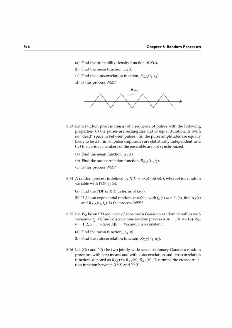
316 Chapter 8 Random Processes
(a) Find the probability density function of X(t).
(b) Find the mean function, µX(t).
(c) Find the autocorrelation function, RX,X(t1, t2).
(d) Is this process WSS?
. . .. . .
s(t)
t
1
−1 1 2
8.13 Let a random process consist of a sequence of pulses with the followingproperties: (i) the pulses are rectangular and of equal duration, (withno “dead” space in between pulses), (ii) the pulse amplitudes are equallylikely to be ±1, (iii) all pulse amplitudes are statistically independent, and(iv) the various members of the ensemble are not synchronized.
(a) Find the mean function, µX(t).
(b) Find the autocorrelation function, RX,X(t1, t2).
(c) Is this process WSS?
8.14 A random process is defined by X(t) = exp(−At)u(t), where A is a randomvariable with PDF, fA(a).
(a) Find the PDF of X(t) in terms of fA(a).
(b) If A is an exponential random variable, with fA(a) = e−au(a), find µX(t)and RX,X(t1, t2). Is the process WSS?
8.15 Let Wn be an IID sequence of zero-mean Gaussian random variables withvariance σ 2
W . Define a discrete time random process X[n] = pX[n−1]+Wn,n = 1, 2, 3, . . ., where X[0] = W0 and p is a constant.
(a) Find the mean function, µX[n].(b) Find the autocorrelation function, RX,X[n1, n2].
8.16 Let X(t) and Y(t) be two jointly wide sense stationary Gaussian randomprocesses with zero means and with autocorrelation and crosscorrelationfunctions denoted as RXX(τ ), RYY(τ ), RXY(τ ). Determine the crosscorrela-tion function between X2(t) and Y2(t).

Exercises 317
8.17 If X(t) is a wide sense stationary Gaussian random process, find the cross-correlation between X(t) and X3(t) in terms of the autocorrelation functionRXX(τ ).
8.18 Two zero mean discrete random processes, X[n] and Y[n], are statisticallyindependent. Let a new random process be Z[n] = X[n] + Y[n]. Let theautocorrelation functions for X[n] and Y[n] be
RXX[k] =(
12
)|k|, RYY[k] =
(13
)|k|.
Find RZZ[k]. Plot all three autocorrelation functions (you may want to useMATLAB to help).
8.19 Consider a discrete time wide sense stationary random processes whoseautocorrelation funcion is of the form
RXX[k] = a|k|, where |a| < 1.
Assume this process has zero-mean. Is the process ergodic in the mean?
8.20 Let X(t) be a wide sense stationary random process that is ergodic in themean and the autocorrelation. However, X(t) is not zero-mean. Let Y(t) =CX(t), where C is a random variable independent of X(t) and C is notzero-mean. Show that Y(t) is not ergodic in the mean or the autocorrelation.
8.21 Prove that the family of differential equations
ddt
PX(0; t) + λPX(0; t) = 0,
ddt
PX(i; t) + λPX(i; t) = λPX(i − 1; t), i = 1, 2, 3, . . . ,
leads to the Poisson distribution
PX(i; t) = (λt)i
i! e−λt.
8.22 Consider a Poisson counting process with arrival rate λ.
(a) Suppose it is observed that there is exactly one arrival in the timeinterval [0, to). Find the PDF of that arrival time.
(b) Now suppose there were exactly two arrivals in the time interval[0, to). Find the joint PDF of those two arrival times.
Can you extend these results to an arbitrary number, n, of arrivals?

318 Chapter 8 Random Processes
8.23 Let X(t) be a Poisson counting process with arrival rate λ. Find Pr(N(t) =k|N(t + τ ) = m), where τ > 0 and m ≥ k.
8.24 Let X(t) be a WSS random process with mean µX and autocorrelationfunction RXX(τ ). Consider forming a new process according to
Y(t) = X(t + to) − X(t)to
.
(a) Find the mean function of Y(t).
(b) Find the autocorrelation function of Y(t). Is Y(t) WSS?
8.25 Let Xi(t), i = 1, 2, . . . , n be a sequence of independent Poisson countingprocesses with arrival rates λi. Show that the sum of all of these Poissonprocesses,
X(t) =n∑
i=1
Xi(t),
is itself a Poisson process. What is the arrival rate of the sum process?
8.26 A workstation is used until it fails and is then sent out for repair. Thetime between failures, or the length of time the workstation functionsuntil it needs repair, is a random variable T. Assume the times betweenfailures, T1, T2, . . . Tn, of the workstations available are independent ran-dom variables that are identically distributed. For t > 0, let the number ofworkstations that have failed be N(t).
(a) If the time between failures of each workstation has an exponentialPDF, then what type of process is N(t)?
(b) Assume that you have just purchased 10 new workstations and thateach has a 90-day warranty. If the mean time between failures (MTBF)is 250 days, what is the probability that at least one workstation willfail before the end of the warranty period?
8.27 Suppose the arrival of calls at a switchboard is modeled as a Poissonprocess with the rate of calls per minute being λa = 0. 1.
(a) What is the probability that the number of calls arriving in a 10-minuteinterval is less than 10?
(b) What is the probability that the number of calls arriving in a 10-minuteinterval is less than 10 if λa = 10?

MATLAB Exercises 319
(c) Assuming λa = 0. 1, what is the probability that one call arrives duringthe first 10-minute interval and two calls arrive during the second10-minute interval?
8.28 Model lightning strikes to a power line during a thunderstorm as a Poissonimpulse process. Suppose the number of lightning strikes in time intervalt has a mean rate of arrival given by s, which is one strike per 3 minutes.
(a) What is the expected number of lightning strikes in 1 minute? in10 minutes?
(b) What is the average time between lightning strikes?
8.29 Suppose the power line in the previous problem has an impulse responsethat may be approximated by h(t) = te−atu(t), where a = 10 sec−1.
(a) What does the shot noise on the power line look like? Sketch a possiblemember function of the shot noise process.
(b) Find the mean function of the shot noise process.
(c) Find the autocorrelation function of the shot noise process.
8.30 A shot noise process with random amplitudes is defined by
X(t) =∞∑
i=1
Aih(t − Si),
where the Si are a sequence of points from a Poisson process and the Aiare IID random variables that are also independent of the Poisson points.
(a) Find the mean function of X(t).
(b) Find the autocorrelation function of X(t).
MATLAB Exercises8.31 You are given a member function of a random process as y(t) = 10 sin(2π t+
π/2 where the amplitude is in volts. Quantize the amplitude of y(t) into21 levels with the intervals ranging from −10. 5 to 10.5 in 1-volt steps.Consider 100 periods of y(t) and let t take on discrete values given by nts
where ts = 5 msec. Construct a histogram of y(t).

320 Chapter 8 Random Processes
8.32 Write a MATLAB program to generate a Bernoulli process X[n] for whicheach time instant of the process is a Bernoulli random variable withPr(X[n] = 1) = 0. 1 and Pr(X[n] = 0) = 0. 9. Also, the process is IID(i.e., X[n] is independent of X[m] for all m �= n). Once you have created theprogram to simulate X[n], then create a counting process Y[n] that countsthe number of occurrences of X[m] = 1 in the interval m ∈ [0, n]. Plotmember functions of each of the two processes.
8.33 Let Wn, n = 0, 1, 2, 3, . . . be a sequence of IID zero-mean Gaussian randomvariables with variance σ 2
W = 1.
(a) Write a MATLAB program to generate the process
X[n] = 12 X[n − 1] − 1
4 X[n − 2] − 14 X[n − 3] + Wn,
where X[0] = W0 and X[n] = 0 for n < 0.(b) Estimate the mean function of this process by generating a large num-
ber of realizations of the random process and computing the samplemean.
(c) Compute the time averaged mean of the process from a single real-ization. Does this seem to give the same result as the ensemble meanestimated in part (b)?
8.34 A certain random process is created as a sum of a large number, n, ofsinusoids with random frequencies and random phases,
X(t) =n∑
k=1
cos(2πFkt + θk),
where the random phases θk are IID and uniformly distributed over(0, 2π ), and the random frequencies are given by Fk = fo + fd cos(βk),where the βk are IID and uniformly distributed over (0, 1). (Note: Thesetypes of processes occur in the study of wireless communication systems.)For this exercise, we will take the constants fo and fd to be fo = 25 Hz andfd = 10 Hz, while we will let the number of terms in the sum be n = 32.
(a) Write a MATLAB program to generate realizations of this randomprocess.
(b) Assuming the process is stationary and ergodic, use a single realizationto estimate the first order PDF of the process, fX(x).
(c) Assuming the process is stationary and ergodic, use a single realizationto estimate the mean of the process, µX .

MATLAB Exercises 321
(d) Assuming the process is stationary and ergodic, use a single realizationto estimate the autocorrelation function of the process, RXX(τ ).
8.35 Write a MATLAB program to generate a shot noise process with
h(t) = b(at) exp(−at)u(t),
where a = 1012 sec−1 and the constant b is chosen so that q = ∫h(t) dt. For
this program, assume that carriers cross the depletion region at a rate of1013 per second. Plot a member function of this random process.

Markov Processes 9
In this chapter we study a class of random processes that possess a certain char-acteristic that could crudely be described as memoryless. These processes appearin numerous applications, including queuing systems, computer communicationsnetworks, biological systems, and a wide array of other applications. As a resultof their frequent occurrence, these processes have been studied extensively anda wealth of theory exists to solve problems related to these processes. We makeno attempt to give an exhaustive treatment here, but rather present some of thefundamental concepts involving Markov processes.
9.1 Definition and Examples of MarkovProcesses
DEFINITION 9.1: A random process, X(t), is said to be a Markov process if forany time instants, t1 < t2 < · · · < tn < tn+1, the random process satisfies
FX(X(tn+1) ≤ xn+1∣∣ X(tn) = xn, X(tn−1) = xn−1, . . . , X(t1) = x1)
= FX(X(tn+1) ≤ xn+1∣∣ X(tn) = xn). (9.1)
To understand this definition, we interpret tn as the present time so that tn+1 rep-resents some point in the future and t1, t2, . . . , tn−1 represent various points in thepast. The Markovian property then states that given the present, the future is inde-pendent of the past. Or, in other words, the future of the random process dependsonly on where it is now and not on how it got there.
323

324 Chapter 9 Markov Processes
EXAMPLE 9.1: A classical example of a continuous time Markov pro-cess is the Poisson counting process studied in the previous chapter. LetX(t) be a Poisson counting process with rate λ. Then its probability massfunction satisfies
Pr(X(tn+1) = xn+1∣∣ X(tn) = xn, X(tn−1) = xn−1, . . . , X(t1) = x1)
=
0 xn+1 < xn
(λ(tn+1 − tn))xn+1−xn
(xn+1 − xn)! e−λ(tn+1−tn) xn+1 ≥ xn
.
Clearly, this is independent of {X(tn−1) = xn−1, . . . , X(t1) = x1}. In fact,the Markovian property must be satisfied because of the independentincrements assumption of the Poisson process.
To start with, we will focus our attention on discrete-valued Markov processesin discrete time, better known as Markov chains. Let X[k] be the value of theprocess at time instant k. Since the process is discrete-valued, X[k] ∈ {x1, x2, x3, . . .}and we say that if X[k] = xn, then the process is in state n at time k. A Markovchain is described statistically by its transition probabilities which are defined asfollows.
DEFINITION 9.2: Let X[k] be a Markov chain with states {x1, x2, x3, . . .}, then theprobability of transitioning from state i to state j in one time instant is
pi, j = Pr(X[k + 1] = j|X[k] = i). (9.2)
If the Markov chain has a finite number of states, n, then it is convenient to definea transition probability matrix,
P =
p1, 1 p1, 2 · · · p1, n
p2, 1 p2, 2 · · · p2, n
pn, 1 pn, 2 · · · pn, n
. (9.3)
One can encounter processes where the transition probabilities vary with time andhence need to be explicitly written as a function of k (e.g., pi, j, k), but we do notconsider such processes in this text and henceforth it is assumed that transitionprobabilities are independent of time.
9.1 Definition and Examples of Markov Processes 325
EXAMPLE 9.2: Suppose every time a child buys a kid’s meal at hisfavorite fast food restaurant, he receives one of four superhero actionfigures. Naturally, the child wants to collect all four action figures andso he regularly eats lunch at this restaurant in order to complete thecollection. This process can be described by a Markov chain. In thiscase, let X[k] ∈ {0, 1, 2, 3, 4} be the number of different action figuresthat the child has collected after purchasing k meals. Assuming eachmeal contains one of the four superheroes with equal probability andthat the action figure in any meal is independent of what is containedin any previous or future meals, then the transition probability matrixeasily works out to be
P =
0 1 0 0 00 1/4 3/4 0 00 0 1/2 1/2 00 0 0 3/4 1/40 0 0 0 1
.
Initially (before any meals are bought), the process starts in state 0(the child has no action figures). When the first meal is bought, theMarkov chain must move to state 1 since no matter which action figureis contained in the meal, the child will now have one superhero. Hence,p0, 1 = 1 and p0, j = 0 for all j �= 1. If the child has one distinct actionfigure, when he buys the next meal he has a 25 percent chance of receiv-ing a duplicate and a 75 percent chance of getting a new action figure.Hence, p1, 1 = 1/4, p1, 2 = 3/4, and p1, j = 0 for j �= 1, 2. Similar logic isused to complete the rest of the matrix. The child might be interestedin knowing the average number of lunches he needs to buy until hiscollection is completed. Or, maybe the child has saved up only enoughmoney to buy 10 lunches and wants to know what his chances are ofcompleting the set before running out of money. We will develop thetheory needed to answer such questions.
The transition process of a Markov chain can also be illustrated graphically usinga state diagram. Such a diagram is illustrated in Figure 9.1 for the Markov chainin Example 9.2. In the figure, each directed arrow represents a possible transitionand the label on each arrow represents the probability of making that transition.Note that for this Markov chain, once we reach state 4, we remain there forever.This type of state is referred to as an absorbing state.

326 Chapter 9 Markov Processes
0 1 2 3 41
1/2 3/4
1/4
1/4
1/23/4
1
Figure 9.1 State diagram for the Markov chain of Example 9.2.
EXAMPLE 9.3: (The Gambler’s Ruin Problem) Suppose a gamblerplays a certain game of chance (e.g., blackjack) against the “house.”Every time the gambler wins the game, he increases his fortune by oneunit (say, a dollar) and every time he loses, his fortune decreases by oneunit. Suppose the gambler wins each game with probability p and loseswith probability q = 1−p. Let Xn represent the amount of the gambler’sfortune after playing the game n times. If the gambler ever reaches thestate Xn = 0, the gambler is said to be “ruined” (he has lost all of hismoney). Assuming that the outcome of each game is independent of allothers, the sequence xn, n = 0, 1, 2, . . . forms a Markov chain. The statetransition matrix is of the form
P =
1 0 0 0 0 . . .
q 0 p 0 0 . . .
0 q 0 p 0 . . .
0 0 q 0 p . . .
. . . . . . . . .
.
The state transition diagram for the gambler’s ruin problem is shownin Figure 9.2. One might then be interested in determining how long it
0 1 2 3 4 5 . . .1q
q q q q q
p p p p p
(a)
p p p p p p
0 1 2 3 4 5 . . .1q
q q q q q
bb-1 1p
q
(b)
Figure 9.2 State transition diagram for Example 9.3 (The Gambler’s Ruin Problem), withone absorbing state (a) and with two absorbing states (b).

9.1 Definition and Examples of Markov Processes 327
might take before the gambler is ruined (enters the zero state). Is ruininevitable for any p, or if the gambler is sufficiently proficient at thegame, can he avoid ruin indefinitely? A more realistic alternative tothis model is one where the house also has a finite amount of money.Suppose the gambler starts with d dollars and the house has b−d dollarsso that between the two competitors there is a total of b dollars in thegame. Now if the gambler ever gets to the state 0 he is ruined, while ifhe gets to the state b he has “broken the bank” (i.e., the house is ruined).Now the Markov chain has two absorbing states as shown in part (b) ofthe figure. It would seem that sooner or later the gambler must have arun of bad luck sufficient to send him to the 0 state (i.e., ruin) or a run ofgood luck which will cause him to enter the state b (i.e., break the bank).It would be interesting to find the probabilities of each of these events.
The previous example is one of a class of Markov chains known as randomwalks. Random walks are often used to describe the motion of a particle. Of course,there are many applications that can be described by a random walk that do notinvolve the movement of a particle, but it is helpful to think of such a particle whendescribing such a Markov chain. In one dimension, a random walk is a Markovchain whose states are the integers and whose transition probabilities satisfy pi, j = 0for any j �= i−1, i, i+1. In other words, at each time instant, the state of the Markovchain can either increase by one, stay the same, or decrease by one. If pi, i+1 = pi, i−1,then the random walk is said to be symmetric, whereas if pi, i+1 �= pi, i−1 the randomwalk is said to have drift. Often the state space of the random walk will be a finiterange of integers, n, n + 1, n + 1, . . . , m − 1, m (for m > n), in which case the statesn and m are said to be boundaries, or barriers. The gambler’s ruin problem is anexample of a random walk with absorbing boundaries, where pn, n = pm, m = 1.Once the particle reaches the boundary, it is absorbed and remains there forever.We could also construct a random walk with reflecting boundaries, in which casepn, n+1 = pm, m−1 = 1. That is, whenever the particle reaches the boundary, it isalways reflected back to the adjacent state.
EXAMPLE 9.4: (A Queueing System) A common example of Markovchains (and Markov processes in general) is that of queueing systems.Consider, for example, a taxi stand at a busy airport. A line of taxis,which for all practical purposes can be taken to be infinitely long, isavailable to serve travelers. Customers wanting a taxi enter a queueand are given a taxi on a first come, first serve basis. Suppose it takesone unit of time (say, a minute) for the customer at the head of the

328 Chapter 9 Markov Processes
queue to load himself and his luggage into a taxi. Hence, during eachunit of time, one customer in the queue receives service and leaves thequeue while some random number of new customers enter the end ofthe queue. Suppose at each time instant, the number of new customersarriving for service is described by a discrete distribution (p0, p1, p2, . . .),where pk is the probability of k new customers. For such a system, thetransition probability matrix of the Markov chain would look like
P =
p0 p1 p2 p3 . . .
p0 p1 p2 p3 . . .
0 p0 p1 p2 . . .
0 0 p0 p1 . . .
. . . . . . . . .
.
The manager of the taxi stand might be interested in knowing theprobability distribution of the queue length. If customers have towait too long, they may get dissatisfied and seek other forms oftransportation.
EXAMPLE 9.5: (A Branching Process) Branching processes are com-monly used in biological studies. Suppose a certain species of organismhas a fixed lifespan (one time unit). At the end of its lifespan, the nthorganism in the species produces a number of offspring described bysome random variable, Yn, whose sample space is the set of nonnega-tive integers. Also, assume that the number of offspring produced byeach organism is independent and identically distributed (IID). Then,Xk, the number of organisms in the species during the kth generationis a random variable that depends only on the number of organisms inthe previous generation. In particular, if Xk = i, then Xk+1 = ∑i
n=1 Yn.The transition probability is then
pi, j = Pr(Xk+1 = j∣∣ Xk = i) = Pr
i∑
n=1
Yn = j
.
Let HY(z) be the probability generating function of the random variableYn (i.e., HY(z) = ∑∞
i=0 Pr(Yn = i)zi). Then, due to the IID nature of the Yn,∑i
n=1 Yn will have a probability generating function given by [HY(z)]i.Hence, the transition probability, pi, j, will be given by the coefficient ofzj in the power series expansion of [HY(z)]i.

9.2 Calculating Transition and State Probabilities in Markov Chains 329
EXAMPLE 9.6: (A Genetic Model) Suppose a gene contains n units. Ofthese units, i are mutant and n − i are normal. Every time a cell doubles,the n units double and each of the two cells receives a gene composedof n units. After doubling, there is a pool of 2n units of which 2i aremutant. These 2n units are grouped into two sets of n units randomly.As we trace a single line of descent, the number of mutant units in eachgene forms a Markov chain. Define the kth gene to be in state i (whereXk = i) if it is composed of i mutant and n − i normal units. It is notdifficult to show that, given Xk = i,
pi, j = Pr(Xk+1 = j∣∣ Xk = i) =
(2ij
)(2n − 2i
n − j
)
(2nn
) .
9.2 Calculating Transition and StateProbabilities in Markov Chains
The state transition probability matrix of a Markov chain gives the probabilitiesof transitioning from one state to another in a single time unit. It will be useful toextend this concept to longer time intervals.
DEFINITION 9.3: The n-step transition probability for a Markov chain is
p(n)i, j = Pr(Xk+n = j
∣∣ Xk = i). (9.4)
Also, define an n-step transition probability matrix P(n) whose elements are then-step transition probabilities just described in Equation 9.4.
Given the one-step transition probabilities, it is straightforward to calculate higherorder transition probabilities using the following result.
THEOREM 9.1: (Chapman-Kolmogorov Equation)
p(n)i, j =
∑
k
p(m)i, k p(n−m)
k, j , for any m = 0, 1, 2, . . . , n (9.5)

330 Chapter 9 Markov Processes
PROOF: First, condition on the event that in the process of transitioning fromstate i to state j, the Markov chain passes through state k at some intermediatepoint in time. Then, using the principle of total probability,
Pr(Xl+n = j∣∣Xl = i)=
∑
k
Pr(Xl+n = j∣∣Xl = i, Xl+m =k)Pr(Xl+m =k
∣∣Xk = i). (9.6)
Using the Markov property, the expression reduces to the desired form:
Pr(Xl+n = j∣∣ Xl = i) =
∑
k
Pr(Xl+n = j∣∣ Xl+m = k) Pr(Xl+m = k
∣∣ Xk = i). (9.7)
�
This result can be written in a more compact form using transition probabilitymatrices. It is easily seen that the Chapman-Kolmogorov equations can be writtenin terms of the n-step transition probability matrices as
P(n) = P(m)P(n−m). (9.8)
Then, starting with the fact that P(1) = P, it follows that P(2) = P(1)P(1) = P2, andusing induction, it is established that
P(n) = Pn. (9.9)
Hence, we can find the n-step transition probability matrix through matrixmultiplication. If n is large, it may be more convenient to compute Pn via eigen-decomposition. The matrix P can be expanded as P = U�U−1, where � isthe diagonal matrix of eigenvalues and U is the matrix whose columns are thecorresponding eigenvectors. Then
Pn = U� nU−1. (9.10)
Another quantity of interest is the probability distribution of the Markov chainat some time instant k. If the initial probability distribution of the Markov chain isknown, then the distribution at some later point in time can easily be found. Letπj(k) = Pr(Xk = j) and π (k) be the row vector whose jth element is πj(k). Then
πj(k) = Pr(Xk = j) =∑
i
Pr(Xk = j∣∣ X0 = i) Pr(X0 = i) =
∑
i
p(k)i, j πi(0), (9.11)
or in vector form,
π (k) = π (0)Pk. (9.12)
EXAMPLE 9.7: (Continuation of Example 9.2) Recall in Example 9.2the child who purchased kid’s meals at his favorite restaurant in order

9.2 Calculating Transition and State Probabilities in Markov Chains 331
to collect a set of four superhero action figures. Initially, before anymeals are purchased, the child has no action figures and so the initialprobability distribution is π (0) = 1, 0, 0, 0, 0). Repeated application ofEquation 9.12 with the probability transition matrix given in Example9.2 results in
π (1) = (0, 1, 0, 0, 0),
π (2) = (0, 1/4, 3/4, 0, 0),
π (3) = (0, 1/16, 9/16, 3/8, 0),
π (4) = (0, 1/64, 21/64, 9/16, 3/32),
π (5) = (0, 1/256, 45/256, 75/128, 15/64),
π (6) = (0, 1/1024, 93/1024, 135/256, 195/512),
and so on. It is to be expected that if the child buys enough meals, he willeventually complete the collection (i.e., get to state 4) with probabilityapproaching unity. This can be easily verified analytically by calculatingthe limiting form of Pk as k → ∞. Recall that for this example, P is atriangular matrix and hence its eigenvalues are simply the diagonalentries. Thus, the diagonal matrix of eigenvalues is
� =
0 0 0 0 00 1/4 0 0 00 0 1/2 0 00 0 0 3/4 00 0 0 0 1
.
It should be clear that limk→∞ �k is a matrix with all zero entries exceptthe one in the lower-right corner, which is equal to one. Using MATLAB(or some other math package) to calculate the corresponding matrix ofeigenvectors, it is found that
limk→∞
Pk = U(
limk→∞
�k)
U−1 =
0 0 0 0 10 0 0 0 10 0 0 0 10 0 0 0 10 0 0 0 1
.
Then, using the initial distribution of π (0) = (1, 0, 0, 0, 0), the statedistribution as k → ∞ works out to be
π = limk→∞
π (k) = limk→∞
π (0)Pk = [0 0 0 0 1].

332 Chapter 9 Markov Processes
In Example 9.6, it was seen that as k → ∞, the k-step transition probabilitymatrix approached that of a matrix whose rows were all identical. In that case, thelimiting product limk→∞ π (0)Pk is the same regardless of the initial distributionπ (0). Such a Markov chain is said to have a unique steady state distribution, π .It should be emphasized that not all Markov chains have a steady state distribu-tion. For example, the Poisson counting process of Example 9.1 clearly does not,since any counting process is a monotonic, nondecreasing function of time and,hence, it is expected that the distribution should skew towards larger values astime progresses.
This concept of a steady state distribution can be viewed from the perspectiveof stationarity. Suppose that at time k, the process has some distribution, π (k). Thedistribution at the next time instant is then π (k+1) = π (k)P. If π (k) = π (k+1), thenthe process has reached a point where the distribution is stationary (independentof time). This stationary distribution, π , must satisfy the relationship
π = πP. (9.13)
In other words, π (if it exists) is the left eigenvector of the transition probabilitymatrix P, that corresponds to the eigenvalue λ = 1. The next example shows thatthis eigenvector is not always unique.
EXAMPLE 9.8: (The Gambler’s Ruin Revisited) Suppose a certaingambler has $5 and plays against another player (the house). The gam-bler decides that he will play until he either doubles his money or losesit all. Suppose the house has designed this game of chance so that thegambler will win with probability p = 0. 45 and the house will win withprobability q = 0. 55. Let Xk be the amount of money the gambler hasafter playing the game k times. The transition probability matrix for thisMarkov chain is
P =
1 0 0 0 0 0 0 0 0 0 00. 55 0 0. 45 0 0 0 0 0 0 0 0
0 0. 55 0 0. 45 0 0 0 0 0 0 00 0 0. 55 0 0. 45 0 0 0 0 0 00 0 0 0. 55 0 0. 45 0 0 0 0 00 0 0 0 0. 55 0 0. 45 0 0 0 00 0 0 0 0 0. 55 0 0. 45 0 0 00 0 0 0 0 0 0. 55 0 0. 45 0 00 0 0 0 0 0 0 0. 55 0 0. 45 00 0 0 0 0 0 0 0 0. 55 0 0. 450 0 0 0 0 0 0 0 0 0 1
.

9.2 Calculating Transition and State Probabilities in Markov Chains 333
This matrix has (two) repeated eigenvalues of λ = 1, and the corre-sponding eigenvectors are [1 0 0 0 0 0 0 0 0 0 0] and [0 0 0 0 0 0 0 0 0 0 1].Note that any linear combination of these will also be an eigenvector.Hence, any vector of the form [p 0 0 0 0 0 0 0 0 0 1 − p] is a left eigen-vector of P and therefore there is no unique stationary distribution forthis Markov chain. For this example, the limiting form of the state dis-tribution of the Markov chain depends on the initial distribution. Thelimiting form of Pk can be easily found to be
limk→∞
Pk =
1 0 0 0 0 0 0 0 0 0 00. 9655 0 0 0 0 0 0 0 0 0 0. 03450. 9233 0 0 0 0 0 0 0 0 0 0. 07670. 8717 0 0 0 0 0 0 0 0 0 0. 12830. 8087 0 0 0 0 0 0 0 0 0 0. 19130. 7317 0 0 0 0 0 0 0 0 0 0. 26830. 6376 0 0 0 0 0 0 0 0 0 0. 36240. 5225 0 0 0 0 0 0 0 0 0 0. 47750. 3819 0 0 0 0 0 0 0 0 0 0. 61810. 2101 0 0 0 0 0 0 0 0 0 0. 7899
0 0 0 0 0 0 0 0 0 0 1
.
Using the initial distribution π (0) = [0 0 0 0 0 1 0 0 0 0 0] (that is, thegambler starts off in state 5), then it is seen that the steady state distri-bution is limk→∞ π (k) = [0.7317 0 0 0 0 0 0 0 0 0 0.2683]. So, when thegambler starts with $5, he has about a 73 percent chance of losing all ofhis money and about a 27 percent chance of doubling his money.
As seen in Example 9.7, with some Markov chains, the limiting form of Pk (ask → ∞) does not necessarily converge to a matrix whose rows are all identical.In that case, the limiting form of the state distribution will depend on the startingdistribution. In the case of the gambler’s ruin problem, we probably could haveguessed this behavior. If the gambler had started with very little money, we wouldexpect him to end up in the state of ruin with very high probability; whereas, if thegambler was very wealthy and the house had very little money, we would expecta much greater chance of the gambler eventually breaking the house. Accordingly,our intuition tells us that the probability distribution of the gambler’s ultimate stateshould depend on the starting state.
In general, there are several different manners in which a Markov chain’s statedistribution can behave as k → ∞. In some cases, limk→∞ π (k) does not exist. Suchwould be the case when the process tends to oscillate between two or more states.A second possibility, as in Example 9.7, is that limk→∞ π (k) does in fact converge

334 Chapter 9 Markov Processes
to a fixed distribution, but the form of this limiting distribution depends on thestarting distribution. The last case is when limk→∞ π (k) = π . That is, the statedistribution converges to some fixed distribution, π , and the form of π is inde-pendent of the starting distribution. Here, the transition probability matrix, P,will have a single (not repeated) eigenvalue at λ = 1, and the correspondingeigenvector (properly normalized) will be the steady state distribution, π . Fur-thermore, the limiting form of Pk will be one whose rows are all identical andequal to the steady state distribution, π . In the next section, we look at some con-ditions that must be satisfied for the Markov chain to achieve a unique steady statedistribution.
EXAMPLE 9.9: In this example, we provide the MATLAB codeto simulate the distribution of the queue length of the taxi standdescribed in Example 9.4. For this example, we take the number ofarrivals per time unit, X, to be a Poisson random variable whose
PMF is
PX(k) = λke−λ
k! .
Recall that in the taxi stand, one customer is served per time unit (assumingthere is at least one customer in the queue waiting to be served). The followingcode can be used to estimate and plot the PMF of the queue length. Theaverage queue length was also calculated to be 3.36 customers for an arrivalrate of λ = 0. 85 customers per time unit. Figure 9.3 shows a histogram of thePMF of the queue length for the same arrival rate.
N=10000; % Length of simulation.a=0.85; % Arrival rate.k=[0:10];Poisson=zeros(size(k)); % Calculate Poisson PMF.for m=k
Poisson(m+1)=a.∧m*exp(-a)./factorial(m);endqueue(1)=0; % Initial queue size.for n=1:N
x=rand(1);arrivals=sum(x>cumsum(Poisson)); % Poisson RV.departures=queue(n)>0;queue(n+1)=queue(n)+arrivals-departures; % Current queue length.
endmean_queue_length=sum(queue)/length(queue) % Compute average queue
length.bins=[0:25]

9.3 Characterization of Markov Chains 335
0 5 10 15 20 250
0.02
0.04
0.06
0.08
0.1
0.12
0.14
0.16
0.18
0.2
Queue length
Pro
babi
lity
mas
s fu
nctio
n
Figure 9.3 Histogram of the queue length for the Taxi stand of Example 9.4 assuming aPoisson arrival process with an average arrival rate of 0.85 arrivals per time unit.
y=hist(queue,bins);
PMF=y/N; % Estimate PMF.
bar(bins,PMF) % Plot results.
axis([min(bins)-1 max(bins)+1 0 1.1*max(PMF)])
9.3 Characterization of Markov Chains
Using the methods presented in the previous sections, calculating the steady statedistribution of a Markov chain requires performing an eigendecomposition of thetransition probability matrix, P. If the number of states in the Markov chain is large(or infinite), performing the required linear algebra may be difficult (or impossible).Hence, it would be useful to seek alternative methods to determine if a steady statedistribution exists, and if so, to calculate it. To develop the necessary theory, wemust first proceed through a sequence of definitions and classifications of the statesof a Markov chain.
DEFINITION 9.4: State j is accessible from state i if for some finite n, p(n)i, j > 0. This
simply means that if the process is in state i, it is possible for the process to get to

336 Chapter 9 Markov Processes
state j in a finite amount of time. Furthermore, if state j is accessible from state iand state i is accessible from state j, then the states i and j are said to communicate. Itis common to use the shorthand notation i ↔ j to represent the relationship “statei communicates with state j.”
The states of any Markov chain can be divided into sets or classes of states whereall the states in a given class communicate with each other. It is possible for theprocess to move from one communicating class of states to another, but once thattransition is made, the process can never return to the original class. If it did, thetwo classes would communicate with each other and hence would be a part of asingle class.
DEFINITION 9.5: A Markov chain for which all of the states are part of a singlecommunicating class is called an irreducible Markov chain. Also, the correspondingtransition probability matrix is called an irreducible matrix.
The examples in Section 9.1 can be used to help illustrate these concepts. Forboth processes in Examples 9.1 and 9.2, none of the states communicate with anyother states. This is a result of the fact that both processes are counting processesand it is therefore impossible to go backward in the chain of states. Hence, if j > i,state j is accessible from state i but state i is not accessible from state j. As a result,for any counting process, all states form a communication class of their own. Thatis, the number of classes is identical to the number of states. In the gambler’s ruinproblem of Example 9.3, the two absorbing states do not communicate with anyother state since it is impossible ever to leave an absorbing state, while all the statesin between communicate with each other. Hence, this Markov chain has threecommunicating classes. The two absorbing states each form a class to themselves,while the third class consists of all the states in between.
The queueing system (i.e., taxi stand) of Example 9.4 represents a Markov chainwhere all states communicate with each other, and hence that Markov chain isirreducible. For the branching process of Example 9.5, all states communicate witheach other except the state 0, which represents the extinction of the species, whichpresumably is an absorbing state. The genetic model of Example 9.6 is similar tothe gambler’s ruin problem in that the Markov chain has two absorbing states atthe endpoints, while everything in between forms a single communicating class.
DEFINITION 9.6: The period of state i, d(i), is the greatest common divisor of allintegers n ≥ 1 such that p(n)
i, i > 0. Stated another way, d(i) is the period of state i ifany transition from state i to itself must occur in a number of steps that is a multipleof d(i). Furthermore, a Markov chain for which all states have a period of d(i) = 1is called an aperiodic Markov chain.

9.3 Characterization of Markov Chains 337
Most Markov chains are aperiodic. The class of random walks is an exception.Suppose a Markov chain defined on the set of integers has transition probabilitiesthat satisfy
pi, j =
p j = i + 1
1 − p j = i − 1
0 otherwise
. (9.14)
Then each state will have a period of 2. If we add absorbing boundaries to therandom walk, then the absorbing states are not periodic because for the absorbingstates, p(n)
i, i = 1 for all n and hence the period of an absorbing state is 1. It is left asan exercise for the reader (see Exercise 9.18) to establish the fact that the period isa property of a class of communicating states. That is, if i ↔ j then d(i) = d(j) andhence all states in the same class must have the same period.
DEFINITION 9.7: Let f (n)i, i be the probability that given a process is in state i, the
first return to state i will occur in exactly n steps. Mathematically,
f (n)i, i = Pr(Xk+n = i, Xk+m �= i for m = 1, 2, . . . , n − 1
∣∣ Xk = i). (9.15)
Also, define fi, i to be the probability that the process will eventually return to state i.The probability of eventual return is related to the first return probabilities by
fi, i =∞∑
n=1
f (n)i, i . (9.16)
It should be noted that the first return probability f (n)i, i is not the same thing as
the n-step transition probability, but the two quantities are related. To develop thisrelationship, it is observed that
p(n)i, i =
n∑
m=0
Pr({Xk+n = i}, {first return to state i occurs in m steps}∣∣ Xk = i) (9.17)
=n
∑
m=0
Pr(Xk+n = i∣∣ Xk+m = i) Pr(first return to state i occurs in m steps
∣∣ Xk = i)
(9.18)
=n
∑
m=0
p(n−m)i, i f (m)
i, i , n = 1, 2, 3, . . . . (9.19)
In the Equations 9.17–9.19, p(0)i, i is taken to be equal to 1 and f (0)
i, i is taken to be equal
to 0. Given the n-step transition probabilities, p(n)i, i , one could solve the preceding

338 Chapter 9 Markov Processes
system of equations for the first return probabilities. However, since the previoussystem is a convolution, this set of equations may be easier to solve using frequencydomain techniques. Define the generating functions1
Pi, i(z) =∞∑
n=0
p(n)i, i zn, (9.20)
Fi, i(z) =∞∑
n=0
f (n)i, i zn. (9.21)
It is left as an exercise for the reader (see Exercise 9.19) to demonstrate that thesetwo generating functions are related by
Pi, i(z) − 1 = Pi, i(z)Fi, i(z). (9.22)
This relationship provides an easy way to compute the first return probabilitiesfrom the n-step transition probabilities. Note that if the transition probability matrixis known, then calculating the generating function, Pi, i(z), is straightforward. Recallthat Pn = U� nU−1, and hence if [U]i, j is the element in the ith row and jth columnof U, then
p(n)i, i =
∑
j
[U]i, j�n[U−1]j, i. (9.23)
Forming the generating function from this equation results in
Pi, i(z) =∞∑
n=0
p(n)i, i zn =
∞∑
n=0
∑
j
[U]i, j(�z) n[U−1]j, i
=∑
j
[U]i, j
( ∞∑
n=0
(�z)n
)
[U−1]j, i
=∑
j
[U]i, j
( ∞∑
n=0
(�z)n
)
[U−1]j, i
=∑
j
[U]i, j(I − �z)−1[U−1]j, i. (9.24)
In other words, Pi, i(z) is the element in the ith row and ith column of the matrixU(I − �z)−1U−1.
1Note that these generating functions are not necessarily probability generating functionsbecause the sequences involved are not necessarily probability distributions.

9.3 Characterization of Markov Chains 339
DEFINITION 9.8: The ith state of a Markov chain is transient if fi, i < 1 and recurrentif fi, i = 1. Since fi, i represents the probability of the process eventually returningto state i given that it is in state i, the state is transient if there is some nonzeroprobability that it will never return, and the state is recurrent if the process musteventually return with probability 1.
THEOREM 9.2: State i of a Markov chain is recurrent if and only if
∞∑
n=1
p(n)i, i = ∞. (9.25)
Since this sum represents the expected number of returns to state i, it follows thata state is recurrent if and only if the expected number of returns is infinite.
PROOF: First, note that fi, i = ∑∞n=1 f (n)
i, i = lim z→1 Fi, i(z). From Equation 9.22, thiswould imply that
limz→1
Pi, i(z) − 1 = limz→1
Pi, i(z)fi, i. (9.26)
As a result,
limz→1
Pi, i(z) =∞∑
n=1
p(n)i, i = 1
1 − fi, i. (9.27)
If state i is transient, then fi, i < 1 and hence,
∞∑
n=1
p(n)i, i < ∞,
whereas if state i is recurrent,
fi, i = 1 and∞∑
n=1
p(n)i, i = ∞.
�
We leave it to the reader (see Exercise 9.21) to verify that recurrence is a classproperty. That is, if one state in a communicating class is recurrent, then all arerecurrent, and if one is transient, then all are transient.
EXAMPLE 9.10: Consider a random walk on the integers (both positiveand negative) that initially starts at the origin (X0 = 0). At each time
340 Chapter 9 Markov Processes
instant, the process either increases by 1 with probability p or decreasesby 1 with probability 1 − p:
pi, j =
p if j = i + 1
1 − p if j = i − 1
0 otherwise
.
First note that this Markov chain is periodic with period 2 and hencep(n)
i, i = 0 for any odd n. For even n, given the process is in state i, theprocess will be in state i again n time instants later if during those timeinstants the process increases n/2 times and decreases n/2 times. Thisprobability follows a binomial distribution so that
p(n)i, i =
(n
n/2
)
pn/2(1 − p)n/2, for even n.
To determine if the states of this random walk are recurrent or transient,we must determine whether or not the series
∞∑
n=1
p(2n)i, i =
∞∑
n=1
(2nn
)
(p(1 − p))n
converges. To help make this determination, the identity∞∑
n=1
(2nn
)
xn = 1√1 − 4x
− 1, |x| < 1/4
is used. This identity can easily be verified by expanding the binomial onthe right-hand side in powers of x and confirming (after a little algebra)that the coefficients of the power series expansion do take on the desiredform. Applying this identity results in
∞∑
n=1
p(2n)i, i = 1
√
1 − 4p(1 − p)− 1.
Note that for a probability p, 4p(1 − p) ≤ 1 with equality if and onlyif p = 1/2. Hence, the series converges and all states are transientif p �= 1/2, while if p = 1/2 the series diverges and all states arerecurrent.
DEFINITION 9.9: The mean time to first return for a recurrent state i of a Markovchain is
µi =∞∑
n=1
nf (n)i, i . (9.28)
9.3 Characterization of Markov Chains 341
If the state is transient, then the mean time to first return must be infinite, sincewith some nonzero probability, the process will never return.
DEFINITION 9.10: A recurrent state is referred to as null recurrent if µi = ∞,while the state is positive recurrent if µi < ∞.
The mean time to first return of a recurrent state is related to the steady stateprobability of the process being in that state. To see this, define a sequence ofrandom variables T1, T2, T3, . . ., where Tm represents the time between the (m−1)thand mth returns to the state i. That is, suppose that Xk = i for some time instant kwhich is sufficiently large so that the process has pretty much reached steady state.The process then returns to state i at time instants k+T1, k+T1 +T2, k+T1 +T2 +T3,and so on. Over some period of time where the process visits state i exactly n times,the fraction of time the process spends in state i can be written as
fraction of time process is in state i = nn
∑
j=1
Tj
= 1
1n
n∑
j=1
Tj
. (9.29)
As n → ∞ (assuming the process is ergodic), the left-hand side of the previousequation becomes the steady state probability that the process is in state i, πi.Furthermore, due to the law of large numbers, the denominator of the right-handside converges to µi. This proves the following key result.
THEOREM 9.3: For an irreducible, aperiodic, recurrent Markov Chain, the steadystate distribution is unique and is given by
πi = 1µi
. (9.30)
Note that if a state is positive recurrent then πi > 0, while if a state is null recurrentthen πi = 0. Note that for any transient state, µi = ∞ and as a result, πi = 0.
EXAMPLE 9.11: Continuing with the random walk from the previousexample, the generating function for the n-step transition probabilitiesis found to be
Pi, i(z) =∞∑
n=0
p(n)i, i zn =
∞∑
n=0
(2nn
)
(p(1 − p))nz2n = 1√
1 − 4p(1 − p)z2.

342 Chapter 9 Markov Processes
Using the relationship Pi, i(z) − 1 = Pi, i(z)Fi, i(z), the generating functionfor the first return probabilities is
Fi, i(z) = 1 −√
1 − 4p(1 − p)z2.
Since the random walk is recurrent only for p = 1/2, we consider onlythat case so that Fi, i(z) = 1 −
√
1 − z2. The mean time to first return canbe found directly from the generating function.
µi =∞∑
n=1
nf (n)i, i = lim
z→1
ddz
Fi, i(z) = limz→1
z√
1 − z2= ∞
Thus, when the transition probabilities of the random walk are balancedso that all states are recurrent, then the mean time to first return is infiniteand, in fact, all states are null recurrent.
9.4 Continuous Time Markov Processes
In this section, we investigate Markov processes where the time variable is continu-ous. In particular, most of our attention will be devoted to the so-called birth-deathprocesses which are a generalization of the Poisson counting process studied inthe previous chapter. To start with, consider a random process X(t) whose statespace is either finite or countable infinite so that we can represent the states of theprocess by the set of integers, X(t) ∈ {. . . , −3, −2, −1, 0, 1, 2, 3, . . .}. Any process ofthis sort that is a Markov process has the interesting property that the time betweenany change of states is an exponential random variable. To see this, define Ti tobe the time between the ith and the (i + 1)th change of state and let hi(t) be thecomplement to its CDF, hi(t) = Pr(Ti > t). Then, for t > 0, s > 0,
hi(t + s) = Pr(Ti > t + s) = Pr(Ti > t + s, Ti > s) = Pr(Ti > t + s∣∣ Ti > s) Pr(Ti > s).
(9.31)
Due to the Markovian nature of the process, Pr(Ti > t + s∣∣ Ti > s) = Pr(Ti > t),
and hence the previous equation simplifies to
hi(t + s) = hi(t)hi(s). (9.32)
The only function which satisfies this type of relationship for arbitrary t ands is an exponential function of the form hi(t) = e−ρit for some constant ρi.

9.4 Continuous Time Markov Processes 343
Furthermore, for this function to be a valid probability, the constant ρi must not benegative. From this, the PDF of the time between change of states is easily foundto be fTi (t) = ρie−ρitu(t).
As with discrete time Markov chains, the continuous time Markov process canbe described by its transition probabilities.
DEFINITION 9.11: Define pi, j(t) = Pr(X(to + t) = j|X(to) = i) to be the transi-tion probability for a continuous time Markov process. If this probability does notdepend on to, then the process is said to be a homogeneous Markov process.
Unless otherwise stated, we assume for the rest of this chapter that all continuoustime Markov processes are homogeneous. The transition probabilities, pi, j(t), aresomewhat analogous to the n-step transition probabilities used in the study ofdiscrete time processes and as a result, these probabilities satisfy a continuous timeversion of the Chapman-Kolmogorov equations:
pi, j(t + s) =∑
k
pi, k(t)pk, j(s), for t, s > 0. (9.33)
One of the most commonly studied class of continuous time Markov processesis the birth-death process. These processes get their name from applications inthe study of biological systems, but they are also commonly used in the study ofqueueing theory, and many other applications. The birth-death process is similarto the discrete time random walk studied in the previous section in that when theprocess changes states, it either increases by 1 or decreases by 1. As with the Poissoncounting process, the general class of birth-death processes can be described by thetransition probabilities over an infinitesimal period of time, �t. For a birth-deathprocess,
pi, j(�t) =
λi�t + o(�t) if j = i + 1
µi�t + o(�t) if j = i − 1
1 − (λi + µi)�t + o(�t) if j = i
o(�t) if j �= i − 1, i, i + 1
. (9.34)
The parameter λi is called the birth rate, while µi is the death rate when the processis in state i. In the context of queueing theory, λi and µi are referred to as the arrivaland departure rates, respectively.
Similar to what was done with the Poisson counting process, by letting s = �tin Equation 9.33 and then applying the infinitesimal transition probabilities, a setof differential equations can be developed that will allow us to solve for the general
344 Chapter 9 Markov Processes
transition probabilities. From Equation 9.33,
pi, j(t + �t) =∑
k
pi, k(t)pk, j(�t)
= (λj−1�t)pi, j−1(t) + (1 − (λj + µj)�t)pi, j(t) + (µj+1�t)pi, j+1(t) + o(�t). (9.35)
Rearranging terms and dividing by �t produces
pi, j(t + �t) − pi, j(t)
�t= λj−1pi, j−1(t) − (λj + µj)pi, j(t) + µj+1pi, j+1(t) + o(�t)
�t.
(9.36)
Finally, passing to the limit as �t → 0 results in
ddt
pi, j(t) = λj−1pi, j−1(t) − (λj + µj)pi, j(t) + µj+1pi, j+1(t). (9.37)
This set of equations is referred to as the forward Kolmogorov equations. One canfollow a similar procedure (see Exercise 9.24) to develop a slightly different set ofequations known as the backward Kolmogorov equations:
ddt
pi, j(t) = λipi+1, j(t) − (λi + µi)pi, j(t) + µipi−1, j(t). (9.38)
For all but the simplest examples, it is very difficult to find a closed form solutionfor this system of equations. However, the Kolmogorov equations can lend someinsight into the behavior of the system. For example, consider the steady statedistribution of the Markov process. If a steady state exists, we would expect thatas t → ∞, pi, j(t) → πj independent of i and also that dpi, j(t)/(dt) → 0. Pluggingthese simplifications into the forward Kolmogorov equations leads to
λj−1πj−1 − (λj + µj)πj + µj+1πj+1 = 0. (9.39)
These equations are known as the global balance equations. From them, the steadystate distribution can be found (if it exists). The solution to the balance equationsis surprisingly easy to obtain. First, we rewrite the difference equation in the moresymmetric form
λjπj − µj+1πj+1 = λj−1πj−1 − µjπj. (9.40)
Next, assume that the Markov process is defined on the states j = 0, 1, 2, . . .. Thenthe previous equation must be adjusted for the end point j = 0 (assuming µ0 = 0which merely states that there can be no deaths when the population’s size is zero)according to
λ0π0 − µ1π1 = 0. (9.41)

9.4 Continuous Time Markov Processes 345
Combining Equations 9.40 and 9.41 results in
λjπj − µj+1πj+1 = 0, j = 0, 1, 2, . . . , (9.42)
which leads to the simple recursion
πj+1 = λj
µj+1πj, j = 0, 1, 2, . . . , (9.43)
whose solution is given by
πj = π0
j∏
i=1
λi−1
µi, j = 1, 2, 3, . . . . (9.44)
This gives the πj in terms of π0. In order to determine π0, the constraint that the πjmust form a distribution is imposed.
∞∑
j=0
πj = 1 ⇒ π0 = 1
1 +∞∑
j=1
j∏
i=1
λi−1
µi
. (9.45)
This completes the proof of the following theorem.
THEOREM 9.4: For a Markov birth-death process with birth rate λn, n = 0, 1, 2, . . .,and death rate µn, n = 1, 2, 3, . . ., the steady state distribution is given by
πk = limt→∞ pi, k(t) =
k∏
i=1
λi−1
µi
1 +∞∑
j=1
j∏
i=1
λi−1
µi
. (9.46)
If the series in the denominator diverges, then πk = 0 for any finite k. This indicatesthat a steady state distribution does not exist. Likewise, if the series converges, theπk will be nonzero, resulting in a well-behaved steady state distribution.
EXAMPLE 9.12: (The M/M/1 Queue) In this example, we consider thebirth-death process with constant birth rate and constant death rate. Inparticular, we take
λn = λ, n = 0, 1, 2, . . . and µ0 = 0, µn = µ, n = 1, 2, 3, . . . .

346 Chapter 9 Markov Processes
This model is commonly used in the study of queueing systems and, inthat context, is referred to as the M/M/1 queue. In this nomenclature,the first “M” refers to the arrival process as being Markovian, the second“M” refers to the departure process as being Markovian, and the “1”is the number of servers. So this is a single server queue, where theinterarrival time of new customers is an exponential random variablewith mean 1/λ and the service time for each customer is exponentialwith mean 1/µ. For the M/M/1 queueing system, λi−1/µi = λ/µ forall i so that
1 +∞∑
j=1
j∏
i=1
λi−1
µi=
∞∑
j=0
(λ
µ
)j
= 11 − λ/µ
for λ < µ.
The resulting steady state distribution of the queue size is then
πk = (λ/µ)k
11 − λ/µ
= (1 − λ/µ)(λ/µ)k, k = 0, 1, 2, . . . , for λ < µ.
Hence, if the arrival rate is less than the departure rate, the queue sizewill have a steady state. It makes sense that if the arrival rate is greaterthan the departure rate, then the queue size will tend to grow withoutbound.
EXAMPLE 9.13: (The M/M/∞ Queue) Next suppose the last exampleis modified so that there are an infinite number of servers available tosimultaneously provide service to all customers in the system. In thatcase, there are no customers ever waiting in line, and the process X(t)now counts the number of customers in the system (receiving service) attime t. As before, we take the arrival rate to be constant λn = λ, but nowthe departure rate needs to be proportional to the number of customersin service, µn = nµ. In this case, λi−1/µi = λ/(iµ) and
1 +∞∑
j=1
j∏
i=1
λi−1
µi= 1 +
∞∑
j=1
j∏
i=1
λ
iµ= 1 +
∞∑
j=1
(λ/µ)j
j! = eλ/µ.
Note that the series converges for any λ and µ, and hence the M/M/∞queue will always have a steady state distribution given by
πk = (λ/µ)k
k! e−λ/µ.

9.4 Continuous Time Markov Processes 347
EXAMPLE 9.14: This example demonstrates one way to simulatethe M/M/1 queueing system of Example 9.12. One realization ofthis process as produced by the code that follows is illustratedin Figure 9.4. In generating the figure, we use an average arrival
rate of λ = 20 customers per hour and an average service time of 1/µ = 2minutes. This leads to the condition λ < µ and the M/M/1 queue exhibitsstable behavior. The reader is encouraged to run the program for the casewhen λ > µ to observe the unstable behavior (the queue size will tend togrow continuously over time).
a=20; % Arrival rate (customers/hour).
b=30; % Departure rate (1/b=avg service
time).
N=25; % Number of arrivals in simulation.
X=-log(rand(1,N))/a; % Random interarrival times.
X=cumsum(X); % Random arrival times.
Y=-log(rand(1,N))/b; % Service times for each customer.
serv_start=X(1); % First customer starts service
% immediately upon arrival.
0 0.1 0.2 0.3 0.4 0.5 0.6 0.7 0.8 0.9
0
0.5
1
1.5
2
2.5
3
3.5
4
Time (hours)
Que
ue s
ize
Figure 9.4 Simulated realization of the birth-death process for M/M/1 queueing systemof Example 9.12.

348 Chapter 9 Markov Processes
Z(1)=serv_start+Y(1); % Departure time of first
customer.
for k=2:N % kth customer.
serv_start=max([Z(k-1), X(k)]); % Beginning of service
time.
Z(k)=serv_start+Y(k); % End of service time.
end
% Construct data to plot graph of queue size vs. time.
xaxis=[0, X(1)]; % Vector of points for
the M/M/1.
% Birth-death process
yaxis=[0, 0]; % Vector of queue sizes at
points in preceding vector.
qs=1; % Current queue size.
X=X(2:length(X));
while length(X)>0
if X(1)<Z(1) % Next point is arrival.
qs=qs+1; % Increase queue size.
xaxis=[xaxis xaxis(length(xaxis)) X(1)];
yaxis=[yaxis qs qs];
X=X(2:length(X));
else % Next point is departure.
qs=qs-1; % decrease queue size
xaxis=[xaxis xaxis(length(xaxis)) Z(1)];
yaxis=[yaxis qs qs];
Z=Z(2:length(Z));
end
end
plot(xaxis,yaxis) % Plot realization of
% birth-death process.
xlabel(‘time (hours)’);
ylabel(‘queue size’)
If the birth-death process is truly modeling the size of a population of someorganism, then it would be reasonable to consider the case when λ0 = 0. That is,when the population size reaches zero, no further births can occur. In that case, thespecies is extinct and the state X(t) = 0 is an absorbing state. A fundamental ques-tion would then be, Is extinction a certain event, and if not what is the probabilityof the process being absorbed into the state of extinction? Naturally the answer tothis question would depend on the starting population size. Let qi be the probabil-ity that the process eventually enters the absorbing state, given that it is initially

9.4 Continuous Time Markov Processes 349
in state i. Note that if the process is currently in state i, after the next transition, thebirth-death process must be either in state i − 1 or state i + 1. The time to the nextbirth, Bi, is a random variable with an exponential distribution with a mean of 1/λi,while the time to the next death is an exponential random variable, Di, with a meanof 1/µi. Hence, the process will transition to state i + 1 if Bi < Di, otherwise it willtransition to state i − 1. The reader can easily verify that Pr(Bi < Di) = λi/(λi +µi).The absorption probability can then be written as
qi = Pr (absorption | in state i)
= Pr (absorption, next state is i + 1|in state i)
+ Pr (absorption, next state is i − 1| in state i)
= Pr (absorption | in state i + 1) Pr (next state is i + 1| in state i)
+ Pr (absorption | in state i − 1) Pr (next state is i − 1| in state i)
= qi+1λi
λi + µi+ qi−1
µi
λi + µi, i = 1, 2, 3, . . . . (9.47)
This provides a recursive set of equations that can be solved to find the absorptionprobabilities. To solve this set of equations, we rewrite them as
qi+1 − qi = µi
λi(qi − qi−1), i = 1, 2, 3, . . . . (9.48)
After applying this recursion repeatedly and using the fact that q0 = 1,
qi+1 − qi = (q1 − 1)i
∏
j=1
µj
λj. (9.49)
Summing this equation from i = 1, 2, . . . , n results in
qn+1 − q1 = (q1 − 1)n
∑
i=1
i∏
j=1
µj
λj. (9.50)
Next, suppose that the series on the right-hand side of the previous equationdiverges as n → ∞. Since the qi are probabilities, the left-hand side of the equa-tion must be bounded, which implies that q1 = 1. Then from Equation 9.49, it isdetermined that qn must be equal to one for all n. That is, if
∞∑
i=1
i∏
j=1
µj
λj= ∞, (9.51)

350 Chapter 9 Markov Processes
then absorption will eventually occur with probability 1 regardless of the startingstate. If q1 < 1 (absorption is not certain), then the preceding series must convergeto a finite number. It is expected in that case that as n → ∞, qn → 0. Passing to thelimit as n → ∞ in Equation 9.50 then allows a solution for q1 of the form
q1 =
∞∑
i=1
i∏
j=1
µj
λj
1 +∞∑
i=1
i∏
j=1
µj
λj
. (9.52)
Furthermore, the general solution for the absorption probability is
qn =
∞∑
i=n
i∏
j=1
µj
λj
1 +∞∑
i=1
i∏
j=1
µj
λj
. (9.53)
EXAMPLE 9.15: Consider a population model where both the birth anddeath rates are proportional to the population, λn = nλ, µn = nµ. Forthis model,
∞∑
i=1
i∏
j=1
µj
λj=
∞∑
i=1
i∏
j=1
µ
λ=
∞∑
i=1
(µ
λ
)i = µ/λ
1 − µ/λ= µ
λ − µfor λ > µ.
Hence, if λ < µ, the series diverges and the species will eventually reachextinction with probability 1. If λ > µ,
∞∑
i=n
i∏
j=1
µj
λj=
∞∑
i=n
(µ
λ
)i = (µ/λ)n
1 − µ/λ,
and the absorption (extinction) probabilities are
qn =(µ
λ
)n, n = 1, 2, 3, . . . .
Continuous time Markov processes do not necessarily need to have a discreteamplitude as in the previous examples. In the following, we discuss a class of

9.4 Continuous Time Markov Processes 351
continuous time, continuous amplitude Markov processes. To start with, it is notedthat for any time instants t0 < t1 < t2, the conditional PDF of a Markov processmust satisfy the Chapman-Kolmogorov equation
f (x2, t2|x0, t0) =∫ ∞
−∞f (x2, t2|x1, t1)f (x1, t1|x0, t0) dx1. (9.54)
This is just the continuous amplitude version of Equation 9.33. Here we use thenotation f (x2, t2|x1, t1) to represent the conditional probability density of the pro-cess X(t2) at the point x2 conditioned on X(t1) = x1. Next, suppose we interpretthese time instants as t0 = 0, t1 = t, and t2 = t + �t. In this case, we interpretx2 − x1 = �x as the the infinitesimal change in the process that occurs during theinfinitesimal time instant �t and f (x2, t2|x1, t1) is the PDF of that increment.
Define ��x(ω) to be the characteristic function of �x = x2 − x1:
��x(ω) = E[ejω�x] =∫ ∞
−∞ejω(x2−x1)f (x2, t + �t|x1, t) dx2. (9.55)
We note that the characteristic function can be expressed in a Taylor series as
��x(ω) =∞∑
k=0
Mk(x1, t)k! (jω)k, (9.56)
where Mk(x1, t) = E[(x2 − x1)k∣∣ (x1, t)] is the kth moment of the increment
�x. Taking inverse transforms of this expression, the conditional PDF can beexpressed as
f (x2, t + �t|x1, t) =∞∑
k=0
Mk(x1, t)k! (−1)k ∂k
∂xk2
(δ(x2 − x1)). (9.57)
Inserting this result into the Chapman-Kolmogorov equation, Equation 9.54,results in
f (x2, t + �t|x0, t0) =∞∑
k=0
(−1)k
k!∫ ∞
−∞Mk(x1, t)
∂k
∂xk2
δ(x2 − x1)f (x1, t|x0, t0) dx1
=∞∑
k=0
(−1)k
k!∂k
∂xk2
[Mk(x2, t)f (x2, t|x0, t0)]
= f (x2, t|x0, t0) +∞∑
k=1
(−1)k
k!∂k
∂xk2
[Mk(x2, t)f (x2, t|x0, t0)]. (9.58)

352 Chapter 9 Markov Processes
Subtracting f (x2, t|x0, t0) from both sides of this equation and dividing by �tresults in
f (x2, t + �t|x0, t0) − f (x2, t|x0, t0)�t
=∞∑
k=1
(−1)k
k!∂k
∂xk2
[Mk(x2, t)
�tf (x2, t|x0, t0)
]
.
(9.59)
Finally, passing to the limit as �t → 0 results in the partial differential equation
∂
∂tf (x, t|x0, t0) =
∞∑
k=1
(−1)k
k!∂k
∂xk[Kk(x, t)f (x, t|x0, t0)], (9.60)
where the function Kk(x, t) is defined as
Kk(x, t) = lim�t→0
E[(X(t + �t) − X(t))k|X(t)]�t
. (9.61)
For many processes of interest, the PDF of an infinitesimal increment can be accu-rately approximated from its first few moments, and hence we take Kk(x, t) = 0 fork > 2. For such processes, the PDF must satisfy
∂
∂tf (x, t|x0, t0) = − ∂
∂x(K1(x, t)f (x, t|x0, t0)) + 1
2∂2
∂x2 (K2(x, t)f (x, t|x0, t0)). (9.62)
This is known as the (one-dimensional) Fokker-Planck equation and is used exten-sively in diffusion theory to model the dispersion of fumes, smoke, and similarphenomena.
In general, the Fokker-Planck equation is notoriously difficult to solve and doingso is well beyond the scope of this text. Instead, we consider a simple special casewhere the functions K1(x, t) and K2(x, t) are constants, in which case the FokkerPlanck equation reduces to
∂
∂tf (x, t|x0, t0) = −2c
∂
∂x(f (x, t|x0, t0)) + D
∂2
∂x2 (f (x, t|x0, t0)), (9.63)
where in diffusion theory, D is known as the coefficient of diffusion and c is thedrift. This equation is used in models that involve the diffusion of smoke or otherpollutants in the atmosphere, the diffusion of electrons in a conductive medium,the diffusion of liquid pollutants in water and soil, and the diffusion of plasmas.This equation can be solved in several ways. Perhaps one of the easiest methodsis to use Fourier transforms. This is explored further in the exercises where thereader is asked to show that (taking x0 = 0 and t0 = 0) the solution to this diffusionequation is
f (x, t|x0 = 0, t0 = 0) = 1√4πDt
exp
(
− (x − 2ct)2
4Dt
)
. (9.64)

9.4 Continuous Time Markov Processes 353
That is, the PDF is Gaussian with a mean and variance that changes with time. Thebehavior of this process is explored in the next example.
EXAMPLE 9.16: In this example, we model the diffusion of smokefrom a forest fire that starts in a National Park at time t = 0 andlocation x = 0. The smoke from the fire drifts in the positive xdirection due to wind blowing at 10 miles per hour, and the dif-
fusion coefficient is 1 square mile per hour. The probability density functionis given in Equation 9.64. We provide a three-dimensional rendition of thisfunction in Figure 9.5 using the following MATLAB program.
c=10; % Drift.
D=1; % Diffusion coefficient.
tpoints=[0.25, 0.5, 1, 1.5, 2]; % Time samples.
x=[0:0.1:50]; % x-axis.
0 5 10 15 20 25 30 35 40 45 500
0.5
f(x,
0.25
)
0 5 10 15 20 25 30 35 40 45 500
0.5
f(x,
0.5)
0 5 10 15 20 25 30 35 40 45 500
0.5
f(x,
1)
0 5 10 15 20 25 30 35 40 45 500
0.5
f(x,
1.5)
0 5 10 15 20 25 30 35 40 45 500
0.5
f(x,
2)
x (miles)
Figure 9.5 Observations of the PDF at different time instants showing the drift anddispersion of smoke for Example 9.16.

354 Chapter 9 Markov Processes
for k=1:length(tpoints)
t=tpoints(k); % Set t.
pdf(k,:)=exp(-(x-2*c*t).∧2/(4*D*t))/sqrt(4*pi*D*t);% f(x,t).
subplot(5,1,k)
plot(x,pdf(k,:)) % Plot PDF.
axis([0 max(x) 0 1.1*max(max(pdf))])
s=num2str(t);
leftstr=‘f(x,’;
rightstr=‘)’;
txt=[leftstr s rightstr];
ylabel(txt)
end
xlabel(‘x (miles)’)
9.5 Engineering Application: A ComputerCommunication Network
Consider a local area computer network where a cluster of nodes is connected by acommon communications line. Suppose for simplicity that these nodes occasionallyneed to transmit a message of some fixed length (or, number of packets). Also,assume that the nodes are synchronized so that time is divided into slots, each ofwhich is sufficiently long to support one packet. In this example, we consider arandom access protocol known as slotted Aloha. Messages (packets) are assumedto arrive at each node according to a Poisson process. Assuming there are a totalof n nodes, the packet arrival rate at each node is assumed to be λ/n so that thetotal arrival rate of packets is fixed at λ packets/slot. In slotted Aloha, every timea new packet arrives at a node, that node attempts to transmit that packet duringthe next slot. During each slot, one of three events can occur: (1) no node attemptsto transmit a packet, in which case the slot is said to be idle; (2) exactly one nodeattempts to transmit a packet, in which case the transmission is successful; or (3)more than one node attempts to transmit a packet, in which case a collision is saidto have occurred.
All nodes involved in a collision will need to retransmit their packets, but ifthey all retransmit during the next slot, then they will continue to collide and thepackets will never be successfully transmitted. All nodes involved in a collisionare said to be backlogged until their packet is successfully transmitted. In the

9.5 Engineering Application: A Computer Communication Network 355
slotted Aloha protocol, each backlogged node chooses to transmit during the nextslot with probability p (and hence chooses not to transmit during the next slotwith probability 1 − p). Viewed in an alternative manner, every time a collisionoccurs, each node involved waits a random amount of time until they attemptretransmission, where that random time follows a geometric distribution.
This computer network can be described by a Markov chain, Xk = number ofbacklogged nodes at the end of the kth slot. To start with, we evaluate the transitionprobabilities of the Markov chain, pi, j. Assuming that there are an infinite numberof nodes (or a finite number of nodes, each of which could store an arbitrary numberof backlogged packets in a buffer), we note that
Pr(m backlogged nodes attempt to transmit|Xk = n) =(
nm
)
pm(1 − p)n−m, (9.65)
Pr(m new arrivals|Xk = n) = λm
m! e−λ. (9.66)
Using these equations, it is straightforward to determine that the transitionprobabilities are given by
pi, j =
0 for j < i − 1
ip(1 − p)i−1e−λ for j = i − 1
(1 + λ(1 − p)i − ip(1 − p)i−1)e−λ for j = i
(1 − (1 − p)i)λe−λ for j = i + 1
λj−i
(j − i)! e−λ for j > i + 1
. (9.67)
In order to get a feeling for the steady state behavior of this Markov chain, wedefine the drift of the chain in state i as
di = E[Xk+1|Xk = i] − i. (9.68)
Given that the chain is in state i, if the drift is positive, then the number of back-logged nodes will tend to increase; whereas, if the drift is negative, the number ofbacklogged nodes will tend to decrease. Crudely speaking, a drift of zero repre-sents some sort of equilibrium for the Markov chain. Given the preceding transitionprobabilities a, the drift works out to be
di = λ − (1 − p)i−1e−λ[ip + λ(1 − p)]. (9.69)
Assuming that p � 1, then we can use the approximations (1−p) ≈ 1 and (1−p)i ≈e−ip to simplify the expression for the drift:
di ≈ λ − g(i)e−g(i), where g(i) = λ + ip. (9.70)
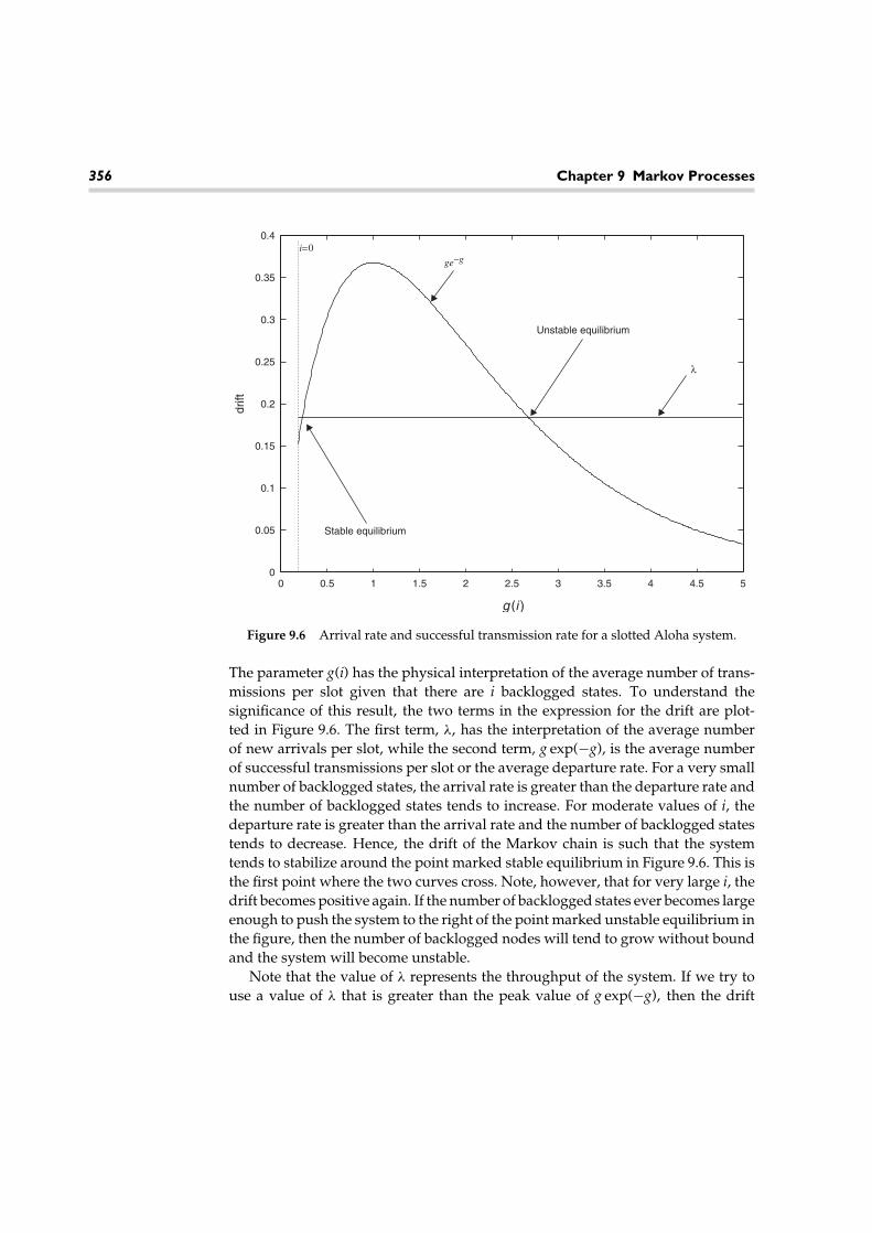
356 Chapter 9 Markov Processes
0 0.5 1 1.5 2 2.5 3 3.5 4 4.5 50
0.05
0.1
0.15
0.2drift
0.25
0.3
0.35
0.4
g (i )
i=0
ge−g
Unstable equilibrium
Stable equilibrium
λ
Figure 9.6 Arrival rate and successful transmission rate for a slotted Aloha system.
The parameter g(i) has the physical interpretation of the average number of trans-missions per slot given that there are i backlogged states. To understand thesignificance of this result, the two terms in the expression for the drift are plot-ted in Figure 9.6. The first term, λ, has the interpretation of the average numberof new arrivals per slot, while the second term, g exp(−g), is the average numberof successful transmissions per slot or the average departure rate. For a very smallnumber of backlogged states, the arrival rate is greater than the departure rate andthe number of backlogged states tends to increase. For moderate values of i, thedeparture rate is greater than the arrival rate and the number of backlogged statestends to decrease. Hence, the drift of the Markov chain is such that the systemtends to stabilize around the point marked stable equilibrium in Figure 9.6. This isthe first point where the two curves cross. Note, however, that for very large i, thedrift becomes positive again. If the number of backlogged states ever becomes largeenough to push the system to the right of the point marked unstable equilibrium inthe figure, then the number of backlogged nodes will tend to grow without boundand the system will become unstable.
Note that the value of λ represents the throughput of the system. If we try touse a value of λ that is greater than the peak value of g exp(−g), then the drift

9.6 Engineering Application: A Telephone Exchange 357
will always be positive and the system will be unstable from the beginning. Thismaximum throughput occurs when g(i) = 1 and has a value of λmax = 1/e. Bychoosing an arrival rate less than λmax, we can get the system to operate near thestable equilibrium, but sooner or later, we will get a string of bad luck and thesystem will drift into the unstable region. The lower the arrival rate, the longer itwill take (on average) for the system to become unstable, but at any arrival rate, thesystem will eventually reach the unstable region. Hence, slotted Aloha is inherentlyan unstable protocol. As a result, various modifications have been proposed thatexhibit stable behavior.
9.6 Engineering Application: A TelephoneExchange
Consider a base station in a cellular phone system. Suppose calls arrive at the basestation according to a Poisson process with some arrival rate λ. These calls areinitiated by a mobile unit within the cell served by that base station. Furthermore,suppose each call has a duration that is an exponential random variable with somemean, 1/µ. The base station has some fixed number of channels, m, that can be usedto service the demands of the mobiles in its cell. If all m channels are being used,any new call that is initiated cannot be served and the call is said to be blocked. Weare interested in calculating the probability that when a mobile initiates a call, thecustomer is blocked.
Since the arrival process is memoryless and the departure process is memo-ryless, the number of calls being serviced by the base station at time t, X(t), is abirth-death Markov process. Here, the arrival rate and departure rates (given thereare n channels currently being used) are given by
λn ={
λ 0 ≤ n < m
0 n = m, µn = nµ, 0 ≤ n ≤ m. (9.71)
The steady state distribution of this Markov process is given by Equation 9.46. Forthis example, the distribution is found to be
πn =
n∏
i=1
λi−1
µi
1 +m
∑
j=1
j∏
i=1
λi−1
µi
=1n!
(λ
µ
)n
m∑
j=0
1j!
(λ
µ
)j. (9.72)

358 Chapter 9 Markov Processes
The blocking probability is just the probability that when a call is initiated, it findsthe system in state m. In steady state, this is given by πm and the resulting blockingprobability is the so-called Erlang-B formula,
Pr (blocked call) =1
m!(
λ
µ
)m
m∑
j=0
1j!
(λ
µ
)j. (9.73)
This equation is plotted in Figure 9.7 for several values of m. The horizontal axisis the ratio of λ/µ which is referred to in the telephony literature as the trafficintensity. As an example of the use of this equation, suppose a certain base stationhad 60 channels available to service incoming calls. Furthermore, suppose eachuser initiated calls at a rate of 1 call per 3 hours and calls had an average duration
10–1
Traffic intensity (Erlangs)
Blo
ckin
g pr
obab
ility
From left to right m = 1,2,3,4,5,6,8,10,12,15,20,25,30,40,50,60,70,80,90,100
10 0
10 0
10−1
10−2
10−3
10 1 10 2
Figure 9.7 The Erlang-B formula.

Exercises 359
of 3 minutes (0.05 hours). If a 2 percent probability of blocking is desired, thenfrom Figure 9.7 we determine that the system can handle a traffic intensity ofapproximately 50 Erlangs. Note that each user generates an intensity of
λ
µ= 1/(3 hour)
1/(0.05 hour)= 1
60Erlangs. (9.74)
Hence, a total of 50 ∗ 60 = 3, 000 mobile users per cell could be supported whilestill maintaining a 2 percent blocking probability.
Concluding Remarks
This chapter has covered a class of random process that can be described asmemoryless, with emphasis on Markov Processes. While the material is difficult,it is nonetheless important in that it is applicable to numerous applications suchas queuing systems and computer communications networks, as illustrated by thelast two engineering applications examples. The reader is encouraged to masterthis material by completing as many of the exercises that follow as possible.
Exercises9.1 Consider a two-state Markov chain with a general transition probability
matrix
P =[
1 − p pq 1 − p
]
,
where 0 < p, q < 1. Find an expression for the n-step transition probabilitymatrix, Pn.
9.2 For the general two-state Markov chain of Exercise 9.1, suppose the statesare called 0 and 1. Furthermore, suppose Pr(X0 = 0) = s and Pr(X0 = 1) =1 − s.
(a) Find Pr(X1 = 0, X2 = 1).(b) Find Pr(X1 = 1|X0 = 0, X2 = 0).(c) Find Pr(X2 = X1). Is it the same as Pr(X1 = X0)?
9.3 For a Markov chain, prove or disprove the following statement:
Pr(Xk = ik|Xk+1 = ik+1, Xk+2 = ik+2, . . . , Xk+m = ik+m)
= Pr(Xk = ik|Xk+1 = ik+1).

360 Chapter 9 Markov Processes
9.4 A square matrix P is called a stochastic matrix if all of its elements satisfy0 ≤ pi, j ≤ 1 and, furthermore,
∑
j
pi, j = 1 for all i.
Every stochastic matrix is the transition probability matrix for someMarkov chain; however, not every stochastic matrix is a valid two-steptransition probability matrix. Prove that a 2 × 2 stochastic matrix is a validtwo-step transition probability matrix for a two-state Markov chain if andonly if the sum of the diagonal elements is greater than or equal to 1.
9.5 A random waveform is generated as follows. The waveform starts at 0voltage. Every ts seconds, the waveform switches to a new voltage level.If the waveform is at a voltage level of 0 volts, it may move to +1 volt withprobability p, or it may move to −1 volt with probability q = 1−p. Once thewaveform is at +1 (or −1), the waveform will return (with probability 1)to 0 volts at the next switching instant.
(a) Model this process as a Markov Chain. Describe the states of the systemand give the transition probability matrix.
(b) Determine whether each state is periodic or aperiodic. If periodic,determine the period of each state.
(c) For each instant of time, determine the PDF for the value of thewaveform.
9.6 Model the diffusion of electrons and holes across a potential barrier in anelectronic device as follows. We have n black balls (electrons) in urn A andn whiteballs (holes) in urn B. An experimental outcome selects randomlyone ball from each urn. The ball from urn A is placed in urn B and thatfrom urn B is placed in A. Let the state of the process be the number ofblack balls in urn A. (By knowing the number of black balls in urn A, weknow the composition of both urns.) Let k denote the state of the process.Find the transition probabilities, pi, j.
9.7 A PCM waveform has the two states +1 and 0. Suppose the transitionmatrix is
P =[
0. 5 0. 50. 25 0. 75
]
.
The initial value of the waveform is determined by the flip of a coin, withthe outcome of a head corresponding to +1 and a tail to 0.

Exercises 361
(a) What is the probability that the waveform will be at +1 after one stepif the coin is a fair coin?
(b) Find the same probability if the coin is biased such that a head occurswith probability 1/3.
(c) Repeat the problem for two steps.
9.8 A student takes this course at period 1 on Monday, Wednesday, and Fri-day. Period 1 starts at 7:25 A.M. Consequently, the student sometimesmisses class. The student’s attendance behavior is such that she attendsclass depending only on whether or not she went to the last class. If sheattended class on one day, then she will go to class the next time it meetswith probability 1/2. If she did not go to one class, then she will go to thenext class with probability 3/4.
(a) Find the transition matrix P.(b) Find the probability that if she went to class on Wednesday, she will
attend class on Friday.(c) Find the probability that if she went to class on Monday, she will attend
class on Friday.(d) Does the Markov chain described by this transition matrix have a
steady state distribution? If so, find that distribution.
9.9 A three-state Markov chain has the following transition matrix:
P =
0. 25 0. 5 0. 250. 4 0. 6 01 0 0
.
(a) Does this Markov chain have a unique steady state probability vector?If so, find it.
(b) What is the approximate value of p(100)1, 3 ? What interpretation do you
give to this result?(c) What is the probability that after the third step you are in state 3 if the
initial state probability vector is (1/3 1/3 1/3)?
9.10 The three letters C, A, and T represent the states of a word-generatingsystem. Let the initial state probability vector be (1/3 1/3 1/3) for thethree letters, respectively. The transition matrix is given as
C A T
P =CAT
0. 1 0. 7 0. 20. 6 0. 1 0. 30. 1 0. 8 0. 1
.

362 Chapter 9 Markov Processes
What is the probability of generating a proper three-letter English wordafter two transitions from the initial state?
9.11 Two students play the following game. Two dice are tossed. If the sumof the numbers showing is less than 7, student A collects a dollar fromstudent B. If the total is greater than 7, then student B collects a dollar fromstudent A. If a 7 appears, then the student with the fewest dollars collectsa dollar from the other. If the students have the same amount, then nodollars are exchanged. The game continues until one student runs out ofdollars. Let student A’s number of dollars represent the states. Let eachstudent start with 3 dollars.
(a) What is the transition matrix, P ?(b) If student A reaches state 0 or 6, then he stays there with probability 1.
What is the probability that student B loses in 3 tosses of the dice?(c) What is the probability that student A loses in 5 or fewer tosses?
9.12 A biologist would like to estimate the size of a certain population of fish.A sequential approach is proposed whereby a member of the populationis sampled at random, tagged, and then returned. This process is repeateduntil a member is drawn that has been previously tagged. If desired, wecould then begin tagging again with a new kind of tag. Let M be the trialat which the first previously tagged fish is sampled and N be the totalpopulation size. This process can be described in terms of a Markov chainwhere Xk is the number of successive untagged members observed. Thatis, Xk = k for k = 1, 2, . . . , M − 1 and XM = 0.
(a) For a fixed N = n, find the form of the transition probability matrix.(b) Find Pr(M = m|X0 = 0) for m = 2, 3, 4, . . . , n.
9.13 A person with a contagious disease enters the population. Every day heeither infects a new person (which occurs with probability p) or his symp-toms appear and he is discovered by health officials (which occurs withprobability 1 − p). Assuming all infected persons behave in the same man-ner, compute the probability distribution of the number of infected butundiscovered people in the population at the time of the first discovery ofthe disease.
9.14 Let Xn be the sum of n independent rolls of a fair (cubicle) die.
(a) Find lim n→∞ Pr(Xn is a multiple of 3).(b) Find lim n→∞ Pr(Xn is a multiple of 5).

Exercises 363
9.15 A certain three-state Markov chain has a transition probability matrixgiven by
P =
0. 4 0. 5 0. 10. 05 0. 7 0. 250. 05 0. 5 0. 45
.
Determine if the Markov chain has a unique steady state distribution ornot. If it does, find that distribution.
9.16 Suppose a process can be considered to be in one of two states (let’s callthem state A and state B), but the next state of the process depends not onlyon the current state but also on the previous state. We can still describethis process using a Markov chain, but we will now need four states. Thechain will be in state (X, Y), X, Y ∈ {A, B} if the process is currently in stateX and was previously in state Y.
(a) Show that the transition probability matrix of such a four-state Markovchain must have zeros in at least half of its entries.
(b) Suppose that the transition probability matrix is given by
(A, A) (A, B) (B, A) (B, B)
P =(A, A)(A, B)(B, A)(B, B)
0. 8 0. 2 0 00 0 0. 4 0. 6
0. 6 0. 4 0 00 0 0. 1 0. 9
.
Find the steady state distribution of the Markov chain.(c) What is the steady state probability that the underlying process is in
state A?
9.17 For a Markov chain with each of the transition probability matrices shownin (a)–(c), find the communicating classes and the periodicity of the variousstates.
(a)
0 0 1 01 0 0 012
12
0 0
13
13
13
0
, (b)
0 1 0 00 0 0 10 1 0 013
023
0
, (c)
0 1 0 012
0 012
0 0 0 1
012
12
0
.
9.18 Prove that if i ↔ j, then d(i) = d(j), and hence all states in the same classmust have the same period.

364 Chapter 9 Markov Processes
9.19 Demonstrate that the two generating functions defined in Equations 9.20and 9.21 are related by
Pi, i(z) − 1 = Pi, i(z)Fi, i(z).
9.20 Define the generating functions
Pi, j(z) =∞∑
n=0
p(n)i, j zn and Fi, j(z) =
∞∑
n=0
f (n)i, j zn.
(a) Show that Pi, j(z) = Fi, j(z)Pj, j(z).(b) Prove that if state j is a transient state, then for all i,
∞∑
n=1
p(n)i, j < ∞.
9.21 Verify that recurrence is a class property. That is, if one state in a commu-nicating class is recurrent then all are recurrent, and if one is transient thenall are transient.
9.22 Suppose a Bernoulli trial results in a success with probability p and a failurewith probability 1 − p. Suppose the Bernoulli trial is repeated indefinitelywith each repitition independent of all others. Let Xn be a “success runs”Markov chain where Xn represents the number of most recent consecutivesuccesses that have been observed at the nth trial. That is, Xn = m if trialnumbers n, n − 1, n − 2, . . . , n − m + 1 were all successes but trial numbern − m was a failure. Note that Xn = 0 if the nth trial was a failure.
(a) Find an expression for the one-step transition probabilities, pi, j.(b) Find an expression for the n-step first return probabilities for state
0, f (n)0, 0 .
(c) Prove that state 0 is recurrent for any 0 < p < 1. Note that since all statescommunicate with one another, this result together with the result ofthe previous exercise is sufficient to show that all states are recurrent.
9.23 Find the steady state distribution of the success runs Markov chaindescribed in Exercise 9.22.
9.24 Derive the backward Kolmogorov equations,
ddt
pi, j(t) = λipi+1, j(t) − (λi + µi)pi, j(t) + µipi−1, j(t).

Exercises 365
9.25 In this problem, you will demonstrate that the Gaussian PDF in Equa-tion 9.64 is in fact the solution to the diffusion Equation 9.63. To do this,we will use frequency domain methods. Define, �(ω, t) = E
[
ejωX(t)] =∫ ∞−∞ f (x, t|x0 = 0, t0 = 0)ejωx dx to be the time varying characteristic function
of the random process X(t).
(a) Starting from the diffusion Equation 9.63, show that the characteristicfunction must satisfy
∂
∂t�(ω, t) = (2cjω − Dω2)�(ω, t).
Also, determine the appropriate initial condition for this differentialequation. That is, find �(ω, 0).
(b) Solve the first order differential equation in part (a) and show that thecharacteristic function is of the form
�(ω, t) = exp(−Dω2 + 2cjω).
(c) From the characteristic function, find the resulting PDF given byEquation 9.64.
9.26 A communication system sends data in the form of packets of fixed length.Noise in the communication channel may cause a packet to be receivedincorrectly. If this happens, then the packet is retransmitted. Let theprobability that a packet is received incorrectly be q.
(a) Determine the average number of transmissions that are necessarybefore a packet is received correctly. Draw a state diagram for thisproblem.
(b) Let the the transmission time be Tt seconds for a packet. If the packet isreceived incorrectly, then a message is sent back to the transmitter stat-ing that the message was received incorrectly. Let the time for sendingsuch a message be Ta. Assume that if the packet is received correctlythat we do not send an acknowledgment. What is the average time fora successful transmission? Draw a state diagram for this problem.
(c) Now suppose there are three nodes. The packet is to be sent fromnode 1 to node 2 to node 3 without an error. The probability of thepackets being received incorrectly at each node is the same and is q.The transmission time is Tt and the time to acknowledge that a packetis received incorrectly is Ta. Draw a state diagram for this problem.Determine the average time for the packet to reach node 3 correctly.

366 Chapter 9 Markov Processes
MATLAB Exercises9.27 On the first day of the new year it is cloudy. What is the probability that it
is sunny on 4 July if the following transition matrix applies?
sunny cloudy rainy
sunnycloudyrainy
0. 7 0. 2 0. 10. 3 0. 2 0. 50. 3 0. 3 0. 4
How much does your answer change if it is a leap year?
9.28 Determine which of the transition matrices (a)–(g) represents a regularMarkov chain. Find the steady state distribution for the regular matrices.Note a Markov chain is regular if some power of the transition matrix hasonly positive (nonzero) entries. This implies that a regular chain has noperiodic states.
(a)[
1/3 2/35/6 1/6
]
, (b)[
0 11/4 3/4
]
, (c)[
0 11 0
]
,
(d)[
1/5 4/51 0
]
,(e)
1/2 1/2 00 1/2 1/2
1/3 1/3 1/3
, (f)
1/3 0 2/30 1 00 1/5 4/5
,
(g)
1/2 1/4 1/41/3 2/3 0
0 1/4 3/4
.
9.29 Write a MATLAB program to simulate a three-state Markov chain withthe transition probability matrix
P =
1/2 1/4 1/41/2 0 1/21/4 1/4 1/2
.
Assuming that the process starts in the third state, generate a sequence of500 states. Estimate the steady state probability distribution, π , using thesequence you generated. Does it agree with the theoretical answer? Doesthe steady state distribution depend on the starting state of the process?
9.30 Write a MATLAB program to simulate the M/M/1 queueing system. Ifyou like, you may use the program provided in Example 9.14. Use your

MATLAB Exercises 367
program to estimate the average amount of time a customer spends waitingin line for service. Assume an arrival rate of λ = 15 customers/hour and anaverage service time of 1/µ = 3 minutes. Note, that if a customer arrivesto find no others in the system, the waiting time is zero.
9.31 Modify the program of Example 9.14 to simulate the M/M/∞ queueof Example 9.13. Based on your simulation results, estimate the PMF ofthe number of customers in the system. Compare your results with theanalytical results found in Example 9.13.

Power Spectral Density 10
In the study of deterministic signals and systems, frequency domain techniques(e.g., Fourier transforms) provide a valuable tool that allows the engineer to gainsignificant insights into a variety of problems. In this chapter, we develop frequencydomain tools for studying random processes. This will prepare us for the study ofrandom processes in linear systems in the next chapter.
For a deterministic continuous signal, x(t), the Fourier transform is used todescribe its spectral content. In this text, we write the Fourier transform as1
X(f ) = F[x(t)] =∫ ∞
−∞x(t)e−j2π ft dt, (10.1)
and the corresponding inverse transform is
x(t) = F−1[X(f )] =∫ ∞
−∞X(f )ej2π ft df . (10.2)
For discrete time signals, we could use a discrete Fourier transform (DFT) ora z-transform. The Fourier transform, X(f ), is referred to as the spectrum of x(t)since it describes the spectral contents of the signal. In general, X(f ) is a complexfunction of frequency, and hence we also speak of an amplitude (magnitude) spec-trum, |X(f )|, and a phase spectrum, ∠X(f ). In order to study random processes in
1Even though we use an upper case letter to represent a Fourier transform, it is notnecessarily random. Clearly, the Fourier transform of a nonrandom signal is also not random.While this is inconsistent with our previous notation of using upper case letters to representrandom quantities, this notation of using upper case letters to represent Fourier transformsis so common in the literature, we felt it necessary to retain this convention. The contextshould make it clear whether a function of frequency is random or not.
369
370 Chapter 10 Power Spectral Density
the frequency domain, we seek a similar quantity that will describe the spectralcharacteristics of a random process.
The most obvious thing to do would be to try to define the Fourier transformof a random process as perhaps
X(f ) =∫ ∞
−∞X(t)e−j2π ft dt = F[X(t)]; (10.3)
however, this leads to several problems. First of all, there are problems with exis-tence. Since X(t) is a random process, there is not necessarily any guarantee that theintegral exists for every possible realization, x(t). That is, not every realization ofthe random process may have a Fourier transform. Even for processes that are well-behaved in the sense that every realization has a well-defined Fourier transform,we are still left with the problem that X(f ) is itself a random process. In Chapter 8,we described the temporal characteristics of random processes in terms of deter-ministic functions such as the mean function and the autocorrelation function. Ina similar way, we seek a deterministic description of the spectral characteristics ofa random process. The power spectral density (PSD) function, which is defined inthe next section, will play that role.
Note that (10.3) uses an uppercase X to denote both the Fourier transform andthe random variable. As noted on the previous page, we have elected to do thisonly because it is so common in the literature to use an uppercase letter to denotethe Fourier transform.
10.1 Definition of Power Spectral Density
To start with, for a random process X(t), define a truncated version of the randomprocess as
Xto (t) ={
X(t) |t| ≤ to
0 |t| > to. (10.4)
The energy of this random process is
EXto=∫ to
−to
X2(t) dt =∫ ∞
−∞X2
to(t) dt, (10.5)
and hence the time averaged power is
PXto= 1
2to
∫ ∞
−∞X2
to(t) dt = 1
2to
∫ ∞
−∞∣∣Xto (f )
∣∣2 df . (10.6)

10.1 Definition of Power Spectral Density 371
The last equality is obtained using Parseval’s theorem. The quantity Xto (f ) is theFourier transform of Xto (t). Since the random process has been truncated to a finitetime interval, there will generally not be any problem with the existence of theFourier transform. Note that PXto
is a random variable and so to get the ensembleaveraged power, we must take an expectation,
PXto= E
[PXto
] = 12to
∫ ∞
−∞E[∣∣Xto (f )
∣∣2] df . (10.7)
The power in the (untruncated) random process X(t) is then found by passing tothe limit as to → ∞,
PX = limto→∞
12to
∫ ∞
−∞E[∣∣Xto (f )
∣∣2] df =∫ ∞
−∞lim
to→∞E[∣∣Xto (f )
∣∣2]
2todf . (10.8)
Define SXX(f ) to be the integrand in Equation 10.8. That is, let
SXX(f ) = limto→∞
E[∣∣Xto (f )
∣∣2]
2to. (10.9)
Then, the average power in the process can be expressed as
PX =∫ ∞
−∞SXX(f ) df . (10.10)
Hence, this function of frequency which we have referred to simply as SXX(f ) hasthe property that when integrated over all frequency, the total power in the processis obtained. In other words, SXX(f ) has the units of power per unit frequencyand so it is the power density function of the random process in the frequencydomain. Thus, the quantity SXX(f ) is given the name power spectral density (PSD).In summary, we have the following definition of PSD.
DEFINITION 10.1: For a random process X(t), the power spectral density (PSD) isdefined as
SXX(f ) = limto→∞
E[∣∣Xto (f )
∣∣2]
2to, (10.11)
where Xto (f ) is the Fourier transform of the truncated version of the process asdescribed in Equation 10.4.
Several properties of the PSD function should be evident from Definition 10.1 andfrom the development that lead to that definition:
(1) SXX(f ) is a real function. (10.12a)
(2) SXX(f ) is a nonnegative function. (10.12b)

372 Chapter 10 Power Spectral Density
(3) SXX(f ) is an even function. (10.12c)
(4) The average power in a random process is given by PX =∫ ∞
−∞SXX(f ) df .
(10.12d)
EXAMPLE 10.1: As a simple example, consider a sinusoidal processX(t) = A sin(ωot + �) with random amplitude and phase. Assumethe phase is uniform over [0, 2π ) and independent of the amplitudethat we take to have an arbitrary distribution. Since each realization ofthis process is a sinusoid at frequency fo, we would expect that all ofthe power in this process should be located at f = fo (and f = −fo).Mathematically, we have
Xto (t) = A sin(ωot + �) rect(
t2to
),
where rect(t) is a square pulse of unit height and unit width and centeredat t = 0. The Fourier transform of this truncated sinusoid works out to be
Xto (f ) = −jtoAej�sinc(2(f − fo)to) + jtoAe−j�sinc(2(f + fo)to),
where the “sinc” function is sinc(x) = sin(πx)/(πx). We next calculatethe expected value of the magnitude squared of this function.
E[∣∣Xto (f )
∣∣2] = E[A2]t2o {sinc2(2(f − fo)to) + sinc2(2(f + fo)to)}
The PSD function for this random process is then
SXX(f ) = limto→∞
E[∣∣Xto (f )
∣∣2]
2to
= limto→∞
E[A2]to
2{sinc2(2(f − fo)to) + sinc2(2(f + fo)to)}.
To calculate this limit, we observe that as to gets large, the functiong(f ) = tosinc2(2fto) becomes increasingly narrower and taller. Hence,we could view the limit as an infinitely tall, infinitely narrow pulse. Thisis one way to define a delta function. One property of a delta functionthat is not necessarily shared by the function under consideration is that∫
δ(f ) df = 1. Hence, the limiting form of g(t) will have to be a scaled (inamplitude) delta function. To figure out what the scale factor needs tobe, the integral of g(f ) is calculated:∫ ∞
−∞g(f ) df =
∫ ∞
−∞tosinc2(2fto) df = 1
2
∫ ∞
−∞sinc2(u) du = 1
2.
10.2 The Wiener-Khintchine-Einstein Theorem 373
Hence,
limto→∞ tosinc2(2fto)
12δ(f ).
The resulting PSD is then simplified to
SXX(f ) = E[A2]4
{δ(f − fo) + δ(f + fo)}.This is consistent with our intuition. The power in a sinusoid with ampli-tude A is A2/2. Thus, the average power in the sinusoidal process isE[A2]/2. This power is evenly split between the two points f = fo andf = −fo.
One important lesson to learn from the previous example is that even for verysimplistic random processes, it can be quite complicated to evaluate the PSD usingthe definition given in Equation 10.11. The next section presents a very importantresult that allows us to greatly simplify the process of finding the PSD of manyrandom processes.
10.2 The Wiener-Khintchine-EinsteinTheorem
THEOREM 10.1 (Wiener-Khintchine-Einstein): For a wide sense stationary(WSS) random process X(t) whose autocorrelation function is given by RXX(τ ),the PSD of the process is
SXX(f ) = F(RXX(τ )) =∫ ∞
−∞RXX(τ )e−j2π f τ dτ . (10.13)
In other words, the autocorrelation function and PSD form a Fourier transformpair.
PROOF: Starting from the definition of PSD,
E[∣∣Xto (f )
∣∣2] = E[∫ to
−to
∫ to
−to
X(t)X(s)e−j2π f (t−s) dt ds]
=∫ to
−to
∫ to
−to
E[X(t)X(s)]e−j2π f (t−s) dt ds =∫ to
−to
∫ to
−to
RXX(t, s)e−j2π f (t−s) dt ds.
(10.14)

374 Chapter 10 Power Spectral Density
Using the assumption that the process is WSS, the autocorrelation function is onlya function of a single time variable, t − s. Hence, this expression is rewritten as
E[∣∣Xto (f )
∣∣2] =∫ to
−to
∫ to
−to
RXX(t − s)e−j2π f (t−s) dt ds. (10.15)
It is noted that the preceding integrand is a function of only a single variable;therefore, with the appropriate change of variables, the double integral can bereduced to a single integral. The details are given in the following.
The region of integration is a square in the s-t plane of width 2to centered atthe origin. Consider an infinitesimal strip bounded by the lines t − s = τ andt − s = τ + dτ .
This strip is illustrated in Figure 10.1. Let a(τ ) be the area of that stripthat falls within the square region of integration. A little elementary geometryreveals that
a(τ ) =
2to
(1 − |τ |
2to
)dτ for |τ | < 2to
0 for |τ | > 2to
. (10.16)
To obtain the preceding result, one must neglect edge terms that contribute expres-sions that are quadratic in the infinitesimal dτ . Since the integrand in Equation 10.15is a function of only t − s, it is constant (and equal to RXX(τ )e−j2πτ ) over the entirestrip. The double integral over the strip can therefore be written as the value of theintegrand multiplied by the area of the strip. The double integral over the entire
t
s
–to
–to to
tot – s = τ
τ
t – s = τ + dτ
Figure 10.1 Illustration of the change of variables for the double integral in Equation 10.15.

10.2 The Wiener-Khintchine-Einstein Theorem 375
square can be written as a sum of the integrals over all the strips that intersect thesquare:
∫ to
−to
∫ to
−to
RXX(t − s)e−j2π f (t−s) dt ds =∑
strips
RXX(τ )e−j2πτ a(τ ). (10.17)
Passing to the limit as dτ → 0, the sum becomes an integral resulting in
E[∣∣Xto (f )
∣∣2] = 2to
∫ 2to
−2to
RXX(τ )e−j2πτ
(1 − |τ |
2to
)dτ . (10.18)
The PSD function for the random process X(t) is then
SXX(f ) = limto→∞
E[∣∣Xto (f )
∣∣2]
2to= lim
to→∞
∫ 2to
−2to
(1 − |τ |
2to
)RXX(τ )e−j2πτ dτ . (10.19)
Passing to the limit as to → ∞ then gives the desired result in Equation 10.13. �
While most of the random processes we deal with are WSS, for those that arenot, Theorem 10.1 needs to be adjusted since the autocorrelation function for anonstationary process would be a function of two time variables. For nonstationaryprocesses the Wiener-Khintchine-Einstein theorem is written as
SXX(f ) =∫ ∞
−∞⟨RXX(t, t + τ )
⟩e−j2π f τ dτ , (10.20)
where in this case 〈〉 represents a time average with respect to the time variable t.We leave it as an exercise for the reader to prove this more general version of thetheorem.
EXAMPLE 10.2: Let us revisit the random sinusoidal process, X(t) =A sin(ωot + �), of Example 10.1. This time the PSD function will becalculated by first finding the autocorrelation function.
RXX(t, t + τ ) = E[X(t)X(t + τ )] = E[A2 sin(ωot + �) sin(ωo(t + τ ) + �)]
= 12
E[A2]E[cos(ωoτ ) − cos(ωo(2t + τ ) + 2�)] = 12
E[A2] cos(ωoτ )

376 Chapter 10 Power Spectral Density
The autocorrelation function is only a function of τ and thus the PSD issimply the Fourier transform of the autocorrelation function,
SXX(f ) =∫ ∞
−∞RXX(τ )e−j2π f τ dτ = 1
2E[A2]F[cos(ωoτ )]
= 14
E[A2]{δ(f − fo) + δ(f + fo)}.
This is exactly the same result that was obtained in Example 10.1 usingthe definition of PSD, but in this case the result was obtained with muchless work.
EXAMPLE 10.3: Now suppose we have a sinusoid with a randomamplitude but a fixed phase, X(t) = A sin(ωot + θ ). Here the auto-correlation function is
RXX(t, t + τ ) = E[X(t)X(t + τ )] = E[A2 sin(ωot + θ ) sin(ωo(t + τ ) + θ )]
= 12
E[A2]E[cos(ωoτ ) − cos(ωo(2t + τ ) + 2θ )]
= 12
E[A2] cos(ωoτ ) + 12
E[A2] cos(ωo(2t + τ ) + 2θ ).
In this case, the process is not WSS and so we must take a time averageof the autocorrelation before we take the Fourier transform.
〈RXX(t,t+τ )〉=⟨
12
E[A2]cos(ωoτ )+ 12
E[A2]cos(ωo(2t+τ )+2θ )⟩
= 12
E[A2]cos(ωoτ )+ 12
E[A2]〈cos(ωo(2t+τ )+2θ )〉= 12
E[A2]cos(ωoτ )
The time-averaged autocorrelation is exactly the same as the autocorre-lation in the previous example, and hence the PSD of the sinusoid withrandom amplitude and fixed phase is exactly the same as the PSD of thesinusoid with random amplitude and random phase.
EXAMPLE 10.4: Next, consider a modified version of the random tele-graph signal of Example 8.4. In this case, the process starts at X(0) = 1and switches back and forth between X(t) = 1 and X(t) = −1, with theswitching times being dictated by a Poisson point process with rate λ.

10.2 The Wiener-Khintchine-Einstein Theorem 377
X(t)
t
1
–1
Figure 10.2 A sample realization for the random telegraph signal of Example 10.4.
A sample realization is shown in Figure 10.2. To find the PSD we firstfind the autocorrelation function.
RXX(t, t + τ ) = E[X(t)X(t + τ )]= (1) Pr(even number of switches in [t, t + τ ))
+ (−1) Pr(odd number of switches in [t, t + τ )).
The number of switches in a contiguous interval follows a Poissondistribution, and hence
RXX(t, t + τ ) =∑
m even
(λ|τ |)m
m! e−λ|τ | −∑
m odd
(λ|τ |)m
m! e−λ|τ |
=∞∑
m=0
(−λ|τ |)m
m! e−λ|τ | = e−2λ|τ |.
Since this is a function of only τ , we directly take the Fourier transformto find the PSD:
SXX(f ) = F[e−2λ|τ |] = 1/λ
1 + (π f /λ)2 = λ
λ2 + (π f )2 .
The autocorrelation function and PSD for this random telegraph signalare illustrated in Figure 10.3.
EXAMPLE 10.5: To illustrate how some minor changes in a process canaffect its autocorrelation and PSD, let us return to the random telegraphprocess as it was originally described in Example 8.4. As in the previous

378 Chapter 10 Power Spectral Density
−2 0 20
0.2
0.4
0.6
0.8
1
−2 0 20
0.2
0.4
0.6
0.8
1
τ(a) (b)
SX
X(f
)
RX
X(τ
)
f
Figure 10.3 Autocorrelation function (a) and PSD (b) for the random telegraph signal ofExample 10.4.
example, the process switches back and forth between two values asdictated by an underlying Poisson point process; however, now thetwo values of the process are X(t) ∈ {0, 1} instead of X(t) ∈ {+1, −1}.Also, the process starts at X(0) = 0 instead of X(0) = 1. Noting thatthe product X(t)X(t + τ ) is equal to zero unless both {X(t) = 1} and{X(t + τ ) = 1} are true, the autocorrelation function is calculated as
RXX(t,t+τ )=E[X(t)X(t+τ )]=Pr({X(t)=1}∩{X(t+τ )=1})=Pr(odd number of switches in [0,t))
×Pr(even number of switches in [t,t+τ ))
=( ∑
m odd
(λt)m
m! e−λt
)( ∑m even
(λτ )m
m! e−λt
)=(
12
− 12
e−2λt)(
12
+ 12
e−2λτ
).
The last step was accomplished using some of the results obtained inExample 8.6 and assumes that τ is positive. If, on the other hand, τ isnegative, then it turns out that
RXX(t, t + τ ) =(
12
− 12
e−2λ(t+τ ))(
12
+ 12
e2λτ
).
Clearly, this process is not stationary since the autocorrelation func-tion is a function of both t and τ . Hence, before the Fourier transform

10.2 The Wiener-Khintchine-Einstein Theorem 379
is taken, the time average of the autocorrelation function must becomputed.
〈RXX(t,t+τ )〉=⟨
12
− 12
e−2λt⟩(
12
+ 12
e−2λτ
)= 1
4+ 1
4e−2λτ , for τ >0,
〈RXX(t,t+τ )〉=⟨
12
− 12
e−2λ(t+τ )⟩(
12
+ 12
e2λτ
)= 1
4+ 1
4e2λτ , for τ <0
In summary, the autocorrelation function can be concisely expressed as
〈RXX(t, t + τ )〉 = 14
+ 14
e−2λ|τ |.
The PSD function is then found to be
SXX(f ) = F[
14
+ 14
e−2λ|τ |]
= 14δ(f ) + 1
4λ
λ2 + (π f )2 .
There are two differences between this result and that of the Example10.4. First the total power (integral of PSD) in this process is 1/2 thetotal power in the process of the previous example. This is easy to seesince when X(t) ∈ {0, 1}, E[X2(t)] = 1/2, while when X(t) ∈ {+1, −1},E[X2(t)] = 1. Second, in this example, there is a delta function in thePSD which was not present in the previous example. This is due to thefact that the mean of the process in this example was (asymptotically)equal to 1/2, whereas in the previous example it was zero. It is leftas an exercise for the reader to determine if the initial conditions of therandom process would have any effect on the PSD. That is, if the processstarted at X(0) = 1 and everything else remained the same, would thePSD change?
DEFINITION 10.2: The cross spectral density between two random processes, X(t)and Y(t), is the Fourier transform of the cross correlation function:
SXY(f ) = F[RXY(τ )] =∫ ∞
−∞RXY(τ )e−j2π f τ dτ . (10.21)
The cross spectral density does not have a physical interpretation nor does it sharethe same properties as the PSD function. For example, SXY(f ) is not necessarilyreal since RXY(τ ) is not necessarily even. The cross spectral density function doespossess a form of symmetry known as Hermitian symmetry2,
SXY(f ) = SYX(−f ) = S∗XY(−f ). (10.22)
2Here and throughout the text, the superscript ∗ refers to the complex conjugate.

380 Chapter 10 Power Spectral Density
This property follows from the fact that RXY(τ ) = RYX(−τ ). The proof of thisproperty is left to the reader.
10.3 Bandwidth of a Random Process
Now that we have an analytical function that describes the spectral content of asignal, it is appropriate to talk about the bandwidth of a random process. As withdeterministic signals, there are many definitions of bandwidth. Which definitionis used depends on the application and sometimes on personal preference. Severaldefinitions of bandwidth are given next. To understand these definitions, it ishelpful to remember that when measuring the bandwidth of a signal (whetherrandom or deterministic), only positive frequencies are measured. Also, we tendto classify signals according to where their spectral contents lies. Those signalsfor which most of the power is at or near direct current (d.c.) are referred to aslowpass signals, while those signals whose PSD is centered around some nonzerofrequency, f = fo are referred to as bandpass processes.
DEFINITION 10.3: For a lowpass process, the absolute bandwidth, Babs, is thelargest frequency for which the PSD is nonzero. That is, Babs is the smallest valueof B such that SXX(f ) = 0 for all f > B. For a bandpass process, let BL be the largestvalue of B such that SXX(f ) = 0 for all 0 < f < B, and similarly let BR be the smallestvalue of B such that SXX(f ) = 0 for all B < f . Then Babs = BR − BL. In summary,the absolute bandwidth of a random process is the width of the band that containsall frequency components. The concept of absolute bandwidth is illustrated inFigure 10.4.
f f
–fo foLowpass process(a) (b)
Bandpass process
BabsBabs
SXX(f )SXX(f )
Figure 10.4 Measuring the absolute bandwidth of a lowpass (a) and bandpass (b) process.
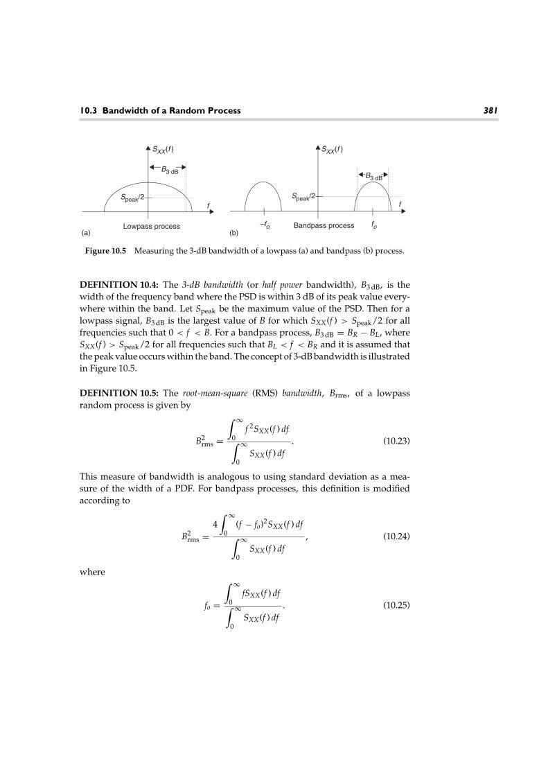
10.3 Bandwidth of a Random Process 381
f
Lowpass process(a) (b)
Bandpass process
Speak/2
SXX(f )
B3 dB
B3 dB
–fo
Speak/2
SXX(f )
fo
f
Figure 10.5 Measuring the 3-dB bandwidth of a lowpass (a) and bandpass (b) process.
DEFINITION 10.4: The 3-dB bandwidth (or half power bandwidth), B3 dB, is thewidth of the frequency band where the PSD is within 3 dB of its peak value every-where within the band. Let Speak be the maximum value of the PSD. Then for alowpass signal, B3 dB is the largest value of B for which SXX(f ) > Speak/2 for allfrequencies such that 0 < f < B. For a bandpass process, B3 dB = BR − BL, whereSXX(f ) > Speak/2 for all frequencies such that BL < f < BR and it is assumed thatthe peak value occurs within the band. The concept of 3-dB bandwidth is illustratedin Figure 10.5.
DEFINITION 10.5: The root-mean-square (RMS) bandwidth, Brms, of a lowpassrandom process is given by
B2rms =
∫ ∞
0f 2SXX(f ) df
∫ ∞
0SXX(f ) df
. (10.23)
This measure of bandwidth is analogous to using standard deviation as a mea-sure of the width of a PDF. For bandpass processes, this definition is modifiedaccording to
B2rms =
4∫ ∞
0(f − fo)2SXX(f ) df∫ ∞
0SXX(f ) df
, (10.24)
where
fo =
∫ ∞
0fSXX(f ) df
∫ ∞
0SXX(f ) df
. (10.25)

382 Chapter 10 Power Spectral Density
It is left as an exercise for the reader to figure out why the factor of 4 appears in thepreceding definition.
EXAMPLE 10.6: Consider the random telegraph process of Example10.4 where the PSD was found to be
SXX(f ) = λ
λ2 + (π f )2 .
The absolute bandwidth of this process is Babs = ∞. This can be seenfrom the picture of the PSD in Figure 10.2. To find the 3-dB bandwidth,it is noted that the peak of the PSD occurs at f = 0 and has a valueof Speak = λ−1. The 3-dB bandwidth is then the value of f for whichSXX(f ) = 1/(2λ). This is easily found to be B3 dB = λ/π . Finally, theRMS bandwidth of this process is infinite since
∫ ∞
0
λf 2
λ2 + (π f )2 df = ∞.
10.4 Spectral Estimation
The problem of estimating the PSD of a random process has been the topic of exten-sive research over the past several decades. Many books are dedicated to this topicalone and hence we cannot hope to give a complete treatment of the subject here;however, some fundamental concepts are introduced in this section that will pro-vide the reader with a basic understanding of the problem and some rudimentarysolutions. Spectral estimators are generally grouped into two classes, parametricand nonparametric. A parametric estimator assumes a certain model for the ran-dom process with several unknown parameters and then attempts to estimate theparameters. Given the model parameters, the PSD is then computed analyticallyfrom the model. On the other hand, a nonparametric estimator makes no assump-tions about the nature of the random process and estimates the PSD directly. Sinceparametric estimators take advantage of some prior knowledge of the nature of theprocess, it would be expected that these estimators are more accurate. However, insome cases, prior knowledge may not be available, in which case a nonparametric

10.4 Spectral Estimation 383
estimator may be more appropriate. We start with a description of some basictechniques for nonparametric spectral estimation.
10.4.1 Nonparametric Spectral Estimation
Suppose we observe a random process, X(t), over some time interval (−to, to) (ora discrete time process X[n] over some time interval [0, no − 1]) and we wishto estimate its PSD function. Two approaches immediately come to mind. Thefirst method we will refer to as the direct method, or the periodogram. It is basedon the definition of PSD in Equation 10.11. The second method we will refer toas the indirect method, or the correlation method. The basic idea here is to estimatethe autocorrelation function and then take the Fourier transform of the estimatedautocorrelation to form an estimate of the PSD. We first describe the correlationmethod. In all of the discussion on spectral estimation to follow, it is assumed thatthe random processes are WSS.
An estimate of the autocorrelation function of a continuous time randomprocess can be formed by taking a time average of the particular realizationobserved:
RXX(τ ) =⟨X(
t − τ
2
)X(
t + τ
2
)⟩= 1
2to − |τ |∫ to−|τ |
2
to+|τ |2
X(
t − τ
2
)X(
t + τ
2
)dt.
(10.26)
It is not difficult to show that this estimator is unbiased (i.e., E[RXX(τ )] = RXX(τ )),but at times it is not a particularly good estimator, especially for large values of τ .The next example illustrates this fact.
EXAMPLE 10.7: Consider the random telegraph process of Example10.4. A sample realization of this process is shown in Figure 10.6, alongwith the estimate of the autocorrelation function. For convenience, thetrue autocorrelation is shown as well. Note that the estimate matchesquite well for small values of τ , but as |τ | → to, the estimate becomesvery bad.
In order to improve the quality of the autocorrelation estimate, it is commonto introduce a windowing function to suppress the erratic behavior of the esti-mate at large values of τ . This is particularly important when estimating the PSDbecause the wild behavior at large values of |τ | will distort the estimate of the

384 Chapter 10 Power Spectral Density
0 5 10 15 20 25−1
−0.5
0
0.5
1
Time, t
X(t
)
−25 −20 −15 −10 −5 0 5 10 15 20 25 −1
−0.5
0
0.5
1
τ
Est
imat
e of
RX
X(τ
)
(a)
(b)
Figure 10.6 A sample realization of the random telegraph signal (a) and the estimateof the autocorrelation function based on that realization (b). The dotted line is the trueautocorrelation function.
PSD at all frequencies once the Fourier transform of the autocorrelation estimate istaken.
DEFINITION 10.6: For a WSS random process X(t), the windowed estimate of theautocorrelation function using a windowing function w(t) is given by
R (w)XX (τ ) = w(τ )
2to − |τ |∫ to−|τ |
2
to+|τ |2
X(
t − τ
2
)X(
t + τ
2
)dt. (10.27)
There are many possible windowing functions that can be used. The previousautocorrelation estimate (without the windowing function) can be viewed as awindowed estimate with a rectangular window,
w(t) = rect(
t4to
). (10.28)
Another option would be to use a triangular window,
w(t) = tri(
t2to
)=
1 − |t|2to
|t| < to
0 |t| > to
. (10.29)
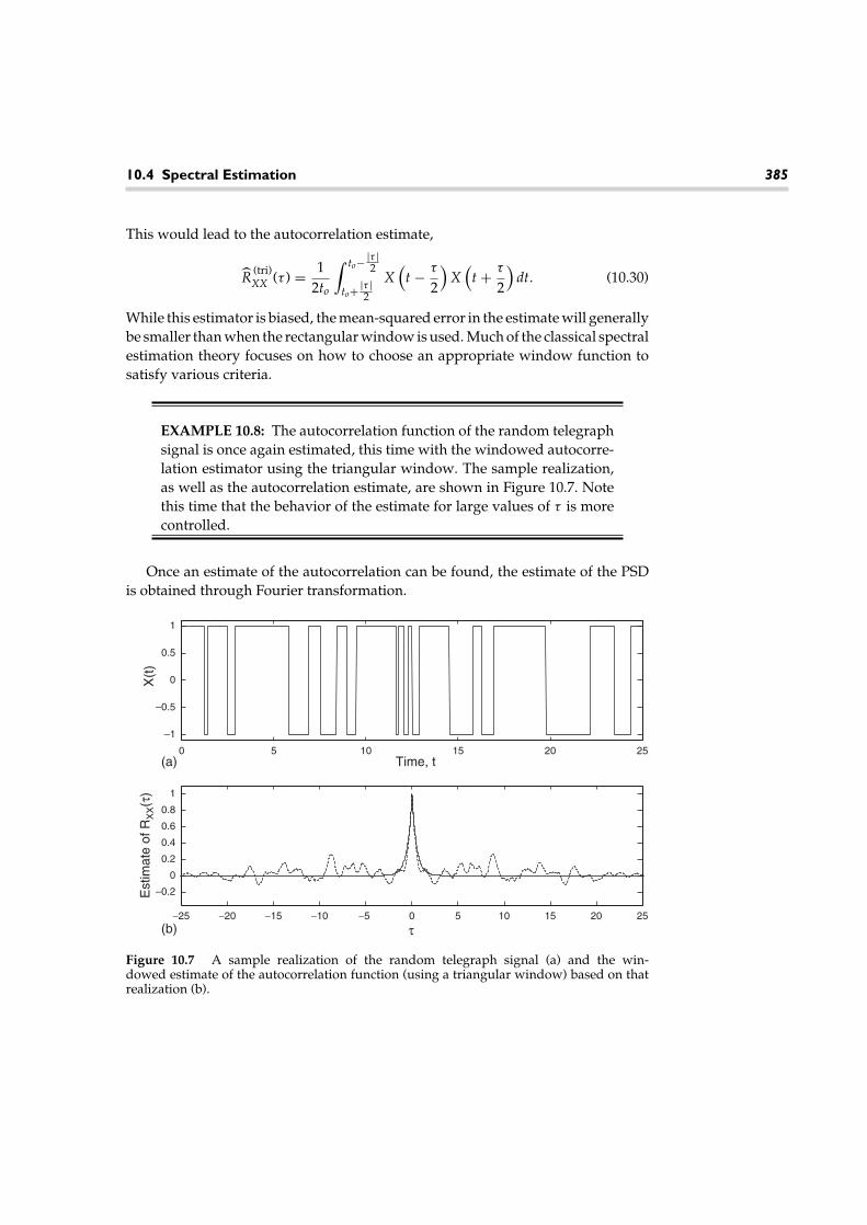
10.4 Spectral Estimation 385
This would lead to the autocorrelation estimate,
R (tri)XX (τ ) = 1
2to
∫ to−|τ |2
to+|τ |2
X(
t − τ
2
)X(
t + τ
2
)dt. (10.30)
While this estimator is biased, the mean-squared error in the estimate will generallybe smaller than when the rectangular window is used. Much of the classical spectralestimation theory focuses on how to choose an appropriate window function tosatisfy various criteria.
EXAMPLE 10.8: The autocorrelation function of the random telegraphsignal is once again estimated, this time with the windowed autocorre-lation estimator using the triangular window. The sample realization,as well as the autocorrelation estimate, are shown in Figure 10.7. Notethis time that the behavior of the estimate for large values of τ is morecontrolled.
Once an estimate of the autocorrelation can be found, the estimate of the PSDis obtained through Fourier transformation.
0 5 10 15 20 25
–1
–0.5
0
0.5
1
Time, t(a)
(b)
X(t
)
−25 −20 −15 −10 −5 0 5 10 15 20 25
–0.2
0
0.2
0.4
0.6
0.8
1
τ
Est
imat
e of
RX
X(τ
)
Figure 10.7 A sample realization of the random telegraph signal (a) and the win-dowed estimate of the autocorrelation function (using a triangular window) based on thatrealization (b).

386 Chapter 10 Power Spectral Density
DEFINITION 10.7: For a WSS random process X(t), the correlation-based estimate(with windowing function w(t)) of the PSD is given by
S (w)XX (f ) = F
[R (w)
XX (τ )]
=∫ ∞
−∞R (w)
XX (τ )e−j2π f τ dτ =∫ 2to
−2to
R (w)XX (τ )e−j2π f τ dτ . (10.31)
EXAMPLE 10.9: The PSD estimates corresponding to the autocorrela-tion estimates of the previous example are illustrated in Figure 10.8.There the correlation based PSD estimates are plotted and comparedwith the true PSD. Note that when no windowing is used, the PSD esti-mate tends to overestimate the true PSD. Another observation is that itappears from these results that the PSD estimates could be improvedby smoothing. We will elaborate on that shortly.
0 1 2 3 4 5 6 7 8 –1
–0.5
0
0.5
1
Time (seconds)
X(t
)
–40
–30
–20
–10
0
PS
D (
dB)
–40 –30 –20 –10 0 10 20 30 40
–40
–30
–20
–10
0
Frequency (Hz)
–40 –30 –20 –10 0 10 20 30 40
Frequency (Hz)
PS
D (
dB)
(a)
(b)
(c)
Figure 10.8 A sample realization of the random telegraph signal (a) and the estimate ofthe PSD function (b, c). Plot (b) is for the unwindowed estimator, while plot (c) is for thetriangular windowed estimator. For both PSD plots, the smooth thick line is the true PSD.

10.4 Spectral Estimation 387
The next approach we consider for estimating the PSD of a random process isto directly use the definition of PSD in Equation 10.11. This approach is referred toas the periodogram estimate.
DEFINITION 10.8: Given an observation of the process X(t) over an interval(−to, to), Xto (t), the periodogram estimate of the PSD is
S (p)XX(f ) = 1
2to
∣∣Xto (f )∣∣2 . (10.32)
THEOREM 10.2: The periodogram estimate of the PSD is equivalent to theautocorrelation-based estimate with a triangular window. That is,
S (p)XX(f ) = S (tri)
XX (f ). (10.33)
PROOF: The proof of this theorem is a fairly elementary exercise in manipulatingthe properties of Fourier transforms. Recall that for any two signals, x(t) and y(t),the product of their spectra forms a transform pair with the convolution of the twosignals. That is, F[x(t) ∗ y(t)] = X(f )Y(f ). Applying this to Equation 10.32 results in
∣∣Xto (f )∣∣2 = F [Xto (τ ) ∗ Xto (−τ )] = F
[∫ ∞
−∞Xto (u)Xto (u − τ ) du
]
= F[∫ to
−to
Xto (t)Xto (t + τ ) dt]
,
12to
∣∣Xto (f )∣∣2 = F
[1
2to
∫ to
−to
Xto (t)Xto (t + τ ) dt]
= F[R (tri)
XX (τ )]
= S (tri)XX (f ). (10.34)
�
An example of the periodogram was given in plot (c) of Figure 10.8. At the time,it was referred to as the correlation-based estimate with a triangular windowingfunction. Now it is clear that the two are the same. It was mentioned in Example 10.9that the quality of the periodogram might be improved by smoothing the PSD
estimate. This can be accomplished by convolving S (p)XX(f ) with some smoothing
function, w(f ).
DEFINITION 10.9: The smoothed periodogram with smoothing function w(f ) isgiven by
S (wp)XX (f ) = w(f ) ∗ S (p)
XX(f ). (10.35)

388 Chapter 10 Power Spectral Density
The smoothed periodogram can be viewed in terms of the correlation-basedestimate as well. Note that if w(τ ) = F−1[w(f )], then
S (wp)XX (f ) = F[w(τ )] ∗ F[R (tri)
XX (τ )] = F[w(τ )R (tri)XX (τ )]. (10.36)
Hence, the smoothed periodogram is nothing more than the windowed correlation-based estimate with a window that is the product of w(t) and the triangular window.This seems to indicate that there would be some potential benefit to using window-ing functions other than what has been presented here. The reader is referred tothe many books on spectral estimation in the literature for discussions of otherpossibilities.
In all of the spectral estimators presented thus far, an ensemble average wasestimated using a single realization. A better estimate could be obtained if sev-eral independent realizations of the random process were observed and a sampleaverage were used to replace the ensemble average. Even though we may be ableto observe only a single realization, it may still be possible to achieve the sameeffect. This is done by breaking the observed time waveform into segments andtreating each segment as an independent realization of the random process. Theperiodogram is computed on each segment and then the resulting estimates areaveraged.
EXAMPLE 10.10: Figure 10.9 compares the periodogram estimateof the PSD of the random telegraph signal with and without seg-mentation. In plot (b) no segmentation is used, while in plot (c) thedata is segmented into M = 8 frames. A periodogram is computed
for each frame and the results are then averaged. Note the improvement in thePSD estimate when the segmentation is used. Also note that there is a slightbias appearing in the segmented estimate. This is most noticeable at the higherfrequencies. This bias will get worse as more segments are used. There is atrade-off in wanting to use a large value of M to reduce the “jitter” in the esti-mate and wanting to use a small value of M to keep the bias to a minimum.The following MATLAB functions were used to implement the periodogramestimates with and without seqmentation. These same functions can be usedto estimate the PSD of any input signal.
function [Shat, f]=Periodogram(x,dx)
% This function computes the periodogram estimate of the PSD
% of the input signal. The vector x contains the samples of the
% input while dx indicates the time interval between samples.
Nx=length(x);

10.4 Spectral Estimation 389
0 1 2 3 4 5 6 7 8 9 –1
–0.5
0
0.5
1
Time (seconds)
X(t
)
–40 –30 –20 –10 0 10 20 30 40
–40
–30
–20
–10
0
Frequency (Hz)
PS
D (
dB)
–40 –30 –20 –10 0 10 20 30 40
–40
–30
–20
–10
Frequency (Hz)
PS
D (
dB)
(a)
(b)
(c)
Figure 10.9 A sample realization of the random telegraph signal (a) and the periodogramestimate of the PSD function (b, c). Plot (b) is for the unsegmented data, while plot (c) is forwhen the data is segmented into M = 8 frames. For both PSD plots, the smooth thick line isthe true PSD.
Rhat=conv(x,fliplr(x))/Nx;
Nr=length(Rhat);
Shat=fft(Rhat);
Shat=fftshift(dx*abs(Shat));
Nf=(Nr-1)/2; df=1/(dx*Nr);
f=[-Nf:Nf]*df;
function [S,f]=EPrdgm(x,dx,M)
% This function computes the periodogram estimate of the PSD
% of the input signal by breaking the signal into M frames and
% and performing a periodogram estimate on each frame and then
% averaging the results. The vector x contains the samples of
% the signal, while dx is the sampling interval. S is the
% estimated PSD and f is a vector of frequency samples that
% gives the frequency scale to be used when plotting S.

390 Chapter 10 Power Spectral Density
Nx=length(x);
Nframe=floor(Nx/M); % frame length
S=zeros(1,2*Nframe-1);
for m=1:M
xm=x(((m-1)*Nframe+1):(m*Nframe));
[Stemp,f]=Periodogram(xm,dx);
S=S+Stemp;
end
S=S/M;
10.4.2 Parametric Spectral Estimation
In parametric spectral estimation, a general model of the data is assumed, whichusually contains one or more unknown parameters. Given the general model, thePSD can be calculated analytically. The problem then becomes one of estimatingthe unknown parameters and plugging the result into the analytic form of the PSD.To provide an example of how this general approach works, we present a specificclass of random process models.
DEFINITION 10.10: Given a process X[n] with known statistics, a new process,Y[n], is formed according to the difference equation:
a0Y[n] =p∑
i=1
aiY[n − i] +q∑
i=0
biX[n − i]. (10.37)
This process is referred to as an autoregressive moving average process (ARMA). Asspecial cases, if all of the ai are equal to zero (except a0, which is usually set equalto unity), then Equation 10.37 simplifies to
Y[n] =q∑
i=0
biX[n − i], (10.38)
and the process is referred to as a moving average (MA) process. The notation MA(q)is used to refer to a qth order moving average process. If all of the bi are equal tozero except for b0, then the difference equation becomes
a0Y[n] =p∑
i=0
aiY[n − i] + b0X[n], (10.39)

10.4 Spectral Estimation 391
and the process is referred to as an autoregressive (AR) process. The notation AR(p)is used to refer to a pth order autoregressive process. For the general case, thenotation ARMA(p, q) is used.
To demonstrate the basic principles of parametric estimation, suppose it wasdetermined that a certain random process, Y[n], is well modeled by an AR(1) model,
Y[n] = a1Y[n − 1] + X[n], (10.40)
where X[n] is a IID random process with zero-mean and a variance of σ 2X . It is noted
that
Y[n + 1] = a1Y[n] + X[n + 1], (10.41)
Y[n + 2] = a21Y[n] + a1X[n + 1] + X[n + 2], (10.42)
Y[n + 3] = a31Y[n] + a2
1X[n] + a1X[n + 1] + X[n + 2], (10.43)
and in general,
Y[n + k] = ak1Y[n] +
k−1∑i=0
ak−1−i1 X[n + i]. (10.44)
Using this expression, the autocorrelation function of the AR(1) process can becomputed.
RYY[n, n + k] = E[Y[n]Y[n + k]]
= ak1E[Y2[n]] +
k−1∑i=0
ak−1−i1 E[Y[n]X[n + i]] = ak
1RYY[n, n] (10.45)
The last step is accomplished using the fact that Y[n] is independent of X[n + i] fori > 0. The expression RYY[n, n] is calculated according to
RYY[n, n] = E[(a1Y[n − 1] + X[n])2] = a21RYY[n − 1, n − 1] + σ 2
X . (10.46)
Assuming that the process Y[n] is WSS3, this recursion becomes
RYY[0] = a21RYY[0] + σ 2
X ⇒ RYY[0] = σ 2X
1 − a21
. (10.47)
3It will be shown in the next chapter that this is the case provided that X[n] is WSS.

392 Chapter 10 Power Spectral Density
Hence, the autocorrelation function of the AR(1) process is
RYY[k] = σ 2X
1 − a21
a|k|1 . (10.48)
Assuming that the samples of this discrete time process are taken at a samplinginterval of t, the PSD of this process works out to be
SYY(f ) = tσ 2X∣∣1 − a1e−j2π f t
∣∣2 . (10.49)
For this simple AR(1) model, the PSD can be expressed as a function of twounknown parameters, a1 and σ 2
X . The problem of estimating the PSD then becomesone of estimating the two parameters and then plugging the result into the gen-eral expression for the PSD. In many cases, the total power in the process maybe known, which eliminates the need to estimate σ 2
X . Even if that is not the case,the value of σ 2
X is just a multiplicative factor in the expression for PSD and doesnot change the shape of the curve. Hence, in the following, we focus attention onestimating the parameter, a1.
Since we know the AR(1) model satisfies the recursion of Equation 10.40, thenext value of the process can be predicted from the current value according to
Y[n + 1] = a1Y[n]. (10.50)
This is known as linear prediction since the predictor of the next value is a linearfunction of the current value. The error in this estimate is
E = Y[n + 1] − Y[n + 1] − Y[n + 1] − a1Y[n]. (10.51)
Typically, we choose as an estimate of a1 the value of a1 that makes the linearpredictor as good as possible. Usually, “good” is interpreted as minimizing themean-square error, which is given by
E[E2] = E[(Y[n + 1] − a1Y[n])2] = RYY(0)(1 + a21) − 2a1RYY(1). (10.52)
Differentiating the mean-square error with respect to a1 and setting equal to zeroresults in
2a1RYY(0) − 2RYY(1) = 0 ⇒ a1 = RYY(1)RYY(0)
. (10.53)
Of course, we don’t know what the autocorrelation function is. If we did, wewould not need to estimate the PSD. So, the preceding ensemble averages must

10.4 Spectral Estimation 393
be replaced with sample averages, and the minimum mean-square error (MMSE)linear prediction coefficient is given by
a1 = RYY(1)
RYY(0)=∑n0−1
n=−n0y[n]y[n + 1]∑n0
n=−n0y2[n] . (10.54)
Note that we have used a lower case y[n] in Equation 10.54 since we are dealingwith a single realization rather than the ensemble Y[n].
EXAMPLE 10.11: In this example, we use the AR(1) model to estimatethe PSD of the random telegraph process. Clearly, the AR(1) model doesnot describe the random telegraph process; however, the autocorrela-tion function of the random telegraph signal is a two-sided exponential,as is the autocorrelation function of the AR(1) process. As a conse-quence, we expect this model to give good results. The results areshown in Figure 10.10. Notice how nicely the estimated PSD matchesthe actual PSD.
0 2 4 6 8 10 12 14 16–1
–0.5
0
0.5
1
Time (seconds)(a)
(b)
X(t
)
−40 −30 −20 −10 0 10 20 30 40
–40
–30
–20
–10
0
Frequency (Hz)
PS
D (
dB)
Estimated PSDActual PSD
Figure 10.10 A sample realization of the random telegraph signal (a) and the parametricestimate of the PSD function based on the AR(1) model (b).
394 Chapter 10 Power Spectral Density
In the previous example, the results were quite good because the functionalform of the PSD of the AR(1) process nicely matched the functional form of thetrue PSD. If the fit had not been so good, it might have been necessary to moveto a higher order AR(p) model. In the exercises at the end of the chapter (seeExercises 10.19 and 10.20), the reader is led through the problem of finding theMMSE linear prediction coefficients for a general AR(p) model. The problem ofanalytically finding the PSD of the AR(p) process is dealt with in the next chapter(also see Exercise 10.18).
10.5 Thermal Noise
The most commonly encountered source of noise in electronic systems is thatcaused by thermal agitation of electrons in any conductive material, which is com-monly referred to as thermal noise. Unlike shot noise, thermal noise does not requirethe presence of a direct current and thus is always present. We will not delve intothe underlying thermodynamics to derive a model for this type of noise, but ratherwill just summarize some of the important results. Nyquist’s theorem states thatfor a resistive element with an impedance of r ohms (), at a temperature of tk(measured in degrees Kelvin), the mean-square voltage of the thermal noise mea-sured in an incremental frequency band of width f centered at frequency f isfound to be
E[V2(t)] = v2rms = 4ktkrf
[h|f |/ktk
exp(h|f |/ktk) − 1
]volts2, (10.55)
where
h = Planck’s constant = 6. 2 × 10⁻³⁴ J-sec;k = Boltzman’s constant = 1. 38 × 10−23 J/◦K;tk = absolute temperature = 273 +◦C.
Typically, a practical resistor is modeled as a Thevenin equivalent circuit, asillustrated in Figure 10.11, consisting of a noiseless resistor in series with a noisesource with a mean-square value as specified in the previous equation. If this noisyresistor were connected to a resistive load of impedance rL, the average powerdelivered to the load would be
PL = v2rmsrL
(r + rL)2 . (10.56)
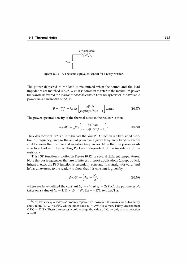
10.5 Thermal Noise 395
vrms ∼
r (noiseless)
Figure 10.11 A Thevenin equivalent circuit for a noisy resistor.
The power delivered to the load is maximized when the source and the loadimpedance are matched (i.e., rL = r). It is common to refer to the maximum powerthat can be delivered to a load as the available power. For a noisy resistor, the availablepower (in a bandwidth of f ) is
P = v2rms4r
= ktkf[
h|f |/ktk
exp(h|f |/ktk) − 1
]watts. (10.57)
The power spectral density of the thermal noise in the resistor is then
SNN(f ) = 12
ktk
[h|f |/ktk
exp(h|f |/ktk) − 1
]. (10.58)
The extra factor of 1/2 is due to the fact that our PSD function is a two-sided func-tion of frequency, and so the actual power in a given frequency band is evenlysplit between the positive and negative frequencies. Note that the power avail-able to a load and the resulting PSD are independent of the impedance of theresistor, r.
This PSD function is plotted in Figure 10.12 for several different temperatures.Note that for frequencies that are of interest in most applications (except optical,infrared, etc.), the PSD function is essentially constant. It is straightforward (andleft as an exercise to the reader) to show that this constant is given by
SNN(f ) = 12
ktk = No
2, (10.59)
where we have defined the constant No = ktf . At tk = 298◦K4, the parameter No
takes on a value of No = 4. 11 × 10−21 W/Hz = −173. 86 dBm/Hz.
4Most texts use tk = 290◦K as “room temperature”; however, this corresponds to a fairlychilly room (17◦C ≈ 63◦F ). On the other hand tk = 298◦K is a more balmy environment(25◦C ≈ 77◦F ). These differences would change the value of No by only a small fractionof a dB.

396 Chapter 10 Power Spectral Density
106 108 1010 1012 1014–210
–205
–200
–195
–190
–185
–180
–175
–170
Frequency (Hz)
PS
D (
dBm
/Hz)
tk = 300°K
tk = 30°K
tk = 3°Ktk = 3°K
Figure 10.12 PSD of thermal noise in a resistor.
It is common to use this simpler function as a model for the PSD of thermalnoise. Because the PSD contains equal power at all frequencies, this noise model isreferred to as white noise (analogous to white light, which contains all frequencies).The corresponding autocorrelation function is
RNN(τ ) = No
2δ(τ ). (10.60)
It should be pointed out that the noise model of Equation 10.59 is a mathematicalapproximation to the actual PSD. There is no such thing as truly white noise, sincesuch a process (if it existed) would have infinite power and would destroy anydevice we tried to measure it with. However, this mathematical model is simple,easy to work with, and serves as a good approximation to thermal noise for mostapplications.
In addition to modeling thermal noise as having a flat PSD, it can also be shownthat the first order characteristics of thermal noise can be well approximated witha zero-mean Gaussian process. We say that thermal noise is zero-mean whiteGaussian noise (WGN) with a (two-sided) PSD of No/2. While thermal noise isthe most common source of noise in electronic devices, there are other sourcesas well. Shot noise was discussed at the end of Chapter 8. In addition, one mayencounter flicker noise, which occurs primarily in active devices; burst or popcorn

10.6 Engineering Application: PSDs of Digital Modulation Formats 397
noise, which is found in integrated circuits and some discrete transistors; avalanchenoise, which is produced by avalanche breakdown in a p-n junction; as well as sev-eral other types of noise. For the purposes of this text, we will stick with the whiteGaussian model of thermal noise.
10.6 Engineering Application: PSDs ofDigital Modulation Formats
In this section, we evaluate the PSD of a class of signals that might be used ina digital communications system. Suppose we have a sequence of data symbols{Bk} that we wish to convey across some communication medium. We can use thedata symbols to determine the amplitude of a sequence of pulses that we wouldthen transmit across the medium (e.g., a twisted copper pair, or an optical fiber).This is known as pulse amplitude modulation (PAM). If the pulse amplitudes arerepresented by the sequence of random variables {. . . , A−2, A−1, A0, A1, A2, . . .} andthe basic pulse shape is given by the waveform p(t), then the transmitted signalmight be of the form
S(t) =∞∑
k=−∞Akp(t − kts − �), (10.61)
where ts is the symbol interval (that is, one pulse is launched every ts seconds)and � is a random delay, which we take to be uniformly distributed over [0, ts)and independent of the pulse amplitudes. The addition of the random delay in themodel makes the process S(t) WSS. This is not necessary and the result we willobtain would not change if we did not add this delay, but it does slightly simplifythe derivation.
If the data symbols are drawn from an alphabet of size 2n symbols, then eachsymbol can be represented by an n-bit word, and hence the data rate of the digitalcommunication system is r = n/ts bits/second. The random process S(t) used torepresent this data has a certain spectral content, and thus requires a communica-tions channel with a bandwidth adequate to carry that spectral content. It wouldbe interesting to see how the required bandwidth relates to the data rate. Towardthat end, we seek to determine the PSD of the PAM signal S(t). We will find thePSD by first computing the autocorrelation function of S(t) and then convertingthis to PSD via the Wiener-Khintchine-Einstein theorem.
398 Chapter 10 Power Spectral Density
Using the definition of autocorrelation, the autocorrelation function of the PAMsignal is given by
RSS(t,t+τ )=E[S(t)S(t+τ )]=E
∞∑
k=−∞
∞∑m=−∞
AkAmp(t−kts−�)(p(t+τ −mts−�))
=∞∑
k=−∞
∞∑m=−∞
E[AkAm]E[p(t−kts−�)p(t+τ −mts−�)]
= 1ts
∞∑k=−∞
∞∑m=−∞
E[AkAm]∫ ts
0p(t−kts−θ )p(t+τ −mts−θ )]dθ . (10.62)
To simplify notation, we define RAA[n] to be the autocorrelation function of thesequence of pulse amplitudes. Note that we are assuming the sequence is stationary(at least in the wide sense). Going through a simple change of variables (v =t − kts − θ ) then results in
RSS(t, t + τ ) = 1ts
∞∑k=−∞
∞∑m=−∞
RAA[m − k]∫ t−ks
t−(k+1)ts
p(v)p(v + τ − (m − k)ts) dv.
(10.63)
Finally, we go through one last change of variables (n = m − k) to produce
RSS(t, t + τ ) = 1ts
∞∑k=−∞
∞∑n=−∞
RAA[n]∫ t−ks
t−(k+1)ts
p(v)p(v + τ − nts) dv
= 1ts
∞∑n=−∞
RAA[n]∞∑
k=−∞
∫ t−kts
t−(k+1)ts
p(v)p(v + τ − nts) dv
= 1ts
∞∑n=−∞
RAA[n]∫ ∞
−∞p(v)p(v + τ − nts) dv. (10.64)
To aid in taking the Fourier transform of this expression, we note that the integralin this equation can be written as a convolution of p(t) with p(−t):
∫ ∞
−∞p(v)p(v + τ − nts) dv = p(t)∗p(−t)|t=τ−nts . (10.65)
Using the fact that convolution in the time domain becomes multiplication in thefrequency domain along with the time reversal and time shifting properties ofFourier transforms (see Appendix C, Review of Linear Time Invariant Systems),

10.6 Engineering Application: PSDs of Digital Modulation Formats 399
the transform of this convolution works out to be
F[∫ ∞
−∞p(v)p(v + τ − nts) dv
]= |p(f )|2e−j2πnfts , (10.66)
where P(f ) = F[p(t)] is the Fourier transform of the pulse shape used. With thisresult, the PSD of the PAM signal is found by taking the transform of Equation10.64, resulting in
SSS(f ) = |P(f )|2ts
∞∑n=−∞
RAA[n]e−j2πnfts . (10.67)
It is seen from the previous equation that the PSD of a PAM signal is the productof two terms, the first of which is the magnitude squared of the pulse shapesspectrum, while the second term is essentially the PSD of the discrete sequence ofamplitudes. As a result, we can control the spectral content of our PAM signal bycarefully designing a pulse shape with a compact spectrum and also by introducingmemory into the sequence of pulse amplitudes.
EXAMPLE 10.12: To start with, suppose the pulse amplitudes are anIID sequence of random variables that are equally likely to be +1 or −1.In that case, RAA[n] = δ[n] and the PSD of the sequence of amplitudes is
∞∑n=−∞
RAA[n]e−j2πnfts = 1.
In this case, SSS(f ) = |P(f )|2/ts and the spectral shape of the PAMsignal is completely determined by the spectral content of the pulseshape. Suppose we use as a pulse shape a square pulse of height a andwidth ts,
p(t) = arect(t/ts) ←→ P(f ) = atssinc(fts).
The PSD of the resulting PAM signal is then SSS(f ) = a2tssinc2f (ts).Note that the factor a2ts is the energy in each pulse sent, Ep. A sam-ple realization of this PAM process along with a plot of the PSD isgiven in Figure 10.13. Most of the power in the process is contained inthe main lobe, which has a bandwidth of 1/ts (equal to the data rate),but there is also a nontrivial amount of power in the sidelobes, whichdie off very slowly. The high-frequency content can be attributed tothe instantaneous jumps in the process. These frequency sidelobes can
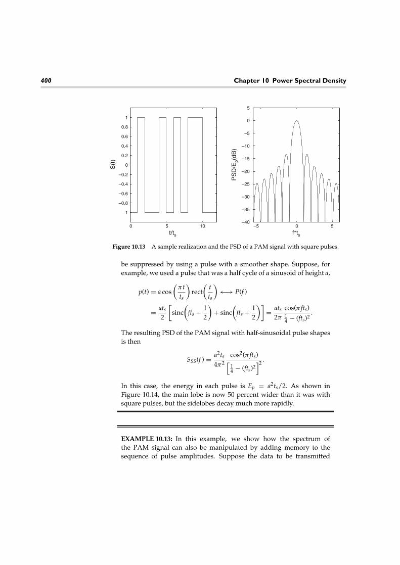
400 Chapter 10 Power Spectral Density
0 5 10
–1
–0.8
–0.6
–0.4
–0.2
0
0.2
0.4
0.6
0.8
1
t/ts
S(t
)
−5 0 5–40
–35
–30
–25
–20
–15
–10
–5
0
5
f*tsP
SD
/Ep(
dB)
Figure 10.13 A sample realization and the PSD of a PAM signal with square pulses.
be suppressed by using a pulse with a smoother shape. Suppose, forexample, we used a pulse that was a half cycle of a sinusoid of height a,
p(t) = a cos(
π tts
)rect
(tts
)←→ P(f )
= ats
2
[sinc
(fts − 1
2
)+ sinc
(fts + 1
2
)]= ats
2π
cos(π fts)14 − (fts)2
.
The resulting PSD of the PAM signal with half-sinusoidal pulse shapesis then
SSS(f ) = a2ts
4π2cos2(π fts)[14 − (fts)2
]2 .
In this case, the energy in each pulse is Ep = a2ts/2. As shown inFigure 10.14, the main lobe is now 50 percent wider than it was withsquare pulses, but the sidelobes decay much more rapidly.
EXAMPLE 10.13: In this example, we show how the spectrum ofthe PAM signal can also be manipulated by adding memory to thesequence of pulse amplitudes. Suppose the data to be transmitted

10.6 Engineering Application: PSDs of Digital Modulation Formats 401
0 5 10
−1
−0.8
−0.6
−0.4
−0.2
0
0.2
0.4
0.6
0.8
1
t/ts
S(t
)
−5 0 5−40
−35
−30
−25
−20
−15
−10
−5
0
5
f*ts
PS
D/E
p (d
B)
Figure 10.14 A sample realization and the PSD of a PAM signal with half-sinusoidal pulses.
{. . . , B−2, B−1, B0, B1, B2, . . .} is an IID sequence of Bernoulli random vari-ables, Bk ∈ {+1, −1}. In the previous example, we formed the pulseamplitudes according to Ak = Bk. Suppose instead that we formedthese amplitudes according to Ak = Bk + Bk−1. Now the pulse ampli-tudes can take on three values (even though each pulse still carries only1 bit of information. This is known as duobinary precoding. The resultingautocorrelation function for the sequence of pulse amplitudes is
RAA[n] = E[AkAk+n] = E[(Bk + Bk−1)(Bk+n + Bk+n−1] =
2 n = 0
1 n = ±1
0 otherwise
.
The PSD of this sequence of pulse amplitudes is then
∞∑n=−∞
RAA[n]e−j2π fts = 2 + ej2π fts + e−j2πnfts
= 2 + 2 cos(2π fts) = 4 cos2(π fts).
This expression then multiplies whatever spectral shape results fromthe pulse shape chosen. The PSD of duobinary PAM with square pulses

402 Chapter 10 Power Spectral Density
0 5 10
–2
–1.5
–1
–0.5
0
0.5
1
1.5
2
t/ts
S(t
)
–5 0 5–40
–35
–30
–25
–20
–15
–10
–5
0
5
f*ts
PS
D/E
p (d
B)
Figure 10.15 A sample realization and the PSD of a PAM signal with duobinary precodingand square pulses.
is illustrated in Figure 10.15. In this case, the duobinary precoding hasthe benefit of suppressing the frequency sidelobes without broadeningthe main lobe.
EXAMPLE 10.14: The following MATLAB code creates a realiza-tion of a binary PAM signal where the pulse amplitudes are either+1 or −1. In this example, a half-sinusoidal pulse shape is used,but the code is written so that it is easy to change the pulse shape
(just change the sixth line where the pulse shape is assigned to the variable p).After a realization of the PAM signal is created, the PSD of the resulting signalis estimated using the segmented periodogram technique given in Example10.10. The resulting PSD estimate is shown in Figure 10.16. Note the agree-ment between the estimate and the actual PSD shown in Figure 10.14. Thereader is encouraged to try running this program with different pulse shapesto see how the pulse shape changes the spectrum of the PAM signal.

10.6 Engineering Application: PSDs of Digital Modulation Formats 403
–40 –30 –20 –10 0 10 20 30 40–60
–50
–40
–30
–20
–10
0
10
Frequency (kHz)
PS
D (
dB)
Figure 10.16 An estimate of the PSD of a PAM signal with half-sinusoidal pulse shapes.
N=100; % Number of bit intervals in
realization.
Ns=19; % Number of time samples per bit.
Rb=9600; % Bit rate (bits/sec).
dt=1/(Rb*Ns); % Time between samples.
t=([1:Ns]-0.5)/Ns; % Time axis for pulse shape.
p=sin(pi*t); % Pulse shape.
Ep=p*p’*dt; % Energy per pulse.
X(1:Ns:(Ns*(N-1)+1)) % Random data bits.
=sign(rand(1,N)-0.5);
X=conv(X,p); % PAM signal with pulse shape
added.
M=10; % Number of segments.
[S,f]=EPrdgm(X,dt,M); % (Normalized) PSD estimate.
plot(f/1000,10*log10(abs(S/Ep))) % Plot results.
axis([-5*Rb/1000 5*Rb/1000 -60 10])
xlabel(‘frequency (kHz)’)
ylabel(‘PSD (dB)’)

404 Chapter 10 Power Spectral Density
Exercises10.1 Consider a random process of the form
X(t) = b cos(2π�t + �),
where b is a constant, � is a uniform random variable over [0, 2π ), and �
is a random variable that is independent of � and has a PDF, f� (ψ). Findthe PSD, SXX(f ) in terms of f� (ψ). In so doing, prove that for any S(f ) thatis a valid PSD function, we can always construct a random process withPSD equal to S(f ).
10.2 Let X(t) = A cos(ωt) + B sin(ωt) where A and B are independent, zero-mean, identically distributed non-Gaussian random variables (IID). Showthat X(t) is wide sense stationary (WSS), but not strict sense stationary.Hint: For the latter case, consider E[X3(t)]. Recall the discussion prior toExample 8.23. If A and B are Gaussian, with zero mean and (IID), then X(t)is strict sense stationary.
10.3 Let X(t) = ∑Nn=1 an cos(ωnt+θn), where all of the ωn are nonzero constants,
the an are constants, and the θn are IID random variables, each uniformlydistributed over [0, 2π ).
(a) Determine the autocorrelation function of X(t).(b) Determine the power spectral density of X(t).
10.4 Let X(t) = ∑∞n=1[An cos(nωt) + Bn sin(nωt)] be a random process, where
An and Bn are random variables such that E[An] = E[Bn] = 0, E[AnBm] = 0,E[AnAm] = δn,mE
[A2
n], and E[BnBm] = δn,mE
[B2
n]
for all m and n, where δn,m
is the Kronecker delta function. This process is sometimes used as a modelfor random noise.
(a) Find the time-varying autocorrelation function RXX(t, t + τ ).(b) If E
[B2
n] = E
[A2
n], is this process WSS?
10.5 Find the power spectral density for a process for which RXX(τ ) = 1for all τ .
10.6 Suppose X(t) is a stationary, zero-mean Gaussian random process withPSD, SXX(f ).
(a) Find the PSD of Y(t) = X2(t) in terms of SXX(f ).
(b) Sketch the resulting PSD if SXX(f ) = rect(
f2B
).
(c) Is Y(t) WSS?

Exercises 405
10.7 Consider a random sinusoidal process of the form X(t) = b cos(2π ft + �),where � has an arbitrary PDF, f�(θ ). Determine analytically how the PSDof X(t) depends on f�(θ ). Give an intuitive explanation for your result.
10.8 Let s(t) be a deterministic periodic waveform with period to. A randomprocess is constructed according to X(t) = s(t − T), where T is a randomvariable uniformly distributed over [0, to). Show that the random processX(t) has a line spectrum and write the PSD of X(t) in terms of the FourierSeries coefficients of the periodic signal s(t).
10.9 A sinusoidal signal of the form X(t) = b cos(2π fot +�) is transmitted froma fixed platform. The signal is received by an antenna on a mobile platformthat is in motion relative to the transmitter, with a velocity of V relative tothe direction of signal propagation between the transmitter and receiver.Hence, the received signal experiences a Doppler shift and (ignoring noisein the receiver) is of the form.
Y(t) = b cos(
2π fo
(1 + V
c
)t + �
),
where c is the speed of light. Find the PSD of the received signal if V isuniformly distributed over (−vo, vo). Qualitatively, what does the Dopplereffect do to the PSD of the sinusoidal signal?
10.10 Two zero-mean, discrete random processes, X[n] and Y[n], are statisticallyindependent and have autocorrelation functions given by RXX[k] = (1/2)k
and RYY[k] = (1/3)k. Let a new random process be Z[n] = X[n] + Y[n].(a) Find RZZ[k]. Plot all three autocorrelation functions.(b) Determine all three power spectral density functions analytically and
plot the power spectral densities.
10.11 Let SXX(f ) be the PSD function of a WSS discrete time process X[n].Recall that one way to obtain this PSD function is to compute RXX[n] =E[X[k]X[k+n]] and then take the DFT of the resulting autocorrelation func-tion. Determine how to find the average power in a discrete time randomprocess directly from the PSD function, SXX(f ).
10.12 A binary phase shift keying signal is defined according to
X(t) = cos(
2π fct + B[n]π2
)for nT ≤ t < (n + 1)T,
for all n, and B[n] is a discrete time, Bernoulli random process that hasvalues of +1 or −1.

406 Chapter 10 Power Spectral Density
(a) Determine the autocorrelation function for the random process X(t).Is the process WSS?
(b) Determine the power spectral density of X(t).
10.13 Develop a formula to compute the RMS bandwidth of a random process,X(t), directly from its autocorrelation function, RXX(τ ).
10.14 A random process has a PSD function given by
S(f ) = 1(1 +
(fB
)2)3 .
(a) Find the absolute bandwidth.(b) Find the 3-dB bandwidth.(c) Find the RMS bandwidth.
Can you generalize your result to a spectrum of the form
S(f ) = 1(1 +
(fB
)2)N ,
where N is an integer greater than 1?
10.15 A random process has a PSD function given by
S(f ) = f 2
(1 +
(fB
)2)3 .
(a) Find the absolute bandwidth.(b) Find the 3-dB bandwidth.(c) Find the RMS bandwidth.
Can you generalize your result to a spectrum of the form
S(f ) = f 2
(1 +
(fB
)2)N ,
where N is an integer greater than 2?

Exercises 407
10.16 Let X(t) be a random process whose PSD is shown in the accompanyingfigure. A new process is formed by multiplying X(t) by a carrier to produce
Y(t) = X(t) cos(ωot + �),
where � is uniform over [0, 2π ) and independent of X(t). Find and sketchthe PSD of the process Y(t).
f
SXX(f)
fo fo + B
1
10.17 Consider the linear prediction random process X[n] = (1/2)X[n−1]+E[n],n = 1, 2, 3, . . ., where X[0] = 0 and E[n] is a zero-mean, IID random process.Find the mean and autocorrelation functions for X[n]. Is X[n] WSS?
10.18 Consider an AR(2) process described by the recursion
Y[n] = a1Y[n − 1] + a2Y[n − 2] + X[n],where X[n] is an IID random process with zero-mean and variance σ 2
X .
(a) Show that the autocorrelation function of the AR(2) process satisfiesthe difference equation,
RYY[k] = a1RYY[k − 1] + a2RYY[k − 2], k = 2, 3, 4, . . . .
(b) Show that the first two terms in the autocorrelation function satisfy
(1 − a21 − a2
2)RYY[0] − 2a1a2RYY[1] = σ 2X ,
and
(1 − a2)RYY[1] = a1RYY[0].From these two equations, solve for RYY[0] and RYY[1] in terms of a1,a2, and σ 2
X .(c) Using the difference equation in part (a) together with the initial con-
ditions in part (b), find a general expression for the autocorrelationfunction of an AR(2) process.
(d) Use your result in part (c) to find the PSD of an AR(2) process.

408 Chapter 10 Power Spectral Density
10.19 Suppose we use an AR(2) model to predict the next value of a randomprocess based on observations of the two most recent samples. That is,we form
Y[n + 1] = a1Y[n] + a2Y[n − 1].(a) Derive an expression for the mean-square estimation error,
E[ε2] = E[(Y[n + 1] − Y[n + 1])2].
(b) Find the values of the prediction coefficients, a1 and a2, that minimizethe mean-square error.
10.20 Extend the results of Exercise 10.19 to a general AR(p) model. That is,suppose we wish to predict the next value of a random process by forminga linear combination of the p most recent samples:
Y[n + 1] =p∑
k=1
akY[n − k + 1].
Find an expression for the values of the prediction coefficients thatminimize the mean-square prediction error.
10.21 A random process Y[n] is found to obey the AR(2) model. That is, Y[n] =a1Y[n − 1] + a2Y[n − 2] + X[n]. Find expressions for the autocorrelationfunction and PSD of Y[n]. Can you generalize your results to an arbitraryAR(p) model?
10.22
(a) Prove that the expression for the PSD of thermal noise in a resistorconverges to the constant No/2 = ktk/2 as f → 0.
(b) Assuming a temperature of 298◦K, find the range of frequencies overwhich thermal noise has a PSD that is within 99 percent of its valueat f = 0.
(c) Suppose we had a very sensitive piece of equipment that was ableto accurately measure the thermal noise across a resistive element.Furthermore, suppose our equipment could respond to a range of fre-quencies that spanned 50 MHz. Find the power (in watts) and the rootmean square (RMS) voltage (in volts) that we would measure across a75 resistor. Assume the equipment had a load impedance matchedto the resistor.

MATLAB Exercises 409
10.23 Suppose two resistors of impedance r1 and r2 are placed in series and heldat different physical temperatures, t1 and t2. We would like to model thisseries combination of noisy resistors as a single noiseless resistor, with animpedance of r = r1 + r2, together with a noise source with an effectivetemperature of te. In short, we want the two models shown in the accom-panying figure to be equivalent. Assuming the noise produced by the tworesistors is independent, what should te, the effective noise temperature,of the series combination of resistors be? If the two resistors are held at thesame physical temperature, is the effective temperature equal to the truecommon temperature of the resistors?
~
~
~
vrms,1 = 4kt1r1∆f
r1 (noiseless)
r = r1 + r2 (noiseless)
r2 (noiseless)
vrms,2 = 4kt2r2∆f
vrms = 4kter∆f
10.24 Repeat Exercise 10.26 for a parallel combination of resistors.
MATLAB Exercises10.25
(a) Create a random process X[n] where each sample of the random pro-cess is an IID, Bernoulli random variable equally likely to be ±1. Forma new process according to the MA(2) model Y[n] = X[n]− 1
2 X[n−1]+14 X[n − 2]. Assume X[n] = 0 for n < 0.
(b) Compute the time average autocorrelation function 〈Y[n]Y[n+k]〉 froma single realization of this process.

410 Chapter 10 Power Spectral Density
(c) Compute the ensemble average autocorrelation function E[Y[n]Y ×[n + k]] from several realizations of this process. Does the processappear to be ergodic in the autocorrelation?
(d) Estimate the PSD of this process using the periodogram method.
10.26
(a) Create a random process X[n] where each sample of the random pro-cess is an IID, Bernoulli random variable equally likely to be ±1. Forma new process according to the AR(2) model Y[n] = 1
2 Y[n − 1] − 14 Y ×
[n − 2] + X[n]. Assume Y[n] = 0 for n < 0.(b) Compute the time average autocorrelation function 〈Y[n]Y[n+k]〉 from
a single realization of this process.(c) Compute the ensemble average autocorrelation function E[Y[n]Y ×
[n+k]] from several realizations of this process. Does the process appearto be ergodic in the autocorrelation?
(d) Estimate the PSD of this process using the periodogram method.
10.27
(a) For the process in Exercise 10.29, find a parametric estimate of the PSDby using an AR(1) model. Compare the resulting PSD estimate withthe nonparametric estimate found in Exercise 10.29(d). Explain anydifferences you see.
(b) Again referring to the process in Exercise 10.29, find a parametricestimate of the PSD this time by using an AR(2) model. Comparethe resulting PSD estimate with the nonparametric estimate found inExercise 10.29(d). Explain any differences you see.
10.28
(a) Write a MATLAB program to create a realization of a binary PAMsignal with square pulses. You can accomplish this with a simplemodification to the program as given in Example 10.14. Call thissignal x(t).
(b) We can create a frequency shift keying (FSK) signal according to
y(t) cos(
2π fct + π
2ts
∫ t
0x(u) du
), (10.68)
where ts is the duration of the square pulses in x(t) and fc is the carrierfrequency. Write a MATLAB program to create a 10-msec realizationof this FSK signal assuming ts = 100 µ sec and fc = 20 kHz.

MATLAB Exercises 411
(c) Using the segmented periodogram, estimate the PSD of the FSK signalyou created in part (b).
(d) Estimate the 30-dB bandwidth of the FSK signal. That is, find thebandwidth where the PSD is down 30 dB from its peak value.
10.29 Construct a signal-plus-noise random sequence using 10 samples of
X[n] = cos(2πnf0ts) + N[n],where N[n] is a sequence of zero-mean, unit variance, IID Gaussian ran-dom variables, f0 = 0. 1/ts = 100 kHz, and ts = 1 µsec is the time betweensamples of the process.
(a) Calculate the periodogram estimate of the PSD, SXX(f ).(b) Calculate a parametric estimate of the PSD using AR models with p =
1, 2, 3, and 5. Compare the parametric estimates with the periodogram.In your opinion, which order AR model is the best fit?
(c) Repeat parts (a) and (b) using 100 samples instead of 10.
10.30 Construct a signal-plus-noise random sequence using 10 samples of
X[n] = cos(2πnf1ts) + cos(2πnf2ts) + N[n],where N[n] is a sequence of zero-mean, unit variance, IID Gaussianrandom variables, f1 = 0. 1/ts = 100 kHz, f1 = 0. 4/ts = 400 kHz, andts = 1 µsec is the time between samples of the process.
(a) Calculate the periodogram estimate of the PSD, SXX(f ).(b) Calculate a parametric estimate of the PSD using AR models with
p = 3, 4, 5, 6, and 7. Compare the parametric estimates with theperiodogram. In your opinion, which order AR model is the best fit?
(c) Repeat parts (a) and (b) using 100 samples instead of 10.

Random Processesin Linear Systems 11
In this chapter, we consider the response of both continuous and discrete linearsystems to random processes, such as a signal plus noise. We develop statisticaldescriptions of the output of linear systems with random inputs by viewing thesystems in both the time domain and the frequency domain. Two engineeringapplication sections at the end of this chapter demonstrate how filters can be opti-mized for the purpose of enhancing signal-to-noise ratio and also for the purposeof prediction or smoothing of a signal in noise. It is assumed that the reader isfamiliar with the study of linear time invariant (LTI) systems. A brief overviewis provided in Appendix C, Review of Linear Time–Invariant Systems, for thoseneeding a refresher.
11.1 Continuous Time Linear Systems
Consider an LTI system described by an impulse response h(t) or a transfer functionH(f ). If a random process, X(t), is input to this system, the output will also berandom and is given by the convolution integral
Y(t) =∫ ∞
−∞X(u)h(t − u) du. (11.1)
We would like to statistically describe the output of the system. Ultimately, the jointPDF of any number of samples of the output would be nice. In general, this is avery difficult problem and hence we have to be satisfied with a simpler description.However, if the input process is Gaussian, then the output process will also be
413

414 Chapter 11 Random Processes in Linear Systems
Gaussian since any linear processing of Gaussian random variables (processes)produces new Gaussian random variables (processes). In that case, to completelydescribe the output of the system, we need merely to compute the mean and theautocovariance (or autocorrelation) function of the output. Even if the processesinvolved are not Gaussian, the mean and autocorrelation functions will serve as agood start toward describing the process. Hence, our first goal will be to specify themean and autocorrelation functions of the output of an LTI system with a randominput.
To start with, consider the mean function of the output:
µY(t) = E[Y(t)] = E[∫ ∞
−∞X(u)h(t − u) du
]
=∫ ∞
−∞E[X(u)]h(t − u) du =
∫ ∞
−∞µX(u)h(t − u) du. (11.2)
Hence the output mean is the convolution of the input mean process with theimpulse response of the system. For the special case when the input is wide sensestationary (WSS) and the input mean function is therefore constant, the outputmean function becomes
µY(t) = µX
∫ ∞
−∞h(t − u) du = µX
∫ ∞
−∞h(s) ds = µXH(0). (11.3)
Note that the mean function of the output is also constant provided the input meanis constant.
The autocorrelation function of the output is calculated in a similar manner.
RYY(t1, t2) = E[Y(t1)Y(t2)] = E[(∫ ∞
−∞X(u)h(t1 − u) du
)(∫ ∞
−∞X(v)h(t2 − v) dv
)]
=∫ ∞
−∞
∫ ∞
−∞E[X(u)X(v)]h(t1 − u)h(t2 − v) du dv
=∫ ∞
−∞
∫ ∞
−∞RXX(u, v)h(t1 − u)h(t2 − v) du dv. (11.4)
For WSS inputs, this expression can be simplified a little by using the fact thatRXX(u, v) = RXX(v − u). The output autocorrelation function is then
RYY(t1, t2) =∫ ∞
−∞
∫ ∞
−∞RXX(v − u)h(t1 − u)h(t2 − v) du dv. (11.5)
Although it may not appear like it from this expression, here the output autocor-relation function is also a function of time difference only. To see this, perform the

11.1 Continuous Time Linear Systems 415
change of variables s = t1 − u and w = t2 − v. Then Equation 11.5 becomes
RYY(t1, t2) =∫ ∞
−∞
∫ ∞
−∞RXX(t2 − t1 + s − w)h(s)h(w) dw ds. (11.6)
Now it is clear that RYY(t1, t2) = RYY(t2 − t1). To write this result in a more compactform, note that the inner integral in Equation 11.6 can be expressed as
∫ ∞
−∞RXX(t2 − t1 + s − w)h(w) dw = RXX(t) ∗ h(t)
∣∣t=t2−t1+s , (11.7)
where ∗ denotes convolution. Let g(t) = RXX(t) ∗ h(t), then the output autocor-relation can be expressed as
RYY(t2 − t1) =∫ ∞
−∞g(t2 − t1 + s)h(s) ds = g(t) ∗ h(−t)
∣∣t=t2−t1
. (11.8)
Putting all these results together, we get
RYY(τ ) = RXX(τ ) ∗ h(τ ) ∗ h(−τ ). (11.9)
Hence, the output autocorrelation function is found by a double convolution. Thepresence of the double convolution in Equation 11.9 begs for an equivalent fre-quency domain representation. Taking Fourier transforms of both sides gives anexpression for the power spectral density (PSD) of the output of the filter in termsof the input PSD:
SYY(f ) = SXX(f )H(f )H ∗ (f ) = SXX(f )|H(f )|2. (11.10)
The term |H(f )|2 is sometimes referred to as the power transfer function because itdescribes how the power is transferred from the input to the output of the system.In summary, we have shown the following results.
THEOREM 11.1: Given an LTI system with impulse response h(t) or transfer func-tion H(f ) and a random input process X(t), the mean and autocorrelation functionsof the output process, Y(t), can be described by
µY(t) = µX(t) ∗ h(t), (11.11a)
RYY(t1, t2) =∫ ∞
−∞
∫ ∞
−∞RXX(u, v)h(t1 − u)h(t2 − v) du dv. (11.11b)

416 Chapter 11 Random Processes in Linear Systems
Furthermore, if X(t) is WSS, then Y(t) is also WSS with
µY = µXH(0), (11.12a)
RYY(τ ) = RXX(τ ) ∗ h(τ ) ∗ h(−τ ), (11.12b)
SYY(f ) = SXX(f )|H(f )|2. (11.12c)
At times it is desirable to specify the relationship between the input and outputof a filter. Toward that end, we can calculate the cross correlation function betweenthe input and output.
RXY(t1, t2) = E[X(t1)Y(t2)] = E[
X(t1)∫ ∞
−∞X(u)h(t2 − u) du
]
=∫ ∞
−∞E[X(t1)X(u)]h(t2 − u) du =
∫ ∞
−∞RXX(t1, u)h(t2 − u) du
=∫ ∞
−∞RXX(t1, t2 − v)h(v) dv (11.13)
If X(t) is WSS, then this simplifies to
RXY(τ ) =∫ ∞
−∞RXX(τ − v)h(v) dv = RXX(τ ) ∗ h(τ ). (11.14)
In a similar manner, it can be shown that
RYX(τ ) = RXX(τ ) ∗ h(−τ ). (11.15)
In terms of cross spectral densities, these equations can be written as
SXY(f ) = SXX(f )H(f ) and SYX(f ) = SXX(f )H ∗ (f ). (11.16)
EXAMPLE 11.1: White Gaussian noise, N(t) with a PSD of SNN(f ) =No/2 is input to an resistor, capacitor (RC) lowpass filter. Such a filterwill have a transfer function and impulse response given by
H(f ) = 11 + j2π fRC
and h(t) = 1RC
exp(
− tRC
)u(t),
respectively. If the input noise is zero-mean, µN = 0, then the outputprocess will also be zero-mean, µY = 0. Also
SYY(f ) = SNN(f )|H(f )|2 = No/21 + (2π fRC)2 .

11.1 Continuous Time Linear Systems 417
Using inverse Fourier transforms, the output autocorrelation is foundto be
RYY(τ ) = No
4RCexp
(− |τ |
RC
).
EXAMPLE 11.2: Suppose we wish to convert a white noise process fromcontinuous time to discrete time using a sampler. Since white noise hasinfinite power, it cannot be sampled directly and must be filtered first.Suppose for simplicity we use an ideal lowpass filter of bandwidth B toperform the sampling so that the system is as illustrated in Figure 11.1.Let Nf (t) be the random process at the output of the lowpass filter. Thisprocess has a PSD of
SNf Nf (f ) = N0
2rect
(f
2B
)={
N0/2 |f | < B
0 otherwise.
The corresponding autocorrelation function is
RNf Nf (τ ) = NoB sinc(2Bτ ).
If the output of the filter is sampled every to seconds, the discrete timenoise process will have an autocorrelation of RNN[k] = N0B sinc(2kBto).If the discrete time output process N[n] is to be white, then we wantall samples to be uncorrelated. That is, we want RNN[k] = 0 for allk �= 0. Recall that the sinc function has nulls whenever its argument isan integer. Thus, the discrete time process will be white if (and onlyif) 2Bto is an integer. In terms of the sampling rate, fo = 1/to, for thediscrete time process to be white, the sampling rate must be fo = 2B/mfor some integer m.
H(f )
–B
f
Ideal LPF
t = nto
N(t) N [n]1
SamplerB
Figure 11.1 Block diagram of a sampling system to convert white noise from continuoustime to discrete time.

418 Chapter 11 Random Processes in Linear Systems
11.2 Discrete Time Linear Systems
The response of a discrete time linear system to a (discrete time) random processis found using virtually identical techniques to those used with continuous timesystems. As such, we do not repeat the derivations here, but rather summarizethe relevant results. We start with a linear system described by the differenceequation
p∑i=0
aiY[n − i] =q∑
k=0
bkX[n − k], (11.17)
where X[n] is the input to the system and Y[n] is the output. The reader mightrecognize this system as producing an autoregressive moving average process(ARMA) process as described in Section 10.4. This system can be describedby a transfer function expressed using either z-transforms or discrete Fouriertransforms (DFT) as
H(z) =∑q
k=0 bkz−k
∑pi=0 aiz−i
or H(f ) =∑q
k=0 bke−j2πkf
∑pi=0 aie−j2π if
. (11.18)
If the DFT is used, it is understood that the frequency variable f is actually a normal-ized frequency (normalized by the sampling rate). The system can also be describedin terms of a discrete time impulse response, h[n], which can be found througheither an inverse z-transform or an inverse DFT. The following results apply toany discrete time system described by an impulse response, h[n], and transferfunction, H(f ).
THEOREM 11.2: Given a discrete time LTI system with impulse response h[n],transfer function H(f ), and a random input process X[n], the mean and autocorre-lation functions of the output process, Y[n], can be described by
µY[n] = µX[n] ∗ h[n], (11.19a)
RYY[n1, n2] =∞∑
k1=−∞
∞∑k2=−∞
RXX[k1, k2]h[n1 − k1]h[n2 − k2]. (11.19b)
Furthermore, if X[n] is WSS, then Y[n] is also WSS with
µY = µXH(0), (11.20a)
RYY[n] = RXX[n] ∗ h[n] ∗ h[−n], (11.20b)
SYY(f ) = SXX(f )|H(f )|2. (11.20c)

11.3 Noise Equivalent Bandwidth 419
Again, it is emphasized, that the frequency variable in the PSD of a discrete timeprocess is to be interpreted as frequency normalized by the sampling rate.
EXAMPLE 11.3: A discrete time Gaussian white noise process has zero-mean and an autocorrelation function of RXX[n] = σ 2δ[n]. This processis input to a system described by the difference equation
Y[n] = aY[n − 1] + bX[n].
Note that this produces an AR(1) process as the output. The transferfunction and impulse response of this system are
H(f ) = b1 − ae−j2π f
and h[n] = banu[n],
respectively, assuming that |a| < 1. The autocorrelation and PSDfunctions of the output process are
RYY[n] = b2a|n|
1 − a2 and SYY(f ) = σ 2b2
∣∣1 − ae−j2π f∣∣2 = σ 2b2
1 + a2 − 2a cos(2π f ),
respectively.
11.3 Noise Equivalent Bandwidth
Consider an ideal lowpass filter with a bandwidth B whose transfer function isshown in Figure 11.2. Suppose white Gaussian noise with PSD No/2 is passedthrough this filter. The total output power would be Po = NoB. For an arbitrarylowpass filter, the output noise power would be
Po = No
2
∫ ∞
−∞|H(f )|2 df . (11.21)
One way to define the bandwidth of an arbitrary filter is to construct an ideallowpass filter that produces the same output power as the actual filter. This resultsin the following definition of bandwidth known as noise equivalent bandwidth.

420 Chapter 11 Random Processes in Linear Systems
B
f
H(f )2
Figure 11.2 Power transfer function of an arbitrary and ideal lowpass filter. B = Bneq ifareas under two curves are equal.
DEFINITION 11.1: The noise equivalent bandwidth of a lowpass filter with transferfunction H(f ) is
Bneq = 12|H(0)|2
∫ ∞
−∞|H(f )|2 df = 1
|H(0)|2∫ ∞
0|H(f )|2 df . (11.22)
This definition needs to be slightly adjusted for bandpass filters. If the centerof the passband is taken to be at some frequency, fo, then the noise equivalentbandwidth is
Bneq = 12|H(fo)|2
∫ ∞
−∞|H(f )|2 df = 1
|H(fo)|2∫ ∞
0|H(f )|2 df . (11.23)
EXAMPLE 11.4: Consider the RC lowpass filter whose transfer func-tion is
H(f ) = 11 + j2π fRC
.
The noise equivalent bandwidth of this filter is
Bneq =∫ ∞
0
11 + (2π fRC)2 df = 1
2πRCtan−1(u)
∣∣∣∣∞
0= 1
4RC.
In addition to using the noise equivalent bandwidth, the definitionsin Section 10.3 presented for calculating the bandwidth of a randomprocess can also be applied to find the bandwidth of a filter. For example,the absolute bandwidth and the RMS bandwidth of this filter are bothinfinite, thus the 3-dB (half power) bandwidth of this filter is
B3dB = 12πRC
,

11.4 Signal-to-Noise Ratios 421
which for this example is slightly smaller than the noise equivalentbandwidth.
11.4 Signal-to-Noise Ratios
Often the input to a linear system will consist of signal plus noise, namely,
X(t) = S(t) + N(t), (11.24)
where the signal part can be deterministic or a random process. We can invokelinearity to show that the mean process of the output can be viewed as a sum ofthe mean due to the signal input alone plus the mean due to the noise input alone.That is,
µY(t) = µS(t) ∗ h(t) + µN(t) ∗ h(t). (11.25)
In most cases, the noise is taken to be zero-mean, in which case the mean at theoutput is due to the signal part alone.
When calculating the autocorrelation function of the output, we cannot invokesuperposition since autocorrelation is not a linear operation. First, we calculate theautocorrelation function of the signal plus noise input.
RXX(t1, t2) = E[(S(t1) + N(t1))(S(t2) + N(t2))]. (11.26)
If the signal and noise part are independent, which is generally a reasonableassumption, and the noise is zero-mean, then this autocorrelation becomes
RXX(t1, t2) = RSS(t1, t2) + RNN(t1, t2), (11.27)
or, assuming all processes involved are WSS,
RXX(τ ) = RSS(τ ) + RNN(τ ). (11.28)
As a result, the PSD of the output can be written as
SYY(f ) = SXX(f )|H(f )|2 = SSS(f )|H(f )|2 + SNN(f )|H(f )|2, (11.29)
which is composed of two terms, namely that due to the signal and that due tothe noise. We can then calculate the output power due to the signal part and theoutput power due to the noise part.

422 Chapter 11 Random Processes in Linear Systems
DEFINITION 11.2: The signal-to-noise ratio (SNR) for a signal comprised of the sumof a desired (signal) part and a noise part is defined as the ratio of the power of thesignal part to the power (variance) of the noise part. That is, for X(t) = S(t) + N(t),
SNR = E[S2(t)]E[N2(t)] = RSS(0)
RNN(0)=
∫ ∞
−∞SSS(f ) df
∫ ∞
−∞SNN(f ) df
. (11.30)
EXAMPLE 11.5: Suppose the input to the RC lowpass filter of the pre-vious example consists of a sinusoidal signal plus white noise. That is,let the input be X(t) = S(t)+N(t), where N(t) is white Gaussian noise asin the previous example and S(t) = a cos(ωot +�), where � is a uniformrandom variable over [0, 2π ) that is independent of the noise. The out-put can be written as Y(t) = So(t) + No(t), where So(t) is the output dueto the sinusoidal signal input and No(t) is the output due to the noise.The signal output can be expressed as
So(t) = a∣∣H(fo)
∣∣ cos(ωot + ∠H(fo) + �),
and the power in this sinusoidal signal is
RSoSo (0) = a2∣∣H(fo)
∣∣22
.
From the results of Example 11.1, the noise power at the output is
RNoNo (0) = No
4RC.
Hence, the SNR of the output of the RC lowpass filter is
SNR = 2a2RC∣∣H(fo)
∣∣2No
= 2a2RCNo(1 + (2π foRC)2)
.
Suppose we desire to adjust the RC time constant (or, equivalently,adjust the bandwidth) of the filter so that the output SNR is optimized.Differentiating with respect to the quantity RC, setting equal to zero andsolving the resulting equation produces the optimum time constant
RCopt = 12π fo
.

11.5 The Matched Filter 423
Stated another way, the 3-dB frequency of the RC filter is set equal tothe frequency of the input sinusoid in order to optimize output SNR.The resulting optimum SNR is
SNRopt = a2
2πNofo.
11.5 The Matched Filter
Suppose we are given an input process consisting of a (known, deterministic) signalplus an independent white noise process (with a PSD of No/2). It is desired to filterout as much of the noise as possible while retaining the desired signal. The generalsystem is shown in Figure 11.3. The input process X(t) = s(t) + N(t) is to be passedthrough a filter with impulse response h(t) that produces an output process Y(t).The goal here is to design the filter to maximize the SNR at the filter output. Dueto the fact that the input process is not necessarily stationary, the output processmay not be stationary and hence the output SNR may be time varying. We musttherefore specify at what point in time we want the SNR to be maximized. Pickingan arbitrary sampling time, to, for the output process, we desire to design the filtersuch that the SNR is maximized at time t = to.
Let Yo be the value of the output of the filter at time to. This random variablecan be expressed as
Yo = Y(to) = s(t) ∗ h(t)∣∣t=to
+ NY(to), (11.31)
where NY(t) is the noise process out of the filter. The power in the signal and noiseparts, respectively, is given by
signal power =[s(t) ∗ h(t)
∣∣t=to
]2 =[∫ ∞
0h(u)s(to − u) du
]2
, (11.32)
noise power = No
2
∫ ∞
−∞|H(f )|2 df = No
2
∫ ∞
−∞h2(t) dt. (11.33)
s(t ) + N(t )
t = to
h(t )Y(t )
Yo = Y(to)
Figure 11.3 Linear system for filtering noise from a desired signal.

424 Chapter 11 Random Processes in Linear Systems
The SNR is then expressed as the ratio of these two quantities,
SNR = 2N0
[∫ ∞
0h(u)s(to − u) du
]2
∫ ∞
−∞h2(t) dt
. (11.34)
We seek the impulse response (or, equivalently, the transfer function) of the filterthat maximizes the SNR as given in Equation 11.34. To simplify this optimizationproblem, we use Schwarz’s inequality, which states that
∣∣∣∣∫ ∞
−∞x(t)y(t) dt
∣∣∣∣2
≤∫ ∞
−∞|x(t)|2 dt
∫ ∞
−∞|y(t)|2 dt, (11.35)
where equality holds if and only if x(t) ∝ y(t)1. Applying this result to the expres-sion for SNR produces an upper bound on the SNR:
SNR ≤ 2N0
∫ ∞
−∞|h(t)|2 dt
∫ ∞
−∞∣∣s(to − t)
∣∣2dt∫ ∞
−∞h2(t) dt
= 2N0
∫ ∞
−∞∣∣s(to − t)
∣∣2 dt
= 2N0
∫ ∞
−∞|s(t)|2 dt = 2Es
No, (11.36)
where Es is the energy in the signal s(t). Furthermore, this maximum SNR isachieved when h(t) ∝ s(to − t). In terms of the transfer function, this relationshipis expressed as H(f ) ∝ S∗(f )e−j2π fto . The filter that maximizes the SNR is referredto as a matched filter since the impulse response is matched to that of the desiredsignal. These results are summarized in the following theorem.
THEOREM 11.3: If an input to an LTI system characterized by an impulseresponse, h(t), is given by X(t) = s(t) + N(t) where N(t) is a white noise pro-cess, then a matched filter will maximize the output SNR at time to. The impulseresponse and transfer function of the matched filter are given by
h(t) = s(to − t) and H(f ) = S∗(f )e−j2π fto . (11.37)
Furthermore, if the white noise at the input has a PSD of SNN(f ) = No/2 then theoptimum SNR produced by the matched filter is
SNRmax = 2Es
No, (11.38)
where Es is the energy in the signal s(t).
1The notation x(t) ∝ y(t) means that x(t) is proportional to y(t).

11.5 The Matched Filter 425
1
s(t )Y(t )
t − t0 + t1t − t0t
( )dut
(a)
t1
�
(b) (c)
to– t1 to to + t1
Figure 11.4 A square pulse (a), the corresponding matched filter (b), and the response ofthe matched filter to the square pulse (c).
EXAMPLE 11.6: A certain communication system transmits a squarepulse given by
s(t) ={
1 0 ≤ t < t1
0 otherwise.
This signal is received in the presence of white noise at a receiver pro-ducing the received process R(t) = s(t) + N(t). The matched filter thatproduces the optimum SNR at time to for this signal has an impulseresponse of the form
h(t) = s(to − t) ={
1 to − t1 < t ≤ to
0 otherwise.
The output of the matched filter is then given by
Y(t) = h(t) ∗ R(t) =∫ ∞
−∞h(t − u)R(u) du
=∫ ∞
−∞s(u + to − t)R(u) du =
∫ t−to+t1
t−to
R(u) du.
Hence, the matched filter for a square pulse is just a finite time integrator.The matched filter simply integrates the received signal for a period oftime equal to the width of the pulse. When sampled at the correct pointin time, the output of this integrator will produce the maximum SNR.The operation of this filter is illustrated in Figure 11.4.
EXAMPLE 11.7: In this example, we expand on the results of theprevious example and consider a sequence of square pulses withrandom (binary) amplitudes as might be transmitted in a typicalcommunication system. Suppose this signal is corrupted by white
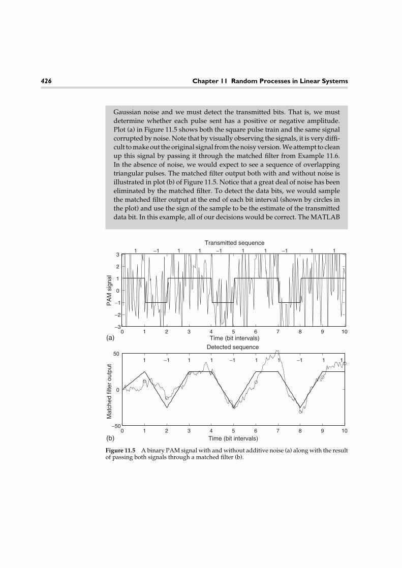
426 Chapter 11 Random Processes in Linear Systems
Gaussian noise and we must detect the transmitted bits. That is, we mustdetermine whether each pulse sent has a positive or negative amplitude.Plot (a) in Figure 11.5 shows both the square pulse train and the same signalcorrupted by noise. Note that by visually observing the signals, it is very diffi-cult to make out the original signal from the noisy version. We attempt to cleanup this signal by passing it through the matched filter from Example 11.6.In the absence of noise, we would expect to see a sequence of overlappingtriangular pulses. The matched filter output both with and without noise isillustrated in plot (b) of Figure 11.5. Notice that a great deal of noise has beeneliminated by the matched filter. To detect the data bits, we would samplethe matched filter output at the end of each bit interval (shown by circles inthe plot) and use the sign of the sample to be the estimate of the transmitteddata bit. In this example, all of our decisions would be correct. The MATLAB
0 1 2 3 4 5 6 7 8 9 10−3
−2
−1
0
1
2
3
PA
M s
igna
l
0 1 2 3 4 5 6 7 8 9 10−50
0
50
Mat
ched
filte
r ou
tput
Time (bit intervals)
1 −1 1 1 −1 1 1 −1 1 1
1 −1 1 1 −1 1 1 −1 1 1
Detected sequence
Time (bit intervals)
Transmitted sequence
(a)
(b)
Figure 11.5 A binary PAM signal with and without additive noise (a) along with the resultof passing both signals through a matched filter (b).

11.6 The Wiener Filter 427
code used to generate these signals follows. This is just a modified version ofthe code used to generate the PAM signal in Example 10.14.
N=10; % Number of bit intervals.
Ns=25; % Number of time samples per bit.
t=([1:Ns]-0.5)/Ns; % Time axis for pulse shape.
p=ones(size(t)); % Square pulse shape.
d=sign(rand(1,N)-0.5); % Random data bits.
X(1:Ns:(Ns*(N-1)+1))=d;
X=conv(X,p); % PAM signal with pulse shape.
sigma=sqrt(Ns/10); % Noise strength.
noise=sigma*randn(size(X)); % Gaussian noise.
R=X+noise;
subplot(2,1,1) % Plot clean and noisy signals.
x_axis=[1:length(R)]/Ns;
plot(x_axis,R, x_axis,X)
axis([0 N -3 3])
h=fliplr(p); % Matched filter impulse response.
z=conv(R,h); % Noisy output of matched filter.
z2=conv(X,h); % Noise-free MF output.
zs=z(Ns*[1:N]); % Sample matched filter outputs.
subplot(2,1,2) % Plot matched filter output.
x_axis=[1:length(z)]/Ns;
plot(x_axis,z,‘-’,x_axis,z2,‘-’,[1:N],zs,‘o’)
11.6 The Wiener Filter
In this section, we consider another filter design problem that involves removingthe noise from a sum of a desired signal plus noise. In this case, the desired signalis also a random process (rather than a known, deterministic signal as in the lastsection) and the goal here is to estimate the desired part of the signal plus noise.In its most general form, the problem is stated as follows. Given a random processX(t), we want to form an estimate Y(t) of some other zero-mean process Z(t) basedon observation of some portion of X(t). We require the estimator to be linear. Thatis, we will obtain Y(t) by filtering X(t). Hence,
Y(t) =∫ ∞
−∞h(t − u)X(u) du. (11.39)

428 Chapter 11 Random Processes in Linear Systems
We want to design the filter to minimize the mean square error
E[ε2(t)] = E[(Z(t) − Y(t))2]. (11.40)
In this section, we will consider the special case where the observation consistsof the process we are trying to estimate plus independent noise. That is X(t) =Z(t) + N(t). We observe X(t) for some time interval t ∈ (t1, t2) and based on thatobservation, we will form an estimate of Z(t). Consider a few special cases:
• Case I. If (t1, t2) = (−∞, t), then we have a filtering problem in which wemust estimate the present based on the entire past. We may also have (t1, t2) =(t − to, t), in which case we have a filtering problem where we must estimatethe present based on the most recent past.
• Case II. If (t1, t2) = (−∞, ∞), then we have a smoothing problem where wemust estimate the present based on a noisy version of the past, present, andfuture.
• Case III. If (t1, t2) = (−∞, t − to), then we have a prediction problem where wemust estimate the future based on the past and present.
All of these cases can be cast in the same general framework and a single resultwill describe the optimal filter for all cases. In order to derive the optimal filter, itis easier to view the problem in discrete time and then ultimately pass to the limitof continuous time. Hence, we reformulate the problem in discrete time. Given anobservation of the discrete time process X[n] = Z[n]+N[n] over some time intervaln ∈ [n1, n2], we wish to design a filter h[n] such that the linear estimate
Y[n] =n2∑
k=n1
h[n − k]X[k] (11.41)
minimizes the mean square error E[ε2[n]] = E[(Z[n] − Y[n])2].The filter h[n] can be viewed as a sequence of variables. We seek to jointly
optimize with respect to each variable in that sequence. This can be done by dif-ferentiating with respect to each variable and setting the resulting equations equalto zero:
ddh[m]E[ε2[n]] = 2E
[ε[n] d
dh[m]ε[n]]
= 0, m ∈ [n − n2, n − n1]. (11.42)
Noting that
ddh[m]ε[n] = d
dh[m] (Z[n] − Y[n]) = − ddh[m]Y[n] = −X[n − m], (11.43)
the system of equations to solve becomes
E[ε[n]X[n − m]] = 0, for m ∈ [n − n1, n − n2]. (11.44)

11.6 The Wiener Filter 429
Equivalently, this can be rewritten as
E[ε[n]X[m]] = 0, for m ∈ [n1, n2]. (11.45)
In summary, the filter that minimizes the mean square error will cause the observeddata to be orthogonal to the error. This is known as the orthogonality principle.Applying the orthogonality principle, we have
E[ε[n]X[m]] = E
Z[n] −
n2∑k=n1
h[n − k]X[k]X[m]
= 0. (11.46)
Assuming all the processes involved are jointly WSS, these expectations can bewritten in terms of autocorrelation and cross correlation functions as
n2∑k=n1
h[n − k]RXX[k − m] = RZX[n − m], m ∈ [n1, n2], (11.47)
or equivalently,
n−n1∑i=n−n2
h[i]RXX[k − i] = RZX[k], k ∈ [n − n2, n − n1]. (11.48)
These equations are known as the Wiener-Hopf equations, the normal equations,or the Yule-Walker equations. The resulting filter found by solving this system ofequations is known as the Wiener filter.
A similar result can be found for continuous time systems by applying theorthogonality principle in continuous time. Given an observation of X(t) over thetime interval (t1, t2), the orthogonality principle states that the filter that minimizesthe mean square prediction error will satisfy
E[ε(t)X(s)] = 0, for s ∈ (t1, t2). (11.49)
This produces the continuous-time version of the Wiener-Hopf equation,∫ t−t1
t−t2
h(v)RXX(τ − v) dv = RZX(τ ), τ ∈ (t − t2, t − t1). (11.50)
The techniques used to solve the Wiener-Hopf equation depend on the nature ofthe observation interval. For example, consider the smoothing problem where theobservation interval is (t1, t2) = (−∞, ∞). In that case, the Wiener-Hopf equationbecomes ∫ ∞
−∞h(v)RXX(τ − v) dv = RZX(τ ). (11.51)

430 Chapter 11 Random Processes in Linear Systems
The left-hand side of the equation is a convolution and the integral equation caneasily be solved using Fourier transforms. Taking a Fourier transform of both sidesof the equation results in
H(f )SXX(f ) = SZX(f ) ⇒ H(f ) = SZX(f )SXX(f )
. (11.52)
Note also that if the noise is zero-mean and independent of Z(t), then RZX(τ ) =RZZ(τ ) and RXX(τ ) = RZZ(τ ) + RNN(τ ). The transfer function of the Wiener filterfor the smoothing problem then becomes
H(f ) = SZZ(f )SZZ(f ) + SNN(f )
. (11.53)
EXAMPLE 11.8: Suppose the desired signal Z(t) has a spectral den-sity of
SZZ(f ) = 11 + f 2
and the noise is white with a PSD of SNN(f ) = 1. Then the Wiener filterfor the smoothing problem has the form
H(f ) =1
1 + f 2
11 + f 2 + 1
= 12 + f 2 .
The corresponding impulse response is
h(t) = π√2
exp(−√8π |t|).
Note that this filter is not causal. This is due to the nature of the smooth-ing problem, whereby we estimate the present based on past, present,and future.
Next, consider the filtering problem where the observation interval is (t1, t2) =(−∞, t). In this case, the Wiener-Hopf equation becomes
∫ ∞
0h(v)RXX(τ − v) dv = RZX(τ ), τ ∈ (0, ∞) (11.54)
It is emphasized now that the left-hand side of the equation is not a convolutionsince the lower limit of the integral is not −∞. The resulting integral equation

11.6 The Wiener Filter 431
is much trickier to solve than in the case of the smoothing problem. In order todevelop a procedure for solving this general equation, consider the special casewhen RXX(τ ) = δ(τ ). In that case, the preceding integral equation becomes
h(τ ) = RZX(τ ) for τ > 0. (11.55)
Because we are estimating the present based on observing the past, the filter mustbe causal and thus its impulse response must be zero for negative time. Thus, forthe special case when RXX(τ ) = δ(τ ), the Wiener filter is h(τ ) = RZX(τ )u(τ ).
This example in itself is not very interesting since we would not expect X(t) tobe white, but it does help to find the general solution to the Wiener-Hopf equation.First, before estimating Z(t), suppose we pass the input X(t) through a causal filterwith a transfer function 1/G(f ). Call the output X(t). If G(f ) is chosen such that|G(f )|2 = SXX(f ), then the process X(t) will be a white process and the filter iscalled a whitening filter. We can then use the result of the previous special case toestimate Z(t) based on the white process X(t). Hence, we are designing the Wienerfilter in two stages as illustrated in Figure 11.6.
To find the impulse response of the second filter, we start with the result thath2(τ ) = RZX(τ )U(τ ). Also, since X(t) can be written as X(t) = X(t) ∗ h1(t), then
SZX(f ) = SZX(f )H∗1 (f ). (11.56)
The resulting quantities needed to form the second filter are then
SZX(f ) = SZX(f )G∗(f )
←→ RZX(τ ) = F−1{
SZX(f )G∗(f )
}. (11.57)
To construct the whitening filter, we need to find a G(f ) such that (1) H1(f ) = 1/G(f )is causal, and (2) |G(f )|2 = SXX(f ). The procedure for doing this is known as spectralfactorization. Since SXX(f ) is a PSD and thus is an even function of f , it will factorin the form
SXX(f ) = G(f )G ∗ (f ), (11.58)
Whiteningfilter
Wiener filterfor white input
X(t ) X~
(t ) Y(t )H1(f ) = 1
G(f )H2(f )
Figure 11.6 Constructing the Wiener filter for the filtering problem as a cascade of twofilters.

432 Chapter 11 Random Processes in Linear Systems
where half of the poles and zeros are assigned to G(f ) and the other half are assignedto G∗(f ). In order to be sure that H1(f ) is causal, we assign to G(f ) those zeros inthe upper half-plane. As will be shown in the next example, it is also important toassign poles from the upper half-plane to G(f ) as well.
EXAMPLE 11.9: For this example, let X(t) = Z(t) + N(t), where N(t) iswhite noise with a spectral density of SNN(f ) = 1 and independent ofZ(t), which has a spectral density of
SZZ(f ) = 31 + (2π f )2 .
Note also that
SZX(f ) = SZZ(f ) and SXX(f ) = SZZ(f ) + SNN(f ) = 31 + (2π f )2 + 1
= 4 + (2π f )2
1 + (2π f )2 = (2 + j2π f )(2 − j2π f )(1 + j2π f )(1 − j2π f )
.
A pole-zero plot for the PSD function SXX(f ) is shown in Figure 11.7.We assign the poles and zeros in the upper half-plane to the functionG(f ) (and hence the poles and zeros in the lower half-plane go to G∗(f )).This results in
G(f ) = 2 + j2π f1 + j2π f
=⇒ H1(f ) = 1 + j2π f2 + j2π f
= 1 − 12 + j2π f
.
The corresponding impulse response is
h1(t) = δ(t) − e−2tu(t).
*
*
o
o
* = poleo = zero
Im(f )
Re(f )
Figure 11.7 Pole-zero plot for the PSD function of Example 11.9.

11.6 The Wiener Filter 433
As desired, the whitening filter is causal. To find the form of the secondfilter, we first calculate the cross spectral density between X(t) and Z(t):
SZX(f ) = SZX(f )H∗1 (f ) = 3
1 + (2π f )21 − j2π f2 − j2π f
= 3(1 + j2π f )(2 − j2π f )
= 11 + j2π f
+ 12 − j2π f
.
Taking an inverse Fourier transform, the cross correlation function is
RZX(τ ) = e−τ u(τ ) + e2τ u(−τ ).
The impulse response of the second filter is then given by
h2(τ ) = RZX(τ )u(τ ) = e−τ u(τ ).
When the actual Wiener filter is implemented, there is no reason thefilter has to be implemented as a cascade of two filters. We did thisfor ease of determining the filter. Combining these two filters into oneproduces
H(f ) = H1(f )H2(f ) =(
1 + j2π f2 + j2π f
)(1
1 + j2π f
)
= 12 + j2π f
←→ h(t) = e−2tu(t).
It can be easily verified that this filter does indeed satisfy the Wiener-Hopf equation.
Note, we also could have chosen G(f ) = (2 + j2π f )/(1 − j2π f ), andH1(f ) = 1/G(f ) would still have been causal:
H1(f ) = 1 − j2π f2 + j2π f
= −1 + 32 + j2π f
←→ h1(t) = −δ(t) + 3e−2tu(t).
In this case,
SZX(f ) = SZX(f )H∗1 (f ) = 3
1 + (2π f )21 + j2π f2 − j2π f
= 3(1 − j2π f )(2 − j2π f )
= 31 − j2π f
+ −32 − j2π f
.
←→ RZX(τ ) = 3eτ u(−τ ) − 3e2τ u(−τ )
This leads to h2(t) = 0!! Thus, we see it is important to assign both polesand zeros from the upper half-plane to G(f ).
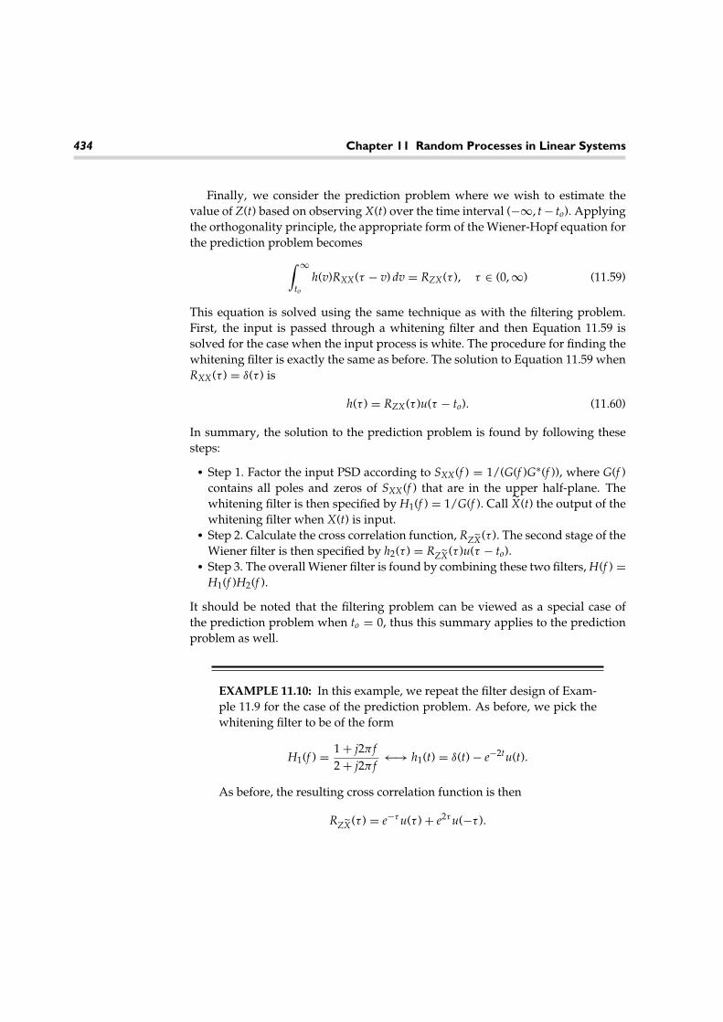
434 Chapter 11 Random Processes in Linear Systems
Finally, we consider the prediction problem where we wish to estimate thevalue of Z(t) based on observing X(t) over the time interval (−∞, t − to). Applyingthe orthogonality principle, the appropriate form of the Wiener-Hopf equation forthe prediction problem becomes
∫ ∞
to
h(v)RXX(τ − v) dv = RZX(τ ), τ ∈ (0, ∞) (11.59)
This equation is solved using the same technique as with the filtering problem.First, the input is passed through a whitening filter and then Equation 11.59 issolved for the case when the input process is white. The procedure for finding thewhitening filter is exactly the same as before. The solution to Equation 11.59 whenRXX(τ ) = δ(τ ) is
h(τ ) = RZX(τ )u(τ − to). (11.60)
In summary, the solution to the prediction problem is found by following thesesteps:
• Step 1. Factor the input PSD according to SXX(f ) = 1/(G(f )G∗(f )), where G(f )contains all poles and zeros of SXX(f ) that are in the upper half-plane. Thewhitening filter is then specified by H1(f ) = 1/G(f ). Call X(t) the output of thewhitening filter when X(t) is input.
• Step 2. Calculate the cross correlation function, RZX(τ ). The second stage of theWiener filter is then specified by h2(τ ) = RZX(τ )u(τ − to).
• Step 3. The overall Wiener filter is found by combining these two filters, H(f ) =H1(f )H2(f ).
It should be noted that the filtering problem can be viewed as a special case ofthe prediction problem when to = 0, thus this summary applies to the predictionproblem as well.
EXAMPLE 11.10: In this example, we repeat the filter design of Exam-ple 11.9 for the case of the prediction problem. As before, we pick thewhitening filter to be of the form
H1(f ) = 1 + j2π f2 + j2π f
←→ h1(t) = δ(t) − e−2tu(t).
As before, the resulting cross correlation function is then
RZX(τ ) = e−τ u(τ ) + e2τ u(−τ ).
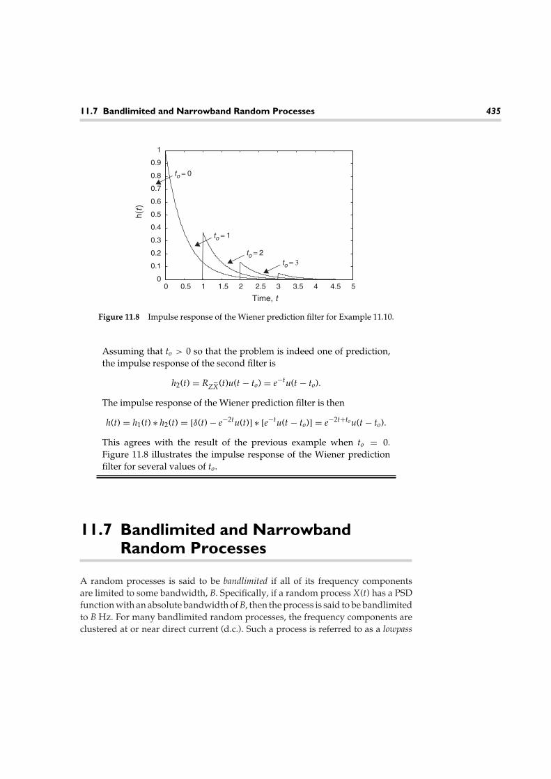
11.7 Bandlimited and Narrowband Random Processes 435
0 0.5 1 1.5 2 2.5 3 3.5 4 4.5 50
0.1
0.2
0.3
0.4
0.5
0.6
0.7
0.8
0.9
1
Time, t
h(t)
to = 0
to = 1
to = 2to = 3
Figure 11.8 Impulse response of the Wiener prediction filter for Example 11.10.
Assuming that to > 0 so that the problem is indeed one of prediction,the impulse response of the second filter is
h2(t) = RZX(t)u(t − to) = e−tu(t − to).
The impulse response of the Wiener prediction filter is then
h(t) = h1(t) ∗ h2(t) = [δ(t) − e−2tu(t)] ∗ [e−tu(t − to)] = e−2t+to u(t − to).
This agrees with the result of the previous example when to = 0.Figure 11.8 illustrates the impulse response of the Wiener predictionfilter for several values of to.
11.7 Bandlimited and NarrowbandRandom Processes
A random processes is said to be bandlimited if all of its frequency componentsare limited to some bandwidth, B. Specifically, if a random process X(t) has a PSDfunction with an absolute bandwidth of B, then the process is said to be bandlimitedto B Hz. For many bandlimited random processes, the frequency components areclustered at or near direct current (d.c.). Such a process is referred to as a lowpass
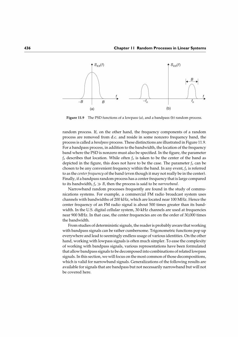
436 Chapter 11 Random Processes in Linear Systems
SXX(f ) SXX(f )
f f
−B
B
(a) (b)
B −fo fo
Figure 11.9 The PSD functions of a lowpass (a), and a bandpass (b) random process.
random process. If, on the other hand, the frequency components of a randomprocess are removed from d.c. and reside in some nonzero frequency band, theprocess is called a bandpass process. These distinctions are illustrated in Figure 11.9.For a bandpass process, in addition to the bandwidth, the location of the frequencyband where the PSD is nonzero must also be specified. In the figure, the parameterfo describes that location. While often fo is taken to be the center of the band asdepicted in the figure, this does not have to be the case. The parameter fo can bechosen to be any convenient frequency within the band. In any event, fo is referredto as the center frequency of the band (even though it may not really be in the center).Finally, if a bandpass random process has a center frequency that is large comparedto its bandwidth, fo � B, then the process is said to be narrowband.
Narrowband random processes frequently are found in the study of commu-nications systems. For example, a commercial FM radio broadcast system useschannels with bandwidths of 200 kHz, which are located near 100 MHz. Hence thecenter frequency of an FM radio signal is about 500 times greater than its band-width. In the U.S. digital cellular system, 30-kHz channels are used at frequenciesnear 900 MHz. In that case, the center frequencies are on the order of 30,000 timesthe bandwidth.
From studies of deterministic signals, the reader is probably aware that workingwith bandpass signals can be rather cumbersome. Trigonometric functions pop upeverywhere and lead to seemingly endless usage of various identities. On the otherhand, working with lowpass signals is often much simpler. To ease the complexityof working with bandpass signals, various representations have been formulatedthat allow bandpass signals to be decomposed into combinations of related lowpasssignals. In this section, we will focus on the most common of those decompositions,which is valid for narrowband signals. Generalizations of the following results areavailable for signals that are bandpass but not necessarily narrowband but will notbe covered here.

11.7 Bandlimited and Narrowband Random Processes 437
Suppose a random process Z(t) is narrowband. Then Z(t) can be expressed interms of two lowpass processes X(t) and Y(t) according to
Z(t) = X(t) cos(ωot) − Y(t) sin(ωot). (11.61)
The two processes X(t) and Y(t) are referred to as the inphase (I) and quadrature (Q)components of Z(t). Although it is not proven here, the equality in the previousequation is in the mean-square sense. That is,
E[{Z(t) − (X(t) cos(ωot) − Y(t) sin(ωot))}2] = 0. (11.62)
This Cartesian representation of the narrowband random process can also bereplaced by a polar representation of the form
Z(t) = R(t) cos(ωot + �(t)), (11.63)
where R(t) is called the real envelope of Z(t) and �(t) is the excess phase. We nextdescribe the relationship between the statistics of the I and Q components and thestatistics of the original random process.
The I and Q components of a signal can be extracted using the system shownin Figure 11.10. The passbands of the lowpass filters need to be large enough topass the desired components (i.e., > B/2 Hz) but not so large as to pass the doublefrequency components produced by the mixers (at and around 2fo Hz). For nar-rowband signals where fo � B, the filters can be very loosely designed, and hencewe do not need to worry too much about the particular forms of these filters. Tosee how this network functions, consider the output of the upper mixer:
2Z(t) cos(ωot) = 2{X(t) cos(ωot) − Y(t) sin(ωot)} cos(ωot)
= X(t){1 + cos(2ωot)} − Y(t) sin(2ωot). (11.64)
×
×
Low passFilter
Low passFilter
Z(t )
–2 sin(ωot )
2 cos(τot )
Y(t )
X(t )
Figure 11.10 Network for decomposing a narrowband process into its I and Q components.

438 Chapter 11 Random Processes in Linear Systems
After passing this through the lowpass filter, the terms involving the double fre-quencies will be attenuated and the output of the upper LPF is indeed X(t). Similarcalculations reveal that Y(t) is indeed the output of the lower branch.
Next we calculate PSDs involving the I and Q components. Consider first,multiplication of the process Z(t) by a sinusoid. Let A(t) = 2Z(t) cos(ωot). Theautocorrelation function of A(t) is easily calculated to be
RAA(t, t + τ ) = 2RZZ(τ ){cos(ωoτ ) + cos(2ωot + ωoτ )}. (11.65)
Note that the process A(t) is not WSS. In order to compute the PSD of a process thatis not stationary, we must first take the time average of the autocorrelation function(with respect to t) so that the result will be a function of τ only. This time-averagedautocorrelation function works out to be
〈RAA(t, t + τ )〉 = 2RZZ(τ ){cos(ωoτ ) + 〈cos(2ωot + ωoτ )〉} = 2RZZ(τ ) cos(ωoτ ).(11.66)
At this point, the PSD of A(t) can then be found through Fourier transforma-tion to be
SAA(f ) = SZZ(f − fo) + SZZ(f + fo). (11.67)
Recall that the process Z(t) was assumed to be narrowband. That is, its PSD hascomponents near fo and −fo. After shifting by fo, the term SZZ(f −fo) has componentsnear d.c. and also near 2fo. The components near d.c. will pass through the filterwhile those at and around 2fo will be attenuated. Similarly, SZZ(f + fo) will haveterms near d.c. that will pass through the filter and terms near −2fo that will not.This is illustrated in Figure 11.11. For notational convenience, let LP{} denote the
SAA(f )
f
−
B
LPF
B2
2f0B2
–2f0
Figure 11.11 PSD of the input to the LPF in the I branch.
11.7 Bandlimited and Narrowband Random Processes 439
lowpass part of a quantity. Then the PSD of the inphase component of a narrowbandprocess can be written in terms of the PSD of the original process as
SXX(f ) = L. P.{SZZ(f − fo) + SZZ(f + fo)}. (11.68)
Following a similar set of steps, the PSD of the Q component is found to be identicalto the I component. That is,
SYY(f ) = SXX(f ) = L. P.{SZZ(f − fo) + SZZ(f + fo)}. (11.69)
The cross spectral density can also be calculated in a manner similar to the PSDs.The result is
SXY(f ) = j L. P.{SZZ(f − fo) − SZZ(f + fo)}. (11.70)
It is noted that if the PSD function SZZ(f ) is symmetric about f = fo, then the crossspectral density works out to be zero. In that case, the I and Q components areorthogonal (since RXY(τ ) = 0). Furthermore, if the process Z(t) is zero-mean, thenthe I and Q components will also be zero-mean. In this case, the I and Q componentsare then uncorrelated. Finally, if in addition Z(t) is a Gaussian random process, thenthe I and Q components are also statistically independent. In summary, we haveproven the results of the following theorem.
THEOREM 11.4: For a narrowband process Z(t), the PSDs involving the I and Qcomponents X(t) and Y(t) are given by
SYY(f ) = SXX(f ) = L. P.{SZZ(f − fo) + SZZ(f + fo)}, (11.71a)
SXY(f ) = j L. P.{SZZ(f − fo) − SZZ(f + fo)}. (11.71b)
If Z(t) is a zero-mean Gaussian random process and its PSD is symmetric aboutf = fo, then the I and Q components are statistically independent.
EXAMPLE 11.11: Suppose zero-mean white Gaussian noise with a PSDof No/2 is passed through an ideal BPF with a bandwidth of B Hz toproduce the narrowband noise process Z(t) as shown in Figure 11.12.The I and Q components will then have a PSD that is given by
SYY(f ) = SXX(f ) = No rect(f /B).
The corresponding autocorrelation functions are
RXX(τ ) = RYY(τ ) = NoB sinc(Bτ ).

440 Chapter 11 Random Processes in Linear Systems
Ideal BPFBW=B
Whitenoise –fo
No / 2
SZZ(f ) SXX(f ) = SYY(f )B No
B2
(a) (b) (c)
Z(t )
fo
f f
B2
–
Figure 11.12 Generation of a narrowband noise process (a), its PSD function (b), and thePSD function of the I and Q components (c).
Since the PSD of Z(t) is symmetric about f − fo, the cross PSD is zero andhence the I and Q components are independent.
11.8 Complex Envelopes
When working with narrowband random processes, it is convenient to combinethe I and Q components into a single lowpass random process whose real part is theI component and whose imaginary part is the Q component. The resulting randomprocess is a complex lowpass random process.
DEFINITION 11.3: For a narrowband process, Z(t), with I and Q components,X(t) and Y(t), respectively, the complex envelope, Gz(t), is defined as
Gz(t) = X(t) + jY(t). (11.72)
With this definition, the random process is written in terms of its complex envelopeaccording to
Z(t) = Re[Gz(t)e jωot]. (11.73)
The properties developed in the previous section for the I and Q components ofa narrowband random process can be used to determine equivalent properties forthe complex envelope. To be consistent with the definitions for complex randomvariables given in Chapter 5, we define the autocorrelation function of a complexrandom process as follows.

11.8 Complex Envelopes 441
DEFINITION 11.4: For any complex random process G(t), the autocorrelationfunction is defined as2
RGG(t, t + τ ) = 12
E[G(t)G∗(t + τ )]. (11.74)
If G(t) represents the complex envelope of a narrowband random process and theI and Q components are jointly WSS, then this autocorrelation function will be afunction of only τ . Also, the corresponding PSD can be found through Fouriertransformation:
SGG(f ) = F[RGG(τ )]. (11.75)
Using this definition together with the properties developed in the previous section,the autocorrelation function for a complex envelope is found to be
RGG(τ ) = 12
E[(X(t) + jY(t))(X(t + τ ) − jY(t + τ ))]
= 12
RXX(τ ) + 12
RYY(τ ) + j2
RYX(τ ) − j2
RXY(τ ). (11.76)
For the case where the I and Q components are orthogonal, this reduces to
RGG(τ ) = 12
RXX(τ ) + 12
RYY(τ ) = RXX(τ ) = RYY(τ ). (11.77)
The corresponding PSD is then
SGG(f ) = SXX(f ) = SYY(f ) = L. P.{SZZ(f − fo) + SZZ(f + fo)}. (11.78)
Hence, the complex envelope has the same PSD and autocorrelation function asthe I and Q components. It is left as an exercise for the reader to show that theautocorrelation and PSD functions of the original narrowband process can be foundfrom those of the complex envelope according to
SZZ(f ) = 12
SGG(f − fo) + 12
SGG(−f − fo), (11.79)
RZZ(τ ) = Re[RGG(τ )e jωoτ ]. (11.80)
2The same disclaimer must be made here as in Definition 5.13. Many texts do not includethe factor of 1/2 in the definition of the autocorrelation function for complex randomprocesses, and hence the reader should be aware that there are two different definitionsprevalent in the literature.

442 Chapter 11 Random Processes in Linear Systems
11.9 Engineering Application: An AnalogCommunication System
A block diagram of a simple amplitude modulation (AM) analog communicationsystem is shown in Figure 11.13. A message (usually voice or music) is representedas a random process X(t) with some bandwidth B. This message is modulated ontoa carrier using amplitude modulation. The resulting AM signal is of the form
SAM(t) = [Ao + X(t)] cos(ωct + �). (11.81)
In AM, a bias, Ao, is added to the message and the result forms the time-varyingamplitude of a radio frequency (RF) carrier. In order to allow for envelope detectionat the receiver, the bias must satisfy Ao > max |X(t)|. Some example waveformsare shown in Figure 11.14. Note that due to the process of modulation, the AMsignal now occupies a bandwidth of 2B. The modulated RF signal is transmittedusing an antenna and propagates through the environment to the receiver whereit is picked up with a receiving antenna.
To study the effects of noise on the AM system, we ignore other sources ofcorruption (e.g., interference, distortion) and model the received signal as simplya noisy version of the transmitted signal,
R(t) = SAM(t) + Nw(t), (11.82)
where Nw(t) is a Gaussian white noise process with a PSD of N0/2. To limit theeffects of noise, the received signal is passed through a BPF whose passband ischosen to allow the AM signal to pass while removing as much of the noise aspossible. This receiver filter is taken to be an ideal bandpass filter whose bandwidthis 2B. The output of the filter is then modeled as an AM signal plus narrowbandnoise:
Z(t) = SAM(t) + Nx(t) cos(ωct + �) − Ny(t) sin(ωct + �)
= [Ao + X(t) + Nx(t)] cos(ωct + �) − Ny(t) sin(ωct + �). (11.83)
Messagesource
Modulator(AM) + Envelope
detectorX(t ) SAM (t )
R (t ) Z (t ) Xd (t )
Nw (t )
IdealBPF
Figure 11.13 A block diagram of an amplitude modulation (AM) communications system.

11.9 Engineering Application: An Analog Communication System 443
0 0.5 1 1.5 2 2.5 3 3.5 4 4.5 5–3
–2
–1
0
1
2
3
mes
sage
, X(t
)
time
0 0.5 1 1.5 2 2.5 3 3.5 4 4.5 5
–6
–4
–2
0
2
4
6
AM
sig
nal,
SA
M(t
)
time
Figure 11.14 A sample message and the corresponding AM signal.
The envelope detector is a device that outputs the real envelope of the input. Hence,for the preceding input, the demodulated output will be
Xd(t) =√
(Ao + X(t) + Nx(t))2 + (Ny(t))2. (11.84)
In its normal operating mode, the desired portion of the filter output will generallybe much stronger than the noise. In this case, we observe that most of the time Ao +X(t) + Nx(t) � Ny(t) so that the demodulated output can be well approximated by
Xd(t) ≈ Ao + X(t) + Nx(t). (11.85)
The DC component can easily be removed and hence X(t) represents the desiredcomponent of the demodulated output and Nx(t) is the undesired (noise) compo-nent. The power in the desired component depends on the message and we simplywrite it as E[X2(t)]. The I-component of the narrowband noise has a spectral den-sity equal to N0 for |f | < B (and zero otherwise). Hence, the noise power at the

444 Chapter 11 Random Processes in Linear Systems
demodulator output is 2N0B. The resulting signal-to-noise ratio at the output ofthe AM systems is
SNR = E[X2(t)]2N0B
. (11.86)
It is common to express this SNR in terms of the transmitted power required tosupport the AM modulator. For an AM signal of the form in Equation 11.81, thetransmitted power is
PT = E[(Ao + X(t))2 cos2(ωct + �)] = E[(Ao + X(t))2]E[cos2(ωct + �)], (11.87)
assuming the carrier phase is independent of the message. If the message is azero-mean random process (which is usually the case), this expression simplifies to
PT = A20 + E[X2(t)]
2. (11.88)
Using this relationship, the SNR of the AM system can then be expressed as
SNR = E[X2(t)]A2
0 + E[X2(t)]PT
N0B. (11.89)
The factor,
ηAM = E[X2(t)]A2
0 + E[X2(t)] , (11.90)
is known as the modulation efficiency of AM and is usually expressed as a per-centage. Note that due to the requirement that Ao > max |X(t)|, the modulationefficiency of AM must be less than 50 percent (which would occur for square wavemessages). For a sinusoidal message, the modulation efficiency would be no morethan 33 percent while for a typical voice or music signal, the modulation efficiencymight be much smaller.
EXAMPLE 11.12: The MATLAB code that follows simulates themodulation and demodulation of an AM signal. The message sig-nal is the sum of two sinusoids (one at 100 Hz and one at 250 Hz).For this example, the carrier frequency is taken to be fc = 100 kHz.
We’ve added noise to the AM signal to produce a typical received signal asshown in plot (a) of Figure 11.15. To demodulate the signal, we decomposethe received signal into its I and Q components using the technique illustratedin Figure 11.9. The lowpass filter we used was a second-order Butterworthfilter with a cutoff frequency of 400 Hz, but the particular form of the filter

11.9 Engineering Application: An Analog Communication System 445
0 0.005 0.01 0.015 0.02 0.025–10
–5
0
5
10
AM
sig
nal
0 0.005 0.01 0.015 0.02 0.025–1
–0.5
0
0.5
1
Mes
sage
Time (sec)
(a)
(b)
Figure 11.15 An AM signal corrupted by noise (a) along with a comparison of the originalmessage and the demodulated message (b).
is not crucial. Once these components are found, the real envelope is com-puted according to R(t) = √
X2(t) + Y2(t). Our estimate of the message is thena scaled version of this envelope with the DC component removed. Plot (b) inFigure 11.15 shows the original message (dashed) and the recovered message(solid).
fc=100000; % Carrier frequency.
dt=1/(4*fc); % Sampling interval.
t=[0:dt:0.025];
f1=100; f2=250;
m=sin(2*pi*f1*t)+2*cos(2*pi*f2*t); % Message signal (two
tones).
s=(m+1+max(abs(m))).*cos(2*pi* % AM signal.
(fc*t+rand(1)));
s=s+randn(1,length(s)); % Noisy AM signal.
subplot(2,1,1)
plot(t,s); ylabel(‘AM signal’);

446 Chapter 11 Random Processes in Linear Systems
f0=400;
a=2*pi*f0/sqrt(2);
h=exp(-a*t).*sin(a*t); % Second-order lowpass filter
% with cut-off frequency at f0.
temp=s.*cos(2*pi*fc*t);
x=conv(temp,h)*dt; % I component.
temp=s.*sin(2*pi*fc*t);
y=conv(temp,h)*dt; % Q component.
r=sqrt(x.∧2+y.∧2); % Real envelope.
r=r(1:length(t));
mhat=r-sum(r)/length(r);
subplot(2,1,2)
plot(t,mhat/max(mhat),‘b’,t,m/max(m),‘g--’)
axis([0 max(t) -1.1 1.1])
ylabel(‘Message’); xlabel(‘time (sec)’)
Exercises11.1 A white noise process, X(t), with a power spectral density (PSD) of
SXX(f ) = No/2 is passed through a finite time integrator whose outputis given by
Y(t) =∫ t
t−to
X(u) du.
Find the following:
(a) the PSD of the output process,
(b) the total power in the output process,
(c) the noise equivalent bandwidth of the integrator (filter).
11.2 A certain linear time-invariant system has an input/output relationshipgiven by
Y(t) = X(t) − X(t − to)to
.
(a) Find the output autocorrelation, RYY(τ ), in terms of the input autocor-relation, RXX(τ ).

Exercises 447
(b) Find the output PSD, SYY(f ), in terms of the input PSD, SXX(f ).(c) Does your answer to part (b) make sense in the limit as to → 0?
11.3 The output Y(t) of a linear filter is c times the input X(t). Show that RYY(τ ) =c2RXX(τ ).
11.4 The output Y(t) of a filter is given in terms of its input X(t) by Y(t) =X(t) + X(t − to) + X(t − 2to).
(a) Determine RYY(τ ) as a function of RXX(τ ).(b) Find E[Y2(t)].
11.5 Is the following function a valid discrete-time autocorrelation function?Justify your answer.
RXX[k] =
1 k = 134
k = ±3
0 otherwise
.
11.6 A discrete random sequence X[n] is the input to a discrete linear filter h[n].The output is Y[n]. Let Z[n] = X[n + i] − Y[n]. Find E[Z2[n]] in terms ofthe autocorrelation functions for X[n] and Y[n] and the cross correlationfunction between X[n] and Y[n].
11.7 The unit impulse response of a discrete linear filter is h[n] = anu[n], where|a| < 1. The autocorrelation function for the input random sequence is
RXX[k] ={
1 k = 0
0 otherwise.
Determine the cross correlation function between the input and outputrandom sequences.
11.8 Find the PSD of a discrete random sequence with the following autocor-relation function: RXX[k] = a(b|k|), where |b| < 1.
11.9 A discrete time linear filter has a unit pulse response h[n]. The input tothis filter is a random sequence with uncorrelated samples. Show that theoutput power spectral density is real and nonnegative.
11.10 Consider a nonlinear device such that the output is Y(t) = aX2(t), where theinput X(t) consists of a signal plus a noise component, X(t) = S(t) + N(t).
448 Chapter 11 Random Processes in Linear Systems
Determine the mean and autocorrelation function for Y(t) when the signalS(t) and the noise N(t) are both Gaussian random processes and wide sensestationary (WSS) with zero mean, and S(t) is independent of N(t).
11.11 Calculate the spectrum for Y(t) in Exercise 11.10 if
SSS(f ) = A2
4[δ(f + fc) + δ(f − fc)],
and
SNN(f ) =
No
2fc − B
2< |f | < fc + B
20 otherwise
.
11.12 If the input to a linear filter is a random telegraph process with c zerocrossings per second and an amplitude A, determine the output powerspectral density. The filter impulse response is h(t) = b exp(−at) u(t).
11.13 The input to a linear filter is a random process with the followingautocorrelation function:
RXX(τ ) = Aωo
π
sin(ωoτ )ωoτ
.
The impulse response of the filter is of the same form and is
h(t) = ω1
π
sin(ω1t)ω1t
.
Determine the autocorrelation function of the filter output for ωo ≥ ω1 andfor ωo < ω1.
11.14 The power spectrum at the input to an ideal bandpass filter is
SXX(f ) = a1 + (f /fo)2 .
Let the transfer function for the ideal bandpass filter be
H(f ) ={
b for f1 < |f | < f20 otherwise
.
Determine the autocorrelation function of the output. You may have tomake a reasonable approximation to obtain a simplified form. Assumethat f1 − f2 � fo and (f2 − f1)/f2 � 1.

Exercises 449
11.15 A random process with a PSD of SXX(f ) = 1/(1 + f 2) is input to a filter.The filter is to be designed so that the output process is white (constantPSD). This filter is called a whitening filter.
(a) Find the transfer function of the whitening filter for this input process.Be sure that the filter is causal.
(b) Sketch a circuit that will realize this transfer function.
11.16 White Gaussian noise is input to an RC lowpass filter.
(a) At what sampling instants is the output independent of the input attime t = t1?
(b) At what sampling instants is the output independent of the output attime t = t1?
(c) Repeat parts (a) and (b) if the filter is replaced by the finite timeintegrator of Exercise 11.1.
11.17
N (t )h1(t )
h2(t ) Y2(t )
Y1(t )
A white Gaussian noise process, N(t), is input to two filters with impulseresponses, h1(t) and h2(t), as shown in the accompanying figure. Thecorresponding outputs are Y1(t) and Y2(t), respectively.
(a) Derive an expression for the cross correlation function of the twooutputs, RY1Y2 (τ ).
(b) Derive an expression for the cross spectral density of the two outputs,SY1Y2 (τ ).
(c) Under what conditions (on the filters) are the two outputs independentwhen sampled at the same instants in time? That is, when are Y1(to) andY2(to) independent? Express your constraints in terms of the impulseresponses of the filters and also in terms of their transfer functions.
(d) Under what conditions (on the filters) are the two outputs independentwhen sampled at different instants in time? That is, when are Y1(t1) andY2(t2) independent for arbitrary t1 and t2? Express your constraints interms of the impulse responses of the filters and also in terms of theirtransfer functions.
11.18 If the inputs to two linear filters h1(t) and h2(t) are X1(t) and X2(t), respec-tively, show that the cross correlation between the outputs Y1(t) and Y2(t)
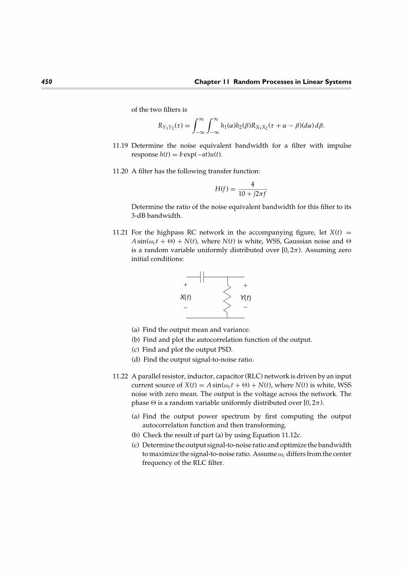
450 Chapter 11 Random Processes in Linear Systems
of the two filters is
RY1Y2 (τ ) =∫ ∞
−∞
∫ ∞
−∞h1(α)h2(β)RX1X2 (τ + α − β)(dα) dβ.
11.19 Determine the noise equivalent bandwidth for a filter with impulseresponse h(t) = b exp(−at)u(t).
11.20 A filter has the following transfer function:
H(f ) = 410 + j2π f
Determine the ratio of the noise equivalent bandwidth for this filter to its3-dB bandwidth.
11.21 For the highpass RC network in the accompanying figure, let X(t) =A sin(ωct + �) + N(t), where N(t) is white, WSS, Gaussian noise and �
is a random variable uniformly distributed over [0, 2π ). Assuming zeroinitial conditions:
X(t ) Y(t )
+
−
+
−
(a) Find the output mean and variance.(b) Find and plot the autocorrelation function of the output.(c) Find and plot the output PSD.(d) Find the output signal-to-noise ratio.
11.22 A parallel resistor, inductor, capacitor (RLC) network is driven by an inputcurrent source of X(t) = A sin(ωct + �) + N(t), where N(t) is white, WSSnoise with zero mean. The output is the voltage across the network. Thephase � is a random variable uniformly distributed over [0, 2π ).
(a) Find the output power spectrum by first computing the outputautocorrelation function and then transforming.
(b) Check the result of part (a) by using Equation 11.12c.(c) Determine the output signal-to-noise ratio and optimize the bandwidth
to maximize the signal-to-noise ratio. Assume ωc differs from the centerfrequency of the RLC filter.

Exercises 451
Hints: You may have to calculate the autocorrelation function as a functionof t and τ and then let t go to infinity to find the steady state output. Thereare several conditions you may want to consider; for example, the filtermay be overdamped, critically damped, or underdamped. It may also havean initial voltage on the capacitor and a current through the inductor. Stateyour assumption about these conditions.
11.23 Suppose you want to learn the characteristics of a certain filter. A whitenoise source with an amplitude of 15 watts/Hz is connected to the input ofthe filter. The power spectrum of the filter output is measured and foundto be
SYY(f ) = 30(2π f )2 + 102 .
(a) What is the bandwidth (3-dB) of the filter?
(b) What is the attenuation (or gain) at zero frequency?
(c) Show one possible (i.e., real, causal) filter that could have producedthis output PSD.
11.24 A one-sided exponential pulse, s(t) = exp(−t)u(t), plus white noise isinput to the finite time integrator of Exercise 11.1. Adjust the width of theintegrator, to, so that the output SNR is maximized at t = to.
11.25
(a) Determine the impulse response of the filter matched to the pulseshape in the accompanying figure. Assume that the filter is designedto maximize the output SNR at time t = 3to.
s (t )
1
−1
tot
3to
(b) Sketch the output of the matched filter designed in part (a) when thesignal s(t) is at the input.
11.26 Find the impulse response and transfer function of a filter matched to atriangular waveform as shown in the accompanying figure when the noiseis stationary and white with a power spectrum of No/2.

452 Chapter 11 Random Processes in Linear Systems
to2
so
s (t )
t
to
11.27 A known deterministic signal, s(t), plus colored (not white) noise, N(t),with a PSD of SNN(f ) is input to a filter. Derive the form of the filter thatmaximizes the SNR at the output of the filter at time t = to. To make thisproblem simpler, you do not need to insist that the filter is causal.
11.28∗ Suppose we observe a random process Z(t) (without any noise) over a timeinterval (−∞, t). Based on this observation, we wish to predict the value ofthe same random process at time t + to. That is, we desire to design a filterwith impulse response, h(t), whose output will be an estimate of Z(t + to):
Y(t) = Z(t + to) =∫ ∞
0h(u)Z(t − u) du.
(a) Find the Wiener-Hopf equation for the optimum (in the minimummean square error (MMSE) sense) filter.
(b) Find the form of the Wiener filter if RZZ(τ ) = exp(−|τ |).(c) Find an expression for the mean square error E[ε2(t)] = E[(Z(t + to) −
Y(t))2].
11.29 (Adapted form Leon-Garcia, 7.49) Suppose we are allowed to observe arandom process Z(t) at two points in time, t0 and t2. Based on these obser-vations we would like to estimate Z(t) at time t = t1 where t0 < t1 < t2.We can view this as an interpolation problem. Let our estimator be a linearcombination of the two observations,
Y(t1) = Z(t1) = aZ(t0) + bZ(t2).
(a) Use the orthogonality principle to find the MMSE estimator.(b) Find an expression for the mean square error of the MMSE estimator.
11.30 (Roughly adapted from Papoulis 14.1 and 14.5) Suppose we are allowedto observe a random process Z(t) at two points in time, t0 and t1. Based on
∗Adapted from Leon-Garcia, 7.59

Exercises 453
those observations, we would like to estimate Z(t) at time t = t2 wheret0 < t1 < t2. We can view this as a prediction problem. Let our estimatorbe a linear combination of the two observations,
Y(t2) = Z(t2) = aZ(t0) + bZ(t1).
(a) Use the orthogonality principle to find the MMSE estimator.
(b) Suppose that RZZ(τ ) = c exp(−b|τ |) for positive constants b and c. Showthat in this case, the sample at time t = t0 is not useful for predictingthe value of the process at time t = t2 (given we have observed theprocess at time t = t1 > t0). In other words, show that a = 0.
11.31 The sum of two independent random processes with power spectraldensities
SSS(f ) = 250 + (2π f )2 and SNN(f ) = 40
are input to an linear time invariant (LTI) filter.
(a) Determine the Wiener smoothing filter. That is, find the impulseresponse of the filter that produces an output that is an MMSE estimateof S(t).
(b) Find the PSD of the filtered signal plus noise.
11.32 The sum of two independent random sequences with autocorrelationfunctions
RSS[k] = 10
1 −(
110
)2
(110
)|k|and RNN[k] = 100
1 −(
14
)2
(14
)|k|
are input to an LTI filter.
(a) Determine the Wiener smoothing filter. That is, find the impulseresponse of the filter that produces an output that is an MMSE estimateof S[n].
(b) Find the PSD of the filtered signal plus noise.
(c) Find the input SNR and an estimate of the output SNR. Discuss whetheror not the Wiener filter improves the SNR.

454 Chapter 11 Random Processes in Linear Systems
Hint: Compare the spectra of the Wiener filter, the signal, and the noise byplotting each on the same graph.
MATLAB Exercises11.33 (a) Construct a signal plus noise random sequence using 10 samples of
X[n] = cos(2π fonts) + N[n],
where N[n] is generated using randn in MATLAB and fo = 0. 1/ts.Design a discrete time matched filter for the cosine signal. Filter thesignal plus noise sequence with the matched filter. At what samplevalue does the filter output peak?
(b) Construct a signal plus noise random sequence using 10 samples of
X[n] = cos(2π f1nts) + 10 cos(2π f2nts) + N[n],
where N[n] is generated using randn in MATLAB, f1 = 0. 1/ts, andf2 = 0. 4/ts. Design a discrete time matched filter for the f2 cosine signal.Filter the signal plus noise sequence with the matched filter. At whatsample value does the filter output peak?
11.34 If a random sequence has an autocorrelation function RXX[k] = 10(0. 8|k|),
find the discrete time, pure prediction Wiener filter. That is, find the filterh[n] such that when X[n] is input, the output, Y[n], will be an MMSEestimate of X[n+1]. Determine and plot the PSD for the random sequenceand the power transfer function, |H(f )|2, of the filter.
11.35 You have a random process with the correlation matrix
1. 0 0. 3 0. 09 0. 0270. 3 1. 0 0. 3 0. 09
0. 09 0. 3 1. 0 0. 30. 027 0. 09 0. 3 1. 0
Determine the pure prediction Wiener filter. That is, find the coefficients ofthe impulse response, h = [h0, h1, h2, 0, 0, 0, . . .]. Then determine the powerspectrum of the Wiener filter. Are the results what you expected?

MATLAB Exercises 455
11.36 Generate a 100-point random sequence using randn(1,100) inMATLAB. Use a first-order autoregressive (AR) filter to filter this randomprocess. That is, the filter is
A(z) = 11 + a1z−1 .
Let a1 = −0. 1. Use the filtered data to obtain an estimate for the first-orderprediction Wiener filter. Compare the estimated filter coefficient with thetrue value.

Simulation Techniques 12
With the increasing computational power of very inexpensive computers, sim-ulation of various systems is becoming very common. Even when a problem isanalytically tractable, sometimes it is easier to write a quick program to simulatethe desired results. However, there is a certain art to building good simulations,and many times avoidable mistakes have led to incorrect simulation results. Thischapter aims at helping the reader to build a basic knowledge of some commontechniques used for simulation purposes. Most of the results presented in thischapter are just applications of material covered in previous chapters, so there isnothing fundamentally new here. Nevertheless, armed with some of the basic sim-ulation principles presented in this chapter, the reader should be able to developsimulation tools with confidence.
12.1 Computer Generationof Random Variables
In this section, we study techniques used to generate random numbers. However,we must start with a disclaimer. Most of the techniques used in practice to gen-erate so-called random numbers will actually generate a completely deterministicsequence of numbers. So, what is actually random about these random number gen-erators? Strictly speaking, nothing! Rather, when we speak of computer-generatedrandom numbers, we are usually creating a sequence of numbers that have certainstatistical properties that make them behave like random numbers, but in fact theyare not really random at all. Such sequences of numbers are more appropriatelyreferred to as pseudorandom numbers.
457

458 Chapter 12 Simulation Techniques
12.1.1 Binary Pseudorandom Number Generators
To start with, suppose we would like to simulate a sequence of independent andidentically distributed (IID) Bernoulli random variables, x1, x2, x3, . . . . One way todo this would be to grab a coin and start flipping it and observe the sequence ofheads and tails, which could then be mapped to a sequence of 1s and 0s. One draw-back to this approach is that it is very time consuming. If our application demandeda sequence of length 1 million, not many of us would have the patience to flip thecoin that many times. Naturally, we seek to assign this task to a computer. So, tosimulate an IID sequence of random variables, essentially we would like to createa computer program that will output a binary sequence with the desired statisticalproperties. For example, in addition to having the various bits in the sequence bestatistically independent, we might also want 0s and 1s to be equally likely.
Consider the binary sequence generated by the linear feedback shift register(LFSR) structure illustrated in Figure 12.1. In that figure, the square boxes repre-sent binary storage elements (i.e., flip-flops) while the adder is modulo-2 (i.e., anexclusive OR gate). Suppose the shift register is initially loaded with the sequence1, 1, 1, 1. It is not difficult to show that the shift register will output the sequence
1, 1, 1, 1, 0, 0, 0, 1, 0, 0, 1, 1, 0, 1, 0, . . . . (12.1)
If the shift register were clocked longer, it would become apparent that the outputsequence would be periodic with a period of 15 bits. While periodicity is not adesirable property for a pseudorandom number generator, if we are interested ingenerating short sequences (of length less than 15 bits), then the periodicity of thissequence generator would not come into play. If we are interested in generatinglonger sequences, we could construct a shift register with more stages so that theperiod of the resulting sequence would be sufficiently long that its periodicitywould not be a concern.
The sequence generated by our LFSR does possess several desirable proper-ties. First, the number of ones and zeros is almost equal (8 ones and 7 zeros is asclose as we can get to “equally likely” with a sequence of length 15). Second, theautocorrelation function of this sequence is nearly equal to that of a truly randombinary IID sequence (again, it is as close as we can possibly get with a sequenceof period 15; see Exercise 12.1). Practically speaking, the sequence output by thiscompletely deterministic device does a pretty good job of mimicking the behaviorof an IID binary sequence. It also has the advantage of being repeatable. That is, ifwe load the shift register with the same initial contents, we can always reproducethe exact same sequence.
It should be noted that not all LFSRs will serve as good pseudorandom numbergenerators. Consider for example the four-stage LFSR in Figure 12.2. This shift

12.1 Computer Generation of Random Variables 459
Output
Figure 12.1 A four-stage, binary linear feedback shift register.
+
Output
+
Figure 12.2 Another four-stage, binary linear feedback shift register.
register is only a slightly modified version of the one in Figure 12.1, yet whenloaded with the sequence 1, 1, 1, 1, this shift register outputs a repeating sequenceof all 1s (i.e., the period of the output sequence is 1). The only difference betweenthe two shift registers is in the placement of the feedback tap connections. Clearly,the placement of these tap connections is crucial in creating a good pseudorandomsequence generator.
A general N-stage LFSR is shown in Figure 12.3. The feedback tap gains, gi,i = 0, 1, 2, . . . , N, are each either 0 or 1. A 1 represents the presence of a tap con-nection, while a 0 represents the absence of a tap connection. It is also understoodthat g0 = gN = 1. That is, there must always be connections at the first and lastposition. A specific LFSR can then be described by the sequence of tap connections.For example, the four stage LFSR in Figure 12.1 can be described by the sequenceof tap connections [g0, g1, g2, g3, g4] = [1, 0, 0, 1, 1]. It is also common to further sim-plify this shorthand description of the LFSR by converting the binary sequenceof tap connections to an octal number. For example, the sequence [1, 0, 0, 1, 1]becomes the octal number 23. Likewise, the LFSR in Figure 12.2 is described by[g0, g1, g2, g3, g4] = [1, 0, 1, 1, 1] → 27.
+
Output
++ + . . .
. . .
g0 g1 g2 gN–2 gN–1 gN
Figure 12.3 A general N-stage, binary linear feedback shift register.

460 Chapter 12 Simulation Techniques
An N-stage LFSR must necessarily generate a periodic sequence of numbers.At any point in time, the N-bit contents of the shift register can take on only oneof 2N possibilities. Given any starting state, the LFSR could at best cycle throughall possible states, but sooner or later must return to its initial state (or some otherstate it has already been in). At that point, the output will then begin to repeatitself. Also, note that if the LFSR ever gets into the all zero state, it will remain inthat state and output a sequence of all zeros from that point on. Hence, to get themaximum period out of a LFSR, we would like the shift register to cycle throughall possible nonzero states exactly once before returning to its initial state. This willproduce a periodic output sequence with a period of 2N − 1. Such a sequence isreferred to as a maximal length linear feedback shift register (MLLFSR) sequence, or anm-sequence, for short.
To study the question of how to connect the feedback taps of an LFSR in orderto produce an m-sequence requires a background in abstract algebra beyond thescope of this book. Instead, we include a short list in Table 12.1 describing a fewfeedback connections, in the octal format described, that will produce m-sequences.This list is not exhaustive in that it does not list all possible feedback connectionsfor a given shift register length that lead to m-sequences.
As mentioned, m-sequences have several desirable properties in that theymimic those properties exhibited by truly random IID binary sequences. Someof the properties of m-sequences generated by an N-stage LFSR are summarizedas follows:
• m-sequences are periodic with a period of 2N − 1.• In one period, an m-sequence contains 2N/2 ones and 2N/2 − 1 zeros. Hence,
zeros and ones are almost equally likely.• The autocorrelation function of m-sequences is almost identical to that of an
IID sequence.• Define a run of length n to be a sequence of either n consecutive ones or n
consecutive zeros. An m-sequence will have one run of length N, one run of
Table 12.1 LFSR Feedback Connections for m-sequences
SR length, N Feedback connections (in octal format)
2 73 134 235 45, 75, 676 103, 147, 1557 211, 217, 235, 367, 277, 325, 203, 313, 3458 435, 551, 747, 453, 545, 537, 703, 543

12.1 Computer Generation of Random Variables 461
Output
+
Figure 12.4 A five-stage LFSR with 45 (octal) feedback tap connections.
length N − 1, two runs of length N − 2, four runs of length N − 3, eight runs oflength N − 4, . . . , and 2N−2 runs of length 1.
M-sequences possess many other interesting properties that are not as relevant totheir use as random number generators.
EXAMPLE 12.1: Suppose we wish to construct an m-sequence oflength 31. Since the period of an m-sequence is 2N − 1, we will needan N = 5 stage shift register to do the job. From Table 12.1, there arethree different feedback connections listed, any of which will work.Using the first entry in the table, the octal number 45 translates to thefeedback tap connections (1,0,0,1,0,1). This describes the LFSR shown inFigure 12.4. Assuming this LFSR is initially loaded with the sequence(1,0,0,0,0), the resulting m-sequence will be
(0 0 0 0 1 0 0 1 0 1 1 0 0 1 1 1 1 1 0 0 0 1 1 0 1 1 1 0 1 0 1).
12.1.2 Nonbinary Pseudorandom Number Generators
Next suppose that it is desired to generate a sequence of pseudorandom num-bers drawn from a nonbinary alphabet. One simple way to do this is to modifythe output of the binary LFSRs discussed previously. For example, suppose wewant a pseudorandom number generator that produces octal numbers (i.e, froman alphabet of size 8) that simulates a sequence of IID octal random variables wherethe eight possible outcomes are equally probable. One possible approach would beto take the 5-stage LFSR of Example 12.1, group the output bits in triplets (i.e., threeat a time), and then convert each triplet to an octal number. Doing so (assumingthe LFSR is loaded initially as in Example 12.1), one period of the resulting octalsequence is
(0 2 2 6 3 7 0 6 7 2 4 1 1 3 1 7 4 3 3 5 2 0 4 5 4 7 6 1 5 6 5). (12.2)

462 Chapter 12 Simulation Techniques
Note that each of the octal numbers 0, 1, 2, . . . , 7 occurs exactly four times in thissequence except the number 0, which occurs three times. This is as close as we canget to equally likely octal numbers with a sequence of length 31. The number ofruns of various lengths in this sequence also matches what we might expect froma truly random IID sequence of equally likely octal numbers. For example, theprobability of a run of length 2 occurring in a random sequence of octal numbersis 1/8. Given a random sequence of length 31, the expected number of runs oflength 2 is 31/8 = 3. 875. This pseudorandom sequence has three runs of length 2.The expected number of runs of length 3 is 31/64 = 0. 4844. The pseudorandomsequence has no runs of length 3.
It should be noted that since the octal sequence in Equation 12.2 is generatedby the underlying feedback structure of Example 12.1, there should be a recursiveformula that can be used to generate the sequence. In this case, the recursion isfairly complicated and not very instructive, but this leads us to the idea of gen-erating pseudorandom sequences of nonbinary numbers using some recursiveformula. One commonly used technique is the power residue method whereby apseudorandom sequence is generated through a recursion of the form
xk = axk−1 mod q, k = 1, 2, 3, . . . , (12.3)
where a and q are suitably chosen constants. Due to the modulo-q operation, theelements of the sequence are from the set {0, 1, 2, . . . , q − 1}. The first element of thesequence x0 is called the seed and given the set {a, q, x0}, the resulting sequence iscompletely deterministic. Note also that the resulting sequence must be periodicsince once any element appears a second time in the sequence, the sequence willthen repeat itself. Furthermore, since the elements of the sequence are from a finitealphabet with q symbols, the maximum period of the sequence is q − 1 (the periodis not q because the element 0 must never appear or the sequence will produce all0s after that and hence be of period 1). The next example shows that the desirablestatistical properties of the sequence are dependent upon a careful selection of thenumbers a and q.
EXAMPLE 12.2: First suppose that {a, q} = {4, 7}. Then the sequenceproduced has a period of 3 and assuming that the seed is x0 = 1, thesequence is given by
(x0, x1, x2, . . .) = (1, 4, 2, 1, 4, 2, 1, 4, 2, . . .).
This is not a particularly good result since with the selection of q = 7,we would hope for a period of q − 1 = 6. However, if we make a slight

12.1 Computer Generation of Random Variables 463
change so that {a, q} = {3, 7}, with the seed of x0 = 1, the sequencebecomes
(x0, x1, x2, . . .) = (1, 3, 2, 6, 4, 5, 1, 3, 2, 6, 4, 5, . . .).
Now, as desired, the sequence has the maximal period of 6 and cyclesthrough each of the integers from 1 through 6 exactly once each. Asanother example of a choice of {a, q} that leads to a bad sequence, sup-pose we selected {a, q} = {4, 8}. Then the sequence produced (assumingx0 = 1) would be
(x0, x1, x2, . . .) = (1, 4, 0, 0, 0, . . .).
Clearly, we can get pseudorandom sequences with very different statisticalproperties depending on how we choose {a, q}. By choosing the number q to be verylarge, the resulting period of the pseudorandom sequence will also be very large,and hence the periodicity of the sequence will not become an issue. Most mathpackages and high-level programming languages have built in random numbergenerators that use this method. Commonly, the parameters {a, q} = {75, 231 − 1}are used. This produces a sequence of length 231 − 2, which is over 2 billion.Furthermore, by normalizing the elements of the sequence by q, the resulting pseu-dorandom sequence has elements from the set {1/q, 2/q, . . . , (q−1)/q}. With a verylarge choice for the value of q, for almost all practical purposes, the elements willappear to be drawn from the continuous interval (0, 1). Hence, we have constructeda simple method to simulate random variables drawn from a uniform distribution.
12.1.3 Generation of Random Numbers from aSpecified Distribution
Quite often we are interested in generating random variables that obey some distri-bution other than a uniform distribution. In this case, it is generally a fairly simpletask to transform a uniform random number generator into one that follows someother distribution. Consider forming a monotonic increasing transformation g()on a random variable X to form a new random variable Y. From the results ofChapter 4, the PDFs of the random variables involved are related by
fY(y) = fX(x)dg(x)/dx
. (12.4)
Given an arbitrary PDF, fX(x), the transformation Y = g(X) will produce a uniformrandom variable Y if dg/dx = fX(x), or equivalently g(x) = FX(x). Viewing this

464 Chapter 12 Simulation Techniques
result in reverse, if X is uniformly distributed over (0, 1) and we want to create anew random variable, Y, with a specified distribution, FY(y), the transformationY = F−1
Y (X) will do the job.
EXAMPLE 12.3: Suppose we want to transform a uniform randomvariable into an exponential random variable with a PDF of the form
fY(y) = a exp(−ay)u(y).
The corresponding CDF is
FY(y) = [1 − exp(−ay)]u(y).
Hence, to transform a uniform random variable into an exponentialrandom variable, we can use the transformation
Y = F−1Y = − ln(1 − X)
a.
Note that if X is uniformly distributed over (0, 1), then 1 − X will beuniformly distributed as well so that the slightly simpler transformation
Y = − ln(X)a
will also work.
This approach for generation of random variables works well provided thatthe CDF of the desired distribution is invertible. One notable exception where thisapproach will be difficult is the Gaussian random variable. Suppose, for example,we wanted to transform a uniform random variable, X, into a standard normalrandom variable, Y. The CDF in this case is the complement of a Q-function,FY(y) = 1 − Q(y). The inverse of this function would then provide the appro-priate transformation, y = Q−1(1 − x), or as with the previous example, we couldsimplify this to y = Q−1(x). The problem here lies with the inverse Q-function,which cannot be expressed in a closed form. One could devise efficient numeri-cal routines to compute the inverse Q-function, but fortunately there is an easierapproach.
An efficient method to generate Gaussian random variables from uniform ran-dom variables is based on the following 2×2 transformation. Let X1 and X2 be twoindependent uniform random variables (over the interval (0,1)). Then if two new
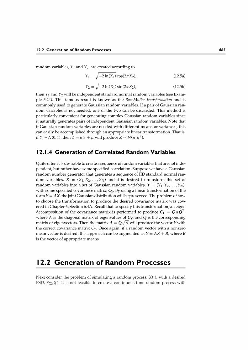
12.2 Generation of Random Processes 465
random variables, Y1 and Y2, are created according to
Y1 =√
−2 ln(X1) cos(2πX2), (12.5a)
Y2 =√
−2 ln(X1) sin(2πX2), (12.5b)
then Y1 and Y2 will be independent standard normal random variables (see Exam-ple 5.24). This famous result is known as the Box-Muller transformation and iscommonly used to generate Gaussian random variables. If a pair of Gaussian ran-dom variables is not needed, one of the two can be discarded. This method isparticularly convenient for generating complex Gaussian random variables sinceit naturally generates pairs of independent Gaussian random variables. Note thatif Gaussian random variables are needed with different means or variances, thiscan easily be accomplished through an appropriate linear transformation. That is,if Y ∼ N(0, 1), then Z = σY + µ will produce Z ∼ N(µ, σ 2).
12.1.4 Generation of Correlated Random Variables
Quite often it is desirable to create a sequence of random variables that are not inde-pendent, but rather have some specified correlation. Suppose we have a Gaussianrandom number generator that generates a sequence of IID standard normal ran-dom variables, X = (X1, X2, . . . , XN) and it is desired to transform this set ofrandom variables into a set of Gaussian random variables, Y = (Y1, Y2, . . . , YN),with some specified covariance matrix, CY. By using a linear transformation of theform Y = AX, the joint Gaussian distribution will be preserved. The problem of howto choose the transformation to produce the desired covariance matrix was cov-ered in Chapter 6, Section 6.4A. Recall that to specify this transformation, an eigendecomposition of the covariance matrix is performed to produce CY = Q�QT ,where � is the diagonal matrix of eigenvalues of CY, and Q is the correspondingmatrix of eigenvectors. Then the matrix A = Q
√� will produce the vector Y with
the correct covariance matrix CY. Once again, if a random vector with a nonzeromean vector is desired, this approach can be augmented as Y = AX + B, where Bis the vector of appropriate means.
12.2 Generation of Random Processes
Next consider the problem of simulating a random process, X(t), with a desiredPSD, SXX(f ). It is not feasible to create a continuous time random process with

466 Chapter 12 Simulation Techniques
a computer. Fortunately, we can invoke the sampling theorem to represent thecontinuous time random process by its samples. Let Xk = X(kTs) be the kth sampleof the random process taken at a sampling rate of Rs = 1/Ts. Then, provided thesampling rate is chosen to be at least twice the absolute bandwidth of X(t) (i.e., twicethe largest nonzero frequency component of SXX(f )), the random process can bereproduced from its samples. Thus, the problem of generating a random processcan be translated into one of creating a sequence of random variables. The questionis how should the random variables be correlated in order to produce the correctPSD? Of course, the autocorrelation function, RXX(τ ), provides the answer to thisquestion. If the random process is sampled at a rate of Rs = 1/Ts, then the kth andmth sample will have a correlation specified by E[XkXm] = RXX((k − m)Ts). Hence,if X = (X1, X2, . . . , XN) is a sequence of samples of the random process X(t), thecorrelation matrix of these samples will have a Toeplitz structure (assuming X(t)is stationary) of the form
RXX =
RXX(0) RXX(Ts) RXX(2Ts) . . . RXX(NTs)RXX(−Ts) RXX(0) RXX(Ts) . . . RXX((N−1)Ts)
RXX(−2Ts) RXX(−Ts) RXX(0) . . . RXX((N−2)Ts). . . . . . . . . . . .
RXX(−NTs) RXX(−(N−1)Ts) RXX(−(N−2)Ts) . . . RXX(0)
.
(12.6)
Once the appropriate correlation matrix is specified, the procedure developed inthe last section can be used to generate the samples with the appropriate correlationmatrix.
This approach will work fine provided that the number of samples desired is nottoo large. However, in many cases, we need to simulate a random process for a largetime duration. In that case, the number of samples, N, needed becomes large andhence the matrix RXX is also large. Performing the necessary eigendecompositionon this matrix then becomes a computationally intensive problem. The followingsections look at some alternative approaches to this general problem that offer somecomputational advantages.
12.2.1 Frequency Domain Approach
If the random process to be simulated is a Gaussian random process, we canapproach the problem by creating samples of the random process in the frequencydomain. Suppose we wish to create a realization of the random process, X(t), oftime duration Td, say over the interval (0, Td), and that we don’t much care whathappens to the process outside this interval. To start with, we produce a periodic

12.2 Generation of Random Processes 467
X(t)
Td
X~
(t)
Td 2Td 3Td
Figure 12.5 A realization of the random process X(t) along with its periodic extension X(t).
signal X(t) by repeating X(t) every Td seconds as illustrated in Figure 12.5. SinceX(t) is periodic, it has a Fourier series representation
X(t) =∑
k
Xke j2πkfot, fo = 1Td
. (12.7)
Note that due to the linearity of the Fourier series construction, if the Xk are zero-mean Gaussian random variables, then the resulting process X(t) will be a zero-mean Gaussian random process. Furthermore, the periodic random process X(t)has a line spectrum given by
SX, X(f ) =∑
k
s2kδ(f − kfo), s2
k = E[∣∣Xk
∣∣2]
. (12.8)
The sk can be chosen to shape the spectrum to any desired form. If the desired PSDof the random process is SXX(f ), then we could pick s2
k ∝ Sxx(kfo). The constant ofproportionality can be chosen so that the total power in the process X(t) matchesthat of X(t). In particular, suppose that X(t) is bandlimited so that SXX(f ) = 0for |f | > W . Then the number of terms in the Fourier series in Equation 12.7 isfinite. Let
M =⌊
Wfo
⌋= �WTd�. (12.9)
Then sk will be nonzero only for |k| ≤ M. Hence, we need to generate a total of2M + 1 random variables, X−M , X−M+1, . . . , X−1, X0, X1, . . . , XM . The variances ofthese random variables are chosen such that
s2k = E
[∣∣Xk∣∣2
]= βSXX(kfo), β =
∫ W
−WSXX(f ) df
∑Mk=−M SXX(kfo)
. (12.10)

468 Chapter 12 Simulation Techniques
In summary, the random process can be simulated by first generating a sequenceof 2M + 1 zero-mean complex Gaussian random variables. Each random variableshould be scaled so that the variances are as specified in Equation 12.10. Samplesof the random process in the time domain can be constructed for any desired timeresolution, �t, according to
X[i] = X(i�t) =M∑
k=−M
Xk(e j2π fo�t)ik. (12.11)
If the random process is real, it is sufficient to generate the M + 1 random vari-ables X0, X1, . . . , XM independently and then form the remaining random variablesX−1, X−2, . . . , X−M using the conjugate symmetry relationship X−k = X∗
k . In thiscase, X0 must also be real so that a total 2M +1 real Gaussian random variables areneeded (one for X0 and two each for Xk, k = 1, 2, . . . , M) to construct the randomprocess, X(t).
EXAMPLE 12.4: Suppose we wish to generate a 5-msec segmentof a real zero-mean Gaussian random process with a PSD given by
SXX(f ) = 11 + (f /f3)4 ,
where f3 = 1 kHz is the 3-dB frequency of the PSD. Strictly speaking, thisprocess has an infinite absolute bandwidth. However, for sufficiently highfrequencies there is minimal power present. For the purposes of this exam-ple, we (somewhat arbitrarily) take the bandwidth to be W = 6f3 so thatapproximately 99.9 percent of the total power in the process is containedwithin |f | < W . Since we want to simulate a time duration of Td = 5 msec,the number of Fourier series coefficients needed is given by M = �WTd� = 30.Figure 12.6 shows a comparison of the actual PSD, SXX(f ), with the discreteline spectrum approximation. Also, one realization of the random processgenerated by this method is shown in Figure 12.7. The MATLAB code usedto create these plots follows.
% Set parameters.
I=sqrt(-1);
Td=5e-3; fo=1/Td; f3=1e3; dt=1e-5;
M=floor(6*f3*Td); m=[-M:M];
% Construct discrete samples of PSD.
x=[0:0.01:10]; psd=1./(1+x.∧4);
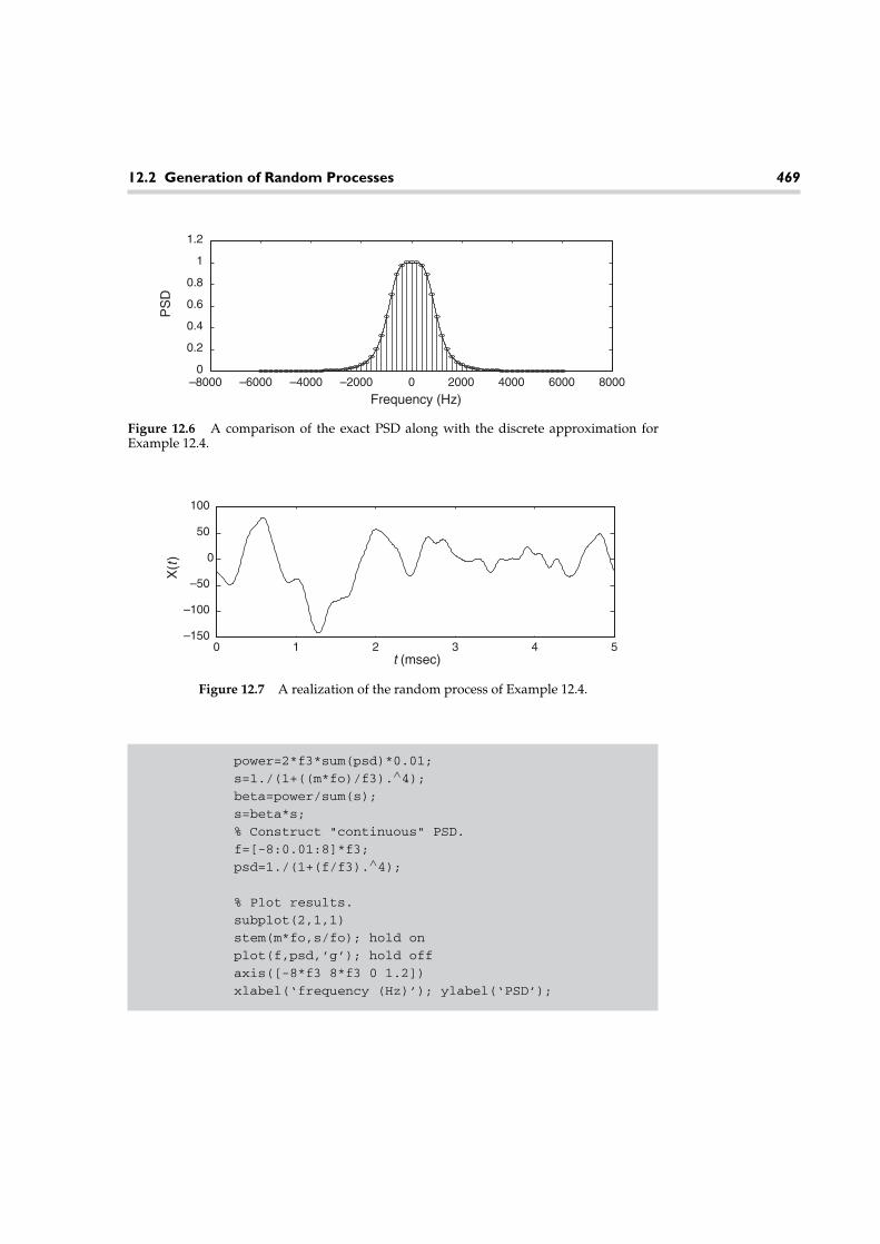
12.2 Generation of Random Processes 469
–8000 –6000 –4000 –2000 0 2000 4000 6000 80000
0.2
0.4
0.6
0.8
1
1.2
Frequency (Hz)
PS
D
Figure 12.6 A comparison of the exact PSD along with the discrete approximation forExample 12.4.
0 1 2 3 4 5–150
–100
–50
0
50
100
t (msec)
X(t
)
Figure 12.7 A realization of the random process of Example 12.4.
power=2*f3*sum(psd)*0.01;
s=1./(1+((m*fo)/f3).∧4);beta=power/sum(s);
s=beta*s;
% Construct "continuous" PSD.
f=[-8:0.01:8]*f3;
psd=1./(1+(f/f3).∧4);
% Plot results.
subplot(2,1,1)
stem(m*fo,s/fo); hold on
plot(f,psd,’g’); hold off
axis([-8*f3 8*f3 0 1.2])
xlabel(‘frequency (Hz)’); ylabel(‘PSD’);
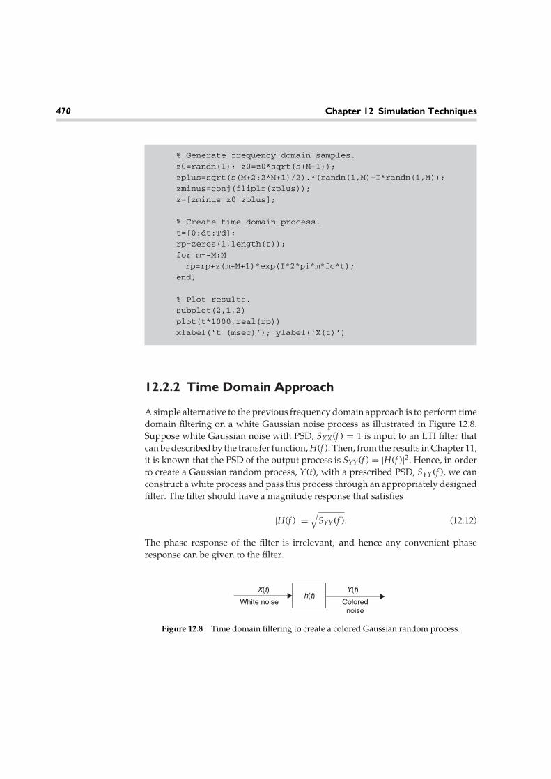
470 Chapter 12 Simulation Techniques
% Generate frequency domain samples.
z0=randn(1); z0=z0*sqrt(s(M+1));
zplus=sqrt(s(M+2:2*M+1)/2).*(randn(1,M)+I*randn(1,M));
zminus=conj(fliplr(zplus));
z=[zminus z0 zplus];
% Create time domain process.
t=[0:dt:Td];
rp=zeros(1,length(t));
for m=-M:M
rp=rp+z(m+M+1)*exp(I*2*pi*m*fo*t);
end;
% Plot results.
subplot(2,1,2)
plot(t*1000,real(rp))
xlabel(‘t (msec)’); ylabel(‘X(t)’)
12.2.2 Time Domain Approach
A simple alternative to the previous frequency domain approach is to perform timedomain filtering on a white Gaussian noise process as illustrated in Figure 12.8.Suppose white Gaussian noise with PSD, SXX(f ) = 1 is input to an LTI filter thatcan be described by the transfer function, H(f ). Then, from the results in Chapter 11,it is known that the PSD of the output process is SYY(f ) = |H(f )|2. Hence, in orderto create a Gaussian random process, Y(t), with a prescribed PSD, SYY(f ), we canconstruct a white process and pass this process through an appropriately designedfilter. The filter should have a magnitude response that satisfies
|H(f )| =√
SYY(f ). (12.12)
The phase response of the filter is irrelevant, and hence any convenient phaseresponse can be given to the filter.
White noise Colorednoise
X(t) Y(t)h(t)
Figure 12.8 Time domain filtering to create a colored Gaussian random process.

12.2 Generation of Random Processes 471
This technique is particularly convenient when the prescribed PSD, SYY(f ) canbe written as the ratio of two polynomials in f . Then the appropriate transferfunction can be found through spectral factorization techniques. If the desiredPSD is a more complicated function of f , then designing and/or implementing afilter to produce that PSD may be difficult. In that case, it may be necessary to usean approximate filter design.
EXAMPLE 12.5: In this example, we design the filter needed to generatethe random process specified in Example 12.4 using the time domainmethod. The PSD is factored as follows:
S(f )= 11+(f /f3)4 = f 4
3(f −f3e jπ/4
)(f −f3e j3π/4
)(f −f3e j5π/4
)(f −f3e j7π/4
) .
If the first two poles are associated with H(f ) (and the last two withH∗(f )), then the filter has a transfer function of
H(f ) = f 23(
f − f3e jπ/4)(
f − f3e j3π/4) = f 2
3
f 2 − j√
2f3f − f 23
,
which can be represented in the time domain as
h(t) = −2ωoe−ωot sin(ωot)u(t),
where ωo = √2π f3. For the purposes of creating a random process with
the desired spectrum, the negative sign in front of this impulse responseis irrelevant and can be ignored. Hence, to produce the desired randomprocess, we start by generating a white Gaussian random process andthen convolve the input with the impulse response specified.
Once an appropriate analog filter has been designed, the filter must be convertedto a discrete time form. If the sampling rate is taken to be sufficiently high, thenthe impulse response of the discrete time filter can be found by simply samplingthe impulse response of the continuous time filter. This is the so-called impulseinvariance transformation. However, because of aliasing that occurs in the processof sampling the impulse response, the frequency response of the digital filter willnot be identical to that of the original analog filter unless the analog filter is abso-lutely bandlimited. Of course, if the analog filter is approximately bandlimited andif the sampling rate is sufficiently large, this aliasing can be kept to a minimum andthe resulting digital filter will produce a very good approximation to the desiredfrequency response.

472 Chapter 12 Simulation Techniques
An alternative popular approach for producing a digital filter from an analogdesign is to use a bilinear transformation. That is, suppose we have an analog filterwith transfer function Ha(s), a digital approximation to this filter, Hd(z), can beobtained (assuming a sampling frequency of fs) according to
Hd(z) = Ha(s)∣∣s=2fs
(1−z−1
1+z−1
). (12.13)
One advantage of the bilinear transformation is that if the analog filter is stable,then the digital filter will be stable as well. Note also that if the analog filter is annth-order filter, then the order of the digital filter will be no more than n as well.
EXAMPLE 12.6: In this example, we find the digital approxima-tion to the analog filter designed in Example 12.5 using the bilinearapproximation. From the results of that example, the analog filterwas a second-order Butterworth filter whose transfer function (in
terms of s) was given by
Ha(s) = ω23
s2 + √2ω3s + ω2
3
,
where ω3 = 2π f3 is the 3-dB frequency of the filter in radians per second. Aftera little bit of algebraic manipulation, application of the bilinear transformationin Equation 12.13 results in
Hd(z) = b0 + b1z−1 + b2z−2
a0 + a1z−1 + a2z−2 ,
where b0 = 1, b1 = 2, b2 = 1, a0 = 1 + √2γ + γ 2, a1 = 2 − 2γ 2, a2 =
1 − √2γ + γ 2, and γ = fs/(π f3). Figure 12.9 shows a plot of the impulse
response of this filter as well as one realization of the random process createdby passing white Gaussian noise through this filter. Note that for this example,the impulse response of the filter lasts for about 1 msec (this makes sense sincethe bandwidth was 1 kHz). Therefore, when creating the filtered process, atleast the first millisecond of output data should be discarded since the contentsof the digital filter have not reached a statistical steady state until that point.The relevant MATLAB code follows.
I=sqrt(-1);
imp_len=150; % Length of impulse response in samples.
sim_len=150; % Length of simulation in samples.

12.2 Generation of Random Processes 473
0 0.5 1 1.5 2 2.5 3 3.5 4 4.5 5–0.02
0
0.02
0.04
0.06
0.08
0.1
Time (msec) = n/fs
h[n]
0 0.5 1 1.5 2 2.5 3 3.5 4 4.5 5–0.4
–0.2
0
0.2
0.4
0.6
Time (msec)
X(t
)
(a)
(b)
Figure 12.9 Impulse response and a single realization of the output of the filter designedin Example 12.6.
f3=1000; % 3-dB frequency of desired PSD.
fs=30000; % Sampling rate.
g=fs/(pi*f3); % Compute filter coefficients.
b0=1; b1=2; b2=1; b=[b0 b1 b2];
a0=1+sqrt(2)*g+g∧2; a1=2-2*g∧2;a2=1-sqrt(2)*g+g∧2; a=[a0 a1 a2];
x=zeros(1,imp_len); x(1)=1; % Impulse.
y=filter(b,a,x); % Impulse response of filter.
time_scale=[1:length(y)]/fs;
subplot(2,1,1) % Plot impulse response.
stem(time_scale*1000,y,‘o’)
xlabel(‘time(msec)=n/f_s’)
ylabel(‘h[n]’)
x=randn(1,sim_len); % White Gaussian random process.
y=filter(b,a,x); % Filtered process.
time_scale=[1:length(y)]/fs;
subplot(2,1,2) % Plot realization.
plot(time_scale*1000,y);
xlabel(‘time (msec)’); ylabel(‘X(t)’);

474 Chapter 12 Simulation Techniques
One advantage of the time domain approach is that it is convenient for gener-ating very long realizations of the random process. Once the filter is designed, theoutput process is created by performing a convolution of the impulse response ofthe filter with a white input sequence. The complexity of this operation is linear inthe length of the sequence. However, the process of creating a long sequence canbe broken into several smaller sequences. The smaller sequences can then be con-catenated together to create a long sequence. There will be no discontinuities at thepoints of concatenation if the contents of the filter are stored after each realizationand used as the starting contents for the next realization.
Some care must be taken when using the time domain method if the desiredsampling rate of the process is much larger than the bandwidth of the filter. In thiscase, the poles of the digital filter will be close to the unit circle and the filter mightexhibit stability problems. This is illustrated in Figure 12.10, where the magnitudeof the poles of the digital filter from Example 12.6 are plotted as a function of thesampling rate. Note that when the rate at which the process is sampled becomes afew hundred times the bandwidth of the filter, the poles of the digital filter becomevery close to the unit circle. This problem can be easily avoided by creating a digitalfilter to create samples of the process at a lower rate (perhaps at several times the
103 104 105 106 1070.4
0.5
0.6
0.7
0.8
0.9
1
fs (Hz)
zp
Figure 12.10 Magnitude of the filter poles as a function of sampling frequency for thefilter designed in Example 12.6.

12.2 Generation of Random Processes 475
bandwidth of the filter so as to avoid aliasing) and then upsampling (throughinterpolation) the resulting process to any desired rate.
12.2.3 Generation of Gaussian White Noise
Generation of a white noise process is exceedingly common and also very simple.However, it is often the source of frequent mistakes among engineers, so we feltit worth making a few comments about computer generation of white Gaussiannoise processes. The source of confusion in the generation of white noise is thatone cannot represent white noise from its time domain samples. White noise hasinfinite power, therefore samples of a white noise process would require infinitevariance. Alternatively, white noise has infinite bandwidth, so the Nyquist rate forrecovering white noise from its samples would be infinite. In order to represent a“white” process in discrete time, we must invoke some form of prefiltering beforesampling. This will limit the bandwidth such that a finite sampling rate can be used,and at the same time it will limit the power of the process such that the resultingsamples of the filtered white process will have a finite variance.
Strictly speaking, once we filter the white noise it is no longer white, but thisshould not be of too much concern. In practice, there is no such thing as trulywhite noise. Recall that the white noise model was an approximation to a noiseprocess that had a constant PSD over a very large (but not infinite) bandwidth.Any equipment we use to measure or receive the noise will automatically filterthe process. With this in mind, we imagine a prefilter that has a bandwidth muchlarger than any bandwidth we are concerned with in the specific system we aresimulating. The noise we create, although not truly white, will behave as thoughit were white for all practical purposes.
In order to simplify the process of creating the samples of the prefiltered whitenoise, it is common to employ an ideal lowpass prefilter with bandwidth W asillustrated in Figure 12.11. Now that the process is bandlimited, it can be repre-sented by samples at any rate that satisfies fs ≥ 2W . Since the prefilter is ideal, theautocorrelation function of the filter output is easily calculated to be
R(τ ) = NoW sinc(2W τ ). (12.14)
Ideal LPFBW=W
Samplerrate= fs
Whitenoise
PSD=No/2
Discrete timenoise process
Figure 12.11 A/D conversion process for white noise.

476 Chapter 12 Simulation Techniques
Note that since this sinc function has nulls at multiples of 1/2W , the samplesof the filtered process will be uncorrelated provided that the samples are spacedby any integer multiple of 1/2W . In other words, if the sampling rate satisfiesfs = 2W /n for any integer n, then the samples of the prefiltered white noise will beuncorrelated. By choosing n = 1 so that the sampling rate is exactly the Nyquist rate,fs = 2W , the process can be recovered from the discrete samples and the samplesare uncorrelated. For Gaussian noise, this implies that the filtered white noise can berepresented by a sequence of independent, zero-mean, Gaussian random variableswith variance of σ 2 = NoW . Note that the variance of the samples and the rate atwhich they are taken are related by σ 2 = Nofs/2.
The lesson to be learned here is that if we wish to represent Gaussian white noiseas a sequence of independent Gaussian random variables, then there is an implicitassumption about the nature of the prefiltering. Furthermore, to be consistent withthis assumption, the variance of the samples must be adjusted when the samplingrate is changed. The variance and sampling rate cannot be selected independently.
12.3 Simulation of Rare Events
Quite often, we are interested in estimating the probability of some event, A. If ana-lytically calculating this probability is too cumbersome, we can design a computerprogram to simulate the system in question and then observe whether or not theevent occurs. By repeating this procedure many times, we can observe how oftenthe event A occurs, and hence get an estimate of its probability through a relativefrequency approach. The event A could be a bit error in a digital communicationssystem—in which case we are interested in calculating bit error probability—or itcould be a buffer overflow in a computer network or even something as extravagantas breaking the bank at the blackjack table.
12.3.1 Monte Carlo Simulations
In general, suppose we have the ability to recreate (simulate) the experiment anarbitrary number of times and define a sequence of Bernoulli random variables,Xi, that are defined according to
Xi ={
1 if A occurs during the ith experiment
0 otherwise. (12.15)

12.3 Simulation of Rare Events 477
Hence, Xi is simply an indicator function for the event A. If the experiments areindependent, then the probability of the event A, pA, can be estimated according to
pA = 1n
n∑i=1
Xi. (12.16)
This is nothing more than estimating the mean of an IID sequence of randomvariables. From the development of Chapter 7, we know that this estimator isunbiased and that as n → ∞ the estimate converges (almost everywhere via thestrong law of large numbers) to the true probability.
In practice, we do not have the patience to run our simulation an infinite numberof times nor do we need to. At some point the accuracy of our estimate should be“good enough,” but how many trials is enough? Some very concrete answers tothis question can be obtained using the theory developed in Chapter 7. If the eventA is fairly probable, then it will not take too many trials to get a good estimate ofthe probability, in which case runtime of the simulation is not really too much ofan issue. However, if the event A is rare, then we will need to run many trials toget a good estimate of pA. In the case where n gets large, we want to be sure notto make it any larger than necessary so that our simulation runtimes do not getexcessive. Thus, the question of how many trials to run becomes important whensimulating rare events.
Assuming n is large, the random variable pA can be approximated as a Gaussianrandom variable via the central limit theorem. The mean and variance are E[pA] =pA and σ 2
pA= n−1pA(1−pA), respectively. One can then set up a confidence interval
based on the desired accuracy. For example, suppose we wish to obtain an estimatethat is within 1 percent of the true value with 90 percent probability. That is, wewant to run enough trials to insure that
Pr(∣∣pA − pA
∣∣ < 0. 01pA) = 0. 9 = 1 − α (12.17)
From the results of Chapter 7, Section 7.5, we get
ε0.1 = 0. 01pA = σX√n
c0.1 =√
pA(1 − pA)n
c0.1, (12.18)
where the value of c0.1 is taken from Table 7.1 as c0.1 = 1. 64. Solving for n gives usan answer for how long to run the simulation:
n = (100c0.1)2(1 − pA)pA
= (164)2(1 − pA)pA
≈ (164)2
pA. (12.19)
Or in general, if we want the estimate, pA, to be within β percent of the true value(i.e.,
∣∣pA − pA∣∣ < βpA/100) with probability 1 − α, then the number of trials in the

478 Chapter 12 Simulation Techniques
simulation should be chosen according to
n =
(100cα
β
)2
(1 − pA)
pA≈
(100cα
β
)2
pA. (12.20)
This result is somewhat unfortunate because in order to know how long to run thesimulation, we have to know the value of the probability we’re trying to estimate inthe first place. In practice, we may have a crude idea of what to expect for pA, whichwe could then use to guide us in selecting the number of trials in the simulation.However, we can use this result to give us very specific guidance in how to choosethe number of trials to run, even when pA is completely unknown to us. Definethe random variable NA to be the number of occurrences of the event A in n trials;that is,
NA =n∑
i=1
Xi. (12.21)
Note that E[NA] = npA. That is, the quantity npA can be interpreted as theexpected number of occurrences of the event A in n trials. Multiplying both sidesof Equation 12.20 by pA then produces
E[NA] =(
100cα
β
)2
(1 − pA) ≈(
100cα
β
)2
. (12.22)
Hence, one possible procedure to determine how many trials to run is to repeatthe experiment for a random number of trials until the event A occurs some fixednumber of times as specified by Equation 12.22. Let Mk be the random variable thatrepresents the trial number of the kth occurrence of the event A. Then, one couldform an estimate of pA according to
pA = kMk
. (12.23)
It turns out that this produces a biased estimate; however a slightly modified form,
pA = k − 1Mk − 1
, (12.24)
produces an unbiased estimate (see Exercise 7.12).
EXAMPLE 12.7: Suppose we wish to estimate the probability of anevent that we expect to be roughly on the order of p ∼ 10−4.

12.3 Simulation of Rare Events 479
Assuming we want 1 percent accuracy with a 90 percent confidencelevel, the number of trials needed will be
n = 1p
(100cα
β
)2
= 104(
100 ∗ 1. 641
)2
= 268, 960, 000.
Alternatively, we need to repeat the simulation experiment until weobserve the event
NA =(
100cα
β
)2
= 26, 896 times.
Assuming we do not have enough time available to repeat our simula-tion over 1/4 of a billion times, we would have to accept less accuracy.Suppose that due to time limitations we decide that we can only repeatour experiment 1 million times, then we can be sure that with 90 percentconfidence, the estimate will be within the interval (p − ε, p + ε), if ε ischosen according to
ε =√
p(1 − p)√n
cα ≈√
p√n
cα = 1. 6410−2
103 = 1. 64 × 10−5 = 0. 164p.
With one million trials, we can only be 90 percent sure that the estimateis within 16.4 percent of the true value.
The preceding example demonstrates that using the Monte Carlo approachto simulating rare events can be very time consuming in that we may need torepeat our simulation experiments many times to get a high degree of accuracy.If our simulations are complicated, this may put a serious strain on our computa-tional resources. The next section presents a novel technique, which when appliedintelligently can substantially reduce the number of trials we may need to run.
12.3.2 Importance Sampling
The general idea behind importance sampling is fairly simple. In the Monte Carloapproach, we spend a large amount of time with many repetitions of an experimentwhile we are waiting for an event to occur that may happen only very rarely. Inimportance sampling, we skew the distribution of the underlying randomness inour experiment so that the “important” events happen more frequently. We canthen use analytical tools to convert our distorted simulation results into an unbiasedestimate of the probability of the event in which we are interested. To help present
480 Chapter 12 Simulation Techniques
this technique, we first generalize the problem treated in Section 12.3.1. Supposethe simulation experiment consisted of creating a sequence of random variables,X = (X1, X2, . . . , Xm) according to some density, fX(x), and then observing whetheror not some event A occurred which could be defined in terms of the Xi. Forexample, suppose Xi represents the number of messages that arrive at a certain nodein a computer communications network at time instant i. Furthermore, supposethat it is known that the node requires a fixed amount of time to forward eachmessage along to its intended destination and that the node has some finite buffercapacity for storing messages. The event A might represent the event that the node’sbuffer overflows, and hence a message is lost during the time interval i = 1, 2, . . . , m.Ideally, the communications network has been designed so that this event is fairlyuncommon, but it is desirable to quantify how often this overflow will occur. Whileit may be fairly straightforward to determine whether or not a buffer overflow hasoccurred given a specific sequence of arrivals, X = x, determining analytically theprobability of buffer overflow may be difficult, so we decide to approach this viasimulation. Let ηA(X) be an indicator function for the event A. That is, let ηA(x) = 1if x is such that the event A occurs and ηA(x) = 0 otherwise. Also, let x(i) be therealization of the random vector X that occurs on the ith trial of the simulationexperiment. Then the Monte Carlo approach to estimating pA is
pA, MC = 1n
n∑i=1
ηA(x(i)). (12.25)
Now suppose instead that we generate a sequence of random variables, Y =(Y1, Y2, . . . , Ym) according to a different distribution fY(y), and form the estimate
pA, IS = 1n
n∑i=1
fX(y(i))fY(y(i))
ηA(y(i)). (12.26)
It is pretty straightforward (see Exercise 12.11) to establish that this estimator isalso unbiased. By carefully choosing the density function, fY(y), we may be able todrastically speed up the convergence of the series in Equation 12.26 relative to thatin Equation 12.25.
The important step here is to decide how to choose the distribution of Y. Ingeneral, the idea is to choose a distribution of Y so that the {ηA(Y) = 1} occurs morefrequently than {ηA(X) = 1}. In other words, we want to choose a distribution sothat the “important” event is sampled more often. It is common to employ theso-called twisted distribution, which calls on concepts taken from large deviationtheory. But using these techniques are beyond the scope of this book. Instead, wetake an admittedly ad hoc approach here and on a case-by-case basis we try to finda good (but not necessarily optimal) distribution. An example of using importancesampling is provided in the following application section.

12.4 Engineering Application: Simulation of a Coded Digital Communication System 481
12.4 Engineering Application: Simulationof a Coded Digital CommunicationSystem
In this section, we demonstrate use of the importance sampling technique out-lined in the previous section in the simulation of a digital communications systemwith convolutional coding. A basic block diagram of the system is illustrated inFigure 12.12. A source outputs binary data, Xi, which is input to an encoder thatadds redundancy to the data stream for the purposes of error protection. For thisparticular example, an encoder with a code rate of 1/2 is used. Simply put, thismeans that for every one bit input, the convolutional encoder outputs two codedbits, {Y2i−1, Y2i}. To keep this example simple, the channel is modeled as one whichrandomly inverts bits with some probability p in a memoryless fashion. That is,what happens to one bit on the channel is independent of any of the other bits.Given a vector of bits input to the channel, Y = (Y1, Y2, . . . , Yn), the probability ofobserving a certain output of the channel R = (R1, R2, . . . , Rn) is given by
Pr(R|Y) =n∏
i=1
Pr(Ri
∣∣Yi)
, (12.27)
where
Pr(Ri
∣∣Yi) =
{1 − p if Ri = Yi
p if Ri = Yi. (12.28)
The decoder then takes the received sequence output from the channel anddetermines what was the most likely data sequence.
For this example, it is not necessary to understand the workings of the encoderand decoder. We will just assume the existence of some computer subroutinesthat simulate their functions. Each trial of our simulation experiment will consistof randomly generating an IID sequence of equally likely data bits, passing themthrough the encoder, randomly corrupting some of the encoded bits according tothe channel model we’ve developed, and then decoding the received sequence.
Binarydata
source
Convolutionalencoder Channel
Convolutionaldecoder
Xi Yi Ri X~
i
Figure 12.12 Block diagram of a digital communications system.
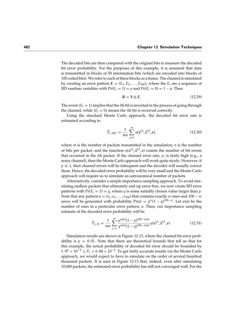
482 Chapter 12 Simulation Techniques
The decoded bits are then compared with the original bits to measure the decodedbit error probability. For the purposes of this example, it is assumed that datais transmitted in blocks of 50 information bits (which are encoded into blocks of100 coded bits). We refer to each of these blocks as a frame. The channel is simulatedby creating an error pattern E = (E1, E2, . . . , E100), where the Ei are a sequence ofIID random variables with Pr(Ei = 1) = p and Pr(Ei = 0) = 1 − p. Then
R = Y ⊕ E. (12.29)
The event {Ei = 1} implies that the ith bit is inverted in the process of going throughthe channel, while {Ei = 0} means the ith bit is received correctly.
Using the standard Monte Carlo approach, the decoded bit error rate isestimated according to
Pe, MC = 1mn
m∑j=1
η(x(j), x(j), e), (12.30)
where m is the number of packets transmitted in the simulation; n is the numberof bits per packet; and the function η(x(j), x(j), e) counts the number of bit errorsthat occurred in the jth packet. If the channel error rate, p, is fairly high (e.g., anoisy channel), then the Monte Carlo approach will work quite nicely. However, ifp � 1, then channel errors will be infrequent and the decoder will usually correctthem. Hence, the decoded error probability will be very small and the Monte Carloapproach will require us to simulate an astronomical number of packets.
Alternatively, consider a simple importance sampling approach. To avoid sim-ulating endless packets that ultimately end up error-free, we now create IID errorpatterns with Pr(Ei = 1) = q, where q is some suitably chosen value larger than p.Note that any pattern e = (e1, e2, . . . , e100) that contains exactly w ones and 100 − wzeros will be generated with probability Pr(e) = qw(1 − q)100−w. Let w(e) be thenumber of ones in a particular error pattern, e. Then, our importance samplingestimate of the decoded error probability will be
Pe, IS = 1mn
m∑j=1
pw(e)(1 − p)100−w(e)
qw(e)(1 − q)100−w(e)η(x(j), x(j), e). (12.31)
Simulation results are shown in Figure 12.13, where the channel bit error prob-ability is p = 0. 01. Note that there are theoretical bounds that tell us that forthis example, the actual probability of decoded bit error should be bounded by1. 97 × 10−5 ≤ Pe ≤ 6. 84 × 10−5. To get fairly accurate results via the Monte Carloapproach, we would expect to have to simulate on the order of several hundredthousand packets. It is seen in Figure 12.13 that, indeed, even after simulating10,000 packets, the estimated error probability has still not converged well. For the
Exercises 483
0 2,000 4,000 6,000 8,000 10,000
10–3
Packets
Est
imat
ed p
roba
bilit
y of
bit
erro
r
Importance sampling
S t andard Monte Carlo
10–4
10–5
10–6
Figure 12.13 Simulation results for a coded digital communications system using standardMonte Carlo and importance sampling techniques.
importance sampling results, we used q = 0. 05 so that important error eventsoccurred much more frequently. As seen in the figure, the estimated error prob-ability has converged rather nicely after simulating only a few thousand packets.Hence, for this example, using the importance sampling method has sped up thesimulation time by a few orders of magnitude.
Exercises12.1 Consider the periodic sequence generated by the four-stage shift register
in Figure 12.1. Suppose the sequence is converted to ±1-valued sequenceby mapping all 1s to −1s and all 0s to 1s. One period of the resultingsequence is
−1, −1, −1, −1, 1, 1, 1, −1, 1, 1, −1, −1, 1, −1, 1.

484 Chapter 12 Simulation Techniques
Calculate the autocorrelation function of this periodic sequence. Hint: Donot just treat this sequence as having finite length. The sequence is infinitein both directions. The finite sequence shown is just one period of theinfinite periodic sequence.
12.2 Sketch the shift register described by the octal number 75. Find thesequence output by this shift register assuming that the shift register isinitially loaded with all ones.
12.3 A certain N-stage shift register has its tap connections configured so thatit produces an m-sequence. The shift register is initially loaded with thecontents c = (c0, c1, . . . , cN−1), resulting in a periodic sequence of period2N − 1. Prove that if the shift register is loaded with some other contentsc′ �= 0, the new output sequence will be a cyclic shift of the original outputsequence. Hint: Recall that for an m-sequence, the shift register must cyclethrough all nonzero states.
12.4 Suppose we create a binary ±1 valued sequence of length N by drawing Nindependent realizations of a Bernoulli random variable to form one periodof the sequence. Compute the autocorrelation function of this randomBernoulli sequence.
12.5 Suppose a pseudorandom sequence is constructed using the power residuemethod as described by
xk = axk−1 mod q, k = 1, 2, 3, . . . .
Find the period and the sequence that results for the following values of(a, q). For each case, assume the seed is xo = 1.
(a) a = 4, q = 9,
(b) a = 5, q = 9,
(c) a = 2, q = 5,
(d) a = 5, q = 11.
12.6 Suppose a pseudorandom sequence is constructed using the power residuemethod as discussed in Exercise 12.5. If q = 11, find a value of a that leadsto a sequence with maximum possible period.
12.7 Find a transformation that will change a uniform random variableinto each of the following distributions (see Appendix D, Summary of

Exercises 485
Common Random Variables, for the definitions of these distributions ifnecessary):
(a) arcsine,
(b) Cauchy,
(c) Rayleigh,
(d) geometric.
12.8 Suppose we wish to generate a 10-msec realization of a zero-meanGaussian random process with a PSD of
S(f ) = 11 + (f /f3)2 .
(a) Find the bandwidth that contains 99 percent of the total power in therandom process.
(b) Determine how many frequency samples are needed for the frequencydomain method described in Section 12.2A.
12.9 Suppose we wanted to generate the random process whose PSD is givenin Exercise 12.8 using the time domain method discussed in Section 12.2B.
(a) Find the transfer function of the analog filter that will produce thedesired output PSD when the input is a zero-mean, white Gaussianrandom process.
(b) Use a bilinear transformation to convert the analog filter to a digitalfilter.
(c) What is the approximate duration of the impulse response of the digitalfilter if the 3-dB frequency of the random process is f3 = 1 kHz?
12.10 Suppose we use a Monte Carlo simulation approach to simulate the prob-ability of some rare event A. It is decided that we will repeat the simulationuntil the event A occurs 35 times. With what accuracy will we estimate pA
to within a 90 percent confidence level?
12.11 Prove that the importance sampling (IS) estimator of Equation 12.26 isunbiased. That is, show that
E[pA, IS] = pA.

486 Chapter 12 Simulation Techniques
MATLAB Exercises12.12 We wish to generate a periodic sequence of numbers that cycles through
the integers from 1 to 100 in a pseudorandom fashion. Choose a pair ofintegers (a, q) that can be used in the power residue method to produce asequence of the desired form. Write a MATLAB program to verify that thesequence produced does in fact cycle through each of the integers 1 to 100exactly once each before the sequence repeats.
12.13 Let X ∼ N(2, 1), Y ∼ N(0, 1), Z ∼ N(0, 1), and W =√
X2 + Y2 + Z2.We desire to find Pr(W > 3). Write a MATLAB program to estimate thisprobability through Monte Carlo simulation techniques. If we want to be90 percent sure that our estimate is within 5 percent of the true value,about how many times should we observe the event {W > 3}? Run yourprogram and provide the estimate of the desired probability. Can you findthe probability analytically?
12.14 Write a MATLAB program to generate a realization of the random processfrom Exercise 12.8 (using the frequency domain method). Use a peri-odogram to estimate the PSD of the process using the realization of theprocess you generated. Does your PSD estimate agree with the PSD thatthe process is designed to possess?
12.15 Write a MATLAB program to generate a realization of the random processfrom Exercise 12.9 (using the time domain method). Use a periodogramto estimate the PSD of the process using the realization of the process yougenerated. Does your PSD estimate agree with the PSD that the process isdesigned to possess?

Review of Set Theory A
The purpose for reviewing set theory is to provide a mathematical structure fororganizing methods of counting and grouping objects. Set theory may be usedto define the probabilities of possible outcomes of experiments. There are twocommon methods for defining a set. The first method, known as the roster method,is to list the elements of a set. Synonyms for sets include class, aggregate, andcollection. We will denote sets by capital letters, A, B, C, and so forth. The elementsof a set will be indicated by lowercase letters, such as a, b, c, and so forth. If a is anelement (or object, or member, or point) of A, then we denote this as a ∈ A. If a isnot an element of A, the notation is a ∈ A. A second way of defining a set is calledthe property method, which describes some property held by all elements of the setbut not held by objects that do not belong to the set.
DEFINITION A.1: A set A is said to be a subset of another set, B, if all elements ofA are also in B, in which case we write A ⊆ B. With this definition, it is possible thatthe two sets are equal (i.e., they have all the same elements), in which case A ⊆ Band at the same time B ⊆ A. If on the other hand, A is a subset of B and there aresome elements of B that are not in A, then we say that A is a proper subset of B andwe write A ⊂ B.
DEFINITION A.2: The universal set, S, is the set of all objects under considerationin a given problem, while the empty set, Ø, is the set that contains no elements.
DEFINITION A.3: The complement of a set A, written A, is the set of all elementsin S that are not in A. For two sets A and B that satisfy A ⊂ B, the difference set,written B − A, is the set of elements in B that are not in A.
Note that for any set A, Ø ⊆ A ⊆ S and A ⊆ A. Also, if A ⊆ B and B ⊆ C, thenA ⊆ C. Finally, we also note the relationship S = Ø.
487
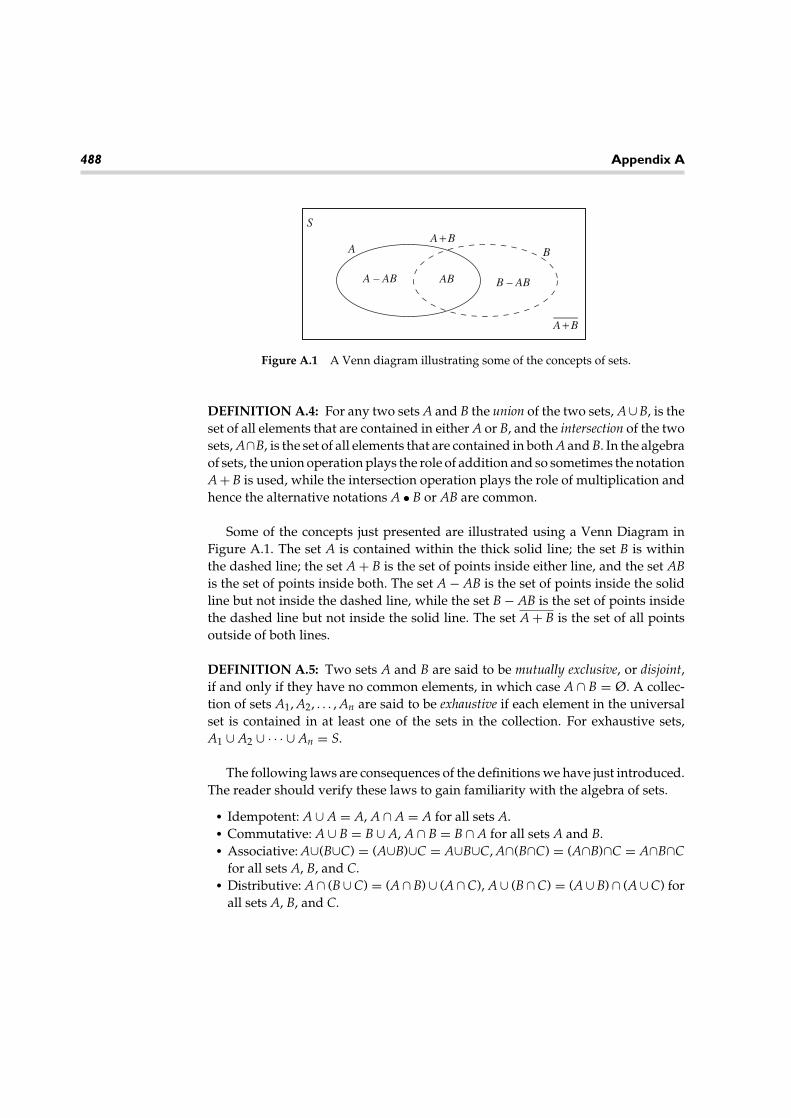
488 Appendix A
S
A B
ABA – AB
A + B
A + B
B – AB
Figure A.1 A Venn diagram illustrating some of the concepts of sets.
DEFINITION A.4: For any two sets A and B the union of the two sets, A ∪ B, is theset of all elements that are contained in either A or B, and the intersection of the twosets, A∩B, is the set of all elements that are contained in both A and B. In the algebraof sets, the union operation plays the role of addition and so sometimes the notationA + B is used, while the intersection operation plays the role of multiplication andhence the alternative notations A • B or AB are common.
Some of the concepts just presented are illustrated using a Venn Diagram inFigure A.1. The set A is contained within the thick solid line; the set B is withinthe dashed line; the set A + B is the set of points inside either line, and the set ABis the set of points inside both. The set A − AB is the set of points inside the solidline but not inside the dashed line, while the set B − AB is the set of points insidethe dashed line but not inside the solid line. The set A + B is the set of all pointsoutside of both lines.
DEFINITION A.5: Two sets A and B are said to be mutually exclusive, or disjoint,if and only if they have no common elements, in which case A ∩ B = Ø. A collec-tion of sets A1, A2, . . . , An are said to be exhaustive if each element in the universalset is contained in at least one of the sets in the collection. For exhaustive sets,A1 ∪ A2 ∪ · · · ∪ An = S.
The following laws are consequences of the definitions we have just introduced.The reader should verify these laws to gain familiarity with the algebra of sets.
• Idempotent: A ∪ A = A, A ∩ A = A for all sets A.• Commutative: A ∪ B = B ∪ A, A ∩ B = B ∩ A for all sets A and B.• Associative: A∪(B∪C) = (A∪B)∪C = A∪B∪C, A∩(B∩C) = (A∩B)∩C = A∩B∩C
for all sets A, B, and C.• Distributive: A ∩ (B ∪ C) = (A ∩ B) ∪ (A ∩ C), A ∪ (B ∩ C) = (A ∪ B) ∩ (A ∪ C) for
all sets A, B, and C.

Review of Set Theory 489
• Consistency: The three conditions A ⊆ B, A ∩ B = A, and A ∪ B = B are allconsistent or mutually equivalent.
• Universal bounds: Ø ⊆ A ⊆ S for all sets A.• Product: Ø ∩ A = Ø, S ∩ A = A for all sets A.• Sum: Ø ∪ A = A, S ∪ A = S for all sets A.• Involution: (A) = A for all sets A.• Complementarity: A ∪ A = S, A ∩ A = Ø for all sets A.• DeMorgan’s first law: A ∪ B = A ∩ B for all sets A and B.• DeMorgan’s second law: A ∩ B = A ∪ B for all sets A and B.
DeMorgan’s laws can be stated as follows: To find the complement of an expression,replace each set by its complement and interchange additions with multiplicationsand multiplications with additions.

Review of Linear Algebra B
The study of probability and random processes draws heavily upon concepts andresults from elementary linear algebra. In the main text, we assume that the readerhas a working knowledge of undergraduate-level linear algebra. The aim of thisappendix is to provide a review for those who need to brush up on these concepts.This review is not intended to be an exhaustive treatment of the topic, but ratheris a summary of selected concepts that are used within the text.
DEFINITION B.1: A matrix is a two dimensional array of numbers. We say thata matrix has size m × n if the array has m rows and n columns. If the matrix hasonly one row, then we refer to it as a row vector, while if there is only one columnit is a column vector. A matrix with one row and one column is called a scalar. Theelements of a matrix, B, are written as bi,j, where the first subscript represents therow number and the second subscript gives the column number.
DEFINITION B.2: The transpose of a matrix is obtained by exchanging the rowand column number of each element. That is, if matrix B has elements bi,j, then theelement in the ith row and jth column of BT is bj,i. Hence, if a matrix has size m × n,then its transpose has size n × m. Also, the transpose of a column vector is a rowvector and the transpose of a row vector is a column vector. A matrix B is said tobe symmetric if BT = B.
DEFINITION B.3: The Hermitian transpose (or just Hermitian) of a matrix B iswritten BH and is formed by taking the complex conjugate of the transpose. Thatis, if matrix B has elements bi,j, then the element in the ith row and jth column ofBH is b∗
j,i. A matrix B is said to be Hermitian symmetric if BH = B. Sometimes sucha matrix is simply called a Hermitian matrix.
491

492 Appendix B
DEFINITION B.4: Addition and multiplication of matrices is defined as follows.If two matrices A and B have the same size (i.e., the same number of rows andcolumns), then their sum is defined as C = A + B where ci,j = ai,j + bi,j. That is,matrix addition is done on an element by element basis. If the two matrices do nothave the same dimensions, they cannot be added. If A has size m × k and B hassize k × n, then their product, C = AB, will be an m × n matrix whose elements aregiven by
ci,j =k∑
l=1
ai,lbl,j. (B.1)
In order for the matrix product AB to be defined, the number of columns in A mustequal the number of rows in B.
It is also common to define two different products involving vectors, the so-called scalar (or dot) product and the matrix (or cross) product. We have no occasionto use the cross product in this text and so we do not consider it here. For twocolumn vectors a and b (both with the same number of elements), the dot productis defined as a • b = aHb, where the standard definition of matrix multiplicationas it applies to vectors is used. Two vectors are said to be orthogonal if their dot
product is zero. Finally, the norm of a vector is ||b|| =√
bHb.With these definitions in place, the reader should be able to verify the following
properties of matrix arithmetic.
• Commutative: A + B = B + A for matrices for which the addition is defined.However, the same property does not usually hold for multiplication. That is,AB does not necessarily equal BA. In fact, BA may not even be defined.
• Associative: A + (B + C) = (A + B) + C and A(BC) = (AB)C.• Distributive: A(B + C) = AB + AC.• Transposes of sums: (A + B)T = AT + BT and (A + B)H = AH + BH .• Transposes of products: (AB)T = BTAT and (AB)H = BHAH .
In much of this text, many of the matrices we deal with are square. The fol-lowing definition identifies some characteristics that can be applied to squarematrices.
DEFINITION B.5: A matrix B is diagonal if its elements satisfy bi,j = 0 for all i �= j.A matrix is upper triangular if bi,j = 0 for all i > j and lower triangular if bi,j = 0 forall i < j. Note that a diagonal matrix is simultaneously upper and lower triangular.Finally, a matrix is an m×m identity matrix if it is a diagonal matrix whose diagonalentries are all equal to 1. The letter I is reserved to represent an identity matrix.
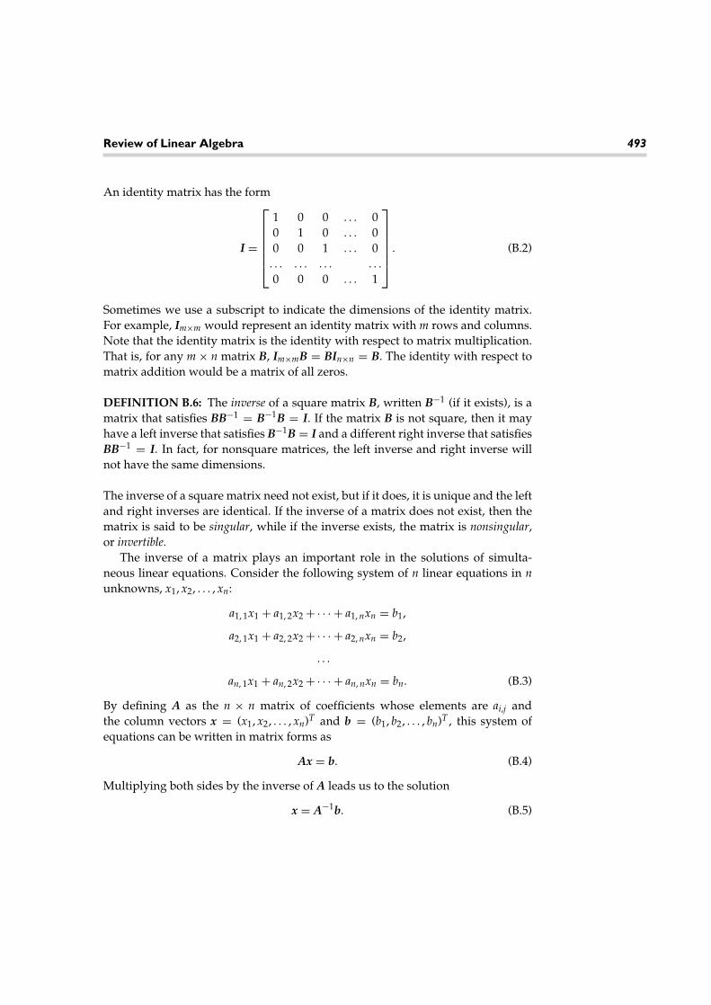
Review of Linear Algebra 493
An identity matrix has the form
I =
1 0 0 . . . 00 1 0 . . . 00 0 1 . . . 0
. . . . . . . . . . . .0 0 0 . . . 1
. (B.2)
Sometimes we use a subscript to indicate the dimensions of the identity matrix.For example, Im×m would represent an identity matrix with m rows and columns.Note that the identity matrix is the identity with respect to matrix multiplication.That is, for any m × n matrix B, Im×mB = BIn×n = B. The identity with respect tomatrix addition would be a matrix of all zeros.
DEFINITION B.6: The inverse of a square matrix B, written B−1 (if it exists), is amatrix that satisfies BB−1 = B−1B = I. If the matrix B is not square, then it mayhave a left inverse that satisfies B−1B = I and a different right inverse that satisfiesBB−1 = I. In fact, for nonsquare matrices, the left inverse and right inverse willnot have the same dimensions.
The inverse of a square matrix need not exist, but if it does, it is unique and the leftand right inverses are identical. If the inverse of a matrix does not exist, then thematrix is said to be singular, while if the inverse exists, the matrix is nonsingular,or invertible.
The inverse of a matrix plays an important role in the solutions of simulta-neous linear equations. Consider the following system of n linear equations in nunknowns, x1, x2, . . . , xn:
a1, 1x1 + a1, 2x2 + · · · + a1, nxn = b1,
a2, 1x1 + a2, 2x2 + · · · + a2, nxn = b2,
. . .
an, 1x1 + an, 2x2 + · · · + an, nxn = bn. (B.3)
By defining A as the n × n matrix of coefficients whose elements are ai,j andthe column vectors x = (x1, x2, . . . , xn)T and b = (b1, b2, . . . , bn)T , this system ofequations can be written in matrix forms as
Ax = b. (B.4)
Multiplying both sides by the inverse of A leads us to the solution
x = A−1b. (B.5)

494 Appendix B
Hence, if the coefficient matrix is invertible, the system has a unique solution. Onthe other hand, if the coefficient matrix is singular, then A−1 does not exist and theset of equations does not have a unique solution. This would be the case if someof the equations in Equation B.3 were linearly dependent (redundant), in whichcase the system would have more than one solution, or if some of the equationswere inconsistent, which would lead to no solution. In either case of redundant orinconsistent equations, the rows of the A matrix will be linearly dependent and theinverse will not exist. Conversely, if the rows of A are linearly independent, thematrix will be invertible.
A few properties of matrices that are related to the inverse are
• Inverse of transposes: (AT )−1 = (A−1)T .• Inverse of Hermitian transposes: (AH)−1 = (A−1)H .• Inverse of products: (AB)−1 = B−1A−1.• Inverse of identities: I−1 = I.
A single quantity that is extremely useful in characterizing the invertibility ofa matrix is its determinant. The determinant can be rather difficult to define in asimple manner, but it has many useful properties. We use a recursive definition,which may seem rather cryptic, but is probably the simplest definition and is alsoconsistent with how determinants are often calculated.
DEFINITION B.7: Let B be an n × n matrix with elements bi,j. Define B(i,j) to bethe (n − 1) × (n − 1) matrix obtained by removing the ith row and jth column fromB. Then the determinant of B is defined recursively according to
det(B) =n∑
j=1
(−1)i+jdet(B(i,j)), for any i = 1, 2, . . . , n. (B.6)
This recursion, together with the definition that for a 1×1 matrix B = [b], det(B) = b,is sufficient to calculate the determinant of any n × n matrix.
To see how this works, consider a 2 × 2 matrix:
det([
a bc d
])= adet([d]) − bdet([c]) = ad − bc. (B.7)
This result was obtained using i = 1 in Equation B.6. We could also have used i = 2and achieved the same result:
det([
a bc d
])= −cdet([b]) + ddet([a]) = −cb + da. (B.8)

Review of Linear Algebra 495
For a general 3 × 3 matrix, the determinant works out to be
det
a b cd e fg h i
= adet([
e fh i
])− bdet
([d fg i
])+ cdet
([d eg h
])
= a(ei − fh) − b(di − fg) + c(dh − eg). (B.9)
Probably the most important property of determinants is that if det(B) = 0, thenthe matrix B is singular, and conversely if det(B) �= 0, then B is invertible. This,along with some other important properties, is listed next. We will not prove anyof these properties in this review.
• Invertibility: {det(B) = 0} ⇐⇒ {B is singular}.• Row exchange: If the matrix A is formed by exchanging any two rows in the
matrix B, then det(A) = −det(B).• Identity matrices: For any identity matrix, det(I) = 1.• Triangular matrices: If B is a triangular matrix,
det(B) =n∏
i=1
bi,i.
That is, the determinant is the product of the diagonal elements. Note thatdiagonal matrices are a special case and this property applies to them as well.
• Products of matrices: det(AB) = det(A)det(B).• Inverses: det(B−1) = 1/det(B).• Transposes: det(BT ) = det(B).• Hermitian transposes: det(BH) = (det(B))∗.
In addition to computing determinants of matrices, we will also find needthroughout the text to compute eigenvalues and eigenvectors of square matrices.
DEFINITION B.8: For a square matrix B, the scalar λ is an eigenvalue and thevector x is a corresponding eigenvector if
Bx = λx. (B.10)
Note that the previous equation can be written in the slightly different form(B − λI)x = 0. The eigenvector x will be nonzero only if the matrix B − λI issingular. If it were nonsingular, we could multiply both sides by its inverse toobtain the trivial solution x = 0. Hence, the eigenvalues of the matrix B must besolutions to the equation
det(B − λI) = 0. (B.11)

496 Appendix B
This is the so-called characteristic equation for the matrix B. For an n × n matrix,B, the characteristic equation will be an nth order polynomial equation in λ, andhence an n × n matrix will have n eigenvalues (although some of them may berepeated). Corresponding to each eigenvalue, λk, is an eigenvector, xk. Note thatthe eigenvector is not unique since if xk satisfies Equation B.10, then any multipleof xk will also satisfy the same equation and hence will also be an eigenvector. Inorder to resolve this ambiguity, it is common to normalize the eigenvectors so that||x||2 = 1, but the vector is still an eigenvector even if it is not normalized. In thecase of repeated eigenvalues, there may also be corresponding eigenvectors thatdiffer by more than just a scale constant.
Before listing the important properties of eigenvalues and eigenvectors, it isnecessary to include one more definition.
DEFINITION B.9: A matrix B is positive definite if zHBz > 0 for any vector zand it is negative definite if zHBz < 0 for all z. If zHBz ≥ 0 then the matrix is referredto as positive semi-definite, and if zHBz ≤ 0 the matrix is negative semi-definite.
With this definition in place, we now list the following properties of eigenvaluesand eigenvectors.
• Trace of a matrix: trace(B) = ∑nk=1 bk, k = ∑n
k=1 λk. That is, the sum of theeigenvalues is equal to the sum of the diagonal elements of a matrix, also knownas its trace.
• Determinant of a matrix:
det(B) =n∏
k=1
λk
That is, the product of the eigenvalues is the determinant of a matrix. As aresult, any singular matrix must have at least one eigenvalue that is zero.
• Triangular matrices: If a matrix B is triangular (or diagonal), the eigenvaluesare just the diagonal entries, λk = bk,k.
• Positive and negative definite matrices: If B is positive definite, then its eigen-values are all real and positive; whereas, if B is positive semi-definite, all itseigenvalues are nonnegative. Similarly, if B is negative definite, then the eigen-values are negative; whereas, if B is negative semi-definite, the eigenvalues arenonpositive.
• Linear independence: If the eigenvectors x1, x2, . . . , xn are nonzero and corre-spond to distinct (not repeated) eigenvalues λ1, λ2, . . . , λn, then the eigenvectorsare linearly independent.
• Diagonal form: Suppose B is an n × n matrix and has n linearly independenteigenvectors. Construct a matrix S whose columns are the n eigenvectors and a

Review of Linear Algebra 497
diagonal matrix � whose diagonal entries are the eigenvalues. Then the matrixB can be factored as B = S�S−1.
• Powers of a matrix: A direct result of the previous property is that for matriceswith linearly independent eigenvectors, Bk = S�kS−1. Furthermore, since � isdiagonal, �k is computed by raising each diagonal entry to the kth power.
In many of the applications encountered in this text, the matrices we are dealingwith are Hermitian. These matrices posess additional properties that are not neces-sarily shared by all matrices, making Hermitian matrices particularly convenientto work with.
• Positive semi-definite: Any Hermitian matrix has all real eigenvalues and is atleast positive semi-definite. Furthermore, if the matrix is also nonsingular, thenit will be positive definite.
• Orthogonal eigenvectors: Eigenvectors of a Hermitian matrix that correspondto different eigenvalues are orthogonal.
• Spectral decomposition: Any Hermitian matrix can be decomposed into theform
B = U�UH =n∑
k=1
λkxkxHk , (B.12)
where U is the matrix whose columns are the eigenvectors (normalized).

Review of Signalsand Systems C
This appendix provides a summary of some important results in the area ofsignal representation and linear time–invariant systems. Any engineering studentembarking on a serious study of probability and random processes should be famil-iar with these concepts and hence a rigorous development is not attempted here.Rather this review is intended as a brief refresher for those who need it and alsoas a quick reference for some important results that are used throughout the text.In this appendix, attention is focused on deterministic signals and systems in bothcontinuous and discrete time.
DEFINITION C.1: Consider a periodic signal x(t) whose period is To. That isx(t) = x(t + To) for all t. The inverse of the period fo = 1/To is called the fundamentalfrequency of x(t) and any frequency, fn = nfo, that is a multiple of the fundamentalfrequency is called a harmonic.
Any periodic signal (subject to some mild constraints known as the Dirichletconditions) can be represented as a linear combination of complex exponential sig-nals, exp(j2π fnt), whose frequencies are at the harmonics of the signal. That is, ifx(t) is periodic with period To, then
x(t) =∞∑
k=−∞xne j2πnfot. (C.1)
This is known as the Fourier series expansion and the series coefficients can becomputed according to
xn = 1To
∫
To
x(t)e−j2πnfot dt. (C.2)
499

500 Appendix C
Since the signal is periodic, the integral in the previous expression can be taken overany convenient interval of length To. In general, the series coefficients are complexnumbers and it is common to express them in terms of their magnitude and phase,xn = ∣∣xn
∣∣ exp(j∠xn). The Fourier series coefficients display the frequency contentof periodic signals.
For signals that are not periodic, the Fourier transform can be used to displaythe frequency content of a signal. The Fourier transform of a signal is given by
X(f ) =∫ ∞
−∞x(t)e−j2π ft dt, (C.3)
and the inverse Fourier transform is
x(t) =∫ ∞
−∞X(f )ej2π ft df . (C.4)
Sometimes we use the notation x(t) ↔ X(f ) to indicate that x(t) and X(f ) are aFourier transform pair. A table of some common Fourier transform pairs is pro-vided in Appendix E, Mathematical Tables, Table E.1. Some of the more importantproperties of Fourier transforms are listed next.
• Linearity: If x(t) ↔ X(f ) and y(t) ↔ Y(f ), then ax(t) + by(t) ↔ aX(f ) + bY(f ) forany constants a and b.
• Symmetry: If x(t) is real-valued, then X(−f ) = X∗(f ). As a result, |X(f )| mustthen be an even function of f and ∠X(f ) must be an odd function of f . In addition,if x(t) is both real and even, then X(f ) will be real and even.
• Time shifting: If x(t) ↔ X(f ), then x(t − to) ↔ e−j2π fto X(f ). As a consequence,shifting a signal in time does not alter the magnitude of its Fourier transform.
• Differentiation: If x(t) ↔ X(f ), thendx(t)
dt↔ j2π fX(f ).
• Integration: If x(t) ↔ X(f ), then∫ t−∞ x(u)du ↔ X(f )
j2π f+ 1
2X(0)δ(f ). The term X(0)
that appears in this expression is the direct current (DC) value of the signal.
• Time and frequency scaling: If x(t) ↔ X(f ), then x(at) = 1|a|X
(fa
)for any
constant a �= 0.• Parseval’s relation: If x(t) ↔ X(f ), then
∫ ∞−∞ |x(t)|2 dt = ∫ ∞
−∞ |X(f )|2 df . This is astatement of conservation of energy. That is, the energy in the time domain isequal to the energy in the frequency domain.
• Convolution: If x(t) ↔ X(f ) and y(t) ↔ Y(f ), then
x(t) ∗ y(t) =∫ ∞
−∞x(u)y(t − u) dt ↔ X(f )Y(f ).

Review of Signals and Systems 501
For signals in discrete time, x[n], a discrete-time Fourier transform (DFT) is definedaccording to
X(f ) =∞∑
n=−∞x[n]e−j2π fn, (C.5)
and the inverse DFT is
x[n] =∫ 1/2
−1/2X(f )ej2π fn df . (C.6)
Since X(f ) is periodic with a period of 1, the integral in Equation C.5 can be takenover any interval of length 1. It is common to view the DFT using discrete frequencysamples as well. In that case, the definition of the DFT and its inverse is modifiedto give the N-point DFT:
X[m] =N−1∑
n=0
x[n]e−j2πmn/N , (C.7)
x[n] = 1N
N−1∑
m=0
X[m]ej2πmn/N . (C.8)
Alternatively, by replacing exp(j2π f ) with z in the definition of the DFT, we getthe z-transform:
X(z) =∞∑
n=−∞x[n]z−n. (C.9)
The inverse z-transform is given by a complex contour integral,
x[n] = 12π j
∮X(z)zn−1 dz, (C.10)
where the contour of integration is any closed contour that encircles the origin inthe counterclockwise direction and is within the region of convergence of X(z).Because of the complicated nature of the inverse transform, it is common to com-pute these inverse transforms via tables. A table of some common z-transform pairsis provided in Appendix E, Mathematical Tables, Table E.2.
These various transform representations of signals are particularly useful whenstudying the passage of signals through linear time–invariant (LTI) systems.
DEFINITION C.2: Suppose when x(t) is input to a system, the output is y(t). Thesystem is said to be time-invariant if the input x(t−to) produces an output of y(t−to).

502 Appendix C
That is, a time delay in the input produces the same time delay on the output but noother changes to the output. Furthermore, suppose the two inputs x1(t) and x2(t)produce the two outputs y1(t) and y2(t), respectively. Then, the system is linear ifthe input ax1(t) + bx2(t) produces the output ay1(t) + by2(t) for any constants a andb. Identical definitions apply to discrete time systems as well.
A direct consequence of the linearity of a system is the concept of superposition,which states that if the input can be written as a linear combination of severalterms x(t) = a1x1(t) + a2x2(t) + · · · + anxn(t), then the corresponding output canbe written as the same linear combination of the corresponding outputs y(t) =a1y1(t) + a2y2(t) + · · · + anyn(t).
Any LTI system can be described in terms of its impulse response, h(t). If theinput is a delta (impulse) function, δ(t), the output is then the impulse responsey(t) = h(t). For any LTI system, the input/output relationship is given in terms ofthe impulse response according to the convolution integral
y(t) = x(t) ∗ h(t) =∫ ∞
−∞x(u)h(t − u) du =
∫ ∞
−∞x(t − u)h(u) du. (C.11)
If the input is a complex exponential at some frequency f (i.e., x(t) = exp(j2π ft)),then the corresponding output is then
y(t) = e j2π ft∫ ∞
−∞h(u)e−j2π fudu = ej2π ftH(f ). (C.12)
That is, the output will also be a complex exponential whose magnitude and phasehave been adjusted according to the complex number H(f ). This function of fre-quency is called the transfer function of the system and is the Fourier transform ofthe impulse response. Since complex exponentials form eigenfunctions of any LTIsystem, when studying LTI systems, it is convenient to decompose signals intolinear combinations of complex exponentials. If x(t) is a periodic signal it can bewritten as a linear combination of complex exponentials through its Fourier seriesrepresentation,
x(t) =∑
k
xke j2πkfot. (C.13)
Using the concept of superposition together with the previous result, we find thatthe output of an LTI system when x(t) is input is
y(t) =∑
k
xkH(kfo)e j2πkfot =∑
k
yke j2πkfot. (C.14)
Hence, the Fourier series coefficients of the input and output of an LTI system arerelated by the simple form
yk = xkH(kfo). (C.15)

Review of Signals and Systems 503
A similar relationship holds for the Fourier transforms of nonperiodic signals.Taking Fourier transforms of both sides of Equation C.11 and using the convolutionproperty of Fourier transforms results in
Y(f ) = X(f )H(f ). (C.16)
Identical relationships hold for the DFT and z-transforms as well.

Summary of CommonRandom Variables D
This appendix provides a quick reference of some of the most common randomvariables. Special functions that are used in this appendix are defined in thefollowing list.
• Gamma function: �(α) = ∫ ∞0 uα−1e−u du, Re[α] > 0.
• Incomplete gamma function: γ (α, β) = ∫ β
0 uα−1e−u du, Re[α] > 0.
• Beta function: B(a, b) = ∫ 10 ua−1(1 − u)b−1du = �(a)�(b)
�(a + b).
• Incomplete beta function: β(a, b, x) = ∫ x0 ua−1(1 − u)b−1du, 0 < x < 1.
• Modified Bessel function of order m: Im(x) = 12π
∫ 2π
0 ex cos(θ ) cos(mθ ) dθ .
• Q-function: Q(x) = ∫ ∞x
12π
exp(−u2
2
)du.
• Marcum’s Q-function: Q(α, β) = ∫ ∞β
u exp
(
−α2 + u2
2
)
I0(αu) du.
D.1 Continuous Random Variables
D.1.1 Arcsine
For any b > 0,
fX(x) = 1
π√
b2 − x2− b < x < b. (D.1)
505

506 Appendix D
FX(x) =
0 x < −b12
+ 1π
sin−1(x
b
)−b ≤ x ≤ b
1 x > b
. (D.2)
µX = 0, σ 2X = b2
2. (D.3)
Note:
(1) Formed by a transformation X = b cos(2πU + θ ), where b and θ are constantsand U is a uniform random variable over [0, 1).
D.1.2 Beta
For any a > 0 and b > 0,
fX(x) = 1B(a, b)
xa−1(1 − x)b−1, 0 < x < 1. (D.4)
FX(x) =
0 x < 0β(a, b, x)B(a, b)
0 ≤ x ≤ 1
1 x > 1
. (D.5)
µX = aa + b
, σ 2X = ab
(a + b)2(a + b + 1). (D.6)
D.1.3 Cauchy
For any b > 0,
fX(x) = b/π
b2 + x2 . (D.7)
FX(x) = 12
+ 1π
tan−1(x
b
). (D.8)
�X(ω) = e−b|ω|. (D.9)
Notes:
(1) Both the mean and variance are undefined.(2) Formed by a transformation of the form X = b tan(2πU), where U is uniform
over [0, 1).

Summary of Common Random Variables 507
D.1.4 Chi-Square
For integer n > 0,
fX(x) = xn/2−1
2n/2�(n/2)e−x/2, x ≥ 0. (D.10)
FX(x) =
0 x < 0γ (n/2, x/2)
�(n/2)x ≥ 0
. (D.11)
�X(ω) = 1(1 − 2jω)n/2
. (D.12)
µX = n, σ 2X = 2n. (D.13)
Notes:
(1) The chi-square random variable is a special case of the gamma randomvariable.
(2) The parameter n is referred to as the number of degrees of freedom of thechi-square random variable.
(3) The chi-square random variable is formed by a transformation of the formX = ∑n
k=1 Z2k , where the Zk are independent and identically distributed (IID),
zero-mean, unit variance Gaussian random variables.
D.1.5 Erlang
For any integer n > 0 and any b > 0,
fX(x) = bnxn−1e−bx
(n − 1)! , x ≥ 0. (D.14)
FX(x) =
0 x < 0γ (n, bx)(n − 1)! x ≥ 0
. (D.15)
�X(ω) = 1(1 − jω/b)n . (D.16)
µX = n/b, σ 2X = n/b2. (D.17)
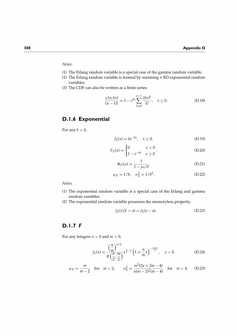
508 Appendix D
Notes:
(1) The Erlang random variable is a special case of the gamma random variable.(2) The Erlang random variable is formed by summing n IID exponential random
variables.(3) The CDF can also be written as a finite series
γ (n, bx)(n − 1)! = 1 − ebx
n−1∑
k=0
(bx)k
k! , x ≥ 0. (D.18)
D.1.6 Exponential
For any b > 0,
fX(x) = be−bx, x ≥ 0. (D.19)
FX(x) ={
0 x < 0
1 − e−bx x ≥ 0. (D.20)
�X(ω) = 11 − jω/b
. (D.21)
µX = 1/b, σ 2X = 1/b2. (D.22)
Notes:
(1) The exponential random variable is a special case of the Erlang and gammarandom variables.
(2) The exponential random variable possesses the memoryless property,
fX(x|X > a) = fX(x − a). (D.23)
D.1.7 F
For any integers n > 0 and m > 0,
fX(x) =( n
m
)n/2
B(n
2,
m2
)xn2 −1
(1 + n
mx)− n+m
2 , x > 0. (D.24)
µX = mm − 2
for m > 2, σ 2X = m2(2n + 2m − 4)
n(m − 2)2(m − 4)for m > 4. (D.25)

Summary of Common Random Variables 509
Notes:
(1) If U and V are independent chi-square random variables with n and m degreesof freedom, respectively, then F = (U/n)/(V/m) will be an F random variablewith n and m degrees of freedom.
D.1.8 Gamma
For any a > 0 and b > 0,
fX(x) = baxa−1e−bx
�(a), x ≥ 0. (D.26)
FX(x) = γ (a, bx)�(a)
. (D.27)
�X(ω) = 1(1 − jω/b)a . (D.28)
µX = a/b, σ 2X = a/b2. (D.29)
Note:
(1) The gamma random variable contains the chi-square, Erlang, and exponentialrandom variables as special cases.
D.1.9 Gaussian
For any µ and any σ > 0,
fX(x) = 1√2πσ 2
exp
(
− (x − µ)2
2σ 2
)
. (D.30)
FX(x) = 1 − Q(
x − µ
σ
)
. (D.31)
�X(ω) = exp(
jωµ − 12ω2σ 2
)
. (D.32)
µX = µ, σ 2X = σ 2. (D.33)

510 Appendix D
D.1.10 Gaussian-Multivariate
For any n element column vector µ and any valid n × n covariance matrix C,
fX(x) = 1(2π )n/2det(C)
exp(
−12
(X − µ)TC−1(X − µ))
. (D.34)
�X(ω) = exp(
jµTω − 12ωTCω
)
. (D.35)
E[X] = µ, E[(X − µ)(X − µ)T ] = C. (D.36)
D.1.11 Laplace
For any b > 0,
fX(x) = b2
exp(−b|x|). (D.37)
FX(x) =
12
ebx x < 0
1 − 12
e−bx x ≥ 0. (D.38)
�X(ω) = 11 + (ω/b)2 . (D.39)
µX = 0, σ 2X = 2/b2. (D.40)
D.1.12 Log-Normal
For any µ and any σ > 0,
fX(x) = 1
x√
2πσ 2exp
(
− (ln(x) − µ)2
2σ 2
)
, x > 0. (D.41)
FX(x) =
0 x < 0
1 − Q(
ln(x) − µ
σ
)
x ≥ 0. (D.42)
µX = exp
(
µ + σ 2
2
)
, σ 2X = [exp(σ 2) − 1] exp(2µ + σ 2). (D.43)

Summary of Common Random Variables 511
Notes:
(1) The log-normal random variable is formed by a transformation of the formX = exp(Z), where Z is a Gaussian random variable with mean µ andvariance σ 2.
(2) It is common to find instances in the literature where σ is referred to as thestandard deviation of the log-normal random variable. This is a misnomer. Thequantity σ is not the standard deviation of the log-normal random variable, butrather is the standard deviation of the underlying Gaussian random variable.
D.1.13 Nakagami
For any b > 0 and m > 0,
fX(x) = 2mm
�(m)bm x2m−1 exp(−m
bx2
), x ≥ 0. (D.44)
FX(x) =
0 x < 0
γ(
m,mb
x2)
�(m)x ≥ 0
. (D.45)
µX = �(m + 1/2)�(m)
√bm
, σ 2X = b − µ2
X . (D.46)
D.1.14 Rayleigh
For any σ > 0,
fX(x) = xσ 2 exp
(
− x2
2σ 2
)
, x ≥ 0. (D.47)
FX(x) =
0 x < 0
1 − exp
(
− x2
2σ 2
)
x ≥ 0. (D.48)
µX =√
πσ 2
2, σ 2
X = (4 − π )σ 2
2. (D.49)
Notes:
(1) The Rayleigh random variable arises when performing a Cartesian to polartransformation of two independent, zero-mean Gaussian random variables.
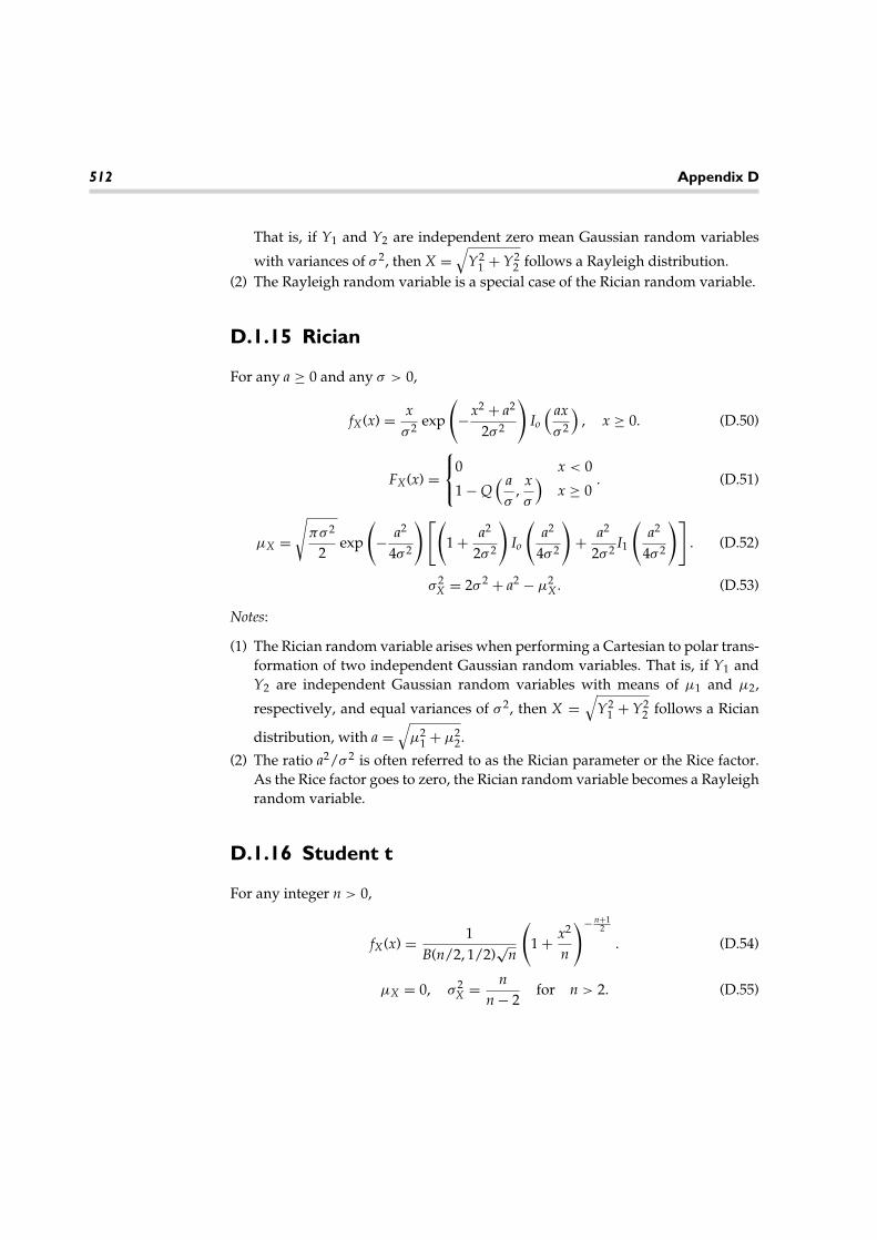
512 Appendix D
That is, if Y1 and Y2 are independent zero mean Gaussian random variables
with variances of σ 2, then X =√
Y21 + Y2
2 follows a Rayleigh distribution.(2) The Rayleigh random variable is a special case of the Rician random variable.
D.1.15 Rician
For any a ≥ 0 and any σ > 0,
fX(x) = xσ 2 exp
(
−x2 + a2
2σ 2
)
Io
( axσ 2
), x ≥ 0. (D.50)
FX(x) =
0 x < 0
1 − Q( aσ
,xσ
)x ≥ 0
. (D.51)
µX =√
πσ 2
2exp
(
− a2
4σ 2
) [(
1 + a2
2σ 2
)
Io
(a2
4σ 2
)
+ a2
2σ 2 I1
(a2
4σ 2
)]
. (D.52)
σ 2X = 2σ 2 + a2 − µ2
X . (D.53)
Notes:
(1) The Rician random variable arises when performing a Cartesian to polar trans-formation of two independent Gaussian random variables. That is, if Y1 andY2 are independent Gaussian random variables with means of µ1 and µ2,
respectively, and equal variances of σ 2, then X =√
Y21 + Y2
2 follows a Rician
distribution, with a =√
µ21 + µ2
2.
(2) The ratio a2/σ 2 is often referred to as the Rician parameter or the Rice factor.As the Rice factor goes to zero, the Rician random variable becomes a Rayleighrandom variable.
D.1.16 Student t
For any integer n > 0,
fX(x) = 1B(n/2, 1/2)
√n
(
1 + x2
n
)− n+12
. (D.54)
µX = 0, σ 2X = n
n − 2for n > 2. (D.55)

Summary of Common Random Variables 513
Notes:
(1) This distribution was first published by W. S. Gosset in 1908 under thepseudonym “A. Student.’‘ Hence, this distribution has come to be known asthe student’s t-distribution.
(2) The parameter n is referred to as the number of degrees of freedom.(3) If Xi i = 1, 2, . . . , n is a sequence of IID Gaussian random variables and µ
and s2 are the sample mean and sample variance, respectively, then the ratio
T = (µ − µ)/√
s2/n will have a t-distribution with n − 1 degrees of freedom.
D.1.17 Uniform
For any a < b,
fX(x) = 1b − a
, a ≤ x < b. (D.56)
FX(x) =
0 x < ax − ab − a
a ≤ x ≤ b
1 x > b
. (D.57)
�X(ω) = e jbω − e jaω
jω(b − a). (D.58)
µx = a + b2
, σ 2X = (b − a)2
12. (D.59)
D.1.18 Weibull
For any a > 0 and any b > 0,
fX(x) = abxb−1 exp(−axb), x ≥ 0. (D.60)
FX(x) ={
0 x < 0
1 − exp(−axb) x ≥ 0. (D.61)
µX =�
(
1 + 1b
)
a1/b, σ 2
X =�
(
1 + 2b
)
−[
�
(
1 + 1b
)]2
a2/b. (D.62)

514 Appendix D
Note:
(1) The Weibull random variable is a generalization of the Rayleigh randomvariable and reduces to a Rayleigh random variable when b = 2.
D.2 Discrete Random Variables
D.2.1 Bernoulli
For 0 < p < 1,
PX(k) =
1 − p k = 0
p k = 1
0 otherwise
. (D.63)
HX(z) = 1 − p(1 − z) for all z. (D.64)
µX = p, σ 2X = p(1 − p). (D.65)
D.2.2 Binomial
For 0 < p < 1 and any integer n > 0,
PX(k) =
(n
k
)
pk(1 − p)n−k k = 0, 1, 2, . . . , n
0 otherwise
. (D.66)
HX(z) = (1 − p(1 − z))n for any z. (D.67)
µx = np, σ 2X = np(1 − p). (D.68)
Note:
(1) The binomial random variable is formed as the sum of n independent Bernoullirandom variables.

Summary of Common Random Variables 515
D.2.3 Geometric
For 0 < p < 1,
PX(k) ={
(1 − p)pk k ≥ 0
0 k < 0. (D.69)
HX(z) = 1 − p1 − pz
for |z| < 1/p. (D.70)
µX = p1 − p
, σ 2X = p
(1 − p)2 . (D.71)
D.2.4 Pascal (or Negative Binomial)
For 0 < q < 1 and any integer n > 0,
PX(k) =
0 k < n(
k − 1
n − 1
)
(1 − q)nqk−n k = n, n + 1, n + 2, . . .. (D.72)
HX(z) =(
(1 − q)z1 − qz
)n
, for |z| < 1/q. (D.73)
µX = n1 − q
, σ 2X = nq
(1 − q)2 . (D.74)
D.2.5 Poisson
For any b > 0,
PX(k) =
bk
k! e−b k ≥ 0
0 k < 0. (D.75)
HX(z) = exp(b(z − 1)), for all z. (D.76)
µX = b, σ 2X = b. (D.77)
Mathematical Tables E
E.1 Trigonometric Identities
sin2(x) + cos2(x) = 1. (E.1)
cos(x ± y) = cos(x) cos(y) ∓ sin(x) sin(y). (E.2)
sin(x ± y) = sin(x) cos(y) ± cos(x) sin(y). (E.3)
cos(x) cos(y) = 12
cos(x + y) + 12
cos(x − y). (E.4)
sin(x) sin(y) = 12
cos(x − y) − 12
cos(x + y). (E.5)
sin(x) cos(y) = 12
sin(x + y) + 12
sin(x − y). (E.6)
exp(jx) = cos(x) + j sin(x). (E.7)
cos(x) = e jx + e−jx
2. (E.8)
sin(x) = e jx − e−jx
2j. (E.9)
E.2 Series Expansions
11 − x
=∞∑
k=0
xk, for |x| < 1. (E.10)
517
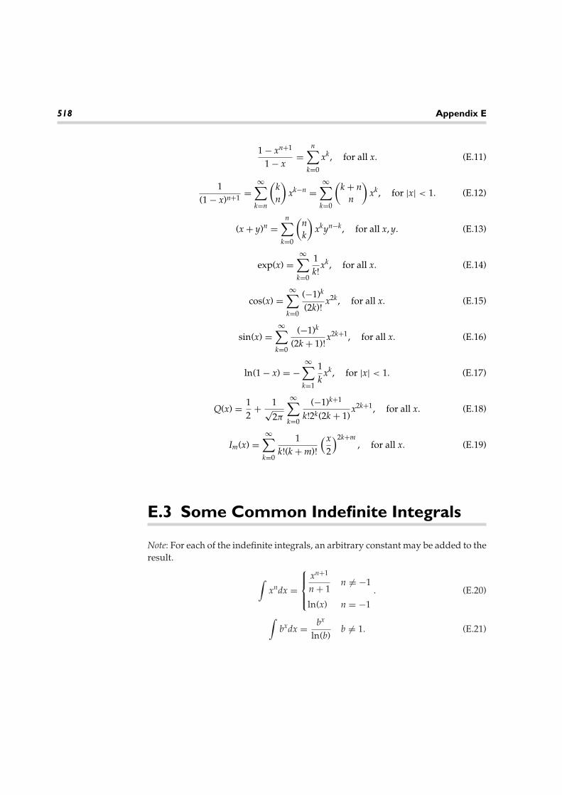
518 Appendix E
1 − xn+1
1 − x=
n∑
k=0
xk, for all x. (E.11)
1(1 − x)n+1 =
∞∑
k=n
(kn
)xk−n =
∞∑
k=0
(k + n
n
)xk, for |x| < 1. (E.12)
(x + y)n =n∑
k=0
(nk
)xkyn−k, for all x, y. (E.13)
exp(x) =∞∑
k=0
1k!xk, for all x. (E.14)
cos(x) =∞∑
k=0
(−1)k
(2k)! x2k, for all x. (E.15)
sin(x) =∞∑
k=0
(−1)k
(2k + 1)!x2k+1, for all x. (E.16)
ln(1 − x) = −∞∑
k=1
1k
xk, for |x| < 1. (E.17)
Q(x) = 12
+ 1√2π
∞∑
k=0
(−1)k+1
k!2k(2k + 1)x2k+1, for all x. (E.18)
Im(x) =∞∑
k=0
1k!(k + m)!
(x2
)2k+m, for all x. (E.19)
E.3 Some Common Indefinite Integrals
Note: For each of the indefinite integrals, an arbitrary constant may be added to theresult.
∫xndx =
xn+1
n + 1n �= −1
ln(x) n = −1. (E.20)
∫bxdx = bx
ln(b)b �= 1. (E.21)

Mathematical Tables 519
∫ln(x)dx = x ln(x) − x. (E.22)
∫sin(x)dx = − cos(x). (E.23)
∫cos(x)dx = sin(x). (E.24)
∫tan(x)dx = − ln(| cos(x)|). (E.25)
∫sinh(x)dx = cosh(x). (E.26)
∫cosh(x)dx = sinh(x). (E.27)
∫tanh(x)dx = ln(| cosh(x)|). (E.28)
∫eax sin(bx)dx = eax
(a sin(bx) − b cos(bx)
a2 + b2
). (E.29)
∫eax cos(bx)dx = eax
(b sin(bx) + a cos(bx)
a2 + b2
). (E.30)
∫xnebxdx = ebx
n∑
k=0
(−1)k
bk+1
n!(n − k)!xn−k (n ≥ 0). (E.31)
∫xn ln(bx)dx = xn+1
(ln(bx)n + 1
− 1(n + 1)2
)(n �= −1). (E.32)
∫1
x2 + b2 dx = 1b
tan−1(x
b
)(b > 0). (E.33)
∫1
√b2 − x2
dx = sin−1(x
b
)(b > 0). (E.34)
∫1
√x2 + b2
dx = log(x +√
x2 + b2) = sinh−1(x
b
)(b > 0). (E.35)
∫1
√x2 − b2
dx = log∣∣∣x +
√x2 − b2
∣∣∣ = cosh−1(x
b
)(b > 0). (E.36)
∫1
ax2 + bx + cdx =
1√
b2 − 4acln
∣∣∣∣∣2ax + b −
√b2 − 4ac
2ax + b +√
b2 − 4ac
∣∣∣∣∣ b2 > 4ac
2√
4ac − b2tan−1
(2ax + b
√4ac − b2
)b2 < 4ac
. (E.37)
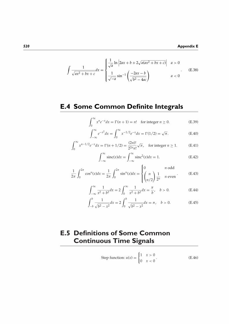
520 Appendix E
∫1
√ax2 + bx + c
dx =
1√a
ln∣∣∣2ax + b + 2
√a(ax2 + bx + c)
∣∣∣ a > 0
1√−asin−1
(−2ax − b√
b2 − 4ac
)a < 0
. (E.38)
E.4 Some Common Definite Integrals∫ ∞
0xne−xdx = �(n + 1) = n! for integer n ≥ 0. (E.39)
∫ ∞
−∞e−x2
dx =∫ ∞
0x−1/2e−xdx = �(1/2) = √
π . (E.40)
∫ ∞
0xn−1/2e−xdx = �(n + 1/2) = (2n)!
22nn!√
π , for integer n ≥ 1. (E.41)
∫ ∞
−∞sinc(x)dx =
∫ ∞
−∞sinc2(x)dx = 1. (E.42)
12π
∫ 2π
0cosn(x)dx = 1
2π
∫ 2π
0sinn(x)dx =
0 n odd(n
n/2
)12n n even
. (E.43)
∫ ∞
−∞1
x2 + b2 dx = 2∫ ∞
0
1x2 + b2 dx = π
b, b > 0. (E.44)
∫ b
−b
1√
b2 − x2dx = 2
∫ b
0
1√
b2 − x2dx = π , b > 0. (E.45)
E.5 Definitions of Some CommonContinuous Time Signals
Step function: u(x) ={
1 x > 0
0 x < 0. (E.46)

Mathematical Tables 521
Rectangle function: rect(x) ={
1 |x| < 1/2
0 |x| > 1/2. (E.47)
Triangle function: tri(x) ={
1 − |x| |x| ≤ 1
0 |x| > 1. (E.48)
Sinc function: sinc(x) = sin(πx)πx
. (E.49)
E.6 Fourier Transforms
Table E.1 Common Fourier Transform Pairs
Signal (time domain) Transform (frequency domain)
rect(t/to) tosinc(fto)
tri(t/to) tosinc2(fto)
exp(
− tto
)u(t)
to
1 + j2π fto
exp(
−|t|to
)2to
1 + (2π fto)2
sinc(t/to) torect(fto)
sinc2(t/to) totri(fto)
exp(j2π fot) δ(f − fo)
cos(2π fot + θ )12δ(f − fo)ejθ + 1
2δ(f + fo)e−jθ
δ(t − to) exp(−j2π fto)
sgn(t)1
jπ f
u(t)12δ(f ) + 1
j2π f
exp(−(t/to)2)√
π t2o exp(−(π fto)2)

522 Appendix E
E.7 z-Transforms
Table E.2 Common z-Transform Pairs
Signal Transform Region of convergence
δ[n] 1 all z
u[n] 11 − z−1 |z| > 1
nu[n] z−1
(1 − z−1
)2 |z| > 1
n2u[n] z−1(1 + z−1)(1 − z−1
)3 |z| > 1
n3u[n] z−1(1 + 4z−1 + z−2)(1 − z−1
)4 |z| > 1
bnu[n] 11 − bz−1 |z| > |b|
nbnu[n] bz−1
(1 − bz−1
)2 |z| > |b|
n2bnu[n] bz−1(1 + bz−1)(1 − bz−1
)3 |z| > |b|
bn cos[�on]u[n] 1 − b cos(�o)z−1
1 − 2b cos(�o)z−1 + bz−2 |z| > |b|
bn sin[�on]u[n] b sin(�o)z−1
1 − 2b cos(�o)z−1 + bz−2 |z| > |b|
u[n − 1]n
ln(
11 − z−1
)|z| > 1
(n + m
m
)bnu[n] 1
(1 − bz−1
)m+1 |z| > |b|
bn
n! u[n] exp(bz−1) all z

Mathematical Tables 523
E.8 Laplace Transforms
Table E.3 Common Laplace Transform Pairs
Function Transform Region of convergence
u(t) 1/s Re[s] > 0
exp(−bt)u(t)1
s + bRe[s] > −b
sin(bt)u(t)b
s2 + b2 Re[s] > 0
cos(bt)u(t)s
s2 + b2 Re[s] > 0
e−at sin(bt)u(t)b
(s + a)2 + b2 Re[s] > −a
e−at cos(bt)u(t)s + a
(s + a)2 + b2 Re[s] > −a
δ(t) 1 all s
ddt
δ(t) s all s
tnu(t), n ≥ 0n!
sn+1 Re[s] > 0
tne−btu(t), n ≥ 0n!
(s + b)n+1 Re[s] > −b

524 Appendix E
E.9 Q-Function
Table E.4 lists values of the function Q(x) for 0 ≤ x < 4 in increments of 0.05. Tofind the appropriate value of x, add the value at the beginning of the row to thevalue at the top of the column. For example, to find Q(1. 75), find the entry from thecolumn headed by 1.00 and the row headed by 0.75 to get Q(1. 75) = 0. 04005916.
Table E.4 Values of Q(x) for 0 ≤ x < 4 (in increments of 0.05)
Q(x) 0.00 1.00 2.00 3.00
0.00 0.50000000 0.15865525 0.02275013 0.001349900.05 0.48006119 0.14685906 0.02018222 0.001144210.10 0.46017216 0.13566606 0.01786442 0.000967600.15 0.44038231 0.12507194 0.01577761 0.000816350.20 0.42074029 0.11506967 0.01390345 0.000687140.25 0.40129367 0.10564977 0.01222447 0.000577030.30 0.38208858 0.09680048 0.01072411 0.000483420.35 0.36316935 0.08850799 0.00938671 0.000404060.40 0.34457826 0.08075666 0.00819754 0.000336930.45 0.32635522 0.07352926 0.00714281 0.000280290.50 0.30853754 0.06680720 0.00620967 0.000232630.55 0.29115969 0.06057076 0.00538615 0.000192620.60 0.27425312 0.05479929 0.00466119 0.000159110.65 0.25784611 0.04947147 0.00402459 0.000131120.70 0.24196365 0.04456546 0.00346697 0.000107800.75 0.22662735 0.04005916 0.00297976 0.000088420.80 0.21185540 0.03593032 0.00255513 0.000072350.85 0.19766254 0.03215677 0.00218596 0.000059060.90 0.18406013 0.02871656 0.00186581 0.000048100.95 0.17105613 0.02558806 0.00158887 0.00003908

Numerical Methods forEvaluating the Q-Function F
In this appendix, we give an overview of several methods available for numericallyevaluating the CDF of a Gaussian random variable and related integrals. Recallthat for a zero-mean unit variance Gaussian random variable, the CDF is given bythe integral
FX(x) =∫ x
−∞1√2π
exp
(− t2
2
)dt. (F.1)
The Q-function is the complement of this integral:
Q(x) =∫ ∞
x
1√2π
exp
(− t2
2
)dt. (F.2)
Many math packages, such as MATLAB, have internal routines for evaluatingrelated integrals, usually the error function or complementary error function. Giventhe most common definitions of these functions,
erf(x) = 2√π
∫ x
0exp(−t2) dt, (F.3)
erfc(x) = 2√π
∫ ∞
xexp(−t2) dt, (F.4)
the Q-function can then be written in terms of these functions as
Q(x) = 12
erfc(
x√2
)= 1
2− 1
2erf
(x√2
). (F.5)
525

526 Appendix F
For situations where internally defined functions are not available, several numer-ical techniques are available for efficiently evaluating the Q-function. Recall thesymmetry relationship
Q(x) = 1 − Q(−x). (F.6)
Hence, any routine for evaluating the Q-function needs to work only on positivevalues of x. To start with, we consider the Taylor series expansion of the Q-functionabout the point x = 0,
Q(x) = 12
+ 1√2π
∞∑k=0
(−1)k+1
k!2k(2k + 1)x2k+1. (F.7)
This series is convergent for all x ≥ 0 but will converge faster for smaller valuesof x. A good approximation can be obtained by truncating the series to a sufficientnumber of terms. Since the series is alternating, the truncation error is bounded bythe first term neglected. Figure F.1 shows the Q-function along with its approxima-tions using the Taylor series truncated to various numbers of terms. It is seen fromthis figure that for x > 2, a large number of terms may be needed for the Taylorseries to converge.
0 0.2 0.4 0.6 0.8 1 1.2 1.4 1.6 1.8 2
100
x
Q(x
)
1 term
2 terms
3 terms
4 terms
5 terms
Q(x)
10−1
10−2
Figure F.1 The Q-function and its truncated Taylor series approximation.

Numerical Methods for Evaluating the Q-Function 527
For larger values of x, it is common to use the following asymptotic seriesexpansion:
Q(x) = 1√2πx
exp
(−x2
2
) {1 +
∞∑n=1
(−1)n(2n)!2nn! x−2n
}, for x > 0. (F.8)
Since the series has negative powers of x, the larger x is, the faster the series willconverge. Also, as with the Taylor series expansion, since this is a convergentalternating series, the truncation error will be bounded by the first neglected term.Further, the sign of the error will be the same as that of the first neglected term. Asa result, for large values of x, the Q-function can be upper- and lower-bounded by
1√2πx
(1 − 1
x2
)exp
(−x2
2
)≤ Q(x) ≤ 1√
2πxexp
(−x2
2
). (F.9)
These two bounds are shown in Figure F.2. From the figure as well as from theexpressions in the previous equation, it is clear that as x → ∞, both bounds areasymptotically tight. Therefore,
Q(x) ∼ 1√2πx
exp
(−x2
2
). (F.10)
1 1.5 2 2.5 3 3.5 4
100
10−1
10−2
10−3
10−4
10−5
x
Q(x
)
1 term
2 terms
Q(x)
Figure F.2 Upper and lower bounds on the Q-function.

528 Appendix F
From the figure, it appears that this approximation is fairly accurate for x > 4. Ifmore accuracy is desired, more terms can be included in the asymptotic expansion.
In addition to the Taylor series and asymptotic series expansions, there are alsoa few continued fraction expansions for the Q-function as follows.
Q(x) = 1√2π
exp
(−x2
2
)
1
x + 1
x + 2
x + 3
x + 4x + · · ·
, for x > 0, (F.11)
Q(x) = 12
− 1√2π
exp
(−x2
2
)
x
1 − x2
3 + 2x2
5 − 3x2
7 + 4x2
9 − · · ·
, for x ≥ 0, (F.12)
A number of polynomial and rational approximations of the Q-function areavailable. Among them, the following seems to offer the best accuracy:
Q(x) = 1√2π
exp
(−x2
2
)(b1t + b2t2 + b3t3 + b4t4 + b5t5), t = 1
1 + px, (F.13)
where,
p = 0. 2316419,b1 = 0. 319381530,b2 = −0. 35656378,b3 = 1. 7814779,b4 = −1. 821256,b5 = 1. 3302744.
The error in this approximation is less than 7. 5 × 10⁻⁸ for all 0 ≤ x < ∞.

Numerical Methods for Evaluating the Q-Function 529
Note that any desired accuracy can be obtained by computing the Q-functionvia numerical integration. Using the definition directly, the Q-function has aninfinite limit which is inconvenient for performing numerical integration. Forsmall to moderate values of x, this problem can be circumvented by rewritingthe Q-function as
Q(x) = 12
− 1√2π
∫ x
0exp
(− t2
2
)dt. (F.14)
For large values of x, it may be more efficient to work with the standard definitionand truncate the upper limit to form the approximation
Q(x) ≈ 1√2π
∫ x+c
xexp
(− t2
2
)dt. (F.15)
where the constant c is chosen to insure the desired accuracy. For c > 2 and x > 1. 5,the relative error in this approximation can be shown to be bounded by
ε(x)Q(x)
= Q(x + c)Q(x)
≤ exp
(−
(c2
2+ 3
)). (F.16)
For example, choosing c = 3. 5 will guarantee a relative accuracy of less than 10−4
(i.e., four digits of accuracy). Finally, we note an alternative form of the Q-functionthat has finite limits,
Q(x) = 1π
∫ π/2
0exp
(− x2
2 sin2 θ
)dθ . (F.17)
Since the integrand is fairly well-behaved and the limits of integration are finite,numerical integration on this form is particularly convenient and can be performedto any desired accuracy.

Index
AAbsorbing state, 325Aloha, slotted, 354–357Amplitude modulation (AM)
analog system, 442–446Aperiodic Markov chain,
336–337a posteriori, 24a priori, 24Arcsine distribution, 102,
505–506Arrival rate, 306Atomic outcomes, 14–15Autocorrelation function,
288–290, 295–297properties, 300–301
Autocovariance function,290–291
Autoregressive movingaverage (ARMA) process,390, 418
Autoregressive (AR) process,391
Average. See Expected valuesAxioms, 11–14
BBackward Kolmogorov
equations, 344Bandlimited processes,
435–440
Bandpass processes, 380, 436Bandwidth, 380–382
noise equivalent, 419–421Bayes’s theorem, 22–25Bernoulli, 8Bernoulli random variables,
31–32, 514Best linear unbiased estimator
(BLUE), 241Beta, 506Bilinear transformation,
472Binary pseudorandom
number generators,458–461
Binary symmetric channel(BSC), 198
Binomial random variables,32–33, 514
Birth-death processes, 303,343–354
Box-Muller transformation,191–192, 219, 465
Branching process, 328
CCartesian space, 32Cartesian-to-spherical
coordinates, 225–227Cauchy random variables,
69–70, 506
Cauchy’s residue theorem,124
CDF. See Cumulativedistribution function
Center frequency, 436Central limit theorem, 253–258Central moments, 91, 94–98Channel capacity, 197–199Channel coding, 199Chapman-Kolmogorov
equation, 329–330, 343,351
Characteristic functions, 91,108–114
central limit theorem and,254–255
joint, 178–180, 187Chebyshev’s inequality, 121,
251Chernoff bound, 122–123Chi-squared (x2) random
variables, 67–68, 507Circular Gaussian density
function, 194Classical approach, 15–17Coefficient of kurtosis, 91,
95–97Coefficient of skewness, 91,
95–97Communication network, 5–6
computer, 354–357
531

532 INDEX
Communication systemanalog, 442–446optical, 35–38simulation of coded digital,
481–483Complex envelopes, 440–441Complex random variables,
193–195Computer generation, 457
binary pseudorandomnumber generators,458–461
correlated, 465nonbinary pseudorandom
number generators,461–463
specified distribution,463–465
Conditional cumulativedistribution function,71–77
joint, 159–163, 207–209Conditional entropy, 195–196Conditional expected values,
98–99Conditional probabilities,
20–22Conditional probability
density function, 73–75joint, 159–163, 187, 207–209
Confidence intervals, 258–262Confidence level, 258–259Consistent estimator, 249Continuous amplitude
signals, 277, 278Continuous random variables,
summary of, 505–514Continuous time linear
system, 413–417Continuous time Markov
processes, 342–354Continuous time signals, 277,
520–521Convergence modes,
249–251Coordinate systems in three
dimensions, 225–227Correlated random variables,
generation of, 465Correlation between
variables, 164–165, 170Correlation coefficient,
165–166, 170
Correlation matrices, 210Correlation method, 383Counting processes, 303–307Covariance between variables,
165, 170Covariance matrices, 210Crosscorrelation function, 291Cross spectral density, 379Cumulative distribution
function (CDF), 48–53applications, 77–81of Cauchy random
variables, 69–70of chi-squared random
variables, 67–68conditional, 71–77of Erlang random
variables, 67of exponential random
variables, 64–65of gamma random
variables, 66–67of Gaussian random
variables, 58–60of IID random variables,
247–249joint, 148–150, 187of Laplace random
variables, 65–66random processes and,
283–291of Rayleigh random
variables, 68of Rician random
variables, 69of uniform random
variables, 63–64
DDefinite integrals, 520Delta function, 372DeMorgan’s laws, 489Deterministic signals, 7Differential PCM (DPCM),
228–232Diffusion equation, 352–354Digital modulation formats,
397–403Dirichlet conditions, 499Discrete amplitude signals,
277, 278Discrete Fourier transform
(DFT), 369, 418, 501
Discrete random variables,summary of, 514–515
Discrete time linear systems,418–419
Discrete time signals, 278Distribution
convergence in, 250–251heavy-tailed, 70
EEfficient estimator, 241Entropy, 134–138
conditional, 195–196Ergodic processes, 291–300Erlang random variables, 67,
507–508Error function, 59Events, defined, 8Excess phase, 437Expectation. See Expected
valuesExpected values, 87–89
conditional, 98–99of functions of random
variables, 90–91multiple, 209–211notations for, 88other names for, 88pairs, 163–168
Experiments, defined, 8Exponential random
variables, 64–65, 508
FF, 508–509Factorial moments, 115Fading, Rayleigh random
variables and, 68Failure rate function, 78–81First moment. See Expected
valuesFokker-Planck equation, 352Forward Kolmogorov
equations, 344Fourier series, 499Fourier transforms, 108,
369–370, 500, 521Frequency domain
techniques, 338, 466–470Fundamental frequency,
499

INDEX 533
GGalileo, 8Gambler’s Ruin problem,
326–327, 332–335Games of chance, definitions,
8–9Gamma random variables,
66–67, 509Gaussian density function,
circular, 194Gaussian random processes,
301–303Gaussian random variables,
57–63, 509–510joint, 174–178multiple, 211–215quadratic transformations,
221–223Generating functions, 338Genetic model, 329Geometric random variables,
34, 515Global balance equations, 344
HHalf power bandwidth, 381Harmonic, 499Hermitian symmetry, 379,
491, 497Homogeneous Markov
process, 343
IImportance sampling, 479–480Impulse invariance
transformation, 471Indefinite integrals, 518–520Independence, 25–28
pairs, 168–173Independent and identically
distributed (IID/I.I.D.)random variables, 239
applications, 265–271central limit theorem,
253–258confidence intervals,
258–262convergence modes,
249–251estimating cumulative
distribution function,247–249
estimating mean, 240–245estimating variance,
245–247law of large numbers,
251–253sums of, 263–265
Inphase, 437Inverse Fourier transform, 369Irreducible Markov chain, 336Irreducible matrix, 336
JJacobian, 190, 216, 226Joint characteristic function,
178–180Joint cumulative distribution
functions, 148–150,207–209
Joint Gaussian, 174–178Joint probabilities, 18–22Joint probability density
functions, 151–157,207–209
Joint probability generatingfunction, 180–182
Joint probability massfunctions, 157–159,207–209
KKolmogorov equations, 344Kurtosis, 95
coefficient of, 91, 95–97
LLaplace, 8Laplace random variables,
65–66, 510Laplace transforms, 523Law of large numbers,
251–253Level of significance, 259Linear algebra, 491–497Linear feedback shift register
(LFSR), 458–461Linear prediction
defined, 392of speech, 227–232
Linear time invariant (LTI)system random processes
application, 442–446
bandlimited andnarrowband processes,435–440
complex envelopes, 440–441continuous time, 413–417discrete time, 418–419matched filter, 423–427noise equivalent
bandwidth, 419–421signal-to-noise ratios,
421–423Wiener filter, 427–435
Linear transformations,216–221
Log-normal, 510–511Lowpass processes, 380,
435–436
MMarcum Q-function, 69Markov chains
aperiodic, 336–337calculating transition and
state probabilities,329–335
characterization of, 335–342defined, 324irreducible, 336mean time to first return,
340–341null recurrent, 341positive recurrent, 341state diagrams, 325–326transient and recurrent,
339–341Markov processes
applications, 354–359calculating transition and
state probabilities,329–335
characterization of chains,335–342
continuous time, 342–354defined, 323examples, 324–329homogeneous, 343
Markov’s inequality, 120Matched filter, 423–427Mathematical tables, 517–524MathWorks, Inc., 2MATLAB, 2
amplitude modulation,444–446

534 INDEX
MATLAB (continued)autocorrelation function,
296–297confidence intervals,
260–262convolution function, 296cumulative distribution
function of IID, 248–249erf and erfc functions, 62frequency domain
techniques, 468–470histograms, 56, 63, 71joint probability density
function, 157mean, 246–247, 253–254,
287–288multiple Gaussian, 214–215pairs, 171–173periodogram estimate,
388–390probability mass function
(PMF), 30–31pulse amplitude
modulation (PAM),402–403, 426–427
Q-function, 62quad8 function, 98quantization, 132–134queuing, 334–335rand, 16, 56–57randn, 62–63random processes, 281–283,
287–288shot noise, 312–313sine of uniform phase, 70–71time domain approach,
472–473variance, 246–247, 253–254
Maximal length linearfeedback shift register(MLLFSR), 460
Maximum likelihood (ML)approach, 243–244
Mean, 57See also Expected valuesergodic in, 295of IID random variables,
240–245random processes and, 286,
287–288, 294–295Mean square convergence, 250Mean square error, 241
Mean time to first return,340–341
Mixed random variable, 50M/M/1 queuing system,
345–346, 347–348M/M/∞ queuing system,
346, 348–350Modulation efficiency, 444Moment generating functions,
91, 117–119Moments, 91–93
central, 91, 94–98factorial, 115first and second, 91–92nth, 91zeroth, 91
Monotonically decreasingfunctions, 102
Monotonically increasingfunctions, 100–102
Monte Carlo simulation, 252,476–479
Moving average (MA)process, 390
Mutual information, 196–197
NNakagami, 511Narrowband processes,
435–440Newton’s method, 249Noise
defined, 7equivalent bandwidth,
419–421shot, 308–313signal-to-noise ratios,
421–423thermal, 394–397white, 396white Gaussian, 396,
475–476Nonbinary pseudorandom
number generators,461–463
Nonmonotonic functions,103–104
Nonparametric spectralestimation, 383–390
Nonstationary processes, 293Wiener-Khintchine-Einstein
theorem, 375
Normal equations, 429Null recurrent, 341Nyquist’s theorem, 394
OOrder statistics, 223–225Orthogonality principle, 429Orthogonal variables, 164Outcomes
atomic, 14–15defined, 8
Overbar, use of, 88
PParametric spectral
estimation, 382, 390–394Parseval’s theorem, 370Pascal, 8Pascal (negative binomial)
random variables, 515PDF. See Probability density
functionPeriodogram estimate,
387–390�-function (phi function),
59–60Points, 303, 307Poisson counting process,
305, 324Poisson impulse process, 307Poisson random processes,
303–307Poisson random variables,
33, 515Positive recurrent, 341Power, average normalized,
300Power residue method, 462Power spectral density (PSD)
application, 397–403bandwidth, 380–382defined, 370–373estimating, 382–394nonparametric spectral
estimation, 383–390parametric spectral
estimation, 382, 390–394thermal noise, 394–397Wiener-Khintchine-Einstein
theorem, 299, 373–380Power transfer function,
415

INDEX 535
Probabilityapplications, 1, 3–6assigning, 14–18axioms, 11–14conditional, 20–22convergence in, 250joint, 18–22
Probability density function(PDF), 53–57
applications, 77–81of Cauchy random
variables, 69–70of chi-squared random
variables, 67–68conditional, 73–75of Erlang random
variables, 67of exponential random
variables, 64–65of gamma random
variables, 66–67of Gaussian random
variables, 57joint, 151–157of Laplace random
variables, 65–66random processes and,
283–291of Rayleigh random
variables, 68of Rician random
variables, 69second order, 285of uniform random
variables, 63–64Probability generating
functions, 91, 114–117joint, 180–182
Probability mass function(PMF), 28–31
joint, 157–159random processes and,
283–291Property method, 487Pulse amplitude modulation
(PAM), 397–403, 426–427
QQ-function, 59, 60, 62
Marcum, 69numerical methods for
evaluating, 525–529
values of, 524Quadratic transformations of
Gaussian random vectors,221–223
Quadrature, 437Quantization, 126–134Queuing systems
example of Markov chains,327–328
exponential randomvariables and, 65
gamma random variablesand, 67
Markov birth-deathprocesses, 345–348
RRadar, 4–5, 265–271Random processes
See also Linear timeinvariant system randomprocesses; Markovprocesses
application, 308–313bandwidth, 380–382defined, 278examples, 277–283Gaussian, 301–303generation of, 465–476Poisson, 303–307stationary and ergodic,
291–300tools for studying, 283–291
Random variable, operationson a
applications, 126–138central moments, 91, 94–98characteristic functions, 91,
108–114conditional expected
values, 98–99expected value, 87–89expected values of
functions of, 90–91moment generating
functions, 91, 117–119moments, 91–93probability generating
functions, 91, 114–117tail probabilities,
evaluating, 119–126transformations, 100–108
Random variablesarcsine, 102, 505–506beta, 506Cauchy, 69–70, 506chi-squared, 67–68, 507computer generation,
457–465Erlang, 67, 507–508exponential, 64–65, 508F, 508–509gamma, 66–67, 509Gaussian, 57–63, 509–510Laplace, 65–66, 510log-normal, 510–511mixed, 50Nakagami, 511normal and standard
normal, 57–58Rayleigh, 68, 511–512Rician, 69, 97–98, 512summary of, 505–514sums of, 263–265uniform, 50, 63–64, 513Weibull, 513–514
Random variables, discreteBernoulli, 31–32, 514binomial, 32–33, 514definitions, 28examples, 29–31geometric, 34, 515Pascal, 515Poisson, 33, 515summary of, 514–515
Random variables, multipleapplications, 227–232expected values, 209–211Gaussian, 211–215joint and conditional PMFs,
CDFs, and PDFs, 207–209transformations, 215–227
Random variables, pairs ofapplications, 195–199complex, 193–195conditional distribution,
density, and massfunctions, 159–163
expected values, 163–168independent, 168–173joint characteristic function,
178–180joint cumulative
distribution functions,148–150

536 INDEX
Random variables, pairs of(continued)
joint Gaussian, 174–178joint probability density
functions, 151–157joint probability generating
function, 180–182joint probability mass
functions, 157–159transformations, 182–193
Random walks, 327Rare events, simulation of,
476–480Rayleigh random variables,
68, 511–512Real envelope, 437Relative frequency approach,
17–18Reliability function, 77–81Rician random variables, 69,
97–98, 512Root-mean-square (RMS)
bandwidth, 381–382Roster method, 487
SSaddle point approximation,
124–126Sample mean, 243Sample spaces
defined, 8examples, 9–10
Scalar quantization, 126–134Second order PDF, 285Sequential detection, 268Series expansions, 517–518Set theory, 487–489Shannon entropy, 136Shot noise, 308–313Signals
review of, 499–503types of, 277–278
Signal-to-noise ratios (SNR),421–423
Signal-to-quantization noiseratio (SQNR), 128–132
Simulation techniquesapplication, 481–483
computer generation,457–465
for random processes,465–476
for rare events, 476–480Skewness, 95
coefficient of, 91, 95–97Source coding, 134–138Spectral factorization, 431Speech, linear prediction of,
227–232Speech recognition system,
3–4Square law transformation,
107Standard deviation, 57, 95State diagrams, 325–326State probabilities, 329–335Stationary processes, 291–300
Wiener-Khintchine-Einsteintheorem, 373–375
Steady state distribution, 345Stochastic signals, 7Student’s t-distribution,
260–261, 512–513Sums of random variables,
263–265
TTail probabilities, evaluating,
119–126Taylor’s theorem, 112, 254t-distribution, 260–261,
512–513Telecommunications, Erlang
random variables and, 67Telephone exchange
application, 357–359Thermal noise, 394–3973-dB bandwidth, 381Time domain approach,
470–475Total probability, theorem of,
23Transfer function, 502Transformations
Box-Muller, 191–192, 219,465
coordinate systems in threedimensions, 225–227
linear, 216–221of multiple random
variables, 215–227order statistics, 223–225of pairs, 182–193quadratic, 221–223of single random variables,
100–108Transition probability matrix,
324, 329–335Trigonometric identities, 517
UUnbiased estimate, 241Uniform random variables,
50, 63–64, 513
VVariance, 57, 91, 94–95
IID random variables,245–247
Venn diagram, 13–14, 488
WWald’s inequalities, 268–270Weak law of large numbers,
251–253Weibull, 513–514White Gaussian noise (WGN),
396, 475–476Whitening, 219Whitening filter, 431White noise, 396Wide sense stationary (WSS),
293–300Wiener filter, 427–435Wiener-Hopf equations,
429–431Wiener-Khintchine-Einstein
theorem, 299, 373–380
YYule-Walker equations, 429
Zz-transforms, 114, 369, 522