Preface

The first edition of Fundamentals of Applied Electro-magnetics was published in 1997. The book was wellreceived by the EM teaching community and was quicklyadopted by many universities. By the time the fourthedition appeared in 2004, the text was in use at over70 U.S. universities, and at a comparable number ofinstitutions in other countries.

The book, which was written to support a six-credit two-semester sequence of 84 contact hours,uses transmission lines as a “bridge” between electriccircuits and EM. Based on the feedback I received fromcolleagues at Michigan and elsewhere who have taughtfrom the book, the students like the presentation style andappreciate the availability of the many solved problemson the CD-ROM that accompanies the text.

For a significant number of universities, the electricaland computer engineering programs require only oneEM course to fulfill the requirements of the B.S. degree.Given the limited availability of good texts designedto cover both statics and dynamics in a single course,many instructors have opted either to use a book witha relatively superficial coverage of electromagnetics orto delete coverage of certain topics in a two-semestertextbook in order to meet the one-course time limitation.Neither solution is satisfactory, and that is what promptedme to develop this new book, Electromagnetics forEngineers.

Although this new book uses materials from itsolder sibling, it is organized to fit completely into asingle-semester, four-credit course. Moreover, with sometrimming as suggested in the syllabus table, the text easily

adapts for a three-credit course. The new book continuesto offer many examples and solved problems, in both thetext and the accompanying CD-ROM.

Another significant change is that Electromagnetics forEngineers starts with electrostatics and magnetostatics(after short introductory chapters on vector analysis)rather than transmission lines. This is consistent withthe traditional approach used for teaching EM, whichcontinues to be the preference among many instructors.Even though that is not my own personal preference, itis nevertheless an equally valid perspective.

Interactive CD-ROM

Students often complain that the subject matter taughtin electromagnetics (EM) courses is mathematicallydemanding and rather “abstract” in character. Due tothe vector nature of EM fields, vector calculus is anessential tool for gaining a quantitative understanding ofEM phenomena and their applications at a level deeperthan the usually qualitative rendition characteristic ofintroductory physics courses, but it’s also true that vectoroperators, such as the gradient and the divergence, areindeed difficult to visualize in three-dimensional space.The “abstract” characterization made by students derivesfrom the fact that the electric and magnetic fields,E and H, each comprise a magnitude (intensity) anda direction, and each of those two features may ingeneral vary with x, y, z, and t , which amounts to apossible maximum of 16 spatial and temporal variationssimultaneously! Fortunately, E and H are coupled to one

xiii

xiv Preface

Suggested Syllabi

One-Semester Syllabus One-semester Syllabus

4 credits (56 contact hours) 3 credits (42 contact hours)

Chapter Sections Hours Sections Hours

1 Introduction All 1 All 1

2 Vector Algebra All 3 All 3

3 Vector Calculus All 4 All 4

4 Electrostatics All 8 4-1 to 4-10 7

5 Magnetostatics All 7 5-1 to 5-5 and 5-7 to 5-8 5

6 Maxwell’s Equations All 5 6-1 to 6-3, and 6-7 3

7 Plane-wave Propagation All 7 7-1 to 7-4 5

8 Transmission Lines All 8 8-1 to 8-8 6

9 Wave Reflection and Transmission All 5 9-1 to 9-3 3

10 Radiation and Antennas All 4 10-1 to 10-3 2

Exams 3 3

Total 55 Total 42

Extra Hours 1 0

another, and in the majority of cases of practical interesttheir spatial variations describe continuous, and oftensymmetrical, patterns. Nonetheless, when teaching anEM course, the instructor is challenged by the problemof how to effectively convey to the students the workingsof a dynamic phenomenon through static tools, namely,figures and illustrations.

The CD-ROM serves as an interactive self-studysupplement to the text. It contains four types of materials:

1. The text contains 104 exercises, each posinga question, followed by an abbreviated answer.

Students who wish to verify that their solutions to aparticular exercise are correct can do so by lookingup the solution for that exercise through the CD-ROM menu entry called Exercises (E).

2. Interactive Modules (M) are designed to help thestudent work through the solution of a multistepproblem in a step-by-step fashion. In some modules,video animations are used to demonstrate thedynamic nature of the solution.

3. The CD-ROM contains 79 demonstration (D)exercises that utilize spatial displays of field

Preface xv

distributions or temporal plots of certain quantitiesto convey the dynamic nature of EM fields andthe roles of key parameters. In the text, eachdemonstration is identified by the letter D, as inD6.1 .

4. Under the section entitled “Solved Problems (P),”the CD-ROM contains complete solutions for 86problems. Half of these problems were selectedfrom among the end-of-chapter problems appearingin the book and are identified by the symbol C

DROM nextto the problem statement. The other 43 are extraproblem examples; their problem statements andcomplete solutions are available in the CD-ROM.

Message to the Student

The interactive CD-ROM accompanying this book wasdeveloped with you, the student, in mind. Take the time touse it in conjunction with the material in the textbook. Themultiple-window feature of electronic displays makesit possible to design interactive modules with “help”buttons to guide you through the solution of a problemwhen needed. Video animations can show you how fieldsand waves propagate in time and space and how currentis induced in a circuit under the influence of a changingmagnetic field. The CD-ROM is a useful resource forself-study. Use it!

Fawwaz T. Ulaby

1Introduction

EM Tango!

1-1 Historical Timeline

1-2 Dimensions, Units, and Notation

The Nature of Electromagnetism 1-3

1-4 The Electromagnetic Spectrum

C H A P T E R+q

E

R

EM TANGO!

Imagine a dapper young man and an enchantingwoman dancing the tango. When standing apart, eachpartner is aware of only his or her own body, unconnectedto the other. But when they embrace and begin totango, their movements become, almost magically,synchronized in both time and space. The same istrue for electromagnetics (EM); the fields of electricityand magnetism remain separate and independent, solong as both are static. However, should either partnerbecome dynamic, the electric and magnetic fields becomeinextricably coupled, just like the tango partners. Infact, a time-varying electric field induces a time-varyingmagnetic field and vice versa. And since electric chargeis contained in all matter and is constantly in motion,electromagnetic fields are at work at many scales, fromthe atomic to the astronomical.

1-1 Historical Timeline

The history of electromagnetics may be divided into twooverlapping eras. In the classical era, the fundamentallaws of electricity and magnetism were discovered andformulated. Building on these fundamental formulations,the modern era of the past 100 years, characterized by theintroduction of a wide range of engineering applications,ushered the birth of the field of applied electromagnetics,the topic of this book.

1-1.1 EM In the Classical Era

Chronology 1–1 (pages 6 and 7) provides a timelinefor the classical era. It highlights those inventions anddiscoveries that have impacted the historical development

Dav

e Sh

ultz

Figure 1-1: Tango dancers.

of electromagnetics in a very significant way, albeit thatthe discoveries selected for inclusion represent only asmall fraction of the many scientific explorations respon-sible for our current understanding of electromagnetics.As we proceed through the book, we will observe thatsome of the names highlighted in Chronology 1–1, suchas those of Coulomb and Faraday, appear again later aswe discuss the laws and formulations named after them.

3

4 CHAPTER 1 INTRODUCTION

The attractive force of magnetite was reported by theGreeks some 2800 years ago. It was also a Greek, Thalesof Miletus, who first wrote about what we now call staticelectricity; he described how rubbing amber caused itto develop a force that could pick up light objects suchas feathers. The term electric first appeared in print in∼1600 in a treatise on the (electric) force generated byfriction, authored by the physician to Queen Elizabeth I,William Gilbert.

About a century later, in 1733, Charles-Francois duFay introduced the concept that electricity consists oftwo types of “fluids,” one positive and the other negative,and that like-fluids repel and opposite-fluids attract. Hisnotion of fluid is what we today call electric charge.Invention of the capacitor in 1745, originally called theLeyden jar, made it possible to store significant amountsof electric charge in a single device. A few years later, in1752, Benjamin Franklin demonstrated that lightningis a form of electricity. He transferred electric chargefrom a cloud to a Leyden jar via a silk kite flown ina thunderstorm. The collective 18th century knowledgeabout electricity was integrated in 1785 by Charles-Augustin de Coulomb in the form of a mathematicalformulation characterizing the electrical force betweentwo charges in terms of the strengths and polarities of thecharges and the distance between them.

The year 1800 is noted for the development of thefirst electric battery, by Alessandro Volta, and 1820was a banner year for discoveries about how magnetismis induced by electric currents. This knowledge wasput to good use by Joseph Henry, who developed oneof the earliest designs for electromagnets and electricmotors. Shortly thereafter,MichaelFaradaybuilt the firstelectric generator (the converse of the electric motor).Faraday, in essence, demonstrated that a changingmagnetic field induces an electric field (and hence avoltage). The converse relation, namely that a changingelectric field induces a magnetic field, was proposedby James Clerk Maxwell in 1873 when he introducedhis four (now) famous equations. Maxwell’s equations

represent the foundation of classical electromagnetictheory.

Maxwell’s theory, which predicted a number ofproperties for electromagnetic waves, was not fullyaccepted by the scientific community at that time, notuntil those properties were verified experimentally withradio waves by Heinrich Hertz in the 1880s. X-rays,another member of the EM family, were discovered in1895 by Wilhelm Roentgen. On the applied side, NikolaTesla was the first to develop the ac motor, considered amajor advance over its predecessor, the dc motor.

Despite the advances made in the 19th century inlearning about electricity and magnetism and how toput them to practical use, it was not until 1897 thatthe fundamental particle of electric charge, the electron,was identified and its properties quantified (by J. J.Thomson). The ability to eject electrons from a materialby shining electromagnetic energy, such as light, on itis known as the photoelectric effect. To explain thiseffect, Albert Einstein adopted the quantum conceptof energy that had been advanced a few years earlier(1900) byMax Planck in his formulation of the quantumtheory of matter. By so doing, Einstein symbolizedthe bridge between the classical and modern eras ofelectromagnetics.

1-1.2 EM in the Modern Era

In terms of engineering applications, electromagneticsplays a role in the design and operation of everyconceivable electronic device, including diodes, tran-sistors, integrated circuits, lasers, display screens, bar-code readers, cell phones, and microwave ovens, toname but a few. Given the breadth and diversity ofthese applications, it is far more difficult to constructa meaningful timeline for the modern era than waspossible earlier for the classical era. However, itis quite possible to develop timelines for specifictechnologies and to use them as educational tools bylinking their milestone innovations to electromagnetics.Chronologies 1–2 (pages 8–9) and 1–3 (pages 10–11)

1-2 DIMENSIONS, UNITS, AND NOTATION 5

present timelines for telecommunications and computers,respectively, representing technologies that have becomeintegral parts of today’s societal infrastructure. Someof the entries in the tables refer to specific inventions,such as the telegraph, the transistor, and the laser.The operational principles and capabilities of some ofthese technologies are highlighted in special insertscalled Technology Briefs, scattered throughout thebook.

1-2 Dimensions, Units, and Notation

The International System of Units, abbreviated SI afterits French name Systeme Internationale, is the standardsystem used in today’s scientific literature for expressingthe units of physical quantities. Length is a dimensionand meter is the unit by which it is expressed relative to areference standard. The SI system is based on the units forthe six fundamental dimensions listed in Table 1-1. Theunits for all other dimensions are regarded as secondarybecause they are based on and can be expressed in termsof the six fundamental units. Appendix A contains a list ofquantities used in this book, together with their symbolsand units.

For quantities ranging in value between 10−18 and1018, a set of prefixes, arranged in steps of 103, arecommonly used to denote multiples and submultiplesof units. These prefixes, all of which were derived fromGreek, Latin, Spanish, and Danish terms, are listed inTable 1-2. A length of 5 × 10−9 m, for example, may bewritten as 5 nm.

In electromagnetics we work with scalar and vectorquantities. In this book we use a medium-weight italicfont for symbols (other than Greek letters) denoting scalarquantities, such as R for resistance, whereas we use aboldface roman font for symbols denoting vectors, suchas E for the electric field vector. A vector consists ofa magnitude (scalar) and a direction, with the directionusually denoted by a unit vector. For example,

E = xE, (1.1)

Table 1-1: Fundamental SI units.

Dimension Unit SymbolLength meter mMass kilogram kgTime second sElectric Current ampere ATemperature kelvin KAmount of substance mole mol

Table 1-2: Multiple and submultiple prefixes.

Prefix Symbol Magnitude

exa E 1018

peta P 1015

tera T 1012

giga G 109

mega M 106

kilo k 103

milli m 10−3

micro µ 10−6

nano n 10−9

pico p 10−12

femto f 10−15

atto a 10−18

where E is the magnitude of E and x is its direction.Unit vectors are printed in boldface with a circumflex ( ˆ )above the letter.

Throughout this book, we make extensive use ofphasor representation in solving problems involvingelectromagnetic quantities that vary sinusoidally in time.Letters denoting phasor quantities are printed with a tilde(∼) over the letter. Thus, E is the phasor electric fieldvector corresponding to the instantaneous electric fieldvector E(t). This notation is discussed in more detail inSection 7-1.

6 CHAPTER 1 INTRODUCTION

ca. 900 Legend has it that while walking across a field in northernGreece, a shepherd named Magnus experiences a pullon the iron nails in his sandals by the black rock he wasstanding on. The region was later named Magnesia andthe rock became known as magnetite [a form of iron withpermanent magnetism].

ca. 600 Greek philosopher Thalesdescribes how amber, after beingrubbed with cat fur, can pick up feathers [static electricity].

ca. 1000 Magnetic compass used as anavigational device.

1600 William Gilbert (English) coins the term electric after theGreek word for amber (elektron), and observes that acompass needle points north-south because the Earthacts as a bar magnet.

1671 Isaac Newton (English) demonstrates that white light is amixture of all the colors.

1733 Charles-Francois du Fay (French) discovers thatelectric charges are of two forms, and that like chargesrepel and unlike charges attract.

1745 Pieter van Musschenbroek (Dutch) invents the Leydenjar, the first electrical capacitor.

1752 Benjamin Franklin(American) inventsthe lightning rod anddemonstrates that lightning is electricity.

1785 Charles-Augustin de Coulomb (French)demonstrates that the electrical force betweencharges is proportional tothe inverse of the squareof the distance between them.

1800 Alessandro Volta (Italian)develops the first electric battery.

1820 Hans Christian Oersted(Danish) demonstrates theinterconnection betweenelectricity and magnetism though his discovery thatan electric current in a wire causes a compass needle to orient itself perpendicular to the wire.

1820 Andre-Marie Ampere (French)notes that parallel currents inwires attract each other and opposite currents repel.

1820 Jean-Baptiste Biote (French)and Felix Savart (French) develop the Biot-Savart law relating the magnetic field induced by a wire segment to the current flowing through it.

Chronology 1-1: TIMELINE FOR ELECTROMAGNETICS IN THE CLASSICAL ERA

Electromagnetics in the Classical Era

BC

BC

1-2 DIMENSIONS, UNITS, AND NOTATION 7

1888 Nikola Tesla(Croation American)invents the ac(alternating current) electric motor.

1895 Wilhelm Roentgen (German)discovers X-rays. One ofhis first X-ray images wasof the bones in his wife'shands. [1901 Nobel prize in physics.]

1897 Joseph John Thomson (English) discovers the electronand measures its charge-to-mass ratio. [1906 Nobel prizein physics.]

1905 Albert Einstein (German American) explains thephotoelectric effect discovered earlier by Hertz in 1887.[1921 Nobel prize in physics.]

1827 Georg Simon Ohm (German) formulates Ohm's lawrelating electric potential to current and resistance.

1827 Joseph Henry (American) introduces the concept of inductance, and builds one of the earliest electric motors. He also assisted Samual Morse in the development of the telegraph.

1831 Michael Faraday (English) discovers that a changing magnetic flux can inducean electromotive force.

1873 James Clerk Maxwell (Scottish) publishes his Treatise on Electricity and Magnetism in which he unites the discoveries of Coulomb, Oersted, Ampere, Faraday, and others into four elegantly constructed mathematicalequations, now known as Maxwell’s Equations.

1887

Chronology 1-1: TIMELINE FOR ELECTROMAGNETICS IN THE CLASSICAL ERA (continued)

Electromagnetics in the Classical Era

Heinrich Hertz (German) builds a system that can generate electromagnetic waves (at radio frequencies) and detect them.

1835 Carl Friedrich Gauss (German) formulates Gauss's lawrelating the electric flux flowing through an enclosed surface to the enclosed electric charge.

8 CHAPTER 1 INTRODUCTION

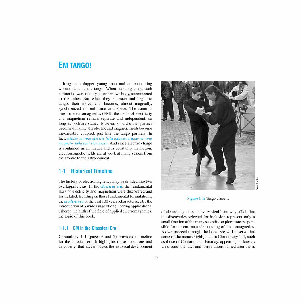
Chronology 1-2: TIMELINE FOR TELECOMMUNICATIONS

Telecommunications

1825

1837 Samuel Morse(American) patents the electromagnetic telegraph, using a code of dots and dashes to represent letters and numbers.

1872 Thomas Edison (American) patents the electric typewriter.

1876 Alexander Bell (Scottish-American) invents the telephone, the rotary dial becomes available in 1890, and by 1900, telephone systems are installed in many communities.

1887 Heinrich Hertz (German) generates radio waves and demonstrates that they share the same properties as light.

1887 Emil Berliner (American) invents the flat gramophonedisc, or record.

1893 Valdemar Poulsen(Danish) invents thefirst magnetic sound recorder using steelwire as recording medium.

Guglielmo Marconi (Italian) files his first of many patentson wireless transmission by radio. In 1901, he demonstrates radio telegraphy across the Atlantic Ocean. [1909 Nobel prize in physics, shared with Karl Braun (German).]

1897 Karl Braun (German) invents the cathode ray tube (CRT). [1909 Nobel prize with Marconi.]

1902 Reginald Fessenden (American) invents amplitude modulation for telephone transmission. In 1906, he introduces AM radio broadcasting of speech and music on Christmas Eve.

1912 Lee De Forest(American) develops the triode tube amplifier forwireless telegraphy. Also in 1912, the wireless distress call issued by the Titanic was heard 58 miles away by the ocean liner Carpathia, which managed to rescue 705 Titanic passengers 3.5 hours later.

1919 Edwin Armstong (American) invents the superheterodyne radio receiver.

1920 Birth of commercial radio broadcasting; Westinghouse Corporation establishes radio station KDKA in Pittsburgh, Pennsylvania.

1896William Sturgeon(English) develops the multiturn electromagnet.

1-2 DIMENSIONS, UNITS, AND NOTATION 9

1958 Jack Kilby (American) builds first integrated circuit (IC) on germanium and, independently, Robert Noyce (American)builds first IC on silicon.

Echo, the first passive communication satellite is launched, and successfully reflects radio signals back to Earth. In 1963, the first communication satellite is placed in geosynchronous orbit.

1969 ARPANET is established by the U.S. Department of Defense, to evolve later into the Internet.

1979 Japan builds the first cellular telephone network:• 1983 cellular phone networks start in the United States.• 1990 electronic beepers become common.• 1995 cell phones become widely available.• 2002 cell phone supports video and Internet.

1984 Worldwide Internet becomes operational.

1988 First transatlantic optical fiber cable between the U.S. and Europe.

1997 Mars Pathfinder sends images to Earth.

2004 Wireless communication supported by many airports, university campuses, and other facilities.

Vladimir Zworykin(Russian-American) invents television. In 1926, John Baird (Scottish) transmits TV images over telephone wires from London to Glasgow. Regular TV broadcastingbegan in Germany (1935), England (1936), and the United States (1939).

1926 Transatlantic telephone service between London and New York.

1932 First microwave telephone link, installed (by Marconi) between Vatican City and the Pope’s summer residence.

1933 Edwin Armstrong (American) invents frequency modulation (FM) for radio transmission.

1935 Robert Watson Watt(Scottish) invents radar.

1938 H. A. Reeves (American) invents pulse code modulation (PCM).

1947 William Schockley, Walter Brattain, and John Bardeen (all Americans) invent the junction transistor at Bell Labs. [1956 Nobel prize in physics.]

1955 Pager is introduced as a radio communication product in hospitals and factories.

1955 Navender Kapany (Indian American) demonstrates the optical fiber as a low-loss, light-transmission medium.

1923

1960

Chronology 1-2: TIMELINE FOR TELECOMMUNICATIONS (continued)

Telecommunications

10 CHAPTER 1 INTRODUCTION

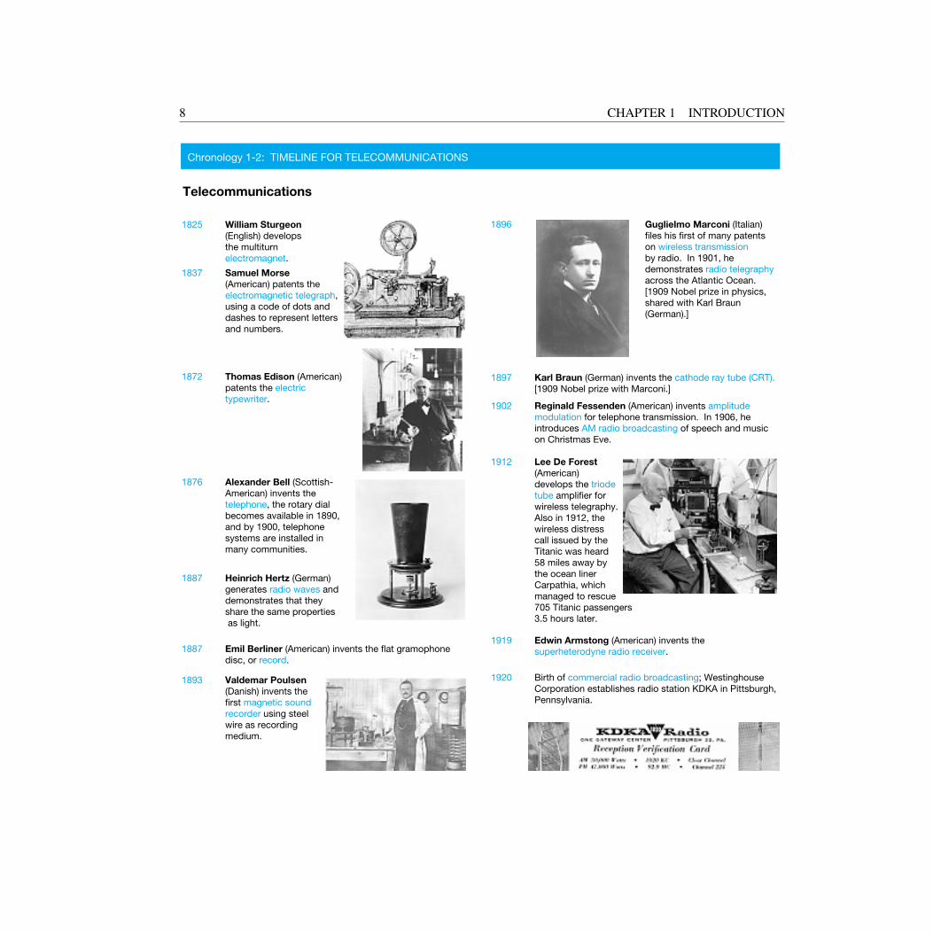
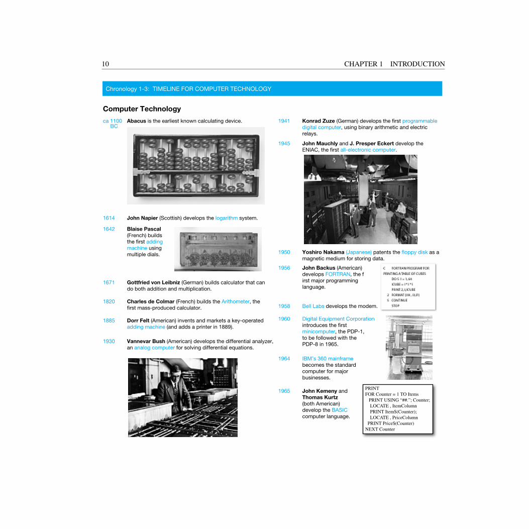
1941 Konrad Zuze (German) develops the first programmable digital computer, using binary arithmetic and electric relays.

1945 John Mauchly and J. Presper Eckert develop the ENIAC, the first all-electronic computer.

1950 Yoshiro Nakama (Japanese) patents the floppy disk as amagnetic medium for storing data.

1956 John Backus (American) develops FORTRAN, the first major programminglanguage.

1958 Bell Labs develops the modem.

1960 Digital Equipment Corporationintroduces the first minicomputer, the PDP-1, to be followed with the PDP-8 in 1965.

1964 IBM’s 360 mainframebecomes the standard computer for major businesses.

1965 John Kemeny and Thomas Kurtz(both American)develop the BASICcomputer language.

Chronology 1-3: TIMELINE FOR COMPUTER TECHNOLOGY

Computer Technology

ca 1100 Abacus is the earliest known calculating device.

1614 John Napier (Scottish) develops the logarithm system.

Blaise Pascal(French) buildsthe first addingmachine using multiple dials.

Gottfried von Leibniz (German) builds calculator that can do both addition and multiplication.

Charles de Colmar (French) builds the Arithometer, the first mass-produced calculator.

1642

1671

1820

1885 Dorr Felt (American) invents and markets a key-operated adding machine (and adds a printer in 1889).

1930 Vannevar Bush (American) develops the differential analyzer, an analog computer for solving differential equations.

BC

PRINTFOR Counter = 1 TO Items PRINT USING “##.”; Counter; LOCATE , ItemColumn PRINT Item$(Counter); LOCATE , PriceColumn PRINT Price$(Counter)NEXT Counter

1-2 DIMENSIONS, UNITS, AND NOTATION 11

Chronology 1-3: TIMELINE FOR COMPUTER TECHNOLOGY (continued)

Computer Technology

1989 Tim Berners Lee (British) invents the World Wide Web by introducing a networked hypertext system.

1991 Internet connects to 600,000 hosts in more than 100 countries.

1995 Sun Microsystems introduces the Java programminglanguage.

1996 Sabeer Bhatia (Indian American) and Jack Smith(American)launch Hotmail, the first webmail service.

1997 IBM’s Deep Blue computer defeats World Chess Champion Garry Kasparov.

1997 Palm Pilot becomes widely available.

1968

1971 Texas Instruments introduces the pocket calculator.

1971 Ted Hoff (American) invents the Intel 4004, the first computer microprocessor.

1976 IBM introduces the laser printer.

1976 Apple Computer sells Apple Iin kit form, followed by the fully assembledApple II in 1977 and the Macintosh in 1984.

1980 Microsoft introduces theMS-DOS computer disk operating system. Microsoft Windows is marketed in 1985.

1981 IBM introduces the PC.

IBM

pal

mO

ne In

c.

IBM

Ap

ple

IBM

Tom

How

e

Knn

ight

-Rid

der

Texa

s In

stru

men

ts

Douglas Engelbart (American) demonstrates a word-processor system, the mouse pointing device and the use of “windows.”

12 CHAPTER 1 INTRODUCTION

1-3 The Nature of EM

Our physical universe is governed by four fundamentalforces of nature:

• The nuclear force is the strongest of the four, but itis limited to submicroscopic systems (nuclei).

• The electromagnetic force, whose strength is onthe order of 10−2 that of the nuclear force, is thedominant force in microscopic systems, such asatoms and molecules.

• The weak-interaction force, whose strength is only10−14 that of the nuclear force, plays a role ininteractions involving radioactive particles.

• The gravitational force is the weakest of all fourforces, but it is the dominant force in macroscopicsystems, such as the solar system.

Our interest in this book is with the electromagnetic forceand its consequences, and the purpose of this sectionis to provide an overview of the basic framework ofelectromagnetism. As a precursor, however, we will takeadvantage of our familiarity with the gravitational forceby describing some of its properties because they providea useful analogue to those of the electromagnetic force.

1-3.1 The Gravitational Force: A UsefulAnalogue

According to Newton’s law of gravity, the gravitationalforce Fg21

acting on massm2 due to a massm1 at a distanceR12 from m2, as depicted in Fig. 1-2, is given by

Fg21= −R12

Gm1m2

R212

(N), (1.2)

where G is the universal gravitational constant, R12 isa unit vector that points from m1 to m2, and the unitfor force is newton (N). The negative sign in Eq. (1.2)accounts for the fact that the gravitational force isattractive. Conversely, Fg12

= −Fg21, where Fg12

is the

m1

m2

Fg12

Fg21

R12^

R12

Figure 1-2: Gravitational forces between two masses.

m1

–R

1ψψψψψψ

Figure 1-3: Gravitational field ψψψ1 induced by a mass m1.

force acting on mass m1 due to the gravitational pullof mass m2. Note that the first subscript of Fg denotesthe mass experiencing the force and the second subscriptdenotes the source of the force.

The force of gravitation acts at a distance; that is, thetwo objects do not have to be in direct contact for eachto experience the pull by the other. This phenomenon ofdirect action at a distance has led to the concept of fields.An object of mass m1 induces a gravitational field ψψψ1

(Fig. 1-3) that does not physically emanate from theobject, but its influence exists at every point in spacesuch that if another object of mass m2 were to exist at a

1-3 THE NATURE OF ELECTROMAGNETISM 13

distance R12 from object m1 then the second object m2

would experience a force acting on it equal in strengthto that given by Eq. (1.2). At a distance R from m1, thefield ψψψ1 is a vector defined as

ψψψ1 = −RGm1

R2(N/kg), (1.3)

where R is a unit vector that points in the radial directionaway from object m1, and therefore −R points toward m1.The force due to ψψψ1 acting on a mass m2 at a distanceR = R12 along the direction R = R12 is

Fg21= ψψψ1m2 = −R12

Gm1m2

R212

. (1.4)

The field concept may be generalized by defining thegravitational fieldψψψ at any point in space such that, whena test mass m is placed at that point, the force Fg actingon m is related to ψψψ by

ψψψ = Fg

m. (1.5)

The force Fg may be due to a single mass or a distributionof many masses.

1-3.2 Electric Fields

The electromagnetic force consists of an electrical forceFe and a magnetic force Fm. The electrical force Fe

is similar to the gravitational force, but with a majordifference. The source of the gravitational field is mass,and the source of the electrical field is electric charge, andwhereas both types of fields vary inversely as the squareof the distance from their respective sources, electriccharge may have positive or negative polarity, whereasmass does not exhibit such a property.

We know from atomic physics that all matter containsa mixture of neutrons, positively charged protons, andnegatively charged electrons, with the fundamentalquantity of charge being that of a single electron, usuallydenoted by the letter e. The unit by which electric chargeis measured is the coulomb (C), named in honor of the

eighteenth-century French scientist Charles Augustin deCoulomb (1736–1806). The magnitude of e is

e = 1.6 × 10−19 (C). (1.6)

The charge of a single electron is qe = −e and that ofa proton is equal in magnitude but opposite in polarity:qp = e. Coulomb’s experiments demonstrated that:

(1) two like charges repel one another, whereas twocharges of opposite polarity attract,

(2) the force acts along the line joining the charges, and

(3) its strength is proportional to the product ofthe magnitudes of the two charges and inverselyproportional to the square of the distance betweenthem.

These properties constitute what today is calledCoulomb’s law, which can be expressed mathematicallyby the following equation:

Fe21 = R12q1q2

4πε0R212

(N) (in free space), (1.7)

where Fe21 is the electrical force acting on charge q2 dueto charge q1, R12 is the distance between the two charges,R12 is a unit vector pointing from charge q1 to charge q2

(Fig. 1-4), and ε0 is a universal constant called theelectrical permittivity of free space [ε0 = 8.854 × 10−12

farad per meter (F/m)]. The two charges are assumedto be in free space (vacuum) and isolated from allother charges. The force Fe12 acting on charge q1 due tocharge q2 is equal to force Fe21 in magnitude, but oppositein direction; Fe12 = −Fe21 .

The expression given by Eq. (1.7) for the electricalforce is analogous to that given by Eq. (1.2) for thegravitational force, and we can extend the analogy further

14 CHAPTER 1 INTRODUCTION

+q1

+q2

Fe12

Fe21

R12^

R12

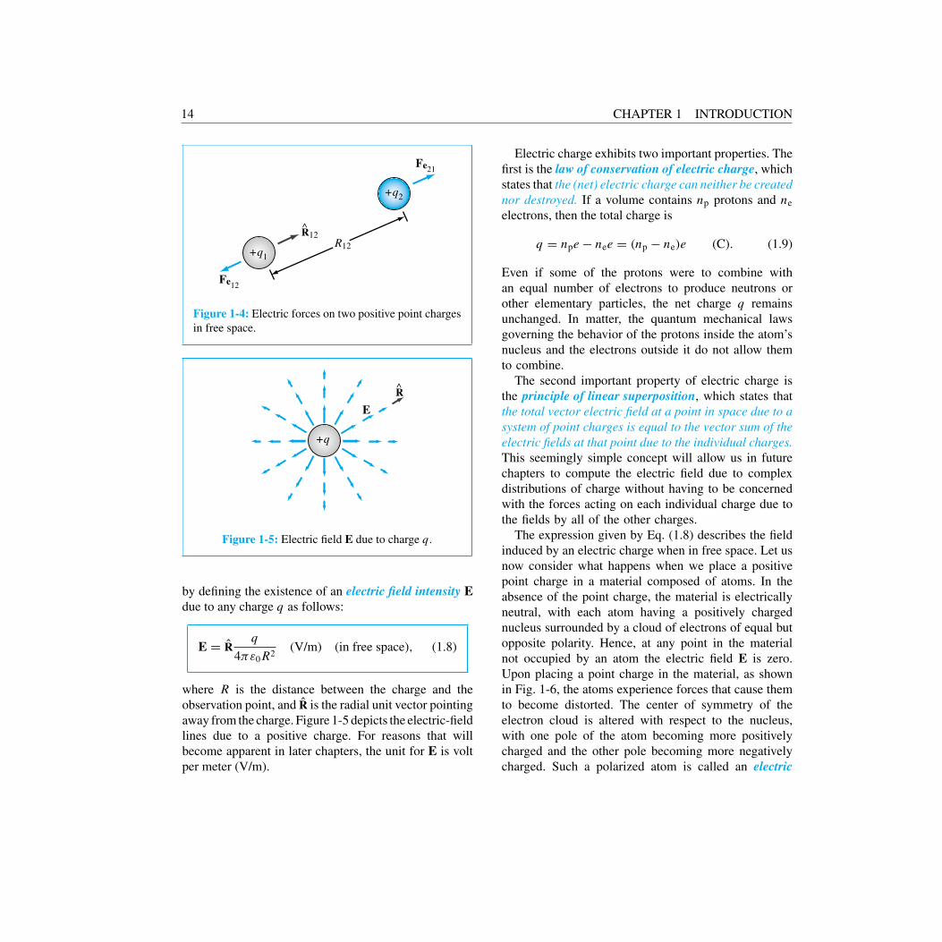
Figure 1-4: Electric forces on two positive point chargesin free space.

+q

E

R

Figure 1-5: Electric field E due to charge q.

by defining the existence of an electric field intensity Edue to any charge q as follows:

E = Rq

4πε0R2(V/m) (in free space), (1.8)

where R is the distance between the charge and theobservation point, and R is the radial unit vector pointingaway from the charge. Figure 1-5 depicts the electric-fieldlines due to a positive charge. For reasons that willbecome apparent in later chapters, the unit for E is voltper meter (V/m).

Electric charge exhibits two important properties. Thefirst is the law of conservation of electric charge, whichstates that the (net) electric charge can neither be creatednor destroyed. If a volume contains np protons and ne

electrons, then the total charge is

q = npe − nee = (np − ne)e (C). (1.9)

Even if some of the protons were to combine withan equal number of electrons to produce neutrons orother elementary particles, the net charge q remainsunchanged. In matter, the quantum mechanical lawsgoverning the behavior of the protons inside the atom’snucleus and the electrons outside it do not allow themto combine.

The second important property of electric charge isthe principle of linear superposition, which states thatthe total vector electric field at a point in space due to asystem of point charges is equal to the vector sum of theelectric fields at that point due to the individual charges.This seemingly simple concept will allow us in futurechapters to compute the electric field due to complexdistributions of charge without having to be concernedwith the forces acting on each individual charge due tothe fields by all of the other charges.

The expression given by Eq. (1.8) describes the fieldinduced by an electric charge when in free space. Let usnow consider what happens when we place a positivepoint charge in a material composed of atoms. In theabsence of the point charge, the material is electricallyneutral, with each atom having a positively chargednucleus surrounded by a cloud of electrons of equal butopposite polarity. Hence, at any point in the materialnot occupied by an atom the electric field E is zero.Upon placing a point charge in the material, as shownin Fig. 1-6, the atoms experience forces that cause themto become distorted. The center of symmetry of theelectron cloud is altered with respect to the nucleus,with one pole of the atom becoming more positivelycharged and the other pole becoming more negativelycharged. Such a polarized atom is called an electric

1-3 THE NATURE OF ELECTROMAGNETISM 15

+–

+–

+–+–+–

+–+–+–+

–

+–+–+

–+

–

+–

+–

+–

+–

+ – + – + –+

–

+ – + –

+–

+–

+–

+–

+–

+–

+–

+–

+–

+–+–+–+

–

+–+–

+–

+–

+–

+–

+–

+–

+ – + – + –+

–

+ – + –+

–+–

+–

+–

+–

+–

+–

+–

q++ – + – + – + –

Figure 1-6: Polarization of the atoms of a dielectricmaterial by a positive charge q.

dipole, and the distortion process is called polarization.The degree of polarization depends on the distancebetween the atom and the isolated point charge, andthe orientation of the dipole is such that the dipole axisconnecting its two poles is directed toward the pointcharge, as illustrated schematically in Fig. 1-6. The netresult of this polarization process is that the electricdipoles of the atoms (or molecules) tend to counteractthe field due to the point charge. Consequently, theelectric field at any point in the material would bedifferent from the field that would have been inducedby the point charge in the absence of the material.To extend Eq. (1.8) from the free-space case to anymedium, we replace the permittivity of free space ε0

with ε, where ε is now the permittivity of the materialin which the electric field is measured and is thereforecharacteristic of that particular material. Thus,

E = Rq

4πεR2(V/m). (1.10)

Often, ε is expressed in the form

ε = εrε0 (F/m), (1.11)

where εr is a dimensionless quantity called the relativepermittivity or dielectric constant of the material. Forvacuum, εr = 1; for air near Earth’s surface, εr = 1.0006;and for materials that we will have occasion to use in thisbook, their values of εr are tabulated in Appendix B.

In addition to the electric field intensity E, we will oftenfind it convenient to also use a related quantity called theelectric flux density D, given by

D = εE (C/m2), (1.12)

and its unit is coulomb per square meter (C/m2). Thesetwo electrical quantities, E and D, constitute one of twofundamental pairs of electromagnetic fields. The secondpair consists of the magnetic fields discussed next.

1-3.3 Magnetic Fields

As early as 800 B.C., the Greeks discovered that certainkinds of stones exhibit a force that attracts pieces of iron.These stones are now called magnetite (Fe3O4) and thephenomenon they exhibit is magnetism. In the thirteenthcentury, French scientists discovered that, when a needlewas placed on the surface of a spherical natural magnet,the needle oriented itself along different directions fordifferent locations on the magnet. By mapping thedirections taken by the needle, it was determined that themagnetic force formed magnetic-field lines that encircledthe sphere and appeared to pass through two pointsdiametrically opposite each other. These points, calledthe north and south poles of the magnet, were foundto exist for every magnet, regardless of its shape. Themagnetic-field pattern of a bar magnet is displayed inFig. 1-7. It was also observed that like poles of differentmagnets repel each other and unlike poles attract eachother. This attraction–repulsion property is similar to theelectric force between electric charges, except for oneimportant difference: electric charges can be isolated,but magnetic poles always exist in pairs. If a permanent

16 CHAPTER 1 INTRODUCTION

S

N

B

Figure 1-7: Pattern of magnetic field lines around a barmagnet.

magnet is cut into small pieces, no matter how small eachpiece is, it will always have a north and a south pole.

The magnetic lines encircling a magnet are calledmagnetic-field lines and represent the existence of amagnetic field called the magnetic flux density B.A magnetic field not only exists around permanentmagnets but can also be created by electric current.This connection between electricity and magnetism wasdiscovered in 1820 by the Danish scientist Hans Oersted(1777–1851), who found that an electric current in a wirecaused a compass needle placed in its vicinity to deflectand that the needle turned so that its direction was alwaysperpendicular to the wire and to the radial line connectingthe wire to the needle. From these observations, itwas deduced that the current-carrying wire induced amagnetic field that formed closed circular loops aroundthe wire, as illustrated in Fig. 1-8. Shortly after Oersted’sdiscovery, French scientists Jean Baptiste Biot and FelixSavart developed an expression that relates the magneticflux density B at a point in space to the current I in

B

BB

B^

z

y

x

r

B

BB

B

Iφφφφφ

Figure 1-8: The magnetic field induced by a steadycurrent flowing in the z-direction.

the conductor. Application of their formulation, knowntoday as the Biot–Savart law, to the situation depicted inFig. 1-8 for a very long wire leads to the result that themagnetic flux density B induced by a constant current I

flowing in the z-direction is given by

B = φφφµ0I

2πr(T), (1.13)

where r is the radial distance from the current and φφφ is anazimuthal unit vector denoting the fact that the magneticfield direction is tangential to the circle surrounding thecurrent, as shown in Fig. 1-8. The magnetic field ismeasured in tesla (T), named in honor of Nikola Tesla(1856–1943), a Croatian-American electrical engineerwhose work on transformers made it possible to transportelectricity over long wires without too much loss. Thequantity µ0 is called the magnetic permeability of freespace [µ0 = 4π × 10−7 henry per meter (H/m)], and itis analogous to the electric permittivity ε0. In fact, as wewill see in Chapter 7, the product of ε0 and µ0 specifies c,

1-3 THE NATURE OF ELECTROMAGNETISM 17

the velocity of light in free space, as follows:

c = 1√µ0ε0

= 3 × 108 (m/s). (1.14)

The majority of natural materials are nonmagnetic,meaning that they exhibit a magnetic permeabilityµ = µ0. For ferromagnetic materials, such as iron andnickel, µ can be much larger than µ0. The magneticpermeability µ accounts for magnetization properties ofa material. In analogy with Eq. (1.11), µ of a particularmaterial can be defined as

µ = µrµ0 (H/m), (1.15)

where µr is a dimensionless quantity called the relativemagnetic permeability of the material. The values of µr

for commonly used ferromagnetic materials are given inAppendix B.

We stated earlier that E and D constitute one of twopairs of electromagnetic field quantities. The second pairis B and themagnetic field intensityH, which are relatedto each other through µ:

B = µH. (1.16)

1-3.4 Static and Dynamic Fields

Because the electric field E is governed by the charge q

and the magnetic field H is governed by I = dq/dt , andsince q and dq/dt are independent variables, the inducedelectric and magnetic fields are independent of oneanother as long as I remains constant. To demonstrate thevalidity of this statement, consider for example a smallsection of a beam of charged particles that are moving ata constant velocity. The moving charges constitute a d-ccurrent. The electric field due to that section of the beam isdetermined by the total charge q contained in that section.

The magnetic field does not depend on q, but rather onthe rate of charge (current) flowing through that section.Few charges moving very fast can constitute the samecurrent as many charges moving slowly. In these twocases the induced magnetic field will be the same becausethe current I is the same, but the induced electric fieldwill be quite different because the numbers of chargesare not the same.Electrostatics and magnetostatics, corresponding to

stationary charges and steady currents, respectively,are special cases of electromagnetics. They representtwo independent branches, so characterized becausethe induced electric and magnetic fields are uncoupledto each other. Dynamics, the third and more generalbranch of electromagnetics, involves time-varying fieldsinduced by time-varying sources, that is, currents andcharge densities. If the current associated with the beamof moving charged particles varies with time, then theamount of charge present in a given section of the beamalso varies with time, and vice versa. As we will seein Chapter 6, the electric and magnetic fields becomecoupled to each other in that case. In fact, a time-varyingelectric field will generate a time-varying magnetic field,and vice versa. Table 1-3 provides a summary of the threebranches of electromagnetics.

The electric and magnetic properties of materials arecharacterized by the two parameters ε andµ, respectively.A third fundamental parameter is also needed, theconductivity of a material σ , which is measured insiemens per meter (S/m). The conductivity characterizesthe ease with which charges (electrons) can move freelyin a material. If σ = 0, the charges do not movemore than atomic distances and the material is said tobe a perfect dielectric, and if σ = ∞, the chargescan move very freely throughout the material, which isthen called a perfect conductor. The material parametersε, µ, and σ are often referred to as the constitutiveparameters of a material (Table 1-4). A medium is saidto be homogeneous if its constitutive parameters areconstant throughout the medium.

18 CHAPTER 1 INTRODUCTION

Table 1-3: The three branches of electromagnetics.

Branch Condition Field Quantities (Units)

Electrostatics Stationary charges Electric field intensity E (V/m)(∂q/∂t = 0) Electric flux density D (C/m2)

D = εEMagnetostatics Steady currents Magnetic flux density B (T)

(∂I/∂t = 0) Magnetic field intensity H (A/m)B = µH

Dynamics Time-varying currents E, D, B, and H(Time-varying fields) (∂I/∂t = 0) (E, D) coupled to (B, H)

Table 1-4: Constitutive parameters of materials.

Parameter Units Free-space Value

Electrical permittivity ε F/m ε0 = 8.854 × 10−12 (F/m)

1

36π× 10−9 (F/m)

Magnetic permeability µ H/m µ0 = 4π × 10−7 (H/m)

Conductivity σ S/m 0

REVIEW QUESTIONS

Q1.1 What are the four fundamental forces of natureand what are their relative strengths?

Q1.2 What is Coulomb’s law? State its properties.

Q1.3 What are the two important properties of electriccharge?

Q1.4 What do the electrical permittivity and magneticpermeability of a material account for?

Q1.5 What are the three branches and associatedconditions of electromagnetics?

1-4 The Electromagnetic Spectrum

Visible light belongs to a family of waves called theelectromagnetic spectrum (Fig. 1-9). Other membersof this family include gamma rays, X-rays, infraredwaves, and radio waves. Generically, they all are calledelectromagnetic (EM) waves because they share thefollowing fundamental properties:

• An EM wave consists of electric and magnetic fieldintensities that oscillate at the same frequency f .

• The phase velocity of an EM wave propagating invacuum is a universal constant given by the velocityof light c, defined earlier by Eq. (1.14).

1-4 THE ELECTROMAGNETIC SPECTRUM 19

1 fm 1 pm 1 nm1 Å

1 EHz 1 PHz 1 THz 1 GHz 1 MHz 1 kHz 1 Hz

1 µm 1 mm 1 km 1 Mm1 m

10–15

1023 1021 1018 1015 1012 109 106 103 1

10–12 10–10 10–9 10–6 10–3 103 106 1081

Frequency (Hz)

Wavelength (m)

visible

Gamma raysCancer therapy

X-rays

Medical diagnosis

Ultraviolet

Sterilization

InfraredHeating,

Night vision

Radio spectrumCommunication, radar, radio and TV broadcasting,

radio astronomy

Atmospheric opacity

100%

0

Atmosphere opaque

Opticalwindow

Infraredwindows Radio window

Ionosphere opaque

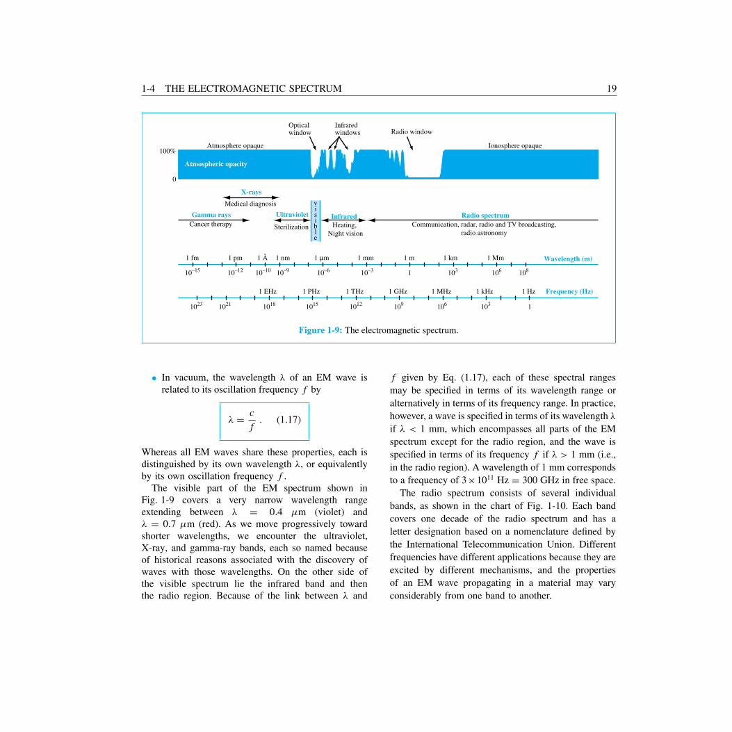
Figure 1-9: The electromagnetic spectrum.

• In vacuum, the wavelength λ of an EM wave isrelated to its oscillation frequency f by

λ = c

f. (1.17)

Whereas all EM waves share these properties, each isdistinguished by its own wavelength λ, or equivalentlyby its own oscillation frequency f .

The visible part of the EM spectrum shown inFig. 1-9 covers a very narrow wavelength rangeextending between λ = 0.4 µm (violet) andλ = 0.7 µm (red). As we move progressively towardshorter wavelengths, we encounter the ultraviolet,X-ray, and gamma-ray bands, each so named becauseof historical reasons associated with the discovery ofwaves with those wavelengths. On the other side ofthe visible spectrum lie the infrared band and thenthe radio region. Because of the link between λ and

f given by Eq. (1.17), each of these spectral rangesmay be specified in terms of its wavelength range oralternatively in terms of its frequency range. In practice,however, a wave is specified in terms of its wavelength λ

if λ < 1 mm, which encompasses all parts of the EMspectrum except for the radio region, and the wave isspecified in terms of its frequency f if λ > 1 mm (i.e.,in the radio region). A wavelength of 1 mm correspondsto a frequency of 3×1011 Hz = 300 GHz in free space.

The radio spectrum consists of several individualbands, as shown in the chart of Fig. 1-10. Each bandcovers one decade of the radio spectrum and has aletter designation based on a nomenclature defined bythe International Telecommunication Union. Differentfrequencies have different applications because they areexcited by different mechanisms, and the propertiesof an EM wave propagating in a material may varyconsiderably from one band to another.

20 CHAPTER 1 INTRODUCTION

Radar, advanced communication systems,remote sensing, radio astronomy

Extremely High FrequencyEHF (30 - 300 GHz)

Radar, satellite communication systems, aircraftnavigation, radio astronomy, remote sensing

Super High FrequencySHF (3 - 30 GHz)

TV broadcasting, radar, radio astronomy,microwave ovens, cellular telephone

Ultra High FrequencyUHF (300 MHz - 3 GHz)

TV and FM broadcasting, mobile radiocommunication, air traffic control

Very High FrequencyVHF (30 - 300 MHz)

Short wave broadcastingHigh FrequencyHF (3 - 30 MHz)

AM broadcastingMedium FrequencyMF (300 kHz - 3 MHz)

Radio beacons, weather broadcast stationsfor air navigation

Low FrequencyLF (30 - 300 kHz)

Navigation and position locationVery Low FrequencyVLF (3 - 30 kHz)

Audio signals on telephoneUltra Low FrequencyULF (300 Hz - 3 kHz)

Ionospheric sensing, electric powerdistribution, submarine communication

Super Low FrequencySLF (30 - 300 Hz)

Detection of buried metal objectsExtremely Low FrequencyELF (3 - 30 Hz)

f < 3 Hz) Magnetotelluric sensing of theearth's structure

1012

109

106

103

300 GHz

1 GHz

1 MHz

1 kHz

1 Hz

Microwave

Frequency (Hz)

Band Applications

Figure 1-10: Individual bands of the radio spectrum and their primary applications.

REVIEW QUESTIONSQ1.6 What are the three fundamental properties ofEM waves?Q1.7 What is the range of frequencies covered by themicrowave band?Q1.8 What is the wavelength range of the visiblespectrum? What are some of the applications of theinfrared band?

CHAPTER HIGHLIGHTS

• Electromagnetics is the study of electric andmagnetic phenomena and their engineering appli-cations.

• The International System of Units consists of thesix fundamental dimensions listed in Table 1-1.The units of all other physical quantities can beexpressed in terms of the six fundamental units.

CHAPTER HIGHLIGHTS 21

• The four fundamental forces of nature are thenuclear, weak-interaction, electromagnetic andgravitational forces.

• The source of the electric field quantities Eand D is the electric charge q. In a material,E and D are related by D = εE, where ε isthe electrical permittivity of the material. In freespace, ε = ε0 (1/36π) × 10−9 (F/m).

• The source of the magnetic field quantities Band H is the electric current I . In a material,B and H are related by B = µH, where µ isthe magnetic permeability of the medium. In freespace, µ = µ0 = 4π × 10−7 (H/m).

• Electromagnetics consists of three branches:(1) electrostatics, which pertains to stationaryor constant-density charges, (2) magnetostatics,which pertains to steady currents, and (3)electrodynamics, which pertains to time-varyingcurrents.

• An electromagnetic (EM) wave consists ofoscillating electric and magnetic field intensitiesand travels in free space at the velocity of lightc = 1/

√ε0µ0 . The EM spectrum encompasses

gamma rays, X-rays, visible light, infrared waves,and radio waves.