Embed Size (px)
Citation preview

Predictive Maintenance of Pumps Using Condition Monitoring
by Raymond S. Beebe
• ISBN: 1856174085
• Pub. Date: April 2004
• Publisher: Elsevier Science & Technology Books

Preface
Why yet another book on pumps? There are many excellent books on pumps, but surprisingly little has been included or published on the application of condition monitoring to these machines. After motors, pumps would be the most common machines in the world and are certainly responsible for significant consumption of energy.
I have heard and read many times of the concerns about the aging of the engineering workforce. If not already occurring, a high departure rate is imminent. With the rush to downsize, many companies have not recruited and trained new people for some time, so lots of the intellectual capital is going out the door. This is at a time when plant is being required to operate beyond the expectations of its designers, to the limits of its reliability. Work that is non-standard or out of compliance is costing industry dearly, with most of this loss due to lack of procedures and knowledge.
It is therefore vital to try and capture as much as possible of the skills and knowledge of this greying workforce. This book is one of my modest contributions to try and arrest the flow of knowledge.
Igor Karassik, the late pump guru, was often asked when a pump should be overhauled. His advice, given in many publications over the years, was that overhaul is justified when the internal clearances were twice the design value, or when effective capacity has been reduced by about 4%. But, before this guideline based on clearances can be used, the pump would need to be dismantled and measurements taken. Alternatively, prior to making the overhaul decision, the pump owner would need to correlate measured performance with as-found condition from past performance tests. The advice based on capacity reduction would need Head-Flow tests.
viii Preface
Manufacturers sometimes recommend overhaul in operating and maintenance manuals with statements as "when performance has deteriorated". Further information on how to measure the performance is often not provided, nor are the facilities to enable it to be done.
Over the last few years, I have been developing a method of using condition monitoring by performance analysis that can be used to help decide when a pump should be taken from service and overhauled. The papers I have presented have also appeared in journals and on websites, and this book came about as a result of publicity for a conference at which I presented on that topic.
I have long been involved with the development of condition monitoring in power plants, and have also been fortunate to have useful experiences with pumps. This led to presenting many short courses in Australia and overseas, and the writing of my first book, Machine condition monitoring. In 1992, I had the opportunity to join Monash University to develop and teach condition monitoring formally in their postgraduate programs in maintenance and reliability engineering. These programs are run by off campus learning for students all around the world, and I have been the Co-ordinator since 1996.
I have also taught rotodynamic machines at undergraduate level engineering for some years, which has been a valuable way of enlarging and consolidating my knowledge of pumps.
My aim is therefore to share this experience through this book, but not to duplicate material readily available elsewhere. Condition monitoring is closely related to troubleshooting of vibration and performance problems, with most of the same test and measurement methods used. I recommend that readers also obtain texts in that area. Our focus is on centrifugal pumps, as they are the most common and used in up to very large sizes. Positive displacement pumps are mentioned.
I acknowledge the inspiration I have received over the years from the many pump engineers that have written papers and books in this field, with work by many of them cited. The outstanding work of the International Pump Users Symposium run each year since 1984 by the Turbomachinery Laboratory of the Texas A&M University has also been an inspiration.
I have collected much of the material in this book over many years from conferences, meetings, plant visits and reading, well before the book

Preface ix
was conceived. I have tried to credit all sources when known. I trust that any not suitably acknowledged will forgive me in the spirit of sharing information.
Ray Beebe Monash University 2004
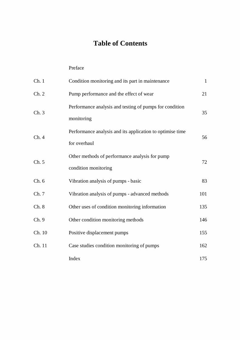
Table of Contents
Preface
Ch. 1 Condition monitoring and its part in maintenance 1
Ch. 2 Pump performance and the effect of wear 21
Ch. 3 Performance analysis and testing of pumps for condition
monitoring 35
Ch. 4 Performance analysis and its application to optimise time
for overhaul 56
Ch. 5 Other methods of performance analysis for pump
condition monitoring 72
Ch. 6 Vibration analysis of pumps - basic 83
Ch. 7 Vibration analysis of pumps - advanced methods 101
Ch. 8 Other uses of condition monitoring information 135
Ch. 9 Other condition monitoring methods 146
Ch. 10 Positive displacement pumps 155
Ch. 11 Case studies condition monitoring of pumps 162
Index 175

Cond ition mon itori ng and its part in maintenance
l The purpose of maintenance m The basic types of maintenance E The machine life cycle m Condition monitoring m The techniques of condition monitoring 11 The benefits of condition monitoring II Organising for performing condition monitoring m Leading edge maintenance management
1oi The purpose of maintenance
The fundamental purpose of maintenance in any business is to provide the required capacity for production at the lowest cost. It should be regarded as a RELIABILITY function, not as a repair function.
"Production" is the reason for an organisation existing. It is evident for process or batch production plants, but other organisations such as buildings, hospitals, the military, transport, need their own measures of output or of ongoing success, i.e. Key Performance Indicators (KPIs).
"Maintenance" work often includes major machine replacements or upgrades, which are often really capital works projects.
Reliability of a machine measures whether it does what it is required to do whenever it is required to do so. Statistically, reliability is the probability that a machine will remain on line producing as required for a desired time period. It is a function of the design on the machine (the materials used, quality of design, quality of construction) and also of the maintenance philosophy.
2 Predictive Maintenance of Pumps using Condition Monitoring
The higher the refiability, the higher the cost of making the machine and probably also of maintaining it in service. The optimum is a trade-off. In the short term, lower reliability means an increased cost of production, or an inability to meet the required demand, except maybe at greater cost. In the longer term, increased reliability and hence production can save money by deferring capital expenditure on new plant.
The fundamental purpose of maintenance can also be stated as to contribute to the production and profit objectives of the organisation by keeping plant reliability at the optimum level, consistent with safety of people and plant. Maintenance is a strategic tool for your business to gain competitive advantage. It has been stated that only 10-20% of machines reach their design life, so there is plenty of scope!
It follows that the major KPI of the success of maintenance is the extent of available production capacity which is achieved related to the cost of achieving it. Other KPIs such as the number of outstanding work requests or number of bearings used are useful but are only secondary indicators to the main aim.
In this book, we are concerned with ways of deciding which work # to be done. The skills required to do the work well are a separate act ivi ty- organisation, management, planning, leadership, equipment, workshops layout, etc. Note that it is possible to be very efficiently doing the wrong work!
Applying this philosophy to pumps is not a new idea. For many years, the late Igor Karrasik, arguably the most prominent and widely read pump engineer, responded to enquiries about pump overhauls by saying that a pump should not be opened for inspection unless either factual or circumstantial evidence indicated that overhaul is necessary (Karassik, 2001). Indications given are deterioration in performance, increased noise, or past experience with similar equipment. This book aims to assist the plant engineer in providing such information.
Io2 The basic types of maintenance
Fundamentally, it can be said that there are only two types of maintenance:
1.2.1 Breakdown maintenance
Breakdown maintenance: also known as Operate-to-failure, Corrective maintenance, repair at failure, run-to-failure.
1 �9 Condition monitoring and its part in maintenance 3
Breakdown maintenance can sometimes be cost-effective. What is the cost penalty of unexpected failure? It may be possible to increase Maintainability, such as with improved access, tools or design features to speed component changeover time and effort.
The definition of "failure" can also include "economic failure" or "economic wearout" where production continues, but at a reduced rate; or energy efficiency is reduced, such that energy consumption costs rise, or a combination of both. This is particularly relevant to pumps.
1.2.2 Preventive Maintenance
Preventive maintenance: where the plant owner decides, and takes some actions with the aim of preventing failure occurring, or at least reducing the chance of failure. There are several types:
1.2.2.1 Maintenance on fixed time or duty basis Maintenance on fixed time or duty basis (periodic preventive maintenance, fixed frequency maintenance) is usually a better way than allowing plant to fail. But, what is the optimum interval to perform it? Also, it seems strange to change parts when they look quite acceptable. Sometimes the machine doesn't go so well afterwards and we need a "post-overhaul overhaul"! The challenge is to find the correct time interval: some machines will be dismantled unnecessarily, yet others will fail because they were not inspected often enough, others will fail after maintenance work because some human-induced error has been made.
Fixed Time preventive maintenance IS effective if there is a strongly age- dependent failure mode, which is revealed by experience. There will also be routine servicing such as lubrication and adjustments that can often be done by operators (and therefore perhaps not seen as "maintenance").
Statutory inspections have long been required for some plant (e.g. pressure vessels and some underground mining plant), and are likely to extend to other types of plant as occupational health and safety focus develops and "self-regulation" extends. Usually based on fixed time intervals, the interval may be negotiable according to the engineering credibility of the plant owner.
Some plant items will not show signs of impending failure, and may never be required to perform in anger. Protection systems such as fire alarms require regular checking for reassurance.
1.2.2.2 Opportunity maintenance Opportunity maintenance takes advantage of a plant shutdown from some other cause than from the machine to be worked on. This means
4 Predictive Maintenance of Pumps using Condition Monitoring
that no production will be lost due to this machine (unless it is critical and work goes beyond the initial time window).
1.2.2.3 Design Out Maintenance Design out maintenance is an improvement s t ra tegy- redesign of a component or machine to improve performance or maintainabili ty- hopefully after the root cause of poor performance has been identified.
1.2.2.4 Management Decision Management decision: maintenance work performed for reasons other than purely economic (in the short term, at least!), such as environmental/social responsibility, corporate image, industrial relations, and local community relations.
1.2.2.5 Condition-based Maintenance Condition-based maintenance, also called predictive maintenance, condition monitoring, diagnostic testing, incipient failure detection, applies to 80% + of maintenance, according to the International Foundation for Research in Maintenance (IFIRM). Maintenance is scheduled as a result of some regular measurement or assessment of plant condition, usually trending of a parameter or parameters, and prediction of lead time to failure. The basis is that most mechanical components give some warning of their impending failure. Electronic items do however often fail suddenly.
The ultimate aim is to perform maintenance work only when it is really necessary. The old saying "If it ain't broke, don't f ix it" becomes "monitor it, and i f it is not deteriorating, leave it alone". The challenge
for the maintainer is to f ind how to monitor this inevitable deterioration reliably.
1.3 The machine life cycle
From new, or from rebuilding, machines generally show three types of failure pattern. Strictly, this behaviour pattern applies to components of machines, but if a failure mode is consistent, the pattern can be applied to the whole machine.
1.3.1 Early life
Early life, or infant mortality, is where running-in failures occur due to defects in one or more of design, manufacture, installation, commissioning and early operation, or when a machine has lots of 66 99 maintenance attention. Also known as "burn in" or "wear in" the
1 �9 Condition monitoring and its part in maintenance 5
machine becomes more reliable as operating life goes on. Quality Assurance is used in design and manufacture to try and minimise this stage.
1.3.2 Wearout
Later in life, strength of components reduces by wear, corrosion, looseness, changes in material properties or overload in service. The machine becomes less reliable with time, and eventually, wearout or breakdown occurs. The time to wearout can vary greatly, even for similar machines.
1,3.3 Useful life
Useful life occurs between the above two stages. The chance of failure is constant, and times to failure are random.
The well-known "BATH TUB" curve is a well-known model of this behaviour, and software packages (e.g. RELCODE) are available to use existing data to find which life cycle stage is being experienced. The optimum maintenance strategy for a machine will be a mixture of the approaches in 1.2 above, and is best obtained in a disciplined way, such as given by Kelly, 2000. Condition monitoring applies for the latter two life cycle stages, and is the most common outcome from RCM (Reliability Centered Maintenance) analysis (Moubray, 2001).
This requires much time and effort to do properly.
For major assets, a maintenance management system, manual or computer-based, can be set to schedule C M tests prior to scheduled overhaul. If results show that no deterioration is evident, then the maintenance work can be deferred. This process can be repeated until signs of deterioration do appear, and it is judged economic to perform the maintenance.
1.4 Condition monitoring
There are many definitions of condition monitoring, including that in Kelly, 2000. The one following emphasizes that that condition monitoring is part of maintenance, not something done by experts from outside (Beebe, 2001):
Condition monitoring, on or off-line, is a type of maintenance inspection where an operational asset is monitored and the data
6 Predictive Maintenance of Pumps using Condition Monitoring
obtained analyzed to detect signs of degradation, diagnose cause of faults, and predict for how long it can be safely or economically run.
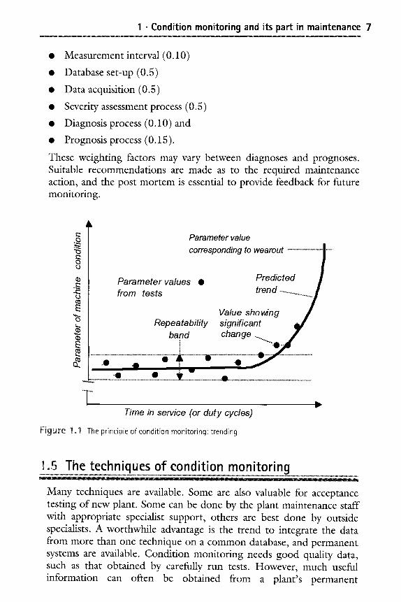
Figure 1.1 shows the basic principle. A suitable parameter is chosen that indicates internal condition of the plant item. For example, in rotating machinery, the vibration level is commonly used. Initial samples are used to establish by experience the repeatability band that is obtainable in the normal operating circumstances when the item is considered to be in good condition. Note that with new and overhauled equipment, there may be a change in measured values until the wearing-in period (infant mortality) has passed.
Routine readings are taken at suitable intervals. For most vibration monitoring, monthly is usual. For other monitoring, quarterly or even yearly is usual. Continuous monitoring may be appropriate for critical machinery. Methods for optimising inspection intervals have been developed (Sherwin and A1-Najjar, 1998). Issues such as access, size of plant and the convenience of setting up routes for data collection or testing may over-fide the theoretically ideal intervals.
When degradation eventually occurs, the parameter falls outside the repeatability band, and the frequency of readings is often increased to enable prediction of the time until the parameter corresponds to the condition where maintenance action is required. The prediction of the remaining time to failure is the most inexact part of the process, but nevertheless is usually of sufficient accuracy to meet the needs of a business. Development continues to refine this stage, e.g. ISO/ DIS13381-1, Hansen et al, 1995.
The development and application of computers to diagnose faults and assist in maintenance decision making can be expected to increase, eg Jantunen, et al, 1998; Jardine, 2000; Gopalakrishnan, 2000. The continuing development of mathematical tools (such as Barringer, 2003) to help making maintenance decisions is welcome, but these need to be very user-friendly to meet the needs of busy time-poor maintenance engineers.
ISO/DIS 13381-1 (in draft 2003) suggests an example prognosis confidence level determination, listing error sources with relative weightings"
�9 Maintenance history (0.15)
�9 Design and failure mode analysis (0.10)
�9 Analysis technique parameters used (0.15)
�9 Severity limits used (0.10)
1 �9 Condition monitoring and its part in maintenance 7
�9 Measurement interval (0.10)
�9 Database set-up (0.5)
�9 Data acquisition (0.5)
�9 Severity assessment process (0.5)
�9 Diagnosis process (0.10) and
�9 Prognosis process (0.15).
These weighting factors may vary between diagnoses and prognoses. Suitable recommendations are made as to the required maintenance action, and the post mortem is essential to provide feedback for future monitoring.
(b r (b
4:: r
E
(b E
/L
Parameter value corresponding to wearout .................... .-J .....
I Parameter values �9 Predicted from tests trend ................. . . . . /
Value showing / Repeatability significant
band change .... ~ " i ........ 'S'"
....... :~ .............. ~ .............. , ..... _ , .............. . ............... ~ .... ~ ..............
. ~ ............ : ~ .................... * ............ ~ . . . ' . ................. . ......................................................
"*'[ "o-
Time in service (or duty cycles)
Figure 1.1 The principle of condition monitoring trending
1.5 The techniques of condition monitoring
Many techniques are available. Some are also valuable for acceptance testing of new plant. Some can be done by the plant maintenance staff with appropriate specialist support, others are best done by outside specialists. A worthwhile advantage is the trend to integrate the data from more than one technique on a common database, and permanent systems are available. Condition monitoring needs good quality data, such as that obtained by carefully run tests. However, much useful information can often be obtained from a plant's permanent
8 Predictive Maintenance of Pumps using Condition Monitoring
instrumentation once repeatability is established. Advanced computer- based monitoring and control systems can often be arranged to provide condition monitoring information.
CM techniques fall into five general categories, and a machine might have one or more applied, depending on its criticality and the likely modes of degradation and the costs of failure and of monitoring. Integration of information from more than one technique is highly desirable. Several of the suppliers of vibration analysis instrumentation have extended their field into wear particle analysis, thermography and probably others. Development of data fusion systems proceed, to enable the relationship between parameters to be readily observed (Hannah et al, 2001).
1.5.1 Vibration Monitoring and Analysis
Vibration monitoring and analysis is probably the best known and most publicised technique, and the most powerful for rotating machines such as pumps. It seems logical that well-aligned and smoother running machines should use less energy and in general will also cost less to maintain (see Chapter 7).
Balancing is a common solution, temporary or permanent, to high vibration. Vibration instrumentation can usually also be used for balancing, but simpler methods are sometimes possible and acceptable (Beebe, 2001).
Useful results can be obtained with low-cost read-only instruments, but for large plants it is much more productive to use portable data collector/analysers and computer processing systems. Several good systems are available, usually with diagnostic aid software. These continue to improve in capability.
Permanent on-line monitoring systems may be cost-effective, especially where access is restricted or hazardous to people. Some consider that 10 to 20% of a plant's machines are critical enough to justify permanent systems. Data links allow experts remote from the site to access information directly. Information can also be shared throughout a company via its intranet.
Vibration standards are commonly included in specifications for rotating machinery. The site measurements taken for initial acceptance can be the start of routine measurements, and should also be part of post-maintenance quality checking.
1 �9 Condition monitoring and its part in maintenance 9
1.5.2 Visual Inspection and Non-Destructive Testing
Visual inspection and non-destructive testing usually requires the plant out of service. NDT is a well known specialist field with formal operator training and certification. The techniques are covered by several national Standards. Quality systems are thus readily applied. Visual inspection, with a range of devices from mirrors to micro TV cameras, can access through available ports but it can be worth designing special access features into the machine. Infra-red thermal imaging or Thermography is a powerful technique which fits into this grouping.
1.5.3 Performance Monitoring and Analysis
Performance monitoring and analysis is less well known, yet where deterioration in the condition of a machine results in an increase in energy usage, it is possible to calculate the optimum time to restore performance (for minimum total cost per time period). We shall examine how this applies to pumps later.
Application and parameters are developed for each type of machine or plant item, and usually require measurement of quantifies such as temperature, pressure, flow, speed, and displacement. Expedient methods of measurement and/or permanent plant instrumentation and data processing equipment can sometimes be used if repeatability of the monitoring parameters is proven to be narrow enough.
Performance parameters can also be stored and trended using the same software as supplied for vibration monitoring and analysis. Spreadsheets with charting are suggested as a simple way. If the range of the time scale is entered into the time column, (or row) as well beyond the time to date, then new data points will be automatically added to the trend chart as they are entered in the spreadsheet.
1.5.4 Analysis of wear particles in lubricants and of contaminants in process fluids
Analysis of wear particles in lubricants and of contaminants in process fluids gives more advanced warning (i.e. longer lead time) than most other predictive methods. No single analysis technique provides all the diagnosis possible, and critical machines may justify the use of more than one technique. Simply applied screening techniques are available integrated with vibration analysis, and give a quick on site assessment.
10 Predictive M
aintenance of Pumps using C
ondition Monitoring
o%
U3
E
4.a
O
qJ
c-
~> ~J ~
J
~-
O
co
c- ~-~
~J 4.u ~
J
E ~
- q
j c0 C
L
q3
s L/3
E
o o_ ~:
E
o
E
o
0 0 ~4
0 o x �9 ,..,..
Q_
E
L/3
L/3
&
t- "c
-
L/3
L/3
c-
u3
G
J -O
CL
E
CL
O
.E
O
r r co
c13 4
- c
-
~J
c-
co
c
- cJ
r ~J
E
co
co
o_
O
cJ cJ O
E c
o
c-
E O
cL
E
L/3
1 �9 Condition monitoring and its part in maintenance 1 1
1.5.5 Electrical plant testing
Electrical plant testing for low voltage machines is well known, but specialist techniques are required for high voltage plant. The main concern is evaluation of the condition of insulation, but monitoring of mechanical condition is also applicable. Devices are available for permanent installation on pumps that automatically test motor insulation, flow rate, and log the data. (MultiTrode, 2003)
1.5.6 More information about CM
Moubray (2001) gives an excellent listing of most of the techniques available for condition monitoring and their salient characteristics. Details of CM application are given in the many books and regular conference proceedings available (e.g. Rao, 1997; COMADEM, MARCON, etc.), and the new ISO Standards that are being developed and progressively released.
I~ The benefits of condition monitoring
The condition monitoring approach has become so well accepted by many companies and industries that it is now embedded into company culture and some long term users no longer bother to determine their costs and benefits. It is suggested that such an assessment should be done yearly on a sampling basis, to provide ongoing evidence of the value of the approach to the business. This gives personal satisfaction, and also ensures continuation in the event of a change in management to one with a crude cost-cutting style.
A simple case by case procedure is suggested here for determination of costs/benefits. Many find that the accumulated savings are so large that the process need not be done for every occasion, and keeping score for a sample period may be sufficient.
A. What actually happened: �9 Deterioration is detected and repairs scheduled. �9 The total cost of labour, materials, lost production, etc. is
readily found
B. What was most likely to have happened if the problem went undetected? �9 The worst case scenario should not be assumed. A refinement is
to estimate under three headings: Catastrophic, Moderate, Loss
12 Predictive Maintenance of Pumps using Condition Monitoring
of performance (noticed by operators), with appropriate estimates and probabilities.
�9 The likely total cost is estimated for labour, materials, lost production for the repairs.
The savings for this case are then found by subtracting A from B.
To find the net savings over a period, subtract the cost of running the CM activities; the annual capital cost of equipment, cost of services, people and training.
The Return on Investment can then be calculated:
Estimated total savings- Cost of running CM activities Cost of running CM activities x 100%
If the savings look unreasonably huge (and may therefore be regarded as unrealistic) a probability factor can be applied. When justifying intro- duction of condition monitoring, it is suggested that the likely probability of success be considered.
�9 If a condition monitoring technique when expertly applied is considered to be, say, 80% successful in detecting an incipient fault, and
�9 Adoption of this technique by your own people is, say, 75% of its potential, then
�9 The overall probability of achieving initial success is the product of these: i.e. 0.75 x 0.8 = 0.6 or 60% and can be fairly applied to your estimate of past losses. It is easy to derive very large potential theoretical benefits that look suspect just because they are so large.
More examples of benefits, and hints on applying condition monitoring, are given in Beebe, 1999.
One point of particular note is for condition monitoring practitioners to report their findings and recommendations simply and clearly to asset owners in an executive summary, and leave the technical details to later parts of a report or plant history file. Too often, the experts provide a learned treatise, when the asset owner just wants to know if any maintenance action is needed, when it is required to be done, and the implications if the recommendations are not followed.
1.6.1 CM for pumps
Rajan (1999 and 2002) gives an interesting approach based on evaluation of experience with pumps and other machines in the pharmaceutical industry. A spreadsheet workbook tool "Ruby" has been developed to help plant engineers evaluate quickly the viability of
1 �9 Condition monitoring and its part in maintenance 13
any type of condition Roylance, 1999).
monitoring to their situation (Rajan and
1.70rganising for performing condition monitoring
As with much engineering work, there is no single fight way to conduct condition monitoring work. The decision in any case will depend on company size and philosophy. Utilisation may be insufficient to justify owning the expensive equipment required by some techniques. Some require licensed operators, some are best done by specialists. Condition monitoring is not an end in itself, and should be managed or at least reviewed regularly by a reliability engineer to ensure that routines continue to meet business needs, and that findings lead to re-design where appropriate.
Training is available in techniques such as Root Cause Analysis that provide skills in reliability improvement, and search of the Internet will reveal many training programs and short courses in most areas of condition monitoring. In the vibration analysis field, CD-based programs are available. One can provide its signals to an analyser for training purposes on the instrumentation used by the student (iLearnInteractive).
Certification of CM practitioners is available in various technologies. Earlier work by the Vibration Institute has been considered in the ISO Standard under development (ISO18436-2:2003), and a similar approach is likely in other CM technologies.
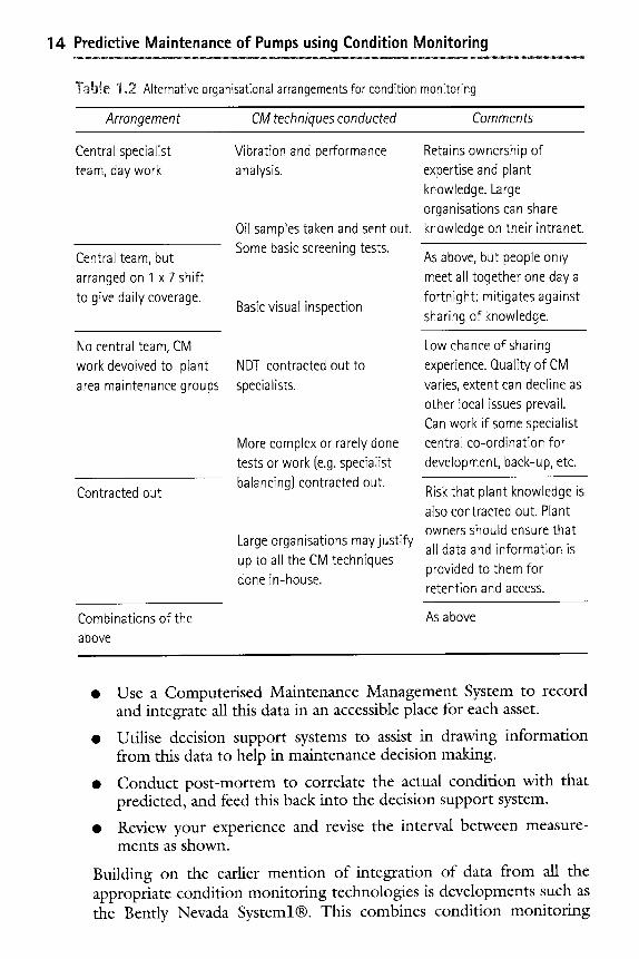
Table 1.2 on page 14 gives some alternatives arrangement for consideration.
of organizational
1.8 Leading edge maintenance management
There are many opinions on how maintenance should be decided, organized and managed, as a glance at the contents of the many books and regular conferences in this field will show. The following is offered as a contribution to the engineering component of this activity:
Decide maintenance strategy using a systematic approach, such as RCM, PMO, etc. Apply the mathematical tools of reliability engineering appropriately.
Apply one or more of the techniques of condition monitoring to the extent justified by each plant item's criticality to the business (note this is not necessarily related to the size of an item).
14 Predictive Maintenance of Pumps using Condition Monitoring
Table 1.2 Alternative organisational arrangements for condition monitoring
Arrangement CM techniques conducted Comments
Central specialist team, day work
Central team, but arranged on I x 7 shift to give daily coverage.
No central team, CM work devolved to plant area maintenance groups
Contracted out
Vibration and performance Retains ownership of analysis, expertise and plant
knowledge. Large organisations can share
Oil samples taken and sent out. knowledge on their intranet. Some basic screening tests.
As above, but people only meet all together one day a fortnight: mitigates against
Basic visual inspection sharing of knowledge.
NDT contracted out to specialists.
More complex or rarely done tests or work (e.g. specialist balancing) contracted out.
Large organisations may justify up to all the CM techniques done in-house.
Low chance of sharing experience. Quality of CM varies, extent can decline as other local issues prevail. Can work if some specialist central co-ordination for development, back-up, etc.
Risk that plant knowledge is also contracted out. Plant owners should ensure that all data and information is provided to them for retention and access.
Combinations of the As above above
�9 Use a Computerised Maintenance Management System to record and integrate all this data in an accessible place for each asset.
�9 Utilise decision support systems to assist in drawing information from this data to help in maintenance decision making.
�9 Conduct post-mortem to correlate the actual condition with that predicted, and feed this back into the decision support system.
�9 Review your experience and revise the interval between measure- ments as shown.
Building on the earlier mention of integration of data from all the appropriate condition monitoring technologies is developments such as the Bently Nevada System1| This combines condition monitoring

1 �9 Condition monitoring and its part in maintenance 1 5
data, from permanent and/or portable instruments, decision support systems, and a plant's CMMS.
The benefits of condition m o n i t o r i n g (CM)
�9 CM gives early detection of wearout/damage (in most cases)
II Better prediction of maintenance requirements
�9 Also, many small faults are detected early when "CM people" methodically tour the plant. This very act picks up developing faults which would otherwise go unnoticed.
�9 CM minimises unnecessary shutdown and opening up of plant
�9 Condition-based approach is the most common outcome from Reliability- Centred Maintenance analysis
�9 Machines are bought to make product, not to be pulled apart"
�9 Higher uptime, so less lost production and greater profit potential
�9 Less maintenance workload - but CM work does require effort (on-line monitoring may be cost-effective)
�9 More satisfying work for maintainers, less effect of errors because of direct feedback on quality of work
�9 Use CM to defer major intended work (but not all maintenance can be put off indefinitely)
II "Judicious use of CM can yield 10 to 20 times the initial outlay within the first year" - UK Dept Trade 8 Industry Report, "Maintenance into the late 19905"
�9 CM gives reassurance of safe continued operation (and is very effective when "nursing on" plant to a suitable maintenance opportunity)
�9 Cause of a problem can't be diagnosed initially? - can often eliminate some causes which have disastrous consequences: the "IS" or "IS NOT" approach (Kepner-Tregoe~)
�9 CM saves costs - reduced spares usage, maybe lower insurance premiums.
�9 Energy savings from smoother machines (e.g. alignment claimed in some cases, 3% to 5%; balancing 1% - 2%)
�9 Energy savings from scheduling overhaul to restore lost performance at optimum time
�9 CM improves product quality, customer relations, plant design, company efficiency (even ensures company survival!)
16 Predictive Maintenance of Pumps using Condition Monitoring
References
Barringer, P (2003) Predict future failures from your maintenance records MESA Speaker's Tour 2003 www.barringerl.com [Paper]
Beebe, RS (2001) Machine condition monitoring MCM Consultants 2001 reprint [ Book]
Beebe, RS (1999) Economic justification of condition monitoring Proceedings Maintenance and Reliability Conference MARCON99, Tennessee May, pp 11.01 - 11.08 [Paper]
COMADEM- Proceedings of the Conference on Diagnostic Engineering Management (annual event) [Book]
Gopalakrishnan, S (2000) Software based diagnosis of feed pump problems Proceedings MARCON 2000, Knoxville [Paper]
Hannah, P; Starr, A, Bryanston-Cross, P (2001) Condition monitoring and diagnostic engineering- a data fusion approach Proceedings of 14th International Congress of COMADEM, Elsevier [Book]
Hansen, RJ, Hall, DL, and Kurtz, SK (1995) A new approach to the challenge of machinery prognostics ASME Paper 94-GT-3. Journal of Engineering for Gas Turbines and Power April, pp 320-5 [Paper]
ISO 17359 (2003) Condition monitoring and diagnostics of machines-general guidelines [Standard]
ISO/DIS13381 -1 (2003) Condition monitoring and diagnostics of machines - Prognostics- Pt 1 General guidelines [Draft Standard]
ISO/FDIS 13379 (FDIS 2003) Condition monitoring and diagnostics of machines- General guidelines on data interpretation and diagnostics techniques [Final Draft Standard]
ISO/FDIS 13380:2003 (2003) Mechanical vibration - Condition monitoring and diagnostics of machines- General guidelines on using performance parameters [Final Draft Standard]
ISO/FDIS 18436-2:2003 (2003) Condition monitoring and diagnostics of machines - Requirements for training and certification of personnel - Part 2: Vibration condition monitoring and diagnostics [Final Draft Standard]
Jantunen, Errki et al (1998) Flexible expert system for the diagnosis of centrifugal pumps Proceedings of COMADEM 98, 11th International Conference on Condition Monitoring and Diagnostic Engineering Management pp 433-442 [Paper]
Jardine, A and Campbell, J (2000) Proportional Hazards Modeling Chapter 12 in Maintenance excellence - optimizing equipment life cycle decisions. (RELCODE and EXAKT: www.oliver-group.com/html/exakt-features.shtml)

1 �9 Condition monitoring and its part in maintenance 17
Karassik, IJ et al (Ed) (2001) Pump Handbook McGraw-Hill 3rd Edition. [Book]
Kelly, T (1997) Business Centered Maintenance Conference Communications, UK [Book]
Moubray, J (2001) Reliability Centered Maintenance Aladon [Book]
MultiTrode: www.multitrode.com.au [Website]
Rajan, BS (1999) Method of evaluating cost benefits of CBM prior to implementation of a condition monitoring strategy Reliability magazine Aug, pp 4-10
Rajan, BS (2002) Condition monitoring experience in the pharmaceutical industry and an econometric model Chapter 6 in Condition Monitoring Engineering the Practice PEP, London [Book]
Rajan, BS and Roylance, BJ (1999) Ruby - an effective way to assess the cost benefits from employing condition monitoring equipment in the maintenance of batch process plant machinery Condition Monitoring 99, Swansea [Paper]
Rao, BKN (1997) Handbook of condition monitoring Elsevier [Book]
Sherwin, DJ and A1-Najjar, B (1998) Practical models for condition monitoring inspection intervals Proceedings of ICOMS98 International Conference of Maintenance Societies, Adelaide and in Journal of Quality in Maintenance Engineering, Vol 5, No.3, 1999, pp 203-220 MCB University Press [Paper]
www. b ently, com/ar ticles/2003 ORB IT/Syste m I .pdf
Bibliography and other r e s o u r c e s
In addition to the above referenced in this chapter, these resources are suggested for further reading. This is not intended to be a complete list of every information resource, but should be enough to provide something for everyone!
Books
Bachus, L and Custodio, A (2003) Know and understand centrifugal pumps Elsevier, UK
Bently, DE and Hatch, CT, Ed Grissom, R Fundamentals of rotating machinery diagnostics Bently Pressurized Bearing Press, Minden, 2002
Bloch, HP et al Practical Machinery Management for Process Plants Gulf, 1982, etc. (Four volumes).
Crawford, Art The simplified handbook of vibration analysis (2 vols) CSi 1992
1 8 Predictive Maintenance of Pumps using Condition Monitoring
Davies, A (ed) Handbook of condition monitoring : techniques and methodology London, Chapman & Hall, 1996.
Eisenmann, RC Sr and Eisenmann, RC Jr Machinery malfunction diagnosis and correction Prentice-Hall, 1997.
Gill, P Electrical power equipment maintenance and testing Marcel Dekker 1997
Hunt, TM Condition Monitoring of Mechanical and Hydraulic Plant Chapman & Hall 1996
Idhammar, T et al Preventive maintenance, essential care and condition monitoring Idhammar 1999.
Idhammar, T Condition monitoring standards, Volumes I, II, III 2001
Jones, M H and Sleeman, DG (Ed) Condition Monitoring "99 :proceedings of an International Conference on Condition Monitoring held at University of Wales, Swansea, UK, Coxmoor Publishing, 1999.
Mitchell, JS Introduction to Machinery Analysis and Monitoring PennWell (1993)
Mobley, K: Introduction to Predictive Maintenance Technology for Energy 1991
Neale, M A Guide to Condition Monitoring of Machinery London, HMSO 1979
Palgrave, R Troubleshooting centrifugal pumps and their systems Elsevier, London 2003.
Rao, BKN Handbook of Condition Monitoring Elsevier 1997
Tavner, P J & Penman, J: Condition Monitoring of Electrical Machinery Wiley
Taylor, James The vibration analysis handbook Vibration Consultants Inc 1994
Williams, J and Davies, A Condition-based maintenance and diagnostics Chapman & Hall 1994
Wowk, V Machinery Vibration -Measurement and Analysis McGraw-Hill, 1991
All the ISO Standards in this field, as they become available.
Journals and Technical magazines and their websites (some have bulletin boards)
�9 Hydrocarbon Processing (www.hydrocarbonprocessing.com)
�9 Inmotion (www.inmotiononline.com.au)
�9 Journal of Quality in Maintenance Engineering
�9 Maintenance and Asset Management
�9 Maintenance Journal (www.maintenancejournal.com.au)

1 �9 Condition monitoring and its part in maintenance 19
�9 Maintenance Technology (www.mton-line.com)
�9 Orbit (www.bently.com)
�9 Plant Services (www.plantservices.com)
�9 Power (www.platts.com/engineering)
�9 Pumps and Systems (www.pump-zone.com)
�9 Pumps=pompes=pumpen
�9 Reliability (www.reliability-magazine.com)
�9 Sound and 18bration (www.sandv.com)
�9 WorldPumps (www.worldpumps.com)
The relevant journals of the Institution of Mechanical Engineers and the American Society of Mechanical Engineers sometimes have papers in this area.
The publishers of some of the journals mentioned above also conduct conferences. Here are some others, often with published proceedings in book form:
�9 Society of Maintenance and Reliability Professionals (www.smrp.org)
�9 Vibration Institute (www.vibinst.org) and magazine ISbrations
�9 Machinery Failure Prevention Technology Society (MFPT Society).
�9 ICOMS (International Conference of Maintenance Societies) (www.mesa.org.au)
�9 COMADEM (Conference on Monitoring and Diagnostic Engineering Management)
�9 ACSIM (Asia-Pacific Conference of Systems Integrity and Maintenance)
�9 MARCON (Maintenance and Reliability Conference) (MRC, University of Tennessee)
Websites
There are many websites: the listing in Table 1.3 is far from exhaustive. Changes occur, so a web search is suggested, using keywords such as "condition monitoring" "reliability engineering" "pumps" etc. Manufacturers of CM equipment often include application notes, and some such sites are included.

2 0 Predictive Maintenance of Pumps using Condition Monitoring
Table 1 o3 Some websites for more information on condition monitoring
Reliabilityweb.com
reliability-magazine.com
plantmaintenance.com
noria.com
http://www.skfcm.com/
inside.co.uklpwe
globalmss.com/Publications/CBM.htm
web.u kon line.co.u k/d.stevens2
coxmoor.com
mimosa.com
ndt.net
bindt.org
predict-dli.com
Pumpzone.com
plan tservices.co m
pacsciinst.com
main tena nce resou rces.co m
svdinc.com
goldson.freeon I i n e.co. u k
vibrotech.com
machinemonitor.com
pdma.com
a pt.tech nology.com.a u
www.pru ftech n i k.co.u k
mton-line.com
Pumplearning.org
snellinfrared.com
h ttp ://www.a n im a ted so ftwa re.co m / P u m pg los/p u m pg los. h tm
h ttp ://www.m cn a I lyi nsti t u te.co m/h o m e- h tm I/Web_l i n ks.h tml
bton.ac.uklengineeringlresearchlcondmonlcondmon.htm
Pump performance and the effect of w e a r
i Pump performance characteristics I Effects of internal wear on pump performance m Relationship between internal wear and efficiency m Rate of wear
Pump selection reliability factors E Case studies in detected performance shortfall
2oi Pump performance characteristics
The four basic quantifies in pump performance are Head, Power, Efficiency and Flow. A thorough explanation is given in any general pump textbook, and some are listed at the end of this chapter. Table 2.1 shows the terms, symbols and units used in this book. It is generally desirable to use manometric terms for Head, and Volumetric terms for flow. This is because the same Head-Flow curve applies for liquids at a range of temperatures (neglecting the effects of viscosity). The Power- Flow curve will change in direct proportion to liquid density. In the case of boiler feed pumps, it is customary to use pressure units and mass flow, and both Head and Power curves will change if density changes.
Usually, Head, Flow and Power are measured and Efficiency is calculated from this fundamental equation (but efficiency can be measured directly, as will be seen later)"
(Pump power output) (Pump power input)
With consistent SI units (m3/s, m, W shown in bold in Table 2.1) and bringing in g (usually 9.81 m/s2/, and the fluid density (kg/m3), with Efficiency as a decimal, this equation becomes:
22 Predictive Maintenance of Pumps using Condition Monitoring
Table 2.1 Fundamental terms and units in pump performance
Quantity Other terms used Symbol Units Other units
F l o w Volumetric flowrate, Q m3/s, L/s, m3/h, IGPM Capacity, Discharge, ML/d USGPM (1 US Quantity Sometimes kg/s gallon = 3.785L)
Head Total Head, H m, kPa Bars, ft, psi Total Dynamic Head, Generated Pressure, Generated Head
Power Power absorbed P W, kW hp
Efficiency ~I Decimal %
q ~ _ . Q g/4
P
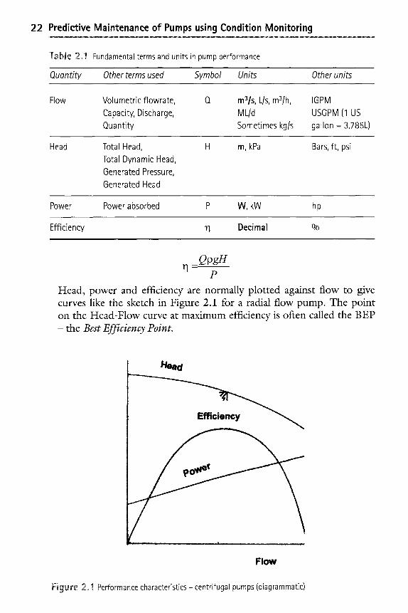
Head, power and efficiency are normally plotted against flow to give curves like the sketch in Figure 2.1 for a radial flow pump. The point on the Head-Flow curve at maximum efficiency is often called the B EP - the Best Efficiency Point.
Flow
Figure 2, I Performance characteristics - centrifugal pumps (diagrammatic)
2 �9 Pump performance and the effect of wear 23
As will be seen in any pump textbook (e.g. Stepanoff, 1957; Karassik and Grieve, 1998) the shapes of the performance curves vary with the type of impeller. Specific Speed is a dimensionless type number used to express this family relationship. It is calculated with best efficiency point data, using appropriate units. As most pump textbooks use US units with useful data and charts, use of the following metric units results in a number that is sufficiently close for the purposes of this book:
NS m ~ N4-r HO.75
where"
N = rotation speed of pump, r /min; Q = flow per impeller eye (i.e. half total flow for double
suction impellers), m3/h; H = head per stage, m
Specific Speed values calculated with these units indicate the type of pump, but the boundaries do overlap"
�9 500 to 2000" Radial impellers. (Fairly flat Head/Flow curves, rising Power curve)
�9 2000 to 8000- Mixed flow impellers. (Steeper Head/Flow curve, less steep Power curve)
�9 8000 to 16500" Axial flow impellers. (Steep Head/Flow curve, falling Power curve, sometimes with a "bump" in it)
Specific Speed can also be obtained in other metric terms. If standard SI units (rad/s, m3/s, m) are used, the resulting numbers for the categories above are: 0.2 - 1.8; 1.8 - 3.0; 2.8 - 8.0 from this equation"
N4F Ns-- (gH) ~
With other SI units (r /min, m3/s, m) the numbers are 12 to 35; 35 to 160; and 160 to 400+
Side-channel pumps have a star or vane wheel impeller of straight radial vanes without shrouds. Liquid is transferred to a side channel arranged next to the impeller. The head generated is 5 to15 times greater than that generated by a radial impeller of the same size and speed (KSB, 1990). With specific speeds between 550 and 1700, they have self- priming capability, but their relatively low efficiency limits their size to about 4kW.
24 Predictive Maintenance of Pumps using Condition Monitoring
2,2 Effects of internal wear on pump performance
The extent to which internal wear can be tolerated varies with the type of pump and the characteristics of the system in which it is installed. Slurry pumps are designed to cope with erosive liquids, wear is increased by high velocity, large solids size and high concentrations (Addie et al, 1996).
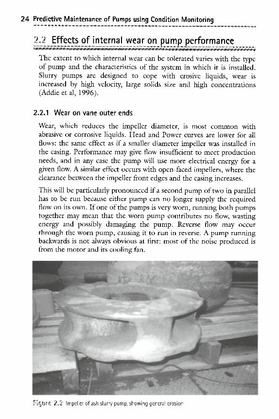
2.2.1 Wear on vane outer ends
Wear, which reduces the impeller diameter, is most common with abrasive or corrosive liquids. Head and Power curves are lower for all flows: the same effect as if a smaller diameter impeller was installed in the casing. Performance may give flow insufficient to meet production needs, and in any case the pump will use more electrical energy for a given flow. A similar effect occurs with open-faced impellers, where the clearance between the impeller front edges and the casing increases.
This will be particularly pronounced if a second pump of two in parallel has to be run because either pump can no longer supply the required flow on its own. If one of the pumps is very worn, running both pumps together may mean that the worn pump contributes no flow, wasting energy and possibly damaging the pump. Reverse flow may occur through the worn pump, causing it to run in reverse. A pump running backwards is not always obvious at first: most of the noise produced is from the motor and its cooling fan.
Fig"re 2 ~ ~...~ ,.e:.-o Impeller of ash slurry pump, showing general erosion
2 �9 Pump performance and the effect of wear 25
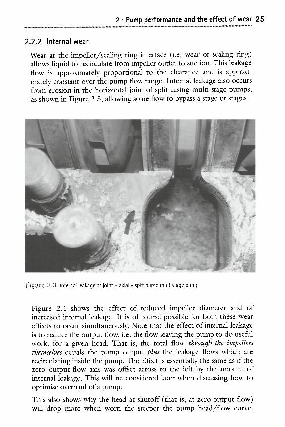
2.2.2 Internal wear
Wear at the impeller/sealing ring interface (i.e. wear or sealing ring) allows liquid to recirculate from impeller outlet to suction. This leakage flow is approximately proportional to the clearance and is approxi- mately constant over the pump flow range. Internal leakage also occurs from erosion in the horizontal joint of split-casing multi-stage pumps, as shown in Figure 2.3, allowing some flow to bypass a stage or stages.
~,gu~e 2~ Internal leakage at joint - axially split pump multistage pump
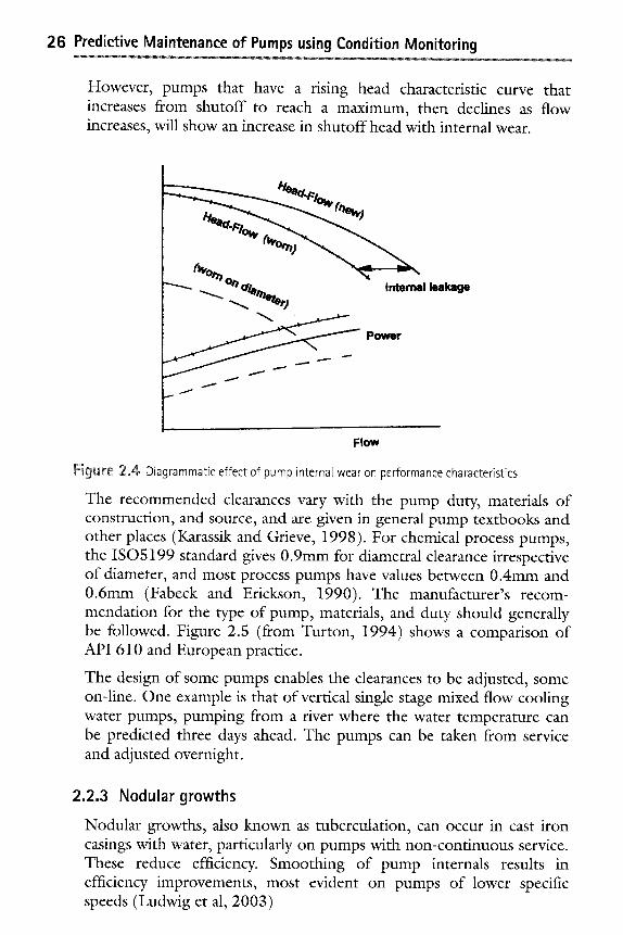
Figure 2.4 shows the effect of reduced impeller diameter and of increased internal leakage. It is of course possible for both these wear effects to occur simultaneously. Note that the effect of internal leakage is to reduce the output flow, i.e. the flow leaving the pump to do useful work, for a given head. That is, the total flow through the impellers themselves equals the pump output plus the leakage flows which are recirculating inside the pump. The effect is essentially the same as if the zero output flow axis was offset across to the left by the amount of internal leakage. This will be considered later when discussing how to optimise overhaul of a pump.
This also shows why the head at shutoff (that is, at zero output flow) will drop more when worn the steeper the pump head/f low curve.
26 Predictive Maintenance of Pumps using Condition Monitoring
However, pumps that have a rising head characteristic curve that increases from shutoff to reach a maximum, then declines as flow increases, will show an increase in shutoff head with internal wear.
J J
Internal leakage
Power
Flow
Figure 2,~4 Diagrammatic effect of pump internal wear on performance characteristics
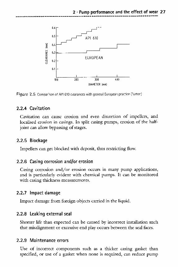
The recommended clearances vary with the pump duty, materials of construction, and source, and are given in general pump textbooks and other places (Karassik and Grieve, 1998). For chemical process pumps, the ISO5199 standard gives 0.9mm for diametral clearance irrespective of diameter, and most process pumps have values between 0.4mm and 0.6mm (Fabeck and Erickson, 1990). The manufacturer's recom- mendation for the type of pump, materials, and duty should generally be followed. Figure 2.5 (from Turton, 1994) shows a comparison of API 610 and European practice.
The design of some pumps enables the clearances to be adjusted, some on-line. One example is that of vertical single stage mixed flow cooling water pumps, pumping from a river where the water temperature can be predicted three days ahead. The pumps can be taken from service and adjusted overnight.
2.2.3 Nodular growths
Nodular growths, also known as tuberculation, can occur in cast iron casings with water, particularly on pumps with non-continuous service. These reduce efficiency. Smoothing of pump internals results in efficiency improvements, most evident on pumps of lower specific speeds (Ludwig et al, 2003)
2 �9 Pump performance and the effect of wear 27
0.6
0.5
"E 0.~ E
k~
0.3 Z < eY
" ' 0.2 _.t
0 . t -
_ j - - - -
F - F - -
I - -
API 610 F ' - -
F - -
I I . . . . . . . .
EUROPEAN
, ! I . . . . . . . . I ....
100 zoo 300 400 DIAMETER (ram)
Figure 2,5 Comparison of API 610 clearances with general European practice {Turton)
2.2.4 Cavitation
Cavitation can cause erosion and even distortion of impellers, and localised erosion in casings. In split casing pumps, erosion of the half- joint can allow bypassing of stages.
2.2.5 Blockage
Impellers can get blocked with deposit, thus restricting flow.
2.2.6 Casing corrosion and/or erosion
Casing corrosion and /o r erosion occurs in many pump applications, and is particularly evident with chemical pumps. It can be monitored with casing thickness measurements.
2.2.7 Impact damage
Impact damage from foreign objects carried in the liquid.
2.2.8 Leaking external seal
Shorter life than expected can be caused by incorrect installation such that misalignment or excessive end play occurs between the seal faces.
2.2.9 Maintenance errors
Use of incorrect components such as a thicker casing gasket than specified, or use of a gasket when none is required, can reduce pump
28 Predictive Maintenance of Pumps using Condition Monitoring
performance by introducing excess clearances inside a pump or insufficient nip on bearing shells. Rotation in reverse can occur with dc pumps if wiring leads are reversed. The pump stills pumps liquid, but the head-flow performance is well down. Double entry impellers have been mounted in reverse, such that the vanes become forward-curved and a different head-flow performance results. Impellers of the wrong size can be fitted. This is easily done, particularly if the shrouds are the expected diameter, but the vanes have been trimmed.
2,3 Relationship between internal wear and efficiency
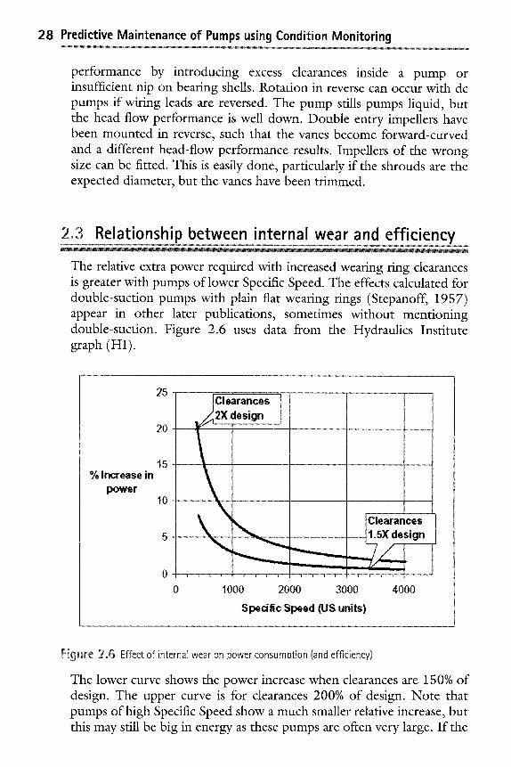
The relative extra power required with increased wearing ring clearances is greater with pumps of lower Specific Speed. The effects calculated for double-suction pumps with plain flat wearing tings (Stepanoff, 1957) appear in other later publications, sometimes without mentioning double-suction. Figure 2.6 uses data from the Hydraulics Institute graph (HI).
% Increase in power
20-
15-
1 0 "~
. . . . . . . . . . . . . . . . . . .
~
Clearances 2X design
Clearances 1.5X design
1000 2000 3000 4000
Spedfic Speed (US units)
Figure 2.,6 Effect of internal wear on power consumption (and efficiency)
The lower curve shows the power increase when clearances are 150% of design. The upper curve is for clearances 200% of design. Note that pumps of high Specific Speed show a much smaller relative increase, but this may still be big in energy as these pumps are often very large. If the
2 �9 Pump performance and the effect of wear 29
clearances, the Specific Speed, and the power cost for the pump in question are known, the increase in power consumption and then annual operating cost can be estimated using these curves (Bloch and Geimer, 1985). Unless the engineer has a good correlation between the state of clearances and detected performance degradation, this method can only be used if the pump is dismantled.
With multi-stage pumps, the sealing tings provide an additional bearing effect for their longer shafts. When the clearances increase significantly, vibration can increase. Vibration monitoring is also used to detect other problems which occur with most rotating machines, such as unbalance, misalignment, looseness, bearing wear. Monitoring of overall vibration levels at the bearings and of selected frequencies or frequency bands is recommended as for most rotating machinery. (See Chapters 6 and 7).
2.,4 Rate of wear
Wear in a pump is primarily velocity dependent, and wear rate is typically proportional to local velocities to the power of two or more. The head requirement dictates the wear in the casing as it relates directly to the tip velocity of the impeller (Astall, 2000).
The wear rate of a pump also varies with the liquid pumped and materials of construction. In slurry duty, life may be only a few hundred hours. For example, in one water supply utility with long experience of condition monitoring of pumps, rates noted are: stainless steel/ stainless, 1% per year; CI /bronze, 2.4%, CI/gunmetal , 2%.
An average deterioration in efficiency from supplied condition of 8% over 10 years was found in the water industry from testing over 300 medium to large split casing pumps. The pumps had the usual cast iron casings and bronze or gunmetal impellers, and leaded bronze wearing rings and bushes (Fleming, 1992). Deterioration remained fairly constant at about 9% with age between 12 and 24 years then decreased again to 16% at 40 years. The deterioration is considered to be mainly due to surface finish corrosion and buildup of corrosion products in casings. Analysis of one installation of 6 pumps over 15 years also showed the value of refurbishment, given that the cost of operation is much greater than initial cost.
Plants often have spared pumps that can remain on standby for long periods, yet are intended to start up instantly and take over duty reliably. Seal deterioration, contaminant ingress, and brinelling of bearings from transmitted vibration have all occurred. Standby pumps
30 Predictive Maintenance of Pumps using Condition Monitoring
should be run regularly for at least one hour about every four to six weeks (Bloch, 1997).
Karassik considers that boiler feed pumps made of stainless steel should last 50 000h to 100 000h between overhauls. API 610 (API, 1995) expects 20 000h in continuous operation.
Operation away from BEP shortens pump life. This is more pronounced in large pumps. Table 2.2 gives the view of Bloch and Geitner (1985) on the effect of a varying load profile, and somewhat similar information is given by Karrassik for pumps of different types and sizes.
Table 2~2 Influence on pump life of operating away from BEP
% maximum life
if run ot 50% BEP
% maximum life
if run ot 30% BEP
% maximum life
if run ot 20% BEP
Small pump (<30kW) 95010 90Olo 80Olo Mid-size pump (<450kW) 90Olo 70Olo 60Olo Multistage pump (<3000kW) 75% 50% 30% Large multistage pumps (< 18 500kW) 600/0 25% 0
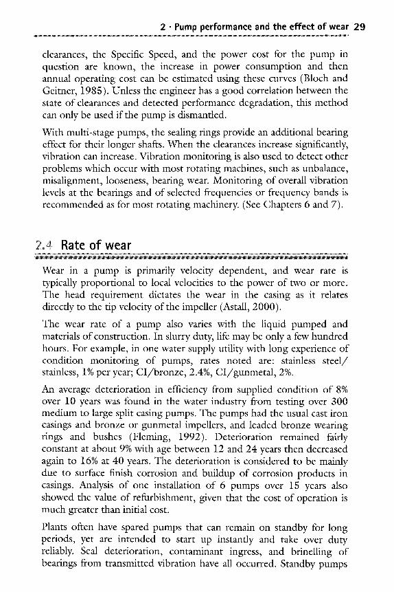
Data from regular condition monitoring tests of a 230kW pump on cooling water (design duty 4 5 0 L / s @ 41m) is shown in Figures 2.7 and 2.8. The Percentage Reduction in Performance is calculated for the head values at a datum flow, usually the design flow. If test points are below the datum flow, the shape of the curve is extrapolated across to the flow. One point was inconsistent (700 hours) and therefore is not included (pumps do not repair themselves). The correlation to linear is R2=0.9884.
18
1 6 -
I ! /~ - - z
z 12 _o I - -
1 0 - 2~
, ~ 8 - -
< 6 - -
Z
0 .....
0
!
. . . . . . . . . . . . . . L . . . . . . {..
" i
I . i
]" r ..................... 500 1000 1500
DAYS IN SERVICE
Figure 2.7 Degradation of a pump with time (trendline)
2 �9 Pump performance and the effect of wear 31
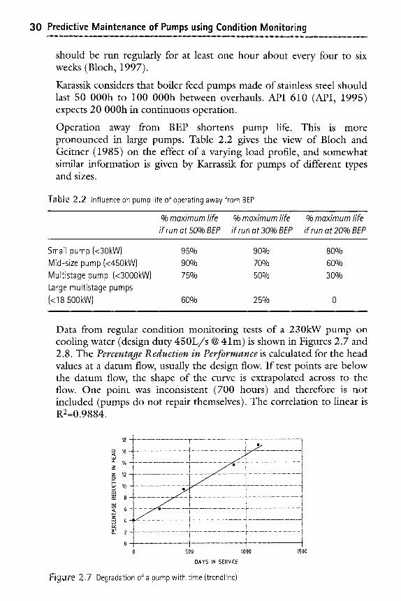
Figure 2.8 shows all the data points as recorded in the plant, where vibration trending software was adapted to performance analysis. The warning levels selected are shown.
~
-2
-4
-6
" - - 8 . c - . m
LLI -10_
2 2 )
i ,_J ~_ -I0_
O/o AUX COOLING PUMP 1
PERCENTAGE DOWN IN PERFORMANCE
0~i r z o?, - ? " ' r~.
0 . . . 0 , , ,
�9 .Q t-v- ,-- �9 .. ~_
"".... i "-.. (3")
....... 0 ......... Q. """"....... ........................... "':...... o')~176
i ...... �9 . . . . . . . . . . . . . "- Z
'-. ZD -
-15
-18_
-20
-22
O ~ - o?, r v -
J~
.... "' '""'""""qL
ALERT
:'-'--.........~"
0.. -..... "-...
..... . .....
FAULT
I I I I I I I I I I
0 200 400 600 800 1000 1200 Days: 11-JAN-96 TO 05-MAR-89
Figure 2~ Degradation of a pump with time (actual results)
2~ Pump selection reliability factors
At the pump selection stage, a Reliability Index can be helpful in assessing reliability of a given design (Bloch and Geitner, 1994). Three major influences are considered to affect reliability: operating speed, impeller diameter and flow rate. The Reliability Index is given from the product of the factors assigned to each, and will range between zero and unity.
The rate of wear in rubbing surfaces is considered to be linear with speed, so the Speed factor varies from 0.2 for the maximum design speed to 0.6 at half that speed. An Impeller Diameter factor allows for changes away from the optimum diameter for a casing, and is also affected by speed. A Flow Rate factor allows for variations in flow from best efficiency point, and also varies with pump size. Energy and Cost
32 Predictive Maintenance of Pumps using Condition Monitoring
factors are also included in pointing to the final selection. Full details and charts are given in the reference. The approach could also be helpful is assessing reliability performance of an existing pump.
2oG Case studies in detected performance shortfall
Sometimes there are other problems where poor pump performance is detected that do not fit into the above categories.
2.6.1 Pump running backwards
A large electric generator with water-cooled stator windings commonly has three stator cooling pumps: two ac motor driven 100% duty, with one normally on standby, and a emergency dc motor driven pump. Automatic switching is based on measured flow, or simply with a flap type flow detector.
Reported suspect performance on the dc pump led to a field test. An orifice plate was designed and installed in a suitable flanged joint. Performance of the pump was verified as low, but the tester noticed that the pump was rotating in the reverse direction. During reinstallation after some work, the wires had apparently been reversed. Pumps running backwards will still pump, but not at the desired rate. There was little of the drive shaft readily visible to observe rotation.
2.6.2 Drive coupling bolts sheared
Boiler feed pumps of recent design operating at speeds above 3000 r / m i n usually have a suction booster pump in series with the main pump, designed to cope with low NPSH (ie Net Positive Suction Head). A usual arrangement is to have the booster pump driven direct from the motor, and the main pump driven through a step-up gearbox at higher speed. One such an installation, it was noticed that the motor current was much less on one pump of an "identical" pair. Pieces of bolt type material underneath the booster pump drive coupling led to an examination with a stroboscope. The drive coupling bolts had all sheared off. Although the booster pump was not being driven, it was rotating because of the flow drawn through it by the main pump. Fortunately, the main pump incurred no damage during this time while it was not receiving the desired higher suction pressure.
2 �9 Pump performance and the effect of wear 33
2.6.3 Impeller smaller than expected A pair of ash slurry disposal pumps were installed in each of four stages of a coal fired power station. The disposal point was some kilometres away at one end of the plant. This had been considered in the design, and although the four sets of pumps had identical casings, progressively smaller impellers and motors were supplied at each stage to suit the shorter duty distance.
The first pump to be overhauled had been returned from the repair workshops and installed. Unexpectedly, it could not handle the usual duty flow and adverse comments were made about the quality of the overhaul. The workshops proved that a new impeller had been installed, and all clearances and settings were on specification. Condition monitoring established that performance was indeed below par, and deduced that a smaller impeller than the original had been fitted. Inspection through a casing port verified this. The repair workshops did not know of the different impeller sizes, and had obtained a spare impeller from store that was not specifically marked for location.
References
Addie, G; Pagalthivarthi, KV and Visintainer, R (1996) Slurry pump wear factors Pumps and Systems October [Article]
API 610 Centrifugal pumps for refinery, heavy duty chemical and gas industry service 8th edition, American Petroleum Institute, Washington 1995 (9th Edition titled Centrifugal pumps for petroleum, petrochemical and natural gas industries due 2003) [Standard]
Astall, R (2000) Are your centrifugal pumps running too slowly? Engineers Australia, March [Article]
Bachus, L and Custodio, A (2003) Know and understand centrifugal pumps Elsevier, UK [Book]
Bloch, HP and Geitner, FK (1985) Practical machinery management for process plants Vol 4 Major process equipment maintenance and repair Gulf, Houston [Book]
Bloch, HP and Geitner, FK (1994) Introduction to machine reliability and assessment Gulf, Houston 2nd Edition [Book]
Bloch, HP (1997) Why you should run spare pumps Hydrocarbon Processing July, Vol 76, No 7 [Article]
Fabeck, PH and Erickson, RB (1990) IS05199 standard addresses today's reliability requirements for chemical process pumps Proceedings of 7th International Pump Users Symposium, Texas A&M University [Paper]

34 Predictive Maintenance of Pumps using Condition Monitoring
Fleming, JM (1992) The new concept of effectiveness of through life pump cost management Fluid machinery ownership costs MEP, [Book]
HI (1994) Efficiency prediction method for centrifugal pumps, in Energy reduction in pumps and pumping systems, Hydraulics Institute, [Video course]
HI, www.pumps.org PDF diagrams: Fig 1.78A (Hydraulics Institute, USA) [Website]
Karassik, IJ and Grieve, T (1998) Centrifugal pumpsChapman & Hall [Book]
Karassik, IJ (1988) Centrifugal Pump Clinic 2nd Ed Marcel Dekker [Book]
KSB (1990) Centrifugal pump lexicon 3rd Ed KSB, Frankenthal [Book]
Ludwig, G; Meschkat, S; Stoffel, B (2003) Design factors affecting pump efficiency Energy Efficiency in Motor Driven Systems, Eds Parasiliti, F and Bertoldi, P, Springer, Berlin [Book}
SIHI (1988) Basic principles for the design of centrifugal pump installations SIHI-Halberg [Book]
Stepanoff, AJ (1957) Centrifugal and axialflow pumps Wiley [Book]
Turton, RK (1994) Rotodynamic Pump Design Cambridge University Press, [Book]
13 Performance analysis and testing of pumps for condition monitoring i Performance analysis needs performance data m Temperature m Pressure
Flow Z Speed ,E Power m Efficiency calculation i Pumps in systems and relationship to CM
3~ Performance analysis needs performance data
Performance analysis requires repeatable measurements of process parameters such as temperature, pressure, flow, displacement, speed, power and time. Of all the techniques available for condition monitoring, it is the least widely discussed.
Experience will show whether sufficient repeatability is obtained by use of permanent instrumentation. Readings can be made manually and processed manually or by computer. Improved productivity and accuracy result from use of a hand-held data collector for subsequent downloading into a computer for processing. Permanent plant computer systems may be able to be set up and used to calculate and display condition-monitoring parameters - once repeatability and readability of the available indications has been assured.
Recent developments look promising in transducers used for permanent installation (Eryurek and Warrior, 1997, Frerichs, 1999 and Szanyi et al, 2003) and in on-line calibration (Hines et al, 2001). Systems are now available that can be programmed to continually monitor DCS data and highlight changes in variables or in parameters calculated from

36 Predictive Maintenance of Pumps using Condition Monitoring
them, and send web-based reports (e.g. SmartSignal's eCM). Golden Eye, part of Honeywell's Asset@MAX, allows staff to read real-time process information on a handheld unit while in the plant, and to also enter field data. Specifically for pumps, the Tech-Sys Corp DolphinPLUS provides extensive control and monitoring. Thermometric systems are also available for permanent monitoring (see Section 5.5) As these systems advance in capability, details in any book would soon be out of date, and it is recommended to maintain awareness from websites.
Even if the stringent conditions required by Standards such as those for flow measurement (ISO 5167:1996) do not exist, useful data suitable for condition monitoring can be gained by adapting these methods. Some brief points follow.
Pumps with impeller blade adjustment (i.e. variable pitch blades), or with prerotation control by variable pitch non-rotating inlet vanes have a family of performance curves, and will therefore need to be tested at standardised settings for comparisons.
Performance analysis is also applicable for other plant items that may be associated with pumps, such as heat exchangers, steam turbines and mechanical controls linkages (Beebe, 1994, 2000a, 2000b, 2001, 2003).
3~ Temperature
Calibration of primary elements does require special facilities, such as stirred liquid salt bath furnaces, or dry-well types. Thermocouples of the steel-sheathed mineral insulated type are reliable, if calibrated, and their use with digital temperature indicators is convenient.
Where thermowells (i.e. thermo pockets) are available in pipe walls, resistance elements (i.e. RTD) give the highest accuracy up to about 600~ and are more stable than thermocouples. For lower temp- eratures, calibrated mercury-in-glass thermometers are often a simple method.
Provided the conditions are repeatable (i.e. not in a high breeze), measurement on the pipe surface can often be a sufficient indicator of the liquid temperature and can be read with contact or non-contact thermometers.

3 �9 Performance analysis and testing of pumps for condition monitoring 37
3~ Pressure
Total Head is the total energy added by the pump to the liquid, and is measured in the field using pressures read at pump suction and discharge flanges, where threaded tapping holes are usually provided, and are plugged if no permanent instrument is installed.
Head is referred to the pump centreline. If the suction and discharge tappings and instruments are not at the same level (based on centre of the scale for gauges), allowance must be made for liquid heads in the tapping lines. If the instrument is below the tapping, then it will read too high, and the static liquid leg must be measured and subtracted from the reading, and vice versa. This static leg effect becomes smaller in proportion with higher line pressures, and will be negligible at high pressures. The relationship is, with pressure P in Pa, density p in k g / m 3, is:
P - p g H
and the equivalent Head in metres of liquid is = Pr essure(kPa) • 1000
Density (kg/m 3 ) • g
For fresh water at temperatures near ambient, l m -- 9.8 lkPa is suitable for most practical purposes. For seawater, l m = 10.1kPa. For other temperatures and pressures, or for other liquids, tables of properties should be consulted (e.g. via www.pepse.com for water). Where the density of the liquid varies or is not known, as with ash slurry, a sample may be required to find the density.
In other commonly used units, lkPa = 6.895 psi. The equivalent pressure to a reading on a mercury manometer varies with density according to the above formula. At 0~ l m m H g = 0.1333kPa, 1 inHg = 3.386kPa. At 20~ l m m H g = 0.1329kPa, 1 inHg = 3.375kPa. Mercury has become less used on occupational health and safe~, grounds.
For testing pumps, as we are interested in the difference in pressure~; across the pump, gauge pressures are sufficient. If desired, the absolute pressure can be obtained by adding the atmospheric pressure to gauge pressure values. The normal atmospheric pressure of 101.3 kPa = 14.7 psia = 30 inches Hg.
As the suction pressure may be negative, care is needed with the arithmetic to obtain the total head from the generated pressure.
38 Predictive Maintenance of Pumps using Condition Monitoring
3.3.1 Instruments for pressure
If the instruments are positioned at the same cent_reline elevation, then the generated pressure will be given by the difference in the readings, allowing for calibration and if the suction pressure is negative (i.e. below atmospheric).
Pump suction pressures are often below atmospheric. This can cause the piping connecting the instrument to become filled with vapour (water vapour and air which un-dissolves from the liquid) rather than liquid. The static leg of vapour is negligible. If in doubt, use clear plastic piping, or position the instrument at pump cent_reline. Tapping lines should be bled to ensure they are filled with liquid or vapour, as the case may be. To check contents of instrument line and transducer sensitivity, lower the transducer a metre and check that the reading changes by this amount.
Bourdon test quality pressure gauges, calibrated at around the range of use, are satisfactory and can be expected to give accuracy of +0.25% or better if treated carefully. Industrial quality types can be acceptable if carefully calibrated and cared for. Many types of electronic transducer are available, and are necessary if a computer-based data collection and
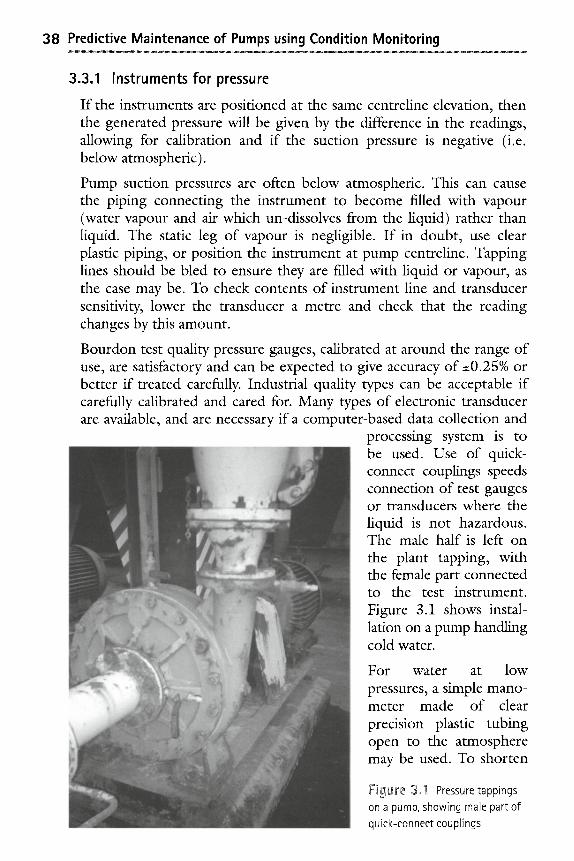
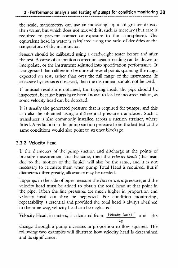
processing system is to be used. Use of quick- connect couplings speeds connection of test gauges or transducers where the liquid is not hazardous. The male half is left on the plant tapping, with the female part connected to the test instrument. Figure 3.1 shows instal- lation on a pump handling cold water.
For water at low pressures, a simple mano- meter made of clear precision plastic tubing open to the atmosphere may be used. To shorten
Figu~-'e 3ol Pressure tappings on a pump, showing male part of quick-connect couplings
3 �9 Performance analysis and testing of pumps for condition monitoring 39
the scale, manometers can use an indicating liquid of greater density than water, but which does not mix with it, such as mercury (but care is required to prevent contact or exposure to the atmosphere). The equivalent head in water is calculated using the ratio of densities at the temperature of the manometer.
Sensors should be calibrated using a deadweight tester before and after the test. A curve of calibration correction against reading can be drawn to interpolate, or the instrument adjusted into specification performance. It is suggested that calibration be done at several points spanning the range expected on test, rather than over the flail range of the instrument. If excessive hysteresis is observed, then the instrument should not be used.
If unusual results are obtained, the tapping inside the pipe should be inspected, because burrs have been known to lead to incorrect values, as some velocity head can be detected.
It is usually the generated pressure that is required for pumps, and this can also be obtained using a differential pressure transducer. Such a transducer is also commonly installed across a suction strainer, where fitted. A reduction in the pump suction pressure from the last test at the same conditions would also point to strainer blockage.
3.3.2 Velocity Head
If the diameters of the pump suction and discharge at the points of pressure measurement are the same, then the velocity heads (the head due to the motion of the liquid) will also be the same, and it is not necessary to calculate them when pump Total Head is required. But if diameters differ greatly, allowance may be needed.
Tappings in the side of pipes measure the line or static pressure, and the velocity head must be added to obtain the total head at that point in the pipe. Often the line pressures are much higher in proportion and velocity head can then be neglected. For condition monitoring, repeatability is essential and provided the total head is always obtained in the same way, velocity head can be neglected.
Velocity Head, in metres, is calculated from: [Velocity (re~s)] 2 and the 2g
change through a pump increases in proportion to flow squared. The following two examples will illustrate how velocity head is determined and its significance.
40 Predictive Maintenance of Pumps using Condition Monitoring
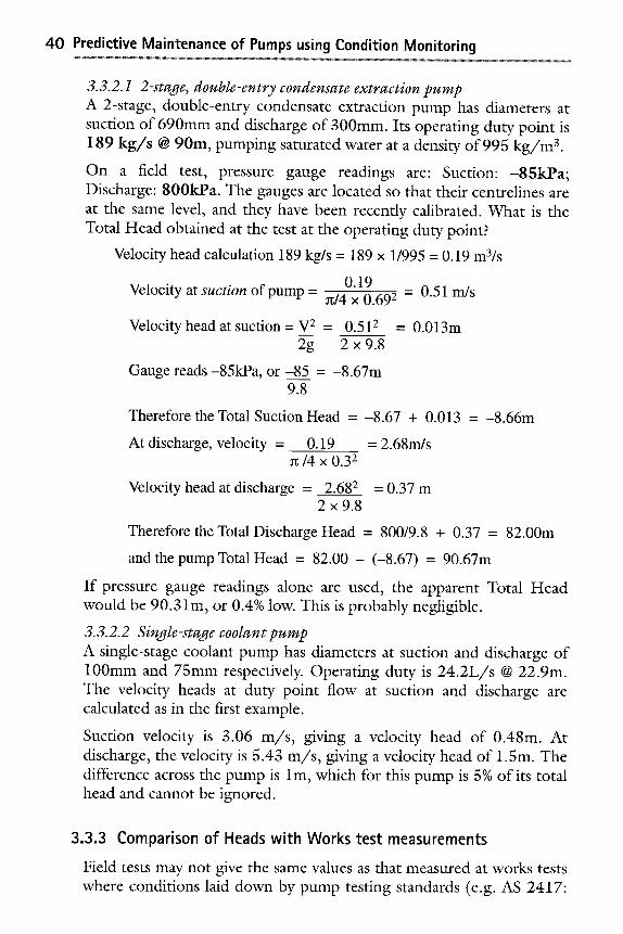
3.3.2.1 2-stage, double-entry condensate extraction pump A 2-stage, double-entry condensate extraction pump has diameters at suction of 690mm and discharge of 300mm. Its operating duty point is 189 k g / s @ 90m, pumping saturated water at a density of 995 k g / m 3.
On a field test, pressure gauge readings are: S u c t i o n : - 8 5 k P a ; Discharge: 800kPa. The gauges are located so that their centrelines are at the same level, and they have been recently calibrated. What is the Total Head obtained at the test at the operating duty point?
Velocity head calculation 189 kg/s = 189 x 1/995 = 0.19 m3/s
0.19 Velocity at suction of p u m p - n/4 x 0.692 = 0.51 m/s
Velocity head at suction = V 2 = 0.512 = 0.013m 2g 2 x 9.8
Gauge reads-85kPa, or -85 = -8.67m 9.8
Therefore the Total Suction Head = -8.67 + 0.013 = -8.66m
At discharge, velocity = 0.19 = 2.68m/s ~t/4 x 0.32
Velocity head at discharge = 2.682 = 0.37 m 2 x 9 . 8
Therefore the Total Discharge Head = 800/9.8 + 0.37 = 82.00m
and the pump Total Head = 82.00 - (-8.67) = 90.67m
If pressure gauge readings alone are used, the apparent Total Head would be 90.3 lm, or 0.4% low. This is probably negligible.
3.3.2.2 Single-stage coolant pump A single-stage coolant pump has diameters at suction and discharge of 100mm and 75mm respectively. Operating duty is 24 .2L / s @ 22.9m. The velocity heads at duty point flow at suction and discharge are calculated as in the first example.
Suction velocity is 3.06 m / s , giving a velocity head of 0.48m. At discharge, the velocity is 5.43 m / s , giving a velocity head of 1.5m. The difference across the pump is lm, which for this pump is 5% of its total head and cannot be ignored.
3.3.3 Comparison of Heads with Works test measurements
Field tests may not give the same values as that measured at works tests where conditions laid down by pump testing standards (e.g. AS 2417"
3 �9 Performance analysis and testing of pumps for condition monitoring 41
1993, or BS ISO EN 5198:1999) are followed with pressure measure- ments are made two pipe diameters away from the pump flanges (to avoid any recirculation effects). Four tappings around the pipe are used, each with its own isolating valve, and connected by a piezometric ring. If individual measurements from each tapping show no difference, a single instrument may be connected to the ring and used. Such tappings are rarely provided in the field.
The effect of these differences can be significant, and in critical cases such as when disputing guarantee performance, the special tappings would need to be installed. As an example of comparison on a 22 m3/h pump where both types of pressure tappings were used, at best efficiency point the head was 10% higher and efficiency 5% higher using tappings at the pump flanges (Yedidiah, 1996).
For investigating the matching of a pump to a system, any such effects would affect both pump performance and system equally, and this refinement can be ignored. For condition monitoring, this effect would be constant with time, and can also be ignored.
3~ Flow
Complex pumps may have separate sealing flows into and/or from their shaft glands that bypass the pump flow measuring point. Usually these are very small in comparison and variations from design may be neglected for condition monitoring. For critical pumps, separate gland sealing flow metering may be justified, particularly if the glands can be repaired without dismantling the complete pump. Measurement of sealing water flow can be useful for slurry pumps.
For pumps in parallel, if each pump can be tested in turn, flow measurement at a single location in the combined inlet or outlet piping will save setup time and cost.
Each case must be examined to ensure that any minimum flow leakoff valve leakage or axial thrust balance device flows are properly allowed for to ensure that flow through the pump is obtained. Methods of flow measurement using differential pressure devices lose usefulness at low flows where the differential pressure is very small.
3.4.1 Orifice plates
Orifice plates can be made cheaply and one may be able to be inserted at an existing flanged joint in piping. The equations used in Standards
42 Predictive Maintenance of Pumps using Condition Monitoring
such as ISO5167-1.1997 are used. The simplest arrangement for pressure tappings is to locate them at distances from the orifice plate of one pipe diameter upstream, half a diameter downstream (called D and D/2 ) . Repeatable results suitable for condition monitoring are possible with much shorter lengths of straight piping upstream and downstream than required by such standards. For many years, satisfactory results have been gained with a series of 24 boiler feed pumps where the upstream straight length is only one diameter.
High energy pumps usually have a flow metering orifice plate or other device to initiate low flow protection. Such orifice plates have been found to hold their edge condition for many years on boiler feedwater duty. Care must be taken when connecting and bleeding a test transducer, so that a sudden low differential pressure is not sensed by the service instrument, or otherwise the protection will be initiated!
In some pumps, the balance device leakoff flow is returned upstream of the flow measuring device in the pump suction line. This means that the balance water flow is included in the total flow through the pump, and the device will indicate higher than the pump duty flow. This arrangement is not in accord with good industry practice as it will affect the pump automatic minimum flow protection opening and closing points. As the pump output flow is required for condition monitoring, on such pumps, the balance flow must be measured as well as the main flOW.
From IS05167-1.1997, the general equation for flow is:
qm - CEe ~ d 242App~ 4
with symbols defined in Table 3.1
Charts in the Standard give data on the effects of Reynolds Number, which is a non-dimensional parameter calculated from diameter, kinematic viscosity, density and velocity.
3.4.2 Withdrawable double-tip pitot tube devices
Withdrawable double-tip pitot tube devices are available (or can be made: Beebe, 2001) and installed in pipes under moderate pressures. These are installed when required through a suitable gland fitting, in a gate valve screwed into a socket welded on the pipe wall. If the flow is not expected to change significantly, a traverse across the pipe at the Standard positions (Beebe, 2001) can relate the centre velocity to the average. Future tests can then be made with centre measurements only using these single-point probes. The upstream and downstream sensing
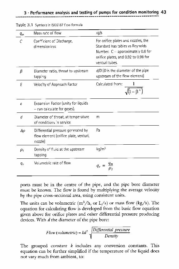
3 �9 Performance analysis and testing of pumps for condition monitoring 43
Table 3.1 Symbols in IS05167 flow formula
qm Mass rate of flow kg/s
C Coefficient of Discharge, dimensionless
For orifice plates and nozzles, the Standard has tables vs Reynolds Number. C = approximately 0.6 for orifice plates, and 0.92 to 0.98 for venturi tubes.
/3 Diameter ratio, throat to upstream tapping
d/D(D is the diameter of the pipe upstream of the flow element)
Velocity of Approach Factor Calculated from: ]
40--134 ) Expansion Factor (unity for liquids - can calculate for gases).
d Diameter of throat, at temperature m of conditions in service
Ap Differential pressure generated by Pa flow element (orifice plate, venturi, nozzle)
,01 Density of fluid at the upstream kg/m 3 tapping
qv Volumetric rate of flow qm
Pl
ports must be in the centre of the pipe, and the pipe bore diameter must be known. The flow is found by multiplying the average velocity by the pipe cross-sectional area, using consistent units.
The units can be volumetric (m3/h, or L/s) or mass flow (kg/s). The equation for calculating flow is developed from the basic flow equation given above for orifice plates and other differential pressure producing devices. With d the diameter of the pipe bore:
Flow (volumetric) - kd 2 ]Differential pressure Density
The grouped constant k includes any conversion constants. This equation can be further simplified if the temperature of the liquid does not vary much from ambient, to :
44 Predictive Maintenance of Pumps using Condition Monitoring
Flow (volumetric) - k 2 ~/Differential pressure
However, this last simplification should be used with due care. An example of incorrect use was the acceptance test of a steam turbine generator that relied on feedwater flow measurement using a venturi. This had been calibrated at the maker's works at 20~ using a flow tank, and the simplified characteristic formula provided. However, the water temperature at site was 150~ The effect of not making the correct allowance for the diameter of the venturi bore enlarging at site conditions was >> 0.5% error - quite significant when large sums of money are involved if the guaranteed performance is not met.
3.4.3 Ultrasonic flowmeters
Ultrasonic flowmcters measure and display the mean velocity of flow without access to the pipe contents. Although accuracy is not always high, good repeatability is obtained, and these have been widely used with success for pump condition monitoring. Types using two different principles are available, and it is recommended that such devices be tried in the proposed application before purchase. Sensors should be mounted on the side of the pipe, in as long a straight length as can be found.
Setting up time is only a few minutes, and they work with most liquids. Some types only show instantaneous flow rate, but those that also integrate flow over time are preferable, as fluctuations in flow are smoothed out. Types are available for use on pipes coveting a range between 13mm and 5m diameter, with a turndown ratio of 500 to 1. Accuracy of 0.5% to 2% of reading is claimed, and can take pipe surface temperatures of up to 260~
The pipe bore diameter must be known. If this is likely to change over time from bore deposits, then a spool piece that can be removed for cleaning is recommended. Another possibility is to make it from non- corrosive material. Cement and other linings may cause difficulties.
3.4.3.1 The transit-time method The transit-time method uses two sensors, which are clamped on opposite sides of the pipe, or at a set distance apart. Ultrasonic pulses are alternatively transmitted through the liquid in one direction, and then in the opposite direction. Liquid velocity is found from the measured time difference between the pulse arrival at the receiver. Accuracy of +1% may be expected. The method does not work in all cases, as suspended solids or fine bubbles cause the ultrasonic pulse to be scattered.
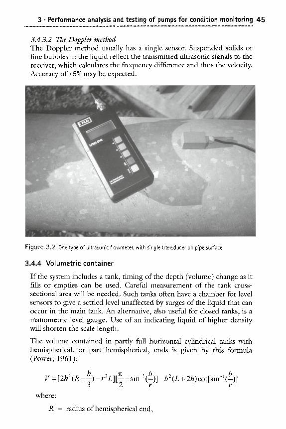
3 �9 Performance analysis and testing of pumps for condition monitoring 45
3.4.3.2 The Doppler method The Doppler method usually has a single sensor. Suspended solids or fine bubbles in the liquid reflect the transmitted ultrasonic signals to the receiver, which calculates the frequency difference and thus the velocity. Accuracy of +5% may be expected.
Figure 3.2 One type of ultrasonic flowmeter, with single transducer on pipe surface
3.4.4 Volumetric container
If the system includes a tank, timing of the depth (volume) change as it fills or empties can be used. Careful measurement of the tank cross- sectional area will be needed. Such tanks often have a chamber for level sensors to give a settled level unaffected by surges of the liquid that can occur in the main tank. An alternative, also useful for closed tanks, is a manometric level gauge. Use of an indicating liquid of higher density will shorten the scale length.
The volume contained in partly full horizontal cylindrical tanks with hemispherical, or part hemispherical, ends is given by this formula (Power, 1961):
h 7~ V-[2hZ(R--~)+rZL][} sin-~ ( b ) ] - b r
where:
2(L + 2h)cot[sin -~ (b)] r
R = radius of hemispherical end,
46 Predictive Maintenance of Pumps using Condition Monitoring
h = height of hemispherical end from crown (= R when end is a full half-sphere),
r = radius of tank inside, b = distance from centreline of liquid level,. L = length of parallel part of tank.
If the liquid level is below the centerline, V gives the volume of liquid contained. If the liquid level is above the centreline, V--volume of empty space above the liquid.
For small flows, such as the crankcase return oil flow on hydraulic pumps, a smaller container such as laboratory glassware is used.
3.4.5 Other methods
Other methods may be applicable, and brief details are given for information.
3.4.5.1 Dye dilution Dye dilution has been used on power station cooling water pumps to measures flow typically within 1%. Fluorescent dye is injected at a known closely controlled rate into the suction or discharge of the pump being tested. Further done the system when thorough mixing has occurred, samples are drawn over about 20 minutes, and the concen- tration read using a fluorometer. A dye calibration curve is obtained with a water sample and different concentrations of die added. Only one pump can be run and tested at a time on multi-pump systems.
3.4.5.2 Measurement of the co-ordinates Measurement of the co-ordinates of free discharge outflow from a pipe is a rough method where approximate flows are required. Equations are available for pipes discharging at angles from vertical to downwards angles from horizontal (Beebe, 2001).
3.5 Speed Speed changes affect head, flow and power. According to the pump affinity law relationships, Flow varies directly with speed, Head varies with speed squared, and Power with speed cubed. For variable speed pumps, speed must therefore be measured and corrections made to datum values of parameters for trending, as shown in Section 4.1.4.
The speed of induction motors varies directly in proportion to any changes in supply system frequency, and is also affected slightly by changes in supply voltage. For example, on a 50Hz supply system, a
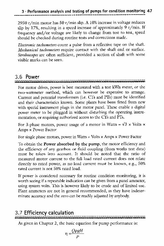
3 �9 Performance analysis and testing of pumps for condition monitoring 47
2950 r /min motor has 50 r /min slip. A 10% increase in voltage reduces slip by 17%, resulting in a speed increase of approximately 9 r /min. If frequency and /o r voltage are likely to change from test to test, speed should be checked during routine tests and corrections made.
Electronic tachometers count a pulse from a reflective tape on the shaft. Mechanical tachometers require contact with the shaft end or surface. Stroboscopes are often sufficient, provided a section of shaft with some visible marks can be seen.
3.6 Power
For motor drives, power is best measured with a test kWh meter, or the two-wattmeter method, which can however be expensive to arrange. Current and potential transformers (i.e. CTs and PTs) must be identified and their characteristics known. Some plants have been fitted from new with special instrument plugs in the motor panel. These enable a digital power meter to be plugged in without disturbing the operating instru- mentation, or requiring authorized access to the CTs and PTs.
For 3-phase motors, power usage of a motor in Watts -- ~/3 x Volts x Amps x Power Factor
For single phase motors, power in Watts -- Volts x Amps x Power Factor
To obtain the Power absorbed by the pump, the motor efficiency and the efficiency of any gearbox or fluid coupling (from works test data) must be taken into account. It should be noted that the ratio of measured motor current to the full load rated current does not relate directly to rated power, as no-load current must be known, e.g., 50% rated current is not 50% rated load.
If power is considered necessary for routine condition monitoring, it is worth seeing if a repeatable indication can be given from a panel ammeter, using system volts. This is however likely to be crude and of limited use. Plant ammeters are not in general recommended, as they have indeter- minate accuracy and the zero can be readily adjusted by anybody.
3.7 Efficiency calculation
As given in Chapter 2, the basic equation for pump performance is"
QpgH P
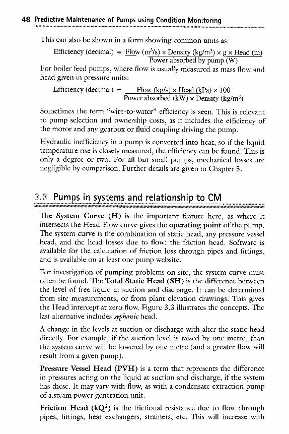
48 Predictive Maintenance of Pumps using Condition Monitoring
This can also be shown in a form showing common units as:
Efficiency (decimal) - Flow (m3/s) x Density (kg/m 3) x g x Head (m) Power absorbed by pump (W)
For boiler feed pumps, where flow is usually measured as mass flow and head given in pressure units:
Efficiency (decimal) - Flow (kg/s) x Head (kPa) x 100 Power absorbed (kW) x Density (kg/m 3)
Sometimes the term "wire-to-water" efficiency is seen. This is relevant to pump selection and ownership costs, as it includes the efficiency of the motor and any gearbox or fluid coupling driving the pump.
Hydraulic inefficiency in a pump is converted into heat, so if the liquid temperature rise is closely measured, the efficiency can be found. This is only a degree or two. For all but small pumps, mechanical losses are negligible by comparison. Further details are given in Chapter 5.
3~ Pumps in systems and relationship to CM ~ m ~ ~ m l m l m m l m m L ~
The System Curve (H) is the important feature here, as where it intersects the Head-Flow curve gives the operating point of the pump. The system curve is the combination of static head, any pressure vessel head, and the head losses due to flow: the friction head. Software is available for the calculation of friction loss through pipes and fittings, and is available on at least one pump website.
For investigation of pumping problems on site, the system curve must often be found. The Total Static H e a d (SH) is the difference between the level of free liquid at suction and discharge. It can be determined from site measurements, or from plant elevation drawings. This gives the Head intercept at zero flow. Figure 3.3 illustrates the concepts. The last alternative includes syphonic head.
A change in the levels at suction or discharge with alter the static head directly. For example, if the suction level is raised by one metre, than the system curve will be lowered by one metre (and a greater flow will result from a given pump).
Pressure Vessel Head ( P V H ) is a term that represents the difference in pressures acting on the liquid at suction and discharge, if the system has these. It may vary with flow, as with a condensate extraction pump of a.steam power generation unit.
Frict ion Head (kQ 2) is the frictional resistance due to flow through pipes, fittings, heat exchangers, strainers, etc. This will increase with
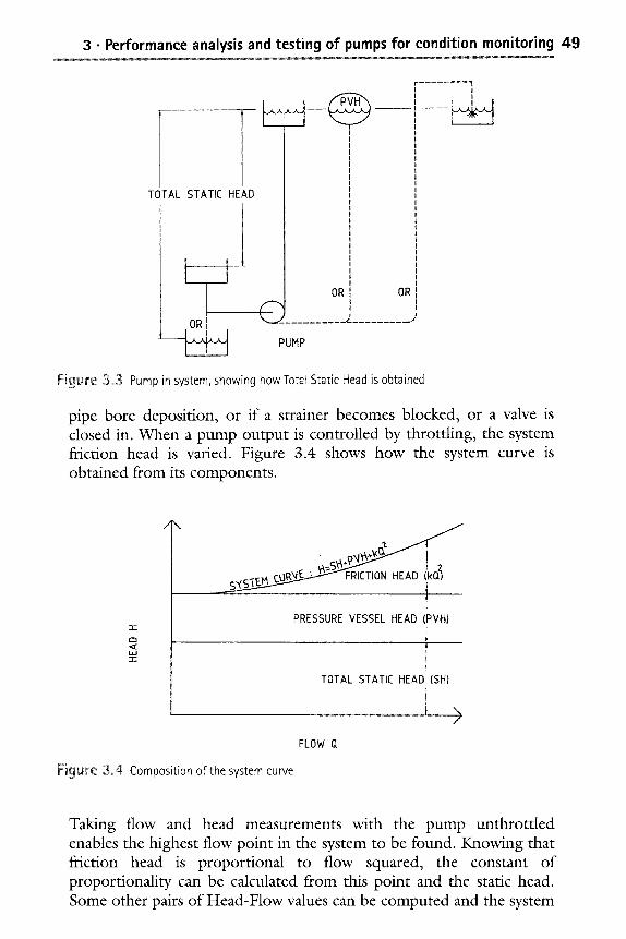
3 �9 Performance analysis and testing of pumps for condition monitoring 49
TOTAL STATIC HEAD
I ....... I 1 ORI ~-"
' ~ ' ~ PUMP
I I I
I I
I I I I I ! I
1 t
I !
I I
OR I ! ! 1
OR i
. /
Figure 3.3 Pump in system, showing how Total Static Head is obtained
pipe bore deposition, or if a strainer becomes blocked, or a valve is closed in. When a pump output is controlled by throttling, the system friction head is varied. Figure 3.4 shows how the system curve is obtained from its components.
. . . . . . . . . . . . . . . . . . i . . . . . PRESSURE VESSEL HEAD (PVH)
TOTAL STATIC HEAD (SH) !
i
/
FLOW Q
Figure 3~ Composition of the system curve
Taking flow and head measurements with the pump unthrottled enables the highest flow point in the system to be found. Knowing that friction head is proportional to flow squared, the constant of proportionality can be calculated from this point and the static head. Some other pairs of Head-Flow values can be computed and the system
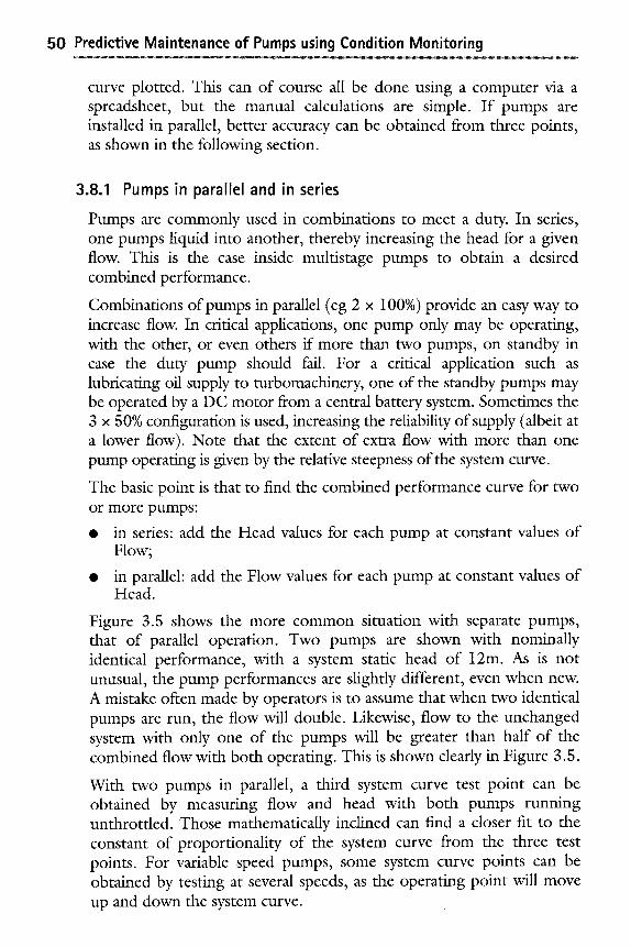
50 Predictive Maintenance of Pumps using Condition Monitoring
curve plotted. This can of course all be done using a computer via a spreadsheet, but the manual calculations are simple. If pumps are installed in parallel, better accuracy can be obtained from three points, as shown in the following section.
3,8,1 Pumps in parallel and in series
Pumps arc commonly used in combinations to meet a duty. In series, one pumps liquid into another, thereby increasing the head for a given flow. This is the case inside multistage pumps to obtain a desired combined performance.
Combinations of pumps in parallel (eg 2 x 100%) provide an easy way to increase flow. In critical applications, one pump only may be operating, with the other, or even others if more than two pumps, on standby in case the duty pump should fail. For a critical application such as lubricating oil supply to turbomachinery, one of the standby pumps may be operated by a DC motor from a central battery system. Sometimes the 3 x 50% configuration is used, increasing the reliability of supply (albeit at a lower flow). Note that the extent of extra flow with more than one pump operating is given by the relative steepness of the system curve.
The basic point is that to find the combined performance curve for two or more pumps:
�9 in series: add the Head values for each pump at constant values of Flow;
�9 in parallel: add the Flow values for each pump at constant values of Head.
Figure 3.5 shows the more common situation with separate pumps, that of parallel operation. Two pumps are shown with nominally identical performance, with a system static head of 12m. As is not unusual, the pump performances are slightly different, even when new. A mistake often made by operators is to assume that when two identical pumps are run, the flow will double. Likewise, flow to the unchanged system with only one of the pumps will be greater than half of the combined flow with both operating. This is shown clearly in Figure 3.5.
With two pumps in parallel, a third system curve test point can be obtained by measuring flow and head with both pumps running unthrottled. Those mathematically inclined can find a closer fit to the constant of proportionality of the system curve from the three test points. For variable speed pumps, some system curve points can be obtained by testing at several speeds, as the operating point will move up and down the system curve.
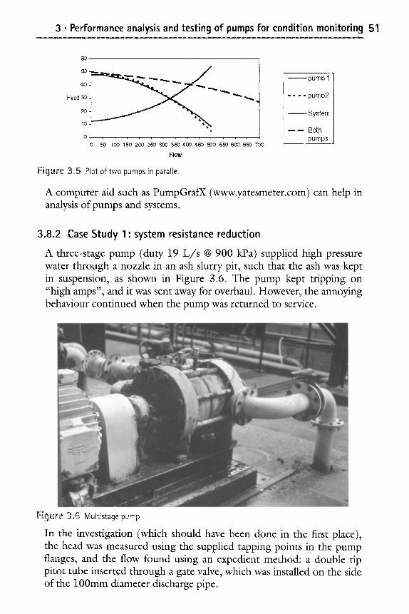
3 �9 Performance analysis and testing of pumps for condition monitoring 51
60
50
Head 30
20
10
0
0 50 100 150 200 250 300 350 400 450 500 550 600 650 700
Flow
------pump 1
. . . . pump2
- - ~ - System
- - - Both pumps
F i g u r e 3 , 5 Plot of two pumps in parallel
A computer aid such as PumpGrafX (www.yatesmeter.com) can help in analysis of pumps and systems.
3.8.2 Case Study 1" system resistance reduction
A three-stage pump (duty 19 L/s @ 900 kPa) supplied high pressure water through a nozzle in an ash slurry pit, such that the ash was kept in suspension, as shown in Figure 3.6. The pump kept tripping on "high amps", and it was sent away for overhaul. However, the annoying behaviour continued when the pump was returned to service.
Figure 3,,6 Multistage pump
In the investigation (which should have been done in the first place), the head was measured using the supplied tapping points in the pump flanges, and the flow found using an expedient method: a double tip pitot tube inserted through a gate valve, which was installed on the side of the 100mm diameter discharge pipe.
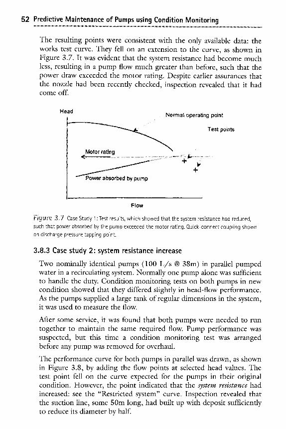
52 Predictive Maintenance of Pumps using Condition Monitoring
The resulting points were consistent with the only available data: the works test curve. They fell on an extension to the curve, as shown in Figure 3.7. It was evident that the system resistance had become much less, resulting in a pump flow much greater than before, such that the power draw exceeded the motor rating. Despite earlier assurances that the nozzle had been recently checked, inspection revealed that it had come off.
Head Normal opera~ng point
~ ~ Test ~in~
. .
Motor taring ......... �9 , , ~~" ~"'~ .......... + ,~
i ,=-, ..... i:: -.J. ! , y p i p
F l o w
Figure 3~7 Case Study 1 Test results, which showed that the system resistance had reduced, such that power absorbed by the pump exceeded the motor rating. Ouick-connect coupling shown on discharge pressure tapping point.
3.8.3 Case study 2" system resistance increase
Two nominally identical pumps (100 L / s @ 38m) in parallel pumped water in a recirculating system. Normally one pump alone was sufficient to handle the duty. Condition monitoring tests on both pumps in new condition showed that they differed slightly in head-flow performance. As the pumps supplied a large tank of regular dimensions in the system, it was used to measure the flow.
After some service, it was found that both pumps were needed to run together to maintain the same required flow. Pump performance was suspected, but this time a condition monitoring test was arranged before any pump was removed for overhaul.
The performance curve for both pumps in parallel was drawn, as shown in Figure 3.8, by adding the flow points at selected head values. The test point fell on the curve expected for the pumps in their original condition. However, the point indicated that the system resistance had increased: see the "Restricted system" curve. Inspection revealed that the suction line, some 50m long, had built up with deposit sufficiently to reduce its diameter by half.
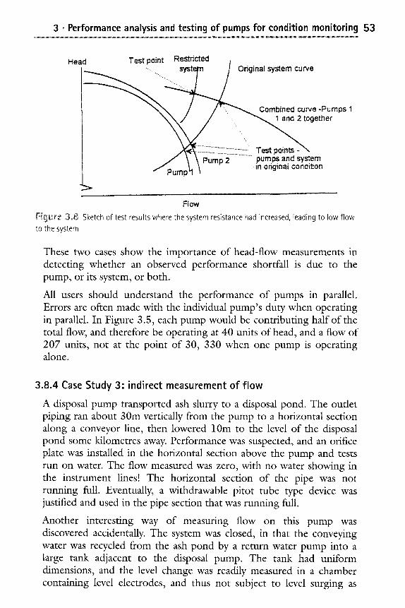
3 �9 Performance analysis and testing of pumps for condition monitoring 53
kd Test point Restricted ....................... Original system curve
Combined curve-Pumps 1 1 and 2 together
p.~ump~l \ pumps and system Pump 2 in original condition
He~
Flow Figure .~8 Sketch of test results where the system resistance had increased, leading to low flow to the system
These two cases show the importance of head-flow measurements in detecting whether an observed performance shortfall is due to the pump, or its system, or both.
All users should understand the performance of pumps in parallel. Errors are often made with the individual pump's duty when operating in parallel. In Figure 3.5, each pump would be contributing half of the total flow, and therefore be operating at 40 units of head, and a flow of 207 units, not at the point of 30, 330 when one pump is operating alone.
3.8.4 Case Study 3: indirect measurement of flow
A disposal pump transported ash slurry to a disposal pond. The outlet piping ran about 30m vertically from the pump to a horizontal section along a conveyor line, then lowered 10m to the level of the disposal pond some kilometres away. Performance was suspected, and an orifice plate was installed in the horizontal section above the pump and tests run on water. The flow measured was zero, with no water showing in the instrument lines! The horizontal section of the pipe was not running full. Eventually, a withdrawable pitot tube type device was justified and used in the pipe section that was running full.
Another interesting way of measuring flow on this pump was discovered accidentally. The system was closed, in that the conveying water was recycled from the ash pond by a return water pump into a large tank adjacent to the disposal pump. The tank had uniform dimensions, and the level change was readily measured in a chamber containing level electrodes, and thus not subject to level surging as
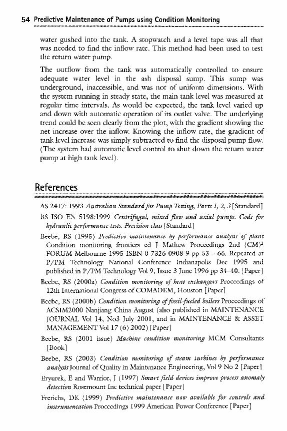
54 Predictive Maintenance of Pumps using Condition Monitoring
water gushed into the tank. A stopwatch and a level tape was all that was needed to find the inflow rate. This method had been used to test the return water pump.
The outflow from the tank was automatically controlled to ensure adequate water level in the ash disposal sump. This sump was underground, inaccessible, and was not of uniform dimensions. With the system running in steady state, the main tank level was measured at regular time intervals. As would be expected, the tank level varied up and down with automatic operation of its outlet valve. The underlying trend could be seen clearly from the plot, with the gradient showing the net increase over the inflow. Knowing the inflow rate, the gradient of tank level increase was simply subtracted to find the disposal pump flow. (The system had automatic level control to shut down the return water pump at high tank level).
References
AS 2417:1993 Australian Standard for Pump Testing, Parts 1, 2, 3 [Standard]
BS ISO EN 5198:1999 Centrifugal, mixed flow and axial pumps. Code for hydraulic performance tests. Precision class [Standard]
Beebe, RS (1995) Predictive maintenance by performance analysis of plant Condition monitoring frontiers ed J Mathew Proceedings 2nd (CM) 2 FORUM Melbourne 1995 ISBN 0 7326 0908 9 pp 53 - 66. Repeated at P/PM Technology National Conference Indianapolis Dec 1995 and published in P /PM Technology Vol 9, Issue 3 June 1996 pp 34-40. [Paper]
Beebe, RS (2000a) Condition monitoring of heat exchangers Proceedings of 12th International Congress of COMADEM, Houston [Paper]
Beebe, RS (2000b) Condition monitoring of fossil-fueled boilers Proceedings of ACSIM2000 Nanjiang China August (also published in MAINTENANCE JOURNAL Vol 14, No3 July 2001, and in MAINTENANCE & ASSET MANAGEMENT Vol 17 (6) 2002) [Paper]
Beebe, RS (2001 issue) Machine condition monitoring MCM Consultants [Book]
Beebe, RS (2003) Condition monitoring of steam turbines by performance analysis Journal of Quality in Maintenance Engineering, Vol 9 No 2 [Paper]
Eryurek, E and Warrior, J (1997) Smart field devices improve process anomaly detection Rosemount Inc technical paper [Paper]
Frerichs, DK (1999) Predictive maintenance now available for controls and instrumentation Proceedings 1999 American Power Conference [Paper]
3 �9 Performance analysis and testing of pumps for condition monitoring 55
Hines, JW; Gribok, A and Rasmussen, B (2001) On-line sensor calibration verification: "a survey" Proceedings of 14th International Congress of COMADEM, Elsevier [Paper]
International Standards Organisation: ISO5167-1.1997 Measurement offluid flow by means of orifice plates, nozzles and venturi tubes inserted in circular cross-section conduits running full (1997) [Standard]
POWER July 1961, page 187 [Article] Szanyi, R, Raterman, M, Eryurek, E (2003) Diagnostics capabilities of
FOUNDATION fieldbus pressure transmitters Hydrocarbon Processing April [Article]
www.assetmax.hispec.com [Website]
www.pepse.com [Website]
www.techsys-corp.com [Website] www.smartsignal, com/upload/appnotes/05.29.2003_Reactor%20 Pump %20A
pp6.pdf [Website] Yedidiah, S (1996) Centrifugal Pump Users Guidebook Chapman & Hall
[Book]
Performance analysis and its application to opti raise ti me for overhaul .~ The Head-Flow test at duty point @ The Shut-off Head method for monitoring of pumps @ How to calculate the optimum time for overhaul @ Optimisation using shut-off head test results @ Example to try
4.1. The Head-Flow test at duty point
Head-flow measurement can be used for all pumps where flow, or a repeatable indicator of it, can be measured. As shown in Chapter 3, this test detects pump internal deterioration as well as any changes in system resistance, or both. Complete Head-Flow-Power tests according to a Standard (such as AS 2417:1993) are rarely needed for monitoring. The Standard would need to be followed if acceptance tests are to be performed. A plant owner may require these if a new pump has not been tested at site speed and temperature in the manufacturer's works, or if the predicted pump performance has been based on model tests.
4.1.1 Duty point test: pumps in combinations
At a major power plant, each boiler-turbine generating unit has 3 x 50%, constant speed, 10 or l 1-stage boiler feed pumps. The initial condition monitoring method used for testing was to set a constant unit generation and run each combination of pumps in pairs. The combined feedwater flow and supply header pressure were noted from the service instruments. Three test points would therefore be obtained, and if one of the pumps was in worse condition than the others, the two test points containing that pump would be lower than the other point. This method is simple, and does not require calibration of
4 . Performance analysis and its application to optimise time for overhaul 57
instruments as they can be quite reasonably assumed to remain in constant calibration during the short period of the tests. However, if all the pumps degrade at the same rate, this method would not be satisfactory.
When two pumps of nominally the same characteristics are operated in parallel, similar motor currents would be expected. If after some service, a difference occurs between the motor currents, degradation in condition of one of the pumps can be expected. The worn pump may draw a lower current, or a higher current, depending on the type of wear and the control system. (See Section 5.6 for an example).
4.1.2 Full Head-FI0w test
As the combination method was not able to be used when there were only two of the pumps available for service, the next method applied was to give each individual pump a full head-flow test. This method is still used, but only to obtain the new datum curve when an overhauled pump is installed. Each pump and location tends to have its own unique performance curve, and having two spare pumps means that any location has had more than one or two different pumps installed. Note is taken of serial numbers.
Test instrumentation is installed: pressure gauges and a differential pressure transducer across the suction orifice plate (provided to initiate the automatic recirculation system for pump low flow protection), and a clip-on ammeter at the motor control cubicle. The pump is set to manual control, and throttled manually on the discharge valve to obtain a series of test points. In the development stages, the flow would reach the low flow setting, whereupon the minimum flow leakoffvalve would open, suddenly increasing pump flow and causing much noise! The pump discharge valve would then be opened and the pump returned to service.
This method was unpopular with the operators who had to work the valve, and if there were only two pumps available, could only be done if unit generation reduction was allowable and pre-arranged.
4.1.3 Head-Flow test at duty point
In the development stages, it was eventually realised that the test merely proved what was already known: that when the pump was worn, the Head-Flow curve effectively moved towards the left axis an amount equal to the internal leakage (see Chapter 2). A test at around the normal operating point would also reveal this, to the greatest clarity,
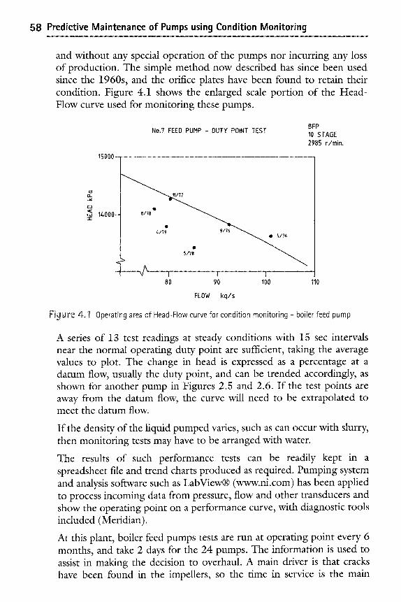
58 Predictive Maintenance of Pumps using Condition Monitoring
and without any special operation of the pumps nor incurring any loss of production. The simple method now described has since been used since the 1960s, and the orifice plates have been found to retain their condition. Figure 4.1 shows the enlarged scale portion of the Head- Flow curve used for monitoring these pumps.
s <
t/,000-
No.7 FEED PUHP - DUTY POINT TEST
8/78 e " - - . ~ / 7 7 �9
~f79 �9 6./76
"
5178
i .................. X/~ ...................... I ........................................... I ...................................... I ...............................................
80 90 100
15000 ~~. . ,~ . . . . . , ,
BFP 10 STAGE 2985 rlmin.
110
FLOW kgts
Figure 4~ I Operating area of Head-Flow curve for condition monitoring - boiler feed pump
A series of 13 test readings at steady conditions with 15 sec intervals near the normal operating duty point are sufficient, taking the average values to plot. The change in head is expressed as a percentage at a datum flow, usually the duty point, and can be trended accordingly, as shown for another pump in Figures 2.5 and 2.6. If the test points are away from the datum flow, the curve will need to be extrapolated to meet the datum flow.
If the density of the liquid pumped varies, such as can occur with slurry, then monitoring tests may have to be arranged with water.
The results of such performance tests can be readily kept in a spreadsheet file and trend charts produced as required. Pumping system and analysis software such as LabView| (www.ni.com) has been applied to process incoming data from pressure, flow and other transducers and show the operating point on a performance curve, with diagnostic tools included (Meridian).
At this plant, boiler feed pumps tests are run at operating point every 6 months, and take 2 days for the 24 pumps. The information is used to assist in making the decision to overhaul. A main driver is that cracks have been found in the impellers, so the time in service is the main
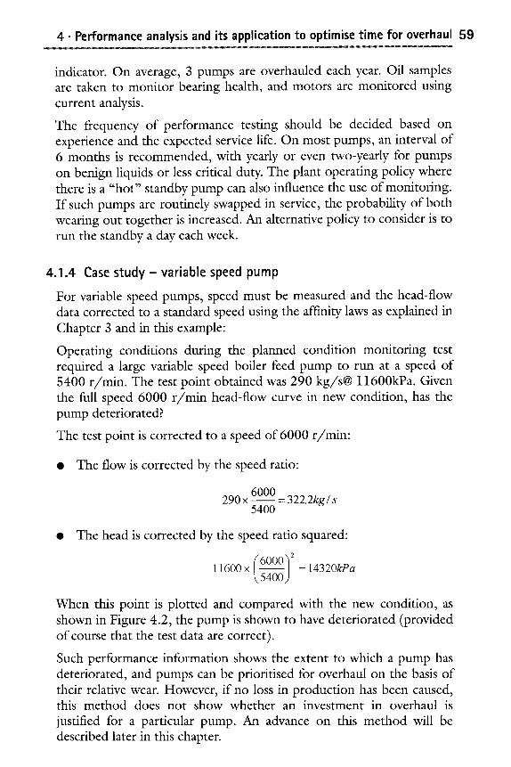
4. Performance analysis and its application to optimise time for overhaul 59
indicator. On average, 3 pumps are overhauled each year. Oil samples are taken to monitor bearing health, and motors are monitored using current analysis.
The frequency of performance testing should be decided based on experience and the expected service life. On most pumps, an interval of 6 months is recommended, with yearly or even two-yearly for pumps on benign liquids or less critical duty. The plant operating policy where there is a "hot" standby pump can also influence the use of monitoring. If such pumps are routinely swapped in service, the probability of both wearing out together is increased. An alternative policy to consider is to run the standby a day each week.
4.1.4 Case study- variable speed pump
For variable speed pumps, speed must be measured and the head-flow data corrected to a standard speed using the affinity laws as explained in Chapter 3 and in this example:
Operating conditions during the planned condition monitoring test required a large variable speed boiler feed pump to run at a speed of 5400 r /min . The test point obtained was 290 kg/s@ 11600kPa. Given the full speed 6000 r / m i n head-flow curve in new condition, has the pump deteriorated?
The test point is corrected to a speed of 6000 r /min:
�9 The flow is corrected by the speed ratio:
6000 290 x ~ - 322.2kg / s
5400
The head is corrected by the speed ratio squared:
11600 x 5400) - 14320kPa
When this point is plotted and compared with the new condition, as shown in Figure 4.2, the pump is shown to have deteriorated (provided of course that the test data are correct).
Such performance information shows the extent to which a pump has deteriorated, and pumps can be prioritised for overhaul on the basis of their relative wear. However, if no loss in production has been caused, this method does not show whether an investment in overhaul is justified for a particular pump. An advance on this method will be described later in this chapter.
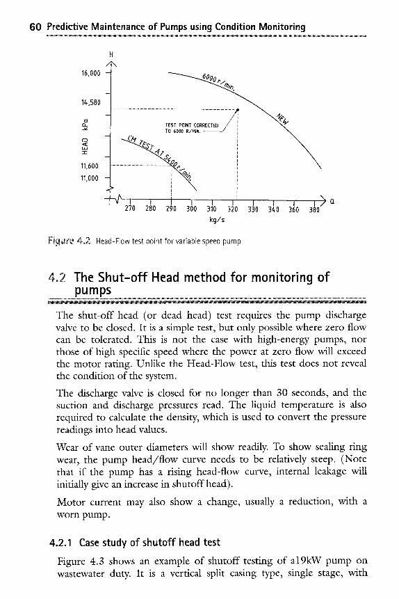
60 Predictive Maintenance of Pumps using Condition Monitoring
H / \
16.000 _ -
14.,580 _ - . . . . . . . . . . . . . . . . -~ ~ + ~ ,
_v TO 6000 R / M I N . " / I
,,,ooo F 1 '
1
- - r , ....... t' , , , , , , ,++)a 2"/0 280 290 300 310 320 330 340 360 380
kg/s
F igure 4+2 Head-Flow test point for variable speed pump
4,2 The S h u t - o f f Head method for monitor ing of pumps
The shut-off head (or dead head) test requires the pump discharge valve to be closed. It is a simple test, but only possible where zero flow can be tolerated. This is not the case with high-energy pumps, nor those of high specific speed where the power at zero flow will exceed the motor rating. Unlike the Head-Flow test, this test does not reveal the condition of the system.
The discharge valve is closed for no longer than 30 seconds, and the suction and discharge pressures read. The liquid temperature is also required to calculate the density, which is used to convert the pressure readings into head values.
Wear of vane outer diameters will show readily. To show sealing ring wear, the pump head/f low curve needs to be relatively steep. (Note that if the pump has a rising head-flow curve, internal leakage will initially give an increase in shutoff head).
Motor current may also show a change, usually a reduction, with a worn pump.
4.2.1 Case study of shutoff head test
Figure 4.3 shows an example of shutoff testing of a19kW pump on wastewater duty. It is a vertical split casing type, single stage, with
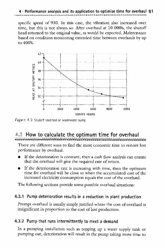
4. Performance analysis and its application to optimise time for overhaul 61
specific speed of 930. In this case, the vibration also increased over time, but this is not always so. After overhaul at 10 000h, the shutoff head returned to the original value, as would be expected. Maintenance based on condition monitoring extended time between overhauls by up to 400%.
/+2
/+0- t.LJ
k--
,,, 38
LL. LI..
o 36~ I.-- ::D 71- U3
~_ 3/+- .,r
O
< 32 I.tJ
"'~.....~ I ! j
0 2000 4000 6000 8000 10000
SERVICE HOURS
F i g u r e 4..3 Shutoff head test on wastewater pump
4+3 How to calculate the optimum time for overhaul
There are different ways to find the most economic time to restore lost performance by overhaul.
�9 If the deterioration is constant, then a cash flow analysis can ensure that the overhaul will give the required rate of return.
�9 If the deterioration rate is increasing with time, then the optimum time for overhaul will be close to when the accumulated cost of the increased electricity consumption equals the cost of the overhaul.
The following sections provide some possible overhaul situations:
4.3.1 Pump deterioration results in a reduction in plant production
Prompt overhaul is usually simply justified where the cost of overhaul is insignificant in proportion to the cost of lost production.
4.3.2 Pump that runs intermittently to meet a demand
In a pumping installation such as topping up a water supply tank or pumping out, deterioration will result in the pump taking more time to
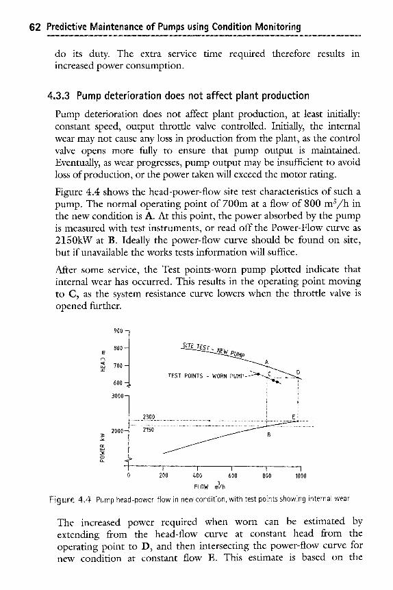
62 Predictive Maintenance of Pumps using Condition Monitoring
do its duty. The extra service increased power consumption.
time required therefore results in
4.3.3 Pump deterioration does not affect plant production
Pump deterioration does not affect plant production, at least initially: constant speed, output throttle valve controlled. Initially, the internal wear may not cause any loss in production from the plant, as the control valve opens more fially to ensure that pump output is maintained. Eventually, as wear progresses, pump output may be insufficient to avoid loss of production, or the power taken will exceed the motor rating.
Figure 4.4 shows the head-power-flow site test characteristics of such a pump. The normal operating point of 700m at a flow of 800 mS/h in the new condition is A. At this point, the power absorbed by the pump is measured with test instruments, or read off the Power-Flow curve as 2150kW at B. Ideally the power-flow curve should be found on site, but if unavailable the works tests information will suffice.
After some service, the Test points-worn pump plotted indicate that internal wear has occurred. This results in the operating point moving to C, as the system resistance curve lowers when the throttle valve is opened further.
TES
900
800 E
r ~
700
60O
I i 3000- i
2300 ~ El
2000- - ....... 2~ ....... - - - - ~ ~ B . . . . . . . . . . . . t ............ i 1 . . . . . t . . . . . . . . . . . . . . . . . . . . . . . . . . . i
0 200 r 600 800 1000
FLOW m31h
F i g u r e 4 . 4 Pump head-power-f low in new condition, with test points showing internal wear
The increased power required when worn can be estimated by extending from the head-flow curve at constant head from the operating point to D, and then intersecting the power-flow curve for new condition at constant flow E. This estimate is based on the
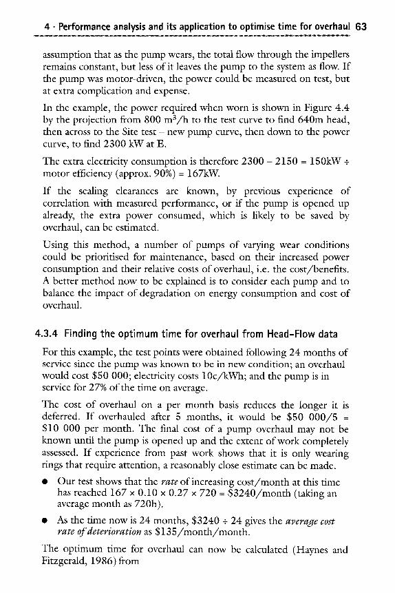
4- Performance analysis and its application to optimise time for overhaul 63
assumption that as the pump wears, the total flow through the impellers remains constant, but less of it leaves the pump to the system as flow. If the pump was motor-driven, the power could be measured on test, but at extra complication and expense.
In the example, the power required when worn is shown in Figure 4.4 by the projection from 800 m3/h to the test curve to find 640m head, then across to the Site t e s t - new pump curve, then down to the power curve, to find 2300 kW at E.
The extra electricity consumption is therefore 2300 - 2150 = 150kW + motor efficiency (approx. 90%) - 167kW.
If the sealing clearances are known, by previous experience of correlation with measured performance, or if the pump is opened up already, the extra power consumed, which is likely to be saved by overhaul, can be estimated.
Using this method, a number of pumps of varying wear conditions could be prioritised for maintenance, based on their increased power consumption and their relative costs of overhaul, i.e. the cost/benefits. A better method now to be explained is to consider each pump and to balance the impact of degradation on energy consumption and cost of overhaul.
4.3.4 Finding the optimum time for overhaul from Head-Flow data
For this example, the test points were obtained following 24 months of service since the pump was known to be in new condition; an overhaul would cost $50 000; electricity costs 10c/kWh; and the pump is in service for 27% of the time on average.
The cost of overhaul on a per month basis reduces the longer it is deferred. If overhauled after 5 months, it would be $50 0 0 0 / 5 - $10 000 per month. The final cost of a pump overhaul may not be known until the pump is opened up and the extent of work completely assessed. If experience from past work shows that it is only wearing rings that require attention, a reasonably close estimate can be made.
�9 Our test shows that the rate of increasing cos t /month at this time has reached 167 x 0.10 x 0.27 x 720 = $ 3 2 4 0 / m o n t h (taking an average month as 720h).
�9 As the time now is 24 months, $3240 + 24 gives the average cost rate of deterioration as $ 1 3 5 / m o n t h / m o n t h .
The optimum time for overhaul can now be calculated (Haynes and Fitzgerald, 1986) from
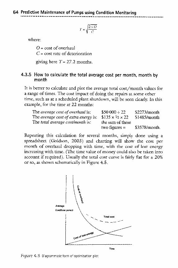
64 Predictive Maintenance of Pumps using Condition Monitoring
~/2xO T= C
where"
O = cost of overhaul C = cost rate of deterioration
giving here T= 27.2 months.
4.3.5 How to calculate the total average cost per month, month by month
It is better to calculate and plot the average total cos t /month values for a range of times. The cost impact of doing the repairs at some other time, such as at a scheduled plant shutdown, will be seen clearly. In this example, for the time at 22 months:
The average cost of overhaul is" The average cost of extra energy is" The total average cost~month is:
$50 000 + 22 $135 x 1/2 x 22 the sum of these two figures-
$2273/month $1485/month
$3578/month.
Repeating this calculation for several months, simply done using a spreadsheet (Goldson, 2003) and charting will show the cost per month of overhaul dropping with time, with the cost of lost energy increasing with time. (The time value of money could also be taken into account if required). Usually the total cost curve is fairly flat for + 20% or so, as shown schematically in Figure 4.5.
O \
Average Cost/time period ~ \
\ ] ~ " .... Total cost
Time
Figure 4,5 Diagrammatic form of optimisation plot
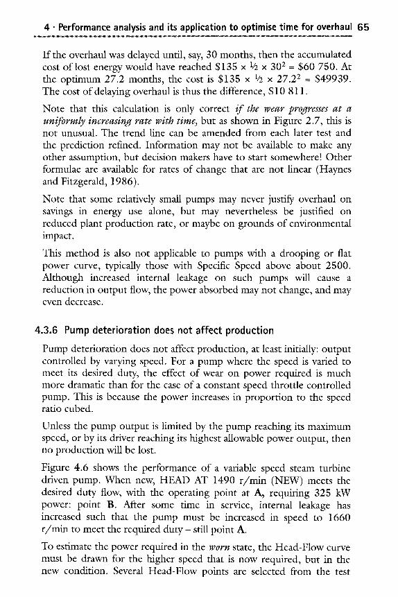
4. Performance analysis and its application to optimise time for overhaul 65
If the overhaul was delayed until, say, 30 months, then the accumulated cost of lost energy would have reached $135 x 1/2 x 302 = $60 750. At the optimum 27.2 months, the cost is $135 x 1/2 x 27.22 = $49939. The cost of delaying overhaul is thus the difference, $10 811.
Note that this calculation is only correct i f the wear progresses at a uniformly increasing rate with time, but as shown in Figure 2.7, this is not unusual. The trend line can be amended from each later test and the prediction refined. Information may not be available to make any other assumption, but decision makers have to start somewhere! Other formulae are available for rates of change that are not linear (Haynes and Fitzgerald, 1986).
Note that some relatively small pumps may never justify overhaul on savings in energy use alone, but may nevertheless be justified on reduced plant production rate, or maybe on grounds of environmental impact.
This method is also not applicable to pumps with a drooping or flat power curve, typically those with Specific Speed above about 2500. Although increased internal leakage on such pumps will cause a reduction in output flow, the power absorbed may not change, and may even decrease.
4.3.6 Pump deterioration does not affect production
Pump deterioration does not affect production, at least initially: output controlled by varying speed. For a pump where the speed is varied to meet its desired duty, the effect of wear on power required is much more dramatic than for the case of a constant speed throttle controlled pump. This is because the power increases in proportion to the speed ratio cubed.
Unless the pump output is limited by the pump reaching its maximum speed, or by its driver reaching its highest allowable power output, then no production will be lost.
Figure 4.6 shows the performance of a variable speed steam turbine driven pump. When new, HEAD AT 1490 r / m i n (NEW) meets the desired duty flow, with the operating point at A, requiting 325 kW power: point B. After some time in service, internal leakage has increased such that the pump must be increased in speed to 1660 r / m i n to meet the required duty - still point A.
To estimate the power required in the worn state, the Head-Flow curve must be drawn for the higher speed that is now required, but in the new condition. Several Head-Flow points are selected from the test
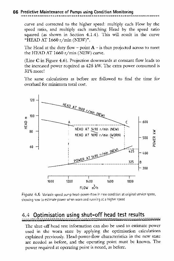
66 Predictive Maintenance of Pumps using Condition Monitoring
curve and corrected to the higher speed: multiply each Flow by the speed ratio, and multiply each matching Head by the speed ratio squared (as shown in Section 4.1.4). This will result in the curve "HEAD AT 1660 r /min (NEW)".
The Head at the duty f low- point A - is then projected across to meet the HEAD AT 1660 r /min (NEW) curve.
(Line C in Figure 4.6). Projection downwards at constant flow leads to the increased power required as 425 kW. The extra power consumed is 31% more!
The same calculations as before are followed to find the time for overhaul for minimum total cost.
EE
C3
t j . j Z
t20 -
100 -
8 0 -
60 -
HEAD AT 1490 r/min (NEW) ,
HEAD AT 1690 r/rain (WORN) t I
+ ', !
-600
- 500
- 4 0 0
B
- 300
OC LI.I
3: O (3.
! " I . . . . . I ! I
1000 1200 1400 1600 1800
FLOW m3/h
Fig[~re 4.6 Variable-speed pump head-power-flow in new condition at original service speed,
showing how to estimate power when worn and running at a higher speed
4.40ptimisation using shut-off head test results
The shut-off head test information can also be used to estimate power used in the worn state by applying the optimisation calculations explained previously. Head-power-flow characteristics in the new state are needed as before, and the operating point must be known. The power required at operating point is noted, as before.
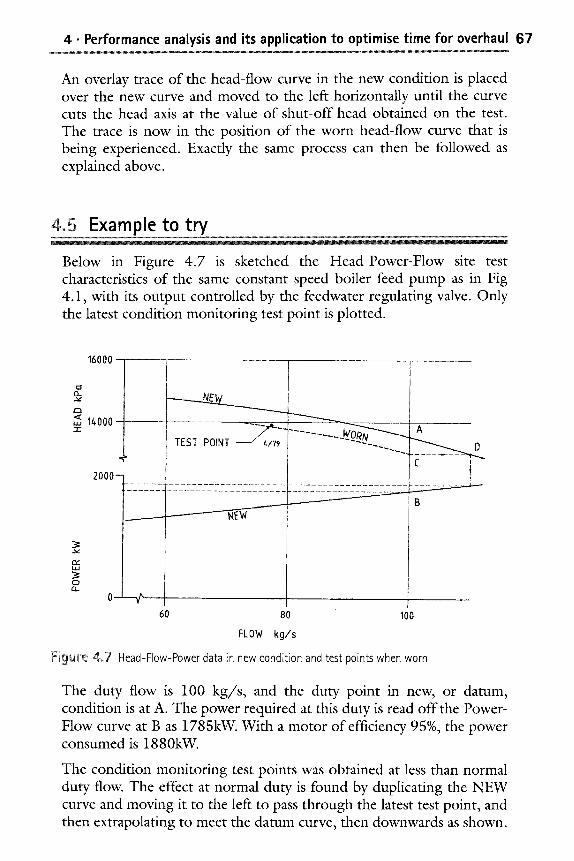
4. Performance analysis and its application to optimise time for overhaul 67
An overlay trace of the head-flow curve in the new condition is placed over the new curve and moved to the left horizontally until the curve cuts the head axis at the value of shut-off head obtained on the test. The trace is now in the position of the worn head-flow curve that is being experienced. Exactly the same process can then be followed as explained above.
4~ Example to try
Below in Figure 4.7 is sketched the Head-Power-Flow site test characteristics of the same constant speed boiler feed pump as in Fig 4.1, with its output controlled by the feedwater regulating valve. Only the latest condition monitoring test point is plotted.
16000 --
1/.000- ~ . . . . .
TEST POINT . ~ " s
2ooo- L . . . . . . . .
~ B
o, r . . . . . . . 60 80 . 100
FLOW kg/s
F ] g u ~ ' e 4~ Head-Flow-Power data in new condition and test points when worn
The duty flow is 100 kg/s , and the duty point in new, or datum, condition is at A. The power required at this duty is read off the Power- Flow curve at B as 1785kW. With a motor of efficiency 95%, the power consumed is 1880kW.
The condition monitoring test points was obtained at less than normal duty flow. The effect at normal duty is found by duplicating the NEW curve and moving it to the left to pass through the latest test point, and then extrapolating to meet the datum curve, then downwards as shown.
68 Predictive Maintenance of Pumps using Condition Monitoring
(The system resistance curve lowers when the throttle valve is opened further). The power estimated to be required in the worn condit ion is thus 1895kW.
The cost of an overhaul is estimated at $50 000. At this time, the cost of extra used-in-station electricity is 2 c / k W h , and the pump runs for 90% of the time on average.
Calculate the increased electricity consumption"
? - ? = ? + 0.95 = ?kW
�9 Calculate the current extra cost of electricity:
? x ? x ? x 720 = ?S /month .
(Take a mon th as 720h on average).
�9 Calculate the average cost rate of deterioration:
$ ? + gives $ ? / m o n t h / m o n t h .
�9 Calculate the op t imum time for overhaul from T - ~ J 2 0
where" V C O--- cost of overhaul-- .9 C-- cost rate of deterioration -- .9 giving here T= .9 months
Calculate the extra cost incurred if the overhaul is to be deferred until 36 months since the last overhaul:
�9 Find the accumulated cost of extra used-in-station energy to the calculated optimum time from:
$.9 X 1/2 X 9 2 = $.9
�9 Find the accumulated cost of extra used-in-station energy to 36 months:
$.9 • 1/2 • 362= $?
The answer is given at the end of this chapter.
References
AS 2417"1993 Australian Standard for Pump Testing, Parts 1, 2, 3 [Standard]
BS ISO EN 5198"1999 Centrifugal, mixed flow and axial pumps. Code for hydraulic performance tests. Precision class [Standard]
Goldson's Rotating Machinery Coffee Shop: http://www.goldson.free- online.co.uk/programs.htm [Website]
Haynes, C J and Fitzgerald, M A (1986) Scheduling Power Plant Maintenance Using Performance Data ASME Paper 86-JPGC-Pwr-63 [Paper]
4 . Performance analysis and its application to optimise time for overhaul 69
www.meridian- engineers.com, au [Website]
www.ni.com/labview/[Website]
www.yatesmeter.com [Website]
Appendix
Example Procedure for Condition Monitoring Performance Test, kept on office computer and updated as required. Copies are printed and provided to Instrumentation Supervisor and Production Supervisor with work requests.
PLANT CONDITION MONITORING TEST PROCEDURE T.41
Jul 1999 Issued 15
Test file 6.7
I. Plant item Boiler feed pumps
2. Performance and outline data 3 x 50Olo. 4 Stages, with single-stage suction booster pump. Duty: 150kg/s @15500 kPa, water at 150degC.
Main pump: constant speed via step-up gearbox, 5800 r/min. Suction booster pump, constant speed 1485 r/min. Motor 3456kW.
Gland sealing water from condensate extraction pump discharge. Some mixes with hotwater from pump gland unloading line, most outflows to clean drains tank or surface drain.
Flow metering via orifice plate in line from booster pump to main pump (provided to initiate low flow protection). Orifice plate in gland supply line, and also in clean drains tank. Flow from thrust balance returned to pump suction.
Output control via feedwater regulating valve.
3. Test type and frequency a. Overall Performance Test at normal duty point: each 3 months, or on
request.
b. Full Performance Test - i f and as required (gland sealing inflows and outflows are measured).
c. Routine vibration measurements as detailed in vibration route files (amplitude in H-A-V directions at each bearing, spectra as detailed),
70 Predictive Maintenance of Pumps using Condition Monitoring
4. Performance Test Instrumentation: Overall Performance Test: �9 Test pressure gauges connected in parallel with panel; gauges, mounted on
stand at panel:
�9 Booster suction:O- 1500kPa �9 Main suction:O- 2500 kPa �9 Main discharge: O-20MPa
�9 Test Differential Pressure transducer, calibrated from O-60kPa, connected across leakoff initiation orifice plate. NOTE: get Production to isolate initiation circuits while transducer is connected and are bled. Do not open equalising valve with initiation circuit in service, or minimum flow device will operate.
.5. Test preparation A week prior to the test, request Instrumentation Supervisor to be install instru- mentation, and provide copy of this Procedure.
On day before, send "Application for Test" to Production Supervisor, with copy of this Procedure.
6. Test procedure a. With test pump control placed on manual, and steady conditions obtained,
take readings of instruments at regular intervals, using test sheet E41 or PDAs, co-ordinating observers as necessary.
b. Note the "feed pump common suction temperature" for the period on the DCS in the control room.
c. Ask Production to increase output of the test pump by about 5O/o on the DCS (the other pumps will be reduced automatically by the feed control system), and obtain another set of test readings.
d Ask Production to reduce output of the test pump by about 5% on the DCS, and obtain a third set of readings.
Request the test instrumentation to be transferred to the next pump, and repeat the same test process for that pump.
Repeat to obtain test points for the third pump.
g. Request removal and check calibration of test instrumentation. Specify the points at which calibration is to be done (usually 6 points, spanning the range of test readings).
7. Calculation and recording of results For each test, as applicable:
a. Download test data, and average test differential pressure readings and apply calibration to find differential pressures.
b. Using the average temperature, calculate flow from:
Main pump: W = 0.675 ~/[density (kg/m 3) x differential pressure (kPa)] kg/s
4. Performance analysis and its application to optimise time for overhaul 71
Average pressures and apply calibration corrections.
Calculate booster pump discharge pressure by adding the estimated pressure drop through the connecting pipe from: Pressure drop (kPa) = 0.0025 x Flow 2 kPa
e. Determine the Generated Pressures for both booster and main pumps.
f. Correct flows and pressures to standard water density at 150degC, and average water pressure in the pumps: multiply flows and pressures by the ration of reference density over test density (find from www.pepse.com).
g. Plot Head-Flow points on file curve, and compare with last test. Draw line of best fit through points, and extrapolate to find the value at design duty of 150kgls. Calculate the percentage reduction in head, and plot on trend graph. Note service hours since last overhaul.
h. Perform optimisation of overhaul calculations as detailed in standard file, and recommend action accordingly.
Answer for Example to try
The power required for this duty in the worn condition is scaled off the figure
by the projection from the duty flow of 100kg/s to the "worn" curve to find
13107 kPa head, then across to the "Site test-new" curve, then down to the
power-flow curve, to find 1895 kW.
The extra electricity consumption is therefore 1895 - 1785 = 110kW + motor
efficiency (95%)= 116kW.
Our test shows that the rate of increasing cos t /month has reached 116 % 0.02 % 0.9 % 720 = $1503/month . (A month has 720h on average).
As the time now is 15 months, $1503 + 15 gives the average cost rate of
deterioration as $ 1 0 0 / m o n t h / m o n t h .
The optimum time for overhaul calculated from T - / 2 0 C
gives T= 32 months
If the overhaul was delayed until, say, 36 months, then the accumulated cost of
lost energy would have reached $100 x 1/2 x 362 = $64800.
At 32 months, the cost is $100 x 1/2 x 322 = $51200. The cost of delaying overhaul is thus the difference, $13600.
Other methods of performance analysis for pump condition monitoring i Introduction: simple parameters m Measurement of the balance device leakoff flow @ Case Study: balance leakoffflow method @ Some other experience with the balance-flow method @ Thermometric testing @ Head-Power Characteristics
5~ Introduction" simple parameters
Although it is considered that the methods described in Chapter 4 arc the most generally applicable, there are other methods that may be more appropriate in given circumstances. It may not be possible to mcasure flow, and special facilities may be provided enabling other methods. An example in the case of variable speed pumps is to monitor the speed routinely. If the system has not changed, then pump degradation will result in a higher speed to meet the required duty.
An installation may have several pumps in parallel, with each switched on automatically in turn to meet a variable duty (such as in town water supply). Over a period, if it may be assumed that the total duty is relatively constant, it may be assumed that if a particular pump's running hours are greater than its companion machines, then its condition is worse. Allowance for different pump sizes would of course be needed.
It is not suggested that the overhaul decision be based on the above methods alone, but they can be useful as screening to indicate when a specific test is required.
This Chapter covers some other available methods.
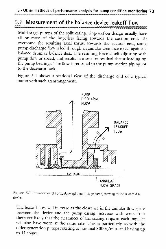
5 �9 Other methods of performance analysis for pump condition monitoring 73
5~ Measurement of the balance device leakoff flow
Multi-stage pumps of the split casing, ring-section design usually have all or most of the impellers facing towards the suction end. To overcome the resulting axial thrust towards the suction end, some pump discharge flow is led through an annular clearance to act against a balance drum or balance disk. The resulting force is self-adjusting with pump flow or speed, and results in a smaller residual thrust loading on the pump bearings. The flow is returned to the pump suction piping, or to the deaerator tank.
Figure 5.1 shows a sectional view of the discharge end of a typical pump with such an arrangement.
PUMP DISCHARGE
/ \ FLOW
?
~ V/,///~ BALANCE ~///r#////~t -~ LEAKOFF ~/ I e,, / I FLOW
. , . ~ v/4////,Q
Z .......
- CENTRELINE _ ~ .......
L ANNULAR FLOW SPACE
Figure 5,,I Cross-section of horizontally-split multi-stage pump, showing thrust balance disk device
The leakoff flow will increase as the clearance in the annular flow space between the device and the pump casing increases with wear. It is therefore likely that the clearances of the sealing tings at each impeller will also have worn at the same rate. This is particularly so with the older generation pumps rotating at nominal 3000r /min , and having up to 11 stages.
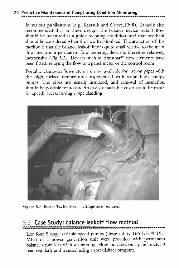
74 Predictive Maintenance of Pumps using Condition Monitoring
In various publications (e.g. Karassik and Grieve,1998), Karassik also recommended that in these designs the balance device leakoff flow should be measured as a guide to pump condition, and that overhaul should be considered when the flow has doubled. The attraction of this method is that the balance leakoff line is quite small relative to the main flow line, and a permanent flow metering device is therefore relatively inexpensive (Fig 5.2). Devices such as Annubar T~ flow elements have been fitted, relaying the flow to a panel meter or the control room
Portable clamp-on flowmeters are now available for use on pipes with the high surface temperatures experienced with some high energy pumps. The pipes are usually insulated, and removal of insulation should be possible for access. An easily detachable cover could be made for speedy access through pipe cladding.
Figure 5,2 Balance flow line from a multistage boiler feed pump
5~ Case Study" balance leakoff flow method
The four 5-stage variable speed pumps (design duty 166 L / s @ 19.1 MPa) of a power generation unit were provided with permanent balance drum leakoff flow metering. Flow indicated on a panel meter is read regularly and trended using a spreadsheet program.
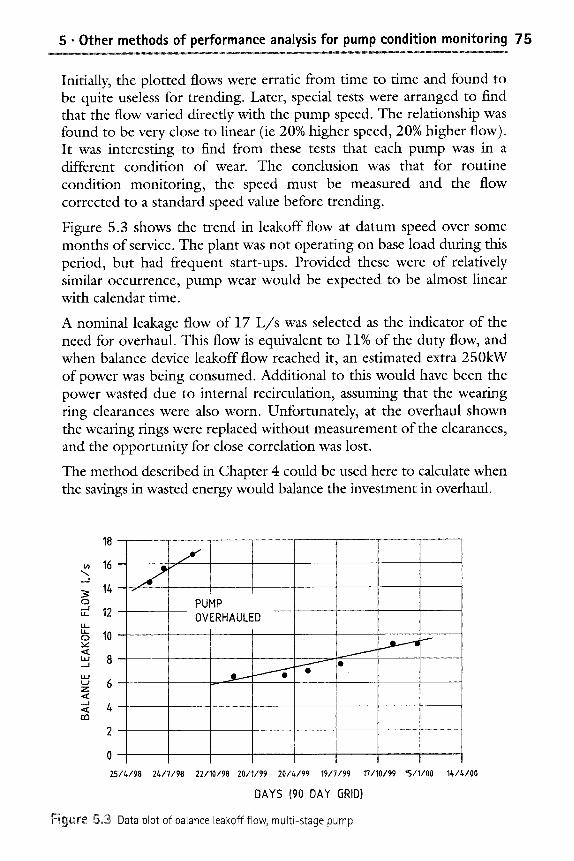
5 �9 Other methods of performance analysis for pump condition monitoring 75
Initially, the plotted flows were erratic from time to time and found to be quite useless for trending. Later, special tests were arranged to find that the flow varied directly with the pump speed. The relationship was found to be very close to linear (ie 20% higher speed, 20% higher flow). It was interesting to find from these tests that each pump was in a different condition of wear. The conclusion was that for routine condition monitoring, the speed must be measured and the flow corrected to a standard speed value before trending.
Figure 5.3 shows the trend in leakoff flow at datum speed over some months of service. The plant was not operating on base load during this period, but had frequent start-ups. Provided these were of relatively similar occurrence, pump wear would be expected to be almost linear with calendar time.
A nominal leakage flow of 17 L / s was selected as the indicator of the need for overhaul. This flow is equivalent to 11% of the duty flow, and when balance device leakoff flow reached it, an estimated extra 250kW of power was being consumed. Additional to this would have been the power wasted due to internal recirculation, assuming that the wearing ring clearances were also worn. Unfortunately, at the overhaul shown the wearing rings were replaced without measurement of the clearances, and the opportunity for close correlation was lost.
The method described in Chapter 4 could be used here to calculate when the savings in wasted energy would balance the investment in overhaul.
18
16 . , J
c~
u_ 12 U_ o 10
"' 8 __1
~ 6 z
_.1
J
PUMP OVERHAULED
, .
. , ,
. . . . . . . . . . . .
25//,/98 2/,/7/98 22/10/98 2011/99
~ o o
2016/99 19/7/99 17/10/99 15/I/00
DAYS (90 DAY GRID)
Figure 5~ Data plot of balance leakoff flow, multi-stage pump
14/4/00
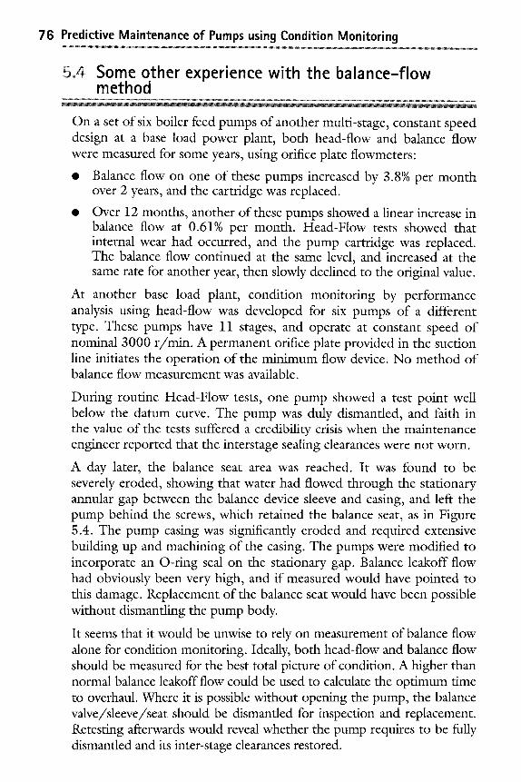
76 Predictive Maintenance of Pumps using Condition Monitoring
5~ Some other experience with the balance-flow method
On a set of six boiler feed pumps of another multi-stage, constant speed design at a base load power plant, both head-flow and balance flow were measured for some years, using orifice plate flowmeters:
�9 Balance flow on one of these pumps increased by 3.8% per month over 2 years, and the cartridge was replaced.
�9 Over 12 months, another of these pumps showed a linear increase in balance flow at 0.61% per month. Head-Flow tests showed that internal wear had occurred, and the pump cartridge was replaced. The balance flow continued at the same level, and increased at the same rate for another year, then slowly declined to the original value.
At another base load plant, condition monitoring by performance analysis using head-flow was developed for six pumps of a different type. These pumps have 11 stages, and operate at constant speed of nominal 3000 r /min. A permanent orifice plate provided in the suction line initiates the operation of the minimum flow device. No method of balance flow measurement was available.
During routine Head-Flow tests, one pump showed a test point well below the datum curve. The pump was duly dismantled, and faith in the value of the tests suffered a credibility crisis when the maintenance engineer reported that the interstage sealing clearances were not worn.
A day later, the balance seat area was reached. It was found to be severely eroded, showing that water had flowed through the stationary annular gap between the balance device sleeve and casing, and left the pump behind the screws, which retained the balance seat, as in Figure 5.4. The pump casing was significantly eroded and required extensive building up and machining of the casing. The pumps were modified to incorporate an O-ring seal on the stationary gap. Balance leakoff flow had obviously been very high, and if measured would have pointed to this damage. Replacement of the balance seat would have been possible without dismantling the pump body.
It seems that it would be unwise to rely on measurement of balance flow alone for condition monitoring. Ideally, both head-flow and balance flow should be measured for the best total picture of condition. A higher than normal balance leakoff flow could be used to calculate the optimum time to overhaul. Where it is possible without opening the pump, the balance valve/sleeve/seat should be dismantled for inspection and replacement. Retesting afterwards would reveal whether the pump requires to be fully dismantled and its inter-stage clearances restored.
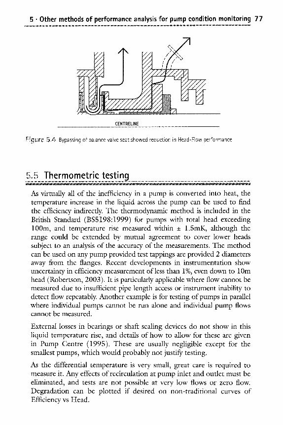
5 �9 Other methods of performance analysis for pump condition monitoring 77
I, / ",,"
l ......
~ . , t " P - - - ~ ~ .(.. (k,~ " ,-~,\'%X~A
CENTRELtNE
Figure 5,4 Bypassing of balance valve seat showed reduction in Head-Flow performance
5~ Thermometric testing
As virtually all of the inefficiency in a pump is converted into heat, the temperature increase in the liquid across the pump can be used to find the efficiency indirectly. The thermodynamic method is included in the British Standard (BS5198:1999) for pumps with total head exceeding 100m, and temperature rise measured within _+ 1.SmK, although the range could be extended by mutual agreement to cover lower heads subject to an analysis of the accuracy of the measurements. The method can be used on any pump provided test tappings are provided 2 diameters away from the flanges. Recent developments in instrumentation show uncertainty in efficiency measurement of less than 1%, even down to 10m head (Robertson, 2003). It is particularly applicable where flow cannot be measured clue to insufficient pipe length access or instrument inability to detect flow repeatably. Another example is for testing of pumps in parallel where individual pumps cannot be run alone and individual pump flows cannot be measured.
External losses in bearings or shaft sealing devices do not show in this liquid temperature rise, and details of how to allow for these are given in Pump Centre (1995). These are usually negligible except for the smallest pumps, which would probably not justify testing.
As the differential temperature is very small, great care is required to measure it. Any effects of recirculation at pump inlet and outlet must be eliminated, and tests are not possible at very low flows or zero flow. Degradation can be plotted if desired on non-traditional curves of Efficiency vs Head.
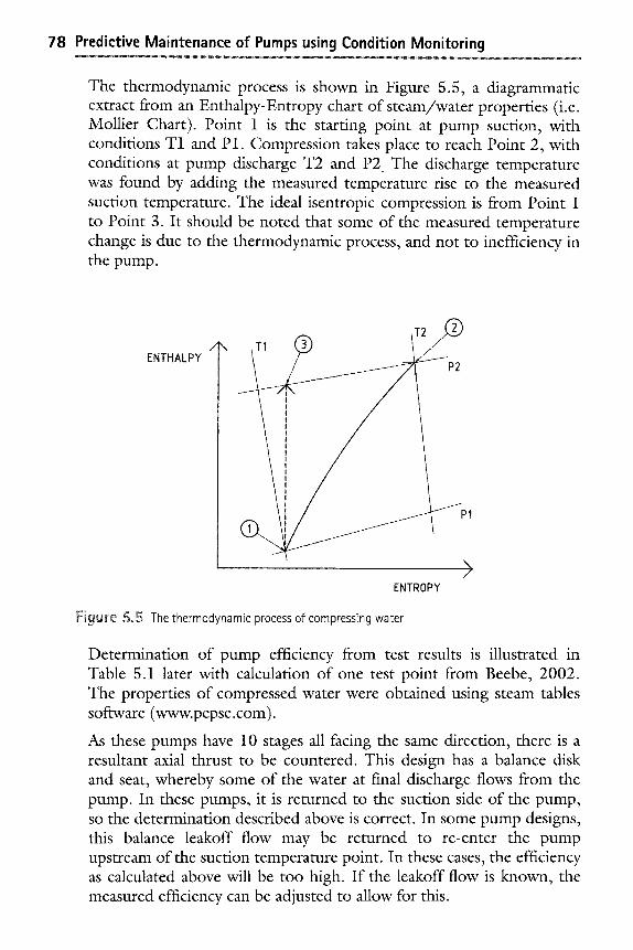
78 Predictive Maintenance of Pumps using Condition Monitoring
The thermodynamic process is shown in Figure 5.5, a diagrammatic extract from an Enthalpy-Entropy chart of steam/water properties (i.e. Mollier Chart). Point 1 is the starting point at pump suction, with conditions T1 and P1. Compression takes place to reach Point 2, with conditions at pump discharge T2 and P2 The discharge temperature was found by adding the measured temperature rise to the measured suction temperature. The ideal isentropic compression is from Point 1 to Point 3. It should be noted that some of the measured temperature change is due to the thermodynamic process, and not to inefficiency in the pump.
ENTHALPY
I T 2 TI A .._.
PI
. . . . . . . .
ENTROPY
F igure 5 ,5 The thermodynamic process of compressing water
Determination of pump efficiency from test results is illustrated in Table 5.1 later with calculation of one test point from Beebe, 2002. The properties of compressed water were obtained using steam tables software (www.pepse.com).
As these pumps have 10 stages all facing the same direction, there is a resultant axial thrust to be countered. This design has a balance disk and seat, whereby some of the water at final discharge flows from the pump. In these pumps, it is returned to the suction side of the pump, so the determination described above is correct. In some pump designs, this balance leakoff flow may be returned to re-enter the pump upstream of the suction temperature point. In these cases, the efficiency as calculated above will be too high. If the leakoff flow is known, the measured efficiency can be adjusted to allow for this.
5 �9 Other methods of performance analysis for pump condition monitoring 79
Developments in the mining industry in South Africa (Whillier, 1972) led to a simple empirical equation applicable to pumps on water at up to 54~ A correction is included to allow for the very small temperature rise that occurs as a result of the changes in thermo- dynamic properties with increase in pressure (see example earlier).
With Total Head in kPa, and temperatures in ~
Efficiency (decimal)- 100
[1-0 O03(In le t temp-2) +4160 Temp rise " Total H e a d .]
Commercially available devices are widely used in the water industry in the UK and elsewhere (e.g. www.aems.co.uk and www.pumpmonitor. com), and recent applications to large pumps are of interest (Yates and Kumar, 1999; Thorne and Neal, 1996). To minimise the effects of any recirculation, the tapping points for the installation of pressure/ temperature probes are required at two diameters away from the pump suction and discharge pump flanges, as for the traditional precision class tests. Furthermore, the temperatures must be measured in the flowing stream.
If the motor power is measured from the motor input wiring, the motor losses can be assessed, and the power absorbed by the pump computed. By combining this with the pressure and temperature rise data, the pump flow can be calculated. The test results are shown in real time, and graphs of efficiency versus flow can be obtained.
Most pumps in industry do not have tappings other than at the flanges, and to add extra tappings in a typical power plant with over 100 pumps is a disincentive to apply the thermodynamic method, particularly where the Head-Flow method has proven satisfactory. The thermo- dynamic method would be more attractive economically if no extra tapping points were required. A test is reported where temperatures were also measured at the pump flanges, and gave a different result for efficiency (Thorne and Neal, 1996). These points may however be satisfactory for routine monitoring, as with Head-Flow tests.
Temperatures measured on the pipe surface have been found to relate closely to that of the liquid flowing for obtaining differential temperature (Murray et al 1989). Experiments conducted on some boiler feed pumps without the use of special tappings showed promise (Beebe, 2002). An electronic differential temperature device was arranged to measure suction and discharge pipe surface temperatures on tests with water at 127~ Insulation was applied to ensure that surface temperature was close to that of the water flowing in the pipe.
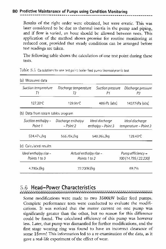
80 Predictive Maintenance of Pumps using Condition Monitoring
Results of the right order were obtained, but were erratic. This was later considered to be due to thermal inertia in the pump and piping, and if flow is varied, an hour should be allowed between tests. This application of the method shows promise for routine monitoring at reduced cost, provided that steady conditions can be arranged before test readings are taken.
The following table shows the calculation of one test point during these tests.
Table 5o 1 Calculations for one test point: boiler feed pump thermodynamic test
(a) Measured data
Suction temperature Discharge temperature Suction pressure
T1 T2 P1 Discharge pressure
P2
127.20oC 129.95oC 486kPa (abs) 14377kPa (abs)
(b) Data from steam tables program
Suction enthalpy- Discharge enthalpy Ideal discharge Ideal discharge
Point 1 - Point 2 enthalpy- Point 3 temperature - Point 3
534.47kJ/kg 5 5 5 . 7 0 k J / k g 549.36kJ/kg 128.45~
(c) Calculated results
Idea/enthalpy rise - Points 1 to 3
Actual enthalpy rise - Points 1 to 2
Pump efficiency= 100 (14. 795 / 22.230)
4.795kJlkg 22.230kJ/kg 69.7%
5~ Head-Power Characteristics
Some modifications were made to two 3500kW boiler feed pumps. Complete performance tests were conducted to evaluate the modifi- cations. It was noticed that the motor current on one pump was significantly greater than the other, but no reason for this difference could be found. The calculated efficiency of this pump was however less. Later, that pump was dismantled for further modifications, and the first stage wearing ring was found to have an incorrect clearance of some 15mm! This information led to a re-examination of the data, as it gave a real-life experiment of the effect of wear.

5 �9 Other methods of performance analysis for pump condition monitoring 81
In a case where neither flow not the temperature rise can be measured, it may be possible to measure power and use the non-traditional characteristic plot of Head-Power. The form of such plots for this case is shown in Figure 5.6 for the operating range. The upper curve resulted from the increased clearance.
The experience also highlighted the expense of measuring power in staff time, specialist services, and in obtaining access for routine condition monitoring. It led to the special plugs mentioned in Section 3.5 being designed into the motor cubicles of the next two power plants. However, prior to the plants coming into service, availability of the ultrasonic type flowmeters superseded the method and its further development.
Head m
2050 -
2000 ' ~
1950 -
1900
1850 -
1800
1750
1700
1650
1600
2200
\ :
2700 3200 3700
Power kW
::Figu~-'e 5~6 Head-Power characteristics, one pump worn
References
Beebe, RS (2002) Thermometric testing of high energy pumps using pipe surface measurements Proceedings of 3rd ACSIM Asia-Pacific Conference on Systems Integrity and Maintenance, Cairns, [Paper]
BS ISO EN 5198-1999 Centrifugal, mixed flow and axial pumps. Code for hydraulic performance tests. Precision class [Standard]
Karassik, IJ and Grieve, T (1998) Centrifugalpumps Chapman & Hall [Book]

82 Predictive Maintenance of Pumps using Condition Monitoring
Murray, BG; Ratcliffe, GA and Palmer, S (1989) Development in pump condition monitoring 11th International Conference of the British Pump Manufacturers Association, Cambridge, pp 245-257 [Paper]
Robertson, M (2003) Personal communication: The efficiency flow meter (In preparation) www.pumpmonitor.com [Website]
The Pump Centre (1995) Code of Practice for pump efficiency testing by the direct thermodynamic method Report 695/27 [Code]
Thorne, EW and Neal, AN (1996) Thermodynamic testing- an independent view IMechE paper $380/004 Energy Saving and the Design and Operation of Pumps, MEP pp 51- 70 [Paper]
Whillier, A (1972) Site testing of high-lift pumps in the South African mining industry IMechE paper C155/72 Conference on Site testing of Pumps London pp 209-217 [Paper]
www.pepse.com [Website]
www.yatesmeter.com [Webste]
Yates, MA and Kumar, A (1999) Thermodynamic-conventional tests on two 4MWpumps IMechE paper C556/031/99 7th European Congress on Fluid Machinery for the oil, petrochemical and related industries MEP April, pp 247-262 [Paper]
Vibration analysis of pumps - basic
i The scope of vibration analysis m How vibration is measured and used m Assessing the severity of vibration: general severity
assessment Z Specific vibration severity standards for pumps II Use of overall vibration levels
6.1 The scope of vibration analysis
All machines, including pumps, vibrate to some extent, but these questions often arise:
�9 H o w much vibration is excessive?
�9 If the vibration is excessive, what is its cause and how can it be solved?
�9 What else can vibration, even if not excessive, tell us about machine condition?
Vibration measurement and analysis answers these questions. It is a main method of condition monitoring applicable to rotating machines in general. Most machinery vibration is forced periodic motion excited by forces within the machine or from outside it. The amount of vibration depends on:
�9 the exciting force,
�9 how close the frequency of this exciting force is to structural resonances or their multiples (harmonics),
�9 the restraints the pump structure imposes to vibration.
84 Predictive Maintenance of Pumps using Condition Monitoring
Noise is audible vibration transmitted through the air, and is therefore often related to vibration of machines or structures. Due to background influences, noise is less repeatably measured than vibration but new techniques may extend its use.
The vibration of a pump is usually its lowest when operating at best efficiency point, and can double in amplitude as flow is reduced to 25% or so of BEP. This is an important consideration when taking routine measurements as a range of vibration levels may occur although the pump internal condition in unchanged. If operation at B EP is not always possible, then a standard flow may need to be chosen for routine measurements, unless a series of "normal" vibration levels at a range of flows is obtained and used as the datum.
The information given here should be sufficient for plant engineers, and reference is recommended to specialist texts if more detail is required. Refer to Chapter 7 for details of permanent vibration monitoring.
6~ How vibration is measured and used
Vibration can be measured or expressed in three basic quantifies: Displacement, Velocity, and Acceleration.
6.2.1 Transducers
Transducers commonly used are shown in Tables 6.1 and 6.2 along with their capabilities, units of vibration and applications. Accelerometers of the voltage output type are the most commonly used with handheld data collector/analysers. Calibration checking of transducer and readout instrument is required by some QA practices. It is recommended regularly, as transducers may be damaged. Accelerometers are however rugged and can take some mistreatment.
On most machines, vibration is usually present at other frequencies than at the frequency corresponding to the speed of rotation (or synchronous, called here l x), making the time waveform more complex than a simple sine wave. Readout instruments perform the conversion for simple or complex vibration signals by electronic integration (that is, from Acceleration to Velocity to Displacement).
By the laws of physics, at low frequencies, a given vibration will have large Displacement and small Acceleration. The opposite also applies-
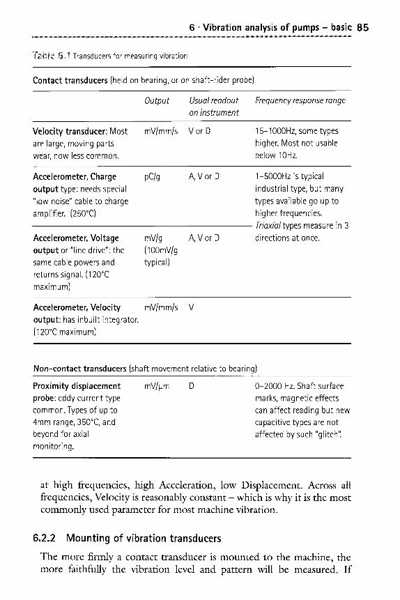
6 �9 Vibration analysis of pumps - basic 85
Tabte Go t Transducers for measuring vibration
Contact transducers (held on bearing, or on shaft-rider probe)
Output Usual readout on instrument
Frequency response range
Velocity transducer: Most are large, moving parts wear, now less common.
mV/mm/s Vor D 15- IO00Hz, some types higher. Most not usable below IOHz.
Accelerometer, Charge output type: needs special "low noise" cable to charge amplifier. (250~
pC/g A, Vor D
A, Vor D Aecelerometer, Voltage output or "line drive": the same cable powers and returns signal. (120~ maximum)
mV/g (lOOmV/g typical)
1-5000Hz is typical industrial type, but many types available go up to higher frequencies. Triaxial types measure in 3 directions at once.
Accelerometer, Velocity output: has inbuilt integrator. (120~ maximum)
mV/mm/s V
Non-contact transducers (shaft movement relative to bearing)
Proximity displacement probe: eddy current type common. Types of up to 4mm range, 350~ and beyond for axial monitoring.
mV/I.tm D 0-2000 Hz. Shaft surface marks, magnetic effects can affect reading but new capacitive types are not affected by such "glitch':
at high frequencies, high Acceleration, low Displacement. Across all frequencies, Velocity is reasonably constant- which is why it is the most commonly used parameter for most machine vibration.
6.2.2 Moun t i ng o f vibration transducers
The more firmly a contact transducer is mounted to the machine, the more faithfully the vibration level and pattern will be measured. If
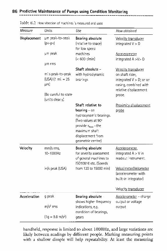
86 Predictive Maintenance of Pumps using Condition Monitoring
Table 6~ How vibration of machines is measured and used
Measure Units Use How obtained
Displacement pm peak-to-peak Bearing absolute Velocity transducer (pk-pk) (relative to space) integrated V > D
for low speed pm peak machines Accelerometer
(< 600 r/min) integrated A >V> D pm rms
mils peak-to-peak (USA) (I mil = 25 pm)
(Be careful to state (units clearly)
Shaft absolute- with hydrodynamic bearings
Shaft relative to bearing - on hydrodynamic bearings. (Two values at 900 provide Smax- the maximum shaft displacement from geometric centre)
Velocity transducer on shaft rider, integrated V > D; or on casing, combined with relative displacement probe.
Proximity displacement probe
Velocity mm/s rms, lO-lO00Hz
in/s peak (USA)
Bearing absolute for severity assessment of general machines to IS010816 etc. (Speeds from 120 to 15000 min)
Accelerometer, integrated A > V in readout instrument.
Ve Ioci meter/Ve Io meter (accelerometer with built-in integrator)
Velocity transducer
Acceleration g peak Bearing absolute- shows higher frequency
m/s 2 rms indications, e.g. condition of bearings,
(Ig = 9.8 m/s 2) gears
Accelerometer - charge output or voltage output
handheld, response is limited to about lO00Hz, and large variations are likely between readings by different people. Marking measuring points with a shallow dimple will help repeatability. At least the measuring
6 �9 Vibration analysis of pumps - basic 87
point should be marked. Acceptable results are however obtained with a handheld probe on rolling element bearings when measuring in the ultrasonic range, and above. A grease couplant may be needed.
Magnet mounting is convenient and on a flat surface can give faithful response up to about 2000Hz. High strength types are claimed to give up to perhaps 10 000Hz response. Types with two parallel feet hold well on less-than-flat surfaces. The holding force of the magnet will not be overcome below acceleration of 4g vertical or 2g horizontal mounting.
Studs, glued on or screwed in, are required for the best repeatability and highest frequency response. Some types use a quick-twist connector, requiring only one hand to mount
6.2.3 Point of measurement
For monitoring and evaluation of severity, machine vibration measure- ments with contact transducers are taken at the bearings, in three directions" Horizontal and Vertical usually in line with the shaft centreline, and Axial. For vertical shaft pumps, the two horizontal directions should be decided and clearly shown on a sketch: one in line with the suction pipe is usual, and others at flanges up to the top of the motor.
Routine monitoring of simple pumps may suffice with only some of these readings. For example, one radial reading at each bearing, usually horizontally, and one axial reading per shaft, requires much less time in collecting and processing than three readings per bearing. If used, triaxial accelerometers are usually mounted on top dead centre, and therefore will not measure horizontal nor axial vibration at the centreline.
On machines with hydrodynamic bearings, non-contact proximity displacement probes are sometimes installed permanently to sense shaft motion in X-Y directions at the bearings. For ease of access, they are usually placed at top dead centre + 45 ~ rather than at vertical and horizontal axes. These probes are however rarely fitted to pumps. Although temporary fitment using brackets or magnetic bases is possible, limited access to shafts minimize their use for investigations on pumps. From a diagnostic viewpoint, pump beating vibration measure- ments are considered to be more valuable than shaft measurements (Gopalakrishnan, 2000).
The outputs can be displayed on an oscilloscope or on a computer system via suitable software as displacement-time traces, or in XY mode, to give a shaft orbit, which is a magnified picture of the centreline
88 Predictive Maintenance of Pumps using Condition Monitoring
motion. The orbit will usually be elliptical, and changes shape if vibration of other frequencies is present. A flat orbit shows that a rotor is restrained unevenly. Orbits from shafts each side of a coupling can confirm alignment condition. If vibration at higher frequencies is present, it shows as ripples on the orbit. Processing instruments can filter out frequencies other than those at l x. More details about the use of shaft orbits and centreline motion can be found in Eisenmann and Eisenmann (1997) and through www.bently.com
Go3 Assessing the severity of vibration" general severity assessment
Whether the vibration of a machine is acceptable or not depends on the probability of damage to the machine itself, as well as its effects on the surroundings. Measurements should be taken when a machine is at its normal steady state operating conditions.
Vibration severity is usually expressed in:
�9 Displacement, for low speed machines at frequencies up to 10 Hz
�9 Velocity, for frequencies between 10-1000 H z - most machines fit here
�9 Acceleration, for frequencies above 1000 Hz.
To assess the allowable severity in any case, consider these points:
6.3.1 The effect on people and buildings
Steel flame buildings usually have natural frequencies below 10 H z - 40Hz, and may suffer cracks or other failure symptoms from excessive forced vibration levels. People experience discomfort at vibration frequencies below about 40 Hz.
6.3.2 The manufacturer's advice
The advice of manufacturers is likely to be conservative. Available Standards are often used (see below), as manufacturer's engineers are often involved in their formation.
6.3.3 Comparison with identical machines
Vibration measured identically on other 'identical' machines can be useful for comparison. However, such machines can have quite different vibration characteristics, yet all be in acceptable condition.
6 �9 Vibrat ion analysis of pumps - basic 8 9
6.3.4 General experience with machines
Several vibration severity guidelines are available, based on general experience with a range of machines. Engineering judgment is needed if there is any conflict between them. An apt comment in Eisenmann and Eisenmann (1997) sums up the situation: "There arc no universal vibration severity limits". The advice therefore is to choose the guidelines you feel carry the highest credibility and are the most appro- priate to your situation. Information is usually given with purchase of a vibration measurement instrument.
6.3.4.1 Bearing vibration Various national and international standards based on German experience in the 1960s have been current until recently superseded, but arc still useful. They are based on practical experience and give a useful set of criteria that can be used to assess machines in service, as well as for specifying vibration qualit 7 for new or overhauled machines.
As shown in Table 6.3, the criteria apply for machines with speeds between 600 and 12 000 r/rain, and give the maximum vibration level in any of horizontal, Vertical or Axial directions on the bearing caps, measured in line with the centre of the rotor. The unit is Velocity, m m / s rms. The assessment is broadband, with all vibration components between 10 to 1000 Hz included, each one being considered as of equal importance in severity.
Below 600 r /min, Displacement criteria are used. These criteria do not apply if a machine is affected by vibration transmitted from its surroundings to an extent of more than 1 /3 of its own service vibration. This can be checked with the machine shut down.
The shaded areas in Table 6.3 correspond to these gradings, from smoothest level downwards:
�9 A: GOOD to E X C E L L E N T - the smoothest expected from good manufacturing practice. New machines would normally fall here.
�9 B: SATISFACTORY- readily achieved by well-designed and well- made machines, and acceptable for long-term operation.
�9 C: NOT SATISFACTORY- higher than normally expected for well-made machines, possibly pointing to a fault. Unsuitable for continuous long-term operation. This level may be acceptable if the vibration is not due to machine deterioration.
�9 D: UNACCEPTABLE- there is unacceptably high probability of a severe fault or deterioration of the machine.
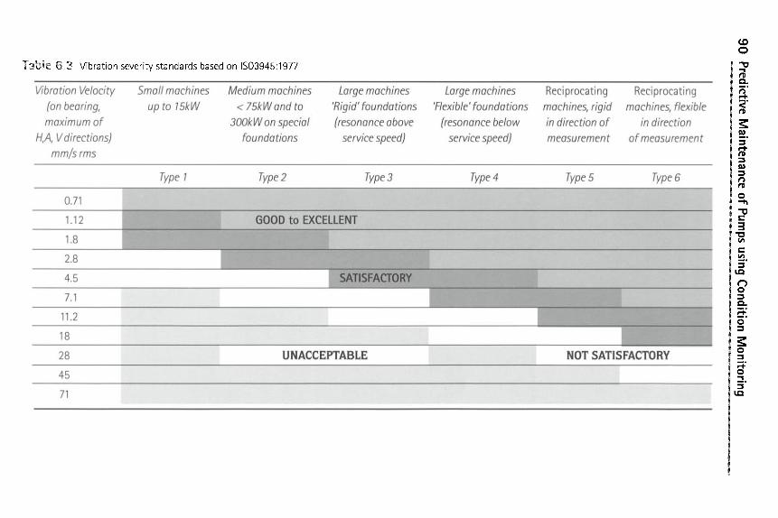
90 Predictive M
aintenance of Pumps using C
ondition Monitoring
r,~
03
LC)
*d-
03
C
~
c~ L
/3
c-
O
-o
~J
u3
co
_
O
L/3
co
-O
c-
(13
>.
r ~> r L/3
c-
O
.m
co
_O
LO
p~
6 �9 Vibration analysis of pumps - basic 91
To apply the table, it is necessary to decide if the machine has rigid or flexible supports. Rigidity is defined as when the combined machine and support structure has its lowest natural frequency in the direction of measurement at least 25% above its main excitation frequency (in most cases, the rotational frequency). All other support systems are ranked as flexible. A test may be needed if the class cannot be determined from drawings and calculation.
6.3.4.2 Shaft vibration levels Shaft vibration levels are greater than bearing vibration according to the relative stiffness of the structure and the bearing clearance. A practical limit is 50% of the bearing clearance, with shutdown at 70%. ISO 7919 provides guidelines for shaft vibration assessment for steam, gas and hydro turbosets, but not specifically for pumps. The basis is S m a x " the half amplitude of the orbit on its major axis.
A major pump manufacturer suggests that allowable peak-to-peak shaft displacement, unfiltered, for good performance should be 0.33 of bearing diametral clearance, with improvement desirable at up to 0.66, and correction required above 0.66 (Robinett and Kaiser, 2000).
6.3.4.3 Gearing and rolling element bearings Gearing and rolling element bearings are best monitored with higher frequency criteria. One such criterion is a casing vibration limit of 10 g peak for gear vibrations above 600 Hz. There are many specialist devices for assessing rolling element bearings, and the reader is referred to vendor information and the notes in Chapter 7.
6.3.5 Relating experience to required availability
An excellent example from experience with hundreds of process pumps at a large refinery showed that the minimum acceptable availability of 99.5% defined the maximum allowable vibration level of 5.6 m m / s rms. Availability reduced linearly to reach 98.5% at 13 m m / s (Hancock, 1974). Such development of a plant reliability model could well be more widely applied.
6.3.6 Consider actual experience with a particular pump
Where you have it, the best advice is from actual experience with the machine itself. As always, changes in vibration, particularly sudden ones, should be investigated.
6.3.6.1 Case study A pair of boiler feed pumps, each driven by a 7MW steam turbine, showed high vibration levels exceeding 17mm/s rms on the booster
92 Predictive Maintenance of Pumps using Condition Monitoring
pump beatings. Investigation showed that the vibration was transmitted from outside the booster pump, and therefore outside the criteria for use of the standard. These pumps have operated for many years without distress, despite the high levels. (The pumpset is shown in Figure 7.6, with the booster pump on the fight).
Where the expense is justified in critical cases, a thorough dynamic analysis could be made to find the actual forces present in the machine corresponding to the measured vibration levels, and then the stresses. A force, measured by use of a force hammer, is applied to the machine and the response is measured. These outputs are processed by an analyser and a specific computer program to find the frequency response functions, and sometimes also the operational deflection shapes. Finite element analysis can also be part of this process.
6~ Specific vibration severity standards for pumps
6.4.1 ISO 10816 Standards
ISO10816 Standards supersede ISO3945 mentioned above, and allow a wider frequency range to be agreed between parties. However, until guidelines for specific machines are developed and issued, the information in Table 6.3 applies. Several Parts have been released, each applying to particular machine types with more detailed criteria, e.g. ISO10816-3:1998 for centrifugal pumps. There are two criteria:
6.4.1.1 Overall vibration magnitude The philosophy is similar to the earlier ISO standards. Evaluation zones are given, defined as in A, B, C and D above. The values are not intended to be acceptance specifications, as these should be agreed between manufacturer and customer. They are intended to provide useful guidelines, and variations can be agreed. A synopsis is given in www.pruftechnikdirect, com/iso.html
As before, the pump must be classed as either rigid or flexible. Table 6.4 adapted from ISO10816-3:1998, applies for radial vibrations in the frequency range from 10 to 1000Hz. of all bearings, beating pedestals or housings under steady state operation at rated flow within the rated speed range. They do not apply during transients, and special allowance may be agreed for specific machines. Higher magnitudes can also be expected for some pumps, e.g. with special impellers, such as a non- clogging single vane type.
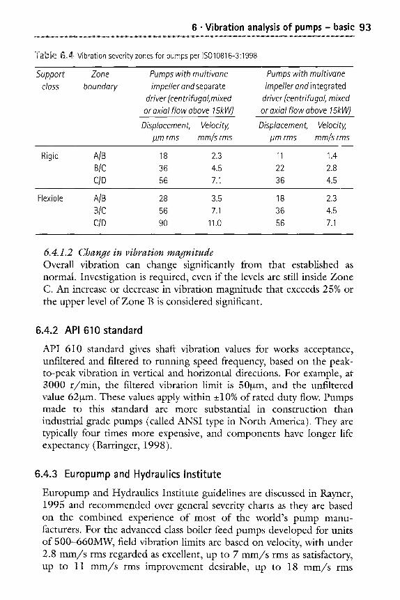
6 �9 Vibration analysis of pumps - basic 93
Table 6.4 Vibration severity zones for pumps per IS010816-3:1998
Support Zone Pumps with multivone class boundary impeller end separate
driver (centrifugal, mixed or axial flow above 15kW)
Displacement, Velocity, pm rms mm/5 rms
Pumps with multivane impeller and integrated
driver (centrifugal, mixed or axial flow above 15kW)
Displacement, Velocity, IJm rms mm/5 rms
Rigid A/B 18 2.3 11 1.4 B/C 36 4.5 22 2.8 C/D 56 7.1 36 4.5
Flexible A/B 28 3.5 18 2.3 B/C 56 7.1 36 4.5
C/D 90 11.0 56 7.1
6.4.1.2 Change in vibration magnitude Overall vibration can change significantly from that established as normal. Investigation is required, even if the levels are still inside Zone C. An increase or decrease in vibration magnitude that exceeds 25% or the upper level of Zone B is considered significant.
6.4.2 API 610 standard
API 610 standard ghTes shaft vibration values for works acceptance, unfiltered and filtered to running speed frequency, based on the peak- to-peak vibration in vertical and horizontal directions. For example, at 3000 r /min, the filtered vibration limit is 50~tm, and the unfiltered value 62~tm. These values apply within _+10% of rated duty flow. Pumps made to this standard are more substantial in construction than industrial grade pumps (called ANSI type in North America). They are typically four times more expensive, and components have longer life expectancy (Barringer, 1998).
6.4.3 Europump and Hydraulics Institute
Europump and Hydraulics Institute guidelines are discussed in Rayner, 1995 and recommended over general severity charts as they are based on the combined experience of most of the world's pump manu- facturers. For the advanced class boiler feed pumps developed for units of 500-660MW, field vibration limits are based on velocity, with under 2.8 m m / s rms regarded as excellent, up to 7 m m / s rms as satisfactory, up to 11 m m / s rms improvement desirable, up to 18 m m / s rms
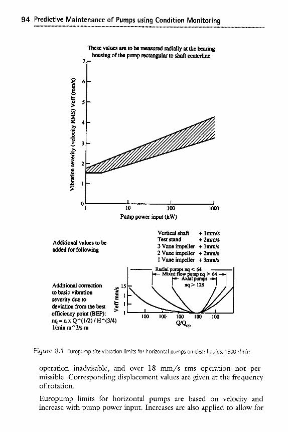
94 Predictive Maintenance of Pumps using Condition Monitoring
These values are to be measured radially at the bearing housing of the pump rectangular to shaft centerline
7 -
6
o 5 >,
r,/}
=: 4
> 3 v
,t. lt "5 8 2
.2
I
0 , 1
I . . . . I I lO lO0 lO00
Pump power input (kW)
Additional values to be added for following
Vertical shaft + lmm/s Test stand + 2mm/s 3 Vane impeller + lmm/s 2 Vane impeller + 2mm/s 1Vaneimpeller +3mm/s
Additional correction to basic vibration severity due to
deviation from the best efficiency point (BEP): nq - n x Q"(1/2) / H"(3/4) 1/min m"3/s m
Radial pumps nq < 64 _ Mix~.d flow pump nq > ~
^ ~ purn~ -'1 ! n q > 128 t
100 100 1t~ 100 1t~ Q/Q~
Figl.~re 6,t Europump site vibration limits for horizontal pumps on clear liquids. 1500 r/min
operation inadvisable, and over 18 m m / s rms operation not per- missible. Corresponding displacement values are given at the frequency of rotation.
Europump limits for horizontal pumps are based on velocity and increase with pump power input. Increases are also applied to allow for
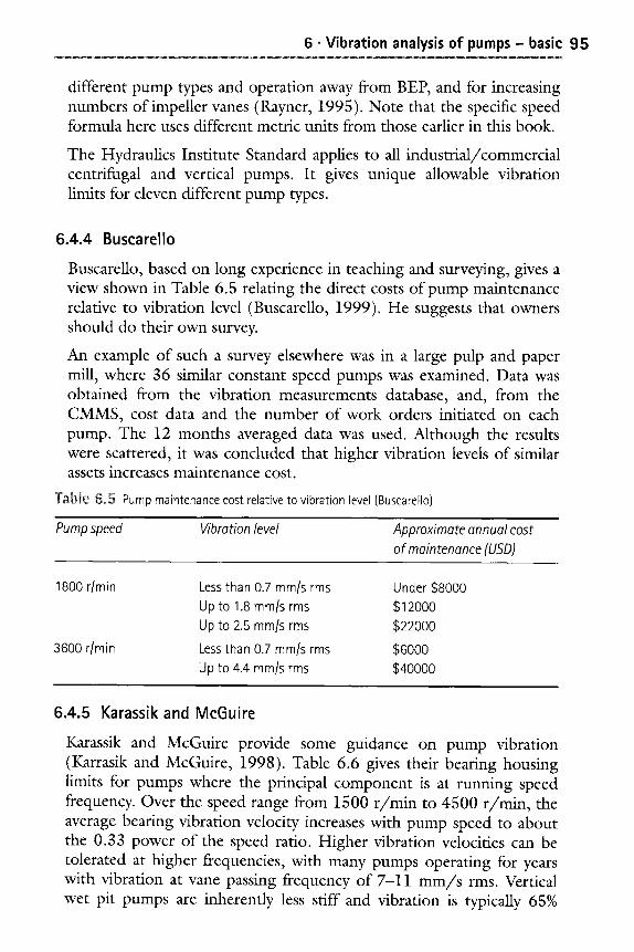
6 �9 Vibration analysis of pumps - basic 95
different pump types and operation away from B EP, and for increasing numbers of impeller vanes (Rayner, 1995). Note that the specific speed formula here uses different metric units from those earlier in this book.
The Hydraulics Institute Standard applies to all industrial/commercial centrifugal and vertical pumps. It gives unique allowable vibration limits for eleven different pump types.
6.4.4 Busearello
Buscarello, based on long experience in teaching and surveying, gives a view shown in Table 6.5 relating the direct costs of pump maintenance relative to vibration level (Buscarello, 1999). He suggests that owners should do their own survey.
An example of such a survey elsewhere was in a large pulp and paper mill, where 36 similar constant speed pumps was examined. Data was obtained from the vibration measurements database, and, from the CMMS, cost data and the number of work orders initiated on each pump. The 12 months averaged data was used. Although the results were scattered, it was concluded that higher vibration levels of similar assets increases maintenance cost.
TabJe 6~5 Pump maintenance cost relative to vibration level (Buscarello)
Pump speed Vibration level Approximate annual cost of maintenance (USD)
1800 r/min Less than 0.7 mm/s rms Under $8000 Up to 1.8 mm/s rms $12000 Up to 2.5 minis rms $22000
3600 r/min Less than 0.7 minis rms $6000 Up to 4.4 minis rms $40000
6.4.5 Karassik and McGuire
Karassik and McGuire provide some guidance on pump vibration (Karrasik and McGuire, 1998). Table 6.6 gives their bearing housing limits for pumps where the principal component is at running speed frequency. Over the speed range from 1500 r /min to 4500 r/min, the average bearing vibration velocity increases with pump speed to about the 0.33 power of the speed ratio. Higher vibration velocities can be tolerated at higher frequencies, with many pumps operating for years with vibration at vane passing frequency of 7-11 mm/s rms. Vertical wet pit pumps are inherently less stiff and vibration is typically 65%
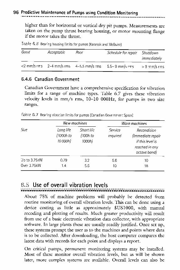
96 Predictive Maintenance of Pumps using Condition Monitoring
higher than for horizontal or vertical dry pit pumps. Measurements are taken on the pump thrust beating housing, or motor mounting flange if the motor takes the thrust.
Table 6o6 Bearing housing limits for pumps (Karassik and McGuire)
Good Acceptable Poor Schedule for repair Shutdown immediately
<2 mm/s rms 2-4 mm/s rms 4-5.5 mm/s rms 5.5- 9 mm/s rms > 9 mm/s rms
6.4.6 Canadian Government
Canadian Government have a comprehensive specification for vibration limits for a range of machine types. Table 6.7 gives these vibration velocity levels in m m / s rms, 10-10 000Hz, for pumps in two size ranges.
Tabie 6~ Bearing vibration limits for pumps (Canadian Government Specn)
Size
New machines
Long life Short life ( lO00h to ( 100h to lO000h) lO00h)
Worn machines
Service
required Recondition
(Immediate repair if this level is
reached in any octave band)
Up to 3.75kW 0.79 3.2 5.6 10 Over 3.75kW 1.4 5.6 10 18
.6.5 Use of overall vibration levels
About 75% of machine problems will probably be detected from routine monitoring of overall vibration levels. This can be done using a device costing as little as approximately $US1000, with manual recoding and plotting of results. Much greater productivity will result from use of a basic electronic vibration data collector, with appropriate software. In large plants these are usually readily justified. Once set up, these systems prompt the user as to the machines and points where data is to be collected. After downloading, the host computer compares the latest data with records for each point and displays a report.
On critical pumps, permanent monitoring systems may be installed. Most of these monitor overall vibration levels, but as will be shown later, more complex systems are available. Overall levels can also be
6 �9 Vibration analysis of pumps - basic 97
used for screening, to indicate the need investigation. See also Section 7.8 in this book.
for more advanced
Overall levels are sufficient when the problem is a "naturally" recurring one that cannot be designed out. An example is that of deposition on impeller vanes that builds up after varying periods in service and cannot be controlled on line. If vibration does not reduce after cleaning, then further investigation is needed.
6.5.1 Case study: Structural resonance
One of a pair of small end suction cooling water pumps (195L/s @ 107m) vibrated so severely that the discharge valve would wobble closed. The operators tied the valve open with rope! Investigation proved that the vibration level was indeed intolerable. The pump body provided all the support, with a large overhang to the coupling. A quick fix for high vibration that can be tried without much analysis, is to change the pump structure so that its resonance is moved away from rotation speed frequency.
The structure was stiffened temporarily with a jack, and much lower vibration resulted. Permanent stiffening brackets were welded to the base-plate, and bolted to the beating overhang on both sides, using the plugged holes that remained from the manufacturing process. This solution may not be the most elegant one, but may be sufficient and timely for the needs of the business. If no improvement results, then more refined investigation is needed, possibly leading to other solutions (see Chapter 7).
6.5.2 Case study: Misalignment
Misalignment is a common problem, and occurs in pumps when foundations settle unevenly. An increase in axial vibration is one indicator. In an admittedly unusual case, shims made of plain carbon steel were used instead of stainless steel. Water leakage caused rusting, sufficient to stretch the anchor bolts, alter alignment, and eventually break the bolts.
6.5.3 Case study: Structural looseness
Structural looseness in machine supports can be diagnosed by measuring overall vibration across interfacing parts. The measurements can be either vertical or horizontal. Except in severe cases, it is hard to detect structural looseness by touch. A common example is the anchor bolts holding down a bearing pedestal to its concrete foundation. These
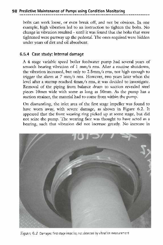
98 Predictive Maintenance of Pumps using Condition Monitoring ~ . ~ ~ ~ . ~ - > - . . . . . ~
bolts can work loose, or even break off, and not be obvious. In one example, high vibration led to an instruction to tighten the bolts. No change in vibration resul ted- until it was found that the bolts that were tightened were partway up the pedestal. The ones required were hidden under years of dirt and oil absorbent.
6.5.4 Case study: Internal damage
A 4 stage variable speed boiler feedwater pump had several years of smooth bearing vibration of 1 m m / s rms. After a routine shutdown, the vibration increased, but only to 2 .5mm/s rms, not high enough to trigger the alarm at 7 m m / s rms. However, two years later when the level after a startup reached 4 m m / s rms, it was decided to investigate. Removal of the piping from balance drum to suction revealed steel pieces 10mm wide with some as long as 50mm. As the pump has a suction strainer, the material had to come from within the pump.
On dismantling, the inlet area of the first stage impeller was found to have worn away, with severe damage, as shown in Figure 6.2. It appeared that the front wearing ring picked up at some stage, but did not seize the pump. The wearing face was thought to have acted as a bearing, such that vibration did not increase greatly. No increase in
o~z: Damaged first stage impeller, not detected by vibration measurement
6 �9 Vibration analysis of pumps - basic 9 9
motor current was observed. It had not been noticed that the pump speed had gradually ramped up to maintain the required flow, and performance condition monitoring had not been done.
References
API 610 (1995) Centrifugal pumps for refinery service 8th edition, American Petroleum Institute, Washington (9th Edition due 2003: Centrifugal pumps for the petroleum, petrochemical and natural gas industries) [Standard]
Barringer, HP (1998) Life cycle cost and good practices NPRA Maintenance Conference, San Antonio [Paper]
Buscarello, R (1999) Practical steps needed to change a company's machinery related culture RELIABILITY Vol 6, No 1, April, pp3-13 [Article]
Canadian Government Specification CDA/MS/NVSH 107 Vibration limits for maintenance [ Specification]
Eisenmann, RC (Sr) and Eisenmann, RC (1997) Machinery malfunction, diagnosis and correction Prentice Hall [Book].
Gopalakrishnan, S (2000) Software based diagnosis of feed pump problems Proceedings MARCON2000, Knoxville [Paper]
Guide to forecasting the vibrations of centrifugal pumps Europump May 1991
Hancock, WP (1974) How to control pump vibration Hydrocarbon Processing March, pp 107-113 [Article ]
Hydraulic Institute: Standards for centrifugal, rotary and reciprocating pumps ANSI/HI: 9.6.4 ISBN: 1-880952-45-9 [Standard]
ISO/FDIS 13373-1 (Draft in 2003) Condition monitoring and diagnostics of machines- Vibration condition monitoring- Part 1: General procedures [Standard]
ISO10816-1:1996 Evaluation of machine vibration by measurements on non- rotating parts - Part 1: General guidelines [Standard]
ISO10816-3:1998 Evaluation of machine vibration by measurements on non- rotating par ts - Part 3: Industrial machines with nominal power above 15k W and nominal speeds between 120 r/min and 15 000 r/min when measured in situ [Standard]
ISO7919-1:1996 Mechanical vibration of non-reciprocating mach ines - Measurements on rotating shafts sand evaluation criteria - Part 1: General guidelines [Standard]
Karassik, IJ and Grieve, T (1998) Centrifugal pumps Prentice-Hall [Book]
Rayner, R (1995) Pump Users Handbook, 4th Edition Elsevier [Book]

100 Predictive Maintenance of Pumps using Condition Monitoring
Robinett, FL and Kaiser, TF (2000) Vane pass vibration: source, assessment and
correction - a practical guide for centrifugal pumps: Part 2 RELIABILITY magazine, April [Paper]
www.bently.com [Website]
www.pruftechnikdirect, com/iso.html [Website]

Vibration analysis of pu m ps - adva need
methods
E Finding the vibration frequency i Using the vibration spectrum W Vibration phase angle .M Resonance M Rolling element bearings m Diagnosis of machine condition and faults @ Vertical pumps E Effect of internal wear on vibration m Control of vibration W Setting band levels for monitoring @ Permanent monitoring of pumps
7=1 Finding the vibration frequency
On other than very simple machines, vibration is often a combination of several frequency components of varying amplitudes. These must often be found for a more precise diagnosis of machine faults. This chapter will outline the methods available. A more thorough treatment can be found in the many books available in this topic. Some are listed in the bibliography. Goldman, 1999 is a good starting point, and www.iLearnInteractive.com is recommended for training in this field.
An vibration amplitude-time trace (i.e. in the time domain) viewed on an oscilloscope will usually show that one or more frequencies are present in addition to the basic signal, which is usually at the frequency corresponding to running speed. A better method is to use a frequency analyser to see the vibration pattern in the frequency d o m a i n - called the vibration spectrum, or vibration signature as it will be unique to
102 Predictive Maintenance of Pumps using Condition Monitoring
that machine at that point of measurement. The results of various exciting forces inside a machine are shown in its vibration spectrum, providing a "window" into the machine, and any change in the signature indicates a change in the machine. Whether this is significant in assessing machine health is a matter of training and experience.
Signature analysis is much more sensitive to changes in machine condition than overall measurement alone. A large change in one vibration component could indicate a significant change in the machine, yet result in little change in the overall vibration level.
The simplest and oldest type of analyser is manually tuned like a radio, and displays the amplitude at each tuned frequency on a meter. The spectrum display is obtained by tuning the filter slowly through the frequency range of interest and plotting the maximum amplitude readings found at each frequency, either manually or using a chart recorder.
7.1.1 Filters and scaling
Most manual analysers have constant percentage bandwidth filters, with 3% and 10% being common. 1 /3 Octave analysers are commonly used in analysis of noise, and correspond to 23% bandwidth. The resolution of the filter governs how sharply it cuts off other signals each side of the tuned frequency. A logarithmic frequency scale is usual with these filters.
Linear amplitude scaling is best for diagnosis and reporting, as the relative vibration components can be judged by eye. Logarithmic scaling is better for monitoring, as it reveals minor components more clearly, that may be important indicators of a change in machine condition.
Some manual analysers have an output for triggering a stroboscope, used for phase measurement for further diagnosis and field balancing.
The frequency scale can be expressed in Hz or CPM, and is sometimes given in orders of rotation speed. This shows more clearly the frequency components that are multiples of rotation frequency, or synchronous. We shall call this rotation speed component Ix, but it is also known as 1st Order, 1/rev, fundamental, or the 1st Harmonic (note that the terminology used in music differs, and musicians would call this the 2nd Harmonic!).
The signature up to 1000Hz from the vibration on a bearing of a multistage boiler feed pump is shown in Figure 7.1, and was obtained with a manual analyser with constant percentage bandwidth filters. The
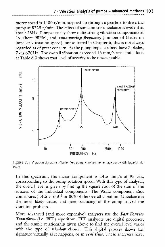
7 �9 Vibration analysis of pumps - advanced methods 1 0 3
motor speed is 1480 r /min, stepped up through a gearbox to drive the pump at 5728 r /min. The effect of some motor unbalance is evident at about 25Hz. Pumps usually show quite strong vibration components at lx, (here 95Hz), and vane-passing frequency (number of blades on impeller x rotation speed), but as stated in Chapter 6, this is not always regarded as of great concern. As the pump impellers here have 7 blades, 7x is 670Hz. The overall vibration exceeded 16 m m / s rms, and a look at Table 6.3 shows that level of severity to be unacceptable.
I0
5
I 7 95 25
PUMP SPEED
VANE PASSING FREQUENCY E
E >.- t.-- L.J 0 __1 u.t
Z C:) I--- < Q::
I I I
10 50 100 FREQUENCY Hz
I . . . . . I
500 1000
Figur'e 7,1 Vibration signature of boiler feed pump: constant percentage bandwidth, logarithmic
scales
In this spectrum, the major component is 14.5 m m / s at 95 Hz, corresponding to the pump rotation speed. With this type of analyser, the overall level is given by finding the square root of the sum of the squares of the individual components. The 95Hz component thus contributes [ 14.5 + 16.3 ]2 or 80% of the overall vibration. Unbalance is the most likely cause, and here balancing of the pump solved the vibration problem.
More advanced (and more expensive) analysers use the Fast Fourier Transform (i.e. FFT) algorithm. FFT analysers use digital processes, and the simple relationship given above to find the overall level varies with the type of window chosen. This digital process shows the signature virtually as it happens, or in real time. These analysers have,
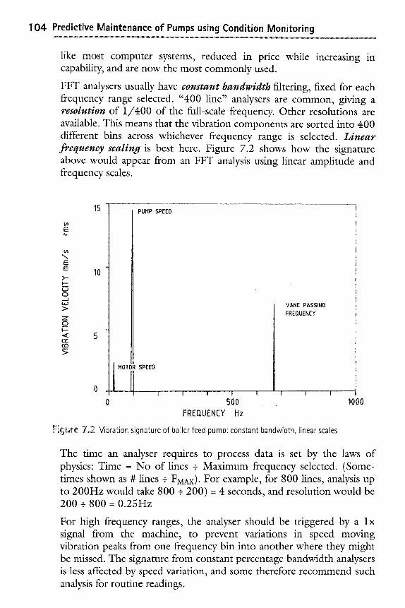
104 Predictive Maintenance of Pumps using Condition Monitoring
like most computer systems, reduced in price while increasing in capability, and are now the most commonly used.
FFT analysers usually have constant bandwidth filtering, fixed for each frequency range selected. "400 line" analysers are common, giving a resolution of 1 /400 of the full-scale frequency. Other resolutions are available. This means that the vibration components are sorted into 400 different bins across whichever frequency range is selected. Linear frequency scaling is best here. Figure 7.2 shows how the signature above would appear from an FFT analysis using linear amplitude and frequency scales.
15
"x
E E 10
o - . J
z o t-- ~ 5 en
MOTOR SPEED
Jl L 0
PUMP SPEED
I ..... I I I '' I
500
FREQUENCY Hz
VANE PASSING FREQUENCY
I t I
Figure 7~ Vibration signature of boiler feed pump constant bandwidth, linear scales
10(
The time an analyser requires to process data is set by the laws of physics: Time = No of lines + Maximum frequency selected. (Some- times shown as # lines + F~.x). For example, for 800 lines, analysis up to 200Hz would take 800 + 200) = 4 seconds, and resolution would be 200 + 800 = 0.25Hz
For high frequency ranges, the analyser should be triggered by a l x signal from the machine, to prevent variations in speed moving vibration peaks from one frequency bin into another where they might be missed. The signature from constant percentage bandwidth analysers is less affected by speed variation, and some therefore recommend such analysis for routine readings.
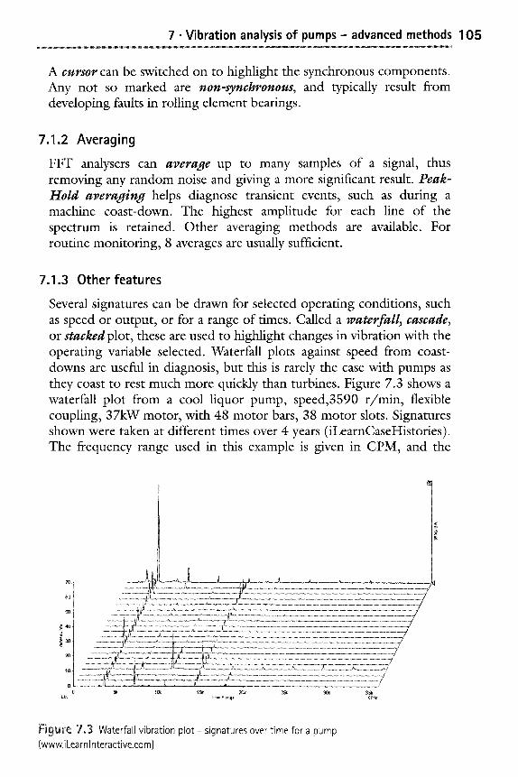
7 �9 Vibration analysis of pumps - advanced methods 1 0 5
A cursor can be switched on to highlight the synchronous components. Any not so marked are non-synchronous, and typically result from developing faults in rolling element bearings.
7.1.2 Averaging
FFT analysers can average up to many samples of a signal, thus removing any random noise and giving a more significant result. Peak- Hold averaging helps diagnose transient events, such as during a machine coast-down. The highest amplitude for each line of the spectrum is retained. Other averaging methods are available. For routine monitoring, 8 averages are usually sufficient.
7.1.3 Other features
Several signatures can be drawn for selected operating conditions, such as speed or output, or for a range of times. Called a waterfall, cascade, or stacked plot, these are used to highlight changes in vibration with the operating variable selected. Waterfall plots against speed from coast- downs are useful in diagnosis, but this is rarely the case with pumps as they coast to rest much more quickly than turbines. Figure 7.3 shows a waterfall plot from a cool liquor pump, speed,3590 r /min , flexible coupling, 37kW motor, with 48 motor bars, 38 motor slots. Signatures shown were taken at different times over 4 years (iLearnCaseHistories). The frequency range used in this example is given in CPM, and the
............ ~ ....................................................... {~" . . . . . . . . . . . . . . . . . . . . . . . . . . . . . . . . . . . . . . . . . . . . . . . . . . . 7.: . . . . . . . . . . . . . . . . . . . . . . . . . . . . . . . . . . . . . . . . . . . . . .,,t, . . . . . . . . . . . . . .
.,{ /
,, ..:"s ' ~ : ~ .................................. "":~ .............. :L.~:~ ................................................................. /
. . . . . . . . . . . . . . . . . . . & . . . . . . . . . L . . . . . . . . . . . . . . . . . . . . . . . . . . . . . . . . . . . . . .~ . . . . . . . . . . . . . . . . .
. . . . . . . . . . . . ~ :CC~;""2;F" ~ . . . . . . . . . . . . . . . . . . . . . . . . . . . . . . " 7 -
"1 ==================================== .... i~J' ......... / ..................... -~ ................ ~"+ .................... il ............. ::C:::,~I:. ...,,, ................................... /
o. -~
o ~ -~ok 1~ ~ 2~ ~ ~4~
Figure 7.3 Water fa l l v ib ra t ion p lot - s ignatures over t ime for a pump
(www. i Lea rnln tera ct ive.co m)
106 Predictive Maintenance of Pumps using Condition Monitoring ~ ~ , ~ . - ~ - , ~ ~ . . . . . . . . . . .
latest signature shows a rapid increase in the l x component. A strong component at 4x is the vane passing rate.
It is often convenient to tape record the raw vibration, and analyse in various ways later. FM tape recorders using video-type cassettes are convenient and give high performance. Some special vibration instruments are capable of recording such dynamic data, usually in conjunction with a computer, and enhancement of such capability will surely continue.
Electronic data collector/analysers are available for field use from several manufacturers. The vibration signature shows on a LCD screen. More advanced features are continually appearing in these systems, and a recent type adapts a PDA to give a very compact device. Date is taken on bearings according to a route set up by the user, with the help of special software. The recorded data is transferred into the computer and compared with the signatures from past samples. Differences can be seen manually, or with alert and alarm levels of amplitude set in frequency bands selected by the user. Decision support systems are available to automate this process, and can be expected to increase in reliability and capability. Some systems have coded mounting points so that the details of the point are automatically registered when the transducer is attached, thus eliminating errors.
The frequency range, or ranges, to be used are selected accordingly, as is the parameter to be used for vibration amplitude. Mathematically, Displacement accentuates the lower frequencies, Acceleration the higher, and Velocity the mid-range. For most routine pump work, velocity up to 1000Hz is sufficient, but acceleration can be useful in highlighting rolling element bearing condition.
Dual and multi-channel analysers provide enhanced capability, such as cross-correlation and coherence, and are mostly used by specialists. The ability to zoom in on a selected range of frequency is useful to increase the resolution for better diagnosis.
7,2 Using the vibration spectrum
Knowledge of the vibration frequency components provides more insights into the cause of vibration. For example:
unbalance gives vibration at l x 3x).
, sometimes with harmonics (2x,
misalignment also gives vibration at lx , but usually 2x is dominant. Higher axial vibration is also an indicator of misalignment. The effects of misalignment are similar to those from unbalance.
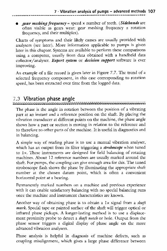
7 �9 Vibration analysis of pumps - advanced methods 1 0 7
gear meshing frequency = speed x number of teeth. (Sidebands are often visible as gears wear: gear meshing frequency _+ rotation frequency, and their multiples).
Charts of symptoms and their likely causes are usually provided with analysers (see later). More information applicable to pumps is given later in this chapter. Systems are available to perform these comparisons using a computer, usually from data obtained with a handheld data collector/analyser. Expert system or decision support software is ever improving.
An example of a file record is given later in Figure 7.7. The trend of a selected frequency component, in this case corresponding to rotation speed, has been extracted over time from the logged data.
7~ Vibration phase angle
The phase is the angle in rotation between the position of a vibrating part at an instant and a reference position on the shaft. By placing the vibration transducer at different points on the machine, the phase angle shows how a part or section is moving in relation to the reference and to therefore to other parts of the machine. It is useful in diagnostics and in balancing.
A simple way of reading phase is to use a manual vibration analyser, which has an output from its filter triggering a stroboscope when tuned to l x. These instruments are designed for field balancing of rotating machines. About 12 reference numbers are usually marked around the shaft. For pumps, the coupling can give enough area for this. The tuned stroboscope flash shows the phase by illuminating the appropriate shaft number at the chosen datum point, which is often a convenient horizontal point at a bearing.
Permanently marked numbers on a machine and previous experience with it can enable satisfactory balancing with no special balancing runs once the machine and instrument characteristics are known.
Another way of obtaining phase is to obtain a l x signal from a shaft mark. Special tape or painted surface of the shaft will trigger optical or infrared phase pickups. A longer-lasting method is to use a displace- ment proximity probe to detect a shaft notch or hole. Output from the phase sensor triggers a digital display of phase angle on the more advanced vibration analysers.
Phase analysis is helpful in diagnosis of machine defects, such as coupling misalignment, which gives a large phase difference between
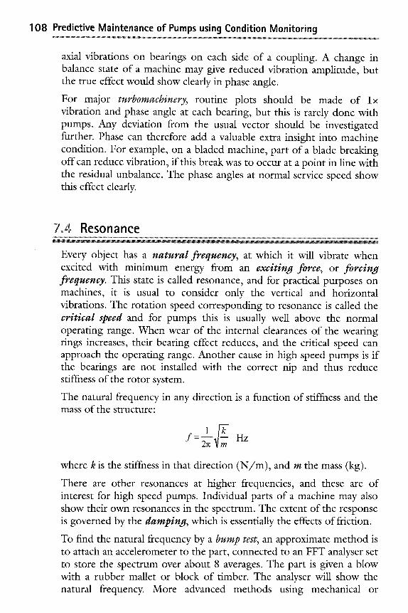
108 Predictive Maintenance of Pumps using Condition Monitoring
axial vibrations on bearings on each side of a coupling. A change in balance state of a machine may give reduced vibration amplitude, but the true effect would show clearly in phase angle.
For major turbomachinery, routine plots should be made of l x vibration and phase angle at each bearing, but this is rarely done with pumps. Any deviation from the usual vector should be investigated further. Phase can therefore add a valuable extra insight into machine condition. For example, on a bladed machine, part of a blade breaking off can reduce vibration, if this break was to occur at a point in line with the residual unbalance. The phase angles at normal service speed show this effect clearly.
7~ Resonance
Every object has a natural frequency, at which it will vibrate when excited with minimum energy from an exciting force, or forcing frequency. This state is called resonance, and for practical purposes on machines, it is usual to consider only the vertical and horizontal vibrations. The rotation speed corresponding to resonance is called the critical speed and for pumps this is usually well above the normal operating range. When wear of the internal clearances of the wearing rings increases, their bearing effect reduces, and the critical speed can approach the operating range. Another cause in high speed pumps is if the bearings are not installed with the correct nip and thus reduce stiffness of the rotor system.
The natural frequency in any direction is a function of stiffness and the mass of the structure:
Hz
where k is the stiffness in that direction (N /m) , and m the mass (kg).
There are other resonances at higher frequencies, and these are of interest for high speed pumps. Individual parts of a machine may also show their own resonances in the spectrum. The extent of the response is governed by the damping, which is essentially the effects of friction.
To find the natural frequency by a bump test, an approximate method is to attach an accelerometer to the part, connected to an FFT analyser set to store the spectrum over about 8 averages. The part is given a blow with a rubber mallet or block of timber. The analyser will show the natural frequency. More advanced methods using mechanical or
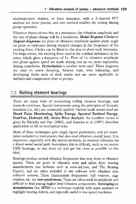
7 �9 Vibration analysis of pumps - advanced methods 1 0 9
electrodynamic shakers, or force hammers, with a 2-channel FFT analyser are more precise, and one method enables the testing during pump operation.
Vibration theory shows that at a resonance, the vibration amplitude and the rate of phase change will be a maximum. Modal Response Circles or Nyquist diagrams are plots of vibration amplitude against phase angle on polar co-ordinates during stepped changes in the frequency of the exciting force. Circles can be fitted to the data to show each resonance. For large rotors, the exciting force used is the residual unbalance in the rotor, which gives a frequency of l x. Plots of l x vibration amplitude and phase against speed are made during run-up or, more repeatably, during coastdown. Perturbation is another term used. These diagrams are used to assess damping, balance state, trim balancing, and developing faults such as shaft cracks and are more applicable to turbines and compressors than to pumps.
7.5 Rolling element bearings
There are many ways of monitoring rolling element bearings, and research continues. Special instruments using the principles of Acoustic Emission (i.e. AE) are commonly applied. Various trade names used are Shock Pulse Monitoring, Spike Energy, Spectral Emitted Energy, PeakVue, Hol royd AE, Stress Wave Analysis. An excellent review is given by Sikorska and Pan (2003), and Kataoka et al (1987) describes application of AE to mechanical seals.
Most of these techniques give single figure parameters, and are some- times included in instruments that also read vibration overall level. It is important, especially with the special methods, to measure vibration via a direct metal-metal path. Sometimes this is difficult, such as on motor NDE bearings, so one must try and get the close as possible to this ideal.
Bearings produce several vibration frequencies that may show in vibration spectra. These are given in vibration texts and tables from bearing manufacturers (see websites such as www.skf.com, and The Bearing Expert), and are often included in the software with vibration data collector systems. These characteristic frequencies" ball rotation, cage rotation, etc. are non-synchronous. These are often small in amplitude and difficult to find among higher level vibration components. Enveloping or demodulation (i.e. HFD) is a technique available with some analysers to highlight bearing defects, and especially useful in low speed machines.
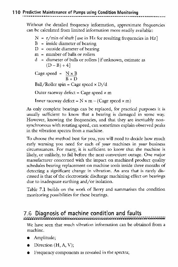
1 10 Predictive Maintenance of Pumps using Condition Monitoring
Without the detailed frequency information, approximate frequencies can be calculated from limited information more readily available:
N = r / m i n of shaft [use in Hz for resulting frequencies in Hz] B = inside diameter of bearing D = outside diameter of bearing m = number of balls or rollers d = diameter of balls or rollers [if unknown, estimate as
( D - B ) +4]
Cage speed = N x B B + D
Ball/Roller spin = Cage speed x D / d
Outer raceway defect = Cage speed x m
Inner raceway defect = N x m - (Cage speed x m)
As only complete bearings can be replaced, for practical purposes it is usually sufficient to know that a beating is damaged in some way. However, knowing the frequencies, and that they are inevitably non- synchronous with rotating speed, can sometimes explain observed peaks in the vibration spectra from a machine.
To choose the method best for you, you will need to decide how much early warning you need for each of your machines in your business circumstances. For many, it is sufficient to know that the machine is likely, or unlikely, to fail before the next convenient outage. One major manufacturer concerned with the impact on machined product quality schedules bearing replacement on machine tools inside three months of detecting a significant change in vibration. An area that is rarely dis- cussed is that of the electrostatic discharge machining effect on bearings due to inadequate earthing and /o r isolation.
Table 7.1 builds on the work of Berry and summarises the condition monitoring possibilities for these bearings.
7~ Diagnosis of machine condition and faults
We have seen that much vibration information can be obtained from a machine.
�9 Amplitude;
�9 Direction (H, A, V);
�9 Frequency components as revealed in the spectra;

7 �9 Vibration analysis of pumps - advanced methods 1 1 1
Table 7.1 Rolling element bearings - stages of degradation and condition monitoring
Stage of bearing Noise level Temperature wear
Vibration - overall, Crest Factor, frequency analysis,
demodulation
Vibration - acoustic emission methods- SPM, SE SEE, HF-AE
etc.
Stage I - Normal Normal Normal Noticeable increase (BUT: other sources too- pump cavitation, high speed gears, gas leaks)
Stage 2 -less than 20% bearing life left
Slight change
Normal Slight increase in Acceleration. Resonances of bearing components show. At end of this Stage, sidebands
appear on these reso n a n ces
Large increase
Stage 3 -less than 5% bearing life left
Audible to Slight a trained increase ear, but (not on repeatability recirculating is poor oil systems)
Large increase in Acceleration and Velocity.
Bearing defect frequencies and harmonics are now detectable and growing, also sidebands are evident on these and also on component resonances.
Very high levels
Stage 4 - about Change in Significant 1Olo of bearing pitch clearly increase life left audible
Significant increase Gradual decline, in Displacement then rapid increase and Velocity, I/rev to very high levels. and harmonics show. High "noise floor"
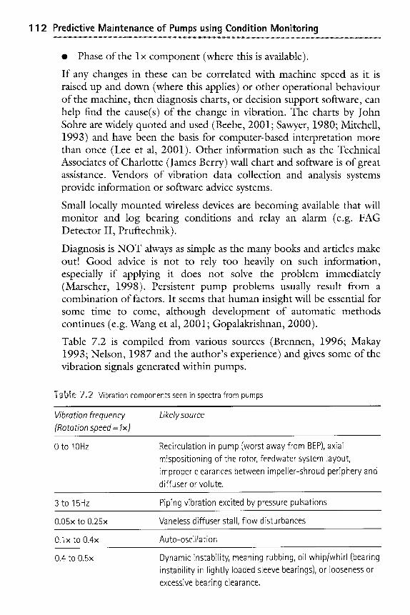
1 12 Predictive Maintenance of Pumps using Condition Monitoring
�9 Phase of the l x component (where this is available).
If any changes in these can be correlated with machine speed as it is raised up and down (where this applies) or other operational behaviour of the machine, then diagnosis charts, or decision support software, can help find the cause(s) of the change in vibration. The charts by John Sohre are widely quoted and used (Beebe, 2001; Sawyer, 1980; Mitchell, 1993) and have been the basis for computer-based interpretation more than once (Lee et al, 2001). Other information such as the Technical Associates of Charlotte (James Berry) wall chart and software is of great assistance. Vendors of vibration data collection and analysis systems provide information or software advice systems.
Small locally mounted wireless devices are becoming available that will monitor and log beating conditions and relay an alarm (e.g. FAG Detector II, Pruftechnik).
Diagnosis is NOT always as simple as the many books and articles make out! Good advice is not to rely too heavily on such information, especially if applying it does not solve the problem immediately (Marscher, 1998). Persistent pump problems usually result from a combination of factors. It seems that human insight will be essential for some time to come, although development of automatic methods continues (e.g. Wang et al, 2001; Gopalakrishnan, 2000).
Table 7.2 is compiled from various sources (Brennen, 1996; Makay 1993; Nelson, 1987 and the author's experience) and gives some of the vibration signals generated within pumps.
T~bie 7...2 Vibration components seen in spectra from pumps
ViOration frequency [Rotation speed = lx)
Likelysource
0 to lOHz Recirculation in pump (worst away from BEP), axial mispositioning of the rotor, feedwater system layout, improper clearances between impeller-shroud periphery and diffuser or volute.
3 to 15Hz Piping vibration excited by pressure pulsations
O.05x to 0.25x Vaneless diffuser stall, flow disturbances
O. 1 x to 0.4x Auto-oscillation
0.4 to 0.5x Dynamic instability, meaning rubbing, oil whip/whirl (bearing instability in lightly loaded sleeve bearings), or looseness or excessive bearing clearance.
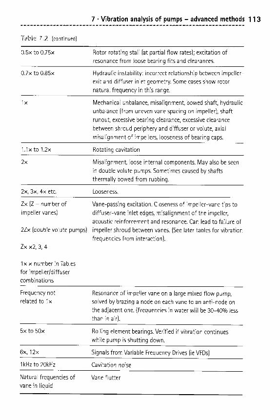
7 �9 Vibration analysis of pumps - advanced methods 1 13
Table 7.2 (continued)
O.5x to 0.75x Rotor rotating stall (at partial flow rates); excitation of resonance from loose bearing fits and clearances.
0.7x to 0.85x Hydraulic instability: incorrect relationship between impeller- exit and diffuser inlet geometry. Some cases show rotor natural frequency in this range.
lx Mechanical unbalance, misalignment, bowed shaft, hydraulic unbalance (from uneven vane spacing on impeller), shaft runout, excessive bearing clearance, excessive clearance between shroud periphery and diffuser or volute, axial misalignment of impellers, looseness of bearing caps.
1.1x to 1.2x Rotating cavitation
2x Misalignment, loose internal components. May also be seen in double volute pumps. Sometimes caused by shafts thermally bowed from rubbing.
2x, 3x, 4x etc. Looseness.
Zx (Z = number of Vane-passing excitation. Closeness of impeller-vane tips to impeller vanes) diffuser-vane inlet edges, misalignment of the impeller,
acoustic reinforcement and resonance. Can lead to failure of 2Zx (double volute pumps) impeller shroud between vanes. (See later tables for vibration
frequencies from interaction). Zx x2, 3, 4
l x x number in Tables for impeller/diffuser combinations
Frequency not related to lx
Resonance of impeller vane on a large mixed flow pump, solved by brazing a node on each vane to an anti-node on the adjacent one. (Frequencies in water will be 30-40% less than in air).
5x to 50x Rolling element bearings. Verified if vibration continues while pump is shutting down.
6x, 12x Signals from Variable Frequency Drives (ie VFDs)
1 kHz to 20kHz Cavitation noise
Natural frequencies of vane in liquid
Vane flutter

114 Predictive Maintenance of Pumps using Condition Monitoring
7.6.1 Mechanical unbalance
Mechanical unbalance of the impeller can result from uneven wear / erosion, corrosion, deposits distributed unevenly on blades or shrouds, from foreign objects caught in the impeller, impeller not balanced correctly, or parts not fitted properly. A recent bulletin board case reported finding a piece of steel 50mm diameter, 16mm thick jammed in an impeller. In another case, on a 2-stage double suction slow speed pump, a piece of lead weighing 1.5kg was found nailed and wired inside the cavity of one of the impellers, in a practical attempt at balancing. Figure 7.4 shows a dramatic cause of unbalance. Another impeller in the pump had part of the inlet section of a vane missing.
Figure 7...4 Impeller with severe shroud damage
Balancing is a common way to reduce l x vibration, even if only temporarily, and should be cost-effective to achieve acceptable vibration levels to suit the needs of the business (this is not necessarily "perfect" balance). Table 7.2 gives some balancing methods applicable to pumps. Available Standards (Ref ISO, API) can be used as a guide. ISO Grade G6.3 is given for pump impellers, meaning that the residual specific unbalance ( g . m m / k g ) x rotation velocity (rad/s) is 6.3 for correction in one plane.
7 �9 Vibrat ion analysis of pumps - advanced methods 1 1 5
For example, the service speed of an impeller of mass 5 kg is 3000r/min, or 50Hz. Its permissible residual specific unbalance for Grade 6.3 is therefore"
6 . 3 x 1000
50 • 2~: - 2 0 g . m m / k g
The unbalance for this impeller is therefore 100 g.mm. If the impeller is to be balanced in two planes, this would be 50 g.mm per plane. The API610 recommendation is 6350W/N, where W is the mass of the impeller at a journal (kg) and N its maximum operating speed (r/min). ( 4 W / N using pounds and r/min).
ISO Grade 6.3 is supported for single-stage pumps (Nevlik and Jackson, 1995). Some practitioners favour precision balancing to ISO Grade G1, stretching to G2.5 (Buscarello), while others consider this is too fight and beyond the capability of most industrial balancing machines.
7.6.1.1 The timed oscillation method for single-plane balancing This method has been used successfully for short rotors such as pump impellers on mandrels (using a pot magnet as the swing weight), and also in situ for overhung fans up to 2m diameter with rolling element bearings. The impeller must be set up on a mandrel, and it is desirable to fill the keyway temporarily.
The method was developed and used for a 10-stage pump (2970 r /min) of the ring-section design, where each impeller is assembled in turn with its matching stationary diffuser section. Balancing of the individual impellers is more likely to result in smooth vibration than balancing of the assembly as a whole, where the corrections are only made on the end impellers.
Parallel ways were clamped to the bed of a milling machine. The correction was made on the adjacent machine using an end-milling cutter. A table was calculated and drawn up giving the depth of cut required in each case. The position was marked clearly on the impeller, and it was passed to the machinist who cut the required mass from the back shroud.
The source of the method is not known, but is believed to derived from the theory of the compound pendulum. Here is the procedure"
Mark numbers around the impeller, evenly spaced. Marking in line with the blades is usual.
Choose a swing weight to fasten (by clamp or magnet) on the impeller, to give to-and-fro oscillation time of about 20 seconds.
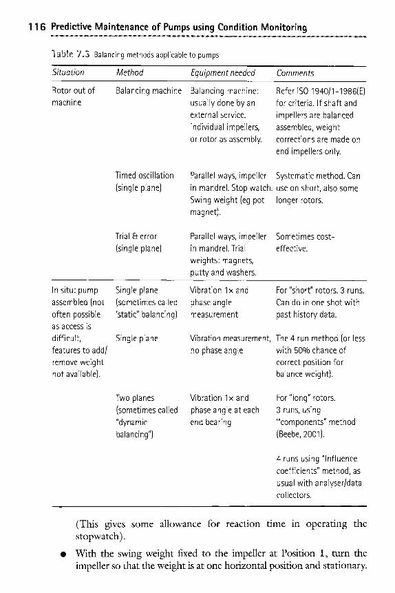
1 1 6 Predictive Maintenance of Pumps using Condition Monitoring
Table 7.3 Balancing methods applicable to pumps
Situation Method Equipment needed Comments
Rotor out of Balancing machine machine
Timed oscillation (single plane)
Trial & error (single plane)
Balancing machine: usually done by an external service. Individual impellers, or rotor as assembly.
Refer ISO 1940/1-1986(E) for criteria. If shaft and impellers are balanced assembled, weight corrections are made on end impellers only.
Parallel ways, impeller Systematic method. Can in mandrel. Stop watch, use on short, also some Swing weight (eg pot longer rotors. magnet).
Parallel ways, impeller in mandrel. Trial weights: magnets, putty and washers.
Sometimes cost- effective.
In situ: pump assembled {not often possible as access is difficult, features to add/ remove weight not available).
Single plane (sometimes called 'static" balancing)
Single plane
Two planes (sometimes called "dynamic balancing")
Vibration lx and phase angle measurement
For "short" rotors. 3 runs. Can do in one shot with past history data.
Vibration measurement, The 4 run method (or less no phase angle with 50% chance of
correct position for balance weight}.
Vibration lx and phase angle at each end bearing
For "long" rotors. 3 runs, using '"components" method {Beebe, 2001).
4 runs using "Influence coefficients" method, as usual with analyser/data collectors.
(This gives some allowance for reaction time in operating the stopwatch).
With the swing weight fixed to the impeller at Position 1, turn the impeller so that the weight is at one horizontal position and stationary.
7 �9 Vibration analysis of pumps - advanced methods 1 17
�9 Release the weight and let the impeller swing freely under its own inertia - do not push it in any way.
�9 Time the to-and-fro oscillation from the horizontal position.
�9 Turn the impeller so that the weight is at the horizontal position on the other side, and repeat.
�9 Take the average time of swing for this position, and plot on a graph of time vs position (with position numbers evenly spaced: position 1 appears twice- at the start and the end of the position axis).
�9 Move swing weight to Position 2, etc. and repeat process in turn for each position around the impeller.
�9 Connect the graphed points with a smooth sine wave shape line, and read off the maximum and minimum times of swing- Tand t.
�9 Calculate the size of balance weight required from"
T 2 _ t 2 Balance weight- Swing weight x T 2 + l 2
Make a balance weight of the required mass, and make the correction by removing mass from the impeller rear shroud at the position of m i n i m u m swing. On large impellers, it may be possible to fix a weight on to the impeller such that it does not interfere with liquid flow, and in this case, the position is in line with the m a x i m u m swing time. The fixing must of course be sufficiently strong not to allow the mass to fly off at operating speed. If welded, allow for the mass of the weld.
Check the result if desired by repeating the swing test for 3 spaced points around the impeller.
7.6.2 Hydraulic unbalance
Hydraulic unbalance results when the pulses of liquid are not even, and the force they produce is also not even. A mystery lx vibration on some large boiler fcedwater pumps, despite mechanical balancing of the impellers, was found to be due to use of non-OEM impellers with outlet widths varying up to 10%. This resulted in non-uniform liquid flow passages and forces, giving the same symptom as mechanical unbalance. The only cure is higher quality castings with the outlet widths within 1%. The same can be expected from uneven spacing of the vanes. Laboratory experiment has confirmed that the amplitude of the force varies with the deviation in passage size, and the amplitude and phase vary with the flow rate (u 1998).
1 1 8 Predictive Maintenance of Pumps using Condition Monitoring
7.6.3 Misalignment
Misalignment between the pump and its driver is a major cause of vibration, and usually results in a high axial vibration of up to 1.5 times the radial level. Some claim that higher misalignment results in increased energy consumption, but this has not been found in carefully run tests (Hines et al 1997). High misalignment can however be expected to increase bearing loads and shorten their life (Jesse et al, 1999; Hines et al, 1999).
The frequency of vibration is usually at running speed or twice and other multiples (Nelson, 1987). Causes can be loose foundation bolts, flexible baseplate, piping loads, bearing degradation, incorrect axial setting for flexible coupling, and incorrect allowance for thermal growth (expansion of hot pump greater than its cooler driver). Thermal growth can vary from the design value as foundations settle or pipe forces alter, and devices are available to measure this in operation so that the correct cold settings can be made.
Deterioration of cementitious grout can lead to misalignment that can be mistaken for unbalance or bearing problems. An epoxy grout will be much stronger than concrete, increases dampening of the structure, seals it against corrosion and extends MTBF three-fold or four-fold (Myers, 1995) Ten-fold reductions in vertical vibration levels are common.
7.6.4 Looseness
Looseness can occur with both rotating parts and stationary parts. Figure 7.5 shows the velocity spectrum from a small pump (25kW) where the rubber inserts on its flexible coupling had fallen out.
.6.5 Vane passing vibration
As each vane on an impeller passes the cutwater (or volute tongue), a pressure impulse occurs. The result is a vibration at the vane passing rate: number of impeller vanes x rotation speed. Harmonics may also occur at multiples of this frequency. Multistage pumps usually have impellers set with staggered vanes to minimise this effect.
The resulting force, and therefore vibration, will be a minimum at best efficiency point, and increases at flows above and below it, up to twice as high at 25% BEP flow (Robinett et al, 2000). This is important when analysing vibration and comparing with previous tests.
Not always considered a problem, vane passing frequency vibration can be reduced by increasing the diametral clearance between impeller
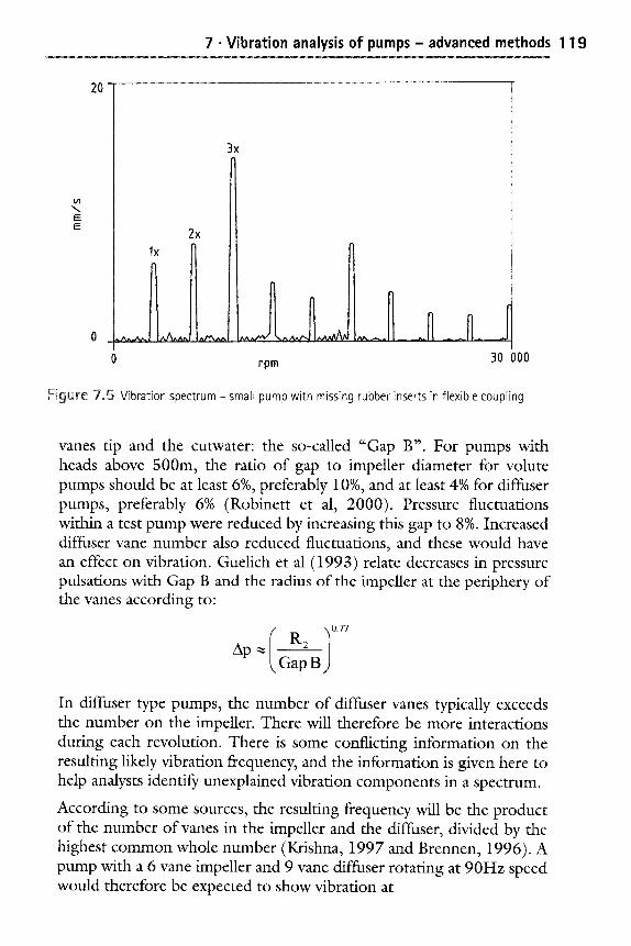
7 �9 Vibration analysis of pumps - advanced methods 1 19
E E
20-
3x
2x
Ix
0 rpm 30 000
Figure 7~ Vibration spectrum - small pump with missing rubber inserts in flexible coupling
vanes tip and the cutwater: the so-called "Gap B". For pumps with heads above 500m, the ratio of gap to impeller diameter for volute pumps should be at least 6%, preferably 10%, and at least 4% for diffuser pumps, preferably 6% (Robinett et al, 2000). Pressure fluctuations within a test pump were reduced by increasing this gap to 8%. Increased diffuser vane number also reduced fluctuations, and these would have an effect on vibration. Guelich et al (1993) relate decreases in pressure pulsations with Gap B and the radius of the impeller at the periphery of the vanes according to:
I 10.7 7 R2 Ap~ GapB
In diffuser type pumps, the number of diffuser vanes typically exceeds the number on the impeller. There will therefore be more interactions during each revolution. There is some conflicting information on the resulting likely vibration frequency, and the information is given here to help analysts identify unexplained vibration components in a spectrum.
According to some sources, the resulting frequency will be the product of the number of vanes in the impeller and the diffuser, divided by the highest common whole number (Krishna, 1997 and Brennen, 1996). A pump with a 6 vane impeller and 9 vane diffuser rotating at 90Hz speed would therefore be expected to show vibration at
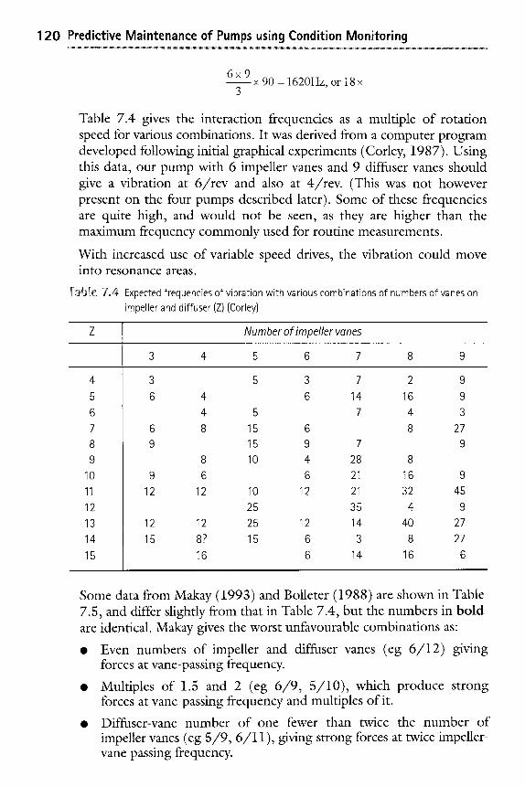
120 Predictive Maintenance of Pumps using Condition Monitoring
6x9 x 90 = 1620Hz, or 18 x
Table 7.4 gives the interaction frequencies as a multiple of rotation speed for various combinations. It was derived from a computer program developed following initial graphical experiments (Corley, 1987). Using this data, our pump with 6 impeller vanes and 9 diffuser vanes should give a vibration at 6 / rev and also at 4/rev. (This was not however present on the four pumps described later). Some of these frequencies are quite high, and would not be seen, as they are higher than the maximum frequency commonly used for routine measurements.
With increased use of variable speed drives, the vibration could move into resonance areas.
Table 7~4- Expected frequencies of vibration with various combinations of numbers of vanes on impeller and diffuser (Z) (Corley)
4
5
6
7
8
9
10
11
12
13
14
15
Number of impeller vanes
3 4 5 6 7 8 9
3 5 3
6 4 6
4
6 8
9
9
12
12
15
8 6
12
12
8?
16
7 2 9
14 16 9
5 7 4 3
15 6 8 27
15 9 7 9
10 4- 28 8
6 21 16 9
10 12 21 32 45
25 35 4 9
25 12 14 40 27
15 6 3 8 27
6 14 16 6
Some data from Makay (1993) and Bolleter (1988) are shown in Table 7.5, and differ slightly from that in Table 7.4, but the numbers in bold are identical. Makay gives the worst unfavourable combinations as:
�9 Even numbers of impeller and diffuser vanes (eg 6 /12) giving forces at vane-passing frequency.
�9 Multiples of 1.5 and 2 (eg 6 /9 , 5 /10) , which produce strong forces at vane-passing frequency and multiples of it.
�9 Diffuser-vane number of one fewer than twice the number of impeller vanes (eg 5 /9 , 6 /11) , giving strong forces at twice impeller- vane passing frequency.

7 �9 Vibration analysis of pumps - advanced methods 121
Table '~ ~; z o,.0 Expected frequencies of vibration with various combinations of numbers of vanes on impeller and diffuser (Z) (Makay, Bolleter)
Number of impeller vanes
3 4 5 6 7
12
15
4 8,10 15
15
8 10
12
12
6 16
10
25
25
15
6
6,18,24 7
18 28
6 21
12 21
12 35
12 14
14
6 14
Makay gave a case study where vane combinations of 7/8 gave vibration of 8mm/s rms at 7x, as predicted by both the above tables (Makay 1995). Changing to an l 1-vane diffuser resulted in negligible vibration, despite reducing the impeller vane-diffuser gap from 21% to 15%. A vibration signature can show many components, and can make diagnosis difficult. Their sources cannot always be identified, but they should be noted for possible future correlation with an observed mode of degradation. Some will be resonances of components within the pump. As an example of the typical variations, Table 7.6 gives the key information from signatures taken on four 4-stage boiler feed pumps of the same type and size. The vibration on the same bearing on each pump was analysed to 6250Hz with constant bandwidth of 23.4Hz.
The slight differences in the pump operating speeds reflects slightly different flows and may have been sufficient to excite and reveal different internal resonances. These pumps have 6 vane impellers, 9 vane diffusers, and the 18x vibration is in agreement with Makay in Table 7.5. Vane-passing vibration of 6x and 4x as expected from Table 7.4 was not evident with either of these pumps. No information is available on their internal condition at the time of testing.
7 .6 .6 A c o u s t i c resonance
Acoustic resonance can occur when the speed of sound in the liquid and the length of the liquid path coincide with the wavelength. If this frequency coincides with that of a strong enough exciting force, high
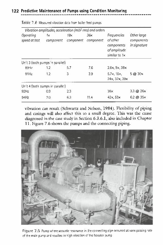
122 Predictive Maintenance of Pumps using Condition Monitoring ~ ,_ _ : - _ ~ - - -_,,~.~ ~ . ~ , - ~ . . ~ , . . ~
TabJe 7~ Measured vibration data from boiler feed pumps
Vibration amplitudes, acceleration (m/s 2 rms) and orders Operating lx 18x 36x speed at test component component component
Frequencies of other components of amplitude similar to lx
Other large components in signature
Unit 3 (both pumps in parallel)
89Hz 1.2 5.7
91Hz 1.2 3
7.6
3.9
2.6x, 9x, 38x
5.7x, lOx,
24x, 32x, 39x
5 @ 30x
Unit 4 (both pumps in parallel)
92Hz 0.9 2.3
94Hz 2.0 6.3 11.4
36x 3.3 @ 26x
42x, 53x 6.2 @ 35x
vibration can result (Schwartz and Nelson, 1984). Flexibility of piping and casings will also affect this to a small degree. This was the cause diagnosed in the case study in Section 6.3.6.1, also included in Chapter 11. Figure 7.6 shows the pumps and the connecting piping.
Fi~]ure 7.6 Pump where acoustic resonance in the connecting pipe occurred at vane passing rate of the main pump and resulted in high vibration of the booster pump
7 �9 Vibration analysis of pumps - advanced methods 1 2 3
The frequency of resonance in a pipe open to flow = v and its harmonics 2L
If the pipe is closed at one end, the frequency will be half of the above, and the odd harmonics will show, i.e.
V 3v 5V 4L' 4L' 4L
Where: L = length of pipe from noise source to where the geometry changes, such as an elbow or valve (m).
V = velocity of sound in the liquid (m/s) . In pure water, Vis in the range 1430 to 1590 m / s depending on the temperature. It is also affected by air content and pressure, and is greater in seawater.
In distilled water, at pressures up to 20 MPa and temperatures up to 100degC:
V= 1402.7 + 4 8 8 t - 482t2 + (15.9 + 2.8t +2.4 t 2 ) (P /10000) , where t is the temperature in degC/100 , and P the pressure in kPa.
At a more typical temperature for feed water pumps of 150degC, the sonic velocity varies linearly with pressure = 0.0022P + 1472.
The speed of sound in liquids is not readily available for all liquids (Robinett, 2000), but is given for estimation purposes within _+15% in metres/second f r o m - 9 . 3 4 6 SG 2 + 228.57 SG + 223.67, where SG is the Specific Gravity of the liquid.
The rigidity of the pipe also influences acoustic resonance. Guelich, et al 1993 gives this formula:
Speed of sound allowing for pipe rigidity = c o D pc~ 1 + ~ ~
h E Where, in consistent units:
Co = speed of sound in water for infinitely rigid pipe D = average diameter of pipe (i.e. diameter at mean wall
thickness) h - wall thickness of pipe 9 = density of pipe material E = modulus of elasticity for the pipe material
Design handbooks show how to calculate the natural frequencies of piping. These vary with material, section size, end fastening and temperature and obviously must not coincide with the likely exciting frequencies mentioned earlier.
124 Predictive Maintenance of Pumps using Condition Monitoring
7~ Vertical pumps
Vertical pumps, particularly the long spindle multistage type, have interesting vibration characteristics. These are usually essentially a cantilever, supported on a base plate. Access for vibration measurement is limited, and routine measurements must be made on the motor flange/s, as shown in the Standards listed in Chapter 6. It may be decide to mount a transducer permanently nearer the impellers.
The natural frequency of such pumps, sometimes called "reed frequency", can often be below running speed. Stiffening, mass changes, and absorbers have all been used to cure vibration during commissioning. Looseness, particularly of mounting bolts, can allow the pump column to vibrate at its natural frequency.
7.8 Effect of internal wear on vibration
Internal wear within a pump can change the flow patterns and change the vibration pattern. Erosion and looseness can change the resonances of pump and its components, and these would be expected to show in the vibration spectrum.
It seems that more field experience with particular pumps is needed to reliably relate internal wear with spectral vibration changes. Careful tests were arranged during development of a 6-stage pump (750m3/h @1788m at speed of 5000 r /min) (France, 1990). Tests were run with no changes other than three increasing annular clearances" design, 1.5 and 2 times design. Subsynchronous vibration only appeared with twice design clearance, at higher speeds, at 0.84• and locked on as speed was raised.
With increasing wear of multistage pumps, the bearing effect exerted by the wearing rings can weaken, such that the first critical speed moves down nearer to the operating range, or even to within it. Increasing leakage can reduce the damping, widening the speed range at which the critical speed appears (Nelson, 1987; Pace et al 1986).
7.8.1 Case study
Vibration increased steadily on the NDE bearing of a boiler feed pump, 4 stage, constant speed 5800 r /min, as shown in Figure 7.7. Frequency analysis showed that virtually all of the vibration was at l x, and experience had related this to internal wear. As a standby pump was not
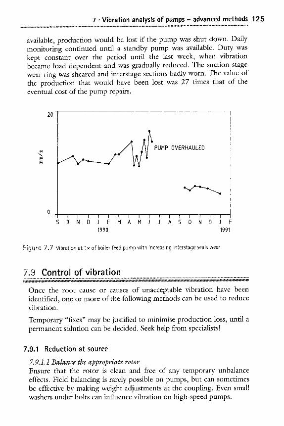
7 �9 Vibration analysis of pumps - advanced methods 1 2 5
available, production would be lost if the pump was shut down. Daily monitoring continued until a standby pump was available. Duty was kept constant over the period until the last week, when vibration became load dependent and was gradually reduced. The suction stage wear ring was sheared and interstage sections badly worn. The value of the production that would have been lost was 27 times that of the eventual cost of the pump repairs.
E E
20
PUMP OVERHAULED
I i I I I I I ~ I I I " i I " I I I I S 0 N D J F M A M J J A S 0 N D J -
1990 1991
Figure 7.,7 Vibration at Ix of boiler feed pump with increasing interstage seals wear
7,9 Control of vibration
Once the root cause or causes of unacceptable vibration have been identified, one or more of the following methods can be used to reduce vibration.
Temporary "fixes" may be justified to minimise production loss, until a permanent solution can be decided. Seek help from specialists!
7.9.1 Reduction at source
7.9.1.1 Balance the appropriate rotor Ensure that the rotor is clean and free of any temporary unbalance effects. Field balancing is rarely possible on pumps, but can sometimes be effective by making weight adjustments at the coupling. Even small washers under bolts can influence vibration on high-speed pumps.
126 Predictive Maintenance of Pumps using Condition Monitoring
7.9.1.2 Balance magnetic forces Balance magnetic forces in motors by adjusting the air gap clearances or correctly setting the rotor axial magnetic centre, where possible.
7. 9.1.3 Correct clearances Correct clearances or looseness.
7.9.1.4 Reduce aerodynamic effects An example given earlier for pumps with diffuser vanes where the clearance between impeller vane tips and stationary parts can be increased, without affecting pump performance.
7.9.2 Isolation
7.9.2.1 Isolate the source Isolate the source, using isolating mountings. Application details are available from mounting manufacturers. Flexible piping sections may help.
7. 9.2.2 Isolate affected equipment Isolate affected equipment or areas, to remove the effect of forced vibration from external sources.
7.9.3 Reduction of the response
7. 9.3.1 Alter the natural frequency Alter the natural frequency of the structure, by changing its stiffness or mass (see the fundamental equation in Section 7.4). Changes of about 50% may be needed to be effective:
If the natural frequency is above the vibration forcing frequency, then increasing the stiffness, or decreasing the mass, will raise the natural frequency and lower the response at the exciting frequency.
If the natural frequency is below the vibration forcing frequency, then reducing the stiffness, or increasing the mass will lower the natural frequency further to lower the response.
Modal analysis using a combination of vibration measurement, testing, analysis and software, is used to solve more complex vibration problems. Terms such as Operational Deflection Shapes and the Frequency Response Function are used.
7. 9.3.2 Increase damping Increase damping in the system. Damping coatings, or a dashpot (such as large "shock absorbers") may be appropriate.
7 �9 Vibration analysis of pumps - advanced methods 1 2 7 - - ~ ~ ~ . ~ , ~ . ~ . . . . ~
7. 9.3.3 Use a dynamic vibration absorber to detune the system This is an auxiliary mass coupled to the system by springs and tuned to vibrate at the natural frequency. Two new resonances are created that replace the original: one above and one below it. These new resonances should not coincide with any vibration of the same frequencies. Details are given in vibrations textbooks, and trial and error experimentation may be cost-effective once the approximate size is selected, and the final bandwidth must allow for any variation in frequency of the driving force.
7oi0 Setting band levels for monitoring
Comparing spectra taken at time intervals under similar loading conditions will reveal any changes at specific frequencies. When this method was first developed, manual comparison was used, but this is slow, monotonous and cumbersome. Today's computer-based systems handle this with ease, and detailed advice can be expected with purchase of such a system. As even constant speed machines vary slightly in speed, analysis With a high number of lines may allow vibration components to slip into a frequency bin either side of the normal value and be missed. Analysis referred to a l x shaft marker will overcome this problem. Constant percentage filters can cope with such speed variations.
Some pump engineers consider that as higher frequency vibrations result in lower displacements and stresses relative to a constant vibration velocity, higher allowable vibration velocity may be allowed at higher frequencies. Also, as there is tittle or no literature about failures resulting from discrete higher frequency vibrations of shafts, bearings, mechanical seals, auxiliary piping, etc., overall levels are suggested as limits for severity assessment (Robinett and Kaiser, 2000).
However, as monitoring in discrete frequency bands gives a greater insight into the internal condition of a pump, limits for action and correlation are worthwhile. A practical way from experience of deciding which frequency ranges to monitor and relevant alarm levels is given by Berry (1990). Table 7.7 shows his recommended settings for centrifugal pumps.
7.11 Permanent monitoring of pumps
For most process pumps, routine vibration data collection and analysis at intervals of a month to three months have been found sufficient,
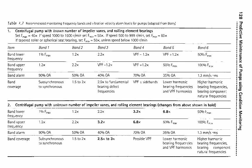
128 Predictive M
aintenance of Pumps using C
ondition Monitoring
~.
.~
:
..
..
~
..~
~_
. :
..
..
.
. ..
..
.
..
>,.
r,n
E o r E o r E fj _s c- o ,m
c c-
d')
>.. fj c-
-m
r o c- o
E
-c~ c-
E E o
X O t,,.O
II >
ii r
i./'i
.E E
O'~
O~
O
O O LO
c')
X O II >
E ii iz#
.E E
O O O
O O O r X O II >
ii
1.0
q:l
E ii
O X o,,I
-I- ii X oq I
ii X X O,I E ii ~
J
06
r
x E
ii O
O x c~ E
ii O
X
CN
+ ii r~ X
I ii rl X
C
N
X
~4
,I---
~J
og
c
-
t~
E
E
E
m
o o 0 t~
o 0
o 0
o 0 E
"o
c-
_L
.~
._
0
c--
.,_, ~-~
IZ)
~ c
- __J
..0
c~
-o
c--
..o
t~
+1 ii
m c
-
E
.~
o~6
c,i _o
~
X
~4
0
L~
o~ O
0 c- O
c
-
c-
..om
6,~
r
2, ~
O
~Z
O
O
IE O
4-
,m
IE
C
O
IE o~
O
IE ~Z
O IE
,m
I=
E ii
O L.O
x X X o,I
X o,I
~b
06
c-
x E
LI_
O
O x E
u
_
O
L.O
x X
X
o,I
o,,I
X
o,,I
"b
--,6 c-
E
E
E
<(
o o 0
<(
o 0
<(
o 0
o 0 E
c-
C~
(--
E
cr~
~ g
c'- ~._
~_
"m
~, ~
~Y
E
E
cr ~
~ ._
>
<S) ~
C
_._1 _
.0
c'~
ii E
L
GJ
..O
.m
t/3 t/3 O
C
L
X
r O
4-a
X
LO
r X
c'q
O
IF)
u3
O
O
c-
~-
O
c-
~.- r
c-
c-
r
_o
~o
0J
co
<1.) ~> O
(J
c- ('o
rv~

7 �9 Vibratio
n
analysis of pum
ps - ad
vanced
m
etho
ds
12
9
e- ,m
e-
e-
._e ~
o
..O
.m
"~
U_
"
E ~
"~
E
e-
~ tm
X
+
ii X I
ml
121..
X
~')
x X
o >
-og C
ea~
x E
LL
o o X
+
ii 121._
X
('M
I
I_i._
x C
O
X
X
-,.5
O
o
O
o P~
O
o C~
O
(s)
O
o
O
o C??
E
O
E~
c--
..O
+1 im
X
O
X
O
o e-
e.-
o e-
o E
o L_
e-
e"
~7
e"
,m e"
e-
E
O
L_
E
e-
o e-
E
,m e-
x x X
m.
x
,e.--
x
c
) r
Ii c-- g
E
I..L
o o x x X
X
OO
X
o -,.5 -og C
O
o
o o O
o
O
o
O
o E
C
X
E
IL
O x x o • X
o X
X
LO
O
X
X
O
x O
O
c--
O
C.)
"O
c--
r~
0J C
J
0 u3
~J
c-
O
0 bq
-0
(13
c-
(13
c-
c-
0 0
"~
o3
-0
4-~
o 0
~J
v1
~_
c-
_0
0 u
3
o
E
c- r
r c
-
O-
"~
co
r E3"
o3
4
--
o ~
o O
c c'~
C
~ >
>-
E
m
m
._m
_. _-~
,---
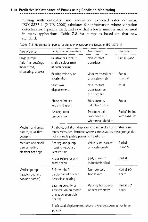
130 Predictive Maintenance of Pumps using Condition Monitoring
varying with criticality, and known or expected rates of wear. ISO13373-1 (FDIS 2003) tabulates for information where vibration detectors are typically used, and says that a lesser number may be used in many applications. Table 7.8 for pumps is based on that new standard.
TabJe 7.8 Guidelines for pumps for vibration measurements (based on ISO 13373-I)
Type of pump Evaluation parameters Transducer Direction
Large pumps, fluid-film bearings (boiler feed, circulating, process)
Relative or absolute shaft displacement at each bearing
Bearing velocity or acceleration
Shaft axial displacement
Phase reference and shaft speed
Bearing metal temperature
Non-contact Radial +45 o transducer
Velocity transducer Radial, or accelerometer H and V
Non-contact transducer on thrust collar
Eddy current/ inductive/optical
Thermocouple embedded into whitemetal (Babbitt)
Axial
Radial
Radial, in line with load line
Medium and small pumps, fluid-film bearings
As above, but shaft displacement and metal temperatures are rarely measured. Portable systems are usual, as these pumps do not normally justify permanent systems.
Medium and small pumps, rolling element bearings
Bearing and pump Velocity transducer Radial, housing velocity or or accelerometer H and V acceleration
Phase reference and Eddy current/ Radial shaft speed inductive/optical
Vertical pumps (reactor coolant, coolant pumps)
Relative shaft displacement at each accessible bearing
Non-contact Radial 900 transducer apart
Bearing velocity or acceleration on motor and each accessible bearing
Velocity transducer Radial 900 or accelerometer apart
Shaft axial displacement, phase reference, speed as for large pumps
7 �9 Vibration analysis of pumps - advanced methods 131
Based on risk assessment, pumps may justify permanent monitoring systems according to the criticality of their service, consequence of failure, severity of service sensitivity of a pump's design to damage (Karassik and McGuire, 1998). Other permanent monitoring in addition to that in Table 7.7 can include measurement of pump suction condition, minimum flow, seal injection, lubricant supply, seal condition, casing temperature, balancing device leakoff flow, pump flow and speed. Monitoring systems are available to use all available information from a plant's DCS and detect differences between normal variations in operating conditions and changes in equipment condition. Sensor faults can also be detected (see Chapter 3).
The minimum monitoring system would have accelerometers mounted on the drive end bearings of driver and pump.
Locally mounted signal conditioning can transmit a 4-20mA signal to a PLC or to control room indications, but frequency analysis cannot be made from such signals.
Some power plants have fitted torquemeters to measure power input of steam driven pumps. Hogging of the casing can be a problem on longer pumps operating at high temperature. Thermocouples fitted to measure the top and bottom temperatures provide operator guidance.
Analysis of failure statistics collected by service units and operators (Berge, 2003) shows that two or three sensors are sufficient for pump monitoring and much diagnosis: to detect dry running, measure the beating temperature and monitor the vibration level. For maximum benefit, the information presented for decision making must be more than just a display or collection of numbers from individual transducers. The outcome of such analysis will surely be more powerful and accurate decision support systems, as mentioned elsewhere in this book.
References
API 610 (1995) Centrifugal pumps for refinery service 8th edition, American Petroleum Institute, Washington 1995 (9th Edition due 2003: Centrifugal pumps for the petroleum, petrochemical and natural gas industries) [Standard]
Beebe, RS (2001) Machine condition monitoring, MCM Consultants. ISBN 0646250884 [Book]
Berge, G (2003) The pump as a condition indicator World Pumps, June [Article]
132 Predictive Maintenance of Pumps using Condition Monitoring
Berry, JE (1999) Proven method for specifying spectral band alarm levels and frequencies using today's predictive maintenance software systems 4th Ed Technical Associates of Charlotte [Booklet]
Bloch, HP et al: Practical Machinery Management for Process Plants Gulf, 1982, etc. (Four volumes) ISBN 0872013766, 0872018725, 0872016757, 0872014541 [Books]
Bolleter, U (1988) Blade-passing tones of centrifugal pumps Vibrations, Vol 4 (3), Sep [Article]
Brennen, CE (1996) Hydrodynamics of pumps Concepts ETI, Oxford University Press [Book]
Buscarello, R (2001) Practical solutions to machinery vibration problems [Course Notes]
Corley, JE (1987): Tutorial session on diagnostics of pump vibration problems Proceedings of the 4th International Pump Symposium, Texas A&M University [Paper]
Gopalakrishnan, S (2000) Software base diagnosis of feed pump problems Proceedings of MARCON 2000, Knoxville [Paper]
Guelich, JF; Bolleter, U; Simon, A (1993) Feedpump operation and design guidelines EPRI TR- 102102 [Book]
France, D and Taylor, PW (1990): Near running speed synchronous vibration in centrifugal pumps IMechE Seminar, Vibrations in Centrifugal Pumps 1990 [Book]
Goldman, S (1999) l/Tbration spectrum analysis- a practical approach 2nd Ed Industrial Press, NY [Book]
Hines, JW; Jesse, J; Kuropatwinski, J; Carley, T; Kuseck, J; Nower, D and Hale, F (1997) Motor shaft alignment versus efficiency analysis P/PM Technology, October [Paper]
Hines, JW; Jesse, J; Edmondson, A (1999) Study shows shaft misalignment reduces bearing life Maintenance Technology, April [Article]
ISO13373-1 (FDIS 2003) Condition monitoring and diagnostics of machines- Vibration condition monitoring - Pt 1: General procedures [Standard]
ISO 1940/1-1986 Mechanical vibration - Balance quality requirements of rigid rotors - Pt I [Standard]
Jesse, S; Hines, JW; Edmondson, A and Nower, D (1999) Motor shaft misalignment bearing load analysis Proceedings of MARCON 99, Knoxville [Paper]
Karassik, I J and McGuire, T (1998) Centrifugalpumps Prentice-Hall [Book]
Kataoka, T; Yamashina, C, and Komatsu, M (1987) Development of an incipient failure detection technique for mechanical seals Proceedings of 4th International Pump Symposium Texas A&M University [Paper]
7 �9 Vibration analysis of pumps - advanced methods 1 3 3 �9 . ~ -~ ~ . - ~ -~ .~ . - ~ �9
Krishna, Radna HC (Ed) (1997) Hydraulic design of hydraulic machines Avebury, Aldershot [Book]
Lee, YB; Lee, TW; Kim, SJ; Kim, CH and Rhim, YC (2001) A hybrid knowledge-based expert system for rotating machinery Proceedings of 14th International Congress of COMADEM, Elsevier [Paper]
Makay, E and Hogan, J (1993) Be aware of acoustic resonances in pump vane/impeller problems POWER Feb [Article]
Makay, E; Gates, W, Blair, B (1995) Acoustic resonance fix halts feed-pump vibration POWER Feb [Article]
Marscher, W and Campbell, J (1998): Methods of investigation and solution of stress, vibration and noise problems in pumps Proceedings of 15th International Pump Symposium Texas A&M University [Paper]
Mitchell, JS (1993) Introduction to Machinery Analysis and Monitoring 2nd Ed PennWell [Book]
Myers, RD (1995) Minimize pump downtime Hydrocarbon Processing, June, Vol 74 No 6 [Article]
Nelson, WE (1987) Pump vibration analysis for the amateur Proceedings of 4th International Pump Symposium Texas A&M University [Paper]
Nevlik, L and Jackson, C (1995) Effect of mechanical unbalance on vibrations, forces and reliability of a single-stage centrifugal pump Proceedings of 12th International Pump Symposium Texas A&M University [Paper]
Pace, S; Florjancic, S; Bolleter, U (1986) Rotordynamic developments for high speed multi-stage pumps Proceedings of 3rd International Pump Symposium Texas A&M University [Paper]
Robinett, FL; Gulich, JF and Kaiser, T (2000): Vane pass vibration: source, assessment and correction - A Practical Guide for Centrifugal Pumps: Part 1 RELIABILITY magazine, Feb [Paper]
Robinett, FL; and Kaiser, T (2000): Vane pass vibration: source, assessment and correction - A Practical Guide for Centrifugal Pumps: Part 2 RELIABILITY magazine April [Paper]
Sawyer, J (1980) Sawyer's Turbomachinery Handbook, Turbomachinery International Publications [Book]
Schwartz, RE and Nelson, WE (1984) Acoustic resonance phenomena in high energy variable speed centrifugal pumps Proceedings of 1st International Pump Symposium Texas A&M University [Paper]
Sikorska, J and Pan, J (2003) A review of acoustic emission techniques for the diagnosis of faults in rotating machinery Proceedings of ICOMS2003 International Conference of Maintenance Societies, Perth, May [Paper]
134 Predictive Maintenance of Pumps using Condition Monitoring
Technical Associates of Charlotte: Diagnosis of machine faults wall chart (also in Mitchell, 1993) and interactive software version (www.technicalassociates. net) [ Software ]
Wang, L; Hope, AD; Sadek, H (2001) Multi-layer neural networks and pattern recognition for pump fault diagnosis Proceedings of the 14th International Congress of COMADEM, Elsevier [Paper]
www.iLearnInteractive.com [Website]
www.hanetraining.com/bearexpert.html [Website]
www.fag.de/NASApp/[Website]
www.pruftechnik, co.uk/[Website]
Yoshida, Y et al (1998) Unbalanced hydraulic forces caused by geometrical manufacturing deviations of centrifugal impellers ASME Journal of fluids engineering Vol 120, Sep [Paper]
Bibliography
Crawford, Art (1992) The simplified handbook of vibration analysis (2 vols) CSi
Mobley, K (1991) Introduction to Predictive Maintenance Technology for Energy
Taylor, James (1994) The vibration analysis handbook Vibration Consultants Inc
Wowk, V (1994) Machine Vibration- balancing McGraw-Hill ISBN 0070719381
Wowk, V (1991) Machinery Vibration -Measurement and Analysis McGraw- Hill
Other uses of eond ition mon itori ng information
W Tuning a pump system m Impeller trimming: Medium size pump - 132kW
Impeller trimming: large size pump - 1320kW W Condition monitoring of shaft seals E Monitoring of seal-less pumps
8,1 Tuning a pump system
When selecting a pump, the designer assumes a piping condition, and allows margins on head and flow to be sure that the pump will meet design requirements. But, when the plant is built and put into service, this may mean that the pump is oversized. As an example, the results of a survey in Finland by Jantunen (2000) gave the average overall pumping efficiency as less than 40%. Pumps consume about 10% of the total electricity in Finland, so the wastage is very high. The US Department of Energy estimates that 5% of all power is consumed by pumps and that a 20% reduction is possible (HI, 1997). A similar situation can be expected in other countries.
In this chapter, we look at two examples of different sizes and types of pump, and show how performance analysis of even a medium size pump can give large savings if a smaller diameter impeller is sufficient for the required duty. Impellers can be machined down for radial-flow and to a limited extent with mixed-flow pumps. Reducing the diameter of star vane impellers of side channel pumps is not possible (SIHI, 1988).
There are other efficiency improvement measures. Modern software facilitates speedy checks of the system design, to evaluate the effect of
136 Predictive Maintenance of Pumps using Condition Monitoring
such changes as diffuser entry-exit sections at pipe-tank connections. Variable-speed drives and adding a smaller pump for use where the required flow is sometimes less, are two other examples.
As shown in Chapter 4, condition monitoring by performance analysis can also provide the information to determine when overhaul of a pump to restore worn clearances is justified on an energy cost basis.
8.2 Impeller trimming" Medium size pump- 132kW
8.2.1 Design selection
A plant system handling clean water requires a flow of 615m3/h . With a static head of 37m, adding the calculated frictional resistance gives a total head at this flow of 55m. With the usual design margins added, a constant speed pump with a 375mm diameter impeller was selected to meet this duty: see Head-Power-Flow curves "375~" on Figure 8.1. This pump has a Specific Speed of 1920 (US units).
8.2.2 Operation in service
When the pump is in service, it must be throttled on discharge to keep the flow down to the required 615m3/h. A head-flow test shows that the operating point is A, at a head of 64m. From the Power-Flow curve in Figure 8.1, the pump absorbs 123kW.
The actual system curve was found on test by running the pump unthrottled, measuring the suction and discharge pressures and the flow. As explained in earlier chapters, for such tests velocity head is allowed for if the suction and discharge pipes are of different diameters at the points of pressure measurement. If the gauges are not at the same level, readings are corrected to allow for static leg.
The system static h e a d - the zero flow p o i n t - is found from site measurements or plant elevation drawings. In this example, the operating point, unthrottled, is found to be 725 m3/h @ 60m, so the actual system curve B is lower than design expectations. The required operating p o i n t - the total system resistance for the desired f l o w - is therefore 615 m3/h@ 53m. For this discussion, these are designated /-/]and Q3.
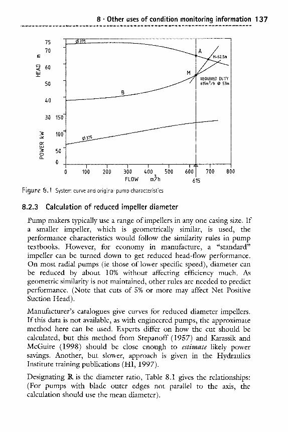
8 �9 Other uses of condition monitoring information 137
75
70
E
o 60 < UJ -r-
50
~o
30 150-
100- r~ : ~ 50 0
0 .
A
~ / ] REQUIRED DUTY 615m3/h @ 53m
.............. I .................... I ........ I .................. I .... I ; I
0 100 200 300 /,00 500 600 FLOW m~'h
Figure 8ol System curve and original pump characteristics
700
615
800
8.2.3 Calculation of reduced impeller diameter
Pump makers typically use a range of impellers in any one casing size. If a smaller impeller, which is geometrically similar, is used, the performance characteristics would follow the similarity rules in pump textbooks. However, for economy in manufacture, a "standard" impeller can be turned down to get reduced head-flow performance. On most radial pumps (ie those of lower specific speed), diameter can be reduced by about 10% without affecting efficiency much. As geometric similarity is not maintained, other rules are needed to predict performance. (Note that cuts of 5% or more may affect Net Positive Suction Head).
Manufacturer's catalogues give curves for reduced diameter impellers. If this data is not available, as with engineered pumps, the approximate method here can be used. Experts differ on how the cut should be calculated, but this method from Stepanoff (1957) and Karassik and McGuire (1998) should be close enough to estimate likely power savings. Another, but slower, approach is given in the Hydraulics Institute training publications (HI, 1997).
Designating R is the diameter ratio, Table 8.1 gives the relationships: (For pumps with blade outer edges not parallel to the axis, the calculation should use the mean diameter).
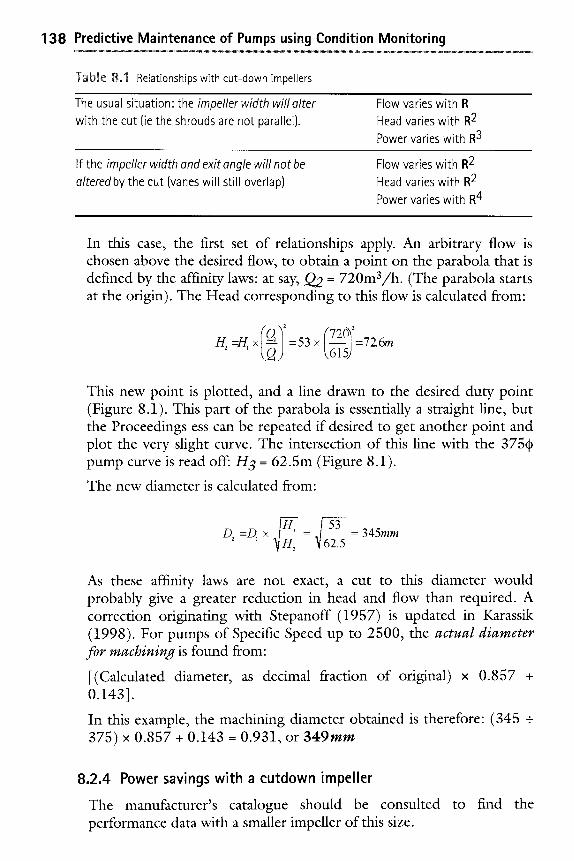
138 Predictive Maintenance of Pumps using Condition Monitoring
Tabte 8.1 Relationships with cut-down impellers
The usual situation the impeller width will alter with the cut (ie the shrouds are not parallel).
Flow varies with R Head varies with R 2 Power varies with R 3
If the impeller width and exit angle will not be alteredby the cut (vanes will still overlap)
Flow varies with R 2 Head varies with R 2 Power varies with R 4
In this case, the first set of relationships apply. An arbitrary flow is chosen above the desired flow, to obtain a point on the parabola that is defined by the affinity laws: at say, Q2 = 720m3/h. (The parabola starts at the origin). The Head corresponding to this flow is calculated from:
H 2 =H 1 x -53 x I720~2:726m <615.)
This new point is plotted, and a line drawn to the desired duty point (Figure 8.1). This part of the parabola is essentially a straight line, but the Proceedings ess can be repeated if desired to get another point and plot the very slight curve. The intersection of this line with the 375~ pump curve is read off: H 3 = 62.5m (Figure 8.1).
The new diameter is calculated from:
D 2 =D, x = = 345mm 62.5
As these affinity laws are not exact, a cut to this diameter would probably give a greater reduction in head and flow than required. A correction originating with Stepanoff (1957) is updated in Karassik (1998). For pumps of Specific Speed up to 2500, the actual diameter for machining is found from:
[(Calculated diameter, as decimal fraction of original) x 0.857 + 0.143].
In this example, the machining diameter obtained is therefore: (345 + 375) x 0.857 + 0.143 = 0.931, or 3 4 9 m m
8.2.4 Power savings with a cutdown impeller
The manufacturer's catalogue should be consulted to find the performance data with a smaller impeller of this size.
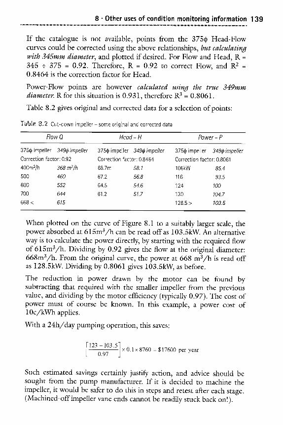
8 �9 Other uses of condition monitoring information 139
If the catalogue is not available, points from the 375~ Head-Flow curves could be corrected using the above relationships, but calculating with 345mm diameter, and plotted if desired. For Flow and Head, R = 345 + 375 -- 0.92. Therefore, R- - 0.92 to correct Flow, and R 2 - 0.8464 is the correction factor for Head.
Power-Flow points are however calculated using the true 349mm diameter. Rfor this situation is 0.931, therefore R 3 -- 0.8061.
Table 8.2 gives original and corrected data for a selection of points"
Tabte 8.2 Cut-down impeller - some original and corrected data
Flow Q Head- H Power- P
375~ impeller 3494)impeller 375~ impeller 349q~impeller 375~ impeller 3494)impeller Correction factor: 0.92 Correction factor: 0.8464 Correction factor: 0.8061
400m2/h 368 m2/h 68.7m 58.1 106kW 85.4
500 460 67.2 56.8 116 93.5
600 552 64.5 54.6 124 100
700 644 61.2 51.7 130 104.7
668 < 615 128.5 > 103.5
When plotted on the curve of Figure 8.1 to a suitably larger scale, the power absorbed at 615m3/h can be read off as 103.5kW. An alternative way is to calculate the power directly, by starting with the required flow of 615m3/h. Dividing by 0.92 gives the flow at the original diameter: 668m3/h. From the original curve, the power at 668 m3/h is read off as 128.5kW. Dividing by 0.8061 gives 103.5kW, as before.
The reduction in power drawn by the motor can be found by subtracting that required with the smaller impeller from the previous value, and dividing by the motor efficiency (typically 0.97). The cost of power must of course be known. In this example, a power cost of 10c/kWh applies.
With a 24h/day pumping operation, this saves:
123 - 103.5
0.97 • O. 1 x 8760 = $17600 per year
Such estimated savings certainly justify action, and advice should be sought from the pump manufacturer. If it is decided to machine the impeller, it would be safer to do this in steps and retest after each stage. (Machined-off impeller vane ends cannot be readily stuck back on!).
140 Predictive Maintenance of Pumps using Condition Monitoring
If a particular pump is known t o wear rapidly, or the frictional resistance in the system it supplies increases due to internal deposition, then the smallest impeller calculated this way may not be appropriate. Some performance margin may be justified. Another possibility would be to order another impeller for the present actual duty, and keep the original size one in store just in case. An alterative narrower impeller may be available. The cost of a new impeller in this example would be recovered in a few weeks.
The reduced power required may enable a smaller motor to be used. Further energy savings could result if this runs nearer its rated output. Even though motor efficiencies may be similar, less overall losses in kW will occur with a smaller motor required to give the same output at the same motor efficiency (www.motor.doe.gov/mchal.shtml). A high efficiency motor would give further energy savings.
Incidentally, the effects of changes in speed follow the same affinity laws as when the impeller width alters with a diameter cut. The same method is used as above, but using speed in place of diameter in the steps given. The correction to impeller diameter for machining does not of course apply in this case. It is possible to change both diameter and speed together to obtain a desired performance characteristic.
8=3 Impeller trimming" large size pump - 1320kW
8.3.1 Design selection
In this case, there are two power station cooling water pumps in parallel (2 x 50% capacity), each selected to supply a total flow of 4.675 m3/s at a design head of 24.5m. The combined flow must not be exceeded or unacceptable erosion of condenser tubes is likely. The pumps are single- stage, with double entry impellers of 986mm outside diameter. The impeller shrouds are not parallel. Motor efficiency is 95.3%.
8.3.2 Operation in service
Site tests were run to develop condition monitoring. They revealed that the system resistance was only 21.6m, much less than design, such that the flow must be restricted by partly closing the outlet isolating valves.
The original Head-Flow and Power-Flow curves for one pump are shown in Figure 8.2. The duty points are shown as "Design" and "Actual".
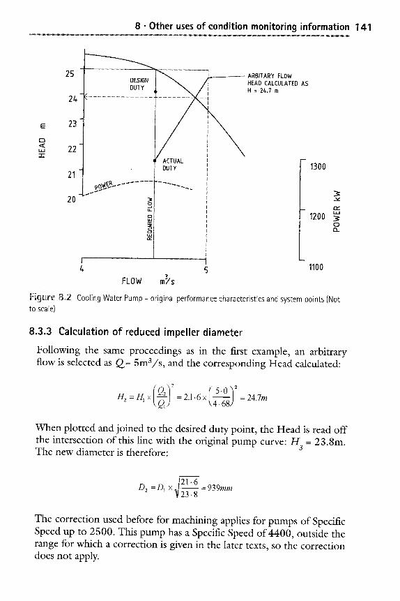
8 �9 Other uses of condition monitoring information 141
25
24
23
C~ < ,,, 22 - r -
21
20
T,
DESIGN DUTY
3~ O
t,L
Q
; ARBITARY FLOW j HEAD CALCULATED AS i H = 24.7 m
ACTUAL DUTY 1300
u j 1200 :~
CD (3_
I . . . . m
/+ 5 1100
FLOW m~'s
Figure. 8.2 Cooling Water Pump - original performance characteristics and system points (Not to scale)
8.3.3 Calculation of reduced impeller diameter
Following the same proceedings as in the first example, an arbitrary flow is selected as Q= 5m3/s, and the corresponding Head calculated-
H 2 H1 • Q 2 2 = = 2.1.6 • = 24.7m 4 .68
When plotted and joined to the desired duty point, the Head is read off the intersection of this line with the original pump curve" H = 23.8m. The new diameter is therefore- 3
D2 =D1 • V 23 8
= 939mm
The correction used before for machining applies for pumps of Specific Speed up to 2500. This pump has a Specific Speed of 4400, outside the range for which a correction is given in the later texts, so the correction does not apply.
142 Predictive Maintenance of Pumps using Condition Monitoring
As this is an engineered pump, manufacturers catalogue data is not likely to be available, and some points from the existing Head-Flow curves could be corrected using the above relationships, based on the first calculated diameter (ie 939mm) and plotted if desired.
8.3.4 Power savings with eutdown impeller
From the Power-Flow curve when plotted, the power saved for the required duty flow with a cut-down impeller was estimated as in the first example"
1253 - 1097 ] _ 164 kW saved per pump 0.953 3
With two pumps operating 90% of the year, this totals 2586MWh, equivalent to $103 000 at an average selling price of 4c/kWh.
The impact would of course be proportionally greater with a higher selling price, or if the power was bought in. Such estimated savings in energy cost and in matching greenhouse emissions certainly justify action, and the advice of the pump manufacturer should be sought. Proceedings to machine such a large impeller without reference is not recommended.
8.4 Condition monitoring of shaft seals
On pumps with labyrinth type seals, wear is indicated by increased seal flow. Monitoring facilities may be provided, or a pipe surface flow meter used. Leakage to outside the pump may be able to measured directly with a container.
Mechanical seals are widely used on pumps, and give good service when cared for. Failures still occur, and are often associated with high vibration (Bloch and Geitner 1994a) In the petro-chemical industry, up to 70 percent of the cost of pump repairs is spent on seals, and thorough trouble-shooting is well justified (Bloch and Geitner 1994b). Development of better designs and materials proceeds (Netzel and Sabina, 2002). An excellent description of seal types and analysis of failure is given by Bachus and Custodio (2003).
High vibration and seal failures were related in a study of 500 process pumps (Bloch and Geitner, 1994b).
Axial vibration at vane passing frequency does relate to seal failure, not lateral vibration (Robinett, 2000).
but
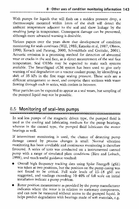
8 �9 Other uses of condition monitoring information 143
With pumps for liquids that will flash on a sudden pressure drop, a thermocouple mounted within lmm of the shaft will detect the ambient temperature adjacent to the seal and show leakage by the resulting jump in temperature. Consequent damage can be prevented, although more advanced warning is desirable.
Various papers over the years show that development of condition monitoring for seals continues (Will, 1985; Kataoka et al, 1987; Olmos, 1990; Kovach and Paranag, 2000, Schmidthals and Greitzke, 2001). Acoustic emission is a promising method for detection of abnormal wear or cracks in the seal face, as is direct measurement of the seal face temperature. Seal OEMs may be expected to make such systems available. The SmartSignal eCM system has been used to give early warning of seal degradation on a reactor coolant pump, by identifying a shift of 35 kPa in the first stage sealing pressure. These seals are a different arrangement to most, and comprise three sections with water flowing through each in series, with coolers in between.
Wear particles can be expected to appear as a seal wears, but sampling of the pumped liquid may not be possible.
8~ Monitoring of seal-less pumps
In seal-less pumps of the magnetic driven type, the pumped fluid is used as the cooling and lubricating medium for the pump bearings, whereas in the canned type, the pumped fluid lubricates the motor bearings as well.
If intermittent monitoring is used, the chance of detecting pump damage caused by process changes is small. Normal vibration monitoring has been unreliable and continuous monitoring is therefore favoured. A series of tests was conducted on a instrumented canned pump with a range of simulated plant conditions (Bleu and Lobach, 1998), and much useful guidance resulted"
�9 Overall high frequency tracking data using Spike Energy| (gSE) was taken at two positions, but the position on the pump casing was not found to be critical. Full scale levels of 15-18 gSE are suggested, and readings exceeding 10-40% of full scale on initial installation indicate a pump problem.
�9 Rotor position measurement as provided by the pump manufacturer indicates where the rotor is in relation to stationary components, and can now be measured without access to the pumped liquid. It helps predict degradation with bearings made of soft materials, e.g.
144 Predictive Maintenance of Pumps using Condition Monitoring
carbon/graphite, but does not help in predicting on hard bearings, such as of silicon carbide. Continuous monitoring of axial position was found to be more indicative, but both axial and radial are suggested. An increase of 50% on datum indicates bearing wear and maintenance should be scheduled. Catastrophic failure is likely at 70%.
References
Bachus, L and Custodio, A (2003) Know and understand centrifugal pumps Elsevier, UK [Book]
Bleu, JL and Lobach, J (1998) Continuous monitoring ofsealless pumps- the next step Proceedings of 15th International Pump Users Symposium, Texas A&M University [Paper]
Bloch, HP and Geitner, FK (1994a) Machinery failure analysis and troubleshooting (2nd Ed) Vol 2 of Practical Machinery Management for Process Plants, Gulf [Book]
Bloch, HP and Geitner, FK (1994b) An introduction to machinery reliability assessment (2nd Ed) Gulf [Book]
Department of Energy, USA Website: www.motor.doe.gov/mchal.shtml [Website]
Hydraulics Institute (1997) Energy reduction in pumps and pumping systems (Training package) USA
Jantunen, Errki et al (1998) Flexible expert system for the diagnosis of centrifugal pumps Proceedings of COMADEM 98 11th International Conference on Condition Monitoring and Diagnostic Engineering Management pp 433- 442 [Book]
Karassik, IJ and McGuire, T (1998) Centrifugal pumps Prentice-Hall [Book]
Kataoka, T; Yamashina, C; Komatsu, M (1987) Development of an incipient failure detection technique for mechanical seals Proceedings of 4th International Pump Symposium, Texas A&M University [Paper].
Kovach, JJ and Paranag, M (2000) Detection of impending mechanic seal failure in centrifugalpumps Proceedings of MARCON2000, Knoxville [Paper]
Netzel, JP and Sabini, EP (2002) Toward reduced pump operating costs, Part 3: Minimizing the effects of wear and optimising pump efficiency Proceedings of 19th International Pump Users Symposium, Texas A&M University [Paper]
Olmos, F (1990) Evolution of a mechanical seal condition monitoring system Proceedings 7th International Pump Users Symposium, Texas A&M University [Paper]

8 �9 Other uses of condition monitoring information 145
Stepanoff, A J (1957) Centrifugal and axial flow pumps Wiley [Book]
Schmidthals, C and Greitzke, SF (2001) Principles and application of a diagnostic system for mechanical seals Proceedings of 18th International Pump Users Symposium, Texas A&M University [Paper]
SIHI (1988) Basic principles for the design of centrifugal pump installations SIHI-Halberg [Book]
Will, T (1985) A powerful application and troubleshooting method for mechanical seals Proceedings of 2nd International Pump Symposium, Texas A&M University [Paper].
www.smartsignal, com/upload/appnotes/05.29.2003_Reactor%20 Pump %20A pp6.pdf [Note]
Other condition monitoring methods
m Visual inspection m Non-Destructive Testing ! Analysis of wear debris in lubricants
Other methods of condition monitoring associated with pumps
It will be evident by now that there is not a single one condition monitoring technique that will reveal all about the internal degradation of a pump. According to the mode, or modes, of degradation experienced or expected, other techniques may apply, where economically justified.
Simple techniques may suffice. If pump casing wear is a concern, and the liquid is not hazardous, a simple method is the self-indicating blind hole. It is drilled at the point of expected maximum wear to the depth corresponding to the minimum allowable casing thickness. When erosion has proceeded to this extent, liquid sprays out.
9.1 Visual inspection
A range of devices is available for internal visual inspection of machines, generally only possible when the machine is shut down and suitable access ports exist or can be arranged. If the observations are recorded for later comparison, then the rate of degradation could possibly be estimated by a suitably experienced person. In most cases, trending information is limited, but reassurance that an impeller is not damaged or fouled may be all that is required. Some devices are:
Optical boroscope: a rigid device, capable of good clarity. It cannot view at an angle to its axis unless an angled adaptor is fitted prior to inserting it.
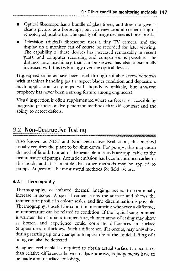
9 �9 Other condition monitoring methods 147
�9 Optical fibrescope has a bundle of glass fibres, and does not give as clear a picture as a boroscope, but can view around corner using its remotely adjustable tip. The quality of image declines as fibres break.
�9 Television (digital) fibrescope" uses a tiny TV camera, and the display on a monitor can of course be recorded for later viewing. The capability of these devices has increased remarkably in recent years, and computer recording and comparison is possible. The distance into machinery that can be viewed has also substantially increased with this technology over the optical devices.
High-speed cameras have been used through suitable access windows with machines handling gas to inspect blades condition and deposition. Such application to pumps with liquids is unlikely, but a c c u r a t e
prophecy has never been a strong feature among engineers!
Visual inspection is often supplemented where surfaces are accessible by magnetic particle or dye penetrant methods that aid contrast and the ability to detect defects.
9~ Non-Destructive Testing
Also known as NDT and Non-Destructive Evaluation, this method usually requires the plant to be shut down. For pumps, this may mean drained of liquid. Not all of the available methods are applicable to the maintenance of pumps. Acoustic emission has been mentioned earlier in this book, and it is possible that other methods may be applied to pumps. At present, the most useful methods for field use are:
9.2.1 Thermography
Thermography, or infrared thermal imaging, seems to continually increase in scope. A special camera scans the surface and shows the temperature profile in colour scales, and fine discrimination is possible. Thermography is useful for condition monitoring whenever a difference in temperature can be related to condition. If the liquid being pumped is warmer than ambient temperature, thinner areas of casing may show as hotter, and experience could correlate differences in surface temperatures to thickness. Such a difference, if it occurs, may only show during starting up or a change in temperature of the liquid. Lifting of a lining can also be detected.
A higher level of skill is required to obtain actual surface temperatures than relative differences between adjacent areas, as judgements have to be made about surface emissivity.
148 Predictive Maintenance of Pumps using Condition Monitoring
Checking the insulation condition in motors is possible using thermography on the surface of the motor. Motor surface temperature has been found to be 20 K less than the hottest point in the insulation. Allowable temperatures vary with the class of insulation. For Class F motors, 155~ is the maximum allowable insulation temperature for design life, so the corresponding motor surface temperature would be 135 ~ Motor insulation is reduced in life by about 50% for each 10 K above the maximum design temperature. An interesting possibility is the use of special paint that changes colour with temperature increase.
A misaligned end-suction pump is among the case history examples in the committee draft of the international standard on thermography as applied to condition monitoring. High temperatures at the drive end motor and pump beatings and the high temperature difference between the pump bearings are typical of misalignment. However, the corresponding energy content may not be very great. (see Section 7.6.2 on misalignment).
9.2.2 Ultrasonic thickness
Ultrasonic thickness measurement enables the thickness of a casing point by point to be obtained by placing a probe on the surface. As is usual with ultrasonics, a couplant grease is usually required between probe and surface. Earlier types did not cope beyond one thickness, and the ultrasonic signal was reflected back from the interface. Ultrasonic thickness equipment now available can check the thickness of linings up to four layers. Internal data-loggers can store the details for later computer filing or mapping of the surface.
For chemical process pumps, ISO, API and ANSI standards call for a 3mm corrosion allowance (Fabeck and Erickson, 1990). Slurry pumps have special design features to handle erosive liquids. Experience shows that the life of a casing is typically three times that of liners and twice that of the impeller (Addie and Sellgren, 1998).
Ultrasonic methods are also used to locate cracking in components and map their size and orientation. Significant operator skill is required to perform these inspections.
9~ Analysis of wear debris in lubricants
As lubricated surfaces wear, tiny particles of material wear off, and are carried in lubricants or, where applicable, in the liquid being pumped. During the wearing-in stage, it is normal for particles to be created in
9 �9 Other condition monitoring methods 149
the size range up to about 8 micrometres. Considering that the human hair is about 70 micrometres in diameter, these particles are very small indeed and cannot be seen with the naked eye. This condition monitoring technique is fast-growing in development, application and complexity, and hence only an outline is given here. Further study is suggested of the books referred to below and the relevant websites in Chapter 1.
Many have found that longer life can be obtained from lubricating oils and hydraulic system fluids due to regular sampling and checking for properties. Such savings often override the cost of checking for wear debris. There are many standards available for testing lubricants.
As normal wear proceeds, the quantity of particles increases. Analysis using one of the methods of spectrometry gives the elements present as parts per million (i.e. ppm).
Abnormal wear results in larger particles of up to 50 micrometres in size or greater, beyond the range of spectroscopy. The shape of the wear debris particles is useful in diagnosis (Ding and Kuhnell, 1994).
There is no single technique that provides all the diagnostic possibilities, and many find a "screening" technique of value. As wear in most machines produces iron particles, field devices and portable testers can be used to measure the iron content in a sample. An increase points to more refined analysis. A range of on-line devices and off-line methods are available (Roylance and Hunt, 1999).
Although experience can give some absolute levels for concern, spot readings can be confusing. Trending of data from regular sampling at each chosen point is therefore recommended. For hydraulic systems, sampling at intervals of 250 hours is suggested, halving the interval when degradation is detected (Toms, 1995). If oil is added or changed, the quantity and concentration of particles present will obviously be reduced, but the rate of increase will not change for normal wear. Any increase in the size of particles present will be little affected until abnormal wear is present.
The upper limit for spectrometry is about 8 micrometres depending on the type of instrument, and other methods are needed to detect such larger particles. Acid digestion can be used to reduce larger particles and thus indicate their presence, but is time-consuming and expensive. Coupled with use of a microscope, ferrography and filtergrams (sometimes called a patch test) are two methods that enable larger particles to be seen and size ranges measured.
Figure 9.1 shows a filtergram from an oil sample from a gearbox. It was obtained using cheap single-use laboratory plastic ware to pass the well- mixed sample through a fine filter paper of chosen pore size. The oil is
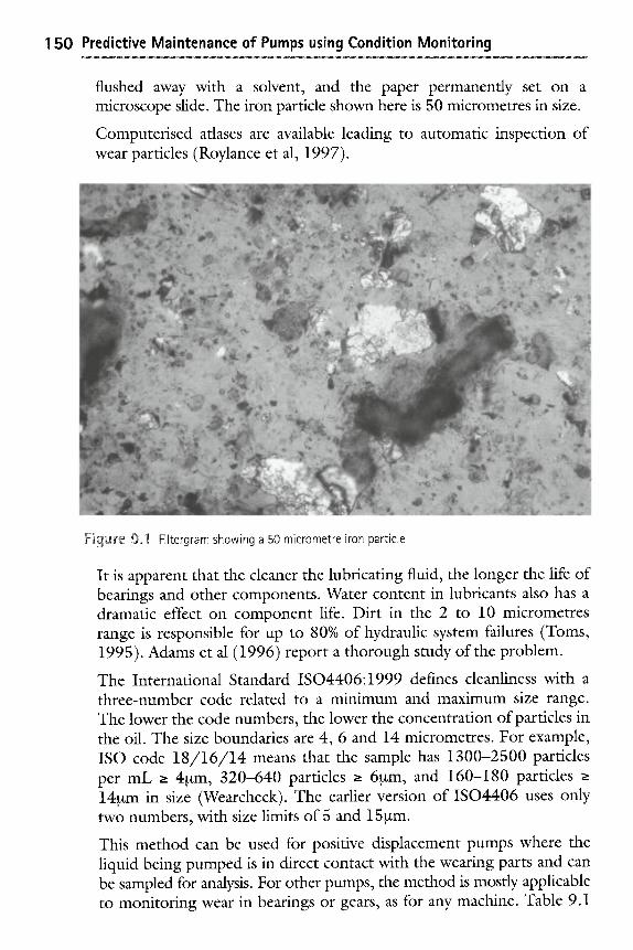
150 Predictive Maintenance of Pumps using Condition Monitoring ~ . . x ~ . - ~ . - ~ ~ - ~ - ~
flushed away with a solvent, and the paper permanently set on a microscope slide. The iron particle shown here is 50 micrometres in size.
Computerised atlases are available leading to automatic inspection of wear particles (Roylance et al, 1997).
Figure 9.~I Filtergram showing a 50 micrometre iron particle
It is apparent that the cleaner the lubricating fluid, the longer the life of beatings and other components. Water content in lubricants also has a dramatic effect on component life. Dirt in the 2 to 10 micrometres range is responsible for up to 80% of hydraulic system failures (Toms, 1995). Adams et al (1996) report a thorough study of the problem.
The International Standard ISO4406:1999 defines cleanliness with a three-number code related to a minimum and maximum size range. The lower the code numbers, the lower the concentration of particles in the oil. The size boundaries are 4, 6 and 14 micrometres. For example, ISO code 1 8 / 1 6 / 1 4 means that the sample has 1300-2500 particles per mL e 4~tm, 320-640 particles e 6~tm, and 160-180 particles 14~tm in size (Wearcheck). The earlier version of ISO4406 uses only two numbers, with size limits of 5 and 15~tm.
This method can be used for positive displacement pumps where the liquid being pumped is in direct contact with the wearing parts and can be sampled for analysis. For other pumps, the method is mostly applicable to monitoring wear in bearings or gears, as for any machine. Table 9.1
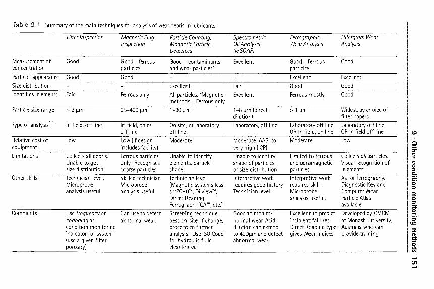
9 �9 Other condition monitoring m
ethods 151
-'3
C
C"
C./
C'-
.m t'O
E
c--
O
c'0
E
E
C~
t~
~Q
0 0 "~
0
Q
c-
~J
cJ X
I_U
4~
c-
,
c-
E._
~
O
O
--~
O
c (D
m
O
--~.~
C9
~
0 c
- c
- 0
E c--
~.;
c-
O
c X
U_
l
O
O
(D
c"
&
2
0 0
0 0
(.9
(.O
0 0 r,..O
ii
~J
c-
c~
X
~ ,,,
< c-
O
O
I u..
.~-
c-- r1
62
o E
"C'-"
~'1
.m
~
S ~ >
m i/I 0 E -m
0 i,_
u_
c-
~J
cJ X
u
J
>:.
y
2 I
N-
O
ii#
0 c-
_0
E "-I
A
E --I
O0
I
E ::I
0 O0
I
E
-I
0 0 'm'- I
0,I
E A
c c~
Q..
.c_ c_
1-.- O
O
O
~ ~
m
~ i.--
O
--
.c_ c_
~ c
O
O
>-~
~
m
O
~ ~
m
c~
4--
~-- c
- O
~
._O
.~
c-
4- O
O
O
_..1
O
O
O
c-- 4
-- 4
-- O
o
O
c-
O
m
.m
m
tl--- 4--
c 4--
m
O
.c_
O
c-
._m
m c O
�9 N- O
m
r
.--~ 0
4--' .m
"--- 0
o w
_. ~
0 ~.- e
- l._
o E
E
c- cu
.~1
('~
C
).
c-- ~
~._
o
4-,
--~
4-~
C
.~
Z3
c-
c-
".~
o m
-
c--
m
un
~
M
__~._m
~ .___
c- ---~
~g
n~
~ c--
O
u._
O
c.~
~-
c--
m
o .-~-
_0
---
~ II~
0 C
N
r~
zD
~
c-
O
.m E
._J
c-
~v~
O
---:
t4--
~ ~
O
~
~_.,, ~--Z b
>.
0
~--8>
" c
- "
:Z~ c"
N
cr~
:u_ -5
~o
~
m
n m
cJ
>
"m
,4-
0 m
~
"EE__ ,._ _
I--
c-"
o
~j
8~
o
.=- c'-
C
~_ ~.m
o~
~,,,<
S_
~J
"d o_~4
S_'5 ~-u c
- c
-
~,.->
-,:,
.
"
~
58
-E
~O
~o
~
O
Y~
c)
~-~ 5
m._
o
~-m
--~
o ~
~E
O
c-- c
-
c13
._
fE
6~,E~6
~,~ o
o "6~
~ ~
~._
..~
~
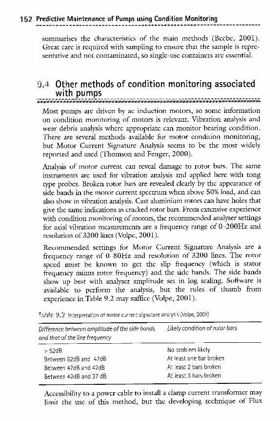
152 Predictive Maintenance of Pumps using Condition Monitoring
summarises the characteristics of the main methods (Beebe, 2001). Great care is required with sampling to ensure that the sample is repre- sentative and not contaminated, so single-use containers are essential.
9.4 Other methods of condition monitoring associated with pumps
Most pumps are driven by ac induction motors, so some information on condition monitoring of motors is relevant. Vibration analysis and wear debris analysis where appropriate can monitor bearing condition. There are several methods available for motor condition monitoring, but Motor Current Signature Analysis seems to be the most widely reported and used (Thomson and Fenger, 2000).
Analysis of motor current can reveal damage to rotor bars. The same instruments are used for vibration analysis and applied here with tong type probes. Broken rotor bars are revealed clearly by the appearance of side bands in the motor current spectrum when above 50% load, and can also show in vibration analysis. Cast aluminium rotors can have holes that give the same indications as cracked rotor bars. From extensive experience with condition monitoring of motors, the recommended analyser settings for axial vibration measurements are a frequency range of 0-200Hz and resolution of 3200 lines (Volpe, 2001).
Recommended settings for Motor Current Signature Analysis are a frequency range of 0-80Hz and resolution of 3200 lines. The rotor speed must be known to get the slip frequency (which is stator frequency minus rotor frequency) and the side bands. The side bands show up best with analyser amplitude set in log scaling. Software is available to perform the analysis, but the rules of thumb from experience in Table 9.2 may suffice (Volpe, 2001).
T ~ ~abte 9,,2 Interpretation of motor current signature analysis (Volpe, 2001)
Difference between amplitude of the side bands and that of the line frequency
Likely condition of rotor bar5
> 52dB Between 52dB and 47dB Between 47dB and 42dB
Between 42dB and 37 dB
No problem likely At least one bar broken
At least 2 bars broken At least 3 bars broken
Accessibility to a power cable to install a clamp current transformer may limit the use of this method, but the developing technique of Flux
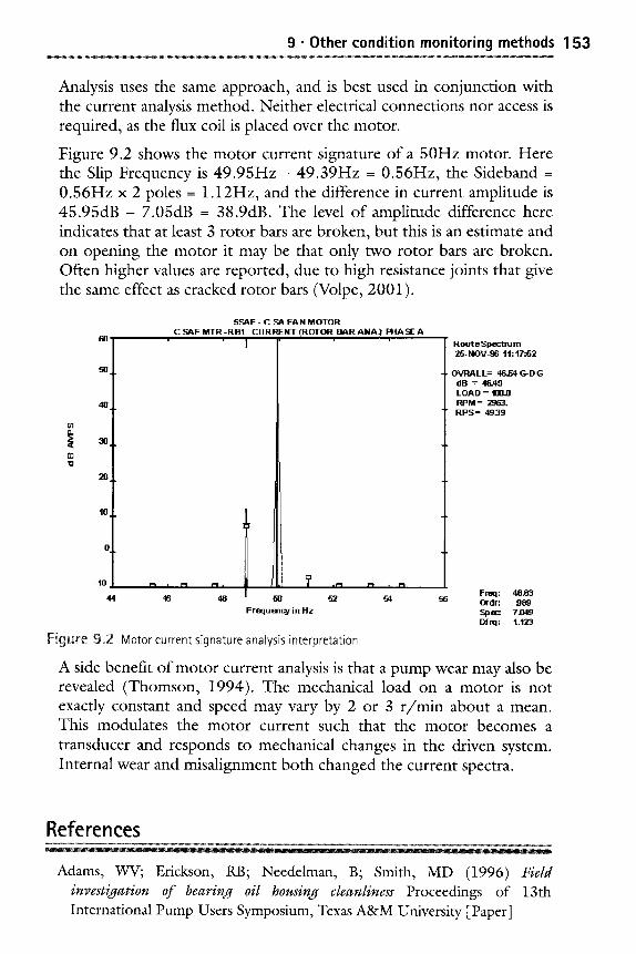
9 �9 Other condition monitoring methods 153
Analysis uses the same approach, and is best used in conjunction with the current analysis method. Neither electrical connections nor access is required, as the flux coil is placed over the motor.
Figure 9.2 shows the motor current signature of a 50Hz motor. Here the Slip Frequency is 4 9 . 9 5 H z - 49 .39Hz = 0.56Hz, the Sideband = 0 .56Hz x 2 poles = 1.12Hz, and the difference in current amplitude is 4 5 . 9 5 d B - 7.05dB = 38.9dB. The level of amplitude difference here indicates that at least 3 rotor bars are broken, but this is an estimate and on opening the motor it may be that only two rotor bars are broken. Often higher values are reported, due to high resistance joints that give the same effect as cracked rotor bars (Volpe, 2001).
10
-10 n .
44 46
5 S A F - C SA F A N M O T O R C SAF M T R - R B 1 C U R R E N T ( R O T O R B A R A N A , ~ P H A S I E A
f - i , I~i ,r i-t , I"1
48 50 52 54 56
F r e q u e n o l in Hz
Figure 9~ Motor current signature analysis interpretation
R o u t e S p e c t m m 25- NOV-~6 11 :17 :52
- O V R A L L = 4 6 - 6 4 G - D G dB = 4 6 4 9 L O A D = 150J) R P M = 29t]3,
" R P S = 4 9 3 9
l=req: 48.83 Ordr: .989 Spec: 7.049 Drrq: 1.123
A side benefit of motor current analysis is that a pump wear may also be revealed (Thomson, 1994). The mechanical load on a motor is not exactly constant and speed may vary by 2 or 3 r / m i n about a mean. This modulates the motor current such that the motor becomes a transducer and responds to mechanical changes in the driven system. Internal wear and misalignment both changed the current spectra.
References
Adams, WV; Erickson, RB; Needelman, B; Smith, MD (1996) Field investigation of bearing oil housing cleanliness Proceedings of 13th International Pump Users Symposium, Texas A&M University [Paper]
154 Predictive Maintenance of Pumps using Condition Monitoring
Addie, GR and Sellgren, A (1998) The effect of wear on the performance of centrifugal slurry pumps Proceedings of FEDSM '98:1998 ASME Fluids Engineering Division Summer Meeting, June, Washington [Paper]
Beebe, R (2001) Machine condition monitoring MCM Consultants, 2001 reprint [ Book]
Ding, GJ and Kuhnell, BT (1994) A cost effective combination of wear debris monitoring methods: direct reading Ferrograph trend analysis and filtergram microscopy Condition Monitoring 94, Pineridge Press, UK [Paper]
Fabeck, PH and Erickson, RB (1990) IS05199 standard addresses today's reliability requirements for chemical process pumps Proceedings of 7th International Pump Users Symposium, Texas A&M University [Paper]
ISO4406:1999 Hydraulic fluid power- fluids- Method for coding the level of contamination by solid particles [Standard]
Motor information: www.isr.gov.au/motors/index.html [Website]
NDT: www.asndt.com, www.aindt.com.au [Websites]
Roylance, BJ; Barraclough, T and Sperring, T (1997) Wear Particle A t l a s - a computerised window on wear and its underlying causes IMechE World Tribology Conference [Paper]
Roylance, B J and Hunt, TM (1999) The Wear Debris Analysis Handbook Coxmoor Machine and Systems Monitoring Series Coxmoor, Oxford [Book]
Thomson, WT (1994) On-line current monitoring to detect electrical and mechanical faults in three-phase induction motor drives Life management of power plants: IEE Conference publication No 401 (and similar paper in Condition Monitoring 94 Pineridge Press, UK) [Paper]
Thomson, WT and Fenger, M (2000) Industrial case studies of on-line CSA to diagnose problems in induction motor drives Proceedings of MARCON, Knoxville [Paper]
Toms, L (1995) Machinery oil analysis Coastal Skills Training, Virginia Beach. [Book]
Volpe, Clyde (2001) Electric motor diagnosis Handout notes [Unpublished]
www.wearcheck.co.za [Website]
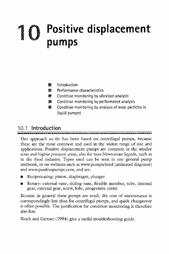
C) Positive displacement pumps
g Introduction m Performance characteristics Z Condition monitoring byvibration analysis
Condition monitoring by performance analysis J Condition monitoring by analysis of wear particles in
liquid pumped
I0.I Introduction
Our approach so far has been based on centrifugal pumps, because these are the most common and used in the widest range of size and applications. Positive displacement pumps are common in the smaller sizes and higher pressure areas, also for non-Newtonian liquids, such as in the food industry. Types used can be seen in any general pump textbook, or on websites such as www.pumpschool (animated disgrams) and www.positivepumps.com, and are:
�9 Reciprocating: piston, diaphragm, plunger.
�9 Rotary: external vane, sliding vane, flexible member, tube, internal gear, external gear, screw, lobe, progressive cavity.
Because in general these pumps are small, the cost of maintenance is correspondingly less than for centrifugal pumps, and quick changeover is often possible. The justification for condition monitoring is therefore also less.
Bloch and Geitner (1994) give a useful troubleshooting guide.
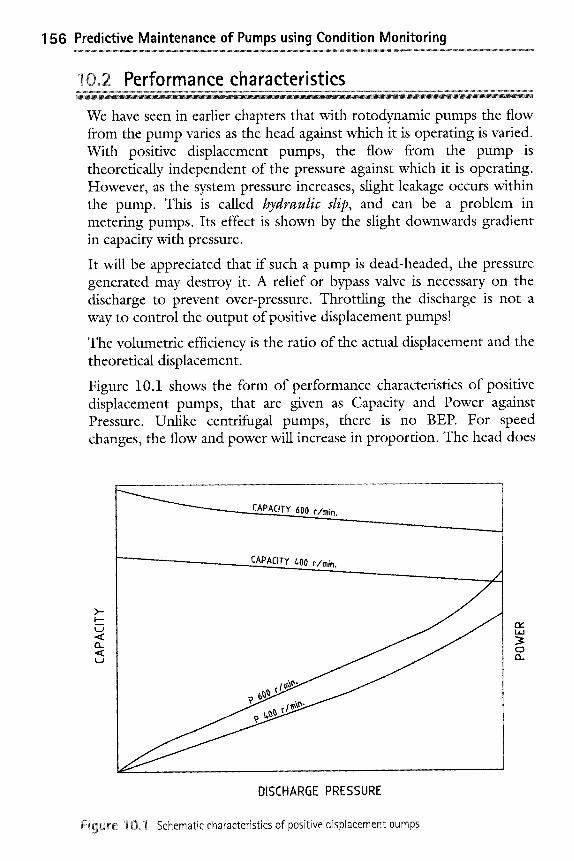
1 56 Predictive Maintenance of Pumps using Condition Monitoring
10.2 Performance characteristics
We have seen in earlier chapters that with rotodynamic pumps the flow from the pump varies as the head against which it is operating is varied. With positive displacement pumps, the flow from the pump is theoretically independent of the pressure against which it is operating. However, as the system pressure increases, slight leakage occurs within the pump. This is called hydraulic slip, and can be a problem in metering pumps. Its effect is shown by the slight downwards gradient in capacity with pressure.
It will be appreciated that if such a pump is dead-headed, the pressure generated may destroy it. A relief or bypass valve is necessary on the discharge to prevent over-pressure. Throttling the discharge is not a way to control the output of positive displacement pumps!
The volumetric efficiency is the ratio of the actual displacement and the theoretical displacement.
Figure 10.1 shows the form of performance characteristics of positive displacement pumps, that are given as Capacity and Power against Pressure. Unlike centrifugal pumps, there is no B EP. For speed changes, the flow and power will increase in proportion. The head does
>- l--
u .<( CI.
600
CAPACITY 400 r/rain.
DISCHARGE PRESSURE
Figu~'e 10ol Schematic characteristics of positive displacement pumps
s
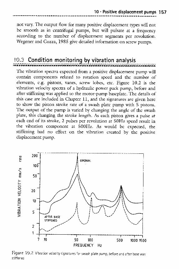
10 �9 Positive displacement pumps 1 5 7
not vary. The output flow for many positive displacement types will not be smooth as in centrifugal pumps, but will pulsate at a frequency according to the number of displacement segments per revolution. Wcgener and Cozza, 1985 give detailed information on screw pumps.
10.3 Condition monitoring by vibration analysis
The vibration spectra expected from a positive displacement pump will contain components related to rotation speed and the number of elements, e.g. pistons, vanes, screw lobes, etc. Figure 10.2 is the vibration velocity spectra of a hydraulic power pack pump, before and after stiffening was applied to the motor-pump baseplate. The details of this case are included in Chapter 11, and the signatures are given here to show the piston stroke rate of a swash plate pump with 5 pistons. The output of the pump is varied by changing the angle of the swash plate, this changing the stroke length. As each piston gives a pulse at each end of its stroke, 2 pulses per revolution at 50Hz speed result in the vibration component at 500Hz. As would be expected, the stiffening had no effect on the vibration created by the positive displacement pump.
I / I
E E
>-
kJ
c~ _J
z o
200~ t ORtGINAL 100 r ,
50-
20-
10-
I AFTER BASE ,/I ' \ ! ~,
I i ...................................... i .................. i ................................................ i ........................... i ..................
7 I0 50 i00 500 1000 1500 FREOUENCY Hz
Figure I0.~2 Vibration velocity signatures for swash plate pump, before and after base was stiffened
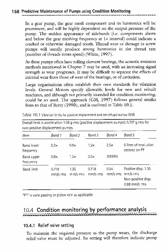
158 Predictive Maintenance of Pumps using Condition Monitoring
In a gear pump, the gear mesh component and its harmonics will be prominent, and will be highly dependent on the output pressure of the pump. The sudden appearance of sidebands (i.e. components above and below the gear meshing frequency at l x interval) could indicate a cracked or otherwise damaged tooth. Thread wear or damage in screw pumps will usually produce strong harmonics in the thread rate (number of threads times speed) (White, 1997).
As these pumps often have rolling element bearings, the acoustic emission methods mentioned in Chapter 7 may be used, with an increasing signal strength as wear progresses. It may be difficult to separate the effects of internal wear from those of wear of the bearings, or of cavitation.
Large organisations often establish their own standards for vibration levels. General Motors specify allowable levels for new and rebuilt machines, and although not primarily intended for condition monitoring, could be so used. The approach (GM, 1997) follows general similar lines to that of Berry (1990), and is outlined in Table 10.1.
Tabie 10o I Vibration limits for positive displacement and centrifugal pumps (GM)
Overall limit is acceleration 1.06 g rms (positive displacement pumps}; 0.707 g rms for non-positive displacement pumps.
Item Band I Band 2 Band 3 Band 4 Band 5
Band lower 0.3x 0.8x 1.2x 3.5x frequency
Band upper 0.8x 1.2x 3.5x 2000Hz frequency
5 lines of resolution centred on PF
Band limit 0.718 1.35 0.718 mm/srms mm/srms mm/srms
0.54 Positive disp: 1.35 mm/srms mm/s rms
Non-positive disp: 0.89 mm/s rms
"PF" is vane passing or piston rate as applicable
I0,4 Condition monitoring by performance analysis
10.4.1 Relief valve setting
To maintain the required pressure as the pump wears, the discharge relief valve must be adjusted. Its setting will therefore indicate pump
10. Positive displacement pumps 159
wear, if it is possible to observe and record it. In the case of variable speed pumps, as with centrifugal pumps, increased speed for standard duty points to internal wear.
10.4.2 Crankcase return flow
In piston type pumps, increased piston ring wear results in increased crankcase flow. On one pump type, a container had to be inserted by hand into the oil reservoir to collect this flow. To remove this potential health hazard and awkward access, a tee piece and two valves were arranged such that the flow could be diverted into a measuring container external to the reservoir.
10.4.4 Capacity tests
Capacity tests may be run on hydraulic pumps on mobile plant, if a flowmeter can be connected in the return line between the relief valve and the tank return. The flow rate is then measured at several pressures arranged by setting the relief valve. On heavy fuel oil installations, a quality volumetric flowmeter is often provided, and performance tests can be made.
10.4.5 The thermodynamic method
The thermodynamic method has been applied with some success (Balawender and Zielinski, 1991), provided the thermodynamic properties of the liquid are known or can be found (Witt, 1976 and 1979). As wear proceeds, running clearances increase. Internal leakage through clearances is a function of the clearance cubed. Thus a doubling of effective clearance means an eight-fold increase in internal leakage through it. The increased clearance results in a power loss, converted into heat (Tjorn and Dransfield, 1987).
The same approach and general precautions in temperature measure- ment apply as for centrifugal pumps given in Chapter 5. The isentropic temperature rise for an oil at 30degC is about 0.012K/MPa.
The higher the pump pressure, the greater the temperature rise for a given pump condition and efficiency. On a gear pump with 85% efficiency operating at 20MPa, temperature rise was 4K. At a pressure of 13 MPa, the temperature rise was 3K. When worn, at 20MPa, efficiency was 75% and temperature rise 6K.
Monitoring of pressure pulsation and check valve opening pressure shock are key elements (Martinez et al, 2000). Tests on diaphragm
160 Predictive Maintenance of Pumps using Condition Monitoring ~ _ _ . ~ . _ - . - - - . . . - - ~ ~ . - - < -_= . . . . . . .
pumps were performed to record dynamic pressure of an operating cycle. The traces over times of up to a second varied significantly with introduced faults.
Frequency analysis of the pump pressure tipple on a machine tool coolant pump showed the greatest component at rotational frequency (48Hz), with the next highest component of 74Hz related to oscillations of the relief valve, as it was absent when the valve was closed (Martin and Thorpe, 1998). Fanti and Basso (2000) have taken this further by applying Fourier Transform Triple Processing of the discharge pressure from gear pumps. A piezoelectric sensor was put into the fluid.
10.,5 Condition monitoring by analysis of wear particles in liquid pumped
For the types of positive displacement pumps where the fluid being pumped will collect wear particles, and a sample can be arranged, then analysis using one of the methods outlined in Chapter 9 could be used.
References
Balawende, A and Zielinski, M (1991) Overall and volumetric efficiency monitoring of hydraulic pumps and motors Condition Monitoring - Proceedings of 3rd International Conference, Elsevier. [Book]
Berry, JE (1990) Proven method for specifying spectral band alarm levels and frequencies using today's predictive maintenance software systems Technical Associates of Charlotte (4th Edition 2003) (www.technicalassociates.net) [Book]
Bloch, HP and Geitner, FK (1994) Practical machinery management for process plants Vol 2 "Machinery failure analysis and troubleshooting Gulf, 2nd Ed [Book]
Fanti, G and Basso, R (2000) A diagnostic technique for gear pump testing 13th International Congress on COMADEM, Society of Machinery Failure Prevention Technology, [Paper]
GM (1997) Vibration standard for the purchase of new and rebuilt machinery and equipment GM Specification V1.0-1997 [Company Standard]
Martin, KF and Thorpe, P (1998) Coolant system health monitoring and fault diagnosis via health parameters and fault dictionary in Davies A (Ed)
10 �9 Positive displacement pumps 161
Handbook of condition monitoring : techniques and methodology London, Chapman & Hall [Book]
Martinez, F; Philippin, M; Blanding, JM; Schlucker, E (2000) Dynamic monitoring for early failure diagnosis and modern techniques for design of positive displacement pumping systems Proceedings 17th International Pump Users Symposium Texas A&M University [Paper]
Tjong, KF and Dransfield, P (1987) On-line assessing of wear in hydraulic control systems: a review International Tribology Conference, Melbourne [Paper]
Wegener, J and Cozza, WE (1985) Screw pumps of one, two and three screw design
Proceedings of the 2nd International Pump Users Symposium, Texas A&M University [Paper]
White, Glenn (1997) Introduction to Machinery vibration DLI [Book]
Witt, K (1979) Verschillend gedrag van hydraulische en pneumatische energiedragers (Different behaviour of hydraulic and pneumatic energy carriers) Andrijftechniek, Nov [Paper] (In Dutch)
Witt, K (1976) Grondslagen voor het thermodynamisch meten an hydrostatische compnenten (Principles of thermodynamic measurement on hydrostatic components) Bedrijf & Techniek/Andrijftechniek, Nov [Paper] (In Dutch)
www.pumpschool.com/[Website]
www. mcnallyinstimte, com/home-htmlffFechnical_paper_index.html [Website]
Case studies in cond ition mon itori ng of pumps
These arc sourced from the author's experience and collected notes over some years, with many from conferences. Sources of many are unknown, but are appreciated. Data here shows that interpretation is often not clear, and the value of close correlation with as-found condition is emphasised for future diagnostics. Some pumps could fit into more than one category. These "war stories" are included to illustrate the application of condition monitoring, with the aim of inspiring pump condition monitoring practitioners.
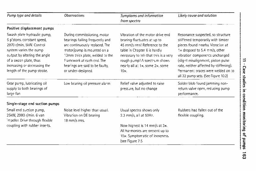
11 �9 Case studies in condition monitoring o
f pumps
163
0 �9 ..,...
0
,,,,,,4
0 �9 ...,...,
E 0 l:&
E
I/I
0 �9 ,.....,.
I, rl 4
~
I::::
E
E
O
~'-
~-- c
- O
~
JE)
c-
c13
m
..c
m
O
u O
~
'~'
o >
~
,.._
. ---
~ "~_._.o~
~ i.i -
'- m
o
E~
g~
c~
O
r
~ M
.- c13
g E
-~
"-- ,_
...o
= &
O
X
~ "--
4-'
~ I
>.
c-
~ >
~
�9 -~ E
~
0 0
> 0
~ ~
c-
.~_
~0
4_, i
.-- ~n
~
~<
x
~
~
E
-.,- ,--
,_, E
~
o
~-~
O
o'
~
c-
c13 c"}
r ~
"-- ~
c-
>-.
(u
c-
c-
~ ~.~
-~
�9 g
__
,:o_
o
�9 ~ m
>
, E
~
~
-~
�9 ~ ~
-~
.- ~
.~
~._
_o
N
e~
m
_o o
,-
" o =
~
~
~o
,'-
u ,-,
~
E
~
~
~
~
�9 ~
~~
_
~
&
E
O
"~
c-
.E
.E
g
._.-~
O
i -~
>
E
I1A
i./'1 .i ~._
s c
t~
~ O
~ E
E i1j
llj
CL
.i O
c- .m
i1J _
O
O
._1
n M
-- "~
O
c-
_ O
_
O
i
4--~ M
-- O
O
C-
Cl~
C'-
m
C-
O
-O
-~
IlJ rr"
~_
x ~
re Q_~
4--J I/1
----> ~
C-
0 c
- ~
~ O
O
E
~
-- ~
14
- E
T,.., ~
o O
~
-~
(13 ~t~
.~
s I'~
~ m
" ._c:
O
~
E
Z
N~
~
E
......2" c~
c-- c
- t'~
.I
..c
u_
l
c-" c-"
E
i O
i~_
G.r
>
c'- ~
~ "
~
E
.i o.-2_oo
Ill
E I~.
~ 1,4
c-- X
~
-
c-
'-,1 "~
..o c
do
-~
~
..O
~ (2
) "r-
"--
~ N
N
m
~ ~.r
C
" E
m
E
o
.i I,~
c
~
c,4
._
u
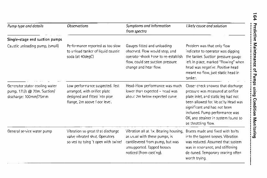
1 64 P
redictive Maintenance of Pum
ps using Condition M
onitoring
0 0
-...4
0 E
0 ~E
o . ..,,..
r E
cL
c
~ -~
c- c-
-s -o
.~
~_ &--~ ~
~ Q_
c- ~J
0 ~
-s "~
r c-
~_
co
~ O
.4
, .--
>.~
~
,T'~
~
O
~ u ~"
~._ ~.;
CO
~
O
_o
._~
~
.--~
~ ~
o
_.o
~
c ~
--~
0 ~
~ c--
on
..o
~ c-
O
0 ~
-- ~
o o o
m
~, o c-
g-~
,e
0 m
0 c-
~ o
o
i,['1 e'-
----,
.s
e-
c-
o c-
,m
~ ~
0
.m
(I~
.~=
6
g E
%
~ ~
..o
~ .
.~
~ E
~
o c-
~ ~
=~
o~
-~'-'
~.-
--~ ,u
- E
__ ~
=
,.- -,--
~, ~_ -8 ~ o
0 ~
co ~
d r~
~"~
r'~ _
o
~ ._
c-
~ ,
-'d
E'g
#
X
~ _0
..0
~J I---
._o_
~_
~_
o
-~
~q cj
c- O
~
"-- O
E.S
N
--~ ~
- ~
E
4-~ c O
OoE
c;
I'~
o o c- r~
(D
Q--c~
E
c-
o
~-~
%
~.u
"~
~-~
~
x ~
E
~- >
"
~ ~
.
#~
~
~_ ~
4--~ CO
o~ c
-
s
c E
~
o
�9 ~
Q-
~ 121.. 4
-I x
~ E
,-,
N
__ ~
_o
"d
E
g -~
~ o----
-"-'L-- iz~
~-~ c-
O
m,
~.j r
--5o
~
-~ Q
.. c
O go
%
-,~
o ~
~.
~_S
>- >
"o
> >
~ ~
o
E :C5
r > ~J
r C
~J
co
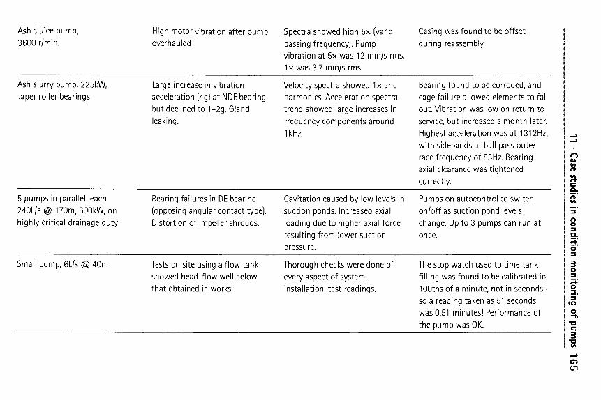
11 �9 Case studies in condition monitoring o
f pumps 165
b~
0 (u
...o
0
-o._~ c"
._0
=
E
0 b9
b~l
Ct~ Ct~
c'- c m
(..)
E c
- I,~
x E
c- I:::
~ X
E ~
g_
~E
..
0 un ~
c-
C~
l:~
0 un
~'~
~
c~
co
._
X
E IU
c-
O
._0
0 -0
0
7-
0
E
.~
E
un 0
c-
0 un
(.0
0 c
- ~
C",,I
~.-
~ ~
-- "r"
"~
g ~--
~ ~
~ c--
0
.7
~ .~
0
~ ~
c-
c- c-
O -~
~_~
g-8
~ ~
_
~_ ~
= -
-~
"o
o-
>:~
~ c~
~'
~-
~
~- ~
�9 "s ~
~
8-a ,',',
~ o
~ ~
'.~
~
-• ~
c-
• 0
-0
c-
~-
m
~.J
~ ~
- 0
~-
E~
N
o
~~
~
~-
~_. c'-
CJ-
--r"
c--
c- _
0
c- O
G
~
_~z~
.c_ -~-
~-~ 0
~ ~
"~ .E
c-
eft_ "r-"
..0
>-~
0 ~
-6~
~_
~ o
E
8 g
~- 0
CO
m
~
c-- ~
c-" ~--
c--
c-
~ o
~ -0
X
I,/'1
U
c-
~ 0
0 ~
~-
c~_-c~ o7
~j
~ o
~-'=
~=
,.---k
._
~ --3
S
8~
8 -'
E
~..
07
-~
-7
C
4
-- ~
C~
12)
~_m
Cn
C
c'-
0 ~
..
..
-~
~:~
.--
P~
m
E .~.~
>.
I
~ o
~
~ Cl3
.p_,o ~
~6 G
,
c-
O
c-
~.-
~ ~
~_
~
~-N
~
NN
"--
C)
0
4-- 0 IU
c-
E-.E
IU
4--
I/1 ~
o ~
c-" C
:I_ .~
0 >
.--~
0
_.o o
~,,,
0
._
c-
g -g_o 0
~ o
~
~LI c
- ._C
E 0 @
__1 (.0
o7_ E
E I,/'l
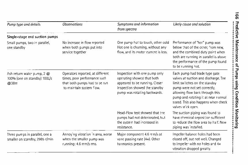
166 P
redictive Maintenance
of Pumps using C
ondition Monitoring
~-
~.
-
.-.- __ _ ~
.~
0 .!...i
0
�9 ...... ......I
0 , .....
E
0 0 �9 ......
l:b
"0 E
~o
-,
~- ._
"~ -~
r
-o
"--
=
~'~ ~.~
~
Iu
0
.-~~
~ ~
~~ N
o ,,_..z
E~
,.,
~~
==,_
r ~
c-
0 ~c-
O
~-
~.~ M
b~
r
-~
.--
c-
O
~ ~_
~ ~
O
o-~
~
~ O
~ ._
--~
~ O
c- O
O
O
"r-
~__.
~s
Z
c ~
_
Z~
~ E
~
�9 --
~
~J
(U
m
E
~J
C
--"
,m
'- c "~
0
6
E-~
,E
~'-
H--"~ E
..c ~
Z
~ g
~ ~
c~ o
-~ ,.,,_:
�9 ~
r
r +-~
.__
>-
~
~_ r
-o
~
-~
-o
~-
~
r
0
c-
_o
i/~ ~
~.~ -~
~/~ M-
0
-= o
o-~
_~
'-~
o ~_
_, ~:
~_
~.
o
~- .~
.,:, ,-
~--~
.-~-5
5
"~:
-~ ~;
~-~
'~
-~__ =
~_~ ~-
,,, >
._
~_
~ ~
_ ~
> ~
_ _~
o
-~_
4~
~-_g
oO
~
-,:"-,.~g
~ o
~
~
--
0 c
~
.--
O_
I
~-~
4-,
~_
-i• c"-
c-
:z:3
-0 4
-1~
C
- s
s ~
dE
2:E
E
m
~- ~
~'~
~ O
"--
k ~
.E
o~
_~
~
O
C,,l
O
._o
�9 m
-1~
c-
s
r c
-
O
c-
(u
c-
::3
O
"-" E
c-
O
co
.2o@
-~o
~
~ ~
".~ o
O
._o
E
~o
- s
..c
o
~D
X
~ ej
c
~-- G
.J
tj r
c-
~,_ c'~
O
o ~
E
O
c-
"~E
_
~
E
E
~
-~.
c-
~-c-
O
I.O
co
O'b
._O
c-
c-
"-- s i.fl
O
(U
{U
=
~- E
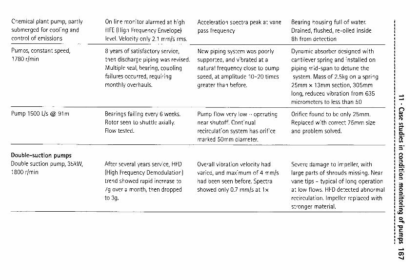
11 �9 Case studies in condition
monitoring
of pum
ps 167
~
~ ~ ~
,~
~ -~.~,,~.~
x-..~,,~..~
t'~
.m
o=5
-5 .b
~ c--
c-
�9 r--.c_ ~_
c--
>
c~
4~
~- 6
.O
m
~ E
< ~ o
...~ ~
E
w
-~
c- >
.
O
c-- ~
.
m
>
T Ca
>,
c'}
c'} c-
"~
O
c o
"g- s E
~
J
E~
c
- c'-
~ o
.~ E
E~
"~
~
~ ,.1_,1
-
c-
c-
O'~
M-~
g~-~og c
-
,,, --
~ ~
g2:
~
.~
~-~
,.. o
E'~
o
o '-'
~ E
-'~ ~
I/3
"~:--~
~
E
'- o
�9 ~_~
~
c~ P_, ~
.. ~
,.,, _ o ~
:
>.
E
ca -~
m
E
0
~ o
_'4
~
O~
oo
i./'1
~ ~
I c~
~
~ 0
0 ,--
.~_
N
,.,- %
~
Z
m
E
m
E~
75
~= 8:~
>
.. -~
c-
~j
~_ "~_
"r- ~-
~ "~..
~ -~-
",
O
-~
~
0
t~
E
C~
u E
c~
--~
p~
N
E~'~
E
E
NE
L~
C-
~ O
~ O
>
C"
m
"3
~ O
C~
m
.m
~,r
~ O
,92
-s-
.E
E
E
m
E
m
c--
i/i >:.
(U
u
CD
X
s
>"
CU
m
c-
c-
O
.m
4-1
~n
cu
~
C--
~._
O
m
r~
~___
E
Ob
I./'l
O
O E
cl
m
= o
E~
(U
.
..
.
=z
%
8 ~
�9 O
m
~
~-
-
~ ~
E~
~~
-- �9 --
-o
-~
o o-~
~_ 0a
~ "
~_-r-
_ o
~w
- >
.
~.~
o-~
E
~ E
~
x
o E
~
> E
.9
= c
d
E
"sg~
o
~ m
m
~
O
>
~ m
r'h
c-
0 L.L_
0 ~
_ ~3
I/I
Cb
.~
~..
m
123 s
c-
~"
c c
o"
>
l; 0
c~
~_. :-r=
ca <
~~
~o
LO
E
O
t-- "
gO
= u
c- "-3
I V
'I "~-"
.~
._o
0
0 0
oo
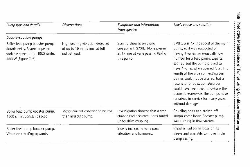
168 P
redictive Maintenance o
f Pum
ps using Condition M
onitoring
0
0
a<
0
,....
~t
E
e ~
~E
0
uD
C~
c~
E
c-
~ ~
~ �9 --
c-- .--
>
(~
~--
E ~
S o
~5
o
,_
~-
~-
E
~ o
-o
"' o
>-'Z
9
~S
-~
=E
-u
S
d_
&
'-
~n
Q-
._
._~ ~
~- ~
~-5
o
.~ ~
.=_
~
o O
_o
~,,,._o
s >
~_
_~
,.
_
>
0 4.-,
4-,
c-
O
X t,.O
(U
IU
1:~
c
- c
- c
-
o~
~
-~
Ni
o._ O
"T
" ~
J
c15
c-
c-
~._
~ g
~
~._ =:5
Q-O
~
'~
4-,
q- ci5
_O
G~
E
~
O
o--
co
O
{--:
E,_
-E
~
O
O._
O
0 "--
0 ~
0
,--~
...0
C-
4--' G
3
N
N
-E o.- ~ m
~
,po o
gg
o
1::13 "-O
>
E
-~ 8
~
c-
O
~--
o .E
8 ~
~ g
M--
r I~
0 "m
O
_
C-
0 C
;
0
-~
�9
~
co
>
c-
-~--
~Z
g
0 >
g &
~.-- C
O
o ~_
E
~_
"o
u'~
u'l
O
4.-., O
c--
-o
c-
~ E
t4
-- ~ 0
--
0
0 L
O
Iu
c-
i/~
c-
c-
>
0 0 E
gs
--
C
j
e ~
E
~ -~
~
CO
{:L
cu .~
c
- c
- G
I O
> E
co
"-o
GJ
c-
b c-
c-
"~. o
O
_o
d_ E (u
co
O
O
_o
c-
E :-5
4.~
~ g
14_
(U
Gi
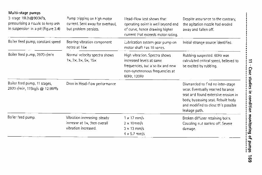
11 �9 Case studies in condition monitoring o
f pumps
16
9
r --~
o o
~ c~
o ~ ~
o c'-
O
c'- ~
r ~
c O
~ ~..
i./1 --
.r E
o -~
~ ~
o
~
--r- o
o ~
0 ~
-
0 Iu
E
> 0
o ~
~
~S
E
O_
~'I
--
"~__
. _0
"~
"~
0 O_
Q.;
~-
o ~_,____.
n
,.,,,~ ._. -~
"~_
t~
Cr)
~ m
.- g
g
~
NA
~
_.E
-d
c O
c~
r
._
c-
c O
Q
E
E
c O
c~
__.1
c O
E
O
c O
c (D
r c~
r O
E
O
121
O
Q.;
> u~
Q
.;
N
-r -~
-
�9 r" ~
.
.c_ ~
.~
.~
~ X
O
r ~
~ ~
X
~
~ ~
o ~
crl
_~
-~~
~
~
._
~.~
_
oo
O
c~
g_x
._c E
O o7.
E
"3
4--
O
r~
r �9 --
>._
_~
~
.~
c -~
_
o
Q..;
~ .o
o .~
,~_
_~
.;--,
o
O
_c
-~
r~"
~
g g
~
O
L.L.I c--
._~
~
g e
~2
N
~
Q.;
c.; c
-
E
O
,4-
Q~
c~
O
(.~ Q
.; "-r
c~
O
n
E
L~
0 -- O
C~
rn
c',,I
Q.;
bq
"~ o
Q.;
~._ CJ
~_o
0
E
X X
X X
O
~ x"
~ C
J ~
C.J
c-
~ c
-
CO
"4
~
CO
(U
C
O
_O
C
J _
O
E
c~
-o
G.J
O
c~3
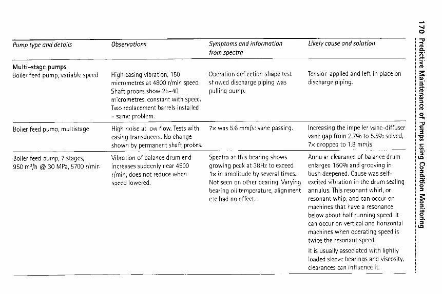
170 P
redictive Maintenance
of Pumps using C
ondition M
onitoring
E 0 E
E
o c
-o
m
ch
cxI
c-- 0
co
-~
_c:
b~3
C-
C'-
Oh
--o
~ E
g~
5-"
~ ~
.c_
tm
~.
o =
~
"~
00 0 ~
-'& b' -2: F~ ,
"0
o_
b,3
._o
.m
Ill
s ~
. >
E
o- ~_E
I 4-
_.= 0
r
~ >
.b o
> ud
~
o E
~8-
~x
c~
c-
>
b4
E
E
~D
ud
X
P~
u4 c
- ~./
.4=,
_0
-~~
@~
~
:n= ~
m
07
s
4.-a
4--,
E
E
E3
c'~
"-0
i.._
0
o7
n
>v. E
"- -,-,
m
._
.4._, ~
>..._
~
- -
"~
c-
-~ =~
~ 8 o ~
o-~
o ~ ~
-~ -~
-- ~
-~
o ~
~-o
~ F:
~ ~
_~ o
~ c_ca
c-._
~
~~
~~g
0 l'~
m
4-a
c"
s
~ (_~
0 c
- c~
~
_
"4~
0
--
~'-
~ 0
(1.; .~
o
~
~
>.ca
=~
~-
~ ~
~~
c
- ~
c"
~
-'~
c-
c-
~ 0
c-
~.t
"~
~.~ s
0a ..o
ca c~
~._ ca
~ --~-~ ~
"-O
4-a c
- c-- G
.;
._~
�9 ~__. ~.~
z- 2
4- r
E
c"
0 c
- =~
= g
==
K a
x "6
~ ~
k/3
07
,~
Z
..0
~ ..c
~.j c--
--~
>-~
c-
~~
_o
~_
~_
c-
E
un
-O 0
cy
l I'~
ci3
L~
4.-1
m"
I'~
r'l
~~
"o
~ E
~
0
rn
~
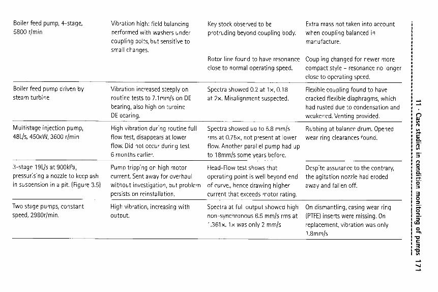
11 �9 Case studies in condition m
on
itorin
g
of pum
ps 171
"-'s 0
0
o E
0
o--
~
~- ~-
o o
~
4-a _
0
r
0 ~
~ m
~
-_~-- ~
c-- ~
~r~_. ~
m
-7
4-,
0
X
w
~ E
rj ca
-~
"-~
0
0 0
c'- ~_.
~ 0
"~
-" E
0 ~
~ c
-
.~
c-
�9 -- .0
. 0
-.i.,.-,
.~
o ~
O7
r
O
c-
"-~
~g
~
._O
c-
r R
:D
I/1 1./1
._~ ~
~ 4
-- ..~
�9
. ~--
_C::
.~
m"
~
o E
~ ~
.~
t,M
I/1
4 E r
..~
c-
iu
~u E
4---
�9 "~
O
O
C
O
r'~
~..c
c ~
o
c- m
- ~
-d
c'- IU
_
~
~ E
8 M
"O
I/1
C-
�9 ~
~--
d ~
X
~
('N
c-
d E
W c-
c-
>"
O
:.~
~o
~
~:~
o
._o ~
~ ~
c-- c--
._O
c-
r
.m E
E
1/1
"I:D
c-
O
-d
E~ c
-s
O
~.- ;,4..-
c-
c-
_o
r O
7
O7
c
-
_O
~,-
...O
E
-- _c:
~j
~~
>
.
~<
~ E
~
o
m
4--
~
~_
o
~
~-
o
~ {_
~ ~
-~
f: 5
~
E
o
--r ~___.
~____ ~
o7. E
.E
go
0 8
~-
c-
0 c
-
c-
O
._O7
~ ~
o
O7
0
~ .~
- E
o _~
~ I,/'1
.m
IU
~~
~
0 0
U
E
"-'s ~
- ~
0
C
m
o ~
._~
c-
I~
~o
~
O
-~
1/1 r
~--
~"
o7
o
c~
c
-
- E
o
tJ
~--
o~
-~
~-
~ E
c-
I/1
~ E E
~c
d_
_
~
O
O
I,/'1 m
c-
r
c-
X
._C
.m
.E
I/1 G
~
tj
.E
c"
.o
_O
"-s c
- 0
7
"~
7-
O
c-
c-
O
tj
O
00
Cl~
r
I/1 "O
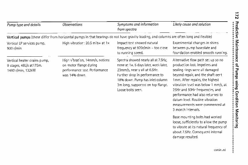
17
2
Pred
ictive M
ain
ten
an
ce
o
f Pu
mp
s usin
g C
on
ditio
n
Mo
nito
ring
O
, ,..... .4..,o
O
.....1
O
, .,...
E
aK
ES
O E
c-
c-
E
-'~
~
�9 -- s
�9 ~
~_
~
~- ~
,~
c-
E _m
_o 0
__
0
-o
r 0
c-
m_
~.~-
o o~O
-~
~~
~
.~
c-
12)
m
•
c- ~
�9 u- ~-~
~ +
_.~ _._m_ m
~ m
d
c- ~
4
O
c- c-
O
._~ �9 c'-
"T"
O
c-
O
4--
4--
~5
d
N
~
~ ~,
o ~
~"
o ~
E
o
c-
c-
-0
~ I1#
II#
c-
c-
c-
~ -
~ ~
~ =
-~
~ ~
o =
o.
5 o
=-~
~
-
= o
,,,~,.,
g ~
_ =
_9 =
-- ~
.-~
-~ ~
%
",~
".~
~ .-~
O
::3
~-~
.- o
~ ~
"5 o
E
._
~ _~
r
LO
C~
0 C-
(13 -
~ c
- ~b~
-~_ .-
c ~
~ ~
o
~ o
-- ~
.- c
- -0
~'-
~ -~
~o ~-- o
_o
~-
~ 0
Q_
o
0o
~
00
E
o
c-
(~1
I_L
~
.-- 0
o
__1
-o
�9 .~
c.- s
o E
i,_
~ O
"{- Iu
c-
">
O
,,-- c-
O
"-- c
-
.-~c
~
~ I
o o_~
E
-o
r C
~l
c- _
E
O
O'b
,--
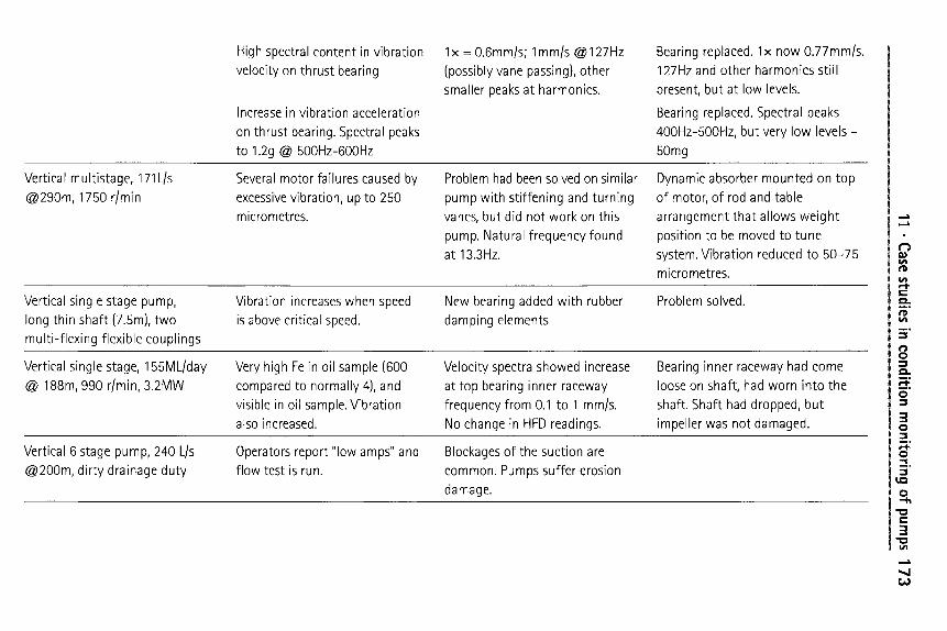
11 �9 Case studies in condition monitoring o
f pumps 173
t~
E
__m
E--
~
~
d 8
~-~
o o
-~
x ~S
__~
" ~
_o
c N
c
.~_ N
~n
~J
C',I
~
~J
0 0
N
7-
O4
(U
@ o
E O
E
.m
c-
E
c~
i
x &
E
c-
c-
~
o o
--~
.i
I
c-
._
-~___ r~
cA
J
_
G:~
~
I~
0
(u
_o
~_. .~
--~
"- ~
N
�9 ~ c
" c
- --~
.I
~
~--
-- ~,
g g
o
O
r'~
c-
O
g --~
o
g ~,
~-
~
u ~
E
"-' >
"~
~-~
b
c~ ~ ~
i c-
.i c
�9 ~ S
~
=
0
'-~
0 ~..
c"
�9 ~ ~
.5 5s
~ ~
c"
t,._
.~
~..
>,.
_.O
"O
O
~J
1.13 y
~
8 o
uq
Q
-
~ o (.~
o'~
-~.~
E
O
F-. ,i
.E
&E
~
o
".~
L.O
r-.. E
4-,
(U
> O
E
_o
O
!,._ (u
_
o
._o
c-
4-1
"-~
c-
�9 -~
~
j
E
C13 i:~
..O
"~
Z
"~
"O
(U
i/i
c-
8
g ~
._o
cl~
.I &
8
"~
c-
�9 .~
cD
n 4
-'
8o
~
0
.I b~
E
>._o
g g
g "-~
C
"
~ c
" O
~_@
_~
E_
_~
o ~
E
o ~
z X
~.E
>'o~ -~
CA
~
m
>-
L~
,
�9 --- C
O
~ O
G)
c-
._o
c ~
._o ~
~ E
~ E
~
c-
% E
c~
O
i = o ~
o ~--
i/'1 >.
0
m
~t- -o
c~
~A
c
~.j
"-O
~2
n
>-
t~
"o
N@
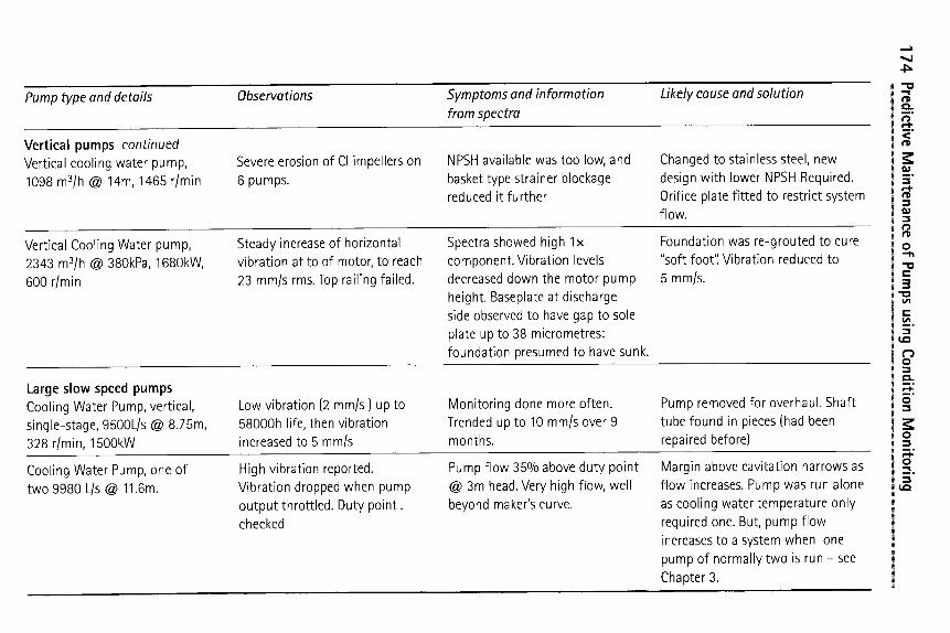
174 Predictive M
aintenance of Pumps using C
ondition Monitoring
..... ...~
..~
2 E E
�9 ,..,..
�9 .,.,.,
E
I:k
E
E
-d~
c- cr
-~
~ ~
-'o
-~
~
o c-
~ ~
co
c-
~ ~
.-~
~
c-
m g
o b
~.E b
c-
O
E 0 c 0
.m
0 b ~ I21..
~ E
.E
~_
(,D
&~,--
NN
~
c.; 0
0
::5 -,i
-0
0
0 co
o~
0
g~
E
u_..-m
m E
-6 ~
Q.-
~ 0
>
x~
R2
~E
~=
i
"- ~
E
:-c3 ~
E
~o
~.>
o~
c'-"
co
4-1
m
-~
�9 g
t~ ~
~ 5
-gN
b
~
g._ ~
_~
o
~ E
b
~2
Q
- o
~ "~
"o
_~
~
-c:~
c
- "~
Q
_~
_
o
. �9 =
~
.E
"6"6o
0 ~
-~E
m
E
(~
~._
N
.x2_ m
m
> o
4
d 0
~d
:g@
%
~
~o
:N
m
~
c',l (D
w--
....2" ~
j
> ,---"
0 ~
~ 0
~ E
E
E
~
0
gs
c- --~
0
0 ~ 0
.m
E
._o ~
E
~ "~E
0
.~o
~
.....1 L
~
._
E-
~
~
00
a_
~
E
~- OU 0
r
_ Lf)
~ 9
E
~.c_
~
-.~.
..~ r~
~ c0
t~
i1j
o c--
i o
c ~
o
~-~
Z~
~-
co E
o ~
~, _
o
~ o~
o
~ c-
c6
~ ~
~._
~c~
c-
m
-~
0 ~
--
~-gr
0 ~
~N
E
"o
~ E
c--
m
._o
c-)
E
.,_., �9 "~
c
-
o._
" 5 >
.
-o
r'~
gg
-~
-~-~
s
I>
o
u
M--
O
t-
oE
o
_(.D
E
,--
2 Cl3
.~1
~o
00
.~
O~
O
O
8~
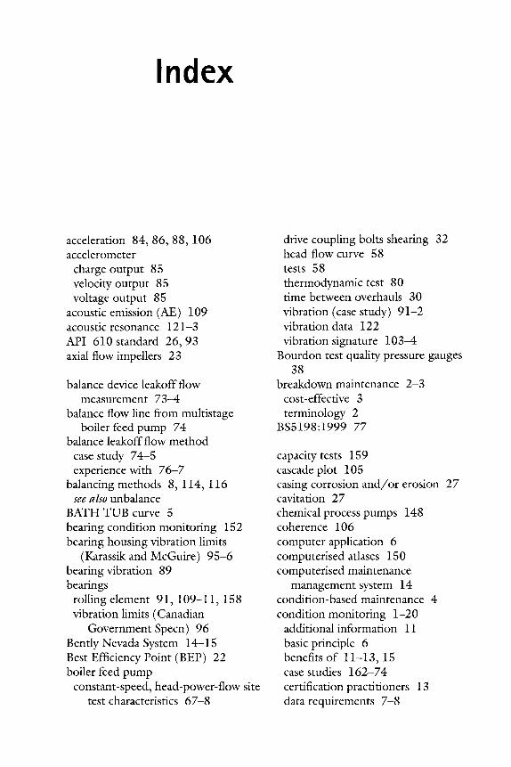
Index
acceleration 84, 86, 88,106 accelerometer
charge output 85 velocity output 85 voltage output 85
acoustic emission (AE) 109 acoustic resonance 121-3 API 610 standard 26, 93 axial flow impellers 23
balance device leakoff flow measurement 73-4
balance flow line from multistage boiler feed pump 74
balance leakoff flow method case study 74-5 experience with 76-7
balancing methods 8, 114, 116 see also unbalance
BATH TUB curve 5 bearing condition monitoring 152 bearing housing vibration limits
(Karassik and McGuire) 95-6 beating vibration 89 beatings
rolling element 91 ,109-11 ,158 vibration limits (Canadian
Government Specn) 96 Bently Nevada System 14-15 Best Efficiency Point (BEP) 22 boiler feed pump
constant-speed, head-power-flow site test characteristics 67-8
drive coupling bolts sheafing 32 head-flow curve 58 tests 58 thermodynamic test 80 time between overhauls 30 vibration (case study) 91-2 vibration data 122 vibration signature 103-4
Bourdon test quality pressure gauges 38
breakdown maintenance 2-3 cost-effective 3 terminology 2
BS5198:1999 77
capacity tests 159 cascade plot 105 casing corrosion and/or erosion 27 cavitation 27 chemical process pumps 148 coherence 106 computer application 6 computerised atlases 150 computerised maintenance
management system 14 condition-based maintenance 4 condition monitoring 1-20
additional information 11 basic principle 6 benefits of 11-13, 15 case studies 162-74 certification practitioners 13 data requirements 7-8
176 Index
condition monitoring (c0ntinued) definition 5-6 experience with pumps 12-13 methods 146-54 organisational arrangements 13-14 positive displacement pumps
157-60 seal-less pumps 143-4 shaft seals 142-3 techniques 7-11 test procedure, example 69-71 trending 7
constant bandwidth filtering 104 constant percentage bandwidth filters
102 constant-speed boiler feed pump,
head-power-flow site test characteristics 67-8
contact transducers 85 contaminants in process fluids 9 corrosion allowance 148 cost per month calculation 64-5 crankcase return flow 159 critical speed 108 cross-correlation 106 cutdown impeller, power savings with
138-40, 142
damping 108, 126 data fusion systems 8 decision support systems 14, 107 degradation see performance demodulation 109 design out maintenance 4 diagnosis of machine condition and
faults 110-23 direct metal-metal path 109 displacement 84, 86, 88-9, 106 double-suction pumps, case studies
168 drive coupling bolts shearing, case
study 32 duty point test, pumps in
combinations 56-7 dye dilution 46
economic wearout 3 efficiency 21-3
and internal wear 28-9 calculation 47-8 deterioration 29 improvement measures 135-6
efficiency, determination from test results 78-9
electrical plant testing 11 electricity consumption 63 electronic data collector/analysers
106 electronic tachometers 47 enthalpy-entropy chart of steam/water
properties 78 enveloping 109 erosion, impellers 24, 27 Europump guidelines 93-5 exciting force 108 expert system 107
failure definition 3 statistics 131
Fast Fourier transform (FFT) algorithm 103-4 analyser 108 averaging 105
filters 102-5 fixed time preventive maintenance 3 flow 21-3, 50
indirect measurement (case study) 53-4
flow metering 41-6 low flow protection 42
flow rate 31 flux analysis 152-3 forcing frequency 108 free discharge outflow, co-ordinates of
46 frequency analysis 101, 160 frequency bands 127-9 frequency range 106 friction head (kQ 2) 48-50 full head-flow test 57
economic failure 3 gauge pressure 37
Index 177
gear meshing frequency 107 gear pumps 158 gearing vibration 91
head 21-3, 37, 50, 138, 141 comparison with works test
measurements 40-1 head-flow curve 57, 65,140
boiler feed pump 58 head-flow data, finding optimum time
for overhaul from 63-4 head-flow measurement 56 head-flow performance, bypassing of
balance valve seat showing reduction in 77
head-flow power tests 56 head-flow test at duty point 57-9 head-power characteristics 80-1 head-power-flow
in new condition, with test points showing internal wear 62
in new state 66 variable-speed pump 66
head-power-flow site test characteristics 62
constant-speed boiler feed pump 67-8
high-speed camera 147 hydraulic inefficiency 48 hydraulic unbalance 117 Hydraulics Institute 28 Hydraulics Institute guidelines on
vibration 93-5
impact damage 27 impeller
axial flow 23 blockage 27 cutdown 138-40, 142 damage 98 erosion 24, 27 expected frequencies of vibration
with various combinations of numbers of vanes 120-1
mixed flow 23 radial 23 severe shroud damage 114
smaller than expected (case study) 33
specific speed values 23 see also v a n e
impeller diameter calculation 137-42
impeller diameter factor 31 impeller trimming
large size p u m p - 1320kW 140-2 medium size p u m p - 132kW
136-40 induction motor, speed measurement
46-7 infant mortality 4 infrared thermal imaging 9, 147 intermittent operation 61-2 internal wear see wear International Foundation for Research
in Maintenance (IFIRM) 4 ISO3945:1977 90 ISO4406:1999 150 ISO5167 42-3 ISO5199 26 ISO13380 10 ISO13881 6 ISO 18436 13 ISO 180816 92
key performance indicators (KPIs) 1-2
leakage internal 25 internal seal 27
linear amplitude scaling 102 linear frequency scaling 104 logarithmic frequency scale 102 logarithmic scaling 102 looseness 118 lubricants
wear debris in 148-52 wear particles in 9
machine life cycle 4-5 early life 4-5 useful life 5 wearout 5
178 Index ~..~ ~ , ~ . ~ : . . . . . . . .
maintainability 3 maintenance
as reliability function 1 basic types 2-4 fixed time or duty basis 3 philosophy 1 prioritisation 63 purpose 1-2
maintenance cost relative to vibration (BuscareUo) 95
maintenance errors 27-8 maintenance management,
engineering component 13-14 maintenance management system 5 management decision 4 mechanical tachometer 47 mechanical unbalance 114-17 misalignment 106, 118
case study 97 mixed flow impellers 23 modal response circles 109 Mollier chart 78 motor current analysis 152 motor current signature analysis
152-3 multi-stage pumps 29, 73
case studies 169-71
natural frequency 108 nodular growths 26 noise and vibration 84 non-destructive testing (NDT) 9,
147-8 non-synchronous characteristic
frequencies 109 Nyquist diagrams 109
on-line monitoring systems 8 operating point 48 opportunity maintenance 3-4 optical boroscope 146 optical fibrescope 147 orifice plate 41-2 overhaul calculation 60-6 overhaul optimum time calculation
from head-flow data 63-4 overhaul time optimisation 56-71
parameter change 10 peak-hold averaging 105 percentage reduction in performance
30 performance 21-34
basic equation 21, 47-8 basic quantifies 21 degradation, stages of 111 degradation with time 30-1 fundamental terms and units 22 percentage reduction in 30
performance analysis 56-71 applications 36 data requirements 35-6 methods 72-82 positive displacement pumps
158-60 performance characteristics 21-3
effect of internal wear on 26 positive displacement pumps 156
performance monitoring and analysis 9 performance shortfall, case studies
32-3 permanent monitoring 127-31 perturbation 109 phase analysis 107-8 phase angle 107-8 piston type pumps 159 pitot tube devices 42-4 positive displacement pumps 150,
155-61 case studies 163 condition monitoring 157-60 performance analysis 158-60 performance characteristics 156 vibration analysis 157-8 vibration limits for 158 wear particles analysis 160
post-mortem 14 power 21-3 power absorbed by pump 47 power consumption, effect of internal
wear 28 power-flow curve 136, 140 power measurement 47 power savings with cutdown impeller
138-40, 142

Index 179
pressure measurement 37-41, 159-60
instruments for 38-9 pressure vessel head (PVH) 48 preventive maintenance 3-4 process fluids, contaminants in 9 prognosis confidence level
determination 6-7 proximity displacement probe 85 pump deterioration
affecting plant production 61 not affecting plant production 62-3,
65-6 pump life, influence of operating away
from BEP 30 pump performance see performance pump running backwards (case
studies) 32 PumpGrafX 51 pumps in parallel 50-1, 72 pumps in series 50-1
quality systems 9
radial impellers 23 RCM (Reliability Centered
Maintenance) analysis 5 reed frequency 124 reliability 1-2 reliability factors 31-2 Reliability Index 31 relief valve setting 158-9 resonance 108-9 return on investment 12 review of experience 14 Reynolds Number 42 risk assessment 131 rolling element bearings 91,109-11,
158 root cause analysis 13
scaling 102-5 seal-less pumps, condition monitoring
143-4 sealing clearances 63 sealing ring 29
wear 60
shaft mark 107 shaft notch 107 shaft seals, condition monitoring
142-3 shaft vibration 91 shut-off head test 60-1
to estimate power used in worn state 66-7
wastewater pump (case study) 60-1 side-channel pump 23 single-plane balancing, timed
oscillation method for 115-17 single-stage coolant pump, velicity
head 40 single-stage end suction pump, case
studies 163-7 slurry duty 29 software packages 5 specific speed 23, 28-9 speed factor 31 speed measurement 46-7 stacked plot 105 static liquid leg 37 steam/water properties, enthalpy-
entropy chart of 78 stroboscope 47, 102 structural looseness in machine
supports (case study) 97-8 swash plate pump, vibration velocity
signatures 157 symptoms 10 system curve 48, 136 system resistance
increase (case study) 52-3 reduction (case study) 51-2
system static head 136
tape recorder 106 television (digital) fibrescope 147 temperature measurement 36, 159 thermodynamic process 78, 159-60 thermodynamic test, boiler feed pump
80 thermography 9, 147-8 thermometric testing 77-80 timed oscillation method for single-
plane balancing 115-17
180 Index
total static head 48 transducers 84-5
mounting 85-7 non-contact 85
tuberculation 26 tuning a pump system 135-6 turbomachinery 108 two-stage double-entry condensate
extraction pump, velicity head 40
ultrasonic flowmeters Doppler method 45 transit-time method 44-5
ultrasonic thickness measurement 148 unbalance 106
hydraulic 117 mechanical 114-17
useful life 5
vane outer diameters, wear of 60 vane-passing frequency 103 vane-passing vibration 118-21 variable speed pumps 72
case study 59 head-power-flow 66
velocity 84, 86, 88, 106 velocity head 39-40
single-stage coolant pump 40 two-stage double-entry condensate
extraction pump 40 velocity transducers 85 vertical pumps 124
case studies 172-4 vibration
actual experience 91 beating 89 bearing housing limits (Karassik and
McGuire) 95-6 bearing limits (Canadian
Government) 96 boiler feed pumps (case study) 91-2 change in magnitude 93 comparison with identical machines
88 control methods 125-7 due to internal damage 98-9 effect of internal wear 124
effect on people and buildings 88 gearing 91 general experience with machines 89 Hydraulics Institute guidelines 93-5 impeller 120-1 limits for positive displacement
pumps 158 maintenance cost relative to
(Buscarello) 95 manufacturer's advice 88 maximum allowable 91 overall magnitude 92 severity assessment 88-92 severity gradings 89-91 severity guidelines 89 severity standards 90, 92-6 severity zones 93 shaft 91 structural resonance (case study) 97 use of overall levels 96-9 vane-passing 118-21 waterfall plot 105
vibration absorber 127 vibration analysis 8, 83-100
advanced 101-34 positive displacement pumps 157-8 scope of 83-4
vibration components seen in spectra 112-13
vibration data, boiler feed pumps 122
vibration frequency 101-6 vibration instrumentation 8 vibration measurement 83-100
guidelines 130 point of measurement 87-8
vibration monitoring 6, 8, 29 vibration signature 101-2, 121
boiler feed pump 103-4 vibration spectrum 101, 106-7, 119 vibration standards 8 vibration trending software 31 vibration velocity alarm levels 128-9 vibration velocity signatures, swash
plate pump 157 visual inspection 9, 146-7 volumetric container 45-6

Index 181
waterfall vibration plot 105 wear 24-31
effect on pump performance 24-31 internal 25-6, 124
and efficiency 28-9 case study 124-5 effect on power consumption 28
sealing ring 60 vane outer diameters 60 vane outer ends 24
wear conditions 63 wear debris in lubricants 148-52 wear particles
analysis of 160 positive displacement pumps 160
in lubricants 9 wear rate 29-31, 65 wearout 5 websites 20 wire-to-water efficiency 48