Embed Size (px)
Citation preview
Predictive Evaluation of Econometric Forecasting Modelsin Commodity Futures Markets
Tian Zeng
Aeltus Investment Management, Inc., 242 Trumbull Street, ALT6,Hartford, CT 06103-1205
phone: 860-275-4924; fax: 860-275-3420; email: [email protected]
and
Norman R. Swanson
Penn State University, 521 Kern Graduate Bldg.,Department of Economics, University Park, PA 16802
phone: 814-865-2234; fax: 814-863-4775; email:[email protected]
Jan. 1998
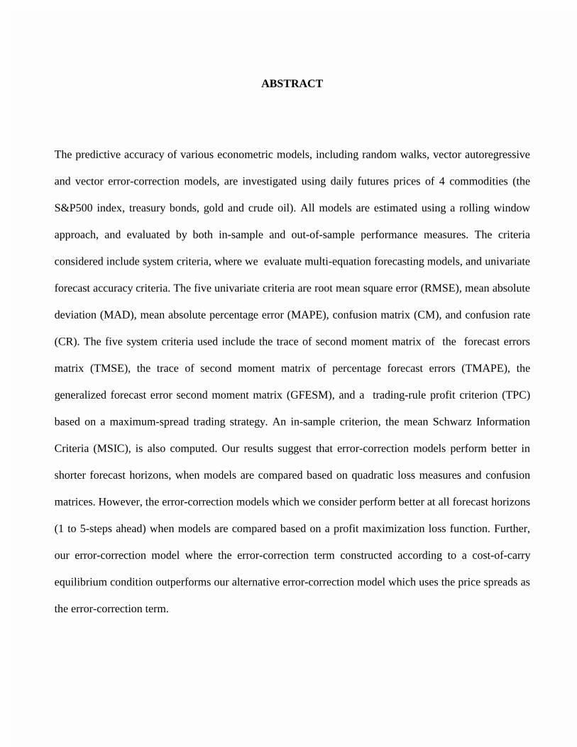
ABSTRACT
The predictive accuracy of various econometric models, including random walks, vector autoregressive
and vector error-correction models, are investigated using daily futures prices of 4 commodities (the
S&P500 index, treasury bonds, gold and crude oil). All models are estimated using a rolling window
approach, and evaluated by both in-sample and out-of-sample performance measures. The criteria
considered include system criteria, where we evaluate multi-equation forecasting models, and univariate
forecast accuracy criteria. The five univariate criteria are root mean square error (RMSE), mean absolute
deviation (MAD), mean absolute percentage error (MAPE), confusion matrix (CM), and confusion rate
(CR). The five system criteria used include the trace of second moment matrix of the forecast errors
matrix (TMSE), the trace of second moment matrix of percentage forecast errors (TMAPE), the
generalized forecast error second moment matrix (GFESM), and a trading-rule profit criterion (TPC)
based on a maximum-spread trading strategy. An in-sample criterion, the mean Schwarz Information
Criteria (MSIC), is also computed. Our results suggest that error-correction models perform better in
shorter forecast horizons, when models are compared based on quadratic loss measures and confusion
matrices. However, the error-correction models which we consider perform better at all forecast horizons
(1 to 5-steps ahead) when models are compared based on a profit maximization loss function. Further,
our error-correction model where the error-correction term constructed according to a cost-of-carry
equilibrium condition outperforms our alternative error-correction model which uses the price spreads as
the error-correction term.
2
1. Introduction
In recent years, there has been continued interest in the issue of the forecastability of future spot
prices using the term structure of futures prices. This research is motivated by both the need to test
economic theories, and by the desire to evaluate alternative forecasting strategies. In Fama and French
(1987) and French (1986), for example, the forecastability of futures prices are used as evidence to
support both the cost-of-carry equilibrium theory of Kaldor (1939), Working (1948), Brennan (1958) and
Telser (1958), where the basis (the difference between futures and spot prices) are explained by storage
costs and a convenience yield component, and the view that the basis can be explained by the expected
risk premium (Dusak (1973), Breeden (1980), and Hazuka (1984 ). In Bessembinder, Coughnour, Seguin
and Smoller (1995) and Swanson, Zeng and Kocagil (1996), forecastability of commodity prices is
related to mean reversions. Swanson and White (1995) evaluate the information in the term structure of
interest rates using linear and nonlinear models. Wahab, Cohn and Lashgari (1994) examine gold-silver
inter-markets arbitrage, based on predictions from cointegrating relationships. Lu and Leuthold (1994)
investigate cointegration relations among spot and futures prices of corn and soybeans, and related
implications for hedging and forecasting.
In this article, we examine the forecast performance of several models using daily futures prices for 4
commodities. The econometric models used include a random walk without drift (RW), a random walk
with drift (RWD), a vector autoregressive model with time trend (VAR), a vector error-correction
model with the price spread as the error-correction term (SPD), and a vector error-correction model with
the cost-of-carry as the error-correction term (COC). One question which we attempt to answer has been
previously addressed by Clements and Hendry (1995) and Hoffman and Rasche (1996), for example, is
3
what is the advantage of incorporating cointegrating relations in short and medium term forecasting
models. We also examine two different error-correction terms based on different theories.
To allow the term structure of prices to evolve over time, we estimate all models dynamically, using
fixed-length rolling windows of 250 days (approximately one year), and construct forecasts based on
forecast horizons of 1 day to 5 days (1-step ahead to 5-step ahead forecasts). The data used to forecast
prices is updated daily as new observation becomes available, and ex ante forecasts are constructed. The
results are then compared with true values, and out-of-sample forecasting errors are generated. Then, a
number of model selection criteria based on these errors are applied and analyzed. Such an approach,
often called a model selection approach, has advantages over the more traditional hypothesis testing
approach. One reason is that the approach allows us to focus on out-of-sample forecasting performance
without worrying about the specification of a correct model.
The model selection criteria considered in this paper include both full system criteria where multi-
equation forecast models are examined and univariate forecast evaluation criteria based on each variable
in the system. The five univariate criteria include root mean square error (RMSE), mean absolute
deviation (MAD), mean absolute percentage error (MAPE), confusion matrix (CM) and confusion rate
(CR). The five system criteria used include the trace of second moment matrix of forecast errors matrix
(TMSE), the trace of second moment matrix of percentage forecast errors (TMAPE), the generalized
forecast error second moment matrix (GFESM), as well as a trading-rule profit criterion (TPC) based on
a maximum-spread trading strategy. An in-sample criterion, the mean Schwarz information criterion
(MSIC), is also computed. Furthermore, we also conduct two statistical tests. One is based on the
confusion rate and tests whether a model is useful as a predictor of the sign of price changes. The other

4
test is the asymptotic loss differential test of Diebold and Mariano (1995), which examines whether two
models, are equally accurate based on predictive ability.
By adopting a model selection approach to commodity prices in a real time forecasting scenario, we
attempt to shed light on the usefulness of econometric forecasting, and the empirical relevance of
modeling theoretical relationships between futures and spot prices when constructing forecasting
models. Moreover, we propose a heuristic approach to modeling stochastic cointegration which is
implied by the cost-of-carry equilibrium, and find that these models outperform other models, which are
in many cases more parsimonious, especially when a profit measure is used to compare models. In
particular, our results suggest that error-correction models perform better in shorter forecast horizons,
when models are compared based on quadratic loss measures and confusion matrices. However, the
error-correction models which we consider perform better at all forecast horizons (1 to 5-steps ahead)
when models are compared based on a profit maximization loss function. Further, our error-correction
model where the error-correction term constructed according to a cost-of-carry equilibrium condition
outperforms our alternative error-correction model which uses price spreads as the error-correction
terms.
The rest of paper is organized as follows. Section 2 discusses data, while section 3 outlines the
forecasting models examined in this paper. Section 4 describes estimation strategies, and section 5
introduces the model selection criteria used. Section 6 summarizes the results and concludes.
2. Data

5
Daily settlement prices for four futures markets are employed. All price data are obtained from
Knight-Ridder Financial's CRB InfoTech Commodity database. Our samples include two mineral
contracts (crude oil, gold) and two financial contracts (treasury bonds and S&P500 index). Crude oil
data are from the New York Mercantile Exchange, gold data are from the New York Commodity
Exchange, treasury bonds data are from the Chicago Board of Trade, and the S&P500 index is from the
Chicago Mercantile Exchange.
Our sample period starts on 4/1/1990 and ends on 10/31/1995. The out-of-sample period used is
4/1/1991 to 10/31/1995. Thus, the first forecast (for 4/1/1991) is constructed based on in-sample
estimation using the period 4/1/1990 to 3/30/1991. The one-year in-sample size is chosen arbitrarily.
However, we don't expect that the results will be affected. In Swanson, Zeng and Kocagil (1996), we
used the same data with 3-month, 6-month and one-year in-sample sizes and did not find any effects
from choosing different in-sample sizes. Futures prices are collected for the active contract months of
the commodities, which are months 1-12 for crude oil, 2, 4, 6, 8, 10, 12 for gold, and 3, 6, 9, 12 for both
treasury bonds and the S&P500 index. Futures prices are ordered according to their maturity and are
called nearby prices, with nearby one corresponding to the nearest maturity, and nearby two referring to
contract with the second nearest maturity, etc. Several nearby price series are created for each
commodity. In particular, for crude oil, gold, and treasury bonds, eight nearby price series are created,
while three series for S&P500 index are created. Overall, the sample size is around 1400 for each
commodity.
According to Bessembinder et al. (1995), Bailey and Chan (1993), and Fama and French (1987), the
prices of first nearby futures contracts can be used to proxy for the spot price. Therefore, our analysis
6
based on the futures prices can also be extended to basis movements, or spreads between futures prices
and spot prices. One advantage of using futures prices is that we avoid problems which arise when
overlapping contracts are used, as well as problems associated with the volatility near the delivery
periods.
3. Forecasting Models
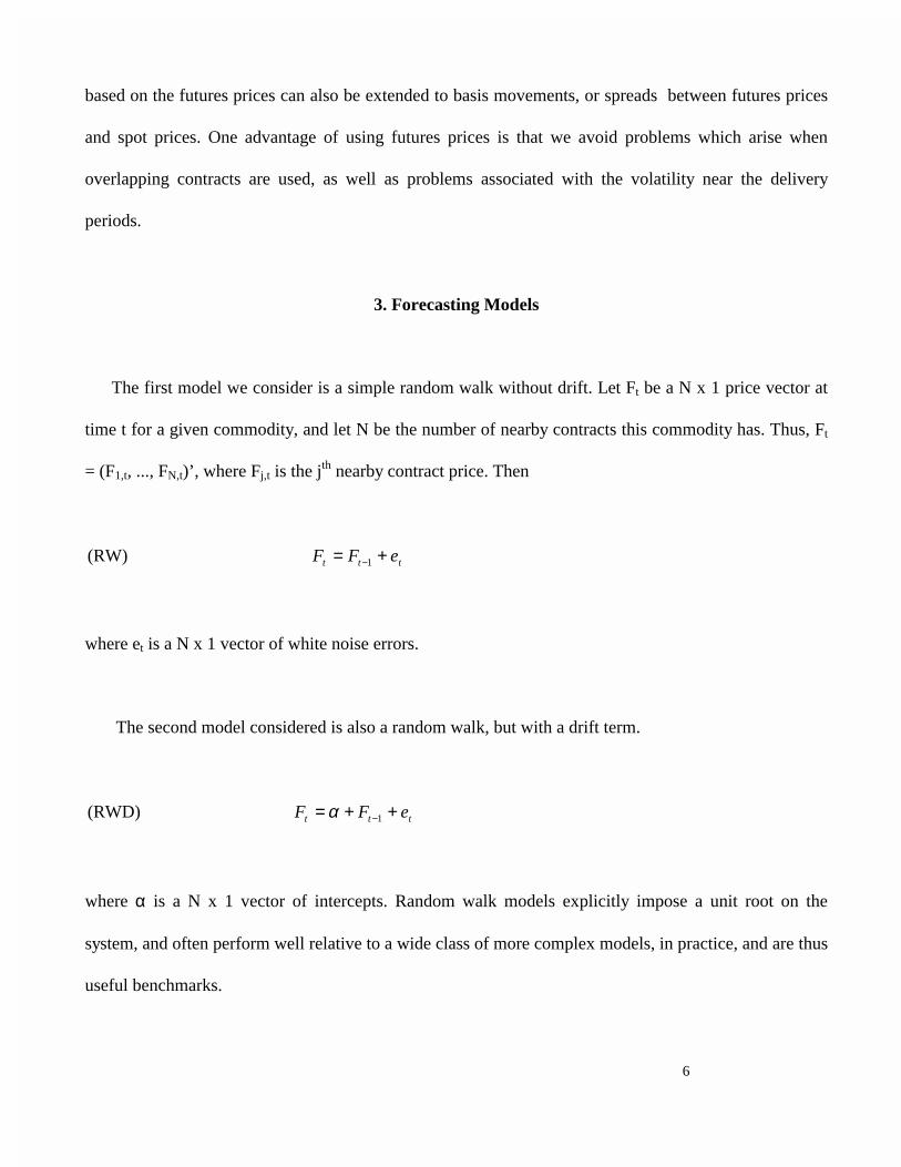
The first model we consider is a simple random walk without drift. Let Ft be a N x 1 price vector at
time t for a given commodity, and let N be the number of nearby contracts this commodity has. Thus, Ft
= (F1,t, ..., FN,t)’, where Fj,t is the jth nearby contract price. Then
(RW) 1 ttt eF F += −
where et is a N x 1 vector of white noise errors.
The second model considered is also a random walk, but with a drift term.
(RWD) 1 ttt eFF ++= −α
where α is a N x 1 vector of intercepts. Random walk models explicitly impose a unit root on the
system, and often perform well relative to a wide class of more complex models, in practice, and are thus
useful benchmarks.
7
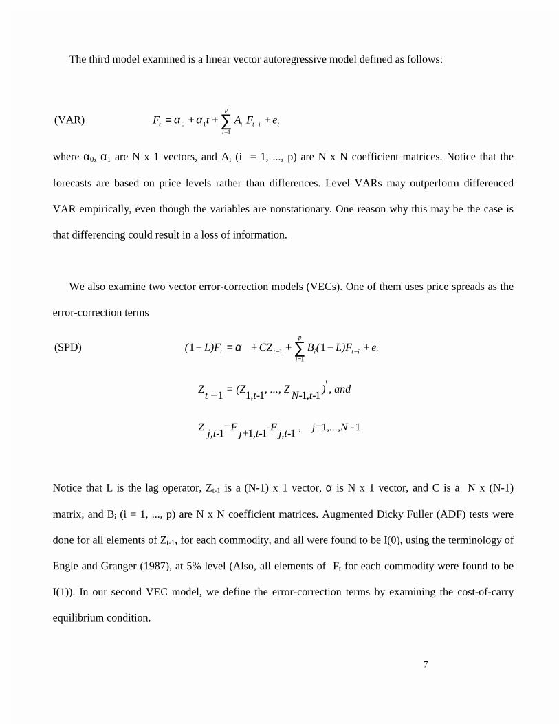
The third model examined is a linear vector autoregressive model defined as follows:
110 (VAR) tit
p
iit e FAtF +++= −
=∑αα
where α0, α1 are N x 1 vectors, and Ai (i = 1, ..., p) are N x N coefficient matrices. Notice that the
forecasts are based on price levels rather than differences. Level VARs may outperform differenced
VAR empirically, even though the variables are nonstationary. One reason why this may be the case is
that differencing could result in a loss of information.
We also examine two vector error-correction models (VECs). One of them uses price spreads as the
error-correction terms
11 11 (SPD) tit
p
iitt eL)F(BCZL)F( +−++=− −
=− ∑α
1.-11111
11111
,...,N , j=j,t-
-F,t-j+
=Fj,t-
Z
, and '),t-N-
, ..., Z,t-
= (Zt
Z −
Notice that L is the lag operator, Zt-1 is a (N-1) x 1 vector, α is N x 1 vector, and C is a N x (N-1)
matrix, and Bi (i = 1, ..., p) are N x N coefficient matrices. Augmented Dicky Fuller (ADF) tests were
done for all elements of Zt-1, for each commodity, and all were found to be I(0), using the terminology of
Engle and Granger (1987), at 5% level (Also, all elements of Ft for each commodity were found to be
I(1)). In our second VEC model, we define the error-correction terms by examining the cost-of-carry
equilibrium condition.
8
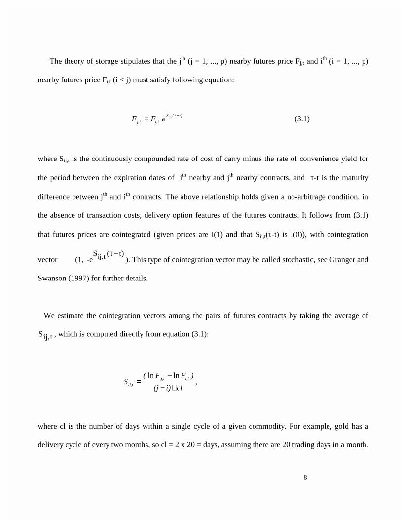
The theory of storage stipulates that the jth (j = 1, ..., p) nearby futures price Fj,t and ith (i = 1, ..., p)
nearby futures price Fi,t (i < j) must satisfy following equation:
(3.1) eF F t)(S
i,tj,tij,t −= τ
where Sij,t is the continuously compounded rate of cost of carry minus the rate of convenience yield for
the period between the expiration dates of ith nearby and jth nearby contracts, and τ-t is the maturity
difference between jth and ith contracts. The above relationship holds given a no-arbitrage condition, in
the absence of transaction costs, delivery option features of the futures contracts. It follows from (3.1)
that futures prices are cointegrated (given prices are I(1) and that Sij,t(τ-t) is I(0)), with cointegration
vector (1, -eS ( t)ij, t τ−
). This type of cointegration vector may be called stochastic, see Granger and
Swanson (1997) for further details.
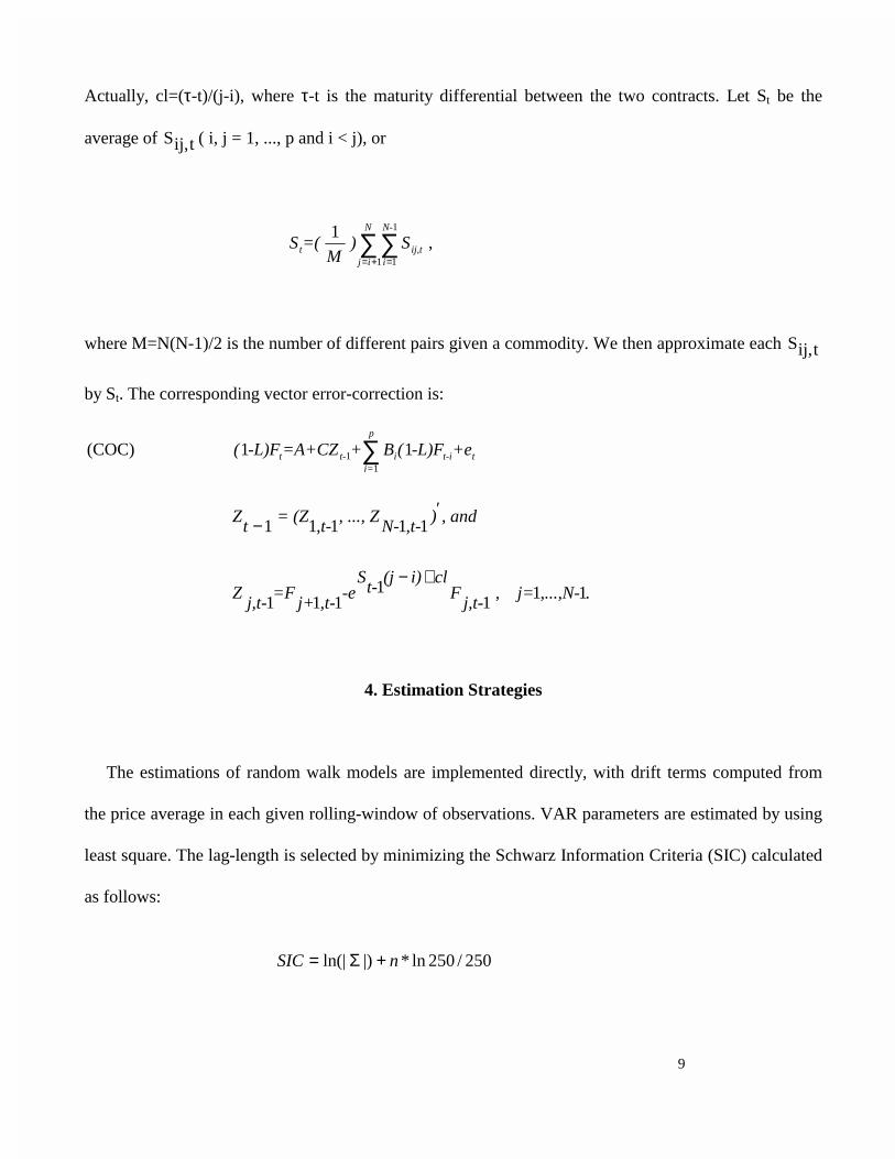
We estimate the cointegration vectors among the pairs of futures contracts by taking the average of
Sij,t , which is computed directly from equation (3.1):
cli)(j
)FF(S i,tj,t
ij,t ∗−−
=lnln
,
where cl is the number of days within a single cycle of a given commodity. For example, gold has a
delivery cycle of every two months, so cl = 2 x 20 = days, assuming there are 20 trading days in a month.
9
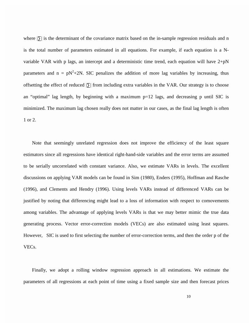
Actually, cl=(τ-t)/(j-i), where τ-t is the maturity differential between the two contracts. Let St be the
average of Sij,t ( i, j = 1, ..., p and i < j), or
∑∑+= =
N
ij
N-
iij,tt S)
M=(S
1
1
1
1,
where M=N(N-1)/2 is the number of different pairs given a commodity. We then approximate each Sij,t
by St. The corresponding vector error-correction is:
∑p
i=tt-iit-t +e-L)F(B+=A+CZ-L)F(
11 11 (COC)
. ,...,N- , j=j,t-
Fcli)(j
t-S
-e,t-j+
=Fj,t-
Z
, and '),t-N-
, ..., Z,t-
= (Zt
Z
111
1111
11111
∗−
−
4. Estimation Strategies
The estimations of random walk models are implemented directly, with drift terms computed from
the price average in each given rolling-window of observations. VAR parameters are estimated by using
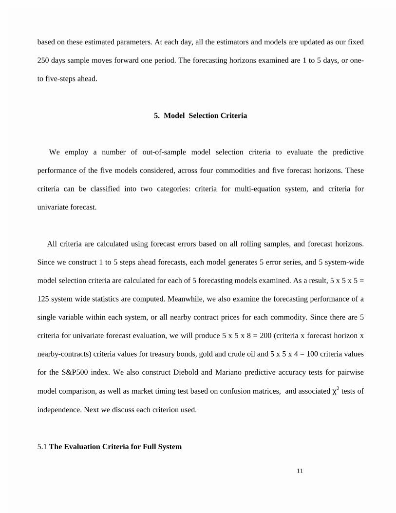
least square. The lag-length is selected by minimizing the Schwarz Information Criteria (SIC) calculated
as follows:
250/250ln*|)ln(| nSIC +Σ=
10
where |∑| is the determinant of the covariance matrix based on the in-sample regression residuals and n
is the total number of parameters estimated in all equations. For example, if each equation is a N-
variable VAR with p lags, an intercept and a deterministic time trend, each equation will have 2+pN
parameters and n = pN2+2N. SIC penalizes the addition of more lag variables by increasing, thus
offsetting the effect of reduced |∑| from including extra variables in the VAR. Our strategy is to choose
an “optimal” lag length, by beginning with a maximum p=12 lags, and decreasing p until SIC is
minimized. The maximum lag chosen really does not matter in our cases, as the final lag length is often
1 or 2.
Note that seemingly unrelated regression does not improve the efficiency of the least square
estimators since all regressions have identical right-hand-side variables and the error terms are assumed
to be serially uncorrelated with constant variance. Also, we estimate VARs in levels. The excellent
discussions on applying VAR models can be found in Sim (1980), Enders (1995), Hoffman and Rasche
(1996), and Clements and Hendry (1996). Using levels VARs instead of differenced VARs can be
justified by noting that differencing might lead to a loss of information with respect to comovements
among variables. The advantage of applying levels VARs is that we may better mimic the true data
generating process. Vector error-correction models (VECs) are also estimated using least squares.
However, SIC is used to first selecting the number of error-correction terms, and then the order p of the
VECs.
Finally, we adopt a rolling window regression approach in all estimations. We estimate the
parameters of all regressions at each point of time using a fixed sample size and then forecast prices
11
based on these estimated parameters. At each day, all the estimators and models are updated as our fixed
250 days sample moves forward one period. The forecasting horizons examined are 1 to 5 days, or one-
to five-steps ahead.
5. Model Selection Criteria
We employ a number of out-of-sample model selection criteria to evaluate the predictive
performance of the five models considered, across four commodities and five forecast horizons. These
criteria can be classified into two categories: criteria for multi-equation system, and criteria for
univariate forecast.
All criteria are calculated using forecast errors based on all rolling samples, and forecast horizons.
Since we construct 1 to 5 steps ahead forecasts, each model generates 5 error series, and 5 system-wide
model selection criteria are calculated for each of 5 forecasting models examined. As a result, 5 x 5 x 5 =
125 system wide statistics are computed. Meanwhile, we also examine the forecasting performance of a
single variable within each system, or all nearby contract prices for each commodity. Since there are 5
criteria for univariate forecast evaluation, we will produce 5 x 5 x 8 = 200 (criteria x forecast horizon x
nearby-contracts) criteria values for treasury bonds, gold and crude oil and 5 x 5 x 4 = 100 criteria values
for the S&P500 index. We also construct Diebold and Mariano predictive accuracy tests for pairwise
model comparison, as well as market timing test based on confusion matrices, and associated χ2 tests of
independence. Next we discuss each criterion used.
5.1 The Evaluation Criteria for Full System
12
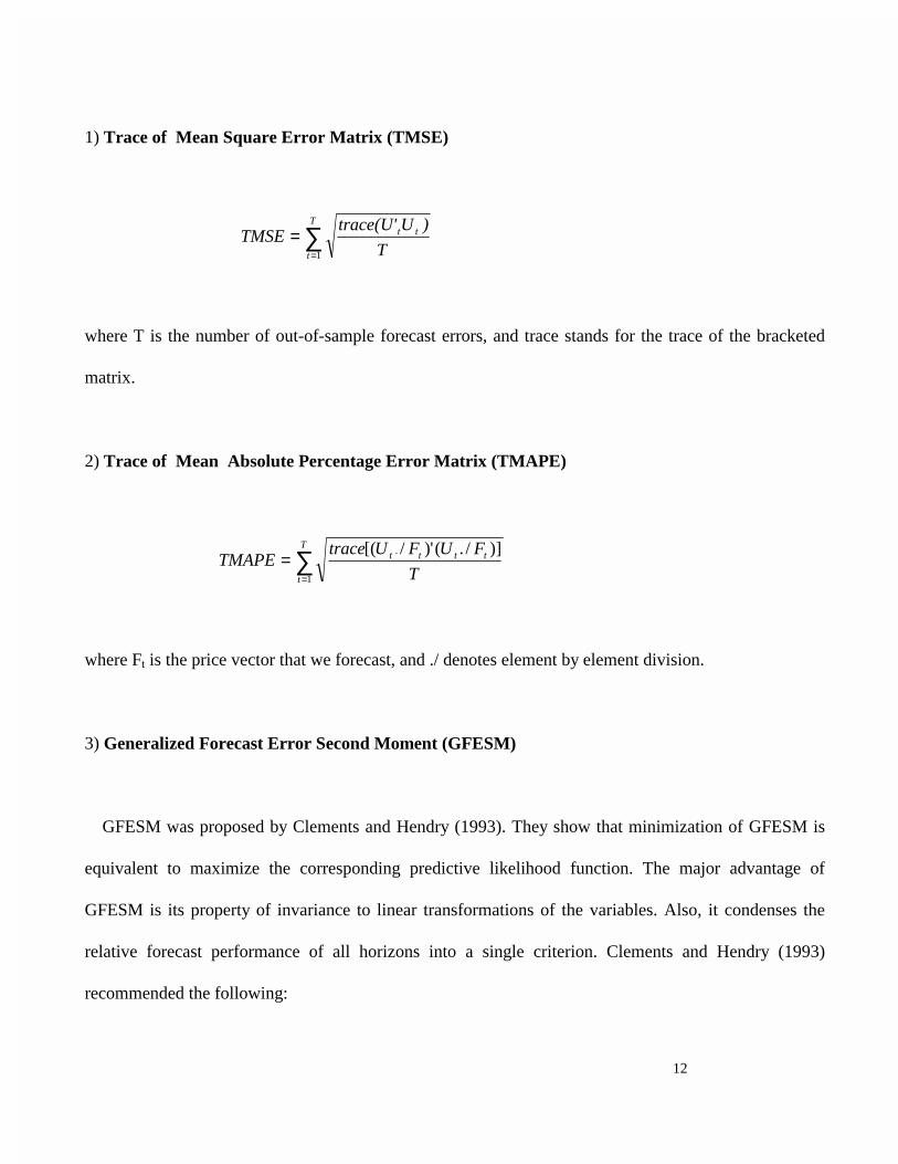
1) Trace of Mean Square Error Matrix (TMSE)
∑=
=T
t
tt
T
)Utrace(U'TMSE
1
where T is the number of out-of-sample forecast errors, and trace stands for the trace of the bracketed
matrix.
2) Trace of Mean Absolute Percentage Error Matrix (TMAPE)
∑=
=T
t
tttt
T
FUFUtraceTMAPE
1
. )]/.()'/[(
where Ft is the price vector that we forecast, and ./ denotes element by element division.
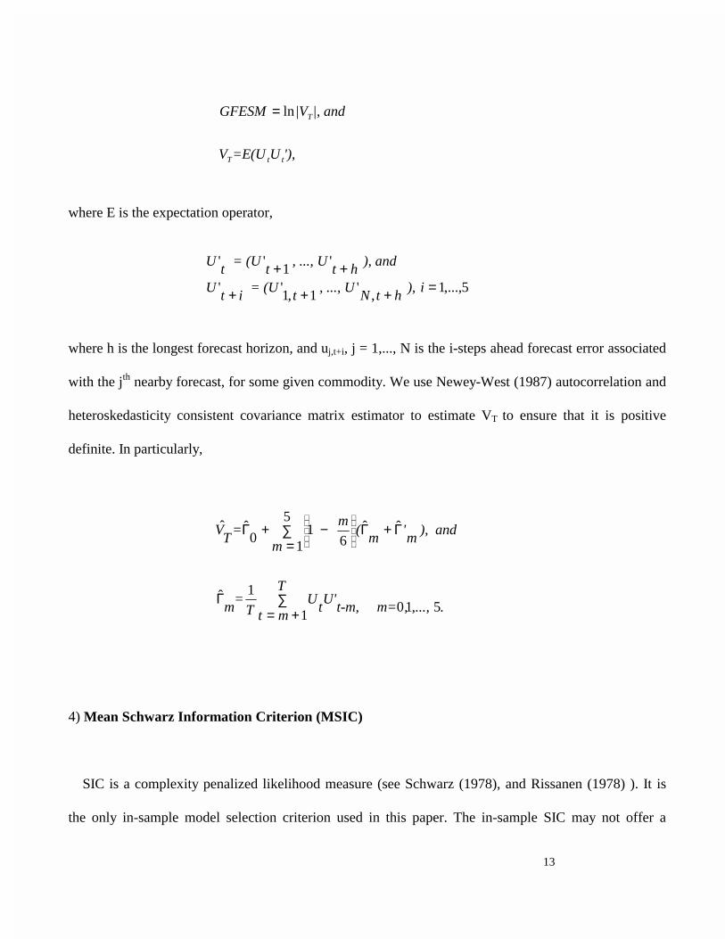
3) Generalized Forecast Error Second Moment (GFESM)
GFESM was proposed by Clements and Hendry (1993). They show that minimization of GFESM is
equivalent to maximize the corresponding predictive likelihood function. The major advantage of
GFESM is its property of invariance to linear transformations of the variables. Also, it condenses the
relative forecast performance of all horizons into a single criterion. Clements and Hendry (1993)
recommended the following:
13
'),U=E(UV
|, and|VGFESM
ttT
Tln=
where E is the expectation operator,
where h is the longest forecast horizon, and uj,t+i, j = 1,..., N is the i-steps ahead forecast error associated
with the jth nearby forecast, for some given commodity. We use Newey-West (1987) autocorrelation and
heteroskedasticity consistent covariance matrix estimator to estimate VT to ensure that it is positive
definite. In particularly,
. ,..., ,=t-m, mU'
T
mtt
UT
=m
), andm
'm
(m
m =
TV
5101
1ˆ
ˆˆ 5
1 61
0ˆˆ
∑+=
Γ
Γ+Γ∑=
−+Γ
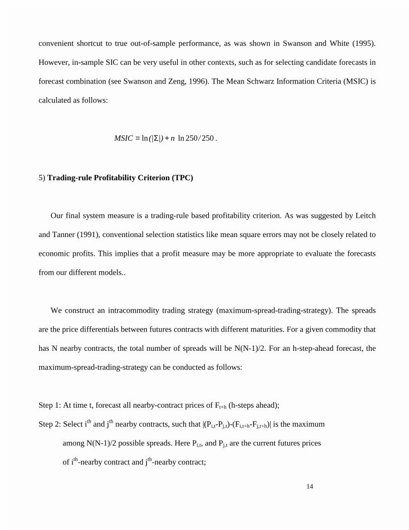
4) Mean Schwarz Information Criterion (MSIC)
SIC is a complexity penalized likelihood measure (see Schwarz (1978), and Rissanen (1978) ). It is
the only in-sample model selection criterion used in this paper. The in-sample SIC may not offer a
5,...,1 ,
'1,1
''
'1
''
=+++
++i),
htN, ..., U
t = (U
itU
), and ht
, ..., Ut
= (Ut
U
14
convenient shortcut to true out-of-sample performance, as was shown in Swanson and White (1995).
However, in-sample SIC can be very useful in other contexts, such as for selecting candidate forecasts in
forecast combination (see Swanson and Zeng, 1996). The Mean Schwarz Information Criteria (MSIC) is
calculated as follows:
250250lnln /n |)(|MSIC +Σ= .
5) Trading-rule Profitability Criterion (TPC)
Our final system measure is a trading-rule based profitability criterion. As was suggested by Leitch
and Tanner (1991), conventional selection statistics like mean square errors may not be closely related to
economic profits. This implies that a profit measure may be more appropriate to evaluate the forecasts
from our different models..
We construct an intracommodity trading strategy (maximum-spread-trading-strategy). The spreads
are the price differentials between futures contracts with different maturities. For a given commodity that
has N nearby contracts, the total number of spreads will be N(N-1)/2. For an h-step-ahead forecast, the
maximum-spread-trading-strategy can be conducted as follows:
Step 1: At time t, forecast all nearby-contract prices of Ft+h (h-steps ahead);
Step 2: Select ith and jth nearby contracts, such that |(Pi,t-Pj,t)-(Fi,t+h-Fj,t+h)| is the maximum
among N(N-1)/2 possible spreads. Here Pi,t, and Pj,t are the current futures prices
of ith-nearby contract and jth-nearby contract;

15
Step 3: At time t, short spread of (Pi,t-Pj,t), when (Pi,t-Pj,t)-(Fi,t+h-Fj,t+h) is positive; or short
spread of (Pj,t-Pi,t), when (Pi,t-Pj,t)-(Fi,t+h-Fj,t+h) is negative;
Step 4: At t+h, long the same spread and cash-in the “profit”;
Step 5: Repeat the step 1 to 4 and accumulate the losses or profits until the sample expires.
Thus, one examines comparable spreads of contracts maturing at different dates for the same
commodity. If one spread is anticipated to fluctuate most, then, either long or short that spread today
depending upon the direction of forecasts, and take the opposite position in the same spread next period.
Note that the above rule is a buy-and-hold strategy, where the arbitrageurs during each day enter into
offsetting positions against the spread taken h-days ago. This may not be the best strategy though, since
the position taken based on forecasts h days ago will not be updated as extra data becomes available.
One reason we didn’t use a more sophisticated strategy is that we are more interested in the forecasting
accuracy of the different models for the given forecast horizon. The transaction costs are not considered.
However, we expect that evaluation of the relative performance of different models should not be
affected by this omission, since our strategy restricts trading volume to one unit per day, and more
importantly all models involve the same trading frequency. Also, the capital requirement for mark-to-
market should not be a problem as the holding periods are short and the offsetting position will always
be taken cyclically. Overall, though, capital availability is not a trivial question in a spread-based trading
strategy. A more detailed discussion can be found in Abken (1989). Other questions affecting the
implementation of a trading strategy involve the potential illiquidity issues, and problems associated
with the delivery periods of futures contracts. These are ignored in this study. An overview of the similar
issues can be found in Ma, Mercer, and Walker (1992).
16
Finally, one possible reason why a spread-based trading strategy could result in a positive profit is
mean reversion. A partial list of relevant literature where this issue is discussed includes Cecchetti, Lam
and Mark (1990), Fama and French (1988), Kim, Nelson and Startz (1991), Miller, Muthwamy and
Whaley (1994), as well as Bessembinder, Coughenour, Seguin and Smoller (1995) and Swanson, Zeng
and Kocagil (1996).
5.2 Evaluation Criteria for Univariate Forecasts
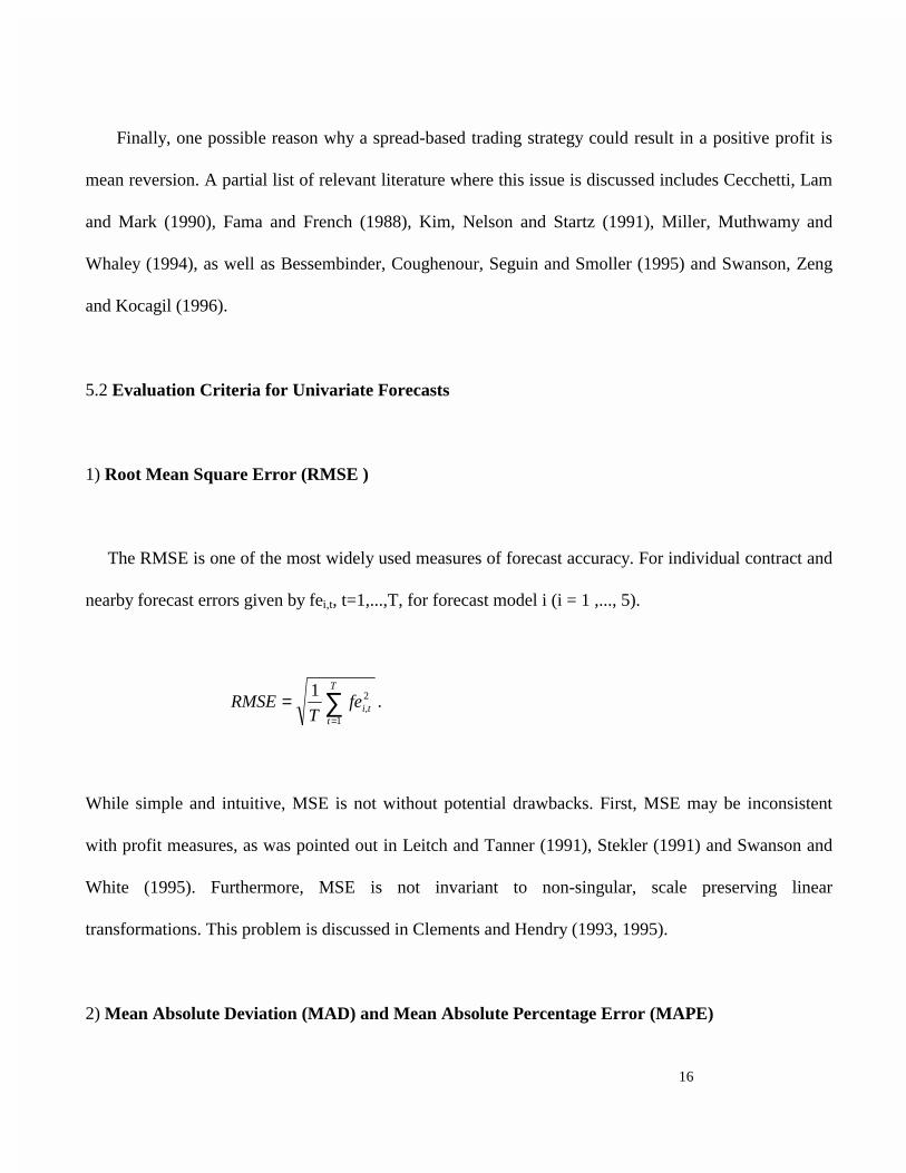
1) Root Mean Square Error (RMSE )
The RMSE is one of the most widely used measures of forecast accuracy. For individual contract and
nearby forecast errors given by fei,t, t=1,...,T, for forecast model i (i = 1 ,..., 5).
∑=
=T
ti,tfe
TRMSE
1
21.
While simple and intuitive, MSE is not without potential drawbacks. First, MSE may be inconsistent
with profit measures, as was pointed out in Leitch and Tanner (1991), Stekler (1991) and Swanson and
White (1995). Furthermore, MSE is not invariant to non-singular, scale preserving linear
transformations. This problem is discussed in Clements and Hendry (1993, 1995).
2) Mean Absolute Deviation (MAD) and Mean Absolute Percentage Error (MAPE)
17
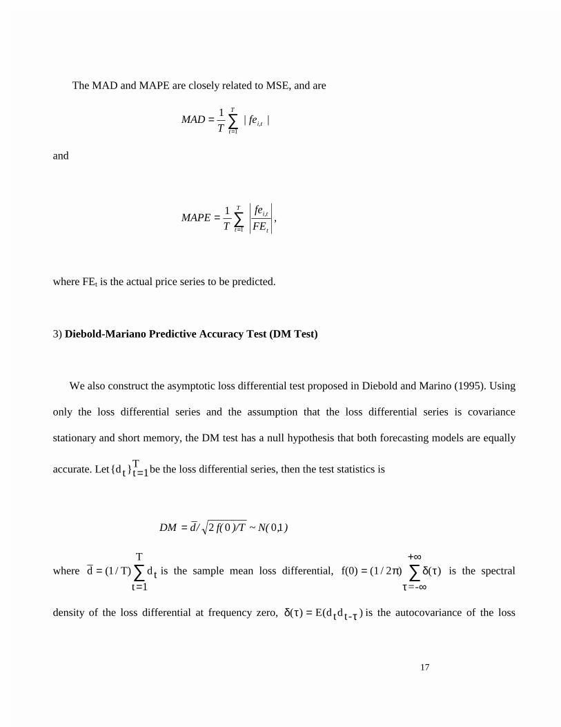
The MAD and MAPE are closely related to MSE, and are
∑=
=T
ti,t | | fe
TMAD
1
1
and
t
i,tT
t FE
fe
TMAPE ∑
=
=1
1,
where FEt is the actual price series to be predicted.
3) Diebold-Mariano Predictive Accuracy Test (DM Test)
We also construct the asymptotic loss differential test proposed in Diebold and Marino (1995). Using
only the loss differential series and the assumption that the loss differential series is covariance
stationary and short memory, the DM test has a null hypothesis that both forecasting models are equally
accurate. Let{d t}t 1T= be the loss differential series, then the test statistics is
), ~ N()/Tf(/dDM 1002=
where d T d tt
T=
=∑( / )1
1
is the sample mean loss differential, f(0) (1 / 2 ) ( )
=-
=∞
+∞∑π δ τ
τis the spectral
density of the loss differential at frequency zero, δ τ τ( ) E d td t-= ( ) is the autocovariance of the loss
18
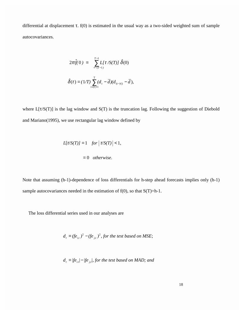
differential at displacement τ. f(0) is estimated in the usual way as a two-sided weighted sum of sample
autocovariances.
∑−
−−=
=1
1
(0)ˆ0ˆ2T
)(T
/S(T)] L[) (f δτπ
∑+=
− −−=T
1||t|)|(t ),1)(ˆ
τττδ d)(dd(d/T)( t
where L[τ/S(T)] is the lag window and S(T) is the truncation lag. Following the suggestion of Diebold
and Mariano(1995), we use rectangular lag window defined by
se. otherwi
S(T) for S(T)]L
0
1, / 1/[
=
<= ττ
Note that assuming (h-1)-dependence of loss differentials for h-step ahead forecasts implies only (h-1)
sample autocovariances needed in the estimation of f(0), so that S(T)=h-1.
The loss differential series used in our analyses are
;22 on MSEtest based, for the )(fe)(fed j,ti,tt −=
andd on MAD; test base|, for the|fe||fed j,ti.tt −=
19
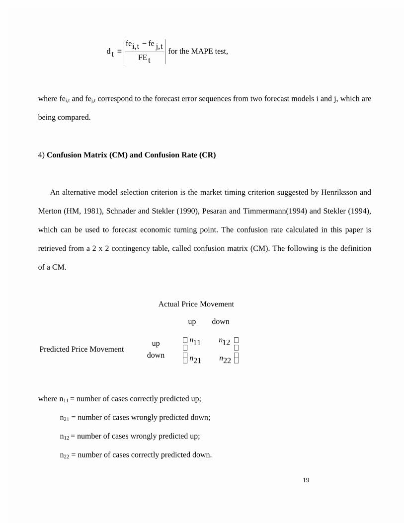
d tfei,t fe j,t
FEt for the MAPE test,=
−
where fei,t and fej,t correspond to the forecast error sequences from two forecast models i and j, which are
being compared.
4) Confusion Matrix (CM) and Confusion Rate (CR)
An alternative model selection criterion is the market timing criterion suggested by Henriksson and
Merton (HM, 1981), Schnader and Stekler (1990), Pesaran and Timmermann(1994) and Stekler (1994),
which can be used to forecast economic turning point. The confusion rate calculated in this paper is
retrieved from a 2 x 2 contingency table, called confusion matrix (CM). The following is the definition
of a CM.
Actual Price Movement
up down
Predicted Price Movement up
down
n n
n n
11 12
21 22
where n11 = number of cases correctly predicted up;
n21 = number of cases wrongly predicted down;
n12 = number of cases wrongly predicted up;
n22 = number of cases correctly predicted down.
20
The confusion rate is then computed as the frequency of off-diagonal elements, or
)/Tn(nCR 2112 += ,
where T = n11+ n12+ n21+ n22. The best model according to CR is the least confused one---the one with
the smallest value of CR.
Pesaran and Timmermann (1994) showed that the test of market timing (in the context of forecasting
the direction of asset price movements) proposed by HM is asymptotically equivalent to the standard χ2
test of independence in a confusion matrix, when the column and row sums are not a priori fixed, which
is the case in this analysis. We examine the standard χ2 test of independence. The null hypothesis is
independence between the actual and the predicted directions. Thus, rejecting the null hypothesis
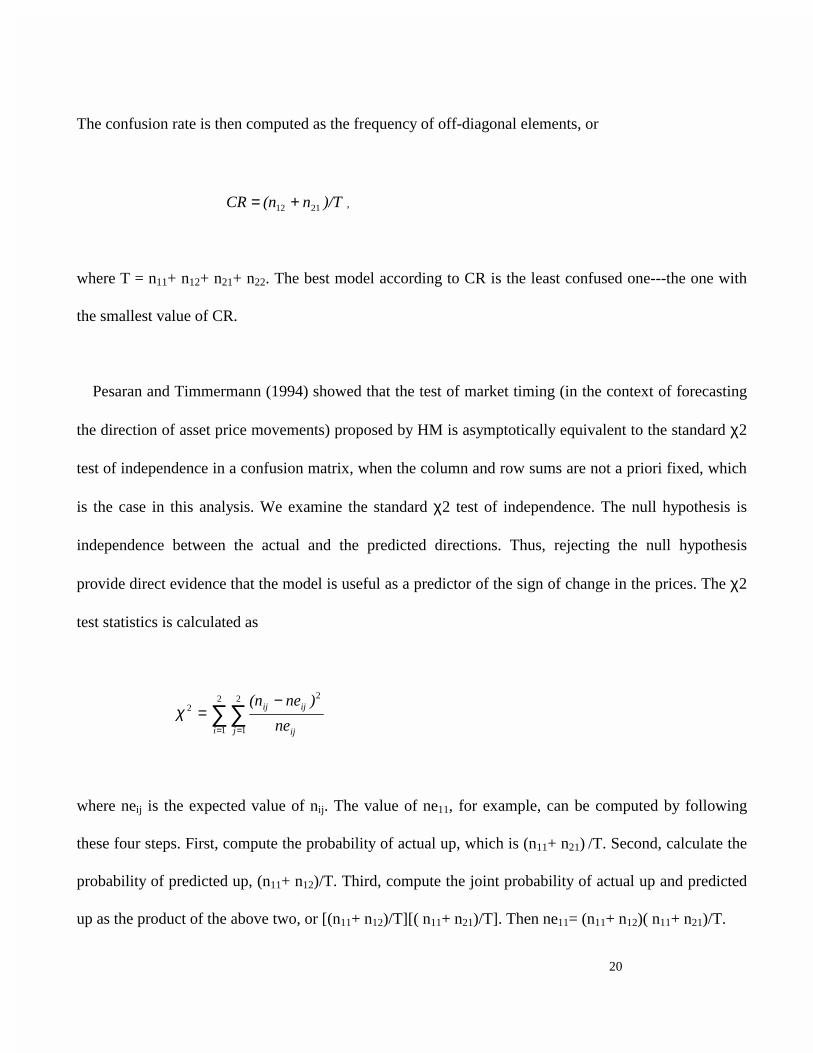
provide direct evidence that the model is useful as a predictor of the sign of change in the prices. The χ2
test statistics is calculated as
∑∑= =
−=
2
1
2
1
22
i j ij
ijij
ne
)ne(nχ
where neij is the expected value of nij. The value of ne11, for example, can be computed by following
these four steps. First, compute the probability of actual up, which is (n11+ n21) /T. Second, calculate the
probability of predicted up, (n11+ n12)/T. Third, compute the joint probability of actual up and predicted
up as the product of the above two, or [(n11+ n12)/T][( n11+ n21)/T]. Then ne11= (n11+ n12)( n11+ n21)/T.

21
Similarly, ne22= (n12+ n22)(n21+ n22)/T,
ne12= (n11+ n12)( n12+ n22)/T and
ne21=(n11+ n12)(n21+ n22)/T.
6. Forecast Performance
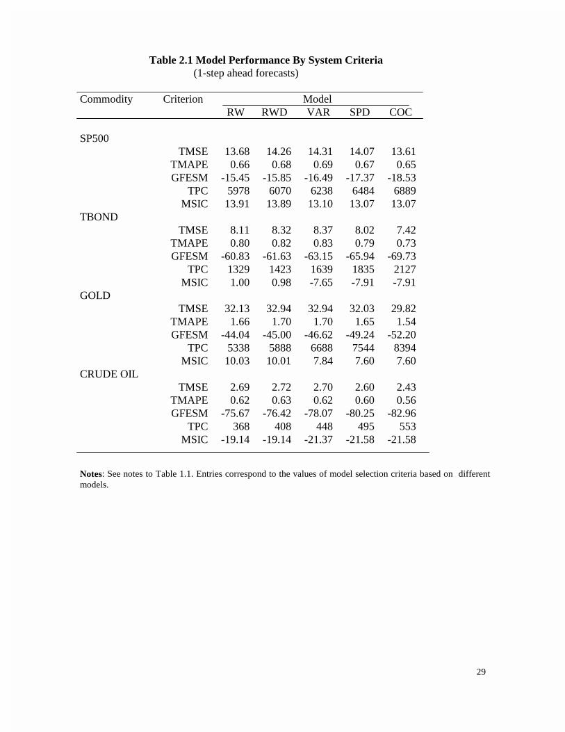
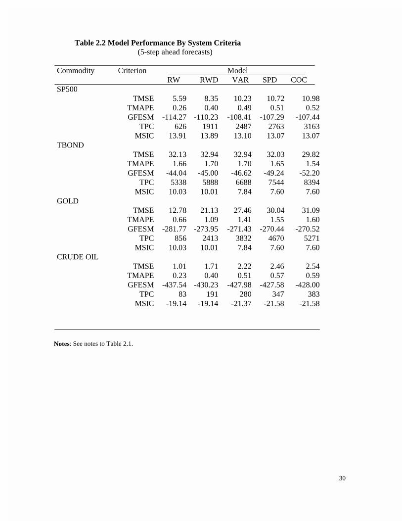
This section discusses empirical results reported in Tables 1 to 5. Tables 1 and 2 present the results
from system-based criteria. In particular, Table 1 reports the rankings of each model and Table 2 reports
the criteria values upon which these rankings are based. Tables 3 and 4 give our forecasting results for
univariate forecasts based model selection criteria. In particular, Table 3 reports the relative rankings and
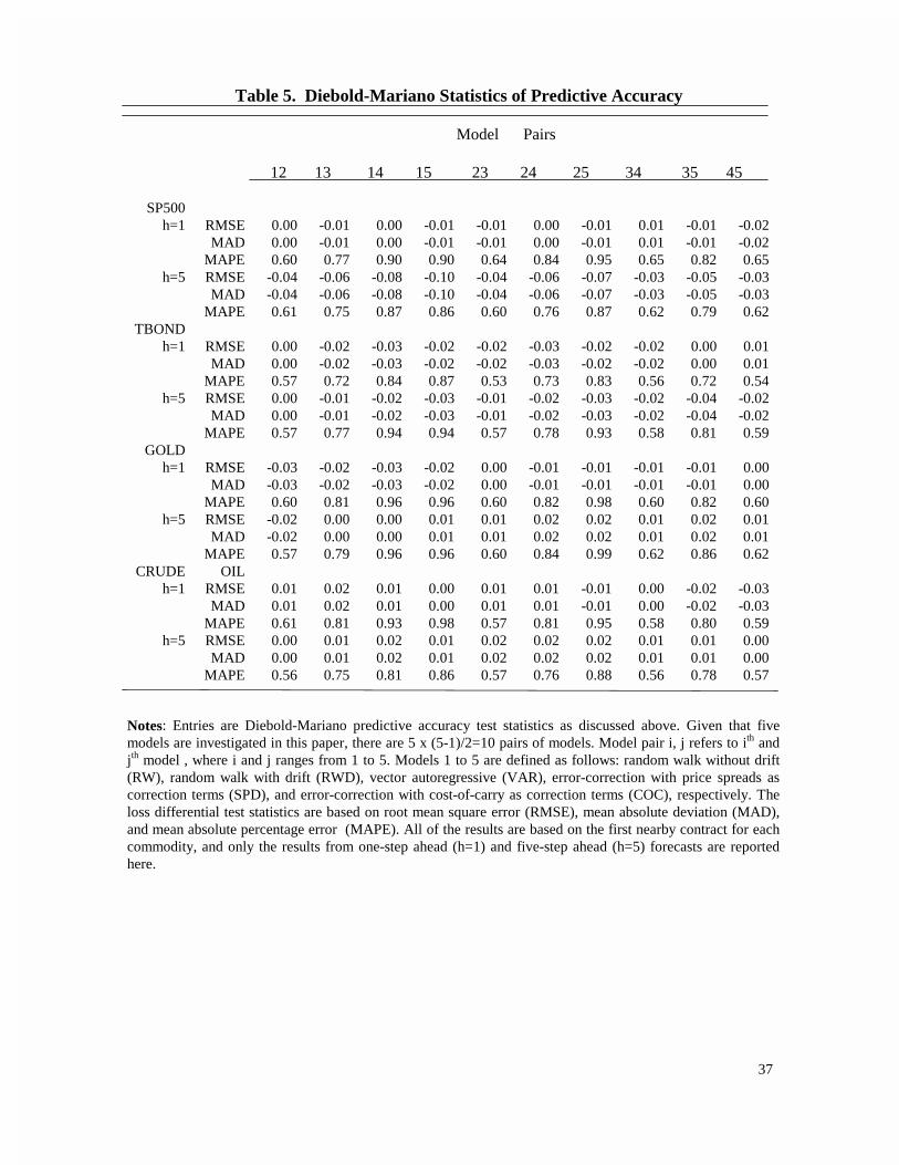
Table 4 contains the criteria values. Finally, Table 5 reports the pairwise model comparison statistics
based on Diebold-Mariano predictive accuracy tests for all the commodities and their nearbies. Only the
results from one step ahead and five step ahead forecasts are reported here, but the results for two to
four step ahead forecasts are available upon request.
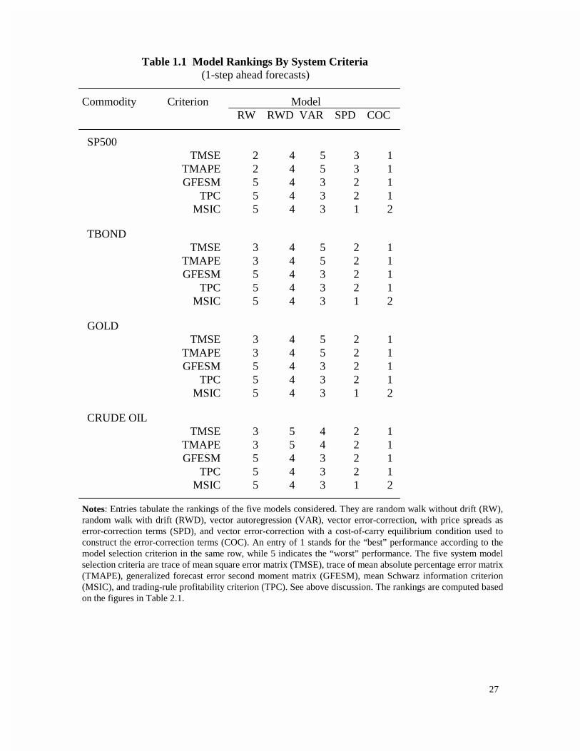
The entries in Table 1.1 and 1.2 represent the rankings of our five models based on the five different
system model selection criteria, and four different commodities. A ranking of number 1 stands for the
best model with respect to the corresponding model selection criterion, while 5 stands for the worst
model, etc.Table 1.1 suggests, first, that error-correction models dominate based on all criteria for one-
step ahead forecasts. Between the two error-correction models, COC outperforms SPD except based on
the in-sample MSIC. Second, random walk models outperform VAR based on the criteria of TMSE,
TMAPE, but underperform VAR based on GFESM and TPC in one-step-ahead forecasts. Also, adding

22
drift terms to the random walk models does not improve the forecasting performance based on TMSE
and TMAPE, although the reverse is true based on all other model selection criteria. Third, from Table
2.1, note that the profits, based on TPC, differ by up to 60% for one-step-ahead forecasts across models.
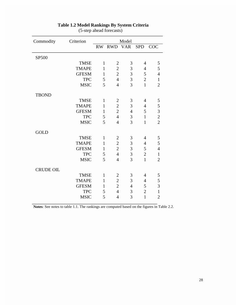
As the forecast horizon is increased, the error-correction models lose their dominance (see Table
1.5), and random walk models perform best when based on criteria other than TPC and MSIC. However,
for our profit measure (TPC), the error-correction models continue to outperform all others. This is
indicative of the importance of specifying appropriate loss functions, based on the needs of each
individual end-users of our forecasts.
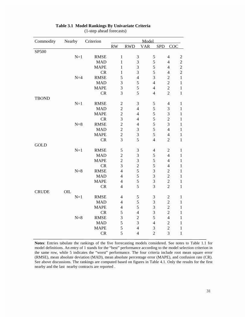
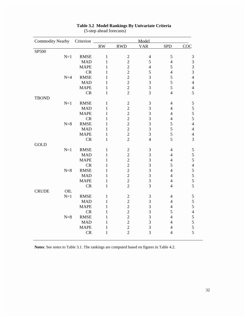
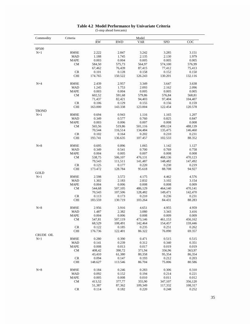
Tables 3.1 and 3.2 report the rankings of all models and the values univariate model selection criteria
based on one-step amd five-step ahead forecasts. Table 5 reports the results from DM test statistics. In
all of these tables, only the results from the most recent nearby and most distant nearby futures contracts
are reported, for the sake of brevity.
The conclusions based on the examination of in table 3.1 are quite similar to the results discussed
above for system criteria, as error-correction models still dominate all others for one-step ahead
forecasts. Overall, though, the rankings among different criteria are more consistent than those based on
system-wide criteria. In particular, relative rankings for first nearby and distant nearby are the same.
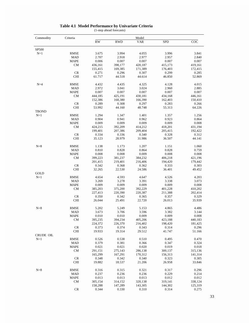
Table 4 reports the values of all univariate criteria, for all commodities and forecast horizons.
Judging by the CR values, it is interesting to note that all models are actually quite accurate, correctly
predict the direction of price changes around 70% of time. While S&P500 has the lowest CR values,
23
treasury bonds has the largest. At 10% significance level, all of the χ2 values suggest rejecting the null
hypothesis of statistical independence. In other words, all models are useful for predicting the direction
of price changes. Entries in Table 5 are the Diebold-Mariano statistics. At 10% significance level, all
DM statistics suggest accepting the null hypothesis (i.e. each pairs of models are equally accurate in
terms of prediction).
7. Summary and Conclusion
In this paper, we investigate the predictive accuracy of five econometric models. All models are
estimated using a rolling window approach, so that our evaluations are based on the dynamic out-of-
sample forecast performance. The criteria considered include both system and univariate model selection
criteria. For a given commodity, our system includes all traded nearby futures contracts.
Our results suggest that error-correction models perform better in shorter forecast horizons, when
models are compared based on quadratic loss measures and confusion matrices. However, the error-
correction models which we consider perform better at all forecast horizons (1 to 5-steps ahead) when
models are compared based on a profit maximization loss function. Further, our error-correction model
where the error-correction term constructed according to a cost-of-carry equilibrium condition
outperforms our alternative error-correction model which uses the price spreads as the error-correction
term.
24
References
Abken, P. A.(1989): "An Analysis of Intra-Market Spreads in Heating Oil Futures," Journal Of Futures Market, Vol. 9, #1, April, 1989.
Akaike, H.(1973): "Information Theory and an Extension of the Maximum Likelihood Principle," in B. N. Petrov and F. Csaki, eds., 2nd International Symposium on Information Theory (Budapest: Akademiai Kiado), 267-281.
Akaike, H.(1974): "A New Look at the Statistical Model Identification," IEEE Transactions on Automatic Control AC-19, 716-23.
Bailey, W. and K. C. Chan(1993): "Macroeconomic Influences and the Variability of the Commodity Futures Basis," Journal of Finance 48, 555-573.
Bessembinder, H., Coughenour, J.F., Seguin, P.J. and M.M. Smoller(1995): "Mean Reversion in Equilibrium Asset Prices: Evidence from the Futures Term Structure," Journal of Finance 50, 361-375.
Brennan, M.J.(1958): "The Theory of Storage: American Economic Review," 48, 50-72.
Cecchetti, S., Lam, P. and N., Mark(1990): "Mean Reversion in Equilibrium Asset Prices," The American Economic Review 80, 399-418.
Clements, M.P. and D.F. Hendry(1993): "On the Limitations of Comparing Mean Square Forecast Errors," Journal of Forecasting, 12, 617-676.
Clements, M.P. and D.F. Hendry(1995): "Forecasting in cointegrated system," Journal of Applied Econometrics, 10, 127-146.
Dusak, K. C.(1990): "Futures Trading and Investor Returns: An Investigation of Commodity Market Risk Premiums," Journal of Political Economy 81, 1387-1406.
Diebold, Francis X. and Roberto S. Marino(1995): " Comparing Predictive Accuracy," Journal of Business and Economic Statistics 13, 253-263.
Enders, Walter.(1995): Applied Econometric Time Series, John Wiley & Sons, Inc.
Engle, R.F. and S.J. Brown(1986): "Model Selection for Forecasting," Applied Mathematics and Computation 20.
Engle, R.F. and C.W.J. Granger(1987): "Co-integration And Error Correction: Representation, Estimation, and Testing," Econometrica 55, 251-76.
Fama, E.F. and K.R. French(1987): "Commodity Futures Prices: Some Evidence on Forecast Power, Premiums, and the Theory of Storage,"
25
Journal of Business 60, 55-73.
Fama, E.F. and K.R. French(1988): "Business Cycles and the Behavior of Metals Prices," Journal of Finance 43, 1075-1093.
French, K.R.(1986): "Detecting Spot Price Forecasts in Futures Prices," Journal of Business 59, 39-54.
Granger, C. WJ. and N. Swanson(1997): "Stochastic cointegration," Oxford Bulletin of Economics and Statistics, 59:2, 23-35.
Hazuka, T. B.(1984): "Consumption Betas and Normal Backwarwardation in Commodity Markets", Journal of Finance 39, 647-655.
Henriksson, R.D. and Merton, R.C.(1981): "On Market Timing and Investment Performance II: Statistical Procedures for Evaluating Forecast Skills," Journal of Business, 54, 513-533.
Hoffman, D and R. Rasche(1996): "Assessing forecast performance in a cointegration system," Journal of Applied Econometrics. Vol. 11, 495-517.
Kaldor, N.(1939): "Speculation and Economic Stability," Review of Economic Studies 7, 1-27.
Kim, M.J., Nelson, C.R. and R. Startz(1991): "Mean Reversion in Stock Prices? A Reappraisal of the Empirical Evidence," Review of Economic Studies 58, 515-528.
Leitch , G. and Tanner, J.E.(1991): "Economic Forecast Evaluation: Profits Versus the Conventional Error Measures," American Economic Review, 81, 580-590.
Lin, J. and R.S. Tsay(1996): "Co-integration Constraint and Forecasting : An Empirical Examination," Journal of Applied Econometric, Vol. 11, 519-538.
Lu, R. and R. M. Leuthold(1994): "Cointegration Relations between Spot and Futures Prices for Storable Commodities: Implications for Hedging and Forecasting," OFOR working paper 94-12, University of Illinois at Urbana-Champaign.
Ma, C, Mercer, J. and M.A. Walker(1992): "Rolling Over Futures Contracts: A Note," Journal of Futures Market, Vol. 12, #12, April.
Miller, M.H., Muthuswamy, J. and R.E. Whaley(1994): "Mean Reversion of Standard & Poor's 500 Index Based Changes: Arbitrage-induced or Statistical Illusion," Journal of Finance 49, 479-513.
Newey, W. K., and K. D. West(1987): "A Simple Positive Semi-Definite, Heteroskedasticity and Autocorrelation Consistent Covariance Matrix," Econometrica, 55: 703-8.
26
Pesaran, M.H. and A.G. Timmermann(1994): "A Generalization of the non-parametric Henriksson-Merton Test of Market Timing," Economics Letters, 44, 1-7.
Rissanen, Jorma(1978): "Modeling by Shortest Data Description," Automatica 14, 465-471.
Schnader, M.H. and Stekler, H. O.(1990): "Evaluating Predictions of Change," Journal of Business, 63, 99-107.
Schwarz, Gideon(1978): "Estimating the Dimension of a Model," The Annals of Statistics 6, 461-464.
Sim, Christopher(1980): "Macroeconomics and Reality," Econometrica, 48, Jan., 1-49.
Stekler, H. O.(1991): "Macroeconomic Forecast Evaluation Techniques," International Journal of Forecasting, 7, 375-384.
Stekler, H. O.(1994): "Are Economic Forecasts Valuable?" Journal of Forecasting, Vol. 13, 495-505.
Swanson, N.R. and H. White(1995): "A Model Selection Approach to Assessing the Information in the Term Structure Using Linear Models and Artificial Neural Networks," Journal of Business and Economic Statistics 13, 265-275.
Swanson, N.R. and H. White(1997): "A Model Selection Approach to Real-Time Macroeconomic Forecasting Using Linear Models and Artificial Neural Networks," Review of Economics and Statistics, Vol. 79, issue 4.
Swanson, N.R. and T. Zeng(1996): "Addressing Colineararity Among Competing Econometric Forecasts: Regression Based Forecast Combination Using Model Selection," Working Paper, Penn State University.
Swanson, N.R., T. Zeng and A. E. Kocagil(1996): "The Probability of Mean Reversion in Equilibrium Asset Prices and Returns," Working Paper, Penn State University.
Telser, L.G.(1958): "Futures Trading and the Storage of Cotton and Wheat," Journal of Political Economy 66, 233-255.
Wahab, M., R. Cohn and M. Lashgari(1994): "Gold-Silver Spread: Integration,Cointegration, Predictability, ex ante Arbitrage," Journal of Futures Market, Vol. 14, #6.
West, K.D.(1995): "Asymptotic Inference About Predictive Ability," forthcoming, Econometrica.
Working, H.(1949): "The Theory of the Price of Storage," American Economic Review 39, 1254-1262.
27
Table 1.1 Model Rankings By System Criteria (1-step ahead forecasts)
Commodity Criterion Model RW RWD VAR SPD COC
SP500TMSE 2 4 5 3 1
TMAPE 2 4 5 3 1GFESM 5 4 3 2 1
TPC 5 4 3 2 1MSIC 5 4 3 1 2
TBONDTMSE 3 4 5 2 1
TMAPE 3 4 5 2 1GFESM 5 4 3 2 1
TPC 5 4 3 2 1MSIC 5 4 3 1 2
GOLDTMSE 3 4 5 2 1
TMAPE 3 4 5 2 1GFESM 5 4 3 2 1
TPC 5 4 3 2 1MSIC 5 4 3 1 2
CRUDE OILTMSE 3 5 4 2 1
TMAPE 3 5 4 2 1GFESM 5 4 3 2 1
TPC 5 4 3 2 1MSIC 5 4 3 1 2
Notes: Entries tabulate the rankings of the five models considered. They are random walk without drift (RW),random walk with drift (RWD), vector autoregression (VAR), vector error-correction, with price spreads aserror-correction terms (SPD), and vector error-correction with a cost-of-carry equilibrium condition used toconstruct the error-correction terms (COC). An entry of 1 stands for the “best” performance according to themodel selection criterion in the same row, while 5 indicates the “worst” performance. The five system modelselection criteria are trace of mean square error matrix (TMSE), trace of mean absolute percentage error matrix(TMAPE), generalized forecast error second moment matrix (GFESM), mean Schwarz information criterion(MSIC), and trading-rule profitability criterion (TPC). See above discussion. The rankings are computed basedon the figures in Table 2.1.
28
Table 1.2 Model Rankings By System Criteria (5-step ahead forecasts)
Commodity Criterion Model RW RWD VAR SPD COC
SP500TMSE 1 2 3 4 5
TMAPE 1 2 3 4 5GFESM 1 2 3 5 4
TPC 5 4 3 2 1MSIC 5 4 3 1 2
TBONDTMSE 1 2 3 4 5
TMAPE 1 2 3 4 5GFESM 1 2 4 5 3
TPC 5 4 3 1 2MSIC 5 4 3 1 2
GOLDTMSE 1 2 3 4 5
TMAPE 1 2 3 4 5GFESM 1 2 3 5 4
TPC 5 4 3 2 1MSIC 5 4 3 1 2
CRUDE OILTMSE 1 2 3 4 5
TMAPE 1 2 3 4 5GFESM 1 2 4 5 3
TPC 5 4 3 2 1MSIC 5 4 3 1 2
Notes: See notes to table 1.1. The rankings are computed based on the figures in Table 2.2.
29
Table 2.1 Model Performance By System Criteria (1-step ahead forecasts)
Commodity Criterion Model RW RWD VAR SPD COC
SP500TMSE 13.68 14.26 14.31 14.07 13.61
TMAPE 0.66 0.68 0.69 0.67 0.65GFESM -15.45 -15.85 -16.49 -17.37 -18.53
TPC 5978 6070 6238 6484 6889MSIC 13.91 13.89 13.10 13.07 13.07
TBONDTMSE 8.11 8.32 8.37 8.02 7.42
TMAPE 0.80 0.82 0.83 0.79 0.73GFESM -60.83 -61.63 -63.15 -65.94 -69.73
TPC 1329 1423 1639 1835 2127MSIC 1.00 0.98 -7.65 -7.91 -7.91
GOLDTMSE 32.13 32.94 32.94 32.03 29.82
TMAPE 1.66 1.70 1.70 1.65 1.54GFESM -44.04 -45.00 -46.62 -49.24 -52.20
TPC 5338 5888 6688 7544 8394MSIC 10.03 10.01 7.84 7.60 7.60
CRUDE OILTMSE 2.69 2.72 2.70 2.60 2.43
TMAPE 0.62 0.63 0.62 0.60 0.56GFESM -75.67 -76.42 -78.07 -80.25 -82.96
TPC 368 408 448 495 553MSIC -19.14 -19.14 -21.37 -21.58 -21.58
Notes: See notes to Table 1.1. Entries correspond to the values of model selection criteria based on differentmodels.
30
Table 2.2 Model Performance By System Criteria (5-step ahead forecasts)
Commodity Criterion Model RW RWD VAR SPD COCSP500
TMSE 5.59 8.35 10.23 10.72 10.98TMAPE 0.26 0.40 0.49 0.51 0.52GFESM -114.27 -110.23 -108.41 -107.29 -107.44
TPC 626 1911 2487 2763 3163MSIC 13.91 13.89 13.10 13.07 13.07
TBONDTMSE 32.13 32.94 32.94 32.03 29.82
TMAPE 1.66 1.70 1.70 1.65 1.54GFESM -44.04 -45.00 -46.62 -49.24 -52.20
TPC 5338 5888 6688 7544 8394MSIC 10.03 10.01 7.84 7.60 7.60
GOLDTMSE 12.78 21.13 27.46 30.04 31.09
TMAPE 0.66 1.09 1.41 1.55 1.60GFESM -281.77 -273.95 -271.43 -270.44 -270.52
TPC 856 2413 3832 4670 5271MSIC 10.03 10.01 7.84 7.60 7.60
CRUDE OILTMSE 1.01 1.71 2.22 2.46 2.54
TMAPE 0.23 0.40 0.51 0.57 0.59GFESM -437.54 -430.23 -427.98 -427.58 -428.00
TPC 83 191 280 347 383MSIC -19.14 -19.14 -21.37 -21.58 -21.58
Notes: See notes to Table 2.1.
31
Table 3.1 Model Rankings By Univariate Criteria (1-step ahead forecasts)
Commodity Nearby Criterion Model RW RWD VAR SPD COCSP500
N=1 RMSE 1 3 5 4 2MAD 1 3 5 4 2
MAPE 1 3 5 4 2CR 1 3 5 4 2
N=4 RMSE 5 4 3 2 1MAD 3 5 4 2 1
MAPE 3 5 4 2 1CR 3 5 4 2 1
TBONDN=1 RMSE 2 3 5 4 1
MAD 2 4 5 3 1MAPE 2 4 5 3 1
CR 3 4 5 2 1N=8 RMSE 2 4 5 3 1
MAD 2 3 5 4 1MAPE 2 3 5 4 1
CR 3 5 4 2 1GOLD
N=1 RMSE 5 3 4 2 1MAD 2 3 5 4 1
MAPE 2 3 5 4 1CR 3 2 5 4 1
N=8 RMSE 4 5 3 2 1MAD 4 5 3 2 1
MAPE 4 5 3 2 1CR 4 5 3 2 1
CRUDE OILN=1 RMSE 4 5 3 2 1
MAD 4 5 3 2 1MAPE 4 5 3 2 1
CR 5 4 3 2 1N=8 RMSE 3 2 5 4 1
MAD 5 3 4 2 1MAPE 5 4 3 2 1
CR 5 4 2 3 1
Notes: Entries tabulate the rankings of the five forrecasting models considered. See notes to Table 1.1 formodel definitions. An entry of 1 stands for the “best” performance according to the model selection criterion inthe same row, while 5 indicates the “worst” performance. The four criteria include root mean square error(RMSE), mean absolute deviation (MAD), mean absolute percentage error (MAPE), and confusion rate (CR).See above discussions. The rankings are computed based on figures in Table 4.1. Only the results for the firstnearby and the last nearby contracts are reported .
32
Table 3.2 Model Rankings By Univariate Criteria (5-step ahead forecasts)
Commodity Nearby Criterion Model RW RWD VAR SPD COCSP500
N=1 RMSE 1 2 4 5 3MAD 1 2 5 4 3
MAPE 1 2 4 5 3CR 1 2 5 4 3
N=4 RMSE 1 2 3 5 4MAD 1 2 3 5 4
MAPE 1 2 3 5 4CR 1 2 3 4 5
TBONDN=1 RMSE 1 2 3 4 5
MAD 1 2 3 4 5MAPE 1 2 3 4 5
CR 1 2 3 4 5N=8 RMSE 1 2 3 5 4
MAD 1 2 3 5 4MAPE 1 2 3 5 4
CR 1 2 4 5 3GOLD
N=1 RMSE 1 2 3 4 5 MAD 1 2 3 4 5MAPE 1 2 3 4 5
CR 1 2 3 5 4N=8 RMSE 1 2 3 4 5
MAD 1 2 3 4 5MAPE 1 2 3 4 5
CR 1 2 3 4 5CRUDE OIL
N=1 RMSE 1 2 3 4 5 MAD 1 2 3 4 5MAPE 1 2 3 4 5
CR 1 2 3 5 4N=8 RMSE 1 2 3 4 5
MAD 1 2 3 4 5MAPE 1 2 3 4 5
CR 1 2 3 4 5
Notes: See notes to Table 3.1. The rankings are computed based on figures in Table 4.2.
33
Table 4.1 Model Performance by Univariate Criteria (1-step ahead forecasts)
Commodity Criteria Model RW RWD VAR SPD COC
SP500 N=1 RMSE 3.675 3.994 4.055 3.996 3.841
MAD 2.707 2.918 2.977 2.957 2.840MAPE 0.006 0.007 0.007 0.007 0.007
CM 436,161 398,177 420,187 415,173 419,161 155,415 169,385 171,389 176,403 172,415
CR 0.271 0.296 0.307 0.299 0.285 CHI 61.717 44.518 44.614 46.850 52.869
N=4 RMSE 4.432 4.435 4.325 4.128 4.015 MAD 2.972 3.041 3.024 2.960 2.885MAPE 0.007 0.007 0.007 0.007 0.007
CM 444,185 425,191 430,181 434,168 446,161 152,386 168,380 166,390 162,403 150,410
CR 0.289 0.308 0.297 0.283 0.266 CHI 53.992 44.160 48.748 55.313 64.226
TBOND N=1 RMSE 1.294 1.347 1.401 1.357 1.256
MAD 0.904 0.941 0.962 0.923 0.864MAPE 0.009 0.009 0.009 0.009 0.008
CM 424,215 392,209 414,212 418,201 431,194 199,401 207,386 209,404 205,415 192,422
CR 0.334 0.336 0.340 0.328 0.312 CHI 35.123 28.979 31.986 36.507 44.141
N=8 RMSE 1.138 1.173 1.207 1.151 1.060 MAD 0.810 0.828 0.864 0.828 0.759MAPE 0.008 0.008 0.009 0.008 0.008
CM 399,223 381,237 384,232 406,218 421,196 201,415 219,401 216,406 194,420 179,442
CR 0.342 0.368 0.362 0.333 0.303 CHI 32.265 22.530 24.586 36.401 49.452
GOLD N=1 RMSE 4.654 4.593 4.647 4.526 4.203
MAD 3.269 3.278 3.391 3.338 3.073MAPE 0.009 0.009 0.009 0.009 0.008
CM 385,203 375,200 392,229 401,228 410,202 227,413 220,390 220,387 211,388 202,414
CR 0.350 0.342 0.365 0.357 0.329 CHI 26.044 25.491 22.720 26.013 35.939
N=8 RMSE 5.202 5.249 5.153 4.865 4.486 MAD 3.673 3.706 3.596 3.382 3.144MAPE 0.010 0.010 0.009 0.009 0.008
CM 395,235 394,234 405,206 423,188 440,183 224,372 226,370 216,402 198,420 181,425
CR 0.373 0.374 0.343 0.314 0.296 CHI 19.933 19.314 29.512 41.747 51.166
CRUDE OIL N=1 RMSE 0.526 0.538 0.510 0.495 0.470
MAD 0.379 0.381 0.366 0.347 0.324MAPE 0.021 0.021 0.020 0.019 0.018
CM 291,151 275,143 286,138 300,137 315,136 165,299 167,291 170,312 156,313 141,314
CR 0.348 0.342 0.340 0.323 0.305 CHI 19.882 18.537 21.206 26.958 33.846
N=8 RMSE 0.316 0.315 0.321 0.317 0.296 MAD 0.237 0.236 0.236 0.229 0.214MAPE 0.013 0.013 0.013 0.012 0.012
CM 305,154 314,152 320,138 319,141 338,124 158,288 147,289 143,305 144,302 125,319
CR 0.344 0.330 0.310 0.314 0.275

34
CHI 21.547 25.946 32.256 30.888 45.770Notes: Entries correspond to the values of univariate model selection criteria. See notes to Table 3.1. Only the results based on the firstnearby (N=1) and the last nearby (N=4, for SP500, and N=8 for others) are reported here.
35
Table 4.2 Model Performance by Univariate Criteria (5-step ahead forecasts)
Commodity Criteria Model RW RWD VAR SPD COC
SP500 N=1 RMSE 2.222 2.847 3.242 3.285 3.151
MAD 1.188 1.745 2.135 2.130 1.979 MAPE 0.003 0.004 0.005 0.005 0.005
CM 584,50 575,73 564,97 574,100 576,99 67,462 76,439 87,415 77,412 75,413
CR 0.101 0.128 0.158 0.152 0.150 CHI 174.765 150.522 126.243 130.201 132.116
N=4 RMSE 2.439 2.957 3.349 3.647 3.638 MAD 1.245 1.753 2.093 2.162 2.096 MAPE 0.003 0.004 0.005 0.005 0.005
CM 602,52 591,68 579,86 576,84 568,81 71,437 82,421 94,403 97,404 104,407
CR 0.106 0.129 0.155 0.156 0.159 CHI 163.000 143.338 123.004 122.454 120.578
TBOND N=1 RMSE 0.694 0.943 1.116 1.165 1.207
MAD 0.349 0.577 0.760 0.825 0.847 MAPE 0.003 0.006 0.007 0.008 0.008
CM 565,56 519,86 501,116 499,124 488,139 70,544 116,514 134,484 135,475 146,460
CR 0.102 0.164 0.202 0.210 0.231 CHI 193.741 136.635 107.457 102.533 88.352
N=8 RMSE 0.695 0.896 1.065 1.142 1.127 MAD 0.349 0.541 0.700 0.769 0.758 MAPE 0.004 0.005 0.007 0.008 0.008
CM 538,75 506,107 476,131 468,136 470,123 79,543 111,511 141,487 148,482 147,492
CR 0.125 0.177 0.220 0.230 0.219 CHI 173.472 128.784 95.618 88.708 94.927
GOLD N=1 RMSE 2.598 3.572 4.175 4.462 4.576
MAD 1.302 2.183 2.832 3.102 3.154 MAPE 0.004 0.006 0.008 0.008 0.009
CM 544,68 507,105 486,129 464,140 470,141 70,543 107,506 128,482 149,471 142,470
CR 0.113 0.173 0.210 0.236 0.231 CHI 183.559 130.719 103.264 84.431 88.283
N=8 RMSE 2.956 3.916 4.651 4.955 4.959 MAD 1.487 2.382 3.080 3.343 3.416 MAPE 0.004 0.006 0.008 0.009 0.009
CM 547,81 507,119 473,146 461,153 456,162 68,529 108,491 142,464 154,457 159,446
CR 0.122 0.185 0.235 0.251 0.262 CHI 176.736 122.401 86.322 76.090 69.357
CRUDE OIL N=1 RMSE 0.280 0.390 0.471 0.515 0.515
MAD 0.141 0.239 0.312 0.340 0.351 MAPE 0.008 0.013 0.017 0.019 0.019
CM 408,42 390,72 371,94 356,96 363,97 43,410 61,380 80,358 95,354 86,354
CR 0.094 0.147 0.193 0.212 0.203 CHI 148.627 113.546 86.704 75.006 80.586
N=8 RMSE 0.184 0.246 0.283 0.306 0.310 MAD 0.092 0.152 0.194 0.214 0.221 MAPE 0.005 0.008 0.010 0.011 0.012
CM 413,52 377,77 355,90 347,107 356,120 51,387 87,362 109,349 117,332 108,317
CR 0.114 0.182 0.220 0.248 0.252

36
CHI 134.103 90.366 68.790 56.323 55.538
Notes: See notes to Table 4.1.
37
Table 5. Diebold-Mariano Statistics of Predictive Accuracy
Model Pairs
12 13 14 15 23 24 25 34 35 45
SP500 h=1 RMSE 0.00 -0.01 0.00 -0.01 -0.01 0.00 -0.01 0.01 -0.01 -0.02
MAD 0.00 -0.01 0.00 -0.01 -0.01 0.00 -0.01 0.01 -0.01 -0.02MAPE 0.60 0.77 0.90 0.90 0.64 0.84 0.95 0.65 0.82 0.65
h=5 RMSE -0.04 -0.06 -0.08 -0.10 -0.04 -0.06 -0.07 -0.03 -0.05 -0.03 MAD -0.04 -0.06 -0.08 -0.10 -0.04 -0.06 -0.07 -0.03 -0.05 -0.03MAPE 0.61 0.75 0.87 0.86 0.60 0.76 0.87 0.62 0.79 0.62
TBOND h=1 RMSE 0.00 -0.02 -0.03 -0.02 -0.02 -0.03 -0.02 -0.02 0.00 0.01
MAD 0.00 -0.02 -0.03 -0.02 -0.02 -0.03 -0.02 -0.02 0.00 0.01MAPE 0.57 0.72 0.84 0.87 0.53 0.73 0.83 0.56 0.72 0.54
h=5 RMSE 0.00 -0.01 -0.02 -0.03 -0.01 -0.02 -0.03 -0.02 -0.04 -0.02 MAD 0.00 -0.01 -0.02 -0.03 -0.01 -0.02 -0.03 -0.02 -0.04 -0.02MAPE 0.57 0.77 0.94 0.94 0.57 0.78 0.93 0.58 0.81 0.59
GOLD h=1 RMSE -0.03 -0.02 -0.03 -0.02 0.00 -0.01 -0.01 -0.01 -0.01 0.00
MAD -0.03 -0.02 -0.03 -0.02 0.00 -0.01 -0.01 -0.01 -0.01 0.00MAPE 0.60 0.81 0.96 0.96 0.60 0.82 0.98 0.60 0.82 0.60
h=5 RMSE -0.02 0.00 0.00 0.01 0.01 0.02 0.02 0.01 0.02 0.01 MAD -0.02 0.00 0.00 0.01 0.01 0.02 0.02 0.01 0.02 0.01MAPE 0.57 0.79 0.96 0.96 0.60 0.84 0.99 0.62 0.86 0.62
CRUDE OIL h=1 RMSE 0.01 0.02 0.01 0.00 0.01 0.01 -0.01 0.00 -0.02 -0.03
MAD 0.01 0.02 0.01 0.00 0.01 0.01 -0.01 0.00 -0.02 -0.03MAPE 0.61 0.81 0.93 0.98 0.57 0.81 0.95 0.58 0.80 0.59
h=5 RMSE 0.00 0.01 0.02 0.01 0.02 0.02 0.02 0.01 0.01 0.00 MAD 0.00 0.01 0.02 0.01 0.02 0.02 0.02 0.01 0.01 0.00MAPE 0.56 0.75 0.81 0.86 0.57 0.76 0.88 0.56 0.78 0.57
Notes: Entries are Diebold-Mariano predictive accuracy test statistics as discussed above. Given that fivemodels are investigated in this paper, there are 5 x (5-1)/2=10 pairs of models. Model pair i, j refers to ith andjth model , where i and j ranges from 1 to 5. Models 1 to 5 are defined as follows: random walk without drift(RW), random walk with drift (RWD), vector autoregressive (VAR), error-correction with price spreads ascorrection terms (SPD), and error-correction with cost-of-carry as correction terms (COC), respectively. Theloss differential test statistics are based on root mean square error (RMSE), mean absolute deviation (MAD),and mean absolute percentage error (MAPE). All of the results are based on the first nearby contract for eachcommodity, and only the results from one-step ahead (h=1) and five-step ahead (h=5) forecasts are reportedhere.