Recent Developments in Econometric Modeling and …epubs.surrey.ac.uk/7525/2/recent developments.pdfRecent Developments in Econometric Modeling and Forecasting GANG LI a, HAIYAN SONG

1

Recent Developments in Econometric Modeling and

Forecasting

GANG LI a, HAIYAN SONG

b and STEPHEN F. WITT

a *

a School of Management, University of Surrey, Guildford GU2 7XH, United Kingdom b School of Hotel and Tourism Management, The Hong Kong Polytechnic University,

Hung Hom, Kowloon, Hong Kong

Eighty-four post-1990 empirical studies of international tourism demand modeling

and forecasting using econometric approaches are reviewed. New developments

are identified and it is shown that applications of advanced econometric methods

improve the understanding of international tourism demand. An examination of the

22 studies which compare forecasting performance suggests that no single

forecasting method can outperform the alternatives in all cases. However, the time-

varying parameter (TVP) model and structural time series model with causal

variables perform consistently well.

Keywords: review, tourism demand, modeling, forecasting

INTRODUCTION

The rapid expansion of international tourism has motivated growing interest in

tourism demand studies. The earliest work of can be traced back to the 1960s, notably

pioneered by Guthrie (1961), followed by Gerakis (1965) and Gray (1966). The last

four decades have seen great developments in tourism demand analysis, in terms of

the diversity of research interests, the depth of theoretical foundations, and advances

in research methodologies. Modeling tourism demand in order to analyze the effects

of various determinants, and accurate forecasting of future tourism demand, are two

major focuses of tourism demand studies. The developments in tourism forecasting

methodologies fall into several streams, amongst which the econometric approach

plays a very important role in tourism demand studies. This methodology is able to

interpret the causes of variations of tourism demand, support policy evaluation and

strategy making, and predict future trends in tourism development.

Since the beginning of the 1960s a large number of empirical studies on tourism

demand have been published. Crouch (1994c) carried out an extensive literature

search and found over 300 publications during the period 1961-1993. Since then about

120 papers on tourism demand modeling and/or forecasting have been added to the

tourism demand literature. A comprehensive overview of the existing empirical work

will “provide guidance to other researchers interested in undertaking other similar

studies” (Crouch 1994c, p. 12). A number of review papers have been published.

* Corresponding author.

2

Crouch (1994a, 1994b, 1994c, 1994d, 1995, 1996) examined about 80 econometric

studies of international tourism demand covering the period 1961-1993. Using meta-

analysis techniques, Crouch (1994a, 1994b, 1995, 1996) identified various inter-study

differences that explained the variations in the findings, principally with respect to

demand elasticities. Lim (1997a, 1997b, 1999) reviewed 100 papers on tourism

demand modeling published during the period 1961-1994. Lim (1997a, 1997b)

discussed the choice of dependent and explanatory variables, as well as the functional

specifications and data used. Following these papers, Lim (1999) further selected 70

studies for meta-analysis. By calculating effect sizes, Lim (1999) attempted to

generalise the relationships between international tourism demand and income,

transportation cost and tourism prices. Unlike the abovementioned review studies,

Sheldon and Var (1985), Uysal and Crompton (1985), and Witt and Witt (1995)

focused on tourism demand forecasting practice. In their review, Sheldon and Var

(1985) considered only 11 studies, all but one being published before 1978. Uysal and

Crompton (1985) provided an overview of various forecasting approaches applied to

tourism studies, but no insight into individual studies was provided. Witt and Witt

(1995) reviewed 40 empirical studies published over 3 decades but all prior to 1992.

The continuing growth of world-wide tourism demand in the 1990s stimulated

stronger interest in studies in this field, particularly using the econometric approach.

In Crouch’s studies, 5, 33 and 42 papers were identified in the 1960s, 1970s and

1980s, respectively. Lim collected 4, 26, and 50 studies in the same time spans for her

review. Since the start of the 1990s, over 80 pieces of empirical research have been

found regarding econometric modeling and forecasting of tourism demand. However,

very few of the latter studies have been included in the previous review. In their

reviews, Lim only included 20 papers published during this period, Crouch 5 papers,

and Witt and Witt 3 papers. All of these papers were published between 1990 and

1994, and no later publications have been reviewed. This study, therefore, aims to

provide an up-to-date comprehensive review of recent studies on tourism demand

modeling and forecasting.

It should be noted that meta-analysis is a useful methodology for reviewing

literature, “which allows statistical generalizations to be made with respect to the

combined evidence across studies” (Lim 1999, p. 273). A primary analysis shows that

most of the general conclusions drawn by Crouch (1994a, 1994b, 1995, 1996) and

Lim (1999) regarding inter-study differences (e.g. model specification, sample period

and origin-destination pair concerned) accounting for the variation in demand

elasticities still hold in the studies currently reviewed. Therefore, this study will not

repeat these tests. Nevertheless, with a particular focus on the post-1990 publications

on econometric modeling and forecasting of tourism demand, this paper will identify

recent developments of tourism demand studies in terms of modeling techniques and

their forecasting performance. In addition, for the first time, some findings from

studies using the Almost Ideal Demand System (AIDS) models are covered in this

review.

DATA DESCRIPTION

There are 81 empirical studies on econometric modeling and forecasting of tourism

demand published during 1990-2004 that have been collected for review,

supplemented by 3 publications from the 1980s focusing on a particular AIDS model.

The literature search includes a computer search of databases of electronic literature

3

and a manual search for references cited in the literature including book chapters and

conference papers. The selected papers cover a wide range of journals in tourism,

economics and forecasting. Annuals of Tourism Research, Journal of Travel Research,

Tourism Management, Tourism Economics, Applied Economics, and the International

Journal of Forecasting appear to be most frequently selected for publication of

tourism demand modeling and forecasting studies. 23 studies not only model tourism

demand and examined various influencing factors, but also compare the forecasting

performance of alternative econometric models, with some time-series models as

benchmarks. Therefore, 84 studies enter the review of tourism demand modeling and

31 of them are to be further considered for the evaluation of econometric models’

forecasting performance.

ECONOMETRIC MODELING OF TOURISM DEMAND

A detailed summary of the 84 studies under review is shown in Table 1. In

comparison with the earlier studies reviewed by Crouch (1994d) and Lim (1997a),

some differences, as either emerging or vanishing trends, are identified.

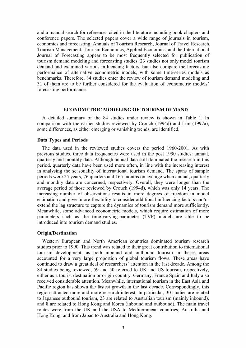
Data Types and Periods

The data used in the reviewed studies covers the period 1960-2001. As with

previous studies, three data frequencies were used in the post 1990 studies: annual,

quarterly and monthly data. Although annual data still dominated the research in this

period, quarterly data have been used more often, in line with the increasing interest

in analysing the seasonality of international tourism demand. The spans of sample

periods were 25 years, 76 quarters and 165 months on average when annual, quarterly

and monthly data are concerned, respectively. Overall, they were longer than the

average period of those reviewed by Crouch (1994d), which was only 14 years. The

increasing number of observations results in more degrees of freedom in model

estimation and gives more flexibility to consider additional influencing factors and/or

extend the lag structure to capture the dynamics of tourism demand more sufficiently.

Meanwhile, some advanced econometric models, which require estimation of more

parameters such as the time-varying-parameter (TVP) model, are able to be

introduced into tourism demand studies.

Origin/Destination

Western European and North American countries dominated tourism research

studies prior to 1990. This trend was related to their great contribution to international

tourism development, as both inbound and outbound tourism in theses areas

accounted for a very large proportion of global tourism flows. These areas have

continued to draw a great deal of researchers’ attention in the last decade. Among the

84 studies being reviewed, 59 and 50 referred to UK and US tourism, respectively,

either as a tourist destination or origin country. Germany, France Spain and Italy also

received considerable attention. Meanwhile, international tourism in the East Asia and

Pacific region has shown the fastest growth in the last decade. Correspondingly, this

region attracted more and more research interest. In particular, 30 studies are related

to Japanese outbound tourism, 23 are related to Australian tourism (mainly inbound),

and 8 are related to Hong Kong and Korea (inbound and outbound). The main travel

routes were from the UK and the USA to Mediterranean countries, Australia and

Hong Kong, and from Japan to Australia and Hong Kong.

4

TABLE 1

SUMMARY OF ECONOMETRIC STUDIES ON TOURISM DEMAND MODELING AND FORECASTING Legend: 1. Data frequency & period

A: annual

M: monthly

Q: quarterly

2. Region focused

I: inbound

O: outbound

3. Dependent variable

-B: on business

-H: for holidays

-VFR: visiting friends & relatives

BS: budget share of TE

EX: exports

IM: imports

ITC: No. of Inclusive tour chatters

NAC: No. of tourist accommodation

TA: tourist arrivals

TAHA: TA in hotels and apartments

TE: tourism receipts/expenditure

TM: tourism imports

TN: number of nights

TX: tourism exports

4. Independent variable

C: relative tourism price unadjusted by ER

Cd: tourism price in destination

Cir: tourism lifecycle

Co: tourism price in origin country

D: dummy variable

Dis: travel distance

DT: deterministic (linear) trend

ER: exchange rate

HR: average hotel rate

ICR: immigration crime rare

INF: capital stock in infrastructure

M4: monetary supply

ME: marketing expenditure

OEI: other economic indicators

P: population

PB: oil price per barrel

PI: price index

PREF: the preference index

RC: ER adjusted relative price

RPI: retail price index

SC: substitute price

SF: TC to substitute destinations

SM weighted TM

SPI: Stone’s price index

SS: stochastic seasonal component

ST: stochastic trend

TC: travel cost (airfare)

TS: travel cost by surface

TSS: TS to substitute destinations

TTM: total TM

Y: income in origin country

Yd: income in destination country

5 & 8 Main and alternative models

ADLM: autoregressive distributed lag

model

AR(I)MAX autoregressive (integrated)

moving average cause effect model

AR: autoregressive process

BNN: back-prorogation neural network

BSM: non-causal basic structural model

ES: exponential smoothing

FNN: Feed-forward neural network

GSR: Gradual switching regression

LCM: the learning curve model

MA: moving average

NLWSS: nonparametric locally

weighted scatterplot smoothing

SR: static regression

TFM: transfer function model

7. Estimation method 2(3)SLS: two (three)-stage least squares

CORN: Cochbrane-Crcutt procedure

DLS: dynamic least squares

GMM: generalized method of moments

KF Kalman filter algorithm

ML: maximum likelihood

NLLS: non-linear least squares

OLS: ordinary least squares

RIDG: ridge-trace procedure

SUR: seemingly unrelated regression

9. Diagnostic test reported

AC: autocorrelation test

ADF: augmented DF test

ARCH: autoregressive conditional

heteroscedasticity

BC-FF: Box-Cox functional form test

Chow1: structural stability test

Chow2: predictive failure test

CT: contingency table approach for

directional change error measures

CUSUM: cumulative sum of recursive

residual test for structural stability

CUSUMSQ: cumulative sum of squares

of recursive residuals

DF: Dickey-Fuller unit root test

DW: Durbin-Watson statistic

E(l): a statistic to check the goodness of fit

of models in the post-sample period

FU: Forecasting unbiasedness test

HEGY: Hylleberg, Engle, Granger and

Yoo test for seasonal and non-seasonal

unit roots

HESC: heteroscedasticity

HM: Henkiksson-Merton test for

directional change error measures

KPSS: Kwiatkowski-Phillips-Schmidt-

skin unit root test

LD- 2χ : a test for the inclusion of

lagged dependent variables and its

corresponding adjustment path

LM-AC: Lagrange-Multiplier test

MUCL: multicollinearity

Norm: test for non-normality

PEV: prediction error variance

PP: Phillips-Perron unite root test

Q-AC Box-Ljung Q-static

R: normalized correlation coefficient

RESET: mis-specification test

Z: acceptable output percentage (within

±15%)

5

Study

Frequency

& period 1

Region

Focused 2

Dependent

variable 3

Independent

Variable 4

Main

Model 5

Functional

form 6

Estimation

method 7

Alternative

Model 8

Diagnostic test

Reported 9

Akal (2004) A:

63-01 Turkey (I) TE TA AR(I)MAX

Linear/log-

linear ML SR DW DF Chow1 HESC

Akis (1998) A:

80-93 Turkey (I) TA Y RC SR Log-linear OLS DW

Ashworth &

Johnson (1990)

A:

72-86 UK (O and D) TE (H) Y P RPI D SR Log-linear OLS

DW homogeneity

stability

Bakkal (1991) A:

66-85 Germany (O) BS (of TN) TE/aggregated PI RC SC

Translog utility

function

Semi-log-

non-linear ML Homotheticity additivity

Cho (2001) Q:

75.1-97.4 Hong Kong (I) TA

ARIMA residuals of GDP

(GNP) CPI IM EX OEIs ARIMAX ARIMA ES

Crouch et al

(1992)

A:

70-88 Australia (I) TA/P Y/P RP TC ME D DT ADLM Log-linear OLS DW

De Mello et al

(2002)

A:

69-97

UK to France,

Portugal Spain BS TE/P/SPI RC SC D LAIDS

Semi-log-

linear SUR

DW Homogeneity

symmetry

Di Matteo (1999) Q:

79.1-95.4 Canada to US TE Y/P ER D SR Log-linear OLS NLWSS DW

Di Matteo & Di

Matteo (1993)

Q:

79.1-89.4 Canada to US TE Y/P ER RC-gas D ADLM Log-linear OLS DW

Divisekera

(2003) Not reported

UK US Japan

New Zealand (O) BS

TE/P/SPI average of RC+TC

SC D LAIDS

Semi-log-

linear SUR Homogeneity symmetry

Dritsakis (2004) A:

63-00

Germany and UK

to Greece TA Y/P C TC RC VAR(CI)/ECM Log-linear ML OLS

ADF DW LM-AC HESC

Chow1,2 RESET Norm

Dritsakis & Atha-

nasiadis (2000)

A:

60-93 Greece (I) TA/P

Y/P Cd SC ER ME DT D

investment ADLM Log-linear OLS CORN DW

Dritsakis & Papa-

nastasiou (1998)

A:

60-93 Greece (I) TA TE NAC

Cd DT TE NAC TA

investment

Simultaneous

equation model Log-linear 2SLS

DW LM-AC RESET

HESC Norm Theil-U

Durbarry &

Sinclair (2003)

A:

68-99

France to Italy

Spain UK BS TE/P/SPI RC SC D EC-LAIDS

Semi-log-

linear ML

DW Homogeneity

symmetry

Fujii et al (1985) A:

58-80 Hawaii (I)

BS on tourist

goods TE/P/SPI Cd DT SC LAIDS

Semi-log-

linear ML

Gallet & Braun

(2001)

A:

60-85 US (O) TA Y Cd /ER SC GSR Log-linear ML CORN

DW RESET Durbin h

LD- 2χ

Garía-Ferrer &

Queralt (1997)

M:

79.01-93.12 Spain (I) TE TA Y RC SC D STSM Log-linear

ARIMA STSM′ BSM

Q-AC

González &

Moral (1995)

M:

79.01-93.12 Spain (I) TE TA Y RC SC D STSM Log-linear KF ARIMA ECM TFM

r Q-AC HESC Norm

PEV E(l)

6

González &

Moral (1996)

M:

79.01-94.06 Spain (I) TE TA Y RC SC D STSM Log-linear KF ARIMA BSM TFM r Q-AC HESC Norm E(l)

Greenidge (2001) Q:

68.1-97.4 Barbados (I) TA Y RC SC ST SS Cir STSM Log-linear KF BSM DW Q-AC Norm HESC

Holmes (1997) M:

81.01-93.08

US to British

Columbia TA Y ER Cd Co D

Intervention &

TFM Log-linear OLS ARIMA Q-AC

Icoz et al (1998) A:

82-93 Turkey (I) TA

Cd ER No. of beds No. of

agents SR Log-linear OLS DW

Ismail et al

(2000)

M:

87.01-97.12 Japan to Guam TA Y ER TC D ADLM Linear OLS

Jensen (1998) A:

61(70)-95

Denmark (I)

TE Y RC SC D weather ADLM Log-linear OLS DW LM-AC DF

Jørgensen &

Solvoll (1996)

69-93

seasonal Norway (O) ITC

Y/P Price of ITC weather

OEI ADLM Log-linear OLS CORN DW

Kim & Song

(1998)

A:

62-94 Korea (I) TA Y TC TV RC D CI/ECM Log-linear OLS

Naive 1 SES MA

AR ARMA VAR

LM-AC CR DW Norm

HESC ARCH RESET

Chow2 Theil-U

Kim & Uysal

(1998)

M:

91.01-95.12

Hotels in Seoul,

Korea TN Cd TV No. of events ARMAX Log-linear

2SLS

CORN DW Q-AC

Kulendran (1996) Q:

75.3--95.2 Australia (I) TA Y RC TC D CI/ECM Log-linear ML

DW HEGY LM-AC Norm

RESET HESC Chow2

Kulendran &

King (1997)

Q:

75.1-94.4 Australia (I) TA Y RC TC D CI/ECM Log-linear ML

ARIMA STSM AR

AR(12) SR ARMA DW Theil-U

Kulendran &

Wilson (2000)

Q:

81.1-97.4 Australia (I) TA-B Y Yd TA-H TV/Yd RC IM D CI/ECM Log-linear ML OLS Naive 1 ARIMA ADF DW LM-AC HEGY

Kulendran &

Witt (2001)

Q:

78.1-95.3 UK (O) TA/P Y/P RC CS TC FS D

CI/ECM

ADLM Log-linear

ML

OLS Naive 1

DW LM-AC Chow2

HESC RESET

Kulendran &

Witt (2003a)

Q:

82.1-98.4 Australia (I) TA-B Y Yd TA-H TV/Yd C

ECM STSM

BSM Log-linear ML OLS

ARIMA1,4 ARIMA1

AR4Naive ADF DW Q-AC HESC

Kulendran &

Witt (2003b)

Q:

78.1-95.4 UK (O) TA-H Y RC ER C D TFM Log-linear OLS ML ECM ARIMA

DW LM-AC RESET

Chow2 HESC

Lanza et al

(2003)

A:

75-92

13 European

countries (O) BS

Total consumption/SPI Cd

SC D LAIDS

Semi-log-

linear SUR DF PP

Lathiras & Sirio

poulos (1998)

A:

60-95 Greece (I) TA/P Y/P RC SC ER D CI/ECM Log-linear ML

DW LM-AC RESET

HESC Theil-U CUSUM

CUSUMSQ Chow2 Norm

Law (2000) A:

66-96

Taiwan-Hong

Kong TA Y RC ER P ME HR BNN Non-linear

Naive 1 HES MA

FNN SR MAD MSE

7

Law & Au

(1999)

A:

77-97

Japan-Hong

Kong TA RC P ER ME HR FNN Linear Naive 1 SES MA SR Z r

Ledesma-Rodri-

guez et al (2001)

A:

79-97 Tenerife (I) TAHA Y/P ER ME INF PB ADLM Log-linear SUR OLS SR DW H-AC HESC

Lee et al (1996) A:

70-89 Korea (I) TE/P Y/P RC ER D SR Log-linear

OLS CORN

RIDG DW MUCL

Li et al (2002) A:

63/68-00 Thailand (I) TA Y RC SCD

ADLM VAR

CI/ECMs TVP Log-linear

KF

OLS ARIMA

ADF LM-AC HESC

Norm Chow1 RESET

Li et al (2004) A:

72-00 UK (O) BS TE/P/SPI RC SC D EC-LAIDS

Semi-log-

linear SUR Static LAIDS

DW PP DF Homogeneity

symmetry

Lim & McAleer

(2001)

Q:

75.1-96.4 Australia (I) TA Y/P TC ER C RC VAR CI/VECM Log-linear ML OLS

ADF HESC LM-AC

Norm Chow1,2

Lim & McAleer

(2002)

A:

75-96

Malaysia to

Australia TA Y/P TC ER C RC VAR CI/VECM Log-linear ML OLS ADLM

ADF LM-AC HESC

Norm Chow1,2

Lyssiotou (2001) Q:

79-91 UK (O) BS-H

TE-H/recreation-PI RC SC

D DT AIDS

Semi-log-

non-linear NLLS

Ac reset homogeneity

symmetry

Mangion et al

(2003)

A:

73-00

UK to Malta

Spain Cyprus BS TE/P/SPI RC SC EC-LAIDS

Semi-log-

linear SUR DW

Morley (1996) A:

72-92 Australia (I) TA-H Y/P TC SR Linear

OLS GMM

SUR DW Norm HESC

Morley (1997) A:

72-92 Australia (I)

TA-H TA-

VFR Y/P RC D TC ADLM Log-linear OLS RELF

Morley (1998) A:

72-92 Australia (I)

TA-H TA-

VFR Y/P RC TC D ADLM Non-linear ML

Morris et al

(1995)

Q:

81.1-93.4 Australia (I)

TA TA-H

TA-VFR RC TC ∆Y DT D SR Log-linear OLS CORN

LM-AC Norm

HESC RESET Chow2

O’Hagan &

Harrison (1984)

A:

64-81 US (O) BS TE/P/SPI RC SC D DT LAIDS

Semi-log-

linear SUR

DW HETE Homogeneity

symmetry

Papatheodorou

(1999)

A:

57-90

UK, Germany,

France (O) BS

TE/tourists/SPI RC SC D

DT LAIDS

Semi-log-

linear SUR DW

Payne & Mervar

(2002)

Q:

93.1-99.4 Croatia (I) TE Y RC D SR Log-linear OLS

DW LM-AC Norm

HESC RESET CUSUM

CUSUMSQ

Pyo et al (1991) A:

72-87 US domestic

TE on tourist

goods TE/SPI Cd SC LES

Semi-log-

linear SUR OLS

Qiu & Zhang

(1995)

A:

75-90 Canada (I) TA TE Y/P ER Cd D DT ICR SR Linear OLS log-linear SR BC-FF

Qu & Lam

(1997)

A:

84-95

Mainland China

to Hong Kong TA Y/P C ER D SR Linear OLS DW MUCL

8

Riddington

(1999)

A:

73-94 UK Skiing place TA M4 DT TVP Linear KF

LCM Static

regression DW

Rosselló-Nadal

(2001)

M:

75.01-99.12

Balearic Islands

(I) TA ER RC OEIs

ADLM(Leading

indicator) Linear OLS Naive1 ARIMA

DW Q-AC LM-AC AIC

SC

Rosselló-Nadal et

al (2004)

M/A:

82-01

The Balearic

Islands (I)

Gini-

coefficient Y/P ER RC ECM Linear DLS DW LM-AC AIC SC

Shan & Wilson

(2001)

M:

87.01-98.01 China (I)

TA Y RC

IM+EX ER TA Y RC IM+EX ER VAR Linear SUR

ADF Modified Wald AIC

SC

Sheldon (1993) A:

70-86 US (I) TE Y ER RC SC SR

Linear/log-

linear OLS

Naïve1,2 Trend

fitting models

Smeral et al

(1992)

A:

75-00

18 OECD

countries (I/O)

TM

TX

Y Co D

TTX RC D (ST)

complete

system linear DW

Smeral & Weber

(2000)

A:

75-96

20 OECD

countries (I/O)

TM

TX

Y RC D (DT)

SM RC D (DT)

complete

system linear OLS DW

Smeral & Witt

(1996)

A:

75-94

18 OECD

countries (I/O)

TM

TX

Y Co D

SM RC D

complete

system Linear

OLS

Sauss-Seidel DW

Song et al (2000) A:

65-94 UK (O) TA/P-H Y/P RC SC PREF D CI/ECM Log-linear OLS

Naive 1 MA AR

ARMA VAR

ADF PP Norm ARCH

DW LM-AC RESET

HESC Chow2

Song, Witt & Li

(2003)

A:

63/68-00 Thailand (I) TA Y RC SC D

ADLM VAR

CI/ECMs TVP Log-linear

KF

OLS ARIMA Naive 1

ADF LM-AC HESC

Norm Chow1 RESET

Song, Witt &

Jensen (2003)

A:

69-97 Denmark (I) TA/P-H TE/P RC SC TC DT D CI/ECM Log-linear OLS

SR Naive 1 ARIMA

VAR ADLM TVP

LM-AC Norm HESC

RESET Chow1

Song & Witt

(2003)

A:

62-98 Korea (I) TA Y TV RC SC D ADLM ECM Log-linear OLS

LM-AC Norm HESC

RESET

Song & Wong

(2003)

A:

73-00

Hong Kong (I)

TA Y RC SC TVP Log-linear KF AIC SC LL

Song, Wong &

Chon (2003)

A:

73(81)-00 Hong Kong (I) TA Y RC SC D ADLM Log-linear OLS

LM-AC Norm

HESC RESET Chow2

Syriopoulos

(1995)

A:

62-87

Mediterranean

countries (I) TE Y/P C RC ER D DT(ST) CI/ECM Log-linear OLS

LM-AC ARCH HESC

Chow1

Syriopoulos &

Sinclair (1993)

A:

60-87

US UK Germany

France Sweden (O) BS TE/P/SPI RC SC D DT LAIDS

Semi-log-

linear OLS SUR

DW Homogeneity

symmetry

Turner et al

(1998)

Q:

78.1-95.4 UK (O)

TA-B TA-H

TA-VFR

Y/C RC SC TC SF IM EX

OEIs

Structural

equation model Linear MUCL

Turner & Witt

(2001a)

Q:

78.1-97.4 New Zealand (I)

TA-B TA-H

TA-VFR

Y P RC TC SFTV/Yd IM

EX, OEIs

Structural

equation model Linear MUC

Turner & Witt

(2001b)

Q:

78.2-98.3

New Zealand (I)

TA TA-B TA-

H TA-VFR Y RC TC TV/Yd STSM Log-linear KF BSM Norm HESC DW Q-AC r

9

Uysal & Roubi

(1999)

Q :

81.1-96.4 Canada to US TE Y/P RC D ADLM Log-linear OLS FNN

Vanegas & Croes

(2000)

A:

75-96 US to Aruba TA Y RC ER ADLM Log-linear OLS Linear DW predictive efficiency

Var & Icoz

(1990)

A:

79-87 Turkey (I) TA Y/P ER Dis SR Log-linear OLS

Vogt & Wittaya-

korn (1998)

A:

60-93 Thailand (I) TE RC ER Y CI/ECM Log-linear OLS ADF

Webber (2001) Q:

83.1-97.4 Australia (O) TA

Y RC Cd/ER (C ER) ER-

volatility CI/VAR Log-linear OLS ADF PP symmetry

White(1985) A:

54-81 US (O) BS TE/P/SPI RC TC SC D DT LAIDS

Semi-log-

linear ML Homogeneity symmetry

Witt et al (2003) A:

69-97 Denmark (I) TA/P-H TE/P RC SC TC DT D CI/ECM Log-linear OLS

Naive 1 ARIMA SR

VAR ADLM TVP FU HM CT

Witt & Witt

(1990)

A:

65-80

European

countries, US (I/O) TA/P

Y/P Cd SC ER TC SF TS

TSS D DT SR Log-linear OLS CORN DW MSPE

Witt & Witt

(1991)

A:

65-85

France, Germany,

UK, US (O) TA/P TA

Y/P C SC ER, TC SF TS

TSS D SR Log-linear OLS Time series models

Witt & Witt

(1992)

A:

65-80

France Germany

UK US (O) TA/P Y/P Cd CS ER TC SF D ADLM Log-linear OLS CORN

Naive 1,2 AR ES

ARIMA Trends DW

10

Measures of Tourism Demand

Compared to tourism demand studies prior to 1990, the measures of tourism

demand have not changed much. Tourist arrivals was still the most common measure

in the last decade, followed by the tourist expenditure. In particular, tourist

expenditure, in the form of either absolute values or budget shares, is required by the

specification of demand system models, such as the linear expenditure system (LES)

and the AIDS.

Compared with the tourism literature before 1990, recent studies pay more attention

to disaggregated tourism markets by travel purpose (for example, Morley 1998;

Turner et al 1998; Turner and Witt 2001a). Amongst various market segments, leisure

tourism attracted the most research attention. 12 studies focused on this particular

tourism market (for example, Ashworth and Johnson 1990; Kulendran and Witt 2003b;

Song, Romilly, and Liu 2000; Song, Witt, and Li 2003). Different market segments

are associated with different influencing factors and varying decision-making

processes. Therefore, studies at disaggregated levels give more precise insights into

the features of the particular market segments. As a result, more specific and accurate

information can be provided to develop efficient marketing strategies.

Explanatory Variables

Consistent with previous tourism demand studies, income, relative prices, substitute

prices, travel costs, exchange rates, dummies and deterministic trends were the most

frequently considered influencing factors in the reviewed studies. In spite of different

definitions of income and relative prices, both of them were shown to be the most

significant determinants for international tourism demand. Although travel costs had

been considered in over 50% of the studies reviewed by both Crouch and Lim, in

recent studies they did not attract as much attention as before, with only 24 studies

including this variable. As precise measurements of travel costs were lacking,

especially of the aggregate level, proxies such as airfares between the origin and the

destination had to be used. However, only in a few cases did the use of proxies result

in significant coefficient estimates. Another reason for insignificant effects of travel

costs may be related to all inclusive tours where charter flights are often used, and

hence airfares bear little relation to published scheduled fares. The deterministic trend

variable describes a steady change format, which is too restrictive to be realistic and

may cause serious multicollinearity problems. With this borne in mind, recent studies

have been less keen to include it in model specifications. This variable only appeared

in 11 reviewed studies. To capture the effects of one-off events, dummy variables

have been commonly used. The two oil crises in the 1970s were shown to have the

most significant adverse impacts on international tourism demand, followed by the

Gulf War in the early 1990s, and the global economic recession in the mid 1980s.

Other regional events and origin/destination-specific affairs have also been taken into

account in specific studies.

It should be noted that no effort has been made to examine the impact of tourism

supply in the tourism demand literature, which means that the problem of

identification has been ignored. An implicit assumption of this omission is that the

tourism sector concerned is assumed to be sufficiently small and the supply elasticity

is infinite. To draw more robust conclusions with regard to demand elasticity analysis,

however, this condition needs to be carefully examined in future studies.

11

Functional Forms

Continuing the trend of the 1960s-1980s, log-linear regression was still the

predominant functional form in the context of tourism demand studies in the 1990s.

53 studies specified log-linear models, 17 linear models, and only 3 non-linear forms.

In addition, a semi-log (both linear and non-linear) form appeared in 14 demand

systems, principally AIDS models, where only independent variables (prices and real

expenditure) were transformed into logarithm. Crouch (1992) concluded that the log-

linear form was generally proved to be superior when both linear and log-linear forms

were tested. In a recent study, Vanegas and Croes (2000) compared a few linear and

log-linear models of US demand for tourism in Aruba and concluded that log-linear

models generally fitted the data better (although only slightly) in terms of the

statistical significance of the estimated coefficients, whereas Qiu and Zhang (1995)

ran a similar comparison but did not find a significant difference between the two

forms.

An advantage of using log-linear regressions is that the log transformation may

reduce the integration order of the variables from I(2) to I(1), so that the standard

cointegration (CI) analysis is allowed. However, the elasticities derived from log-

linear regressions (within the traditional fixed-parameter framework) are constant

over time. This condition is quite restrictive and often leads to the failure of dynamic

analysis of tourism demand. Moreover, such a model may not be useful for short-term

forecasting (Lim 1997b). However, the problem of constant elasticities can be solved

by rewriting the regression in the state space form (SSF) and estimating it by the

Kalman filter algorithm. Such a method is termed the TVP model, and it will be

introduced in the following section.

Model Specification and Estimation

CI Model and Error Correction Model (ECM). In the early 1990s, econometric

modeling and forecasting of tourism demand was still restricted to static models,

which suffer from quite a few problems such as spurious regression (Song and Witt,

2000). Since the mid 1990s, dynamic models, for example, a number of specific forms

of the autoregressive distributed lag models (ADLMs), (Hendry 1995, p. 232)

including ECMs have appeared in the tourism demand literature. The potentially

spurious regression problem can be readily overcome by using the CI/ECM analysis.

When the CI relationship is identified, the CI equation can be transformed into an

ECM (and vice versa), in which both the long-run equilibrium relationship and short-

run dynamics are traced. An additional advantage of using the ECM is that the

regressors in an ECM are almost orthogonal and this avoids the occurrence of

multicollinearity, which may otherwise be a serious problem in econometric analysis

(Syriopoulos, 1995). However, it should be noted the CI relationship does not

necessarily hold in every case of tourism demand. The application of this

methodology should be subject to strict statistical tests.

17 of the studies under review applied the CI/ECM technique to international

tourism demand analysis. Four CI/ECM estimation methods have been used - the

Engle-Granger (1987) two-stage approach (EG), the Wickens-Breusch (1988) one-

stage approach (WB), the ADLM approach (Pesaran and Shin, 1995), and the most

frequently employed Johansen (1988) maximum likelihood (JML) approach. Due to

12

different modeling strategies, these models may yield demand elasticities with large

discrepancies for the same data set. Moreover, unlike the other methods, the JML

approach may detect more than one CI relationship amongst the demand and

explanatory variables. The determination of the unique CI relationships in the JML

framework involves testing for identification. It is important to impose appropriate

identifying restrictions, which should have an explicit underpinning of economic

theories (Harris and Sollis 2003). All of these approaches have their merits, and there

has not been clear-cut evidence to show that any one is superior to the others.

Sometimes the evaluation is associated with their ex post forecasting performance.

Time Varying Parameter (TVP) Model. To overcome the unrealistic assumption of

constant coefficients (or elasticities in log-linear regression) associated with the

traditional econometric techniques, the TVP model was developed and has been

applied in tourism demand studies. The TVP model is specified in the following SSF:

tttt xy εα += (1)

ttttt RT ηαα +=+1 (2)

where ty is a vector of tourism demand, tx is an matrix of explanatory variables, tα

is an unobserved vector of parameters known as the state vector, tT and tR are

transition matrices, and tε and tη are vectors of Gaussian disturbances which are

serially independent and independent of each other at all time points. The TVP model

can be estimated using the Kalman filter algorithm. The TVP model first appeared in

the tourism literature in 1999 and only 6 applications have been identified. They were

all related to annual tourism data and the main focus of these studies was the

evolution of demand elasticities over a relatively long period. Taking sufficient

account of the dynamics of tourist behaviors, the TVP model is likely to generate

more accurate forecasts of tourism demand. This will be discussed in a later section.

Vector Autoregressive (VAR) Approach. Most of the traditional tourism demand

models are specified in a single-equation form, which implicitly assumes that the

explanatory variables are exogenous. If the assumption is invalid, the estimated

parameters are likely to be biased and inconsistent. Where exogeneity is not assured,

the vector autoregressive (VAR) model is more appropriate. The VAR model is a

system of equations in which all variables are treated as endogenous. It can be written

as:

∑=

− ++=p

i

ttitit UBZYAY1

(3)

where tY is a k vector of endogenous variables, tZ is a d vector of exogenous

variables, Ai and B are matrices of coefficients to be estimated, and tU is a vector of

innovations that is independently and identically distributed. The JML CI/ECM

analysis is based on the unrestricted VAR method. Since 1998, there have been 8

studies utilizing the VAR approach including the cointegrated VAR and VECM for

tourism demand analysis.

Almost Ideal Demand Systems (AIDS). Another limitation of the single-equation

analysis of tourism demand is that this approach is incapable of analyzing the

interdependence of budget allocations to different tourist products/destinations.

13

Lacking a strong underpinning of economic theory, the single-equation approach is

relatively ad hoc. As a result, it is hard to attach a strong degree of confidence to the

results (especially regarding demand elasticities) derived from this methodology. On

the contrary, the demand system approach, which embodies the principles of demand

theory, is more appropriate for tourism demand analysis. Amongst a number of

system approaches available, the AIDS introduced by Deaton and Muellbauer (1980)

has been the most commonly used method because of its considerable advantages

over others. The AIDS model is specified in the form:

i

j

ijijii uPxbpw +++= ∑ )/log(logγα (4)

where wi is the budget share of the ith good, pi is the price of the ith good, x is total

expenditure on all goods in the system, P is the aggregate price index for the system,

and ui is the disturbance term. The aggregate price index P is defined as:

∑ ∑∑++=i i j

jiijii pppaP loglog2

1loglog 0 γα (5)

where 0a and iα are parameters that to be estimated. Replacing P with the following

Stone’s (1954) price index (P*), the linearly approximated AIDS is derived and

termed “LAIDS”.

∑=i

ii pwP log*log (6)

The AIDS/LAIDS can be used to test the properties of homogeneity and symmetry

associated with demand theory. Moreover, both uncompensated and compensated

demand elasticities including expenditure, own-price and cross-price elasticities can

be calculated. They have a stronger theoretical basis than the single-equation

approach.

The LAIDS model can be estimated by three methods: ordinary least squares (OLS),

maximum likelihood (ML) and Zellner’s (1962) iterative approach for seemingly

unrelated regression (SUR) estimation. The SUR method is used most often, as it

performs more efficiently than OLS in the system with the symmetry restriction

(Syriopoulos 1995). It will also converge to the ML estimator, provided that the

residuals are distributed normally (Rickertsen 1998).

Since the AIDS model was introduced into tourism demand studies in the 1980s, it

has not attracted much attention until recently. 12 applications have been identified

including 3 in the 1980s, 1 in 1993 and 8 after 1999. Most of these studies analyzed

allocations of tourists’ expenditure in a group of destination countries, while Fujii et

al (1985) investigated tourists’ expenditure on different consumer goods in a

particular destination. Where a group of destinations are concerned, substitutability

and complementarity between them are investigated by calculating cross-price

elasticities. The AIDS/LAIDS has been developed from the original static form to the

error correction form. Combing the ECM with the LAIDS, Durbarry and Sinclair

(2003), Li, Song, and Witt (2004), and Mangion, Durbarry, and Sinclair (2003)

specified EC-LAIDS models to examine the dynamics of tourists’ consumption

behavior.

14

Other demand system models such as the LES by Pyo, Uysal, and McLellan (1991)

and the translog utility function by Bakkal (1991) have also appeared in the tourism

context, but compared to AIDS/LAIDS their applications were extremely rare.

Time Series Models Augmented with Explanatory Variables. Another emerging

trend of tourism demand research has been the introduction of the advanced time-

series techniques into the causal regression framework. By doing so, the advantages

of both methodologies are combined. Two notable examples are the structural time

series model with explanatory variables (STSM) which expands the basic structural

model without explanatory variables (BSM), and the AR(I)MAX model based on the

AR(I)MA technique. The BSM and the AR(I)MA model are advanced time-series

forecasting techniques and have shown favorable forecasting performance in the

tourism context. The BSM can readily capture the trends, seasonal patterns and cycles

involved in demand variables. Similar to the technique of the TVP model, the BSM

and STSM are also written in the SSF and estimated by the Kalman filter. They are

very useful as far as seasonal data are concerned. The AR(I)MA model includes both

autoregressive filters and moving average filters to account for systematic effects and

shock effects in the endogenous variable itself, respectively. With explanatory

variables being added into the model specifications, the STSM and the AR(I)MAX

model are more powerful in interpreting variations in demand variables relative to the

BSM and the AR(I)MA model, respectively. Meanwhile, they embody the dynamics

of the demand variables and overcome the problem of autocorrelation suffered by

conventional static regressions. Amongst the 84 econometric studies, there are 6

applications of the STSM and 3 of the AR(I)MAX model. Another advantage of using

these models is the potential to generate accurate tourism forecasts, which will be

investigated in a later section.

Data frequency affects the specification of the models. For example, the STSM and

AR(I)MAX models have been used more often when monthly or quarterly data are

concerned. Annual data, however, have always been used in the estimation of the

AIDS/LAIDS models. Annual data, however, have always been used in the estimation

of AIDS/LAIDS models. The main reason for this is that these latter models aim to

examine long-run demand elasticities. In most cases, the TVP model has been applied

to annual data, although it is possible to incorporate seasonality into the specification.

The combination of the TVP model with the STSM is of interest for future tourism

demand studies. Depending on the integration order of the data, the ECM and VAR

models can readily accommodate data with different frequencies (Song and Witt

2000).

Diagnostic Tests

Witt and Witt (1995) pointed out the problems in tourism demand models prior to

the early 1990s, one of which is the lack of diagnostic checking. As a result, the

inferences from the estimated models might be highly sensitive to the statistical

assumptions, especially when a small number of observations are available (Lim

1997a). The situation has changed since the mid 1990s. In addition to the

conventional statistics reported in earlier studies such as goodness of fit, F statistic

and Durbin-Watson autocorrelation statistic, many recent studies have carried out

tests for unit roots, higher-order autocorrelation, heteroscedasticity, non-normality,

mis-specification, structural break and forecasting failure. In particular, Dristakis

(2003), Kim and Song (1998), and Song, Romilly, and Liu (2000) each reported about

15

10 diagnostic tests for their estimates. Amongst various diagnostic tests, unit root tests

for annual data or seasonal unit root tests for monthly or quarterly data have been

widely used where CI/ECM approaches were considered. Most of the models reported

in the studies after 1995 passed the majority of these tests. The enhanced model

performance is likely to generate more accurate forecasts and more meaningful

implications for the practical operations of tourism industries and government

agencies.

Demand Elasticities

Tourism demand elasticities have been discussed comprehensively by Crouch

(1992, 1994a, 994b, 1995, 1996). Consistent with his findings, recent studies have

also shown that the income elasticity is generally greater than one, indicating that

international tourism, especially long-haul travel, is a luxury. The own-price elasticity

is normally negative, although the magnitudes vary considerably. The reasons that

cause the discrepancies in demand elasticities have been identified in Crouch’s work,

therefore this paper will only address some additional issues.

Long-Run and Short-Run Elasticities. In addition to the findings in line with

previous studies, some new light has been shed on the literature by the research

adopting the CI/ECM techniques. Given the CI relationship being assured by

statistical tests, long-run and short-run tourism demand elasticities can be calculated

from the CI equation and the ECM, respectively. With regard to the income elasticity,

lower degrees of significance in ECMs than those in the CI models indicate that

income affects tourism demand more in the long run than in the short run. To some

extent, it indicates that Friedman’s (1957) permanent income hypothesis holds. In

other words, consumption depends on what people expect to earn over a considerable

period of time, and fluctuations in income regarded as temporary have little effect on

their consumption spending. Many empirical studies also show that the values of both

the income and own-price elasticities in the long run are greater than their short-run

counterparts, suggesting that tourists are more sensitive to income/price changes in

the long run than in the short run. These findings are in line with demand theory. Due

to information asymmetry and relatively inflexible budget allocations, it takes time

before income changes affect tourism demand (Syriopoulos 1995).

Cross-Price Elasticities. The cross-price elasticity contributes to the analysis of the

interrelationships between alternative destinations. As mentioned earlier, this is one of

the advantages of the AIDS model over single-equation regressions. Seven studies

used this approach to study UK outbound tourism demand. Table 2 summarizes the

substitution and complementarity relationships between alternative destinations

considered by UK tourists. Due to the differences with respect to the composition of

the demand systems, the data periods, the definitions of variables and estimation

methods, some contradictions between the findings are identified. However, some

findings are supported across studies. For example, a significant substitution effect

between France and Spain was commonly found (see De Mello, Park and Sinclair

2002, Li, Song, and Witt 2004, Lyssiotou 2001), and Greece and Italy were generally

regarded as complementary destinations by UK tourists (see Li, Song, and Witt 2004,

Lyssiotou 2001, Papatheodorou 1999, Syriopoulos and Sinclair 1993). Moreover,

Italy and Turkey were substitutes for each other to some extent (see Papatheodorou

1999, Syriopoulos and Sinclair 1993). These findings have important policy

implications for the destination concerned. A significant substitution effect indicates

16

strong competitors, and different degrees of substitution (suggested by the values of

the elasticities abε and baε ) between the competing destinations a and b show their

competitive positions in the tourism markets. Therefore, the implication could be to

adopt appropriate strategies based on the specific attributes the destinations possess or

to focus on differentiated markets segments, i.e., to make full use of their competitive

advantages. Where complementary effects are in place, the destinations involved may

consider launching joint marketing programs to maximize their total profits.

Evolution of Eelasticities. Compared to the long-run constant demand elasticities,

analyzing the evolution of demand elasticities over time has great importance for

short-term forecasting. Crouch (1994b, 1996) has identified the differences regarding

income and own-price elasticities in different time periods. Using the TVP approach,

Li, Song, and Witt (2002), Song and Witt (2000), and Song and Wong (2003)

confirmed the above findings in their empirical studies. In particular, the significant

impacts of the two oil crises in the 1970s and the economic recession in the 1980s on

tourism demand, in terms of the income elasticities, were readily accommodated in

their models. It suggests that the TVP model is preferable to the log-linear fixed-

parameter regressions when investigating the dynamics of tourism demand.

PERFORMANCE OF FORECASTING MODELS

Among the 84 studies being reviewed, 23 papers exercised the compared

forecasting performance amongst different econometric models or amongst

econometric, univariate time-series and other (e.g. neural network) models. Apart

from Rossello-Nadal (2001) who investigated forecasting models’ turning point

accuracy, all the other papers examined forecast error magnitudes. Therefore, the

review of forecasting models’ performance will focus on error magnitude accuracy. In

addition to error magnitudes, Witt, Song, and Louvieris (2003) also observed

directional changes of demand forecasts, and Witt and Witt (1991) and its extended

version Witt and Witt (1992) included directional changes and trend changes in their

forecasting accuracy evaluations. Due to extremely small numbers of applications,

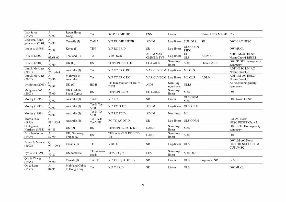
these two measures of forecasting accuracy are ignored in this review. The ranks of

compared models in each of the 22 studies1, in terms of forecast accuracy, are

tabulated for detailed analysis (Table 3). Since error magnitude accuracy dominates

the evaluation of tourism demand forecasting, the following discussion will mainly

focus on this measure.

Table 3 summarizes the rankings of forecasting models measured by the MAPE

except for 4 studies in which only the MAE or RMSE was available. Due to space

limitations, the results of other measures are omitted from this table. The rankings of

competing models at each forecasting horizon and the overall ranks are presented in

Table 3. Where they were not reported directly in the original papers, the aggregation

of MAPEs is calculated based on the individual MAPEs originally reported.

1 Li, Song, and Witt (2004) is excluded from Table 2 due to different models considered in the

comparison.

17

TABLE 2

INTERRELATIONSHIPS BETWEEN ALTERNATIVE DESTINATIONS WITH REGARD TO UK TOURISTS

France Cyprus Greece Italy Malta Portugal Spain Turkey Yugoslavia Australia New Zealand Canada US

France -D C C’ -D -C C’ A D C -C’ A D C C’ -D -D

Cyprus E E

Greece -D C C’ -G -F -D -C -C’ G F -D -C C’ G F -D C -C’ -G F -F D D

Italy -D -C C’ -G -D -F -C -C’ -G F -D C C’ G F -D -C C’ F G -F D D

Malta -E E

Portugal A C C’ D G -C C’ -D F F -G C C’-D -C G F A -C -C’ -D -G F -F D D

Spain A C C’ D E F G C -C’ -D F G -C C’ -D E G A -C -C’ -D F -G F F D D

Turkey F -G F G F -G F -G -F

Yugoslavia -F -F -F -F

Australia B B

New Zealand B B

Canada -D D D D D -D

US -D D D D D B B -D

Notes: 1. Legend: A: De Mello, Park, and Sinclair (2002); B: Divisekera (2003); C: Li, Song, and Witt (2004) C΄ represents short-run elasticities; D: Lyssiotou (2001) some

destinations are groups. In these cases, the relationships between groups are regarded to apply to the individual countries in these groups; E: Mangion, Durbarry,

and Sinclair (2003); F: Papatheodorou (1999); G: Syriopoulos and Sinclair (1993).

2. Negative signs stand for complementary effects, where no sign is given, the substitute effect is detected. The letters in bold refer to statistically significant effects. G

did not report the significance level.

3. Cross-price elasticities in A, D, E and F refer to uncompensated elasticities, while those in B, C and G refer to compensated elasticities.

18

TABLE 3

RANKINGS OF FORECASTING ACCURACY COMPARISON

Study

Dat

a

Fre

quen

cy

Nai

ve

1

Nai

ve

2

Lin

ear

Tre

nd

Non-l

inea

r

Tre

nd

Gom

per

tz

Sim

ple

ES

D

ouble

ES

MA

AR

1

AR

12

AR

(I)M

A

SA

RIM

A

AR

(I)M

AX

LC

M

TF

M

FN

N

BN

N

BS

M

ST

SM

SR

AD

LM

AD

LM

-EC

M

WB

-EC

M

EG

-EC

M

JML

-EC

M

VA

R

TV

P

Err

or

Mea

sure

Bes

t

Model

Akal (2004) A MAPE

Overall 1 2 ARMAX

Cho (2001) Q MAPE

1-8 steps ahead 3 4 1 2 SARIMA

González & Moral (1995) M RMSE

1 step ahead 3 1 2 4 TFM

González & Moral (1996) M RMSE

1 step ahead 3 2 1 STSM

Kim & Song (1998) A MAE

3 steps ahead 6 4 5 3 1 2 7

5 steps ahead 7 5 6 4 1 3 2

7 steps ahead 7 5 6 3 2 1 4

10 steps ahead 6 4 5 3 1 2 7

Overall 7 4 5 3 1 2 6 ARMA

Kulendran & King (1997) Q MAPE

1 step ahead 3 5 3 1 2 6

2 steps ahead 3 6 3 1 2 3



Overall 2 6 3 1 4 5 SARIMA

Kulendran & Wilson (2000) Q MAPE

1step ahead 2 3 1 EG-ECM

Law (2000) A MAPE

1 step ahead 3 2 4 5 1 6 BNN

Kulendran & Witt (2001) Q MAPE

1 step ahead 3 5 1 2 4

2 steps ahead 1 5 3 2 4



Overall 1 5 4 2 3 Naïve 1

Kulendran & Witt (2003a) Q MAPE

1 step ahead 6 5 1 7 2 4 3

19

4 steps ahead 1 5 4 7 3 6 2

6 steps ahead 1 4 3 7 2 6 5

Overall 1 4 3 7 2 6 5 Naïve 1

Kulendran & Witt (2003b) Q MAPE

1 step ahead 1 2 3

2 steps ahead 2 1 3

4 steps ahead 1 3 2

8 steps ahead 2 3 1

Overall 2 3 1 JML-ECM

Law & Au (1999) A MAPE

1 step ahead 2 4 5 1 3 FNN

Li et al (2002) A MAPE

1 step ahead 6 5 9 7 8 4 1 3 2

2 steps ahead 5 7 9 4 8 3 2 6 1

3 steps ahead 6 2 3 4 8 5 7 8 1

4 steps ahead 6 2 5 3 9 4 7 9 1

5 steps ahead 7 5 6 2 4 3 8 9 1

Overall 5 4 8 3 7 2 6 9 1 TVP

Riddington (1999) MAPE

1 step ahead 3 2 1 TVP

Sheldon (1993) A MAPE

1-6 steps ahead * 1 3 4 7/5 2 8/6 Naïve 1

Song et al (2000) A MAE

1 step ahead 5 3 4 1 2 EG-ECM

Song et al (2003b) A MAPE

1 step ahead 4 6 2 3 5 8 7 1

2 steps ahead 3 7 1 4 5 8 6 2

3 steps ahead 4 7 1 6 5 8 3 2

4 steps ahead 3 7 1 6 5 8 2 4

Overall 3 7 1 6 5 8 4 2 SR

Song & Witt (2000) A MAPE

1 step ahead 3 4 5 5 2 7 1

2 steps ahead 1 6 4 5 2 7 3

1 to 4 steps ahead 2 3 4 6 5 7 1 TVP

Turner & Witt (2001a) Q MAPE

1 step ahead 2 1

4 steps ahead 2 1

8 steps ahead 2 1

Overall 2 1 STSM

Witt et al (2003) A MAPE

20

1 step ahead 3 4 5 1 6 8 7 2

2 steps ahead 3 4 7 2 5 8 1 6

3 steps ahead 3 4 5 2 7 8 1 6

Overall 3 4 6 1 7 8 2 5 ADLM

Witt & Witt (1991,1992) A MAPE

1 year ahead 1 4 7 6 2 3 5

2 years ahead 2 7 6 5 3 1 4

Overall 2 5 7 6 3 1 4 AR1

Note: * 7/5 refer to the ranks of log quadratic and exponential trend fitting models, respectively, and 8/6 refer to linear and log-linear regressions, respectively.

TABLE 4

DESCRIPTIVE STATISTICS OF RANKINGS IN TABLE 3

Nai

ve

1

Nai

ve

2

Lin

ear

Tre

nd

Non-l

inea

r

Tre

nd

Gom

per

tz

Sim

ple

ES

Double

ES

MA

AR

1

AR

12

AR

(I)M

A

SA

RIM

A

AR

(I)M

AX

LC

M

TF

M

FN

N

BN

N

BS

M

ST

SM

SR

AD

LM

AD

LM

-EC

M

WB

-EC

M

EG

-EC

M

JML

-EC

M

VA

R

TV

P

No of studies 14 2 1 2 1 4 3 3 5 1 8 8 2 1 2 2 1 1 6 8 4 1 4 4 9 6 5

Mean of overall ranks 2.8 4.0 4.0 5.0 6.0 3.5 2.7 4.7 2.6 6.0 3.9 2.9 1.5 3.0 2.0 3.0 1.0 2.0 2.7 4.0 3.3 7.0 4.5 3.0 4.8 5.0 2.0

Standard deviation 1.8 1.4 2.8 0.6 1.2 0.6 1.1 1.7 2.0 0.7 1.4 2.8 2.0 2.4 2.1 2.1 2.4 2.4 2.8 1.7

Frequency of top 2 models

1 step ahead 4/12 0/1 0/2 0/1 1/2 1/1 0/2 0/4 0/1 1/7 4/7 0/1 2/2 1/2 1/1 1/1 5/6 2/7 3/4 0/1 0/4 2/4 2/8 1/5 5/5

2 steps ahead 2/6 0/1 0/1 0/1 0/1 1/2 0/1 0/5 2/3 1/1 2/2 1/4 1/4 0/1 0/4 0/1 2/7 1/4 2/4

3 steps ahead 0/4 0/1 0/1 0/1 2/4 1/3 1/3 0/1 0/3 1/4 1/4 2/3

4 steps ahead 3/5 1/1 0/1 1/5 2/4 0/1 0/1 2/4 0/2 0/2 0/1 0/2 2/6 1/2 1/2

5 steps ahead 0/2 0/1 0/1 0/1 1/2 0/1 1/1 0/1 0/1 0/2 1/2 1/1

6 steps ahead 1/1 0/1 0/1 0/1 1/1 0/1 0/1

7 steps ahead 0/1 0/1 0/1 0/1 1/1 1/1 0/1

8 steps ahead 2/2 1/1 0/1 1/2 1/3 0/1 1/3 1/3

10 steps ahead 0/1 0/1 0/1 0/1 1/1 1/1 0/1

Total 12/34 0/2 0/3 0/2 1/7 1/1 0/6 3/13 0/4 9/28 9/18 0/1 3/5 1/2 1/1 2/3 10/16 4/17 6/14 0/5 0/14 2/5 10/33 5/19 11/15

21

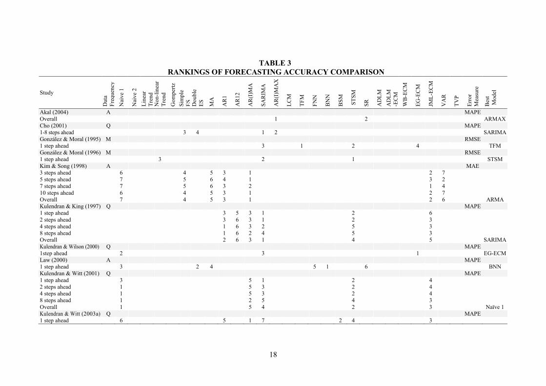
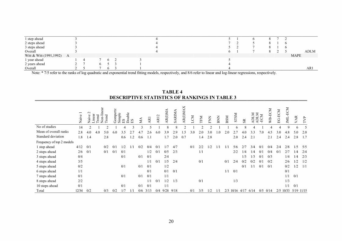
Overall Performance of Forecasting Models

Based on the rankings shown in Table 3, Table 4 provides some descriptive

statistics. In the forecasting performance comparison, the naïve 1 model, which is also

known as “no change” model, is often used as a benchmark. Various ECMs,

especially the JML-ECM, are most often considered in the econometric forecasting of

tourism demand. The static regression model also frequently appeared in the

comparison as either a benchmark for econometric models or a competitor for time-

series models. Within the time-series forecasting scope, AR(I)MA models, including

the seasonal version SAR(I)MA, has been the most popular.

The frequency with which each model appeared in the top two positions across all

forecasting horizons suggests that the TVP model and the STSM, based on the same

modeling technique, both performed relatively well in general. In particular, the TVP

model was ranked number one in 7 and number two in 4 out of 15 cases. These

findings are confirmed by the calculated means of overall ranks in all studies. On the

other hand, the standard deviation of the overall ranks shows that the VAR model

performed the least consistently, and its ranks varied from the top to the bottom. It

should be noted that, due to the small number of studies being reviewed, some caution

should be given to the interpretation of the means and standard deviations of the

overall ranks.

Factors Influencing Relative Forecasting Performance

Tables 3 and 4 show that there is no one forecasting model that outperforms the

others in all situations. Various factors are attributed to the discrepancies in

performance between the studies.

Measures of Forecasting Error Magnitudes. Different measures for forecasting error

magnitudes have been available for tourism demand forecasting evaluations. The

predominant measure was MAPE, commonly used in all studies with only 4

exceptions and 144 out of 180 individual comparisons (from original papers). It was

followed by RMSE and RMSPE, and they were used in 97 and 86 comparisons,

respectively. In very few studies, other evaluation measures were applied, such as

MAE and Theil’s U statistic, acceptable output percentage (Z) and normalized

correlation coefficient (r). Comparing different measures of the relative forecasting

performance of the estimated models, the MAPE and RMSE (or RMSPE) gave the

same rankings in only 32 out of 117 cases. The discrepancy was evident especially

when large variations appeared among individual forecast errors. The inconsistency

between the rankings given by two groups of measures is due to different assumptions

regarding the forms of the loss functions. The MAPE is associated with a linear loss

function, while the RMSE and RMSPE are consistent with the notion of a quadratic

form (Theil 1966). As a result, the RMSE and RMSPE are more sensitive to one

extremely bad forecast.

It should be noted that the above measures such as MAPE and RMSPE do not have

a statistical underpinning. To examine if the difference in the accuracy of competing

forecasts is significant, formal statistical tests need to be performed. So far, only Witt,

Song, and Louvieris (2003) have examined forecasting bias and directional change

forecasting performance using formal statistics in a tourism context. Such formal tests

should be given more attention in forecasting performance comparisons.

22

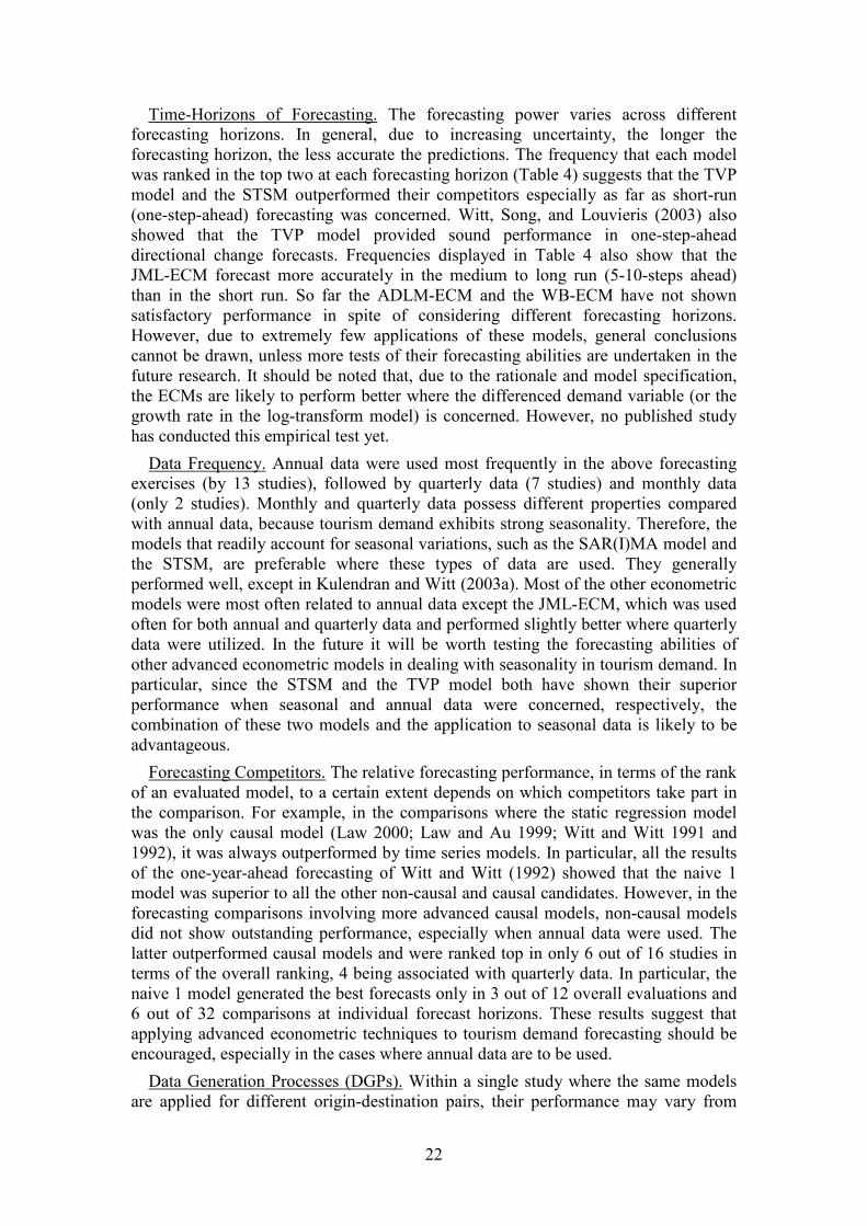
Time-Horizons of Forecasting. The forecasting power varies across different

forecasting horizons. In general, due to increasing uncertainty, the longer the

forecasting horizon, the less accurate the predictions. The frequency that each model

was ranked in the top two at each forecasting horizon (Table 4) suggests that the TVP

model and the STSM outperformed their competitors especially as far as short-run

(one-step-ahead) forecasting was concerned. Witt, Song, and Louvieris (2003) also

showed that the TVP model provided sound performance in one-step-ahead

directional change forecasts. Frequencies displayed in Table 4 also show that the

JML-ECM forecast more accurately in the medium to long run (5-10-steps ahead)

than in the short run. So far the ADLM-ECM and the WB-ECM have not shown

satisfactory performance in spite of considering different forecasting horizons.

However, due to extremely few applications of these models, general conclusions

cannot be drawn, unless more tests of their forecasting abilities are undertaken in the

future research. It should be noted that, due to the rationale and model specification,

the ECMs are likely to perform better where the differenced demand variable (or the

growth rate in the log-transform model) is concerned. However, no published study

has conducted this empirical test yet.

Data Frequency. Annual data were used most frequently in the above forecasting

exercises (by 13 studies), followed by quarterly data (7 studies) and monthly data

(only 2 studies). Monthly and quarterly data possess different properties compared

with annual data, because tourism demand exhibits strong seasonality. Therefore, the

models that readily account for seasonal variations, such as the SAR(I)MA model and

the STSM, are preferable where these types of data are used. They generally

performed well, except in Kulendran and Witt (2003a). Most of the other econometric

models were most often related to annual data except the JML-ECM, which was used

often for both annual and quarterly data and performed slightly better where quarterly

data were utilized. In the future it will be worth testing the forecasting abilities of

other advanced econometric models in dealing with seasonality in tourism demand. In

particular, since the STSM and the TVP model both have shown their superior

performance when seasonal and annual data were concerned, respectively, the

combination of these two models and the application to seasonal data is likely to be

advantageous.

Forecasting Competitors. The relative forecasting performance, in terms of the rank

of an evaluated model, to a certain extent depends on which competitors take part in

the comparison. For example, in the comparisons where the static regression model

was the only causal model (Law 2000; Law and Au 1999; Witt and Witt 1991 and

1992), it was always outperformed by time series models. In particular, all the results

of the one-year-ahead forecasting of Witt and Witt (1992) showed that the naive 1

model was superior to all the other non-causal and causal candidates. However, in the

forecasting comparisons involving more advanced causal models, non-causal models

did not show outstanding performance, especially when annual data were used. The

latter outperformed causal models and were ranked top in only 6 out of 16 studies in

terms of the overall ranking, 4 being associated with quarterly data. In particular, the

naive 1 model generated the best forecasts only in 3 out of 12 overall evaluations and

6 out of 32 comparisons at individual forecast horizons. These results suggest that

applying advanced econometric techniques to tourism demand forecasting should be

encouraged, especially in the cases where annual data are to be used.

Data Generation Processes (DGPs). Within a single study where the same models

are applied for different origin-destination pairs, their performance may vary from

23

case to case. An extreme example can be seen in the results of Li, Song, and Witt

(2002), where the ARIMA model was shown to generate the most accurate forecasts

in the cases of Japan and Singapore, while the second poorest for Australia and the

US. Furthermore, the WB-ECM outperforms all the other candidates in Australia’s

case, but is ranked the last second in the UK’s case. Similar phenomena can also be

seen in Kim and Song (1998), Kulendran and King (1997), Kulendran and Wilson

(2000) and so on. Such discrepancies in models’ performance across different

countries may well result from different DGPs relating to these destinations or origins,

especially in the cases where destination- or origin-specific one-off events take place.

A model’s ability to capture the intervention effect on the time series may also

affect predictive accuracy. Within the tourism context, however, the impact of

interventions, as well as outlier detection, has only been assessed for timeseries

models (see, for instance, Goh and Law 2002; Chu 2004). No study has examined the

effects of interventions or outliers on the forecasting performance of econometric

models.

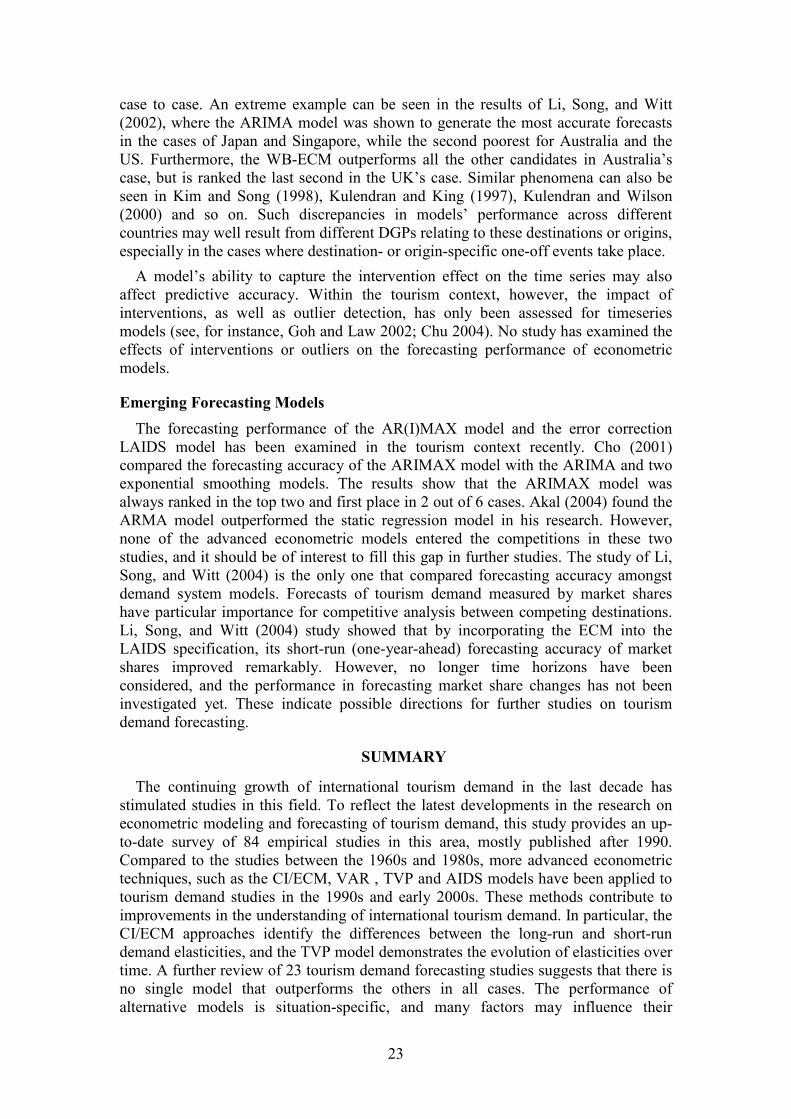
Emerging Forecasting Models

The forecasting performance of the AR(I)MAX model and the error correction

LAIDS model has been examined in the tourism context recently. Cho (2001)

compared the forecasting accuracy of the ARIMAX model with the ARIMA and two

exponential smoothing models. The results show that the ARIMAX model was

always ranked in the top two and first place in 2 out of 6 cases. Akal (2004) found the

ARMA model outperformed the static regression model in his research. However,

none of the advanced econometric models entered the competitions in these two

studies, and it should be of interest to fill this gap in further studies. The study of Li,

Song, and Witt (2004) is the only one that compared forecasting accuracy amongst

demand system models. Forecasts of tourism demand measured by market shares

have particular importance for competitive analysis between competing destinations.

Li, Song, and Witt (2004) study showed that by incorporating the ECM into the

LAIDS specification, its short-run (one-year-ahead) forecasting accuracy of market

shares improved remarkably. However, no longer time horizons have been

considered, and the performance in forecasting market share changes has not been

investigated yet. These indicate possible directions for further studies on tourism

demand forecasting.

SUMMARY

The continuing growth of international tourism demand in the last decade has

stimulated studies in this field. To reflect the latest developments in the research on

econometric modeling and forecasting of tourism demand, this study provides an up-

to-date survey of 84 empirical studies in this area, mostly published after 1990.

Compared to the studies between the 1960s and 1980s, more advanced econometric

techniques, such as the CI/ECM, VAR , TVP and AIDS models have been applied to

tourism demand studies in the 1990s and early 2000s. These methods contribute to

improvements in the understanding of international tourism demand. In particular, the

CI/ECM approaches identify the differences between the long-run and short-run

demand elasticities, and the TVP model demonstrates the evolution of elasticities over

time. A further review of 23 tourism demand forecasting studies suggests that there is

no single model that outperforms the others in all cases. The performance of

alternative models is situation-specific, and many factors may influence their

24

forecasting accuracy. In general, the TVP model and the STSM perform relatively

well, especially for short-run forecasting. Where advanced econometric models

compete with their univariate time-series counterparts or the conventional benchmark

no-change model, the econometric models tend to outperform the others, especially as

far as annual data are concerned.

Some emerging models have shown advantages in modeling and forecasting

international tourism demand. Broader applications and further improvements of these

methodologies are likely to benefit research in this area. In particular, the following

directions are of interest and value in future econometric studies of tourism demand.

1. Further application of the AIDS/LAIDS especially its ECM form for analyzing

and predicting market shares and their variations.

2. Combination of the STSM and TVP model to forecast seasonal tourism

demand.

3. Further employment of the AR(I)MAX model and examination of its

forecasting performance in comparison with other econometric models.

4. Comparison of the abilities of alternative models to forecast tourism demand

changes (or growth).

5. Investigation of the forecasting performance of advanced econometric models

in dealing with seasonality in tourism demand.

In view of the diversity of research findings, including those derived from newly

emerging techniques which has resulted in a relatively small number of observations

in this survey (especially those related to forecasting comparison), caution should be

exercised in interpreting the generalized findings of this paper.

REFERENCES

Akal, M. (2004). “Forecasting Turkey's Tourism Revenues by ARMAX Model.” Tourism

Management, 25: 565-80.

Akis, S. (1998). “A Compact Econometric Model of Tourism Demand for Turkey.” Tourism


Ashworth, J. and P. Johnson (1990). “Holiday Tourism Expenditure: Some Preliminary

Econometric Results.” The Tourist Review, 3: 12-19.

Bakkal, I. (1991). “Characteristics of West German Demand for International Tourism in the

Northern Mediterranean Region.” Applied Economics, 23:295-304.

Cho, V. (2001). “Tourism Forecasting and Its Relationship with Leading Economic

Indicators.” Journal of Hospitality and Tourism Research, 25(4): 399-420.

Chu, F. (2004). “Forecasting Tourism Demand: A Cubic Polynomial Approach.” Tourism


Crouch, G. I. (1992). “Effect of Income and Price on International Tourism.” Annals of

Tourism Research, 19: 643-64.

——(1994a). “Demand Elasticities for Short-Haul versus Long-Haul Tourism.” Journal of

Travel Research, 33: 2-7.

——(1994b). “The Study of International Tourism Demand: A Review of Findings.” Journal

of Travel Research, 33: 12-23.

25

——(1994c). “The Study of International Tourism Demand: A Survey of Practice.” Journal of


——(1995). “A Meta-Analysis of Tourism Demand.” Annals of Tourism Research, 22: 103-

18.

——(1996). “Demand Elasticities in International Marketing: A Meta-Analytical Application

to Tourism.” Journal of Business Research, 36: 117-36.

De Mello, M., A. Pack and M. T. Sinclair (2002). “A System of Equations Model of UK

Tourism Demand in Neighbouring Countries.” Applied Economics, 34: 509-521.

Deaton, A. S. and J. Muellbauer (1980). “An Almost Ideal Demand System.” American

Economic Review, 70: 312-26.

Di Matteo, L. (1999). “Using Alternative Methods to Estimate the Determinants of Cross-

Border Trips.” Applied Economics, 31: 77-88.

Di Matteo, L. and R. Di Matteo (1993). “The Determinants of Expenditures by Canadian

Visitors to the United States.” Journal of Travel Research, 31: 34-42.

Divisekera, S. (2003). “A Model of Demand for International Tourism.” Annals of Tourism

Research, 30: 31-49.

Dritsakis, N. (2004). “Cointegration Analysis of German and British Tourism Demand for

Greece.” Tourism Management, 25: 111-19.

Dritsakis, N. and J. Papanastasiou (1998). “An Econometric Investigation of Greek Tourism:

A Note.” Journal for Studies in Economics and Econometrics, 22: 115-22.

Dritsakis, N. and S. Athanasiadis (2000). “An Econometric Model of Tourist Demand: The

Case of Greece.” Journal of Hospitality and Leisure Marketing, 7: 39-49.

Durbarry, R. and M. T. Sinclair (2003). “Market Shares Analysis: The Case of French

Tourism Demand.” Annals of Tourism Research, 30: 927-41.

Engle, R. F. and C. W. J. Granger (1987). “Cointegration and Error Correction:

Representation, Estimation and Testing.” Econometrica, 55: 251-76.

Friedman, M. (1956). A Theory of the Consumption Function. Princeton University Press.

Fujii, E., M. Khaled and J. Mark (1985). “An Almost Ideal Demand System for Visitor

Expenditures.” Journal of Transport Economics and Policy, 19: 161-71.

Gallet, C. A. and B. M. Braun (2001). “Gradual Switching Regression Estimates of Tourism

Demand.” Annals of Tourism Research, 28: 503-08.

García-Ferrer, A. and R. Queralt (1997). “A Note on Forecasting International Tourism

Demand in Spain.” International Journal of Forecasting, 13: 539-49.

Gerakis, A. S. (1965). “Effects of Exchange-Rate Devaluations and Revaluations on Receipts

from Tourism.” International Monetary Fund Staff Papers, 12: 365-84.

Goh, C. and R. Law (2002). “Modeling and Forecasting Tourism Demand for Arrivals with

Stochastic Nonstationary Seasonality and Intervention.” Tourism Management, 23: 499-

510.

González, P. and P. Moral (1995). “An Analysis of the International Tourism Demand in

Spain.” International Journal of Forecasting, 11: 233-51.

——(1996). “Analysis of Tourism Trends in Spain.” Annals of Tourism Research, 23: 739-

54.

Gray, H. P. (1966). “The Demand for International Travel by United States and Canada.”

International Economic Review, 7: 83-92.

Greenidge, K. (2001). “Forecasting Tourism Demand: An STM Approach.” Annals of

Tourism Research, 28: 98-112.

26

Guthrie, H. W. (1961). “Demand for Tourists’ Goods and Services in a World Market.”

Papers and Proceedings of the Regional Science Association, 7: 159-75.

Harris, R. and R. Sollis (2003). Applied Tme Series Modeling and Forecasting. Wiley:

Chichester.

Hendry, D. F. (1995). Dynamics Economics: Advanced Text in Econometrics. Oxford

University Press: Oxford.

Holmes, R. A. and, A. F. M. Shamsuddin (1997). “Short- and Long-Term Effects of World

Exposition 1986 on US Demand for British Columbia Tourism.” Tourism Economics, 3:

137-60.

Icoz, O., T. Var, and, M. Kozaka (1998). “Tourism Demand in Turkey.” Annals of Tourism

Research, 25: 236-40.

Ismail, J. A., T. J. Iverson and, L. A. Cai (2000). “Forecasting Japanese Arrivals to Guam: An

Empirical Model.” Journal of Hospitality and Leisure Marketing,7: 51-63.

Jensen, T. C. (1998). “Income and Price Elasticities by Nationality for Tourists in Denmark.”

Tourism Economics, 4: 101-30.

Johansen, S. (1988). “A Statistical Analysis of Cointegration Vectors.” Journal of Economic

Dynamics and Control, 12: 231-54.

Jørgensen, F. and, G. Solvoll (1996). “Demand Models for Inclusive Tour Charter: The

Norwegian Case.” Tourism Management, 17: 17-24.

Kim, S. and H. Song (1998). “Analysis of Tourism Demand in South Korea: A Cointegration

and Error Correction Approach.” Tourism Analysis, 3: 25-41.

Kim, Y. and, M. Uysal (1998). “Time-Dependent Analysis for International Hotel Demand in

Seoul.” Tourism Economics, 4: 253-63.

Kulendran, N. (1996). “Modelling Quarterly Tourism Flows to Australia.” Tourism

Economics, 2: 203-22.

Kulendran, N. and K. Wilson (2000). “Modelling Business Travel.” Tourism Economics, 6:

47-59.

Kulendran, N. and M. King (1997). “Forecasting International Quarterly Tourism Flows

Using Error Correction and Time Series Models.” International Journal of Forecasting,

13: 319-27.

Kulendran, N. and S. F. Witt (2001). “Cointegration versus Least Squares Regression.”

Annals of Tourism Research, 28: 291-311.

——(2003a). “Forecasting the Demand for International Business Tourism.” Journal of


——(2003b). “Leading Indicator Tourism Forecasts.” Tourism Management, 24: 503-10.

Lanza, A. P. Temple and G. Urga (2003). “The Implications of Tourism Specialisation in the

Long Run: An Econometric Analysis for 13 OECD Economies.” Tourism Management,

24: 315-21.

Lathiras, P. and, C. Siriopoulos (1998). “The Demand for Tourism to Greece: A Cointegration

Approach.” Tourism Economics, 4: 171-85.

Law, R. (2000). “Back-propagation Learning in Improving the Accuracy of Neural Network-

based Tourism Demand Forecasting.” Tourism Management, 21: 331-40.

Law, R. and N. Au (1999). “A Neural Network Model to Forecast Japanese Demand for

Travel to Hong Kong.” Tourism Management, 20: 89-97.

Ledesma-Rodríguez, F. J., M. Navarro-Ibánez and J. V. Pérez-Rodríguez (2001). “Panel Data

and Tourism: A Case Study of Tenerife.” Tourism Economics, 7: 75-88.

Lee, C. K., T. Var and T. W. Blaine (1996). “Determinants of Inbound Tourism Expenditure.”


27

Li, G., H. Song and S. F. Witt (2002). “Econometric Analysis and Forecasts of International

Tourism Demand in Thailand.” Paper presented at the Fifth Biennial Conference on

Tourism in Asia: Development, Marketing and Sustainability, Hong Kong, May 23-25,

2002.

——(2004). “Modelling Tourism Demand: A Dynamic Linear AIDS Approach.” Journal of


Lim, C. (1997a). “An Econometric Classification and Review of International Tourism

Demand Models.” Tourism Economics, 3: 69-81.

——(1997b). “Review of International Tourism Demand Models.” Annals of Tourism

Research, 24: 835-49.

——(1999). “A Meta-Analytic Review of International Tourism Demand.” Journal of Travel

Research, 37: 273-84.

Lim, C. and M. McAleer (2001). “Cointegration Analysis of Quarterly Tourism Demand by

Hong Kong and Singapore for Australia.” Applied Economics, 33: 1599-619.

——(2002). “Time Series Forecasts of International Travel Demand for Australia.” Tourism


Lyssiotou, P. (2001). “Dynamic Analysis of British Demand for Tourism Abroad.” Empirical


Mangion, M. L., R. Durbarry and M. T. Sinclair (2003). “AIDS and Hedonic Pricing Models:

Their Relevance to Tourism Practitioners.” Paper presented at the Tourism Modelling

and Competitiveness Conference, Paphos, Cyprus.

Morley, C. L. (1997). “An Evaluation of the Use of Ordinary Least Squares for Estimating

Tourism Demand Model.” Journal of Travel Research, 35: 69-73.

——(1998). “A Dynamic International Demand Model.” Annals of Tourism Research, 25:

70-84.

Morris, A., K. Wilson and, S. Bakalis (1995). “Modelling Tourism Flows from Europe to

Australia.” Tourism Economics, 1: 147-67.

O’Hagan, J. W. and M. J. Harrison (1984). “Market Shares of US Tourism Expenditure in

Europe: An Econometric Analysis.” Applied Economics, 16: 919-31.

Papatheodorou, A. (1999). “The Demand for International Tourism in the Mediterranean

Region.” Applied Economics, 31: 619-30.

Payne, J. E. and A. Mervar (2002). “A Note on Modelling Tourism Revenues in Croatia.”

Tourism Economics, 8:103-09.

Pesaran, M. H. and Y. Shin (1995). “An Autoregressive Distributed Lag Modelling Approach

to Cointegration Analysis.” In Strom, S., A. Holly and P. Diamond, eds., Centennial Vol.

of Rangar Frisch, Econometric Society Monograph. Cambridge University Press:

Cambridge.

Pyo, S., M. Uysal and R. McLellan (1991). “A Linear Expenditure Model for Tourism

Demand.” Annals of Tourism Research, 31: 619-30.

Qiu, H. and J. Zhang (1995). “Determinants of Tourist Arrivals and Expenditures in Canada.”

Journal of Travel Research, 34: 43-49.

Qu, H. and, S. Lam (1997). “A Travel Demand Model for Mainland Chinese Tourists to Hong

Kong.” Tourism Management, 18: 593-97.

Riddington, G. (1999). “Forecasting Ski Demand: Comparing Learning Curve and Time

Varying Parameter Approaches.” Journal of Forecasting, 18: 205-14.

Rossello-Nadal, J. (2001). “Forecasting Turning Points in International Visitor Arrivals in the

Balearic Islands.” Tourism Economics, 7: 365-80.

28

Rosselló-Nadal, J., A. Riera-Font and A. Sansó-Rosselló (2004). “The Economic

Determinants of Seasonal Patterns.” Annals of Tourism Research, 31: 697-711.

Shan, J. and, K. Wilson (2001). “Causality between Trade and Tourism: Empirical Evidence

from China.” Applied Economics Letters, 8: 279-83.

Sheldon, P. J. (1993). “Forecasting Tourism: Expenditure versus Arrivals.” Journal of Travel

Research, 32: 13-20.

Sheldon, P. J. and T. Var (1985). “Tourism Forecasting: A Review of Empirical Research.”

Journal of Forecasting, 4: 183-95.

Smeral, E. and S. Witt (1996). “Econometric Forecasts of Tourism Demand to 2005.” Annals

of Tourism Research, 23: 891-907.

Smeral, E. and, A. Weber (2000). “Forecasting International Tourism Trends to 2010.”


Smeral, E., S. F. Witt and C. A. Witt (1992). “Econometric Forecasts: Tourism Trends to

2000.” Annals of Tourism Research, 29: 450-66.

Song, H. and K. F. Wong (2003). “Tourism Demand Modeling: A Time-Varying Parameter

Approach.” Journal of Travel Research, 42: 57-64.

Song, H., K. F. Wong and K. S. Chon (2003). “Modelling and Forecasting the Demand for

Hong Kong Tourism.” International Journal of Hospitality Management, 22: 435-51.

Song, H., P. Romilly and X. Liu (2000). “An Empirical Study of Outbound Tourism Demand

in the U.K..” Applied Economics, 32: 611-24.

Song, H., S. F. Witt and G. Li (2003). “Modelling and Forecasting the Demand for Thai

Tourism.” Tourism Economics, 9: 363-87.

Song, H., S. F. Witt and T. C. Jensen (2003). “Tourism Forecasting: Accuracy of Alternative

Econometric Models.” International Journal of Forecasting, 19: 123-41.

Stone, J. R. N. (1954). “Linear Expenditure Systems and Demand Analysis: An Application

to the Pattern of British Demand.” Economic Journal, 64: 511-27.

Syriopoulos, T. (1995). “A Dynamic Model of Demand for Mediterranean Tourism.”

International Review of Applied Economics, 9: 318-36.

Syripopoulos, T. and T. Sinclair (1993). “A Dynamic Model of Demand for Mediterranean

Countries.” Applied Economics, 25: 1541-52.

Theil, H. (1966). Applied Economic Forecasting. North-Holland: Amsterdam.

Turner, L. W. and S. F. Witt (2001a) “Factors Influencing Demand for International Tourism:

Tourism Demand Analysis Using Structural Equation Modelling, Revisited.” Tourism


——(2001b). “Forecasting Tourism Using Univariate and Multivariate Structural Time Series

Models.” Tourism Economics, 7: 135-47.

Turner, L. W., Y. Reisinger and S. F. Witt (1998). “Tourism Demand Analysis Using

Structural Equation Modelling.” Tourism Economics, 4: 301-23.

Uysal, M. and J. L. Crompton (1985). “An Overview of Approaches Used to Forecast

Tourism Demand.” Journal of Travel Research, 24: 7-15.

Uysal, M. and M. Roubi (1999). “Artificial Neural Networks versus Multiple Regression in

Tourism Demand Analysis.” Journal of Travel Research, 38: 111-18.

Vanegas, M., Sr and R. R. Croes (2000). “Evaluation of Demand: US Tourists to Aruba.”


Var, T. and G. M. Icoz (1990). “Factors Affecting International Tourism Demand for

Turkey.” Annals of Tourism Research, 17: 606-10.

29

Vogt, M. G. and C. Wittayakorn (1998). “Determinants of the Demand for Thailand’s Exports

of Tourism.” Applied Economics, 30: 711-15.

White, K. J. (1985). “An International Travel Demand Model: US Travel to Western Europe.”


Wickens, M. R. and T. S. Breusch (1988). “Dynamic Specification, the Long-Run and the

Estimation of Transformed Regression Model.” Economic Journal, 98 (Conference):

189-205.

Witt, C. A. and S. F. Witt (1990) “Appraising an Econometric Forecasting Model.” Journal of


Witt, S. F. and C. A. Witt (1991) “Tourism Forecasting: Error Magnitude, Direction of

Change Error and Trend Change Error.” Journal of Travel Research, 30: 26-33.

——(1992). Modeling and Forecasting Demand in Tourism. Academic Press: London.

——(1995). “Forecasting Tourism Demand: A Review of Empirical Research.” International

Journal of Forecasting, 11: 447-75.

Witt, S.F., H. Song and P. Louvieris (2003). “Statistical Testing in Forecasting Model

Selection.” Journal of Travel Research, 42: 151-58.

Zellner, A. C. (1962). “An Efficient Method of Estimating Seemingly Unrelated Regressions

and Test for Aggregation Bias.” Journal of the American Statistical Association, 57:

348-68

Documents

Recent Developments in Econometric Modeling and …epubs.surrey.ac.uk/7525/2/recent developments.pdfRecent Developments in Econometric Modeling and Forecasting GANG LI a, HAIYAN SONG