Embed Size (px)
Citation preview
Cav03-OS-6-012 Fifth International Symposium on Cavitation (CAV2003)
Osaka, Japan, November 1-4, 2003
Prediction of Cavitation Performance of Axial Flow Pump by Using Numerical Cavitating Flow Simulation with Bubble Flow Model
ABSTRACTThe prediction of cavitation performance by using a
numerical flow simulation is significant to reduce the productivecost when designing a pump impeller blade. The cavitation hasseveral appearances in the pump such as sheet cavitation, cloudcavitation, and vortex cavitation. Cloud cavitation is composedof a lot of tiny bubbles with complex behavior. The bubble flowmodel is a cavitation model for numerical simulation, in whichthe bubble dynamics is treated in detail.
In this study, we develop a new numerical simulation codethat includes the bubble flow model. The code considers thedistribution of the number density of bubbles, and thetransitional and volumetric motions of bubbles. It was applied toa rotating flow in an axial flow pump. The predicted cavitationperformance of the pump agreed qualitatively with theexperiment. The predicted cavitation distribution on the impellerblade also agreed with that visualized. The code has the potentialto simulate bubble behavior in cavitation erosion.
INTRODUCTIONWhen a pump is downsized from the viewpoint of cost
reduction, the relative flow velocity increases near the impellerblades. As a result, the reduction of cavitation performance andthe cavitation erosion become significant problems. Recently,numerical cavitating flow simulations have been applied torotating machinery such as pumps, inducers, and water turbines[1-7]. The reports on these simulations predict the cavitatingflow pattern and the cavitation performance. However, cavitationerosion has not been focused on yet. Cavitation erosionespecially occurs when cloud and vortex cavitations appear inthe turbomachinery. Cavitation erosion has a close relation withbubble behavior, therefore, bubble dynamics needs to bepredicted to simulate cavitation erosion.
The bubble flow model [7,8] is a representative model forthe numerical cavitating flow simulation. In this model, a lot oftiny spherical bubbles are initially assumed to be in the flow. Thebubble volume varies with the pressure difference between thebubbles and the liquid. The variations in the bubble radius andbubble pressure are described with the Rayleigh-Plesset equation.A void fraction is obtained from the bubble radius and thenumber density of the bubbles.
In the previous study [9], we applied a numerical cavitatingflow simulation including the bubble flow model to six axialflow pumps with different blade profiles, blade angles, andnumber of blades. To reduce the calculation time, a two-dimensional isolated hydrofoil simulation was conducted tocalculate the lift and drag coefficients. The total head of thepump was calculated from the cavitation performance of the fivehydrofoils that constitute the impeller blade. The predictedvariation of the total head against NPSH qualitatively agreedwith the experimental data.
In the present study, we developed a bubble-flow-modelsimulation code for the turbomachinery and applied it to an axialflow pump. We then evaluated the cavitation performance of thepump, the distributions of the liquid pressure and the voidfraction, and also the distributions of the number density of thebubbles, the bubble radius and the bubble pressure. The resultssuggest that this code can possibly to simulate bubble behaviorin cavitation erosion. NOMENCLATURE
c: coefficient for pseudocompressibilityC: chord lengthd: diameter of cylindrical surfaceD: diameter of blade tip
Masashi FukayaMechanical Engineering Research Laboratory
Hitachi, Ltd.502, Kandatsu, Tsuchiura, Ibaraki 300-0013, JAPAN
Tomoyoshi OkamuraResearch & Development Laboratory
Hitachi Industries Co.,Ltd.603, Kandatsu, Tsuchiura, Ibaraki 300-0013, JAPAN
Yoichiro MatsumotoDepartment of Mechanical Engineering
University of Tokyo7-3-1, Hongo, Bunkyo-ku, Tokyo 113-8656, JAPAN
Yoshiaki TamuraDepartment of Computational Science and Engineering
Toyo University2100, Kujirai, Kawagoe, Saitama 350-8585, JAPAN
1
f: volume fraction: fluxes in �, �, ��direction
H: head
H : source term
g: acceleration due to gravityL: cavitation length
NPSH: Net Positive Suction HeadQ: flow rate
Q: unknown vector
p: pressurer: bubble radius
Re: Reynolds numbert: time
T: surface tensionu, v, w: velocity
U, V, W contravariant velocityUt: peripheral velocity at blade tip�: head coefficient�: viscosity�: rotating speed�: density
Subscriptscal: calculatedexp: experimental
B: bubbled: design pointG: gas phasei: x, y and z directionsj: ξ,η and ζ directions
L: liquid phaseR: three-percent drop of total head v: vapor
NUMERICAL METHODGoverning Equations
The following assumptions concerning the bubbles in theflow are made in the simulation code.・ The gas phase consisting of spherical bubbles is compressible.・ No collision and coalescence occurs. The bubbles are filled
with vapor and non-condensable gas.・ The effects of evaporation and condensation on the bubble
surface are modeled according to the pressure variation of thenon-condensable gas. Non-condensable gas pressure varieswith isothermal expansion and adiabatic contraction [10].Mass transfer between the gas and the liquid phases isnegligibly small compared to liquid mass.
・ The density and momentum of the gas phase are small enoughto be negligible.
The governing equations are summarized as follows,
, ,
, ,
where F , G , vF and vG are not described. Equation (1) iscomposed ofa) the conservation of the volumetric fraction of the liquid phase,
b) the conservation of momentum,c) a pressure equation based on pseudo-compressibility, which
is derived form the conservation of the volumetric fractionsd) and the conservation of the number density of bubbles.
In Eq. (1), the liquid and gas velocities mean the absolutevelocities in a rotating coordinate system. Therefore, Coriolis’force appears in the source term H .
The volumetric motion of a bubble is described by theRayleigh-Plesset equation [11],
where both T and pv are constant. To avoid divergence in thecalculation, the viscorsity � in Eq. (3) is assumed to be muchlarger than that of the actual flow.
Cavitation is expressed as the increase of the void fraction,which is calculated by the following equation,
The translational motion of a bubble is solved consideringthe force balance of the bubble,
where FAi is the added mass force,
is a constant of 0.5 for a spherical bubble, Fpi is the force ofthe acceleration of the surrounding fluid,
GFE ˆ,ˆ,ˆ
, (2)
DtDr
rrTppp G
GGvGB
142����� , (3)
HGFEGFEtQ vvv ˆˆˆˆˆˆˆˆ
��
��
�
��
�
��
�
��
�
��
�
��
�
�
������, (1)
J
np
wfvfuf
f
Q
G
LLL
LLL
LLL
L
/ˆ
��������
�
�
��������
�
�
��
�
�
J
UnUfcUfc
pUwf
pUvfpUuf
Uf
E
GG
GGLLLL
zLLLL
yLLLL
xLLLL
LL
/ˆ
22
��������
�
�
��������
�
�
�
�
�
�
�
��
��
��
��
JEzzzzyyzxx
yzzyyyyxx
xzzxyyxxx
v /
00
0
ˆ
��������
�
�
��������
�
�
��
��
��
�������
������
������
�
GGG nrf 3
34�� . (4)
, (5)
, (6)
2
J
tDrD
nrc
uv
H
G
GGGGL
LL
LL
/
0
4
0
0
ˆ
22
���������
�
�
���������
�
�
��
�
��
�
�
))((41)(
23 2
2
2
GiLiGiLiL
LBGGG uuuu
ppDt
DrDt
rDr ���
�
��
�
� � � ���
���
��
���
��
��
�
�
��
�
��
j
GiGLGj
GiGLAi
urU
tur
F�
����
33
34
� � � ���
���
��
���
��
��
�
�
��
�
��
j
LiGLLj
LiGL urU
tur
�
��33
0����� CiLiDipiAi FFFFF
FDi and FLi are the drag and lift forces,
where L�
�
is the vorticity vector, and FCi is the Coriolis’ force,
Based on Eqs. (5)-(13), the relative velocity of the bubbleto the liquid phase is solved with the bubble radius, the liquidvelocity and so on. The details of the governing equations andthe algorithm of the calculation are described in Ref. [7].
The Reynolds number of the flow in this simulation is8.5�105. However, no turbulent model is used in the simulationcode. The introduction of the turbulent model into the code is asubject for study in the near future.
Simulated Region and Boundary ConditionsThe developed simulation code is applied to an axial flow
pump that operates at a high specific speed. The fluid is water ata temperature of 293 K. The pump has four impeller blades. Theblade profile is based on the NACA 65 series. The flow rate ofwater at the design point is 24.1 m3/min. The blade-tip diameteris 280 mm and the hub diameter is 102 mm.
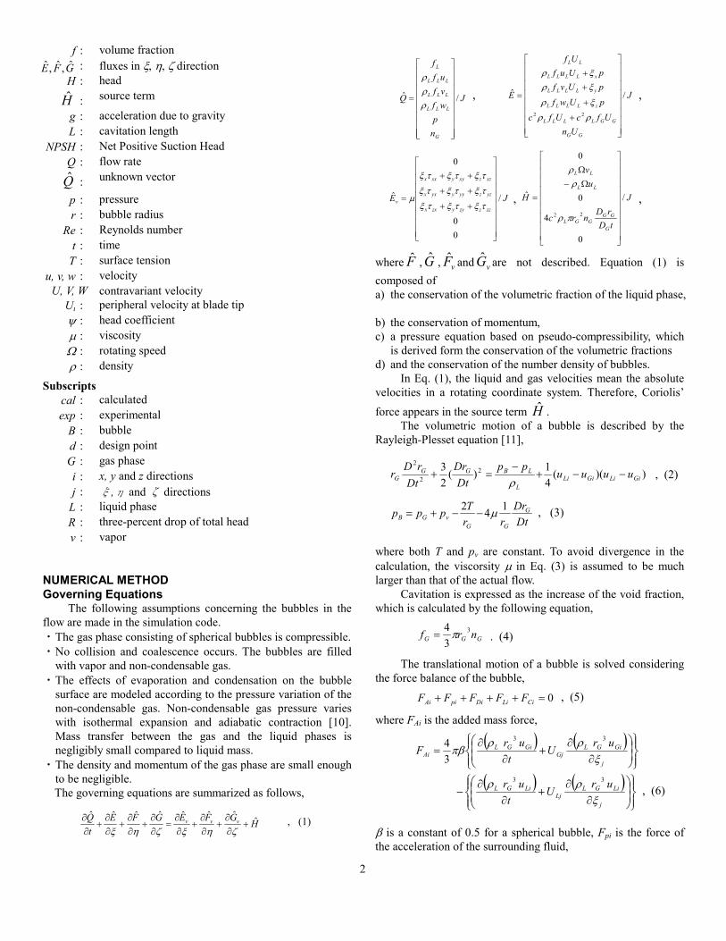
Figure 1 shows the numerical mesh and the boundaryconditions in the simulation. A region between the pressure sideand suction sides of the impeller blades is investigated by usingperiodical boundaries. Cylindrical upstream and downstreamchannels of 0.5 m are connected to the region that includes theimpeller blades. The tip clearance between the impeller bladeand the casing is not considered in this simulation. The gridnumbers are 75, 29 and 29 in the axial, radial and peripheraldirections. At the inlet boundary, the following is assumed. ・ To fix the flow rate, the liquid velocity is uniform constant at
be 7.29 m/s. There is no velocity difference between the liquidphase and the bubbles.
・ The void fraction of 0.001 and the bubble radius of 1.0�10-5
m are given. The number density of the bubbles becomes2.39�1011 m-3.
・ The o
change the NPSH condition. Other parameters such as the liquidand bubble velocities, the bubble radius, and the number densityof the bubbles have the Neumann condition at the outlet. Non-slip condition is assumed on the casing wall, and the peripheralvelocity caused by the impeller rotation is added on the surfacesof impeller blade and hub. For other parameters except the liquidand bubble velocities, the Neumann condition is assumed on thecasing wall and the surfaces of impeller blade and hub.
RESULTS AND DISCUSSIONCavitation Performance
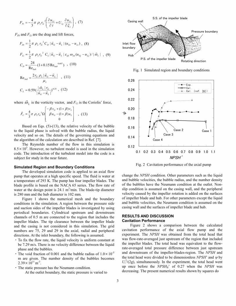
Figure 2 shows a comparison between the calculatedcavitation performance of the axial flow pump and theexperiment. The NPSH was obtained from the total head thatwas flow-rate-averaged just upstream of the region that includedthe impeller blades. The total head was equivalent to the flow-rate-averaged total pressure difference between just upstreamand downstream of the impeller-blades-region. The NPSH andthe total head were divided to be dimensionless NPSH’ and � byUt
2/(2g), simultaneously. In the experiment, the total head wentup once before the NPSHR’ of 0.27 when the NPSH wasd s do
0.12
0.14
0.16
0.18
0.20
0.22
0.24
0.26
0.1 0.2 0.3 0.4 0.5 0.6 0.7 0.8 0.9 1.0 1.1
NPSH’
ψ
0.12
0.14
0.16
0.18
0.2
0.22
0.24
0.26
0.1 0.2 0.3 0.4 0.5 0.6 0.7 0.8 0.9 1 1.1
Exp.Cal.Cal. (ref. [?])
Case 1Case 2
Case 3
Case 4
[9]
||/)(||21 2
LLjGjLkijkLGLGLLi uuuuCrF ��������
���
��
�
�
��
�
�
�
��
�
�
j
LiLj
LiGLPi
uU
tu
rF�
��3
34 , (7)
)(||21 2
LiGiLGDGLDi uuuuCrF ���
��
��
)Re15.01(Re
24 687.0bub
bubDC ��
L
LGLGbub
uur�
� ||2Re
��
�
�
25.0)||
||(59.0
LG
GLL uu
rC
��
�
�
�
�
, (8)
, (9)
, (10)
, (11)
, (12)
Fig. 1 Simulated region and boundary conditions
P.S. of the impeller blade
S.S. of the impeller blade
Pressure boundary
Inlet flowboundary
Rotating direction
Casing wall
Hub
Fig. 2 Cavitation performance of the axial pump
���
�
�
���
�
�
��
���
0)1()1(
34 3
LG
LG
GLC uuvv
rF ��
��
���
, (13)
static pressure has the Neumann condition.At the outlet boundary, the static pressure is varied t
3
ecreasing. The present numerical results shown by square
Leading edge
Tip
Rotatingdirection
Cavitation
HubFlowdirection
(Edge of cavitation)
Flowdirection
Rotatingdirection
(b) Predicted(a) Observed
0.0
0.1
0.2
0.3
0.4
0.5
0.6
0.7
0.8
0.9
1.0
0.0 0.2 0.4 0.6 0.8 1.0 1.2
d/D
L/C
0
0.1
0.2
0.3
0.4
0.5
0.6
0.7
0.8
0.9
1
0 0.2 0.4 0.6 0.8 1 1.2
Cal.
Cal. (Ref. [?])
(Hub)
(Tip)
[9]
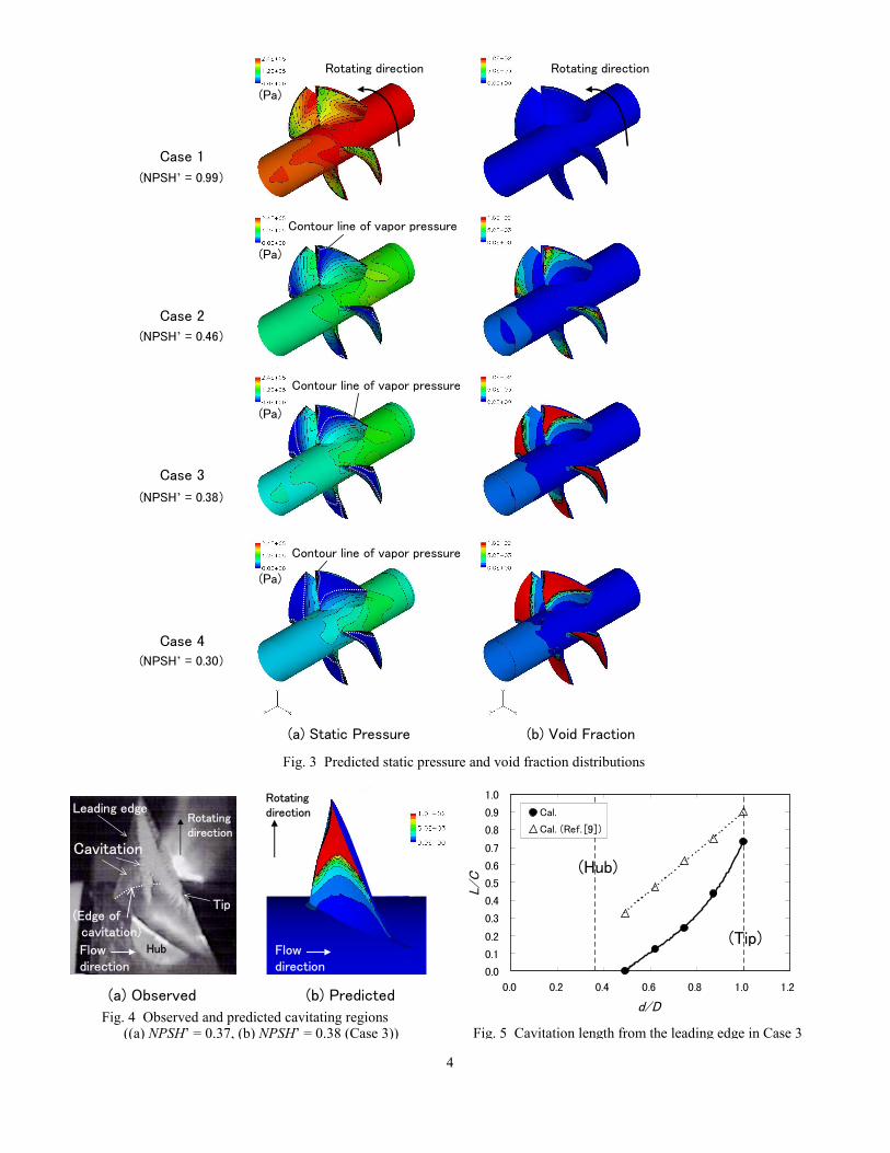
Fig. 4 Observed and predicted cavitating regions ((a) NPSH’ = 0.37, (b) NPSH’ = 0.38 (Case 3)) Fig. 5 Cavitation length from the leading edge in Case 3
Fig. 3 Predicted static pressure and void fraction distributions
(a) Static Pressure (b) Void Fraction
Case 1
Case 2
Case 3
Case 4
Contour line of vapor pressure
Contour line of vapor pressure
(Pa)
(Pa)
(Pa)
(Pa)
(NPSH’ = 0.99)
(NPSH’ = 0.46)
(NPSH’ = 0.38)
(NPSH’ = 0.30)
Rotating direction Rotating direction
Contour line of vapor pressure
4
not obviously have the local increase of the total head. Thepredicted cavitation performance of the pump, however, agreesqualitatively with the experiment. The predicted NPSHR’ was0.30.
Figure 2 also shows the previous numerical result [9] astriangles. In the previous study, the total head was obtained fromtwo-dimensional calculations of five isolated hydrofoilsconstituting an impeller blade. When the NPSH was high andcavitation did not occur, the predicted total head exceeded theexperiment. This result is valid because the losses caused by theleakage flow at the tip clearance, the secondary flow between theimpeller blades, and the boundary layer near the casing wallwere not considered in the previous simulation.
In the present simulation, on the other hand, the abovesecondary flow and the boundary layer are considered, resultingin a total head reduction compared to the previous prediction.The present prediction of the total head was lower than theexperiment. This is because no turbulent model is used in thepresent code and the simulated flow near the wall was notsufficiently exact. Furthermore, a lack of the numerical meshnumber is also suspicious. In the present simulation, the effect ofpressure interaction between the impeller blades is included.Although the predicted cavitation performance is not necessarilyin good quantitative agreement with the experiment, the flowaround the impeller blades is simulated well.
Cavitating RegionFigure 3 shows the numerical results of the static pressure
and the void fraction distributions in Cases 1-4 in Fig. 2. In staticpressure distributions, we draw the contour lines of the vaporpressure of 2300 Pa. In void fraction distributions, the redregions indicate that the void fraction is higher than 0.1. In Cases2, 3 and 4, the region below the vapor pressure corresponds well
with the region where the void fraction exceeds 0.1. In this study,therefore, the region where the void fraction is over 0.1 isregarded as the cavitating region. The cavitating regionnoticeably expands near the blade tip with a decrease in theNPSH’.
The observed and predicted cavitating regions arecompared in Fig. 4. Figure 4(a) shows an image taken by a high-speed camera from a nearly radial direction through the acryliccasing of the pump. Near the surface of the impeller blade, thecavitating region expands from the hub side to the blade-tip side,while the tip cavitation partially obstructs the view.
Figure 4(b) shows the void fraction distribution and thecavitating region colored red. Concerning the cavitating regionnear the impeller-blade surface, the prediction is in goodqualitative agreement with the observation.
The predicted cavitation length is shown in Fig. 5. Thecavitation length is defined as the distance between the leadingedge of the impeller blade and the downstream edge of thecavitating region. The cavitation length is measured on fivecylindrical surfaces between the hub and the tip of the impellerblade. The cavitation length L is nondimensionalized by thechord length C of a hydrofoil that is cut out from the impellerblade at each cylindrical surface.
In Fig. 5, the cavitation lengths predicted in the previousstudy are also shown as triangles. The previous cavitation lengthincreases at a constant rate with an increase in the radial position.In the present study, the increasing rate of the cavitation lengthnear the blade tip is larger than that near the hub. The presentresult is in better agreement with the observation shown in Fig.4(a) than the previous one.
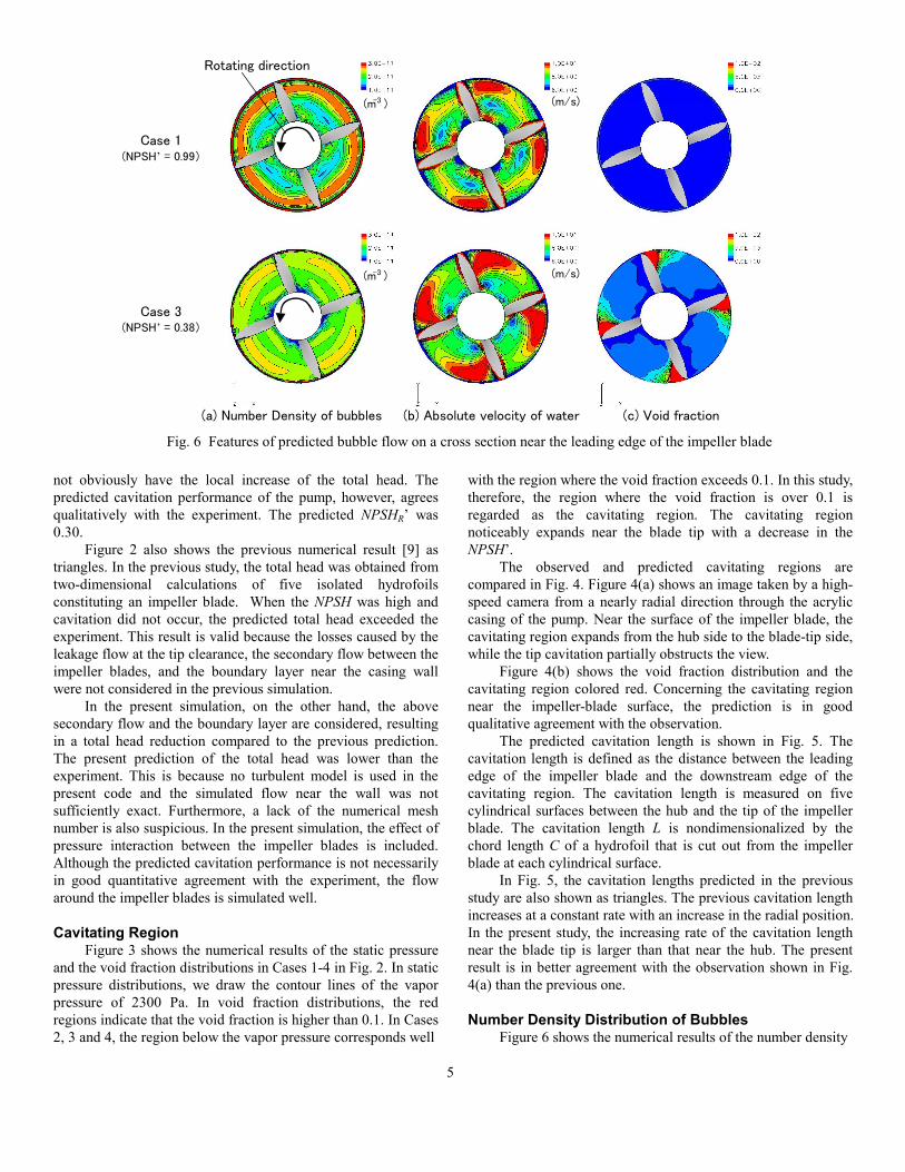
Number Density Distribution of BubblesFigure 6 shows the numerical results of the number density
(a) Number Density of bubbles
Case 1
Case 3
(NPSH’ = 0.99)
(NPSH’ = 0.38)
(b) Absolute velocity of water (c) Void fraction
Rotating direction
(m )-3 (m/s)
(m )-3 (m/s)
Fig. 6 Features of predicted bubble flow on a cross section near the leading edge of the impeller blade
5

of the bubbles, the absolute velocity of the water and the voidfraction in Cases 1 and 3. In both cases, the bubble numberdensity becomes large in a circular band between the middle ofthe impeller blade and the casing wall, as shown in Fig. 6(a). Thenumber density gradient in the radial direction in Case 1 is largerthan that in Case 3. The number density distribution of thebubbles correlates with the absolute water velocity. As shown inFigs. 6(a) and (b), there is a tendency that the number densityincreases in regions where the water velocity is high. The watercarries the bubbles and gathers them in the high velocity region.
The number density distribution of the bubbles alsocorrelates with the void fraction. Figure 6(c) shows that thecavitating region spreads around the suction side near the bladetip in Case 3. When the bubbles go into a low-pressure regionand rapidly swell keeping the continuity of void fraction, thebubble number density decreases. In Case 3, therefore, thebubble number density is reduced around the cavitating region.
In both Cases 1 and 3, another thin circular band of a largenumber density appears just close to the casing wall. This isbecause the centrifugal force acts on the water and the watercarries the bubbles towards the outer side. Consequently, thebubbles gather near the casing wall.
Bubble BehaviorFigure 7 shows the bubble behavior such as the radius, the
pressure and the velocity in Case 3. The bubble radius ratio isdefined as the ratio of the local bubble radius to the initialbubble radius of 1.0�10-5 m. In Fig. 7(a), the bubble radius ratioin the cavitating region is larger than that in the non-cavitationregion. Figure 7(b) shows the bubble pressure pB obtained fromEq. (3). The bubble pressure decreases when the bubbles swellas shown in Fig. 7(a). The bubble velocity is influenced by theswell of the bubble based on Eq. (5). Figure 7(c) shows the slipvelocity, that is, the velocity difference between the bubble andthe water. Near the region where the bubble radius varies, theslip velocity is increased.
As mentioned above, the cavitation performance of thepump, the cavitating region, the number density of bubbles andthe bubble behavior can be qualitatively evaluated by thedeveloped simulation code. These results indicate that the
present code has the potential to simulate the bubble behavior incavitation erosion.
CONCLUSIONWe developed a new numerical simulation code that
includes the bubble flow model for turbomachinery. Thesimulation code was applied to an axial flow pump with a highspecific speed. The predicted cavitation performance of thepump agreed qualitatively with the experimental data. Thepredicted cavitation distribution on the impeller blade was alsoin qualitative agreement with that visualized. Using the presentcode it is possible to evaluate the number density of bubbles andthe bubble behavior such as the radius, the pressure and thevelocity. The function of the code has the potential to simulatethe flow and bubble behavior in cavitation erosion in theturbomachinery.
REFERENCES[1] Hirschi, R., et al., 1997, “Centrifugal pump performance
drop due to leading edge cavitation: Numerical predictionscompared with model tests,” ASME Fluids Eng. Div.Summer Meeting, FEDSM97-3342.
[2] Song, C. C. S., et al., 1999, “Simulation of Cavitating Flowsin Francis Turbine and Draft Tube,” 3rd ASME/JSME JointFluids Eng. Conf., FEDSM99-6849.
[3] Mahesh, M., et al., 2000, “Application of The FullCavitation Model to Pumps and Inducers, ” Proc. 8th Int.Symposium on Transport Phenomena and Dynamics ofRotating Machinery (ISROMAC-8), Honolulu.
[4] Hofmann, M., et al., 2001, “Experimental and NumericalStudies on A Centrifugal Pump with 2D-Curved Blades inCavitating Condition,” Proc. 4th Int. Symposium onCavitation, (2001), B7.005.
[5] Visser, F. C., 2001, “Some User Experience DemonstratingThe Use of Computational Fluid Dynamics for CavitationAnalysis and Head Prediction of Centrifugal Pumps,” ASMEFluids Eng. Conf., FEDSM2001-18087.
[6] Medvitz, R. B., et al., 2001, “Performance Analysis ofCavitating Flow in Centrifugal Pumps Using MultiphaseCFD, ” ASME Fluids Eng. Conf., FEDSM2001-18114.
Fig. 7 Features of predicted bubbles in Case 3
(a) Bubble Radius Ratio (b) Bubble Pressure
(Pa) (m/s)
(c) Slip Velocity
Rotating direction
6
[7] Tamura, Y., et al., 2002, “Numerical Method for CavitatingFlow Simulations and its Application to Axial Flow Pumps,”Proc. 9th Int. Symposium on Transport Phenomena andDynamics of Rotating Machinery (ISROMAC-9), FD-ABS-129.
[8] Kubota, A. et al., 1992, “A New Modelling of CavitatingFlows: A Numerical Study of Unsteady Cavitation On aHydrofoil Section,” J. Fluid Mech., vol. 240, pp. 59-96.
[9] Fukaya, M., et. al., 2002, “Prediction of Suction SpecificSpeed of Axial Flow Pump by Using Numerical Simulationof Two-Dimensional Cavitating Flow,” Proc. of The 4th
International Conference on Pumps and Fans (4th ICPF),Beijing, pp. 299-306.
[10] Takemura, F. and Matsumoto, Y., 1994, “Internal Phenomena in Bubble Motion,” Bubble Dynamics and Interface Phenomena, KLUWER, pp. 467-474.[11] Plesset, M. S., 1954, “On the Stability of Fluid Flows with Spherical Symmetry,” J. Appl. Phys., Vol. 25, pp. 96-98.
7