Embed Size (px)
Citation preview

NASA Technical Memorandum 4548
Predicting the Effects of Unmodeled Dynamicson an Aircraft Flight Control System DesignUsing Eigenspace Assignment
Eric N. Johnson, John B. Davidson, and Patrick C. Murphy
June 1994

NASA Technical Memorandum 4548
Predicting the Effects of Unmodeled Dynamicson an Aircraft Flight Control System DesignUsing Eigenspace AssignmentEric N. JohnsonThe George Washington University � Washington, D.C.
John B. Davidson and Patrick C. MurphyLangley Research Center � Hampton, Virginia
National Aeronautics and Space AdministrationLangley Research Center � Hampton, Virginia 23681-0001
June 1994

Abstract
When using eigenspace assignment to design an aircraft ight controlsystem, one must �rst develop a model of the plant. Certain questionsarise when creating this model as to which dynamics of the plantneed to be included in the model and which dynamics can be leftout or approximated. The answers to these questions are importantbecause a poor choice can lead to closed-loop dynamics that are un-predicted by the design model. To alleviate this problem, a methodhas been developed for predicting the e�ect of not including certaindynamics in the design model on the �nal closed-loop eigenspace. Thisdevelopment provides insight as to which characteristics of unmodeleddynamics will ultimately a�ect the closed-loop rigid-body dynamics.What results from this insight is a guide for eigenstructure control lawdesigners to aid them in determining which dynamics need or do notneed to be included and a new way to include these dynamics in the ight control system design model to achieve a required accuracy in theclosed-loop rigid-body dynamics. The method is illustrated for a lateral-directional ight control system design using eigenspace assignment forthe NASA High Alpha Research Vehicle (HARV).
Introduction
Fidelity of the design model is a chief concernin any control law design process. In this con-text, �delity of the design model corresponds tohow well a control law, which is designed using thismodel, achieves design objectives when applied tothe actual system. A �delity issue was raised inthe design of a research lateral-directional controllaw (ref. 1) for NASA's F/A-18 High Alpha Re-search Vehicle (HARV). The control law was syn-thesized with the CRAFT (control power, robust-ness, agility, and ying-qualities trade-o�s) designmethodology (ref. 2), which is a graphical methodthat uses eigenspace placement methods (refs. 3and 4). Only rigid-body dynamics were considered;other dynamics, such as actuators, were neglected.It was noted, however, that when the other dynam-ics were included, the closed-loop rigid-pole locationsvaried from those predicted by the low-order designmodel. In this report, a method is developed to de-termine which dynamics need to be included in acontrol law synthesis procedure that uses eigenspaceassignment.
Elements of the aircraft rigid-body eigenspace arewell understood, and much is known about desirabledynamic characteristics (ref. 5). However, the air-craft has dynamics besides those of the rigid body(e.g., actuators, control system �lters, and transportdelays). Exactly which dynamics will signi�cantlya�ect the design is normally not known at the outsetof the control law design process.
A controller can be synthesized using a systemwith dynamics beyond those of the rigid body, butthis occurs at a cost. First, the relationship be-tween the desired eigenspace and the dynamics of theclosed-loop aircraft becomes less obvious. Second,the speed at which a given set of feedback gains canbe generated for an iteration of the desired eigenspaceis reduced. This reduction results in a trade-o� be-tween the simplicity and speed of a ight control sys-tem design iteration and the accuracy of the �nal de-sign. The fundamental question is: what error willresult if certain dynamics are neglected? The answerto this question will provide insight into the relation-ship between given unmodeled dynamics and theire�ect on the rigid-body dynamics of the full-order,closed-loop system.
To provide a clear exposition of the key results,the report is organized as follows. The HARV controllaw design is presented in detail as the motivator ofthis research. The rigid-body system used to synthe-size the controller and the unmodeled higher orderdynamics are described. Next, a single-input, single-output (SISO) example of the e�ect of unmodeled dy-namics is presented. This example provides the con-ceptual basis for the multiple-input, multiple-output(MIMO) work presented.
Symbols
A stability matrix
B control matrix

E eigenspace transformation matrix
e number of e�ectors
G feedback gain matrix
g gravitational acceleration, g units,
1g = 32:2 ft/sec2
I identity matrix
K feed-forward gain matrix
k reduction factor
kFB feedback gain
Lv;p;r;�( )roll moment dimensional stability andcontrol derivatives
l number of measurements
M measurement matrix
m number of controls
N feed-through matrix
Nv;p;r;�()yaw moment dimensional stability andcontrol derivatives
n number of states of low-order system
ny lateral acceleration, g units
p roll angular rate, rad/sec
Q feed-through term e�ect on augmenta-tion matrix
R real number set
r yaw angular rate, rad/sec
s Laplace transform variable
T time constant matrix
TF (s) transfer function
td transport delay time, sec
u control vector
V eigenvector matrix
VT airspeed, ft/sec
v higher order states
vs lateral velocity, ft/sec
w unmodeled �lter output
x state vector of rigid-body system
Yv;p;�() side force dimensional stability andcontrol derivatives
z measurement vector used for feedback
� angle of attack, deg
� sideslip angle, rad
ight path angle, rad
� control e�ector de ection angle, deg
� damping ratio
� eigenvalue matrix
� eigenvalue or pole
� eigenvector
� time constant
�s bank angle, deg
! natural frequency, rad/sec
Subscripts:
ail aileron
as asymmetric stabilator
b body-axis measurement
c commanded
comp computed
den denominator
e associated with lag in e�ectors
F unmodeled �lters in parallel
f unmodeled �lter
FB feedback
FO full-order, closed-loop system
HO unmodeled, higher order dynamics
i index
l associated with lag in measurement
LO low-order, closed-loop system
m associated with lag in control
num numerator
pilot pilot commanded
rb rigid-body pole
( )rb rigid-body dynamics of ( )
RO roll-o� �lter
rtv roll thrust vectoring
rud rudder
s state
sens sensed value
slow increased time constant matrix
ytv yaw thrust vectoring
2

Superscripts:
T transpose
. time derivative
b predicted
* conjugate transpose
Abbreviations:
CRAFT control power, robustness, agility, and ying-qualities trade-o�s
DEA direct eigenspace assignment
HARV High Alpha Research Vehicle
HATP High-Angle-of-Attack TechnologyProgram
MIMO multiple-input/multiple-output
SISO single-input/single-output
Background
HARV Description
The analysis presented is motivated by a researchlateral-directional ight control system design forthe High Alpha Research Vehicle (HARV), which isshown in �gure 1. The HARV is part of the NASAHigh-Angle-of-Attack Technology Program (HATP),and it will provide ight validation of HATP re-search and technology. The HARV is a preproduc-tion F/A-18 that has been modi�ed with a thrustvectoring system, as shown in �gure 2. The thrustvectoring is designed to provide additional controlmoments for high angle-of-attack ight. The HARVhas a research ight control system designed to sim-plify the installation and the modi�cation of controllaws. One intent is to provide ight validation ofexperimental high angle-of-attack control systems.
Low-Order Aircraft Model
The research lateral-directional ight control sys-tem is designed using linear models of the aircraft atvarious ight conditions. For these models, the rigid-body dynamics are fourth order. The states includelateral velocity, roll rate, yaw rate, and bank angle.The control e�ectors are aileron, rudder, asymmet-ric stabilator, yaw thrust vectoring, and roll thrustvectoring. The measurements are roll rate, yaw rate,lateral acceleration, and computed sideslip rate. Thelateral acceleration sensor is located near the pilotstation, thus preventing the similarity with sensedsideslip rate that would occur if it were at the air-craft center of gravity.
The low-order, open-loop aircraft model can bewritten as
_x = Ax +Bu
z =Mx+Nu
The state, measurement, and control e�ector vectorsare
xT = (vs; ps; rs; �s)
zT = (pb; rb; nysens;_�comp)
uT = (�ail; �rud; �as; �ytv; �rtv)
The measurement equation z is de�ned by M andN matrices to distinguish it from the traditionaloutput equation. These measurements are assumedto have no noise. The elements of stability, control,measurement, and feed-through matrices, at a single ight condition, are de�ned as
A =
26664Yv Yp �VT g cos
Lv Lp Lr 0
Nv Np Nr 0
0 1 tan 0
37775
B =
26664Y�ail Y�rud Y�as Y�ytv Y�rtv
L�ailL�rud
L�as L�ytvL�rtv
N�ailN�rud
N�as N�ytv N�rtv
0 0 0 0 0
37775
M =
26664
0 cos� � sin� 0
0 sin� cos� 0
nyv nyp nyr 0
_�v _�p _�r _��
37775
N =
266664
0 0 0 0 0
0 0 0 0 0
ny�ailny�rud
ny�as ny�ytvny�rtv
_��ail_��rud
_��as_��ytv
_��rtv
377775
Flight conditions range from angles of attack of2.5� to 60� at a constant altitude of 25 000 ft inunaccelerated ight.
For this HARV control law design, the stateschosen above lead to classically de�ned spiral, roll,and Dutch roll modes (at low angle of attack). Themodels used for all examples presented in this workare listed in appendix A.
Low-Order, Closed-Loop System
The components of the ight control system corre-sponding to the low-order, closed-loop system, shownin �gure 3, consist of feed-forward and feedback
3

-
-
L-91-09766
Figure 1. High Alpha Research Vehicle (HARV).
-
-
L-91-14327
Figure 2. HARV thrust-vectoring system.
4

upilot uc
uFB
u zK
Feed-forwardgains
Low-orderplant
Feedbackgains
G
x = Ax + Buz = Mx + Nu+
+
.
Figure 3. Low-order, closed-loop system.
gains. The feed-forward gain matrix maps two in-puts into the �ve aircraft control e�ectors. Thesetwo inputs are commanded roll and yaw angular ac-celerations such that
uTc = (_pc; _rc)
The feed-forward gain matrix is a Jacobian of a con-trol mapping algorithm, which is discussed in refer-ence 6. For the purposes of the research presented, itis assumed that the feed-forward gain matrix is given.The feedback gains will be used to place closed-loopdynamics. Here, the commanded angular accelera-tion is referred to as the controls, and the �ve inputsto the aircraft are called e�ectors. The controls thenbecome the sum of pilot input and feedback. Thefeedback gain matrix maps the four measurementsinto these two controls.
The control system synthesis technique used togenerate the lateral-directional ight control sys-tem was the CRAFT approach based on the di-rect eigenspace assignment (DEA) of references 2,3, and 4. The CRAFT process provides a graphicalapproach to trade agility, robustness, ying quali-ties, and control power. This approach utilizes DEAto achieve the desired dynamics selected using theCRAFT technique. The DEA generates linear mea-surement feedback gains as a function of the designmodel and a desired closed-loop eigenspace. Here,the design model contains only the rigid-body air-craft dynamics. The design model and control lawcan be expressed as
_x = Ax+Bu (System dynamics) (1)
z =Mx+Nu (System measurements) (2)
u = Kuc (Feed-forward control) (3)
uc = uFB + upilot (Feed-forward control) (4)
uFB = Gz (Feedback control) (5)
with n states, m controls, l measurements, and e ef-fectors, thus making x 2 R
n, uc 2 Rm, z 2 R
l, andu 2 R
e. To derive an expression for the closed-loopsystem, equations (4) and (5) can be substituted intoequation (3) to get
u = KGz+Kupilot
Equation (2) is then used for z such that
u = KGMx+KGNu+Kupilot
Solving for u,
u = (I�KGN)�1KGMx+ (I�KGN)�1Kupilot
By using this equation for u in equation (1), theclosed-loop system can be stated as
_x = [A+B(I�KGN)�1KGM]x
+B(I�KGN)�1Kupilot
or in shorthand as
_x = ALOx+BLOupilot
As previously discussed, the feed-forward gains de-�ne the e�ector blending used, and the feedbackgains are synthesized to achieve a desired closed-loopeigenspace. For the system described, the feedbackgain matrix will place l eigenvalues. The DEA willalso exactly place m elements of the l correspondingeigenvectors, or alternatively, it will achieve a least-squares �t of i elements of an individual eigenvector,where m < i � n.
For the purposes of feedback gain synthesis, thereare four states, four measurements, �ve e�ectors, andtwo controls. This implies exact placement of thepoles for the low-order, closed-loop system. Also,two eigenvector elements can be exactly placed foreach mode. The feedback gains are designed to bescheduled with angle of attack. The feed-forwardgains are scheduled primarily with angle of attack,dynamic pressure, and thrust. Appendix B containsbaseline feed-forward and feedback gain matrices.
Full-Order, Closed-Loop System
The complete aircraft plus control system hasdynamics beyond that of the system previously de-scribed. This includes other aircraft dynamics, suchas actuator dynamics, and additional elements ofthe control system, such as structural notch �lters.The layout of this control system and plant model isshown in �gure 4.
5

upilot uc u z
Roll-off
Feed-forwardgains
Feedbackgains
Low-orderplant
Second-orderfilters
Second-orderfilters
Actuatormodels
HO
HO
HO HOLO
LO
LO+
+
Figure 4. Layout of HARV lateral-directional control system
and plant model which di�erentiates low-order and higher
order, unmodeled dynamics.
Models of the actuator dynamics are available inreference 7. These actuator models range from �rstorder to eighth order for each of the �ve actuators.
Various ight control system �lters are also notincluded in the design process. These include �rst-order, roll-o� �lters of 25 rad/sec, which are placedon each of the controls as part of the ight controlsystem design. A notch �lter is also placed on each ofthe controls as well as on each of the measurements.An exception is the sensed lateral acceleration chan-nel that has two notch �lters in series.
Here, the HARV full-order, closed-loop systemwill have 25 states. In the following development,however, not all unmodeled dynamics will be initiallyconsidered. The term full-order, closed-loop systemwill be used to describe a closed-loop system con-sisting of the open-loop, rigid-body dynamics, thefeed-forward and feedback gains, and the particularunmodeled dynamics under consideration.
Spectral Decomposition
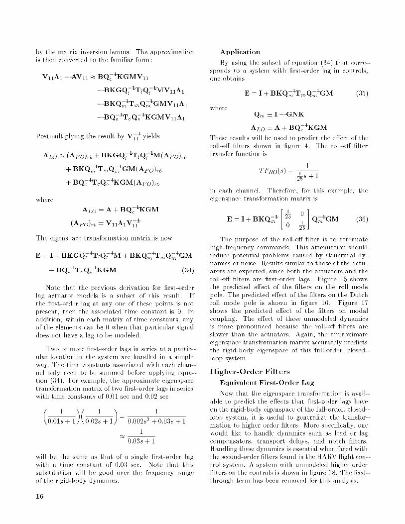
To evaluate full-order, closed-loop system dynam-ics, consider the portion of the eigenspace that cor-responds to the rigid-body system. When the un-modeled dynamics are of su�ciently higher frequencythan the low-order, closed-loop system, or they areoutside the bandwidth of the pilot, the dynamics thatare dominant to the pilot will be determined by therigid-body eigenspace. The rigid-body eigenspaceis a combination of the rigid-body eigenvalues andeigenvector elements that are associated with therigid-body modes. As an example, the rigid-bodyroll pole of the low-order, closed-loop system and ofthe 25-state system is shown in �gure 5 as a functionof angle of attack.
0
-.5
-1.0
-1.5
-2.0
-2.5
-3.0
-3.50 10 20 30
α, deg
Low-order system roll modeFull-order system roll mode
Rol
l mod
e po
le, r
ad/s
ec
40 50 60
Figure 5. Low-ordersystem and full-order,closed-loopsystem
roll pole.
The full-order, closed-loop system has dynamicsde�ned by
_x = AFOx +BFOupilot
The rigid-body eigenspace is characterized here by aspectral decomposition of AFO such that
AFOV = V�
The eigenvalue and eigenvector matrices are thenpartitioned to separate the eigenspace of interest sothat
V =
�V11 V12
V21 V22
�
� =
��1 0
0 �2
�
where �1 is a square matrix containing achievedrigid-body eigenvalues on its diagonal and V11 is asquare matrix containing achieved rigid-body eigen-vector elements associated with rigid-body states.Ideally, one would like to compare the eigenspace ofthe low-order, closed-loop system with the eigenspaceof
(AFO)rb � V11�1V�111
(i.e., the rigid-body eigenspace of the full-order,closed-loop system). This matrix has the same di-mensions as the low-order, closed-loop system matrixALO.
6

Although this reduced-order system is not a sub-
stitute for a look at frequency response and time
histories of the full-order system, it does allow the
control law designer to compare the dynamics of the
full-order, closed-loop system with well-understood
aircraft rigid-body dynamics. Also, knowledge of the
achieved rigid-body eigenspace is important because
its relationship with the desired dynamics fundamen-
tally determines whether or not certain dynamics can
be omitted from the design model.
Eigenspace Transformation Matrix
A concept that will appear repeatedly in this work
is that of a single matrix transformation in the form
ALO = E(AFO)rb
where ALO is the low-order, closed-loop system ma-
trix and (AFO)rb is composed of the rigid-body por-
tion of the full-order, closed-loop system eigenspace,
as described in the section entitled \Spectral De-
composition." The term E will be referred to
as an eigenspace transformation matrix. Although
ALO and (AFO)rb are not actually the eigenspaces,
their eigenvalues and eigenvectors are the rigid-body
eigenspace of the low- and full-order closed-loop
systems, respectively. All three of these matrices
are square, and they have dimensions equal to the
number of states in the rigid-body system. As
the unmodeled dynamics become less signi�cant to
the achieved rigid-body eigenspace, the eigenspace
transformation matrix should approach the identity
matrix.
A look at the most signi�cant contributors to
the eigenspace transformation matrix may provide
insight into what causes the rigid-body dynamics to
di�er from those of the low-order, closed-loop system.
If the e�ect on the rigid-body eigenspace can be
easily calculated, such a calculation could be useful
in determining whether certain dynamics can be left
out of the design model.
SISO Example
To facilitate the discussion of the multiple-input/
multiple-output (MIMO) results in this report, a
single-input/single-output (SISO) example is now
presented. The SISO system (�g. 6) presented is a
�rst-order roll mode approximation of the HARV at
an angle of attack of 5�. Aileron de ection is the
plant input, and roll rate is the plant output. The
�rst-order lag aileron actuator model is the unmod-
eled dynamics in this example.
upilot p
Actuatormodel
Low-orderplant
Feedbackgains
1
τail s + 1
kFB
++
Lδailδail
s - Lp
Figure 6. SISO example with �rst-order roll mode approxi-
mation at angle of attack of 5�.
For the purposes of control law design, the �rst-
order lag aileron actuator is not included in the
design model. This SISO low-order, closed-loop
design model can be written as
p(s)
upilot(s)=
L�ails� Lp� L�ailkFB
(6)
With the actuator model, this full-order, closed-loop
system has two states, and it can be written as
p(s)
upilot(s)=
L�ail(�ails + 1)(s� Lp)� L�ailkFB
(7)
In state space, this full-order, closed-loop system is
expressed as
�_p
_�ail
�=
"Lp L�ail
��1
ailkFB ���1
ail
#�p
�ail
�+
�0
��1
ail
�upilot
The low-order, closed-loop system has one state, with
the eigenvalue
�LO = Lp+ L�ailkFB (8)
which is the desired roll mode pole. The full-order,
closed-loop stability matrix is
AFO =
"Lp L�ail
��1
ailkFB ���1
ail
#
Of interest are the eigenvalues and eigenvectors of
this closed-loop system corresponding to the rigid-body dynamics, or roll mode. The eigenvalue is
�FOrb and the eigenvector is �11 when this full-order,
closed-loop system matrix is written as the spectraldecomposition�
Lp L�ail
��1
ailkFB ��
�1
ail
���11 �12
�21 �22
�=
��11 �12
�21 �22
���FOrb
0
0 �HO
�
7

Note that �FOrb and �11 are scalars and that, in theabsence of �21, �11 is arbitrary. In this development,only the upper left and lower left partitions of theabove matrix equation are needed such that
Lp�11+L�ail�21 = �11�FOrb (9)
��1
ailkFB�11� ��1
ail�21 = �21�FOrb (10)
Now, the goal is to eliminate �21 and solve for�LO in terms of �FOrb. The method that provessuccessful when working with the MIMO system isthe following. Equations (9) and (10) are rewrittenas
Lp�11� �11�FOrb= �L�ail�21 (11)
kFB�11 = �21+ �ail�21�FOrb (12)
Equation (11) is expanded into an in�nite seriessuch that each term contains the right-hand side ofequation (12). To start this expansion into an in�niteseries, add and subtract �Lp�ail�21�FOrb and groupterms to give
Lp�11� �11�FOrb=�L�ail(�21+ �ail�21�FOrb)
+L�ail�ail�21�FOrb
Continuing in a similar manner by adding andsubtracting
(�1)iL�ail�iail�21�
iFOrb
(i = 2; 3; : : : ;1)
and grouping terms to get the right-hand side ofequation (12) in each term yields the in�nite series
Lp�11� �11�FOrb= �L�
ail(�21+ �ail�21�FOrb
)
+ L�ail�ail(�21+ �ail�21�FOrb
)�FOrb
� L�ail�2
ail(�21+ �ail�21�FOrb
)�2
FOrb
+ L�ail�3
ail(�21+ �ail�21�FOrb
)�3
FOrb: : :
Then eliminate �21 by using equation (12) so that
Lp�11� �11�FOrb= �L�
ailkFB�11+L�
ail�ailkFB�FOrb
�11
�L�ail�2
ailkFB�
2
FOrb�11
+L�ail�3
ailkFB�
3
FOrb�11 : : :
Dividing out the now arbitrary �11, the abovebecomes
Lp� �FOrb= �L�
ailkFB+L�
ail�ailkFB�FOrb
�L�ail�2
ailkFB�
2
FOrb+ L�
ail�3
ailkFB�
3
FOrb: : :
One can now relate the low-order (eq. (8)) and full-order, closed-loop rigid-body pole as
�LO = �FOrb+L�ail�ailkFB�FOrb
�L�ail�2
ailkFB�
2
FOrb+L�ail�
3
ailkFB�
3
FOrb: : :
This is an in�nite series that converges as long as
j�ail�FOrbj < 1
In the case where the actuator has a muchlower time constant than the rigid-body modej�ail�FOrbj � 1, the �rst two terms constitute a goodapproximation to the in�nite series such that
�LO ��1 +L�ail�ailkFB
��FOrb
or
�FOrb�b�FOrb�
�1 + L�ail�ailkFB
��1
�LO
where b�FOrb denotes an approximation of �FOrb. Aplot of this approximation is shown in �gure 7. Note
that b�FOrb approximates �FOrb up to an actuatortime constant of approximately 0.06 sec, which isthree times slower than the actual actuator timeconstant.
.5
.4
.3
.2
.1
0 .04 .08 .12 .16 .20Open-loop actuator time constant, sec
Complexpair formed
Closed-loopactuator pole
Tim
e co
nsta
nt, s
ec
-λ-1LO
-λ-1FOrb-λ
-1FOrb
Figure 7. E�ect of �rst-order actuator model on SISO system
and approximation.
Because of the divergence of ��1
LOand ��1
FOrb, a
point will exist where the open-loop actuator timeconstant is high enough that it becomes necessaryto include this actuator model in the design process.This point will be determined by the required levelof accuracy in the �nal design. A point will alsoexist where the rigid-body roll mode and the actuator
8

mode couple together to form a single oscillatorymode.
Approximating the Transformation
First-Order Actuators
In this section, an approximation of the eigen-space transformation is derived and tested for un-modeled dynamics placed at the input of the rigid-body aircraft. The eigenspace transformation relatesthe rigid-body eigenspace of the low-order, closed-loop system used for the design with the full-order,closed-loop system. Here, the SISO results shown inthe section entitled \SISO Example" are generalizedfor �rst-order lag actuator dynamics applied to theMIMO design.
Without feed-through term. Consider thefollowing system, shown in �gure 8, which representsthe HARV rigid-body system and the �rst-order lagactuator models:
_x = Ax +Bv (System dynamics)
z =Mx (System measurements)
Te _v = �v + u (Actuator dynamics)
u = KGz+Kupilot (Control law)
(13)
upilot u v z
Feed-forwardgains
Low-ordersystemActuators
Feedbackgains
1
τis + 1K
G
++
A, B,M
Figure 8. System block diagram with �rst-order lag actuators
as unmodeled dynamics.
The measurement feed-through term is omitted fromthis derivation for clarity. The actuator matrix isdiagonal and contains the time constant associatedwith each actuator:
Te �
264�1 0
. . .
0 �e
375
This formulation corresponds to actuator dynamicswith the transfer functions
vi(s)
ui(s)=
1
�is+ 1(i = 1; 2; : : : ; e)
This full-order, closed-loop system now has n + e
states with dynamics expressed as
�_x
_v
�=
�A B
T�1e KGM �T
�1e
��x
v
�+
�0
T�1e K
�upilot
z = [M 0]
�x
v
�
The closed-loop stability matrix for the low-ordersystem is
ALO = A+BKGM
and the closed-loop stability matrix for this full-ordersystem is
AFO =
�A B
T�1e KGM �T
�1e
�
Of interest are the eigenvectors and eigenvalues ofthis closed-loop system corresponding to the rigid-body dynamics. These correspond to V11 and �1
when this full-order system matrix is rewritten asthe spectral decomposition,
�A B
T�1eKGM �T
�1e
��V11 V12
V21 V22
�=
�V11 V12
V21 V22
���1 0
0 �2
�
(14)
Here, we need only the upper left and lower leftpartitions of the above matrix equation, or
AV11+BV21 = V11�1 (15)
T�1e KGMV11�T
�1e V21 = V21�1 (16)
or equivalently,
V11�1 �AV11 = BV21 (17)
KGMV11 = V21+TeV21�1 (18)
As an intermediate step to obtain the eigenspacetransformation approximation, equation (17) is ex-panded as an in�nite series. To generate this series,add and subtract BTeV21�1 and group terms cor-responding to the right-hand side of equation (18).This becomes
V11�1�AV11 = B(V21+TeV21�1)�BTeV21�1
Then add and subtract BT2eV21�
21 and group as
before such that
V11�1�AV11 = B(V21+TeV21�1)�BTe(V21
+TeV21�1)�1+BT2eV21�
21
9

where A2� AA, A3
� AAA; : : : Continuing toadd and subtract BTi
eV21�i1 (i = 3; 4; : : : ;1) and
following the same grouping strategy yields the fol-lowing in�nite series:
V11�1�AV11 = B(V21+TeV21�1)
�BTe(V21+TeV21�1)�1
+BT2e(V21+TeV21�1)�
21
�BT3e(V21+TeV21�1)�
31 + : : :
Equation (18) can now be substituted into each termon the right to get
V11�1 �AV11 = BKGMV11�BTeKGMV11�1
+BT2eKGMV11�
21 � : : : (19)
Postmultiply equation (19) by V�111 . The in�niteseries that results relates the rigid-body eigenspaceof the low-order, closed-loop system with that of thefull-order, closed-loop system in which
ALO = (AFO)rb +BTeKGM(AFO)rb
�BT2eKGM(AFO)
2rb
+BT3eKGM(AFO)
3rb� : : : (20)
where
(AFO)rb = V11�1V�111
as de�ned in the section entitled \SpectralDecomposition."
As the amount of augmentation increases (Kand G), the e�ect of the unmodeled dynamics on therigid-body dynamics is increased. As the actuatorsget faster (i.e., as the elements of Te approach 0) thee�ect on the closed-loop eigenspace is decreased. Theeigenspace of the low-order, closed-loop system andthe rigid-body eigenspace of the full-order, closed-loop system become equal.
The convergence of equation (19) is equivalent tothe convergence of
1Xi=0
(�1)iTieKGMV11�
i1
This series can be bounded using the matrix 2-normand the Schwarz inequality (ref. 8) such that
kTieKGMV11�
i1k � kTek
ikKGMV11k k�1ki
(i = 0; 1; : : : ;1)
The matrix 2-norm of A equals max �(AA�)1=2. Byvirtue of being eigenvectors, V11 can be multipliedby an arbitrary scalar. This factor is chosen suchthat the matrix norm of KGMV11 is unity, so that
kTieKGMV11�
i1k � (kTek k�1k)
i
Convergence of equation (19) is therefore guaranteedwhen
kTek k�1k < 1
Feed-through term. For many systems, the low-order model of interest may have a feed-through orNmatrix term. This is the case for the HARV controllaw design. Here, the previous analysis and thedevelopment are extended to obtain the eigenspacetransformation matrix for this type system. Tobegin, consider the system that represents an aircraftwith �rst-order lag actuator models in which
_x = Ax+Bv (System dynamics)
z =Mx+Nv (System measurements)
Te _v = �v + u (Actuator dynamics)
u = KGz+Kupilot (Control law)
The system has n + e states, with the closed-loopdynamics
�_x
_v
�=
�A B
T�1e KGM T�1e KGN �T�1e
��x
v
�
+
�0
T�1e K
�upilot
z = [M N]
�x
v
�
The spectral decomposition of the system matrix is
�A B
T�1e KGM T�1e KGN�T�1e
� �V11 V12
V21 V22
�
=
�V11 V12
V21 V22
� ��1 0
0 �2
�
where �1 and V11 correspond to the rigid-bodyeigenspace. As before, only the upper left and lowerleft partitions of this equation are used, or
V11�1 �AV11 = BV21 (21)
KGMV11 = QeV21+TeV21�1 (22)
whereQe � I�KGN
10

This is a useful de�nition for the development tofollow, since from the section entitled \Low-Order,Closed-Loop System"
ALO = A+BQ�1e KGM
As in the previous section, equation (21) is ex-panded as an in�nite series with terms grouped tomatch the right-hand side of equation (22). Theseries is generated as before: add and subtractBQ�1e TeV21�1 to equation (21), so that
V11�1�AV11 = BQ�1e (QeV21+TeV21�1)
�BQ�1e TeV21�1
Then continue in a similar manner as before andapply equation (22) as follows:
V11�1�AV11=BKGMV11�BQ�1
eTeQ
�1
eKGMV11�1
+BQ�1eTeQ
�1
eTeQ
�1
eKGMV11�
2
1� : : :
Convergence is guaranteed when kQ�1e Tek k�1k < 1.
To obtain the �nal form, postmultiply by V�111
, sothat
ALO = (AFO)rb+BQ�1
e TeQ�1
e KGM(AFO)rb
�BQ�1e TeQ�1
e TeQ�1
e KGM(AFO)2
rb+ : : : (23)
An important simpli�cation of equation (23) is
suggested by multiplying through by (AFO)�1rb
, sothat
ALO(AFO)�1
rb= I+BQ�1e TeQ
�1
e KGM
�BQ�1e TeQ�1
e TeQ�1
e KGM(AFO)rb+ : : :
The 2-norm of each successive term on the right-handside, except the identity term, is shown in �gure 9.Clearly, the �rst two terms constitute a reasonableapproximation to the in�nite series for this example.
An advantage of using the �rst two terms as anapproximation to the series is the following predic-tion of the rigid-body eigenspace of the full-order,closed-loop system expressed in terms of the low-order, closed-loop system:
(AFO)rb � (I+BQ�1e TeQ�1e KGM)�1ALO
1.0
.8
.6
.4
.2
0 10 20 30α, deg
Second termThird termFourth term
2-no
rm o
f te
rms
in in
fini
te s
erie
s
40 50 60
Figure 9. 2-norm of terms in in�nite series.
This expression leads to the concept of a singlematrix (an eigenspace transformation matrix) whichtransforms the low-order, closed-loop stability matrixto approximate the rigid-body eigenspace of the full-order, closed-loop system such that
(AFO)rb � E�1ALO (24)
For this full-order, closed-loop system, the eigenspacetransformation matrix is simply
E = I+BQ�1e TeQ�1e KGM
Application
The results of the previous development are ap-plied to the HARV lateral-directional ight controlsystem design. The validity of the previous analysisin predicting the e�ect of �rst-order actuator modelson the rigid-body dynamics is shown. The low-ordersystem was used to generate the feedback gains. Be-cause there are four measurements, the rigid-bodypoles are exactly placed. Moreover, the low-order,closed-loop eigenspace is the desired eigenspace.
In this example, the actuators are modeled as thefollowing transfer functions:
TFail(s) =1
148s+ 1
TFrud(s) =1
140s+ 1
TFas(s) =1
130s+ 1
TFytv(s) =1
148s+ 1
TFrtv(s) =1
148s+ 1
11

The approximate eigenspace transformation matrixis then
E = I+BQ�1e
26666664
1
480
1
40
1
30
1
48
0 1
48
37777775Q�1e KGM
(25)
The expression E�1ALO is postulated to be an ap-proximation to the rigid-body eigenspace of the full-order, closed-loop system (i.e., V11�1V
�1
11).
The �rst check on the validity of the approxima-tion will be on the convergence of the in�nite seriesused to derive the eigenspace transformation matrix.The test
kQ�1e Tek k�1< 1
is applied using the 2-norm. At an angle of attack of20�, the left side of the equation is equal to 0.0737.This value indicates convergence of the series.
To examine the range in which the eigenspacetransformation matrix is valid, the poles of the ac-tuators are gradually slowed down. This procedureis done by multiplying the actuator poles by a reduc-tion factor k which is varied from 1 to 0 such that
T�1slow
= kT�1e
whereTslow
_v = �v + u
The error associated with using this eigenspace trans-formation matrix in predicting the roll mode poleand Dutch roll natural frequency for a ight condi-tion with an angle of attack of 20� is shown in �g-ure 10. The actuators have been slowed by a factorof 5 when the aileron actuator and the roll mode polesform an oscillatory pair. The unmodeled dynamicswill need to be much closer in frequency to the low-order, closed-loop system for there to be a problemwith the assumptions made.
Figure 11 shows how well E�1ALO predicts therigid-body roll mode pole. The low-order characteris-tics are those of the design model, and they representplaced dynamics. The full-order characteristics arethose of the low-order plant plus the actuator dy-namics. The predicted characteristics are obtainedfrom equation (24), and they are expected to predictthe full-order characteristics. The Dutch roll modepole is shown in �gure 12. Note that the variation ofthe roll mode and Dutch roll frequencies are capturedalong with the variation in Dutch roll damping. The
-1.6Low orderFull-order rigid bodyPredicted rigid body
1.0 0.8 0.6 0.4 0.2 0
-2.0
-2.4
-2.8
-3.2
k
1.0 0.8 0.6 0.4 0.2 0k
Rol
l mod
e po
le, r
ad/s
ec
3.0
2.5
2.0
1.5
1.0
.5
0Dut
ch r
oll n
atur
al f
requ
ency
, rad
/sec
Figure 10. Plots that verify accuracy of eigenspace transfor-
mation matrix approximationwith angle of attack of 20�.
-.5
-1.0
-1.5
-2.0
-2.5
-3.0
-3.5100 20 30
Low orderWith actuatorsPredicted
α, deg
Rol
l mod
e po
le, r
ad/s
ec
40 50 60
Figure 11. Roll mode pole prediction with actuator models.
12

2.4
2.2
2.0
1.8
1.6
1.4
1.2
1.0
.80 10 20 30
α, deg40 50 60
.82
.78
.74
.70
.66
.620 10 20 30
α, deg
Dut
ch r
oll d
ampi
ng r
atio
Dut
ch r
oll n
atur
al f
requ
ency
, rad
/sec
40 50 60
Low orderWith actuatorsPredicted
Figure 12. Dutch roll mode pole prediction with actuator
models.
negligible variation of the spiral mode pole, whichis not shown, is also captured by the approximation.
For all cases, the approximate eigenspace transforma-
tion matrix accurately predicts the rigid-body poles
of the full-order, closed-loop system.
The predicted e�ect of actuators on the desired
eigenvector elements is shown in �gure 13. The �rst
of these elements is the �-to-� ratio in the Dutch rollmode. The second element is the �-to-p ratio in the
roll mode. The magnitude of the ratio of each of these
two eigenvector elements is shown. These ratios give
an indication of how much the roll and Dutch roll
modes are coupled. The low-order �-to-p ratio in theroll mode is 0 for all cases. The low-order �-to-� ratio
in the Dutch roll mode coincides with that of the
full-order, closed-loop system. The �-to-p ratio is in
seconds, and the �-to-� ratio is nondimensional. The
eigenvectors appear to be a�ected considerably less
0
1
2
3
4
5
6
10 20
Low orderWith actuatorsPredicted
30α, deg
40 50 60
0
.004
.008
.012
.016
.020
10 20 30α, deg
β-to
-p r
atio
in
roll
mod
e ei
genv
ecto
r, s
ecφ-
to-β
rat
io in
D
utch
rol
l eig
enve
ctor
40 50 60
Figure 13. Eigenvector prediction with actuator models.
than the eigenvalues by unmodeled dynamics. Thisresult will show up repeatedly in the examples that
are presented. Again, the approximate eigenspace
transformation matrix accurately predicts the full-
order, closed-loop rigid-body eigenspace.
Dynamics in Other Locations
General Form of Eigenspace
Transformation Matrix
One would like a general expression for the
eigenspace transformation matrix for dynamics at
other points, including the input to the plant, in the
control system structure. It is possible to constructthe system with a �rst-order lag at three locations
within this system. The eigenspace transformation
matrix for a �rst-order lag in any or all of these loca-
tions will then be readily available from the general
form.
13

upilot
uFB
uc vm
vl
ve z
Feed-forwardgains
Low-ordersystem
Feedbackgains
Tm Te
G Tl
Ku
++
A, B,M, N
Figure 14. System block diagramwith �rst-order lags in three
locations.
Consider the system shown in �gure 14, in which
_x = Ax+Bve Te _ve = �ve + u
u = Kvm Tm _vm = �vm+ uc
uFB = Gvl Tl _vl = �vl + z
z =Mx+Nve uc = uFB + upilot
where x 2 Rn, ve 2 R
e, vm 2 Rm, and vl 2
Rl. When the equations governing this system are
combined, the full-order, closed-loop system becomes
8>><>>:
_x
_ve
_vm
_vl
9>>=>>;
=
2664
A B 0 0
0 �T�1e
T�1eK 0
0 0 �T�1m
T�1mG
T�1lM T�1
lN 0 �T�1
l
3775
8>><>>:
x
ve
vm
vl
9>>=>>;
+
8>><>>:
0
0
T�1m
0
9>>=>>;upilot
with n+e+m+ l states. The spectral decompositionof the system matrix becomes
26664
A B 0 0
0 �T�1e T�1e K 0
0 0 �T�1m T�1
m G
T�1lM T�1
lN 0 �T�1
l
37775
26664V11 V12
V21 V22
V31 V32
V41 V42
37775
=
26664V11 V12
V21 V22
V31 V32
V41 V42
37775��1 0
0 �2
�(26)
where V11 and �1 are the eigenvector elements andeigenvalues associated with the rigid-body eigenspaceof the full-order, closed-loop system, respectively.
The eigenvector matrix has been partitioned suchthat the �rst-column partition contains n columns,and the second contains e+m+l columns. The �rst-,second-, third-, and fourth-row partitions contain n,e, m, and l rows, respectively. Equations in the �rst-column partition of the matrix equation (26) are
V11�1 �AV11 = BV21 (27)
KV31 = V21+TpV21�1 (28)
GV41 = V31+TmV31�1 (29)
MV11 = �NV21+V41+TlV41�1 (30)
To get the feed-through term in a useful form, asecond version of equations (28), (29), and (30) isneeded, so that
KV31 = QeV21+TeV21�1 +KGNV21 (31)
GV41 = QmV31+TmV31�1 +GNKV31 (32)
MV11 = QlV41+TlV41�1 +NKGV41�NV21
(33)where
Qe � I�KGN
Qm � I�GNK
Ql � I�NKG
As in the previous development, expansion ob-tained via adding and subtracting needed terms willturn equations (27) through (30) into an in�nite se-ries. It is again assumed that the speed of the un-modeled dynamics is faster than that of the low-order, closed-loop system. Hence, each new term ofthe series will be smaller than its predecessor. Toform an analogous approximation to the series, allterms containing two or more time constant matricesand two or more eigenvalue matrices will be dropped.Expand equation (27) so that equation (31) can beused; thus,
V11�1�AV11=BQ�1e(QeV21+TeV21�1)
�BQ�1eTeQ
�1e(QeV21+TeV21�1)�1
+BQ�1eTeQ
�1eTeQ
�1e(QeV21
+TeV21�1)�21� : : :
Then apply equation (31) and drop the terms withhigher powers of Te and �1, so that
V11�1�AV11�BQ�1e(KV31�KGNV21)
�BQ�1eTeQ
�1e
(KV31�KGNV21)�1
For the remainder of the development, this equationwill be stated as an approximation; all terms with
14

more than a single appearance of T and �1 will bedropped as they occur.
Expand the above equation again so that theright-hand side of equation (29) appears as
V11�1�AV11�BQ�1
eK(V31+TmV31�1�GNV21)
�BQ�1eKTmV31�1
�BQ�1eTeQ
�1
eK(V31+TmV31�1
�GNV21)�1
Then by equation (29),
V11�1�AV11� BQ�1
eK(GV41�GNV21)
�BQ�1eKTmV31�1
�BQ�1eTeQ
�1
eK(GV41�GNV21)�1
Equation (32) will now be used to eliminate the lastV31 term, so that
V11�1�AV11� BQ�1
eKG(V41�NV21)
�BQ�1eKTmQ
�1
m(QmV31+TmV31�1)�1
�BQ�1eTeQ
�1
eKG(V41�NV21)�1
and then
V11�1�AV11� BQ�1
eKG(V41�NV21)
�BQ�1eKTmQ
�1
mG(V41�NKV31)�1
�BQ�1eTeQ
�1
eKG(V41�NV21)�1
Equation (28) is then used; thus,
V11�1�AV11� BQ�1
eKG(V41�NV21)
�BQ�1eKTmQ
�1
mG(V41�NV21)�1
�BQ�1eTeQ
�1
eKG(V41�NV21)�1
Expand the above equation again so that theright-hand side of equation (30) will allow V41 tobe eliminated:
V11�1�AV11�BQ�1
eKG(V41+TlV41�1
�NV21)�BQ�1
eKGT
lV41�1
�BQ�1eKTmQ
�1
mG(V41+TlV41�1
�NV21)�1�BQ�1
eTeQ
�1
eKG(V41
+TlV41�1�NV21)�1
Then apply equation (30), so that
V11�1�AV11 � BQ�1eKGMV11
�BQ�1eKGT
lV41�1
�BQ�1eKTmQ
�1mGMV11�1
�BQ�1eTeQ
�1eKGMV11�1
Next expand the above expression so that equa-tion (33) is used and
V11�1�AV11�BQ�1
eKGMV11
�BQ�1eKGT
lQ�1l(V41+TlV41�1)�1
�BQ�1eKTmQ
�1
mGMV11�1
�BQ�1eTeQ
�1
eKGMV11�1
or
V11�1�AV11�BQ�1
eKGMV11
�BQ�1eKGT
lQ�1l(MV11�NKGV41
+NV21)�1�BQ�1
eKTmQ
�1
mGMV11�1
�BQ�1eTeQ
�1
eKGMV11�1
Equations (29) and (28) are subsequently applied toeliminate the last V41 term; thus,
V11�1�AV11�BQ�1
eKGMV11
�BQ�1eKGT
lQ�1l(MV11�NV21
+NV21)�1�BQ�1
eKTmQ
�1
mGMV11�1
�BQ�1eTeQ
�1
eKGMV11�1
All unwanted terms are eliminated, so that
V11�1�AV11�BQ�1
eKGMV11
�BQ�1eKGT
lQ�1lMV11�1
�BQ�1eKTmQ
�1
mGMV11�1
�BQ�1eTeQ
�1
eKGMV11�1
Finally, note that
Q�1eKG= (I�KGN)
�1KG=KG(I�NKG)�1
=KGQ�1l
Q�1eK= (I�KGN)
�1K=K(I�GNK)�1
=KQ�1m
15
by the matrix inversion lemma. The approximationis then converted to the familiar form:
V11�1 �AV11 � BQ�1e KGMV11
�BKGQ�1lTlQ
�1
lMV11�1
�BKQ�1m TmQ�1
m GMV11�1
�BQ�1e TeQ�1
e KGMV11�1
Postmultiplying the result by V�111
yields
ALO � (AFO)rb +BKGQ�1lTlQ
�1
lM(AFO)rb
+BKQ�1m TmQ�1
m GM(AFO)rb
+BQ�1e TeQ�1
e KGM(AFO)rb
where
ALO = A+BQ�1e KGM
(AFO)rb = V11�1V�1
11
The eigenspace transformation matrix is now
E = I+BKGQ�1lTlQ
�1
lM+BKQ�1m TmQ
�1
m GM
+BQ�1e TeQ�1
e KGM (34)
Note that the previous derivation for �rst-orderlag actuator models is a subset of this result. Ifthe �rst-order lag at any one of these points is notpresent, then the associated time constant is 0. Inaddition, within each matrix of time constants, anyof the elements can be 0 when that particular signaldoes not have a lag to be modeled.
Two or more �rst-order lags in series at a partic-ular location in the system are handled in a simpleway. The time constants associated with each chan-nel only need to be summed before applying equa-tion (34). For example, the approximate eigenspacetransformation matrix of two �rst-order lags in serieswith time constants of 0.01 sec and 0.02 sec
�1
0:01s+ 1
��1
0:02s+ 1
�=
1
0:002s2 + 0:03s+ 1
�
1
0:03s+ 1
will be the same as that of a single �rst-order lagwith a time constant of 0.03 sec. Note that thissubstitution will be good over the frequency rangeof the rigid-body dynamics.
Application
By using the subset of equation (34) that corre-sponds to a system with �rst-order lag in controls,one obtains
E = I+BKQ�1m TmQ�1
m GM (35)
whereQm � I�GNK
ALO = A+BQ�1e KGM
These results will be used to predict the e�ect of theroll-o� �lters shown in �gure 4. The roll-o� �ltertransfer function is
TFRO(s) =1
1
25s + 1
in each channel. Therefore, for this example, theeigenspace transformation matrix is
E = I+BKQ�1m
"1
250
0 1
25
#Q�1m GM (36)
The purpose of the roll-o� �lter is to attenuatehigh-frequency commands. This attenuation shouldreduce potential problems caused by structural dy-namics or noise. Results similar to those of the actu-ators are expected, since both the actuators and theroll-o� �lters are �rst-order lags. Figure 15 showsthe predicted e�ect of the �lters on the roll modepole. The predicted e�ect of the �lters on the Dutchroll mode pole is shown in �gure 16. Figure 17shows the predicted e�ect of the �lters on modalcoupling. The e�ect of these unmodeled dynamicsis more pronounced because the roll-o� �lters areslower than the actuators. Again, the approximateeigenspace transformation matrix accurately predictsthe rigid-body eigenspace of this full-order, closed-loop system.
Higher-Order Filters
Equivalent First-Order Lag
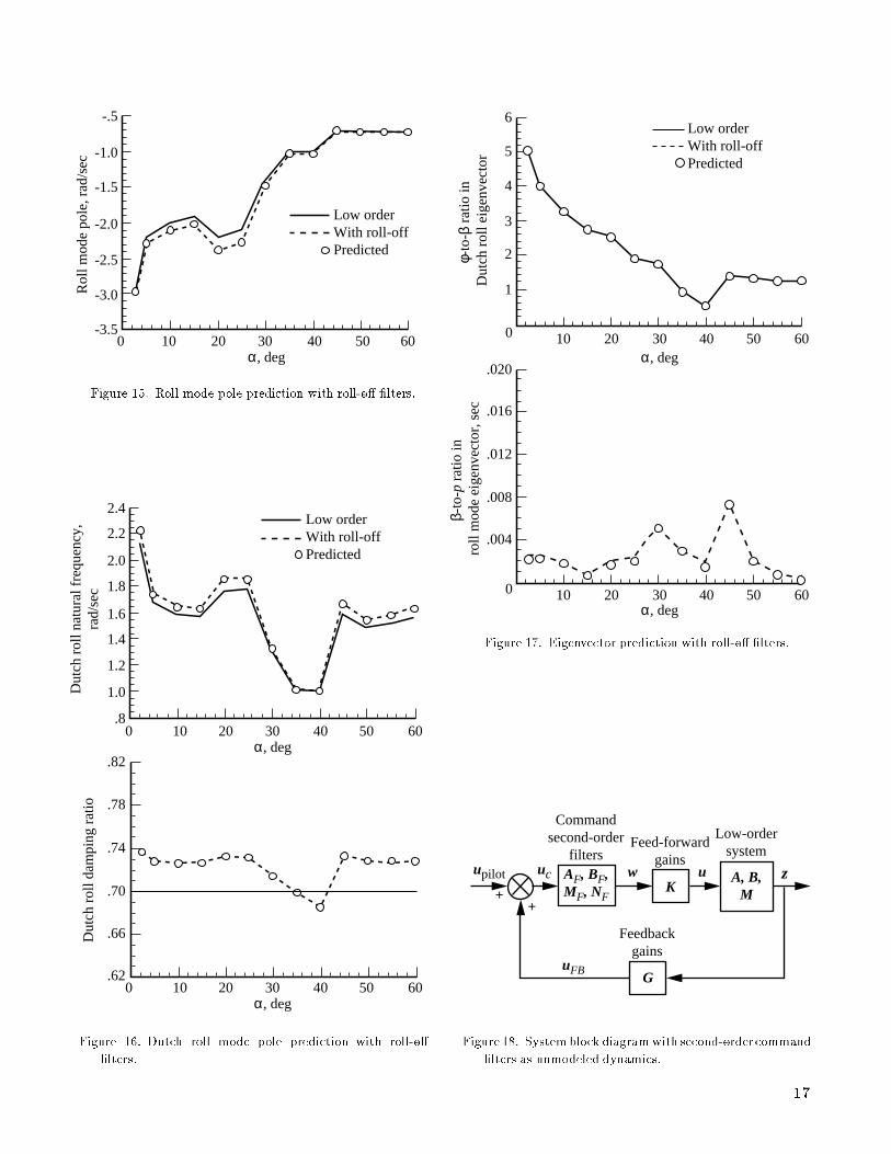
Now that the eigenspace transformation is avail-able to predict the e�ects that �rst-order lags haveon the rigid-body eigenspace of the full-order, closed-loop system, it is useful to generali ze the transfor-mation to higher order �lters. More speci�cally, onewould like to handle dynamics such as lead or lagcompensators, transport delays, and notch �lters.Handling these dynamics is essential when faced withthe second-order �lters found in the HARV ight con-trol system. A system with unmodeled higher order�lters on the controls is shown in �gure 18. The feed-through term has been removed for this analysis.
16
-.5
Low orderWith roll-offPredicted
-1.0
-1.5
-2.0
-2.5
-3.0
-3.50 10 20 30
α, deg
Rol
l mod
e po
le, r
ad/s
ec
40 50 60
Figure 15. Roll mode pole prediction with roll-o� �lters.
2.4Low orderWith roll-offPredicted
2.2
2.0
1.8
1.6
1.4
1.2
1.0
.80 10 20 30
α, deg
Dut
ch r
oll n
atur
al f
requ
ency
,ra
d/se
c
40 50 60
.82
.78
.74
.70
.66
.620 10 20 30
α, deg
Dut
ch r
oll d
ampi
ng r
atio
40 50 60
Figure 16. Dutch roll mode pole prediction with roll-o�
�lters.
6
5
Low orderWith roll-offPredicted
4
3
2
1
0 10 20 30α, deg
40 50 60
.020
.016
.012
.008
.004
0 10 20 30α, deg
40 50 60
β-to
-p r
atio
in
roll
mod
e ei
genv
ecto
r, s
ecφ-
to-β
rat
io in
D
utch
rol
l eig
enve
ctor
Figure 17. Eigenvector prediction with roll-o� �lters.
upilot
uFB
uc z
Feed-forwardgains
Low-ordersystem
Commandsecond-order
filters
Feedbackgains
G
Kuw
++
A, B,M
AF, BF,MF, NF
Figure 18. Systemblock diagramwith second-ordercommand
�lters as unmodeled dynamics.
17

The system can be written as follows:
_x = Ax+BKw (System dynamics/
feed-forward gains)
z =Mx (System measurements)
uFB = Gz (Feedback control)
uc = uFB + upilot (Feed-forward control)
_v = AFv +BFuc (Filter system dynamics)
w =MFv +NFuc (Filter measurements)
where the �lters in parallel channels are realized as
AF =
264Af1
0
. . .
0 Afm
375
BF =
264Bf1
0
. . .
0 Bfm
375
MF =
264Mf1
0
. . .
0 Mfm
375
NF =
264Nf1
0
. . .
0 Nfm
375
thus giving each higher order �lter a transfer functionof the form
Mfi
�sI�Afi
��1Bfi
+Nfi(i = 1; 2; : : : ; m)
The closed-loop system matrix spectral decompo-sition for this system is
�A+BKNFGM BKMF
BFGM AF
� �V11 V12
V21 V22
�
=
�V11 V12
V21 V22
� ��1 0
0 �2
�
where again �1 and V11 correspond to the rigid-body eigenspace. When multiplied out, this equationyields four matrix equations. Two of these equations,which correspond to the upper left and lower leftpartitions, can be written as
V11�1�(A+BKNFGM)V11 = BKMFV21 (37)
�A�1F BFGMV11 = V21�A
�1F V21�1 (38)
where it is assumed that the higher order �lters haveno poles at the origin. Equation (37) is expanded bymethods used in previous sections to yield the in�niteseries
V11�1�AV11�BKNFGMV11
=BKMF(V21�A�1
FV21�1)+BKMFA
�1
F(V21
�A�1
FV21�1)�1+BKMFA
�2
F(V21�A
�1
FV21�1)�
2
1+ : : :
Substituting equation (38) yields
V11�1�AV11�BKNFGMV11
=�BKMFA�1
FBFGMV11
�BKMFA�2
FBFGMV11�1�BKMFA
�3
FGMV11�
2
1� : : :
Postmultiplying by V�111 , we get
(AFO)rb = A+BKNFGM�BKMFA�1
FBFGM
�BKMFA�2
FBFGM(AFO)rb
�BKMFA�3
FBFGM(AFO)
2
rb� : : : (39)
The type of higher order �lters considered isrestricted to those with a steady-state gain of 1through all channels. The steady-state gain is thelimit of the �lter transfer function as s goes to 0.This gain of 1 yields the relations
�MfiA�1fiBfi
+Nfi= 1
or
�MFA�1F BF +NF = I
Using this result to combine the �rst three terms onthe right-hand side of equation (39), we get
ALO = (AFO)rb +BKMFA�2FBFGM(AFO)rb
+BKMFA�3FBFGM(AFO)
2rb+ : : : (40)
The approximate eigenspace transformation matrixof any higher order �lter with a steady-state gain of1 is the same as that of a �rst-order lag with an equiv-alent time constant matrix equal to MFA
�2F BF .
Second-order �lter. A second-order �lter mod-eled as the transfer function
wi(s)
ui(s)=
!2deni
!2numi
s2 + 2�numi!numis+ !
2numi
s2 + 2�deni!denis+ !2deni
!
18
has the following system matrices
Afi=
"0 �!2
deni
1 �2�deni
!deni
#(i = 1; 2; : : : ; m)
Bfi=
!2deni
!2numi
"!2numi
� !2deni
2��numi
!numi� �
deni!deni
�#
Mfi= [0 1]
Nfi=
!2deni
!2numi
The equivalent time constant is MfiA�2fiBfi
or
�i = 2
�deni
!deni
�
�numi
!numi
!(41)
As an example, consider a notch �lter with a de-nominator damping ratio of 0.7, a numerator damp-ing ratio of 0.1, and equal natural frequencies inthe numerator and the denominator. From equa-tion (41), we see that the e�ect of the �lter on therigid-body eigenspace will be virtually the same asthat of a �rst-order lag with a break frequency of83 percent of the natural frequency of the notch �lter.
Time delay. The �rst-order Pad�e approxima-tion to a transport delay is written as
wi(s)
ui(s)=
1��tdi=2
�s
1 +�tdi=2
�s
The system matrices can be written as
Afi=�2
tdiBfi
=4
tdi
Mfi= 1 Nfi
= �1
The appropriate �rst-order lag for this transfer func-tion is found to have a time constant equal to thetransport delay magnitude such that
�i = tdi
Lead/lag compensator. Another type of �lterthat has been considered is a lead/lag compensatorof the form
wi(s)
ui(s)=
�numis+ 1
�deni
s+ 1
or in state-space form
Afi=�1
�deni
Bfi=
�deni
� �numi
�2deni
Mfi= 1 Nfi
=�numi
�deni
The rigid-body eigenspace of the full-order, closed-loop system that includes this �lter can be accuratelypredicted using the eigenspace transformation ma-trix corresponding to a �rst-order lag with a timeconstant of
�i = �deni
� �numi
This result implies that such a compensator could bedesigned to cancel much of the e�ect of unmodeleddynamics on the rigid-body eigenspace.
Application
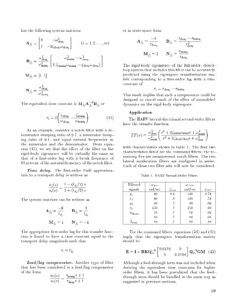
The HARV lateral-directional second-order �ltershave the transfer function
TF (s) =!2den
!2num
s2 + 2�num!nums+ !2
num
s2+ 2�den
!den
s+ !2den
!
with characteristics shown in table 1. The �rst twocharacteristics listed are the command �lters ; the re-maining �ve are measurement notch �lters. The twolateral acceleration �lters are con�gured in series.Each of these two �lter sets will now be considered.
Table 1. HARV Second-Order Filters
Filtered !den
, !num,
signals rad/sec �den
rad/sec �num
_pc 40 0.6 140 0.74
_rc 40 .6 140 .74
pb 80 .7 80 .08
rb 150 .7 150 .08
nysens 58 .7 58 .08
80 .7 80 .08_�sens 80 .7 80 .10
For the command �lters, equations (34) and (41)imply that the eigenspace transformation matrixshould be
E = I+BKQ�1m
�0:0194 0
0 0:0194
�Q�1mGM (42)
Although a feed-through term was not included whenderiving the equivalent time constants for higherorder �lters, it has been postulated that the feed-through term should be handled in the same way assuggested in previous sections.
19

-.5
-1.0
-1.5
-2.0
-2.5
-3.0
-3.5100 20 30
α, deg
Rol
l mod
e po
le, r
ad/s
ec
40 50 60
Low orderWith command filterPredicted
Figure 19. Roll mode pole prediction with command second-
order �lters.
2.4
2.0
2.2
1.8
1.6
1.2
1.0
1.4
.80 10 20 30
α, deg
Dut
ch r
oll n
atur
al f
requ
ency
, rad
/sec
40 50 60
.82
.78
.74
.70
.66
0.62
10 20 30α, deg
Dut
ch r
oll d
ampi
ng r
atio
40 50 60
Low orderWith command filterPredicted
Figure 20. Dutch roll mode pole prediction with command
second-order �lters.
6
5
4
3
2
1
0 10 20 30α, deg
40 50 60
.020
.016
.012
.008
.004
0 10 20 30α, deg
40 50 60
Low orderWith command filterPredicted
β-to
-p r
atio
in
roll
mod
e ei
genv
ecto
r, s
ecφ-
to-β
rat
io in
D
utch
rol
l eig
enve
ctor
Figure 21. Eigenvector prediction with command second-
order �lters.
From the previous discussion, these second-ordercommand �lters, having zeros with frequencies of140 rad/sec and poles with frequencies of 40 rad/sec,will a�ect the rigid-body eigenspace of the full-order,closed-loop system in the same manner as a roll-o� �lter with a time constant of 0.0194 sec. Theeigenspace results are shown in �gures 19, 20, and 21.Again, the approximate eigenspace transformationmatrix accurately predicts the resulting rigid-bodyeigenspace.
The second-order �lters in the measurement loopare notch �lters designed to cancel resonant peaksin the structural model. There are two second-order �lters in series for the nysens
channel, so theapproximate time constant associated with each willbe summed to approximate the e�ect of both. Theeigenspace transformation matrix associated with the
20

-.5
-1.0
-1.5
-2.0
-2.5
-3.0
-3.5100 20 30
α, deg
Rol
l mod
e po
le, r
ad/s
ec
40 50 60
Low orderWith measurement notchPredicted
Figure 22. Roll mode pole prediction with measurementnotch
�lters.
2.4
2.0
2.2
1.8
1.6
1.2
1.0
1.4
.80 10 20 30
α, deg
Dut
ch r
oll n
atur
al f
requ
ency
, rad
/sec
40 50 60
.82
.78
.74
.70
.66
0.62
10 20 30α, deg
Dut
ch r
oll d
ampi
ng r
atio
40 50 60
Low orderWith measurement notchPredicted
Figure 23. Dutch roll mode pole predictionwithmeasurement
notch �lters.
6
5
4
3
2
1
0 10 20 30α, deg
40 50 60
.020
.016
.012
.008
.004
0 10 20 30α, deg
40 50 60
Low orderWith measurement notchPredicted
β-to
-p r
atio
in
roll
mod
e ei
genv
ecto
r, s
ecφ-
to-β
rat
io in
D
utch
rol
l eig
enve
ctor
Figure 24. Eigenvector prediction with measurement notch
�lters.
measurement notch �lters is, from equations (34)and (41),
E= I+BKGQ�1l
2640:0155 0
0:0083
0:0369
0 0:0150
375Q�1l
M
(43)
The e�ects of these notch �lters are shown in �g-ures 22, 23, and 24. The eigenvalues and eigenvectorsof E�1ALO predict very well the resulting rigid-bodyeigenspace. Only a slight degradation in the predic-tion of the small �-to-p ratio in the roll mode e�ectis observed. Hence, the approximate �rst-order lagsare a suitable substitute for the higher order �ltersin this example.
This section has shown how the e�ects of higherorder �lters on the closed-loop rigid-body eigenspacecan be evaluated using �rst-order lags placed at thesame loop location. This result is expected as long as
21
the steady-state gains of the unmodeled higher order�lters are unity.
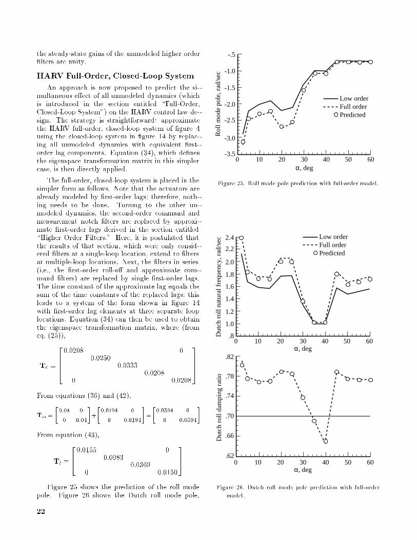
HARV Full-Order, Closed-Loop System
An approach is now proposed to predict the si-multaneous e�ect of all unmodeled dynamics (whichis introduced in the section entitled \Full-Order,Closed-Loop System") on the HARV control law de-sign. The strategy is straightforward: approximatethe HARV full-order, closed-loop system of �gure 4using the closed-loop system in �gure 14 by replac-ing all unmodeled dynamics with equivalent �rst-order lag components. Equation (34), which de�nesthe eigenspace transformation matrix in this simplercase, is then directly applied.
The full-order, closed-loop system is placed in thesimpler form as follows. Note that the actuators arealready modeled by �rst-order lags; therefore, noth-ing needs to be done. Turning to the other un-modeled dynamics, the second-order command andmeasurement notch �lters are replaced by approxi-mate �rst-order lags derived in the section entitled\Higher Order Filters." Here, it is postulated thatthe results of that section, which were only consid-ered �lters at a single-loop location, extend to �ltersat multiple-loop locations. Next, the �lters in series(i.e., the �rst-order roll-o� and approximate com-mand �lters) are replaced by single �rst-order lags.The time constant of the approximate lag equals thesum of the time constants of the replaced lags; thisleads to a system of the form shown in �gure 14with �rst-order lag elements at three separate looplocations. Equation (34) can then be used to obtainthe eigenspace transformation matrix, where (fromeq. (25)),
Te =
266640:0208 0
0:02500:0333
0:02080 0:0208
37775
From equations (36) and (42),
Tm =
�0:04 0
0 0:04
�+
�0:0194 0
0 0:0194
�=
�0:0594 0
0 0:0594
�
From equation (43),
Tl=
2640:0155 0
0:00830:0369
0 0:0150
375
Figure 25 shows the prediction of the roll modepole. Figure 26 shows the Dutch roll mode pole.
-.5
-1.0
-1.5
-2.0
-2.5
-3.0
-3.5100 20 30
α, deg
Rol
l mod
e po
le, r
ad/s
ec
40 50 60
Low orderFull orderPredicted
Figure 25. Roll mode pole prediction with full-order model.
2.4
2.0
2.2
1.8
1.6
1.2
1.0
1.4
.80 10 20 30
α, deg
Dut
ch r
oll n
atur
al f
requ
ency
, rad
/sec
40 50 60
.82
.78
.74
.70
.66
0.62
10 20 30α, deg
Dut
ch r
oll d
ampi
ng r
atio
40 50 60
Low orderFull orderPredicted
Figure 26. Dutch roll mode pole prediction with full-order
model.
22

6
5Low orderFull orderPredicted
4
3
2
1
0 10 20 30α, deg
40 50 60
.020
.016
.012
.008
.004
0 10 20 30α, deg
40 50 60
β-to
-p r
atio
in
roll
mod
e ei
genv
ecto
r, s
ecφ-
to-β
rat
io in
D
utch
rol
l eig
enve
ctor
Figure 27. Eigenvector prediction with full-order model.
Figure 27 contains the eigenvector element ratio pre-diction. As before, the eigenvalues and the eigen-vectors of E�1ALO predict the rigid-body eigenspaceof the 25th-order, closed-loop system.
Conclusions and Recommendations
The approach presented in this report allows thecontrol law designer to predict to what extent un-modeled dynamics a�ect the closed-loop, rigid-bodyeigenspace. Such insight is important when decid-ing which dynamics will be included in the modelused to design the controller. A single-input, single-output example was used to illustrate and predict thee�ect of unmodeled dynamics on a closed-loop, rigid-body pole. This result was extended to multiple-input, multiple-output dynamics, thus leading tothe concept of an eigenspace transformation ma-trix that relates the desired closed-loop rigid-body
eigenspace to that obtained in the presence of un-modeled dynamics.
The approach was �rst developed for unmodeled�rst-order lag elements at one speci�c loop locationand then extended to multiple-loop locations. Theeigenspace transformation matrix was shown to ac-curately predict the achieved rigid-body eigenspacefor this type of unmodeled dynamics. For higherorder unmodeled �lters with a steady-state gain ofunity, derived approximate �rst-order lag compo-nents were shown to be a suitable replacement inpredicting the achieved rigid-body eigenspace. Theapproximate components were easily found from thestate-space expressions of the unmodeled higher or-der �lters. Also, the aggregate e�ect of many typesof unmodeled dynamics on the achieved rigid-bodyeigenspace was shown to be well predicted.
In conclusion, note that there will always besome errors in the achieved rigid-body eigenspace,whether they are caused by poor mathematical mod-els, o�-design ight conditions, or unmodeled dynam-ics. The goal is to �nd what these errors are anddetermine if they will be acceptable. A method forpredicting how some unmodeled dynamics a�ect therigid-body eigenspace is now available.
Some important areas of future work suggestedby this research include the following:
1. Developing a method to predict the achievedrigid-body dynamics when a signi�cant frequencyseparation does not exist between the rigid-bodyand unmodeled dynamics (i.e., when the convergencecriteria would be violated)
2. Formulating sensitivity relationships that de-termine changes in the achieved rigid-body dynamicscaused by incremental changes in unmodeled equiv-alent �rst-order lag time constants
3. Developing a desired eigenspace adjustmentprocedure to account for the e�ect of unmodeled dy-namics on the �nal full-order, closed-loop eigenspaceusing the eigenspace transformation matrix concept
4. Developing methods to change the designmodel, instead of the desired eigenspace, to accountfor the e�ect of unmodeled dynamics in the controlsystem design process
NASA Langley Research Center
Hampton, VA 23681-0001
January 31, 1994
23

Appendix A
HARV Lateral-Directional Aircraft
Model
This appendix contains the linear models repre-senting the High Alpha Research Vehicle (HARV)lateral-directional rigid-body aircraft dynamics atthe 13 ight conditions used in this study. A fullnonlinear model (ref. 7), written in the AdvancedControl Simulation Language (ACSL), was used togenerate these Jacobians. The form of the linear sys-tem is
_x = Ax+Bu (Low-order dynamics)
z =Mx+Nu (System measurements)
with four states, four measurements, and �ve e�ec-tors. The states are lateral velocity, stability-axis rollrate, stability-axis yaw rate, and bank angle (given inunits of feet per second, radians per second, radiansper second, and radians, respectively). The measure-ments are body-axis roll rate, body-axis yaw rate, lat-eral acceleration, and sideslip rate (given in units ofradians per second, radians per second, g units, andradians per second, respectively). The e�ectors areaileron, rudder, asymmetric stabilator, yaw thrustvectoring, and roll thrust vectoring (all given in unitsof degrees).
Finite di�erencing was used to generate theJacobians. Table A1 contains the perturbation stepsize on states and e�ectors used to generate theJacobians. These Jacobians are listed in table A2.
Table A1. Finite Di�erencing Perturbation Sizes
Perturbation Perturbation
State size E�ector size, deg
�s VT=10 ft/sec �ail 2
ps .08 rad/sec �rud??
rs .08 rad/sec �as??
�s .04 rad �ytv??
�rtv
?y
The open-loop roll and spiral mode poles for each ight condition are shown in �gure A1. Figure A2shows the open-loop Dutch roll frequency and damp-ing. Figure A3 contains plots of the two open-loopeigenvector characteristics used in the numerical ex-amples to quantify modal coupling. Note that the�-to-� ratio is nondimensional.
.5
0
–.5
–1.0
–1.5
–2.0
–2.5
–3.00 10 20 30 40 50 60
α, deg
Mod
e po
le, r
ad/s
ec
Spiral mode Roll mode
Figure A1. Roll and spiral mode poles of open-loop aircraft.
2.5
0 10 20 30 40 50 60α, deg
Dut
ch r
oll m
ode
pole
s
Natural frequency, rad/secDamping ratio
2.0
1.5
1.0
.5
0
–.5
Figure A2. Dutch roll mode pole of open-loop aircraft.
3.5
10 20 30 40 50 60α, deg
Eig
enve
ctor
ele
men
t rat
ios
φ-to-β ratio in Dutch rollβ-to-p ratio in roll mode, sec
3.0
2.5
2.0
.5
0
1.0
1.5
Figure A3. �-to-� in Dutch roll and �-to-p roll mode eigen-
vector element ratios of open-loop aircraft.
24

Table A2. HARV Jacobians
� = 2:5� VT = 837 ft/sec
A =
�0:1855 0:0072 �836:1471 32:1675
�0:0271 �2:7580 0:6086 0:0000
0:0058 0:1084 �0:1614 0:0000
0:0000 1:0000 0:0000 0:0000
B =
�0:0946 0:5304 �0:2000 0:2628 0:0056
0:4398 0:0578 0:4538 �0:0048 0:0181
�0:0209 �0:0419 �0:0171 �0:0317 �0:0015
0:0000 0:0000 0:0000 0:0000 0:0000
M =
0:0000 0:9990 �0:0436 0:0000
0:0000 0:0436 0:9990 0:0000
�0:0030 0:0964 �0:0560 0:0000
�0:0002 0:0000 �0:9993 0:0384
N=
0:0000 0:0000 0:0000 0:0000 0:0000
0:0000 0:0000 0:0000 0:0000 0:0000
�0:0197 �0:0009 �0:0218 �0:0041 �0:0008
�0:0001 0:0006 �0:0002 0:0003 0:0000
� = 5� VT = 598 ft/sec
A =
�0:1305 0:1512 �597:5921 32:1675
�0:0187 �1:5272 0:6757 0:0000
0:0050 0:1152 �0:1529 0:0000
0:0000 1:0000 0:0000 0:0000
B =
�0:0551 0:2975 �0:1025 0:2461 0:0024
0:2746 0:0314 0:2224 �0:0059 0:0176
�0:0283 �0:0242 �0:0161 �0:0294 �0:0019
0:0000 0:0000 0:0000 0:0000 0:0000
M =
0:0000 0:9962 �0:0872 0:0000
0:0000 0:0872 0:9962 0:0000
�0:0021 0:0535 �0:0462 0:0000
�0:0002 0:0003 �0:9992 0:0538
25

Table A2. Continued
N=
0:0000 0:0000 0:0000 0:0000 0:0000
0:0000 0:0000 0:0000 0:0000 0:0000
�0:0134 �0:0002 �0:0100 �0:0038 �0:0007
�0:0001 0:0005 �0:0002 0:0004 0:0000
� = 10� VT = 421 ft/sec
A =
�0:0955 0:1610 �420:2861 32:1674
�0:0194 �0:8687 0:6852 0:0000
0:0062 0:1333 �0:1871 0:0000
0:0000 1:0000 0:0000 0:0000
B =
�0:0286 0:1409 �0:0358 0:2500 0:0006
0:1350 0:0146 0:1010 �0:0085 0:0177
�0:0261 �0:0130 �0:0161 �0:0291 �0:0032
0:0000 0:0000 0:0000 0:0000 0:0000
M =
0:0000 0:9848 �0:1736 0:0000
0:0000 0:1736 0:9848 0:0000
�0:0012 0:0295 �0:0392 0:0000
�0:0002 0:0004 �0:9991 0:0765
N=
0:0000 0:0000 0:0000 0:0000 0:0000
0:0000 0:0000 0:0000 0:0000 0:0000
�0:0068 �0:0002 �0:0042 �0:0038 �0:0007
�0:0001 0:0003 �0:0001 0:0006 0:0000
� = 15� VT = 361 ft/sec
A =
�0:0702 0:1331 �360:9948 32:1679
�0:0185 �0:5227 0:6580 0:0000
0:0069 0:1218 �0:2358 0:0000
0:0000 1:0000 0:0000 0:0000
B =
�0:0198 0:0873 �0:0149 0:2497 �0:0013
0:0817 0:0078 0:0618 �0:0105 0:0174
�0:0236 �0:0089 �0:0160 �0:0282 �0:0045
0:0000 0:0000 0:0000 0:0000 0:0000
26
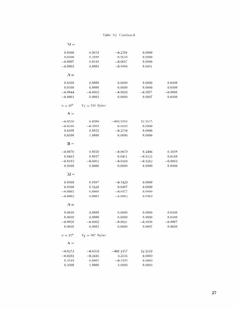
Table A2. Continued
M =
0:0000 0:9659 �0:2588 0:0000
0:0000 0:2588 0:9659 0:0000
�0:0007 0:0169 �0:0407 0:0000
�0:0002 0:0004 �0:9994 0:0891
N=
0:0000 0:0000 0:0000 0:0000 0:0000
0:0000 0:0000 0:0000 0:0000 0:0000
�0:0044 �0:0002 �0:0026 �0:0037 �0:0006
�0:0001 0:0002 0:0000 0:0007 0:0000
� = 20� VT = 334 ft/sec
A =
�0:0558 0:0399 �333:9384 32:1655
�0:0236 �0:2994 0:6024 0:0000
0:0095 0:0932 �0:2796 0:0000
0:0000 1:0000 0:0000 0:0000
B =
�0:0076 0:0559 �0:0079 0:2406 0:0038
0:0463 0:0037 0:0451 �0:0121 0:0160
�0:0183 �0:0061 �0:0168 �0:0262 �0:0063
0:0000 0:0000 0:0000 0:0000 0:0000
M =
0:0000 0:9397 �0:3420 0:0000
0:0000 0:3420 0:9397 0:0000
�0:0005 0:0069 �0:0477 0:0000
�0:0002 0:0001 �1:0002 0:0963
N=
0:0000 0:0000 0:0000 0:0000 0:0000
0:0000 0:0000 0:0000 0:0000 0:0000
�0:0026 �0:0002 �0:0021 �0:0036 �0:0007
0:0000 0:0002 0:0000 0:0007 0:0000
� = 25� VT = 307 ft/sec
A =
�0:0472 �0:0569 �308:1857 32:1649
�0:0191 �0:2336 0:5856 0:0000
0:0103 0:0901 �0:3405 0:0000
0:0000 1:0000 0:0000 0:0000
27
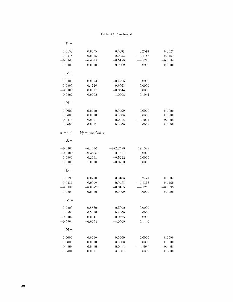
Table A2. Continued
B =
0:0108 0:0375 0:0061 0:2548 0:0027
0:0315 0:0005 0:0355 �0:0158 0:0169
�0:0162 �0:0035 �0:0180 �0:0260 �0:0084
0:0000 0:0000 0:0000 0:0000 0:0000
M =
0:0000 0:9063 �0:4226 0:0000
0:0000 0:4226 0:9063 0:0000
�0:0002 0:0007 �0:0544 0:0000
�0:0002 �0:0002 �1:0006 0:1044
N=
0:0000 0:0000 0:0000 0:0000 0:0000
0:0000 0:0000 0:0000 0:0000 0:0000
�0:0015 �0:0001 �0:0018 �0:0037 �0:0008
0:0000 0:0001 0:0000 0:0008 0:0000
� = 30� VT = 282 ft/sec
A =
�0:0403 �0:1336 �282:2590 32:1549
�0:0099 �0:3858 0:7811 0:0000
0:0060 0:2001 �0:5262 0:0000
0:0000 1:0000 �0:0280 0:0000
B =
0:0195 0:0270 0:0183 0:2471 0:0007
0:0211 �0:0006 0:0288 �0:0167 0:0166
�0:0137 �0:0022 �0:0185 �0:0243 �0:0099
0:0000 0:0000 0:0000 0:0000 0:0000
M =
0:0000 0:8660 �0:5000 0:0000
0:0000 0:5000 0:8660 0:0000
�0:0007 0:0041 �0:0675 0:0000
�0:0001 �0:0005 �1:0009 0:1140
N=
0:0000 0:0000 0:0000 0:0000 0:0000
0:0000 0:0000 0:0000 0:0000 0:0000
�0:0008 0:0000 �0:0013 �0:0036 �0:0008
0:0001 0:0001 0:0001 0:0009 0:0000
28

Table A2. Continued
� = 35� VT = 268 ft/sec
A =
�0:0423 �0:2074 �267:5458 31:9377
�0:0027 �0:3022 0:8106 0:0000
0:0019 0:1766 �0:6487 0:0000
0:0000 1:0000 �0:1202 0:0000
B =
0:0246 0:0214 0:0250 0:2432 0:0007
0:0155 �0:0011 0:0246 �0:0183 0:0155
�0:0124 �0:0015 �0:0196 �0:0226 �0:0112
0:0000 0:0000 0:0000 0:0000 0:0000
M =
0:0000 0:8192 �0:5736 0:0000
0:0000 0:5736 0:8192 0:0000
�0:0012 �0:0048 �0:0715 0:0000
�0:0002 �0:0008 �1:0010 0:1195
N=
0:0000 0:0000 0:0000 0:0000 0:0000
0:0000 0:0000 0:0000 0:0000 0:0000
�0:0005 �0:0001 �0:0011 �0:0036 �0:0008
0:0001 0:0001 0:0001 0:0009 0:0000
� = 40� VT = 261 ft/sec
A =
�0:0435 �0:2705 �261:6818 31:4210
0:0003 �0:3069 0:6522 0:0000
�0:0018 0:2127 �0:6251 0:0000
0:0000 1:0000 �0:2193 0:0000
B =
0:0257 0:0181 0:0277 0:2401 0:0007
0:0125 �0:0018 0:0210 �0:0198 0:0143
�0:0123 �0:0008 �0:0208 �0:0208 �0:0124
0:0000 0:0000 0:0000 0:0000 0:0000
M =
0:0000 0:7660 �0:6428 0:0000
0:0000 0:6428 0:7660 0:0000
�0:0018 �0:0081 �0:0628 0:0000
�0:0002 �0:0010 �1:0008 0:1202
29

Table A2. Continued
N=
0:0000 0:0000 0:0000 0:0000 0:0000
0:0000 0:0000 0:0000 0:0000 0:0000
�0:0004 �0:0001 �0:0011 �0:0036 �0:0008
0:0001 0:0001 0:0001 0:0009 0:0000
� = 45� VT = 262 ft/sec
A =
�0:0383 �0:2061 �261:3775 30:5801
�0:0105 0:1843 0:0830 0:0000
0:0088 �0:2481 �0:1543 0:0000
0:0000 1:0000 �0:3264 0:0000
B =
0:0079 0:0162 0:0265 0:2349 0:0007
0:0109 �0:0030 0:0247 �0:0211 0:0131
�0:0129 0:0004 �0:0269 �0:0189 �0:0135
0:0000 0:0000 0:0000 0:0000 0:0000
M =
0:0000 0:7071 �0:7071 0:0000
0:0000 0:7071 0:7071 0:0000
�0:0012 �0:0350 �0:0210 0:0000
�0:0001 �0:0008 �0:9994 0:1169
N=
0:0000 0:0000 0:0000 0:0000 0:0000
0:0000 0:0000 0:0000 0:0000 0:0000
�0:0009 �0:0001 �0:0011 �0:0036 �0:0008
0:0000 0:0001 0:0001 0:0009 0:0000
� = 50� VT = 262 ft/sec
A =
�0:0333 0:0412 �261:3253 29:4804
�0:0077 �0:0330 0:2272 0:0000
0:0084 �0:0162 �0:3423 0:0000
0:0000 1:0000 �0:4366 0:0000
B =
�0:0118 0:0147 0:0367 0:2294 0:0007
0:0087 �0:0035 0:0240 �0:0222 0:0117
�0:0129 0:0014 �0:0290 �0:0170 �0:0144
0:0000 0:0000 0:0000 0:0000 0:0000
30

Table A2. Continued
M =
0:0000 0:6428 �0:7660 0:0000
0:0000 0:7660 0:6428 0:0000
�0:0008 �0:0122 �0:0208 0:0000
�0:0001 0:0002 �0:9985 0:1126
N=
0:0000 0:0000 0:0000 0:0000 0:0000
0:0000 0:0000 0:0000 0:0000 0:0000
�0:0016 �0:0001 �0:0003 �0:0036 �0:0008
0:0000 0:0001 0:0001 0:0009 0:0000
� = 55� VT = 266 ft/sec
A =
�0:0380 0:1644 �265:4073 28:4186
�0:0065 �0:0508 0:2138 0:0000
0:0087 0:0197 �0:3784 0:0000
0:0000 1:0000 �0:5303 0:0000
B =
�0:0145 0:0143 0:0719 0:2260 0:0007
0:0064 �0:0030 0:0309 �0:0229 0:0103
�0:0124 0:0011 �0:0380 �0:0150 �0:0152
0:0000 0:0000 0:0000 0:0000 0:0000
M =
0:0000 0:5736 �0:8192 0:0000
0:0000 0:8192 0:5736 0:0000
�0:0009 �0:0050 �0:0240 0:0000
�0:0001 0:0006 �0:9990 0:1070
N=
0:0000 0:0000 0:0000 0:0000 0:0000
0:0000 0:0000 0:0000 0:0000 0:0000
�0:0017 �0:0002 0:0018 �0:0036 �0:0008
�0:0001 0:0001 0:0003 0:0009 0:0000
� = 60� VT = 276 ft/sec
A =
�0:0472 0:1523 �275:5784 26:6075
�0:0058 �0:0638 0:2364 0:0000
0:0089 0:0320 �0:3957 0:0000
0:0000 1:0000 �0:6794 0:0000
31

Table A2. Concluded
B =
�0:0156 0:0144 0:1012 0:2251 �0:0071
0:0051 �0:0022 0:0227 �0:0236 0:0107
�0:0131 �0:0001 �0:0296 �0:0128 �0:0144
0:0000 0:0000 0:0000 0:0000 0:0000
M =
0:0000 0:5000 �0:8660 0:0000
0:0000 0:8660 0:5000 0:0000
�0:0013 �0:0083 �0:0097 0:0000
�0:0002 0:0006 �0:9995 0:0965
N=
0:0000 0:0000 0:0000 0:0000 0:0000
0:0000 0:0000 0:0000 0:0000 0:0000
�0:0018 �0:0003 0:0037 �0:0034 �0:0001
�0:0001 0:0001 0:0004 0:0008 0:0000
32

Appendix B
Baseline HARV Flight Control System
Gains
This appendix contains the linear feed-forwardand measurement feedback gains for the 13 ightconditions considered. There are two controls and�ve e�ectors. As previously stated, the e�ectors areaileron, rudder, asymmetric stabilator, yaw thrustvectoring, and roll thrust vectoring (which are allmeasured in degrees). The measurements are body-axis roll and yaw rate (which are measured in radiansper second), sensed lateral acceleration (which ismeasured in g units), and sensed sideslip rate (whichis measured in radians per second). The controlsare commanded roll and yaw acceleration (which aremeasured in radians per second squared). The feed-forward and measurement feedback gain matrices arelisted in table B1.
The feed-forward gains are designed such that thetwo controls are mapped into the �ve e�ectors. The
two controls are commanded roll and yaw angularacceleration. The feed-forward gain matrix is aJacobian of a control mapping algorithm (discussedin ref. 6), which is evaluated at the various trimmed ight conditions. For the purposes of this research,the set of feed-forward gain matrices is assumed tobe given. The controls are a sum of pilot input andfeedback (�g. 3),
u = K(uFB + upilot)
The measurement feedback gain matrices map thefour measurements into the two controls such that
uFB = Gz
The baseline gains listed were designed using theCRAFT (control power, robustness, agility, and ying-qualities trade-o�s) procedure of reference 2.These gains are designed to be scheduled with angleof attack.
33
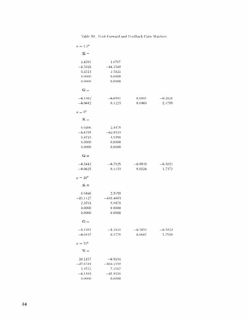
Table B1. Feed-Forward and Feedback Gain Matrices
� = 2:5�
K=
2:4595 1:6767
�1:5926 �34:1549
0:3513 2:5021
0:0000 0:0000
0:0000 0:0000
G=
�0:1062 �0:6541 0:0441 �0:2824
�0:0642 0:1223 0:0460 2:1799
� = 5�
K=
4:0206 2:4478
�5:6765 �62:0159
0:8725 4:9350
0:0000 0:0000
0:0000 0:0000
G=
�0:5442 �0:7925 �0:0019 �0:3825
�0:0625 0:1133 0:0524 1:7372
� = 10�
K=
6:9486 2:5159
�21:1127 �116:4603
2:3793 8:9879
0:0000 0:0000
0:0000 0:0000
G=
�1:1081 �1:2024 �0:1014 �0:1852
�0:0437 0:1778 0:0607 1:7539
� = 15�
K=
10:1457 �0:9134
�27:6594 �103:2218
3:4755 7:2567
�6:1403 �21:9256
0:0000 0:0000
34

Table B1. Continued
G =
�1:2663 �1:1728 �0:0005 �0:6436
0:0228 0:2459 0:0600 1:5931
� = 20�
K =
14:2474 �5:3125
�33:5753 �90:8832
5:0302 3:8308
�11:3867 �30:2217
0:0000 0:0000
G =
�1:4859 �2:0383 �0:6063 �1:2320
0:0681 0:3996 0:2004 1:9451
� = 25�
K =
14:1097 �14:4480
�41:1839 �84:1229
4:7607 �1:7777
�13:5142 �28:1494
0:0000 0:0000
G =
�1:5959 �1:9635 0:3622 �1:1257
0:0885 0:4970 0:0183 2:1152
� = 30�
K =
13:2511 �23:2949
�47:7514 �75:2633
3:9250 �7:5768
�15:1551 �25:5799
0:0000 0:0000
G =
�0:4186 �2:2548 0:1121 �1:2376
�0:2107 0:7058 �0:0254 1:6765
35
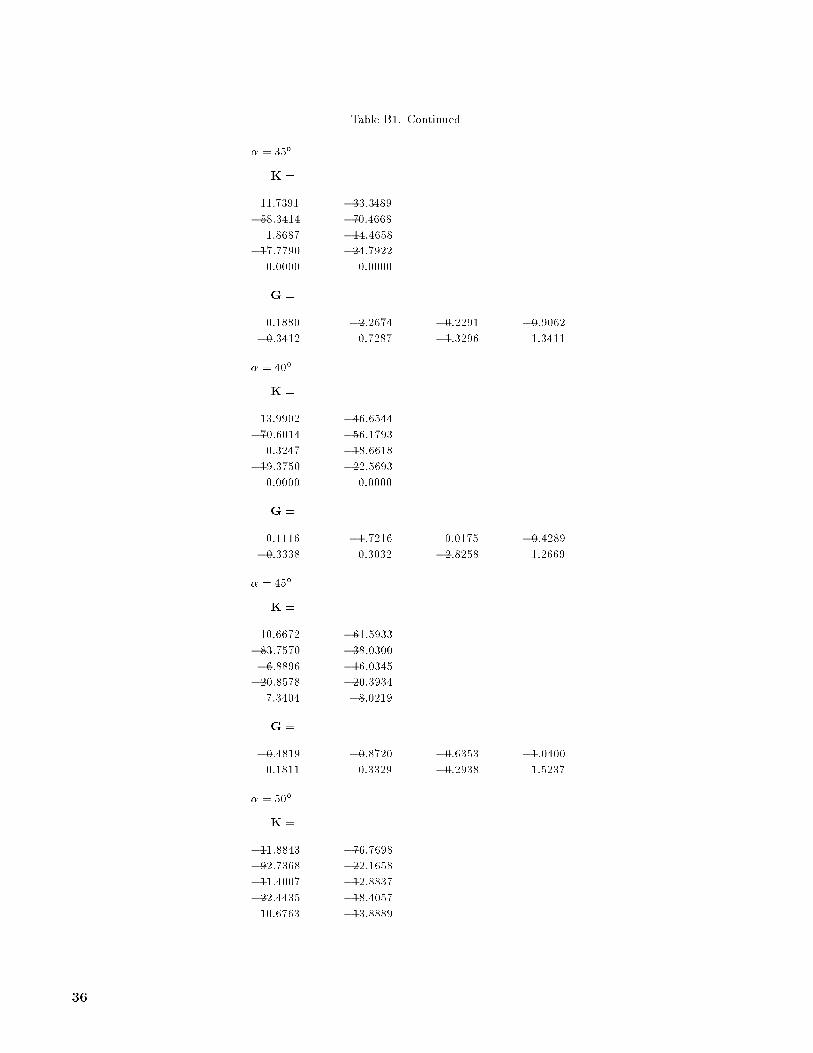
Table B1. Continued
� = 35�
K =
11:7391 �33:3489
�58:3414 �70:4668
1:8687 �14:4658
�17:7790 �24:7922
0:0000 0:0000
G =
0:1880 �2:2674 �0:2291 �0:9062
�0:3412 0:7287 �1:3296 1:3411
� = 40�
K =
13:9902 �46:6544
�70:6014 �56:1793
0:3247 �18:6618
�19:3750 �22:5693
0:0000 0:0000
G =
0:1116 �1:7216 0:0175 �0:4289
�0:3338 0:3032 �2:8258 1:2669
� = 45�
K =
10:6672 �61:5933
�83:7570 �38:0300
�6:8896 �16:0345
�20:8578 �20:3934
7:3404 �8:0219
G =
�0:4819 �0:8720 �0:6353 �1:0400
0:1811 0:3329 �0:2938 1:5237
� = 50�
K =
�11:8843 �76:7698
�92:7368 �22:1658
�11:4007 �12:8837
�22:4435 �18:4057
10:6763 �13:8889
36

Table B1. Concluded
G =
�0:1495 �1:0156 �0:2759 �0:9231
�0:0301 0:4716 0:2016 1:3646
� = 55�
K =
�29:1475 �83:0683
�89:7036 �0:6993
�2:1824 �1:6032
�25:2961 �17:2914
11:6376 �18:5082
G =
�0:1753 �0:8326 �0:0765 �0:7941
�0:0716 0:4357 0:1557 1:5059
� = 60�
K =
�37:1976 �83:9399
�66:6277 0:3374
0:0000 0:0000
�27:7290 �15:5958
13:9318 �27:0141
G =
�0:4204 �0:5479 �0:3657 �0:1400
0:0113 0:3407 0:2077 1:3010
37

References
1. Pahle, Joseph W.; Powers, Bruce; Regenie, Victoria;
Chacon, Vince; DeGroote, Steve; and Murnyak, Steven:
Research Flight-Control System Development for the F-18
High Alpha Research Vehicle. NASA TM-104232,
1991.
2. Murphy, Patrick C.; and Davidson, John B.: Control
Design for Future Agile Fighters. AIAA-91-2882, Aug.
1991.
3. Andry, A. N., Jr.; Shapiro, E. Y.; and Chung, J. C.:
Eigenstructure Assignment for Linear Systems. IEEE
Trans. Aerosp. & Electron. Syst., vol. AES-19, no. 5,
Sept. 1983, pp. 711{729.
4. Davidson, J. B.; and Schmidt, D. K.: Flight Control Syn-
thesis for Flexible Aircraft Using EigenspaceAssignment.
NASA CR-178164, 1986.
5. McRuer,Duane; Ashkenas, Irving; andGraham,Dunstan:
Aircraft Dynamics and Automatic Control. Princeton
Univ. Press, 1973.
6. Lallman, Frederick J.: Relative Control E�ectiveness
Technique With Application to Airplane Control Coordi-
nation. NASA TP-2416, 1985.
7. Buttrill, Carey S.; Arbuckle, P. Douglas; and Ho�er,
Keith D.: Simulation Model of a Twin-Tail, High Per-
formance Airplane. NASA TM-107601, 1992.
8. Burden, Richard L.; and Faires, J. Douglas: Numerical
Analysis, 4th ed. PWS-KENTPubl. Co., 1989.
38
References
1. Pahle, Joseph W.; Powers, Bruce; Regenie, Vic-
toria; Chacon, Vince; DeGroote, Steve; and
Murnyak, Steven: Research Flight-Control Sys-
tem Development for the F-18 High Alpha Re-
search Vehicle. NASA TM-104232, 1991.
2. Murphy, Patrick C.; and Davidson, John B.: Con-
trol Design for Future Agile Fighters. AIAA 91-
2882, Aug. 1991.
3. Andry, A. N., Jr.; Shapiro, E. Y.; and Chung,
J. C.: Eigenstructure Assignment for Linear Sys-
tems. IEEE Trans. Aerosp. & Electron. Syst.,
vol. AES-19, no. 5, Sept. 1983, pp. 711{729.
4. Davidson, J. B.; and Schmidt, D. K.: Flight Con-
trol Synthesis for Flexible Aircraft Using Eigenspace
Assignment. NASA CR-178164, 1986.
5. McRuer, Duane; Ashkenas, Irving; and Graham,
Dunstan: Aircraft Dynamics and Automatic Con-
trol. Princeton Univ. Press, 1973.
6. Lallman, Frederick J.: Relative Control E�ec-
tiveness Technique With Application to Airplane
Control Coordination. NASA TP-2416, 1985.
7. Buttrill, Carey S.; Arbuckle, P. Douglas; and
Ho�er, Keith D.: Simulation Model of a Twin-
Tail, High Performance Airplane. NASA TM-
107601, 1992.
8. Burden, Richard L.; and Faires, J. Douglas: Nu-
merical Analysis, 4th ed. PWS-KENT Publ. Co.,
c.1989.
1

REPORT DOCUMENTATION PAGEForm Approved
OMB No. 0704-0188
Public reporting burden for this collection of information is estimated to average 1 hour per response, including the time for reviewing instructions, searching existing data sources,gathering and maintaining the data needed, and completing and reviewing the collection of information. Send comments regarding this burden estimate or any other aspect of thiscollection of information, including suggestions for reducing this burden, toWashington Headquarters Services, Directorate for Information Operations and Reports, 1215 Je�ersonDavis Highway, Suite 1204, Arlington, VA 22202-4302, and to the O�ce of Management and Budget, Paperwork Reduction Project (0704-0188), Washington, DC 20503.
1. AGENCY USE ONLY(Leave blank) 2. REPORT DATE 3. REPORT TYPE AND DATES COVERED
June 1994 Technical Memorandum
4. TITLE AND SUBTITLE
Predicting the E�ects of Unmodeled Dynamics on an AircraftFlight Control System Design Using Eigenspace Assignment
6. AUTHOR(S)
Eric N. Johnson, John B. Davidson, and Patrick C. Murphy
7. PERFORMING ORGANIZATION NAME(S) AND ADDRESS(ES)
NASA Langley Research CenterHampton, VA 23681-0001
9. SPONSORING/MONITORING AGENCY NAME(S) AND ADDRESS(ES)
National Aeronautics and Space AdministrationWashington, DC 20546-0001
5. FUNDING NUMBERS
WU 505-64-52-01
8. PERFORMING ORGANIZATION
REPORT NUMBER
L-17333
10. SPONSORING/MONITORING
AGENCY REPORT NUMBER
NASA TM-4548
11. SUPPLEMENTARY NOTES
Johnson: The George Washington University, Washington, D.C.; Davidson and Murphy: Langley ResearchCenter, Hampton, VA.
12a. DISTRIBUTION/AVAILABILITY STATEMENT 12b. DISTRIBUTION CODE
Unclassi�ed{Unlimited
Subject Category 08
13. ABSTRACT (Maximum 200 words)
When using eigenspace assignment to design an aircraft ight control system, one must �rst develop a modelof the plant. Certain questions arise when creating this model as to which dynamics of the plant need to beincluded in the model and which dynamics can be left out or approximated. The answers to these questions areimportant because a poor choice can lead to closed-loop dynamics that are unpredicted by the design model.To alleviate this problem, a method has been developed for predicting the e�ect of not including certaindynamics in the design model on the �nal closed-loop eigenspace. This development provides insight as towhich characteristics of unmodeled dynamics will ultimately a�ect the closed-loop rigid-body dynamics. Whatresults from this insight is a guide for eigenstructure control law designers to aid them in determining whichdynamics need or do not need to be included and a new way to include these dynamics in the ight controlsystem design model to achieve a required accuracy in the closed-loop rigid-body dynamics. The method isillustrated for a lateral-directional ight control system design using eigenspace assignment for the NASA HighAlpha Research Vehicle (HARV).
14. SUBJECT TERMS 15. NUMBER OF PAGES
Eigenspace assignment; Unmodeled dynamics; High Alpha Research Vehicle;Lateral-directional aircraft control system
39
16. PRICE CODE
A0317. SECURITY CLASSIFICATION 18. SECURITY CLASSIFICATION 19. SECURITY CLASSIFICATION 20. LIMITATION
OF REPORT OF THIS PAGE OF ABSTRACT OF ABSTRACT
Unclassi�ed Unclassi�ed
NSN 7540-01-280-5500 Standard Form 298(Rev. 2-89)Prescribed by ANSI Std. Z39-18298-102