Predicting Phonon Properties from

Equilibrium Molecular Dynamics Simulations

Alan J. H. McGaughey∗ and Jason M. Larkin

Department of Mechanical Engineering, Carnegie Mellon University

5000 Forbes Ave., Pittsburgh PA 15213

∗ Address all correspondences to Alan J. H. McGaughey, mcgaughey@cmu

Abstract

The objective of this chapter is to describe how equilibrium molecular dynamics simula-

tions (with the help of harmonic lattice dynamics calculations) can be used to predict phonon

properties and thermal conductivity using normal mode decomposition. The molecular dy-

namics and lattice dynamics methods are reviewed and the normal mode decomposition

technique is described in detail. The application of normal mode decomposition is demon-

strated through case studies on crystalline, alloy, and amorphous Lennard-Jones phases.

Notable works that used normal mode decomposition are presented and the future of molec-

ular dynamics simulations in phonon transport modeling is discussed.

Keywords: normal mode decomposition, lattice dynamics calculations, phonon lifetime,

anharmonicity, virtual crystal approximation, vibrational modes in disordered systems

1

Nomenclature

a lattice constant

c alloy concentration

cv volumetric specific heat

C constant

D dynamical matrix

e normal mode polarization vector

E total energy (= K + U)

kB Boltzmann constant, 1.3806× 10−23 J/K

k, k thermal conductivity

K kinetic energy

L MD simulation cell size

m mass

n number of atoms in unit cell

N number of atoms in simulation cell

No number of unit cells in each direction of a cubic simulation cell

q” heat flux

q normal mode coordinate

r particle position

S, S heat current

t time

T temperature

2

u, u particle displacement from equilibrium

U potential energy

vg, vg group velocity

V volume

Greek symbols

Γ line width

κκκ, κ wave vector, wave number

Λ mean free path

ν polarization branch

τ lifetime

ΦΦΦ force constant matrix

ω angular frequency

Subscripts

a anharmonic

b summation index, particle label

i summation index, particle label

j summation index, particle label

l summation index, unit cell label

o equilibrium

α, β, γ x, y, or z direction

3

Superscripts

* complex conjugate

† transpose complex conjugate

Abbreviations

BTE Boltzmann transport equation

DFT density functional theory

HCACFheat current autocorrelation function

IR Ioffe-Regel

LJ Lennard-Jones

MD molecular dynamics

4

1 Introduction

1.1 Motivation: Thermal Conductivity Prediction

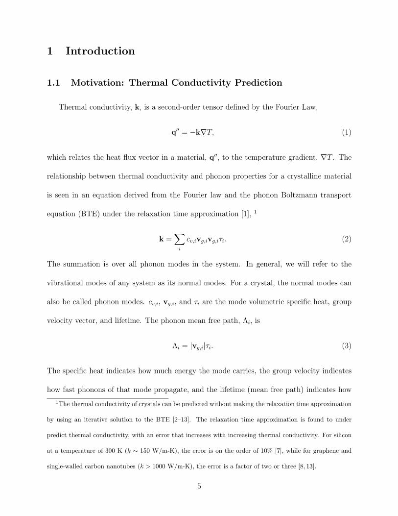
Thermal conductivity, k, is a second-order tensor defined by the Fourier Law,

q′′ = −k∇T, (1)

which relates the heat flux vector in a material, q′′, to the temperature gradient, ∇T . The

relationship between thermal conductivity and phonon properties for a crystalline material

is seen in an equation derived from the Fourier law and the phonon Boltzmann transport

equation (BTE) under the relaxation time approximation [1], 1

k =∑i

cv,ivg,ivg,iτi. (2)

The summation is over all phonon modes in the system. In general, we will refer to the

vibrational modes of any system as its normal modes. For a crystal, the normal modes can

also be called phonon modes. cv,i, vg,i, and τi are the mode volumetric specific heat, group

velocity vector, and lifetime. The phonon mean free path, Λi, is

Λi = |vg,i|τi. (3)

The specific heat indicates how much energy the mode carries, the group velocity indicates

how fast phonons of that mode propagate, and the lifetime (mean free path) indicates how

1The thermal conductivity of crystals can be predicted without making the relaxation time approximation

by using an iterative solution to the BTE [2–13]. The relaxation time approximation is found to under

predict thermal conductivity, with an error that increases with increasing thermal conductivity. For silicon

at a temperature of 300 K (k ∼ 150 W/m-K), the error is on the order of 10% [7], while for graphene and

single-walled carbon nanotubes (k > 1000 W/m-K), the error is a factor of two or three [8, 13].

5

long (far) phonons of that mode travel on average before scattering.

The phonon properties required to predict bulk thermal conductivity can be measured

using neutron, Brillouin, or Raman scattering [14–16]. Such experiments, however, require

resources that are not widely available. Furthermore, not enough phonon modes can be re-

solved to accurately predict thermal conductivity. Recent experimental attention has turned

to using laser-based techniques [17–22], which can resolve how different mean free paths

contribute to the total thermal conductivity (i.e, the thermal conductivity accumulation

function [23]), but cannot provide the properties of individual phonon modes. Theoretical

work is thus of critical importance.

1.2 Theoretical Approaches for Predicting Phonon Properties

Techniques at different levels of sophistication exist for predicting phonon properties

and thermal conductivity (see Table 1). Work in the 1950s, 1960s, and 1970s, notably by

Callaway, Klemens, Holland, and Slack (see e.g., Refs. [24–27]) derived and/or postulated

analytical models for the phonon dispersion and lifetimes (typically based on low-frequency

limits) to be used in a solution of the BTE for predicting thermal conductivity. By fitting the

BTE solution to experimental bulk thermal conductivity data, expressions for the lifetimes

are obtained. While good fits to the experimental data can be found, this agreement may be

due to the numerous fitting parameters and not due to the correctness of the phonon lifetime

models [28]. Atomistic techniques, which can predict the properties of individual phonon

modes without any assumptions about the dispersion or scattering, are thus required.

Given a framework for calculating the force constants between atoms [29–31], it is

6

Callaway/Holland Anharmonic LatticeDynamics

Molecular Dynamics

Description Fit lifetime models toexperimental k data

Perturbation to nor-mal modes from har-monic lattice dynam-ics calculations

Explicit solution tothe Newtonian lawsof motion and projec-tion onto harmonicnormal modes

Input Dispersion and life-time models, experi-mental k data

Force constants(from DFT or poten-tials)

Forces(from potentials)

Anharmonicity Full Third-order FullStatistics Bose-Einstein or

BoltzmannBose-Einstein orBoltzmann

Boltzmann

Temperature All Low HighDisorder As additional

perturbationAs additionalperturbation

Can be naturally in-cluded

Comments Challenging to applyto non-isotropic sys-tems.Requires fitting pa-rameters.

Partial fourth-ordertheory for predictingfrequency shiftsavailable.Calculation scaleswith the fourthpower of the numberof atoms in the unitcell.

Requires a prioriharmonic lattice dy-namics calculations.Can also predictk from top-downtechniques.

Table 1: Comparison of theoretical techniques for predicting phonon properties and thermalconductivity.

7

straightforward to use harmonic lattice dynamics calculations to predict phonon frequen-

cies, and from these, specific heats, dispersion curves, density of states, and group velocities

(see Section 3) [32–35]. To predict phonon lifetimes in the lattice dynamics framework, an-

harmonic calculations are required, which are theoretically complicated and computational

demanding (e.g., they scale with the fourth power of the number of atoms in the unit cell)

[14, 32, 36, 37]. The anharmonic lattice dynamics approach, which allows for the natural

inclusion of Bose-Einstein statistics, is discussed in Chapter [Esfarjani].

When density functional theory (DFT) calculations are used to obtain the force constants

for lattice dynamics calculations, good agreement is found with experimental thermal conduc-

tivity measurements for a range of materials [7, 9, 30, 38–45]. There are limitations, however,

to this approach. First, the existing theoretical framework for predicting phonon lifetimes

only includes three-phonon processes (i.e., cubic force constants are required). Higher-order

phonon processes are not included and will become more important as temperature is in-

creased [37]. For this reason, anharmonic lattice dynamics is a low-temperature method.2

Second, due to their computational demands, DFT calculations are only realistic for small

systems (typically less than 100 atoms). As such, disruptions to periodicity (e.g., point de-

fects) must be included as a perturbation, after the intrinsic properties have been calculated.

The limitation on system size also makes it challenging to model amorphous systems.

Given the outputs of harmonic lattice dynamics calculations, molecular dynamics (MD)

simulations can be used to predict phonon lifetimes using normal mode decomposition (see

Section 4) [36, 37, 46, 47], which is the focus of this chapter. While MD simulations can be

2By low temperature, we mean temperatures below the Debye temperature. By high temperature, we

mean temperature around and above the Debye temperature.

8

driven using forces calculated from DFT, these calculations are expensive and prohibit sim-

ulation of large enough systems for long enough times to properly model phonon transport.

As such, interatomic potentials are typically used to compute the required forces.

Molecular dynamics simulation is a classical technique as it uses the Newtonian equations

of motion to describe the atomic dynamics. The vibrational modes in a MD simulation thus

follow Boltzmann statistics, which is the high-temperature limit of Bose-Einstein statistics.

This technique is therefore suitable for comparing to experimental measurements at high

temperatures, providing a complement to the anharmonic lattice dynamics approach. In

contrast to anharmonic lattice dynamics calculations, MD simulations naturally include the

full anharmonicity of the atomic interactions (i.e., all orders of phonon-phonon interactions),

again making them well-suited to high-temperatures.

1.3 Outline

The over-arching theme of this chapter is to describe how to calculate phonon properties

and thermal conductivity from the output of equilibrium MD simulations. The remainder of

the chapter is organized as follows. In Section 2, we describe the MD simulation technique,

with a focus on top-down thermal conductivity prediction. In Section 3, we briefly review

the harmonic lattice dynamics calculations that are required to perform normal mode de-

composition. In Section 4, we present the normal mode decomposition technique, discuss

issues related to its implementation, and perform a case study on Lennard-Jones (LJ) crys-

tal, alloy, and amorphous phases. In Section 5, we review previous work that used normal

mode decomposition and in Section 6, we discuss the role of MD simulation in future phonon

transport modeling.

9

2 Molecular Dynamics Simulation

2.1 Formulation

In a MD simulation, the Newtonian laws of motion are solved to evolve the positions and

velocities of a set of atoms. The required forces between atoms may be obtained from inter-

atomic potentials (e.g., LJ [48], Stillinger-Weber [49], Tersoff [50]) or from DFT calculations.

Density functional theory calculations are many orders of magnitude more computationally

demanding than evaluating interatomic potentials, which can be analytical functions or look-

up tables. As such, DFT calculations cannot yet be used to drive MD simulations that are

large or long enough to access the length and time scales relevant to atomistic thermal

transport. The basic formulation of MD simulation is covered in reference books [51–53].

McGaughey and Kaviany previously reviewed concepts relevant to MD simulation of solids

with a focus on phonons and thermal transport [54]. In this section, we present a brief

overview.

The required inputs to a MD simulation are initial conditions (atomic positions and ve-

locities) and an interatomic potential. Interatomic potentials are available for many metals

and dielectrics (i.e., electrical insulators and semiconductors). Because electrons are not

explicitly considered in a MD simulation, thermal transport in metals cannot be studied.

The majority of available interatomic potentials for dielectrics, where thermal transport is

dominated by phonons, were not fit to phonon or thermal properties. As a result, most

interatomic potentials do a poor job of predicting experimentally measured thermal conduc-

tivities. For example, none of the commonly-used interatomic potentials for silicon success-

fully predict its thermal conductivity over a range of temperatures [6, 55, 56]. Recent work,

10

however, has demonstrated that interatomic potentials fit to either experimental or DFT

phonon data can do a much better job of predicting experimentally measured thermal con-

ductivities [13, 39, 42]. This advancement suggests that MD simulations, which can access

much larger length and time scales than DFT calculations, will continue to be of use to the

phonon transport community.

An integration scheme and time step are required to numerically solve the Newtonian

equations of motion. Atomistic phenomena occur at terahertz frequencies and a time step

on the order of 1 fs is typical. Second-order integration schemes (e.g., velocity Verlet) are

generally sufficient to conserve energy to four or five significant digits. For bulk simulations,

periodic boundary conditions are applied in all directions. For simulating a nanostructure

(e.g., a film or wire), free boundary conditions may be applied in some directions.

There are three main types of MD simulation related to thermal transport: equilibrium,

steady-state, and unsteady. In an equilibrium simulation, there are no spatial or temporal

gradients in local temperature, allowing for averaging over space and time. Equilibrium

simulations are the focus of this chapter. In a steady-state, non-equilibrium simulation,

spatial temperature variations may exist, but the system is steady in time, allowing for time

averaging. Such simulations allow for direct observations of transport and are discussed in

Chapter [Shiomi]. In an unsteady simulation, spatial and temporal temperature variations

may exist, allowing for observation of processes such as the propagation of a phonon wave

packet [57, 58].

The Newtonian equations of motion conserve energy, leading to simulations in the NV E

[i.e., constant mass (number of atoms), volume, and energy] ensemble. For predicting thermal

conductivity or phonon properties, MD simulations should be run in the NV E ensemble

11

because the relevant analysis techniques, which are described in Sections 2.2 and 4.1, rely

on correlations. These correlations can be artificially influenced by modifications to the

natural dynamics of the atoms, particularly in small systems. Simulations run in the NV T

(i.e., constant mass, volume, and thermodynamic temperature) or NPT (i.e., constant mass,

thermodynamic pressure, and thermodynamic temperature) ensembles, where the Newtonian

equations of motion are modified, are helpful for relaxing structures and finding temperature-

and pressure-dependent lattice constants.

The raw outputs of a MD simulation are the time histories of the positions and velocities

of the constituent atoms. This output can be used to calculate forces, potential energy,

kinetic energy, temperature, pressure, mechanical properties, and transport properties.

2.2 Top-down Thermal Conductivity Prediction

There are two commonly-used top-down techniques for predicting thermal conductivity

from MD simulations: the Green-Kubo method [54, 59], which uses equilibrium simulations,

and the direct method [54, 55], which uses steady-state non-equilibrium simulations. These

two methods are compared in Table 2. While so-called “quantum corrections” to thermal

conductivities predicted from classical MD simulations have been proposed, Turney et al.

demonstrate that these corrections are not rigorous and should not be applied [60]. Compar-

ison of MD-predicted thermal conductivities to experimental measurements should therefore

be limited to high temperatures, around and above a material’s Debye temperature. Top-

down techniques are important in the context of this chapter because they can be used to

validate the bottom-up techniques that are our focus.

12

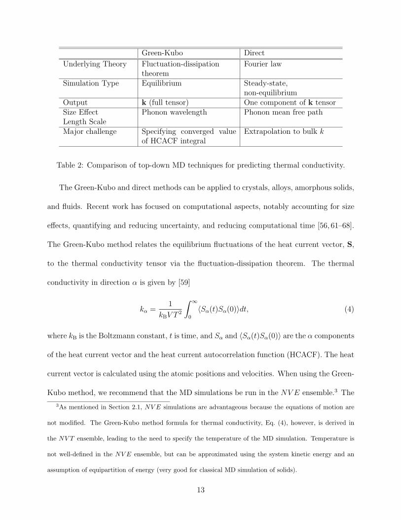
Green-Kubo Direct

Underlying Theory Fluctuation-dissipationtheorem

Fourier law

Simulation Type Equilibrium Steady-state,non-equilibrium

Output k (full tensor) One component of k tensorSize EffectLength Scale

Phonon wavelength Phonon mean free path

Major challenge Specifying converged valueof HCACF integral

Extrapolation to bulk k

Table 2: Comparison of top-down MD techniques for predicting thermal conductivity.

The Green-Kubo and direct methods can be applied to crystals, alloys, amorphous solids,

and fluids. Recent work has focused on computational aspects, notably accounting for size

effects, quantifying and reducing uncertainty, and reducing computational time [56, 61–68].

The Green-Kubo method relates the equilibrium fluctuations of the heat current vector, S,

to the thermal conductivity tensor via the fluctuation-dissipation theorem. The thermal

conductivity in direction α is given by [59]

kα =1

kBV T 2

∫ ∞

0

⟨Sα(t)Sα(0)⟩dt, (4)

where kB is the Boltzmann constant, t is time, and Sα and ⟨Sα(t)Sα(0)⟩ are the α components

of the heat current vector and the heat current autocorrelation function (HCACF). The heat

current vector is calculated using the atomic positions and velocities. When using the Green-

Kubo method, we recommend that the MD simulations be run in the NV E ensemble.3 The

3As mentioned in Section 2.1, NV E simulations are advantageous because the equations of motion are

not modified. The Green-Kubo method formula for thermal conductivity, Eq. (4), however, is derived in

the NV T ensemble, leading to the need to specify the temperature of the MD simulation. Temperature is

not well-defined in the NV E ensemble, but can be approximated using the system kinetic energy and an

assumption of equipartition of energy (very good for classical MD simulation of solids).

13

Green-Kubo method is advantageous for anisotropic materials because it can be used to

predict the full thermal conductivity tensor.

There are two main challenges associated with using the Green-Kubo method to predict

thermal conductivity. First, the system should be large enough to ensure a size-independent

value. Thermal conductivities predicted using the Green-Kubo method show a weak system-

size dependence, typically increasing with increasing system size before converging. As the

resolution of the allowed phonon modes in the Brillouin zone becomes finer, there are two

competing effect that lead to this weak size-dependence: (i) the emergence of long-wavelength

phonon modes that can carry a significant amount of thermal energy, and (ii) an increase

in phonon-phonon scattering due to more modes being available. The system-size effect

in the Green-Kubo method is thus related to the phonon wavelength. Systems sizes of

ten thousand atoms or less are typically sufficient to remove size effects [46, 56, 64, 67] and

are easily handled using current computational resources, particularly given the parallel

capabilities of available MD codes. For a cubic unit cell, a cubic simulation cell is ideal as

the Brillouin zone will be resolved evenly in all directions. For non-cubic unit cells, careful

testing of the effects of the simulation cell size on thermal conductivity are recommended.

The second challenge in the Green-Kubo method is to accurately specify the converged

value of the HCACF. The MD simulation itself should be at least ten times longer than the

longest phonon lifetime in the system. The correlation time used to calculate the HCACF

should be long enough to capture its full decay, which will also be related to the longest

phonon lifetime. As phonon lifetime data may not be available, the MD simulations must

be carefully designed. Of critical importance is to run simulations starting from different

initial conditions (easily obtained by randomizing the velocities, five or ten initial conditions

14

are typically sufficient) and then average the HCACFs from each. The different initial

conditions will allow for an efficient exploration of the phase space and a faster realization of

the true ensemble average. Depending on the material system, averaging over symmetrical

crystallographic directions may also be possible.

Given a properly averaged HCACF, one must then specify the converged value of its

integral. For crystals with small unit cells and low thermal conductivities, the HCACF can

be fit with algebraic expressions (e.g., exponential decays) [56, 69, 70]. For more complicated

unit cells (or disordered systems) and high thermal conductivity materials, however, these fits

are either not possible or not accurate and the integration must be performed numerically [55,

61, 64]. Ideally, one specifies a range of the correlation time where the integral is converged

and then averages over that range. The challenge is that noise in the HCACF, particularly

at long correlation times, contaminates the true response and determining where to evaluate

the integral is difficult. Chen et al. suggest the “first-avalanche” scheme, which is based on

the magnitude of the fluctuations in the HCACF [63]. We recommend use of this robust

scheme.

In the direct method, a heat flow is applied across a simulation cell that is long in one

direction and the resulting temperature gradient is used with the Fourier law, Eq. (1), to

predict the thermal conductivity in that direction. This technique is further described in

Chapter [Shiomi]. The main challenge in applying the direct method is to account for size

effects. As the size of the simulation cell is increased, the thermal conductivity increases

as there is less phonon-boundary scattering. The length scale related to size effects in the

direct method is therefore the phonon mean free path. In cases where thermal conductivity

does not converge as the system size increases, many previous works have used a linear

15

extrapolation method [55], whereby the inverse of thermal conductivity is plotted versus the

inverse of the system size, L, and a line is fit to the data. The vertical coordinate of the

line where 1/L goes to zero is used to obtain the bulk thermal conductivity. One must be

careful when applying this technique however, as Sellan et al. found that the dependence

of 1/k with 1/L may not be linear [64]. Furthermore, for LJ argon, Hu et al. found that,

after reaching a plateau, the thermal conductivity predicted in the direct method can diverge

with increasing system size [71]. They attribute this result to one-dimensional phonon effects

as the resolution of the Brillouin zone becomes very fine in one direction. Howell provides

detailed suggestions on what system sizes to use and how long to run the simulations to

optimize use of the direct method [65, 66].

It is our opinion that the Green-Kubo method is preferred over the direct method because:

(i) smaller systems size can capture the size effects, (ii) the full thermal conductivity tensor

is available, and (iii) the MD simulations are run in the NV E ensemble, with no need to

modify the equations of motion. In some cases, however, the converged value of the HCACF

integral may be too difficult to specify and the direct method is required.

2.3 How to Think About Phonons in an Equilibrium Molecular

Dynamics Simulation

Under the relaxation time approximation, the fundamental quantity associated with

phonon scattering is the mode lifetime – how long, on average, an excess of phonons ex-

ists before the energy is scattered into other modes. The lifetime is the quantity calculated

in the normal mode decomposition technique, to be described in Section 4, and in anharmonic

16

lattice dynamics calculations (see Chapter [Esfarjani]). The lifetime itself is an average over

many scattering events, which have some distribution of times associated with them (e.g.,

Poisson for phonon-phonon interactions) [72, 73].

The concept of a phonon mean free path [Eq. (3), the product of the lifetime and the

group velocity, giving an average distance traveled by a phonon before scattering] is only

valid if the phonon can be localized.4 By definition, a phonon is a non-localized entity that

exists throughout a perfect crystal. A phonon is localized by creating a wave packet, whereby

phonons with wave vectors centered around a target value are superimposed. The tighter

the desired wave packet, the more modes that must be used in the superposition. As such,

the creation of a phonon wave packet requires a fine resolution of the Brillouin zone. For

example, in the non-equilibrium unsteady wave packet technique for studying how phonons

interact with interfaces, simulation cells thousands of unit cells long are required to form

sufficient localized wave packets [57, 58].

System-size independent thermal conductivity predictions in equilibrium MD simulations

using the Green-Kubo method can be obtained with a relatively coarse resolution of the

Brillouin zone. For example, for silicon described by the Tersoff potential, He et al. report

that thermal conductivity at a temperature of 300 K is converged for a system with 20

primitive unit cells in each direction (64,000 total atoms) [67]. The Brillouin zone in the

[100] direction is thus resolved by ten points, such that wave packets cannot form. The

phonon mean free path is thus not a well-defined quantity in this MD simulation. One must

4We use the terms non-localized and localized to describe the spatial extent of a phonon mode in a bulk

system. These terms should not be confused with the concept of phonon localization, which has been sug-

gested as a mechanism for understanding the very low thermal conductivities measured some nanostructures.

17

think of the phonon lifetimes, which we will do for the majority of this chapter. It is still

possible, however, to calculate a mean free path using Eq. (3) for use in a BTE modeling

framework.

18

3 Lattice Dynamics Calculations

3.1 Overview

While the focus of this chapter is the application of equilibrium MD simulations to predict

phonon properties using normal mode decomposition, harmonic lattice dynamics calculations

are an integral part of the procedure. Lattice dynamics calculations are discussed in reference

books [32–34, 48] and we present a brief review here.

In the context of normal mode decomposition, the role of harmonic lattice dynamics

calculations is to provide the wave vectors, frequencies, and mode shapes (i.e., eigenvectors)

needed to map from the real space coordinates (the positions and velocities of all atoms) to

the phonon space coordinates (the normal modes). Harmonic lattice dynamics calculations

can also be used to obtain the group velocities needed to calculate thermal conductivity.

In a harmonic lattice dynamics calculation, a Taylor series expansion of the system

potential energy about the equilibrium state, Uo, is truncated after the second-order term.

The first derivative of the potential energy with respect to each of the atomic positions is

the negative of the net force acting on that atom. Evaluated at equilibrium, this term is

zero. Thus, in the harmonic approximation,

U = Uo +∑i,j

∑α,β

∂2U

∂ui,α∂uj,β

∣∣∣∣o

ui,αuj,β. (5)

The i and j sums are over the atoms in the system, and the α and β sums are over the

x-, y-, and z-directions. Both U and Uo are only functions of the atomic positions. The

∂2U/∂ui,α∂uj,β|o terms are the elements of the force constant matrix, ΦΦΦ, and describe the

interaction between atoms i and j. In an anharmonic lattice dynamics calculation, discussed

19

in Chapter [Esfarjani], higher-order terms in the potential energy expansion are used to

predict phonon lifetimes and anharmonic frequency shifts.

Harmonic lattice dynamics calculations are only exact at zero temperature, where the

normal modes are harmonic oscillators (i.e., plane waves). Anharmonicity associated with

finite temperature causes the normal modes to interact, leading to thermal expansion (or

contraction) and finite thermal conductivity. Quasi-harmonic lattice dynamics refers to

calculations performed using the finite-temperature lattice constant. Provided the anhar-

monicity is not too strong, the quasi-harmonic normal modes can provide a good description

of the system.

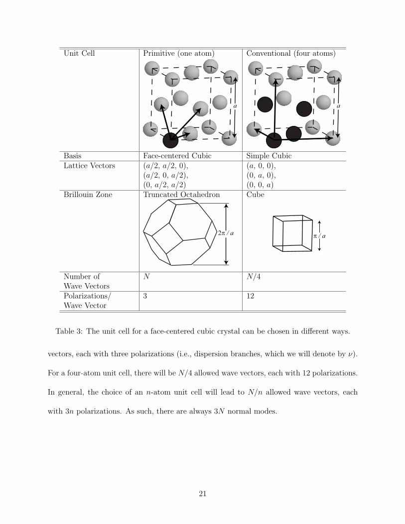
3.2 Unit Cell Specification

Harmonic lattice dynamics is a framework for determining the frequencies and mode

shapes of a linear mass-spring system. For a periodic system, the unit cell (i.e., the basis)

and lattice vectors are first specified based on the atomic structure. This specification is

not unique. For example, as shown in Table 3, one can choose a one atom-basis and a

face-centered cubic lattice (the primitive unit cell) or a four-atom basis and the simple cubic

lattice (the conventional unit cell) to describe the same structure. The unit cell choice may

be related to theoretical or computational complexity, but will not affect the bulk properties

(e.g., heat capacity or thermal conductivity).

The selection of the unit cell sets the shape of the Brillouin zone and the points that will

be resolved inside it (i.e., the allowed wave vectors, κκκ). For a simulation cell with N atoms,

there are 3N normal modes. If the unit cell has one atom, there will be N allowed wave

20

Unit Cell Primitive (one atom)

a

Conventional (four atoms)

a

Basis Face-centered Cubic Simple CubicLattice Vectors (a/2, a/2, 0),

(a/2, 0, a/2),(0, a/2, a/2)

(a, 0, 0),(0, a, 0),(0, 0, a)

Brillouin Zone Truncated Octahedron

2π / a

Cube

π / a

Number ofWave Vectors

N N/4

Polarizations/Wave Vector

3 12

Table 3: The unit cell for a face-centered cubic crystal can be chosen in different ways.

vectors, each with three polarizations (i.e., dispersion branches, which we will denote by ν).

For a four-atom unit cell, there will be N/4 allowed wave vectors, each with 12 polarizations.

In general, the choice of an n-atom unit cell will lead to N/n allowed wave vectors, each

with 3n polarizations. As such, there are always 3N normal modes.

21

3.3 Frequencies and Mode Shapes

The equation of motion of the bth atom in the lth unit cell is

mbu(lb; t) = −∑b′l′

ΦΦΦ(bl; b′l′) · u(l′

b′ ; t), (6)

where mb is the mass of atom b, ΦΦΦ is the 3×3 force constant matrix describing the interaction

between atoms bl and b′l′, u(lb; t) is the displacement of atom bl from its equilibrium position,

and the summation is over every atom in the system (including bl itself). An interatomic

potential can be used to obtain the force constants analytically [29] or numerically [30, 31].

Now assume a plane wave (i.e., harmonic) solution to Eq. (6), which will be a sum over all

the normal modes (i.e., over all wave vectors and polarizations), which have frequencies ω(κκκν):

u(lb; t) =∑κκκ,ν

1

(mbN)1/2exp{i[κκκ · ro(l0)− ω(κκκν) t]}eb(κκκν) , (7)

where ro(l0) is the equilibrium position of the lth unit cell. Substituting Eq. (7) into Eq. (6)

leads to the eigenvalue problem

ω2(κκκν) e(κκκν) = D(κκκ) · e(κκκν) , (8)

where D(κκκ) is the 3n× 3n dynamical matrix and e(κκκν) is the polarization vector of length 3n

for mode(κκκν). In Eq. (7), eb(κκκν) contains the three elements of e(κκκν) that correspond to the bth

atom of the unit cell (elements 3b− 2, 3b− 1, and 3b). The elements of D(κκκ) are given by

D3(b−1)+α,3(b′−1)+β(bb′,κκκ) =

1

(mbm′b)

1/2

∑l′

Φαβ(b0; b′l′) exp{iκκκ · [ro(l′0)− ro(l0)]}. (9)

The summation is over all unit cells and α or β equals 1 for x, 2 for y, and 3 for z. By solving

the eigenvalue problem for all allowed wave vectors, the normal mode frequencies and mode

shapes are obtained. From the frequencies, one can calculate mode specific heats using either

22

Bose-Einstein or Boltzmann statistics and build phonon dispersion curves and the density

of states. As a final point, we note that the distinction between longitudinal and transverse

mode shape polarizations is only typically possible along high symmetry directions.

3.4 Group Velocity

There are two distinct approaches for calculating the group velocity vector, which is

defined as

vg(κκκν) =

∂ω(κκκν)

∂κκκ. (10)

The first approach is to evaluate the components using the analytical expression [74]

vg,α(κκκν) =

1

2ω(κκκν)

[e†(κκκν)

∂D(κκκ)

∂κα

e(κκκν)

], (11)

where the superscript † denotes the transpose conjugate transpose.

The second approach is to perform a central difference on Eq. (10) using closely-space

wave vectors. This technique is advantageous as no additional computational framework is

needed beyond the solution of the eigenvalue problem. The disadvantage is that there is

ambiguity when performing the central difference near where two dispersion branches cross.

This ambiguity exists because eigenvalue solvers typically provide their output without any

knowledge of the specific normal modes. This challenge can be overcome by using very small

changes in the wave vector when performing the central difference and using the mode shapes

to differentiate branches. For modes at the center or edge of the Brillouin zone, a forward or

backward difference must be used. Care must also be taken near local minima or maxima,

where the group velocity is zero. Based on these issues, we recommend using Eq. (11) to

calculate the group velocity.

23

4 Normal Mode Decomposition

4.1 Formulation in Time and Frequency Domains

In normal mode decomposition [36, 37, 46, 47], the atomic positions and velocities from an

MD simulation are projected onto the normal mode coordinates of the system. The normal

mode coordinates are then used to calculate the normal mode potential and kinetic energies,

from which one can extract the normal mode lifetime. The procedure is outlined below. A

full derivation can be found in Ref. [75].

The normal mode coordinate, q(κκκν ; t), and its time derivative, q(κκκν ; t), are

q(κκκν ; t) =∑b,l

(mb

N

)1/2

exp[iκκκ · r0(l0)]e∗b(κκκν) · u(lb; t) (12)

and

q(κκκν ; t) =∑b,l

(mb

N

)1/2

exp[iκκκ · r0(l0)]e∗b(κκκν) · u(lb; t) . (13)

The potential and kinetic energies of the normal mode are

U(κκκν ; t) =1

2ω(κκκν)

2 q∗(κκκν ; t) q(κκκν ; t) (14)

and

T(κκκν ; t) =1

2q∗(κκκν ; t) q(

κκκν ; t) , (15)

such that the total energy of the normal mode is

E(κκκν ; t) = U(κκκν ; t) + T(κκκν ; t) . (16)

From lattice dynamics theory, it can be shown that [75]

⟨T(κκκν ; t)T(κκκν ; 0)⟩⟨T(κκκν ; 0)T(κκκν ; 0)⟩

= cos2[ωa(κκκν) t] exp[−2Γ(κκκν) t] (17)

24

and

⟨E(κκκν ; t)E(κκκν ; 0)⟩⟨E(κκκν ; 0)E(κκκν ; 0)⟩

= exp[−2Γ(κκκν) t], (18)

where ωa is the anharmonic frequency (as opposed to that predicted from harmonic lattice

dynamics) and Γ(κκκν) is the line width, equal to 1/[2τ(κκκν)].5 Thus, one can find the lifetime

by fitting the normalized autocorrelation of the mode total energy to an exponential decay.

Instead of fitting an exponential function, the lifetime can be approximated as

τ(κκκν) =

∫ ∞

0

⟨E(κκκν ; t)E(κκκν ; 0)⟩⟨E(κκκν ; 0)E(κκκν ; 0)⟩

dt, (19)

an expression that is beneficial when studying disordered systems.

Normal mode decomposition can also be performed in the frequency domain. The ex-

pectation value of the mode kinetic energy is

⟨T(κκκν)⟩ = limτ0→∞

1

2τ0

∫ τ0

0

q∗(κκκν ; t) q(κκκν ; t) dt. (20)

Using the Parseval theorem [76], Eq. (20) can be transformed to be frequency domain, giving

T(κκκν ;ω) = limτ0→∞

1

2τ0

∣∣∣∣ 1√2π

∫ τ0

0

q(κκκν ; t) exp(−iωt)dt

∣∣∣∣2 . (21)

Under the assumption of equipartition of energy, which is good for classical MD simulations

[46, 47],

E(κκκν ;ω) = 2T(κκκν ;ω) . (22)

Through the Wiener-Khinchin theorem [76], Eq. (17) can be recast in the frequency domain

leading to the Lorentzian function

E(κκκν ;ω) = C(κκκν)Γ(κκκν) /π

[ωa(κκκν)− ω]2 + Γ2(κκκν)

, (23)

5The factor of two in the relationship between the line width and the lifetime arises because the analysis

is performed on the normal mode energy and not on the normal mode coordinate.

25

where C(κκκν) is a mode-dependent constant. The phonon frequency and line width can be

extracted by fitting Eq. (21), as obtained from MD simulation, to a Lorentzian function.

Normal mode decomposition therefore proceeds as follows:

1. Choose the unit cell and build the atomic structure (i.e., the simulation cell).

2. Specify the allowed wave vectors for the simulation cell.

3. Perform quasi-harmonic lattice dynamics calculations to obtain the frequencies and

mode shapes of all normal modes.

4. Run MD simulations, outputting the atomic positions and velocities.

5. Project the atomic positions and velocities onto the normal mode coordinates [Eqs. (12)

and (13)].

6. For time-domain analysis, calculate the autocorrelation of the kinetic and/or total

normal mode energies, and extract the phonon properties from Eqs. (17), (18), and/or

(19).

7. For frequency-domain analysis, calculate Eq. (21) for a range of frequencies around

the harmonic frequency for each normal mode and extract the phonon properties from

Eq. (23). Alternatively, perform a Fourier transform on the kinetic energy autocorre-

lation, the left side of Eq. (17), and extract the phonon properties from Eq. (23).

Note that the lifetimes obtained from normal mode decomposition contain the combined

effects of normal and Umklapp processes. While the frequency- and time-domain approaches

are equivalent, we will demonstrate in the following sections that one may be preferred

depending on the system being studied.

26

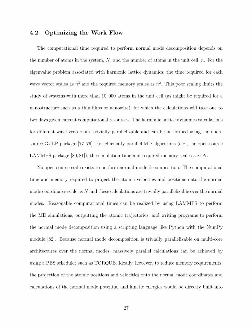
4.2 Optimizing the Work Flow

The computational time required to perform normal mode decomposition depends on

the number of atoms in the system, N , and the number of atoms in the unit cell, n. For the

eigenvalue problem associated with harmonic lattice dynamics, the time required for each

wave vector scales as n3 and the required memory scales as n2. This poor scaling limits the

study of systems with more than 10, 000 atoms in the unit cell (as might be required for a

nanostructure such as a thin films or nanowire), for which the calculations will take one to

two days given current computational resources. The harmonic lattice dynamics calculations

for different wave vectors are trivially parallelizable and can be performed using the open-

source GULP package [77–79]. For efficiently parallel MD algorithms (e.g., the open-source

LAMMPS package [80, 81]), the simulation time and required memory scale as ∼ N .

No open-source code exists to perform normal mode decomposition. The computational

time and memory required to project the atomic velocities and positions onto the normal

mode coordinates scale asN and these calculations are trivially parallelizable over the normal

modes. Reasonable computational times can be realized by using LAMMPS to perform

the MD simulations, outputting the atomic trajectories, and writing programs to perform

the normal mode decomposition using a scripting language like Python with the NumPy

module [82]. Because normal mode decomposition is trivially parallelizable on multi-core

architectures over the normal modes, massively parallel calculations can be achieved by

using a PBS scheduler such as TORQUE. Ideally, however, to reduce memory requirements,

the projection of the atomic positions and velocities onto the normal mode coordinates and

calculations of the normal mode potential and kinetic energies would be directly built into

27

the MD code. The energies would then be periodically output to perform the required

autocorrelations and/or Fourier transforms.

In normal mode decomposition, the sampling rate must be high enough to capture the

maximum frequency in the system. The sampling rate and total run time should be chosen

in powers of two as a convenience in performing fast Fourier transforms. Obtaining the

phonon properties from Eqs. (17), (18), (19), and (23) requires specification of a time or

frequency range and initial guesses for the frequency and lifetime. These parameters can be

obtained from observation of the raw data. An initial guess for the frequency can also be

obtained from the harmonic lattice dynamics calculations. When investigating new systems,

it is best to fit the phonon properties in a semi-automated way (i.e., each fit should be

visualized so that the fitting parameters can be tuned). Once appropriate fitting parameters

are chosen, the fitting can usually be fully automated for large data sets. For crystalline

systems, only the properties of the modes of the irreducible wave vectors are needed, such

that the autocorrelations or Fourier transforms for symmetric modes can be averaged before

fitting.

4.3 Case Study: Lennard-Jones Crystal

Having described the normal mode decomposition theoretical approach and computa-

tional methodology in Sections 4.1 and 4.2, we now carry out a case study on a LJ crystal

at a dimensionless temperature of 0.0827 (corresponding to an argon temperature of 10 K).

While this temperature is low (the LJ argon Debye temperature is around 85 K), it will allow

for a clean demonstration of the technique. The LJ interatomic potential is computationally

inexpensive and is thus ideal for use in code development and testing. All results will be

28

presented in dimensionless LJ units [48]. The zero pressure lattice constant is 1.556 (Ref.

[83]) and the potential energy is cutoff and shifted at a distance of 2.5.

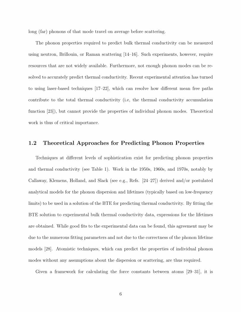
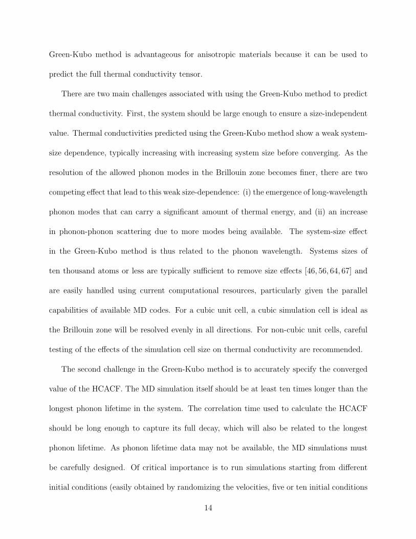
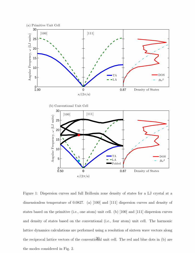
From the same simulation cell and atomic data, one can perform normal mode decom-

position on either the primitive or conventional unit cells.6 The [100] and [111] dispersion

curves and density of states obtained from harmonic lattice dynamics calculations are plot-

ted for each unit cell in Figs. 1(a) and (b). While the dispersion curves in each direction

show similarities, they are necessarily different due to the allowed wave vectors and shape of

the Brillouin zone (see Table 3). The density of states, however, are identical, as expected

and required. We note that the conventional unit cell description leads to what appear to

be optical modes. In reality, these modes are a result of zone folding and can be mapped

directly to acoustic modes in the primitive unit cell description.

The MD simulations are run in the NV E ensemble, the dimensionless time step is 0.002,

and the equations of motion are integrated using the velocity Verlet algorithm. The system

is equilibrated for 220 time steps before collecting data every 25 time steps for an additional

220 time steps. In order to capture system-size effects, cubic simulation cells with between

256 and 6912 atoms are considered (corresponding to between four and twelve conventional

unit cells, No, in each of the x, y, and z directions). Ten simulations are performed with

different initial velocities and the autocorrelations (or Fourier transforms) are averaged over

the initial conditions and symmetric wave vectors before fitting the phonon properties.

6The allowed wave vectors are defined by the basis and the supercell used to perform the MD simulations.

For a supercell built using the conventional unit cell, as we use, the allowed wave vectors can be labeled

using either the conventional or primitive unit cell description. For a supercell built using the primitive unit

cell, however, all wave vectors cannot be labeled using the conventional unit cell description.

29

5

10

15

20

25

Density of States

0 0.87

5

10

15

20

25

1.000

5

10

15

20

25

30

κ/(2π/a)

Angula

rFre

quen

cy,ω

(LJ

unit

s)

DOS

Bω2

TA

LA

[111][100]

(a) Primitive Unit Cell

5

10

15

20

25

Density of States

0 0.87

5

10

15

20

25

00.500

5

10

15

20

25

30

κ/(2π/a)

Angula

rFre

quen

cy,ω

(LJ

unit

s)

TA

LA

Folded

DOS

Bω2

[100] [111]

(b) Conventional Unit Cell

B

A

Figure 1: Dispersion curves and full Brillouin zone density of states for a LJ crystal at a

dimensionless temperature of 0.0827. (a) [100] and [111] dispersion curves and density of

states based on the primitive (i.e., one atom) unit cell. (b) [100] and [111] dispersion curves

and density of states based on the conventional (i.e., four atom) unit cell. The harmonic

lattice dynamics calculations are performed using a resolution of sixteen wave vectors along

the reciprocal lattice vectors of the conventional unit cell. The red and blue dots in (b) are

the modes considered in Fig. 2.

30

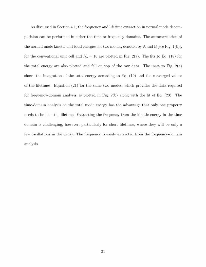
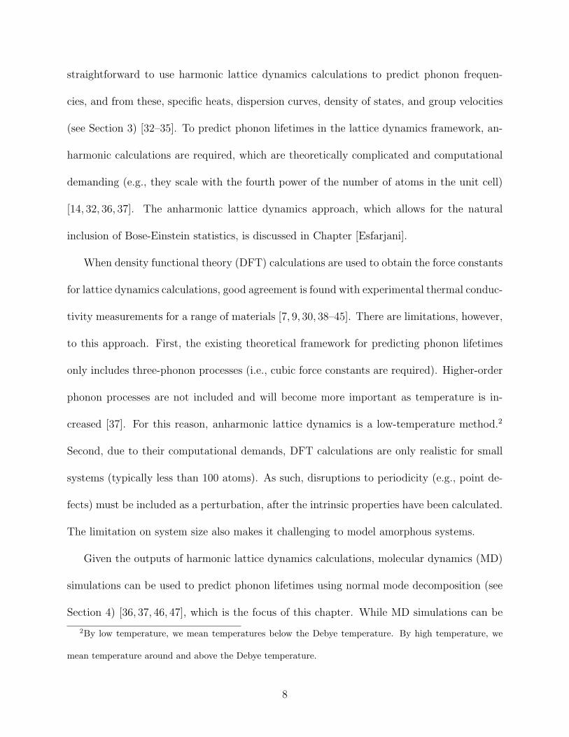
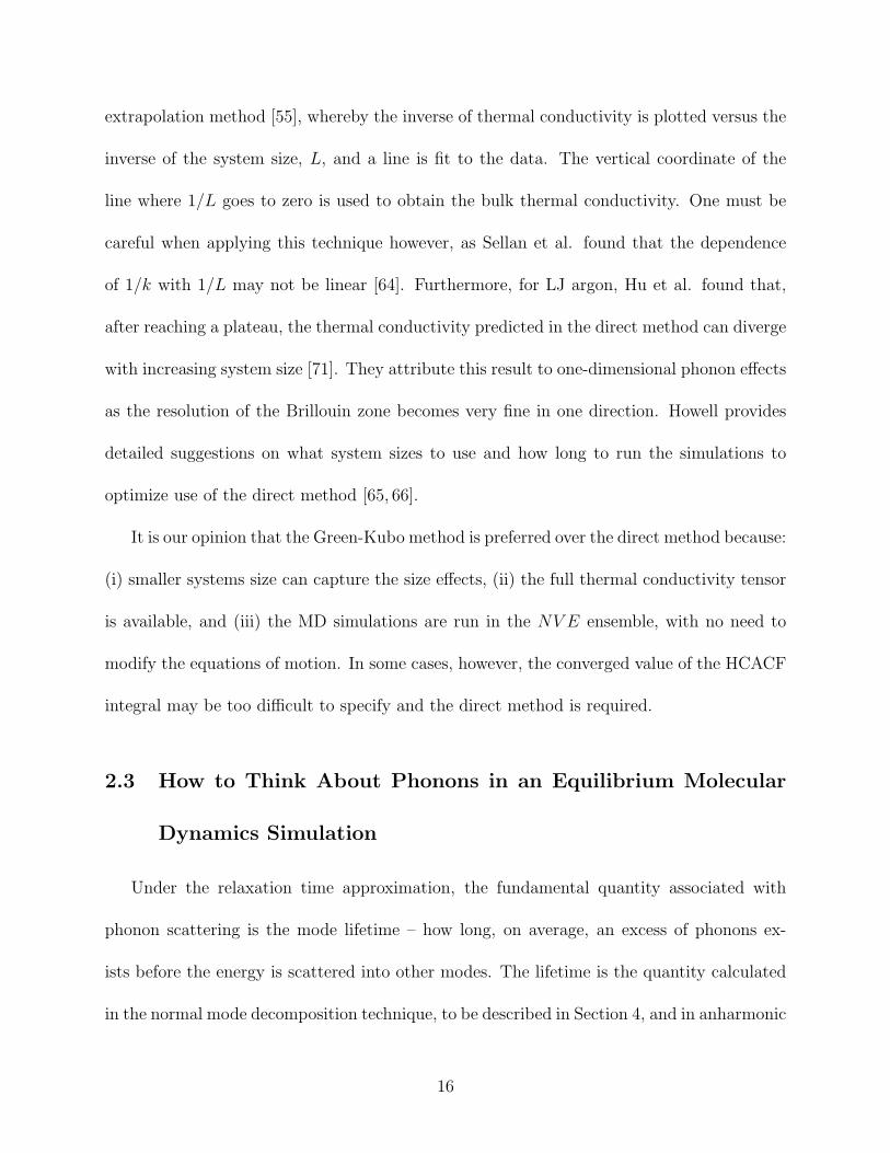
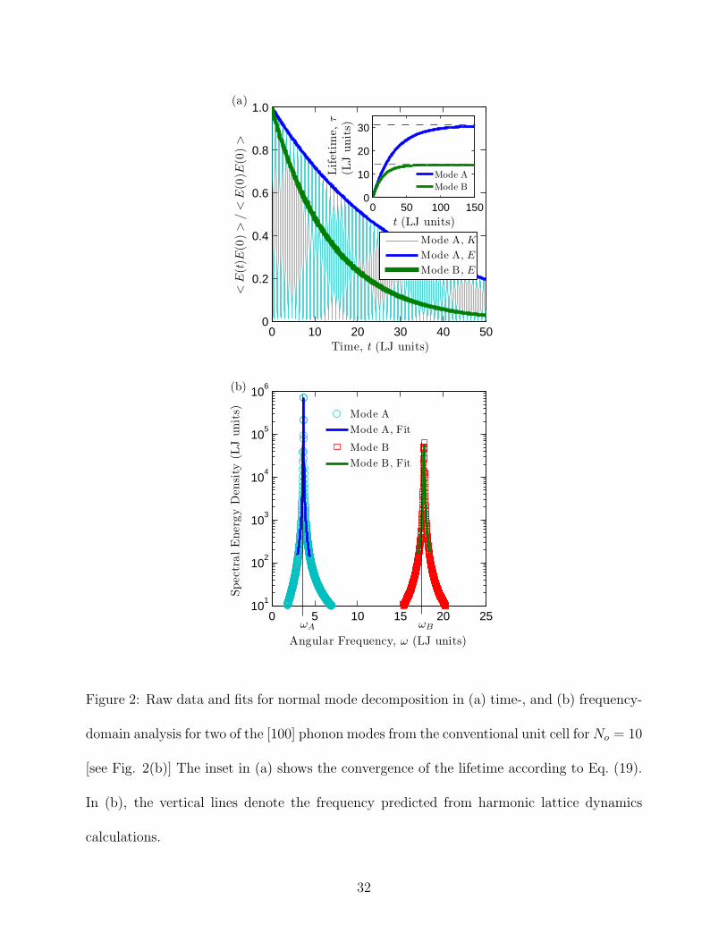
As discussed in Section 4.1, the frequency and lifetime extraction in normal mode decom-

position can be performed in either the time or frequency domains. The autocorrelation of

the normal mode kinetic and total energies for two modes, denoted by A and B [see Fig. 1(b)],

for the conventional unit cell and No = 10 are plotted in Fig. 2(a). The fits to Eq. (18) for

the total energy are also plotted and fall on top of the raw data. The inset to Fig. 2(a)

shows the integration of the total energy according to Eq. (19) and the converged values

of the lifetimes. Equation (21) for the same two modes, which provides the data required

for frequency-domain analysis, is plotted in Fig. 2(b) along with the fit of Eq. (23). The

time-domain analysis on the total mode energy has the advantage that only one property

needs to be fit – the lifetime. Extracting the frequency from the kinetic energy in the time

domain is challenging, however, particularly for short lifetimes, where they will be only a

few oscillations in the decay. The frequency is easily extracted from the frequency-domain

analysis.

31

0 10 20 30 40 500

0.2

0.4

0.6

0.8

1.0

Time, t (LJ units)

<E

(t)E

(0)

>/

<E

(0)E

(0)

>

0 50 100 1500

10

20

30

t (LJ units)

Lifet

ime,

τ(L

Junit

s)

Mode A

Mode B

Mode A, K

Mode A, E

Mode B, E

(a)

0 5 10 15 20 2510

1

102

103

104

105

106

Angular Frequency, ω (LJ units)

Spec

tralE

ner

gy

Den

sity

(LJ

unit

s)

Mode A

Mode A, Fit

Mode B

Mode B, Fit

ωBωA

(b)

Figure 2: Raw data and fits for normal mode decomposition in (a) time-, and (b) frequency-

domain analysis for two of the [100] phonon modes from the conventional unit cell forNo = 10

[see Fig. 2(b)] The inset in (a) shows the convergence of the lifetime according to Eq. (19).

In (b), the vertical lines denote the frequency predicted from harmonic lattice dynamics

calculations.

32

The anharmonic frequencies (3.68 and 17.8) are close to the frequencies obtained from

harmonic lattice dynamics calculations (3.70 and 17.5). At this low temperature, the shift in

frequency away from the quasi-harmonic value is small and can be neglected when calculating

the group velocity. At higher temperatures, however, as the LJ system is soft, the frequency

shift becomes appreciable [37, 46]. For stiffer systems like silicon, the frequency shift is small

and is often neglected [39, 60]. Due to the coarse resolution of the Brillouin zone in the MD

simulations, the group velocity cannot be accurately specified. As such, we recommend using

the group velocities from harmonic lattice dynamics calculations in thermal conductivity

prediction (see Section 3.4). The lifetimes from the time-domain analysis (30.5 and 13.9)

and the frequency-domain analysis (32.5 and 13.4) are within 10% of each other, which is

representative of what we find for modes from the full Brillouin zone. We attribute the

differences to the non-linear fitting procedures.

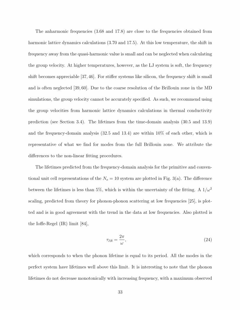
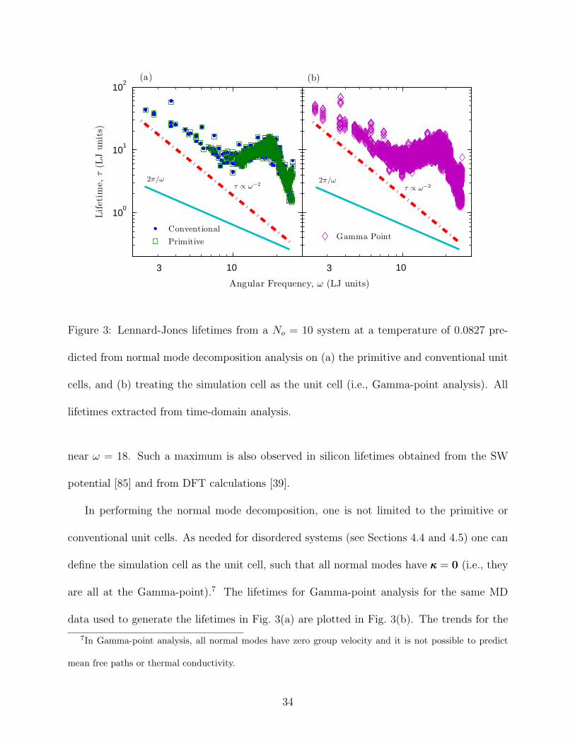
The lifetimes predicted from the frequency-domain analysis for the primitive and conven-

tional unit cell representations of the No = 10 system are plotted in Fig. 3(a). The difference

between the lifetimes is less than 5%, which is within the uncertainty of the fitting. A 1/ω2

scaling, predicted from theory for phonon-phonon scattering at low frequencies [25], is plot-

ted and is in good agreement with the trend in the data at low frequencies. Also plotted is

the Ioffe-Regel (IR) limit [84],

τIR =2π

ω, (24)

which corresponds to when the phonon lifetime is equal to its period. All the modes in the

perfect system have lifetimes well above this limit. It is interesting to note that the phonon

lifetimes do not decrease monotonically with increasing frequency, with a maximum observed

33

101

100

101

101

100

101

102

Angular Frequency, ω (LJ units)

Lifet

ime,

τ(L

Junit

s)

Conventional

PrimitiveGamma Point

(a) (b)

τ ∝ ω−2τ ∝ ω−2

2π/ω 2π/ω

3 3

Figure 3: Lennard-Jones lifetimes from a No = 10 system at a temperature of 0.0827 pre-

dicted from normal mode decomposition analysis on (a) the primitive and conventional unit

cells, and (b) treating the simulation cell as the unit cell (i.e., Gamma-point analysis). All

lifetimes extracted from time-domain analysis.

near ω = 18. Such a maximum is also observed in silicon lifetimes obtained from the SW

potential [85] and from DFT calculations [39].

In performing the normal mode decomposition, one is not limited to the primitive or

conventional unit cells. As needed for disordered systems (see Sections 4.4 and 4.5) one can

define the simulation cell as the unit cell, such that all normal modes have κκκ = 0 (i.e., they

are all at the Gamma-point).7 The lifetimes for Gamma-point analysis for the same MD

data used to generate the lifetimes in Fig. 3(a) are plotted in Fig. 3(b). The trends for the

7In Gamma-point analysis, all normal modes have zero group velocity and it is not possible to predict

mean free paths or thermal conductivity.

34

Gamma-point analysis are the same as for the primitive and conventional unit cells. There

is more scatter in the Gamma-point data as wave vector symmetry averaging is no longer

possible.

The phonon properties obtained from normal mode decomposition and harmonic lattice

dynamics calculations can now be used to predict bulk thermal conductivity using Eq. (2).

For classical MD simulations the assumption of equipartition of energy is very good and we

take the volumetric specific heat to be kB/V for all modes [46, 47, 86].

The Gamma point corresponds to bulk translation and therefore does not contribute to

thermal conductivity. By discretizing the Brillouin zone, we assign a volume to the Gamma

point. The zero contribution of this volume to the thermal conductivity introduces a size

effect in the prediction. To predict a bulk thermal conductivity, an extrapolation procedure

is used, whereby k is plotted versus 1/No and a line is fit to the data. The point on this line

where 1/No = 0 gives the bulk thermal conductivity [37, 39]. This extrapolation procedure

requires that the low-frequency modes be dominated by intrinsic scattering (i.e., τ ∝ ω−2)

and have a similar group velocity [39, 41]. For the LJ crystal, this requirement is satisfied for

modest system sizes (No ≥ 6). The size-dependent and extrapolated thermal conductivities

are plotted in Fig. 4 for both the primitive and conventional unit cells. The Green-Kubo

predictions for the same system are also plotted and show no size effect, consistent with

previous work [46].

The extrapolated thermal conductivities from the primitive and conventional unit cells

are 177±15 and 176±14 W/m-K. The Green-Kubo thermal conductivity is 173±13 W/m-K.

All thermal conductivities agree well within their respective uncertainties.

For the perfect LJ crystal, there is no clear advantage of performing the analysis in the

35

0 0.1 0.2 0.3 150

160

170

180

190

1/N0

Ther

malC

onduct

ivit

y,k

(LJ

unit

s)

GK

NMD Conventional

NMD Primitive

Figure 4: Size dependence of thermal conductivity for the LJ crystal at a temperature of

0.0827 from normal mode decomposition and the Green-Kubo method.

time or frequency domains or for the primitive or conventional unit cells. Challenges may

emerge for high thermal conductivity materials like silicon or carbon nanotubes, where the

time-domain decay may not be well described by an exponential and the peaks in frequency

space get narrow or are not well-fit by a Lorentzian. The failure of the fitting for a perfect

crystal is an indication that the relaxation time approximation may not be appropriate

and that care should be taken when interpreting the results. In general, new materials

should be investigated on a case-by-case basis to determine the approach that minimizes the

uncertainty.

36

4.4 Application to Alloys

In Section 4.3, we showed how normal mode decomposition is applied to a perfect crystal.

In reality, any crystal will have some deviation from perfect periodicity, which may be caused

by a point defect, a dislocation, a grain boundary, or a free surface. In extreme cases, these

deviations from periodicity will lead to the emergence of modified normal modes. For small

perturbations, however, it is reasonable to assume that the frequencies and mode shapes of

the normal modes will be unchanged and that the effect of the perturbation will be on the

lifetimes. Under this assumption, one can still project the atomic positions and velocities

onto the normal modes of the unperturbed system.

In this section, we explore the validity of normal mode decomposition for modeling an

alloy. In an alloy, the atomic positions follow those of a crystal lattice, but the placement of

the atomic species is random. It has been argued that the dominant effect of alloying atoms

is due to their mass mismatch with the host lattice [87, 88]. Changes in local bond stiffness

are expected to be a secondary effect. As such, we create two alloy systems by randomly

changing the masses of 5 and 50% of the atoms in the perfect LJ crystal to three times the

LJ mass. The MD simulation parameters are identical to those for the perfect crystal.

While one could perform the normal mode decomposition by projecting the atomic posi-

tions and velocities onto the modes of the unperturbed system, it is more appropriate to use

the virtual crystal approximation [40, 42, 43, 89]. Under the virtual crystal approximation,

the system is replaced by one where all atoms have the same mass, equal to the average of

the atomic masses in the system of interest. This system will have the same mode shapes

as the original system, but the frequencies are modified due to the change in the average

37

atomic mass.

Results for the time- and frequency domain approaches to normal mode decomposition

are shown for two modes in Figs. 5(a)-(d). These two modes are equivalent to those shown

in the perfect crystal case study in Figs. 1(b), 2(a), and 2(b). For a concentration, c, of 0.05,

both peaks in the frequency domain are well-formed and a lifetime can be extracted by fitting

the data to a Lorentzian function. This behavior is typical of all modes at a concentration

of 0.05. The downward frequency shift is related to the increased average atomic mass.

For an alloy concentration of 0.5, the lower frequency mode still has a well-formed peak.

The higher-frequency mode does not, however, such that a lifetime cannot be extracted by

fitting to a Lorentzian function. Such behavior is typical of the higher frequency modes

at high alloy concentrations. This change in behavior is also seen in the time domain,

where the decay of the autocorrelation of the total mode energy is no longer a smooth

exponential function. This behavior indicates that the virtual crystal normal mode is not

a good description of the true normal mode. As such, we use Eq. (19) to approximate a

lifetime, as shown in Figs. 5(c) and 5(d).

38

0 5 10 15 20 25

102

104

106

Angular Frequency, ω (LJ units)

Spec

tralE

ner

gy

Den

sity

(LJ

unit

s)

Mode A, c = 0.0

Mode A, c = 0.05

Mode A, c = 0.5

Mode B, c = 0.0

Mode B, c = 0.05

Mode B, c = 0.5

(a)

0 2 4 60

0.2

0.4

0.6

0.8

1.0

Time, t (LJ units)

<E

(t)E

(0)

>/

<E

(0)E

(0)

>

0 100 2000

20

40

Time, t (LJ units)

Lifet

ime,

τ(L

Junit

s)

0 2 40

0.3

0.6

Time, t (LJ units)

Mode BMode A

(b)

(d)(c)

Mode A, KMode A, EMode B, KMode B, E

Figure 5: Virtual crystal (a) frequency-domain and (b) time-domain normal mode decompo-

sition analysis for two modes in LJ alloys with concentrations of 0.05 and 0.5. For modes that

are not well-approximated by the virtual crystal modes, the lifetime can be approximated

using Eq. (19), as shown in (d).

39

101

10−1

100

101

102

Angular Frequency, ω (LJ units)

Lifet

ime,

τ(L

Junit

s)

NMD c=0.0Gamma Point c=0.05VC-NMD c=0.05

τ ∝ ω−2

3

τ ∝ ω−4

2π/ω

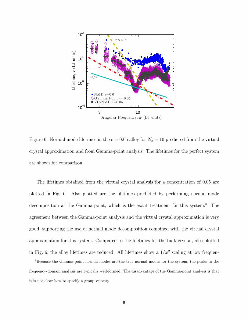
Figure 6: Normal mode lifetimes in the c = 0.05 alloy for No = 10 predicted from the virtual

crystal approximation and from Gamma-point analysis. The lifetimes for the perfect system

are shown for comparison.

The lifetimes obtained from the virtual crystal analysis for a concentration of 0.05 are

plotted in Fig. 6. Also plotted are the lifetimes predicted by performing normal mode

decomposition at the Gamma-point, which is the exact treatment for this system.8 The

agreement between the Gamma-point analysis and the virtual crystal approximation is very

good, supporting the use of normal mode decomposition combined with the virtual crystal

approximation for this system. Compared to the lifetimes for the bulk crystal, also plotted

in Fig. 6, the alloy lifetimes are reduced. All lifetimes show a 1/ω2 scaling at low frequen-

8Because the Gamma-point normal modes are the true normal modes for the system, the peaks in the

frequency-domain analysis are typically well-formed. The disadvantage of the Gamma-point analysis is that

it is not clear how to specify a group velocity.

40

0 0.1 0.2 0.3

32

38

44

1/N0

Ther

malC

onduct

ivit

y,k

(LJ

unit

s)

GK, c=0.05

VC-NMD, c=0.05

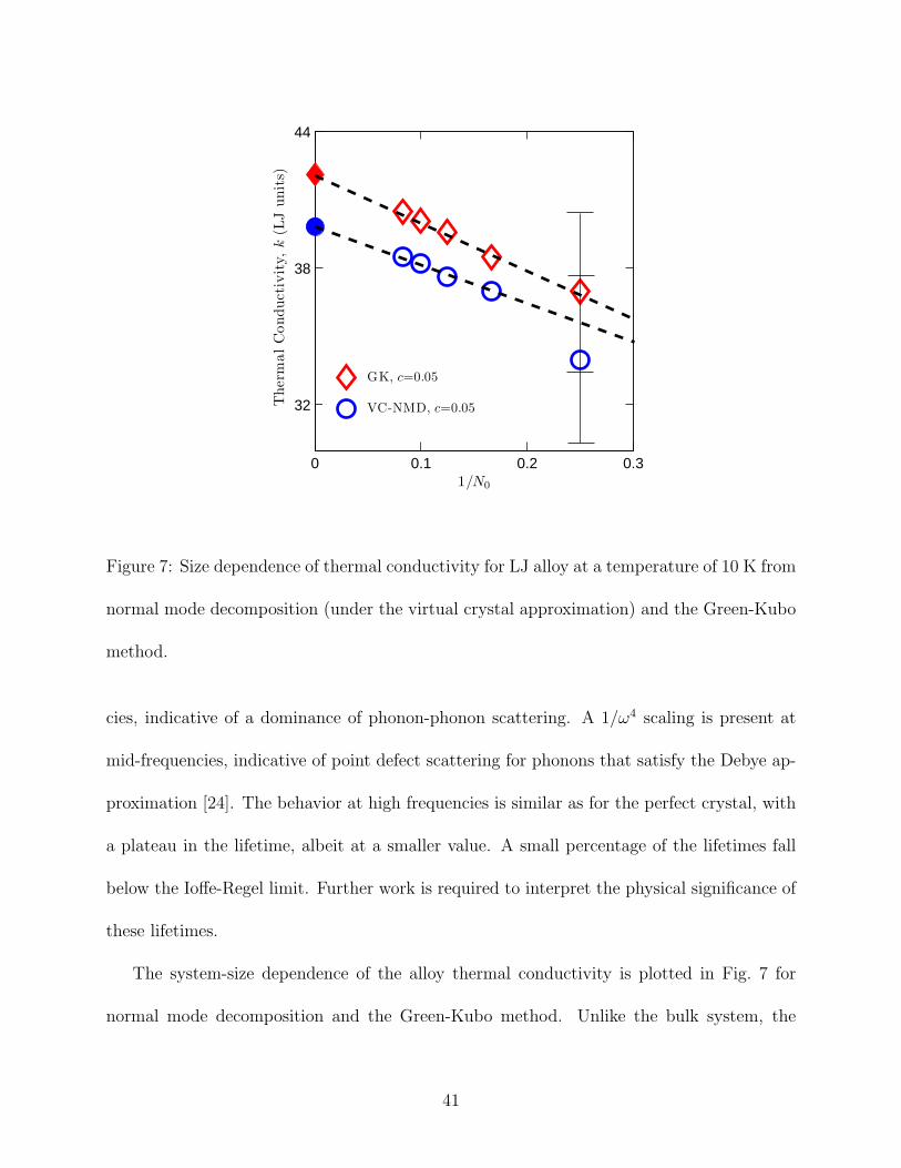
Figure 7: Size dependence of thermal conductivity for LJ alloy at a temperature of 10 K from

normal mode decomposition (under the virtual crystal approximation) and the Green-Kubo

method.

cies, indicative of a dominance of phonon-phonon scattering. A 1/ω4 scaling is present at

mid-frequencies, indicative of point defect scattering for phonons that satisfy the Debye ap-

proximation [24]. The behavior at high frequencies is similar as for the perfect crystal, with

a plateau in the lifetime, albeit at a smaller value. A small percentage of the lifetimes fall

below the Ioffe-Regel limit. Further work is required to interpret the physical significance of

these lifetimes.

The system-size dependence of the alloy thermal conductivity is plotted in Fig. 7 for

normal mode decomposition and the Green-Kubo method. Unlike the bulk system, the

41

Green-Kubo data show a surprising size dependence that requires further study. Also of note

is that the normal mode decomposition point at No = 4 does not follow the linear trend,

suggesting that this system size is not large enough to satisfy the requirements needed for the

linear extrapolation procedure (i.e., the phonon scattering at low frequencies is dominated

by phonon-phonon interactions). The extrapolated normal mode decomposition and Green-

Kubo thermal conductivities are 40 ± 6 and 42 ± 4. The systematic under-prediction by

normal mode decomposition is most likely related to the virtual crystal approximation.

This application of normal mode decomposition to a mass-based alloy is straightforward

because the equilibrium atomic positions do not change. For other point defects (e.g., a

vacancy), more care will need to be taken to assess if the virtual crystal normal modes are

a good approximation for the perturbed system.

4.5 Application to Amorphous Solids

For systems with a large degree of disorder, the normal mode analysis can always be

performed by treating the simulation cell as the unit cell (i.e., Gamma-point analysis). This

approach has the disadvantage of not being able to provide a phonon group velocity, such

that it is not possible to predict a mean free path or thermal conductivity. That being said,

the analysis still allows for an understanding of relevant time scales and assistance in the

identification of non-phonon like modes.[90]

We now perform a case study on an amorphous LJ system at a dimensionless tempera-

ture of 0.0413. The amorphous solid is generated by liquifying the crystal, instantaneously

removing all kinetic energy, and then relaxing the structure. The MD simulation parameters

42

are the same as for the crystal and alloy. One system with 2048 atoms is modeled. The

LJ amorphous solid is metastable at this temperature and intermittently moves between

very similar low-energy states. Evidence for the metastability can be found by analyzing

the time-histories of the atomic displacements. As such, normal mode decomposition, which

requires the average atomic positions, will be an approximation.

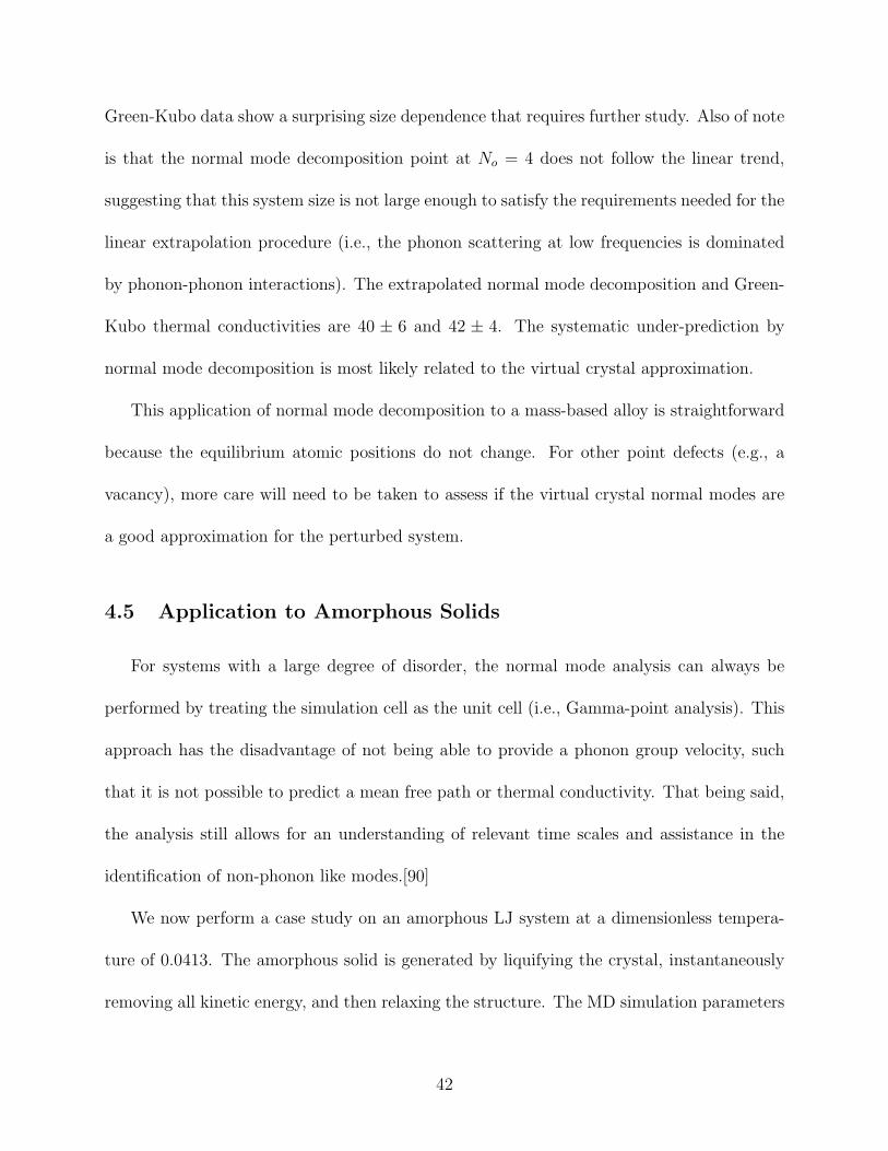
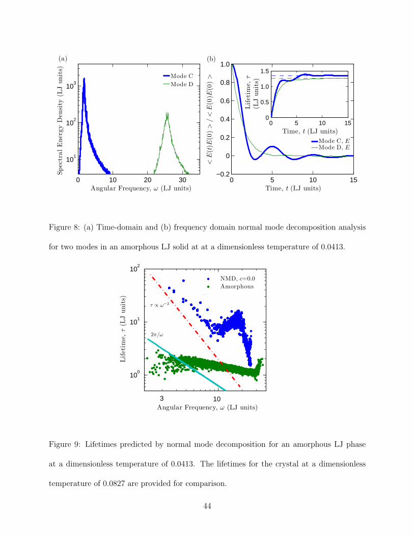
The time- and frequency-domain approaches to normal mode decomposition are shown

for two mode in the amorphous system in Figs. 8(a) and 8(b). Because the analysis is

performed at the Gamma-point, the peaks are well formed, but they are not Lorentzian,

which may be due to non-plane wave behavior. We believe that the oscillations in the total

energy correlation for the low frequency mode is a consequence of the metastability of the

amorphous phase. As such, we extract the lifetimes by using Eq. (19), as shown in the inset

to Fig. 8(b).

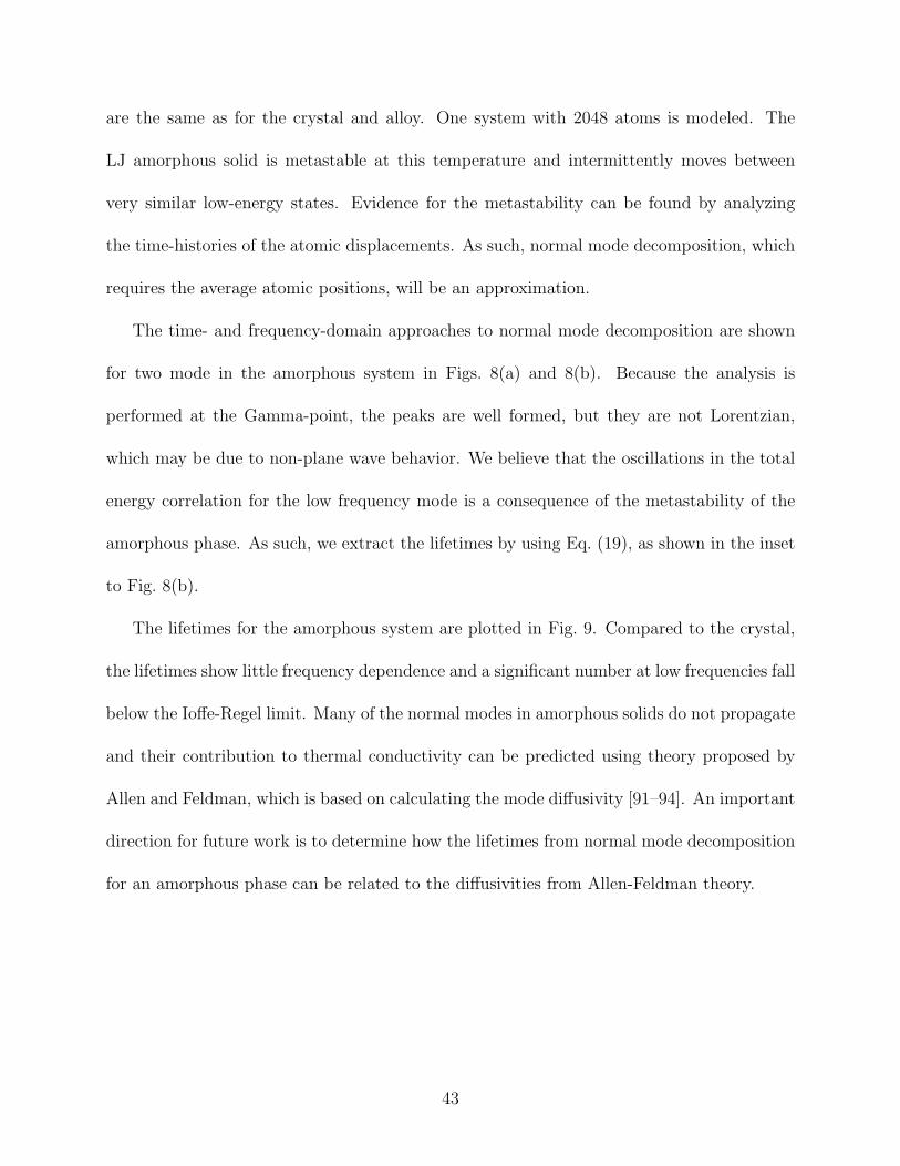
The lifetimes for the amorphous system are plotted in Fig. 9. Compared to the crystal,

the lifetimes show little frequency dependence and a significant number at low frequencies fall

below the Ioffe-Regel limit. Many of the normal modes in amorphous solids do not propagate

and their contribution to thermal conductivity can be predicted using theory proposed by

Allen and Feldman, which is based on calculating the mode diffusivity [91–94]. An important

direction for future work is to determine how the lifetimes from normal mode decomposition

for an amorphous phase can be related to the diffusivities from Allen-Feldman theory.

43

0 10 20 30

101

102

103

Angular Frequency, ω (LJ units)

Spec

tralE

ner

gy

Den

sity

(LJ

unit

s)

0 5 10 15−0.2

0.2

0.4

0.6

0.8

1.0

0

Time, t (LJ units)

<E

(t)E

(0)

>/

<E

(0)E

(0)

>

0 5 10 150

0.5

1.0

1.5

Time, t (LJ units)

Lifet

ime,

τ(L

Junit

s)

Mode C

Mode D

Mode C, EMode D, E

(a) (b)

Figure 8: (a) Time-domain and (b) frequency domain normal mode decomposition analysis

for two modes in an amorphous LJ solid at at a dimensionless temperature of 0.0413.

101

100

101

102

Angular Frequency, ω (LJ units)

Lifet

ime,

τ(L

Junit

s)

NMD, c=0.0

Amorphous

3

τ ∝ ω−2

2π/ω

Figure 9: Lifetimes predicted by normal mode decomposition for an amorphous LJ phase

at a dimensionless temperature of 0.0413. The lifetimes for the crystal at a dimensionless

temperature of 0.0827 are provided for comparison.

44

4.6 Trajectory-based Approaches

Frequency-space techniques for predicting phonon properties that only use the atomic

velocities from an MD simulation have been proposed [95, 96]. These trajectory-based ap-

proaches are advantageous compared to normal mode decomposition due to reduced post-

processing time, as the atomic velocities are projected onto the allowed wave vectors as

opposed to onto every normal mode. Also, very large unit cells can be considered as har-

monic lattice dynamics calculations are not required and the predicted lifetimes can natu-

rally contain the effects of both intrinsic [41, 96, 97] and disorder scattering [96, 98, 99]. An

example of such a technique was first used to predict the phonon dispersion curves of car-

bon nanotubes [100]. Inconsistencies in the phonon lifetimes, however, are observed when

comparing this approach to the formally correct normal mode decomposition method and

to thermal conductivities predicted from the Green-Kubo method [47]. Results predicted

from trajectory-based approaches should therefore only be interpreted qualitatively and with

caution.

45

5 Notable Work

In 1986, Ladd et al. were the first to use normal mode decomposition [36]. They predicted

phonon frequencies, lifetimes, and thermal conductivity of a face-centered cubic crystal de-

scribed by an inverse twelfth-power interatomic potential. In this seminal paper, they also

used anharmonic lattice dynamics calculations and the Green-Kubo method, finding reason-

able agreement between the different techniques.

Almost twenty years later, McGaughey and Kaviany predicted phonon frequencies and

lifetimes for LJ argon in the [100] direction using normal mode decomposition between

temperatures of 20 and 80 K [46]. As temperature increased, they observed significant

frequency shifts and an increase in the number of lifetimes below the Ioffe-Regel limit. Size

effects in the thermal conductivity prediction were captured by fitting the lifetimes for three

system sizes (No = 4, 5, and 6) to algebraic expressions, allowing for an analytical integral

from the Gamma point to the edge of the Brillouin zone. Under the isotropic approximation,

their predicted thermal conductivities were about half of the values predicted from the

Green-Kubo method (please consult the Erratum to this paper and Ref. [37]). This finding

highlights the importance of considering modes from the entire Brillouin zone for the LJ

system.

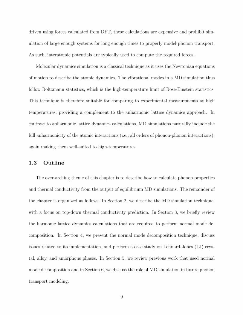
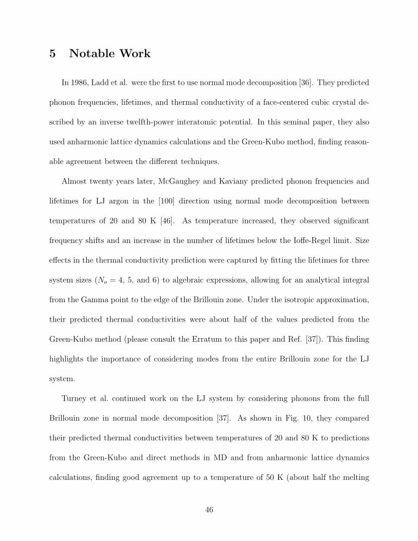
Turney et al. continued work on the LJ system by considering phonons from the full

Brillouin zone in normal mode decomposition [37]. As shown in Fig. 10, they compared

their predicted thermal conductivities between temperatures of 20 and 80 K to predictions

from the Green-Kubo and direct methods in MD and from anharmonic lattice dynamics

calculations, finding good agreement up to a temperature of 50 K (about half the melting

46

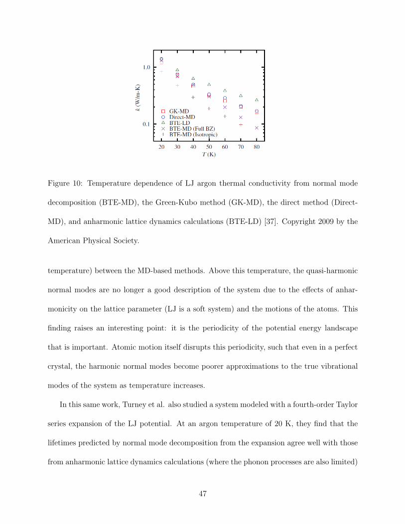
Figure 10: Temperature dependence of LJ argon thermal conductivity from normal mode

decomposition (BTE-MD), the Green-Kubo method (GK-MD), the direct method (Direct-

MD), and anharmonic lattice dynamics calculations (BTE-LD) [37]. Copyright 2009 by the

American Physical Society.

temperature) between the MD-based methods. Above this temperature, the quasi-harmonic

normal modes are no longer a good description of the system due to the effects of anhar-

monicity on the lattice parameter (LJ is a soft system) and the motions of the atoms. This

finding raises an interesting point: it is the periodicity of the potential energy landscape

that is important. Atomic motion itself disrupts this periodicity, such that even in a perfect

crystal, the harmonic normal modes become poorer approximations to the true vibrational

modes of the system as temperature increases.

In this same work, Turney et al. also studied a system modeled with a fourth-order Taylor

series expansion of the LJ potential. At an argon temperature of 20 K, they find that the

lifetimes predicted by normal mode decomposition from the expansion agree well with those

from anharmonic lattice dynamics calculations (where the phonon processes are also limited)

47

and from the full potential using normal mode decomposition. At a temperature of 50 K,

however, the lifetimes predicted from normal mode decomposition from the expansion are

higher than those from the full potential, but still in reasonable agreement with those from

anharmonic lattice dynamics calculations. This result confirms the increasing importance of

higher-order phonon processes as temperature is increased.

Using the EDIP model for silicon, Henry and Chen used normal mode decomposition to

predict phonon lifetimes for the [100], [110], and [111] directions [101]. They found a small

directional dependence, suggesting that the isotropic approximation is reasonable for silicon.

Sellan et al. later argued that the success of the isotropic approximation for silicon is possible

because the vast majority (90% or more) of the heat is carried by low-frequency acoustic

phonons [102]. Henry and Chen also found that phonons with mean free paths exceeding

one micron contribute significantly to thermal conductivity at a temperature of 300 K, a

finding supported by recent experimental work [19, 20]. Goicochea et al. [86], Zhao and

Freund [103], and Hori et al. [104] also studied silicon using normal mode decomposition.

Other bulk crystals that have been studied using normal mode decomposition include PbTe

[97], Bi2Te3 [105], and GaAs (where the input came from MD simulations driven by DFT

calculations) [106].

Donadio and Galli predicted lifetimes in silicon nanowires using normal mode decom-

position [107]. They found that disordering effects, such as an amorphous coating, reduce

the lifetimes of the propagating modes. Dondaio and Galli also studied the decrease in the

phonon lifetimes of interacting carbon nanotubes, which create a substrate-like effect on

each other [108]. Chen and Kopelevich predicted the effect of phonon scattering by sorbates

in zeolites using normal mode decomposition [109]. They found that the phonon lifetimes

48

increased for a large fraction of the spectrum.

Henry and Chen studied thermal transport in a single polyethylene chain using normal

mode decomposition [110, 111]. By considering cross-correlations of the normal mode en-

ergies, they explained the observed divergent thermal conductivity as being due to strong

correlations in the mid-frequency acoustic branches (see Fig. 11). Sun et al. examined the

effects of normal mode cross-correlations in the total system heat flux of a model two dimen-

sional LJ system [112, 113]. Henry and Chen also studied a united-atom representation of

polyethylene where the masses of the hydrogen atoms are lumped with the carbon atoms to

reduce complexity and computational costs. Using normal mode decomposition and other

methods, their results indicate that errors can arise if united-atom approaches are used [114].

49

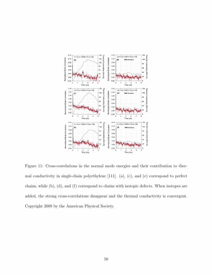
Figure 11: Cross-correlations in the normal mode energies and their contribution to ther-

mal conductivity in single-chain polyethylene [111]. (a), (c), and (e) correspond to perfect

chains, while (b), (d), and (f) correspond to chains with isotopic defects. When isotopes are

added, the strong cross-correlations disappear and the thermal conductivity is convergent.

Copyright 2009 by the American Physical Society.

50

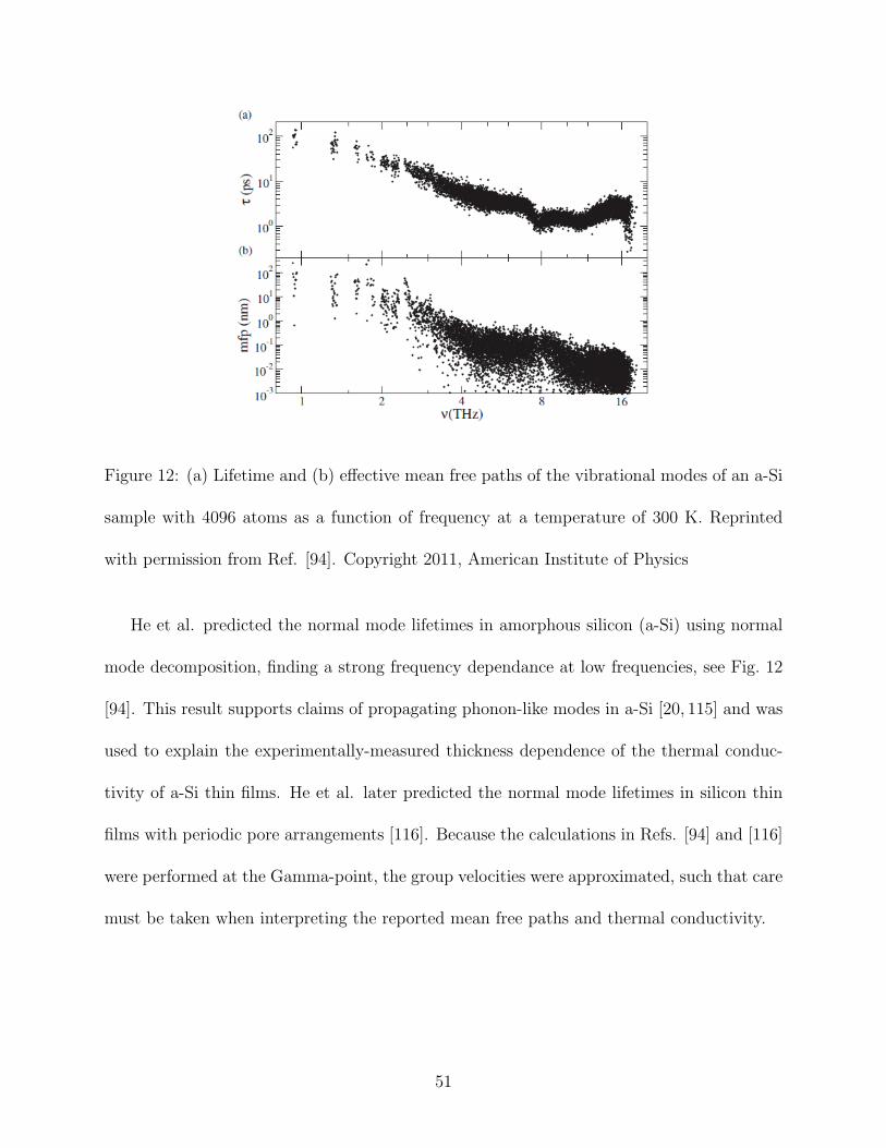
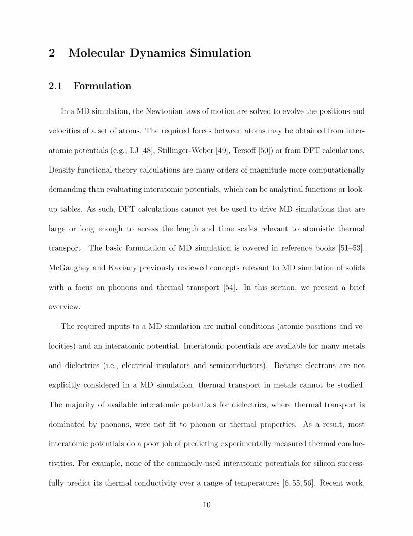
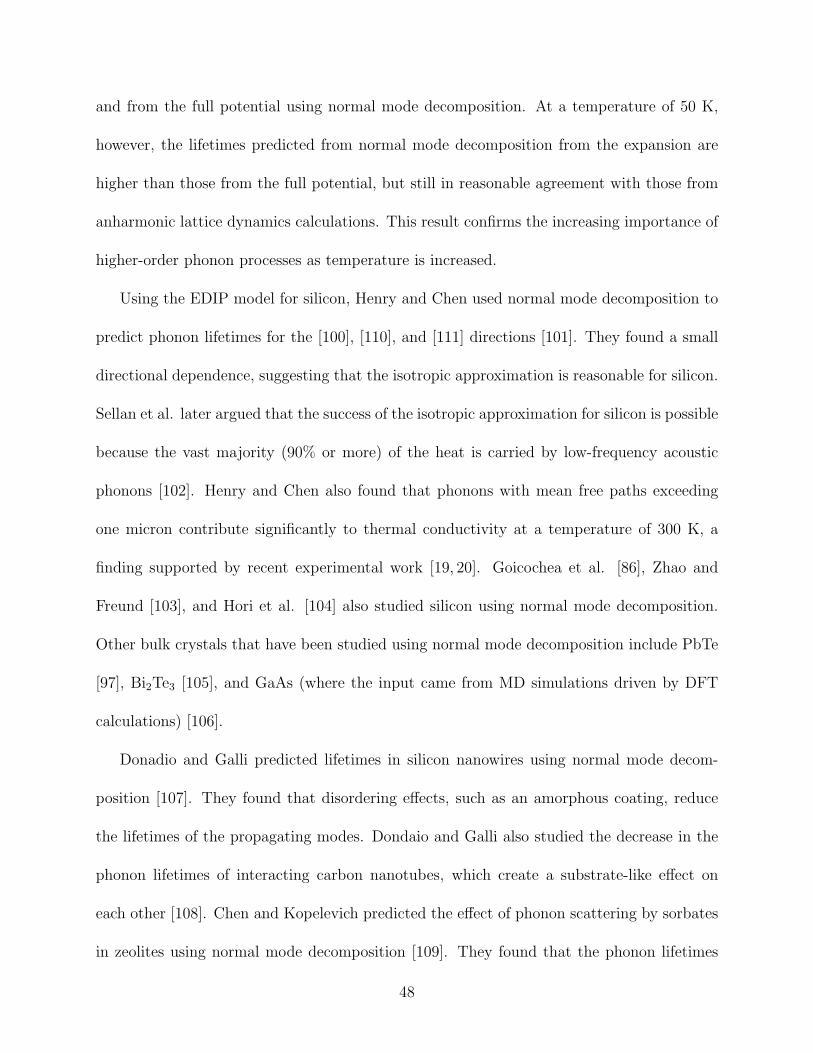
Figure 12: (a) Lifetime and (b) effective mean free paths of the vibrational modes of an a-Si

sample with 4096 atoms as a function of frequency at a temperature of 300 K. Reprinted

with permission from Ref. [94]. Copyright 2011, American Institute of Physics

He et al. predicted the normal mode lifetimes in amorphous silicon (a-Si) using normal

mode decomposition, finding a strong frequency dependance at low frequencies, see Fig. 12

[94]. This result supports claims of propagating phonon-like modes in a-Si [20, 115] and was

used to explain the experimentally-measured thickness dependence of the thermal conduc-

tivity of a-Si thin films. He et al. later predicted the normal mode lifetimes in silicon thin

films with periodic pore arrangements [116]. Because the calculations in Refs. [94] and [116]

were performed at the Gamma-point, the group velocities were approximated, such that care

must be taken when interpreting the reported mean free paths and thermal conductivity.

51

6 Summary and Outlook

In this chapter, we showed how MD simulations, lattice dynamics calculations, and nor-

mal mode decomposition can be used to predict the frequencies and lifetimes of the normal

modes of vibration in crystals, alloys, and amorphous solids. For crystals, the lifetimes

capture phonon-phonon scattering. For a dilute alloy, where the alloying atoms act as a

perturbation to the phonon modes of the associated virtual crystal, the lifetimes capture

both phonon-phonon and phonon-mass defect scattering. For an amorphous solid, the cal-

culations must be performed using the simulation cell as the unit cell (i.e., Gamma-point

analysis).

Given a set of phonon-phonon lifetimes for a crystal, the effects of other scattering mech-

anisms (e.g., point defects, grain or system boundaries) on the phonon lifetimes can be

included using the Matthiessen rule [1] or Monte Carlo approaches [72].9 The underlying

theory is typically simpler than that for phonon-phonon scattering. For example, defect

scattering is typically assumed to be an elastic process (i.e., the incoming and scattered

phonons have the same frequency), such that harmonic lattice dynamics theory can be used

to predict the associated lifetime [24, 122]. Phonon-boundary scattering is typically assumed

to be frequency-independent, so that only the system geometry is needed to specify the life-

time [1, 123]. A set of bulk phonon properties is required as input for numerical solutions to

the BTE [73, 124–126] (Chapters [Hadjiconstantinou] and [Murthy]), which can access com-

9Using bulk phonon properties to model a nanostructure is an assumption. If the nanostructure is too

small, the bulk normal modes will not be a good representation of the true normal modes. For silicon, it

has been suggested that nanostructures with limiting dimensions of 20-50 nm are required for bulk phonon

properties to be appropriate [85, 117–121]. More work is required in this direction.

52

plex nanostructure geometries and predict the time evolution of phonon populations. To

predict the thermal performance of a multi-component nanostructure or device also requires

the thermal resistances of the internal interfaces. Modeling approaches for predicting the

thermal conductance of interfaces are covered in Chapters [Fisher], [Chalopin], and [Shiomi]

[74, 127–133].

As a means to predict phonon properties, MD simulations have limitations. Notably,

(i) they are a classical (i.e., high-temperature) technique, and (ii) the majority of available

interatomic potentials do a poor job of predicting phonon properties and thermal conductiv-

ities that agree with experimental measurements. Given the success of anharmonic lattice

dynamics calculations coupled with force constants obtained from DFT calculations in pre-

dicting phonon properties and thermal conductivities, it is reasonable to ask what role MD

simulations will play in the future of phonon transport modeling.

There are good reasons to believe that MD simulations will continue to play an important

role from both quantitative and qualitative standpoints:

• Molecular dynamics simulations require no assumptions about the wave or particle

nature of a phonon, while the BTE assumes the phonons to be particles that can

scatter but not interfere. The ability to capture wave-like phonon effects is critical

in understanding the so-called “coherent” phonon effects that have been suggested to

explain experimental measurements on nanowires [134, 135], films with a periodic pore

arrangement [120, 136], and superlattices [137].

• Molecular dynamics simulations driven by interatomic potentials can contain millions

of atoms, allowing for the natural inclusion of defects and the development of a funda-

53

mental understanding of their effect on thermal transport. The large accessible system

sizes also allow for the modeling of entire nanostructures. Such large systems cannot

be accessed in anharmonic lattice dynamics-based approaches, which scale poorly with

the number of atoms in the unit cell.

• New interatomic potentials based on DFT force constants can do a good job of pre-

dicting phonon properties and thermal conductivity [10, 13, 39]. The generation of new

potentials tailored for phonon transport is an exciting and emerging field of study that

will allow for large, high-fidelity simulations.

Regarding the normal mode decomposition technique, future work should focus on its

applicability to systems that deviate from a perfect periodicity, either through defects in

crystals or in the study of amorphous phases. For amorphous phases, where the simulation

cell is the unit cell, effort is required to determine how to properly specify a group velocity,

needed to compute thermal conductivity and mean free paths. The applicability of normal

mode decomposition to periodic nanostructures such as superlattices is also an interesting

direction.

Acknowledgements

We thank Samuel C. Huberman, Ryan M. Iutzi, Eric S. Landry, Alexandre D. Massicotte,

John A. Thomas, Joseph E. Turney, Cristina H. Amon, and Massoud Kaviany for their

contributions to the development of techniques for using MD simulations to predict phonon

properties and thermal conductivity. We thank Bo Qui, Xiulin Ruan, Daniel P. Sellan,

and Junichiro Shimio for helpful discussions about spectral methods for predicting phonon

lifetimes. The writing of this chapter was supported by AFOSR award FA95501010098 and

54

a Harrington Faculty Fellowship at The University of Texas at Austin. The computational

work was supported in part by a grant of computer time from the DOD High Performance

Computing Modernization Program at the US Army Engineer Research and Development

Center.

55

References

[1] J. M. Ziman, Electrons and Phonons, Oxford, New York, 2001.

[2] M. Omini and A. Sparavigna, Thermal Conductivity of Rare Gas Crystals: The Roleof Three-Phonon Processes, Philos. Mag. B, Vol. 68, pp. 767–785, 1993.

[3] M. Omini and A. Sparavigna, Beyond the isotropic assumption in the theory of thermalconductivity, Phys. Rev. B, Vol. 53, pp. 9064–9073, 1996.

[4] M. Omini and A. Sparavigna, Thermal Conductivity of dielectric solids with diamondstructure, Nuovo Cimento D, Vol. 19, p. 1537, 1997.

[5] A. Sparavigna, Role of nonpairwise interactions on phonon thermal transport, Phys.Rev. B, Vol. 67, p. 144305, 2003.

[6] D. A. Broido, A. Ward, and N. Mingo, Lattice Thermal Conductivity of Silicon FromEmpirical Interatomic Potentials, Phys. Rev. B, Vol. 72, p. 014308, 2005.

[7] D. A. Broido, M. Maloney, G. Birner, N. Mingo, and D. Stewart, Intrinsic Lattice Ther-mal Conductivity of Semiconductors from First Principles, Appl. Phys. Lett., Vol. 91,p. 231922, 2007.

[8] L. Lindsay, D. A. Broido, and N. Mingo, Lattice thermal conductivity of single-walledcarbon nanotubes: Beyond the relaxation time approximation and phonon-phononscattering selection rules, Phys. Rev. B, Vol. 80, p. 125407, 2009.

[9] A. Ward and D. A. Broido, Intrinsic phonon relaxation times from first-principlesstudies of the thermal conductivities of Si and Ge, Phys. Rev. B, Vol. 81, p. 085205,2010.

[10] L. Lindsay and D. A. Broido, Optimized Tersoff and Brenner empirical potential pa-rameters for lattice dynamics and phonon thermal transport in carbon nanotubes andgraphene, Phys. Rev. B, Vol. 81, p. 205441, 2010.

[11] A. Chernatynskiy and S. R. Phillpot, Evaluation of computational techniques for solv-ing the Boltzmann transport equation for lattice thermal conductivity calculations,Phys. Rev. B, Vol. 82, p. 134301, 2010.

[12] A. Chernatynskiy, J. E. Turney, A. J. H. McGaughey, C. H. Amon, and S. R. Phillpot,Phonon-mediated thermal conductivity in ionic solids by lattice-dynamics based meth-ods, J. Am. Ceram. Soc., Vol. 94, pp. 3523–3531, 2011.

[13] D. Singh, J. Y. Murthy, and T. S. Fisher, Spectral phonon conduction and dominantscattering pathways in graphene, J. Appl. Phys., Vol. 110, 094312, 2011.

[14] A. A. Maradudin and A. E. Fein, Scattering of Neutrons by an Anharmonic Crystal,Phys. Rev., Vol. 128, pp. 2589–2608, 1962.

56

[15] R. Stedman, L. Almqvist, and G. Nilsson, Phonon-Frequency Distributions and HeatCapacities of Aluminum and Lead, Phys. Rev., Vol. 162, pp. 549–557, 1967.

[16] T. R. Hart, R. L. Aggarwal, and B. Lax, Temperature Dependence of Raman Scatteringin Silicon, Phys. Rev. B, Vol. 1, pp. 638–642, 1970.

[17] Y. K. Koh and D. G. Cahill, Frequency dependence of the thermal conductivity ofsemiconductor alloys, Phys. Rev. B, Vol. 76, p. 075207, 2007.

[18] M. E. Siemens, Q. Li, R. Yang, K. A. Nelson, E. H. Anderson, M. M. Murnane, andH. C. Kapteyn, Quasi-ballistic thermal transport from nanoscale interfaces observedusing ultrafast coherent soft X-ray beams, Nat. Mater., Vol. 9, pp. 26–30, 2010.

[19] A. J. Minnich, J. A. Johnson, A. J. Schmidt, K. Esfarjani, M. S. Dresselhaus, K. A. Nel-son, and G. Chen, Thermal Conductivity Spectroscopy Technique to Measure PhononMean Free Paths, Phys. Rev. Lett., Vol. 107, p. 095901, 2011.

[20] K. Regner, D. P. Sellan, Z. Su, C. H. Amon, A. J. H. McGaughey, and J. A. Malen,to appear in Nat. Commun..

[21] J. A. Johnson, A. A. Maznev, M. T. Bulsara, E. A. Fitzgerald, T. C. Harman,S. Calawa, C. J. Vineis, G. Turner, and K. A. Nelson, Phase-controlled, heterodynelaser-induced transient grating measurements of thermal transport properties in opaquematerial, J. Appl. Phys., Vol. 111, 023503, 2012.

[22] J. A. Johnson, A. A. Maznev, J. Cuffe, J. K. Eliason, A. J. Minnich, T. Kehoe,C. M. S. Torres, G. Chen, and K. A. Nelson, Direct Measurement of Room-TemperatureNondiffusive Thermal Transport Over Micron Distances in a Silicon Membrane, Phys.Rev. Lett., Vol. 110, p. 025901, 2013.

[23] C. Dames and G. Chen, Thermal conductivity of nanostructured thermoelectric mate-rials, In D. M. Rowe, Ed., Thermoelectrics Handbook: Macro to Nano, Baton Rouge,FL: Taylor & Francis, pp. 42–1 – 42–11, 2005.

[24] P. G. Klemens, The scattering of low-frequency lattice waves by static imperfections,P. Roy. Soc. A, Vol. 68, pp. 1113–1128, 1955.

[25] J. Callaway, Model for lattice thermal conductivity at low temperatures, Phys. Rev.,Vol. 113, p. 1046, 1959.

[26] M. G. Holland, Analysis of lattice thermal conductivity, Phys. Rev., Vol. 132, p. 2461,1963.

[27] G. A. Slack, Nonmetallic crystals with high thermal conductivity, J. Phys. Chem.Solids, Vol. 34, pp. 321–335, 1973.

[28] J. D. Chung, A. J. H. McGaughey, and M. Kaviany, Role of phonon dispersion inlattice thermal conductivity analysis, J.Heat Transf., Vol. 126, pp. 376–380, 2004.

57

[29] V. L. Gurevich, Transport in Phonon Systems, North-Holland, Amsterdam, 1986.

[30] K. Esfarjani and H. T. Stokes, Method to extract anharmonic force constants fromfirst principles calculations, Phys. Rev. B, Vol. 77, p. 144112, 2008.

[31] W. Li, L. Lindsay, D. A. Broido, D. A. Stewart, and N. Mingo, Thermal conductivityof bulk and nanowire Mg2SixSn1−x alloys from first principles, Phys. Rev. B, Vol. 86,p. 174307, 2012.

[32] D. C. Wallace, Thermodynamics of Crystals, Cambridge University Press, Cambridge,UK, 1972.

[33] A. A. Maradudin, In G. K. Horton and A. A. Maradudin, Eds., Dynamical Propertiesof Solids, Volume 1. Crystalline Solids, Fundamentals, New York: Elsevier, pp. 1–82,1974.

[34] M. T. Dove, Introduction to Lattice Dynamics, Cambridge, Cambridge, 1993.

[35] A. J. H. McGaughey, M. I. Hussein, E. S. Landry, M. Kaviany, and G. M. Hulbert,Phonon Band Structure and Thermal Transport Correlation in a Layered DiatomicCrystal, Phys. Rev. B, Vol. 74, p. 104304, 2006.

[36] A. J. C. Ladd, B. Moran, and W. G. Hoover, Lattice thermal conductivity: A compar-ison of molecular dynamics and anharmonic lattice dynamics, Phys. Rev. B, Vol. 34,pp. 5058–5064, 1986.

[37] J. E. Turney, E. S. Landry, A. J. H. McGaughey, and C. H. Amon, Predicting phononproperties and thermal conductivity from anharmonic lattice dynamics calculationsand molecular dynamics simulations, Phys. Rev. B, Vol. 79, p. 064301, 2009.

[38] A. Ward, D. A. Broido, D. A. Stewart, and G. Deinzer, Ab initio theory of the latticethermal conductivity in diamond, Phys. Rev. B, Vol. 80, p. 125203, 2009.

[39] K. Esfarjani, G. Chen, and H. T. Stokes, Heat transport in silicon from first-principlescalculations, Phys. Rev. B, Vol. 84, p. 085204, 2011.

[40] J. Garg, N. Bonini, B. Kozinsky, and N. Marzari, Role of Disorder and Anharmonicityin the Thermal Conductivity of Silicon-Germanium Alloys: A First-Principles Study,Phys. Rev. Letters, Vol. 106, p. 045901, 2011.

[41] J. Shiomi, K. Esfarjani, and G. Chen, Thermal conductivity of half-Heusler compoundsfrom first-principles calculations, Phys. Rev. B, Vol. 84, p. 104302, 2011.

[42] L. Lindsay, D. A. Broido, and T. L. Reinecke, Thermal Conductivity and Large IsotopeEffect in GaN from First Principles, Phys. Rev. Lett., Vol. 109, p. 095901, 2012.

[43] Z. Tian, J. Garg, K. Esfarjani, T. Shiga, J. Shiomi, and G. Chen, Phonon conduction inPbSe, PbTe, and PbTe1−xSex from first-principles calculations, Phys. Rev. B, Vol. 85,p. 184303, 2012.

58

[44] T. Shiga, J. Shiomi, J. Ma, O. Delaire, T. Radzynski, A. Lusakowski, K. Esfarjani,and G. Chen, Microscopic mechanism of low thermal conductivity in lead telluride,Phys. Rev. B, Vol. 85, p. 155203, 2012.

[45] T. Luo, J. Garg, J. Shiomi, K. Esfarjani, and G. Chen, Gallium arsenide thermalconductivity and optical phonon relaxation times from first-principles calculations,Europhys. Lett., Vol. 101, p. 16001, 2013.

[46] A. J. H. McGaughey and M. Kaviany, Quantitative Validation of the Boltzmann Trans-port Equation Phonon Thermal Conductivity Model Under the Single-mode Relax-ation Time Approximation, Phys. Rev. B, Vol. 69, p. 094303, 2004.

[47] J. M. Larkin, J. E. Turney, A. D. Massicotte, C. H. Amon, and A. J. H. McGaughey,to appear in J. Comput. Theor. Nanos.

[48] N. W. Ashcroft and N. D. Mermin, Solid State Physics, Saunders, Fort Worth, 1976.

[49] F. H. Stillinger and T. A. Weber, Computer Simulation of Local Order in CondensedPhases of Silicon, Phys. Rev. B, Vol. 31, pp. 5262–5271, 1985.

[50] J. Tersoff, New empirical approach for the structure and energy of covalent systems,Phys. Rev. B, Vol. 37, pp. 6991–7000, 1988.

[51] M. P. Allen and D. J. Tildesley, Computer Simulation of Liquids, Clarendon Press,Oxford, 1987.

[52] D. Frenkel and B. Smit, Understanding Molecular Simulation: From Algorithms toApplications, Academic Press, San Diego, 2001.

[53] D. C. Rapaport, The Art of Molecular Dynamics Simulation, Cambridge UniversityPress, Cambridge, 2004.

[54] A. J. H. McGaughey and M. Kaviany, Phonon transport in molecular dynamics sim-ulations: Formulation and thermal conductivity prediction, In G. A. Greene, Y. I.Cho, J. P. Hartnett, and A. Bar-Cohen, Eds., Advances in Heat Transfer, Volume 39,London: Academic Press, pp. 169–255, 2006.

[55] P. K. Schelling, S. R. Phillpot, and P. Keblinski, Comparison of atomic-level simulationmethods for computing thermal conductivity, Phys. Rev. B, Vol. 65, p. 144306, 2002.

[56] P. C. Howell, Comparison of molecular dynamics methods and interatomic potentialsfor calculating the thermal conductivity of silicon, J. Chem. Phys., Vol. 137, 224111,2012.

[57] P. K. Schelling, S. R. Phillpot, and P. Keblinski, Phonon wave-packet dynamics atsemiconductor interfaces by molecular-dynamics simulation, Appl. Phys. Lett., Vol. 80,pp. 2484–2486, 2002.

[58] C. H. Baker, D. A. Jordan, and P. M. Norris, Application of the wavelet transform tonanoscale thermal transport, Phys. Rev. B, Vol. 86, p. 104306, 2012.

59

[59] D. A. McQuarrie, Statistical Mechanics, University Science Books, Sausalito, 2000.

[60] J. E. Turney, A. J. H. McGaughey, and C. H. Amon, Assessing the applicabilityof quantum corrections to classical thermal conductivity predictions, Phys. Rev. B,Vol. 79, p. 224305, 2009.

[61] E. S. Landry, M. I. Hussein, and A. J. H. McGaughey, Complex superlattice unit celldesigns for reduced thermal conductivity, Phys. Rev. B, Vol. 77, p. 184302, 2008.

[62] X. W. Zhou, S. Aubry, R. E. Jones, A. Greenstein, and P. K. Schelling, Towards moreaccurate molecular dynamics calculation of thermal conductivity: Case study of GaNbulk crystals, Phys. Rev. B, Vol. 79, p. 115201, 2009.

[63] J. Chen, G. Zhang, and B. Li, How to improve the accuracy of equilibrium moleculardynamics for computation of thermal conductivity?, Phys. Lett. A, Vol. 374, pp. 2392– 2396, 2010.

[64] D. P. Sellan, E. S. Landry, J. E. Turney, A. J. H. McGaughey, and C. H. Amon, Sizeeffects in molecular dynamics thermal conductivity predictions, Phys. Rev. B, Vol. 81,p. 214305, 2010.

[65] P. C. Howell, Thermal Conductivity Calculation with the Molecular Dynamics DirectMethod I: More Robust Simulations of Solid Materials, J. Comput. Theor. Nanos.,Vol. 8, pp. 2129–2143, 2011.

[66] P. C. Howell, Thermal Conductivity Calculation with the Molecular Dynamics DirectMethod II: Improving the Computational Efficiency, J. Comput.Theor. Nanos., Vol. 8,pp. 2144–2154, 2011.

[67] Y. He, I. Savic, D. Donadio, and G. Galli, Lattice thermal conductivity of semicon-ducting bulk materials: atomistic simulations, Phys. Chem. Chem. Phys., Vol. 14, pp.16209–16222, 2012.

[68] R. E. Jones and K. K. Mandadapu, Adaptive Green-Kubo estimates of transport coef-ficients from molecular dynamics based on robust error analysis, J.Chem. Phys., Vol.136, 154102, 2012.

[69] A. J. H. McGaughey and M. Kaviany, Thermal conductivity decomposition and anal-ysis using molecular dynamics simulations. Part I. Lennard-Jones argon, InternationalJournal of Heat and Mass Transfer, Vol. 47, pp. 1783–1798, 2004.

[70] A. J. H. McGaughey and M. Kaviany, Thermal conductivity decomposition and anal-ysis using molecular dynamics simulations. Part II. Complex Silica Structures, Int. J.Heat Mass Tran., Vol. 47, pp. 1799–1816, 2004.

[71] L. Hu, W. J. Evans, and P. Keblinski, One-dimensional phonon effects in direct molec-ular dynamics method for thermal conductivity determination, J. Appl. Phys., Vol.110, 113511, 2011.

60

[72] A. J. H. McGaughey and A. Jain, Nanostructure thermal conductivity prediction byMonte Carlo sampling of phonon free paths, Appl. Phys. Lett., Vol. 100, p. 061911,2012.

[73] J.-P. M. Peraud and N. G. Hadjiconstantinou, An alternative approach to efficientsimulation of micro/nanoscale phonon transport, Appl. Phys. Lett., Vol. 101, 153114,2012.

[74] J.-S. Wang, J. Wang, and J. T. Li, Quantum Thermal Transport in Nanostructures,Eur. Phys. J. B, Vol. 62, pp. 381–404, 2008.

[75] Larkin, J. M., Vibrational Properties of Disordered System, PhD Thesis, CarnegieMellon University, 2012.

[76] W. Rudin, Real and Complex Analysis, McGraw-Hill, New York, 1987.

[77] J. D. Gale, GULP: A computer program for the symmetry-adapted simulation of solids,J. Chem. Soc. Faraday T., Vol. 93, pp. 629–637, 1997.

[78] J. D. Gale and A. L. Rohl, The General Utility Lattice Program (GULP), Mol. Sim-ulat., Vol. 29, pp. 291–341, 2003.

[79] J. D. Gale, GULP: Capabilities and prospects, Z. Kristallogr., Vol. 220, pp. 552–554,2005.

[80] S. Plimpton, Fast Parallel Algorithms for Short-Range Molecular Dynamics, J. Com-put. Phys., Vol. 117, pp. 1–19, 1995.

[81] S. Plimpton and A. P. Thompson, Computational Aspects of Many-body Potentials,MRS Bull., Vol. 37, pp. 513–521, 2012.

[82] P. F. Dubois, K. Hinsen, and J. Hugunin, Numerical Python, Comput. Phys., Vol. 10,1996.

[83] McGaughey, A. J. H.,Phonon transport in molecular dynamics simulations: Formu-lation and thermal conductivity prediction, PhD Thesis, University of Michigan, AnnArbor, 2004.

[84] S. N. Taraskin and S. R. Elliott, Determination of the Ioffe-Regel limit for vibrationalexcitations in disordered materials, Philos. Mag. B, Vol. 79, pp. 1747–1754, 1999.

[85] J. E. Turney, A. J. H. McGaughey, and C. H. Amon, In-plane phonon transport inthin films, J. Appl. Phys., Vol. 107, 024317, 2010.

[86] J. V. Goicochea, M. Madrid, and C. H. Amon, Thermal Properties for Bulk SiliconBased on the Determination of Relaxation Times Using Molecular Dynamics, J. HeatTransf., Vol. 132, p. 012401, 2010.

[87] A. Skye and P. K. Schelling, Thermal resistivity of Si–Ge alloys by molecular-dynamicssimulation, J. Appl. Phys., Vol. 103, 113524, 2008.

61

[88] D. G. Cahill, F. Watanabe, A. Rockett, and C. B. Vining, Thermal conductivity ofepitaxial layers of dilute SiGe alloys, Phys. Rev. B, Vol. 71, p. 235202, 2005.

[89] B. Abeles, Lattice Thermal Conductivity of Disordered Semiconductor Alloys at HighTemperatures, Phys. Rev., Vol. 131, pp. 1906–1911, 1963.

[90] P. B. Allen, J. L. Feldman, J. Fabian, and F. Wooten, Diffusons, locons, and propagons:character of atomic vibrations in amorphous Si, Philos. Mag. B, Vol. 79, pp. 1715–1731,1999.

[91] P. B. Allen and J. L. Feldman, Thermal conductivity of disordered harmonic solids,Phys. Rev. B, Vol. 48, pp. 12581–12588, 1993.

[92] J. L. Feldman, M. D. Kluge, P. B. Allen, and F. Wooten, Thermal conductivity andlocalization in glasses: Numerical study of a model of amorphous silicon, Phys. Rev.B, Vol. 48, pp. 12589–12602, 1993.

[93] S. Shenogin, A. Bodapati, P. Keblinski, and A. J. H. McGaughey, Predicting thethermal conductivity of inorganic and polymeric glasses: The role of anharmonicity,J. Appl. Phys., Vol. 105, 034906, 2009.

[94] Y. He, D. Donadio, and G. Galli, Heat transport in amorphous silicon: Interplaybetween morphology and disorder, Appl. Phys. Lett., Vol. 98, 144101, 2011.

[95] N. de Koker, Thermal Conductivity of MgO Periclase from Equilibrium First PrinciplesMolecular Dynamics, Phys. Rev. Lett., Vol. 103, 125902, 2009.

[96] J. A. Thomas, J. E. Turney, R. M. Iutzi, C. H. Amon, and A. J. H. McGaughey,Predicting phonon dispersion relations and lifetimes from the spectral energy density,Phys. Rev. B, Vol. 81, p. 081411, 2010.

[97] B. Qiu, H. Bao, G. Zhang, Y. Wu, and X. Ruan, Molecular dynamics simulations oflattice thermal conductivity and spectral phonon mean free path of PbTe: Bulk andnanostructures, Comp. Mater. Sci., Vol. 53, pp. 278 – 285, 2012.

[98] Z.-Y. Ong, E. Pop, and J. Shiomi, Reduction of phonon lifetimes and thermal con-ductivity of a carbon nanotube on amorphous silica, Phys. Rev. B, Vol. 84, p. 165418,2011.

[99] L. Chen and S. Kumar, Thermal transport in graphene supported on copper, J. Appl.Phys., Vol. 112, p. 043502, 2012.

[100] S. Maruyama, A Molecular Dynamics Simulation of Heat Conduction of a FiniteLength Single-Walled Carbon Nanotube, Microscale Therm. Eng., Vol. 7, pp. 41–50,2003.

[101] A. S. Henry and G. Chen, Spectral Phonon Transport Properties of Silicon Based onMolecular Dynamics Simulations and Lattice Dynamics, J. Comput. Theor. Nanos.,Vol. 5, pp. 1–12, 2008.

62

[102] D. P. Sellan, J. E. Turney, A. J. H. McGaughey, and C. H. Amon, Cross-plane phonontransport in thin films, J. Appl. Phys., Vol. 108, p. 113524, 2010.

[103] H. Zhao and J. B. Freund, Full-spectrum phonon relaxation times in crystalline Sifrom molecular dynamics simulations, J. Appl. Phys., Vol. 104, 033514, 2008.

[104] T. Hori, T. Shiga, S. Maruyama, and J. Shiomi, Mode-Dependent Phonon TransportAnalysis of Silicon Crystal by Molecular Dynamics Method, T. Jpn. Soc. Mech. Eng.,Vol. 78, pp. 328–337, 2012.

[105] Y. Wang, B. Qiu, A. J. H. McGaughey, X. Ruan, and X. Xu, to appear in J. HeatTransf..

[106] H. Bao, B. Qiu, Y. Zhang, and X. Ruan, A first-principles molecular dynamics approachfor predicting optical phonon lifetimes and far-infrared reflectance of polar materials,J. Quant. Spectrosc. Ra., Vol. 113, pp. 1683 – 1688, 2012.

[107] D. Donadio and G. Galli, Atomistic Simulations of Heat Transport in SiliconNanowires, Phys. Rev. Lett., Vol. 102, p. 195901, 2009.

[108] D. Donadio and G. Galli, Thermal Conductivity of Isolated and Interacting CarbonNanotubes: Comparing Results from Molecular Dynamics and the Boltzmann Trans-port Equation, Phys. Rev. Lett., Vol. 99, p. 255502, 2007.

[109] C.-Y. Chen and D. I. Kopelevich, Phonon interactions in zeolites mediated by anhar-monicity and adsorbed molecules, Mol. Simulat., Vol. 34, pp. 155–167, 2008.

[110] A. Henry and G. Chen, High Thermal Conductivity of Single Polyethylene ChainsUsing Molecular Dynamics Simulations, Phys. Rev. Lett., Vol. 101, 235502, 2008.

[111] A. Henry and G. Chen, Anomalous heat conduction in polyethylene chains: Theoryand molecular dynamics simulations, Phys. Rev. B, Vol. 79, 144305, 2009.

[112] T. Sun, X. Shen, and P. B. Allen, Phonon quasiparticles and anharmonic perturbationtheory tested by molecular dynamics on a model system, Phys. Rev. B, Vol. 82, p.224304, 2010.

[113] T. Sun and P. B. Allen, Lattice thermal conductivity: Computations and theory ofthe high-temperature breakdown of the phonon-gas model, Phys. Rev. B, Vol. 82, p.224305, 2010.

[114] A. Henry and G. Chen, Explicit treatment of hydrogen atoms in thermal simulationsof polyetylene, Nanosc. Microsc Therm., Vol. 13, pp. 99–108, 2009.

[115] D. G. Cahill, M. Katiyar, and J. R. Abelson, Thermal conductivity of α-Si:H thinfilms, Phys. Rev. B, Vol. 50, pp. 6077–6081, 1994.

[116] Y. He, D. Donadio, J.-H. Lee, J. C. Grossman, and G. Galli, Thermal Transport inNanoporous Silicon: Interplay between Disorder at Mesoscopic and Atomic Scales,ACS Nano, Vol. 5, pp. 1839–1844, 2011.

63

[117] A. Balandin and K. L. Wang, Significant decrease of the lattice thermal conductivitydue to phonon confinement in a free-standing semiconductor quantum well, Phys. Rev.B, Vol. 58, pp. 1544–1549, 1998.

[118] N. Mingo, Calculation of Si nanowire thermal conductivity using complete phonondispersion relations, Phys. Rev. B, Vol. 68, p. 113308, 2003.

[119] P. Martin, Z. Aksamija, E. Pop, and U. Ravaioli, Impact of Phonon-Surface RoughnessScattering on Thermal Conductivity of Thin Si Nanowires, Phys. Rev. Lett., Vol. 102,p. 125503, 2009.

[120] J.-K. Yu, S. Mitrovic, D. Tham, J. Varghese, and J. R. Heath, Reduction of thermalconductivity in phononic nanomesh structures, Nat. Nanotechnol., Vol. 5, pp. 718–721,2010.

[121] A. Jain, Y.-J. Yu, and A. J. H. McGaughey, submitted.

[122] S. Tamura, Isotope scattering of dispersive phonons in Ge, Phys. Rev. B, Vol. 27, pp.858–866, 1983.

[123] A. J. H. McGaughey, E. S. Landry, D. P. Sellan, and C. H. Amon, Size-dependentmodel for thin film and nanowire thermal conductivity, Appl. Phys. Lett., Vol. 99, p.131904, 2011.

[124] S. Mazumder and A. Majumdar, Monte Carlo Study of Phonon Transport in Solid ThinFilms Including Dispersion and Polarization, J. Heat Transf., Vol. 123, pp. 749–759,2001.

[125] J.-P. M. Peraud and N. G. Hadjiconstantinou, Efficient simulation of multidimen-sional phonon transport using energy-based variance-reduced Monte Carlo formula-tions, Phys. Rev. B, Vol. 84, p. 205331, 2011.

[126] A. Nabovati, D. P. Sellan, and C. H. Amon, On the lattice Boltzmann method forphonon transport, J. Comput. Phys., Vol. 230, pp. 5864 – 5876, 2011.

[127] P. K. Schelling, S. R. Phillpot, and P. Keblinski, Kapitza conductance and phononscattering at grain boundaries by simulation, J. Appl. Phys., Vol. 95, pp. 6082–6091,2004.

[128] H. Zhao and J. B. Freund, Lattice-dynamical Calculation of Phonon Scattering at IdealSi-Ge Interfaces, J. Appl. Phys., Vol. 97, p. 024903, 2005.

[129] R. J. Stevens, L. V. Zhigilei, and P. M. Norris, Effects of temperature and disorderon thermal boundary conductance at solidsolid interfaces: Nonequilibrium moleculardynamics simulations, Int. J. Heat Mass Tran., Vol. 50, pp. 3977–3989, 2007.

[130] E. S. Landry and A. J. H. McGaughey, Thermal boundary resistance predictions frommolecular dynamics simulations and theoretical calculations, Phys. Rev. B, Vol. 80, p.165304, 2009.

64

[131] Y. Chalopin, K. Esfarjani, A. Henry, S. Volz, and G. Chen, Thermal interface conduc-tance in Si/Ge superlattices by equilibrium molecular dynamics, Phys. Rev. B, Vol. 85,p. 195302, 2012.

[132] S. Merabia and K. Termentzidis, Thermal conductance at the interface between crystalsusing equilibrium and nonequilibrium molecular dynamics, Phys. Rev. B, Vol. 86, p.094303, 2012.

[133] Z. Tian, K. Esfarjani, and G. Chen, Enhancing phonon transmission across a Si/Ge in-terface by atomic roughness: First-principles study with the Green’s function method,Phys. Rev. B, Vol. 86, p. 235304, 2012.

[134] A. I. Hochbaum, R. Chen, R. D. Delgado, W. Liang, E. C. Garnett, M. Najarian,A. Majumdar, and P. Yang, Enhanced thermoelectric performance of rough siliconnanowires, Nature, Vol. 451, pp. 163–167, 2008.

[135] A. I. Boukai, Y. Bunimovich, J. Tahi-Kheli, J.-K. Yu, W. A. G. Goddard, and J. R.Heath, Silicon nanowires as efficient thermoelectric materials, Nature, Vol. 451, pp.168–171, 2008.

[136] J. Tang, H.-T. Wang, D. H. Lee, M. Fardy, Z. Huo, T. P. Russell, and P. Yang, HoleySilicon as an Efficient Thermoelectric Material, Nano Lett., Vol. 10, pp. 4279–4283,2010.

[137] M. N. Luckyanova, J. Garg, K. Esfarjani, A. Jandl, M. T. Bulsara, A. J. Schmidt,A. J. Minnich, S. Chen, M. S. Dresselhaus, Z. Ren, E. A. Fitzgerald, and G. Chen,Coherent Phonon Heat Conduction in Superlattices, Science, Vol. 338, pp. 936–939,2012.

65