Predicting stock price movements from past returns: the - Faculty

Journal of Financial Economics 71 (2004) 541–579

Predicting stock price movements frompast returns: the role of consistency and

tax-loss selling$

Mark Grinblatta, Tobias J. Moskowitzb,*aThe Anderson School at UCLA, Yale ICF, and NBER, Los Angeles, CA 90095, USA

bGraduate School of Business, University of Chicago and NBER, 1101 E. 58th st., Chicago, IL 60637, USA

Received 10 May 2000; accepted 29 January 2003

Abstract

The consistency of positive past returns and tax-loss selling significantly affects the relation

between past returns and the cross-section of expected returns. Analysis of these additional

effects across stock characteristics, seasons, and tax regimes provides clues about the sources

of temporal relations in stock returns, pointing to potential explanations for this relation. A

parsimonious trading rule generates surprisingly large economic returns despite controls for

confounding sources of return premia, microstructure effects, and data snooping biases.

r 2003 Elsevier B.V. All rights reserved.

JEL classification: G11; G12; G14

Keywords: Market efficiency; Return autocorrelation; Momentum; Tax-loss trading

ARTICLE IN PRESS

$We thank John Cochrane, Joshua Coval, Eugene Fama, Bill Gebhardt, Bing Han, Owen Lamont, Ed

Maydew, Tuomo Vuolteenaho, an anonymous referee, and seminar participants at the University of

Chicago, Cornell University, Virginia Tech, New York University, Washington State University, and the

2000 AFA meetings in Boston for valuable comments and suggestions. We also wish to thank Bing Han

for outstanding research assistance and Avanidhar Subrahmanyam for providing data on institutional

ownership. Grinblatt was a visiting fellow at Yale University’s School of Management while earlier drafts

of this paper were completed. He is grateful to the UCLA Academic Senate and to Yale University for the

support they provided. Moskowitz thanks the Center for Research in Security Prices, the Dimensional

Fund Advisors Research Fund, and the James S. Kemper Faculty Research Fund at the University of

Chicago for financial support.

*Corresponding author. Tel.: +1-773-834-2757; fax: +1-773-702-0458.

E-mail address: [email protected] (T.J. Moskowitz).

0304-405X/$ - see front matter r 2003 Elsevier B.V. All rights reserved.

doi:10.1016/S0304-405X(03)00176-4

1. Introduction

Within the last two decades, researchers have discovered that past returns containinformation about expected returns. Both short- (less than one month) and long-term (three-to-five year) past returns are inversely related to future average returns,while intermediate horizon past returns (three to 12 months) are positively related tofuture average returns. Classic papers include Jegadeesh (1990), DeBondt and Thaler(1985), and Jegadeesh and Titman (1993).1

A variety of explanations are offered for these relations. They range from dataissues, such as microstructure and data snooping biases (Boudoukh et al., 1994;Conrad and Kaul, 1989; Lo and MacKinlay, 1988), to rational risk-basedexplanations (Conrad and Kaul, 1998; Berk et al., 1999; Chordia and Shivakumar,2002; Bansal et al., 2002), to irrational behavioral stories (DeBondt and Thaler,1985, 1987; Jegadeesh and Titman, 1993; Daniel et al., 1998; Barberis et al., 1998;Hong and Stein, 1999; Hong et al., 2000; Lee and Swaminathan, 2000; Grinblatt andHan, 2002). Despite the ability of creative theorists and talented critics of empiricalwork to explain the sign of an observed temporal return relation, the field of financefinds it difficult to reconcile theory with the exceptional profits generated by tradingstrategies that exploit these patterns. Moreover, only recently have theories evolved,and these generally of the behavioral variety, that explain these multi-horizon andopposite-signed temporal relations synthetically. Yet little empirical work analyzesthese patterns simultaneously and, as we will show, there are additional complexitiesto these relations that appear inconsistent with most existing explanations.

Before proposing novel theories for these effects, we need to better understandwhether past returns predict future returns because they are a proxy for a morefundamental variable that predicts returns. In this regard, we analyze the consistencyand sign of the past return (over multiple past return horizons), as well as the degreeto which tax-motivated trading generates these effects.

A key finding that comes out of this analysis is that winner consistency isimportant. Achieving a high past return with a series of steady positive monthsappears to generate a larger expected return than a high past return achievedwith just a few extraordinary months. This is a finding that is predicted bytheories advanced in other papers. For instance, Grinblatt and Han (2002) arguethat the disposition effect can generate such results. Watkins (2002) argues thatinformation diffusion explains a consistency in stock returns. Consistency can alsoproxy for the inverse of volatility and this may affect average returns as a proxy forrisk.

In addition, we highlight the importance of seasonalities associated with pastreturns and the degree to which tax-loss trading plays a role in past returnpredictability. If tax-loss trading tends to mask or reverse the fundamental effects

ARTICLE IN PRESS

1DeBondt and Thaler (1987), Lo and MacKinlay (1988), Conrad and Kaul (1989), Lehman (1990),

Boudoukh et al. (1994), Rouwenhorst (1998), Moskowitz and Grinblatt (1999), Hong et al. (2000),

Grundy and Martin (2001), and Lee and Swaminathan (2000) all show autocorrelation in stock returns at

various horizons.

M. Grinblatt, T.J. Moskowitz / Journal of Financial Economics 71 (2004) 541–579542

that drive temporal return relations at certain times of the year, it would not bepossible to uncover them without isolating these effects by season. For example, wefind that for our sample period, the profitability of the three-year reversal strategy islargely confined to January. This suggests that a link between long-term reversalsand intermediate-term momentum is tenuous because the latter effect does notexhibit this seasonality. We also find that returns are strongly negative in Decemberfor losing firms, pointing to tax-loss trading as the driver of a good portion of theprofitability of momentum strategies as well as strategies that take advantage of theturn-of-the-year effect.

A host of papers analyze the January effect, including Dyl (1977), Roll (1983),Keim (1983, 1989), Reinganum (1983), Berges et al. (1984), Chan (1986),Lakonishok and Smidt (1988), Reinganum and Shapiro (1987), Dyl and Maberly(1992), and Poterba and Weisbenner (2001). Many of these papers allude to tax-losstrading as a possible source of the effect. Of course, as Constantinides (1984) shows,there should be no increase in tax-loss selling at the end of the year when short- andlong-term gains are treated equally and there are no transactions costs. However, it iscommon folk wisdom that investors pay attention to the tax implications of theirportfolios at the end of the year. Grinblatt and Keloharju (2001, 2003) use thisexplanation for Finnish investors, for instance. By inferring buying and sellingpressure from quoted daily spreads, Hvidkjaer (2001) shows year-end sellingpressure in firms that have done poorly over the prior year and subsequent year-endbuying pressure in these firms after the turn of the year. His patterns of tradingmirror our seasonal return patterns.

We argue that tax avoidance behavior, as opposed to other explanations (e.g.,window dressing), drives much of the relation between past returns and expectedreturns in December and January. This is because the seasonal differences in thecharacterization of the cross-section of expected returns mirror our analysis of howtax-code changes affect the characterization of the cross-section of expected returns.When effective capital gains tax rates are expected to decrease (providing anincentive to accelerate the realization of losses), increased selling pressure on losingstocks improves the profitability of momentum strategies, but makes contrarianstrategies relatively less profitable. Similarly, when expected tax-code changes favorcapital loss deferral, the opposite occurs. In such a case, contrarian strategies becomerelatively more profitable and the profits from momentum strategies decline. Weshow that value-weighted strategies developed from the past one-year and three-yearpatterns exhibit diminished profitability outside of January and December in low taxyears. Existing explanations for temporal return relations, both behavioral andrational, do not predict that these effects would diminish in low tax years, or vary instrength by the season of a given year, suggesting that they cannot solely explain whypast return predictability exists.

We also analyze which types of stocks lend themselves to the most profitabletechnical trading strategies. The profitability of our trading strategies varies greatlydepending on firm size, institutional ownership, and turnover despite controls forsize, book-to-market, and industry as sources of return premia. The seasonalvariation also differs across these sectors of the stock market. The sector-based

ARTICLE IN PRESSM. Grinblatt, T.J. Moskowitz / Journal of Financial Economics 71 (2004) 541–579 543

analysis helps in assessing extant theories advanced to explain why these temporalrelations exist. For instance, small, high turnover stocks with low institutionalownership exhibit more pronounced past return and seasonal effects. This furtherpoints to tax-loss selling, as opposed to window dressing, being associated with thesepatterns.

Finally, our approach in analyzing the importance of these complex patterns ofreturns is based on a parsimonious stock ranking system derived from simple Fama-MacBeth cross-sectional regressions. We analyze the simultaneous effect of anumber of past return-related variables on the future returns of hedged positions inindividual stocks, which have their size, book-to-market, and industry returncomponents eliminated and are beta neutral as well. This hedged stock approach canbetter assess the marginal impact of each past return-related variable on the cross-section of expected returns by eliminating confounding sources of return premia andreducing volatility to generate more powerful tests. Moreover, the hedged stockapproach generates zero-cost portfolios which, lacking risk under the null, haveexpected values of zero. This helps quantify asymmetric effects from pastpositive (winners) and negative (losers) returns, as well as consistent winners andlosers. It also helps in analyzing the causes of seasonal effects. This approach canbetter offer clues about the source and profitability of trading strategies based onpast returns.

The rest of the paper is organized as follows. Section 2 briefly describes thedata and our empirical approach. Section 3 reports the coefficients and teststatistics for Fama-MacBeth regressions that characterize how the past pattern ofreturns affects the cross-section of expected returns, including the consistency,season, and sign of the return. Section 4 examines the economic significance ofthe past-expected return relation by translating the Fama-MacBeth coefficientsinto a stock ranking system used to analyze how the best- and worst-scoredstocks perform. The degree to which consistency, seasonalities, market micro-structure effects, and various past return horizons affect profitability is alsoexamined. Section 5 studies whether the seasonal profitability of trading strategiesacross sectors of the stock market is indicative of tax-loss trading influencing thepredictability of returns and how changing tax regimes affect this relation. Section 6focuses on transaction costs and data snooping biases. Finally, Section 7 concludesthe paper.

2. Data description and empirical approach

Our sample employs monthly returns from every listed security on the Center forResearch in Security Prices (CRSP) data files from August 1963 to December 1999.From 1963 to 1973, the CRSP sample includes NYSE and AMEX firms only, andpost-1973 NASDAQ-NMS firms are added to the sample. Industry returns areobtained from grouping two-digit Standard Industrial Classifications (SIC) of stocksinto twenty value-weighted industry portfolios as in Moskowitz and Grinblatt

ARTICLE IN PRESSM. Grinblatt, T.J. Moskowitz / Journal of Financial Economics 71 (2004) 541–579544

(1999). Data on book-to-market equity (BE/ME) make use of Compustat, wherebook value of equity is the most recent value from the prior fiscal year as defined inFama and French (1992). Institutional ownership data, available from January 1981on, are computed from Standard & Poors. Volume data for the turnovercomputation, used from January 1976 on for NYSE-AMEX and from January1983 on for NASDAQ, come from CRSP. Turnover is defined as the number ofshares traded per day as a fraction of the number of shares outstanding, averagedover the prior 12 months. Tax rates, used to identify tax regime subsamples, areobtained from Pechman (1987) and Willan (1994) prior to 1995 and from theInternal Revenue Service from 1995 on. Unless otherwise specified, our tests pertainto all CRSP-listed firms that possess the necessary data to compute the variables weemploy (e.g., three years of past returns, book value of equity, one year of pasttrading volume history).

2.1. Analyzing the cross-section of expected returns

We use cross-sectional regressions to assess the predictive power of the pattern ofpast returns. The dependent variable, which we refer to as a hedged return, adjustsreturns for known sources of return premia. It is the difference between the return ofa stock and the return of its benchmark portfolio. We shortly describe how wecompute these hedged returns.

The regressions investigate the impact of past returns per se on a stock’s hedgedreturn, and whether the impact of the past returns is path and seasonally dependent.The past pattern of returns can provide clues about a deeper underlying cause of thepredictive power of past returns. In particular, recent theories suggest theconsistency of past returns should matter for expected returns. For instance,Watkins (2002) proposes a Bayesian learning model in which consistency interactswith the discount rate, and consistent positive (negative) returns are signals of lower(higher) discount rates. The change in the discount rate generates a detectable pricereaction which is interpreted as momentum. Grinblatt and Han (2002) suggest thatthe disposition effect generates both a positive consistent winners and a negativeconsistent losers effect, for which past returns would only be a noisy proxy.Consistency may also be a statistical estimate of the inverse of volatility. In additionto analyzing consistency, we investigate whether past positive and past negativereturns have distinct implications for future returns. Finally, because prior researchon the turn-of-the-year effect suggests that the relations uncovered can be altered bybeing near the turn of the year, we separately analyze January and December fromthe rest of the year.

The finance literature shows three past return horizons that are relevant. Returnsfrom the past month seem to generate return reversals (losers outperform winners),while for returns extending out to a year in the past there appears to be returnpersistence (winners outperform losers). At longer horizons, there are reversalsagain. It is sensible to analyze nonoverlapping past return horizons to isolate theseeffects.


The functional form of the month t cross-sectional regression that we analyze is,

*rtðjÞ � *RB

t ðjÞ ¼ at þ b1trt�1:t�1ðjÞ þ b2trLt�1:t�1ðjÞ þ b3tD

CWt�1:t�1ðjÞ

þ g1trt�12:t�2ðjÞ þ g2trLt�12:t�2ðjÞ þ g3tD

CWt�12:t�2ðjÞ þ g4tD

CLt�12:t�2ðjÞ

þ d1trt�36:t�13ðjÞ þ d2trLt�36:t�13ðjÞ þ d3tD

CWt�36:t�13ðjÞ

þ d4tDCLt�36:t�13ðjÞ þ *etðjÞ; ð1Þ

where *rtðjÞ is stock j’s return in month t; *RB

t ðjÞ stock j’s benchmark portfolio return inmonth t; rt�t2:t�t1ðjÞ the stock j’s buy-and-hold cumulative return from month t � t2to month t � t1; rLt�t2:t�t1ðjÞ is the minð0; rt�t2:t�t1ðjÞÞ; the cumulative return frommonth t � t2 to month t � t1 for negative (loser) returns only (otherwise it is zero),DCW

t�t2:t�t1ðjÞ a dummy variable that is one if stock j is a consistent winning stock overthe horizon t � t2 : t � t1 (to be defined shortly), and DCL

t�t2:t�t1ðjÞ a dummy variablethat is one if stock j is a consistent losing stock over that horizon.

The pair t � t2; t � t1 takes on the value t � 1; t � 1 when it proxies for the one-month reversal discovered by Jegadeesh (1990). Kaul and Nimalendran (1990),Asness (1995), Lo and MacKinlay (1988), Boudoukh et al. (1994), Jegadeesh andTitman (1995), and Ahn et al. (2000) argue that a significant component of short-term return reversals is driven by liquidity effects or microstructure biases such asbid–ask bounce. Since the reversal may be due to bid–ask bounce and relatedliquidity effects, we exclude this horizon in some tests. We define being a consistentwinner at the one-month horizon as simply having a positive return in the priormonth. (For this horizon alone, it is necessary to omit the consistent losers dummyto avoid perfect multicollinearity.)

When t � t2; t � t1 is t � 12; t � 2; the regressors’ coefficients are analyzing themarginal effect of the past one-year return, which is the momentum effect ofJegadeesh and Titman (1993). We employ the prior year as a ranking period sinceMoskowitz and Grinblatt (1999) show that one-year individual stock momentum isthe strongest among a host of past return variables and remains significant even afteraccounting for industry effects. In addition, many studies, including those of Famaand French (1996) and Carhart (1997), focus on the one-year effect, and others,including Grundy and Martin (2001), also find the one-year effect to be the strongestranking horizon for individual stocks. Skipping a month in forming the past one-year return eliminates a potential market microstructure bias and makes theregressor relatively orthogonal to the past one-month return regressors used. Thereturn consistency dummies here test whether the information about expectedreturns contained in the past one-year of price movements is more complex than pastempirical research seems to indicate. The one-year winner consistency dummy is oneif the monthly return of the stock was positive in at least eight of the one-yearhorizon’s 11 months, while the loser consistency variable is one if the monthly returnwas negative in at least eight of the past 11 months.

When t � t2; t � t1 is t � 36; t � 13; we are analyzing the marginal effect of thepast three-year return, which is the long-term reversal effect studied by DeBondt andThaler (1985). As before, skipping a year generates orthogonality with the regressors


at other horizons. Consistent winners are stocks with positive returns in 15 of the 23months from t � 36 to t � 13; while consistent losers are stocks with negative returnsin at least 15 of these 23 months. This definition of consistency has approximatelythe same p-values for its tails as the eight of 11 criterion for one-year consistency.Given equal probability of a positive or negative return in any month, theprobability of a firm experiencing at least eight of 11 positive return months (or 15 of23) is approximately 10% under a binomial distribution. Hence, the eight of 11 and15 of 23 criteria, while arbitrary, were chosen because they capture the top decile ofconsistent performance under the null.

The dependent variable is a hedged return: stock j’s month t return less the montht return of stock j’s benchmark portfolio, which is designed to offset the returncomponent of stock j due to size, BE/ME, and industry effects. The benchmarkportfolio is based on an extension and variation of the matching procedure used inDaniel and Titman (1997). It is designed to hedge out the expected return of stock j;except for the marginal effect of stock j’s past pattern of returns.

To form the benchmark portfolios for our hedged returns, we first independentlysort all CRSP-listed firms each month into size and BE/ME quintiles, based onNYSE quintile breakpoints for firm size and CRSP universe quintile breakpoints forbook-to-market. Size is the previous month’s market capitalization of the firm, andBE/ME is the ratio of the firm’s book value of equity plus deferred taxes andinvestment tax credits from June of the most recent prior fiscal year divided by size.We then group every CRSP-listed firm into one of 25 size and BE/ME groupingsbased on the intersection between the size and book-to-market independent sorts.Because size and book-to-market are not truly independent, the number of stockswithin each of the 25 groupings vary.2 Within each of the 25 groupings, we valueweight based on market capitalization at the beginning of the month, forming 25benchmark portfolios. Note that each CRSP-listed stock belongs to one uniqueportfolio of the 25. To form a size- and BE/ME-hedged return for any stock, wesimply subtract the return of the portfolio to which that stock belongs from thereturn of the stock. Although this generates a return difference that is size and book-to-market neutral, the return difference does not control for the effect of a stock’sown industry return.

Since a three-way sort using industry membership, in addition to size and book-to-market, would place too few stocks in many of the portfolios (sometimes zero), weneutralize returns for industry effects by additionally subtracting the return of astock’s size- and BE/ME-neutral industry portfolio. The latter is simply a market capweighting of the size- and BE/ME-hedged returns of the stocks in the firm’s ownindustry, as defined by the two-digit SIC industry groupings of Moskowitz andGrinblatt (1999). Hence, RB

t ðjÞ is the sum of the return on stock j’s size- and BE/ME-matched portfolio and the return on its size- and BE/ME-adjusted industryportfolio.

ARTICLE IN PRESS

2An earlier draft of this paper also used the sequential sort procedure in Daniel and Titman (1997),

which generates approximately equal numbers of stocks in each of the 25 benchmark portfolios. The

results are similar to those presented here.

M. Grinblatt, T.J. Moskowitz / Journal of Financial Economics 71 (2004) 541–579 547

The expected value of our dependent variable is zero if size, book-to-market, andindustry membership are the only attributes that affect the cross-section of expectedstock returns. We also note that although there is no direct hedging of beta risk, thedependent variable is very close to a zero beta portfolio. Including market beta, size,12-month past industry return, one-month past-industry return, and BE/MEattributes as regressors negligibly alters our results as the coefficients on thesevariables in the Fama-MacBeth regressions are very close to zero. Also, the hedgedreturns of the decile-based strategy we subsequently form from this regression havenegligible exposure to the Fama-French factors.

2.2. Summary statistics

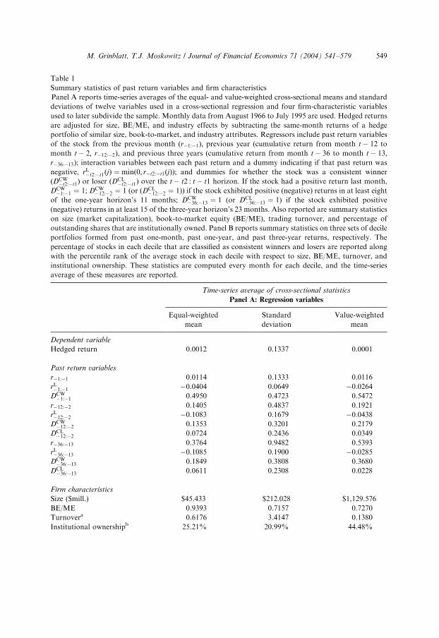
Panel A of Table 1 reports the time series averages of the cross-sectional means(both equal and value weighted) along with the time series averages of the cross-sectional standard deviations for all of the variables used in the regression as well asthe analogously computed means and standard deviations on firm size, BE/ME,turnover, and institutional ownership. (All labels in the tables exclude the t subscriptfor brevity.)

The mean hedged return is close to zero, on the order of 0.1% equal-weighted and0.01% value-weighted. Since this was a relatively good period for stocks, and sincestocks tend to have positive returns, the means of the past return regressors, whichare unhedged, are positive. This also explains why the one- and three-year consistentwinners and losers dummies have averages that are above 10% and below 10%,respectively, with the deviation from 10% larger at the three-year horizon.

The first four columns of Table 1 Panel B report the time series average of theequal- and value-weighted percentile rankings of stocks with various past returnattributes. After classifying stocks each month into deciles for each of the three past-return horizons, the table shows the equal- and value-weighted averages of the rankpercentiles of the stocks’ size, BE/ME ratio, turnover, and institutional ownership.Averages are reported separately for stocks in decile 1 (past losers), the middle eightpast-return deciles, and decile 10 (past winners).

Note that, except for the three-year horizon, stocks in deciles 1 and 10 tend to beof smaller size and BE/ME, and at all horizons, have higher turnover than stocks inthe middle eight deciles. It is not surprising that high turnover is associated withlarge absolute returns. The size and BE/ME comparisons at the three-year horizonare particularly affected by the fact that extreme long-term returns can substantiallyalter a stock’s market capitalization.

Panel B is useful for analyzing the type of firm in the portfolio strategies we willshortly analyze. For example, a typical long-short strategy based on past one-yearreturns would buy stocks in decile 10 and short stocks in decile 1. If value weightingwithin the deciles, the long position would spend an average dollar on a stock with amarket cap percentile of 89.41, a BE/ME percentile of 44.99, a turnover percentile of36.14, and an institutional ownership percentile of 67.30. The short positions in thestrategy would spend an average dollar on a stock with a market cap percentile of70.41, a BE/ME percentile of 40.56, a turnover percentile of 62.97, and an


ARTICLE IN PRESS

Table 1

Summary statistics of past return variables and firm characteristics

Panel A reports time-series averages of the equal- and value-weighted cross-sectional means and standard

deviations of twelve variables used in a cross-sectional regression and four firm-characteristic variables

used to later subdivide the sample. Monthly data from August 1966 to July 1995 are used. Hedged returns

are adjusted for size, BE/ME, and industry effects by subtracting the same-month returns of a hedge

portfolio of similar size, book-to-market, and industry attributes. Regressors include past return variables

of the stock from the previous month ðr�1:�1Þ; previous year (cumulative return from month t � 12 to

month t � 2; r�12:�2), and previous three years (cumulative return from month t � 36 to month t � 13;r�36:�13); interaction variables between each past return and a dummy indicating if that past return was

negative, rL�t2:�t1ðjÞ ¼ minð0; r�t2:�t1ðjÞÞ; and dummies for whether the stock was a consistent winner

ðDCW�t2:�t1Þ or loser ðD

CL�t2:�t1Þ over the t � t2 : t � t1 horizon. If the stock had a positive return last month,

DCW�1:�1 ¼ 1; DCW

�12:�2 ¼ 1 (or ðDCL�12:�2 ¼ 1ÞÞ if the stock exhibited positive (negative) returns in at least eight

of the one-year horizon’s 11 months; DCW�36:�13 ¼ 1 (or DCL

�36:�13 ¼ 1) if the stock exhibited positive

(negative) returns in at least 15 of the three-year horizon’s 23 months. Also reported are summary statistics

on size (market capitalization), book-to-market equity (BE/ME), trading turnover, and percentage of

outstanding shares that are institutionally owned. Panel B reports summary statistics on three sets of decile

portfolios formed from past one-month, past one-year, and past three-year returns, respectively. The

percentage of stocks in each decile that are classified as consistent winners and losers are reported along

with the percentile rank of the average stock in each decile with respect to size, BE/ME, turnover, and

institutional ownership. These statistics are computed every month for each decile, and the time-series

average of these measures are reported.

Time-series average of cross-sectional statistics

Panel A: Regression variables

Equal-weighted Standard Value-weighted

mean deviation mean

Dependent variable

Hedged return 0.0012 0.1337 0.0001

Past return variables

r�1:�1 0.0114 0.1333 0.0116

rL�1:�1 �0.0404 0.0649 �0.0264

DCW�1:�1 0.4950 0.4723 0.5472

r�12:�2 0.1405 0.4837 0.1921

rL�12:�2 �0.1083 0.1679 �0.0438

DCW�12:�2 0.1353 0.3201 0.2179

DCL�12:�2 0.0724 0.2436 0.0349

r�36:�13 0.3764 0.9482 0.5393

rL�36:�13 �0.1085 0.1900 �0.0285

DCW�36:�13 0.1849 0.3808 0.3680

DCL�36:�13 0.0611 0.2308 0.0228

Firm characteristics

Size ($mill.) $45.433 $212.028 $1,129.576

BE/ME 0.9393 0.7157 0.7270

Turnovera 0.6176 3.4147 0.1380

Institutional ownershipb 25.21% 20.99% 44.48%

M. Grinblatt, T.J. Moskowitz / Journal of Financial Economics 71 (2004) 541–579 549

institutional ownership percentile of 59.05. Differences in these percentiles highlightthe importance of subtracting out a benchmark return when studying the linkbetween past and expected returns.

The two rightmost columns in Panel B report the time series average of thepercentage of firms classified as consistent winners and consistent losers. Obviously,the decile 1 firms tend to have more consistent losers and the decile 10 firms tend tohave more consistent winners. At the one-month past return horizon, we are simply

ARTICLE IN PRESS

Time-series average of cross-sectional statistics

Panel B: Decile portfolios

Size BE/ME Turnovera Inst. own.b

rank (%) rank (%) rank (%) rank (%) CW (%) CL (%)

Past one-month returns

Equal-weighted

Low Decile 1 36.98 43.89 69.26 41.58 0.00 100.00

Deciles 2–9 52.82 50.99 45.95 51.68 44.49 55.51

High Decile 10 40.77 48.23 63.05 45.17 99.56 0.44

Value-weighted

Decile 1 80.96 42.21 47.09 64.92 0.00 100.00

Deciles 2–9 93.78 48.24 23.68 70.54 54.42 45.58

Decile 10 83.96 46.50 40.31 66.01 99.52 0.48

Past one-year returns

Equal-weighted

Decile 1 29.26 41.82 76.37 40.28 0.01 33.62

Deciles 2–9 52.55 51.18 45.49 51.49 8.83 4.67

Decile 10 50.48 48.86 59.54 48.05 34.16 0.08

Value-weighted

Decile 1 70.41 40.56 62.97 59.05 0.00 41.38

Deciles 2–9 93.68 48.36 23.64 70.84 18.89 3.39

Decile 10 89.41 44.99 36.14 67.30 59.24 0.01

Past three-year returns

Equal-weighted

Decile 1 26.69 55.21 77.69 41.32 0.04 30.43

Deciles 2–9 51.67 50.96 46.44 50.39 11.18 3.53

Decile 10 59.94 37.42 50.78 55.67 44.31 0.11

Value-weighted

Decile 1 69.22 57.38 62.79 58.68 0.15 36.85

Deciles 2–9 93.52 49.79 23.65 70.08 31.17 2.26

Decile 10 92.00 34.83 31.23 72.65 76.63 0.01

aTurnover is defined separately for NYSE-AMEX and NASDAQ stocks due to different conventions in

recorded volume on the exchanges. The turnover numbers are scaled by the means for each exchange in

order to account for this institutional discrepancy. Calculated from January 1976 onward for NYSE-

AMEX firms and January 1983 onward for NASDAQ firms.bCalculated from January 1981 onward, when data became available.

Table 1. (Continued )


classifying whether the prior month’s return was positive or negative. Hence, thepercentages for consistent winners and losers sum to one.

3. Results from Fama-MacBeth cross-sectional regressions

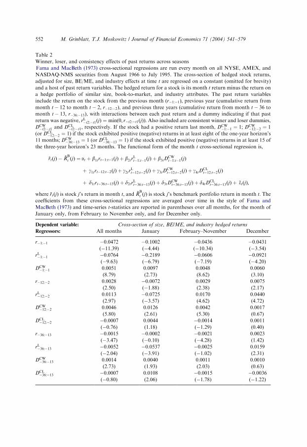
Table 2 reports the time series average from August 1966 to July 1995 of themonthly coefficients from the cross-sectional regression in Eq. (1) along with Famaand MacBeth (1973) time-series t-statistics. While the Compustat data begins inAugust 1963, we need three years of past return data to compute one of ourvariables. No CRSP-listed stock has this prior to August 1966 and no CRSP-listedNASDAQ firm has this prior to January 1976. We end the estimation in July 1995,reflecting the most recent data in the first draft of this paper. At the suggestion of ananonymous referee, we reserved the August 1995 to December 1999 period for out-of-sample tests.

The column labels identify whether the coefficients are averaged over all months,Januaries only, February–November only, or December only. The rows in Table 2correspond to regressors. The three return rows, labeled r�1:�1; r�12:�2; and r�36:�13;show a strong one-month reversal effect, a weaker one-year momentum effect, and astill weaker three-year reversal effect, respectively, both when averaging thecoefficients over all months and when averaging only from February to November.All of these effects are statistically significant. The three loser return coefficients areall of the same sign as the return coefficients, and statistically significant. Thissuggests that the effects of return persistence and reversals are exacerbated fornegative past returns. Again, this is the case for all months as well as February–November.

Hong et al. (2000) and Lee and Swaminathan (2000) show that portfolios of losingstocks subsequently underperform a portfolio of average performing stocks to agreater degree than winning stocks outperform average stocks. However, when thecharacteristics of average stocks differ dramatically from those of past winning andlosing stocks (as shown in Table 1), the returns of stocks with the past returns in themiddle grouping are not an appropriate benchmark for either past winning or pastlosing stocks. Our regression specification and use of hedged returns of stocks withexpected values of zero under the null, provide cleaner ways to assess whether theshort or the long side drives the abnormally large profit of technical tradingstrategies. The hedged returns of the stocks predicted to have the highest (lowest)returns indicate whether the long (short) side of an investment strategy based on pastreturns is profitable and their magnitude quantifies the degree of profitability.

3.1. Winner consistency

One of the more striking findings is that all 12 consistent winners coefficients inTable 2 are positive and most are statistically significant. This indicates that for allthree horizons and all three seasonal subperiods, as well as the overall sample,consistent winners outperform other stocks, ceteris paribus. At the one-year horizon,


ARTICLE IN PRESS

Table 2

Winner, loser, and consistency effects of past returns across seasons

Fama and MacBeth (1973) cross-sectional regressions are run every month on all NYSE, AMEX, and

NASDAQ-NMS securities from August 1966 to July 1995. The cross-section of hedged stock returns,

adjusted for size, BE/ME, and industry effects at time t are regressed on a constant (omitted for brevity)

and a host of past return variables. The hedged return for a stock is its month t return minus the return on

a hedge portfolio of similar size, book-to-market, and industry attributes. The past return variables

include the return on the stock from the previous month ðr�1:�1Þ; previous year (cumulative return from

month t � 12 to month t � 2; r�12:�2), and previous three years (cumulative return from month t � 36 to

month t � 13; r�36:�13), with interactions between each past return and a dummy indicating if that past

return was negative, rL�t2:�t1ðjÞ ¼ minð0; r�t2:�t1ðjÞÞ: Also included are consistent winner and loser dummies,

DCW�t2:�t1 and DCL

�t2:�t1; respectively. If the stock had a positive return last month, DCW�1:�1 ¼ 1; DCW

�12:�2 ¼ 1

(or DCL�12:�2 ¼ 1) if the stock exhibited positive (negative) returns in at least eight of the one-year horizon’s

11 months; DCW�36:�13 ¼ 1 (or DCL

�36:�13 ¼ 1) if the stock exhibited positive (negative) returns in at least 15 of

the three-year horizon’s 23 months. The functional form of the month t cross-sectional regression is,

*rtðjÞ � *RB

t ðjÞ ¼ at þ b1trt�1:t�1ðjÞ þ b2trLt�1:t�1ðjÞ þ b3tD

CWt�1:t�1ðjÞ

þ g1trt�12:t�2ðjÞ þ g2trLt�12:t�2ðjÞ þ g3tD

CWt�12:t�2ðjÞ þ g4tD

CLt�12:t�2ðjÞ

þ d1trt�36:t�13ðjÞ þ d2trLt�36:t�13ðjÞ þ d3tD

CWt�36:t�13ðjÞ þ d4tD

CLt�36:t�13ðjÞ þ *etðjÞ;

where *rtðjÞ is stock j’s return in month t; and *RB

t ðjÞ is stock j’s benchmark portfolio return in month t: Thecoefficients from these cross-sectional regressions are averaged over time in the style of Fama and

MacBeth (1973) and time-series t-statistics are reported in parentheses over all months, for the month of

January only, from February to November only, and for December only.

Dependent variable: Cross-section of size, BE/ME, and industry hedged returns

Regressors: All months January February–November December

r�1:�1 �0.0472 �0.1002 �0.0436 �0.0431

(�11.39) (�4.44) (�10.34) (�3.54)

rL�1:�1 �0.0764 �0.2189 �0.0606 �0.0921

(�9.63) (�6.79) (�7.19) (�4.20)

DCW�1:�1 0.0051 0.0097 0.0048 0.0060

(8.79) (2.73) (8.62) (3.10)

r�12:�2 0.0028 �0.0072 0.0029 0.0075

(2.50) (�1.88) (2.38) (2.17)

rL�12:�2 0.0113 �0.0725 0.0170 0.0440

(2.97) (�3.57) (4.62) (4.72)

DCW�12:�2 0.0046 0.0126 0.0042 0.0017

(5.80) (2.61) (5.30) (0.67)

DCL�12:�2 �0.0007 0.0044 �0.0014 0.0011

(�0.76) (1.18) (�1.29) (0.40)

r�36:�13 �0.0015 �0.0002 �0.0021 0.0023

(�3.47) (�0.10) (�4.28) (1.42)

rL�36:�13 �0.0052 �0.0537 �0.0025 0.0159

(�2.04) (�3.91) (�1.02) (2.31)

DCW�36:�13 0.0014 0.0040 0.0011 0.0010

(2.73) (1.93) (2.03) (0.63)

DCL�36:�13 �0.0007 0.0108 �0.0015 �0.0036

(�0.80) (2.06) (�1.78) (�1.22)


the marginal impact of being a consistent winner is 46 basis points per month.Consistent losers have little impact on returns, suggesting that the impact of winnerconsistency is not due to the lower volatility associated with consistency as astatistical proxy for a lower (constant) variance stock. Rather, it reflects a morecomplex past returns effect.

We can speculate about the potential source of the consistency effect. Forexample, Grinblatt and Han (2002) argue that ‘‘y‘consistent’ winning (or‘consistent losing’) stocks necessarily have investors who acquired the stock at abasis below the current price—thus experiencing a capital gain (or, in the case ofconsistent losers, a capital loss).’’ In their model, such aggregate gains (or losses)cannot be undone by arbitrageurs and lead to reference price updates that revert tofundamentals. This generates mean reversion in the spread between the equilibriumprice of a stock and its fundamental value, and, as a consequence, momentum. InWatkins (2002), firms have identical future cash flows but unknown discount rates.Investors have asymmetric information about these discount rates. In a sequentiallearning model, firms that have experienced consistent price increases tend to bethose experiencing dissemination of their low discount rate type and vice versa. Boththe Grinblatt and Han (2002) and Watkins (2002) models point to a consistentwinners and a consistent losers effect. The absence of a consistent losers effect in oursample, rather than being a rejection of these models, may simply highlight theimportant price effects of tax-loss trading, which probably apply more to consistentlosers. Overlaying tax-loss trading effects on both of these models could generate aconsistency effect only in winning stocks. It is worth noting here that Watkins(2002), using CRSP monthly data from 1927 on, shows both a winner and a loserconsistency effect. It is difficult to assess whether his findings, which are based onraw returns, would stand up to the controls we use.

3.2. Seasonal patterns and tax-loss selling

The seasonal pattern in Table 2 is also particularly interesting, with both Januaryreturn coefficients being negative for the one-year variables. Jegadeesh and Titman(1993) identify positive profits for momentum strategies in every month exceptJanuary, for which they show significant negative profits, and find strongermomentum profits in April, November, and December. They suggest that thenegative January profits from a momentum strategy are due to the tendency ofwinners to trade at the ask price and losers to sell at the bid at the close of the lasttrading day in December (see Keim, 1989). This will induce negative autocorrelationin monthly returns from December to January. Since we skip a month beforecomputing our past one-year stock returns (as well as control for one-month returneffects in the regression), the seasonal patterns observed here are not susceptible tothis bid–ask bounce, yet exhibit the same pattern. Moreover, Jegadeesh and Titman(1993) do not separate out the seasonal effects of winners and losers. As Table 2shows, the asymmetries between winner and loser return effects are quite importantand help to assess the degree to which other explanations, such as tax-loss trading,


account for the relation between past returns and expected returns, as we will seeshortly.

Can the seasonal pattern in the coefficients reported in Table 2 be explained bytax-loss selling (an end-of-December sell-off of losing stocks for tax purposes) whichis magnified by the lower liquidity in financial markets at the end of the year?Although evidence of high returns in January supports this story, to date there hasbeen relatively little evidence of a December effect for stock returns. However, Table2 shows a significant December persistence effect for both one- and three-year losingstocks. If the market for such stocks is particularly illiquid at the end of December,then tax-loss trading behavior could generate price patterns that are consistent withloser persistence in December and reversals in January. The observed seasonalpattern in losing stocks, both over the one- and three-year past return horizons, asrepresented by the sums of the coefficients on the pair r�12:�2 and rL�12:�2 and on thepair r�36:�13; rL�36:�13; exhibit this pattern.

The effect of tax-loss trading on the seasonal return pattern of winning stocks ismore ambiguous. On the one hand, full utilization of the tax write-offs for realizedcapital losses requires that there be a realized capital gain of equal or greater size. Onthe other hand, investors have generally been able to carry losses backward andforward to other tax years to some extent. These investors, as well as those with nocapital losses, should be reluctant to sell winning stocks to avoid realizing capitalgains. The coefficient on the past winning returns over both the one- and three-yearhorizons, given in the rows for r�12:�2 and r�36:�13; are largest in December (with apositive coefficient rather than the normally negative coefficient, as noted above, forthe three-year past return horizon). This coefficient pattern argues for deferral oflarge tax-related December net sales in the aggregate when only a few investorsexperience a large capital gain in the stock. On the other hand, being a consistentwinner in December is more indicative of a large number of investors looking at thestock as a winner at the turn of the year. To the extent that a significant fraction ofthese investors need the gain realization to take advantage of a loss, we would expecta lower coefficient on the consistent winners dummy in December.

The interpretation of the consistent winners coefficient in December hinges on theexistence of a degree of relative illiquidity in stock markets at the turn of the year, sothat tax-related selling can affect prices. Evidence from Table 2 supports theconjecture that the turn of the year coincides with a particularly illiquid market,especially for past losers. The coefficients on both r�1:�1 and rL�1:�1; possibly due to aliquidity effect, are most negative in January and slightly more negative than usual inDecember.

The prevailing wisdom, since DeBondt and Thaler (1985) and Chopra et al.(1992), is that the three-year reversal is primarily driven by extreme losers. This iscertainly the case for January, as DeBondt and Thaler (1985) and Chopra et al.(1992) also note. The January coefficient on r�36:�13 is insignificant, indicating theabsence of a three-year winner effect on January returns. However, this hypothesisdoes not apply to the rest of the year. From February through November there is nodifference in the impact of past three-year positive and past three-year negativereturns, as evidenced by the insignificant coefficient on rL�36:�13: In addition, the sum


of the December three-year return coefficient and the loser return coefficient is notonly positive, indicating persistence rather than reversals, but it is about eight timesthe size of the return coefficient (the impact of the positive returns) in December. Asdiscussed later, the positive three-year losers coefficient in December is indicative ofyear-end tax-loss selling.

DeBondt and Thaler (1985, 1987) and Chopra et al. (1992) claim long-termreversals are not solely contained in January and are not due to tax-motivatedtrading. Rather, they argue that investor overreaction is the likely explanation.Conversely, Chan (1988), Ball and Kothari (1989), and Fama and French (1996)argue that rational time-variation in expected returns can explain these reversals. Byseparating long-term reversals from other past return effects and using hedgedreturns to account for confounding return premia, we provide a more powerful testof the tax-loss selling hypothesis.

3.3. The relation between past return horizons

Recent literature posits a link between the effects of various past return horizons. Forinstance, Daniel et al. (1998), Barberis et al. (1998), and Hong and Stein (1999) allprovide models that tie intermediate-term momentum to long-term reversals undervarious theories of irrational investor behavior. Hong et al. (2000), Lee andSwaminathan (2000), and Jegadeesh and Titman (2001) claim that such a link existsin the data. However, Jegadeesh and Titman (2001), despite showing that the profitsearned from momentum stocks dissipate by the end of a five-year holding period, arequite cautious in their interpretation, noting that horizon length, time period studied,and benchmarking of returns plays an important role in the inference about the linkage.

By analyzing nonoverlapping return horizons simultaneously, and carefullycontrolling for confounding return premia, our study provides a cleaner test of thepotential link between momentum and reversals. If the one-year past returns effectdetermines the three-year past returns effect, then intermediate-term momentum isprobably an overreaction to past news. This would considerably limit the set of validtheories that could explain these phenomena. First, the fact that each past returnhorizon variable shows up significantly in our cross-sectional regressions suggeststhat at least part of these effects are independent from one another. Second, inunreported results, we ran separate regressions for each past return horizon andfound the coefficients to be almost identical to those from the full regression ofTable 2. This suggests significant independence among the various horizons. Finally,the fact that the long-term reversals are almost exclusively driven by long-term losersin January, yet momentum is prevalent throughout the calendar year, also suggeststhat at least part of these past return horizon effects are unrelated.

3.4. Comparing winner consistency effects with momentum and reversals

Table 2 indicates that being a consistent winner enhances average returns. Toassess the economic relevance of being a consistent winner, and to facilitatecomparisons with the pure momentum and reversal effect, Table 3 reports average


ARTIC

LEIN

PRES

S

Table 3

The economic importance of winner consistency

Stocks are ranked each month by past returns and grouped into rank-based decile portfolios, with decile 10 having the highest past return. Both equal- and

value-weighted decile portfolio returns of the hedged (with respect to size, BE/ME, and industry) positions in stocks are computed over the August 1966 to

July 1995 time period. The first five columns report value-weighted results and the next five equal-weighted results. The first column reports the time-series

average return of all stocks across all past returns and the next four columns report the time-series average of each of the first and last two return deciles.

Average profits are reported for all months, for the month of January only, February–November, and December only. Panel A ranks stocks based on their

past one-year return from month t � 2 to t � 12; Panel B ranks stocks based on their past three-year return from month t � 13 to t � 36: Each portfolio is

then broken down into those stocks that were not consistent winners (defined as fewer than eight out of 11 positive past return months in Panel A and fewer

than 15 out of 23 positive past return months in Panel B), and the return on the portfolio of these stocks only (where the portfolio is re-weighted to sum to

one) is reported. In a similar manner profits are reported for the past return deciles containing only consistent winners defined in Panel A (Panel B) as eight

(15) or more and nine (18) or more positive return months out of the past 11 (23).

Past return decile portfolios

Value-weighted Equal-weighted

All 1 2 9 10 All 1 2 9 10

Panel A: Past one-year effect and winner consistency

All 0.0003 �0.0018 �0.0010 0.0031 0.0054 0.0010 �0.0018 �0.0011 0.0044 0.0060

Jan. 0.0014 0.0070 0.0069 �0.0001 �0.0059 0.0006 0.0004 �0.0009 �0.0128 �0.0133

Feb.–Nov. �0.0001 �0.0026 �0.0017 0.0032 0.0059 0.0012 �0.0015 �0.0008 0.0057 0.0069

Dec. 0.0025 �0.0017 �0.0012 0.0047 0.0081 0.0002 �0.0058 �0.0037 0.0084 0.0154

Non-consistent winner stocks only

All 0.0001 �0.0019 �0.0011 0.0029 0.0041 0.0005 �0.0018 �0.0011 0.0041 0.0045

Jan. 0.0019 0.0070 0.0068 0.0013 �0.0034 0.0021 0.0005 �0.0009 �0.0112 �0.0111

Feb.–Nov. �0.0003 �0.0026 �0.0018 0.0028 0.0044 0.0005 �0.0015 �0.0008 0.0052 0.0049

Dec. 0.0024 �0.0033 �0.0018 0.0050 0.0069 �0.0010 �0.0058 �0.0036 0.0083 0.0146

Consistent winner stocks with at least 8 out of 11 past positive returns only

All 0.0016 0.0059 0.0022 0.0042 0.0058 0.0059 0.0017 0.0012 0.0063 0.0091

Jan. �0.0027 0.0013 �0.0007 �0.0076 �0.0072 �0.0125 �0.0058 �0.0027 �0.0144 �0.0117

Feb.–Nov. 0.0018 0.0039 0.0010 0.0051 0.0063 0.0073 0.0026 0.0012 0.0082 0.0102

Dec. 0.0032 0.0288 0.0146 0.0083 0.0090 0.0114 -0.0009 0.0016 0.0089 0.0176

M.

Grin

bla

tt,T

.J.

Mo

sko

witz

/J

ou

rna

lo

fF

ina

ncia

lE

con

om

ics7

1(

20

04

)5

41

–5

79

556

ARTIC

LEIN

PRES

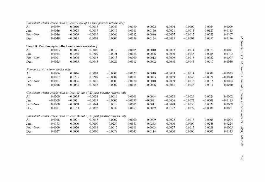
SConsistent winner stocks with at least 9 out of 11 past positive returns only

All 0.0039 �0.0010 �0.0013 0.0049 0.0080 0.0072 �0.0004 �0.0009 0.0064 0.0099

Jan. �0.0046 �0.0028 0.0017 �0.0016 �0.0061 �0.0156 �0.0021 �0.0013 �0.0127 �0.0143

Feb.–Nov. 0.0046 �0.0009 �0.0016 0.0060 0.0082 0.0086 �0.0007 �0.0012 0.0083 0.0107

Dec. 0.0049 �0.0015 0.0001 0.0004 0.0079 0.0124 �0.0015 �0.0004 0.0057 0.0196

Panel B: Past three-year effect and winner consistency

All 0.0003 0.0015 0.0000 0.0012 �0.0005 0.0010 �0.0003 �0.0014 0.0013 �0.0011

Jan. 0.0014 0.0286 0.0209 �0.0021 �0.0084 0.0006 0.0090 0.0045 �0.0085 �0.0102

Feb.–Nov. �0.0001 �0.0006 �0.0016 0.0013 0.0000 0.0012 �0.0009 �0.0018 0.0022 �0.0007

Dec. 0.0025 �0.0033 �0.0043 0.0029 0.0013 0.0002 �0.0040 �0.0043 0.0017 0.0030

Non-consistent winner stocks only

All 0.0006 0.0016 0.0001 �0.0003 �0.0023 0.0010 �0.0003 �0.0014 0.0008 �0.0025

Jan. 0.0057 0.0285 0.0209 �0.0002 0.0011 0.0023 0.0089 0.0045 �0.0071 �0.0080

Feb.–Nov. �0.0001 �0.0006 �0.0016 �0.0003 �0.0030 0.0010 �0.0009 �0.0018 0.0015 �0.0024

Dec. 0.0018 �0.0035 �0.0043 0.0002 �0.0018 �0.0006 �0.0041 �0.0043 0.0011 0.0010


All 0.0000 �0.0055 �0.0034 0.0019 0.0001 0.0004 �0.0038 �0.0029 0.0024 0.0002

Jan. �0.0069 �0.0021 �0.0017 �0.0006 �0.0098 �0.0091 �0.0036 �0.0073 �0.0001 �0.0115

Feb.–Nov. 0.0000 �0.0068 �0.0044 0.0019 0.0005 0.0011 �0.0049 �0.0030 0.0029 0.0009

Dec. 0.0071 0.0153 0.0093 0.0032 0.0063 0.0039 0.0192 0.0079 �0.0008 0.0061


All �0.0018 0.0021 0.0013 �0.0007 0.0000 �0.0009 0.0022 0.0013 0.0005 �0.0004

Jan. �0.0173 0.0000 0.0000 �0.0230 �0.0143 �0.0233 0.0000 0.0000 �0.0248 �0.0224

Feb.–Nov. �0.0009 0.0026 0.0016 0.0017 0.0011 0.0003 0.0027 0.0017 0.0028 0.0005

Dec. 0.0027 0.0000 0.0000 �0.0078 0.0043 0.0114 0.0000 0.0000 0.0002 0.0145

M.

Grin

bla

tt,T

.J.

Mo

sko

witz

/J

ou

rna

lo

fF

ina

ncia

lE

con

om

ics7

1(

20

04

)5

41

–5

79

557

monthly returns of investment portfolios constructed on the basis of past returns andwinner consistency. First, we sort firms into decile portfolios based on their pastreturns and then on the number of winning months. Columns correspond to the pastreturn decile portfolios, with decile 10 having the highest past return. Rowscorrespond to three classifications of the number of positive past return months andthree seasons (January, February–November, and December). The left-hand side ofthe table reports value-weighted results and the right-hand side equal-weightedresults. Panel A reports results for the one-year past return horizon and Panel Breports results for the three-year past return horizon.

Since consistency will only affect the extremes, we report results only for deciles 1,2, 9, and 10. Attempting inferences from past return portfolios 3–8 is a futile exercise,since few consistent winning firms exist in these portfolios. Similarly, any sensibleanalysis of this table should focus on numbers that correspond to well-diversifiedportfolios. For instance, the number of consistent winners in deciles 1 and 2 isnegligible. Also, reporting on levels of consistency that are nearly impossible toachieve makes little sense. In Panel A, for example, hardly any firms experience atleast ten (of a possible 11) positive past return months, even in past return deciles 9and 10. The same caveat applies to certain levels of consistency in Panel B, as simplecombinatorics would suggest.

Table 3 Panel A, which compares consistency and intermediate-horizonmomentum, suggests that consistency is as important as the past return per se.The first row of this panel presents the pure momentum effect. Here, equal-weightedportfolios 9 and 10 earn hedged returns of 44 and 60 basis points per month,respectively (31 basis points and 54 basis points per month, respectively, when valueweighting). Different rows in this panel break these numbers down by the number ofwinning months. Focusing first on decile 10 firms, we note that (on an equal-weighted basis) 67% of the 60 basis-point hedged return comes from firms that arenot consistent winners, while 33% comes from consistent winning firms, defined tobe firms with at least eight positive monthly returns within months t � 2 to t � 12:Also, 13% of the return is derived from extremely consistent winning firms, thosewith at least nine positive monthly returns within these months. The firms inequal-weighted portfolio 10 that are not consistent winners earned 45 basispoints per month, the consistently winning firms earned 91 basis points per month,and the extremely consistent winning firms in decile 10 earned 99 basis points permonth.

The regression coefficient on DCW�12:�2 in Table 2 indicates that being a consistent

winner over the past year adds 46 basis points per month to a return. Table 3 PanelA suggests that being a consistent winner enhances the performance of stocks withinequal-weighted decile 10 by 46 basis points per month, with the spread increasing to54 basis points per month when we focus on approximately the 13% most consistentstocks, approximately doubling the past return effect.

The numbers are approximately the same if we focus only on February–November, whether equal weighting or value weighting. Because the excellentDecember performance of these high return firms (overall, as well as in the threesubcategories of firms) slightly outweighs their poor performance in January, each of


the decile 10 numbers goes up by four to nine basis points if January and Decemberare excluded.

The spreads between the hedged returns of consistent winning firms and firms thatare not consistent winners are less dramatic in the decile 9 past return portfolio. Theyare 30 basis points per month when we exclude January and December and 22 basispoints per month over all months.

In comparison with the equal-weighted numbers above, value weighting reducesthe additional return enhancement to momentum generated by being a consistentwinner, but only moderately from February–November. The seasonal differencearises because the large-cap firms in deciles 9 and 10 that are not consistent winnersexhibit either surprisingly modest or no January reversals relative to theirbenchmark. We are reluctant to draw conclusions from this, particularly for anyaverage return associated with a single month.

On an equal-weighted basis, the February–November hedged returns of stockswith at least eight of the 11 relevant months being positive is 73 basis points permonth, while with nine or more months being positive, the hedged return modestlyjumps to 86 basis points per month. These numbers are clearly of the same order ofmagnitude as the past returns effect per se.

Table 3 Panel B tells a similar story for the long-term reversal effect. Outside ofJanuary, there is little reversal in equal-weighted portfolio 10, unless one separatesout the consistent winners. A modest reversal from February to November doesexist, but only for the 59% of stocks that are not consistent winners. The latterstocks earn a February–November hedged return of �24 basis points per month(�30 basis points per month when value weighted). This is 33 basis points per monthless than the stocks in the same portfolio with at least 15 positive returns in therelevant 23 months (59% of portfolio 10) and 29 basis points per month less than the7% of stocks in the same portfolio with at least 18 positive returns in the relevant 23months. In decile 9, the spread between consistent winning stocks and stocks that arenot consistent winners is about one-half this size.

4. Economic significance of the past expected-return relation

To further examine the economic importance of the relation between the past patternof returns and expected returns, we form trading strategies based on the insights fromthe previous regressions. We use the predicted returns from the Fama-MacBethregressions of Table 2 to rank stocks and form decile portfolios with decile 10 containingstocks with the highest predicted returns. Rankings are determined by the beginning-of-month regressor values for the corresponding stocks, and we use average coefficientsfrom the appropriate sample of months (as discussed below) to weight the regressorvalues. Decile portfolios either equal or value weight the stocks within each decile rank.

4.1. Profitability and risk of trading strategies from stock rankings

Panel A of Table 4 reports average monthly hedged returns along with annualizedstandard deviations for each corresponding decile portfolio (both equal and value


ARTIC

LEIN

PRES

S

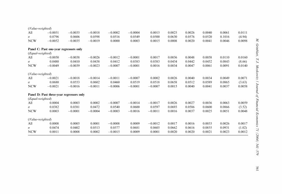
Table 4

Economic significance of the relation between past and expected returns

Average monthly returns and annualized standard deviations ðsÞ of 10 zero-cost portfolios are reported over the August 1966 to July 1995 time period. Using

the predicted returns from the multivariate regression of Table 2, stocks are ranked each month and grouped into rank-based decile portfolios, with decile 10

having the highest predicted return. Both equal- and value-weighted decile portfolio returns of the hedged (with respect to size, BE/ME, and industry)

positions in stocks are computed. The time-series average of the regression coefficients are used to score stocks, where January coefficients are used for

January rankings, February–November coefficients for February–November rankings, and December coefficients for December rankings. Time-series

average returns and annualized standard deviations are reported over all months for each decile, along with the difference between decile 10 (highest predicted

return) and decile 1 (lowest predicted return) and the corresponding t-statistic for this difference. Panel A uses all regression coefficients to score and rank

stocks. Panel B excludes the three regression coefficients corresponding to the one-month past return regressors to rank stocks. Panel C uses only the four

regression coefficients corresponding to one-year past return regressors to rank stocks, and Panel D uses only the four regression coefficients corresponding to

three-year past return regressors to rank stocks. Also reported in each panel are the equal- and value-weighted profits from ranking systems that ignore (zero

out) the coefficients on the consistent winners dummy variables denoted as NCW.

Decile portfolios 10�1

(t-stat.)

1 2 3 4 5 6 7 8 9 10

Panel A: All regressors

(Equal-weighted)

All �0.0065 �0.0046 �0.0026 �0.0007 0.0009 0.0016 0.0027 0.0041 0.0076 0.0215 0.0280

s 0.0518 0.0428 0.0430 0.0404 0.0375 0.0328 0.0336 0.0325 0.0462 0.1052 (12.85)

NCW �0.0066 �0.0045 �0.0029 �0.0011 0.0011 0.0017 0.0029 0.0036 0.0069 0.0196 0.0262

(Value-weighted)

All �0.0047 �0.0035 �0.0023 �0.0012 0.0012 0.0012 0.0029 0.0051 0.0062 0.0092 0.0139

s 0.0693 0.0456 0.0465 0.0520 0.0486 0.0464 0.0490 0.0532 0.0693 0.1104 (6.48)

NCW �0.0048 �0.0038 �0.0022 �0.0010 0.0007 0.0010 0.0025 0.0049 0.0050 0.0078 0.0126

Panel B: Exclude past one-month regressors

(Equal-weighted)

All �0.0055 �0.0039 �0.0023 �0.0002 0.0011 0.0019 0.0027 0.0043 0.0056 0.0113 0.0168

s 0.0587 0.0444 0.0444 0.0385 0.0347 0.0354 0.0344 0.0414 0.0437 0.0984 (7.77)

NCW �0.0053 �0.0041 �0.0031 �0.0002 0.0008 0.0020 0.0026 0.0034 0.0055 0.0094 0.0147

M.

Grin

bla

tt,T

.J.

Mo

sko

witz

/J

ou

rna

lo

fF

ina

ncia

lE

con

om

ics7

1(

20

04

)5

41

–5

79

560

ARTIC

LEIN

PRES

S

(Value-weighted)

All �0.0051 �0.0035 �0.0018 �0.0002 �0.0004 0.0015 0.0025 0.0026 0.0040 0.0061 0.0111

s 0.0796 0.0606 0.0598 0.0516 0.0549 0.0500 0.0630 0.0576 0.0520 0.1016 (4.94)

NCW �0.0052 �0.0035 �0.0019 0.0000 0.0003 0.0015 0.0008 0.0020 0.0041 0.0046 0.0098

Panel C: Past one-year regressors only

(Equal-weighted)

All �0.0050 �0.0038 �0.0026 �0.0012 �0.0001 0.0017 0.0036 0.0048 0.0058 0.0110 0.0160

s 0.0480 0.0410 0.0438 0.0412 0.0383 0.0383 0.0434 0.0442 0.0452 0.0843 (8.66)

NCW �0.0049 �0.0039 �0.0023 �0.0007 �0.0001 0.0016 0.0034 0.0047 0.0061 0.0091 0.0140

(Value-weighted)

All �0.0021 �0.0018 �0.0014 �0.0011 �0.0007 0.0002 0.0026 0.0040 0.0034 0.0049 0.0071

s 0.0680 0.0553 0.0602 0.0460 0.0519 0.0518 0.0658 0.0512 0.0589 0.0865 (3.63)

NCW �0.0021 �0.0016 �0.0011 �0.0006 �0.0001 �0.0007 0.0015 0.0040 0.0041 0.0037 0.0058

Panel D: Past three-year regressors only

(Equal-weighted)

All 0.0004 0.0003 0.0002 �0.0007 �0.0014 �0.0017 0.0026 0.0027 0.0036 0.0063 0.0059

s 0.0382 0.0381 0.0472 0.0540 0.0600 0.0597 0.0693 0.0586 0.0600 0.0866 (3.52)

NCW 0.0003 �0.0001 �0.0004 �0.0003 �0.0016 �0.0011 0.0016 0.0037 0.0025 0.0051 0.0048

(Value-weighted)

All 0.0008 0.0005 0.0001 �0.0008 0.0009 �0.0012 0.0017 0.0016 0.0033 0.0026 0.0017

s 0.0474 0.0402 0.0513 0.0577 0.0681 0.0605 0.0662 0.0616 0.0855 0.0931 (1.02)

NCW 0.0011 0.0008 0.0002 �0.0015 0.0009 0.0001 0.0020 0.0020 0.0021 0.0023 0.0012

M.

Grin

bla

tt,T

.J.

Mo

sko

witz

/J

ou

rna

lo

fF

ina

ncia

lE

con

om

ics7

1(

20

04

)5

41

–5

79

561

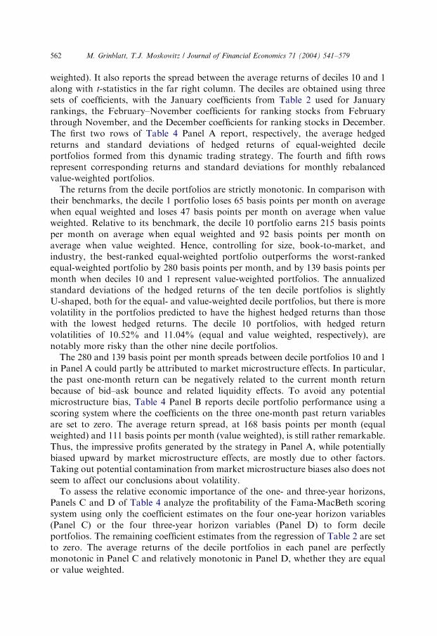
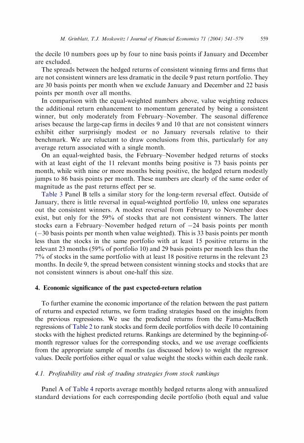
weighted). It also reports the spread between the average returns of deciles 10 and 1along with t-statistics in the far right column. The deciles are obtained using threesets of coefficients, with the January coefficients from Table 2 used for Januaryrankings, the February–November coefficients for ranking stocks from Februarythrough November, and the December coefficients for ranking stocks in December.The first two rows of Table 4 Panel A report, respectively, the average hedgedreturns and standard deviations of hedged returns of equal-weighted decileportfolios formed from this dynamic trading strategy. The fourth and fifth rowsrepresent corresponding returns and standard deviations for monthly rebalancedvalue-weighted portfolios.

The returns from the decile portfolios are strictly monotonic. In comparison withtheir benchmarks, the decile 1 portfolio loses 65 basis points per month on averagewhen equal weighted and loses 47 basis points per month on average when valueweighted. Relative to its benchmark, the decile 10 portfolio earns 215 basis pointsper month on average when equal weighted and 92 basis points per month onaverage when value weighted. Hence, controlling for size, book-to-market, andindustry, the best-ranked equal-weighted portfolio outperforms the worst-rankedequal-weighted portfolio by 280 basis points per month, and by 139 basis points permonth when deciles 10 and 1 represent value-weighted portfolios. The annualizedstandard deviations of the hedged returns of the ten decile portfolios is slightlyU-shaped, both for the equal- and value-weighted decile portfolios, but there is morevolatility in the portfolios predicted to have the highest hedged returns than thosewith the lowest hedged returns. The decile 10 portfolios, with hedged returnvolatilities of 10.52% and 11.04% (equal and value weighted, respectively), arenotably more risky than the other nine decile portfolios.

The 280 and 139 basis point per month spreads between decile portfolios 10 and 1in Panel A could partly be attributed to market microstructure effects. In particular,the past one-month return can be negatively related to the current month returnbecause of bid–ask bounce and related liquidity effects. To avoid any potentialmicrostructure bias, Table 4 Panel B reports decile portfolio performance using ascoring system where the coefficients on the three one-month past return variablesare set to zero. The average return spread, at 168 basis points per month (equalweighted) and 111 basis points per month (value weighted), is still rather remarkable.Thus, the impressive profits generated by the strategy in Panel A, while potentiallybiased upward by market microstructure effects, are mostly due to other factors.Taking out potential contamination from market microstructure biases also does notseem to affect our conclusions about volatility.

To assess the relative economic importance of the one- and three-year horizons,Panels C and D of Table 4 analyze the profitability of the Fama-MacBeth scoringsystem using only the coefficient estimates on the four one-year horizon variables(Panel C) or the four three-year horizon variables (Panel D) to form decileportfolios. The remaining coefficient estimates from the regression of Table 2 are setto zero. The average returns of the decile portfolios in each panel are perfectlymonotonic in Panel C and relatively monotonic in Panel D, whether they are equalor value weighted.


A comparison of Panels C and D indicates that the past one-year horizon, whichgenerates a momentum strategy in all but January, has the stronger effect with aspread of 71 basis points per month between value-weighted deciles 10 and 1. The 17basis point spread for the pure three-year horizon strategy, when value-weighting, isonly about one-fourth the size of the one-year strategy’s profitability. This could bebecause the three-year reversal effect is concentrated in the extremes and largelyapplies to small-cap stocks. Equal weighting within the deciles generates a 59 basispoint spread between deciles 10 and 1 in Panel D. However, momentum is also astronger economic effect among small stocks. Equally weighting the stocks withinthe deciles of Panel C also generates a 160 basis point spread between deciles 10 and1. This suggests that despite the spread moderation induced by value weighting, thepast one year has a stronger effect on expected stock returns than the past threeyears.

4.2. The importance of winner consistency

The last section showed that being a consistent winner seems to enhanceprofitability. This is the case for the momentum and reversal strategies generated bythe more complex ranking system here as it was for the simple momentum andreversal strategies studied in Table 3. To demonstrate this, Table 4 reports value- andequal-weighted decile portfolios that exclude consistent winners’ criteria (denoted asNCW rows). This corresponds to sorting into decile portfolios using a scoring systemwith coefficients identical to those in the rest of the corresponding panel, except thatthe coefficients on all consistent winners’ dummy variables are set to zero. In general,the spread between the decile 10 and decile 1 portfolios decline, typically on the orderof 10–20 basis points per month. They are similar whether value or equal weightingwithin the decile portfolios.

The relatively small decline in spreads is not a reflection of the marginal impact ofwinner consistency, however. A 40–50 basis-point per-month winner-consistencyeffect can easily generate a 10–20 basis point spread decline in the NCW row. Thisdecline measures a netting of a return effect against a winner consistency effect. Also,the spread decline is diluted in that deciles 10 and 1 have a substantial number ofoverlapping firms in the All and NCW categories. To gain insight into the marginalimpact of winner consistency in a portfolio context, we need to break up the decileportfolios in the non-NCW rows into subportfolios based on winner consistency(provided that each of the subportfolios is reasonably well diversified). Although notreported in a table, the decile 10 effects for the one-year strategy summarize themarginal impact of winner consistency. For Panel C, stocks in the All row with fewerthan eight positive returns over the 11-month horizon comprise 19.83% of the value-weighted returns for decile 10 (36.39% of equal-weighted decile 10). For the value-weighted decile 10 portfolio, from February through November, there is noprofitability to the one-year strategy with these inconsistent stocks. Despite having ahigh predicted return, stocks within the decile 10 portfolio that are not consistentwinners earn 22 basis points less than their benchmark on a value-weighted basis andare essentially indistinguishable from the stocks in the decile 1 portfolio. From


February through November, the decile 10 stocks in Panel C that are not consistentwinners beat their benchmark by 20 basis points per month when equally weighted.By contrast, a strategy of buying the one-year consistent winners in decile 10 andshorting the remainder of the decile 10 portfolio, value weighting each component,earns 53 basis points per month from February through November, almost as muchas the strategy of buying value-weighted decile 10 and shorting value-weighted decile1. A similar spread exists between consistent winners and other stocks within equal-weighted decile 10. The same lesson applies to the pure three-year strategy, althoughhere, the strategy was not profitable outside of January.

5. Do tax-motivated trades affect the relation between past and expected returns?

Given the strong seasonal patterns observed in Table 2, this section furtheranalyzes the role played by tax-loss trading in the relation between past and expectedreturns. We first analyze the profitability of the strategy generated by the Fama-MacBeth regressions across seasons and sectors of the economy most likely affectedby tax-motivated trades. We then exploit variation in the tax code to study theinfluence of tax regimes on the profitability of these strategies.

5.1. Turnover, institutional ownership, size, and seasonalities: tax vs. behavioral

motivations

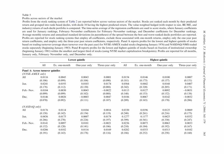
Table 5 reports the spread between deciles 10 and 1 within subsamples of stocks,both overall and broken down by season. The scoring system for generating thedeciles is identical to the scoring system used in the last table. Panel A employssubsamples based on turnover, defined as the number of shares traded per day as afraction of the number of shares outstanding, averaged over the prior 12 months.This share-normalized volume measure is employed by Lee and Swaminathan(2000), who show that it has a relatively low cross-sectional correlation with firmsize. Lee and Swaminathan (2000) examine NYSE-AMEX traded stocks and findthat momentum and subsequent three-year reversals are stronger among stocks withhigh turnover, mostly driven by the dismal performance of high turnover losers. In afootnote, Lee and Swaminathan (2000) also report that they replicated their resultswith NASDAQ-NMS firms from 1983 to 1996 and that, for these firms, thepredictive power of turnover for future returns appeared even stronger.

Trading volume is not comparable between stocks listed on NASDAQ and thoselisted on either the NYSE or AMEX exchanges. Due to the dealer system, eachNASDAQ trade is generally counted twice and sometimes more, exaggeratingtrading turnover relative to the traditional exchanges. Therefore, we separatelyreport results for NYSE/AMEX and NASDAQ stocks. The breakpoints for theturnover quintiles are exchange specific. In general, the investment strategies weformulate generate higher returns among high turnover stocks, consistent with Leeand Swaminathan (2000). However, the added profitability among high turnoverNASDAQ stocks is due to performance at the turn of the year. Among NASDAQ


ARTIC

LEIN

PRES

STable 5

Profits across sectors of the market

Profits from the stock ranking system of Table 2 are reported below across various sectors of the market. Stocks are ranked each month by their predicted

return and grouped into rank-based deciles, with decile 10 having the highest predicted return. The value-weighted hedged (with respect to size, BE/ME, and

industry) return of each decile portfolio is computed. The time-series average of the regression coefficients are used to score stocks, where January coefficients

are used for January rankings, February–November coefficients for February–November rankings, and December coefficients for December rankings.

Average monthly returns and annualized standard deviations (in parentheses) of the spread between the best and worst-ranked decile portfolios are reported.

Profits are reported for stock ranking systems that employ all coefficients, exclude those associated with one-month returns, employ only the one-year past

return coefficients, and employ only the three-year past return coefficients, respectively. Panel A reports profits for the lowest and highest quintile of stocks

based on trading turnover (average share turnover over the past year) for NYSE-AMEX traded stocks (beginning January 1976) and NASDAQ-NMS traded

stocks separately (beginning January 1983). Panel B reports profits for the lowest and highest quintile of stocks based on fraction of institutional ownership

(beginning January 1981) within the smallest and largest third of stocks (using NYSE market capitalization breakpoints). Profits are reported for all months,

January only, February–November only, and December only.

Lowest quintile Highest quintile

All Ex. one-month One-year only Three-year only All Ex. one-month One-year only Three-year only

Panel A: Across turnover quintiles

(NYSE-AMEX only)

All 0.0116 0.0043 0.0043 0.0001 0.0154 0.0146 0.0100 0.0007

(0.106) (0.099) (0.104) (0.090) (0.181) (0.175) (0.157) (0.151)

Jan. 0.0241 0.0193 0.0103 0.0174 0.0564 0.0442 0.0168 0.0407

(0.178) (0.112) (0.130) (0.088) (0.342) (0.320) (0.205) (0.171)

Feb.–Nov. 0.0104 0.0030 0.0043 �0.0022 0.0113 0.0127 0.0092 �0.0031

(0.099) (0.099) (0.102) (0.088) (0.148) (0.153) (0.152) (0.138)

Dec. 0.0146 0.0026 �0.0003 0.0047 0.0186 0.0067 0.0142 �0.0032

(0.070) (0.092) (0.111) (0.107) (0.209) (0.165) (0.170) (0.206)

(NASDAQ only)

All 0.0176 0.0114 0.0104 0.0016 0.0330 0.0196 0.0125 0.0069

(0.158) (0.142) (0.154) (0.119) (0.248) (0.261) (0.216) (0.175)

Jan. 0.0436 0.0175 0.0007 0.0174 0.1277 0.1177 0.0425 0.0352

(0.286) (0.270) (0.224) (0.197) (0.399) (0.541) (0.330) (0.247)

Feb.–Nov. 0.0141 0.0097 0.0101 �0.0021 0.0236 0.0075 0.0063 0.0033

(0.132) (0.120) (0.141) (0.106) (0.210) (0.184) (0.192) (0.167)

Dec. 0.0206 0.0182 0.0116 0.0169 0.0282 0.0353 0.0313 0.0102

(0.191) (0.143) (0.178) (0.116) (0.186) (0.252) (0.258) (0.160)

M.

Grin

bla

tt,T

.J.

Mo

sko

witz

/J

ou

rna

lo

fF

ina

ncia

lE

con

om

ics7

1(

20

04

)5

41

–5

79

565

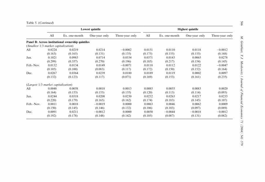
ARTIC

LEIN

PRES

STable 5. (Continued)

Lowest quintile Highest quintile


Panel B: Across institutional ownership quintiles

(Smallest 1/3 market capitalization)

All 0.0224 0.0219 0.0214 �0.0002 0.0151 0.0110 0.0118 �0.0012

(0.163) (0.165) (0.131) (0.135) (0.175) (0.155) (0.155) (0.168)

Jan. 0.1021 0.0983 0.0714 0.0534 0.0371 0.0143 0.0065 0.0278

(0.299) (0.357) (0.270) (0.196) (0.185) (0.217) (0.154) (0.145)

Feb.-Nov. 0.0132 0.0134 0.0149 �0.0071 0.0118 0.0112 0.0122 �0.0047

(0.105) (0.100) (0.083) (0.117) (0.172) (0.150) (0.152) (0.164)

Dec. 0.0267 0.0364 0.0239 0.0180 0.0189 0.0119 0.0002 0.0097

(0.132) (0.123) (0.117) (0.071) (0.169) (0.153) (0.161) (0.235)

(Largest 1/3 market capitalization)

All 0.0048 0.0058 0.0018 0.0013 0.0085 0.0055 0.0083 0.0020

(0.164) (0.153) (0.153) (0.135) (0.120) (0.113) (0.114) (0.093)

Jan. 0.0244 0.0318 0.0208 0.0230 0.0232 0.0263 0.0217 0.0235

(0.220) (0.179) (0.165) (0.162) (0.174) (0.183) (0.145) (0.107)

Feb.–Nov. 0.0011 0.0018 �0.0019 0.0000 0.0063 0.0046 0.0062 0.0009

(0.150) (0.145) (0.146) (0.132) (0.106) (0.103) (0.097) (0.089)

Dec. 0.0091 0.0211 �0.0012 0.0000 0.0050 �0.0044 �0.0018 �0.0012

(0.192) (0.178) (0.148) (0.142) (0.105) (0.087) (0.131) (0.082)

M.

Grin

bla

tt,T

.J.

Mo

sko

witz

/J

ou

rna

lo

fF

ina

ncia

lE

con

om

ics7

1(

20

04

)5

41

–5

79

566

firms, for instance, the enhanced profitability of one-year momentum by highturnover is entirely due to January and December, consistent with year-end tax-lossselling. In December, the high turnover momentum stocks outperform the lowturnover momentum stocks. In January the reverse is true, but our one-year strategybecomes a contrarian strategy at that point. Among NYSE-AMEX stocks, the one-year strategy is more profitable on high turnover than low turnover stocks fromFebruary to November. While this may imply that other factors besides tax-lossselling contribute to the results, it would be difficult for such a theory tosimultaneously explain why the reverse is true for NASDAQ stocks. Such a theorywould also have to explain why, even among NYSE/AMEX stocks, the degree towhich turnover enhances profitability is so much higher in December. Note also thatamong both NYSE/AMEX (as with NASDAQ stocks), the high turnover one-yearstrategy outperforms the low turnover strategy in January. Since the latter strategy iscontrarian in January, a low turnover momentum strategy should outperform a highturnover momentum strategy in January.

The salience of December and January to the enhanced profitability of thestrategies among high turnover stocks seems inconsistent with Lee andSwaminathan’s (2000) behavioral story of a ‘‘momentum life cycle.’’ This story,like most behavioral stories, should not exhibit seasonalities. While it is possible thatsome combination of tax-loss selling and behavioral finance theory could account forthe observed turnover/profitability pattern, the empirical research used to justifythese theories makes no attempt to take out a component of returns due to tax-losstrading. Our findings point to year-end tax-loss selling as a potential alternative tothe mysterious role played by turnover in the relation between past returns andexpected returns.

To further investigate the role of tax-motivated trading on these profits, Table 5Panel B studies the spread between value-weighted deciles 10 and 1 across quintilesbased on the fraction of a firm’s shares held by institutions, as reported by Standard& Poor’s, within the smallest and largest third of stocks. Due to data limitations, theanalysis here is from 1981 on. Firm size quintiles use NYSE breakpoints. If tax-motivated trades drive the relation between past and future returns, then theprofitability of our strategies should be strongest among firms with low institutionalownership, particularly in December and January. This is because individualinvestors are likely to be more concerned than institutions about capital gains taxes.

For small-cap stocks, for which tax-motivated trades are likely to have the greatestimpact on prices, Panel B suggests that low institutional ownership enhances theprofitability of the strategies. This is most evident in January and December, afinding that is consistent with the results in Sias and Starks (1997). However, withinthe largest quintile of stocks, institutional ownership does not appear to have thesame effect, even for January and December.

An alternative explanation for the contrasting findings is related to theobservation by Grinblatt et al. (1995) that mutual funds, which concentrate in largecap stocks, tend to follow momentum strategies. Thus, it is possible that large capstocks with large institutional ownership have more mutual fund investment than thesmall-cap stocks with large institutional investment. To the extent that momentum


represents underreaction to news, the behavior of this institutional class can reducethe rewards to momentum investing in the stocks favored by mutual funds.However, this alternative explanation for the negligible impact of institutionalownership on large cap stocks cannot account for the seasonalities observed.

The top and bottom halves of Panel B also indicate that the profitability of thethree most profitable investment strategies decreases with firm size. For example, inthe second column, which has low institutional ownership, a strategy generated byall coefficients except those associated with the past month earns 201 basis points permonth when applied to only the smallest quintile of stocks, but only 58 basis pointsper month when applied to the largest quintile, most of which is accounted for byJanuary and December.3 Hence, the stronger influence of past returns on expectedreturns for small stocks documented by Hong et al. (2000) is at least partly driven bya strong year-end seasonal. Such seasonal patterns are difficult to explain with Honget al.’s (2000) slow information diffusion theory. The stronger December persistenceand January bounceback among the smallest firms appears more consistent with tax-loss trading, since small stocks have more volatile prices (and therefore are morelikely to be big winners or losers) and are owned by a larger fraction of individualinvestors who face capital gains taxation. On the other hand, the stronger profits forsmall stocks during the rest of the year can be due to other factors, including slowinformation diffusion.

5.2. The influence of the tax regime

So far, we have hinted that the strong seasonal pattern in the profitability of thesetechnical trading strategies is driven by tax-motivated trades. Evidence on turnoverand institutional ownership is supportive of this conjecture. To test this moredirectly, we examine how tax regime shifts alter the profitability of our tradingstrategy.

Poterba and Weisbenner (2001) analyze how returns in the first few trading days ofJanuary vary with changes in the holding period definition of short- and long-termgains, as well as changes in the dollar limit on losses used to offset adjusted grossincome. In contrast to their study, we examine changes in the maximum capital gainstax rate and analyze both December and January returns. More importantly, ourfocus is entirely different. We analyze how tax regimes affect the profitability oftechnical trading strategies, whether they are applied to all stocks or subgroups ofstocks, like the small cap and low institutional holding categories, that are expectedto be particularly susceptible to tax-loss trading.

We measure the profitability of our value-weighted trading strategy (excludingone-month effects) for two subsamples. First, we analyze high tax years, which areyears or intervals of years at which the beginning year t has a maximum short-termcapital gains tax rate that is at least 20% higher than the average of the maximumrate in the two surrounding years, t � 1 and t þ 1: Then, we analyze low tax years,

ARTICLE IN PRESS

3Earlier drafts of this paper observed that similar size distinctions arise when the subsamples are based

only on firm size and extend to the entire sample period.


which are years or intervals of years at which the beginning year has a maximumshort-term capital gains tax rate that is at least 20% lower than the average of themaximum rate in the two surrounding years. Years that do not fall into either of the20% change categories share the same classification as the year immediately prior.By this rule, high tax years correspond to 1968–1969, 1972–1975, 1981, 1985–1986,1988–1999 and low tax years are all other years in our sample. In determiningwhether a particular January belongs to a high or low tax year, we assign therespective January to the year of its adjacent December. For example, January 1982is a high tax observation because 1981 is a high tax year.

To test whether differences across tax regimes affect strategy profitability, we runa time-series regression of the spread between the hedged returns of value-weighteddeciles 10 and 1, using the ranking system that excludes the past one-monthregressors, on dummy variables for high tax years, Januarys, Decembers, high taxJanuarys, and high tax Decembers. In this regression, the intercept represents thestrategy’s average profitability in low tax February–November months, and thecoefficients on the five dummy variables represent the marginal effect on strategyprofitability of various types of months.

Table 6 Panel A reports the coefficients and t-statistics from this regression. Themost striking aspect of the regression is that only the high tax January and high taxDecember coefficients are significant. The lack of statistically significant averageprofits from February to November and turn-of-the-year seasonals in low tax yearsis also rather surprising.

The insignificance of three of the five dummy coefficients in Panel A implies onlythat the marginal effect of the associated variables is insignificant. Profits earned inthe months represented by the insignificant dummy variables could still significantlydiffer from zero. However, analyzing this issue directly, we find that only the hightax-year profits significantly differ from zero. This is rather obvious in December,where the low tax profits are only �27 basis points per month (obtained bysubtracting the December coefficient from the constant). However, even the low tax-year January profit of 162 basis points (the sum of the constant and the coefficient onthe January dummy), although economically notable, does not significantly differfrom zero when earned over only 12 Januarys (t ¼ 1:31). Moreover, the averagemonthly profit over all months in the low tax regime, 37 basis points, is alsoinsignificant (t ¼ 1:08). By contrast, average February–November profits in high taxyears are 75 basis points per month, which significantly differs from zero (t ¼ 2:63).This high tax-year profit increases by 362 basis points in the high tax Januarys andby 451 basis points in the high tax Decembers. Hence, not only do profits from thestrategy substantially increase from insignificant to significant in high tax years, butthere is a pronounced seasonality to the profits that is not present in the low taxyears.

The pattern observed in Table 6 Panel A is consistent with tax-loss selling as animportant driver of the strategy’s profitability. Even the significant profits fromFebruary through November of high tax years could be generated by a steadilyincreasing supply of losing stocks for sale that reaches a peak in December.However, if the profitability pattern across tax regimes is truly due to tax-loss selling,


ARTIC

LEIN

PRES

S

Table 6

How does tax-loss trading affect the relation between past and expected returns?

Profits are reported from the stock ranking system of Table 2 during different tax regimes based on the maximum short-term capital gains tax rate. Stocks are

ranked each month by their predicted return and grouped into rank-based deciles, with decile 10 having the highest predicted return. The value-weighted

hedged (with respect to size, BE/ME, and industry) return of each decile portfolio is computed. The time-series average of the August 1966 to July 1995

regression coefficients (excluding one-month regressors) are used to score stocks, where January coefficients are used for January rankings, February–

November coefficients for February–November rankings, and December coefficients for December rankings. Panel A conducts formal tests of tax regime

effects by reporting time-series regression coefficients of the profits on seasonal dummies, tax regime dummies, and their interactions. t-statistics on the

coefficients are reported in parentheses. Since tax-loss selling should predominantly apply to past losing stocks and since the trading strategy shorts past

losers in December (due to continuation) and buys past losers in January (due to reversals), profits are reported separately for decile 1 in December and decile

10 in January in Panels B and C, respectively. Average monthly returns and annualized standard deviations (in parentheses) of the worst and best- ranked

decile portfolios are reported for December and January, respectively, across the two tax regimes. These profits are reported for the smallest and largest

quintile of stocks (using NYSE breakpoints), and lowest and highest institutional ownership (%IO) quintile of stocks among the smallest and largest third of

stocks over the period August 1966 to December 1999. The high tax years are 1968–1969, 1981, 1972–1975, 1985–1986, and 1988–1999. The remaining years

are low tax years.

Profits: August 1966 to December 1999

Strategy: Exclude one-month regressors

Panel A: Time-series regression

Constant High tax High tax Jan. High tax Dec. Jan. Dec.

All stocks 0.0033 0.0042 0:0364�� 0:0451�� 0.0129 �0:0068(0.88) (0.88) (2.39) (3.30) (1.00) ð�0:55Þ

Smallest 1/3 size Largest 1/3 size

Smallest size Largest size Lowest %IO Highest %IO Lowest %IO Highest %IO

quintile quintile quintile quintile quintile quintile

M.

Grin

bla

tt,T

.J.

Mo

sko

witz

/J

ou

rna

lo

fF

ina

ncia

lE

con

om

ics7

1(

20

04

)5

41

–5

79

570

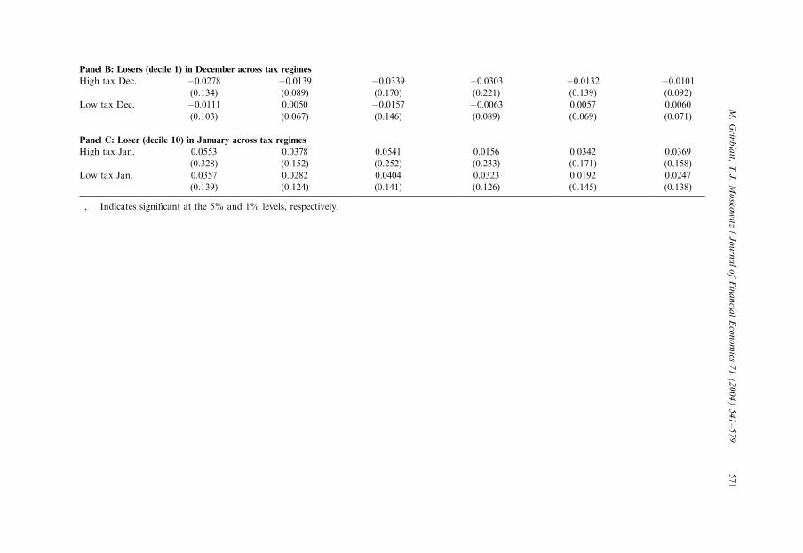
ARTIC

LEIN

PRES

SPanel B: Losers (decile 1) in December across tax regimes

High tax Dec. �0:0278 �0:0139 �0:0339 �0:0303 �0:0132 �0:0101(0.134) (0.089) (0.170) (0.221) (0.139) (0.092)

Low tax Dec. �0:0111 0:0050 �0:0157 �0:0063 0.0057 0.0060

(0.103) (0.067) (0.146) (0.089) (0.069) (0.071)

Panel C: Loser (decile 10) in January across tax regimes

High tax Jan. 0.0553 0.0378 0.0541 0.0156 0.0342 0.0369

(0.328) (0.152) (0.252) (0.233) (0.171) (0.158)

Low tax Jan. 0.0357 0.0282 0.0404 0.0323 0.0192 0.0247

(0.139) (0.124) (0.141) (0.126) (0.145) (0.138)

�; ��Indicates significant at the 5% and 1% levels, respectively.

M.

Grin

bla

tt,T

.J.

Mo

sko

witz

/J

ou

rna

lo

fF

ina

ncia

lE

con

om

ics7

1(

20

04

)5

41

–5

79

571

it should show up most strongly among the decile of losing stocks. Because we areexcluding the past one-month in formulating the strategy, this corresponds to decile1 in December and to decile 10 in January. Moreover, this turn-of-the-year patternacross tax regimes should exhibit enhanced profits for those stocks that are mostlikely held by taxable investors. These would be small-cap stocks with lowinstitutional ownership.

Panels B and C of Table 6 report the December and January hedged returns oflosing stocks. Panel B reports the hedged December returns of the decile 1 portfoliowithin six subcategories of stocks and across the two tax regimes. Panel C reports theanalogous January hedged returns of the decile 10 portfolios. The six subcategoriesconsist of three matching category pairs: smallest and largest quintile of stocks,lowest and highest institutional ownership quintile within the smallest third ofstocks, and lowest and highest institutional ownership quintile within the largestthird of stocks. The results in these two panels are consistent with tax-loss sellingbeing an important driver of the temporal link between stock returns.

In Table 6 Panel B, the decile 1 stocks (losers) exhibit negative hedged returns inhigh tax Decembers. These hedged returns are substantially lower than the hedgedreturns in low tax Decembers, across all categories. In Panel C, the decile 10 stockshave sizable positive hedged returns in high tax Januarys. In all but one case theyexceed their low tax counterparts. The exception is a high institutional ownershipcategory which should not be particularly tax rate sensitive.

The tax hypothesis also seems supported by comparisons made across categories.In Table 6 Panel B, the high tax December hedged returns of decile 10 are negativefor each category of stocks, but substantially more negative for the less taxableownership category within each of the three pairings. In low tax Decembers, themore taxable ownership category in each of the three pairings has lower hedgedreturns, but many of the hedged returns are positive. Among large cap stocks,institutional ownership only accounts for a three basis point difference inDecember.

In Table 6 Panel C, every category of stock ownership has positive decile 10hedged returns. However, in both high and low tax Januarys, it is the taxablecategory within each of the two small-cap pairings that has the more positive returns.Among large-cap stocks, institutional ownership appears to have the reverse(although negligible) effect on profitability. Thus, it appears as if institutionalownership may not be related to tax-loss selling among value-weighted portfolios oflarge-cap stocks. This would not be surprising if tax-loss selling accounts for ourfindings.

6. Transaction costs and out-of-sample results

Finally, given the large profits associated with our trading strategies based onconsistency and tax-related effects, we assess whether the profits generated fromthese strategies could have persisted because of substantial trading frictions or are abyproduct of data snooping.


6.1. Turnover for trading strategies and transaction costs

An investor trying to exploit the strategies described above would need to accountfor trading costs in deciding whether to pursue these strategies. The investor wouldwant to avoid or downweight stocks with particularly high trading costs, notablystocks with low prices and small market capitalizations, and would be moreinterested in value- than equal-weighted portfolios. The investor also might avoidemploying information from the past one-month return due to potential market-microstructure effects.

In our case, restricting the value-weighted portfolios formed in Table 3 to above$5 stocks is fairly innocuous. For comparison purposes, the left-hand side of Panel Aof Table 7 summarizes the same information in Table 3, broken down by season. Theleft-hand side of Table 7 Panel B repeats the analysis in Panel A, but focusesexclusively on stocks with prices above $5 at the beginning of the month. As can beseen from the table, the average spread between value-weighted deciles 10 and 1generally declines, but only slightly. In going from Panels A to B, the decline is fourbasis points per month for the overall strategy, 11 basis points for the strategy thatexcludes the prior month, and one basis point with the three-year strategy. With theone-year strategy, it actually increases from 71 basis points per month when using allstocks to 77 basis points per month when using just the stocks with share pricesexceeding $5.

It is instructive to focus on the second column in Panel B in trying to assesswhether this is a viable strategy for an investor concerned about trading costs. While100 basis points per month is impressive, the turnover of the strategy is large. In ourfinal and particularly volatile year, 1999, turnover (dollar-buys plus dollar-sells perdollar invested) on the long side of the strategy (decile 10) is 38.86% per month,while that on the short side (decile 1) is 63.75% per month. Trading costs of about1% are approximately the breakeven costs for this strategy. On the other hand,because of value weighting, the typical dollar invested in a long or a short position isin a stock that is in the 86th percentile of market capitalization (for both the long andthe short positions). These stocks have substantially lower trading costs than theaverage stock. Moreover, the information we use in formulating the strategy thatexcludes the past month is at least a month old. Hence, there is no urgency to thetrades, allowing such trades to be split into smaller sizes and executed over a periodof days or perhaps even weeks.

A recent study by a practitioner expert, Wayne Wagner, (www.plexusgroup.com)has estimated that for large cap stocks, a cost of about 0.32% reflects marketimpact and brokerage commission for trades, while 0.55% covers a smallercap trade. Since the introduction of decimalization and Internet commissionswere not accounted for in this study, these costs may now be even lower. Forearlier periods, when institutional brokerage commissions accounted for 20 to 30basis points of trading costs, depending on share price, the findings in Keimand Madhavan (1997) support the notion that trading costs would be far less than100 basis points for a value-weighted strategy restricted to stocks with share pricesabove $5.


http://www.plexusgroup.com

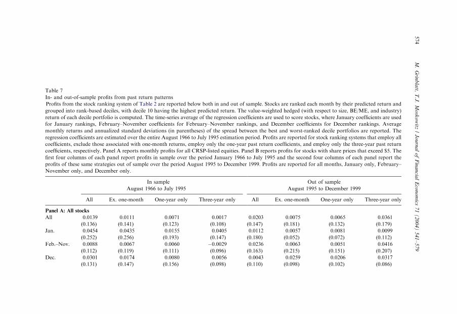
ARTIC

LEIN

PRES

S

Table 7

In- and out-of-sample profits from past return patterns

Profits from the stock ranking system of Table 2 are reported below both in and out of sample. Stocks are ranked each month by their predicted return and

grouped into rank-based deciles, with decile 10 having the highest predicted return. The value-weighted hedged (with respect to size, BE/ME, and industry)

return of each decile portfolio is computed. The time-series average of the regression coefficients are used to score stocks, where January coefficients are used

for January rankings, February–November coefficients for February–November rankings, and December coefficients for December rankings. Average

monthly returns and annualized standard deviations (in parentheses) of the spread between the best and worst-ranked decile portfolios are reported. The

regression coefficients are estimated over the entire August 1966 to July 1995 estimation period. Profits are reported for stock ranking systems that employ all

coefficients, exclude those associated with one-month returns, employ only the one-year past return coefficients, and employ only the three-year past return

coefficients, respectively. Panel A reports monthly profits for all CRSP-listed equities. Panel B reports profits for stocks with share prices that exceed $5. The

first four columns of each panel report profits in sample over the period January 1966 to July 1995 and the second four columns of each panel report the

profits of these same strategies out of sample over the period August 1995 to December 1999. Profits are reported for all months, January only, February–

November only, and December only.

In sample Out of sample

August 1966 to July 1995 August 1995 to December 1999


Panel A: All stocks

All 0.0139 0.0111 0.0071 0.0017 0.0203 0.0075 0.0065 0.0361

(0.136) (0.141) (0.123) (0.108) (0.147) (0.181) (0.132) (0.179)

Jan. 0.0454 0.0435 0.0155 0.0405 0.0112 0.0057 0.0081 0.0099

(0.252) (0.256) (0.193) (0.147) (0.180) (0.052) (0.072) (0.112)

Feb.–Nov. 0.0088 0.0067 0.0060 �0.0029 0.0236 0.0063 0.0051 0.0416

(0.112) (0.119) (0.111) (0.096) (0.163) (0.215) (0.151) (0.207)

Dec. 0.0301 0.0174 0.0080 0.0056 0.0043 0.0259 0.0206 0.0317

(0.131) (0.147) (0.156) (0.098) (0.110) (0.098) (0.102) (0.086)

M.

Grin

bla

tt,T

.J.

Mo

sko

witz

/J

ou

rna

lo

fF

ina

ncia

lE

con

om

ics7

1(

20

04

)5

41

–5

79

574

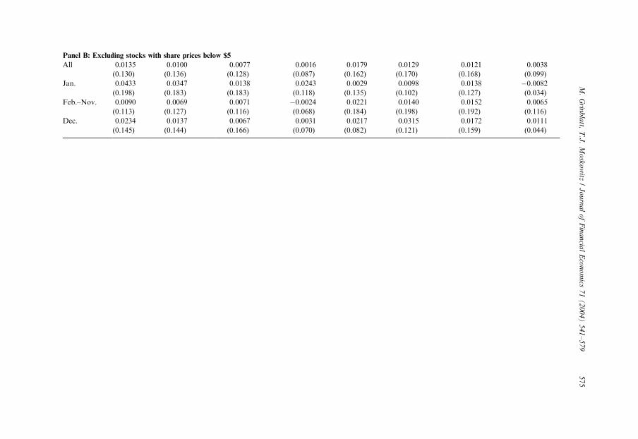
ARTIC

LEIN

PRES

SPanel B: Excluding stocks with share prices below $5

All 0.0135 0.0100 0.0077 0.0016 0.0179 0.0129 0.0121 0.0038

(0.130) (0.136) (0.128) (0.087) (0.162) (0.170) (0.168) (0.099)

Jan. 0.0433 0.0347 0.0138 0.0243 0.0029 0.0098 0.0138 �0.0082

(0.198) (0.183) (0.183) (0.118) (0.135) (0.102) (0.127) (0.034)

Feb.–Nov. 0.0090 0.0069 0.0071 �0.0024 0.0221 0.0140 0.0152 0.0065

(0.113) (0.127) (0.116) (0.068) (0.184) (0.198) (0.192) (0.116)

Dec. 0.0234 0.0137 0.0067 0.0031 0.0217 0.0315 0.0172 0.0111

(0.145) (0.144) (0.166) (0.070) (0.082) (0.121) (0.159) (0.044)

M.

Grin

bla

tt,T

.J.

Mo

sko

witz

/J

ou

rna

lo

fF

ina

ncia

lE

con

om

ics7

1(

20

04

)5

41

–5

79

575

A significant component of the turnover in the strategy comes from shortingdecile 1. Short sales of the stocks in decile 1, however, are not necessary to earnsubstantial profits relative to the benchmark. The profits for the long side of thestrategy (decile 10) net of benchmark portfolio returns are 66 basis points per month.Hence, even if short-sales restrictions were costly, and D’Avolio (2002) and Reed(2002) find that for most stocks they are not, there still are substantial rents that canbe earned from a long strategy that beats a similar book-to-market, size, andindustry-matched benchmark. The 66 basis points per month abnormal return frombuying decile 10 would only be wiped out by one-way transaction costs of at least1.70%, which could be almost an order of magnitude too high for value-weightedportfolios.

6.2. Out-of-sample results

The scoring system that generates the ranks for the stocks is derived from the samesample of data used to assess profitability. Moreover, the specification for thescoring system employs variables known to be related to average returns fromprevious studies. Sullivan et al. (1999) suggest that calendar effects in stock returns,like the anomalous January effect, can be generated purely by data snooping. If thesuccess of our specification of the regressors was the product of an intensive searchfor the most marketable (or publishable) trading strategy using past literature as aguide, the results obtained here would not hold for the five years of additional datathat became available after the first draft of this paper formulated this tradingstrategy.

The right-hand side of Table 7 reports the same profitability information as itsleft-hand side counterpart. It uses the same ranking strategy based on the samecoefficients as that used on the left-hand side. Despite the handicap of being entirelyout-of-sample, the spread in the hedged returns of the value-weighted deciles is eitherabout the same or is larger than it was in sample. For example, the all strategy isabout 64 basis points per month more profitable in the out-of-sample period, August1995–December 1999, as in the in-sample period. While not all of the out-of-samplenumbers exceed their in-sample counterparts, most are economically significant andof similar magnitude. This suggests that the observed structural relation betweenpast and future returns is relatively stable and is unlikely to be a product of datasnooping.

7. Conclusion

The past pattern of returns seems to matter as much as the magnitude of the pastreturn for the cross-section of expected returns. Most notably, we find thatconsistency of past winning stocks has a substantial impact on the cross-section ofreturns. In cross-sectional regressions, the marginal impact of consistent winners atall horizons is positively related to future average returns. Almost all of theconsistent winners’ coefficients are statistically significant. Moreover, being a


consistent winner is economically important. For the typical firm, being a consistentwinner can double the return premium associated with a firm belonging to the topmomentum decile.

Being a consistent loser appears to be irrelevant to the cross-section of returns. Wecan only speculate about the reasons for this. For example, tax-loss selling is likely toplay a larger role for consistent losers than consistent winners. It is possible that tax-loss selling is masking or offsetting whatever behavioral phenomenon contributes toa consistency effect in stock returns.

Although numerous studies attempt to analyze the tax-loss selling hypothesis,most focus on stock returns in January and do not examine variations in the tax codeor the role played by tax-loss selling in the profitability of momentum and reversalstrategies. We show that there are strong December effects in stock returns.Moreover, our argument that these seasonalities are related to tax-loss trading isbuttressed by our analysis of how tax regimes affect the relation between past andexpected returns. We find statistically significant profits from technical tradingstrategies only in high tax regimes, including the strong seasonal effects.Furthermore, the subcategories of stocks on which these technical trading strategieswork best (e.g., small, low institutional ownership stocks) are also those mostsusceptible to tax-loss trading.

Finally, we examine these novel findings in the context of recent behavioraltheories for past return predictability. Current theory is challenged by many of theresults we uncover. For instance, we find that at least part of the intermediate-termmomentum and long-term reversal effects evolve independently. The fact that thelong-term reversal effect appears only in January, yet significant momentum existsoutside of January, appears inconsistent with these effects resulting from the sameinvestor behavior, as suggested by recent theory. The strongest link seems to bedriven by end-of-year tax-loss selling. Certainly, future theory should consider therelevance and importance of both consistency and seasonal effects.

References

Ahn, D.H., Boudoukh, J., Richardson, M., Whitelaw, R., 2000. Behavioralize this! International evidence

on autocorrelation patterns of stock index and futures returns. Unpublished working paper, New York

University.

Asness, C.S., 1995. The power of past stock returns to explain future stock returns, Unpublished working

paper, Goldman Sachs Asset Management, New York, NY.

Ball, R., Kothari, S.P., 1989. Nonstationary expected returns: implications for tests of market efficiency

and serial correlation in returns. Journal of Financial Economics 25, 51–74.

Bansal, R., Ditmar, R., Lundblad, C., 2002. Consumption, dividends, and the cross-section of equity

returns. Unpublished working paper, Duke University.

Barberis, N., Shleifer, A., Vishny, R., 1998. A model of investor sentiment. Journal of Financial

Economics 49, 307–343.

Berges, A., McConnell, J.J., Schlarbaum, G., 1984. The turn of the year in Canada. Journal of Finance 39,

185–192.

Berk, J., Green, R., Naik, V., 1999. Optimal investment, growth options, and security returns. Journal of

Finance 54, 1553–1607.


Boudoukh, J., Richardson, M., Whitelaw, R., 1994. A tale of three schools: insights on auto correlations

of short-horizon stock returns. Review of Financial Studies 7, 539–573.

Carhart, M., 1997. On persistence in mutual fund performance. Journal of Finance 52, 57–82.

Chan, K.C., 1986. Can tax loss selling explain the January season in stock returns? Journal of Finance 41,

1115–1128.

Chan, K.C., 1988. On the contrarian investment strategy. Journal of Business 61, 147–163.

Chopra, N., Lakonishok, J., Ritter, J.R., 1992. Measuring abnormal performance: do stocks overreact?

Journal of Financial Economics 31, 235–268.

Chordia, T., Shivakumar, L., 2002. Momentum, business cycle, and time-varying expected returns.

Journal of Finance 57, 985–1019.

Conrad, J., Kaul, G., 1989. Mean reversion in short-horizon expected returns. Review of Financial Studies

2, 225–240.

Conrad, J., Kaul, G., 1998. An anatomy of trading strategies. Review of Financial Studies 11, 489–520.

Constantinides, G., 1984. Optimal stock trading with personal taxes. Journal of Financial Economics 13,

65–89.

Daniel, K., Titman, S., 1997. Evidence on the characteristics of cross-sectional variation in common stock

returns. Journal of Finance 52, 1–34.

Daniel, K., Hirshleifer, D., Subrahmanyam, A., 1998. Investor psychology and security market under- and

over-reactions. Journal of Finance 53, 1839–1886.

D’Avolio, G., 2002. The market for borrowing stock. Journal of Financial Economics 66, 271–306.

DeBondt, W.F.M., Thaler, R., 1985. Does the stock market overreact? Journal of Finance 40, 793–808.

DeBondt, W.F.M., Thaler, R., 1987. Further evidence on investor over-reaction and stock market

seasonality. Journal of Finance 42, 557–581.

Dyl, E., 1977. Capital gains taxation and year-end stock market behavior. Journal of Finance 32, 165–175.

Dyl, E., Maberly, E., 1992. Odd-lot transactions around the turn of the year and the January effect.

Journal of Financial and Quantitative Analysis 27, 591–604.

Fama, E.F., French, K.R., 1992. The cross-section of expected stock returns. Journal of Finance 47, 427–

465.

Fama, E.F., French, K.R., 1996. Multifactor explanations of asset pricing anomalies. Journal of Finance

51, 55–84.

Fama, E.F., MacBeth, J., 1973. Risk, return, and equilibrium: empirical tests. Journal of Political

Economy 71, 607–636.

Grinblatt, M., Han, B., 2002. The disposition effect and momentum. Unpublished working paper, UCLA,

Anderson School.

Grinblatt, M., Keloharju, M., 2001. What makes investors trade? Journal of Finance 56, 589–616.

Grinblatt, M., Keloharju, M., 2003. Tax-loss trading and wash sales. Journal of Financial Economics,

Article in Press.

Grinblatt, M., Titman, S., Wermers, R., 1995. Momentum investment strategies, portfolio performance,

and herding: a study of mutual fund behavior. American Economic Review 85, 1088–1105.

Grundy, B.D., Martin, J.S., 2001. Understanding the nature of the risks and the source of the rewards to

momentum investing. Review of Financial Studies 14, 29–78.

Hong, H., Stein, J.C., 1999. A unified theory of underreaction, momentum trading, and overreaction in

asset markets. Journal of Finance 54, 2143–2184.

Hong, H., Lim, T., Stein, J.C., 2000. Bad news travels slowly: size, analyst coverage, and the profitability

of momentum strategies. Journal of Finance 55, 265–296.

Hvidkjaer, S., 2001. A trade-based analysis of momentum. Unpublished working paper, University of

Maryland.

Jegadeesh, N., 1990. Evidence of predictable behavior of security returns. Journal of Finance 45, 881–898.

Jegadeesh, N., Titman, S., 1993. Returns to buying winners and selling losers: implications for stock

market efficiency. Journal of Finance 48, 65–91.

Jegadeesh, N., Titman, S., 1995. Short horizon return reversals and the bid–ask spread. Journal of

Financial Intermediation 4, 116–132.


Jegadeesh, N., Titman, S., 2001. Profitability of momentum strategies: an examination of alternative

explanations. Journal of Finance 56, 699–720.

Kaul, G., Nimalendran, M., 1990. Price reversals: bid–ask errors or market overreaction? Journal of

Financial Economics 28, 67–83.

Keim, D., 1983. Size related anomalies and stock return seasonality: further empirical evidence. Journal of

Financial Economics 12, 13–32.

Keim, D., 1989. Trading patterns, bid–ask spreads, and estimated security returns: the case of common

stock at calendar turning points. Journal of Financial Economics 25, 75–97.

Keim, D., Madhavan, A., 1997. Transactions costs and investment style: an inter-exchange analysis of

institutional equity trades. Journal of Financial Economics 46, 265–292.

Lakonishok, J., Smidt, S., 1988. Are seasonal anomalies real? A ninety year perspective. Review of

Financial Studies 3, 257–280.

Lee, C., Swaminathan, B., 2000. Price momentum and trading volume. Journal of Finance 55, 2017–2070.

Lehman, B., 1990. Fads, martingales, and market efficiency. Quarterly Journal of Economics 105, 1–28.

Lo, A.W., MacKinlay, A.C., 1988. Stock market prices do not follow random walks: evidence from a

simple specification test. Review of Financial Studies 1, 41–66.

Moskowitz, T.J., Grinblatt, M., 1999. Do industries explain momentum? Journal of Finance 54,

1249–1290.

Pechman, J.A., 1987. Federal Tax Policy, 5th Edition. Brookings Institution Press, Washington, DC.

Poterba, J.M., Weisbenner, S.J., 2001. Capital gains tax rules, tax loss trading, and turn-of-the-year

returns. Journal of Finance 56, 353–368.

Reed, A., 2002. Costly short-selling and stock price adjustment to earnings announcements. Unpublished

working paper, University of North Carolina, Chapel Hill.

Reinganum, M., 1983. The anomalous stock market behavior of small firms in January: empirical tests for

tax-loss selling effects. Journal of Financial Economics 12, 89–104.

Reinganum, M., Shapiro, A., 1987. Taxes and stock return seasonality: evidence from the London Stock

Exchange. Journal of Business 60, 281–295.

Roll, R., 1983. Vas ist das? The turn-of-the-year effect and the return premia of small firms. Journal of

Portfolio Management 9, 18–28.

Rouwenhorst, K.G., 1998. International momentum strategies. Journal of Finance 53, 267–284.

Sias, R.W., Starks, L.T., 1997. Institutions and individuals at the turn-of-the-year. Journal of Finance 52,

1543–1562.

Sullivan, R., Timmermann, A., White, H., 1999. Data snooping, technical trading rule performance, and

the bootstrap. Journal of Finance 54, 1647–1692.

Watkins, B., 2002. Does consistency predict returns? Unpublished working paper, Syracuse University.

Willan, R.M., 1994. Income Taxes: Concise History and Primer. Claitor’s Publishing Division, Baton

Rouge, LA.


Documents

Predicting stock price movements from past returns: the - Faculty