Electronic copy available at: http://ssrn.com/abstract=1787285

Predicting Market Returns Using Aggregate Implied Cost of CapitalI

Yan Lia,∗, David Ngb, Bhaskaran Swaminathanc

aDepartment of Finance, Fox School of Business, Temple University, Philadelphia, PA 19122bDyson School of Applied Economics and Management, Cornell University, Ithaca, NY 14853

cLSV Asset Management, 155 North Wacker Dr., Chicago, IL 60606

Abstract

Theoretically, the implied cost of capital (ICC ) is a good proxy for time-varying expected returns.

We find that aggregate ICC strongly predicts future excess market returns at horizons ranging from

one month to four years. This predictive power persists even in the presence of popular valuation

ratios and business cycle variables, both in-sample and out-of-sample, and is robust to alternative

implementations. We also find that ICC s of size and B/M portfolios predict corresponding portfolio

returns.

Keywords: Implied Cost of Capital, Market Predictability, Valuation Ratios

JEL: G12

IThe original version of the paper was circulated with the title “Implied Cost of Capital and the Predictability ofMarket Returns ”. We thank an anonymous referee, Sudipta Basu, Hendrik Bessembinder, Robert Engle, Frank Diebold,Stephan Dieckmann, Wayne Ferson, George Gao, Hui Guo, Jingzhi Huang, Ming Huang, Kewei Hou, Andrew Karolyi,Dana Kiku, Charles Lee, Xi Li, Maureen O’Hara, Robert J. Hodrick, Roger K. Loh, Lilian Ng, Matt Pritsker, DavidReeb, Michael Roberts, Oleg Rytchkov, Thomas Sargent, G. William Schwert (the editor), Steve Sharpe, Nick Souleles,Robert F. Stambaugh, Ramu Thiagarajan, Amir Yaron, Yuzhao Zhang, and seminar participants at American EconomicAssociation Annual Meeting, China Europe International Business School, Cornell University, Journal of InvestmentManagement Conference, Peking University, Singapore Management University, the Federal Reserve Board, ShanghaiAdvanced Institute of Finance, Temple University, University of Hong Kong, the Wharton School, and Xiamen Universityfor helpful comments. Any errors are our own.

∗Corresponding authorEmail addresses: liyanlpl@temple.edu (Yan Li), dtn4@cornell.edu (David Ng), swami@lsvasset.com

(Bhaskaran Swaminathan)

Preprint submitted to Elsevier March 18, 2013

Electronic copy available at: http://ssrn.com/abstract=1787285

Predicting Market Returns Using Aggregate Implied Cost of Capital

Abstract

Theoretically, the implied cost of capital (ICC ) is a good proxy for time-varying expected returns.

We find that aggregate ICC strongly predicts future excess market returns at horizons ranging from

one month to four years. This predictive power persists even in the presence of popular valuation

ratios and business cycle variables, both in-sample and out-of-sample, and is robust to alternative

implementations. We also find that ICC s of size and B/M portfolios predict corresponding portfolio

returns.

Keywords: Implied Cost of Capital, Market Predictability, Valuation Ratios

JEL: G12

Preprint submitted to Elsevier March 18, 2013

1. Introduction

The issue of return predictability is of great interest to academics and practitioners. Traditional

academic literature has focused on the usefulness of valuation ratios such as dividend-to-price ratio,

book-to-market ratio, earnings-to-price ratio and payout yield in predicting future returns (e.g., Fama

and Schwert (1977), Campbell (1987), Campbell and Shiller (1988), Fama and French (1988a), Kothari

and Shanken (1997), and Boudoukh et al. (2007)). Various business cycle variables have also been

proposed as forecasting variables (e.g., Campbell (1987) and Fama and French (1989)). Whether

return predictability exists is still an on-going debate. For instance, Ang and Bekaert (2007) find that

the dividend yield does not have any long horizon predictive power once standard errors that are less

biased in small samples are used to conduct statistical inference. Boudoukh, Richardson, and Whitelaw

(2008) show that long horizon tests are not more powerful than short horizon tests, and find that only

net payout yield and net equity issuance have the ability to predict returns under joint predictability

tests. Cochrane (2008), however, argues that the absence of dividend growth predictability is stronger

evidence for return predictability than the presence of return predictability itself. Welch and Goyal

(2008) question the existence on stock return predictability using out of sample tests, but subsequent

studies by Rapach, Strauss, and Zhou (2010), Henkel, Martin, and Nardari (2011), and Dangl and

Halling (2012) re-affirm the evidence on predictability. Our paper strengthens the empirical evidence

on predictability by introducing a new predictor, the aggregate implied cost of capital (ICC ), that

performs better than existing forecasting variables.

The ICC is estimated as the expected return that equates a stock’s current price to the present

value of its expected future free cash flows where, empirically, the free cash flows are estimated using

a combination of short-term analyst earnings forecasts, long-term growth rates projected from the

short-term forecasts, and historical payout ratios. The ICC has historically been used to estimate

the unconditional equity premium, compute individual firm cost of equity, and address various other

cross-sectional asset pricing issues.1 Pastor, Sinha, and Swaminathan (2008) use the ICC in a time-

series setting and show theoretically that the aggregate ICC is a good proxy for time-varying expected

returns. They use the aggregate ICC to examine the inter-temporal asset pricing relationship between

expected returns and volatility, and find a positive relationship between the two. If the aggregate ICC

is a good proxy of time-varying expected returns, it should also predict future market returns. In

addition, since the ICC is based on a theoretically justifiable valuation model that takes into account

future growth opportunities, it is of interest to know whether ICC performs better in predicting future

1There is a large literature on the ICC. See Richardson, Tuna, and Wysocki (2010) for a literature review.

2

returns than traditional valuation ratios such as dividend yield and earnings yield. These are the issues

we examine in this paper.

Our paper also has potential implications for the ICC literature. A key requirement for the

usefulness of the ICC is to show that the ICC positively predicts future returns. Existing cross-

sectional studies on the ICC have been unable to conclusively establish such a positive relationship

(see Easton and Monahan (2005), Richardson, Tuna, and Wysocki (2010), and Hou, van Dijk, and

Zhang (2012)). The absence of such evidence, however, might be due more to the noise in computing

individual firm ICC s under the various methods used in the literature than to any theoretical problems

with the ICC approach (see Lee, So, and Wang (2010)). The aggregate ICC is likely to be less noisy

(since it is computed by averaging individual firm ICC s) and, therefore, might be more successful in

predicting future returns.

We estimate the aggregate ICC by value-weighting the ICC s of firms in the S&P 500 index each

month. We then subtract the one-month T-bill yield from the aggregate ICC to compute the excess

ICC (the implied risk premium) and use it to forecast future excess market returns. For the sake

of exposition, however, we refer to excess ICC as ICC throughout the paper. We use the standard

forecasting regression methodology to examine the predictive power of the ICC. Our results, based on

monthly data from January 1977 to December 2011, show that the ICC is a strong predictor of future

market returns over the next four years, with adjusted R2 ranging from 7% at the 1-year horizon to

31% at the 4-year horizon. Specifically, high ICC predicts high returns. The predictive power of the

ICC remains strong even after we control for widely-used valuation ratios such as the earnings-to-price

ratio, dividend-to-price ratio, book-to-market ratio, and payout yield, and business cycle variables such

as the term spread, default spread, long-term government bond yield, and the T-bill rate. In contrast,

valuation ratios and business cycle variables perform poorly during this sample period.

Our results are robust to a host of other checks. Since long horizon forecasting regressions are rife

with small sample biases, we use Monte Carlo simulations to assess the statistical significance of our

regression statistics (e.g., Hodrick (1992) and Stambaugh (1999)). The predictive power of the ICC

remains strong even under these stringent simulated p-values. Our results also hold when we construct

the ICC in alternative ways and under reasonable perturbations to the forecasting horizons of the free

cash flow model.

We contend above that the aggregate ICC is likely to be less noisy since it is computed by averaging

the firm level ICC s thereby reducing the estimation errors present in firm level ICC s. Indeed, we find

that the aggregate ICC is a strong time-series predictor of future market returns in contrast to mixed

evidence on the cross-sectional predictive power of individual firm ICC s. If aggregation helps reduce

3

estimation errors at the aggregate market level, it should also work at the portfolio level. Consistent

with this intuition, we find that the ICC s of size and book-to-market portfolios strongly predict

corresponding size and B/M portfolio returns.

Recently, out-of-sample forecasting tests have received much attention in the literature (see Welch

and Goyal (2008)). We perform a variety of out-of-sample tests and find that the ICC is also an

excellent out-of-sample predictor of future market returns. During 1998-2011, the period we use to

evaluate out-of-sample performance, the ICC delivers higher out-of-sample R2 than its competitors,

and provides positive utility gains of more than 4% per year to a mean-variance investor. Since

Rapach, Strauss, and Zhou (2010) argue that it is important to combine individual predictors in the

out-of-sample setting, we conduct a forecasting encompassing test, which provides strong evidence

that the ICC contains distinct information above and beyond that contained in existing predictors.

The key reason for the ICC ’s superior performance is that the ICC is estimated from a theoretically

justifiable discounted cash flow valuation model that takes into account future growth opportunities

that are ignored by traditional valuation ratios. Overall, our paper makes three contributions to the

literature: (a) we provide strong evidence in favor of aggregate stock market predictability, (b) we

introduce a new forecasting variable, the ICC, which forecasts future returns better than existing

forecasting variables, both in-sample and out-of-sample, and (c) we also validate the usefulness of the

ICC approach by showing that the ICC can positively predict future returns.

Our paper proceeds as follows. We describe the methodology for constructing the aggregate ICC

in Section 2. Section 3 provides the data source and summary statistics. Section 4 and Section 5

present in-sample and out-of-sample return predictions, respectively. Section 6 concludes the paper.

2. Empirical Methodology

In this section, we first explain why the implied cost of capital is a good proxy for expected returns.

We then describe its construction.

2.1. ICC as a Measure of Expected Return

The implied cost of capital is the value of re that solves the infinite horizon dividend discount

model:

Pt =∞∑k=1

Et (Dt+k)

(1 + re)k, (1)

where Pt is the stock price and Dt is the dividend at time t.

4

Campbell, Lo, and MacKinlay (1996) (7.1.24) provide a log-linear approximation of the dividend

discount model which allows us to express the log dividend-price ratio as:

dt − pt = − k

1− ρ+ Et

(∞∑j=0

ρjrt+1+j

)− Et

(∞∑j=0

ρj 4 dt+1+j

), (2)

where rt is the log stock return at time t, dt is the log dividends at time t, and ρ = 1/(1 + exp(d− p),

k = log(ρ) − (1 − ρ) log(1/ρ − 1), and d− p is the average log dividend-to-price ratio. Analogous to

Pastor, Sinha, and Swaminathan (2008), we define the ICC as the value of re,t that solves equation

(2):

re,t = k + (1− ρ) (dt − pt) + (1− ρ)Et

(∞∑j=0

ρj 4 dt+1+j

).

Thus, the ICC contains information about both dividend yield and future dividend growth. Pas-

tor, Sinha, and Swaminathan (2008) demonstrate that if the conditional expected return follows an

AR(1) process, the ICC is perfectly correlated with the conditional expected return and, is therefore

an excellent proxy of it. They use the ICC empirically to examine the inter-temporal asset pricing

relationship between expected returns and volatility, and find a positive relation between the condi-

tional mean and variance of stock returns both at the country level and the global level among the

G-7 countries.

2.2. Construction of the Aggregate ICC

Our empirical construction of the implied cost of capital closely follows Pastor, Sinha, and Swami-

nathan (2008) and Lee, Ng, and Swaminathan (2009), but we also show later that using alternative

ways of constructing the ICC lead to similar conclusions (see Section 4.2.3). We first estimate the

firm-level ICC by implementing the following empirically tractable finite horizon model of (1):

Pt =

T∑k=1

FEt+k × (1− bt+k)

(1 + re)k

+FEt+T+1

re (1 + re)T

, (3)

where Pt is the stock price at month t, FEt+k and bt+k are the earnings forecasts and the plowback

rate forecasts for year t+ k, respectively, and T is the forecasting horizon. FEt+k × (1− bt+k) is the

dividend/free cash flow for year t+ k.2 The first term on the right hand side of equation (3) captures

the present value of free cash flows up to a terminal period t + T , and the second term captures the

present value of free cash flows beyond the terminal period. Following Pastor, Sinha, and Swaminathan

(2008), we use a 15-year horizon (T = 15) to implement the model in equation (3).

2We use the term “dividends” interchangeably with free cash flows to equity to describe all cash flows available toequity.

5

We forecast earnings up to year t+T in three stages. (i) We explicitly forecast earnings (in dollars)

for year t + 1 using analyst forecasts. I/B/E/S analysts supply earnings per share (EPS) forecasts

for the next two fiscal years, FY1 and FY2, respectively, for each firm in the I/B/E/S database. We

construct a 12-month ahead earnings forecast FE1 using the median FY1 and FY2 forecasts such that

FE1 = w × FY1 + (1 − w) × FY2, where w is the number of months remaining until the next fiscal

year-end divided by 12. We use median forecasts instead of mean forecasts in order to alleviate the

effects of extreme forecasts. (ii) We then use the growth rate implicit in FY1 and FY2 to forecast

earnings for year t+ 2; that is, g2 = FY2/FY1 − 1, and the two-year-ahead earnings forecast is given

by FE2 = FE1 × (1 + g2) . Constructing FE1 and FE2 in this way ensures a smooth transition from

FY1 to FY2 during the fiscal year, and also ensures that our forecasts are always 12 months and 24

months ahead of the current month. Firms with growth rates above 100% (below 2%) are given values

of 100% (2%). (iii) We forecast earnings from year t+ 3 to year t+ T + 1 by assuming that the year

t+ 2 earnings growth rate g2 mean-reverts exponentially to steady-state values by year t+ T + 2. We

assume that the steady-state growth rate starting in year t + T + 2 is equal to the long-run nominal

GDP growth rate, g, computed as a rolling average of annual nominal GDP growth rates. Specifically,

earnings growth rates and earnings forecasts for years t + 3 to t + T + 1 are computed as follows

(k = 3, ..., T + 1):

gt+k = gt+k−1 × exp [log (g/g2) /T ] and (4)

FEt+k = FEt+k−1 × (1 + gt+k) .

We forecast plowback rates bt+k as follows. We first explicitly forecast the plowback rate for year

t + 1, b1, as one minus the most recent year’s dividend payout ratio, which is estimated by dividing

actual dividends from the most recent fiscal year by earnings over the same time period.3 We then

assume that the plowback rate in year t + 1, b1, reverts linearly to a steady-state value b by year

t+ T + 1. Hence, the intermediate plowback rates from t+ 2 to t+ T (k = 2, ..., T ) are computed as

bt+k = bt+k−1 − b1−bT . The steady-state value b is derived from the sustainable growth rate formula,

which assumes that the product of the return on new investments and the plowback rate ROI ∗ b is

equal to the growth rate in earnings g. In the steady state, because competition will drive returns on

3Payout ratios of less than zero (greater than one) are assigned a value of zero (one). If earnings are negative, theplowback rate is computed as the median ratio across all firms in the corresponding industry-size portfolio. The industry-size portfolios are formed each year by first sorting firms into 49 industries based on the Fama–French classification andthen forming three portfolios with an equal number of firms based on their respective market caps within each industry.In our primary approach, we exclude share repurchases and new equity issues due to the practical problems associatedwith determining the likelihood of their recurrence in future periods.

6

these investments down to the cost of equity, we further impose the condition that ROI equals re for

new investments. The steady-state plowback rate b is then obtained as g/re.

The terminal value in equation (3) is computed as the present value of a perpetuity, which is equal

to the ratio of the year t+ T + 1 earnings forecast (FEt+T+1) divided by the cost of equityFEt+T+1

re.4

The resulting re from equation (3) is the firm-level ICC measure used in our empirical analysis.

Each month from January 1977 to December 2011, we compute the aggregate ICC as the value-

weighted average of the ICC s of all firms that are in the S&P 500 as of that month.5 Consistent with

prior literature, we forecast future market excess returns using excess ICC. As mentioned earlier, we

use the term ICC to denote excess ICC throughout the paper. “Returns” refer to excess returns.

3. Data and Summary Statistics

We obtain market capitalization and return data from CRSP, accounting data such as common

dividends, net income, book value of common equity, and fiscal year-end date from COMPUSTAT,

and analyst earnings forecasts and share price from I/B/E/S. To ensure that we use only publicly

available information, we obtain accounting data items for the most recent fiscal year, ending at least

3 months prior to the month-end when the ICC is computed. Data on nominal GDP growth rates

are obtained from the Bureau of Economic Analysis. Our GDP data begins in 1930. For each year,

we compute the steady-state GDP growth rate as the historical average of GDP growth rates using

annual data up to that year.

We use the CRSP NYSE/AMEX/Nasdaq value-weighted returns including dividends from WRDS

as our primary measure of aggregate market returns.6 We compare the performance of the ICC

to various forecasting variables that have been proposed in the literature. The first group are the

traditional valuation ratios: dividend-to-price-ratio (D/P), earnings-to-price ratio (E/P), book-to-

market ratio (B/M ), and the payout yield (P/Y ). In addition to these valuation ratios, we also consider

commonly used business cycle variables. As with the ICC, all monthly predictors are computed as of

the end of the month.

• Dividend-to-price ratio (D/P) is the value-weighted average of firm-level dividend-to-price ratiosfor S&P 500 firms, where the firm-level D/P is obtained by dividing the total dividends from

4Note that the use of the no-growth perpetuity formula does not imply that earnings or cash flows do not grow afterperiod t + T . Rather, it simply means that any new investments after year t + T earn zero economic profits. In otherwords, any growth in earnings or cash flows after year T is value-irrelevant.

5We also construct alternative measures of the aggregate ICC in Section 4.2.3. To mitigate the effect of outliers,each month we delete extreme ICC s, which lie outside the five standard deviations of their monthly cross-sectionaldistributions. However, the results are robust to not trimming outliers.

6Results based on other measures of the aggregate market return such as the S&P 500 return yield similar results.

7

the most recent fiscal year-end (ending at least 3 months prior) by market capitalization at theend of the month.7

• Earnings-to-price ratio (E/P) is the value-weighted average of firm-level earnings-to-price ratiosfor S&P 500 firms, where the firm-level E/P is obtained by dividing earnings from the mostrecent fiscal year-end (ending at least 3 months prior) by market capitalization at the end of themonth.

• Book-to-market ratio (B/M ) is the value-weighted average of firm-level ratio of book value tomarket value for S&P 500 firms, where the firm-level B/M is obtained by dividing the total bookvalue of equity from the most recent fiscal year-end (ending at least 3 months prior) by marketcapitalization at the end of the month.

• Payout Yield (P/Y ) is the sum of dividends and repurchases divided by contemporaneous year-end market capitalization (Boudoukh et al. (2007)), obtained from Michael R. Roberts’ website.

• Term spread (Term) is the difference between AAA rated corporate bond yields and the one-month T-bill yield, where the one-month T-bill yield is the average yield on the one-monthTreasury bill obtained from WRDS and AAA rated corporate bond yields are obtained from theeconomic research database at the Federal Reserve Bank in St. Louis (FRED).

• Default spread (Default) is the difference between BAA and AAA rated corporate bond yields,both obtained from FRED.

• T-bill rate (Tbill) is the one-month T-bill rate obtained from Kenneth French’s website.

• Long-term treasury yield (Yield) is the 30-year treasury yield obtained from WRDS.

All variables span from January 1977 to December 2011 except P/Y, which spans from January

1977 to December 2010. It is also worth noting that P/Y is provided in logarithm.

[INSERT TABLE 1 HERE]

Table 1 presents univariate summary statistics for all forecasting variables. The average annualized

ICC (market risk premium) is 7.07% and its standard deviation is 2.68%. The first order autocorre-

lation of the ICC is 0.95 which declines to 0.10 after 24 months, and to −0.20 after 36 months. In

contrast, the valuation ratios E/P, D/P, and B/M are much more persistent, with first-order auto-

correlations between 0.98 and 0.99 that hover above 0.40 even after 60 months. In unreported results,

we show that unit root tests strongly reject the null of a unit root for ICC, but not for the valuation

ratios. The ICC is a much more stationary process that exhibits faster mean reversion. Table 1 also

shows that the ex-post risk premium computed from value-weighted excess market returns, Vwretd,

is 6.28% which is comparable to the average ICC of 7.07%.8 The sum of autocorrelations at long

7Fama and French (1988a) construct D/P based on the value-weighted market return with and without dividends.This alternative measure of D/P has a correlation of 0.96 with our constructed measure, and yields very similar results.

8The excess return Vwretd is not continuously compounded; we use continuously compounded returns only in theregressions.

8

horizons are negative for Vwretd which suggests there is long-term mean reversion in stock returns.

In unreported results, we find that the ICC is positively correlated with each of the valuation ratios,

which suggests that they share common information about time-varying expected returns. The ICC

is also significantly positively correlated with Term and Default, which suggests that the ICC also

varies with the business cycle.

[INSERT FIGURE 1 HERE]

Figure 1 plots the ICC over time, together with its median and two-standard-deviation bands

calculated based on the median using all historical data, starting from January 1987. It also marks

the NBER recession periods in shaded areas and some notable dates and the risk premia on those

dates. Consistent with existing theories (e.g., Campbell and Cochrane (1999) and Barberis, Huang,

and Santos (2001)), there is some evidence of a countercyclical behavior on the part of the ICC

particularly during recessions when it tends to be high. The ICC reached a high of 12.8% in March

2009 at the depth of the market downturn. At the end of 2011, the ICC remained at a high level of

9.7%.

4. In-sample Return Predictions

4.1. Forecasting Regression Methodology

We begin with the multiperiod forecasting regression test in Fama and French (1988a,b, 1989):

K∑k=1

rt+k

K= a+ b×Xt + ut+K,t, (5)

where rt+k is the continuously compounded excess return per month defined as the difference be-

tween the monthly continuously compounded return on the value-weighted market return, including

dividends from WRDS, and the monthly continuously compounded one-month T-bill rate (i.e., con-

tinuously compounded Vwretd).9 Quarterly returns are defined in the same way. Xt is a 1 × k row

vector of explanatory variables (excluding the intercept), b is a k × 1 vector of slope coefficients, K is

the forecasting horizon, and ut+K,t is the regression residual.

We conduct these regressions for five different horizons: in monthly regressions, K = 1, 12, 24,

36, and 48 months, and in quarterly regressions, K = 1, 4, 8, 12, and 16 quarters. One problem

with this regression test is the use of overlapping observations, which induces serial correlation in the

9The continuously compounded Vwretd and Vwretd have a correlation of 0.9989, and our results are robust to usingVwretd.

9

regression residuals, which are also likely to be conditionally heteroskedastic. We correct for both

the induced autocorrelation and the conditional heteroskedasticity by using the GMM standard errors

with Newey-West correction with K − 1 moving average lags (e.g., Hansen (1982) and Newey and

West (1987)).10 We call the resulting test statistic the asymptotic Z-statistic. Since the forecasting

regressions use the same data at various horizons, the regression slopes will be correlated. Following

Richardson and Stock (1989), we compute the average slope statistic, which is the arithmetic average

of regression slopes across different horizons, to test the null hypothesis that the slopes at different

horizons are jointly zero.

While the asymptotic Z-statistics are consistent, they potentially suffer from small sample biases.

Therefore, we generate finite sample distributions of Z(b) and the average slopes under the null of no

predictability and calculate the p-values based on their empirical distributions. Monte Carlo experi-

ments require a data-generating process that produces artificial data whose time-series properties are

consistent with those in the actual data. Therefore, we generate artificial data using a Vector Autore-

gression (VAR), and our simulation procedure closely follows Hodrick (1992), Swaminathan (1996),

and Lee, Myers, and Swaminathan (1999). The Appendix describes the details of our simulation

methodology.

4.2. Forecasting Regression Results

In this section we discuss the results from our forecasting regressions involving ICC. We first

compare ICC to various valuation ratios, and then compare ICC to business cycle variables. Finally,

we conduct a variety of robustness checks.

4.2.1. Regression Results with Valuation Ratios

Univariate Regression Results. In this section, we examine the univariate forecasting power of ICC

and commonly used valuation ratios, by setting X = ICC, D/P, E/P, B/M, or P/Y in equation (5).

High ICC represents high ex-ante risk premium, and hence we expect high ICC to predict high excess

market returns. Prior literature has shown that high valuation ratios (E/P, D/P, and B/M ) predict

high stock returns. Boudoukh et al. (2007) find that Payout Yield (P/Y ) is a better forecasting

variable than dividend yield and that it positively predicts future returns. Thus, for all regressions, a

one-sided test of the null hypothesis is appropriate.

[INSERT TABLE 2 HERE]

10We also conduct a robustness check using the standard errors suggested by Hodrick (1992), and confirm that ourresults are not sensitive to the choice of standard errors.

10

Panels A-D of Table 2 present univariate regression results for ICC, D/P, E/P, and B/M, re-

spectively, using monthly data from January 1977 to December 2011. Panel E provides univariate

regression results for P/Y, using monthly data from January 1977 to December 2010.

We observe that, as expected, all variables have positive slope coefficients. Because a one-sided

test is appropriate, the conventional 5% critical value is 1.65. Using this cut-off, ICC is statistically

significant at all horizons with the smallest Z-statistics being 1.85 at the 1-month horizon. Among

the valuation ratios, only D/P and P/Y have Z-statistics larger than 1.65 in any of the horizons. The

adjusted R2 of ICC is also much larger than that of the valuation ratios: ICC explains 1% of future

market returns at the 1-month horizon, and 31% at the 4-year horizon. For all variables, the adjusted

R2 increases with horizons. As pointed out by Cochrane (2005), the increase in the magnitude of the

adjusted R2 with the forecasting horizon is due to the persistence of the regressors.

However, when judged by simulated p-values, D/P is no longer significant, and its simulated p-

values are all above 0.221. Since D/P is not statistically significant at any individual horizons, it is

not surprising that it is not significant in the joint horizon test either, with a simulated p-value for the

average slope estimate of just 0.349. This finding is consistent with our discussion in Section 4.1 on

the importance of using simulated p-values to assess the statistical significance of forecasting variables.

That D/P does not predict future market returns is also consistent with recent studies (e.g., Ang and

Bekaert (2007) and Boudoukh, Richardson, and Whitelaw (2008)).

Unlike traditional valuation measures, ICC is statistically significant based on both conventional

critical values and simulated p-values (at the 10% significance level or better) at all horizons. Not

surprisingly, the average slope statistic of 1.75 is highly significant with a simulated p-value of 0.02.

This suggests that on average, an increase of 1% in ICC in the current month is associated with

an annualized increase of 1.75% in the excess market return over the next four years, which is quite

economically significant. Among all the valuation ratios, the payout yield P/Y performs the best

in univariate tests with some forecasting power at the 3-year and 4-year forecasting horizons. The

average slope, however, is not significant (p-value 0.156).

Bivariate Regression Results. Because ICC is positively correlated with traditional valuation ratios,

it is important to know whether ICC still forecasts future market returns in their presence. Given the

high correlations among these valuation ratios (above 0.95), to avoid multicollinearity issues, we run

bivariate regressions with ICC as one of the regressors, and one of the valuation ratios as the other

regressor. Based on equation (5), X is one of the following four sets of regressors: (1) ICC and D/P,

(2) ICC and E/P, (3) ICC and B/M, and (4) ICC and P/Y. Again, we expect the slope coefficients

11

of all forecasting variables to be positive, and therefore, one-sided tests of the null of no predictability

are appropriate.

[INSERT TABLE 3 HERE]

Table 3 presents the bivariate regression results. The results in Panels A to D show that ICC

continues to strongly predict future returns, even in the presence of the other valuation measures.

The slope coefficients of ICC are significant at most horizons and the average slope coefficients (in the

range of 1.50 to 1.63) are all highly significant with simulated p-values ranging from 0.043 to 0.051. In

contrast, traditional valuation measures have little or no predictive power in the presence of ICC. The

slope coefficients are insignificant at all horizons and, not surprisingly, the average slope statistics are

also insignificant. The results provide strong evidence that ICC is a better predictor of future returns

than traditional valuation measures. We next turn to evaluating the forecasting performance of ICC

in the presence of (countercyclical) forecasting variables that proxy for the business cycle.

4.2.2. Regression Results with Business Cycle Variables

Fama and French (1989) find that business cycle variables such as the default spread and term

spread predict stock returns. Given the high positive correlations between ICC and default and

term spreads, it is important to determine whether ICC has the ability to forecast future excess

returns in the presence of these variables. Ang and Bekaert (2007) show that the short rate negatively

predicts future returns at shorter horizons. While dividend yield does not have predictive power per

se, it predicts future market returns in a bivariate regression with the short rate. Therefore, we also

examine the predictive power of ICC in the presence of the one-month T-bill rate (Tbill). Finally, we

also control for the 30-year treasury yield (Yield).

Panels F-I of Table 2 present univariate regression results for Term, Default, Tbill, and Yield. Since

Term, Default, and Yield move countercyclically with the business cycle, we expect positive signs for

these variables. For Tbill, we expect a negative sign at shorter horizons. Thus, for these regressions,

a one-sided upper or lower tail test of the null hypothesis is appropriate.

The regression results indicate that Term is a strong predictor of future market returns at longer

horizons. It has statistically significant predictive power beyond the 2-year horizon based on simulated

p-values, and the average slope coefficient is also significant (p-value 0.067). Default, however, is not

a statistically significant predictor of future returns. Slope coefficients of Tbill and Yield both have

the expected signs in most horizons although none of them are statistically significant.

Panels E-H of Table 3 present the bivariate regression results with X = (ICC, Term), (ICC,

12

Default), (ICC, Tbill) and (ICC, Yield), respectively. In all of these regressions, ICC strongly and

positively predicts future market returns. In the presence of Term, ICC is statistically significant at

the 1-month and 4-year horizons (p-values 0.009 and 0.039), and the average slope statistic is still

highly significant (p-value 0.019). Term, however, is unable to predict future market returns in the

presence of ICC. In fact, the slope coefficients corresponding to Term turn negative. It appears that the

information common to the two variables is being absorbed by ICC. ICC remains highly significant at

all horizons in the presence of Default, Tbill, or Yield, and its average slope remains highly significant

with p-values ranging from 0.010 to 0.021. In contrast, none of these variables is significant in the

presence of ICC. The slope coefficients corresponding to Default turn negative, while those of Tbill

turn positive (Panels F and G). The slope coefficients corresponding to Yield remain mostly positive

but only marginally significant at the 4-year horizon. Overall, these results provide strong evidence

that the predictive power of ICC is not subsumed by the information in the business cycle variables.

In unreported results, we find that ICC continues to forecast future returns in the presence of

several other forecasting variables that have been examined in the literature, including net equity ex-

pansion, inflation, stock variance, lagged excess market returns, the sentiment measure, consumption-

to-wealth ratio and investment-to-capital ratio. Furthermore, we find that the ICC is superior to

the forecasted earnings-to-price ratio, FE1/P , which is constructed based on analyst forecasts but

does not contain growth beyond the first year. This shows that there is additional information in

the long-term growth rates projected from short-term earnings forecasts that are used to compute

the ICC. Finally, we compare the performance of ICC to Shiller (2006)’s price-to-ten year average

earnings ratio in predicting future returns, and find that the ICC performs better.11

4.2.3. Robustness

We conduct a variety of robustness checks in this section. First, we estimate ICC using free cash

flow models with finite horizons of T = 10 and T = 20 (recall that our main approach uses T = 15

in equation (3)). While the horizons affect the average risk premium (the mean of ICC is 5.32%

for T = 10 and 8.05% for T = 20), the regression results are unaffected, both in univariate and in

multivariate regressions. Table 4 presents the univariate regression results for ICC T10 and ICC T20

when they are estimated for T = 10 and T = 20, respectively. In both regressions, ICC is statistically

significant in all forecasting horizons, and its average slope is also significant (p-value 0.012 if T = 10,

and p-value 0.027 if T = 20).

11These results are shown in the working paper version of our paper (Li, Ng, and Swaminathan (2012)) and are alsoavailable from the authors upon request.

13

[INSERT TABLE 4 HERE]

Due to difficulty in determining the likelihood of recurrence for repurchases and new equity issues,

our main measure of ICC excludes repurchases and new equity issues. As another robustness check,

we construct ICC by incorporating repurchases and new equity issues, and provide the univariate re-

gression on this alternative ICC measure (ICC repurchase) in Table 4. ICC repurchase still positively

forecasts future returns and is significant at all horizons, and is also significant in the joint horizon

test (p-value 0.017).

So far, our measure of excess ICC is obtained by value-weighting the firm-level ICC s for the S&P

500 index firms to obtain the aggregate ICC, and then subtracting the one-month T-bill yield from

the aggregate ICC. We now consider three alternative ways of constructing the excess ICC. First,

we equally-weight the firm-level ICC s for the S&P 500 firms to obtain the aggregate ICC, and then

subtract the one-month T-bill yield to construct an equally-weighted excess ICC measure (ICC equal).

Secondly, rather than using the firms in the S&P 500 index, we compute the value-weighted ICC using

all firms in the sample. The implied cost of capital (ICC all) is then obtained by subtracting the one-

month T-bill yield from the aggregate ICC based on all firms.12 Finally, rather than subtract the

one-month T-bill yield from the aggregate ICC based on S&P 500, we subtract the 30-year treasury

yield to obtain the implied risk premium with respect to long-term interest rates (ICC yield). Note

that, in this case, we should ideally use the excess of market returns over 30-year bond returns as

the dependent variable. Nevertheless, for comparability, we still use the excess of market returns over

T-bill returns as the dependent variable.

Table 4 provides the univariate regression results for the three alternative measures of ICC. The

results show that all three measures of excess ICC positively predict future market returns at all

forecasting horizons. In particular, ICC all provides very similar results to our main measure of ICC :

it is significant at every individual horizon, as well as in the joint horizon test. ICC equal is significant

at all horizons except the 1-year horizon. ICC yield has statistical significance at the 1-month and

4-year horizons. The average slope statistic is highly significant for all three measures, with p-values

being 0.015, 0.038, and 0.033 for ICC all, ICC equal, and ICC yield.

In addition to the methodology used in this paper, there are several other procedures used in the

literature to compute ICC. Rather than going through all of them, we pick a procedure recommended

by Easton (2004) that directly computes the aggregate ICC using a regression approach. Table 4

12We also show that our results are robust to constructing ICC using the firms in the Dow Jones Industrial Index.These results are available upon request.

14

reports results using ICC from this alternate approach. The evidence suggests that this alternate ICC

also predicts future returns strongly.

4.3. Return Predictability for Portfolios Sorted by Size and Book-to-Market Ratios

Our results thus far show that the aggregate ICC is successful in predicting future returns in

the time-series, while the existing evidence in the ICC literature on cross-sectional predictability is

mixed. This is consistent with our intuition that if we reduce the estimation errors at the firm level,

the ICC for the market portfolio should be more effective in predicting future stock returns. If this

is correct, then this should work at the portfolio level, too, and ICC s of portfolios should be able to

predict corresponding portfolio returns. In this section, therefore, as an additional robustness check,

we examine the predictive power of ICC among portfolios sorted by size and book-to-market ratios.13

In June of each year from 1977 to 2011, we rank all NYSE, Amex, and NASDAQ stocks on size

(market capitalization) and form three size portfolios, namely, Small Size, Medium Size, and Large

Size. The breakpoints used to form these portfolios are based on the market capitalization of the NYSE

stocks: bottom 30% (Small Size), middle 40% (Medium Size), and top 30% (Large Size). The Small

Size portfolio contains stocks with the smallest market capitalization, and the Large Size portfolio

contains stocks with the largest market capitalization. We form the book-to-market portfolios in a

similar fashion. In June of each year from 1977 to 2011, we divide NYSE, Amex, and NASDAQ stocks

into three book-to-market portfolios based on NYSE break points: bottom 30% (Low B/M), middle

40% (Medium B/M), and top 30% (High B/M). The Low B/M portfolio contains stocks with the lowest

B/M ratio, and the High B/M portfolio contains stocks with the highest B/M ratio. Book equity is

stockholder equity plus balance sheet-deferred taxes and investment tax credits plus post-retirement

benefit liabilities minus the book value of preferred stock.14 We compute portfolio returns by value-

weighting the individual stock returns, and the portfolio ICC by value-weighting the individual firm

ICC s. Similarly, we obtain the portfolio-level D/P, E/P, and B/M as the corresponding value-weighted

averages of individual firm values.

The returns of these portfolios display the usual cross-sectional pattern. Small-cap stocks earn

higher returns than large-cap stocks: the average annual returns of Small Size, Medium Size, and Large

13We thank an anonymous referee for suggesting the tests in this section.14Depending on data availability, we use redemption, liquidation, or par value, in this order, to represent the book

value of preferred stock. Stockholder equity is the book value of common equity. If the book value of common equity isnot available, stockholder equity is calculated as the book value of assets minus total liabilities. Book-to-market equity,B/M, is calculated as book equity for the fiscal year ending in calendar year t − 1, divided by market equity at theend of December of t − 1. Following Fama and French (1993), we do not use negative book firms when calculating thebreakpoints for B/M, or when forming the portfolios.

15

Size portfolios are 19.53%, 15.63%, and 11.89%, respectively. Value stocks earn higher returns than

growth stocks: the average annual returns of Low B/M, Medium B/M, and High B/M portfolios are

11.51%, 13.80%, and 15.25%, respectively. Consistent with the realized returns, the expected returns

(ICC ) of these portfolios display similar patterns. The expected returns of Small Size, Medium Size,

and Large Size portfolios are 16.48%, 14.03%, and 12.43%, respectively, and the expected returns of

Low B/M, Medium B/M, and High B/M portfolios are 11.37%, 13.89%, and 15.88%, respectively.

We now conduct univariate regressions using portfolio-level ICC s to predict portfolio returns.

Similar to our aggregate analysis, we subtract the risk-free rate from both portfolio returns and

portfolio ICC s. As a comparison, we also examine the predictive power of portfolio-level valuation

ratios to predict portfolio returns.

[INSERT TABLE 5 HERE]

Table 5 reports the univariate regression results for the three size portfolios, and the three B/M

portfolios. We find that ICC has strong predictive power for all six portfolios. The slope coefficients

are all positive and significant at the 10% level or better in most of the horizons. The average slope

coefficients range from 1.06 to 2.10, and they are all highly significant with p-values ranging from

0.014 to 0.038. Among the valuation ratios, only E/P and B/M have some predictive power for the

Small Size portfolio. Overall, we find that by reducing estimation errors at the firm level through

aggregation, ICC s of size and B/M portfolios are also excellent predictors of corresponding portfolio

returns.15

5. Out-of-Sample Return Predictions

In a recent paper, Welch and Goyal (2008) show that a long list of predictors used in the literature

is unable to deliver consistently superior out-of-sample forecasts of the U.S. equity premium relative

to a simple forecast based on the historical average. In this section, we evaluate the out-of-sample

performance of ICC to see how it fares relative to traditional valuation ratios and business cycle

variables.

15We have conducted bivariate regression tests involving ICC and each of the valuation ratios. We have also replicatedour findings with equal-weighted portfolio returns. The predictive power of ICC is similar or even stronger in theseregressions. These results are available upon request. We have also conducted out-of-sample tests at the portfolio leveland verified that ICC is substantially better than traditional valuation ratios in predicting future market returns.

16

5.1. Econometric Specification

We start with the following predictive regression model:

rt+1 = αi + βixi,t + εi,t+1, (6)

where rt+1 is the continuously compounded excess return per month defined as the difference between

the monthly continuously compounded return on the value-weighted market index from WRDS, and

the monthly continuously compounded one-month T-bill rate; xi,t is the ith monthly forecasting

variable, i.e., ICC t, D/P t, E/P t, B/M t, Termt, Default t, Tbill t, or Yield t; and εi,t+1 is the error

term. We divide the entire sample T into two periods: an estimation period composed of the first m

observations and an out-of-sample forecast period composed of the remaining q = T −m observations.

The initial out-of-sample forecast based on the predictive variable xi,t is generated by

r̂i,m+1 = α̂i,m + β̂i,mxi,m,

where α̂i,m and β̂i,m are estimated from an OLS regression of equation (6) using observations from 1

to m. The second out-of-sample forecast is generated according to

r̂i,m+2 = α̂i,m+1 + β̂i,m+1xi,m+1,

where α̂i,m+1 and β̂i,m+1 are obtained by estimating (6) using observations from 1 to m+1. Proceeding

in this manner through the end of the forecast period, for each predictive variable xi, we can obtain

a time series of predicted market returns {r̂i,t+1}T−1t=m.

Following Campbell and Thompson (2008), Welch and Goyal (2008), and Rapach, Strauss, and

Zhou (2010), we use the historical average excess market returns rt+1 =∑t

j=1 rj as a benchmark

forecasting model. If the predictive variable xi contains useful information in forecasting future market

returns, then r̂i,t+1 should be closer to the true market return than rt+1. We now introduce the forecast

evaluation method.

5.2. Forecast Evaluation

We compare the performance of alternative predictive variables using the out-of-sample R2 statis-

tics, R2os:

R2os = 1−

∑qk=1 (rm+k − r̂i,m+k)2∑qk=1 (rm+k − rm+k)2

.

The R2os statistic measures the reduction in mean squared prediction error (MSPE) for the predictive

regression (6) using a particular forecasting variable relative to the historical average forecast. For dif-

ferent predictive variables xi, we can obtain different out-of-sample forecasts r̂i,m+k and thus different

17

R2os. If a forecast variable beats the historical average forecast, then R2

os > 0. A predictive variable

that has a higher R2os performs better in the out-of-sample forecasting test.

We formally test whether a predictive regression model using xi has a statistically lower MSPE

than the historical average model by testing the null of R2os ≤ 0 against the alternative of R2

os > 0.

Since our approach is equivalent to comparing forecasts from nested models (setting βi = 0 in (6)

reduces our predictive regression using xi to the benchmark model using the historical average), we

use the adjusted-MSPE statistic of Clark and West (2007):16

ft+1 = (rt+1 − rt+1)2 −

[((rt+1 − r̂i,t+1)

2)−(

(rt+1 − r̂i,t+1)2)]

.

The adjusted-MSPE ft+1 is then regressed on a constant and the t-statistic corresponding to the

constant is estimated. The p-value of R2os is obtained from a one-sided t-statistic (upper-tail), based

on the standard normal distribution.

To explicitly account for the risk borne by an investor over the out-of-sample period, we also

calculate the realized utility gains for a mean-variance investor (e.g., Marquering and Verbeek (2004),

Campbell and Thompson (2008), Welch and Goyal (2008), Wachter and Warusawitharana (2009),

and Rapach, Strauss, and Zhou (2010)). Based on forecasts of expected return and variance, a mean-

variance investor with a relative risk aversion of γ optimally allocates her portfolio monthly between

stocks and risk-free assets.17 Her allocation to stocks in period t + 1 using historical average as the

estimate of expected return is:

w1,t =

(1

γ

)(rt+1

σ̂2t+1

). (7)

Her allocation to stocks using forecasts from the predictive regression model is:

w2,t =

(1

γ

)(r̂i,t+1

σ̂2t+1

). (8)

In both portfolio decisions, σ̂2t+1 is the forecast for the variance of stock returns. We estimate σ̂2t+1

using a ten-year rolling window of monthly returns.

The investor’s average utility level over the out-of-sample period based on historical average is:

U1 = µ1 −1

2γσ̂21, (9)

16The most popular method for testing these kinds of hypotheses is the Diebold and Mariano (1995) and West (1996)statistic, which has a standard normal distribution. However, as pointed out by Clark and McCracken (2001) andMcCracken (2007), the Diebold and Mariano (1995) and West (1996) statistic has a nonstandard normal distributionwhen comparing forecasts from nested models. Hence we use the Clark and West (2007)’s adjusted-MSPE statistic,which in Monte Carlo simulations performs reasonably well in terms of size and power when comparing forecasts fromnested linear predictive models.

17Following Campbell and Thompson (2008), we constrain the portfolio weight on stocks to lie between 0% and 150%(inclusive) each month.

18

where µ1 and σ̂21 correspond to the sample mean and variance of the return on the portfolio formed

based on (7) over the out-of-sample period. The utility level can also be viewed as the certainty

equivalent return for the mean-variance investor.

The investor’s average utility level over the out-of-sample period based on forecasts from the

predictive regression is:

U2 = µ2 −1

2γσ̂22, (10)

where µ2 and σ̂22 correspond to the sample mean and variance for the return on the portfolio formed

based on (8) over the out-of-sample period.

We measure the utility gain of using a particular predictive variable as the difference between (10)

and (9). We multiply this difference by 1200 to express it in average annualized percentage return.

This utility gain can be viewed as the portfolio management fee that an investor with mean-variance

preferences would be willing to pay to access a particular forecasting variable. We report the results

based on γ = 3 .

In order to explore the information content of ICC relative to other forecasting variables, we also

follow Rapach, Strauss, and Zhou (2010) to conduct a forecast encompassing test due to Harvey,

Leybourne, and Newbold (1998). The null hypothesis is that the model i forecast encompasses the

model j forecast against the one-sided alternative that the model i forecast does not encompass the

model j forecast. Define gt+1 = (ε̂i,t+1 − ε̂j,t+1) ε̂i,t+1, where ε̂i,t+1 (ε̂j,t+1) is the forecast error based

on predictive variable i (j), i.e, ε̂i,t+1 = rt+1− r̂i,t+1, and ε̂j,t+1 = rt+1− r̂j,t+1. The Harvey, Leybourne,

and Newbold (1998) test can then be conducted as follows:

HLN = q/ (q − 1)[V̂ (g)−1/2

]g,

where g = 1/qq∑

k=1

gt+k, and V̂ (g) =(1/q2

) q∑k=1

(gt+k − g)2. The statistical significance of the test

statistic is assessed according to the tq−1 distribution.

5.3. Out-of-sample Forecasting Results

Existing studies by Welch and Goyal (2008) and Rapach, Strauss, and Zhou (2010) show that

many commonly used forecasting variables perform poorly, starting in the late 1990s. So we choose

the out-of-sample forecast periods from January 1998 to December 2011. In our in-sample analysis,

we find that the predictive power of ICC becomes stronger at longer horizons. In out-of-sample tests,

since we predict only the next month’s return, it is desirable to include predictors from the past, and,

19

therefore, we propose a 2-year moving average of ICC as our out-of-sample forecasting variable.18

[INSERT FIGURE 2 HERE]

We first plot the differences between the cumulative squared prediction error for the historical

average forecast and that for forecasting models using different predictive variables in Figure 2 for

the forecast period of January 1998 to December 2011. This figure provides a visual representation

of how each model performs over the forecasting period. If a curve lies above the horizontal line at

zero, then the forecasting model outperforms the historical average model. As pointed out by Welch

and Goyal (2008), the units on these plots are not intuitive, what matters is the slope of the curves:

a positive slope indicates that a particular forecasting model consistently outperforms the historical

average model, while a negative slope indicates the opposite. Among the various forecasting variables,

ICC performs the best: it stays above zero for most periods and its slope is the closest to being always

positive. The performance of D/P, E/P and B/M are mixed. The curves stay above zero only some

of the time and the slopes are positive only for a relatively short window from the late 1990s to early

2000. The curves of the business cycle variables do not even rise above zero.

[INSERT TABLE 6 HERE]

Panel A of Table 6 reports the R2os statistics for each of the forecasting variables for the forecast

period from January 1998 to December 2011. ICC produces a positive R2os of 1.22%, which is statisti-

cally significant based on the adjusted-MSPE statistic of Clark and West (2007). In contrast, valuation

ratios D/P, E/P, and B/M produce much smaller and insignificant R2os (0.44%, 0.22%, and 0.26%),

while business cycle variables yield negative R2os. This is consistent with the findings in Welch and

Goyal (2008) that valuation ratios and business cycle variables have poor out-of-sample forecasting

performances. These results are also consistent with what we observe in Figure 2.

Panel A of Table 6 also reports the utility gains from using a specific forecasting model against

the historical average. ICC produces positive utility gains of more than 4.15% per year, indicating

that mean-variance investors would be willing to pay more than 4% of annual fees for access to the

information in ICC to form their optimal portfolios. Among other forecasting variables, valuation

ratios produce some positive utility gains, but the economic magnitude of these utility gains is much

smaller than that for ICC.

18In unreported results, we also use a 2-year moving average for valuation ratios such as D/P, E/P, and B/M. We findresults similar to those found using their raw values, namely, they cannot beat the simple historical average.

20

We now turn to the question of whether ICC brings new information that is not contained in

the existing variables. Panel B of Table 6 provides p-values corresponding to the Harvey, Leybourne,

and Newbold (1998) forecast encompassing test statistic. The p-values correspond to an upper tail

test of the null hypothesis that the forecast from the row variable (R) encompasses the forecast from

the column variable (C) against the alternate hypothesis that it does not. The results show that we

cannot reject the null that ICC encompasses the other forecasting variables while we can strongly

reject the null that ICC is encompassed by other forecasting variables. This suggests that ICC is

more informative than the other forecasting variables in predicting future returns. We also reject the

null that valuation ratios are encompassed by Term, Tbill, and Yield.

6. Conclusion

In conclusion, our paper introduces ICC as a new forecasting variable to the predictability liter-

ature, one that substantially outperforms existing forecasting variables. Our results show that ICC

is an excellent predictor of future market returns both in-sample and out-of-sample. In particular,

our results provide unambiguous evidence of a positive relationship between ICC and future returns.

This is important for the ICC literature because it validates the usefulness of the ICC approach.

The superior performance of ICC is due to the fact that it is estimated from a theoretically justi-

fiable valuation model that takes into account future growth rates and makes reasonable economic

assumptions in estimating expected returns of individual stocks. The success of ICC in predicting

future returns suggests that it can serve as an alternative forecasting variable in the asset allocation

literature, which has traditionally relied on the dividend-to-price ratio as the key forecasting variable.

We remain agnostic, however, as to the source of the predictability whether it is rational time varying

expected returns and/or time-varying aggregate market mispricing.

Appendix: Monte Carlo Simulation Procedure

Following Hodrick (1992), Swaminathan (1996), and Lee, Myers, and Swaminathan (1999), we

conduct a Monte Carlo simulation using a VAR procedure to assess the statistical significance of

relevant statistics in each regression. We illustrate our procedure for the bivariate regression involving

ICC and D/P, and the simulation method is conducted in the same way for other regressions.

Define Zt = (rt, ICC t, D/Pt)′, where Zt is a 3 × 1 column vector. We first estimate a first-order

VAR to Zt under the following specification:

Zt+1 = A0 +A1Zt + ut+1, (11)

21

where A0 is a 3× 1 vector of intercepts, A1 is a 3× 3 matrix of VAR coefficients, and ut+1 is a 3× 1

vector of VAR residuals. The estimated VAR is used as the data generating process (DGP) for the

simulation.

The point estimates in (11) are used to generate artificial data for the Monte Carlo simulations.

The null hypothesis of no predictability on rt is imposed in the VAR by setting the slope coefficients of

the explanatory variables to zero, and the intercept in the equation of rt to be its unconditional mean.

Under the null hypothesis, we use the fitted VAR to generate T observations of the state variable

vector, (rt, ICC t, D/P t). The initial observation for this vector is drawn from a multivariate normal

distribution with mean and variance-covariance matrix equal to the historical mean and historical

estimated variance-covariance matrix of the vector of state variables, respectively. Once the VAR is

initiated, shocks for subsequent observations are generated by randomizing among the actual VAR

residuals under sampling without replacement. The VAR residuals for rt are scaled to match its

historical standard errors. These artificial data are then used to run bivariate regressions and generate

regression statistics. The process is repeated 5, 000 times to obtain empirical distributions of regression

statistics. The Matlab numerical recipe mvnrnd is used to generate standard normal random variables.

22

References

Ang, A. and G. Bekaert (2007). Stock return predictability: Is it there? Review of Financial Studies 20 (3),pp. 651–707.

Barberis, N., M. Huang, and T. Santos (2001). Prospect theory and asset prices. The Quarterly Journal ofEconomics 116 (1), pp. 1–53.

Boudoukh, J., R. Michaely, M. Richardson, and M. R. Roberts (2007). On the importance of measuring payoutyield: Implications for empirical asset pricing. The Journal of Finance 62 (2), pp. 877–915.

Boudoukh, J., M. Richardson, and R. F. Whitelaw (2008). The myth of long-horizon predictability. Review ofFinancial Studies 21 (4), pp. 1577–1605.

Campbell, J. and R. Shiller (1988). The dividend-price ratio and expectations of future dividends and discountfactors. Review of Financial Studies 1 (3), pp. 195–228.

Campbell, J. Y. (1987). Stock returns and the term structure. Journal of Financial Economics 18 (2), pp.373–399.

Campbell, J. Y. and J. H. Cochrane (1999). By force of habit: A consumption-based explanation of aggregatestock market behavior. Journal of Political Economy 107 (2), pp. 205–251.

Campbell, J. Y., A. W. Lo, and A. C. MacKinlay (1996). The Econometrics of Financial Markets. PrincetonUniversity Press.

Campbell, J. Y. and S. B. Thompson (2008). Predicting excess stock returns out of sample: Can anything beatthe historical average? Review of Financial Studies 21 (4), pp. 1509–1531.

Clark, T. E. and M. W. McCracken (2001). Tests of equal forecast accuracy and encompassing for nestedmodels. Journal of Econometrics 105 (1), 85 – 110.

Clark, T. E. and K. D. West (2007). Approximately normal tests for equal predictive accuracy in nested models.Journal of Econometrics 138 (1), pp. 291–311.

Cochrane, J. H. (2005). Asset Pricing. Princeton University Press.Cochrane, J. H. (2008). The dog that did not bark: A defense of return predictability. Review of Financial

Studies 21 (4), pp. 1533–1575.Dangl, T. and M. Halling (2012). Predictive regressions with time-varying coefficients. Journal of Financial

Economics 106 (1), pp. 157–181.Diebold, F. X. and R. S. Mariano (1995). Comparing predictive accuracy. Journal of Business and Economic

Statistics 13 (3), pp. 253–263.Easton, P. D. (2004). Pe ratios, peg ratios, and estimating the implied expected rate of return on equity capital.

Accounting Review 79 (1), pp. 73–95.Easton, P. D. and S. J. Monahan (2005). An evaluation of accounting-based measures of expected returns.

Accounting Review 80 (2), pp. 501–538.Fama, E. F. and K. R. French (1988a). Dividend yields and expected stock returns. Journal of Financial

Economics 22 (1), 3 – 25.Fama, E. F. and K. R. French (1988b). Permanent and temporary components of stock prices. Journal of

Political Economy 96 (2), pp. 246–273.Fama, E. F. and K. R. French (1989). Business conditions and expected returns on stocks and bonds. Journal

of Financial Economics 25 (1), 23 – 49.Fama, E. F. and K. R. French (1993). Common risk factors in the returns on stocks and bonds. Journal of

Financial Economics 33 (1), pp. 3–56.Fama, E. F. and G. W. Schwert (1977). Asset returns and inflation. Journal of Financial Economics 5 (2), pp.

115–146.Hansen, L. P. (1982). Large sample properties of generalized method of moments estimators. Economet-

rica 50 (4), pp. 1029–1054.Harvey, D. I., S. J. Leybourne, and P. Newbold (1998). Tests for forecast encompassing. Journal of Business

and Economic Statistics 16 (2), pp. 254–259.Henkel, S. J., J. S. Martin, and F. Nardari (2011). Time-varying short-horizon predictability. Journal of

Financial Economics 99 (3), pp. 560–580.Hodrick, R. J. (1992). Dividend yields and expected stock returns: Alternative procedures for inference and

measurement. Review of Financial Studies 5 (3), pp. 357–386.Hou, K., M. A. van Dijk, and Y. Zhang (2012). The implied cost of capital: A new approach. Journal of

Accounting and Economics 53 (3), pp. 504–526.

23

Kothari, S. P. and J. Shanken (1997). Book-to-market, dividend yield, and expected market returns: A time-series analysis. Journal of Financial Economics 44 (2), pp. 169–203.

Lee, C., D. Ng, and B. Swaminathan (2009). Testing international asset pricing models using implied costs ofcapital. Journal of Financial and Quantitative Analysis 44 (2), pp. 307–335.

Lee, C. M. C., J. Myers, and B. Swaminathan (1999). What is the intrinsic value of the dow? Journal ofFinance 54 (5), pp. 1693–1741.

Lee, C. M. C., E. C. So, and C. C. Wang (2010). Evaluating implied cost of capital estimates. working paper,Stanford University.

Li, Y., D. T. Ng, and B. Swaminathan (2012). Predicting market returns using aggregate implied cost of capital.Working Paper.

Marquering, W. and M. Verbeek (2004). The economic value of predicting stock index returns and volatility.Journal of Financial and Quantitative Analysis 39 (2), pp. 407–429.

McCracken, M. W. (2007). Asymptotics for out of sample tests of granger causality. Journal of Econometrics 140,pp. 719–752.

Newey, W. K. and K. D. West (1987). A simple, positive semi-definite, heteroskedasticity and autocorrelationconsistent covariance matrix. Econometrica 55 (3), pp. 703–708.

Pastor, L., M. Sinha, and B. Swaminathan (2008). Estimating the intertemporal risk-return tradeoff using theimplied cost of capital. Journal of Finance 63 (6), pp. 2859–2897.

Rapach, D. E., J. K. Strauss, and G. Zhou (2010). Out-of-Sample Equity Premium Prediction: CombinationForecasts and Links to the Real Economy. Review of Financial Studies 23 (2), 821–862.

Richardson, M. and J. H. Stock (1989). Drawing inferences from statistics based on multiyear asset returns.Journal of Financial Economics 25 (2), pp. 323–348.

Richardson, S., I. Tuna, and P. Wysocki (2010). Accounting anomalies and fundamental analysis: A review ofrecent research advances. Journal of Accounting and Economics 50 (2-3), pp. 410–454.

Shiller, R. J. (2006). Irrational Exuberance. Crown Business, 2nd edition.Stambaugh, R. F. (1999). Predictive regressions. Journal of Financial Economics 54 (3), pp. 375–421.Swaminathan, B. (1996). Time-varying expected small firm returns and closed-end fund discounts. Review of

Financial Studies 9 (3), pp. 845–887.Wachter, J. A. and M. Warusawitharana (2009). Predictable returns and asset allocation: Should a skeptical

investor time the market? Journal of Econometrics 148 (2), pp. 162–178.Welch, I. and A. Goyal (2008). A comprehensive look at the empirical performance of equity premium prediction.

Review of Financial Studies 21 (4), pp. 1455–1508.West, K. D. (1996). Asymptotic inference about predictive ability. Econometrica 64 (5), pp. 1067–1084.

24

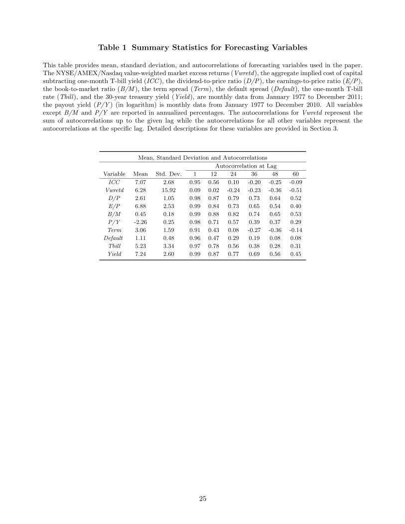
Table 1 Summary Statistics for Forecasting Variables

This table provides mean, standard deviation, and autocorrelations of forecasting variables used in the paper.The NYSE/AMEX/Nasdaq value-weighted market excess returns (Vwretd), the aggregate implied cost of capitalsubtracting one-month T-bill yield (ICC ), the dividend-to-price ratio (D/P), the earnings-to-price ratio (E/P),the book-to-market ratio (B/M ), the term spread (Term), the default spread (Default), the one-month T-billrate (Tbill), and the 30-year treasury yield (Yield), are monthly data from January 1977 to December 2011;the payout yield (P/Y ) (in logarithm) is monthly data from January 1977 to December 2010. All variablesexcept B/M and P/Y are reported in annualized percentages. The autocorrelations for Vwretd represent thesum of autocorrelations up to the given lag while the autocorrelations for all other variables represent theautocorrelations at the specific lag. Detailed descriptions for these variables are provided in Section 3.

Mean, Standard Deviation and Autocorrelations

Autocorrelation at Lag

Variable Mean Std. Dev. 1 12 24 36 48 60

ICC 7.07 2.68 0.95 0.56 0.10 -0.20 -0.25 -0.09

Vwretd 6.28 15.92 0.09 0.02 -0.24 -0.23 -0.36 -0.51

D/P 2.61 1.05 0.98 0.87 0.79 0.73 0.64 0.52

E/P 6.88 2.53 0.99 0.84 0.73 0.65 0.54 0.40

B/M 0.45 0.18 0.99 0.88 0.82 0.74 0.65 0.53

P/Y -2.26 0.25 0.98 0.71 0.57 0.39 0.37 0.29

Term 3.06 1.59 0.91 0.43 0.08 -0.27 -0.36 -0.14

Default 1.11 0.48 0.96 0.47 0.29 0.19 0.08 0.08

Tbill 5.23 3.34 0.97 0.78 0.56 0.38 0.28 0.31

Yield 7.24 2.60 0.99 0.87 0.77 0.69 0.56 0.45

25

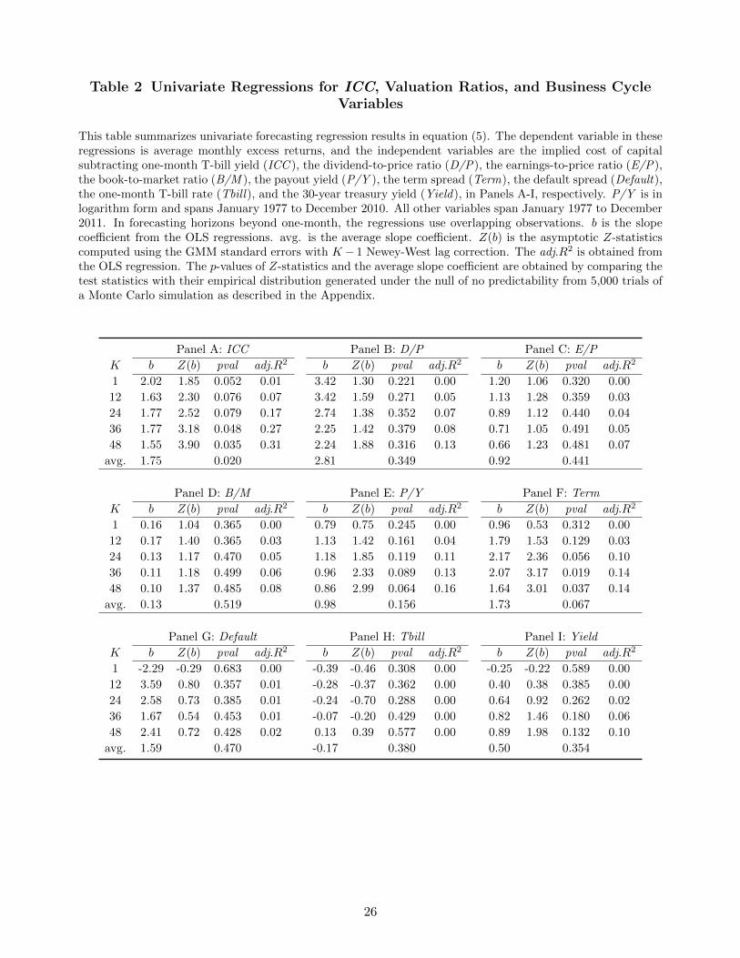
Table 2 Univariate Regressions for ICC, Valuation Ratios, and Business CycleVariables

This table summarizes univariate forecasting regression results in equation (5). The dependent variable in theseregressions is average monthly excess returns, and the independent variables are the implied cost of capitalsubtracting one-month T-bill yield (ICC ), the dividend-to-price ratio (D/P), the earnings-to-price ratio (E/P),the book-to-market ratio (B/M ), the payout yield (P/Y ), the term spread (Term), the default spread (Default),the one-month T-bill rate (Tbill), and the 30-year treasury yield (Yield), in Panels A-I, respectively. P/Y is inlogarithm form and spans January 1977 to December 2010. All other variables span January 1977 to December2011. In forecasting horizons beyond one-month, the regressions use overlapping observations. b is the slopecoefficient from the OLS regressions. avg. is the average slope coefficient. Z(b) is the asymptotic Z-statisticscomputed using the GMM standard errors with K − 1 Newey-West lag correction. The adj.R2 is obtained fromthe OLS regression. The p-values of Z-statistics and the average slope coefficient are obtained by comparing thetest statistics with their empirical distribution generated under the null of no predictability from 5,000 trials ofa Monte Carlo simulation as described in the Appendix.

Panel A: ICC Panel B: D/P Panel C: E/P

K b Z(b) pval adj.R2 b Z(b) pval adj.R2 b Z(b) pval adj.R2

1 2.02 1.85 0.052 0.01 3.42 1.30 0.221 0.00 1.20 1.06 0.320 0.00

12 1.63 2.30 0.076 0.07 3.42 1.59 0.271 0.05 1.13 1.28 0.359 0.03

24 1.77 2.52 0.079 0.17 2.74 1.38 0.352 0.07 0.89 1.12 0.440 0.04

36 1.77 3.18 0.048 0.27 2.25 1.42 0.379 0.08 0.71 1.05 0.491 0.05

48 1.55 3.90 0.035 0.31 2.24 1.88 0.316 0.13 0.66 1.23 0.481 0.07

avg. 1.75 0.020 2.81 0.349 0.92 0.441

Panel D: B/M Panel E: P/Y Panel F: Term

K b Z(b) pval adj.R2 b Z(b) pval adj.R2 b Z(b) pval adj.R2

1 0.16 1.04 0.365 0.00 0.79 0.75 0.245 0.00 0.96 0.53 0.312 0.00

12 0.17 1.40 0.365 0.03 1.13 1.42 0.161 0.04 1.79 1.53 0.129 0.03

24 0.13 1.17 0.470 0.05 1.18 1.85 0.119 0.11 2.17 2.36 0.056 0.10

36 0.11 1.18 0.499 0.06 0.96 2.33 0.089 0.13 2.07 3.17 0.019 0.14

48 0.10 1.37 0.485 0.08 0.86 2.99 0.064 0.16 1.64 3.01 0.037 0.14

avg. 0.13 0.519 0.98 0.156 1.73 0.067

Panel G: Default Panel H: Tbill Panel I: Yield

K b Z(b) pval adj.R2 b Z(b) pval adj.R2 b Z(b) pval adj.R2

1 -2.29 -0.29 0.683 0.00 -0.39 -0.46 0.308 0.00 -0.25 -0.22 0.589 0.00

12 3.59 0.80 0.357 0.01 -0.28 -0.37 0.362 0.00 0.40 0.38 0.385 0.00

24 2.58 0.73 0.385 0.01 -0.24 -0.70 0.288 0.00 0.64 0.92 0.262 0.02

36 1.67 0.54 0.453 0.01 -0.07 -0.20 0.429 0.00 0.82 1.46 0.180 0.06

48 2.41 0.72 0.428 0.02 0.13 0.39 0.577 0.00 0.89 1.98 0.132 0.10

avg. 1.59 0.470 -0.17 0.380 0.50 0.354

26

Table 3 Bivariate Regressions Involving ICC, Valuation Ratios, and BusinessCycle Variables

This table summarizes bivariate forecasting regression results involving ICC and a control variable in equation(5). The control variables are dividend-to-price ratio (D/P), earnings-to-price ratio (E/P), book-to-marketratio (B/M ), the payout yield (P/Y ), the term spread (Term), the default spread (Default), the one-monthT-bill rate (Tbill), and the 30-year treasury yield (Yield), in Panels A-H, respectively. The dependent variablein these regressions is average monthly excess returns. P/Y is in logarithm form and spans January 1977 toDecember 2010. All other variables span January 1977 to December 2011. In forecasting horizons beyond one-month, the regressions use overlapping observations. b and c are the slope coefficients from the OLS regressions.avg. is the average slope coefficient. Z(b) and Z(c) are the asymptotic Z-statistics computed using the GMMstandard errors with K − 1 Newey-West lag correction. The adj.R2 is obtained from the OLS regression. Thep-values of Z-statistics and the average slope coefficient are obtained by comparing the test statistics with theirempirical distribution generated under the null of no predictability from 5,000 trials of a Monte Carlo simulationas described in the Appendix.

Panel A: Bivariate Regression Involving ICC and D/P

ICC D/PK b Z(b) pval c Z(c) pval adj.R2

1 1.79 1.58 0.100 2.24 0.82 0.325 0.0112 1.35 1.88 0.135 2.45 1.18 0.304 0.0824 1.57 2.83 0.058 1.52 1.08 0.357 0.1936 1.62 3.50 0.041 1.01 1.02 0.393 0.2848 1.36 4.00 0.032 1.16 1.51 0.312 0.33

avg. 1.54 0.045 1.68 0.416

Panel B: Bivariate Regression Involving ICC and E/P

ICC E/PK b Z(b) pval c Z(c) pval adj.R2

1 1.87 1.70 0.085 0.79 0.70 0.381 0.0112 1.46 2.08 0.112 0.81 1.01 0.369 0.0824 1.66 2.75 0.071 0.50 0.95 0.400 0.1836 1.69 3.50 0.044 0.35 0.89 0.433 0.2748 1.46 4.17 0.034 0.36 1.17 0.391 0.32

avg. 1.63 0.043 0.56 0.478

Panel C: Bivariate Regression Involving ICC and B/M

ICC B/MK b Z(b) pval c Z(c) pval adj.R2

1 1.87 1.66 0.089 0.08 0.51 0.510 0.0112 1.41 1.98 0.126 0.11 0.94 0.424 0.0724 1.64 2.87 0.060 0.06 0.76 0.489 0.1836 1.67 3.58 0.038 0.04 0.65 0.532 0.2748 1.44 3.91 0.035 0.04 0.79 0.517 0.31

avg. 1.61 0.048 0.07 0.563

Panel D: Bivariate Regression Involving ICC and P/Y

ICC P/YK b Z(b) pval c Z(c) pval adj.R2

1 2.16 1.88 0.053 0.06 0.05 0.513 0.0112 1.22 1.82 0.139 0.68 0.85 0.297 0.0724 1.26 2.08 0.130 0.73 1.23 0.238 0.1736 1.59 3.16 0.057 0.41 1.29 0.243 0.2948 1.28 3.45 0.056 0.41 1.77 0.186 0.32

avg. 1.50 0.051 0.46 0.344

27

Panel E: Bivariate Regression Involving ICC and Term

ICC TermK b Z(b) pval c Z(c) pval adj.R2

1 4.44 2.51 0.009 -5.06 -1.78 0.951 0.0112 2.15 1.66 0.158 -1.10 -0.53 0.632 0.0724 1.96 1.60 0.197 -0.40 -0.25 0.543 0.1736 1.93 2.05 0.141 -0.31 -0.27 0.544 0.2648 1.85 3.47 0.039 -0.62 -1.06 0.744 0.31

avg. 2.47 0.019 -1.50 0.801

Panel F: Bivariate Regression Involving ICC and Default

ICC DefaultK b Z(b) pval c Z(c) pval adj.R2

1 2.54 2.37 0.013 -7.62 -0.97 0.837 0.0112 1.62 2.18 0.086 0.13 0.03 0.494 0.0624 1.88 2.81 0.053 -1.45 -0.54 0.643 0.1736 1.92 3.42 0.038 -2.06 -0.83 0.707 0.2748 1.58 3.58 0.040 -0.64 -0.23 0.563 0.30

avg. 1.91 0.010 -2.33 0.698

Panel G: Bivariate Regression Involving ICC and Tbill

ICC TbillK b Z(b) pval c Z(c) pval adj.R2

1 2.14 1.90 0.043 0.24 0.28 0.646 0.0012 1.71 2.19 0.076 0.20 0.27 0.623 0.0624 1.84 2.32 0.085 0.20 0.56 0.699 0.1736 1.83 3.08 0.044 0.23 0.87 0.758 0.2748 1.62 4.00 0.020 0.35 1.50 0.856 0.32

avg. 1.83 0.010 0.24 0.698

Panel H: Bivariate Regression Involving ICC and Yield

ICC YieldK b Z(b) pval c Z(c) pval adj.R2

1 2.02 1.85 0.052 -0.23 -0.21 0.482 0.0012 1.62 2.25 0.082 0.34 0.37 0.312 0.0624 1.73 2.56 0.078 0.47 0.91 0.201 0.1836 1.67 3.22 0.056 0.49 1.36 0.145 0.2848 1.41 3.80 0.039 0.53 1.75 0.118 0.34

avg. 1.69 0.021 0.32 0.302

28

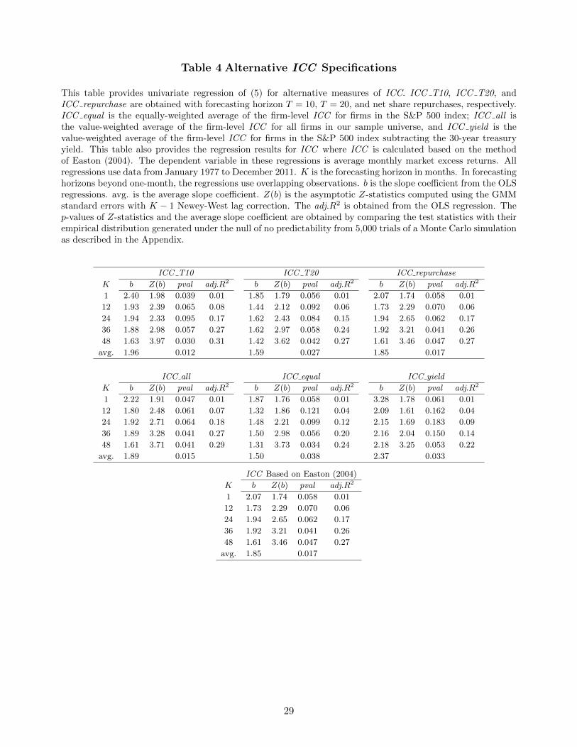
Table 4 Alternative ICC Specifications

This table provides univariate regression of (5) for alternative measures of ICC. ICC T10, ICC T20, andICC repurchase are obtained with forecasting horizon T = 10, T = 20, and net share repurchases, respectively.ICC equal is the equally-weighted average of the firm-level ICC for firms in the S&P 500 index; ICC all isthe value-weighted average of the firm-level ICC for all firms in our sample universe, and ICC yield is thevalue-weighted average of the firm-level ICC for firms in the S&P 500 index subtracting the 30-year treasuryyield. This table also provides the regression results for ICC where ICC is calculated based on the methodof Easton (2004). The dependent variable in these regressions is average monthly market excess returns. Allregressions use data from January 1977 to December 2011. K is the forecasting horizon in months. In forecastinghorizons beyond one-month, the regressions use overlapping observations. b is the slope coefficient from the OLSregressions. avg. is the average slope coefficient. Z(b) is the asymptotic Z-statistics computed using the GMMstandard errors with K − 1 Newey-West lag correction. The adj.R2 is obtained from the OLS regression. Thep-values of Z-statistics and the average slope coefficient are obtained by comparing the test statistics with theirempirical distribution generated under the null of no predictability from 5,000 trials of a Monte Carlo simulationas described in the Appendix.

ICC T10 ICC T20 ICC repurchase

K b Z(b) pval adj.R2 b Z(b) pval adj.R2 b Z(b) pval adj.R2

1 2.40 1.98 0.039 0.01 1.85 1.79 0.056 0.01 2.07 1.74 0.058 0.01

12 1.93 2.39 0.065 0.08 1.44 2.12 0.092 0.06 1.73 2.29 0.070 0.06

24 1.94 2.33 0.095 0.17 1.62 2.43 0.084 0.15 1.94 2.65 0.062 0.17

36 1.88 2.98 0.057 0.27 1.62 2.97 0.058 0.24 1.92 3.21 0.041 0.26

48 1.63 3.97 0.030 0.31 1.42 3.62 0.042 0.27 1.61 3.46 0.047 0.27

avg. 1.96 0.012 1.59 0.027 1.85 0.017

ICC all ICC equal ICC yield

K b Z(b) pval adj.R2 b Z(b) pval adj.R2 b Z(b) pval adj.R2

1 2.22 1.91 0.047 0.01 1.87 1.76 0.058 0.01 3.28 1.78 0.061 0.01

12 1.80 2.48 0.061 0.07 1.32 1.86 0.121 0.04 2.09 1.61 0.162 0.04

24 1.92 2.71 0.064 0.18 1.48 2.21 0.099 0.12 2.15 1.69 0.183 0.09

36 1.89 3.28 0.041 0.27 1.50 2.98 0.056 0.20 2.16 2.04 0.150 0.14

48 1.61 3.71 0.041 0.29 1.31 3.73 0.034 0.24 2.18 3.25 0.053 0.22

avg. 1.89 0.015 1.50 0.038 2.37 0.033

ICC Based on Easton (2004)

K b Z(b) pval adj.R2

1 2.07 1.74 0.058 0.01

12 1.73 2.29 0.070 0.06

24 1.94 2.65 0.062 0.17

36 1.92 3.21 0.041 0.26

48 1.61 3.46 0.047 0.27

avg. 1.85 0.017

29

Table 5 Univariate Regressions for Size and B/M Portfolios.

This table summarizes univariate forecasting regression results for size and B/M portfolios. Small Size, MediumSize, and Large Size are the three size portfolios, and Low B/M, Median B/M, and High B/M are the threebook-to-market portfolios. The dependent variable in these regressions is average monthly excess returns for thecorresponding portfolio, and the independent variables are the implied cost of capital (ICC ), the dividend-to-price ratio (D/P), the earnings-to-price ratio (E/P), and the book-to-market ratio (B/M ) for the correspondingportfolio. All variables span January 1977 to December 2011. In forecasting horizons beyond one-month, theregressions use overlapping observations. b is the slope coefficient from the OLS regressions. avg. is the averageslope coefficient. Z(b) is the asymptotic Z-statistics computed using the GMM standard errors with K − 1Newey-West lag correction. The adj.R2 is obtained from the OLS regression. The p-values of Z-statisticsand the average slope coefficient are obtained by comparing the test statistics with their empirical distributiongenerated under the null of no predictability from 5,000 trials of a Monte Carlo simulation as described in theAppendix.

Panel A: Univariate Regressions for Small Size PortfolioICC D/P E/P B/M

K b Z(b) pval adj.R2 b Z(b) pval adj.R2 b Z(b) pval adj.R2 b Z(b) pval adj.R2

1 4.11 2.70 0.005 0.02 4.75 0.99 0.248 0.00 2.38 1.76 0.073 0.01 0.33 1.68 0.091 0.0112 2.68 3.21 0.017 0.11 6.49 1.94 0.129 0.06 2.62 2.87 0.053 0.12 0.44 3.53 0.016 0.1624 1.71 1.99 0.127 0.12 4.09 2.18 0.120 0.07 1.60 2.34 0.114 0.13 0.27 2.85 0.072 0.1836 1.28 1.68 0.195 0.12 3.01 1.94 0.190 0.07 1.30 2.57 0.126 0.15 0.21 2.75 0.103 0.1948 0.61 1.06 0.344 0.04 2.36 1.63 0.270 0.07 1.13 2.61 0.153 0.18 0.18 2.72 0.135 0.22

avg. 2.08 0.014 4.14 0.244 1.81 0.121 0.29 0.064

Panel B: Univariate Regressions for Medium Size PortfolioICC D/P E/P B/M

K b Z(b) pval adj.R2 b Z(b) pval adj.R2 b Z(b) pval adj.R2 b Z(b) pval adj.R2

1 3.80 2.64 0.009 0.02 2.17 0.58 0.416 0.00 1.95 1.44 0.167 0.01 0.33 1.59 0.122 0.0112 2.50 3.44 0.015 0.11 4.14 1.65 0.190 0.04 1.71 2.08 0.165 0.06 0.36 3.03 0.041 0.1124 1.92 3.01 0.041 0.21 2.40 1.35 0.305 0.05 0.95 1.65 0.284 0.06 0.21 2.27 0.152 0.1136 1.43 3.01 0.063 0.23 1.90 1.45 0.334 0.06 0.73 1.86 0.273 0.07 0.15 2.42 0.166 0.1348 0.82 2.73 0.094 0.13 1.55 1.73 0.315 0.07 0.59 1.96 0.291 0.08 0.11 2.39 0.189 0.12

avg. 2.10 0.015 2.43 0.402 1.19 0.345 0.23 0.194

Panel C: Univariate Regressions for Large Size PortfolioICC D/P E/P B/M

K b Z(b) pval adj.R2 b Z(b) pval adj.R2 b Z(b) pval adj.R2 b Z(b) pval adj.R2

1 1.77 1.67 0.073 0.01 2.87 1.13 0.280 0.00 0.94 0.85 0.352 0.00 0.13 0.83 0.403 0.0012 1.42 2.07 0.089 0.05 2.74 1.35 0.326 0.03 0.84 0.98 0.408 0.02 0.13 1.10 0.422 0.0224 1.59 2.37 0.095 0.14 2.21 1.15 0.423 0.05 0.64 0.83 0.485 0.02 0.10 0.87 0.515 0.0336 1.70 3.08 0.060 0.22 1.89 1.16 0.472 0.06 0.52 0.75 0.525 0.03 0.09 0.84 0.548 0.0348 1.54 3.85 0.035 0.25 1.95 1.47 0.444 0.09 0.51 0.85 0.539 0.04 0.08 0.93 0.559 0.05

avg. 1.60 0.025 2.33 0.418 0.69 0.424 0.11 0.497

Panel D: Univariate Regressions for Low B/M PortfolioICC D/P E/P B/M

K b Z(b) pval adj.R2 b Z(b) pval adj.R2 b Z(b) pval adj.R2 b Z(b) pval adj.R2

1 2.51 1.99 0.041 0.01 2.97 0.76 0.358 0.00 1.47 0.93 0.328 0.00 0.15 0.61 0.460 0.0012 1.71 1.96 0.115 0.05 3.05 1.02 0.354 0.02 1.36 1.13 0.367 0.02 0.17 0.84 0.453 0.0124 1.66 2.03 0.123 0.11 1.77 0.62 0.480 0.02 0.90 0.79 0.473 0.02 0.09 0.48 0.589 0.0136 1.77 2.57 0.083 0.17 1.20 0.49 0.537 0.01 0.65 0.64 0.556 0.02 0.08 0.46 0.617 0.0148 1.59 2.62 0.092 0.18 1.16 0.51 0.547 0.02 0.56 0.62 0.592 0.02 0.06 0.41 0.634 0.01

avg. 1.85 0.029 2.03 0.452 0.99 0.460 0.11 0.579

30

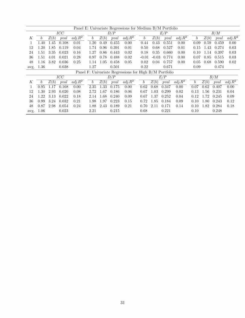
Panel E: Univariate Regressions for Medium B/M PortfolioICC D/P E/P B/M

K b Z(b) pval adj.R2 b Z(b) pval adj.R2 b Z(b) pval adj.R2 b Z(b) pval adj.R2

1 1.40 1.45 0.108 0.01 1.20 0.49 0.455 0.00 0.44 0.43 0.551 0.00 0.09 0.59 0.459 0.0012 1.20 1.85 0.119 0.04 1.74 0.96 0.391 0.01 0.50 0.68 0.527 0.01 0.15 1.43 0.274 0.0324 1.51 3.35 0.023 0.16 1.27 0.86 0.443 0.02 0.18 0.35 0.660 0.00 0.10 1.14 0.397 0.0336 1.51 4.01 0.021 0.28 0.97 0.78 0.488 0.02 -0.01 -0.03 0.774 0.00 0.07 0.85 0.515 0.0348 1.16 3.82 0.036 0.25 1.14 1.05 0.458 0.05 0.02 0.04 0.757 0.00 0.05 0.68 0.590 0.02

avg. 1.36 0.038 1.27 0.501 0.22 0.671 0.09 0.474

Panel F: Univariate Regressions for High B/M PortfolioICC D/P E/P B/M

K b Z(b) pval adj.R2 b Z(b) pval adj.R2 b Z(b) pval adj.R2 b Z(b) pval adj.R2

1 0.95 1.17 0.168 0.00 2.35 1.33 0.175 0.00 0.62 0.68 0.347 0.00 0.07 0.62 0.407 0.0012 1.30 2.93 0.020 0.08 2.72 1.67 0.186 0.06 0.67 1.03 0.299 0.02 0.13 1.56 0.231 0.0424 1.22 3.13 0.022 0.18 2.14 1.68 0.240 0.09 0.67 1.37 0.252 0.04 0.12 1.72 0.245 0.0936 0.99 3.24 0.032 0.21 1.98 1.97 0.223 0.15 0.72 1.85 0.184 0.09 0.10 1.80 0.243 0.1248 0.87 2.98 0.054 0.24 1.88 2.43 0.189 0.21 0.70 2.11 0.171 0.14 0.10 1.82 0.284 0.18

avg. 1.06 0.023 2.21 0.215 0.68 0.221 0.10 0.248

31

Table 6 Out-of-Sample Test

This table summarizes the out-of-sample analysis of forecasting models using different forecasting variables forthe forecast period of January 1998 to December 2011. Panel A reports the R2

os statistic of Campbell andThompson (2008). Panel A also reports the utility gain (Ugain), which is the portfolio management fee (inannualized percentage return) that an investor with mean-variance preferences and risk aversion coefficient ofthree would be willing to pay to have access to the forecasting model using a particular forecasting variablerelative to the historical average benchmark forecasting model; the weight on stocks in the investor’s portfolio isconstrained to lie between zero and 1.5 (inclusive). Panel B reports the p-values of the forecasting encompassingtest statistic of Harvey, Leybourne, and Newbold (1998) (HLN statistic), which corresponds to a one-sided(upper-tail) test of the null hypothesis that the forecast from the row variable (R) encompasses the forecastfrom the column variable (C) against the alternative hypothesis that the forecast from the row variable (R)does not encompass the forecast from the column variable (C). The dependent variable in these regressions ismonthly market excess returns. In these tests, we perform a 2-year moving average for ICC.

Panel A: Out-of-Sample R2os and Utility Gains

R2os pval Ugain

IRP 1.22 0.06 4.15D/P 0.44 0.16 1.38E/P 0.22 0.27 0.40B/M 0.26 0.23 0.57Term -0.53 -1.32

Default -0.90 -1.33Tbill -1.18 -2.21Yield -1.62 -1.84

Panel B: Forecast Encompassing TestColumn Variables (C)

Row Variables (R) ICC E/P D/P B/M Term Default Tbill YieldICC 0.40 0.50 0.51 0.76 0.71 0.84 0.79E/P 0.09 0.70 0.70 0.71 0.74 0.73 0.76D/P 0.07 0.23 0.41 0.69 0.69 0.73 0.73B/M 0.07 0.22 0.55 0.73 0.73 0.77 0.77Term 0.03 0.07 0.10 0.09 0.53 0.74 0.66

Default 0.04 0.11 0.16 0.14 0.29 0.44 0.51Tbill 0.01 0.03 0.04 0.03 0.10 0.28 0.67Yield 0.01 0.02 0.04 0.03 0.09 0.18 0.19

32

0.0%

2.0%

6.0%

14.0

%

12.0

%

2.6%

Ja

n 20

00

Sep

200

29.

4%

Jun

2007

4.4%

Mar

200

912

.8%

Dec

201

19.

7%

Percentage per Year

Jan 77

Jan 80

Jan 83

Jan 86

Jan 89

Jan 92

Jan 95

Jan 98

Jan 01

Jan 04

Jan 07

Jan 10

NB

ER

Rec

essi

on P

erio

dsH

isto

rical

Med

ian

Med

ian

± 2

Sig

ma

Mea

n

7.1%

STD

EV

2.7%

Med

ian

7.4%

10.0

%

8.0%

4.0%

Fig

ure

1:

Aggr

egate

Imp

lied

Cost

of

Cap

ital

(IC

C).

Th

isfi

gure

dep

icts

the

valu

e-w

eigh

ted

imp

lied

cost

ofca

pit

al

con

stru

cted

bas

edon

pre

vail

ing

S&

P500

com

pan

ies

from

Jan

uary

1977

toD

ecem

ber

2011

sub

trac

tin

gth

eon

e-m

onth

T-b

ill

yie

ld.

ICC

isex

pre

ssed

inan

nu

ali

zed

per

centa

ges.

Th

eth

ree

hor

izon

tal

dash

edcu

rves

corr

esp

ond

toth

ero

llin

gm

edia

nan

dth

etw

o-s

tan

dar

d-d

evia

tion

ban

ds

calc

ula

ted

usi

ng

all

his

tori

cal

dat

ast

art

ing

from

Jan

uary

1987

.T

he

shad

edar

eas

ind

icat

eth

eN

BE

Rre

cess

ion

per

iod

s.T

he

nu

mb

ers

asso

ciate

dw

ith

the

arr

ows

are

the

ICC

sfo

rre

cent

imp

orta

nt

date

s.T

he

his

tori

cal

mea

n,

med

ian

and

stan

dar

dd

evia

tion

sof

ICC

are

pro

vid

edin

the

box

un

der

the

gra

ph

.

33

Jan98 Jan01 Jan04 Jan07 Jan10−5

0

5

10x 10

−3 ICC

Jan98 Jan01 Jan04 Jan07 Jan10−2

−1

0

1

2

3x 10

−3 D/P

Jan98 Jan01 Jan04 Jan07 Jan10−2

−1

0

1

2

3x 10

−3 E/P

Jan98 Jan01 Jan04 Jan07 Jan10−2

−1

0

1

2

3x 10

−3 B/M

Jan98 Jan01 Jan04 Jan07 Jan10−3

−2

−1

0

1

2x 10

−3 Term

Jan98 Jan01 Jan04 Jan07 Jan10−4

−2

0

2

4x 10

−3 Default

Jan98 Jan01 Jan04 Jan07 Jan10−6

−4

−2

0

2x 10

−3 Tbill

Jan98 Jan01 Jan04 Jan07 Jan10−8

−6

−4

−2

0

2x 10

−3 Yield

Figure 2: Cumulative squared prediction error for the historical average benchmark forecasting modelminus the cumulative squared prediction error for the forecasting model using the implied cost ofcapital (ICC ), dividend-to-price ratio (D/P), earnings-to-price ratio (E/P), book-to-market ratio(B/M ), term spread (Term), default spread (Default), T-bill rate (Tbill), and 30-year treasury yield(Yield), during the forecast period of January 1998 to December 2011. The dotted line in each panelgoes through zero.

34