Embed Size (px)
Citation preview
1. Report No. FHWA/TX-09/0-5627-1
2. Government Accession No.
3. Recipient's Catalog No.
4. Title and Subtitle PREDICTING ASPHALT MIXTURE SKID RESISTANCE BASED ON AGGREGATE CHARACTERISTICS
5. Report Date October 2008 Published: August 2009 6. Performing Organization Code
7. Author(s) Eyad Masad, Arash Rezaei, Arif Chowdhury, and Pat Harris
8. Performing Organization Report No. Report 0-5627-1
9. Performing Organization Name and Address Texas Transportation Institute The Texas A&M University System College Station, Texas 77843-3135
10. Work Unit No. (TRAIS) 11. Contract or Grant No. Project 0-5627
12. Sponsoring Agency Name and Address Texas Department of Transportation Research and Technology Implementation Office P.O. Box 5080 Austin, Texas 78763-5080
13. Type of Report and Period Covered Technical Report: September 2006 – August 2008 14. Sponsoring Agency Code
15. Supplementary Notes Project performed in cooperation with the Texas Department of Transportation and the Federal Highway Administration. Project Title: Aggregate Resistance to Polishing and Its Relationship to Skid Resistance URL: http://tti.tamu.edu/documents/ 0-5627-1.pdf 16. Abstract The objective of this research project was to develop a method to determine the skid resistance of an asphalt mixture based on aggregate characteristics and gradation. Asphalt mixture slabs with different combinations of aggregate sources and mixture designs were fabricated in the laboratory, and their skid resistance was measured after different polishing intervals. The wheel-polishing device developed by the National Center for Asphalt Technology (NCAT) was used for polishing the slabs. Frictional characteristics of each slab were measured by sand patch method, British Pendulum, Dynamic Friction Tester (DFT), and Circular Texture Meter (CTMeter). Aggregates were characterized using a number of conventional test methods, and aggregate texture was measured using the Aggregate Imaging System (AIMS) after different polishing intervals in the Micro-Deval device. Petrographic analyses were performed using thin sections made with aggregates from each of these sources. Petrographic analyses provided the mineralogical composition of each source. The aggregate gradation was quantified by fitting the cumulative Weibull distribution function to the gradation curve. This function allows describing the gradation by using only two parameters.
The results of the analysis confirmed a strong relationship between mix frictional properties and aggregate properties. The main aggregate properties affecting the mix skid resistance were Polish Stone Value, texture change before and after Micro-Deval measured by AIMS, terminal texture after Micro-Deval measured by AIMS, and coarse aggregate acid insolubility value.
The analysis has led to the development of a model for the International Friction Index (IFI) of asphalt mixtures as a function of polishing cycles. The parameters of this model were determined as functions of (a) initial and terminal aggregate texture measured using AIMS, (b) rate of change in aggregate texture measured using AIMS after different polishing intervals, and the (c) Weibull distribution parameters describing aggregate gradation. This model allows estimating the frictional characteristics of an asphalt mixture during the mixture design stage. 17. Key Words Skid Resistance, Asphalt Mixture Polishing, Aggregate Characteristics
18. Distribution Statement No restrictions. This document is available to the public through NTIS: National Technical Information Service Springfield, Virginia 22161 http://www.ntis.gov No restrictions
19. Security Classif.(of this report) Unclassified
20. Security Classif.(of this page) Unclassified
21. No. of Pages 226
22. Price


PREDICTING ASPHALT MIXTURE SKID RESISTANCE BASED ON AGGREGATE CHARACTERISTICS
by
Eyad Masad, Ph.D., P.E. E.B. Snead I Associate Professor
Zachry Department of Civil Engineering Texas A&M University
Arash Rezaei
Graduate Research Assistant Zachry Department of Civil Engineering
Texas A&M University
Arif Chowdhury Assistant Research Engineer
Texas Transportation Institute
and
Pat Harris Associate Research Scientist
Texas Transportation Institute
Report 0-5627-1 Project 0-5627
Project Title: Aggregate Resistance to Polishing and Its Relationship to Skid Resistance
Performed in cooperation with the Texas Department of Transportation
and the Federal Highway Administration
October 2008 Published: August 2009
TEXAS TRANSPORTATION INSTITUTE The Texas A&M University System College Station, Texas 77843-3135


v
DISCLAIMER
The contents of this report reflect the views of the authors, who are responsible
for the facts and accuracy of the data presented herein. The contents do not necessarily
reflect the official view or policies of the Federal Highway Administration (FHWA) or
the Texas Department of Transportation (TxDOT). This report does not constitute a
standard, specification, or regulation. The engineer in charge was Eyad Masad P.E.
#96368.

vi
ACKNOWLEDGMENTS
The authors wish to express their appreciation to the Texas Department of
Transportation personnel for their support throughout this project, as well as the Federal
Highway Administration. The authors would also like to thank the project director,
Ms. Caroline Herrera, and the members of the project monitoring committee,
Mr. Ed Morgan and Ms. Zyna Polanski, for their constant guidance and valuable
technical comments during this project.
vii
TABLE OF CONTENTS
LIST OF FIGURES ........................................................................................................... ix
LIST OF TABLES ........................................................................................................... xiv
CHAPTER I − INTRODUCTION ..................................................................................... 1
Problem Statement .......................................................................................................... 3 Objectives ....................................................................................................................... 3 Scope of the Study .......................................................................................................... 4 Organization of the Report ............................................................................................. 4
CHAPTER II − LITERATURE REVIEW ......................................................................... 5
Introduction ..................................................................................................................... 5 Definition of Friction ...................................................................................................... 5 Pavement Texture ........................................................................................................... 7 Texture and Friction Measurement ............................................................................... 12 Skid Resistance Variation ............................................................................................. 22
Age of the Surface .................................................................................................... 22 Seasonal and Daily Variation.................................................................................... 23
Aggregate Polishing Characteristics ............................................................................. 25 Pre - Evaluating of Aggregate for Use in Asphalt Mixture .......................................... 28 Predictive Models for Skid Resistance ......................................................................... 32 International Friction Index .......................................................................................... 34 Wet Weather Accident Reduction Program (WWARP) ............................................... 37
CHAPTER III − MATERIALS AND EXPERIMENTAL DESIGN ............................... 41
Introduction ................................................................................................................... 41 Aggregate Sources ........................................................................................................ 41 Petrographic Analysis of Aggregates with Respect to Skid Resistance ....................... 44
Beckman Pit .............................................................................................................. 45 Brownlee Pit.............................................................................................................. 47 Brownwood Pit ......................................................................................................... 50 Fordyce Pit ................................................................................................................ 53 McKelligon Pit .......................................................................................................... 54 Georgetown Pit ......................................................................................................... 58
Testing of Aggregate Resistance to Polishing and Degradation ................................... 60 Los Angeles Abrasion and Impact Test .................................................................... 61 Magnesium Sulfate Soundness ................................................................................. 61 British Pendulum Test ............................................................................................... 62 Micro -Deval Test ..................................................................................................... 62 Aggregate Imaging System ....................................................................................... 64
Asphalt Mixture Types ................................................................................................. 65 Type C Mix Design ................................................................................................... 65 Type D Mix Design .................................................................................................. 66 Porous Friction Course ............................................................................................. 66
viii
Asphalt Mixture Preparation ......................................................................................... 67 Slab-Polishing Methods ................................................................................................ 72 Testing of Mixture Resistance to Polishing .................................................................. 75
British Pendulum Skid Tester ................................................................................... 75 The Volumetric Method for Measuring Macrotexture – Sand Patch Method .......... 77 Dynamic Friction Tester ........................................................................................... 77 Circular Texture Meter ............................................................................................. 79
Experimental Setup ....................................................................................................... 79
CHAPTER IV − RESULTS AND DATA ANALYSIS ................................................... 83
Introduction ................................................................................................................... 83 Aggregate Characteristics ............................................................................................. 83 Mixture-Polishing Characteristics ................................................................................ 88
Results of the Sand Patch Test .................................................................................. 89 Results of the British Pendulum Test ........................................................................ 94 Results of CTMeter and DFT ................................................................................. 106
Aggregate Ranking Based on Lab Results ................................................................. 126
CHAPTER V – MIX FRICTION MODEL BASED ON AGGREGATE PROPERTIES ................................................................................................................. 129
Introduction ................................................................................................................. 129 Modeling Approach .................................................................................................... 129
CHAPTER VI − RESULTS AND CONCLUSIONS ..................................................... 143
Introduction ................................................................................................................. 143 Sand Patch Test ........................................................................................................... 143 British Pendulum Test ................................................................................................ 143 CTMeter and DFT Tests ............................................................................................. 144 Summary ..................................................................................................................... 146
REFERENCES ............................................................................................................... 149
APPENDIX A− MIXTURE DESIGNS ......................................................................... 167
APPENDIX B – TEXTURE AND ANGULARITY MEASUREMENTS BY AIMS FOR DIFFERENT AGGREGATES............................................................................... 181
APPENDIX C – PLOTS OF TERMINAL AND RATE OF CHANGE VALUES FOR F60 AND DF20 FOR DIFFERENT AGGREGATE AND MIXES ....................... 187
ix
LIST OF FIGURES
Figure 1. Schematic Plot of Hysteresis and Adhesion (Choubane et al., 2004). ................ 7 Figure 2. Pavement Wavelength and Surface Characteristics (Hall et al., 2006). .............. 9 Figure 3. Schematic Plot of Microtexture/Macrotexture (Noyce et al., 2005). ................ 10 Figure 4. Schematic Plot of the Effect of Microtexture/Macrotexture on Pavement
Friction (Noyce et al., 2005). ........................................................................ 12 Figure 5. Different Data Acquisition Methods (Johnsen, 1997). ...................................... 18 Figure 6. Decrease of Pavement Skid Resistance due to Polishing of Traffic
(Skeritt, 1993). ............................................................................................... 23 Figure 7. Generalized Pavement-Polishing Model (after Chelliah et al., 2003). .............. 24 Figure 8. Aggregate Methods for Providing Pavement Texture (Dahir, 1979). ............... 28 Figure 9. Mineral Composition Related to Skid Resistance (Mullen et al., 1974). .......... 33 Figure 10. First Aggregate Classification Chart. .............................................................. 38 Figure 11. Modified Aggregate Classification Chart (Second Edition). .......................... 39 Figure 12. Map of Texas Showing Aggregate Quarries by County Location. ................. 42 Figure 13. Aggregate Classification Based on Old Aggregate Classification System. .... 43 Figure 14. Micritic, Low Porosity Limestone from the Beckman Pit. ............................. 46 Figure 15. Grainstone with Coated Fossil Fragments from the Beckman Pit. ................. 46 Figure 16. Coarsely Crystalline Limestone with Moldic Pores from the Beckman Pit. ... 47 Figure 17. Glauconitic Dolomite from the Brownlee Pit. ................................................. 48 Figure 18. Calcite and Dolomite-Cemented Sandstone from the Brownlee Pit. .............. 49 Figure 19. Heavily Weathered Dolomite from the Brownlee Pit. .................................... 50 Figure 20. Sandy Dolomitic Limestone from the Brownwood Pit. .................................. 51 Figure 21. Calcite and Dolomite-Cemented Sandstone from the Brownwood Pit. .......... 52 Figure 22. Carbonate-Cemented Sandstone with Abundant Heavy Minerals. ................. 52 Figure 23. Chalcedony Replacement of Fossils and Moldic Porosity of Fordyce Pit. ..... 53 Figure 24. Chalcedony Matrix with Moldic Pores from the Fordyce Pit. ........................ 54 Figure 25. Sandy Dolomite from the El Paso, McKelligon Pit. ....................................... 55 Figure 26. Fine-Grained Limestone from the El Paso, McKelligon Pit. .......................... 56 Figure 27. Dolomite and Siderite-Cemented Sandstone from the McKelligon Pit. ......... 57 Figure 28. Cross-Polarized Light View of Altered Granite from McKelligon Pit. .......... 58 Figure 29. Fine-Grained Limestone with Chalcedony from the Georgetown Pit. ............ 59 Figure 30. Moldic Pores in Limestone from the Georgetown Pit. .................................... 59 Figure 31. Micro-Deval Apparatus. .................................................................................. 63 Figure 32. Mechanism of Aggregate and Steel Balls Interaction in Micro-Deval
Apparatus. ...................................................................................................... 63 Figure 33. Schematic View of the AIMS System. ............................................................ 65 Figure 34. Schematic Layout of Each Slab. ...................................................................... 68 Figure 35. Schematic of the Mold Used in Slab Compaction. .......................................... 70 Figure 36. Slab Thickness Measuring Scale Used to Adjust Slab Thickness. .................. 70 Figure 37. Walk-Behind Roller Compactor. ..................................................................... 71 Figure 38. Schematic View of MMLS3 (after Hugo 2005). ............................................. 73 Figure 39. Polishing Machine Assembly. ......................................................................... 75 Figure 40. British Pendulum Device. ................................................................................ 76
x
Figure 41. Schematic of Sand Patch Method. ................................................................... 77 Figure 42. Schematic of Measuring Pavement Skid Resistance by DFT. ........................ 78 Figure 43. CTMeter (Courtesy of Hanson and Prowell, 2004)......................................... 79 Figure 44. Type D Mixes Degraded after 5000 Cycles. ................................................... 81 Figure 45. Floor Polisher. ................................................................................................. 82 Figure 46. Aggregate Properties (after Alvarado et al., 2006; TxDOT BRSQ, 2008). .... 84 Figure 47. Aggregate Texture before and after Micro-Deval and Percent Change. ......... 86 Figure 48. Aggregate Angularity before and after Micro-Deval and Percent Change. .... 86 Figure 49. Aggregate Texture as Function of Micro-Deval Time (Masad et al., 2005). .. 88 Figure 50. Measured MTD by Sand Patch Method for Different Aggregates .................. 89 Figure 51. Results of British Pendulum Test for Type C Mixes. ..................................... 94 Figure 52. Results of the British Pendulum Test for PFC Mixes. .................................... 94 Figure 53. British Pendulum Values for El Paso Aggregate vs. Polishing Cycles. .......... 99 Figure 54. British Pendulum Values for Beckman Aggregate vs. Polishing Cycles. ....... 99 Figure 55. British Pendulum Values for Brownwood Aggregate vs. Polishing Cycles. 100 Figure 56. British Pendulum Values for Brownlee Aggregate vs. Polishing Cycles. .... 100 Figure 57. British Pendulum Values for Fordyce Aggregate vs. Polishing Cycles. ....... 101 Figure 58. British Pendulum Values for the 50 Percent Beckman 50 Percent ............... 101 Figure 59. British Pendulum Values for El Paso Aggregate vs. Polishing Cycles in
PFC Mix. ..................................................................................................... 102 Figure 60. British Pendulum Values for Brownlee Aggregate vs. Polishing ................. 102 Figure 61. British Pendulum Values for Brownwood Aggregate vs. Polishing ............. 103 Figure 62. British Pendulum Values for Beckman Aggregate vs. Polishing .................. 103 Figure 63. Calculated F60 for Different Aggregate vs. Polishing Cycle. ....................... 106 Figure 64. Coefficient of Friction for Different Aggregate vs. Polishing
Cycle at 20 km/h. ......................................................................................... 107 Figure 65. MPD for Different Aggregate vs. Polishing Cycle. ...................................... 107 Figure 66. Calculated F60 Values vs. Polishing Cycle and Fitted Line
for PFC Mixes. ............................................................................................ 115 Figure 67. Calculated F60 Values vs. Polishing Cycle and Fitted Line
for Type C Mixes. ....................................................................................... 115 Figure 68. DF20 Values vs. Polishing Cycle and Fitted Line for Type C Mixes. ........... 116 Figure 69. DF20 Values vs. Polishing Cycle and Fitted Line for PFC Mixes. ................ 116 Figure 70. Terminal F60 Values for Different Aggregate Types. .................................. 118 Figure 71. Rate of F60 Change for Different Aggregate Types. .................................... 119 Figure 72. Initial F60 Values for Different Aggregate Types. ....................................... 119 Figure 73. Terminal DF20 Values for Different Aggregate Types. ................................. 120 Figure 74. Rate of DF20 Change for Different Aggregate Types. ................................... 120 Figure 75. Initial DF20 Values for Different Aggregate Types. ...................................... 121 Figure 76. Mean F60 Values for Different Aggregate Types. ........................................ 127 Figure 77. Overview of the Friction Model. ................................................................... 129 Figure 78. Aggregate Gradation and Fitted Line for Brownlee-Beckman
Type C Mix. ................................................................................................ 130 Figure 79. Aggregate Gradation and Fitted Line for Fordyce Aggregate
Type C Mix. ................................................................................................ 131
xi
Figure 80. Aggregate Gradation and Fitted Line for Brownwood Aggregate Type C Mix. ................................................................................................ 131
Figure 81. Aggregate Gradation and Fitted Line for Brownlee Aggregate Type C Mix. ................................................................................................ 132
Figure 82. Aggregate Gradation and Fitted Line for Beckman Aggregate Type C Mix. ................................................................................................ 132
Figure 83. Aggregate Gradation and Fitted Line for El Paso Aggregate Type C Mix. ................................................................................................ 133
Figure 84. Aggregate Gradation and Fitted Line for Brownwood Aggregate PFC Mix. ..................................................................................................... 133
Figure 85. Aggregate Gradation and Fitted Line for Beckman Aggregate PFC Mix. ..................................................................................................... 134
Figure 86. Aggregate Gradation and Fitted Line for Brownlee Aggregate PFC Mix. ..................................................................................................... 134
Figure 87. Aggregate Gradation and Fitted Line for El Paso PFC Mix. ........................ 135 Figure 88. Predicted vs. Measured Terminal F60 Values. .............................................. 139 Figure 89. Predicted vs. Measured Initial F60 Values. ................................................... 140 Figure 90. Predicted vs. Measured F60 Rate of Change. ................................................ 140 Figure 91. Results of Angularity Measurements by AIMS for Brownwood
Aggregate. ................................................................................................... 183 Figure 92. Results of Angularity Measurements by AIMS for Beckman
Aggregate. ................................................................................................... 183 Figure 93. Results of Angularity Measurements by AIMS for Brownlee
Aggregate. ................................................................................................... 184 Figure 94. Results of Angularity Measurements by AIMS for El Paso Aggregate. ....... 184 Figure 95. Results of Texture Measurements by AIMS for El Paso Aggregate. ............ 185 Figure 96. Results of Texture Measurements by AIMS for Beckman Aggregate. ......... 185 Figure 97. Results of Texture Measurements by AIMS for Brownwood Aggregate. .... 186 Figure 98. Results of Texture Measurements by AIMS for Brownlee Aggregate. ........ 186 Figure 99. Rate of F60 Change and Terminal Value vs. Los Angeles Percent
Weight Loss for Type C Mix. ..................................................................... 189 Figure 100. Rate of F60 Change and Terminal Value vs. Mg. Soundness for
Type C Mix. ................................................................................................ 189 Figure 101. Rate of F60 Change and Terminal Value vs. Polish Value for
Type C Mix. ................................................................................................ 190 Figure 102. Rate of F60 Change and Terminal Value vs. Micro-Deval Percent
Weight Loss for Type C Mix. ..................................................................... 190 Figure 103. Rate of F60 Change and Terminal Value vs. Coarse Aggregate Acid
Insolubility for Type C Mix. ....................................................................... 191 Figure 104. Rate of F60 Change and Terminal Value vs. Change in Texture
BMD and AMD for Type C Mix. ................................................................ 191 Figure 105. Rate of F60 Change and Terminal Value vs. Change in Angularity
BMD and AMD for Type C Mix. ................................................................ 192 Figure 106. Rate of F60 Change and Terminal Value vs. Texture AMD
for Type C Mix. ........................................................................................... 192

xii
Figure 107. Rate of F60 Change and Terminal Value vs. Angularity AMD for Type C Mix. ........................................................................................... 193
Figure 108. Rate of F60 Change and Terminal Value vs. Angularity AMD for PFC Mix. ................................................................................................ 193
Figure 109. Rate of F60 Change and Terminal Value vs. Texture AMD for PFC Mix. ................................................................................................ 194
Figure 110. Rate of F60 Change and Terminal Value vs. Change in Angularity BMD and AMD for PFC Mix. .................................................................... 194
Figure 111. Rate of F60 Change and Terminal Value vs. Change in Texture BMD and AMD for PFC Mix. .................................................................... 195
Figure 112. Rate of F60 Change and Terminal Value vs. Coarse Aggregate Acid Insolubility for PFC Mix. ............................................................................ 195
Figure 113. Rate of F60 Change and Terminal Value vs. Micro-Deval Percent Weight Loss for PFC Mix. .......................................................................... 196
Figure 114. Rate of F60 Change and Terminal Value vs. Polish Value for PFC Mix. ................................................................................................ 196
Figure 115. Rate of F60 Change and Terminal Value vs. Mg. Soundness for PFC Mix. ................................................................................................ 197
Figure 116. Rate of F60 Change and Terminal Value vs. Los Angeles Percent Weight Loss PFC Mix. ................................................................................ 197
Figure 117. Rate of DF20 Change and Terminal Value vs. Los Angeles Percent Weight Loss for Type C Mix. ..................................................................... 198
Figure 118. Rate of DF20 Change and Terminal Value vs. Mg Soundness for Type C Mix. ........................................................................................... 198
Figure 119. Rate of DF20 Change and Terminal Value vs. Polish Value for Type C Mix. ........................................................................................... 199
Figure 120. Rate of DF20 Change and Terminal Value vs. Micro-Deval Percent Weight Loss for Type C Mix. ..................................................................... 199
Figure 121. Rate of DF20 Change and Terminal Value vs. Coarse Aggregate Acid Insolubility for Type C Mix. ....................................................................... 200
Figure 122. Rate of DF20 Change and Terminal Value vs. Change in Texture BMD and AMD for Type C Mix. ................................................................ 200
Figure 123. Rate of DF20 Change and Terminal Value vs. Change in Angularity BMD and AMD for Type C Mix. ................................................................ 201
Figure 124. Rate of DF20 Change and Terminal Value vs. Texture AMD for Type C Mix. ........................................................................................... 201
Figure 125. Rate of DF20 Change and Terminal Value vs. Angularity AMD for Type C Mix. ........................................................................................... 202
Figure 126. Rate of DF20 Change and Terminal Value vs. Angularity AMD for PFC Mix. ................................................................................................ 202
Figure 127. Rate of DF20 Change and Terminal Value vs. Texture AMD for PFC Mix. ................................................................................................ 203
Figure 128. Rate of DF20 Change and Terminal Value vs. Change in Angularity BMD and AMD for PFC Mix. .................................................................... 203
Figure 129. Rate of DF20 Change and Terminal Value vs. Change in Texture BMD and AMD for PFC Mix. .................................................................... 204
xiii
Figure 130. Rate of DF20 Change and Terminal Value vs. Coarse Aggregate Acid Insolubility for PFC Mix. ............................................................................ 204
Figure 131. Rate of DF20 Change and Terminal Value vs. Micro-Deval Percent Weight Loss for PFC Mix. .......................................................................... 205
Figure 132. Rate of DF20 Change and Terminal Value vs. Polish Value for PFC Mix. ................................................................................................ 205
Figure 133. Rate of DF20 Change and Terminal Value vs. Mg. Soundness for PFC Mix. ................................................................................................ 206
Figure 134. Rate of DF20 Change and Terminal Value vs. Los Angeles Percent Weight Loss for PFC Mix. .......................................................................... 206
Figure 135. Rate of F60 Change and Terminal Value vs. Angularity AMD .................. 207 Figure 136. Rate of F60 Change and Terminal Value vs. Change in Texture
BMD and AMD without Brownlee. ............................................................ 207 Figure 137. Rate of F60 Change and Terminal Value vs. Los Angeles Percent
Weight Loss without Brownlee. .................................................................. 208 Figure 138. Rate of F60 Change and Terminal Value vs. Micro-Deval Percent
Weight Loss without Brownlee. .................................................................. 208 Figure 139. Rate of F60 Change and Terminal Value vs. Coarse Aggregate Acid
Insolubility without Brownlee. .................................................................... 209 Figure 140. Rate of F60 Change and Terminal Value vs. Mg Soundness without
Brownlee. .................................................................................................... 209
xiv
LIST OF TABLES Table 1. Comparison between Different Skid Resistance and Texture Measuring
Techniques (McDaniel and Coree, 2003). ........................................................ 20 Table 2. Comparison between Different Polishing Techniques (McDaniel and Coree,
2003). ................................................................................................................ 31 Table 3. Aggregate Classification Table. .......................................................................... 40 Table 4. Aggregate Classification Based on New System. ............................................... 44 Table 5. Aggregates Analyzed in Petrographic Study. ..................................................... 44 Table 6. Abbreviation Selected for Aggregates and Mix Types in This Study ................ 67 Table 7. Average Air Content Measured for Each Slab. .................................................. 72 Table 8. Experimental Setup ............................................................................................. 80 Table 9. Aggregate Test Results. ...................................................................................... 83 Table 10. Result of Shape Measurements by AIMS. ........................................................ 85 Table 11. Regression Coefficient of Texture Model (Luce, 2006). .................................. 87 Table 12. Regression Constants Based on Three Measuring Times
(Masad et al., 2006). ......................................................................................... 88 Table 13. Measured MTD by Use of Sand Patch Method for Different Mixes ................ 90 Table 14. Levene Statistic to Check the Homogeneity of Variances. .............................. 91 Table 15. Results of the ANOVA Analysis for the Effect of Aggregate Type. ............... 91 Table 16. Results of the ANOVA Analysis for the Effect of Mix Type. ......................... 91 Table 17. Results of the ANOVA Analysis for the Effect of Polishing Cycles. .............. 92 Table 18. Significance Level for Different Aggregate Types in Type C Mix. ................. 93 Table 19. Significance Level for Different Aggregate Types in Type D Mix. ................. 93 Table 20. Significance Level for the Effect of Different Polishing Cycles on
Mixtures with Different Aggregates. ................................................................ 96 Table 21. Significance Level for the Mean BP Values for Different Loading Cycles. .... 96 Table 22. Significance Level for the Mean BP Values for Different Mixture Type. ....... 97 Table 23. Regression Coefficients for Different Aggregate. ............................................ 98 Table 24. Pairwise Comparison between Different Aggregates in Type C Mix. ........... 105 Table 25. Significance Level (p-value) of the Mean DF20 Values for Different
Aggregate Types in Type C Mix. ................................................................... 109 Table 26. Significance Level of the Mean DF20 Values for Different Aggregate
Types in PFC Mix. ......................................................................................... 111 Table 27. Results of Comparing Calculated Values F60 for Type C and PFC Mixes. .. 114 Table 28. Results of the T-test for Comparing F60 Mean Values in Type C
and PFC Mixes. .............................................................................................. 114 Table 29. Values of the Regression Parameters of Proposed Model for DF20. .............. 117 Table 30. Values of the Regression Model Parameters for F60. .................................... 117 Table 31. Results of Regression Analysis on Type C Mix. ............................................ 122 Table 32. Results of Regression Analysis on PFC Mix. ................................................. 123 Table 33. R-squared Values and Significant Level for Type C Mix. ............................. 125 Table 34. Calculated Weibull Parameters for Different Mixes ...................................... 135 Table 35. Correlation Coefficients for Different Aggregate Properties. ........................ 137 Table 36. Different Parameter of the Friction Model Estimated by
Regression Analysis. ...................................................................................... 138

xv
Table 37. Mix Design for Brownwood Aggregate and Type C Mixture. ....................... 169 Table 38. Mix Design for Beckman Aggregate and Type C Mixture. ........................... 170 Table 39. Mix Design for 50 Percent Brownlee + 50 Percent Beckman
Aggregate and Type C Mixture. ..................................................................... 171 Table 40. Mix Design for Brownlee Aggregate and Type C Mixture. ........................... 172 Table 41. Mix Design for Fordyce Aggregate and Type C Mixture. ............................. 173 Table 42. Mix Design for El Paso Aggregate Type C and PFC Mixtures. ..................... 174 Table 43. Mix Design for Brownlee Aggregate and PFC Mixture. ................................ 175 Table 44. Mix Design for Beckman Aggregate and PFC Mixture. ................................ 176 Table 45. Mix Design for Brownwood Aggregate and PFC Mixture. ............................ 177 Table 46. Mix Design for Beckman Aggregate and Type D Mixture. ........................... 178 Table 47. Mix Design for Brownlee Aggregate and Type D Mixture. ........................... 179 Table 48. Mix Design for 50 Percent Beckman and 50 Percent Brownlee and
Type D Mixture. ............................................................................................. 180

1
CHAPTER I – INTRODUCTION
In 2005, 6.1 million traffic crashes, 43,443 traffic fatalities, and approximately
2.7 million traffic-related injuries were reported by National Highway Traffic Safety
Administration (NHTSA) throughout the United States (Noyce et al., 2005).
The nationwide studies show that between 15 to 18 percent of crashes occur on
wet pavements (Smith, 1976; Davis et al., 2002; Federal Highway Administration
(FHWA), 1990). According to the National Transportation Safety Board and FHWA
reports, approximately 13.5 percent of fatal accidents occur when pavements are wet
(Chelliah et al., 2003; Kuemmel et al., 2000). Many researchers indicated that there is a
relationship between wet weather accidents and pavement friction (Rizenbergs et al.,
1972; Giles et al., 1962; McCullough et al., 1966; Wallman and Astron, 2001;
Gandhi et al., 1991). In wet conditions, the water film covering the pavement acts as a
lubricant and reduces the contact between the tires and the surface aggregate (Flintsch
et al., 2005; Jayawickrama and Thomas, 1998). Hence, wet-pavement surfaces exhibit
lower friction than dry-pavement surfaces. In addition to the lubricating effect of water at
high speeds, certain depths of water film without any facility to drain may result in
hydroplaning, which is considered the primary cause of accidents in wet weather
conditions (Flintsch et al., 2005; Agrawal and Henry, 1979).
This accident rate can be reduced greatly by implementing corrective measures in
hazardous areas. Safety evaluation of the roads and analyzing the different factors
affecting pavement friction are necessary for future safety improvements. Research
studies have shown that an increase in average pavement friction from 0.4 to 0.55 would
result in a 63 percent decrease in wet-pavement crashes (Hall et al., 2006; Miller and
Johnson, 1973). Research by Kamel and Gartshore also showed that by improving the
skid resistance, the wet weather crashes decreased by 71 percent in intersections and
54 percent on freeways (Kamel and Gartshore, 1982; Hall et al., 2006). The Organization
for Economic Cooperation and Development (OECD) revealed that there was a linear
relationship between the slipperiness of the road surface and the crashes. Moreover, with
an increase in slipperiness of the road surface, the rate of crashes increased (OECD,
1984; Hall et al., 2006). Roe et al. (1991) also reported that with an increase in pavement
2
friction, the rate of crashes decreased. Wambold et al. (1986) reported a statistically
significant relationship between wet-weather crashes and the skid numbers measured
with a skid trailer. Other researchers also demonstrated the relationship between
pavement skid resistance and the effect of pavement friction improvement on the crash
rates (Gothie, 1996; Bray, 2002; McLean, 1995; Larson, 1999; Schulze et al., 1976).
Pavement friction is primarily a function of the surface texture, which includes
both microtexture and macrotexture. Pavement microtexture is defined as “a deviation of
a pavement surface from a true planar surface with characteristic dimensions along the
surface of less than 0.5 mm,” while the pavement macrotexture is defined as “a deviation
of 0.5 mm - 50 mm” (Henry, 1996; Wambold et al., 1995).
On one hand, microtexture that is primarily an aggregate surface characteristic
provides a rough surface that disrupts the continuity of the water film and produces
frictional resistance between the tire and pavement by creating intermolecular bonds. On
the other hand, macrotexture that is an overall asphalt mixture characteristic provides
surface drainage paths for water to drain faster from the contact area between the tire and
pavement, prevents hydroplaning, and improves wet frictional resistance particularly at
high speed areas (Fulop et al., 2000; Hanson and Prowell, 2004; Kowalski, 2007). Many
factors influence the level of skid resistance on a paved road such as
(Chelliah et al., 2003):
• microtexture and macrotexture,
• age of the road surface,
• seasonal variation,
• traffic intensity,
• aggregate properties, and
• road geometry.
While there is much research about increasing the life span of pavement
materials, there is no direct specification for the selection and use of aggregate and
mixture design to assure satisfactory frictional performance. In addition, current methods
of evaluating aggregates for use in asphalt mixtures are mainly based on historical
background of the aggregate performance (West et al., 2001; Goodman et al., 2006).

3
The high correlation between pavement skid resistance and rate of crashes
demands a comprehensive material selection and mixture design system. The material
characteristics including aggregate and mixture type will be studied in this project, and a
relationship will be developed between aggregate characteristics and frictional properties of
the pavement.
PROBLEM STATEMENT
The selection of aggregates has always been a question for the mix designers.
Furthermore, frictional properties of aggregates and their ability to keep their rough
texture against polishing action of the passing traffic need to be addressed carefully. Any
mixture design system that does not consider these important factors may lead to
additional cost for surface treatments. A comprehensive system for selecting aggregate
based on a quantitative measurement of the physical properties of aggregate related to
pavement skid resistance would help to reduce the cost of maintenance and rehabilitation.
This system would propose the optimal pavement skid resistance by combining the
effects of pavement microtexture and macrotexture. To achieve this optimization, an
accelerated polishing method along with systematic test methods for measuring the
frictional properties of the pavement are required. This system would facilitate the
selection of aggregate type and mixture design to satisfy safety requirements.
OBJECTIVES
The purpose of this study is to investigate and develop a laboratory procedure and
a testing protocol to accelerate polishing of hot mix asphalt (HMA) surfaces to evaluate
changes in frictional characteristics as a function of the polishing effect.
The evaluation of aggregates with different characteristics and the study of
frictional characteristics of mixtures with different aggregate types are used are other
objectives of this study. Development of the relationship between mixture frictional
characteristics and aggregate quantitative indices are also investigated in this research
project.

4
SCOPE OF THE STUDY
The literature survey shows that aggregate characteristics affect frictional
properties of flexible pavements to. The hypothesis behind this study is that it is possible
to improve the frictional performance of the pavement surface by the selection of
polish-resistant aggregates with certain shape characteristics.
The scope of this study included the investigation of the relationship between
pavement skid resistance and following aggregate characteristics: aggregate shape
characteristics measured by Aggregate Imaging System (AIMS), British Pendulum value,
coarse aggregate acid insolubility, Los Angeles weight loss, Micro-Deval weight loss,
and Magnesium sulfate weight loss. Based on laboratory measurements on three mixture
types—Type C, Type D, and Porous Friction Course (PFC)—the International Friction
Index (IFI), a harmonization tool for measured frictional properties across the world, was
calculated and the effect of different aggregate properties on frictional characteristics was
investigated. Aggregate types (crushed gravel, granite, sandstone, and two types of
limestone) commonly used in HMA in the south central region of the U.S. were the focus
of this research study.
Friction and texture measurements were conducted on 13 laboratory-prepared and
polished HMA slabs. To obtain frictional performance curves, measurements were
performed before polishing and after the application of different numbers of polishing
cycles. Laboratory texture and friction tests were performed using the British Pendulum,
Circular Track Meter (CTM), Dynamic Friction Tester (DFT) devices, and Sand Patch
method.
ORGANIZATION OF THE REPORT
The first part of this report includes the results of the literature search. The second
part includes the description of the materials and equipment used in this study. The third
part presents the results and discussion. This information is followed by conclusions and
recommendations extracted from data analysis.

5
CHAPTER II – LITERATURE REVIEW
INTRODUCTION
This section summarizes the general knowledge, and research studies have been
done on characterization of the frictional properties of the pavement surface. The first
part of this chapter will explain the friction mechanism and the factors affecting frictional
properties of the road surface. The microtexture and macrotexture as two important
parameters contributing in pavement friction will be explained in detail. Additionally, the
methods currently used to measure the skid resistance will be discussed. This chapter also
will discuss the different aggregate characteristics related to pavement skid resistance.
Different approaches developed to model pavement friction and the concept of
International Friction Index (IFI) will also be introduced and discussed.
DEFINITION OF FRICTION
Pavement surface friction is a measure of pavement riding safety and has a great
role in reducing wet-pavement skid accidents (FHWA, 1980; Li et al., 2005;
Lee et al., 2005). Friction force between the tire and the pavement surface is an essential
part of the vehicle-pavement interaction. It gives the vehicle the ability to accelerate,
maneuver, corner, and stop safely (Dewey et al., 2001).
Skid resistance is the friction force developed at the tire-pavement contact area
(Noyce et al., 2005). The skid resistance is an interaction between many factors. Various
characteristics of pavement surface and the tire influence the friction level. Because of
the complicated nature of the tire-pavement interaction, it is very difficult to develop
realistic models to predict in-situ pavement friction (Li et al., 2005).
There are many factors contributing to developing friction between rubber tires
and a pavement surface including the texture of the pavement surface, vehicle speed, and
the presence of water. Additionally, the characteristics of the construction materials,
construction techniques, and weathering influence pavement texture (Dewey et al., 2001).
Wilson and Dunn addressed several factors that affect the frictional characteristics of a
tire-pavement system. These factors can be categorized as (Wilson and Dunn, 2005):

6
• vehicle factors:
o vehicle speed,
o angle of the tire to the direction of the moving vehicle,
o the slip ratio,
o tire characteristics (structural type, hardness, and wear), and
o tire tread depth.
• road surface aggregate factors:
o geological properties of the surfacing aggregate,
o surface texture (microtexture and macrotexture), and
o type of surfacing.
• load factors:
o age of the surface,
o the equivalent number of vehicle traffic loadings,
o road geometry, and
o traffic flow conditions.
• environmental factors:
o temperature;
o prior accumulation of rainfall, rainfall intensity, and duration; and
o surface contamination.
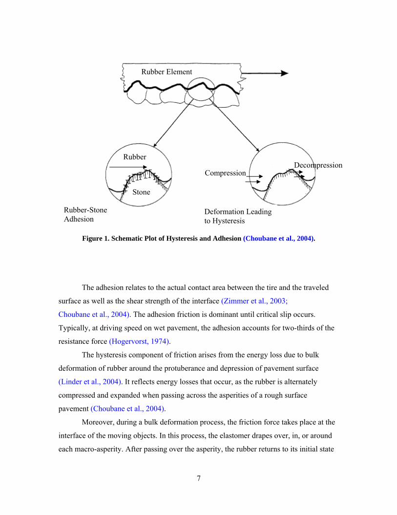
Moore (1972) in an attempt to explain the friction phenomenon between tire and
pavement, showed that frictional forces in elastomers1 comprised primarily of adhesive
and hysteresis components as shown in Figure 1 (Choubane et al., 2004). During sliding
on a wet pavement, a complex interplay between adhesion and hysteresis forces
contributes to vehicle stopping distance.
Intermolecular binding or adherence at the surface level creates the adhesive
component of friction. As the micro-asperities or surface irregularities of the two surfaces
are exposed to each other, Vander Waals or dipole forces provide an attractive force
keeping the two asperities together and prevent further movement (Dewey et al., 2001;
Person, 1998).
1 An elastomer is a polymer that shows elastic behavior (e.g., rubber).
7
Figure 1. Schematic Plot of Hysteresis and Adhesion (Choubane et al., 2004).
The adhesion relates to the actual contact area between the tire and the traveled
surface as well as the shear strength of the interface (Zimmer et al., 2003;
Choubane et al., 2004). The adhesion friction is dominant until critical slip occurs.
Typically, at driving speed on wet pavement, the adhesion accounts for two-thirds of the
resistance force (Hogervorst, 1974).
The hysteresis component of friction arises from the energy loss due to bulk
deformation of rubber around the protuberance and depression of pavement surface
(Linder et al., 2004). It reflects energy losses that occur, as the rubber is alternately
compressed and expanded when passing across the asperities of a rough surface
pavement (Choubane et al., 2004).
Moreover, during a bulk deformation process, the friction force takes place at the
interface of the moving objects. In this process, the elastomer drapes over, in, or around
each macro-asperity. After passing over the asperity, the rubber returns to its initial state
Rubber Element
Rubber
Stone
Compression Decompression
Rubber-Stone Adhesion
Deformation Leading to Hysteresis

8
but with a net loss of energy. This loss of energy contributes to the hysteresis part of
friction (Linder et al., 2004).
Several researchers tried to relate the pavement texture and friction. Yandell
emphasized the contribution of various texture scales to the hysteresis friction
(Yandell, 1971; Yandell and Sawyer, 1994; Do et al., 2000). Forster (1981) used linear
regression analysis to show that the texture shape, defined also by an average slope,
explains friction satisfactorily. Roberts (1988) showed the forces and the energy
dissipation between tire and pavement surface depend on the material properties and the
separation velocity. Kummer (1966) showed that at high-speed sliding, the hysteresis
component reaches a maximum value; while at relatively low speeds of sliding, adhesion
is at a maximum value (Dewey et al., 2001).
PAVEMENT TEXTURE
As travel safety and efficiency of the road system are of increasing importance to
state agencies, friction measurements have become an important tool in the management
of pavement surfaces (Choubane et al., 2004). The friction-related properties of a
pavement depend on its surface texture characteristics. These characteristics, as
previously stated, are known as macrotexture and microtexture (Kummer and
Meyer, 1963).
Macrotexture refers to the larger irregularities in the road surface (coarse-scale
texture) that affect the hysteresis part of the friction. These larger irregularities are
associated with voids between aggregate particles. The magnitude of this component will
depend on the size, shape, and distribution of coarse aggregates used in pavement
construction, the nominal maximum size of aggregates as well as the particular
construction techniques used in the placement of the pavement surface layer
(Noyce et al., 2005; National Asphalt Pavement Association (NAPA), 1996).
Microtexture refers to irregularities in the surfaces of the aggregate particles
(fine-scale texture) that are measured at the micron scale of harshness and are known to
be mainly a function of aggregate particle mineralogy (Noyce et al., 2005). These
irregularities make the stone particles smooth or harsh when touched. The magnitude of
microtexture depends on initial roughness on the aggregate surface and the ability of the
9
aggregate to retain this roughness against the polishing action of traffic and
environmental factors (Noyce et al., 2005; Jayawickrama et al., 1996). Microtexture
affects mainly the adhesion part of the friction (Noyce et al., 2005).
Several researchers tried to find quantitative measures to define microtexture and
macrotexture and relate them to pavement friction. Moore (1975) defined three
parameters for characterizing a surface texture: size, interspace or density, and shape.
Taneerananon and Yandell (1981) showed that, compared with the two other parameters,
the role of density is of minor importance in the water drainage mechanism. Kokkalis and
Panagouli (1999) tried to explain surface texture by using fractals. They developed a
model to relate surface depth and density to pavement friction.
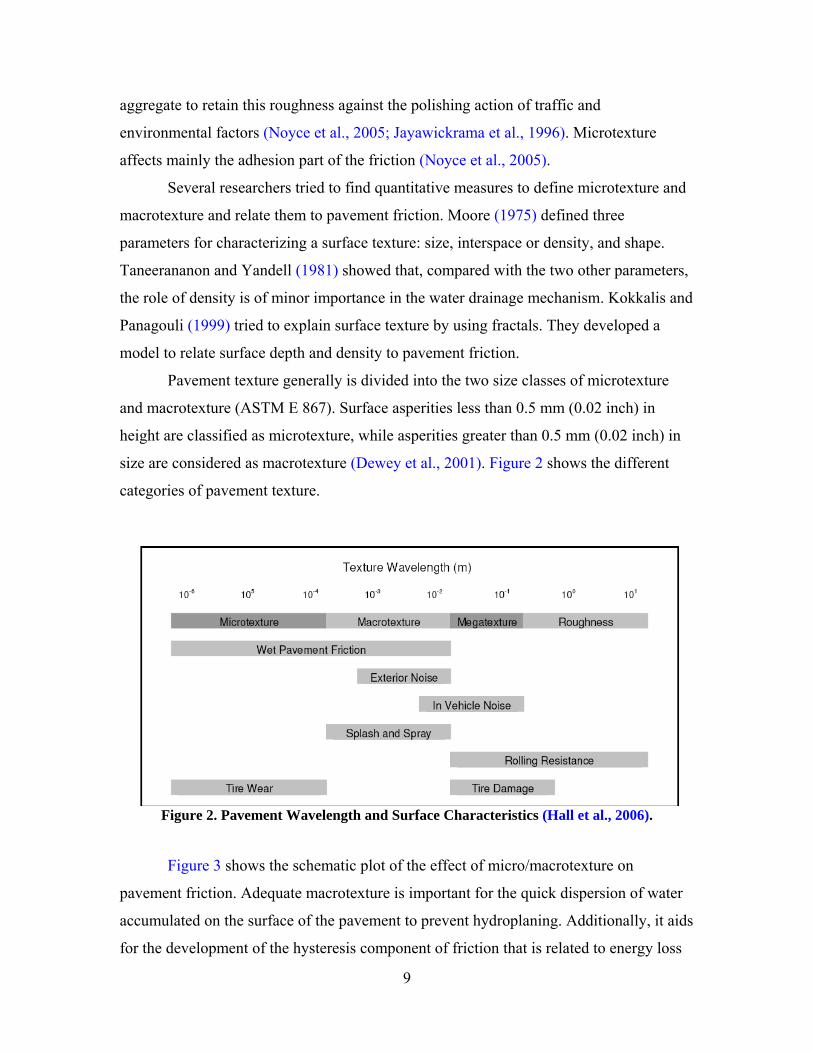
Pavement texture generally is divided into the two size classes of microtexture
and macrotexture (ASTM E 867). Surface asperities less than 0.5 mm (0.02 inch) in
height are classified as microtexture, while asperities greater than 0.5 mm (0.02 inch) in
size are considered as macrotexture (Dewey et al., 2001). Figure 2 shows the different
categories of pavement texture.
Figure 2. Pavement Wavelength and Surface Characteristics (Hall et al., 2006).
Figure 3 shows the schematic plot of the effect of micro/macrotexture on
pavement friction. Adequate macrotexture is important for the quick dispersion of water
accumulated on the surface of the pavement to prevent hydroplaning. Additionally, it aids
for the development of the hysteresis component of friction that is related to energy loss

10
as the tire deforms around macroasperities and consequently increases pavement friction
(Dewey et al., 2001; Forster, 1989; Ergun et al., 2005). Macrotexture of the pavements
could be estimated by simulating the percentage of contact points within the area of a tire
footprint on the pavement surface (Forster, 1989). Davis et al. (2002) showed that there is
a significant influence of mixture parameters on the ribbed tire skid resistance
measurements and laser profile mean texture depth. Moreover, they stated that it is
possible to predict some of the frictional properties of the wearing surface mixes based on
HMA mix design properties (Davis et al., 2002).
Bloem (1971) showed that an average texture depth of about 0.5 mm (0.02 inch)
is required as the minimum to assure the desired depletion of water from under the tire
(Bloem, 1971).
Figure 3. Schematic Plot of Microtexture/Macrotexture (Noyce et al., 2005).
Experiments conducted by Balmer (1978) showed that changes in surface textures
from about (0.02 inch to 0.12 inch) 0.5 to over 3mm resulted in a difference of 16 km/h
(10 mph) in the speed for the initiation of hydroplaning (Gardiner et al., 2004;
Balmer, 1978).
Microtexture plays a significant role in the wet road/tire contact. The size of
microasperities plays a key role in overcoming the thin water film. Existence of
microtexture is essential for squeezing the thin water film present in the contact area and
Motion
Friction
Microtexture
Macrotexture
11
generating friction forces (Do et al., 2000). Moreover, the role of microtexture is to
penetrate into thin water film present on the surface of the pavement so that the intimate
tire/pavement contact is maintained (Forster, 1989). Drainage is controlled by the shape
of microasperities (Do et al., 2000; Rhode, 1976; Taneerananon and Yandell, 1981).
Savkoor (1990) also showed that drainage of the water film between tire and pavement is
a function of amplitude and number of microasperities on a surface (Do et al., 2000).
Forster (1989) developed a parameter to account for microtexture. This parameter is a
combination of average height and average spacing between microasperities. A study by
Ong et al. (2005) showed that in the pavements comprised of coarse aggregates with high
microtexture in the range of 0.2 mm to 0.5 mm, hydroplaning occurs at a 20 percent
higher speed. This means that using materials with better microtexture reduces the chance
of hydroplaning.
Horne (1977) also stated that pavements with a good microtexture could delay
hydroplaning (Ong et al., 2005). Pelloli (1972) based his research on five different types
of surfaces and found that the amount of microtexture would affect the relationship
between friction coefficient and the water depth accumulated on the surface
(Ong et al., 2005). Moore (1975) reported a minimum water film thickness to be expelled
by microasperities in the order of 5 × 10⁻³ mm. Bond et al. (1976) reported the same order
of magnitude from visual experiments conducted to monitor the water film between a
tire and a smooth transparent plate.
Bond et al. (1976) showed how differences in surface microtexture and
macrotexture of pavement surfaces influence peak brake coefficients of a standard test
tire (Johnsen, 1997). Leu and Henry (1978) demonstrated how skid resistance tests taken
from different pavement surfaces are different based on their microtexture and
macrotexture. Horne and Buhlmann (1983), however, showed the surface friction
measurements are poorly related to pavement texture measurements (Johnsen, 1997).
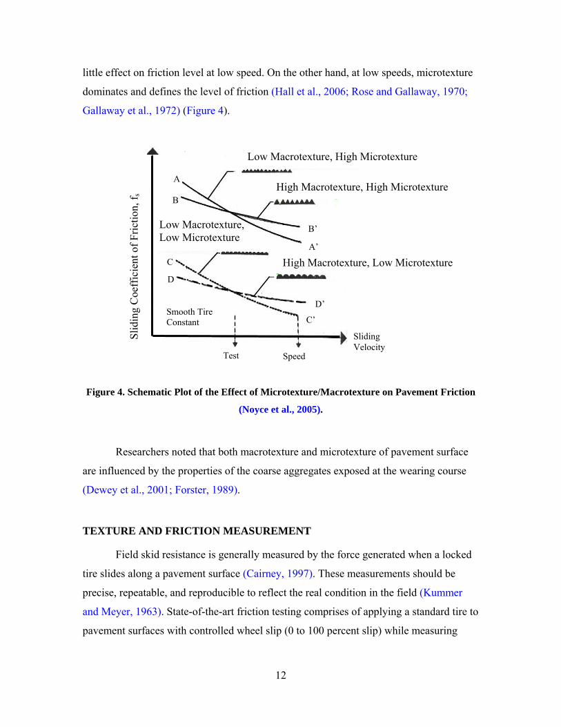
Hogervorst (1974) reported that the change of skid resistance with vehicle speed
depends on both microtexture and macrotexture. Microtexture defines the magnitude of
skid resistance, and macrotexture will control the slope of skid resistance reduction as
speed increases. Moreover, macrotexture affects the skid resistance of pavements at high
speed by reducing the friction-speed gradient and facilitating the drainage of water. It has
12
little effect on friction level at low speed. On the other hand, at low speeds, microtexture
dominates and defines the level of friction (Hall et al., 2006; Rose and Gallaway, 1970;
Gallaway et al., 1972) (Figure 4).
Figure 4. Schematic Plot of the Effect of Microtexture/Macrotexture on Pavement Friction
(Noyce et al., 2005).
Researchers noted that both macrotexture and microtexture of pavement surface
are influenced by the properties of the coarse aggregates exposed at the wearing course
(Dewey et al., 2001; Forster, 1989).
TEXTURE AND FRICTION MEASUREMENT
Field skid resistance is generally measured by the force generated when a locked
tire slides along a pavement surface (Cairney, 1997). These measurements should be
precise, repeatable, and reproducible to reflect the real condition in the field (Kummer
and Meyer, 1963). State-of-the-art friction testing comprises of applying a standard tire to
pavement surfaces with controlled wheel slip (0 to 100 percent slip) while measuring
Test Speed li i
Sliding Velocity
Smooth Tire Constant
D’
C’
B’
A’
A
B
C
D
Low Macrotexture, High Microtexture
Low Macrotexture, Low Microtexture
High Macrotexture, Low Microtexture
High Macrotexture, High Microtexture
Slid
ing
Coe
ffic
ient
of F
rictio
n, f s

13
friction between a tire (on the wheel) and pavement (American Society for Testing and
Materials (ASTM) E274, E303, E503, E556, E670, E707) (Johnsen, 1997).
There are four main types of skid resistance measuring approaches (Kokot, 2005;
Roe et al., 1998; Permanent International Association of Road Congresses
(PIARC), 1995):
• locked wheel, where the force is measured while a 100 percent slip condition is
produced;
• sideway force, where the force is measured on a rotating wheel with a yaw angle
of 20°;
• fixed slip, where friction is measured for wheels that are constantly slipping; and
• variable slip, where devices are designed to measure at any desired slip, sweep
through a predetermined set of values, or seek the maximum friction.
In each technique, relating locked-wheel and variable-slip of tires to the rolling,
braking, or cornering, friction coefficient is measured on wet pavement surfaces
(Johnsen, 1997).
Pavement friction testing with the locked wheel tester can be conducted with
either a standard ribbed tire or a standard smooth tire (Lee et al., 2005). The most
common method is the locked-wheel braking mode, which is specified by ASTM E-274.
The concept of a skid trailer was introduced in the mid-1960s to improve the safety and
efficiency of friction testing operations (Choubane et al., 2004).
According to Saito et al. (1996), there are also some disadvantages associated
with locked-wheel testers:
• Continuous measurement of skid resistance is not possible.
• Although Kummer and Meyer (1963) showed the cost of a locked-wheel trailer is
about 90 percent of other field test methods, its initial and operating costs of the
test equipment are still high.
• Tests are conducted at only one speed so that speed dependency of skid resistance
cannot be determined without repeated measurements on the same sections of
road and different speeds.
Other types of measurement modes comprise the fixed slip, variable slip, and the
sideway force or cornering mode. In the slip mode (fixed or variable), the friction factor
14
is a function of the “slip” of the test wheel while rolling over the pavement. The sideway
mode uses a test wheel that moves at an angle to the direction of motion. The use of this
test procedure is based upon the assumption that the critical situation for skid resistance
occurs in cornering (Saito et al., 1996).
These methods are categorized as field modes. Other testing modes include
portable and laboratory testers. The most common tester is the British pendulum tester
(BPT), which is a dynamic pendulum impact-type tester and is specified in ASTM E303.
The British pendulum tester (Giles et al., 1964) is one of the simplest and cheapest
instruments used in the measurement of friction characteristics of pavement surfaces. The
BPT has the advantage of being easy to handle, both in the laboratory and in the field, but
it provides only a measure of a frictional property at a low speed (Saito et al., 1996).
Although it is widely suggested that the measurement is largely governed by the
microtexture of the pavement surface, experience has shown that the macrotexture can
also affect the measurements (Fwa et al., 2003; Lee et al., 2005). Moreover,
Fwa et al. (2003) and Liu et al. (2004) showed that the British pendulum measurements
could be affected by the macrotexture of pavement surfaces, aggregate gap width, or the
number of gaps between aggregates. It can also lead to misleading results on
coarse-textured test surfaces (Lee et al., 2005).Other researchers pointed out that the
British pendulum tester exhibited unreliable behavior when tested on coarse-textured
surfaces (Forde et al., 1976; Salt, 1977; Purushothaman et al., 1988).
The DFT is a disc-rotating-type tester that measures the friction force between the
surface and three rubber pads attached to the disc. The disc rotates horizontally at a linear
speed of about 20 to 80 km/hr under a constant load. It touches the surface at different
speeds so the DFT can measure the skid resistance at any speed in this range
(Saito et al., 1996). Studies by Saito et al. (1996) showed that there is a strong
relationship between the coefficient of friction of the DFT and the British Pendulum
Number (BPN) at each point for each measuring speed (Saito et al., 1996).
Measuring the pavement microtexture and macrotexture and relating these
measurements to pavement skid resistance has been a major concern for pavement
researchers. The practice of measuring pavement macrotexture has been a common
practice in recent years (Abe et al., 2000; Henry, 2000). Yandell et al. (1983) stated that it
15
is desirable to predict pavement surface friction with computer models by use of
laboratory measurements rather than field measurement. The use of a computer model is
motivated considering that test methods are not easily repeatable and prediction methods
will save time and money (Johnsen, 1997).
Macrotexture data is generally measured using a volumetric technique.
Essentially, this method consists of spreading a known volume of a material (sand, glass
beads, or grease) into the pavement surface and measuring the resulting area. Dividing
the initial volume by the area gives Mean Texture Depth (MTD) (Ergun et al., 2005;
Leland et al., 1968). It has been reported that the sand patch method, Silly Putty method,
and volumetric methods are burdensome to use in routine testing (Jayawickrama
et al., 1996).
Outflow Meter Test (OFT) is another method to measure pavement macrotexture
(Henry and Hegmon, 1975). The outflow meter measures relative drainage abilities of
pavement surfaces. It can also be used to detect surface wear and predict correction
measures (Moore, 1966).
The OFT is a transparent vertical cylinder that rests on a rubber annulus placed on
the pavement. Then, the water is allowed to flow into the pavement, and the required time
for passing between two marked levels in the transparent vertical cylinder is recorded.
This time indicates the ability of the pavement surface to drain water and shows how fast
it depletes from the surface. This time is reported as the outflow time and can be related
to pavement macrotexture afterwards (Abe et al., 2000).
In the past decade, significant advances have been made in laser technology and
in the computational power and speed of small computers. As a result, several systems
now available can measure macrotexture at traffic speeds. The profiles produced by these
devices can be used to compute various profile statistics such as the Mean Profile Depth
(MPD), the overall Root Mean Square (RMS) of the profile height and other parameters
that reduce the profile to a single parameter (Abe et al., 2000). The Mini-Texture-Meter
developed by British Transport and Road Research Laboratory (Jayawickrama
et al., 1996), Selcom Laser System developed by researchers at the University of Texas at
Arlington (Jayawickrama et al., 1996; Walker and Payne.,undated), and the noncontact
high speed optical scanning technique developed by the researchers at Pennsylvania State
16
University (Jayawickrama et al., 1996; Her et al., 1984) are examples of these systems.
The first two of these devices use a laser beam to scan the pavement surface and, hence,
estimate pavement texture depth. The third device makes use of a strobe band of light
with high infrared content to generate shadowgraphs. This equipment can collect data
from a vehicle moving at normal highway speeds (Jayawickrama et al., 1996).
A relatively new device for measuring MPD called the Circular Texture Meter
(CTMeter) was introduced in 1998 (Henry et al., 2000; Noyce et al., 2005). The CTMeter
is a laser-based device for measuring the MPD of a pavement at a static location. The
CTMeter can be used in the laboratory as well as in the field. It uses a laser to measure
the profile of a circle 11.2 inch (284 mm) in diameter or 35 inch (892 mm) circumference
(Abe et al., 2000). The profile is divided into eight segments of 4.4 inch (111.5 mm). The
mean depth of each segment or arc of the circle is computed according to the standard
practices of ASTM and the International Standard Organization (ISO) (Abe et al., 2000).
Testing indicated that CTMeter produced comparable results to the ASTM E965 Sand
Patch Test. Studies by Hanson and Prowell (2004) indicated that the CTMeter is more
variable than the Sand Patch Test.
There are several methods for measuring the microtexture (Do et al., 2000). In
research at Pennsylvania State University, it was found that there is a high correlation
between the zero speed intercept of the friction-speed curve of the Penn State model and
the RMS of the microtexture profile height. In addition, researchers found that the BPN
values were highly correlated to this parameter. Therefore, the BPN values could be
considered as the surrogate for microtexture measurements (Henry and Liu, 1978).
Observations of pictures of road stones taken by means of the Scanning Electron
Microscope (SEM) showed how the polishing actions, as simulated in the laboratory by
the British Accelerated Polishing Test, affected the microtexture of the aggregates
(Williams and Lees, 1970; Tourenq and Fourmaintraux, 1971; Do and Marsac, 2002). It
should be kept in mind that the test results are highly sensitive and result in a large
variability in test results. For the test results to be purely indicative of aggregate textures,
other factors need to be controlled. Coupon curvature, the arrangement of aggregate
particles in a coupon for heterogeneous materials such as gravel, the length of the contact
path, and slider load have significant effects on the results, and any change in this

17
parameters would yield misleading results (Won and Fu, 1996). The aggregates are
further polished or conditioned during slider swing; consequently, the degree of polishing
varies from aggregate type to aggregate type (Won and Fu, 1996).
Schonfeld (1974) developed a method for the Ontario Transportation Department
based on subjective assessment using photos taken from the pavement. He defined
microtexture levels from road stereo photography. Despite the fact that this method is a
subjective and global method, the attributed levels were related to microasperity size and
shape (Do et al., 2000).
Direct measurements using optic or laser devices are gaining popularity because
of their simplicity and ease of use. Forster (1981) used cameras to digitize and measure
road profile images obtained from a projection device. He developed a parameter that
combines measurements of the average height and average spacing of the microtexture
asperities. Yandell and Sawyer (1994) developed a device using almost the same
measurement principle for in-situ use. Samuels (1986) used a laser sensor to record
profiles directly. The laser system, with a measuring range of 6 mm and a spot size of
around 0.1 to 0.2 mm, was not able to detect significant differences in microtexture
between road surfaces (Do et al., 2000).
Improvements of measuring devices in recent years make the measuring
techniques faster and more reliable. New data acquisition techniques include
interferometry, structured light, various 2D profiling methods, and the Scanning Laser
Position Sensor (SLPS). Figure 5 is a chart of topographic data acquisition techniques
operating near the target scales that could be used in pavement (Johnsen, 1997).

18
Figure 5. Different Data Acquisition Methods (Johnsen, 1997).
Interferometry and the stylus profiling techniques are two different methods for
measuring topographic data at scales that cover a portion of the target scales for
determining pavement texture (Johnsen, 1997).
Structured light and the SLPS are new methods of acquiring surface topography.
These methods, however, proved to have limited functionality in measuring the surface
asperities in the full range of different surfaces elevations. The SLPS was designed
specifically for acquiring topographic data from pavement surfaces. This device is highly
portable and can be easily utilized for in-situ measurement (Johnsen, 1997).
Stereo photography is a historical tool for visual inspection of surface features
qualitatively (Schonfeld, 1974). Visual inspection requires special focusing tools and a
pair of images (stereo pair), each taken at a specific angle perpendicular to the inspected
surface. This technique can potentially be used to measure the topographic features of the
surface, but the precision is obviously limited to the utilized equipment. Digital scanning
Microtexture Macrotexture
SEM Optical Stereography
Structured Light
Stylus Profiling
ASTM E1845
ASTM E965
Interferometry
SLPS
Fast
Slow
<= 10-9 10-6 10-3 1 >= 103
Rel
ativ
e A
cqui
sitio
n Sp
eed
Scale (meter)

19
systems and computer algorithms have recently been developed to analyze the pictures
taken and generating the surface texture (Johnsen, 1997). Table 1 shows a summary
comparison between different measuring devices and the advantages and disadvantages
of each method.
The AIMS introduced by Masad et al. (2005) is one of the most recent methods
measuring the aggregate texture directly by use of a microscope and a digital image
processing technique. This technique will be discussed in the next chapter
(Masad et al., 2005).

20
Table 1. Comparison between Different Skid Resistance and Texture Measuring Techniques (McDaniel and Coree, 2003).
Device About Device
Properties
Strengths
Weaknesses
Specs/used by
British
Pendulum Tester
Pendulum arm swings over sample
Evaluates the amount of kinetic energy lost when a rubber slider attached to the pendulum arm is propelled over the test surface
Portable. Very simple. Widely used
Variable quality of results. Cumbersome and sometimes ineffective calibration. Pendulum only allows for a
ASTM E303
Michigan Laboratory Friction Tester
Rotating wheel
One wheel is brought to a speed of 40 mph and dropped onto the surface of the sample. Torque measurement is recorded before wheel stops
Good measure of the tire/surface interaction. Similar to towed friction trailer
Poor measurement of pavement macrotexture. History of use on aggregate only
MDOT
Dynamic Friction Tester
Rotating sliders
Measures the coefficient of friction
Laboratory or field measurements of microtexture
N/A
ASTM E1911
North Carolina Variable Speed Friction Tester
Pendulum type testing device
Pendulum with locked wheel smooth rubber tire at its lower end
Can simulate different vehicle speeds
Uneven pavement surfaces in the field may provide inaccurate results
ASTM E707
Pennsylvania Transportation Institute (PTI) Tester
Rubber slider
Rubber slider is propelled linearly along surface by falling weight
Tests in linear direction
Companion to Penn State reciprocating polisher. Fallen into disuse
Formerly by PTI
Sand Patch
Sand spread over circular area to fill surface voids
Measures mean texture depth over covered area
Simple
Cumbersome. Poor repeatability. Average depth only
ASTM E965
Grease Patch
Grease spread over surface
Measures mean texture depth over covered area
Simple
Cumbersome. Poor repeatability. Average depth only. Not widely used
NASA

21
Device About Device
Properties
Strengths
Weaknesses
Specs/used by
Outflow Meter
Water flows from cylinder through surface voids
Estimates average texture
Simple. Quick
For non-porous surfaces only
FHWA
Dromometer
Stylus traces surface
Lowers a tracing pin that creates a profile of the specimen surface
Can measure both microtexture and macrotexture
Can only be used on small areas of pavement
----
Surtronix 3+ Profilometer
Stylus traces profiles
Horiz. Res = 1 micrometer Vert. Res = 0.001 micrometer Traverse Length = 25.4 mm
Can read microtexture and macrotexture
Can only be used on small areas of pavement
----
Circular Track Meter
Laser based
Laser mounted on an arm that rotates on a circumference of 142 mm and measures the texture
Used with DFT Fast. Portable. Repeatable
Measures small area. Relatively new
ASTM E2157
Table 1. Comparison between Different Skid Resistance and Texture Measuring Techniques (McDaniel and Coree, 2003)(cont.)

22
SKID RESISTANCE VARIATION
Pavement skid properties or friction decreases with time if no surface distresses
occur (Lee et al., 2005). Traffic- and weather-related factors also affect the surface
microtexture and macrotexture properties of in-service pavements, and thus the pavement
friction (Flintsch et al., 2005). The following subsections describe the factors that
influence the skid resistance.
Age of the Surface
Almost all new road surfaces have high texture and skid resistance. Aggregates
used in road construction have to be resistant to crushing and abrasion to provide
adequate skid resistance (Hogervorst, 1974). Pavement texture, however, reduces over
time due to the abrasive effects of traffic. Traffic has a cumulative effect on pavement,
and it wears the pavement surface and polishes the aggregate (Flintsch et al., 2005). The
traffic wears and polishes the road pavement surface to a value that may be less than that
determined by the standard Polished Stone Value (PSV) test in the laboratory
(Perry et al., 2001). This polishing is due to the horizontal forces applied by the vehicle
tires on the pavement surface. Under these forces, the protruding aggregates are worn off,
polished, or abraded, thus reducing surface microtexture and macrotexture
(Kennedy et al., 1990; Forster, 1990; Harald, 1990; Kulakowski and Meyer, 1990;
Dewey et al., 2001). In addition, under the compacting effect of traffic, the protruding
aggregates may be embedded in the pavement structure that leads to a reduction in the
depth of macrotexture. Accordingly, an average 40 percent reduction in skid resistance
due to pavement wear has been reported (Kokkalis et al., 2002). Polishing of aggregates
also relates to traffic intensity and classification. Furthermore, commercial vehicles
contribute to most of the polishing (Colony, 1986). The geometry of the road gradients,
curves, pedestrian crossings, roundabouts, and stop and give-way controlled intersections
attract high stresses and result in more polished surfaces. Polishing relates to traffic
volumes where high volume areas require a better mixture design and construction
(Chelliah et al., 2003).
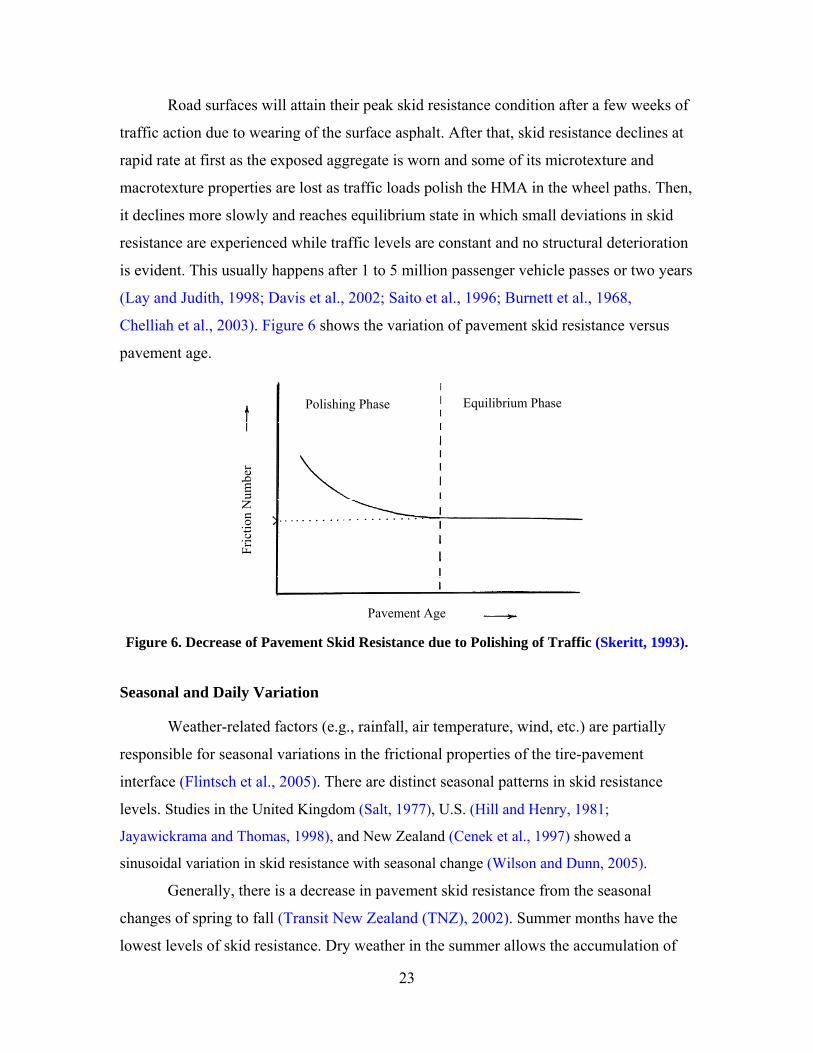
23
Road surfaces will attain their peak skid resistance condition after a few weeks of
traffic action due to wearing of the surface asphalt. After that, skid resistance declines at
rapid rate at first as the exposed aggregate is worn and some of its microtexture and
macrotexture properties are lost as traffic loads polish the HMA in the wheel paths. Then,
it declines more slowly and reaches equilibrium state in which small deviations in skid
resistance are experienced while traffic levels are constant and no structural deterioration
is evident. This usually happens after 1 to 5 million passenger vehicle passes or two years
(Lay and Judith, 1998; Davis et al., 2002; Saito et al., 1996; Burnett et al., 1968,
Chelliah et al., 2003). Figure 6 shows the variation of pavement skid resistance versus
pavement age.
Figure 6. Decrease of Pavement Skid Resistance due to Polishing of Traffic (Skeritt, 1993).
Seasonal and Daily Variation
Weather-related factors (e.g., rainfall, air temperature, wind, etc.) are partially
responsible for seasonal variations in the frictional properties of the tire-pavement
interface (Flintsch et al., 2005). There are distinct seasonal patterns in skid resistance
levels. Studies in the United Kingdom (Salt, 1977), U.S. (Hill and Henry, 1981;
Jayawickrama and Thomas, 1998), and New Zealand (Cenek et al., 1997) showed a
sinusoidal variation in skid resistance with seasonal change (Wilson and Dunn, 2005).
Generally, there is a decrease in pavement skid resistance from the seasonal
changes of spring to fall (Transit New Zealand (TNZ), 2002). Summer months have the
lowest levels of skid resistance. Dry weather in the summer allows the accumulation of
Polishing Phase Equilibrium Phase
Fric
tion
Num
ber
Pavement Age
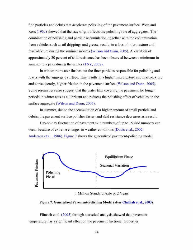
24
fine particles and debris that accelerate polishing of the pavement surface. West and
Ross (1962) showed that the size of grit affects the polishing rate of aggregates. The
combination of polishing and particle accumulation, together with the contamination
from vehicles such as oil drippings and grease, results in a loss of microtexture and
macrotexture during the summer months (Wilson and Dunn, 2005). A variation of
approximately 30 percent of skid resistance has been observed between a minimum in
summer to a peak during the winter (TNZ, 2002).
In winter, rainwater flushes out the finer particles responsible for polishing and
reacts with the aggregate surface. This results in a higher microtexture and macrotexture
and consequently, higher friction in the pavement surface (Wilson and Dunn, 2005).
Some researchers also suggest that the water film covering the pavement for longer
periods in winter acts as a lubricant and reduces the polishing effect of vehicles on the
surface aggregate (Wilson and Dunn, 2005).
In summer, due to the accumulation of a higher amount of small particle and
debris, the pavement surface polishes faster, and skid resistance decreases as a result.
Day-to-day fluctuation of pavement skid numbers of up to 15 skid numbers can
occur because of extreme changes in weather conditions (Davis et al., 2002;
Anderson et al., 1986). Figure 7 shows the generalized pavement-polishing model.
Figure 7. Generalized Pavement-Polishing Model (after Chelliah et al., 2003).
Flintsch et al. (2005) through statistical analysis showed that pavement
temperature has a significant effect on the pavement frictional properties
Pave
men
t Fric
tion
1 Million Standard Axle or 2 Years
Equilibrium Phase
Polishing Phase
Seasonal Variation
25
(Flintsch et al., 2005). In their studies, they found that for the finer wearing surface
mixes, pavement friction tends to decrease with an increase in the pavement temperature
at low speeds. At high speeds, the effect is reversed, and pavement friction tends to
increase with an increase in pavement temperatures. The temperature-dependent friction
versus speed models appears to be mix-dependent (Flintsch et al., 2005). Subhi and
Farhad (2005) in a different research study showed that both components of friction
(hysteresis, adhesion) decrease with an increase in temperature (Subhi and Farhad, 2005).
AGGREGATE POLISHING CHARACTERISTICS
The ability of an aggregate to resist the polishing action of traffic has long been
recognized as a highly important requirement for its use in pavement construction
(Bloem, 1971; Whitchurst and Goodwin, 1955; Nichols et al., 1957; Gray and
Renninger, 1965; Balmer and Colley, 1966; Csathy et al., 1968; Moore, 1969).
Coarse aggregate characteristics (e.g., angularity and resistance to wear) are
believed to have a significant role in providing sufficient skid resistance in pavements.
The desired texture is attained and retained by use of hard, irregularly shaped coarse
aggregate. Hard, polish-resistant coarse aggregate is essential to avoid reducing skid
resistance of asphalt surface (Bloem, 1971). The role of fine aggregate becomes
significant only when used in relatively large quantities (Shupe, 1960). Sharp, hard sand
particles are highly desirable for enhancing the adhesion component of pavement friction
(Hogervorst, 1974).
Aggregates in the asphalt mixture are polished differently based upon their
mineralogy. Aggregates have a different ability to maintain their microtexture against the
polishing action of traffic, and therefore, aggregates polish or become smoother at
different rates (McDaniel and Coree, 2003; Kowalski, 2007). It is a common practice to
assume that aggregates with lower Los Angeles (LA) abrasion loss, lower sulfate
soundness loss, lower freeze-thaw (F-T) loss, lower absorption, and higher specific
gravity have better resistance to polishing. Many researchers, however, believe that the
LA abrasion test and other physical tests (e.g., freeze and thaw test) may not yield good
predictions of field friction, and reliability of predicting aggregate field polishing

26
resistance using a single laboratory test is poor (West et al., 2001; Kowalski, 2007;
Prasanna et al., 1999).
The petrography examination is a valuable tool to understand the polishing
process and to state recommendations for the use of aggregates, offering promise of
quantitative evaluation (Do et al., 2002; Shupe 1960). Rocks containing igneous and
metamorphic constituents are susceptible less to polishing than sedimentary rocks and
could improve the overall frictional properties of pavement surface (West et al., 2001).
Synthetic aggregates, e.g., slag or expanded lightweight aggregate (fabricated by heating
natural clay), can also improve pavement frictional resistance (Roberts et al., 1996;
Wasilewska and Gardziejczyk, 2005; Kowalski, 2007).
Limestone, the most common type of aggregate used in road construction, is the
most susceptible aggregate type to polishing, produces the lowest skid resistance, and is
the main cause of slipperiness on pavements (Csathy et al., 1968). Individual limestone
based on its constituents differs considerably in its resistance to polishing. For some types
of carbonate aggregates (e.g., dolomite), polishing susceptibility was found to decrease
with an increase of clay content (West et al., 2001). Liang and Chyi (2000) found that as
the calcite and dolomite contents increase, the polish susceptibility of aggregates
decreases to a certain level. Further increases in the calcite and dolomite contents result
in a loss of polish resistance. The difference between polishing susceptibility is also
attributed to differences in their content of wear-resistant minerals, mainly silica
(Bloem, 1971). The siliceous particle content is considered to be equal to the insoluble
residue after treatment in hydrochloric acid under standardized conditions. The resistance
of limestone to polishing decreased as its purity increased (Shupe and Lounsbury, 1958).
Bloem (1971) stated that the siliceous particle content should be at least 25 percent to
have satisfactory polish resistance. Furthermore, the size of the siliceous particle is also
important and affects polishing tendencies. Bloem (1971) set the particle No. #50 as the
limit for the particles to be discounted in setting the required amount of acid-insoluble
material in aggregates. Sandstone is considered excellent in frictional properties and
exhibits higher wet-friction values because differential wear and pulling out of individual
particles under traffic contributes to the desired surface texture (Mills, 1969;

27
Stutzenberger, 1958). Sand and gravel are usually comprised of wear-resistant particles
and have desirable frictional properties (Bloem, 1971).
The sandstone group is composed of hard quartz particle cemented together with
brittle binder. The resistance of these particles against abrasion is very satisfactory
(Bloem, 1971). These particles are exposed when the cement is worn away by traffic;
therefore, this kind of aggregate has an excellent frictional performance, and its resistance
to polishing is always high. The limestone and flint groups yield the lowest resistance.
These types of aggregates have a simple fine cryptostalline structure and uniform
hardness. Other groups, such as basalt, granite, and quartzite, have intermediate
resistance against polishing. This intermediate resistance is due to the presence of altered
feldspars and shattered grains of quartz and quartzite dislodging from a more resistant
matrix. The basalt group, however, yields high resistance due to its softer mineral
composition and the proportion and hardness of secondary minerals. In groups of
indigenous rocks, the petrologic characteristics that affect resistance to polishing are
variation in hardness between the minerals and the proportion of soft minerals.
Finer-grained allotriomorphic igneous rocks have a tough, cohesive surface that will
polish considerably. Rocks with cracks and fractured in the individual mineral grains
have higher resistance since such grains are weak and dislodge from the matrix easily,
whereas finer-grained rocks tend to polish more readily (Bloem, 1971; Knill, 1960;
Chelliah et al., 2003).
Figure 8 shows four different methods by which aggregates provide texture to a
pavement surface. The first aggregate is a very hard, angular aggregate composed of a
single mineral type. This aggregate will resist polishing, but it will eventually become
less textured and more rounded. Furthermore, rocks consisting of minerals with nearly
the same hardness wore uniformly and tended to have a low resistance to polishing
(Chelliah et al., 2003).
The second aggregate type will result in nearly the same type of wear pattern as
the first, unless the crystals forming the particle are not well cemented together. The soft
mineral mass wears away quickly, exposing the hard grains and providing a harsh
surface. Before polishing the asperities of these hard grains, the aggregate matrix has
been worn out to such extent that it can no longer hold the hard particles, allowing them

28
to be dislodged so that fresh unpolished grains could be exposed (Abdul-Malak
et al., 1990; Skerritt, 1993). This continual renewal of the pavement surface is believed to
maintain good skid resistance properties. The aggregates that have coarse, angular, and
harder mineral grains uniformly distributed in a softer mineral matrix are believed to
have higher skid resistance (Kokkalis and Panagouli, 1999).
The third and fourth aggregate types will both wear in similar fashion. Both of
these aggregates are composed of a hard mineral and a weak mineral. For the fourth
method, the air voids act as the weak mineral type. As the particles are weathered, the
weak mineral will break down and release the worn hard minerals. This will expose fresh,
unweathered surfaces that will retain their texture for extended periods of time and keep
its frictional properties for a longer period (Luce, 2006).
Figure 8. Aggregate Methods for Providing Pavement Texture (Dahir, 1979).
PRE-EVALUATING OF AGGREGATE FOR USE IN ASPHALT MIXTURE
The resistance of an aggregate type against polishing is the key factor in
providing skid resistance. The use of polish-resistant coarse aggregates or other
aggregates with good frictional performance has always been considered a useful way to
Very Hard Materials
Conglomeration of Small Hard Particles
Dispersions of Hard Particles in a Softer Matrix
Materials that Fracture in an Irregular Angular Manner
Vesicular Materials
29
maintain friction above an acceptable level (Kokkalis and Panagouli, 1999). As
mentioned earlier, microtexture mainly depends on aggregate property that can be
controlled through the selection of aggregates with desirable polish-resistant
characteristics. The evaluation of the aggregates with respect to their polishing behavior
can be accomplished by using a laboratory test procedure (Noyce et al., 2005).
Several researchers tried to develop laboratory test methods to pre-evaluate the
aggregates and relate the properties of aggregates to skid resistance; however, there is
little agreement among researchers as to what engineering properties should be
considered in an aggregate to provide adequate frictional resistance at various average
daily traffic (ADT) levels.
Methods that are used for pre-evaluation of aggregates are mainly based upon
using the British Polish Value (BPV). This test, however, is believed to measure only the
microtexture of the pavement or the terminal polished value once the pavement reaches
its equilibrium skid resistance (Henry and Dahir, 1979). Recent studies performed by
Fwa et al. (2003) and Liu et al. (2004) showed the BPN value is a function of many
factors (e.g., magnitude and number of gaps between the aggregates’ coupon curvature,
the arrangement of aggregate particles in a coupon for heterogeneous materials such as
gravel, the length of the contact path, and slider load), and this test has a high variability
(Won and Fu, 1996).
Crouch et al. (1996) believed that current methods of pre-evaluating the
aggregates for asphalt surface courses such as the British Pendulum and British Polishing
Wheel and chemical or mineralogical methods are only able to classify well-performing
aggregates. They used a modified version of the American Association of State
Highways and Transportation Officials (AASHTO) standard device (AASHTO TP33) to
measure the uncompacted voids in coarse aggregates that were subjected to various times
in the LA abrasion test. Measuring the change in aggregate weight in the LA abrasion test
for various times is an indication of the aggregates, abrasion and breakage rate. By this
method, they were able to measure the angularity change indirectly. Although this
method does evaluate how the aggregates change over time, it is still considered an
indirect method, and it uses the LA test, which primarily breaks aggregates rather than
abrading them (Luce, 2006).

30
Do et al. (2000) used lasers to measure the surface profile of pavement sections to
determine the microtexture and macrotexture of the pavement. These measurements were
related to skid resistance (Luce, 2006). Gray and Renninger (1965) showed that the
polish susceptibility decreases as the presence of insoluble constituents such as silica
increases. Tourenq and Fourmaintraux (1971) proposed a formula to calculate the PSV
values of stones from their mineral hardness.
Prowell et al. (2005) suggested Micro-Deval as a surrogate to determine an
aggregate resistance to weathering and abrasion instead of a sulfate soundness test. It is
also stated that the Micro-Deval abrasion loss is related to the change in macrotexture
over time. Mahmoud (2005) recommended the use of Micro-Deval to polish aggregate
and AIMS to measure loss of texture.
Polishing techniques are part of any aggregate classification system that evaluates
the aggregate for use in the pavement surface. There are several types of polishing
equipment used in the past for polishing asphalt mixes including:
• Penn State Reciprocating Polishing Machine (ASTM E1393),
• Circular Track Polishing Machine,
• Michigan wear track, and
• The North Carolina State University (NCSU) Wear and Polishing Machine
(ASTM E660).
Among the polishing techniques mentioned above, only the Michigan wear track
is still being used while the others were discontinued. There is another type of the
Michigan wear track at Berlin Technical University called the Wehner/Schulze polishing
machine. This machine polishes flat circular specimens, and the polishing action is
simulated by three conical rubber rollers in the presence of water and grits (Dames 1990;
Kowalski, 2007).
The National Center of Asphalt Technology (NCAT) has recently developed a
new machine for polishing asphalt pavement slabs. In this machine, three rotating wheels
move around a circle with the same diameter as the DFT and CTMeter devices, making it
a suitable device for studying the effect of polishing with DFT and CTMeter. This
machine will be discussed in detail in the next section (Vollor and Hanson, 2006).
Table 2 shows comparisons between different polishing devices.
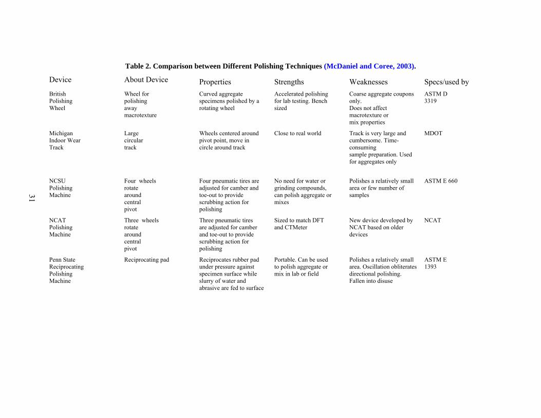
31
Table 2. Comparison between Different Polishing Techniques (McDaniel and Coree, 2003).
Device About Device Properties Strengths Weaknesses Specs/used by British Polishing Wheel
Wheel for polishing away macrotexture
Curved aggregate specimens polished by a rotating wheel
Accelerated polishing for lab testing. Bench sized
Coarse aggregate coupons only. Does not affect macrotexture or mix properties
ASTM D 3319
Michigan Indoor Wear Track
Large circular track
Wheels centered around pivot point, move in circle around track
Close to real world
Track is very large and cumbersome. Time-consuming sample preparation. Used for aggregates only
MDOT
NCSU Polishing Machine
Four wheels rotate around central pivot
Four pneumatic tires are adjusted for camber and toe-out to provide scrubbing action for polishing
No need for water or grinding compounds, can polish aggregate or mixes
Polishes a relatively small area or few number of samples
ASTM E 660
NCAT Polishing Machine
Three wheels rotate around central pivot
Three pneumatic tires are adjusted for camber and toe-out to provide scrubbing action for polishing
Sized to match DFT and CTMeter
New device developed by NCAT based on older devices
NCAT
Penn State Reciprocating Polishing Machine
Reciprocating pad
Reciprocates rubber pad under pressure against specimen surface while slurry of water and abrasive are fed to surface
Portable. Can be used to polish aggregate or mix in lab or field
Polishes a relatively small area. Oscillation obliterates directional polishing. Fallen into disuse
ASTM E 1393

32
PREDICTIVE MODELS FOR SKID RESISTANCE
Having a model to predict friction change during the lifetime of a pavement would
aid in predicting pavement performance and identifying the appropriate time for any
treatment and rehabilitation measures. Due to the complex interaction between many
factors affecting pavement skid resistance, developing such a model is not easy. Many
researchers tried to develop theoretical and empirical models to predict skid resistance.
These models range from ones based on simple laboratory tests to complicated theoretical
interaction between tire and pavement surface. These models are useful tools to predict
pavement skid resistance over its life span.
Tire/pavement models are categorized into three different categories including
(Kowalski, 2007):
• statistical-empirical that is mainly based on road-collected data with different
characteristics and statistical analysis,
• fundamental that is based on physical modeling of pavement surface and tire, and
• hybrid that is a combination of statistical and fundamental models.
Stephens and Goetz (1960) used the fineness modulus as a key factor to predict
the skid resistance of an asphalt pavement. Dahir et al. (1976) were the first to try relating
aggregate characteristics to pavement skid resistance. In their research, they found some
correlation between acid insoluble percent to field skid performance, but not enough to
support a regression equation. They were the first to propose the use of the laboratory BP
value as a surrogate for field terminal condition. They also considered the difference
between the initial and terminal laboratory BPV as a measure of polishing characteristics
of the aggregate (Luce, 2006). Henry and Dahir (1978) and Kamel and Musgrove (1981)
then used the BPV of an aggregate sample as a parameter for the prediction of a
pavement skid resistance. Henry and Dahir (1979) in other research found a relationship
between BPV and microtexture. Moreover, they introduced the concept of
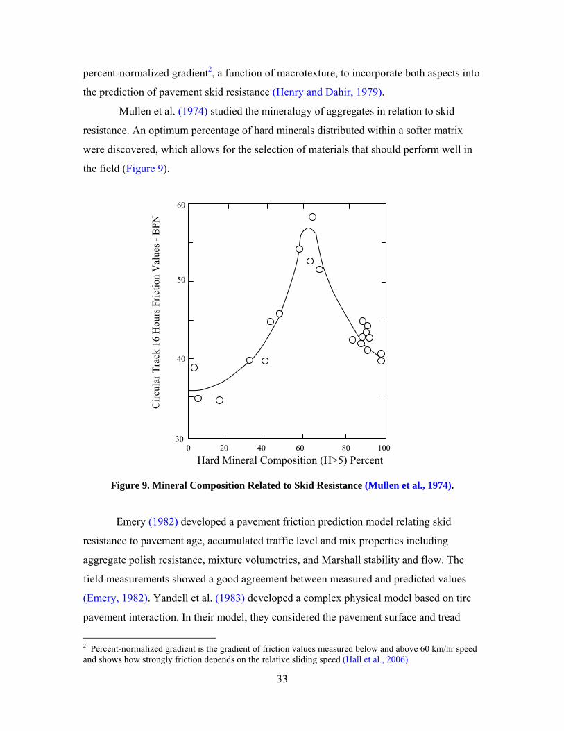
33
percent-normalized gradient2, a function of macrotexture, to incorporate both aspects into
the prediction of pavement skid resistance (Henry and Dahir, 1979).
Mullen et al. (1974) studied the mineralogy of aggregates in relation to skid
resistance. An optimum percentage of hard minerals distributed within a softer matrix
were discovered, which allows for the selection of materials that should perform well in
the field (Figure 9).
Figure 9. Mineral Composition Related to Skid Resistance (Mullen et al., 1974).
Emery (1982) developed a pavement friction prediction model relating skid
resistance to pavement age, accumulated traffic level and mix properties including
aggregate polish resistance, mixture volumetrics, and Marshall stability and flow. The
field measurements showed a good agreement between measured and predicted values
(Emery, 1982). Yandell et al. (1983) developed a complex physical model based on tire
pavement interaction. In their model, they considered the pavement surface and tread
2 Percent-normalized gradient is the gradient of friction values measured below and above 60 km/hr speed and shows how strongly friction depends on the relative sliding speed (Hall et al., 2006).
20 40 60 80 100 0 30
40
50
60
Circ
ular
Tra
ck 1
6 H
ours
Fric
tion
Val
ues -
BPN
Hard Mineral Composition (H>5) Percent

34
rubber properties as main factors affecting skid number. Field verification showed a good
agreement between predicted and measured values (Yandell et al., 1983).
Ergun et al. (2005) tried to relate pavement skid resistance and texture measurements by
use of image analysis. He also showed there is a good agreement between measured and
predicted values (Ergun et al., 2005).
Stroup-Gardner et al. (2004) found a good correlation between MPD and skid
number and developed a model to predict skid number. Ahammed and Tighe (2007)
found a close relationship between vehicle speed, surface texturing type, cumulative
traffic volume and concrete compressive strength, and concrete pavement skid resistance
and developed a model that was able to predict skid numbers for concrete pavements.
Luce et al. (2006) investigated the relationship between pavement friction and
polishing susceptibility, mix gradation, and aggregate type. Based on measuring changes
in the aggregate texture due to abrasion in Micro-Deval, they proposed a method to relate
pavement skid resistance to aggregate polishing resistance that was verified for nine
different field test sections.
INTERNATIONAL FRICTION INDEX
There are several measurement techniques throughout the world to assess
pavement skid resistance. There are many indices explaining the skid resistance of a road
including coefficient of friction, British Pendulum Number, Skid Number, Friction
Number, and International Friction Index (Henry, 2000; Kowalski, 2007). It has been a
concern how to harmonize different measurements of the skid resistance and make a
ground for comparing them. International Friction Index is a recent index that has been
developed to harmonize friction and texture measurements by means of different test
methods (Henry 1996; Henry et al. 2000; Wambold et al., 1986; Wambold et al., 1995;
Yeaman, 2005; Kowalski, 2007). This index was developed through collecting a wide
range of friction data measured by several test methods on different pavement surfaces
mainly in Spain and Belgium during an international PIARC study. In this study, a model
originated by Penn State researchers was used. In this model, two important factors
affecting pavement skid resistance were considered. The original model has the form of
(Wambold et al., 1995; Kowalski, 2007):

35
( ) Pss
eFsF−
= .0μ (1)
where:
S is sleep speed,
Fμ is friction,
F0 is a constant that relates to microtexture, and
SP is a constant that relates to macrotexture.
During the international study done by PIARC, a curve relating slip-speed was
established for each pavement section. This so-called golden curve shows the friction
experienced by a driver during emergency breaking. Then, by using proper calibration
factors, the equipment was able to predict the golden curve. It is worthwhile to know the
friction reported for each test section was at a speed of 60 km/h. The IFI is composed of
two numbers—F60 and Sp—that are calculated as follows (Wambold et al., 1995;
Kowalski, 2007).
• Speed constant (Sp) parameter is calculated based on texture measurements:
Sp = a + b Tx (2)
Where “a” and “b” are calibration factors and different for each measuring device and Tx
is a measure of pavement texture.
• The friction measurement at a slip speed FR(S) is then converted to a
measurement at 60 km/h FR(60);
( ) ( ) ⎟⎟⎠
⎞⎜⎜⎝
⎛ −
×= PSS
eSFRFR60
60 (3)
• Finally, the F(60) is recalculated by use of speed adjusted friction value FR(60)
and the following equation:
F60 = A + B FR(60) + C Tx (4)
Where; “A,” “B,” and “C” are calibration constants for a selected friction device. These
values have been standardized for each measuring device in ASTM E1960.
Two parameters used in the IFI calibrated model—wet friction at 60 km/h (F60)
and the speed constant of wet pavement friction (SP)—are indications of the average wet
coefficient of friction experienced by a driver during a locked-wheel slide at a speed of

36
60 km/h and dependence of the wet pavement friction on the sliding speed, respectively
(Cenek et al., 1997; Kowalski, 2007).
Based on the ASTM E 1960, the calibration factors for the CTMeter are
(a = 14.23 b = 89.72) and for DFT are (A = 0.081, B = 0.732). Based on these values, the
F60 and Sp could be calculated as:
PSeDFF40
20732.0081.060−
+= (5)
MPDSP 7.892.14 += (6)
where:
DF20 = wet friction number measured by DFT at the speed of 20 km/h,
MPD = MPD measured by CTMeter (mm).
These equations indicate that the effect of wet friction coefficient at 20 km/h is
more pronounced than MPD. MPD is a parameter defined by ASTM E1845 (2005) as
“the average of all of the mean segment depths of all of the segments of the profile,”
where mean segment depth is “the average value of the profile depth of the two halves of
a segment having a given base length,” and profile depth is “the difference between the
amplitude measurements of pavement macrotexture and a horizontal line through the top
of the highest peak within a given baseline.” This value could be easily read from a
CTMeter (ASTM, 2007; Kowalski, 2007).
The F60 value for the locked wheel friction trailer using a smooth tire
(A = 0.04461, B = 0.92549, and C = 0.097589) and rib tire (A = -0.02283, B = 0.60682,
and C = 0.097589) at desired speeds are (Kowalski, 2007):
TireSmoothForeSSNF PS4
.)64(01.0925.0045.0)60( ××+= (7)
TireRibForMPDeRSNF PS ×+××+−= 098.0.)64(01.0607.0023.0)60(4
(8)
where:
SN(64)S = skid number measured at test speed of 64 km/h using a smooth or rib tire
divided by 100.
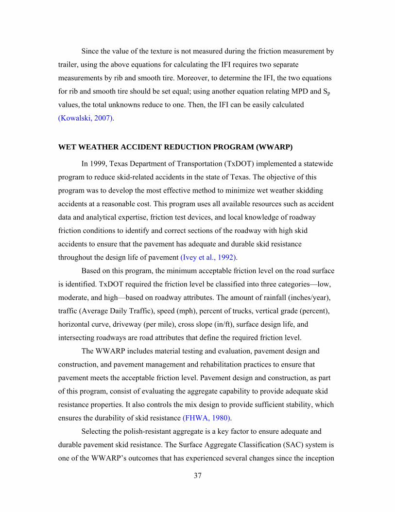
37
Since the value of the texture is not measured during the friction measurement by
trailer, using the above equations for calculating the IFI requires two separate
measurements by rib and smooth tire. Moreover, to determine the IFI, the two equations
for rib and smooth tire should be set equal; using another equation relating MPD and Sp
values, the total unknowns reduce to one. Then, the IFI can be easily calculated
(Kowalski, 2007).
WET WEATHER ACCIDENT REDUCTION PROGRAM (WWARP)
In 1999, Texas Department of Transportation (TxDOT) implemented a statewide
program to reduce skid-related accidents in the state of Texas. The objective of this
program was to develop the most effective method to minimize wet weather skidding
accidents at a reasonable cost. This program uses all available resources such as accident
data and analytical expertise, friction test devices, and local knowledge of roadway
friction conditions to identify and correct sections of the roadway with high skid
accidents to ensure that the pavement has adequate and durable skid resistance
throughout the design life of pavement (Ivey et al., 1992).
Based on this program, the minimum acceptable friction level on the road surface
is identified. TxDOT required the friction level be classified into three categories—low,
moderate, and high—based on roadway attributes. The amount of rainfall (inches/year),
traffic (Average Daily Traffic), speed (mph), percent of trucks, vertical grade (percent),
horizontal curve, driveway (per mile), cross slope (in/ft), surface design life, and
intersecting roadways are road attributes that define the required friction level.
The WWARP includes material testing and evaluation, pavement design and
construction, and pavement management and rehabilitation practices to ensure that
pavement meets the acceptable friction level. Pavement design and construction, as part
of this program, consist of evaluating the aggregate capability to provide adequate skid
resistance properties. It also controls the mix design to provide sufficient stability, which
ensures the durability of skid resistance (FHWA, 1980).
Selecting the polish-resistant aggregate is a key factor to ensure adequate and
durable pavement skid resistance. The Surface Aggregate Classification (SAC) system is
one of the WWARP’s outcomes that has experienced several changes since the inception
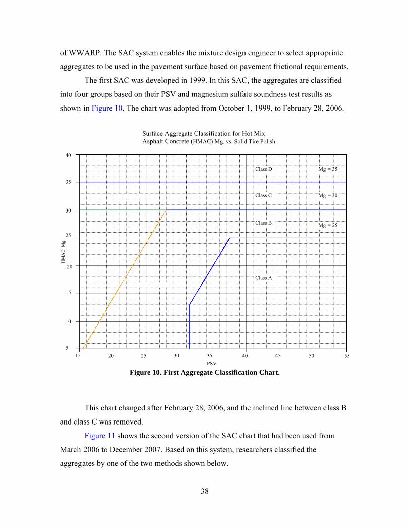
38
of WWARP. The SAC system enables the mixture design engineer to select appropriate
aggregates to be used in the pavement surface based on pavement frictional requirements.
The first SAC was developed in 1999. In this SAC, the aggregates are classified
into four groups based on their PSV and magnesium sulfate soundness test results as
shown in Figure 10. The chart was adopted from October 1, 1999, to February 28, 2006.
Figure 10. First Aggregate Classification Chart.
This chart changed after February 28, 2006, and the inclined line between class B
and class C was removed.
Figure 11 shows the second version of the SAC chart that had been used from
March 2006 to December 2007. Based on this system, researchers classified the
aggregates by one of the two methods shown below.
Surface Aggregate Classification for Hot Mix Asphalt Concrete (HMAC) Mg. vs. Solid Tire Polish
Class D
Class C
Class B
Class A
Mg = 25
Mg = 30
Mg = 35
15 20 25 30 35 40 45 50 55 5
10
15
20
25
30
5 35
40
PSV
HM
AC
Mg
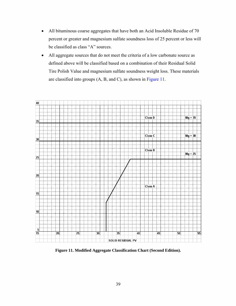
39
• All bituminous coarse aggregates that have both an Acid Insoluble Residue of 70
percent or greater and magnesium sulfate soundness loss of 25 percent or less will
be classified as class “A” sources.
• All aggregate sources that do not meet the criteria of a low carbonate source as
defined above will be classified based on a combination of their Residual Solid
Tire Polish Value and magnesium sulfate soundness weight loss. These materials
are classified into groups (A, B, and C), as shown in Figure 11.
Figure 11. Modified Aggregate Classification Chart (Second Edition).

40
In 2006, TxDOT contracted with the Texas Transportation Institute to undertake a
project to implement the AIMS in TxDOT operations. This research focused on
measuring aggregate shape characteristics. Moreover, a new method was proposed in this
research to better test aggregate resistance to polishing. This method is based on the
magnesium sulfate soundness and texture results from AIMS. It proved to be more
sensitive than the method that was being used by TxDOT. Furthermore, the new SAC
system allows the aggregates to be spread more evenly in four different categories
(Masad et al., 2006).
TxDOT began a program called Aggregate Quality Monitoring Program (AQMP)
in 1995 to provide the requirements and procedures for the Construction Division,
Materials and Pavements Section (CST/M&P) to accept aggregate products that have
demonstrated continuing quality and uniformity. In this program, TxDOT has revised the
SAC system and released the new aggregate classification system. This system has been
effective since December 2007. Based on the new system, the aggregates are classified
according to Table 3.
Table 3. Aggregate Classification Table.
Property Test Method SAC A SAC B SAC C Acid Insoluble
Residue, % min Tex-612-J 55
5-Cycle Mg, % max Tex-411-A 25 30 35 Crushed Faces, 2 or
more, % min Tex-460-A 85 85 85

41
CHAPTER III – MATERIALS AND EXPERIMENTAL DESIGN
INTRODUCTION
The research undertaken in this study examines the relationship between
aggregate properties such as angularity, texture, and pavement friction characteristics.
The results will be used to recommend a method for the selection of aggregates used in
asphalt pavement surface to ensure acceptable skid resistance. Since different aggregates
are used in different parts of the state, researchers tried to select aggregates that have
been used in projects in various locations in the state of Texas. To study the effect of mix
type, three different mixture types were selected. The following section briefly explains
the characteristics of the selected aggregates and mixture designs.
AGGREGATE SOURCES
As it was mentioned in the literature survey, aggregate type and geological
sources have a significant effect on the skid resistance of the pavement. Five different
types of aggregates were selected from:
• Beckman pit,
• Brownwood pit,
• McKelligon pit,
• Brownlee pit, and
• Fordyce pit.
It should be noted that since the frictional performance of the asphalt mixes is
mainly governed by coarse aggregates, type of coarse aggregate was considered as the
representation of that pit. For instance, in the Brownlee pit, coarse aggregate is comprised
of sandstone, and fine part is limestone from a different pit (Georgetown pit). In the
analysis, the properties of sandstone represented that of the Brownlee aggregate.
Because it is a common practice in Texas to blend soft limestone aggregates with
a polish-resistant aggregate, another combination including 50 percent sandstone and
50 percent soft limestone was also tested. Figure 12 shows the geographical location of
aggregate sources on a Texas map.
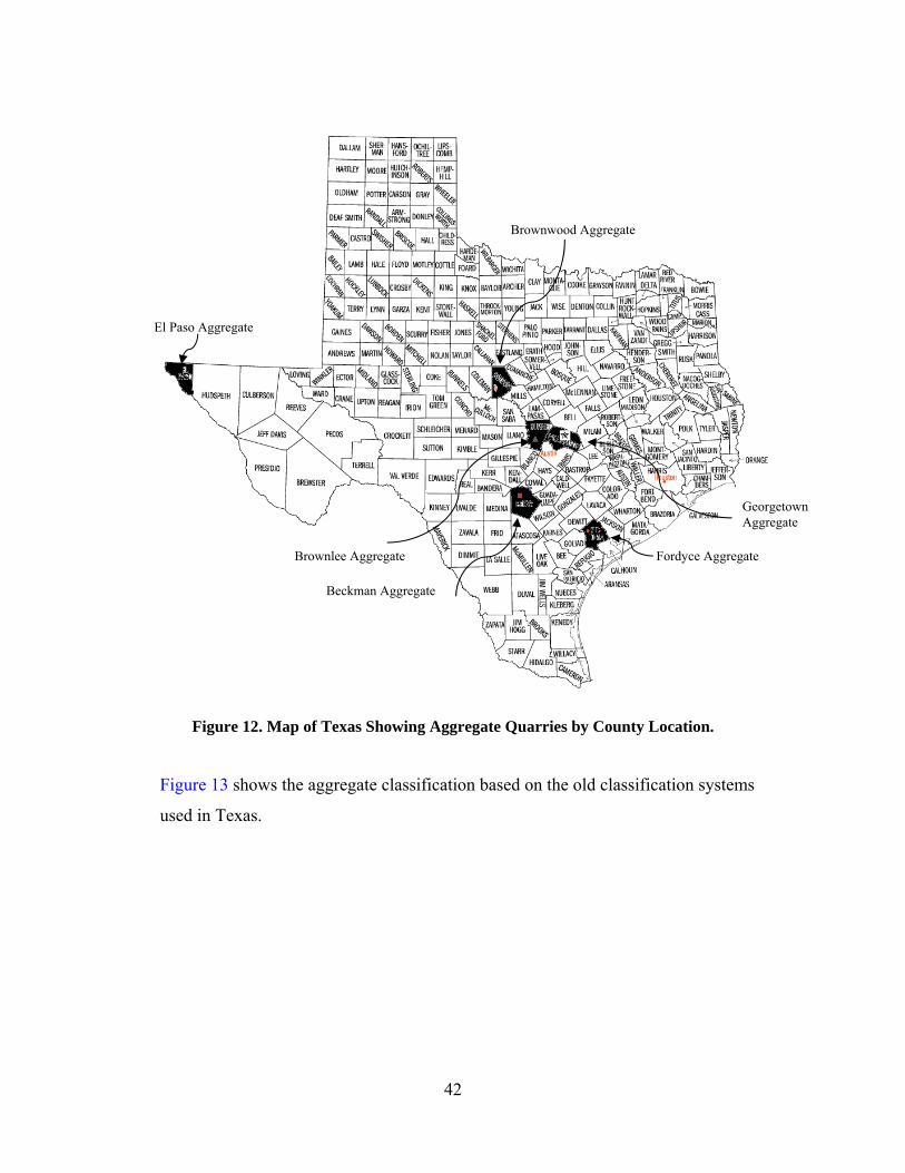
42
Figure 12. Map of Texas Showing Aggregate Quarries by County Location.
Figure 13 shows the aggregate classification based on the old classification systems
used in Texas.
El Paso Aggregate
Fordyce Aggregate
Beckman Aggregate
Georgetown Aggregate
Brownwood Aggregate
Brownlee Aggregate
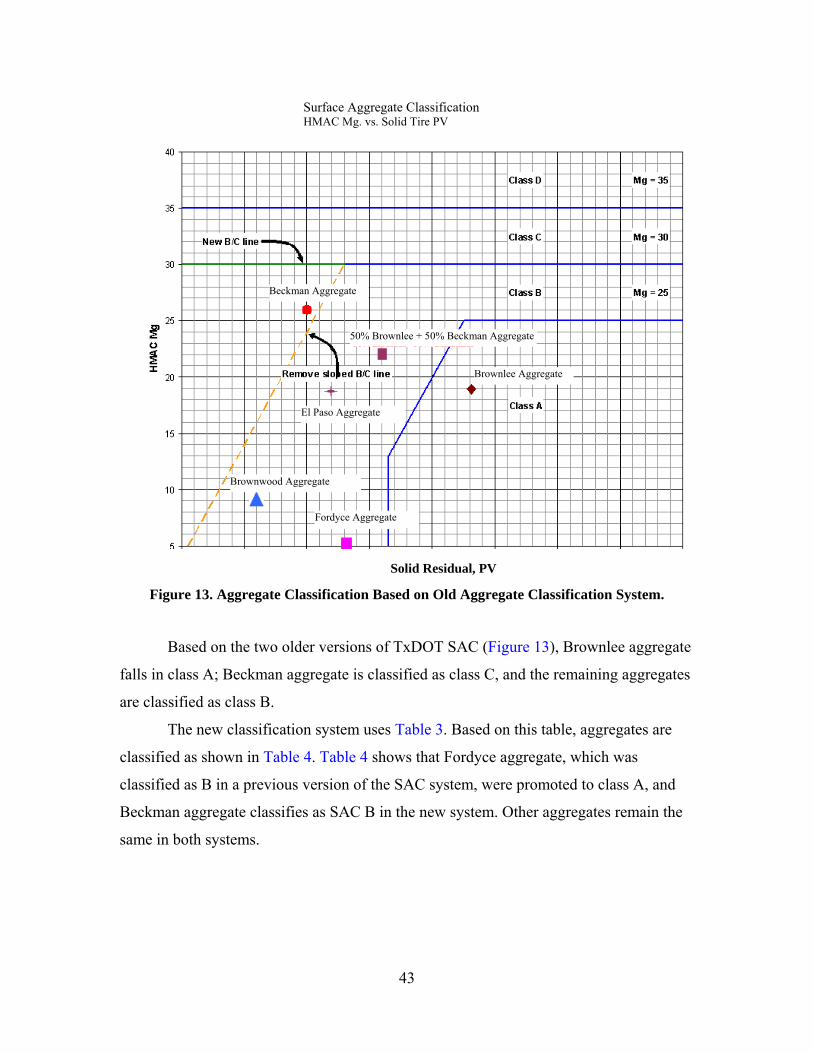
43
Figure 13. Aggregate Classification Based on Old Aggregate Classification System.
Based on the two older versions of TxDOT SAC (Figure 13), Brownlee aggregate
falls in class A; Beckman aggregate is classified as class C, and the remaining aggregates
are classified as class B.
The new classification system uses Table 3. Based on this table, aggregates are
classified as shown in Table 4. Table 4 shows that Fordyce aggregate, which was
classified as B in a previous version of the SAC system, were promoted to class A, and
Beckman aggregate classifies as SAC B in the new system. Other aggregates remain the
same in both systems.
Surface Aggregate Classification HMAC Mg. vs. Solid Tire PV
Brownwood Aggregate
Fordyce Aggregate
Beckman Aggregate
Brownlee Aggregate
50% Brownlee + 50% Beckman Aggregate
El Paso Aggregate
Solid Residual, PV
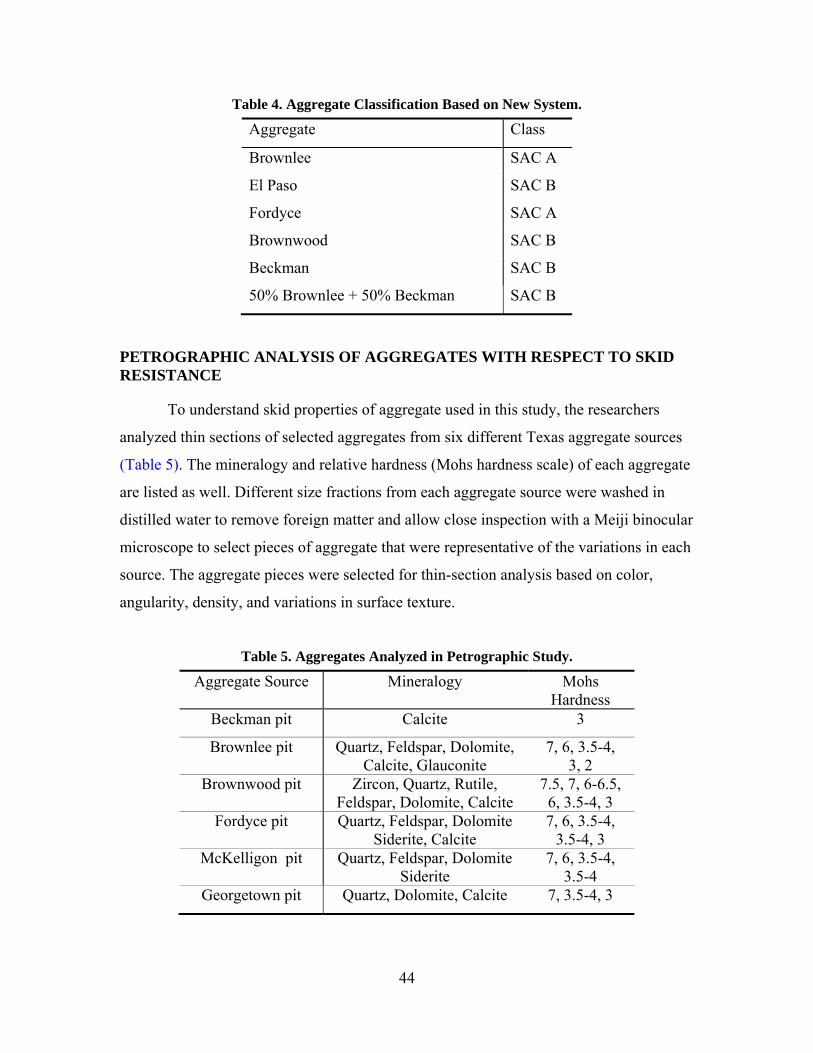
44
Table 4. Aggregate Classification Based on New System.
Aggregate Class
Brownlee SAC A
El Paso SAC B
Fordyce SAC A
Brownwood SAC B
Beckman SAC B
50% Brownlee + 50% Beckman SAC B
PETROGRAPHIC ANALYSIS OF AGGREGATES WITH RESPECT TO SKID RESISTANCE
To understand skid properties of aggregate used in this study, the researchers
analyzed thin sections of selected aggregates from six different Texas aggregate sources
(Table 5). The mineralogy and relative hardness (Mohs hardness scale) of each aggregate
are listed as well. Different size fractions from each aggregate source were washed in
distilled water to remove foreign matter and allow close inspection with a Meiji binocular
microscope to select pieces of aggregate that were representative of the variations in each
source. The aggregate pieces were selected for thin-section analysis based on color,
angularity, density, and variations in surface texture.
Table 5. Aggregates Analyzed in Petrographic Study.
Aggregate Source Mineralogy Mohs Hardness
Beckman pit Calcite 3
Brownlee pit Quartz, Feldspar, Dolomite, Calcite, Glauconite
7, 6, 3.5-4, 3, 2
Brownwood pit Zircon, Quartz, Rutile, Feldspar, Dolomite, Calcite
7.5, 7, 6-6.5, 6, 3.5-4, 3
Fordyce pit Quartz, Feldspar, Dolomite Siderite, Calcite
7, 6, 3.5-4, 3.5-4, 3
McKelligon pit Quartz, Feldspar, Dolomite Siderite
7, 6, 3.5-4, 3.5-4
Georgetown pit Quartz, Dolomite, Calcite 7, 3.5-4, 3
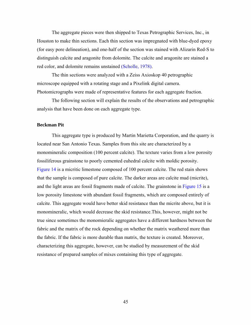
45
The aggregate pieces were then shipped to Texas Petrographic Services, Inc., in
Houston to make thin sections. Each thin section was impregnated with blue-dyed epoxy
(for easy pore delineation), and one-half of the section was stained with Alizarin Red-S to
distinguish calcite and aragonite from dolomite. The calcite and aragonite are stained a
red color, and dolomite remains unstained (Scholle, 1978).
The thin sections were analyzed with a Zeiss Axioskop 40 petrographic
microscope equipped with a rotating stage and a Pixelink digital camera.
Photomicrographs were made of representative features for each aggregate fraction.
The following section will explain the results of the observations and petrographic
analysis that have been done on each aggregate type.
Beckman Pit
This aggregate type is produced by Martin Marietta Corporation, and the quarry is
located near San Antonio Texas. Samples from this site are characterized by a
monomineralic composition (100 percent calcite). The texture varies from a low porosity
fossiliferous grainstone to poorly cemented euhedral calcite with moldic porosity.
Figure 14 is a micritic limestone composed of 100 percent calcite. The red stain shows
that the sample is composed of pure calcite. The darker areas are calcite mud (micrite),
and the light areas are fossil fragments made of calcite. The grainstone in Figure 15 is a
low porosity limestone with abundant fossil fragments, which are composed entirely of
calcite. This aggregate would have better skid resistance than the micrite above, but it is
monomineralic, which would decrease the skid resistance.This, however, might not be
true since sometimes the monomieralic aggregates have a different hardness between the
fabric and the matrix of the rock depending on whether the matrix weathered more than
the fabric. If the fabric is more durable than matrix, the texture is created. Moreover,
characterizing this aggregate, however, can be studied by measurement of the skid
resistance of prepared samples of mixes containing this type of aggregate.
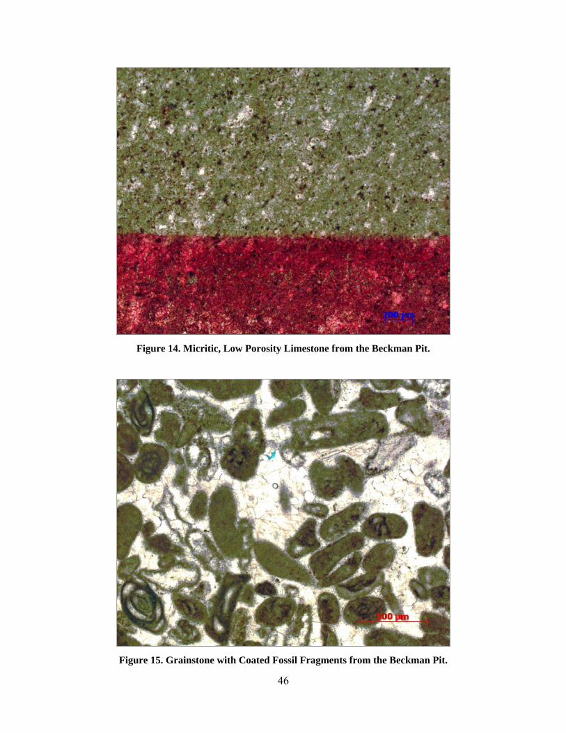
46
Figure 14. Micritic, Low Porosity Limestone from the Beckman Pit.
Figure 15. Grainstone with Coated Fossil Fragments from the Beckman Pit.

47
The limestone shown in Figure 16 has moldic (vuggy) porosity that increases its
skid resistance. However, there is very little of this material in the aggregate sample
collected. This aggregate would have a lower skid resistance due to being composed
predominantly of only one mineral.
Figure 16. Coarsely Crystalline Limestone with Moldic Pores from the Beckman Pit.
Brownlee Pit
This aggregate is a blend of sandstone and partly limestone. The sandstone is
produced by Capitol Aggregate Corporation near Marble Falls, Texas. There are
numerous rock types in this aggregate that include chert, glauconitic sandstone,
limestone, sandy limestone, dolomite, and glauconitic dolomite. Some of the aggregate
pieces are heavily weathered, and other pieces are unaltered rock. Examples include an
altered glauconitic sandstone, and fresh to highly altered dolomite. Figure 17 is an
unaltered glauconitic dolomite. The unweathered glauconite grains are dark green, and
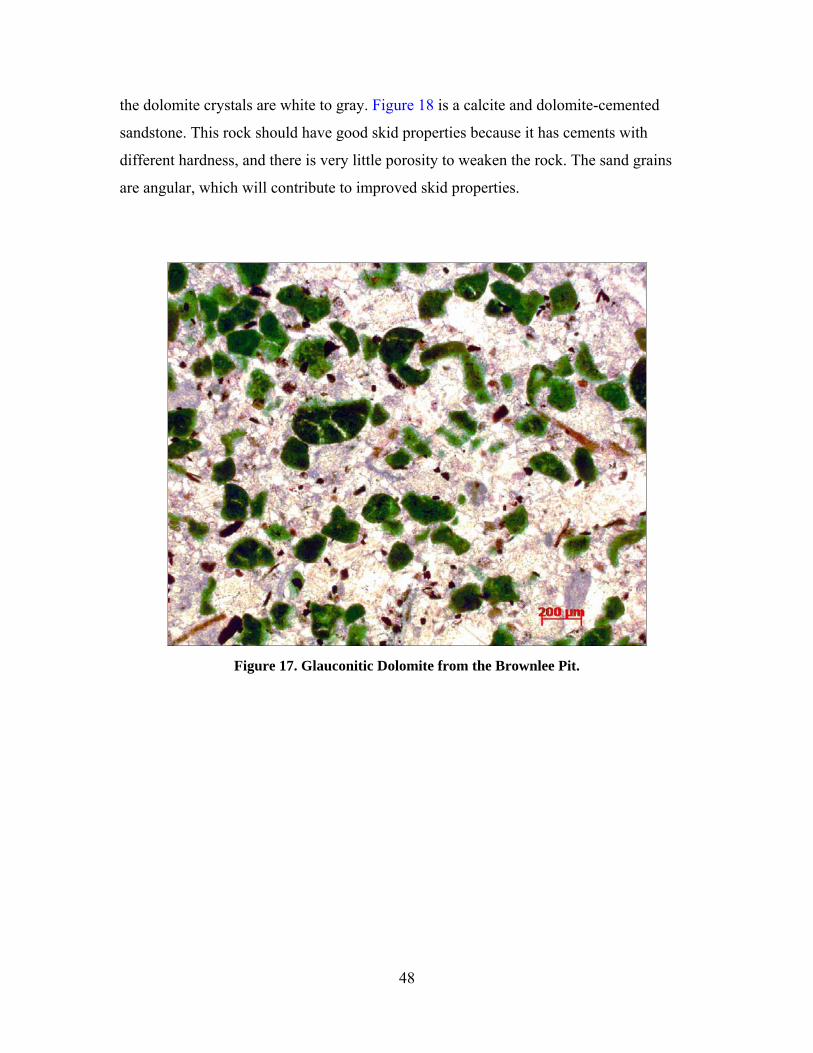
48
the dolomite crystals are white to gray. Figure 18 is a calcite and dolomite-cemented
sandstone. This rock should have good skid properties because it has cements with
different hardness, and there is very little porosity to weaken the rock. The sand grains
are angular, which will contribute to improved skid properties.
Figure 17. Glauconitic Dolomite from the Brownlee Pit.

49
Figure 18. Calcite and Dolomite-Cemented Sandstone from the Brownlee Pit.
Figure 19 shows a heavily weathered dolomite. One can see abundant pore space
(blue areas) between individual crystals in addition to many crystals being etched or
partially dissolved. The mineralogy and texture of the Brownlee Pit is very diverse. The
skid properties of this aggregate will be highly dependent on relative percentages of fresh
and heavily altered rock. The microtextural properties of the Brownlee pit is higher in the
altered rock due to continual rejuvenation of the aggregate surface due to sand being
plucked during wear. Moreover, this fresh rock may have better wear resistance
characteristics but may be less texture over time. Furthermore, a detailed laboratory study
is needed to characterize the frictional properties of this rock.
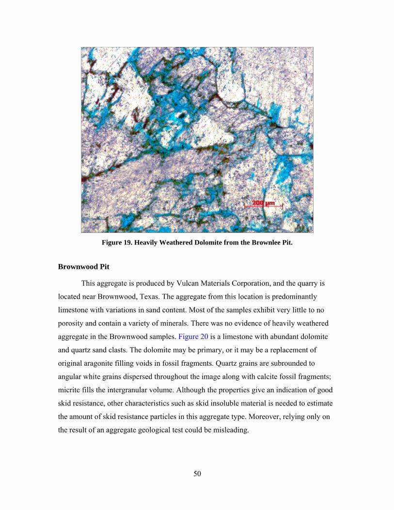
50
Figure 19. Heavily Weathered Dolomite from the Brownlee Pit.
Brownwood Pit
This aggregate is produced by Vulcan Materials Corporation, and the quarry is
located near Brownwood, Texas. The aggregate from this location is predominantly
limestone with variations in sand content. Most of the samples exhibit very little to no
porosity and contain a variety of minerals. There was no evidence of heavily weathered
aggregate in the Brownwood samples. Figure 20 is a limestone with abundant dolomite
and quartz sand clasts. The dolomite may be primary, or it may be a replacement of
original aragonite filling voids in fossil fragments. Quartz grains are subrounded to
angular white grains dispersed throughout the image along with calcite fossil fragments;
micrite fills the intergranular volume. Although the properties give an indication of good
skid resistance, other characteristics such as skid insoluble material is needed to estimate
the amount of skid resistance particles in this aggregate type. Moreover, relying only on
the result of an aggregate geological test could be misleading.

51
Figure 20. Sandy Dolomitic Limestone from the Brownwood Pit.
The image in Figure 21 is sandstone with quartz and feldspar as the dominant
constituents cemented by calcite (red) and lesser amounts of dolomite. This sample has a
heterogeneous distribution of intergranular pore space. The angularity of the detrital
grains and the carbonate cement should give this aggregate good skid property. Heavy
minerals (zircon, rutile) abound in the photomicrograph of carbonate-cemented sandstone
in Figure 22. The heavy minerals appear opaque and are concentrated in the lower half of
the figure. There is no porosity visible in this image.
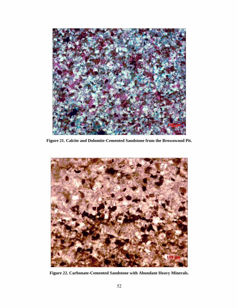
52
Figure 21. Calcite and Dolomite-Cemented Sandstone from the Brownwood Pit.
Figure 22. Carbonate-Cemented Sandstone with Abundant Heavy Minerals.

53
Fordyce Pit
This aggregate is produced by Fordyce Sand and Gravel Corporation, and the
quarry is near Victoria, Texas. Aggregates selected from the Fordyce pit samples show a
diverse origin. Rock types range from a metamorphosed sandstone to sedimentary chert,
fossiliferous limestone, silica-cemented sandstones, and dolomite. Figure 23 shows
chalcedony replacing a fossil fragment (cigar-shaped object) as well as moldic pores
derived from the dissolution of dolomite or calcite (blue). Calcite, dolomite, and siderite
are preserved in the heavily silica-cemented region in the right half of the image. This
aggregate should have good skid properties.
Figure 23. Chalcedony Replacement of Fossils and Moldic Porosity of Fordyce Pit.
The aggregate depicted in Figure 24 is composed predominantly of chalcedony
(microcrystalline quartz) with some rhombohedral calcite, dolomite, and siderite crystals
preserved. There are some rhombohedral pores developed from the dissolution of
dolomite or calcite that may help make this aggregate have good skid properties if the

54
pores are large enough. Overall, the different aggregate types found in this pit should
yield good skid resistance.
Figure 24. Chalcedony Matrix with Moldic Pores from the Fordyce Pit.
McKelligon Pit
This aggregate type is produced by Cemex Corporation, and the quarry is near
El Paso, Texas. There is some highly weathered granite in the finer fractions (< 3/8 inch),
but the aggregate is predominantly dolomite and sandy dolomite with minor fossiliferous
limestone and sandstones with dolomite and siderite cement. This aggregate should have
good skid properties provided the fine-grained limestone (Figure 26) be kept to a
minimum.
The most dominant rock type in this pit is a sand-bearing dolomite, shown in
Figure 25. The sand grains (white) are angular and composed of quartz, which will make
a rough surface when the rock is polished, so this rock should give good skid properties.
Figure 26 is a very fine-grained limestone, composed of small calcite crystals. This rock

55
would not have good skid properties because of the small crystals all composed of the
same mineral that would generate a nice uniform polish.
Figure 25. Sandy Dolomite from the El Paso, McKelligon Pit.
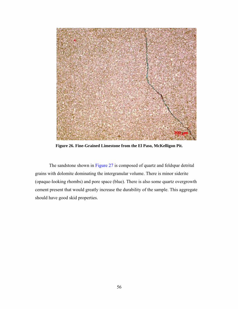
56
Figure 26. Fine-Grained Limestone from the El Paso, McKelligon Pit.
The sandstone shown in Figure 27 is composed of quartz and feldspar detrital
grains with dolomite dominating the intergranular volume. There is minor siderite
(opaque-looking rhombs) and pore space (blue). There is also some quartz overgrowth
cement present that would greatly increase the durability of the sample. This aggregate
should have good skid properties.

57
Figure 27. Dolomite and Siderite-Cemented Sandstone from the McKelligon Pit.
Figure 28 depicts one of only four granite samples. This piece is from a weathered
rock because many of the grains are etched and are being chemically altered (mottled
texture of feldspar grain in upper left corner of image). Due to the sharp contacts and
large grain sizes, and alteration granite can be considered to have satisfactory skid
resistance but a more comprehensive field and laboratory study is required to classify this
aggregate as a good skid resistant aggregate.

58
Figure 28. Cross-Polarized Light View of Altered Granite from McKelligon Pit.
Georgetown Pit
This aggregate constitutes part of aggregate called sandstone from Brownlee in
this research. The aggregate samples from Georgetown are generally not very durable,
but the poor durability can be an asset when it comes to skid performance. These
aggregates will abrade rapidly and provide a continuously rough texture. Figure 29 is an
image of a fine-grained limestone with chalcedony (microcrystalline quartz) in the lower
right side of image. This image was taken under cross-polarized light to accentuate subtle
differences in crystallography. There is a large percentage of chalcedony and chert in
these samples that will aid in skid resistance. Moldic pores (vesicles) also provide good
skid resistance in rocks with lower durability (Figure 30). One can see from this image
that the aggregate is extremely porous and poorly cemented, which will result in low
durability, but it will generally increase the skid resistance.

59
Figure 29. Fine-Grained Limestone with Chalcedony from the Georgetown Pit.
Figure 30. Moldic Pores in Limestone from the Georgetown Pit.
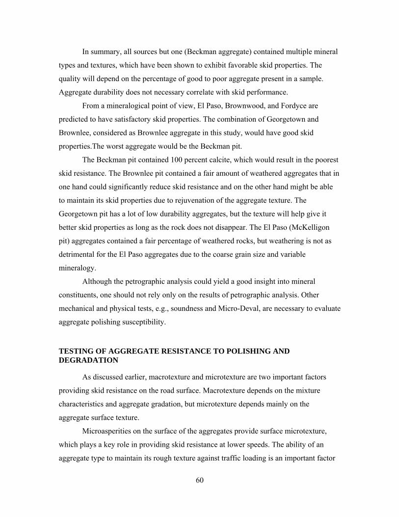
60
In summary, all sources but one (Beckman aggregate) contained multiple mineral
types and textures, which have been shown to exhibit favorable skid properties. The
quality will depend on the percentage of good to poor aggregate present in a sample.
Aggregate durability does not necessary correlate with skid performance.
From a mineralogical point of view, El Paso, Brownwood, and Fordyce are
predicted to have satisfactory skid properties. The combination of Georgetown and
Brownlee, considered as Brownlee aggregate in this study, would have good skid
properties.The worst aggregate would be the Beckman pit.
The Beckman pit contained 100 percent calcite, which would result in the poorest
skid resistance. The Brownlee pit contained a fair amount of weathered aggregates that in
one hand could significantly reduce skid resistance and on the other hand might be able
to maintain its skid properties due to rejuvenation of the aggregate texture. The
Georgetown pit has a lot of low durability aggregates, but the texture will help give it
better skid properties as long as the rock does not disappear. The El Paso (McKelligon
pit) aggregates contained a fair percentage of weathered rocks, but weathering is not as
detrimental for the El Paso aggregates due to the coarse grain size and variable
mineralogy.
Although the petrographic analysis could yield a good insight into mineral
constituents, one should not rely only on the results of petrographic analysis. Other
mechanical and physical tests, e.g., soundness and Micro-Deval, are necessary to evaluate
aggregate polishing susceptibility.
TESTING OF AGGREGATE RESISTANCE TO POLISHING AND DEGRADATION
As discussed earlier, macrotexture and microtexture are two important factors
providing skid resistance on the road surface. Macrotexture depends on the mixture
characteristics and aggregate gradation, but microtexture depends mainly on the
aggregate surface texture.
Microasperities on the surface of the aggregates provide surface microtexture,
which plays a key role in providing skid resistance at lower speeds. The ability of an
aggregate type to maintain its rough texture against traffic loading is an important factor
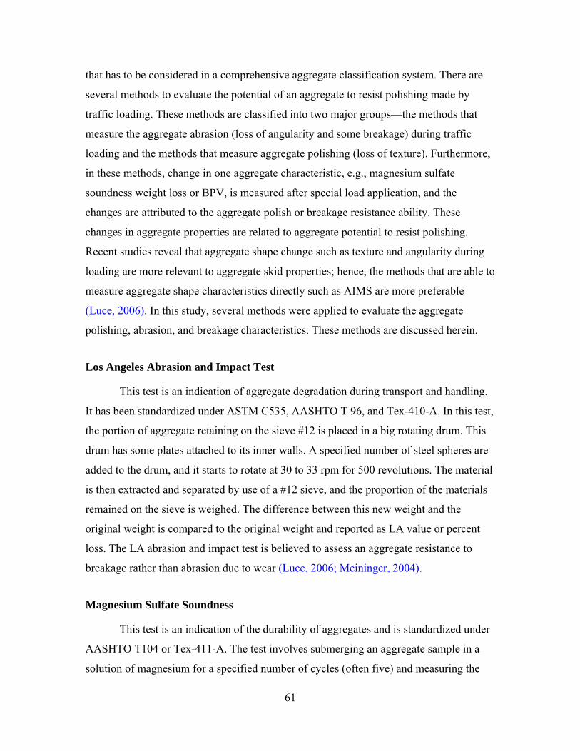
61
that has to be considered in a comprehensive aggregate classification system. There are
several methods to evaluate the potential of an aggregate to resist polishing made by
traffic loading. These methods are classified into two major groups—the methods that
measure the aggregate abrasion (loss of angularity and some breakage) during traffic
loading and the methods that measure aggregate polishing (loss of texture). Furthermore,
in these methods, change in one aggregate characteristic, e.g., magnesium sulfate
soundness weight loss or BPV, is measured after special load application, and the
changes are attributed to the aggregate polish or breakage resistance ability. These
changes in aggregate properties are related to aggregate potential to resist polishing.
Recent studies reveal that aggregate shape change such as texture and angularity during
loading are more relevant to aggregate skid properties; hence, the methods that are able to
measure aggregate shape characteristics directly such as AIMS are more preferable
(Luce, 2006). In this study, several methods were applied to evaluate the aggregate
polishing, abrasion, and breakage characteristics. These methods are discussed herein.
Los Angeles Abrasion and Impact Test
This test is an indication of aggregate degradation during transport and handling.
It has been standardized under ASTM C535, AASHTO T 96, and Tex-410-A. In this test,
the portion of aggregate retaining on the sieve #12 is placed in a big rotating drum. This
drum has some plates attached to its inner walls. A specified number of steel spheres are
added to the drum, and it starts to rotate at 30 to 33 rpm for 500 revolutions. The material
is then extracted and separated by use of a #12 sieve, and the proportion of the materials
remained on the sieve is weighed. The difference between this new weight and the
original weight is compared to the original weight and reported as LA value or percent
loss. The LA abrasion and impact test is believed to assess an aggregate resistance to
breakage rather than abrasion due to wear (Luce, 2006; Meininger, 2004).
Magnesium Sulfate Soundness
This test is an indication of the durability of aggregates and is standardized under
AASHTO T104 or Tex-411-A. The test involves submerging an aggregate sample in a
solution of magnesium for a specified number of cycles (often five) and measuring the

62
weight loss afterwards. According to the standard procedure for performing this test, the
aggregate sample is dried and placed in the magnesium solution for 18 hours. Then, it is
removed from the solution and dried again at oven temperature. This process is repeated
five times; then, the loss of aggregate weight is reported.
British Pendulum Test
The British Polish Value is a measure of aggregate surface texture and shows how
rough the aggregate surface is. This test has been standardized under ASTM E3033-93
and Tex-438-A. The test was discussed in detail in Chapter II.
Micro-Deval Test
This test is used to evaluate aggregate capability to resist abrasion in a wet
environment. The test method originated in France in 1960 and was accepted as the
European Union standard afterwards. The first use of this method was in Canada by the
Ontario Ministry of Transportation and adopted by AASHTO under the
AASHTO T 327-05 test method entitled “Standard Test Method for Resistance of Coarse
Aggregate to Degradation by Abrasion in the Micro-Deval Apparatus”
(Meininger, 2004). In this test, the durability and aggregate resistance to abrasion in the
presence of water is evaluated. Moreover, this test evaluates how aggregates degrade
when tumbled in a rotating steel container with steel balls in a wet environment (Cooley
and James, 2003; Meininger, 2004). This test method has been adopted by TxDOT in the
Tex-461-A standard procedure. In this test, a steel container is loaded with 5000 grams of
steel balls and 1500 grams of an aggregate sample in the range of 4.75 mm to 16 mm and
2000 ml tap water. This material is subjected to 9600 to 12,000 revolutions, and the
sample weight loss (weight of aggregate passed #16 sieve size) is calculated and reported.
Figure 31 shows the Micro-Deval apparatus, and Figure 32 shows the schematic
mechanism of aggregate degradation.
63
Figure 31. Micro-Deval Apparatus.
Figure 32. Mechanism of Aggregate and Steel Balls Interaction in Micro-Deval Apparatus.
This test addresses the aggregate resistance to abrasion better than other tests such
as the LA abrasion test specifically in base and HMA materials where stone-to-stone
interaction in a wet condition is more important. Moreover, the wet environment of the
Micro-Deval is believed to simulate the field condition (Rogers, 1991). Furthermore,
recent studies show that this method is more repeatable and reproducible than the other
aggregate degradation tests such as the magnesium sulfate soundness test
(Jayawickrama et al., 2006).
64
Aggregate Imaging System
The AIMS is an automated aggregate imaging system to characterize aggregate
shape characteristics. This system determines the angularity, shape, and texture of coarse
aggregate as well as the shape and angularity of fine aggregates based on a scanning
system and digital image processing. Masad et al. (2005) showed that there is no operator
bias associated with this test method, and operator training for using this equipment is not
complicated. In this system, coarse aggregates are placed on a tray with 7×8 grid points,
and fine aggregates are spread uniformly on the tray with 20×20 grid points. Then, a
digital camera with a predefined zoom level takes digital pictures of the aggregates. This
system is also equipped with back-lighting and top-lighting units that can provide enough
light intensity to capture a clear image of the aggregates. Three measures of aggregate
shape properties are calculated based on these 2-D images taken from aggregates.
Aggregate texture that shows the aggregate surface microasperities is measured
by use of wavelet theory and presented as a texture index. Aggregate angularity described
as a deviation from a perfect circle shows the irregularities on the aggregate surface on
the macro level. Angularity is calculated by use of the gradient method and presented as
an angularity index. Sphericity is another index that is extracted from digital images of
aggregates. This index simply shows how close the aggregate is to a perfect sphere. The
system is a result of a very comprehensive study being done in Texas A&M University,
and all details and analysis procedures have been documented in Al-Rousan’s Ph.D.
dissertation (Al-Rousan, 2004). Figure 33 is a schematic view of the AIMS system.
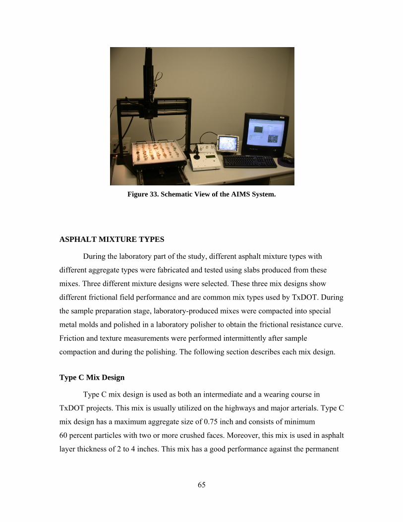
65
Figure 33. Schematic View of the AIMS System.
ASPHALT MIXTURE TYPES
During the laboratory part of the study, different asphalt mixture types with
different aggregate types were fabricated and tested using slabs produced from these
mixes. Three different mixture designs were selected. These three mix designs show
different frictional field performance and are common mix types used by TxDOT. During
the sample preparation stage, laboratory-produced mixes were compacted into special
metal molds and polished in a laboratory polisher to obtain the frictional resistance curve.
Friction and texture measurements were performed intermittently after sample
compaction and during the polishing. The following section describes each mix design.
Type C Mix Design
Type C mix design is used as both an intermediate and a wearing course in
TxDOT projects. This mix is usually utilized on the highways and major arterials. Type C
mix design has a maximum aggregate size of 0.75 inch and consists of minimum
60 percent particles with two or more crushed faces. Moreover, this mix is used in asphalt
layer thickness of 2 to 4 inches. This mix has a good performance against the permanent

66
deformation due to heavy loading and also has good skid properties. Type C mix design
has become the most common mixture design in TxDOT projects (txhotmix, 2008).
Type D Mix Design
Type D mix design is exclusively used for surface application and has a 0.5 inch
maximum aggregate size. Moreover, this mixture gives smooth riding characteristics to
the road and has good frictional properties. This mix is also used in overlay projects
(txhotmix, 2008).
Porous Friction Course
Porous Friction Course consists of an open-graded asphalt mixture containing a
large proportion of one-sized coarse aggregates typically from 0.375 to 0.5 inch in size
and a small percentage of fine aggregates. The large air content in the range of
20 ± 2 percent lets the water pass through and drain quickly; therefore, this mixture has
high skid resistance and reduces the chance of hydroplaning. Utilizing this mixture also
improves visibility and reduces water splash and spray. PFC is usually laid over a
stronger dense-graded asphalt mixture. This mixture is susceptible to moisture damage
such that in the new generation of PFCs, different kinds of additives are used
(e.g., polymers, cellulose fibers, lime) to make it more durable (txhotmix, 2008). Table 6
includes a summary of the selected mixtures and aggregates.

67
Table 6. Abbreviation Selected for Aggregates and Mix Types in This Study.
Mixture Type
Aggregate Type
Type C PFC Type D
Fordyce Aggregate CFY
Beckman Aggregate C-BK P-BK D-BK
Brownwood Aggregate C-BW P-BW
El Paso Aggregate C-EP P-EP
Brownlee Aggregate C-BL P-BL D-BL
50% Beckman + 50%
Brownlee C-BKBL D-BKBL
ASPHALT MIXTURE PREPARATION
To have a base for further comparisons, the mixture designs for each asphalt
mixture were adopted based upon a mixture design that had been used in the field. In this
regard, the mixture design for each mixture was collected by contacting TxDOT officials
and consultant engineers who were responsible for the mixture design. Tables 37 to 48 in
Appendix A show the mix design for each asphalt mixture. For two mixes—Type D with
50 percent Beckman aggregate + 50 percent Brownlee aggregate, and Brownlee—a
separate mixture design based on 4 percent air void criteria, a TxDOT mixture design
procedure for Type D mix was done. The optimum asphalt content was also estimated
and used in preparation of test specimens.
Based on the mix designs, the required amount of each aggregate type was
collected from the producer, and the gradation of each of the individual types of
aggregate quarry was determined following the ASTM C 136 (2006) specification. The
final gradation used in the production of the HMA mixes was obtained by blending
individual fractions in proportions specified in the mix design. Researchers noticed
during the blending of each bin that the final blend did not differ from the target
gradation by more than ±5 percent for each sieve size. A modified PG 76-22s binder was
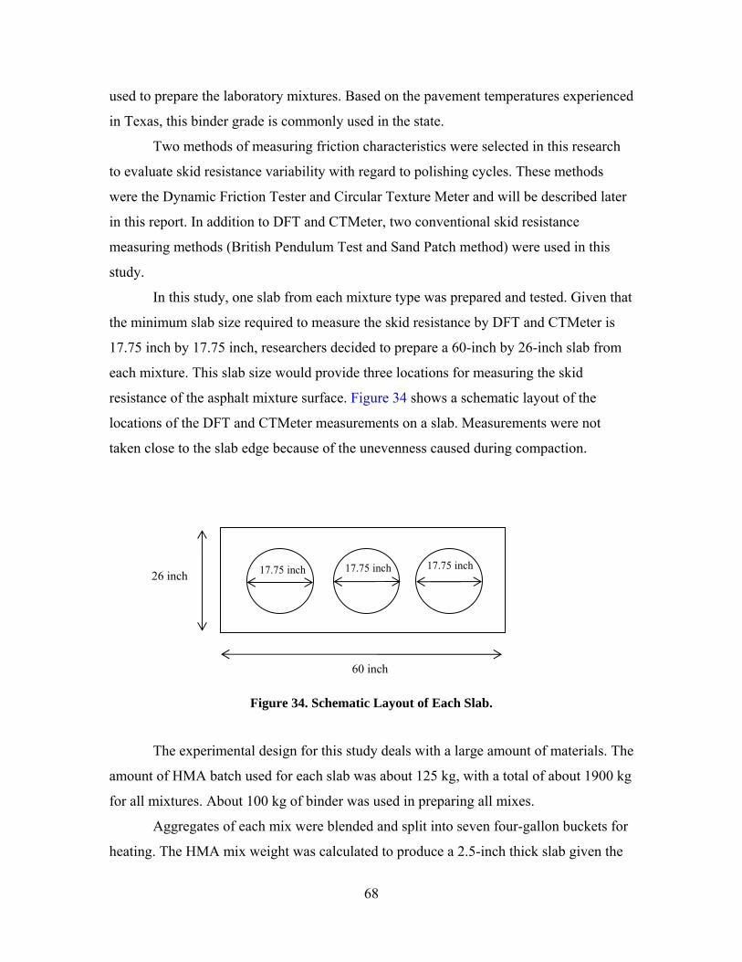
68
used to prepare the laboratory mixtures. Based on the pavement temperatures experienced
in Texas, this binder grade is commonly used in the state.
Two methods of measuring friction characteristics were selected in this research
to evaluate skid resistance variability with regard to polishing cycles. These methods
were the Dynamic Friction Tester and Circular Texture Meter and will be described later
in this report. In addition to DFT and CTMeter, two conventional skid resistance
measuring methods (British Pendulum Test and Sand Patch method) were used in this
study.
In this study, one slab from each mixture type was prepared and tested. Given that
the minimum slab size required to measure the skid resistance by DFT and CTMeter is
17.75 inch by 17.75 inch, researchers decided to prepare a 60-inch by 26-inch slab from
each mixture. This slab size would provide three locations for measuring the skid
resistance of the asphalt mixture surface. Figure 34 shows a schematic layout of the
locations of the DFT and CTMeter measurements on a slab. Measurements were not
taken close to the slab edge because of the unevenness caused during compaction.
Figure 34. Schematic Layout of Each Slab.
The experimental design for this study deals with a large amount of materials. The
amount of HMA batch used for each slab was about 125 kg, with a total of about 1900 kg
for all mixtures. About 100 kg of binder was used in preparing all mixes.
Aggregates of each mix were blended and split into seven four-gallon buckets for
heating. The HMA mix weight was calculated to produce a 2.5-inch thick slab given the
60 inch
26 inch 17.75 inch 17.75 inch 17.75 inch

69
mold volume and bulk specific gravity (Gmb). The target percent air voids was 7 percent
for Type C and Type D mixtures and 20 percent for the PFC mixture.
The four-gallon buckets containing aggregates were put into the oven one night
before compaction at the mixing temperature. The asphalt binder was also split into small
cans to achieve uniform heating. The small cans of desired asphalt type were also heated
to their mixing temperature. The heated aggregate was weighed, and the optimum asphalt
content was added to it and placed in the mixer for Type C and Type D mixtures. For the
PFC mixtures, a 15-second dry-mixing time was applied to the aggregate and fiber blend
prior to adding asphalt to have a consistent mix. The mixing was performed in a
four-gallon “bucket type” laboratory mixer. In both cases, mixing continued to assure a
consistent mix with a uniform asphalt film thickness around each particle. During the
mixing time, a long spatula was used to aid the mixing process and scratch off any fines
and asphalt from the side of the container. This process helped to obtain a uniform mix
with minimum segregation and total number of uncoated aggregate (Vollor and
Hanson, 2006). After mixing, the mix samples were placed into an oven in separate
batches, and the mixes were conditioned for two hours at the compaction temperature
(145°C or 293oF) according to the AASHTO R 30 (2002) specification.
A specially developed laboratory compaction procedure was adopted to prepare
the specimens in this study. Since the large size of the slabs limits the use of conventional
compaction methods (e.g., kneading compactor), researchers decided to use a
walk-behind roller compactor. This equipment has been successfully utilized in the field
and is fast. A metal mold was fabricated to confine the mix during the compaction. This
mold consists of five metal pieces bolted together and forms a frame to confine the
mixture. In this form, a 66 inch × 33 inch baseplate is underlying two 2.36 inch ×
2.36 inch L-shape sections as the walls. Two ramp-shape metal pieces were also
fabricated and mounted at both ends of the frame to facilitate moving of the walk-behind
roller compactor up to the frame. Figure 35 shows the schematic of the mold used to
confine the mixture during compaction.
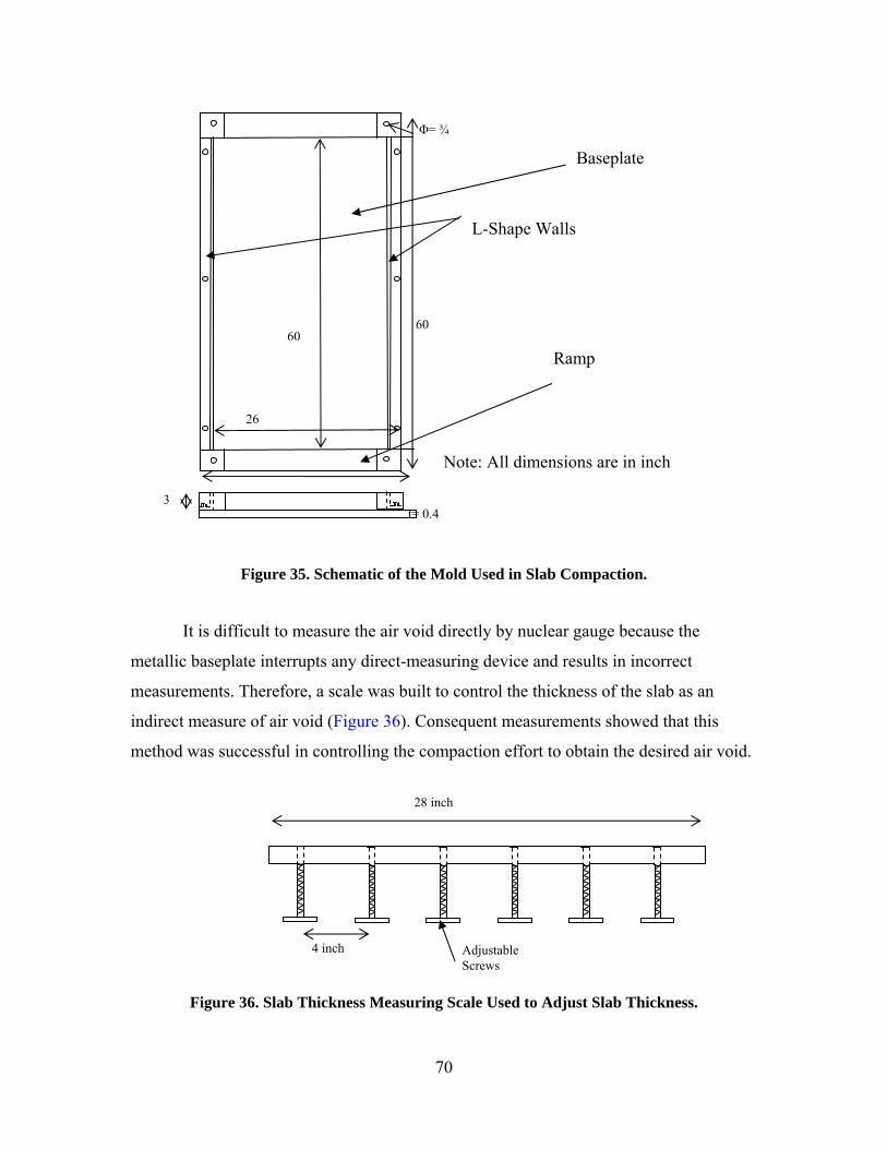
70
Figure 35. Schematic of the Mold Used in Slab Compaction.
It is difficult to measure the air void directly by nuclear gauge because the
metallic baseplate interrupts any direct-measuring device and results in incorrect
measurements. Therefore, a scale was built to control the thickness of the slab as an
indirect measure of air void (Figure 36). Consequent measurements showed that this
method was successful in controlling the compaction effort to obtain the desired air void.
Figure 36. Slab Thickness Measuring Scale Used to Adjust Slab Thickness.
28 inch
4 inch Adjustable Screws
Note: All dimensions are in inch
26
60
Φ= ¾
60
t= 0.4 3
Baseplate
L-Shape Walls
Ramp
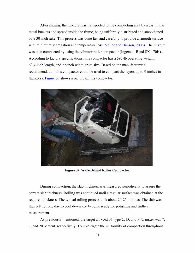
71
After mixing, the mixture was transported to the compacting area by a cart in the
metal buckets and spread inside the frame, being uniformly distributed and smoothened
by a 30-inch rake. This process was done fast and carefully to provide a smooth surface
with minimum segregation and temperature loss (Vollor and Hanson, 2006). The mixture
was then compacted by using the vibrator roller compactor (Ingersoll-Rand SX-170H).
According to factory specifications, this compactor has a 595-lb operating weight,
60.4-inch length, and 22-inch width drum size. Based on the manufacturer’s
recommendation, this compactor could be used to compact the layers up to 9 inches in
thickness. Figure 37 shows a picture of this compactor.
Figure 37. Walk-Behind Roller Compactor.
During compaction, the slab thickness was measured periodically to assure the
correct slab thickness. Rolling was continued until a regular surface was obtained at the
required thickness. The typical rolling process took about 20-25 minutes. The slab was
then left for one day to cool down and become ready for polishing and further
measurement.
As previously mentioned, the target air void of Type C, D, and PFC mixes was 7,
7, and 20 percent, respectively. To investigate the uniformity of compaction throughout
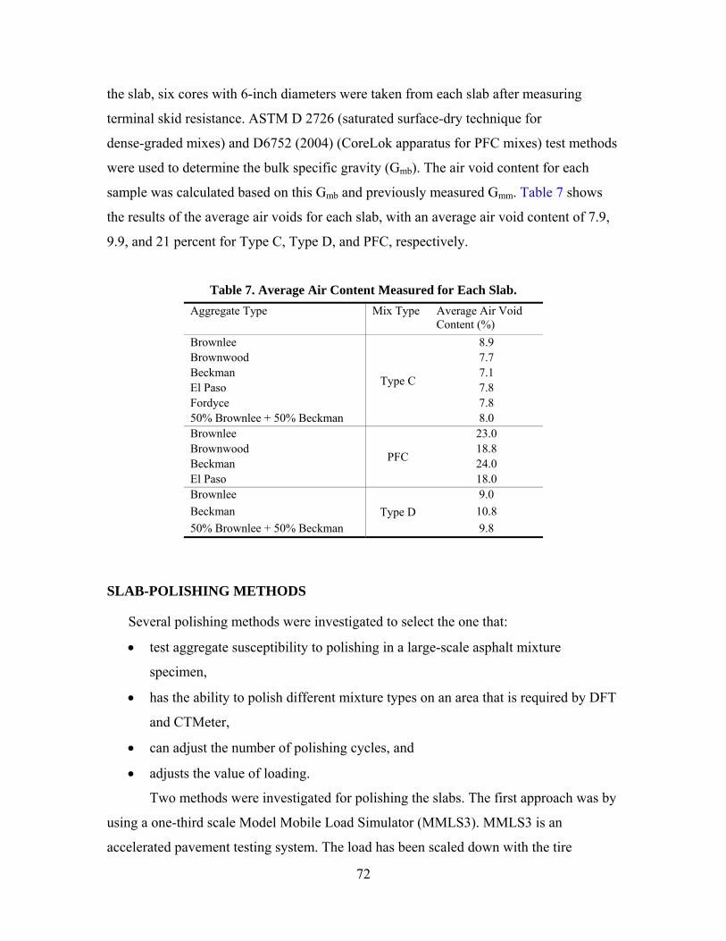
72
the slab, six cores with 6-inch diameters were taken from each slab after measuring
terminal skid resistance. ASTM D 2726 (saturated surface-dry technique for
dense-graded mixes) and D6752 (2004) (CoreLok apparatus for PFC mixes) test methods
were used to determine the bulk specific gravity (Gmb). The air void content for each
sample was calculated based on this Gmb and previously measured Gmm. Table 7 shows
the results of the average air voids for each slab, with an average air void content of 7.9,
9.9, and 21 percent for Type C, Type D, and PFC, respectively.
Table 7. Average Air Content Measured for Each Slab. Aggregate Type Mix Type Average Air Void
Content (%) Brownlee
Type C
8.9 Brownwood 7.7 Beckman 7.1 El Paso 7.8 Fordyce 7.8 50% Brownlee + 50% Beckman 8.0 Brownlee
PFC
23.0 Brownwood 18.8 Beckman 24.0 El Paso 18.0 Brownlee
Type D 9.0
Beckman 10.8 50% Brownlee + 50% Beckman 9.8
SLAB-POLISHING METHODS
Several polishing methods were investigated to select the one that:
• test aggregate susceptibility to polishing in a large-scale asphalt mixture
specimen,
• has the ability to polish different mixture types on an area that is required by DFT
and CTMeter,
• can adjust the number of polishing cycles, and
• adjusts the value of loading.
Two methods were investigated for polishing the slabs. The first approach was by
using a one-third scale Model Mobile Load Simulator (MMLS3). MMLS3 is an
accelerated pavement testing system. The load has been scaled down with the tire

73
pressure at the same level of real traffic loading. Load frequency, tire pressure,
temperature, and speed can be adjusted in this equipment (UMass, 2008). The MMLS3
consists of four rotating axles equipped with a 300-mm (11.8 inch) diameter pneumatic
tire. The load level on each tire could vary between 2.1 kN to 2.7 kN by adjusting the
suspension system. The tire pressure could be raised up to 800 kPa. This equipment is
able to apply up to 7200 loads per second (Smit et al., 2004). Figure 38 shows a picture
of the MMLS3. Slabs were compacted and placed under the MMLS3 for polishing. After
several attempts, the use of MMLS3 for polishing was discontinued due to the following
problems observed during polishing:
• The rate of polishing was very slow, and even after 200,000 cycles, the surface
was not polished significantly.
• In each turn, only one strip with a 3-inch width is polished, and to make a
measurement with the DFT and CTMeter, at least six polished strips were needed
side by side. Therefore, the polishing process was time-consuming.
• A significant amount of rutting was observed that was believed to adversely affect
the friction measurements by DFT and CTMeter.
Figure 38. Schematic View of MMLS3 (after Hugo 2005).

74
In the second method, a polishing test machine already evaluated by NCAT was
used. The results of the study by Vollor and Hanson (2006) showed that this machine has
satisfactory performance and could simulate the field condition (Vollor and
Hanson, 2006). This machine has three 8-inch × 3-inch caster wheels attached to a
turntable. These three wheels spin on an 11.188 inch diameter path; therefore, it is
possible to measure the polished area by DFT and CTMeter. It is believed that this
configuration polishes the surface of the slabs similar to the way that traffic does on a
pavement. To guide the wheels in an 11.188 inch circular track, the wheels are equipped
with ball bearings that use a mounted fixture, maintaining the wheels on the track during
the polishing time. The applied load on the wheels is variable and could be adjusted
through adding and subtracting of circular iron plates on the turning table. The turntable
is hinged to the motor shaft by use of a square shaft and can easily move up and down;
hence, this system facilitates adjusting the applied load to the wheels. Figure 39 shows
the polishing machine assembly. This system is turned by a 0.5 horsepower electrical
motor through a gearbox. The motor is equipped with a Baldor motor speed controller
that facilitates varying the rotation speed. There is also a counter system provided to
control the number of revolutions by use of an Omega digital counter and laser light
pick-up. Moreover, this system could turn off the motor by reaching a preset value for
number of revolutions. The turntable was put in a cage for safety. There is also a water
spray system included in this polisher. The spraying system consists of three 0.25 inch
PVC pipes on each side of the cage that can wash away the abraded material from the
surface and allow polishing of the slab. An electric cut-off valve attached to the water
spray system is synchronized with the Omega counter that cuts off the water after
reaching the desired revolutions (Vollor and Hanson, 2006). The original machine was
designed with the slabs inserted into the protecting cage, but in this research, the square
rod linking turntable and motor was modified so that it was possible to place the polisher
on the slab and polish it.

75
Figure 39. Polishing Machine Assembly.
TESTING OF MIXTURE RESISTANCE TO POLISHING
There is no standard test procedure for measuring pavement friction during mix
design; however, four different tests have been widely used to evaluate mixture skid
properties such as macrotexture and microtexture. These tests include: British Pendulum
skid tester (ASTM D3319-00 and E303-93 (re-approved 2003)), measuring pavement
macrotexture depth using a volumetric technique—Sand Patch Test—(ASTM E965),
measuring pavement surface frictional properties using the Dynamic Friction Tester
(E1911-98), and measuring pavement macrotexture properties using the CTMeter
(ASTM E2157-01). The following sections give a brief review of test methods (Vollor
and Hanson, 2006).
British Pendulum Skid Tester
The British Pendulum skid tester is probably the most widespread equipment in
the world to measure skid resistance. BPT was invented by Percy Sigler in the 1940s and
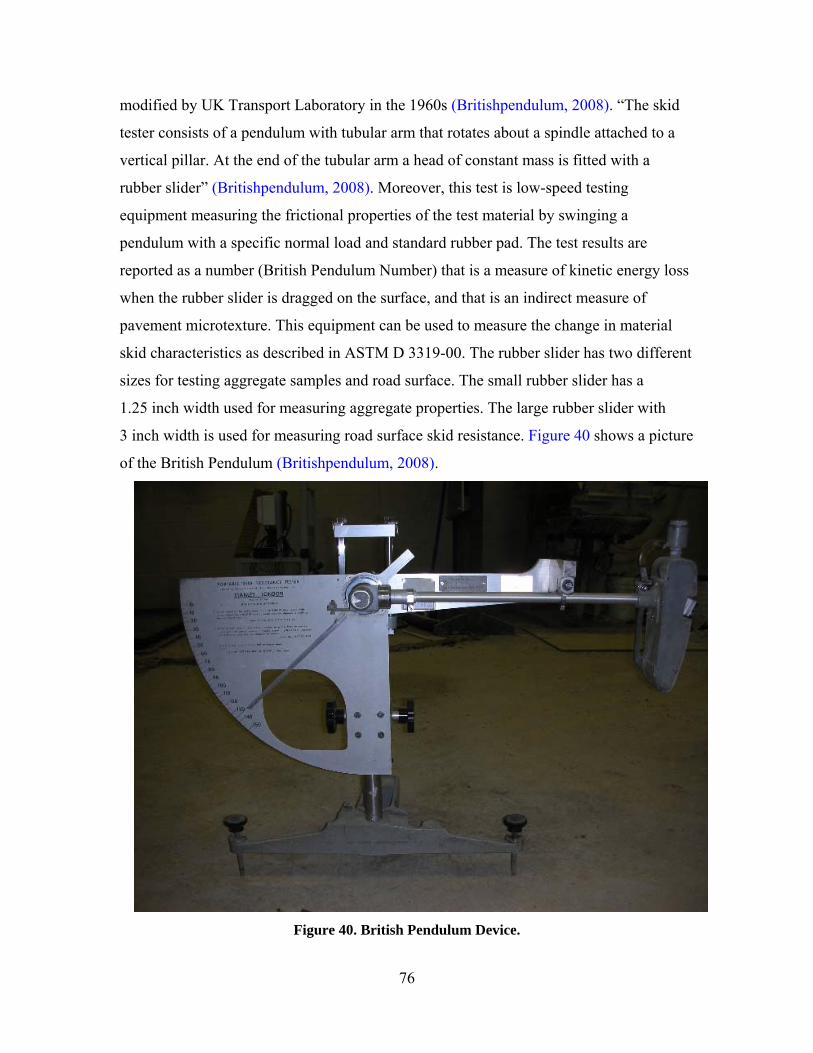
76
modified by UK Transport Laboratory in the 1960s (Britishpendulum, 2008). “The skid
tester consists of a pendulum with tubular arm that rotates about a spindle attached to a
vertical pillar. At the end of the tubular arm a head of constant mass is fitted with a
rubber slider” (Britishpendulum, 2008). Moreover, this test is low-speed testing
equipment measuring the frictional properties of the test material by swinging a
pendulum with a specific normal load and standard rubber pad. The test results are
reported as a number (British Pendulum Number) that is a measure of kinetic energy loss
when the rubber slider is dragged on the surface, and that is an indirect measure of
pavement microtexture. This equipment can be used to measure the change in material
skid characteristics as described in ASTM D 3319-00. The rubber slider has two different
sizes for testing aggregate samples and road surface. The small rubber slider has a
1.25 inch width used for measuring aggregate properties. The large rubber slider with
3 inch width is used for measuring road surface skid resistance. Figure 40 shows a picture
of the British Pendulum (Britishpendulum, 2008).
Figure 40. British Pendulum Device.
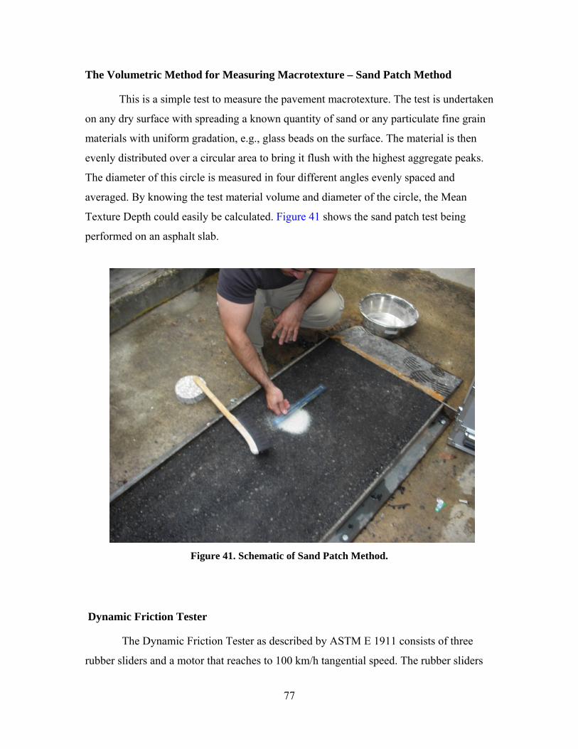
77
The Volumetric Method for Measuring Macrotexture – Sand Patch Method
This is a simple test to measure the pavement macrotexture. The test is undertaken
on any dry surface with spreading a known quantity of sand or any particulate fine grain
materials with uniform gradation, e.g., glass beads on the surface. The material is then
evenly distributed over a circular area to bring it flush with the highest aggregate peaks.
The diameter of this circle is measured in four different angles evenly spaced and
averaged. By knowing the test material volume and diameter of the circle, the Mean
Texture Depth could easily be calculated. Figure 41 shows the sand patch test being
performed on an asphalt slab.
Figure 41. Schematic of Sand Patch Method.
Dynamic Friction Tester
The Dynamic Friction Tester as described by ASTM E 1911 consists of three
rubber sliders and a motor that reaches to 100 km/h tangential speed. The rubber sliders
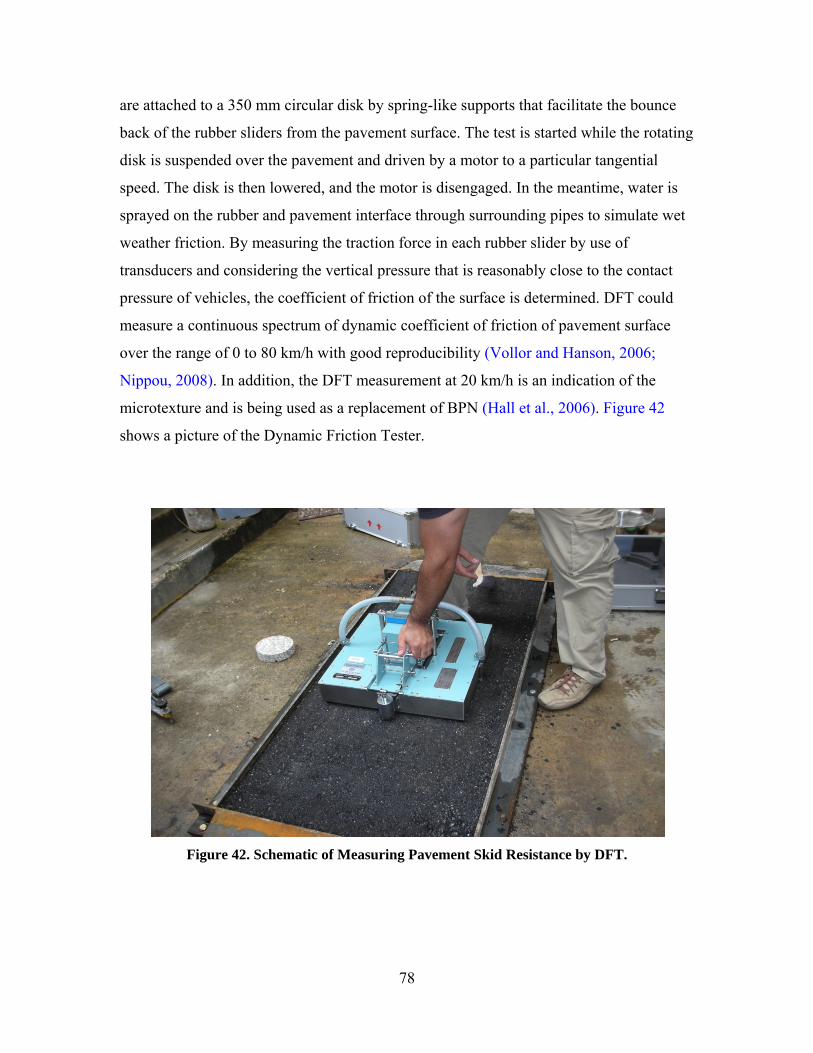
78
are attached to a 350 mm circular disk by spring-like supports that facilitate the bounce
back of the rubber sliders from the pavement surface. The test is started while the rotating
disk is suspended over the pavement and driven by a motor to a particular tangential
speed. The disk is then lowered, and the motor is disengaged. In the meantime, water is
sprayed on the rubber and pavement interface through surrounding pipes to simulate wet
weather friction. By measuring the traction force in each rubber slider by use of
transducers and considering the vertical pressure that is reasonably close to the contact
pressure of vehicles, the coefficient of friction of the surface is determined. DFT could
measure a continuous spectrum of dynamic coefficient of friction of pavement surface
over the range of 0 to 80 km/h with good reproducibility (Vollor and Hanson, 2006;
Nippou, 2008). In addition, the DFT measurement at 20 km/h is an indication of the
microtexture and is being used as a replacement of BPN (Hall et al., 2006). Figure 42
shows a picture of the Dynamic Friction Tester.
Figure 42. Schematic of Measuring Pavement Skid Resistance by DFT.

79
Circular Texture Meter
The most current technology in measuring pavement macrotexture is the Circular
Texture Meter described in ASTM E2157. In this device, a Charged Couple Device
(CCD) laser displacement sensor mounted on an arm 80 mm above the surface rotates
around in a circle with a 142 mm radius. A motor at a tangential velocity of 6 mm/min
drives the arm. The CCD laser takes 1024 samples of the pavement surface in one round
with 0.87 mm spacing. The data are converted to digital format and stored in the memory
of a laptop. To calculate the Mean Pavement Depth, the data are divided into eight equal
111.5 mm arcs. The calculated MPD for each segment is averaged and presented as MPD
for the test surface. The individual MPD values for each segment are also available for
further investigation (tics, 2008). Figure 43 shows a picture of a CTMeter.
Figure 43. CTMeter (Courtesy of Hanson and Prowell, 2004).
EXPERIMENTAL SETUP
Thirteen different slabs were prepared and polished by the polishing machine. The
measurements were done after predefined polishing cycles. The polishing cycles

80
continued to 100,000 cycles for dense mixes and 200,000 cycles for PFC mixtures.
Table 8 presents the different slabs and polishing cycles for designed mixtures.
Table 8. Experimental Setup
Mixture Type Aggregate Type Polishing Cycles
Type C
Beckman
Before Polishing, 5000, 10,000,
20,000, 35,000, 50,000, 75,000,
100,000 cycles, Completely Polished
Brownwood
Brownlee
El Paso
Fordyce
50% Beckman + 50% Brownlee
PFC
Beckman Before Polishing, 5000, 10,000,
20,000, 35,000, 50,000, 75,000,
100,000, 150,000, 200,000 cycles,
Completely Polished
Brownwood
Brownlee
El Paso
Type D Beckman Before Polishing, 5000, 10,000,
20,000, 35,000, 50,000, 75,000,
100,000 cycles, Completely Polished
Brownlee
50% Beckman + 50% Brownlee
According to Table 8, each slab was prepared and tested the day after compaction.
The sand patch test, British pendulum test, DFT, and CTMeter were conducted on the
slabs before the slab was subjected to any polishing. Then, the polisher was placed on top
of the slab and the polishing started.
All Type D mixes degraded after 5000 polishing cycles and showed signs of
raveling (Figure 44). Due to raveling occurring in these mixes, researchers decided to
discontinue polishing these mixes, and they were dropped from the experimental design
program.
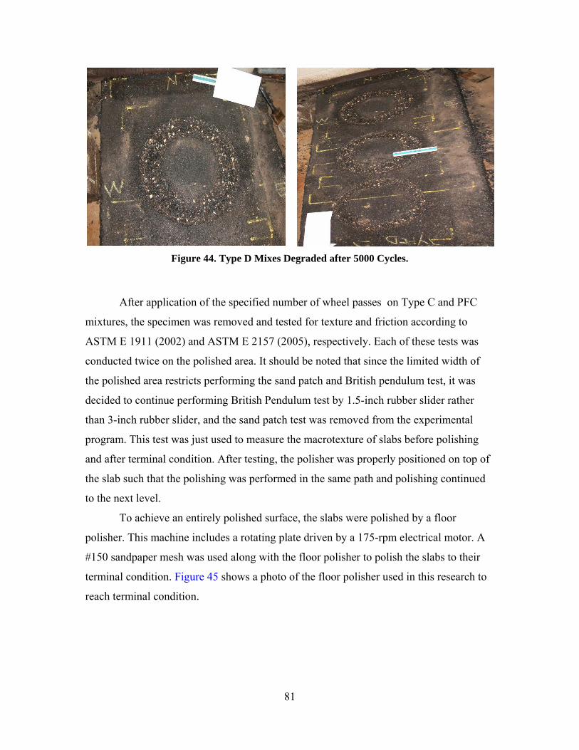
81
Figure 44. Type D Mixes Degraded after 5000 Cycles.
After application of the specified number of wheel passes on Type C and PFC
mixtures, the specimen was removed and tested for texture and friction according to
ASTM E 1911 (2002) and ASTM E 2157 (2005), respectively. Each of these tests was
conducted twice on the polished area. It should be noted that since the limited width of
the polished area restricts performing the sand patch and British pendulum test, it was
decided to continue performing British Pendulum test by 1.5-inch rubber slider rather
than 3-inch rubber slider, and the sand patch test was removed from the experimental
program. This test was just used to measure the macrotexture of slabs before polishing
and after terminal condition. After testing, the polisher was properly positioned on top of
the slab such that the polishing was performed in the same path and polishing continued
to the next level.
To achieve an entirely polished surface, the slabs were polished by a floor
polisher. This machine includes a rotating plate driven by a 175-rpm electrical motor. A
#150 sandpaper mesh was used along with the floor polisher to polish the slabs to their
terminal condition. Figure 45 shows a photo of the floor polisher used in this research to
reach terminal condition.

82
Figure 45. Floor Polisher.
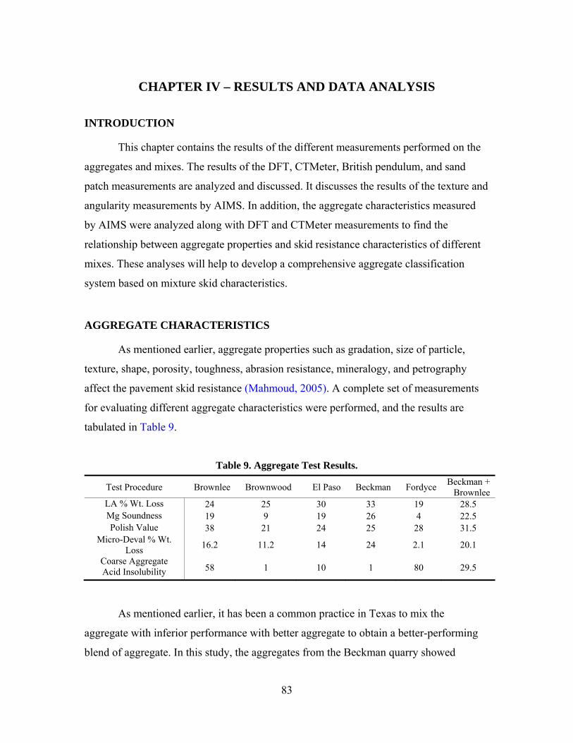
83
CHAPTER IV – RESULTS AND DATA ANALYSIS
INTRODUCTION
This chapter contains the results of the different measurements performed on the
aggregates and mixes. The results of the DFT, CTMeter, British pendulum, and sand
patch measurements are analyzed and discussed. It discusses the results of the texture and
angularity measurements by AIMS. In addition, the aggregate characteristics measured
by AIMS were analyzed along with DFT and CTMeter measurements to find the
relationship between aggregate properties and skid resistance characteristics of different
mixes. These analyses will help to develop a comprehensive aggregate classification
system based on mixture skid characteristics.
AGGREGATE CHARACTERISTICS
As mentioned earlier, aggregate properties such as gradation, size of particle,
texture, shape, porosity, toughness, abrasion resistance, mineralogy, and petrography
affect the pavement skid resistance (Mahmoud, 2005). A complete set of measurements
for evaluating different aggregate characteristics were performed, and the results are
tabulated in Table 9.
Table 9. Aggregate Test Results.
Test Procedure Brownlee Brownwood El Paso Beckman Fordyce Beckman + Brownlee
LA % Wt. Loss 24 25 30 33 19 28.5 Mg Soundness 19 9 19 26 4 22.5 Polish Value 38 21 24 25 28 31.5
Micro-Deval % Wt. Loss 16.2 11.2 14 24 2.1 20.1
Coarse Aggregate Acid Insolubility 58 1 10 1 80 29.5
As mentioned earlier, it has been a common practice in Texas to mix the
aggregate with inferior performance with better aggregate to obtain a better-performing
blend of aggregate. In this study, the aggregates from the Beckman quarry showed
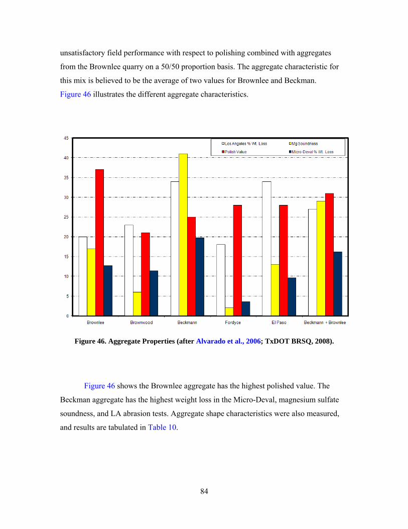
84
unsatisfactory field performance with respect to polishing combined with aggregates
from the Brownlee quarry on a 50/50 proportion basis. The aggregate characteristic for
this mix is believed to be the average of two values for Brownlee and Beckman.
Figure 46 illustrates the different aggregate characteristics.
Figure 46. Aggregate Properties (after Alvarado et al., 2006; TxDOT BRSQ, 2008).
Figure 46 shows the Brownlee aggregate has the highest polished value. The
Beckman aggregate has the highest weight loss in the Micro-Deval, magnesium sulfate
soundness, and LA abrasion tests. Aggregate shape characteristics were also measured,
and results are tabulated in Table 10.
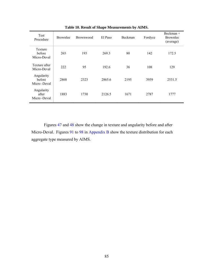
85
Table 10. Result of Shape Measurements by AIMS.
Test Procedure Brownlee Brownwood El Paso Beckman Fordyce
Beckman + Brownlee (average)
Texture before
Micro-Deval 265 193 269.3 80 142 172.5
Texture after Micro-Deval 222 95 192.6 36 108 129
Angularity before
Micro -Deval 2868 2323 2865.6 2195 3959 2531.5
Angularity after
Micro -Deval 1883 1730 2126.5 1671 2787 1777
Figures 47 and 48 show the change in texture and angularity before and after
Micro-Deval. Figures 91 to 98 in Appendix B show the texture distribution for each
aggregate type measured by AIMS.
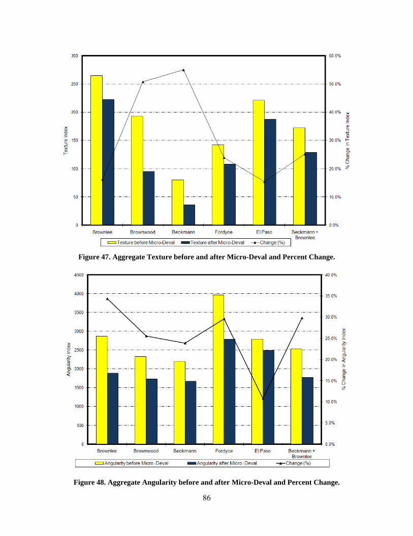
86
Figure 47. Aggregate Texture before and after Micro-Deval and Percent Change.
Figure 48. Aggregate Angularity before and after Micro-Deval and Percent Change.
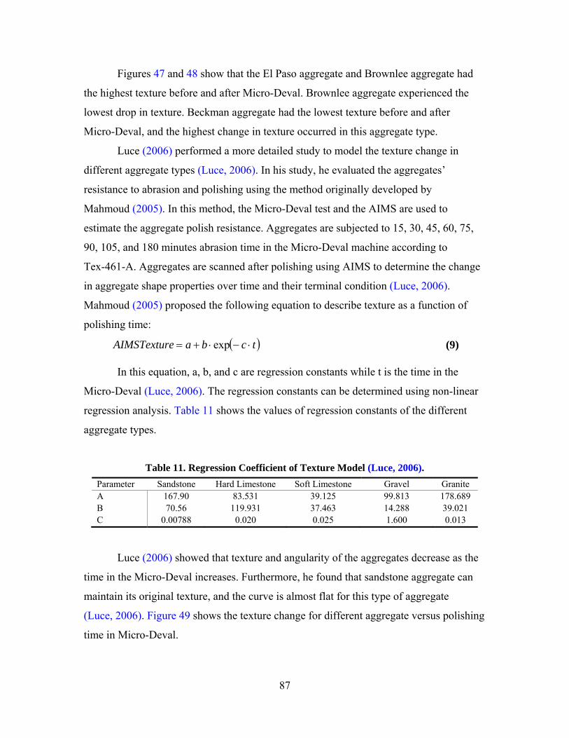
87
Figures 47 and 48 show that the El Paso aggregate and Brownlee aggregate had
the highest texture before and after Micro-Deval. Brownlee aggregate experienced the
lowest drop in texture. Beckman aggregate had the lowest texture before and after
Micro-Deval, and the highest change in texture occurred in this aggregate type.
Luce (2006) performed a more detailed study to model the texture change in
different aggregate types (Luce, 2006). In his study, he evaluated the aggregates’
resistance to abrasion and polishing using the method originally developed by
Mahmoud (2005). In this method, the Micro-Deval test and the AIMS are used to
estimate the aggregate polish resistance. Aggregates are subjected to 15, 30, 45, 60, 75,
90, 105, and 180 minutes abrasion time in the Micro-Deval machine according to
Tex-461-A. Aggregates are scanned after polishing using AIMS to determine the change
in aggregate shape properties over time and their terminal condition (Luce, 2006).
Mahmoud (2005) proposed the following equation to describe texture as a function of
polishing time:
( )tcbaTextureAIMS ⋅−⋅+= exp (9)
In this equation, a, b, and c are regression constants while t is the time in the
Micro-Deval (Luce, 2006). The regression constants can be determined using non-linear
regression analysis. Table 11 shows the values of regression constants of the different
aggregate types.
Table 11. Regression Coefficient of Texture Model (Luce, 2006). Parameter Sandstone Hard Limestone Soft Limestone Gravel Granite A 167.90 83.531 39.125 99.813 178.689 B 70.56 119.931 37.463 14.288 39.021 C 0.00788 0.020 0.025 1.600 0.013
Luce (2006) showed that texture and angularity of the aggregates decrease as the
time in the Micro-Deval increases. Furthermore, he found that sandstone aggregate can
maintain its original texture, and the curve is almost flat for this type of aggregate
(Luce, 2006). Figure 49 shows the texture change for different aggregate versus polishing
time in Micro-Deval.
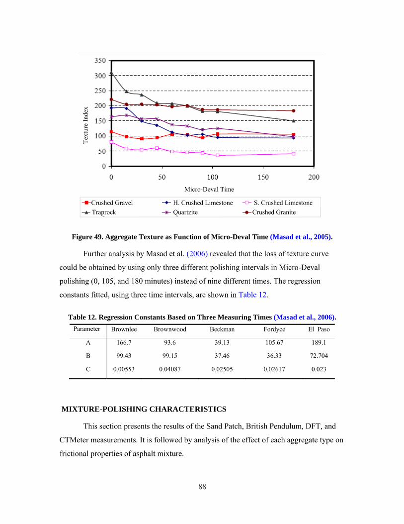
88
Figure 49. Aggregate Texture as Function of Micro-Deval Time (Masad et al., 2005).
Further analysis by Masad et al. (2006) revealed that the loss of texture curve
could be obtained by using only three different polishing intervals in Micro-Deval
polishing (0, 105, and 180 minutes) instead of nine different times. The regression
constants fitted, using three time intervals, are shown in Table 12.
Table 12. Regression Constants Based on Three Measuring Times (Masad et al., 2006).
Parameter Brownlee Brownwood Beckman Fordyce El Paso
A 166.7 93.6 39.13 105.67 189.1
B 99.43 99.15 37.46 36.33 72.704
C 0.00553 0.04087 0.02505 0.02617 0.023
MIXTURE-POLISHING CHARACTERISTICS
This section presents the results of the Sand Patch, British Pendulum, DFT, and
CTMeter measurements. It is followed by analysis of the effect of each aggregate type on
frictional properties of asphalt mixture.
Crushed Gravel Traprock
H. Crushed Limestone Quartzite
S. Crushed Limestone Crushed Granite
Text
ure
Inde
x
Micro-Deval Time
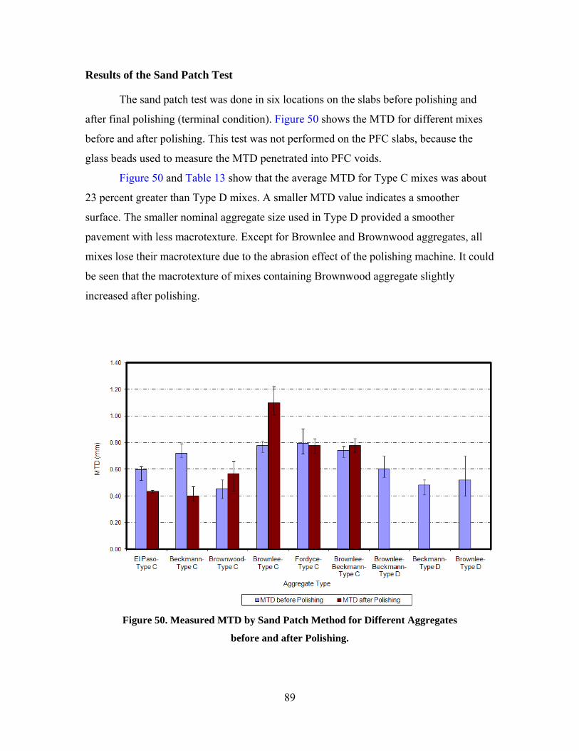
89
Results of the Sand Patch Test
The sand patch test was done in six locations on the slabs before polishing and
after final polishing (terminal condition). Figure 50 shows the MTD for different mixes
before and after polishing. This test was not performed on the PFC slabs, because the
glass beads used to measure the MTD penetrated into PFC voids.
Figure 50 and Table 13 show that the average MTD for Type C mixes was about
23 percent greater than Type D mixes. A smaller MTD value indicates a smoother
surface. The smaller nominal aggregate size used in Type D provided a smoother
pavement with less macrotexture. Except for Brownlee and Brownwood aggregates, all
mixes lose their macrotexture due to the abrasion effect of the polishing machine. It could
be seen that the macrotexture of mixes containing Brownwood aggregate slightly
increased after polishing.
Figure 50. Measured MTD by Sand Patch Method for Different Aggregates
before and after Polishing.
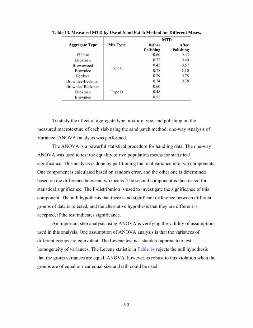
90
Table 13. Measured MTD by Use of Sand Patch Method for Different Mixes.
Aggregate Type Mix Type MTD
Before Polishing
After Polishing
El Paso
Type C
0.60 0.43 Beckman 0.72 0.40
Brownwood 0.45 0.57 Brownlee 0.78 1.10 Fordyce 0.79 0.78
Brownlee-Beckman 0.74 0.78 Brownlee-Beckman
Type D 0.60
Beckman 0.48 Brownlee 0.52
To study the effect of aggregate type, mixture type, and polishing on the
measured macrotexture of each slab using the sand patch method, one-way Analysis of
Variance (ANOVA) analysis was performed.
The ANOVA is a powerful statistical procedure for handling data. The one-way
ANOVA was used to test the equality of two population means for statistical
significance. This analysis is done by partitioning the total variance into two components.
One component is calculated based on random error, and the other one is determined
based on the difference between two means. The second component is then tested for
statistical significance. The F-distribution is used to investigate the significance of this
component. The null hypothesis that there is no significant difference between different
groups of data is rejected, and the alternative hypothesis that they are different is
accepted, if the test indicates significance.
An important step analysis using ANOVA is verifying the validity of assumptions
used in this analysis. One assumption of ANOVA analysis is that the variances of
different groups are equivalent. The Levene test is a standard approach to test
homogeneity of variances. The Levene statistic in Table 14 rejects the null hypothesis
that the group variances are equal. ANOVA, however, is robust to this violation when the
groups are of equal or near equal size and still could be used.
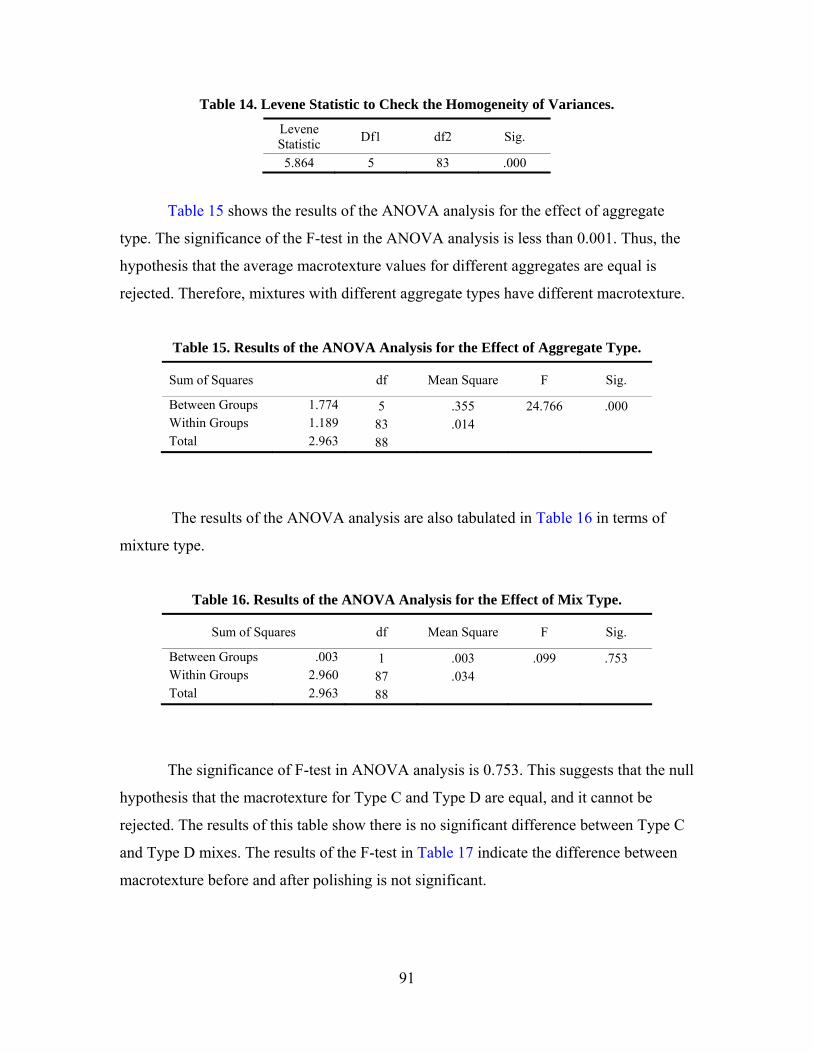
91
Table 14. Levene Statistic to Check the Homogeneity of Variances.
Levene Statistic Df1 df2 Sig.
5.864 5 83 .000
Table 15 shows the results of the ANOVA analysis for the effect of aggregate
type. The significance of the F-test in the ANOVA analysis is less than 0.001. Thus, the
hypothesis that the average macrotexture values for different aggregates are equal is
rejected. Therefore, mixtures with different aggregate types have different macrotexture.
Table 15. Results of the ANOVA Analysis for the Effect of Aggregate Type.
Sum of Squares df Mean Square F Sig.
Between Groups 1.774 5 .355 24.766 .000 Within Groups 1.189 83 .014 Total 2.963 88
The results of the ANOVA analysis are also tabulated in Table 16 in terms of
mixture type.
Table 16. Results of the ANOVA Analysis for the Effect of Mix Type.
Sum of Squares df Mean Square F Sig.
Between Groups .003 1 .003 .099 .753 Within Groups 2.960 87 .034 Total 2.963 88
The significance of F-test in ANOVA analysis is 0.753. This suggests that the null
hypothesis that the macrotexture for Type C and Type D are equal, and it cannot be
rejected. The results of this table show there is no significant difference between Type C
and Type D mixes. The results of the F-test in Table 17 indicate the difference between
macrotexture before and after polishing is not significant.
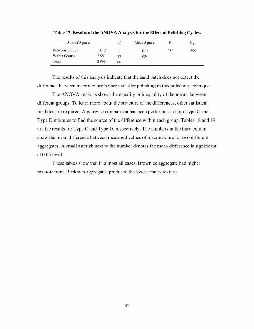
92
Table 17. Results of the ANOVA Analysis for the Effect of Polishing Cycles.
Sum of Squares df Mean Square F Sig.
Between Groups .012 1 .012 .350 .555 Within Groups 2.951 87 .034 Total 2.963 88
The results of this analysis indicate that the sand patch does not detect the
difference between macrotexture before and after polishing in this polishing technique.
The ANOVA analysis shows the equality or inequality of the means between
different groups. To learn more about the structure of the differences, other statistical
methods are required. A pairwise comparison has been performed in both Type C and
Type D mixtures to find the source of the difference within each group. Tables 18 and 19
are the results for Type C and Type D, respectively. The numbers in the third column
show the mean difference between measured values of macrotexture for two different
aggregates. A small asterisk next to the number denotes the mean difference is significant
at 0.05 level.
These tables show that in almost all cases, Brownlee aggregate had higher
macrotexture. Beckman aggregates produced the lowest macrotexture.
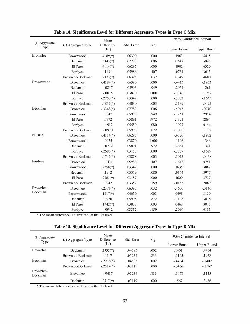
93
Table 18. Significance Level for Different Aggregate Types in Type C Mix.
(I) Aggregate Type (J) Aggregate Type
Mean Difference
(I-J) Std. Error Sig.
95% Confidence Interval
Lower Bound Upper Bound
Brownlee Brownwood .4189(*) .06390 .000 .1963 .6415 Beckman .3343(*) .07783 .006 .0740 .5945 El Paso .4114(*) .06295 .000 .1902 .6326 Fordyce .1431 .05986 .407 -.0751 .3613 Brownlee-Beckman .2373(*) .06395 .032 .0146 .4600 Brownwood Brownlee -.4189(*) .06390 .000 -.6415 -.1963 Beckman -.0847 .05993 .949 -.2954 .1261 El Paso -.0075 .03870 1.000 -.1346 .1196 Fordyce -.2758(*) .03342 .000 -.3882 -.1635 Brownlee-Beckman -.1817(*) .04030 .003 -.3139 -.0495 Beckman Brownlee -.3343(*) .07783 .006 -.5945 -.0740 Brownwood .0847 .05993 .949 -.1261 .2954 El Paso .0772 .05891 .972 -.1321 .2864 Fordyce -.1912 .05559 .080 -.3977 .0154 Brownlee-Beckman -.0970 .05998 .872 -.3078 .1138 El Paso Brownlee -.4114(*) .06295 .000 -.6326 -.1902 Brownwood .0075 .03870 1.000 -.1196 .1346 Beckman -.0772 .05891 .972 -.2864 .1321 Fordyce -.2683(*) .03157 .000 -.3737 -.1629 Brownlee-Beckman -.1742(*) .03878 .003 -.3015 -.0468 Fordyce Brownlee -.1431 .05986 .407 -.3613 .0751 Brownwood .2758(*) .03342 .000 .1635 .3882 Beckman .1912 .05559 .080 -.0154 .3977 El Paso .2683(*) .03157 .000 .1629 .3737 Brownlee-Beckman .0942 .03352 .159 -.0185 .2069 Brownlee-Beckman
Brownlee -.2373(*) .06395 .032 -.4600 -.0146 Brownwood .1817(*) .04030 .003 .0495 .3139
Beckman .0970 .05998 .872 -.1138 .3078 El Paso .1742(*) .03878 .003 .0468 .3015 Fordyce -.0942 .03352 .159 -.2069 .0185
* The mean difference is significant at the .05 level.
Table 19. Significance Level for Different Aggregate Types in Type D Mix.
(I) Aggregate Type (J) Aggregate Type
Mean Difference
(I-J) Std. Error Sig.
95% Confidence Interval
Lower Bound Upper Bound Brownlee Beckman .2933(*) .04685 .002 .1402 .4464 Brownlee-Beckman .0417 .05254 .833 -.1145 .1978 Beckman Brownlee -.2933(*) .04685 .002 -.4464 -.1402 Brownlee-Beckman -.2517(*) .03119 .000 -.3466 -.1567 Brownlee-Beckman Brownlee -.0417 .05254 .833 -.1978 .1145
Beckman .2517(*) .03119 .000 .1567 .3466 * The mean difference is significant at the .05 level.
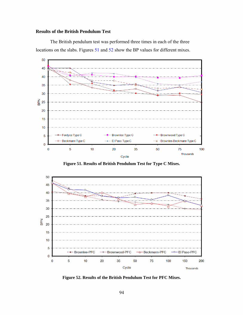
94
Results of the British Pendulum Test
The British pendulum test was performed three times in each of the three
locations on the slabs. Figures 51 and 52 show the BP values for different mixes.
Figure 51. Results of British Pendulum Test for Type C Mixes.
Figure 52. Results of the British Pendulum Test for PFC Mixes.

95
As a general trend, it is clear that the BP value decreases as the number of
polishing cycles increase. The rate of decrease in the British Pendulum Value is
dependent on the aggregate type. Table 20 summarizes the results of the ANOVA
analysis at 95 percent confidence level for different aggregates. The results show that
there is a significant difference between the mean BP values for each aggregate type in
each polishing cycle. Moreover, it indicates the polisher has an effect in decreasing the
surface skid resistance and obviously can polish the surface.
Table 21 shows the significance level of the equality of mean measured BP values
at different numbers of polishing cycles. This table shows that in almost all
cases—except sandstone—the significance is negligible, and this analysis supports the
idea that there is significant difference between measured BP values in different
aggregates at a 95 percent confidence level. Further study in this section, however,
revealed that this difference is only due to Brownlee aggregate, and there is no significant
difference between other aggregates.
Another ANOVA analysis was done to examine the effect of mixture type on
frictional characteristics of asphalt pavement (Table 22). The results indicate that there is
no statistical difference between the skid resistance of Type C and PFC mixes containing
Brownlee aggregate. Furthermore, this aggregate has the same frictional performance in
Type C and PFC mixes in both low and high numbers of polishing cycles. This is a result
of continuous renewal of the aggregate surface exposed to a rubber slider. Moreover,
Brownlee aggregate consists of hard particles in a softer matrix. Wearing the softer
matrix off the aggregate allows the new hard particles to be exposed to traffic and will
help this mix to maintain its frictional properties. The PFC and Type C mixes containing
Brownwood aggregate statistically have equal BP values in low-polishing cycles;
however, when the polishing cycles increase, the PFC could maintain its skid properties
relatively better than Type C mixes, and the BP value is higher. The difference between
the BP value of Type C and PFC mixes containing Beckman aggregate is always
significant. Moreover, PFC mixes containing Beckman aggregate always have a higher
BP value than Type C mixes. The difference between skid properties of the mixes
containing El Paso aggregate does not follow a clear trend. The PFC mixes containing
this kind of aggregate are likely to have higher BP value in low-polishing cycles, and the

96
results of the analysis do not show significant difference between PFC and Type C mixes
in high-polishing cycles.
Table 20. Significance Level for the Effect of Different Polishing Cycles
on Mixtures with Different Aggregates.
Aggregate Type Mix Type Polishing Cycle (thousands)
0 5 10 20 35 50 75 100 150 200 El Paso
Type C 0.039 0.009 0.002 0 0 0 0 0 NA NA
Beckman Brownwood Brownlee Fordyce Brownlee-Beckman Brownlee
PFC 0 0.001 0 0 0.054 0 0 0 0 0 El Paso Brownwood Beckman
Table 21. Significance Level for the Mean BP Values for Different Loading Cycles.
Aggregate Type Mix Type Sig.
El Paso
Type C
0.0001 Beckman 0 Brownwood 0 Brownlee 0.0581 Fordyce 0 Brownlee-Beckman 0 Brownlee
PFC
0 El Paso 0 Brownwood 0 Beckman 0
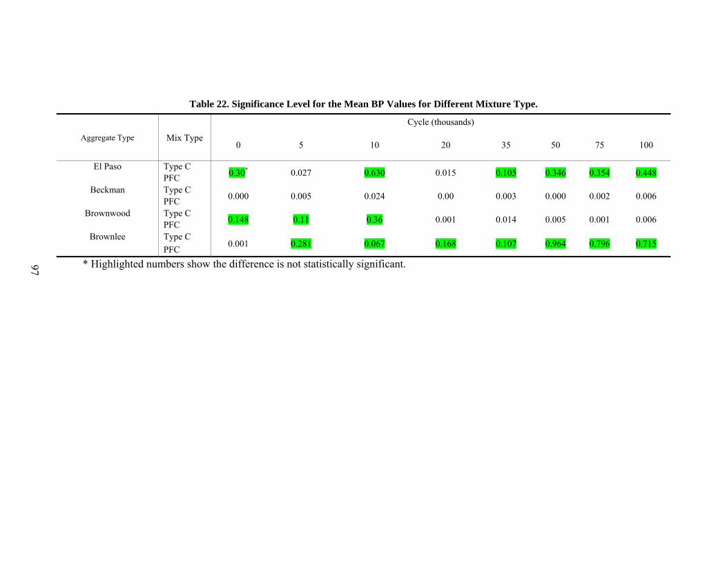
97
Table 22. Significance Level for the Mean BP Values for Different Mixture Type.
Aggregate Type Mix Type
Cycle (thousands)
0 5 10 20 35 50 75 100
El Paso Type C 0.30* 0.027 0.630 0.015 0.105 0.346 0.354 0.448 PFC
Beckman Type C 0.000 0.005 0.024 0.00 0.003 0.000 0.002 0.006 PFC
Brownwood Type C 0.148 0.11 0.36 0.001 0.014 0.005 0.001 0.006 PFC
Brownlee Type C 0.001 0.281 0.067 0.168 0.107 0.964 0.796 0.715 PFC
* Highlighted numbers show the difference is not statistically significant.

98
To have a better understanding of the variation of the BP values for different
mixes, the equation suggested by Mahmoud (2005) was fitted to the data substituting
texture with British Pendulum value and time with polishing cycles in terms of 1000
cycles. This equation has the form of Equation 9.
Figures 53 to 62 show the data and the fitted lines for different mixes. The results
show that this equation could fit the data very well.
Table 23 shows the values of the regression coefficients for different mixes after
removing the outliers and fitting the function by the least square method.
Table 23. Regression Coefficients for Different Aggregate. Aggregate type Mix type A B C
El Paso
Type C
35 9 0.026
Beckman 29 16 0.091
Brownwood 30 16 0.140
Brownlee 39 3 0.027
Fordyce 32 14 0.064
Brownlee-Beckman 33 11 0.053
Brownlee
PFC
37 3 0.052
El Paso 35 11 0.042
Brownwood 32 15 0.070
Beckman 33 11 0.050

99
Figure 53. British Pendulum Values for El Paso Aggregate vs. Polishing Cycles.
Figure 54. British Pendulum Values for Beckman Aggregate vs. Polishing Cycles.
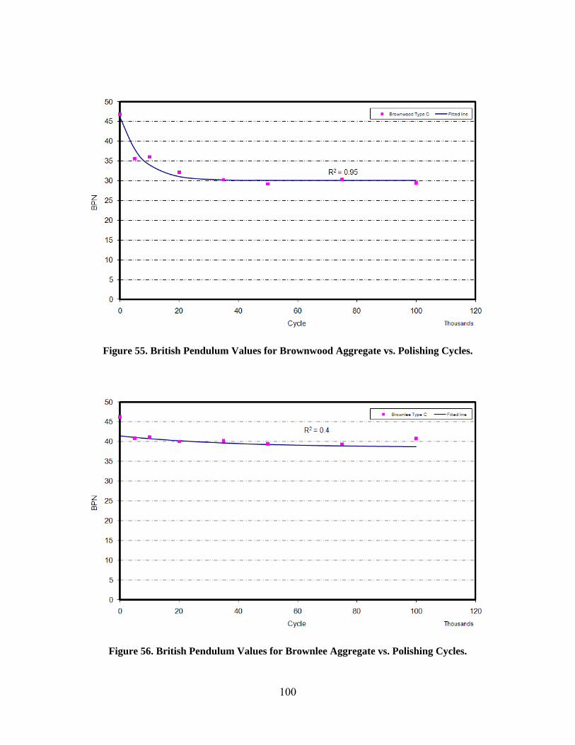
100
Figure 55. British Pendulum Values for Brownwood Aggregate vs. Polishing Cycles.
Figure 56. British Pendulum Values for Brownlee Aggregate vs. Polishing Cycles.
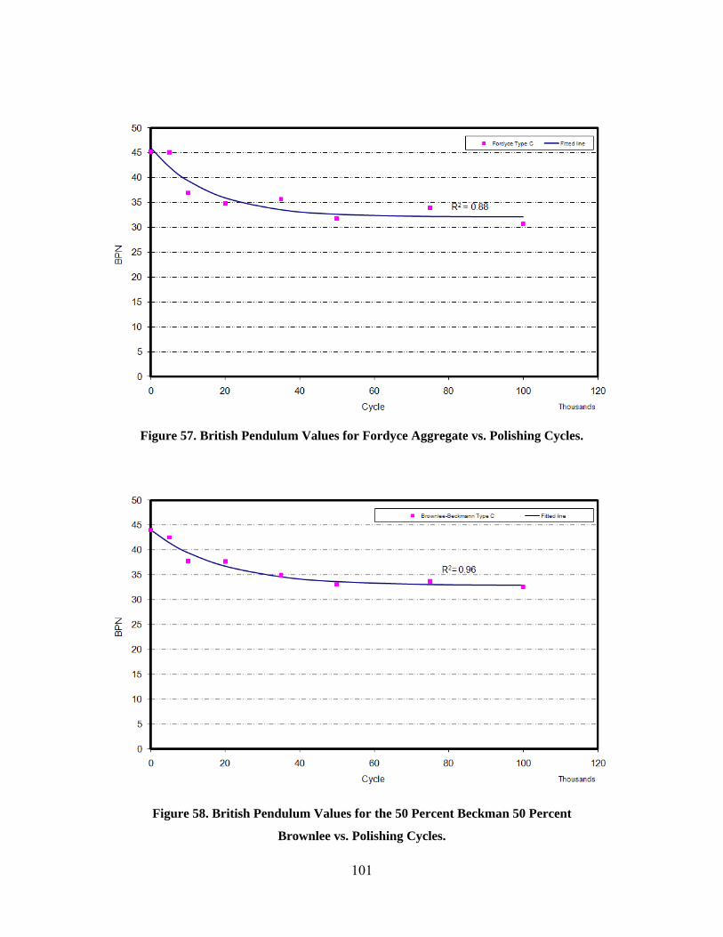
101
Figure 57. British Pendulum Values for Fordyce Aggregate vs. Polishing Cycles.
Figure 58. British Pendulum Values for the 50 Percent Beckman 50 Percent
Brownlee vs. Polishing Cycles.

102
Figure 59. British Pendulum Values for El Paso Aggregate vs. Polishing Cycles in PFC Mix.
Figure 60. British Pendulum Values for Brownlee Aggregate vs. Polishing
Cycles in PFC Mix.

103
Figure 61. British Pendulum Values for Brownwood Aggregate vs. Polishing
Cycles in PFC Mix.
Figure 62. British Pendulum Values for Beckman Aggregate vs. Polishing
Cycles in PFC Mix.

104
Figures 56 and 60 for Brownlee aggregate show that the change of BP values
versus polishing cycle is very small. The same results were reported by Luce (2006). This
aggregate has the lowest change with regard to the polishing cycles, highest terminal
value compared to other aggregates. Moreover, this small change in BP value against
polishing cycles in Brownlee aggregate texture contributes to its high-skid resistance.
El Paso aggregate has the second-lowest rate of decrease in BP value against polishing
cycles and is polish-resistant. Mixing Beckman aggregate with Brownlee aggregate
shows promising results since this mixture has the third-lowest rate of change versus
polishing cycle. Brownwood aggregate has the highest rate of BP value lost versus
polishing cycle and does not have a high terminal BP value. BP values for Brownlee
aggregate in the PFC mixture are almost constant, which is similar to Type C mixes.
The results of the ANOVA analysis tabulated in Table 24 show the comparison
between measured BP values for each pair of aggregates. In this table, the numbers in the
third column show the mean difference between BP values of corresponding aggregates.
An asterisk next to a number shows the difference is significant at the 0.05 level.
Table 24 does not show a statistical difference between each pair except for very high
values (i.e., Brownlee aggregate) and other aggregates. This indicates the limitation of
British Pendulum to detect the difference between frictional performances of aggregates
with known differences in frictional characteristics.
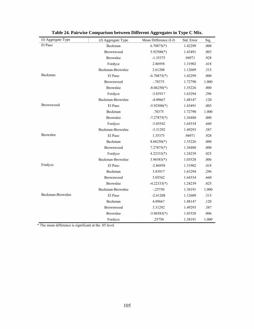
105
Table 24. Pairwise Comparison between Different Aggregates in Type C Mix. (I) Aggregate Type (J) Aggregate Type Mean Difference (I-J) Std. Error Sig. El Paso Beckman 6.70875(*) 1.42299 .000 Brownwood 5.92500(*) 1.43491 .003 Brownlee -1.35375 .94971 .928 Fordyce 2.86958 1.31902 .418 Beckman-Brownlee 2.61208 1.12609 .315 Beckman El Paso -6.70875(*) 1.42299 .000 Brownwood -.78375 1.72790 1.000 Brownlee -8.06250(*) 1.35226 .000 Fordyce -3.83917 1.63294 .296 Beckman-Brownlee -4.09667 1.48147 .120 Brownwood El Paso -5.92500(*) 1.43491 .003 Beckman .78375 1.72790 1.000 Brownlee -7.27875(*) 1.36480 .000 Fordyce -3.05542 1.64334 .660 Beckman-Brownlee -3.31292 1.49293 .387 Brownlee El Paso 1.35375 .94971 .928 Beckman 8.06250(*) 1.35226 .000 Brownwood 7.27875(*) 1.36480 .000 Fordyce 4.22333(*) 1.24239 .025 Beckman-Brownlee 3.96583(*) 1.03528 .006 Fordyce El Paso -2.86958 1.31902 .418 Beckman 3.83917 1.63294 .296 Brownwood 3.05542 1.64334 .660 Brownlee -4.22333(*) 1.24239 .025 Beckman-Brownlee -.25750 1.38191 1.000 Beckman-Brownlee El Paso -2.61208 1.12609 .315 Beckman 4.09667 1.48147 .120 Brownwood 3.31292 1.49293 .387 Brownlee -3.96583(*) 1.03528 .006 Fordyce .25750 1.38191 1.000
* The mean difference is significant at the .05 level.
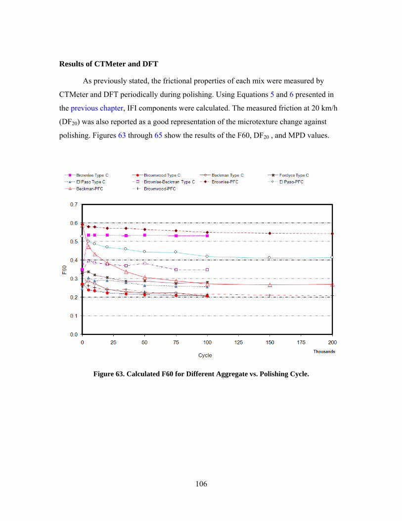
106
Results of CTMeter and DFT
As previously stated, the frictional properties of each mix were measured by
CTMeter and DFT periodically during polishing. Using Equations 5 and 6 presented in
the previous chapter, IFI components were calculated. The measured friction at 20 km/h
(DF20) was also reported as a good representation of the microtexture change against
polishing. Figures 63 through 65 show the results of the F60, DF20 , and MPD values.
Figure 63. Calculated F60 for Different Aggregate vs. Polishing Cycle.

107
Figure 64. Coefficient of Friction for Different Aggregate vs. Polishing Cycle at 20 km/h.
Figure 65. MPD for Different Aggregate vs. Polishing Cycle.

108
It is evident from Figure 64 that the coefficient of friction decreases when the
polishing cycle increases. In addition, some aggregates such as Beckman aggregate show
a rapid change in their measured coefficient of friction, and some of them such as
Brownlee aggregate remain almost constant during the polishing. It is clear that after a
particular number of polishing cycles, each mix reached a terminal condition in which no
other changes occur afterwards. The rate of change and the terminal value of DF20 can be
an indication of an aggregate susceptibility to polishing and will be investigated in this
report.
The MPD values of different mixes in Figure 65 vary in terms of polishing cycles
and do not show a clear trend. Moreover, small changes in MPD could be related to
aggregate abrasion during polishing or experimental error. For some types of aggregate
(Brownlee aggregate), aggregate raveling due to moisture susceptibility was also noticed.
Figure 63 shows the calculated F60 based on the Equations 5 and 6. The F60
decreases as the polishing cycles increase. Moreover, the variation of microtexture—
DF20—has a more important role on the variation of F60 than macrotexture does.
Therefore, the variation of DF20 and F60 are consistent and following the same trend.
ANOVA analysis was performed to study the effect of polishing cycles, speed, and
aggregate type on measured values of DF20 for different mixes in different speed and
polishing cycles. The results are tabulated in Tables 25 and 26.

109
Table 25. Significance Level (p-value) of the Mean DF20 Values for Different Aggregate Types in Type C Mix.
Mix Type Aggregate Speed Polishing Before Polish 5000 10,000 20,000
Speed Effect
Aggregate Type
Speed Effect
Aggregate Type
Speed Effect
Aggregate Type
Speed Effect
Aggregate Type
Type C
Brownlee-Beckman 20 0.00 0.00 0.00 0.00 0.00 0.00 0.00 0.00 0.00 40 0.00 0.00 0.00 0.00 0.00 60 0.00 0.00 0.00 0.00 0.00 80 0.00 0.00 0.00 0.00 0.00
El Paso 20 0.00 0.00 0.00 0.00 0.00 0.00 0.00 0.00 0.00 40 0.00 0.00 0.00 0.00 0.00 60 0.00 0.00 0.00 0.00 0.00 80 0.00 0.00 0.00 0.00 0.00
Fordyce 20 0.00 0.00 0.00 0.00 0.00 0.00 0.00 0.00 0.00 40 0.00 0.00 0.00 0.00 0.00 60 0.00 0.00 0.00 0.00 0.00 80 0.00 0.00 0.00 0.00 0.00
Brownwood 20 0.00 0.00 0.00 0.00 0.00 0.00 0.00 0.00 0.00 40 0.00 0.00 0.00 0.00 0.00 60 0.00 0.00 0.00 0.00 0.00 80 0.00 0.00 0.00 0.00 0.00
Brownlee 20 0.00 0.00 0.00 0.00 0.00 0.00 0.00 0.00 0.00 40 0.00 0.00 0.00 0.00 0.00 60 0.00 0.00 0.00 0.00 0.00 80 0.00 0.00 0.00 0.00 0.00
Beckman 20 0.00 0.00 0.00 0.00 0.00 0.00 0.00 0.00 0.00 40 0.00 0.00 0.00 0.00 0.00 60 0.00 0.00 0.00 0.00 0.00 80 0.00 0.00 0.00 0.00 0.00
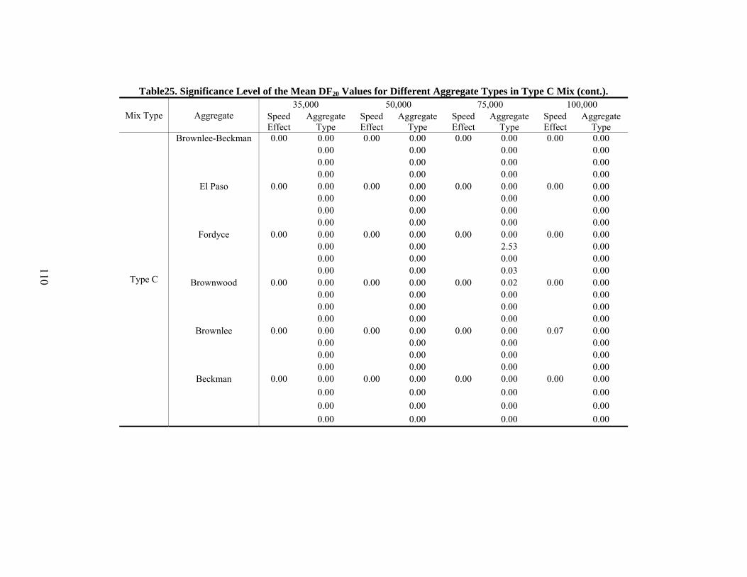
110
Table25. Significance Level of the Mean DF20 Values for Different Aggregate Types in Type C Mix (cont.).
Mix Type Aggregate 35,000 50,000 75,000 100,000
Speed Effect
Aggregate Type
Speed Effect
Aggregate Type
Speed Effect
Aggregate Type
Speed Effect
Aggregate Type
Type C
Brownlee-Beckman 0.00 0.00 0.00 0.00 0.00 0.00 0.00 0.00 0.00 0.00 0.00 0.00 0.00 0.00 0.00 0.00 0.00 0.00 0.00 0.00
El Paso 0.00 0.00 0.00 0.00 0.00 0.00 0.00 0.00 0.00 0.00 0.00 0.00 0.00 0.00 0.00 0.00 0.00 0.00 0.00 0.00
Fordyce 0.00 0.00 0.00 0.00 0.00 0.00 0.00 0.00 0.00 0.00 2.53 0.00 0.00 0.00 0.00 0.00 0.00 0.00 0.03 0.00
Brownwood 0.00 0.00 0.00 0.00 0.00 0.02 0.00 0.00 0.00 0.00 0.00 0.00 0.00 0.00 0.00 0.00 0.00 0.00 0.00 0.00
Brownlee 0.00 0.00 0.00 0.00 0.00 0.00 0.07 0.00 0.00 0.00 0.00 0.00 0.00 0.00 0.00 0.00 0.00 0.00 0.00 0.00
Beckman 0.00 0.00 0.00 0.00 0.00 0.00 0.00 0.00 0.00 0.00 0.00 0.00 0.00 0.00 0.00 0.00 0.00 0.00 0.00 0.00

111
Table 26. Significance Level of the Mean DF20 Values for Different Aggregate Types in PFC Mix.
Mix Type Aggregate Speed Polishing Before Polish 5000 10,000 20,000
Speed Effect
Aggregate Type
Speed Effect
Aggregate Type
Speed Effect
Aggregate Type
Speed Effect
Aggregate Type
PFC
El Paso 20 0.00 0.00 0.00 0.00 0.00 0.00 0.00 0.00 0.00 40 0.00 0.00 0.00 0.00 0.00 60 0.00 0.00 0.00 0.00 0.00 80 0.00 0.00 0.00 0.00 0.00
Brownwood 20 0.00 0.00 0.00 0.00 0.00 0.00 0.00 0.11 0.00 40 0.00 0.00 0.00 0.00 0.00 60 0.00 0.00 0.00 0.00 0.00 80 0.00 0.00 0.00 0.00 0.00
Brownlee 20 0.20* 0.00 0.00 0.03 0.00 0.00 0.00 0.09 0.00 40 0.29 0.00 0.00 0.00 0.00 60 0.29 0.00 0.00 0.00 0.00 80 0.38 0.00 0.00 0.00 0.00
Beckman 20 0.00 0.00 0.00 0.00 0.00 0.00 0.00 0.00 0.00 40 0.00 0.00 0.00 0.00 0.00 60 0.00 0.00 0.00 0.00 0.00 80 0.00 0.00 0.00 0.00 0.00
* Highlighted numbers show the difference is not statistically significant.
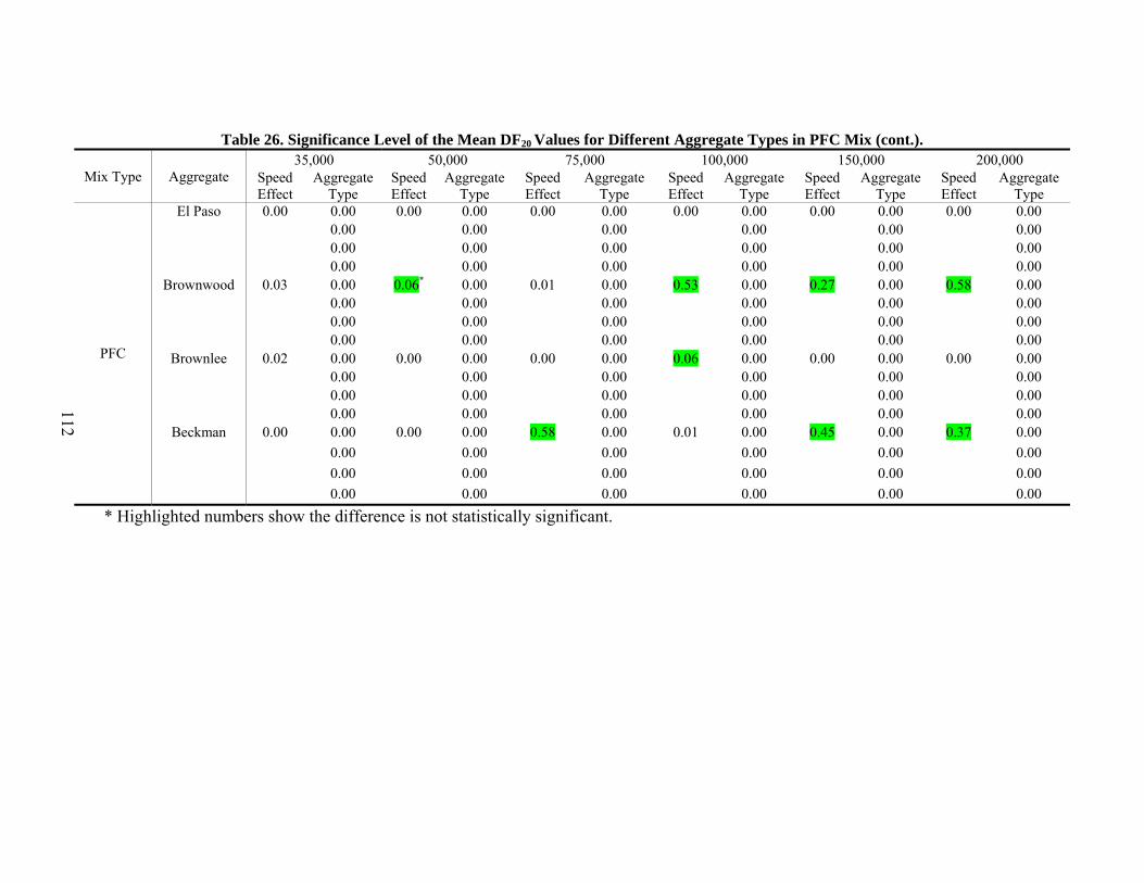
112
Table 26. Significance Level of the Mean DF20 Values for Different Aggregate Types in PFC Mix (cont.).
Mix Type Aggregate 35,000 50,000 75,000 100,000 150,000 200,000
Speed Effect
Aggregate Type
Speed Effect
Aggregate Type
Speed Effect
Aggregate Type
Speed Effect
Aggregate Type
Speed Effect
Aggregate Type
Speed Effect
Aggregate Type
PFC
El Paso 0.00 0.00 0.00 0.00 0.00 0.00 0.00 0.00 0.00 0.00 0.00 0.00 0.00 0.00 0.00 0.00 0.00 0.00 0.00 0.00 0.00 0.00 0.00 0.00 0.00 0.00 0.00 0.00 0.00 0.00
Brownwood 0.03 0.00 0.06* 0.00 0.01 0.00 0.53 0.00 0.27 0.00 0.58 0.00 0.00 0.00 0.00 0.00 0.00 0.00 0.00 0.00 0.00 0.00 0.00 0.00 0.00 0.00 0.00 0.00 0.00 0.00
Brownlee 0.02 0.00 0.00 0.00 0.00 0.00 0.06 0.00 0.00 0.00 0.00 0.00 0.00 0.00 0.00 0.00 0.00 0.00 0.00 0.00 0.00 0.00 0.00 0.00 0.00 0.00 0.00 0.00 0.00 0.00
Beckman 0.00 0.00 0.00 0.00 0.58 0.00 0.01 0.00 0.45 0.00 0.37 0.00 0.00 0.00 0.00 0.00 0.00 0.00 0.00 0.00 0.00 0.00 0.00 0.00 0.00 0.00 0.00 0.00 0.00 0.00
* Highlighted numbers show the difference is not statistically significant.
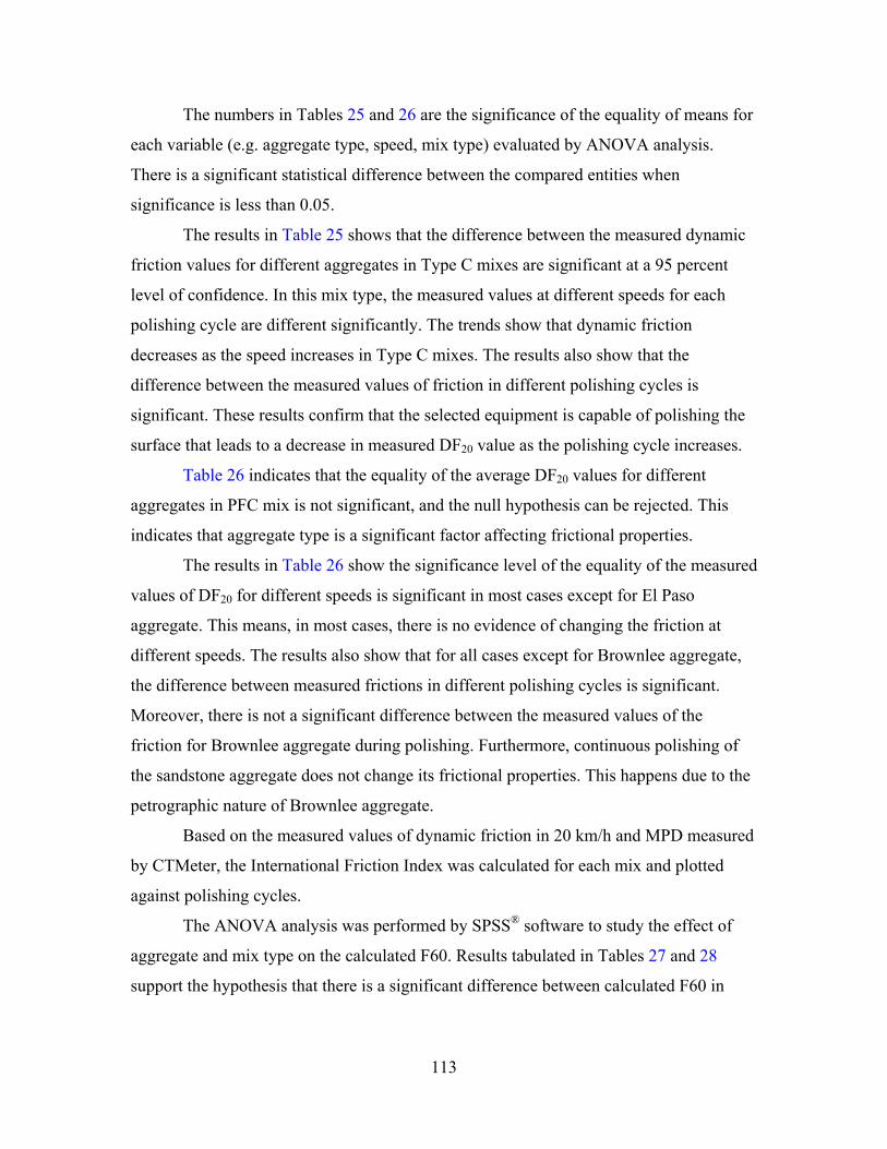
113
The numbers in Tables 25 and 26 are the significance of the equality of means for
each variable (e.g. aggregate type, speed, mix type) evaluated by ANOVA analysis.
There is a significant statistical difference between the compared entities when
significance is less than 0.05.
The results in Table 25 shows that the difference between the measured dynamic
friction values for different aggregates in Type C mixes are significant at a 95 percent
level of confidence. In this mix type, the measured values at different speeds for each
polishing cycle are different significantly. The trends show that dynamic friction
decreases as the speed increases in Type C mixes. The results also show that the
difference between the measured values of friction in different polishing cycles is
significant. These results confirm that the selected equipment is capable of polishing the
surface that leads to a decrease in measured DF20 value as the polishing cycle increases.
Table 26 indicates that the equality of the average DF20 values for different
aggregates in PFC mix is not significant, and the null hypothesis can be rejected. This
indicates that aggregate type is a significant factor affecting frictional properties.
The results in Table 26 show the significance level of the equality of the measured
values of DF20 for different speeds is significant in most cases except for El Paso
aggregate. This means, in most cases, there is no evidence of changing the friction at
different speeds. The results also show that for all cases except for Brownlee aggregate,
the difference between measured frictions in different polishing cycles is significant.
Moreover, there is not a significant difference between the measured values of the
friction for Brownlee aggregate during polishing. Furthermore, continuous polishing of
the sandstone aggregate does not change its frictional properties. This happens due to the
petrographic nature of Brownlee aggregate.
Based on the measured values of dynamic friction in 20 km/h and MPD measured
by CTMeter, the International Friction Index was calculated for each mix and plotted
against polishing cycles.
The ANOVA analysis was performed by SPSS® software to study the effect of
aggregate and mix type on the calculated F60. Results tabulated in Tables 27 and 28
support the hypothesis that there is a significant difference between calculated F60 in

114
Type C and PFC mixes. This result indicates that the PFC mixture has higher F60 value
and consequently can provide better skid resistance.
Table 27. Results of Comparing Calculated Values F60 for Type C and PFC Mixes.
Mix Type N Mean Std. Deviation Std. Error
Mean Type C 132 .3190 .09861 .00858 PFC 105 .4058 .13285 .01296
Table 28. Results of the T-test for Comparing F60 Mean Values in Type C and PFC Mixes.
T-Value
df
Sig. (2-Tailed)
Mean Difference
Std. Error Difference
95% Confidence Interval of the
Difference Lower Upper
-5.581 186.669 .000 -.0868 .01555 -.11745 -.05610
An equation with the same form as the one proposed by Mahmoud (2005)
(Equation 9) was fitted to the data. Figures 66 through 69 show the measured DF20 and
F60 values and the fitted curves for different mixes. The results show that this equation
could fit the data substituting texture with F60 or DF20 values and time with polishing
cycles in terms of 1000 cycles.
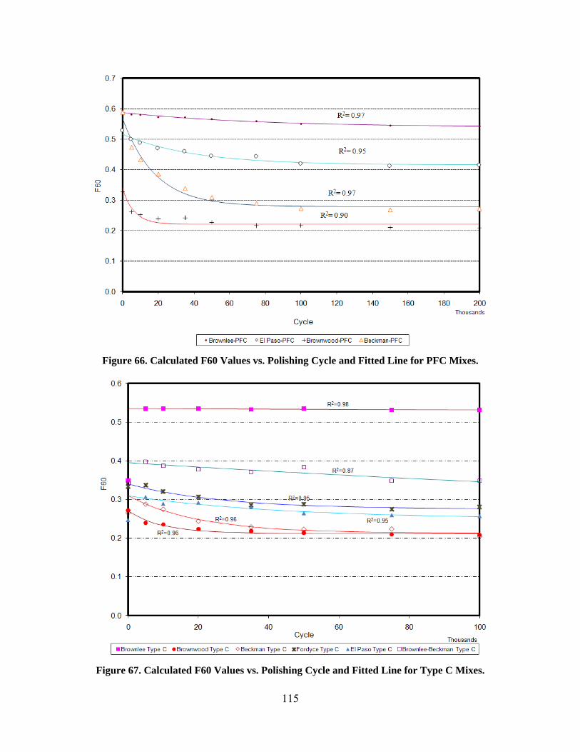
115
Figure 66. Calculated F60 Values vs. Polishing Cycle and Fitted Line for PFC Mixes.
Figure 67. Calculated F60 Values vs. Polishing Cycle and Fitted Line for Type C Mixes.
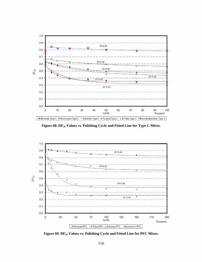
116
Figure 68. DF20 Values vs. Polishing Cycle and Fitted Line for Type C Mixes.
Figure 69. DF20 Values vs. Polishing Cycle and Fitted Line for PFC Mixes.
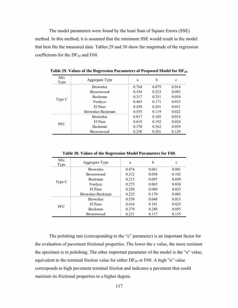
117
The model parameters were found by the least Sum of Square Errors (SSE)
method. In this method, it is assumed that the minimum SSE would result in the model
that best fits the measured data. Tables 29 and 30 show the magnitude of the regression
coefficients for the DF20 and F60.
Table 29. Values of the Regression Parameters of Proposed Model for DF20. Mix Type Aggregate Type a b c
Type C
Brownlee 0.764 0.079 0.014 Brownwood 0.354 0.223 0.093
Beckman 0.317 0.251 0.054 Fordyce 0.465 0.171 0.033 El Paso 0.430 0.201 0.031
Brownlee-Beckman 0.555 0.119 0.022
PFC
Brownlee 0.817 0.105 0.014 El Paso 0.619 0.192 0.024
Beckman 0.370 0.562 0.059 Brownwood 0.258 0.201 0.129
Table 30. Values of the Regression Model Parameters for F60. Mix Type Aggregate Type a b c
Type C
Brownlee 0.474 0.061 0.001 Brownwood 0.212 0.058 0.102
Beckman 0.213 0.097 0.050 Fordyce 0.275 0.065 0.038 El Paso 0.250 0.060 0.023
Brownlee-Beckman 0.225 0.170 0.003
PFC
Brownlee 0.539 0.048 0.013 El Paso 0.416 0.101 0.025
Beckman 0.279 0.288 0.055 Brownwood 0.221 0.117 0.155
The polishing rate (corresponding to the “c” parameter) is an important factor for
the evaluation of pavement frictional properties. The lower the c value, the more resistant
the specimen is to polishing. The other important parameter of the model is the “a” value,
equivalent to the terminal friction value for either DF20 or F60. A high “a” value
corresponds to high pavement terminal friction and indicates a pavement that could
maintain its frictional properties to a higher degree.

118
Figures 70 through 75 depict the values shown in Tables 29 and 30. These figures
indicate that the variation of both F60 and DF20 are consistent. In both cases, the
Brownlee aggregate has the highest terminal and initial values, and Beckman and
Brownwood aggregates have the lowest values. These figures also indicate that normally
PFC mixes normally have higher F60 terminal and initial values than the Type C does.
The rate of F60 change in Beckman and Brownwood aggregates is greater than other
types of aggregates, which shows that limestone aggregates are not able to maintain their
initial frictional properties against polishing action.
Figure 70. Terminal F60 Values for Different Aggregate Types.

119
Figure 71. Rate of F60 Change for Different Aggregate Types.
Figure 72. Initial F60 Values for Different Aggregate Types.
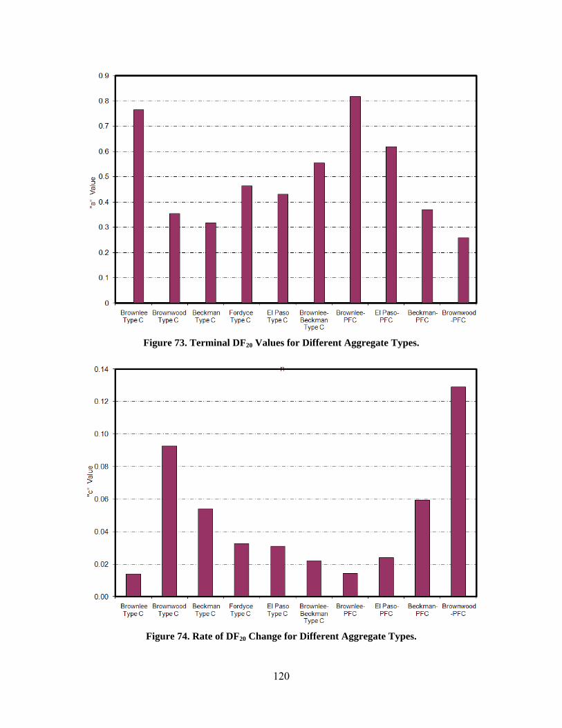
120
Figure 73. Terminal DF20 Values for Different Aggregate Types.
Figure 74. Rate of DF20 Change for Different Aggregate Types.
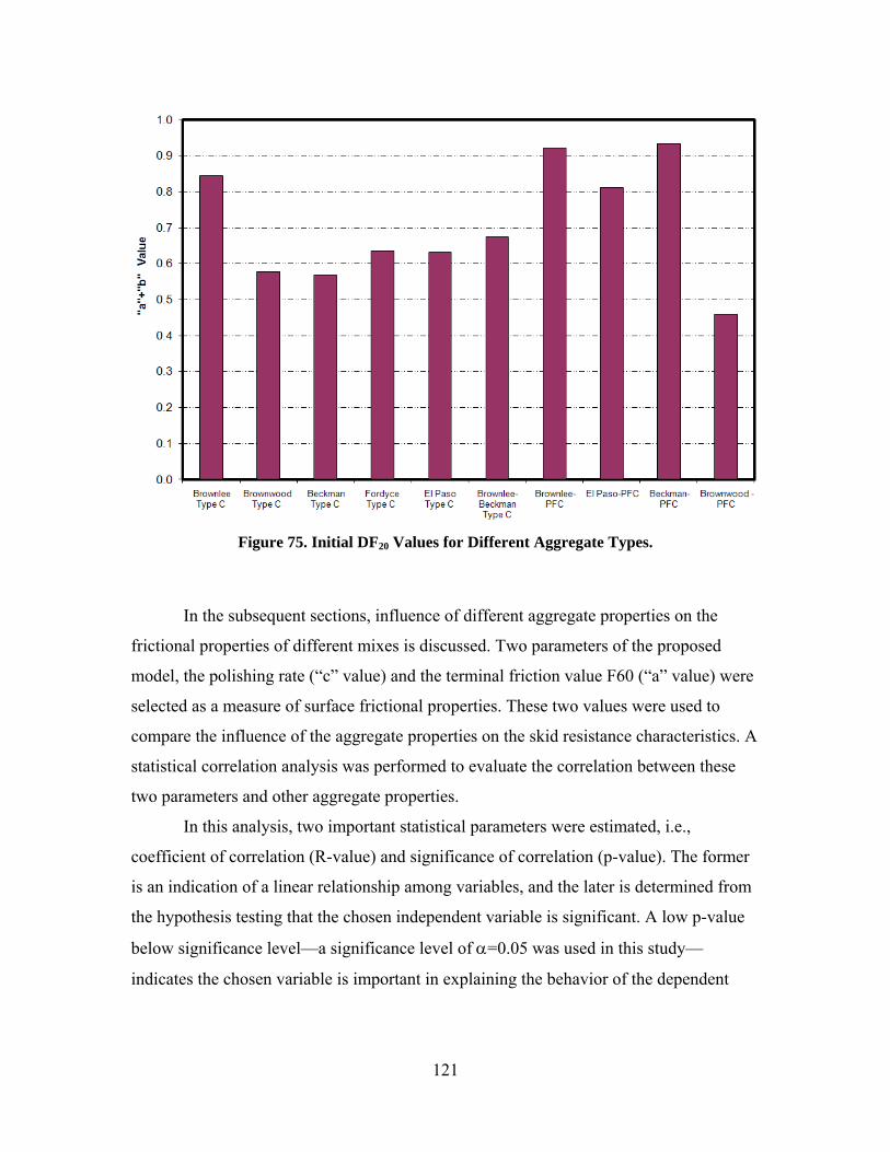
121
Figure 75. Initial DF20 Values for Different Aggregate Types.
In the subsequent sections, influence of different aggregate properties on the
frictional properties of different mixes is discussed. Two parameters of the proposed
model, the polishing rate (“c” value) and the terminal friction value F60 (“a” value) were
selected as a measure of surface frictional properties. These two values were used to
compare the influence of the aggregate properties on the skid resistance characteristics. A
statistical correlation analysis was performed to evaluate the correlation between these
two parameters and other aggregate properties.
In this analysis, two important statistical parameters were estimated, i.e.,
coefficient of correlation (R-value) and significance of correlation (p-value). The former
is an indication of a linear relationship among variables, and the later is determined from
the hypothesis testing that the chosen independent variable is significant. A low p-value
below significance level—a significance level of α=0.05 was used in this study—
indicates the chosen variable is important in explaining the behavior of the dependent

122
variable. Furthermore, this parameter shows if there is any significant statistical
correlation between parameters.
Hence, different aggregate characteristics discussed in previous chapters were
considered as the main aggregate characteristics affecting the frictional characteristics.
To explain the effect of each aggregate’s properties, a linear regression analysis was
done, and the significance of the regression coefficients was studied. Figures 99 to 134 in
Appendix C show the variation of F60 and DF20 terminal and change values against
different aggregate properties for Type C and PFC mixes.
Tables 31 and 32 summarize the regression coefficients and the results of the
statistical test on significance of the regression parameters for Type C and PFC mixes.
Table 31. Results of Regression Analysis on Type C Mix.
Mixture Frictional
Characteristics
Aggregate Properties
LA % Wt Loss Mg. Soundness Polish Stone Value MD % Wt. Loss Acid Insolubility
R2 p-value R2 p-value R2 p-value R2 p-value R2 p-value
DF20 Change 0.01 0.45 0.09 0.28 0.67 0.02 0.01 0.45 0.43 0.08 DF20 Terminal 0.14 0.23 0.01 0.43 0.90 0.00 0.00 0.50 0.38 0.09 F60 Change 0.00 0.45 0.09 0.28 0.68 0.02 0.05 0.33 0.27 0.14 F60 Terminal 0.16 0.22 0.01 0.43 0.70 0.02 0.01 0.44 0.35 0.11
Mixture Frictional
Characteristics
Aggregate Properties Texture Change BMD*
and AMD Angularity Change BMD
and AMD Texture AMD Angularity AMD
R2 p-value R2 p-value R2 p-value R2 p-value
DF20 Change 0.73 0.01 0.35 0.11 0.38 0.10 0.10 0.27 DF20 Terminal 0.69 0.02 0.84 0.01 0.62 0.03 0.00 0.46 F60 Change 0.64 0.03 0.32 0.12 0.37 0.10 0.02 0.39 F60 Terminal 0.44 0.08 0.64 0.03 0.53 0.05 0.01 0.43
* Before Micro-Deval
* After Micro-Deval

123
Table 32. Results of Regression Analysis on PFC Mix.
Mixture Frictional
Characteristics
Aggregate Properties
LA % Wt Loss Mg. Soundness Polish Stone Value
MD % Wt. Loss Acid Insolubility
R2 p-value R2 p-value R2 p-value R2 p-value R2 p-value
DF20 Change 0.05 0.39 0.43 0.17 0.55 0.13 0.07 0.32 0.63 0.10 DF20 Terminal 0.05 0.39 0.09 0.35 0.81 0.05 0.00 0.48 0.96 0.01 F60 Change 0.09 0.35 0.53 0.13 0.51 0.14 0.13 0.32 0.54 0.13 F60 Terminal 0.09 0.35 0.08 0.36 0.83 0.04 0.00 0.48 0.97 0.01
Mixture Frictional
Characteristics
Aggregate Properties Texture Change BMD and AMD
Angularity Change BMD and AMD Texture AMD Angularity AMD
R2 p-value R2 p-value R2 p-value R2 p-value
DF20 Change 0.61 0.11 0.10 0.34 0.42 0.18 0.35 0.20 DF20 Terminal 0.91 0.02 0.39 0.19 0.77 0.06 0.32 0.22 F60 Change 0.50 0.15 0.08 0.36 0.32 0.22 0.28 0.24 F60 Terminal 0.91 0.02 0.42 0.18 0.77 0.06 0.30 0.23
Tables 31 and 32 show a variety of aggregate properties assumed to have some
effects on the measured friction of different surfaces. These properties include:
• LA abrasion weight loss,
• Magnesium soundness test value,
• Polish Stone Value,
• Micro-Deval weight loss,
• coarse aggregate acid insolubility,
• terminal texture measured by AIMS after Micro-Deval,
• terminal angularity measured by AIMS after Micro-Deval,
• change in texture before and after micro-Deval measured by AIMS, and
• change in angularity before and after micro-Deval measured by AIMS.
These tables show that the LA abrasion value could explain less than 20 percent
variation in DF20 and F60 change, and the coefficient of regression is not significant at
95 percent confidence level. Therefore, the LA abrasion weight loss does not seem to be
a significant factor in pavement skid resistance. The same result could be concluded for
124
magnesium sulfate soundness value, Micro-Deval weight loss, and terminal angularity
after Micro-Deval. Moreover, R-squared values in both Type C and PFC mixes are very
low, and the p-value is higher than 0.05. The coarse aggregate acid insolubility value is
likely to be an important factor in both F60 and DF20 terminal values and rate of change,
although the R-squared values are not high in Type C mixes. The low R-squared value
might be due to data outliers. Further analysis was performed to investigate the effect of
coarse aggregate insolubility value without considering outliers. The results will be
discussed later in this chapter.
The results of analysis show that British Pendulum is a significant factor at
95 percent confidence level. The R-square values are about 0.6 for rate of change in both
Type C and PFC mixes and 0.8 for terminal values. This indicates BP value is more
important on terminal F60 and DF20 values. Moreover, the results of the analysis show
that the F60 and DF20 terminal values increase and F60 and DF20 rate of change decrease
when the British pendulum value increases.
Change in texture before and after Micro-Deval and the texture after Micro-Deval
are significant factors in terminal DF20 and F60 values and rate of change. Moreover,
change in texture before and after Micro-Deval accounts for 73 and 64 percent change in
DF20 and F60 variation, respectively, and is significant in Type C mixes. Texture change
before and after Micro-Deval accounts for a 91 percent change in DF20 and F60 terminal
value and is significant in PFC mixes. It is evident that the texture change has more
influence on DF20 than F60. This, in part, can be justified by the contribution of
macrotexture on calculating the F60 value that makes the F60 change less dependent on
microtexture than DF20. Measured texture after Micro-Deval defines 62 and 53 percent
change in DF20 and F60 terminal values and statistically is significant in Type C mixes.
In PFC mixes, the terminal texture value after the Micro-Deval test is responsible for
77 percent change in Df20 and F60 terminal values and is significant. As a general trend,
an increase in terminal texture will result in an increase in DF20 and F60 terminal values
and a decrease in DF20 and F60 rate of change. The same effect could be seen in texture
change before and after Micro-Deval. Increase in texture change before and after
Micro-Deval decreases the terminal value of DF20 and F60 and increases their rate of
change.

125
Change in angularity before and after Micro-Deval affects the terminal DF20 and
F60 values. When the angularity change before and after Micro-Deval increases, the
terminal F60 and DF20 values increase.
Since Brownlee aggregate had very high microtexture that might affect the results
of the analysis, the mixes containing Brownlee aggregate were removed from the
database and another analysis was performed. Figures 135 through 140 in Appendix C
show the results of the analysis conducted without sandstone. Table 33 summarizes the
estimated R-squared values and significance level of considered parameter in the
analysis.
Table 33. R-squared Values and Significant Level for Type C Mix.
Mixture Frictional
Characteristics
Aggregate properties
LA % Wt Loss Mg. Soundness MD % Wt. Loss
R2 p-value R2 p-value R2 p-value
F60 Change 0.05 0.36 0.19 0.23 0.04 0.37
F60 Terminal 0.36 0.14 0.31 0.16 0.59 0.06
Mixture Frictional
Characteristics
Aggregate properties Acid
Insolubility Texture Change BMD and AMD
Angularity AMD
R2 p-value R2 p-value R2 p-value
F60 Change 0.17 0.24 0.55 0.08 0.06 0.34
F60 Terminal 0.83 0.02 0.59 0.06 0.97 0.00
This analysis revealed that LA weight loss and magnesium soundness values are
not statistically significant in predicting the DF20 and F60 terminal values and rate of
change. However, this analysis showed that the coarse aggregate insolubility value is a
significant factor on the terminal F60 value and could explain the 83 percent change in
F60. This analysis also showed that angularity after Micro-Deval is also a statistically
significant factor on explaining the F60 terminal values. Moreover, the terminal F60
value increases when angularity after Micro-Deval increases. Similarly, an increase in
coarse aggregate acid insoluble value increases terminal F60 value.
126
AGGREGATE RANKING BASED ON LAB RESULTS
Selection of an aggregate type based on its frictional properties is an important
step toward constructing a safe pavement with adequate skid resistance. A ranking
system according to frictional properties will assist the selection of the most appropriate
aggregate. The frictional properties of each aggregate type could be assessed by using
friction-polish cycle curve. ANOVA analysis was done to study the effect of mix type
and aggregate on the measured F60. It was demonstrated that the difference between the
measured F60 values of Type C and PFC mixes is significant. Moreover, any aggregate
classification system that tends to classify aggregates should consider the mix type as an
important factor.
Figure 76 shows the terminal F60 values of different aggregate for different
mixes. This figure shows the Brownlee aggregate had superior frictional performance in
both Type C and PFC mixes. The results of the ANOVA analysis in the previous section
showed that there is a significant difference between measured F60 values of Brownlee
aggregate and other aggregates. This result is in agreement with the result of TxDOT
aggregate classification that considers Brownlee aggregate in class A. The next aggregate
in the list is El Paso aggregate that has been used in PFC mixes. This aggregate, however,
does not have high terminal friction in Type C. The El Paso aggregate in the PFC mixture
also had significant differences with all other aggregates and was the third in the list.
Mixing 50 percent Brownlee aggregate with 50 percent Beckman aggregate gives
the blend superior frictional properties. Although the blend is classified B based on the
current classification system, the frictional properties of the blend are significantly better
than Fordyce aggregate and El Paso in Type C mixture.
Beckman aggregate shows relatively good frictional properties in PFC mixes.
Beckman aggregate has a high amount of carbonate material that is abraded quickly from
the surface of the aggregate, fills the pores of PFC mixture in the lab experiment, and
improves the skid resistance of the mix. This effect, however, could lead to a decrease in
permeability.

127
Figure 76. Mean F60 Values for Different Aggregate Types.
Although Fordyce aggregate is the next in the group and has slightly better
frictional properties than El Paso aggregate, the difference is not significant. El Paso
aggregate showed better frictional characteristics than Beckman and Brownwood
aggregates.
Using Brownwood aggregate in the PFC mixture gives the mix slightly better
frictional performance than Type C. No significant differences were observed in
frictional properties of Beckman and Brownwood aggregate.
El P
aso
Type
C
Ford
yce
Type
C
Bro
wnw
ood
Type
C
Bro
wnl
ee T
ype
C
Bec
kman
Typ
e C
Bro
wnl
ee a
nd
Bec
kman
Typ
e C
El P
aso
PFC
Bro
wnw
ood
PFC
Bro
wnl
ee P
FC
Bec
kman
PFC
Mea
n F6
0
0.2
0.3
0.4
0.5
0.6


129
CHAPTER V – MIX FRICTION MODEL BASED ON AGGREGATE PROPERTIES
INTRODUCTION
This chapter presents a new model that expresses F60 values as a function of
aggregate resistance to polishing and gradation. This model will assist in predicting the
frictional performance of a road and select corrective measures to improve it. Figure 77
shows an overview of the friction model.
Figure 77. Overview of the Friction Model.
The friction model shown in Figure 77 consists of a set of equations that can
predict F60 value at any given polishing level. Moreover, this model should predict three
important parameters—initial F60 level (“a” + “b”), rate of F60 change “c,” and terminal
F60 value “a.”
MODELING APPROACH
The previous chapter showed the mixture type; namely aggregate gradation has a
significant effect on F60 parameters. To consider the aggregate gradation as a parameter
in the friction model, a cumulative two-parameter Weibull distribution was used to fit the
standard aggregate size distribution data (cumulative percent passing size). The
cumulative two-parameter Weibull distribution has the form of:
Aggregate Properties e.g., Gradation AIMS Indices
Cumulative Number of Traffic
Model Predicted F60
Input Output
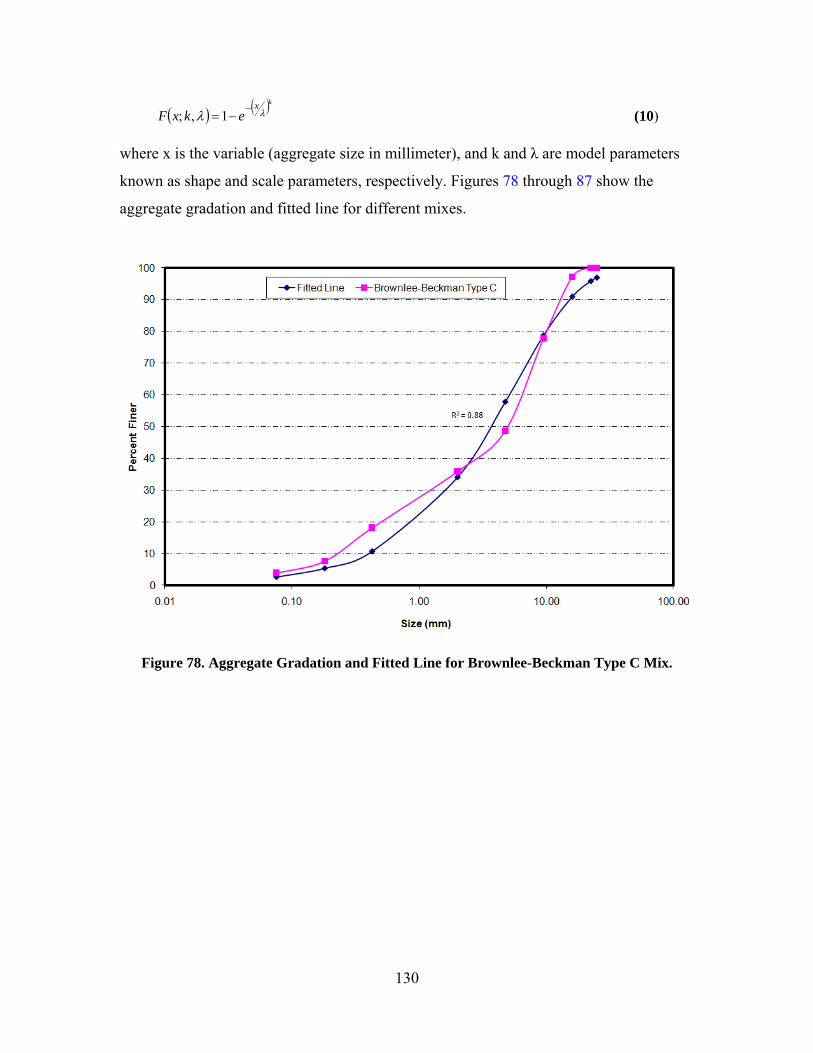
130
( ) ( )kxekxF λλ
−−=1,; (10)
where x is the variable (aggregate size in millimeter), and k and λ are model parameters
known as shape and scale parameters, respectively. Figures 78 through 87 show the
aggregate gradation and fitted line for different mixes.
Figure 78. Aggregate Gradation and Fitted Line for Brownlee-Beckman Type C Mix.
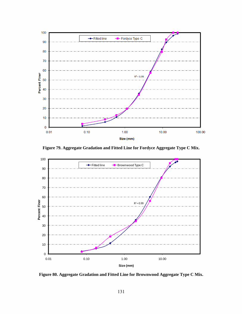
131
Figure 79. Aggregate Gradation and Fitted Line for Fordyce Aggregate Type C Mix.
Figure 80. Aggregate Gradation and Fitted Line for Brownwood Aggregate Type C Mix.
0
10
20
30
40
50
60
70
80
90
100
0.01 0.10 1.00 10.00
Perc
ent
Fine
r
Size (mm)
Fitted line Brownwood Type C
R2 = 0.99
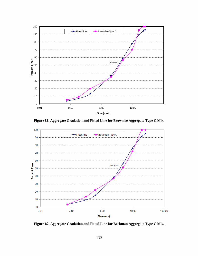
132
Figure 81. Aggregate Gradation and Fitted Line for Brownlee Aggregate Type C Mix.
Figure 82. Aggregate Gradation and Fitted Line for Beckman Aggregate Type C Mix.
0
10
20
30
40
50
60
70
80
90
100
0.01 0.10 1.00 10.00
Perc
ent
Fine
r
Size (mm)
Fitted line Brownlee Type C
R2 = 0.98

133
Figure 83. Aggregate Gradation and Fitted Line for El Paso Aggregate Type C Mix.
Figure 84. Aggregate Gradation and Fitted Line for Brownwood Aggregate PFC Mix.
0
10
20
30
40
50
60
70
80
90
100
0.01 0.10 1.00 10.00
Perc
ent
Fine
r
Size (mm)
Fitted line Brownwood PFC
R2 = 0.99

134
Figure 85. Aggregate Gradation and Fitted Line for Beckman Aggregate PFC Mix.
Figure 86. Aggregate Gradation and Fitted Line for Brownlee Aggregate PFC Mix.
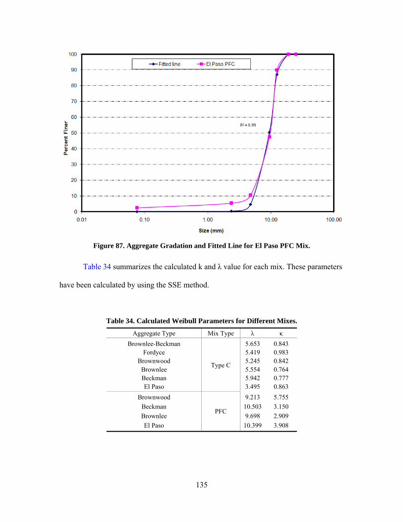
135
Figure 87. Aggregate Gradation and Fitted Line for El Paso PFC Mix.
Table 34 summarizes the calculated k and λ value for each mix. These parameters
have been calculated by using the SSE method.
Table 34. Calculated Weibull Parameters for Different Mixes. Aggregate Type Mix Type λ κ
Brownlee-Beckman
Type C
5.653 0.843 Fordyce 5.419 0.983
Brownwood 5.245 0.842 Brownlee 5.554 0.764 Beckman 5.942 0.777 El Paso 3.495 0.863
Brownwood
PFC
9.213 5.755 Beckman 10.503 3.150 Brownlee 9.698 2.909 El Paso 10.399 3.908

136
The results of the previous chapter showed the AIMS texture indices have a high
correlation with rate of change and terminal values of F60, and this value could be
potentially used in any model explaining the F60. Selecting other aggregate properties
that can be used in the model should be based on a statistical analysis. This analysis will
show the minimum number of independent variables that can be used in the model. Any
correlation between the independent variables will decrease the reliability of the model.
Table 35 shows the cross correlation between different parameters considered to be
significant in the model. This table shows that the “a” (terminal value), “c” (rate of
change), and “a” + “b” (initial value)—parameters of aggregate texture model—have
high correlation with polish value, texture after Micro-Deval, texture change before and
after Micro-Deval, and coarse aggregate acid insolubility. This analysis shows that
developing a model that includes parameters of the aggregate texture model proposed by
Mahmoud (2005) along with aggregate gradation parameters could satisfactorily explain
the variation of F60 for different mixtures without any redundancy and cross correlation.
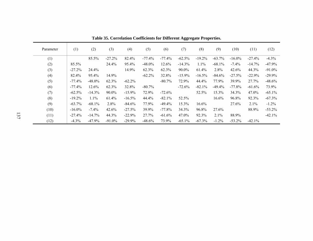
137
Table 35. Correlation Coefficients for Different Aggregate Properties.
Parameter (1) (2) (3) (4) (5) (6) (7) (8) (9) (10) (11) (12)
(1) 85.5% -27.2% 82.4% -77.4% -77.4% -62.5% -19.2% -63.7% -16.0% -27.4% -4.3% (2) 85.5% 24.4% 95.4% -48.0% 12.6% -14.3% 1.1% -68.1% -7.4% -14.7% -47.9% (3) -27.2% 24.4% 14.9% 62.3% 62.3% 90.0% 61.4% 2.8% 42.6% 44.3% -91.0% (4) 82.4% 95.4% 14.9% -62.2% 32.8% -15.9% -16.5% -84.6% -27.5% -22.9% -29.9% (5) -77.4% -48.0% 62.3% -62.2% -80.7% 72.9% 44.4% 77.9% 39.9% 27.7% -48.6% (6) -77.4% 12.6% 62.3% 32.8% -80.7% -72.6% -82.1% -49.4% -77.8% -61.6% 73.9% (7) -62.5% -14.3% 90.0% -15.9% 72.9% -72.6% 52.5% 15.3% 34.3% 47.0% -65.1% (8) -19.2% 1.1% 61.4% -16.5% 44.4% -82.1% 52.5% 16.6% 96.8% 92.3% -67.3% (9) -63.7% -68.1% 2.8% -84.6% 77.9% -49.4% 15.3% 16.6% 27.6% 2.1% -1.2%
(10) -16.0% -7.4% 42.6% -27.5% 39.9% -77.8% 34.3% 96.8% 27.6% 88.9% -53.2% (11) -27.4% -14.7% 44.3% -22.9% 27.7% -61.6% 47.0% 92.3% 2.1% 88.9% -42.1% (12) -4.3% -47.9% -91.0% -29.9% -48.6% 73.9% -65.1% -67.3% -1.2% -53.2% -42.1%

138
where:
(1) LA weight loss (percent),
(2) Mg. weight loss (percent),
(3) Polish Stone Value,
(4) Micro-Deval weight loss (percent),
(5) coarse aggregate acid insolubility,
(6) change in texture before and after Micro-Deval,
(7) change in angularity before and after Micro-Deval,
(8) texture after Micro-Deval,
(9) angularity after Micro-Deval,
(10) terminal texture for aggregates (“aagg” value),
(11) initial texture for aggregates (“aagg” + “bagg”), and
(12) rate of texture change for aggregates (“cagg” value).
A nonlinear regression analysis was performed to determine the coefficients for
model parameters. Table 36 shows parameter estimates for the model.
Table 36. Different Parameter of the Friction Model Estimated by Regression Analysis.
Parameter Model R2
Terminal F60
(amix)
0.96
Initial F60 (amix + bmix)
( )( ) 8.010985.410846.510656.5ln4984.0 224 +×−×++× −−− kba aggagg λ
0.82
F60 Rate of Change (cmix)
⎟⎠
⎞⎜⎝
⎛ ⋅− −
⋅ aggce210297.7
765.0 0.90
where:
AMD: Aggregate texture after Micro-Deval,
“aagg” + “bagg”: Aggregate initial texture using texture model,
cagg : Aggregate texture rate of change using texture model,
( )20013.0936.118422.18
AMD×−+ λ

139
k-value: Weibull distribution shape factor, and
λ-value: Weibull distribution scale factor.
The developed model for the terminal F60 value is significant at 95 percent confidence
level. This model consists of the aggregate terminal texture value measured after
Micro-Deval and λ-value related to mix gradation. Researchers noted that this model has
a high R-square and can account for 96 percent of the variation in terminal F60.
Figure 88 shows the predicted terminal F60 values versus measured terminal F60
values. Based on this model, a higher texture after Micro-Deval will result in a higher
terminal value for F60. Likewise, the mixes with high λ-values—primarily PFC
mixes—have higher terminal F60 values.
Table 36 also shows the initial F60 value is depending on the aggregate initial
texture value (“aagg” + “bagg”), which is calculated by fitting a model to a texture and
corresponding gradation parameters k-value and λ-value. The model is significant overall
and has a high R-square of 0.82. Figure 89 depicts the measured and predicted initial F60
values.
The rate of F60 change in Table 36 is only depending on the rate of texture
change in corresponding aggregate. The model is significant, and the R-square is 0.91.
Figure 90 shows the predicted and measured rate of F60 change (“c” value).
Figure 88. Predicted vs. Measured Terminal F60 Values.
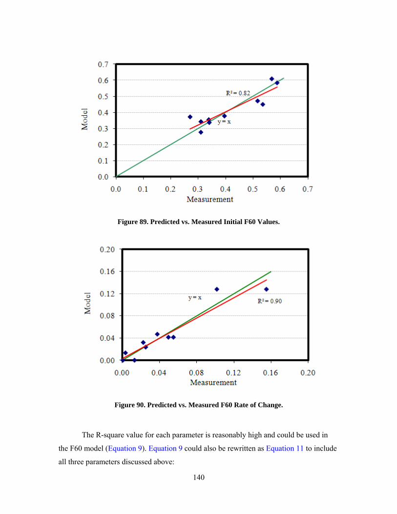
140
Figure 89. Predicted vs. Measured Initial F60 Values.
Figure 90. Predicted vs. Measured F60 Rate of Change.
The R-square value for each parameter is reasonably high and could be used in
the F60 model (Equation 9). Equation 9 could also be rewritten as Equation 11 to include
all three parameters discussed above:
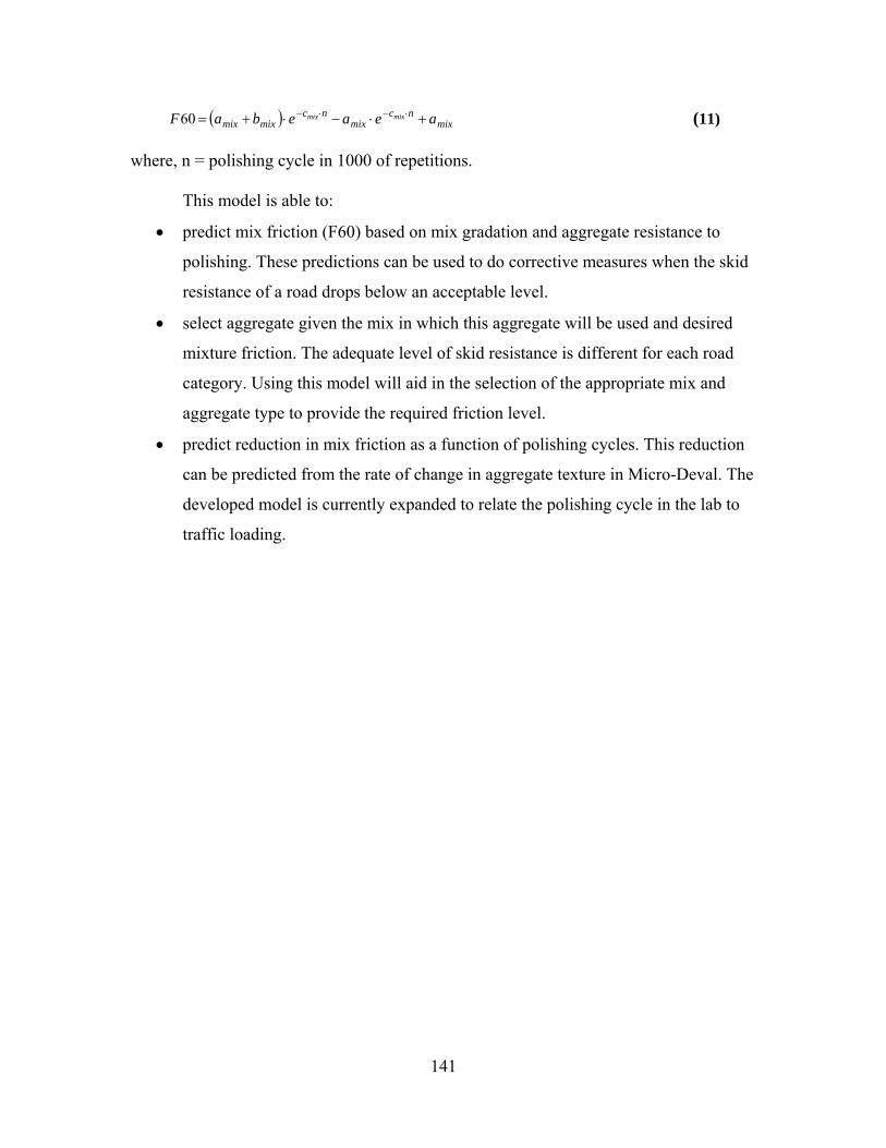
141
( ) mixnc
mixnc
mixmix aeaebaF mixmix +⋅−⋅+= ⋅−⋅−60 (11)
where, n = polishing cycle in 1000 of repetitions.
This model is able to:
• predict mix friction (F60) based on mix gradation and aggregate resistance to
polishing. These predictions can be used to do corrective measures when the skid
resistance of a road drops below an acceptable level.
• select aggregate given the mix in which this aggregate will be used and desired
mixture friction. The adequate level of skid resistance is different for each road
category. Using this model will aid in the selection of the appropriate mix and
aggregate type to provide the required friction level.
• predict reduction in mix friction as a function of polishing cycles. This reduction
can be predicted from the rate of change in aggregate texture in Micro-Deval. The
developed model is currently expanded to relate the polishing cycle in the lab to
traffic loading.

143
CHAPTER VI – RESULTS AND CONCLUSIONS
INTRODUCTION
During the course of this study, the frictional behavior of different aggregates and
mixture types were measured and analyzed. Several asphalt mix slabs were prepared and
compacted in the lab, and their frictional properties were measured using the sand patch
method, British Pendulum Test, Dynamic Friction Test, and Circular Texture Meter. The
results of each test are summarized in this chapter.
SAND PATCH TEST
This test was performed on Type C and Type D mixes only. Comparing the mean
MTD values of these two mixes before polishing showed that the average MTD values of
Type C mixes were greater than those for Type D mixes. This is due to the larger
maximum aggregate size in the Type C mix, which can result in a higher macrotexture
before polishing.
Although it seemed as if the MTD values of almost all mixes (except for
sandstone) after polishing were less than the MTD values before polishing, statistical
analysis did not show any significant differences between MTD values before and after
polishing. Hence, researchers concluded that the sand patch test was not able to detect
changes in macrotexture due to polishing with the selected polishing device. The results
showed that mixes with different aggregates had different MTD values. Thus, a pairwise
comparison analysis was performed between the aggregates to find the differences
between MTD values of different aggregate types. The results showed that Brownlee
aggregate had the highest MTD values among all aggregates, and both Beckman and
Brownwood aggregates produced the lowest MTD values.
BRITISH PENDULUM TEST
This test was performed on three different locations on each slab, and three
measurements were conducted on each location. The TxDOT test requires using a 3-inch
slider in the BP. However, it was not feasible to use this size because of the limited
144
polished area resulting from the polished machine used in this study. As a result, a
1.5-inch wide rubber slider was used in all BP measurements.
The results indicated that BP values decreased with an increase in polishing
cycles for all aggregates except mixtures containing Brownlee aggregate. For Brownlee
aggregate, the BP values remained almost constant
The BP values of PFC mixes were generally higher than those for Type C mixes.
In addition, the frictional characteristics of some aggregates varied depending on the mix
in which the aggregate was used. It is interesting to note that, for example, the PFC and
Type C mixes with Brownwood aggregate had similar BP values at a low number of
polishing cycles. However, the PFC with Brownwood aggregate had higher BP values
than Type C at a high number of polishing cycles.
An analysis was performed to compare the results of measured BP values for each
aggregate type. The results of the comparison between two aggregate types did not reveal
any significant differences. Consequently, the British Pendulum test was not able to
detect the difference between frictional performances of aggregates with a known
difference in frictional characteristics.
CTMETER AND DFT TESTS
These two tests were performed at three different locations on each slab. The DFT
was performed twice in each location while the CTMeter was conducted six times at each
location. No particular trend was observed for MPD values from CTMeter of different
mixes in terms of polishing cycles.
The result of dynamic friction testing at 20 km/h (DF20) is an indication of
microtexture (Hall et al., 2006). Therefore, this measure is a good indication of aggregate
contribution to pavement skid properties. A plot of measured dynamic friction in terms of
polishing cycles showed that DF20 decreased as polishing cycles increased. The DF20
curves leveled off and reached a terminal value after a certain number of polishing
cycles.
Statistical analysis was performed to evaluate the effect of several variables (i.e.,
aggregate type, mix type, polishing cycles, and speed) on the measured dynamic friction.
The results showed aggregate type affected the magnitude of dynamic friction in both

145
Type C and PFC mixes. The results also showed that there was a significant difference in
the measured friction at different numbers of polishing cycles for Type C mixes. On the
contrary, the magnitude of dynamic friction in PFC mixes did not have a significant
difference between polishing cycles. The results also revealed that the PFC mix has a
higher friction value than Type C mix.
The equation proposed by Mahmoud (2005) was fitted to the calculated F60
values. The rate of change and terminal value of friction were estimated from this
equation. Comparing the rate of change and terminal values for different aggregates
revealed that in all cases the Brownlee aggregate had the highest terminal values and
lowest rate of change in both Type C and PFC mixes. On the contrary, mixes containing
Beckman and Brownwood aggregates had the lowest terminal values and highest rate of
change. This indicated that Beckman and Brownwood aggregates failed to preserve their
frictional performance during load application. A combination of Brownlee and Beckman
aggregates, however, performed satisfactorily and had a high terminal value and low rate
of change compared to the Beckman aggregate. Fordyce and El Paso aggregates were
almost the same and had fair frictional properties.
The dependency of terminal value and rate of change of DF20 and F60 on different
aggregate characteristics was analyzed. The aggregate characteristics included in the
analysis were LA impact and abrasion percent weight loss, magnesium soundness percent
weight loss, British Pendulum value, Micro-Deval percent weight loss, coarse aggregate
acid insolubility, texture measurements after Micro-Deval by AIMS, angularity
measurements after Micro-Deval by AIMS, change in texture before and after
Micro-Deval, and change in angularity before and after Micro-Deval. The coefficient of
determination (R-square) and the statistical significance were evaluated to study if the
considered variable is important and at what percent it could define the variability of
DF20 and F60.
The results indicated that the LA impact and abrasion percent weight loss,
magnesium soundness percent weight loss, Micro-Deval percent weight loss, angularity
measurements after Micro-Deval by AIMS, and change in angularity before and after
Micro-Deval were not significant factors in determining DF20 and F60 rate and terminal
values.

146
British Pendulum value, texture after Micro-Deval by AIMS, and change in
texture before and after Micro-Deval were proved to be significant factors in explaining
the rate and terminal values of DF20 and F60. Furthermore, the rate of DF20 and F60
decreased as the stone BP value and texture after Micro-Deval increased. In addition, the
terminal value of DF20 and F60 increased as the BP value and texture after Micro-Deval
increased. The rate of change in texture before and after Micro-Deval affected the rate
and terminal values of DF20 and F60. The results show the rate of change in DF20 and F60
decreases and the terminal value increases as she rate of change in texture before and
after Micro-Deval decreases. The coarse aggregate acid insolubility test showed a
significant effect on rate and terminal values of DF20 and F60 only when Brownlee
aggregate was removed from the comparison. In such a case, the terminal DF20 and F60
increased as the acid insolubility test value increased. Change in angularity before and
after Micro-Deval affects the terminal DF20 and F60 values. When the angularity change
before and after Micro-Deval increased, the terminal F60 and DF20 values increased.
SUMMARY
In summary, the results of the research indicated that it is possible to control and
predict frictional properties of the pavement by selecting the aggregate type and HMA
mix type. A new laboratory testing methodology to evaluate the key parameters in
frictional characteristics of a flexible pavement was developed. These two key parameters
were defined to be the rate of decrease in friction and terminal value for friction. These
two values could be used as a basis for further comparisons between frictional
performances of different aggregate types.
During this study, a complete set of experiments was performed to evaluate the
aggregate properties by all current testing methods. The results of this research confirmed
the findings of the previous research about the superior performance of the Brownlee
aggregate. The results also showed the polishing susceptibility of Beckman and
Brownwood aggregates.
The influence of the aggregate type on asphalt concrete skid properties was
investigated through preparing and testing laboratory slabs. The results of the analysis
confirmed the strong relationship between mix frictional properties and aggregate
147
properties. The main aggregate properties affecting the mix skid resistance were
recognized to be British Pendulum value, texture change before and after Micro-Deval
measured by AIMS, terminal texture after Micro-Deval measured by AIMS, and coarse
aggregate acid insolubility value. Based on the findings, a model that is able to predict
initial F60, terminal F60, and rate of polishing was developed using the parameters in the
texture model developed by Mahmoud (2005). This model confirmed the benefits of
texture measurements by AIMS. This model will help to predict mix friction based on
gradation and aggregate resistance to polishing. This model also facilitates selecting the
appropriate aggregate type for the desired mixture friction. This model could also be used
to classify aggregates based on their frictional properties.

149
REFERENCES Abdul-Malak, M.A.U., Meyer, A.H., and Fowler, D.W. 1990. Research Program for
Predicting the Frictional Characteristics of Seal-Coat Pavement Surface.
Transportation Research Record 1217, Transportation Research Board, TRB,
National Research Council, Washington, D.C.
Abe, H., Henry, J.J., Tamai, A., and Wambold, J. 2000. Measurement of Pavement
Macrotexture Using the CTMeter. Transportation Research Record 1764,
Transportation Research Board, TRB, National Research Council, Washington, D.C.
Agrawal S.K. and Henry, J.J. 1979. Technique for Evaluating Hydroplaning Potential of
Pavements. Transportation Research Record 633, Transportation Research Board,
TRB, National Research Council, Washington, D.C.
Ahammed A.M. and Tighe S.L. 2007. Evaluation of Concrete Pavement’s Surface
Friction Using LTPP Data: Preliminary Analysis and Texture Performance Models.
Proceedings of the 86th Transportation Research Board Annual Meeting (CD),
Washington, D.C., January.
Al-Rousan, T.M. 2004. Characterization of Aggregate Shape Properties Using a
Computer Automated System. Ph.D. Dissertation, College Station, TX.
Alvarado, C., Mahmoud, E., Abdullah, I., Masad, E., Nazarian, S., Tandon, J., and
Button, J. 2006. Feasibility of Quantifying the Role of Coarse Aggregate Strength on
Resistance to Load in HMA. Center for Transportation Infrastructure Systems,
University of Texas at El Paso, Research Report 0-5268-2, October.
Anderson, D.A., Meyer, W.E., and Rosenberger, J.L. 1986. Development of a Procedure
for Correcting Skid-Resistance Measurements to a Standard End-of-Season Value.
Transportation Research Record, No. 1084. Transportation Research Board, TRB,
National Research Council, Washington, D.C.
ASTM. 2007. Annual Book of ASTM Standards, Vol. 04.03, American Society for
Testing and Materials, West Conshohocken, PA.
Balmer, G.G. and Colley, B.E. 1966. Laboratory Studies of the Skid Resistance of
Concrete. American Society for Testing and Materials, Journal of Materials,
Vol. 1-No. 3.

150
Balmer, G.G. 1978. Pavement Texture: Its Significance and Development.
Transportation Research Record 666. Transportation Research Board, TRB, National
Research Council, Washington, D.C.
Bituminous Rated Sources Quality Catalogue (BRSQC). 2008. Texas Department of
Transportation, ftp://ftp.dot.state.tx.us/pub/txdot-info/cmd/mpl/brsqc.pdf. Access date:
6/29/08.
Bloem, D.L. 1971. Skid-Resistance: The Role of Aggregates and Other Factors. National
Sand and Gravel Association Circular 109, Silver Spring, MD.
Bond, R., Katekhda, I.E.D., Lees, G., and Williams, A.R. 1976. Tire/Road Surface
Interaction. Journal of the Institution of Highway Engineers, November.
Bray, J. 2002. The Role of Crash Surveillance and Program Evaluation: NYSDOT’s Skid
Accident Reduction Program (SKARP). Presented at 28th International Forum on
Traffic Records and Highway Information System, Orlando, FL.
Britishpendulum. 2008. http://www.Britishpendulum.co.uk/. Access date: 2/23/08.
Burnett, W.C., Gibson, J.L., and Kearney, E.J. 1968. Skid Resistance of Bituminous
Surfaces. Highway Research Record, No. 236, Highway Research Board, National
Research Council, Washington, D.C.
Cairney, P. 1997. Skid Resistance and Crashes – A Review of the Literature. Research
Report No. 311, ARRB Transport Research Ltd., Vermont South Victoria, Australia.
Cenek, P.D., Davies, R.B., McLarin, M.W., and Griffith-Jones, N.J. 1997. Road
Environment and Traffic Crashes. Transfund Research Report No. 79, Transfund
New Zealand, Wellington, New Zealand.
Chelliah, T., Stephanos P., Shah, M.G., and Smith, T. 2003. Developing a Design Policy
to Improve Pavement Surface Characteristics. Presented in Transportation Research
Board 82nd Annual Meeting, Washington, D.C.
Choubane, B., Holzschuher, C.R., and Gokhale, S. 2004. Precision of Locked-Wheel
Testers for Measurement of Roadway Surface Friction Characteristics.
Transportation Research Record 1869, Transportation Research Board, TRB,
National Research Council, Washington, D.C.

151
Colony, D.C. 1986. Overview of Skid Resistance on Ohio Pavements. Journal of
Transportation Engineering, American Society of Civil Engineers, ASCE,
September.
Cooley, L., Jr. and James, R. 2003. Micro-Deval Testing of Aggregates in the Southeast.
Transportation Research Record 1837, Transportation Research Board, TRB,
National Research Council, Washington, D.C.
Crouch, L.K., Shirley, G., Head, G., and Goodwin, W.A. 1996. Aggregate Polishing
Resistance Pre-Evaluation. Transportation Research Record 1530, Transportation
Research Board, TRB, National Research Council, Washington, D.C.
Csathy, T.I., Burnett, W.C., and Armstrong, M.D. 1968. State-of-the-Art of Skid
Resistance Research. Highway Research Board Special Report 95, Highway
Research Board, National Research Council, Washington, D.C.
Dahir, S.H., Meyer, W.E., and Hegmon, R.R. 1976. Laboratory and Field Investigation of
Bituminous Pavement and Aggregate Polishing. Transportation Research Record
584, Transportation Research Board, TRB, National Research Council,
Washington, D.C.
Dahir, S. 1979. A Review of Aggregate Selection Criteria for Improved Wear Resistance
and Skid Resistance of Bituminous Surfaces. Journal of Testing and Evaluation,
Vol. 7.
Dames, J. 1990. The Influence of Polishing Resistance of Sand on Skid Resistance of
Asphalt Concrete. Surface Characteristics of Roadways: International Research and
Technologies, ASTM STP 1031, W.E. Meyer, and J. Reichert, Eds., American
Society for Testing and Materials, Philadelphia, PA.
Davis, R.M., Flintsch, G.W., Al-Qadi, I.L.K., and McGhee, K. 2002. Effect of Wearing
Surface Characteristics on Measured Pavement Skid Resistance and Texture.
Presented at 81st Transportation Research Board Annual Meeting, Washington, D.C.
Dewey, G.R., Robords, A.C., Armour, B.T., and Muethel, R. 2001. Aggregate Wear and
Pavement Friction. Presented at 80th Transportation Research Board Annual
Meeting, Washington, D.C.
152
Do, M.T. Zahouani, H., and Vargiolu, R. 2000. Angular Parameter for Characterizing
Road Surface Microtexture. Transportation Research Record 1723, Transportation
Research Board, TRB, National Research Council, Washington, D.C.
Do, M.T. and Marsac, P. 2002. Assessment of the Polishing of the Aggregate
Microtexture by Means of Geometric Parameters. Presented at 81st Transportation
Research Board Annual Meeting, Washington, D.C.
Emery, J.J. 1982. Slag Utilization in Pavement Construction. Extending Aggregate
Resources. ASTM Special Technical Publication 774, American Society for Testing
and Materials (ASTM).
Ergun, M., Iyinam, S., and Iyinam, A.F. 2005. Prediction of Road Surface Friction
Coefficient Using Only Macrotexture and Microtexture Measurements. Journal of
Transportation Engineering, Vol. 131, No. 4.
FHWA. 1980. Skid Accident Reduction Program. Technical Advisory T5040.17, Federal
Highway Administration, U.S. Department of Transportation.
FHWA. 1990. Nationwide Personal Transportation Survey. NPTS Databook,
FHWA-Report FHWA-PL-94-010, Federal Highway Administration, U.S. Department
of Transportation.
Flintsch, G.W., Luo, Y., and Al-Qadi, I.L. 2005. Analysis of the Effect of Pavement
Temperature on the Frictional Properties of Flexible Pavement Surfaces. Presented at
84th Transportation Research Board Annual Meeting, Washington, D.C.
Forde, M.C., Birse, R.M., and Fraser, D.M. 1976. An Assessment of British Pendulum
Based Methods of Skid Resistance Evaluation Using Schonfield’s
Photo-Interpretation Method. Proceedings of 8th ARRB Conference, 8(4), Session 17.
Forster, S.W. 1981. Aggregate Microtexture: Profile Measurement and Related Frictional
Levels. Report FHWA/RD-81/107, Federal Highway Administration, U.S.
Department of Transportation.
Forster, S.W. 1989. Pavement Microtexture and its Relation to Skid Resistance.
Transportation Research Record 1215, Transportation Research Board, TRB,
National Research Council, Washington D.C.

153
Fulop, I.A., Bogardi, I., Gulyas, A., and Csicsely-Tarpay, M. 2000. Use of Friction and
Texture in Pavement Performance Modeling. ASCE Journal of Transportation
Engineering, Vol. 126, No. 3.
Fwa, T.F., Choo, Y.S., and Liu, Y.R. 2003. Effect of Aggregate Spacing on Skid
Resistance of Asphalt Pavement. Journal of Transportation Engineering, Vol. 129,
No. 4, American Society of Civil Engineering, ASCE.
Gallaway, B.M., Rose, J.G., and Schiller, R. E. 1972. The Relative Effect of Several
Factors Affecting Rainwater Depths on Pavement Surface. Transportation Research
Record 396, Transportation Research Board, TRB, National Research Council,
Washington, D.C.
Gandhi, P.M., Colucci, B., and Gandhi, S.P. 1991. Polishing of Aggregates and Wet
Weather Accident Rate for Flexible Pavements. Transportation Research Record
1300, Transportation Research Board, TRB, National Research Council,
Washington, D.C.
Gardiner, S., Studdard, J., and Wagner, C. 2004. Evaluation of Hot Mix Asphalt
Macrotexture and Microtexture. Journal of Testing and Evaluation, January 2004,
Vol. 32, No.1.
Giles, C.G., Sabey, B.E. and Cardew, K.H.F. 1962. Development and Performance of the
Portable Skid Resistance Tester. ASTM Special Technical Publication No.326,
American Society of Testing and Materials (ASTM), Philadelphia, PA.
Giles, C.G., Sabey, B.E., and Cardew, K.H.F. 1964. Development and Performance of
the Portable Skid Resistance Tester. Road Research Technical Paper 66, Road
Research Laboratory, Department of Scientific and Industrial Research, HMSO,
London, United Kingdom.
Goodman, S.N., Hassan, Y., and Abd El Halim, A.O. 2006. Preliminary Estimation of
Asphalt Pavement Frictional Properties from Superpave Gyratory Specimen and Mix
Parameters. Transportation Research Record 1949, Transportation Research Board,
TRB, National Research Council, Washington, D.C.
Gothie, M. 1996. Relationship between Surface Characteristics and Accidents.
Proceedings of 3rd International Symposium on Pavement Surface Characteristics,
Christchurch, New Zealand.

154
Gray, J.E. and Renninger, F.A. 1965. The Skid Resistant Properties of Carbonate
Aggregates. Highway Research Record 120, Highway Research Board, National
Research Council, Washington, D.C.
Hall, J.W., Glover, L.T., Smith, K.L., Evans, L.D., Wambold, J.C., Yager, T.J., and
Rado, Z. 2006. Guide for Pavement Friction. Project No. 1-43, Final Guide, National
Cooperative Highway Research Program, Transportation Research Board, National
Research Council, Washington, D.C.
Hanson, D.I. and Prowell, B.D. 2004. Evaluation of Circular Texture Meter for
Measuring Surface Texture of Pavements. NCAT Report 04-05, National Center for
Asphalt Technology, Auburn, AL.
Harald, A. 1990. Skid Resistance and Road Surface Texture. Symposium: Surface
Characteristics of Roadways, American Society of Testing and Materials (ASTM),
Philadelphia, PA.
Henry, J.J. and Hegmon, R.R. 1975. Pavement Texture Measurement and Evaluation.
ASTM Special Technical Publication 583, American Society for Testing and
Materials, Philadelphia, PA.
Henry, J.J. and Liu, M.C. 1978. Prediction of Skid Resistance as a Function of Speed
from Pavement Texture. Transportation Research Record 666, Transportation
Research Board, TRB, National Research Council, Washington, D.C.
Henry, J.J. and Dahir, S. 1979. Effects of Textures and the Aggregates that Produce them
on the Performance of Bituminous Surfaces. Transportation Research Record 712,
Transportation Research Board, National Research Council, Washington, D.C.
Henry J.J. 1996. Overview of the International PIARC Experiment to Compare and
Harmonize Texture and Skid Resistance Measurements: The International Friction
Index. Proceedings of the 3rd International Symposium on Pavement Surface
Characteristics, Christchurch, New Zealand, September.
Henry, J.J. 2000. Evaluation of Pavement Friction Characteristics. NCHRP Synthesis:
Topic 30-11, National Cooperative Highway Research Program, Washington, D.C.
Henry, J.J., Abe, H., Kameyama, S., Tamai, A., Kasahara, A., and Saito, K. 2000.
Determination of the International Friction Index Using the Circular Track Meter and

155
the Dynamic Friction Tester. Proceedings of SURF 2000, the World Road
Association. Paris, France.
Her, I., Henry, J.J., and Wambold, J.C. 1984. Development of a Data Acquisition Method
for Non-contact Pavement Macrotexture Measurement. Transportation Research
Record 1000, Transportation Research Board, TRB, National Research Council,
Washington, D.C.
Hill, B.J. and Henry, J.J. 1981. Short-Term Weather Related Skid Resistance Variations.
Transportation Research Record 836, Transportation Research Board, TRB, National
Research Council, Washington, D.C.
Hogervorst, D. 1974. Some Properties of Crushed Stone for Road Surfaces. Bulletin of
the International Association of Engineering Geology, Vol. 10, No.1, Springer.
Horne, W.B. 1977. Status of Runway Slipperiness Research. Transportation Research
Record 624, Transportation Research Board, TRB, National Research Council,
Washington, D.C.
Horne, W.B. and Buhlmann, F. 1983. A Method for Rating the Skid Resistance and
Micro/Macrotexture Characteristics of Wet Pavements. Frictional Interaction of Tire
and Pavement, ASTM Special Technical Publication 793, American Society of
Testing and Materials (ASTM), Philadelphia, PA.
Hugo, F. 2005. MMLS3 An APT Tool for Pavement Performance Prediction and Material
Evaluation. APT Meeting, Accelerated Pavement Testing,
http://www.gautrans-hvs.co.za/popup/APT%20Steering%20Committee%20
Documents/15May07/fred_Hugo.pdf. Access date: 9/5/2008.
Ivey, D.L., Griffin, L.I., Lock, J.R., and Bullard, D.L. 1992. Texas Skid Initiated
Accident Reduction Program. Texas Transportation Institute, Research Report
910-1F, College Station, TX.
Jayawickrama, P.W., Prasanna, R., and Senadheera, S.P. 1996. Survey of State Practices
to Control Skid Resistance on Hot-Mix Asphalt Concrete Pavements. Transportation
Research Record 1536, Transportation Research Board, TRB, National Research
Council, Washington, D.C.
156
Jayawickrama P.W. and Thomas, B. 1998. Correction of Field Skid Measurements for
Seasonal Variations in Texas. Transportation Research Record 1639, Transportation
Research Board, TRB, National Research Council, Washington, D.C.
Jayawickrama, P.W., Hossain, S., and Phillips, F. 2006. Evaluation of Aggregate
Durability Using Micro-Deval Test. Presented in Transportation Research Board 85th
Annual Meeting, Washington, D.C.
Johnsen, W.A. 1997. Advances in the Design of Pavement Surfaces. Ph.D. Dissertation,
Worcester Polytechnic Institute.
Kamel, N. and Gartshore, T. 1982. Ontario’s Wet Pavement Accident Reduction
Program. ASTM Special Technical Publication 763, American Society of Testing and
Materials (ASTM), Philadelphia, PA.
Kamel, N., and G. R. Musgrove. 1981. Design and Performance of Bituminous Mixes in
Ontario. RTAC Forum, Vol. 5, Issue 3.
Kennedy, C.K., Young, A.E., and Buttler, I.C. 1990. Measurement of Skidding
Resistance and Surface Texture and the Use of Results in the United Kingdom.
Symposium: Surface Characteristics of Roadways. American Society of Testing and
Materials (ASTM), Philadelphia, PA.
Knill, D.C. 1960. Petrographical Aspects of the Polishing of Natural Roadstone. Journal
of Applied Chemistry, Vol. 10: pp 28-35.
Kokkalis, A.G. and Panagouli, O.K. 1999. Fractal Evaluation of Pavement Skid
Resistance Variations Surface Wear. Chaos, Solutions and Fractals, Vol. 9, No. 11.
Kokkalis, A.G., Tsohos, G.H., and Panagouli, O.K. 2002. Consideration of Fractals in
Pavement Skid Resistance Evaluation. Journal of Transportation Engineering,
Vol. 128, No. 6, American Society of Civil Engineering: pp 591-595.
Kokot, D. 2005. Evaluating Skidding Resistance in Slovenia. Slovenian National
Building and Civil Engineering Institute,
www.ectri.org/liens/yrs05/Session%205bis/Kokot.pdf. Access date: 11/27/2006.
Kowalski, K.J. 2007. Influence of Mixture Composition on the Noise and Frictional
Characteristics of Flexible Pavements. Ph.D. Dissertation, Purdue University,
West Lafayette, IN.
157
Kuemmel, D.A., Sontag, R.C., Crovetti, J., Becker, A.Y., Jaeckel, J.R. and Satanovsky,
A. 2000. Noise and Texture on PCC Pavements. Final report multi state study. Report
Number WI/SPR-08-99, Wisconsin Department of Transportation, Kinsman Blvd.,
Madison, WI.
Kulakowski, B.T. and Meyer, W.E. 1990. Skid Resistance of Adjacent Tangent and
Nontangent Sections of the Roads. Transportation Research Record 1215,
Transportation Research Board, TRB, National Research Council, Washington, D.C.
Kulakowski, B.T., Henry, J.J., and Lin, C., 1990. A Closed Loop Calibration Procedure
for a British Pendulum Tester. Surface Characteristics of Roadways: International
Research and Technologies, ASTM Special Technical Publication 1031, W.E. Mayer,
and J. Reichert, Eds., American Society for Testing and Materials.
Kummer, H.W. and Meyer, W.E. 1963. Penn State Road Surface Friction Tester as
Adapted to Routine Measurement of Pavement Skid Resistance. Road Surface
Properties, 42nd Annual Meeting, January.
Kummer, H.W. 1966. Unified Theory of Rubber and Tire Friction. PA State University
College of Engineering, University Park, PA.
Larson, R.M. 1999. Consideration of Tire/Pavement Friction/Texture Effects on
Pavement Structural Design and Material Mix Design. Federal Highway
Administration (FHWA), Office of Pavement Technology, Washington, D.C.
Lay, C. and Judith, B. 1998. Friction and Surface Texture Characterization of 14
Pavement Test Sections in Greenville, North Carolina. Transportation Research
Record 1639, Transportation Research Board, TRB, National Research Council,
Washington, D.C.
Lee, S.W., Cho, Y.H., Lee, H.J., Kim, N.C., and Chun, S.J. 2005. Rate of Skid Resistance
Loss for Tinned Concrete Pavements. Presented in Transportation Research Board
84th Annual Meeting, Washington, D.C.
Lee, Y.P.K., Fwa, T.F., and Choo, Y.S. 2005. Effect of Pavement Surface Texture on
British Pendulum Test. Journal of the Eastern Asia Society for Transportation
Studies, Vol. 6.
158
Leland, T.J.W., Yager, T.J., and Joyner, U.T. 1968. Effects of Pavement Texture on
Wet-Runway Braking Performance. NASA Technical Note TN D-432, National
Aeronautics and Space Administration.
Leu, M.C. and Henry, J.J. 1978. Prediction of Skid Resistance as a Function of Speed
from Pavement Texture. Transportation Research Record 666, Transportation
Research Board, TRB, National Research Council, Washington D.C.
Li, S., Zhu, K., Noureldin, S., and Harris, D. 2005. Identifying Friction Variations with
the Standard Smooth Tire for Network Pavement Inventory Friction Testing.
Presented in Transportation Research Board 84th Annual Meeting, Washington D.C.
Liang, R.Y. and Chyi L.L. 2000. Polishing and Friction Characteristics of Aggregates
Produced in Ohio. FHWA Report FHWA/OH-2000/001, Federal Highway
Administration, Columbus, OH.
Linder, M., Kröger, M., Popp, K., and Blume, H. 2004. Experimental and Analytical
Investigation of Rubber Friction. XXI International Congress of Theoretical and
Applied Mechanics, Warsaw, Poland.
Liu, Y., Fwa, T.F., and Choo, Y.S. 2003. Finite Element Modeling of Skid Resistance
Test. Journal of Transportation Engineering, Vol. 129, No. 3, American Society of
Civil Engineering, ASCE.
Liu, Y., Fwa, T.F., and Choo, Y.S. 2004. Effect of Surface Macrotexture on Skid
Resistance Measurements by the British Pendulum Test. Journal of Testing and
Evaluation, Vol. 32, No. 4, American Society of Civil Engineering, ASCE.
Luce, A.D. 2006. Analysis of Aggregate Imaging System (AIMS) Measurements and
Their Relationship to Asphalt Pavement Skid Resistance. M.S.C.E Thesis, Texas
A&M University, College Station, TX.
Mahmoud, E.M. 2005. Development of Experimental Method for the Evaluation of
Aggregate Resistance to Polish, Abrasion, and Breakage. M.S.C.E Thesis, Texas
A&M University, College Station, TX.
Masad, E., Al-Rousan, T., Button, J., Little, D., and Tutumluer, E. 2005. Test Methods
for Characterizing Aggregate Shape, Texture, and Angularity. NCHRP Project 4-30A
Final Report, National Cooperative Highway Research Program, Washington, D.C.
159
Masad, E., Luce, A., and Mahmoud, E. 2006. Implementation of AIMS in Measuring
Aggregate Resistance to Polishing Abrasion and Breakage. Texas Transportation
Institute, Research Report 5-1707-03-1, Texas A&M University, College Station, TX.
McCullough, B.V. and Hankins, K.D. 1966. Skid Resistance Guidelines for Surface
Improvements on Texas Highways. Transportation Research Record 131,
Transportation Research Board, TRB, National Research Council, Washington, D.C.
McDaniel, R.S. and Coree B.J. 2003. Identification of Laboratory Techniques to
Optimize Superpave HMA Surface Friction Characterization. Phase I: Final Report
SQDH 2003–6, North Central Superpave Center, Purdue University,
West Lafayette, IN.
McLean, J. 1995. The Relationship between Pavement Condition and Road Safety. Paper
Presented at the Load-Pavement Interaction Workshop, Newcastle, United Kingdom.
Meininger, R. 2004. Micro-Deval vs. LA Abrasion.
http://Rockproducts.com/mag/rock_microdeval_abrasion/. Access date: 22/2/2008.
Miller, M.M. and Johnson, H.D. 1973. Effects of Resistance to Skidding on Accidents:
Surface Dressing on an Elevated Section of the M4 Motorway, Report No. LR 542,
Transport and Road Research Laboratory, Berkshire, United Kingdom.
Mills, J.A. 1969. Control of Pavement Slipperiness: A Skid Resistance Study in Four
Western States. Highway Research Board Special Report 101, Highway Research
Board, National Research Council, Washington, D.C.
Moore, D.F. 1969. Recommendations for an International Minimum Skid-Resistance
Standard for Pavements. Highway Research Board Special Report 101, Highway
Research Board, National Research Council, Washington, D.C.
Moore, D.F. 1966. Prediction of Skid Resistance Gradient and Drainage Characteristics
for Pavements. Highway Research Record 131, Highway Research Board, National
Research Council, Washington, D.C.
Moore, D.F. 1972. The Friction and Lubrication of Elastomers. Pergamon Press LTD.,
Oxford, Great Britain.
Moore, D.F. 1975. The Friction of Pneumatic Tires. Elsevier Scientific Publishing
Company, Amsterdam, Netherland.
160
Mullen, W.G., Dahir, S.H.M., and El Madani, N.F. 1974. Laboratory Evaluation of
Aggregates, Aggregate Blends, and Bituminous Mixes for Polish Resistance.
Transportation Research Record 523, Transportation Research Board, TRB, National
Research Council, Washington, D.C.
NAPA. 1996. Hot Mix Asphalt Materials, Mixture Design, and Construction. National
Asphalt Pavement Association, NAPA Education Foundation, Lanham, MD.
Nichols, F.P., Jr., Dillard, J.H., and Orwood, R.L. 1957. Skid Resistant Pavement in
Virginia. Virginia Council of Highway Investigation and Research. Reprint No. 18.
Nippou. 2008. http://www.nippou.com/en/products/dft.html. Access date: 02/23/08.
Noyce D.A., Bahia, H.U., Yambó, J.M., and Kim, G. 2005. Incorporating Road Safety
into Pavement Management: Maximizing Asphalt Pavement Surface Friction for
Road Safety Improvements. Midwest Regional University Transportation Center
Traffic Operations and Safety (TOPS) Laboratory.
Ong, G.P., Fwa, T.F., and Guo, J. 2005. Modeling Hydroplaning and Effects of Pavement
Microtexture. Presented at Transportation Research Board 84th Annual Meeting,
Washington, D.C.
Organization for Economic Cooperation and Development (OECD). 1984. Road Surface
Characteristics – Their Interaction and Their Optimization. OECD Scientific Expert
Group, Road Transport Research, Paris, France.
Pelloli, R. 1972. Road Surface Characteristics and Hydroplaning. Transportation
Research Record 624, Transportation Research Board, TRB, National Research
Council, Washington, D.C.
Perry, M., Woodside, R., and Woodward, W. 2001. Observations on Aspects of Skid
Resistance of Greywacke Aggregate. Quarterly Journal of Engineering Geology and
Hydrology 24.
Person, B.N.J. 1998. Sliding Friction: Physical Principles and Applications. Springer,
Berlin, Germany.
PIARC Technical Committee on Surface Characteristics (C1) 1995. International PIARC
Experiment to Compare and Harmonize Texture and Skid Resistance Measurements,
Paris, France.

161
Prasanna R., Nageswaran B., and Jayawickrama P.W. 1999. Use of Relation Database
Management Systems Principles in Reliable Prediction of Pavement Skid Resistance.
Transportation Research Record 1655, Transportation Research Board, TRB,
National Research Council, Washington D.C.
Prowell, B.D., Zhang, J., and Brown, E.R. 2005. Aggregate Properties and the
Performance of Superpave-Designed Hot Mix Asphalt. National Cooperative
Highway Research Program, NCHRP Report 539, Transportation Research Board,
National Research Council, Washington, D.C.
Purushothaman, N., Heaton, B.S., and Moore, I.D. 1988. Experimental Verification of a
Finite Element Contact Analysis. Journal of Testing and Evaluation, Vol. 16, No. 6.
Report of the Committee on Surface Characteristics. 1987. World Road Association
(PIARC), 18th World Road Congress, Brussels, Belgium.
Rhode, S.M. 1976. On the Effect of Pavement Microtexture and Thin Film. Traction,
International Journal of Mechanic Sciences, Vol. 18: pp 95-101.
Rizenbergs, R.L., Burchett, J.L., and Napier, C.T. 1972. Skid Resistance of Pavements.
Report No.KYHPR-64-24, Part II, Kentucky Department of Highways,
Lexington, KY.
Roberts, A.D. 1988. Rubber Adhesion at High Rolling Speeds. Journal of Natural
Rubber Research, Vol. 3, No. 4.
Roberts, F.L., Kandhal, P.S., Brown, E.R., Lee, D.Y., and Kennedy, T.W. 1996. HMA
Materials, Mixture Design, and Construction. Second Edition, NAPA, Research and
Education Foundation.
Roe, P.G., Webster, D.C., and West, G. 1991. The Relation between Surface Texture of
Roads and Accidents. Transport and Road Research Laboratory, Research
Report 296, TRRL, Berkshire, United Kingdom.
Roe, P.G., Parry, A.R., and Viner, H.E. 1998. High and Low Speed Skidding Resistance:
The Influence of Texture Depth. Transport and Road Research Laboratory
Report 367, TRRL, Berkshire, U.K
Rogers, C. 1991. Laboratory Tests for Predicting Coarse Aggregate Performance in
Ontario. Advances in Aggregate and Armourstone Evaluation 13.
162
Rose, J.G. and Gallaway, B.M. 1970. Macrotexture Measurement and Related Skid
Resistance at Speeds from 20 to 60 Miles per Hour. Transportation Research
Record 341, Transportation Research Board, TRB, National Research Council,
Washington, D.C.
Saito, K., Horiguchi, T., Kasahara, A., Abe, H., and Henry, J.J. 1996. Development of
Portable Tester for Measuring Skid Resistance and Its Speed Dependency on
Pavement Surfaces. Transportation Research Record 1536, Transportation Research
Board, TRB, National Research Council, Washington D.C.
Salt, G.F. 1977. Research on Skid Resistance at the Transport and Road Research
Laboratory (1927-1977). Transportation Research Record 622, Transportation
Research Board, TRB, National Research Council, Washington, D.C.
Samuels, S.E. 1986. The Feasibility of Measuring Road Surface Microtexture by Means
of Laser Techniques. Research Report No. TF 52-03, Road User and Vehicle
Division, VTI, Linköping, Sweden.
Savkoor, A.R. 1990. Tribology of Tire Traction on Dry and Wet Roads. Proceedings of
the 17th Leeds-Lyon Symposium on Tribology, September 4-7.
Scholle, P.A. 1978. Carbonate Rock Constituents, Texture, Cements, and Porosities.
American Association of Petroleum Geologists Memoir 27, Tulsa, OK.
Schonfeld, R. 1974. Photo-Interpretation of Pavement Skid Resistance in Practice.
Transportation Research Record 523, Transportation Research Board, TRB, National
Research Council, Washington, D.C.
Schulze, K.H., Gerbaldi, A., and Chavet, J. 1976. Skidding Accidents, Friction Numbers,
and the Legal Aspects Involved. Transportation Research Record 623, Transportation
Research Board, TRB, National Research Council, Washington, D.C.
Shupe, J.W. and Lounsbury, R.W. 1958. Polishing Characteristics of Mineral Aggregates.
Proceedings First International Skid Prevention Conference, University of Virginia,
Charlottesville, VA.
Shupe, J.W. 1960. Pavement Slipperiness. Section 20 of the Highway Engineering
Handbook by K.B. Woods, McGraw-Hill Book Co., Inc., New York, NY.

163
Skerritt, W.H. 1993. Aggregate Type and Traffic Volume as Controlling Factors in
Bituminous Pavement Friction. Transportation Research Record 1418,
Transportation Research Board, TRB, National Research Council, Washington, D.C.
Smith, H. 1976. Pavement Contributions to Wet-Weather Skidding Accident Reduction.
Transportation Research Record 622, Transportation Research Board, TRB, National
Research Council, Washington, D.C.
Smit, A. de F., Hugo, F., and Yeldirim, Y. 2004. A Discussion of MMLS3 Performance
Testing of Laboratory Prepared HMA Slabs and Briquettes Compared with Hamburg
and APA Wheel Tracking Tests. CD-Rom, Proceedings Second International APT
Conference, Seattle, WA, U.S.
Stephens, J.E. and Goetz, W.H. 1960. Designing Fine Bituminous Mixtures for High
Skid Resistance. Highway Research Board Proceedings, Vol. 39, Highway Research
Board, National Research Council, Washington, D.C.
Stroup-Gardiner, M., Studdard, J., and Wagner, C. 2004. Evaluation of Hot Mix Asphalt
Macrotexture and Microtexture. Journal of Testing and Evaluation, Vol. 32, No.1.
Stutzenberger, W.J. 1958. A Study of the Polishing Characteristics of Limestone and
Sandstone Aggregates in Regard to Pavement Slipperiness. Highway Research Board
Bulletin 186, Highway Research Board, National Research Council,
Washington, D.C.
Subhi, M.B. and Farhad R. 2005. Changes in Asphalt Pavement Friction Components and
Adjustment of Skid Number for Temperature. Journal of Transportation
Engineering, Vol. 131, No. 6.
Taneerananon, P. and Yandell, W.O. 1981. Microtexture Roughness Effect on Predicted
Road/Tire Friction in Wet Conditions. Wear, Vol. 69.
Tics. 2008. http://www.tics.hu/CTMeter.htm. Access date: 02/23/08.
Tourenq, C. and Fourmaintraux, D. 1971. Road Surface Roughness and the Properties of
Aggregates (in French). Bulletin de Liaison des Laboratoires des Ponts et Chaussées,
No. 51.
Traffic Safety Facts. 2006. A Compilation of Motor Vehicle Crash Data from the Fatality
Analysis Reporting System and the General Estimates System. National Highway
164
Traffic Safety Administration (NHTSA). http://www-nrd.nhtsa.dot.gov. Access date:
10 /29/2006.
Transit New Zealand. 2002. Specification for Skid Resistance Deficiency Investigation
and Treatment Selection. TNZ T/10 Transit New Zealand, Wellington, New Zealand.
Txhotmix. 2008. http://www.txhotmix.org. Access date: 02/18/08.
UMass, 2008. Hot Mix Asphalt Property and Performance Testing Equipment.
http://www.umassd.edu/engineering/cen/materials/equipment/performance_testing.cfm.
Access date: 2/22/08.
Vollor, T.W. and Hanson, D.I. 2006. Development of Laboratory Procedure for
Measuring Friction of HMA Mixtures-Phase 1. NCAT Report 06-06, National Center
of Asphalt Technology, Auburn University, AL.
Walker, R.S. and Payne, L.D. Use of Selcom Laser for Pavement Texture and Skid
Resistance Measurement. Technical Memorandum, Research Project 1290.
Transportation Instrumentation Laboratory, University of Texas, Arlington, TX,
undated.
Wallman, C.G. and Astron, H. 2001. Friction Measurement Methods and the Correlation
between Road Friction and Traffic Safety. Swedish National Road and Transport
Research Institute, VTI Meddelande 911A, Linköping, Sweden.
Wambold, J.C., Henry, J.J., and Hegmon, R.R. 1986. Skid Resistance of Wet-Weather
Accident Sites. ASTM Special Technical Publication 929, American Society of
Testing and Materials (ASTM), Philadelphia, PA.
Wambold, J.C., Antle, C.E., Henry J.J., and Rado, Z. 1995. PIARC (Permanent
International Association of Road Congress) Report. International PIARC
Experiment to Compare and Harmonize Texture and Skid Resistance Measurement,
C-1 PIARC Technical Committee on Surface Characteristics, France.
Wasilewska, M. and Gardziejczyk, W. 2005. Polishing Resistance of Road Aggregates
Applied in Wearing Course. Proceedings of the 3rd International Conference of
Modern Technologies in Highway Engineering, Poznan, Poland, September 8-9.
West, T.R., Choi, J.C., Bruner, D.W., Park, H.J., and Cho, K.H. 2001. Evaluation of
Dolomite and Related Aggregates Used in Bituminous Overlays for Indiana
165
Pavements. Transportation Research Record 1757, Transportation Research Board,
TRB, National Research Council, Washington, D.C.
West, N.W. and Ross, T.F. 1962. Polishing of the Road Surfaces in New South Wales.
Proceedings of the Australian Road Research Board, Vol. 1.
Whitehurst, E.A. and Goodwin, W.A. 1955. Pavement Slipperiness in Tennessee.
Proceedings Highway Research Board, Vol. 34, Highway Research Board, National
Research Council, Washington, D.C.
Whitehurst, E.A. and Goodwin, W.A. 1958. A Device for Determining Relative Potential
Slipperiness of Pavement Mixtures. Highway Research Board Bulletin 186, Highway
Research Board, National Research Council, Washington, D.C.
Williams, A.R. and Lees, G. 1970. Topographical and Petrographical Variation of Road
Aggregates and the Wet Skidding Resistance of Tires. Journal of Engineering
Geology, Vol. 2.
Wilson, D.J. and Dunn, R.C.M. 2005. Analyzing Road Pavement Skid Resistance.
Institute of Transportation Engineers ITE, Proceedings of 2005 Annual Meeting,
Australia.
Won, M.C. and Fu, C.N. 1996. Evaluation of Laboratory Procedures for Aggregate
Polish Test. Transportation Research Record 1547, Transportation Research Board,
TRB, National Research Council, Washington, D.C.
Yandell, W.O. 1971. A New Theory of Hysteretic Sliding Friction. Wear, Vol. 17.
Yandell, W.O., Taneerananon, P., and Zankin, V. 1983. Prediction of Tire-Road Friction
from Surface Texture and Tread Rubber Properties. Frictional Interaction of Tire and
Pavement, ASTM Special Technical Publication 793, W.E Meyer and J.D. Walter,
Ed., American Society of Civil Engineering, Washington, D.C.
Yandell, W.O. and Sawyer, S. 1994. Prediction of Tire-Road Friction from Texture
Measurements. Transportation Research Record 1435, Transportation Research
Board, TRB, National Research Council, Washington, D.C.
Yeaman, J. 2005. Are We Afraid on the IFI? Proceedings of the International Conference
on Surface Friction, Christchurch, New Zealand, May 1-4.

166
Zimmer, R.A., Choubane, B., and Holzschuher, C.R. 2003. Friction Testing Method for
Open-Grated Steel Bridge Decks. Transportation Research Record 1860,
Transportation Research Board, TRB, National Research Council, Washington, D.C.

167
APPENDIX A- MIXTURE DESIGN


169
Table 37. Mix Design for Brownwood Aggregate and Type C Mixture.
Agg. Source Vulcan
Total Cumulative Pass %
TxDOT Specs.
Brownwood Brownwood Brownwood Brownwood C rock DF M-Sand Field Sand
Sieve Size Bin #1 Total Bin #2 Total Bin #3 Total Bin #4 Total26.0 % 32.0 % 32.0 % 10.0 %
1" 100.0 26.0 100.0 32.0 100.0 32.0 100.0 10.0 100.0 7/8" 100.0 26.0 100.0 32.0 100.0 32.0 100.0 10.0 100.0 98 100 5/8" 95.0 24.7 100.0 32.0 100.0 32.0 100.0 10.0 98.7 95 100 3/8" 15.5 4.0 98.5 31.5 100.0 32.0 100.0 10.0 77.5 70 85 #4 0.8 0.2 40.0 12.8 99.0 31.7 100.0 10.0 54.7 43 63 #10 0.4 0.1 5.0 1.6 79.5 25.4 100.0 10.0 37.1 30 40 #40 0.3 0.1 0.8 0.3 23.2 7.4 96.0 9.6 17.4 10 25 #80 0.3 0.1 0.4 0.1 6.6 2.1 35.0 3.5 5.8 3 13 #200 0.1 0.0 0.3 0.1 1.8 0.6 8.8 0.9 1.6 1 6 Pan
Optimum Asphalt Content 5.20% Asphalt Source & Grade: Koch Pav Solutions 76 - 22
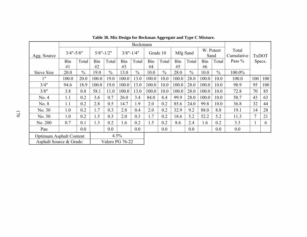
170
Table 38. Mix Design for Beckman Aggregate and Type C Mixture.
Agg. Source
Beckmann Total
Cumulative Pass %
TxDOT Specs.
3/4"-5/8" 5/8"-1/2" 3/8"-1/4" Grade 10 Mfg Sand W. Poteet Sand
Sieve Size
Bin #1
Total Bin #2
Total Bin #3
Total Bin #4
Total Bin #5
Total Bin #6
Total
20.0 % 19.0 % 13.0 % 10.0 % 28.0 % 10.0 % 100.0% 1" 100.0 20.0 100.0 19.0 100.0 13.0 100.0 10.0 100.0 28.0 100.0 10.0 100.0 100 100
3/4" 94.6 18.9 100.0 19.0 100.0 13.0 100.0 10.0 100.0 28.0 100.0 10.0 98.9 95 1003/8" 3.8 0.8 58.1 11.0 100.0 13.0 100.0 10.0 100.0 28.0 100.0 10.0 72.8 70 85
No. 4 1.1 0.2 3.6 0.7 26.0 3.4 84.0 8.4 99.9 28.0 100.0 10.0 50.7 43 63 No. 8 1.1 0.2 2.8 0.5 14.7 1.9 2.0 0.2 85.6 24.0 99.8 10.0 36.8 32 44 No. 30 1.0 0.2 1.7 0.3 2.8 0.4 2.0 0.2 32.9 9.2 88.0 8.8 19.1 14 28 No. 50 1.0 0.2 1.5 0.3 2.0 0.3 1.7 0.2 18.6 5.2 52.2 5.2 11.3 7 21 No. 200 0.7 0.1 1.3 0.2 1.6 0.2 1.5 0.2 8.6 2.4 1.6 0.2 3.3 1 6
Pan 0.0 0.0 0.0 0.0 0.0 0.0 0.0 Optimum Asphalt Content 4.5% Asphalt Source & Grade: Valero PG 76-22

171
Table 39. Mix Design for 50 Percent Brownlee + 50 Percent Beckman Aggregate and Type C Mixture.
Agg. Source
Delta Materials Beckmann Total
Cumulative Pass %
TxDOTSpecs.
Type C Type D 3/4"-5/8" 3/8"-1/4" Mfg Sand Washed Poteet Sand
Sieve Size
Bin #1 Total Bin
#2 Total Bin #3 Total Bin
#4 Total Bin #5 Total Bin
#6 Total
9.0 % 19.0 % 8.0 % 22.0 % 27.0 % 15.0 % 100.0% 7/8" 100.0 9.0 100.0 19.0 100.0 8.0 100.0 22.0 100.0 27.0 100.0 15.0 100.0 98 1005/8" 96.6 8.7 100.0 19.0 89.2 7.1 100.0 22.0 100.0 27.0 100.0 15.0 98.8 95 1003/8" 3.8 0.3 70.9 13.5 3.8 0.3 100.0 22.0 100.0 27.0 100.0 15.0 78.1 70 85
No. 4 1.5 0.1 16.3 3.1 1.1 0.1 26.0 5.7 99.9 27.0 100.0 15.0 51.0 43 63 No. 10 1.0 0.1 4.0 0.8 1.0 0.1 3.4 0.7 70.9 19.1 99.6 14.9 35.7 30 40 No. 40 0.7 0.1 2.3 0.4 1.0 0.1 2.1 0.5 25.0 6.8 69.2 10.4 18.3 10 25 No. 80 0.6 0.1 1.8 0.3 0.9 0.1 1.9 0.4 13.1 3.5 14.4 2.2 6.6 3 13 No. 200 0.4 0.0 1.1 0.2 0.7 0.1 1.6 0.4 8.6 2.3 1.6 0.2 3.2 1 6
Pan 0.0 0.0 0.0 0.0 0.0 0.0 0.0 Optimum Asphalt Content 4.7% Asphalt Source & Grade: Valero PG 76-22

172
Table 40. Mix Design for Brownlee Aggregate and Type C Mixture.
Agg. Source
Delta Materials Capitol-GT RTI-N TXI Total
Cumulative Pass %
TxDOTSpecs.
Delta C D-Rock F-Rock Dry Screenings Washed Screening Field Sand
Sieve Size
Bin #1 Total Bin
#2 Total Bin #3 Total Bin
#4 Total Bin #5 Total Bin
#6 Total
24.0 % 27.0 % 5.0 % 9.0 % 23.0 % 12.0 % 100.0% 7/8" 100.0 24.0 100.0 27.0 100.0 5.0 100.0 9.0 100.0 23.0 100.0 12.0 100.0 98 1005/8" 95.6 22.9 100.0 27.0 100.0 5.0 100.0 9.0 100.0 23.0 100.0 12.0 98.9 95 1003/8" 3.8 0.9 88.4 23.9 100.0 5.0 100.0 9.0 100.0 23.0 100.0 12.0 73.8 70 85 #4 3.7 0.9 37.6 10.2 73.2 3.7 99.8 9.0 98.7 22.7 100.0 12.0 58.4 43 63 #10 3.6 0.9 4.4 1.2 10.2 0.5 80.7 7.3 46.6 10.7 100.0 12.0 32.5 30 40 #40 3.5 0.8 0.7 0.2 2.2 0.1 49.6 4.5 17.4 4.0 87.2 10.5 20.1 10 25 #80 3.4 0.8 0.6 0.2 1.7 0.1 36.4 3.3 11.0 2.5 28.7 3.4 10.3 3 13 #200 3.3 0.8 0.4 0.1 1.1 0.1 27.6 2.5 4.7 1.1 6.0 0.7 5.2 1 6 Pan 0.0 0.0 0.0 0.0 0.0 0.0 0.0
Optimum Asphalt Content 4.50% Asphalt Source & Grade: Fina or Valero PG 76-22

173
Table 41. Mix Design for Fordyce Aggregate and Type C Mixture.
Agg. Source
Fordyce C Fordyce D/F Fordyce Man Sand
Cl Mt Limestone Screening
Austin White Total
CumulativePass %
TxDOTSpecs.
1323505 1323505 1323505 1504605 Lime
Sieve Size
Bin #1 Total Bin
#2 Total Bin #3 Total Bin
#4 Total Bin #5 Total
18.0 % 57.0 % 10.0 % 14.0 % 1.0 % 1" 100.0 18.0 100.0 57.0 100.0 10.0 100.0 14.0 100.0 1.0 100.0
3/4" 100.0 18.0 100.0 57.0 100.0 10.0 100.0 14.0 100.0 1.0 100.0 98 1001/2" 70.0 12.6 100.0 57.0 100.0 10.0 100.0 14.0 100.0 1.0 94.6 90 1003/8" 10.0 1.8 95.0 54.2 100.0 10.0 100.0 14.0 100.0 1.0 81.0 70 95
No. 4 5.0 0.9 50.0 28.5 100.0 10.0 100.0 14.0 100.0 1.0 54.4 43 63 No. 8 3.0 0.5 15.0 8.6 99.0 9.9 92.0 12.9 100.0 1.0 32.9 32 44 No. 30 2.0 0.4 4.0 2.3 49.0 4.9 54.0 7.6 100.0 1.0 16.2 14 28 No. 50 1.5 0.3 3.0 1.7 23.0 2.3 41.0 5.7 100.0 1.0 11.0 7 21 No. 200 0.5 0.1 1.0 0.6 3.0 0.3 25.0 3.5 100.0 1.0 5.5 1 6
Pan Optimum Asphalt Content 4.50% Asphalt Source &Grade:
Eagle PG 76-22
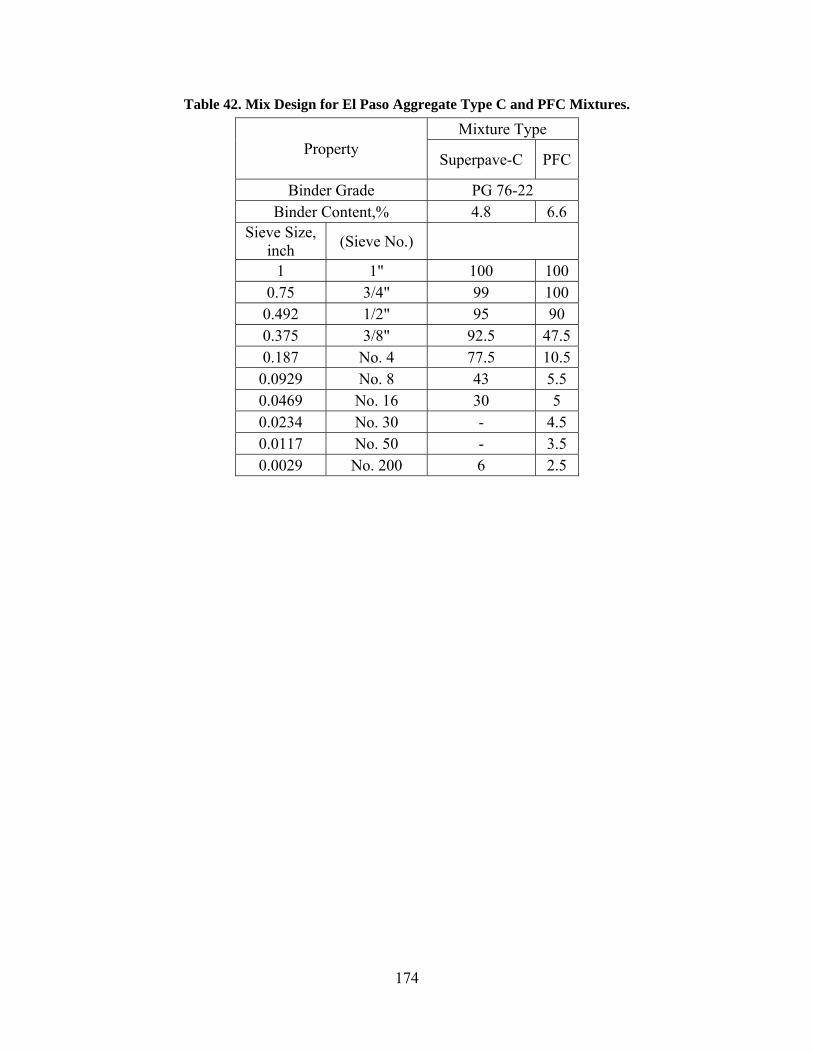
174
Table 42. Mix Design for El Paso Aggregate Type C and PFC Mixtures.
Property Mixture Type
Superpave-C PFC
Binder Grade PG 76-22 Binder Content,% 4.8 6.6
Sieve Size, inch (Sieve No.)
1 1" 100 100 0.75 3/4" 99 100 0.492 1/2" 95 90 0.375 3/8" 92.5 47.5 0.187 No. 4 77.5 10.5 0.0929 No. 8 43 5.5 0.0469 No. 16 30 5 0.0234 No. 30 - 4.5 0.0117 No. 50 - 3.5 0.0029 No. 200 6 2.5
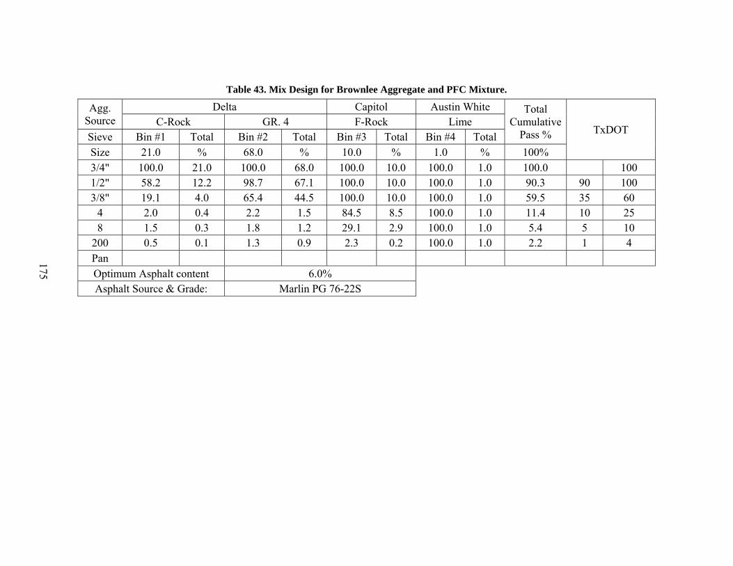
175
Table 43. Mix Design for Brownlee Aggregate and PFC Mixture.
Agg. Source
Delta Capitol Austin White Total Cumulative
Pass % TxDOT C-Rock GR. 4 F-Rock Lime
Sieve Bin #1 Total Bin #2 Total Bin #3 Total Bin #4 Total Size 21.0 % 68.0 % 10.0 % 1.0 % 100% 3/4" 100.0 21.0 100.0 68.0 100.0 10.0 100.0 1.0 100.0 100 1/2" 58.2 12.2 98.7 67.1 100.0 10.0 100.0 1.0 90.3 90 100 3/8" 19.1 4.0 65.4 44.5 100.0 10.0 100.0 1.0 59.5 35 60
4 2.0 0.4 2.2 1.5 84.5 8.5 100.0 1.0 11.4 10 25 8 1.5 0.3 1.8 1.2 29.1 2.9 100.0 1.0 5.4 5 10
200 0.5 0.1 1.3 0.9 2.3 0.2 100.0 1.0 2.2 1 4 Pan Optimum Asphalt content 6.0% Asphalt Source & Grade: Marlin PG 76-22S
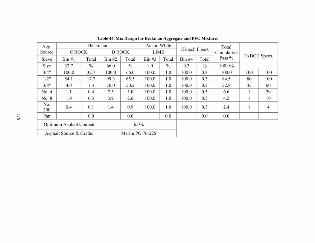
176
Table 44. Mix Design for Beckman Aggregate and PFC Mixture.
Agg. Source
Beckmann Austin White Hi-tech Fibers Total
Cumulative Pass % TxDOT Specs.
C ROCK D ROCK LIME Sieve Bin #1 Total Bin #2 Total Bin #3 Total Bin #4 Total Size 32.7 % 66.0 % 1.0 % 0.3 % 100.0% 3/4" 100.0 32.7 100.0 66.0 100.0 1.0 100.0 0.3 100.0 100 100 1/2" 54.1 17.7 99.3 65.5 100.0 1.0 100.0 0.3 84.5 80 100 3/8" 4.0 1.3 76.0 50.2 100.0 1.0 100.0 0.3 52.8 35 60
No. 4 1.1 0.4 7.5 5.0 100.0 1.0 100.0 0.3 6.6 1 20 No. 8 1.0 0.3 3.9 2.6 100.0 1.0 100.0 0.3 4.2 1 10 No. 200 0.4 0.1 1.4 0.9 100.0 1.0 100.0 0.3 2.4 1 4
Pan 0.0 0.0 0.0 0.0 0.0
Optimum Asphalt Content 6.0%
Asphalt Source & Grade: Marlin PG 76-22S
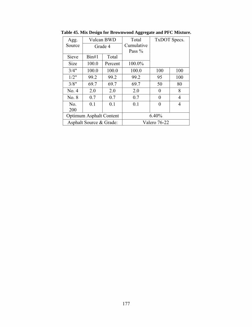
177
Table 45. Mix Design for Brownwood Aggregate and PFC Mixture. Agg.
Source Vulcan BWD Total
Cumulative Pass %
TxDOT Specs. Grade 4
Sieve Bin#1 Total Size 100.0 Percent 100.0% 3/4" 100.0 100.0 100.0 100 100 1/2" 99.2 99.2 99.2 95 100 3/8" 69.7 69.7 69.7 50 80
No. 4 2.0 2.0 2.0 0 8 No. 8 0.7 0.7 0.7 0 4 No. 200
0.1 0.1 0.1 0 4
Optimum Asphalt Content 6.40% Asphalt Source & Grade: Valero 76-22

178
Table 46. Mix Design for Beckman Aggregate and Type D Mixture.
Agg. Source
Beckmann Total
Cumulative Pass %
TxDOT Specs.
1/2" - 3/8" 3/8" - 1/4" Grade 10 Mfg Sand/LSF W. Poteet Sand
Sieve Size
Bin #1
Total Bin #2
Total Bin #3
Total Bin #4
Total Bin #5
Total
9 % 34 % 20 % 22 % 15 % 100%
3/4" 100 9 100 34 100 20 100 22 100 15 100 100 100 1/2" 100 9 100 34 100 20 100 22 100 15 100 98 100 3/8" 66 5.94 100 34 100 20 100 22 100 15 96.94 85 100
No. 4 4.7 0.423 26 8.84 84 16.8 99.9 21.978 100 15 63.041 50 70 No. 8 3.8 0.342 14.7 4.998 2 0.4 85.6 18.832 99.8 14.97 39.542 35 46 No. 30 2.7 0.243 2.8 0.952 2 0.4 32.9 7.238 88 13.2 22.033 15 29 No. 50 2.4 0.216 2 0.68 1.7 0.34 18.6 4.092 52.2 7.83 13.158 7 20 No. 200 2.1 0.189 1.6 0.544 1.5 0.3 8.6 1.892 1.6 0.24 3.165 2 7
Pan 0 0 0 0 0 0 Optimum Asphalt Content 4.7 Asphalt Source & Grade: Valero PG 64-22

179
Table 47. Mix Design for Brownlee Aggregate and Type D Mixture.
Agg. Source
Delta Capitol-GT Brownlee RTI-N TXI Total
Cumulative Pass % TxDOT
Specs.
D-Rock F-Rock Grade #4 Dry Screenings
Washed Screening Field Sand
Sieve Size
Bin #1 Total Bin
#2 Total Bin #3 Total Bin
#4 Total Bin #5 Total Bin
#6 Total
50.0 % 10.0 % 7.0 % 0.0 % 21.0 % 12.0 % 100.0
7/8" 100.0 50.0 100.0 10.0 100.0 7.0 100.0 0.0 100.0 21.0 100.0 12.0 100.0 100 100 5/8" 100.0 50.0 100.0 10.0 100.0 7.0 100.0 0.0 100.0 21.0 100.0 12.0 100.0 98 100 3/8" 79.9 40.0 100.0 10.0 60.0 4.2 100.0 0.0 100.0 21.0 100.0 12.0 87.2 85 100
No. 4 40.3 20.1 77.9 7.8 10.4 0.7 97.5 0.0 99.6 20.9 100.0 12.0 61.6 50 70 No. 10 14.7 7.3 10.2 1.0 0.7 0.1 74.5 0.0 84.0 17.6 99.3 11.9 38.0 35 46 No. 40 9.4 4.7 2.7 0.3 0.6 0.0 41.9 0.0 32.0 6.7 84.4 10.1 21.8 15 29 No. 80 8.5 4.2 2.0 0.2 0.5 0.0 34.6 0.0 11.4 2.4 15.9 1.9 8.8 7 20 No. 200 6.9 3.4 1.5 0.2 0.5 0.0 26.7 0.0 3.1 0.7 0.7 0.1 4.4 2 7 Optimum Asphalt Content 5.3%
Asphalt Source & Grade: Valero PG 76-22

180
Table 48. Mix Design for 50 Percent Beckman and 50 Percent Brownlee and Type D Mixture.
Agg. Source
Delta Materials Beckmann Beckmann Total
Cumulative Pass % TxDOT
Specs.
Brownlee Type D 3/8"-1/4" Mfg Sand W. Poteet Sand Sieved Mfg Sand
Sieve Size
Bin #1 Total Bin
#2 Total Bin #3 Total Bin #4 Total Bin #5 Total
20.0 % 31.0 % 31.0 % 11.0 % 7.0 % 100%
7/8" 100.0 20.0 100.0 31.0 100.0 31.0 100.0 11.0 100.0 7.0 100.0 100 100 5/8" 100.0 20.0 100.0 31.0 100.0 31.0 100.0 11.0 100.0 7.0 100.0 98 100 3/8" 70.9 14.2 100.0 31.0 100.0 31.0 100.0 11.0 100.0 7.0 94.2 85 100
No. 4 16.3 3.3 26.0 8.1 99.9 31.0 100.0 11.0 100.0 7.0 60.3 50 70 No. 10 4.0 0.8 3.4 1.1 70.9 22.0 99.6 11.0 100.0 7.0 41.8 35 46 No. 40 2.3 0.5 2.1 0.7 25.0 7.8 69.2 7.6 100.0 7.0 23.5 15 29 No. 80 1.8 0.4 1.9 0.6 13.1 4.1 14.4 1.6 100.0 7.0 13.6 7 20 No. 200 1.1 0.2 1.6 0.5 8.6 2.7 1.6 0.2 0.0 0.0 3.6 2 7 Optimum Asphalt Content 5.3% Asphalt Source & Grade: Valero PG 76-22
181
APPENDIX B – TEXTURE AND ANGULARITY MEASUREMENTS BY AIMS FOR DIFFERENT AGGREGATES

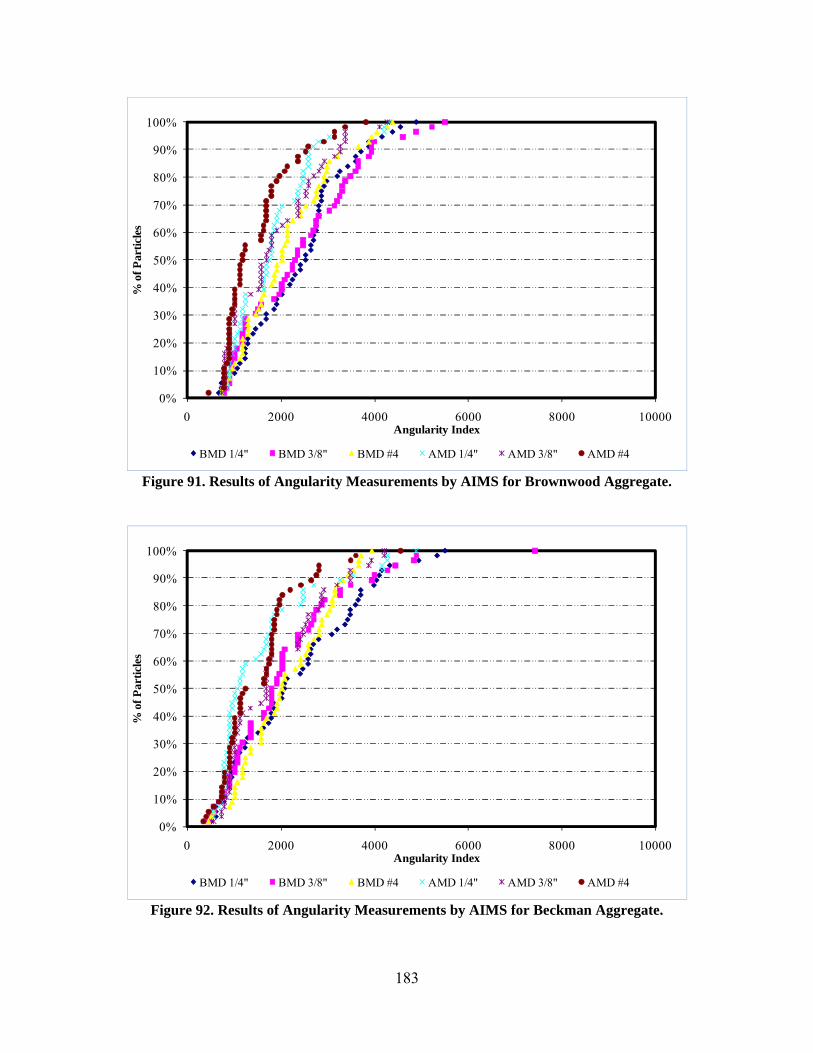
183
Figure 91. Results of Angularity Measurements by AIMS for Brownwood Aggregate.
Figure 92. Results of Angularity Measurements by AIMS for Beckman Aggregate.
0%
10%
20%
30%
40%
50%
60%
70%
80%
90%
100%
0 2000 4000 6000 8000 10000
% o
f Par
ticle
s
Angularity Index
BMD 1/4" BMD 3/8" BMD #4 AMD 1/4" AMD 3/8" AMD #4
0%
10%
20%
30%
40%
50%
60%
70%
80%
90%
100%
0 2000 4000 6000 8000 10000
% o
f Par
ticle
s
Angularity Index
BMD 1/4" BMD 3/8" BMD #4 AMD 1/4" AMD 3/8" AMD #4
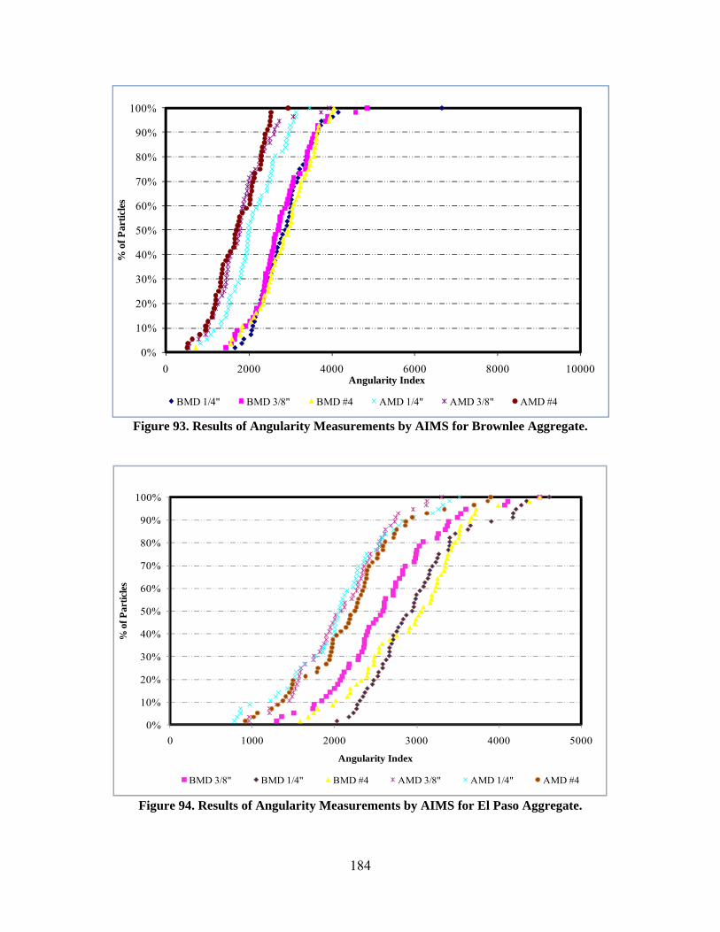
184
Figure 93. Results of Angularity Measurements by AIMS for Brownlee Aggregate.
Figure 94. Results of Angularity Measurements by AIMS for El Paso Aggregate.
0%
10%
20%
30%
40%
50%
60%
70%
80%
90%
100%
0 2000 4000 6000 8000 10000
% o
f Par
ticle
s
Angularity Index
BMD 1/4" BMD 3/8" BMD #4 AMD 1/4" AMD 3/8" AMD #4
0%
10%
20%
30%
40%
50%
60%
70%
80%
90%
100%
0 1000 2000 3000 4000 5000
% o
f Par
ticle
s
Angularity Index
BMD 3/8" BMD 1/4" BMD #4 AMD 3/8" AMD 1/4" AMD #4
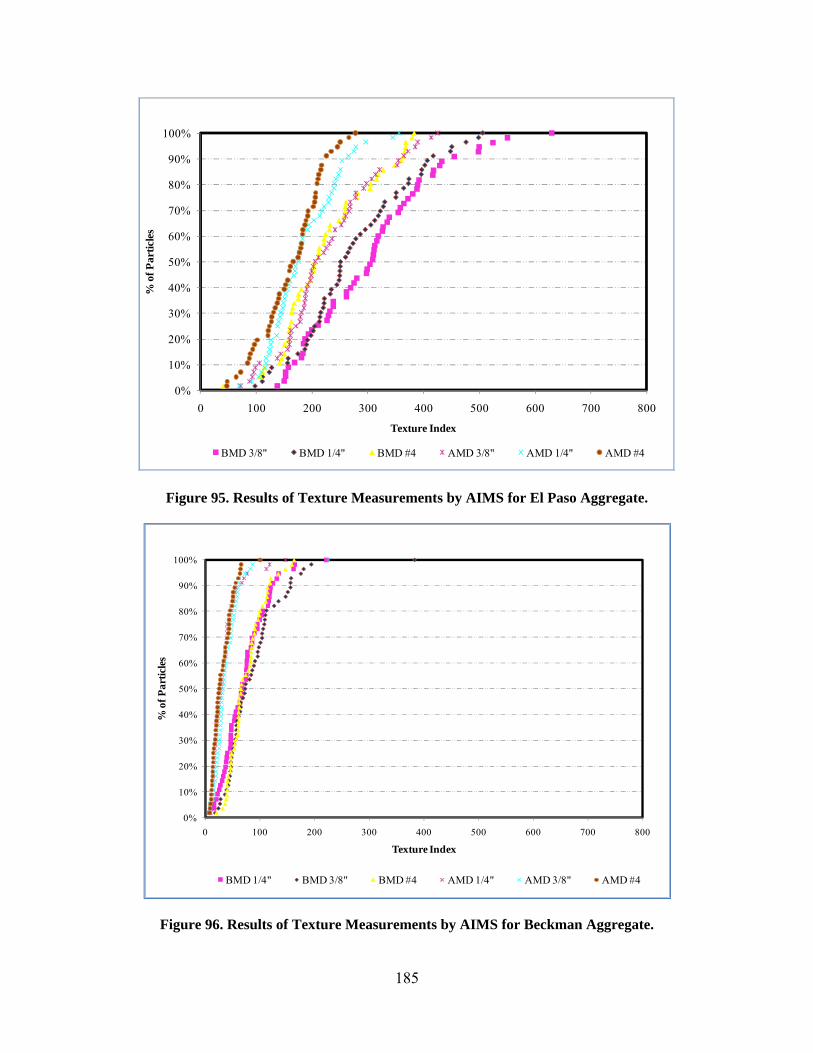
185
Figure 95. Results of Texture Measurements by AIMS for El Paso Aggregate.
Figure 96. Results of Texture Measurements by AIMS for Beckman Aggregate.
0%
10%
20%
30%
40%
50%
60%
70%
80%
90%
100%
0 100 200 300 400 500 600 700 800
% o
f Par
ticle
s
Texture Index
BMD 3/8" BMD 1/4" BMD #4 AMD 3/8" AMD 1/4" AMD #4
0%
10%
20%
30%
40%
50%
60%
70%
80%
90%
100%
0 100 200 300 400 500 600 700 800
% o
f Par
ticle
s
Texture Index
BMD 1/4" BMD 3/8" BMD #4 AMD 1/4" AMD 3/8" AMD #4
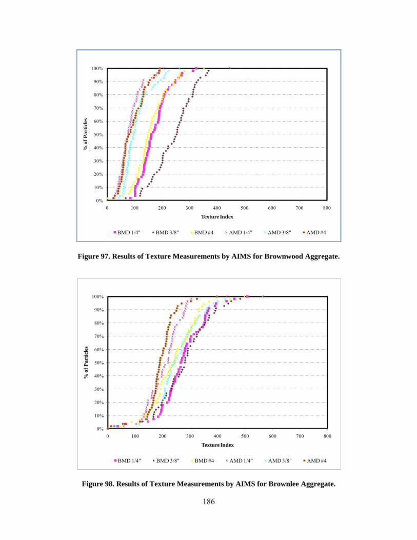
186
Figure 97. Results of Texture Measurements by AIMS for Brownwood Aggregate.
Figure 98. Results of Texture Measurements by AIMS for Brownlee Aggregate.
0%
10%
20%
30%
40%
50%
60%
70%
80%
90%
100%
0 100 200 300 400 500 600 700 800
% o
f Par
ticle
s
Texture Index
BMD 1/4" BMD 3/8" BMD #4 AMD 1/4" AMD 3/8" AMD #4
0%
10%
20%
30%
40%
50%
60%
70%
80%
90%
100%
0 100 200 300 400 500 600 700 800
% o
f Par
ticle
s
Texture Index
BMD 1/4" BMD 3/8" BMD #4 AMD 1/4" AMD 3/8" AMD #4

187
APPENDIX C – PLOTS OF TERMINAL AND RATE OF CHANGE VALUES FOR F60 AND DF20 FOR DIFFERENT AGGREGATE AND
MIXES

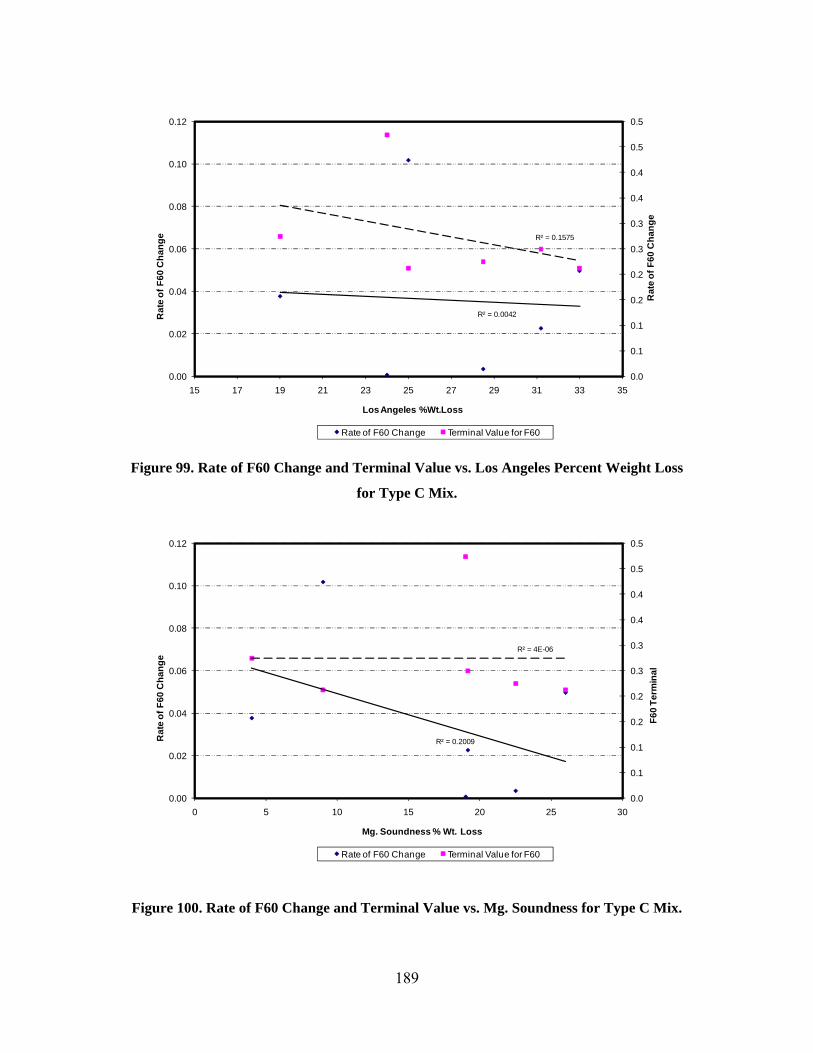
189
Figure 99. Rate of F60 Change and Terminal Value vs. Los Angeles Percent Weight Loss
for Type C Mix.
Figure 100. Rate of F60 Change and Terminal Value vs. Mg. Soundness for Type C Mix.
R² = 0.0042
R² = 0.1575
0.0
0.1
0.1
0.2
0.2
0.3
0.3
0.4
0.4
0.5
0.5
0.00
0.02
0.04
0.06
0.08
0.10
0.12
15 17 19 21 23 25 27 29 31 33 35
Rat
e of
F60
Cha
nge
Rat
e of
F60
Cha
nge
Los Angeles %Wt.Loss
Rate of F60 Change Terminal Value for F60
R² = 0.2009
R² = 4E-06
0.0
0.1
0.1
0.2
0.2
0.3
0.3
0.4
0.4
0.5
0.5
0.00
0.02
0.04
0.06
0.08
0.10
0.12
0 5 10 15 20 25 30
F60
Term
inal
Rat
e of
F60
Cha
nge
Mg. Soundness % Wt. Loss
Rate of F60 Change Terminal Value for F60
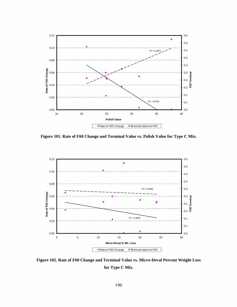
190
Figure 101. Rate of F60 Change and Terminal Value vs. Polish Value for Type C Mix.
Figure 102. Rate of F60 Change and Terminal Value vs. Micro-Deval Percent Weight Loss
for Type C Mix.
R² = 0.6792
R² = 0.6971
0.0
0.1
0.1
0.2
0.2
0.3
0.3
0.4
0.4
0.5
0.5
0.00
0.02
0.04
0.06
0.08
0.10
0.12
15 20 25 30 35 40
F60
Term
inal
Rat
e of
F60
Cha
nge
Polish Value
Rate of F60 Change Terminal Value for F60
R² = 0.0545
R² = 0.0065
0.0
0.1
0.1
0.2
0.2
0.3
0.3
0.4
0.4
0.5
0.5
0.00
0.02
0.04
0.06
0.08
0.10
0.12
0 5 10 15 20 25 30
F60
Term
inal
Rat
e of
F60
Cha
nge
Micro-Deval % Wt. Loss
Rate of F60 Change Terminal Value for F60

191
Figure 103. Rate of F60 Change and Terminal Value vs. Coarse Aggregate Acid Insolubility
for Type C Mix.
Figure 104. Rate of F60 Change and Terminal Value vs. Change in Texture BMD and AMD
for Type C Mix.
R² = 0.2728
R² = 0.3508
0.0
0.1
0.1
0.2
0.2
0.3
0.3
0.4
0.4
0.5
0.5
0.00
0.02
0.04
0.06
0.08
0.10
0.12
0 10 20 30 40 50 60 70 80 90
F60
Term
inal
Rat
e of
F60
Cha
nge
Coarse Aggregate Acid Insolubility
Rate of F60 Change Terminal Value for F60
R² = 0.6429
R² = 0.4361
0.0
0.1
0.1
0.2
0.2
0.3
0.3
0.4
0.4
0.5
0.5
0.00
0.02
0.04
0.06
0.08
0.10
0.12
0.0 0.1 0.2 0.3 0.4 0.5 0.6
F60
Term
inal
Rat
e of
F60
Cha
nge
Change in Texture BMD and AMD
Rate of F60 Change Terminal Value for F60
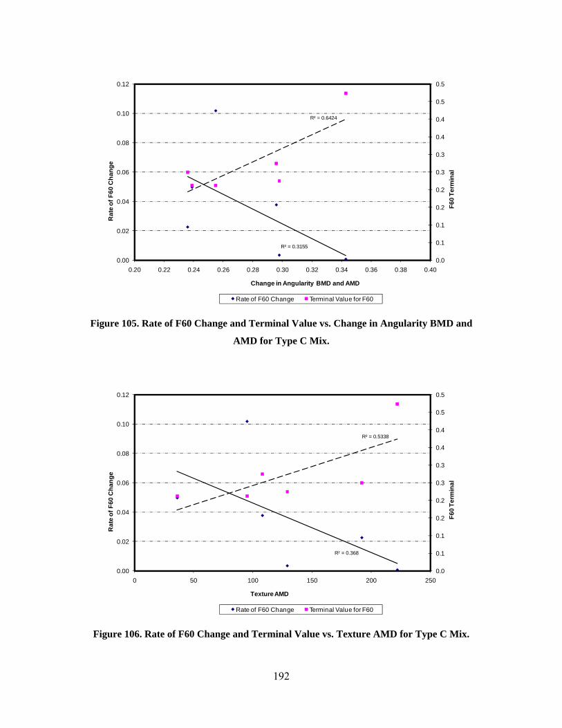
192
Figure 105. Rate of F60 Change and Terminal Value vs. Change in Angularity BMD and
AMD for Type C Mix.
Figure 106. Rate of F60 Change and Terminal Value vs. Texture AMD for Type C Mix.
R² = 0.3155
R² = 0.6424
0.0
0.1
0.1
0.2
0.2
0.3
0.3
0.4
0.4
0.5
0.5
0.00
0.02
0.04
0.06
0.08
0.10
0.12
0.20 0.22 0.24 0.26 0.28 0.30 0.32 0.34 0.36 0.38 0.40
F60
Term
inal
Rat
e of
F60
Cha
nge
Change in Angularity BMD and AMD
Rate of F60 Change Terminal Value for F60
R² = 0.368
R² = 0.5338
0.0
0.1
0.1
0.2
0.2
0.3
0.3
0.4
0.4
0.5
0.5
0.00
0.02
0.04
0.06
0.08
0.10
0.12
0 50 100 150 200 250
F60
Term
inal
Rat
e of
F60
Cha
nge
Texture AMD
Rate of F60 Change Terminal Value for F60
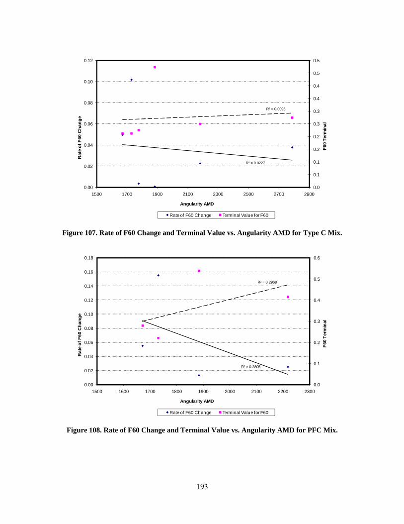
193
Figure 107. Rate of F60 Change and Terminal Value vs. Angularity AMD for Type C Mix.
Figure 108. Rate of F60 Change and Terminal Value vs. Angularity AMD for PFC Mix.
R² = 0.0227
R² = 0.0095
0.0
0.1
0.1
0.2
0.2
0.3
0.3
0.4
0.4
0.5
0.5
0.00
0.02
0.04
0.06
0.08
0.10
0.12
1500 1700 1900 2100 2300 2500 2700 2900
F60
Term
inal
Rat
e of
F60
Cha
nge
Angularity AMD
Rate of F60 Change Terminal Value for F60
R² = 0.2805
R² = 0.2968
0.0
0.1
0.2
0.3
0.4
0.5
0.6
0.00
0.02
0.04
0.06
0.08
0.10
0.12
0.14
0.16
0.18
1500 1600 1700 1800 1900 2000 2100 2200 2300
F60
Term
inal
Rat
e of
F60
Cha
nge
Angularity AMD
Rate of F60 Change Terminal Value for F60
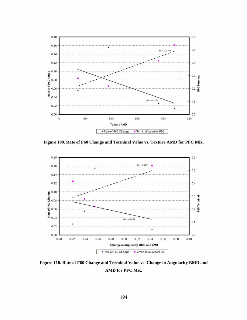
194
Figure 109. Rate of F60 Change and Terminal Value vs. Texture AMD for PFC Mix.
Figure 110. Rate of F60 Change and Terminal Value vs. Change in Angularity BMD and
AMD for PFC Mix.
R² = 0.3173
R² = 0.7703
0.0
0.1
0.2
0.3
0.4
0.5
0.6
0.00
0.02
0.04
0.06
0.08
0.10
0.12
0.14
0.16
0.18
0 50 100 150 200 250
F60
Term
inal
Rat
e of
F60
Cha
nge
Texture AMD
Rate of F60 Change Terminal Value for F60
R² = 0.0788
R² = 0.4202
0.0
0.1
0.2
0.3
0.4
0.5
0.6
0.00
0.02
0.04
0.06
0.08
0.10
0.12
0.14
0.16
0.18
0.20 0.22 0.24 0.26 0.28 0.30 0.32 0.34 0.36 0.38 0.40
F60
Term
inal
Rat
e of
F60
Cha
nge
Change in Angularity BMD and AMD
Rate of F60 Change Terminal Value for F60

195
Figure 111. Rate of F60 Change and Terminal Value vs. Change in Texture BMD and AMD
for PFC Mix.
Figure 112. Rate of F60 Change and Terminal Value vs. Coarse Aggregate Acid Insolubility
for PFC Mix.
R² = 0.5016
R² = 0.9101
0.0
0.1
0.2
0.3
0.4
0.5
0.6
0.00
0.02
0.04
0.06
0.08
0.10
0.12
0.14
0.16
0.18
0.0 0.1 0.2 0.3 0.4 0.5 0.6
F60
Term
inal
Rat
e of
F60
Cha
nge
Change in Texture BMD and AMD
Rate of F60 Change Terminal Value for F60
R² = 0.5391
R² = 0.9691
0.0
0.1
0.2
0.3
0.4
0.5
0.6
0.00
0.02
0.04
0.06
0.08
0.10
0.12
0.14
0.16
0.18
0 10 20 30 40 50 60 70
F60
Term
inal
Rat
e of
F60
Cha
nge
Coarse Aggregate Acid Insolubility
Rate of F60 Change Terminal Value for F60

196
Figure 113. Rate of F60 Change and Terminal Value vs. Micro-Deval Percent Weight Loss
for PFC Mix.
Figure 114. Rate of F60 Change and Terminal Value vs. Polish Value for PFC Mix.
R² = 0.135
R² = 0.002
0.0
0.1
0.2
0.3
0.4
0.5
0.6
0.00
0.02
0.04
0.06
0.08
0.10
0.12
0.14
0.16
0.18
10.0 12.0 14.0 16.0 18.0 20.0 22.0 24.0 26.0 28.0 30.0
F60
Term
inal
Rat
e of
F60
Cha
nge
Micro-Deval % Wt. Loss
Rate of F60 Change Terminal Value for F60
R² = 0.514
R² = 0.8282
0.0
0.1
0.2
0.3
0.4
0.5
0.6
0.00
0.02
0.04
0.06
0.08
0.10
0.12
0.14
0.16
0.18
15 20 25 30 35 40
F60
Term
inal
Rat
e of
F60
Cha
nge
Polish Value
Rate of F60 Change Terminal Value for F60

197
Figure 115. Rate of F60 Change and Terminal Value vs. Mg. Soundness for PFC Mix.
Figure 116. Rate of F60 Change and Terminal Value vs. Los Angeles Percent Weight Loss
PFC Mix.
R² = 0.5331
R² = 0.0811
0.0
0.1
0.2
0.3
0.4
0.5
0.6
0.00
0.02
0.04
0.06
0.08
0.10
0.12
0.14
0.16
0.18
0 5 10 15 20 25 30
F60
Term
inal
Rat
e of
F60
Cha
nge
Mg. Soundness % Wt. Loss
Rate of F60 Change Terminal Value for F60
R² = 0.0876
R² = 0.0596
0.0
0.1
0.2
0.3
0.4
0.5
0.6
0.00
0.02
0.04
0.06
0.08
0.10
0.12
0.14
0.16
0.18
20 22 24 26 28 30 32 34
F60
Term
inal
Rat
e of
F60
Cha
nge
Los Angeles %Wt.Loss
Rate of F60 Change Terminal Value for F60

198
Figure 117. Rate of DF20 Change and Terminal Value vs. Los Angeles Percent Weight Loss
for Type C Mix.
Figure 118. Rate of DF20 Change and Terminal Value vs. Mg Soundness for Type C Mix.
R² = 0.0053
R² = 0.1384
0.0
0.1
0.2
0.3
0.4
0.5
0.6
0.7
0.8
0.9
0.00
0.01
0.02
0.03
0.04
0.05
0.06
0.07
0.08
0.09
0.10
15 17 19 21 23 25 27 29 31 33 35
DF 2
0Te
rmin
al
Rat
e of
DF 2
0C
hang
e
Los Angeles % Wt. Loss
Rate of DF20 Change Terminal Value for DF20
R² = 0.0922
R² = 0.0081
0.0
0.1
0.2
0.3
0.4
0.5
0.6
0.7
0.8
0.9
0.00
0.01
0.02
0.03
0.04
0.05
0.06
0.07
0.08
0.09
0.10
0 5 10 15 20 25 30
DF 2
0Te
rmin
al
Rat
e of
DF 2
0C
hang
e
Mg. Soundness % Wt. Loss
Rate of DF20 Change Terminal Value for DF20
Rate of DF20 Change Terminal Value for DF20
Rate of DF20 Change Terminal Value for DF20

199
Figure 119. Rate of DF20 Change and Terminal Value vs. Polish Value for Type C Mix.
Figure 120. Rate of DF20 Change and Terminal Value vs. Micro-Deval Percent Weight Loss
for Type C Mix.
R² = 0.6732
R² = 0.9044
0.0
0.1
0.2
0.3
0.4
0.5
0.6
0.7
0.8
0.9
0.00
0.01
0.02
0.03
0.04
0.05
0.06
0.07
0.08
0.09
0.10
15 20 25 30 35 40
DF 2
0 Te
rmin
al
Rat
e of
DF 2
0C
hang
e
Polish Value
Rate of DF20 Change Terminal Value for DF20
R² = 0.0053
R² = 5E-07
0.0
0.1
0.2
0.3
0.4
0.5
0.6
0.7
0.8
0.9
0.00
0.01
0.02
0.03
0.04
0.05
0.06
0.07
0.08
0.09
0.10
0.0 5.0 10.0 15.0 20.0 25.0 30.0
DF 2
0Te
rmin
al
Rat
e of
DF 2
0C
hang
e
Micro-Deval %Wt. Loss
Rate of DF20 Change Terminal Value for DF20
Rate of DF20 Change Terminal Value for DF20
Rate of DF20 Change Terminal Value for DF20

200
Figure 121. Rate of DF20 Change and Terminal Value vs. Coarse Aggregate Acid
Insolubility for Type C Mix.
Figure 122. Rate of DF20 Change and Terminal Value vs. Change in Texture BMD and
AMD for Type C Mix.
R² = 0.4314
R² = 0.3845
0.0
0.1
0.2
0.3
0.4
0.5
0.6
0.7
0.8
0.9
0.00
0.01
0.02
0.03
0.04
0.05
0.06
0.07
0.08
0.09
0.10
0 10 20 30 40 50 60 70 80 90
DF 2
0Te
rmin
al
Rat
e of
DF 2
0C
hang
e
Coarse Aggregate Acid Insolubility
Rate of DF20 Change Terminal Value for DF20
R² = 0.7318
R² = 0.6928
0.0
0.1
0.2
0.3
0.4
0.5
0.6
0.7
0.8
0.9
0.00
0.01
0.02
0.03
0.04
0.05
0.06
0.07
0.08
0.09
0.10
0.10 0.20 0.30 0.40 0.50 0.60
DF 2
0Te
rmin
al
Rat
e of
DF 2
0C
hang
e
Change in Texture BMD and AMD
Rate of DF20 Change Terminal Value for DF20
Rate of DF20 Change Terminal Value for DF20
Rate of DF20 Change Terminal Value for DF20
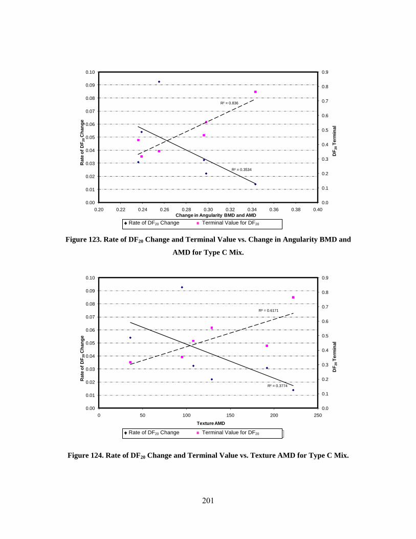
201
Figure 123. Rate of DF20 Change and Terminal Value vs. Change in Angularity BMD and
AMD for Type C Mix.
Figure 124. Rate of DF20 Change and Terminal Value vs. Texture AMD for Type C Mix.
R² = 0.3534
R² = 0.836
0.0
0.1
0.2
0.3
0.4
0.5
0.6
0.7
0.8
0.9
0.00
0.01
0.02
0.03
0.04
0.05
0.06
0.07
0.08
0.09
0.10
0.20 0.22 0.24 0.26 0.28 0.30 0.32 0.34 0.36 0.38 0.40
DF 2
0Te
rmin
al
Rat
e of
DF 2
0C
hang
e
Change in Angularity BMD and AMD
Rate of DF20 Change Terminal Value for DF20
R² = 0.3774
R² = 0.6171
0.0
0.1
0.2
0.3
0.4
0.5
0.6
0.7
0.8
0.9
0.00
0.01
0.02
0.03
0.04
0.05
0.06
0.07
0.08
0.09
0.10
0 50 100 150 200 250
DF 2
0Te
rmin
al
Rat
e of
DF 2
0C
hang
e
Texture AMD
Rate of DF20 Change Terminal Value for DF20
Rate of DF20 Change Terminal Value for DF20
Rate of DF20 Change Terminal Value for DF20
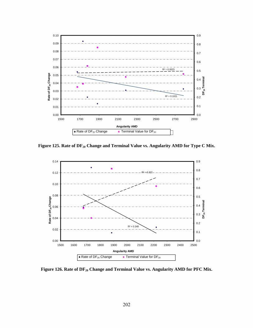
202
Figure 125. Rate of DF20 Change and Terminal Value vs. Angularity AMD for Type C Mix.
Figure 126. Rate of DF20 Change and Terminal Value vs. Angularity AMD for PFC Mix.
R² = 0.1021
R² = 0.0023
0.0
0.1
0.2
0.3
0.4
0.5
0.6
0.7
0.8
0.9
0.00
0.01
0.02
0.03
0.04
0.05
0.06
0.07
0.08
0.09
0.10
1500 1700 1900 2100 2300 2500 2700 2900
DF 2
0Te
rmin
al
Rat
e of
DF 2
0C
hang
e
Angularity AMD
Rate of DF20 Change Terminal Value for DF20
R² = 0.349
R² = 0.322
0.0
0.1
0.2
0.3
0.4
0.5
0.6
0.7
0.8
0.9
0.00
0.02
0.04
0.06
0.08
0.10
0.12
0.14
1500 1600 1700 1800 1900 2000 2100 2200 2300 2400 2500
DF 2
0Te
rmin
al
Rat
e of
DF 2
0 C
hang
e
Angularity AMD
Rate of DF20 Change Terminal Value for DF20
Rate of DF20 Change Terminal Value for DF20
Rate of DF20 Change Terminal Value for DF20

203
Figure 127. Rate of DF20 Change and Terminal Value vs. Texture AMD for PFC Mix.
Figure 128. Rate of DF20 Change and Terminal Value vs. Change in Angularity BMD and
AMD for PFC Mix.
R² = 0.4204
R² = 0.7692
0.0
0.1
0.2
0.3
0.4
0.5
0.6
0.7
0.8
0.9
0.00
0.02
0.04
0.06
0.08
0.10
0.12
0.14
0 50 100 150 200 250
DF 2
0Te
rmin
al
Rat
e of
DF 2
0 C
hang
e
Texture AMD
Rate of DF20 Change Terminal Value for DF20
R² = 0.0994
R² = 0.386
0.0
0.1
0.2
0.3
0.4
0.5
0.6
0.7
0.8
0.9
0.00
0.02
0.04
0.06
0.08
0.10
0.12
0.14
0.20 0.22 0.24 0.26 0.28 0.30 0.32 0.34 0.36 0.38 0.40
DF 2
0Te
rmin
al
Rat
e of
DF 2
0 C
hang
e
Change in Angularity BMD and AMD
Rate of DF20 Change Terminal Value for DF20
Rate of DF20 Change Terminal Value for DF20
Rate of DF20 Change Terminal Value for DF20
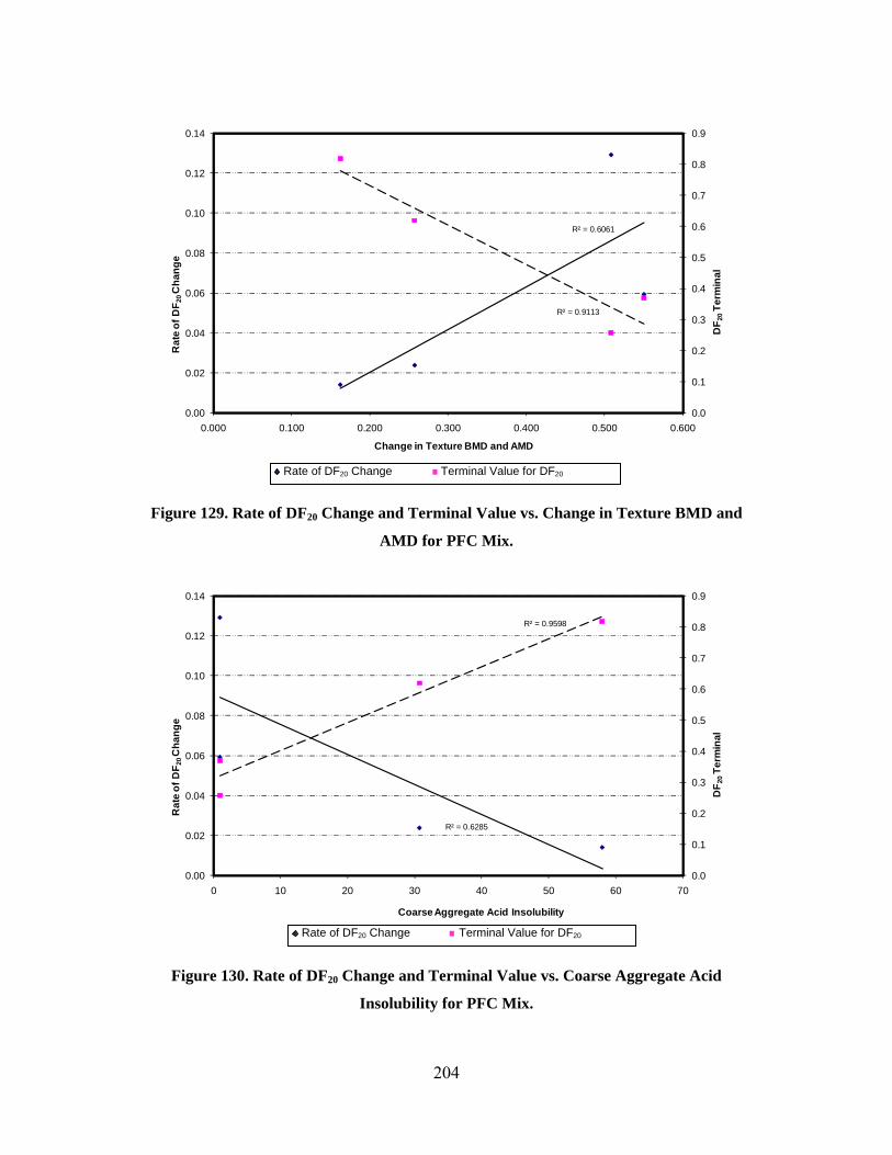
204
Figure 129. Rate of DF20 Change and Terminal Value vs. Change in Texture BMD and
AMD for PFC Mix.
Figure 130. Rate of DF20 Change and Terminal Value vs. Coarse Aggregate Acid
Insolubility for PFC Mix.
R² = 0.6061
R² = 0.9113
0.0
0.1
0.2
0.3
0.4
0.5
0.6
0.7
0.8
0.9
0.00
0.02
0.04
0.06
0.08
0.10
0.12
0.14
0.000 0.100 0.200 0.300 0.400 0.500 0.600
DF 2
0Te
rmin
al
Rat
e of
DF 2
0 C
hang
e
Change in Texture BMD and AMD
Rate of DF20 Change Terminal Value for DF20
R² = 0.6285
R² = 0.9598
0.0
0.1
0.2
0.3
0.4
0.5
0.6
0.7
0.8
0.9
0.00
0.02
0.04
0.06
0.08
0.10
0.12
0.14
0 10 20 30 40 50 60 70
DF 2
0Te
rmin
al
Rat
e of
DF 2
0 C
hang
e
Coarse Aggregate Acid Insolubility
Rate of DF20 Change Terminal Value for DF20
Rate of DF20 Change Terminal Value for DF20
Rate of DF20 Change Terminal Value for DF20

205
Figure 131. Rate of DF20 Change and Terminal Value vs. Micro-Deval Percent Weight Loss
for PFC Mix.
Figure 132. Rate of DF20 Change and Terminal Value vs. Polish Value for PFC Mix.
R² = 0.0716
R² = 0.0017
0.0
0.1
0.2
0.3
0.4
0.5
0.6
0.7
0.8
0.9
0.00
0.02
0.04
0.06
0.08
0.10
0.12
0.14
10 12 14 16 18 20 22 24 26 28 30
DF 2
0Te
rmin
al
Rat
e of
DF 2
0 C
hang
e
Micro-Deval % Wt. Loss
Rate of DF20 Change Terminal Value for DF20
R² = 0.5497
R² = 0.8057
0.0
0.1
0.2
0.3
0.4
0.5
0.6
0.7
0.8
0.9
0.00
0.02
0.04
0.06
0.08
0.10
0.12
0.14
15 20 25 30 35 40
DF 2
0Te
rmin
al
Rat
e of
DF 2
0 C
hang
e
Polish Value
Rate of DF20 Change Terminal Value for DF20
Rate of DF20 Change Terminal Value for DF20
Rate of DF20 Change Terminal Value for DF20

206
Figure 133. Rate of DF20 Change and Terminal Value vs. Mg. Soundness for PFC Mix.
Figure 134. Rate of DF20 Change and Terminal Value vs. Los Angeles Percent Weight Loss
for PFC Mix.
R² = 0.4259
R² = 0.0906
0.0
0.1
0.2
0.3
0.4
0.5
0.6
0.7
0.8
0.9
0.00
0.02
0.04
0.06
0.08
0.10
0.12
0.14
0 5 10 15 20 25 30
DF 2
0Te
rmin
al
Rat
e of
DF 2
0 C
hang
e
Mg. Soundness % Wt. Loss
Rate of DF20 Change Terminal Value for DF20
R² = 0.0515
R² = 0.0455
0.0
0.1
0.2
0.3
0.4
0.5
0.6
0.7
0.8
0.9
0.00
0.02
0.04
0.06
0.08
0.10
0.12
0.14
15 17 19 21 23 25 27 29 31 33 35
DF 2
0Te
rmin
al
Rat
e of
DF 2
0C
hang
e
Los Angeles % Wt .Loss
Rate of DF20 Change Terminal Value for DF20
Rate of DF20 Change Terminal Value for DF20
Rate of DF20 Change Terminal Value for DF20

207
Figure 135. Rate of F60 Change and Terminal Value vs. Angularity AMD
without Brownlee.
Figure 136. Rate of F60 Change and Terminal Value vs. Change in Texture BMD and AMD
without Brownlee.
R² = 0.0227
R² = 0.9661
0.0
0.1
0.1
0.2
0.2
0.3
0.3
0.00
0.02
0.04
0.06
0.08
0.10
0.12
1500 1700 1900 2100 2300 2500 2700 2900
F60
Term
inal
Rat
e of
F60
Cha
nge
Angularity AMD
Rate of F60 Change Terminal Value for F60
R² = 0.6429
R² = 0.5934
0.0
0.1
0.1
0.2
0.2
0.3
0.3
0.00
0.02
0.04
0.06
0.08
0.10
0.12
0.0 0.1 0.2 0.3 0.4 0.5 0.6
F60
Term
inal
Rat
e of
F60
Cha
nge
Change in Texture BMD and AMD
Rate of F60 Change Terminal Value for F60
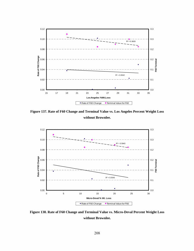
208
Figure 137. Rate of F60 Change and Terminal Value vs. Los Angeles Percent Weight Loss
without Brownlee.
Figure 138. Rate of F60 Change and Terminal Value vs. Micro-Deval Percent Weight Loss
without Brownlee.
R² = 0.0042
R² = 0.3633
0.0
0.1
0.1
0.2
0.2
0.3
0.3
0.00
0.02
0.04
0.06
0.08
0.10
0.12
15 17 19 21 23 25 27 29 31 33 35
F60
Term
inal
Rat
e of
F60
Cha
nge
Los Angeles %Wt.Loss
Rate of F60 Change Terminal Value for F60
R² = 0.0545
R² = 0.5943
0.0
0.1
0.1
0.2
0.2
0.3
0.3
0.00
0.02
0.04
0.06
0.08
0.10
0.12
0 5 10 15 20 25 30
F60
Term
inal
Rat
e of
F60
Cha
nge
Micro-Deval % Wt. Loss
Rate of F60 Change Terminal Value for F60

209
Figure 139. Rate of F60 Change and Terminal Value vs. Coarse Aggregate Acid Insolubility
without Brownlee.
Figure 140. Rate of F60 Change and Terminal Value vs. Mg Soundness without Brownlee.
R² = 0.2728
R² = 0.8343
0.0
0.1
0.1
0.2
0.2
0.3
0.3
0.00
0.02
0.04
0.06
0.08
0.10
0.12
0 10 20 30 40 50 60 70 80 90
F60
Term
inal
Rat
e of
F60
Cha
nge
Coarse Aggregate Acid Insolubility
Rate of F60 Change Terminal Value for F60
R² = 0.2009
R² = 0.3147
0.0
0.1
0.1
0.2
0.2
0.3
0.3
0.00
0.02
0.04
0.06
0.08
0.10
0.12
0 5 10 15 20 25 30
F60
Term
inal
Rat
e of
F60
Cha
nge
Mg. Soundness % Wt. Loss
Rate of F60 Change Terminal Value for F60