öMmföäflsäafaäsflassflassflas ffffffffffffffffffffffffffffffffff

Discussion Papers

Predicting Bear and Bull Stock Markets with Dynamic Binary Time Series Models

Henri Nyberg University of Helsinki

Discussion Paper No. 355 October 2012

ISSN 1795-0562

HECER – Helsinki Center of Economic Research, P.O. Box 17 (Arkadiankatu 7), FI-00014 University of Helsinki, FINLAND, Tel +358-9-191-28780, Fax +358-9-191-28781, E-mail info-hecer@helsinki.fi, Internet www.hecer.fi

brought to you by COREView metadata, citation and similar papers at core.ac.uk

provided by Helsingin yliopiston digitaalinen arkisto

HECER Discussion Paper No. 355

Predicting Bear and Bull Stock Markets with Dynamic Binary Time Series Models* Abstract Despite the voluminous empirical research on the potential predictability of stock returns, very little attention has been paid on the predictability of bear and bull stock markets. In this study, the aim is to predict the U.S. bear and bull stock markets with dynamic binary time series models. Based on the results of monthly U.S. data set, the bear and bull markets are predictable in and out of sample. In particular, substantial additional predictive power can be obtained by allowing for dynamic structures in the employed binary response model. Probability forecasts of the state of the stock market can also be utilized to obtain optimal asset allocation decisions between stocks and bonds. It turns out that the dynamic probit models yield much higher portfolio returns compared with the buy-and-hold trading strategy in a small-scale market timing experiment. JEL Classification: C25, C53, G11, G17 Keywords: Bear markets, turning points, probit model, asset allocation, forecasts. Henri Nyberg Department of Political and Economic Studies University of Helsinki P.O. Box 17 FI-00014 University of Helsinki FINLAND e-mail: henri.nyberg@helsinki.fi * The financial support from the Academy of Finland, the OP-Pohjola Group Research Foundation and the Yrjö Jahnsson Foundation is gratefully acknowledged. Part of this research is done during the research visit at the Faculty of Economics of the University of Cambridge (September 2011 – May 2012).

1 Introduction

A great deal of econometric research has been devoted to examine the behavior

and potential predictability of stock prices. The main objective in the literature

has been to predict the overall return. In contrast to the principles of the efficient

market hypothesis, various authors have suggested that there is some degree of

out-of-sample predictability in the stock returns (see, e.g., Rapach, Wohar and

Rangvid, 2005; Ang and Bekaert, 2007; Campbell and Thompson, 2008, and the

references therein). Returns exhibit various typical features, such as volatility clus-

tering and dependence on the future investment opportunities, which can be used

to predict the behavior of the stock market and potentially be utilized in market

timing decisions in order to earn higher returns than, for example, obtained with

a passive buy-and-hold trading strategy.

Despite the large amount of previous research on stock return predictability

much less attention has been paid on the extensive periods of time when stock

returns are rising or falling. These periods are often referred to as bull and bear

markets, respectively. In this study, the main goal is to predict the state of the

stock market (i.e. bear and bull markets) with dynamic binary time series models

proposed in the recent econometric literature.

As bear and bull market states appear to offer very different investment op-

portunities, investors operating in financial markets are especially interested in

predicting these periods when making their asset allocation decisions. A growing

branch of finance research explores the optimal strategic asset allocation deci-

sions between different asset classes. Guidolin and Timmermann (2005, 2007), Tu

(2010) and Guidolin and Hyde (2012), among others, have recently considered

asset allocation decisions under the presence of regime switches in asset returns.

The existence of regimes, such as bear and bull markets, naturally leads a need to

hedge against the risk of regime changes in the future. As an example, during the

bear market stocks are not very attractive as stock prices are generally falling. If

the future market status is predictable, an investor can do better by shifting her

investments to risk-free assets when a bear market regime occurs, and vice versa

with the bull market. Thus, forecasts for the state of the stock market cycle are of

1

interest. Due to relatively high volatility in monthly returns, it is possible that the

bear and bull market periods are predictable even if monthly returns themselves

are not predictable.

Another point of view to the potential predictability of bear and bull markets

is obtained when considering the literature on momentum profits in stock returns

and their linkages to the market conditions. Cooper, Gutierrez and Hameed (2004)

find that the momentum profits are confined to up (bull) market periods. Asem

and Tian (2010) suggest the existence of momentum profits not only when the

markets continue in an up state, but also when the markets continue in a down

(bear) state. In other words, the changes in the market regime are important

determinants of the momentum profits because it seems that around the turning

points there are no momentum profits available. Therefore, also in this respect, it

is of interest to examine the potential predictability of the stock market turning

points determining the bear and bull markets.

In general, the idea of classifying the state of the stock market to the bear

and bull markets is similar to identifying recession and expansion periods of real

economic activity. Measuring the state of the economy and understanding the tran-

sition between recessions and expansions has been a major topic in the business

cycle research for a long time. In principle, the same methods that are used to de-

termine the business cycle turning points can also be employed to find the turning

points in the stock market. Maheu and McCurdy (2000), Pagan and Sossounov

(2003) and Candelon, Piplack and Straetmans (2008) examine different turning

point dating methods for the stock market. The methods can essentially be di-

vided into two main classes. In the first one, the turning points are obtained from

a statistical model, such as Markov switching model, whereas in the second ap-

proach a non-parametric dating rule, such as the well-known Bry-Boschan (1971)

algorithm, is employed. In this paper, we will follow the latter approach when

determining the state of the U.S. stock market.

In empirical macroeconometric literature, in addition to classifying economic

activity to the expansion and recession periods, binary time series models, such

as logit or probit models, have been used to predict the state of the business

2

cycle. Chauvet and Potter (2005), Kauppi and Saikkonen (2008), Nyberg (2010),

among others, have recently shown that superior forecasts for the state of the

business cycle can be obtained with dynamic probit models instead of using the

conventional static model without dynamic structures. In the previous empirical

finance research binary response models have been used to predict the signs of

asset returns (see Leung, Daouk and Chen, 2000; Rydberg and Shephard, 2003;

Anatolyev and Gospodinov, 2010; Nyberg, 2011). However, to the best of my

knowledge, Chen (2009) is the only study to consider the predictability of the bear

and bull stock markets with a static probit model and also in his paper the main

emphasis is on Markov switching models.

In this study, inspired by the findings obtained in the business cycle literature,

the essential contribution is to generalize the conventional static probit model, also

employed by Chen (2009), by allowing for dynamic structures in the predictive

model for the U.S. bear and bull markets. In the static model, the probability of

the bear market is determined solely by the past values of the predictive variables.

A possible drawback of this approach is the lack of dynamics to capture how the

bear market probability may be influenced by the past state of the stock market

cycle and the longer history of predictive variables. Thus, the main objective in

this study is to compare the forecasting performance of the static model with

more advanced dynamic probit models when using the predictive power of various

financial and macroeconomic variables.

Following Pagan and Sossounov (2003) and Chen (2009), we concentrate on the

monthly U.S. data where the bear and bull markets are based on the turning points

of the S&P500 index identified by the Bry-Boschan (1971) algorithm. Making use

of dynamic probit models with the dependence on the lagged state of the stock

market, restrictions on the availability of the stock market turning points in real

time should be taken into account when constructing a realistic forecasting model.

Therefore, I pay special attention to the real time identification of the stock market

turning points using the same information which was available to investors in real

time in the past.

The results show that the bear and bull market periods are predictable in and

3

out of sample. In accordance with the findings obtained in recession forecasting

literature, with an exception of the longest forecast horizon, the dynamic pro-

bit models consistently outperform the static model in terms of the statistical

goodness-of-fit measures. This is also the case when comparing the returns ob-

tained from a simple market timing asset allocation experiment between stocks

and the risk-free interest rate. In the dynamic models, the best predictive vari-

ables for the future market state are the term spread between the long-term and

short-term interest rates and the dividend-price ratio. Furthermore, especially for

the one-month forecast horizon, the past stock returns and the past state of the

stock market cycle have statistically significant predictive power to predict the

future regime of the stock market.

The rest of the paper is organized as follows. In Section 2, we consider the

Bry-Boschan dating rule when identifying the bear and bull stock markets. The

obtained turning point chronology of the S&P500 index determines the values of

the binary time series showing the state of the U.S. stock market. The future bear

and bull markets will be predicted with the static and dynamic probit models

introduced in Section 3. Section 4 presents the in-sample and out-of-sample pre-

dictive performances of different probit models as well as results from the simple

market timing experiment. Finally, Section 5 concludes.

2 Identifying Bear and Bull Markets

2.1 Turning Point Chronology

To construct forecasts for the state of the stock market, it is first necessary to

determine bear and bull market periods. In stock market terminology, the bear

and bull markets are related to the prolonged periods of decreasing and increasing

market prices, respectively (see, e.g., Chauvet and Potter, 2000). In this sense,

these two regimes correspond the recession and expansion periods of real economic

activity examined in the business cycle literature (see, e.g., Estrella and Mishkin,

1998; Hamilton, 2011).

The business cycle turning points determined by the National Bureau of Eco-

4

nomic Research (NBER) remain the benchmark for the U.S. economy. The reces-

sion dating procedure applied by the NBER is informal as it is up to the judgment

of their Business Cycle Dating Committee. Their decision making is based on

various macroeconomic indicators and, most importantly, there is no exact math-

ematical rule to define the business cycle turning points. In addition to the official

NBER turning points, various authors have considered different mechanical dating

rules (see, e.g., Bry-Boschan, 1971; Harding and Pagan, 2002; Berge and Jorda,

2011) as well as model-based methods (see, e.g., Chauvet and Piger, 2008; Hamil-

ton, 2011). Overall, these approaches have ended up similar business cycle turning

point chronologies compared with the NBER’s approach.

In principle, the above mentioned methods can also be employed to determine

the turning points of the stock market which enable one to mark the periods of time

spent in the bear and bull stock markets. One complication related to the dating

of the business cycle turning points, especially if the focus is in a monthly data,

is that it is reasonable to consider several variables, such as industrial production

and (un)employment, simultaneously when measuring real economic activity. In

this respect, the determination of the stock market turning points is easier as

the movements in different stock market indices are usually closely related and,

in particular, there are no revisions between the initial and final data which is

typically the case in the macroeconomic variables.

Regardless of whether a single index or a collection of indices are employed to

measure the performance of the stock market the task is to determine the turning

points.1 This is in line with the efforts made by the investors to determine whether

the market is in a bull or bear state when using realized past returns. As pointed

out by Candelon et al. (2008) although the idea of bear and bull market regimes

is intuitively plausible there is no consensus in the literature how these periods

should be identified. One possibility is to use a “naive” moving average dating rule

where the regimes are based on a mean return over the last few periods (see, e.g.,

Chen, 2009, and Asem and Tian, 2010). If the mean return is positive (negative),

1 Of course, instead of only one index, one could also use several indices simultaneously.

However, due to the comprehensiveness of the S&P500 index employed in this study the obtained

turning points are expected to be essentially the same.

5

the market status is bull (bear). An alternative approach is based on parametric

models, such as Markov switching models, where the underlying unobserved state

of the stock market is assumed to follow a Markov process (see, e.g., Maheu and

McCurdy, 2000 and Chauvet and Potter, 2000).

In this study, following Pagan and Sossounov (2003) and Candelon et al. (2008),

the nonparametric approach based on the Bry-Boschan (1971) turning point dat-

ing rule is employed. The Bry-Boschan method has extensively been used in the

business cycle literature to determine the turning points in real economic activity

(see, e.g, Harding and Pagan, 2002, and Inklaar, Jacobs and Romp, 2004, and the

references therein). Basically, the Bry-Boschan (1971) algorithm consists of a set

of rules where the dataset is first smoothed by moving average filters in order to

locate the neighborhoods of potential turning points. After that, the smoothed

series are compared with the raw data. Finally, the obtained turning points, i.e.

peaks and troughs, must alternate and the complete cycles implied by the turning

points are required to have certain minimum and maximum durations. Following

the business cycle literature as well as the assumptions made by Candelon et al.

(2008) and Chen (2009) for the stock market data, we assume that the duration

of a complete cycle from the trough to the next trough (or alternatively peak to

peak) must be at least 15 months. In addition, the time spend in a bear market

(time from the peak to the next trough) or bull market (trough to peak) must be

at least six months.

Once the turning points have been identified, a binary time series yt, t =

1, . . . , T , can be constructed where the value one signifies a bear market state and

the value zero denotes a bull market. That is,

yt =

1, a bear market state at time t,

0, a bull market state at time t.(1)

We follow the convention used in the business cycle literature that the peak month

is classified as the last month of a bull market and the trough month is the last

month of a bear market. It is worth noting that the employed definition of the

bear and bull markets does not rule out the possibility that during the bear (bull)

market a single monthly stock return can be positive (negative).

6

In accordance with the previous studies, the S&P500 index is used to determine

the U.S. bear and bull markets.2 Table 1 presents the obtained turning points for

the U.S. stock market. Similarly as in Pagan and Sossounov (2003), in addition

to the turning points identified by the Bry-Boschan algorithm, we also locate an

additional short bear market period in the year 1987. The duration of this bear

market period was only three months but the contraction in the S&P500 index was

so large (-30.17%) that it is reasonable to classify this period as a bear market.

It turns out that the turning points proposed in Table 1 are similar to the

turning point chronologies proposed by Chauvet and Potter (2000)3 and Pagan

and Sossounov (2003). Pagan and Sossounov (2003) also determined two addi-

tional bear market periods in 1971 (1971:4 to 1971:11) and 1994 (1994:1–1994:6).

However, the magnitudes of the contraction in the S&P500 index were under 10%

percent (-9.58% and -7.75%, respectively) in both cases which are lower than in

any other contraction period presented in Table 1. Therefore, as suggested by the

Bry-Boschan rule, these periods are treated later on as bull markets.

To illustrate the U.S. stock market turning points, the log of the S&P500 index

from 1957:1 to 2010:12 is depicted in Figure 1 along with the bear and bull markets

(i.e. the values of yt) given in Table 1. Interestingly, in the first half of the sample

there are more bear market periods than in the second half of the sample. On the

other hand, the magnitudes of the contraction in the last two bear market periods

have been deeper than typically in the previous decades (see Table 1).

According to Table 1, the durations of the bear and bull market periods vary

substantially. The bull markets are generally longer than the bear markets re-

flecting the fact that most of the time the U.S. stock market has been in a bull

state. The shortest duration of the bear market has been the minimum six months,

whereas the longest bear market period has been the time between August 2000

and February 2003. This latter period was preceded by far the longest bull mar-

ket started at November 1990 and ended at August 2000. Overall, the average

2 Details on the dataset including the S&P500 index and all the predictive variables from

1957:1 to 2010:12 will be introduced in Section 4.1.3 Chauvet and Potter (2000) used the cycles quoted in Niemira and Klein (1994, Table 10.2.,

p.43)

7

monthly returns during the bull and bear markets have been 1.60% and -2.34%,

respectively. The corresponding standard deviations are 3.64 and 4.61 showing the

fact that return volatility has been somewhat higher in the bear market periods.

2.2 Uncertainty of Turning Points in Real Time

In many asset pricing models incorporating regime switches investors are assumed

to know at least the state of the market at the time when they update their expec-

tations on the future market status (see, e.g., the review of Ang and Timmermann,

2011, and the references therein). Unfortunately, except the simple naive dating

rule mentioned in the previous section, this is not the case in real time when the

investors are making their predictions on the bull and bear market states and

forming their asset allocation decisions.

One of the main contributions in this paper is to allow for dynamic structures,

such as the past values of the stock indicator (1), in the probit model to predict the

future state of the stock market cycle. Therefore, to construct a realistic forecasting

model, it is necessary to take the fact into account that the contemporaneous and

even the last few past values of yt are not available in real time at time t. This

is the case because the Bry-Boschan method (1971) is based on a two-sided filter

which requires information on the past but also the future values of the stock

market index. Thus, as the future values are unknown at time t, there will be a

few months delay before the algorithm can identify a possible turning point in real

time. We refer to this delay as a publication lag later in this paper.

The publication lag of the stock return indicator (1) implies that in out-of-

sample forecasting, without an explicit assumption concerning the publication lag,

it is difficult to use, say, the first lag of yt (yt−1) in the predictive model as its

value is typically unknown at time t. We will consider the effects of the publication

lag to forecast computation more detail when considering multiperiod forecasting

methods for the state of the stock market in Section 3.2.

In this study, at the end of each month the Bry-Boschan algorithm is employed

when the closing value of the S&P500 index is available. This emulates the situation

which agents have in real time when making their inference on the state of the

8

stock market. Table 1 shows the publication lags of the U.S. stock market turning

points. For example, the last peak month (October 2007) was identified in January

2008, while the last trough (February 2009) was identified in October 2009. The

publication lags in these two cases are hence three and 10 months, respectively.

Overall, the publication lag has typically been approximately six months which is

somewhat shorter than in the case of business cycle turning points where it can

often be even longer than one year. For simplicity, based on these findings, the

publication lag of yt is fixed to six months for the remaining analysis in this paper.

3 Forecasting Bulls and Bears with Dynamic Bi-

nary Models

3.1 Static and Dynamic Probit Models

In binary time series models, the dependent variable yt, t = 1, 2, ..., T , is a real-

ization of a stochastic process that only takes on the value one or zero at time t.

As defined in equation (1), in this study the value one (yt = 1) indicates a bear

market and the value zero (yt = 0) a bull market.

Denoting the conditional expectation of yt by Et−1(yt), conditional on the in-

formation included in the information set Ωt−1 at time t−1, the conditional prob-

ability of the bear market at time t (denoted by Pt−1(yt = 1)) can be written

pt = Et−1(yt) = Pt−1(yt = 1) = Φ(πt). (2)

In this expression, πt is a linear function of variables included in the information

set and Φ(·) is a standard normal cumulative distribution function.4 Naturally, the

conditional probability of the bull market is the complement of the bear market

probability (i.e. Pt−1(yt = 0) = 1 − pt).

Expression (2) leads to the univariate probit model. To complete the model,

the linear function πt should be determined. To the best of my knowledge, Chen

(2009) is the only previous study where the future regimes of the stock market have

4 In this study, we restrict ourselves to the probit models. A logit model is obtained by

replacing the function Φ(·) by the logistic function.

9

been predicted with binary time series models. Chen (2009) used the conventional

static model

πt = ω + x′

t−hβ, (3)

where the vector xt−h contains employed predictive variables.5 The index h de-

notes the forecast horizon. The model (3) has been referred to as a static model

because the explanatory variables xt−h have an immediate effect on the condi-

tional probability (2) which does not change unless the values of the explanatory

variables change. Overall, the static model has been extensively used to predict

the future recession periods (see, e.g., Estrella and Mishkin, 1998, Nyberg, 2010,

and the references therein) in the previous literature.

The static model (3) can be extended in various ways. In this study, we con-

centrate on the dynamic extensions introduced by Kauppi and Saikkonen (2008).

The first one is based on the inclusion of the lagged value of πt in the right hand

side of the linear function πt. This inclusion leads to model

πt = ω + α1πt−1 + x′

t−hβ, (4)

where |α1| < 1. Kauppi and Saikkonen (2008) called model (4) as the autore-

gressive model as the linear function πt follows a first-order autoregression. By

recursive substitution, model (4) can be seen as an infinite order static model

(3) where the whole history of the values of the predictive variables included in

xt−h has an effect on the conditional probability (2). Thus, if the longer history

of explanatory variables included in xt−h are useful to predict the future market

status, the autoregressive model (4) may offer a parsimonious way to specify the

predictive model.

A possible shortcoming of models (3) and (4) is that they do not take explicitly

the autocorrelation structure of yt into account. Thus, a natural further extension

is to add a lagged value of yt in model (4). Following the terminology of Kauppi

and Saikkonen (2008), this yields to the dynamic autoregressive model

πt = ω + α1πt−1 + δ1yt−1 + x′

t−hβ, (5)

5 Chen (2009) restricted to the case where the vector xt−h includes one predictor at a time.

10

which encompasses models (3) and (4) as special cases. Throughout this paper, we

restrict ourselves to the models where only the first lagged values of πt and yt are

employed in models (4) and (5). Of course including several lags is, in principle,

also possible.

The parameters of models (3)–(5) can be estimated by the method of maximum

likelihood (ML) (see Kauppi and Saikkonen, 2008). At the moment, there is no

formal proof of the asymptotic properties of the maximum likelihood estimator in

model (5). However, under reasonable regularity conditions, such as the station-

arity of the explanatory variables, the ML estimator is assumed to be consistent

and asymptotically normal.

In this study, models (4) and (5) are both referred to as dynamic models. The

main difference between the models is that the lagged market regime (yt−1) is not

employed in the autoregressive model (4). Therefore, model (4) has an advantage

that it is not then dependent on the assumed publication lag of the stock market

indicator (1). In recession forecasting literature, the evidence of the usefulness of

the autoregressive model (4) compared with the dynamic autoregressive model (5)

is mixed but the common finding has been that the dynamic models outperform

the static model (3) (see Kauppi and Saikkonen, 2008; Nyberg, 2010).

3.2 Forecasting Procedures

To construct forecasts for the bear and bull markets, especially, in the dynamic

models (4) and (5), we refer to the methods proposed by Kauppi and Saikkonen

(2008). All the details can be found from their paper. In this section, we will briefly

describe the main principles. In particular, we illustrate the important effects of

the publication lag of yt when computing forecasts in model (5).

In general, an optimal (in the mean-square sense) h-month forecast of yt, based

on the information set at time t−h, is the conditional expectation Et−h(yt). Using

the law of iterated conditional expectations and the relation given in (2), we get

Et−h(yt) = Et−h(Φ(πt)), (6)

where πt is the linear function specified in Section 3.1. Depending on the employed

11

model, the relation (6) will lead to different forecasting procedures to obtain h-

period forecasts for the state of the stock market cycle.

The benchmark forecasts, also examined by Chen (2009), are obtained with the

static model (3). In this case, the linear function (3) is just plugged in the expres-

sion (6) to get h-period forecast. In the autoregressive model (4), the forecasting

procedure is essentially the same as in the static model (3). As an example, let us

consider two-period forecast (i.e. h = 2). By recursive substitution, model (4) can

be written

πt = ω + α1πt−1 + x′

t−2β

= (1 + α1)ω1 + α21πt−2 + α1x

′

t−3β + x′

t−2β,

which shows that πt depends only on the information available at time t−2. Thus,

similarly as in the static model, two-period, and in general h-period forecasts can

be obtained directly from (6) when πt follows the autoregressive model (4).

Forecasting with the past state of the stock market (yt−1) in the probit model

is somewhat more complicated than in models (3) and (4). This inclusion leads

to the iterative multiperiod forecasting approach which is essentially similar as

in the models for continuous real-valued dependent variables. For example, let us

consider two-period forecasts (i.e. h = 2). Hence, based on the equation (6), we

need to evaluate the conditional expectation

Et−2(yt) = Et−2

(

Φ(ω + α1πt−1 + δ1yt−1 + x′

t−2β))

, (7)

which now contains the unknown value yt−1 in the right hand side. As shown by

Kauppi and Saikkonen (2008), unlike in many other nonlinear econometric models,

the binary nature of yt makes it possible to compute forecast (7) using explicit

formulae by accounting two possible paths between yt−2 and yt (i.e. the value of

yt−1). Therefore, the expression (7) can be written

Et−2(yt) =

Φ(0), if yt−1 = 0,

Φ(1), if yt−1 = 1,

where Φ(0) and Φ(1) denote two possible outcomes depending on the value of yt−1,

Φ(0) = Φ(

(1 + α1)ω1 + α21πt−2 + α1(δ1yt−2 + x

′

t−3β) + x′

t−2β)

12

and

Φ(1) = Φ(

(1 + α1)ω1 + α21πt−2 + α1(δ1yt−2 + x

′

t−3β) + δ1 + x′

t−2β)

.

As the conditional probability of the bear market at time t − 1 is (see (2))

pt−1 = Pt−1(yt−1 = 1) = Φ(ω + α1πt−2 + δ1yt−2 + x′

t−3β),

the two-period forecast can be written

Et−2(yt) = (1 − pt−1)Φ(0) + pt−1Φ(1).

In other words, the two-period forecast is obtained iteratively by accounting two

possible values of yt−1 and their conditional probabilities using the same one-period

model (5). Of course, when the forecast horizon lengthens (h > 2), the number of

possible paths between t−h and t is larger and the situation gets more complicated.

The essential assumption made above was that the state of the stock market

cycle was known at forecast time t−h. However, the publication lag of yt effectively

means that this is not the case. If the publication lag is fixed to six months and the

forecast horizon is two months (h = 2), we have to compute the probabilities for

all possible paths between yt−8 and yt (27 = 128 different paths). Therefore, one

implication of model (5) is that although the lagged state of the stock market cycle

is possibly a good predictor in terms of its statistical significance the improvement

in out-of-sample forecasting accuracy is not necessary so large. In fact, when the

forecast horizon is very long, the iterative forecasting approach becomes infeasi-

ble. Thus, to facilitate comparison between different models, the longest forecast

horizon considered in this study is set to 12 months (h = 12).

3.3 Forecast Evaluation

Both in-sample and out-of-sample predictive performance of probit models is evalu-

ated with frequently used goodness-of-fit measures for the binary response models.

As in Chen (2009), the first one is the quadratic probability score (see Diebold and

Rudebusch, 1989)

QPS =1

M

M∑

t=1

2(

yt − pt

)2

, (8)

13

where pt = Et−h(yt) is the forecast (see (6)), or the fitted value of yt (see (2)), and

M is the sample length. The values of the QPS will be between 0 and 2, where 0

implies a perfect fit. If the state of the stock market is not predictable, it leads to

the value QPS=1.

Another frequently used goodness-of-fit measure is Estrella’s (1998) pseudo-R2

measure

pseudo − R2 = 1 − (Lu/Lc)−(2/T )Lc , (9)

where Lu is the maximum value of the estimated unconstrained log-likelihood

function and Lc is its constrained counterpart in a model which only contains

a constant term. This measure takes on values between 0 and 1 and it can be

interpreted in a similar way as the coefficient of determination (“R2”) in linear

models. The value of the maximized log-likelihood function (Lu) also enables us

to use model selection criteria, such as the Schwarz information criteria (BIC), in

model selection.

In Section 4.4, the economic value of the constructed out-of-sample forecasts

are also evaluated by using a simple trading simulation similar to Leung et al.

(2000), Chen (2009) and Nyberg (2011). In this market timing experiment, it is

necessary to determine a threshold value which translates the obtained probability

forecasts for signal forecasts to invest in stocks or a risk-free interest rate. In other

words, if the forecast pt is higher than a threshold ζ , we get a signal forecast of

the outcome yt = 1, and vice versa if pt ≤ ζ .

In this study, we consider two thresholds. The first one is the commonly used

50% rule (ζ = 0.50) where the signal forecast is the most likely outcome of yt.

However, as we have seen in Figure 1, most of the time the stock market cycle has

been in a bull state indicating that the symmetric 50% rule is not necessary the

optimal one, especially for a risk-averse investor. Therefore, we also consider the

sample average ζ = y as another threshold which appears to be much smaller than

the 50% rule.

14

4 Results

In this section, we first introduce the monthly U.S. data set including the S&P500

index and the employed predictive variables. In-sample estimation results are pre-

sented in Section 4.2. The main aim is to examine which financial and macroe-

conomic variables are the best predictors in-sample and is there any expected

predictive gains when using the dynamic probit models (4) and (5) instead of

the static model (3) in out-of-sample forecasting. In Section 4.3, the out-of-sample

forecasts obtained with different probit models are considered. The economic value

of the out-of-sample forecasts are explored more detail in Section 4.4.

4.1 Data and Predictive Variables

We consider a monthly U.S. dataset covering the period from January 1957 to

December 2010. All the variables and their data sources are presented in Table 2.

As presented in Section 2.1, the S&P500 index determines the state of the stock

market. The obtained chronology of turning points and the corresponding bear

and bull market periods are presented in Table 1 and Figure 1 (see Section 2.1).

The data set contains various macroeconomic and financial predictive variables

which have typically been used to predict stock returns in recent studies (see, e.g.,

Rapach et al., 2005; Chen, 2009; Guidolin and Hyde, 2012). One contribution in

this study is that the dataset also includes the recent financial crisis period between

the years 2008–2009 which is naturally classified as a bear market period (see Table

1). All the predictive variables are transformed to achieve stationarity (see details

at Table 2). It should be pointed out that the issues of real-time availability and

possible revisions in the values of some predictive variables are discarded in this

paper. These issues are left for the future research.

Overall, the previous literature on predicting the bear and bull stock markets

is very scant. To the best of my knowledge, Chen (2009) is the only study where a

binary time series model (i.e. the static probit model (3)) has been used and also

there the main emphasis appears to be in Markov switching models. Instead of the

bear and bull stock markets, binary response models have been used to predict

15

the signs of stock market returns (see Leung et al. 2000; Rydberg and Shephard,

2003; Anatolyev and Gospodinov, 2010; Nyberg, 2011). In those studies, the lagged

stock returns and their signs have been used as predictors along with various

macroeconomic and financial predictive variables. In particular, Leung et al. (2000)

and Nyberg (2011) concluded that the explanatory power of many predictors is

distributed among several lagged values. Thus, the dynamic models (4) and (5)

with the first-order autoregressive structure in the linear function πt may offer a

parsimonious way to take the longer history of past returns and other predictive

variables into account in the model.

One of the main objectives in this study is to examine the predictive power

of the past state of the stock market cycle (yt−1) under the real time availability

restrictions discussed in Section 2.2. When predicting the sign of the stock return,

Anatolyev and Gospodinov (2010) and Nyberg (2011) have found that the esti-

mated coefficient of the lagged sign of the return was positive but statistically

insignificant. However, the binary time series showing the sign of the one-month

stock return is much more volatile than the relatively persistent monthly state

of the U.S. stock market cycle (see Figure 1). Hence, it is reasonable to expect

that the lagged state of the stock market could be an important predictor in the

dynamic autoregressive model (5).

We examine the predictive power of various macroeconomic and financial pre-

dictive variables introduced in Table 2. Based on asset pricing models and the vast

previous empirical evidence (see, e.g., Campbell and Shiller, 1988; Lewellen, 2004,

and the references therein), we consider the predictive power of the first differences

of the dividend-price and earnings-price ratios (∆DPt and ∆EPt). In addition to

the financial ratios, several authors have suggested that interest rates with differ-

ent maturities and spreads between them have predictive power to predict stock

returns. In fact, Chen (2009) find that the term spread between the 10-year govern-

ment bond and the three-month Treasury Bill rate is the best predictive variable

for the state of the U.S. stock market cycle. This result is consistent with the evi-

dence obtained in recession forecasting literature where the term spread has been

found to be the main leading indicator of the future state of the business cycle

16

(see, e.g., Estrella and Mishkin, 1998). The term spread is expected to transmit

the expectations of future monetary policy which is an important driver of real

activity. As real activity is typically assumed to be an important determinant of

stock returns, the term spread should have predictive power to predict the bear

and bull markets as well.

Similarly as in Chen (2009), we examine two interest rate spreads. The first

one is the above-mentioned term spread between the 10-year and the three-month

interest rates (denoted by TSt). The second one is the difference between the five-

year and three-month interest rates (denoted by Y St). For clarity, the former is

hereafter called as the term spread and the latter one as the yield spread.

In addition to the interest rate spreads, we consider the predictive power of

the interest rates as such. As an example, Ang and Bekaert (2007) argue that

the strongest predictability of stock returns comes from the short-term interest

rate. Rapach et al. (2005) find that interest rates are the best predictors in their

international dataset. The interest rate series to be considered as predictors are

the first differences of the Federal Funds rate (∆FFt), the three-month Treasury

Bill rate (∆it) and the 10-year government bond (∆R10yt ).

Following Chen (2009), the predictive power of macroeconomic variables, such

as inflation (INFt) and the growth rates of industrial production (∆IPt) and

unemployment rate (∆URt), are also explored. These variables are expected to

measure the state of the business cycle and its implications to the stock market

returns.

4.2 In-Sample Results

Before considering the out-of-sample predictive power of different probit models

and predictive variables, their in-sample performances are first examined. This step

is usually performed also in a true forecasting situation where the first objective

is to select an optimal forecasting model out of different alternatives.

As in Chen (2009), at first the whole sample period from January 1957 to

December 2010 is used to find which predictive variables are the best ones to

predict the state of the stock market. The total number of observations is thus 612.

17

Later on this section, we also examine a shorter estimation sample period until to

December 1989. Throughout the first 24 observations are used as initial values in

estimation. As in out-of-sample forecasting in Section 4.3, the underlying forecast

horizon is between one to 12 months. The in-sample predictive performance is

mainly evaluated by the values of the pseudo-R2 (see (9)), but the results are

essentially the same with the QPS (see (8)).

Predictive variables are first examined one by one in different probit models.

Table 3 summarizes the in-sample results of different predictors and forecast hori-

zons when the static model (3) and the autoregressive model (4) are employed.

Let us first consider the static model. In practice, the one-period forecast horizon

(h = 1) is probably the most important one in investors’ point of view and, thus,

we will mainly concentrate on this horizon. In that case, the past return from the

S&P500 index (rt−1) is the best single predictor leading to the highest value of

the pseudo-R2. For the longer horizons, in accordance with the findings of Chen

(2009), the interest rate spreads are the best predictors. All in all, the values of

the pseudo-R2 are relatively low indicating that the static model does not predict

the bear and bull markets very accurately.

As the values of the pseudo-R2 in Table 3 suggest, the autoregressive model

(4) clearly outperforms the static model (3) in sample. Similarly as in the static

model, the best predictor for the one-month horizon (h = 1) is the lagged stock

return (rt−1) but the predictive power in terms of the pseudo-R2 is now much

higher (0.229) than in the static model (0.101). The lagged stock returns have

useful predictive power only when the forecast horizon is short, whereas the term

spread (TSt−h) turns out to be the best predictor when the horizon lengthens. In

addition to these variables, the change in the dividend-price ratio (∆DPt−h) turns

out to be a good predictor when the forecast horizon is rather short.

Table 4 presents the results obtained with the dynamic autoregressive model

(5). First of all, as discussed in Section 3.2, forecast computation follows a similar

approach in the static (3) and autoregressive model (4) and, thus, their in-sample

performances can also be compared straightforwardly. However, this is not the case

with the dynamic autoregressive model (5) designed to construct h-period iterative

18

forecasts (see details in Section 3.2). Therefore, the in-sample results of model (5)

cannot be directly compared with models (3) and (4).

As expected, in the dynamic autoregressive model (5) the past state of the

stock market cycle (yt−1) is a highly statistically significant predictor. This is

in line with the findings obtained in recession forecasting literature (see Kauppi

and Saikkonen, 2008; Nyberg, 2010). Although the values of the pseudo-R2 in

Table 4 are substantially higher than in Table 3, because of the reasons discussed

above, this does not necessary mean that model (5) predicts the future bear and

bull markets better out of sample than the alternative models. In any case, as

yt−1 dominates the other predictive variables included in xt−h, there are no large

differences between different financial and macroeconomic predictors. However,

similarly as in the autoregressive model (4), the lagged return (rt−1), the term

spread (TSt−1) and the first difference of the dividend-price ratio (∆DPt−1) are

the best predictors when the forecast horizon is one month (h = 1).

Overall, the results from different probit models in Tables 3–4 are rather similar

concerning the best leading indicators for the future state of the stock market cycle.

The lagged stock market return and the term spread appear to be consistently

the best predictors, especially when the forecast horizon is relatively short. When

considering the models with two predictors, the results show that irrespective of

the employed probit model the best models contain the lagged return and the term

spread as predictors.6

As different probit models (3)–(5) seem to result in similar conclusions concern-

ing the best predictors, we continue the model selection further with the autore-

gressive model (4) assuming, for simplicity, that the forecast horizon is one month

(h = 1). Next, we include the remaining predictors one by one to the model which

already contain the lagged return (rt−1) and the term spread (TSt−1). It turns

out that the remaining predictors do not have substantial additional predictive

power in terms of the pseudo-R2 and Schwarz Information Criterion (BIC) except

the first difference of the dividend-price ratio. Interestingly in that case, the most

recent lagged values of ∆DPt−h are not the best predictors. Instead, the highest

6 Results are not reported but the details are available for request.

19

predictive power is obtained with the eight lag (∆DPt−8) resulting in the vector

of predictive variables7

xt−h =(

rt−h, TSt−h, ∆DPt−8

)′

. (10)

Furthermore, when trying to augment the three-variable (10) model with another

variable, in line with the evidence provided by Chen (2009), inflation rate appears

to be the only predictor which has some additional predictive power. In this case,

the vector xt−h consists of the predictors

xt−h =(

rt−h, TSt−h, ∆DPt−8, INFt−h

)′

, (11)

which leads to the highest value of the pseudo-R2 and the smallest value of the

BIC obtained in the model selection. The models including the predictors given in

(10) and (11) are hence set to our benchmark selections for the remaining analysis.

Table 5 presents details of the parameter estimates of different probit models

with the predictors given in (11) when the underlying forecast horizon is one month

(h = 1). We also report the estimation results of the static model (3) (column

1) where following the evidence of Chen (2009) the term spread and inflation

(INFt−1) are used as predictors. Several interesting findings emerge. First of all,

the results clearly show the additional predictive power obtained by allowing for

dynamic structures in the probit model. In comparison between the static models

(columns 1 and 2) and the autoregressive model (column 3), the latter clearly

outperforms the former models in terms of all reported goodness-of-fit measures.

The autoregressive coefficient α1 for πt−1 is highly statistically significant indicating

that improved in-sample predictions, and possibly also out-of-sample forecasts, can

be obtained with the first-order autoregressive structure in the linear function πt.

However, in the dynamic autoregressive model (5) (column 4) the estimate of α1

becomes almost zero and statistically insignificant when the effect of the past state

of the stock market cycle (yt−1) is also included in the model. Thus, it seems that

the persistent linear function πt in the autoregressive model (4) partly captures

the effect of the neglected past state of the stock market cycle (yt−1). This suggests

7 When the forecast horizon h is larger than eight months (h > 8), ∆DPt−8 is replaced by

∆DPt−h.

20

that the dynamic models (4) and (5) are two alternative ways to take the dynamics

of the state of the stock market cycle into account in the model.

In Table 5, the signs of the estimated coefficients of different predictors are as

expected although in the static models there are also many statistically insignif-

icant coefficients. In the dynamic models, a decrease in the dividend-price ratio

leads to increase in the probability of the bear market. The term spread has a neg-

ative coefficient but it is a statistically significant predictor only in the dynamic

models. The negative sign is in line with the findings obtained in recession fore-

casting literature and by Chen (2009) for the U.S. bear and bull stock markets.8

The term spread tends to flatten because of the tightening of monetary policy

leading to the expected slowdown in the future real economic activity (see, e.g.,

Estrella and Mishkin, 1998) which has typically a negative effect on the expected

stock returns. Furthermore, inflation is a statistically significant predictor only in

the autoregressive model (4) where a positive coefficient is obtained (high inflation

increases the risk of the bear market).

To illustrate the in-sample predictive performances of the models, Figure 2 de-

picts the estimated conditional probability of the bear market in the models whose

estimation results are presented in Table 5. Models appear to track the actual bear

and bull market states with quite different patterns across the models. The static

models are rather poor. The improvement produced by the autoregressive model

(4) is evident as all the statistical goodness-of-fit measures suggested in Table 5.

Figure 2 also depicts the dynamic autoregressive model designed to make iterative

multiperiod out-of-sample forecasts. In that model, the correspondence between

the actual market states and the estimated bear market probability appears to be

high because of the dominant effect of the lagged value of yt.

As a robustness check for the results presented above, we also consider a shorter

estimation period from January 1957 until to December 1989 to find out that are

the model selection results similar as in the full sample analysis. This can also be

seen as a reality check which model an investor would have chosen at the beginning

8 Chen (2009) reported a positive coefficient but he defined the interest rate spreads other

way round (i.e. −TSt and −Y St) compared with this study (see Table 2).

21

of the out-of-sample forecasting period considered in the next section. It turns

out that in accordance with the full sample analysis (details are available upon

request), the lagged stock return (rt−h), the term spread (TSt−h) and the change

in the dividend-price ratio (∆DPt−h) are still the best predictors. In fact, the

model selection procedure employed above results in similar conclusions concerning

the best models with three and four predictors (see equations (10) and (11)) as

obtained with the full estimation sample period.

4.3 Out-of-Sample Forecasts

In this section, we report the out-of-sample forecasting performances of different

model specifications. The main emphasis is on models which were the best ones in

terms of in-sample predictive power in Section 4.2. In forecasting, the information

available at forecast time is only used to construct forecasts. This means, in partic-

ular, that the assumed six-month publication lag of the stock market indicator (1)

is also taken into account when computing forecasts in the dynamic autoregressive

model (5).

The first out-of-sample forecasts are constructed for January 1990 and the last

ones for December 2010. Therefore, the forecast evaluation period contains the last

three bear markets as well as the short period in the year 1994 which was classified

as a bear market by Pagan and Sossounov (2003) but treated as a bull market in

this study. Forecasts are constructed using an expansive window of observations

where the data from the start of the dataset through to the present forecast time

are used in estimation to obtain a new forecast. This procedure is repeated until

the end of the sample. Due to the publication lag of yt, parameters are re-estimated

only after a complete cycle from the stock market trough to the next trough has

been completed.

Following the in-sample analysis, we consider first models where only one pre-

dictive variable is employed at a time. The results are reported in Table 6. Forecast

horizon h varies between one to 12 months and the quadratic probability score (8)

is used as the main measure of forecast accuracy. We also compute the values of

other forecast accuracy measures introduced in Section 3.3, such as the out-of-

22

sample pseudo-R2. All in all, the conclusions obtained with these measures are

basically the same as with the QPS.

The results in Table 6 show that, especially for short forecast horizons, dy-

namic models outperform the static model when only one predictor is employed.

In accordance with the in-sample results, the smallest value of the QPS for the

one-month forecast horizon (h = 1) is obtained with the autoregressive model (4)

including the lagged stock return (rt−1). In general, especially when the forecast

horizon is longer than one month, the dynamic autoregressive model (5) seems to

be a slightly superior model. In particular, the model including the term spread

(TSt−h) is performing well. Overall, in accordance with the findings obtained in

Section 4.2, we can conclude that the past stock return and the term spread are

the best predictive variables also out-of-sample in different probit models. As ex-

pected, when the forecast horizon is 12 months (h = 12), which is the longest

horizon considered, the static model (3) without any dynamics turns out to be an

adequate model irrespective of the selection of the predictive variable.

Table 7 reports the forecasting results of selected models where several predic-

tive variables are employed in xt−h. The models include the predictors which were

found to be the best ones in the model selection. Thus, the models are the ones for

which an investor would have been ended up when employing a similar model se-

lection procedure as in Section 4.2. In line with the in-sample results, the values of

the QPS are smaller than in Table 6 showing the additional predictive power com-

ing from the use of several predictive variables in the probit model. The superiority

of the dynamic models over the static model is also evident. Interestingly, when

the forecast horizon is between one to three months, the autoregressive model (4)

outperforms the dynamic autoregressive model (5). In particular, the autoregres-

sive model with the predictive variables given in (10) yields the best out-of-sample

forecasts when the forecast horizon is relatively short including presumably the

most important case of one-month horizon (h = 1).

We test the differences in the forecast accuracy of the best models by using

the Diebold and Mariano (1995) (hereafter DM) test. The DM test statistic is

based on the loss-differential series between the forecast errors of two competitive

23

models where the forecast error is defined as the difference between the realized

state of the stock market and the probability forecast (cf. the construction of the

QPS statistic (8)).9 When testing the differences between the probit models with

the predictors (10), which yield the best out-of-sample forecasts (see Table 7), the

autoregressive model produces statistically significantly better forecasts than the

static model at the 1% significance level when the forecast horizon is between one

to three periods. Similarly, the autoregressive model also outperforms the dynamic

autoregressive model at the 5% level when the forecast horizon is one month while

the differences are not statistically significant for other forecast horizons.

Figure 3 depicts the out-of-sample forecasts of four different probit models

when the forecast horizon is one month (h = 1). According to the findings of Chen

(2009), the first static model in the left panel consists of the term spread (TSt−1)

and inflation (INFt−1), whereas the predictive variables included in other models

are the variables given in (10) resulting in the best out-of-sample forecasts. As

the iterative forecasting approach (see Section 3.2) is employed in the dynamic

autoregressive model (5) those forecasts are now also comparable to other probit

models. Dynamic models tend to produce more persistent bear market probabil-

ity forecasts than the static models where the probabilities fluctuate around the

sample average of yt (dashed line). The inclusion of the statistically significant

autoregressive structure ensures that the linear function πt is highly persistent in

model (4) indicating that the fluctuation in the bear market probability forecast

is limited between successive months.

Figure 3 also shows the dominant effect of the lagged state of the stock mar-

ket cycle in the dynamic autoregressive model (5). The bear market probability

increases (decreases) immediately when the dating algorithm has identified a start-

ing point of the bear (bull) market. Because of the assumed six-month publication

lag, the bear market probability forecast reacts to the turning points afterwards.

Thus, it seems that model (5) does not predict the starting points as well as the

endpoints of the stock market cycles very accurately. In this respect, the autore-

9 It should be pointed out that as the dependent variable is now binary and the forecast is

the probability of outcome yt = 1, the DM test results should be interpreted with caution.

24

gressive model (4) seems a better model. This can also be seen in the percentages

of correct bear and bull market signal forecasts. For example, if the average of

bear market months is used as a threshold (ζ = y, the dashed line in Figure 3)

to obtain signal forecasts the percentage of correct forecasts in the autoregressive

and dynamic autoregressive models are 87.3% and 81.0%, respectively. All in all,

independent of the selection of the model, these percentages clearly show that the

U.S. bear and bull markets are predictable also out of sample with the dynamic

probit models.

4.4 Market Timing Experiment

A natural additional measure of out-of-sample forecast accuracy, given the evidence

of predictability of the bear and bull markets, is the return obtained with the asset

allocation decisions based on the forecasts of different probit models. Investors are

intending to hedge against the risk of regime changes in the future using the

information available when updating their probabilities for different stock market

regimes. Therefore, the ability of the probit models to generate superior portfolio

returns over the passive buy-and-hold strategy (hereafter B&H strategy), where

an investor invests only in stocks and keep her money there at each period, is of

particular interest.

In the recent literature, Guidolin and Timmermann (2007) and Guidolin and

Hyde (2012), among others, have proposed regime-switching vector autoregressive

(VAR) models to produce optimal asset allocation decisions when the investors

try to hedge against the regime changes in the stock returns. Tu (2010) followed a

different approach where the Bayesian methods are applied to construct portfolio

investment decisions under the presence of the bear and bull markets and the

parameter uncertainty related to the employed asset pricing model. Compared

with these studies, we follow an alternative approach where, given the estimated

parameters and the predictive information up to forecast time, the probability of

the bear market is used to determine the asset allocation decision.

The economic value of the out-of-sample forecasts is examined with a small-

scale market timing experiment between investments in stocks and the risk-free

25

interest rate. We consider three different portfolio weighting schemes which are

partly related to the use of the thresholds to obtain investment signals from the

probability forecasts (see Section 3.3). Similarly as in Leung et al. (2000), Chen

(2009) and Nyberg (2011), among others, at the beginning of each month an in-

vestor invests in stocks if the probability forecast of the bear market one month

ahead is smaller than the predetermined threshold ζ . If the bear market probabil-

ity is higher than the threshold, the investor invests in the risk-free interest rate.10

As discussed in Section 3.3, in addition to the natural 50% threshold (ζ = 0.50),

a risk-averse investor may want to use a lower threshold to hedge against the

risk of potential bear market state in the near future. Thus, we also employ the

sample average of the bear market months (ζ = y) as another threshold. In out-of-

sample forecasting, when the parameters of the probit models are re-estimated, this

threshold will be updated as well. The threshold has been approximately between

25–30% throughout the sample.

The third approach to determine investment decision is based on the bear mar-

ket probability directly. In other words, in contrast of specifying the threshold ζ

and constructing signal forecasts, at the beginning of each period an investor allo-

cates the percentage share of her portfolio value to the risk-free interest rate equal

to the probability of the bear market (see Figure 3). Hence, the complement prob-

ability, i.e. the bull market probability, is the percentage share of money invested

in stocks.

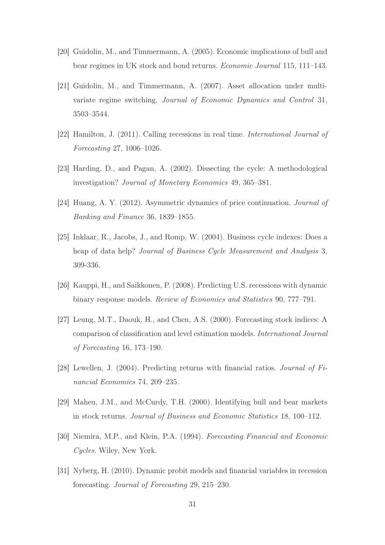
Table 8 reports the portfolio returns from the best probit models selected in

terms of their in-sample and out-of-sample predictive performances presented in

Sections 4.2 and 4.3. We also consider the benchmark model of Chen (2009) in-

cluding the term spread and inflation as predictors. The results show that the

annualized average returns in the best probit models are clearly higher than in

the B&H strategy (6.04%). As an example, the best model in terms of the out-of-

10 More complicated trading strategies, which possibly employ also forecasts for the longer

forecast horizons using, for example, the procedures proposed by Guidolin and Timmermann

(2005, 2007) and Guidolin and Hyde (2012), are left for the future research. Furthermore, in the

market timing experiment the risk-free interest rate is approximated by using the three-month

Treasury Bill rate (it).

26

sample forecasts (the autoregressive model (4) with the predictors given in (10))

yields the annualized returns 6.77% and 7.00% when the thresholds ζ = 0.50 and

ζ = y are employed, respectively. The return from the third strategy, where the

portfolio weight is the probability of the bear market, is 6.88%.

In line with the statistical forecast evaluation measures, the results confirm

that the highest portfolio returns are typically obtained with the dynamic models

which are predicting the state of the stock market more accurately than the static

model (3) (cf. the percentages of correct forecasts (CR50% and CRy%) reported in

Table 8). In the dynamic models, more profitable trading strategies are obtained

when the sample average (ζ = y) is used as a threshold. This is presumably related

to the fact that the bear market probability is typically lower than 50% most of the

time. Thus, the 50% threshold will likely lead to the excessive number of missing

bear market signals. As a whole, the dynamic autoregressive model (5) seems to

produce somewhat higher portfolio returns than the autoregressive model (4). It

is also worth noting that the static model (3) turns out to perform relatively well

when the 50% threshold (ζ=0.50) is employed. However, the results with other two

weighting schemes clearly show the superior portfolio performance of the dynamic

models over the static model.

As different trading strategies involve different levels of risk, it is also of interest

to consider risk-adjusted returns. The numbers in the parentheses in Table 8 are

the Sharpe ratios measuring the risk-adjusted returns.11 Portfolios and trading

strategies with a high Sharpe ratio (higher return over the volatility of returns)

are preferable to those with a low Sharpe ratio. Overall, the reported Sharpe ratios

are in line with the annualized percentage returns. In particular, the Sharpe ratios

in the best dynamic models are substantially higher than in the B&H strategy. In

fact, the differences appear to be even larger than in the unadjusted returns.

Overall, the main message from this simple trading strategy is that the prob-

ability forecasts for the bear and bull markets are also useful in the portfolio

management point of view. An investor can clearly do better by holding her assets

11 The Sharpe ratio (SR) is defined as SR = (Rk −Rrf)/σk, where Rk is the annualized return

from model k, Rrf is the risk-free return and σk is the standard deviation of portfolio returns

based on the model k.

27

at the risk-free interest rate when the probability of the bear market is relatively

high and invest in stocks when the probability is low.

5 Conclusions

This study compares the forecast performance of the standard static and more

advanced dynamic binary time series models to predict the U.S. bear and bull

stock markets. To facilitate these comparisons, we first extract the turning points,

peaks and troughs, of the U.S. stock market using the information which was

available to investors in real time in the past. The obtained turning points are

compared with the reference dates proposed in the previous studies and found

similar to them. In forecasting part of the paper, we examine a comprehensive

monthly data set of macroeconomic and financial variables to predict the future

state of the U.S. stock market when using the static and dynamic probit models.

Results show that the U.S. bear and bull markets are predictable in and out

of sample. Dynamic probit models tend to yield superior forecasts compared with

the static model. This improvement in out-of-sample forecast accuracy is not sur-

prising given that the dynamic models were found to take the dynamics of the

regime switches between the bear and bull markets into account in an adequate

way. In addition to the statistical goodness-of-fit measures, the portfolio returns

based on the forecasts of the best dynamic probit models are also higher than

the returns obtained with the passive buy-and-hold strategy in the simple trading

simulation experiment. As far as the predictive variables are concerned, the past

stock returns, the term spread between the long-term and short-term interest rates

and the dividend-price ratio appear to be the best leading indicators for the future

state of the stock market. The best out-of-sample forecasts are obtained when all

of these predictors are employed together in the dynamic models.

The evidence of predictability of the bear and bull markets, as shown in this

study, have many interesting further implications and potential extensions in em-

pirical finance research. For example, linking the bear and bull market predictabil-

ity to the momentum profits and their dynamics between different states of the

stock market could be an interesting extension (cf. the findings of Cooper et al.

28

(2004), Asem and Tian (2010) and Huang (2012)). Furthermore, the predictability

of the market status may also provide new insights into the empirical implemen-

tation of the asset pricing models accommodating regime switches (see, e.g., the

survey of Ang and Timmermann, 2011) as well as strategic asset allocation deci-

sions under the presence of regimes in stock returns (cf. Guidolin and Timmermann

(2007), Tu (2010) and Guidolin and Hyde (2012)).

References

[1] Anatolyev, S., and Gospodinov, N. (2010). Modeling financial return dynamics

via decomposition. Journal of Business and Economic Statistics 28, 232–245.

[2] Ang, A., and Bekaert, G. (2007). Stock return predictability: Is it there?

Review of Financial Studies 20, 651–707.

[3] Ang, A., and Timmermann, A. (2011). Regime changes and financial markets.

NBER Working Paper, No. 17182.

[4] Asem, E., and Tian, G.Y. (2010). Market dynamics and momentum profits.

Journal of Financial and Quantitative Analysis 45, 1549–1562.

[5] Berge, T., and Jorda, O. (2011). Evaluating the classification of economic ac-

tivity into recessions and expansions. American Economic Journal: Macroe-

conomics 3, 246–277.

[6] Bry G., and Boschan, C. (1971). Cyclical analysis of time series: Selected

procedures and computer programs. National Bureau of Economic Research,

Columbia University Press.

[7] Campbell, J.Y., and Shiller, R.J. (1988). Stock prices, earnings, and expected

dividends. Journal of Finance 43, 661–676.

[8] Campbell, J.Y., and Thompson, S.B. (2008). Predicting excess stock returns

out of sample: Can anything beat the historical average? Review of Financial

Studies 21, 1509–1532.

29

[9] Candelon B, Piplack, J., and Straetmans, S. (2008). On measuring synchro-

nization of bulls and bears: The case of East Asia. Journal of Banking and

Finance 32, 1022–1035.

[10] Chauvet, M., and Piger, J. (2008). A comparison of the real-time performance

of business cycle dating methods. Journal of Business and Economic Statistics

26, 42–49.

[11] Chauvet, M., and Potter, S. (2000). Coincident and leading indicators of the

stock market. Journal of Empirical Finance 7, 87–111.

[12] Chauvet, M., and Potter, S. (2005). Forecasting recession using the yield

curve. Journal of Forecasting 24, 77–103.

[13] Chen, S.S. (2009). Predicting the bear market: Macroeconomic variables as

leading indicators. Journal of Banking and Finance 33, 211–223.

[14] Cooper, M.J., Gutierrez Jr., R.G., and Hameed, A. (2004). Market states and

momentum. Journal of Finance 59, 1345–1365.

[15] Diebold, F.X., and Mariano, R.S. (1995). Comparing predictive accuracy.

Journal of Business and Economic Statistics 13, 253–263.

[16] Diebold, F.X., and Rudebusch, G.D. (1989). Scoring the leading indicators.

Journal of Business 62, 369–391.

[17] Estrella, A. (1998). A new measure of fit for equations with dichotomous

dependent variables. Journal of Business and Economic Statistics 16, 198–

205.

[18] Estrella A., and Mishkin, F.S. (1998). Predicting U.S. recessions: Financial

variables as leading indicators. Review of Economics and Statistics 80, 45–61.

[19] Guidolin, M., and Hyde, S. (2012). Can VAR models capture regime shifts in

asset returns? A long-horizon strategic asset allocation perspective. Journal

of Banking and Finance 36, 695–716.

30

[20] Guidolin, M., and Timmermann, A. (2005). Economic implications of bull and

bear regimes in UK stock and bond returns. Economic Journal 115, 111–143.

[21] Guidolin, M., and Timmermann, A. (2007). Asset allocation under multi-

variate regime switching. Journal of Economic Dynamics and Control 31,

3503–3544.

[22] Hamilton, J. (2011). Calling recessions in real time. International Journal of

Forecasting 27, 1006–1026.

[23] Harding, D., and Pagan, A. (2002). Dissecting the cycle: A methodological

investigation? Journal of Monetary Economics 49, 365–381.

[24] Huang, A. Y. (2012). Asymmetric dynamics of price continuation. Journal of

Banking and Finance 36, 1839–1855.

[25] Inklaar, R., Jacobs, J., and Romp, W. (2004). Business cycle indexes: Does a

heap of data help? Journal of Business Cycle Measurement and Analysis 3,

309-336.

[26] Kauppi, H., and Saikkonen, P. (2008). Predicting U.S. recessions with dynamic

binary response models. Review of Economics and Statistics 90, 777–791.

[27] Leung, M.T., Daouk, H., and Chen, A.S. (2000). Forecasting stock indices: A

comparison of classification and level estimation models. International Journal

of Forecasting 16, 173–190.

[28] Lewellen, J. (2004). Predicting returns with financial ratios. Journal of Fi-

nancial Economics 74, 209–235.

[29] Maheu, J.M., and McCurdy, T.H. (2000). Identifying bull and bear markets

in stock returns. Journal of Business and Economic Statistics 18, 100–112.

[30] Niemira, M.P., and Klein, P.A. (1994). Forecasting Financial and Economic

Cycles. Wiley, New York.

[31] Nyberg, H. (2010). Dynamic probit models and financial variables in recession

forecasting. Journal of Forecasting 29, 215–230.

31

[32] Nyberg, H. (2011). Forecasting the direction of the U.S. stock market with

dynamic binary probit models. International Journal of Forecasting 27, 561–

578.

[33] Pagan, A.R., and Sossounov, K.A. (2003). A simple framework for analyzing

bull and bear markets. Journal of Applied Econometrics 18, 23–46.

[34] Rapach, D.E., Wohar, M.E., and Rangvid, J. (2005). Macro variables and

international stock return predictability. International Journal of Forecasting

21, 137–166.

[35] Rydberg, T., and Shephard, N. (2003). Dynamics of trade-by-trade price

movements: Decomposition and models. Journal of Financial Econometrics

1, 2–25.

[36] Tu, J. (2010). Is regime switching in stock returns important in portfolio

decisions? Management Science 56, 1198–1215.

32

Figures and Tables

Table 1: Turning points of the U.S. stock market.

Peaks Troughs Bull Bull Bull Bear Bear Bear

duration Change% Publication duration Change% Publication

(months) lag (months) lag

(1957:12)

1959:7 1960:10 19 51.31 8 15 -11.77 5

1961:12 1962:6 14 34.01 4 6 -23.48 10

1966:1 1966:9 43 69.64 5 8 -17.57 6

1968:11 1970:6 26 41.55 7 19 -32.30 6

1972:12 1974:9 30 62.34 4 21 -46.18 8

1976:12 1978:2 27 69.12 2 14 -19.00 6

1980:11 1982:7 33 61.44 9 20 -23.79 4

1983:6 1984:5 11 56.54 9 11 -10.19 6

1987:8 1987:11 39 119.06 – 3 -30.17 –

1990:5 1990:10 30 56.85 3 6 -15.84 6

2000:8 2003:2 118 399.24 3 30 -44.58 5

2007:10 2009:2 56 84.20 3 16 -52.56 8

Notes: The first (second) column gives the peak (trough) turning points of the S&P500 index

determined by the Bry-Boschan (1971) dating method. Additionally, an extra peak and trough

month has been assigned to the year 1987. The sample period is 1957:1–2010:12. A bear market

starts after the peak month and ends at the trough, and vice versa with a bull market. Bull

(bear) duration shows the time in months from the last trough (peak) to the next peak

(trough). The percentage change in the S&P500 index during the bear and bull market is

denoted by “Change%”. The publication lag is the time between the turning point month (peak

or trough) and the month when it has been identified by the Bry-Boschan algorithm employed

sequentially using only the information which was available in real time.

33

Table 2: Monthly U.S. data set.

Variable Description

rt One-month return in the S&P500 index (log-difference)

FFt Federal Funds rate

it Three-month U.S. Treasury Bill rate, secondary market

R5yt 5-year U.S. Treasury Bond rate, constant maturity

R10yt 10-year U.S. Treasury Bond rate, constant maturity

∆FFt, ∆it, ∆R10yt First differences of FFt, it and R10y

t

TSt Term spread, TSt = R10yt − it

Y St Yield spread, Y St = R5yt − it

∆URt The first difference of the U.S. civilian unemployment rate

∆IPt 12-month log-difference of the U.S. industrial production

INFt U.S.Inflation rate, 12-month log-difference of the CPI

DPt Dividends over the past year divided by the current S&P500 index

EPt Earnings over the past year divided by the S&P500 index

∆DPt, ∆EPt First differences of DPt and EPt

Notes: The sample period is from January 1957 to December 2010. Monthly S&P500 index,

interest rates, unemployment, inflation and industrial production are obtained from the Federal

Reserve Bank of St. Louis databank (FRED). Dividends Dt and earnings Et are obtained from

the homepage of Robert Shiller’s book Irrational exuberance (see

http://www.irrationalexuberance.com) [Accessed November 2011].

34

Table 3: In-sample pseudo-R2 values of the static model (3) and the autoregressive

model (4).

xt−h h = 1 h = 2 h = 3 h = 4 h = 5 h = 6 h = 12

rt−h static 0.101 0.054 0.031 0.028 0.025 0.012 0.000

auto 0.229 0.136 0.089 0.066 0.045 0.024 0.001

TSt−h static 0.028 0.034 0.037 0.039 0.039 0.039 0.052

auto 0.150 0.151 0.151 0.150 0.150 0.149 0.134

Y St−h static 0.023 0.029 0.033 0.034 0.034 0.034 0.044

auto 0.149 0.148 0.147 0.146 0.144 0.142 0.124

∆it−h static 0.000 0.000 0.000 0.002 0.005 0.002 0.000

auto 0.005 0.006 0.007 0.008 0.007 0.003 0.002

∆FFt−h static 0.001 0.003 0.003 0.005 0.006 0.002 0.003

auto 0.082 0.082 0.079 0.075 0.007 0.004 0.055

∆R10yt−h static 0.007 0.003 0.002 0.005 0.012 0.011 0.000

auto 0.079 0.074 0.071 0.070 0.027 0.017 0.001

INFt−h static 0.027 0.024 0.022 0.020 0.017 0.015 0.009

auto 0.028 0.026 0.023 0.021 0.018 0.017 0.010

∆IPt−h static 0.001 0.003 0.007 0.010 0.013 0.017 0.004

auto 0.008 0.010 0.013 0.014 0.016 0.017 0.001

∆URt−h static 0.006 0.003 0.000 0.000 0.002 0.002 0.001

auto 0.008 0.003 0.002 0.004 0.005 0.004 0.001

∆DPt−h static 0.092 0.047 0.026 0.023 0.017 0.009 0.002

auto 0.184 0.104 0.064 0.045 0.028 0.014 0.057

∆EPt−h static 0.027 0.010 0.004 0.004 0.003 0.001 0.006

auto 0.035 0.016 0.002 0.001 0.002 0.015 0.043

Notes: Table reports the values of the pseudo-R2 measure (see (9)) in different probit models.

The models include one predictive variable given in the first column of the table. The predictive

variables are introduced more detail in Table 2. In the table, “static” denotes the static probit

model (3) and “auto” is the autoregressive model (4). The underlying forecast horizon h is given

in the first row.

35

Table 4: In-sample pseudo-R2 values of the dynamic autoregressive model (5).

xt−h h = 1 h = 2 h = 3 h = 4 h = 5 h = 6 h = 12

rt−h 0.793 0.791 0.788 0.783 0.783 0.787 0.783

TSt−h 0.791 0.787 0.787 0.785 0.784 0.784 0.785

Y St−h 0.790 0.787 0.786 0.784 0.784 0.784 0.784

∆it−h 0.790 0.783 0.783 0.787 0.789 0.784 0.783

∆FFt−h 0.788 0.787 0.783 0.785 0.784 0.784 0.783

∆R10yt−h 0.786 0.784 0.783 0.786 0.792 0.783 0.785

INFt−h 0.783 0.783 0.783 0.783 0.783 0.783 0.783

∆IPt−h 0.788 0.787 0.787 0.785 0.785 0.785 0.784

∆URt−h 0.783 0.784 0.785 0.789 0.785 0.783 0.783

∆DPt−h 0.796 0.791 0.788 0.783 0.783 0.785 0.783

∆EPt−h 0.794 0.789 0.786 0.783 0.783 0.785 0.784

Notes: Table reports the values of the pseudo-R2 measure (see (9)) of the dynamic

autoregressive model (5) including one predictive variable given in the first column of the table.

See also notes to Table 3.

36

Table 5: Estimation results of the best in-sample predictive models.

static static auto. dyn.auto.

model (3) model (3) model (4) model (5)

constant -0.656 -0.639 0.012 -1.828

(0.257) (0.256) (0.016) (0.262)

πt−1 0.959 -0.026

(0.007) (0.081)

yt−1 4.089

(0.294)

rt−1 -0.909 -5.438 6.983

(0.011) (1.064) (2.061)

TSt−1 -0.136 -0.132 -0.044 -0.226

(0.093) (0.093) (0.010) (0.098)

∆DPt−8 0.251 -2.448 -1.671

(0.381) (0.391) (0.742)

INFt−1 0.057 0.051 0.008 -0.027

(0.042) (0.042) (0.002) (0.038)

log-L -350.742 -320.989 -230.575 -88.661

pseudo-R2 0.041 0.135 0.412 0.807

QPS 0.376 0.369 0.240 0.071

BIC 360.397 337.079 249.883 111.188

CR50% 0.731 0.729 0.821 0.960

CRy% 0.641 0.663 0.798 0.962

Notes: The models are estimated using the data from 1957:1 to 2010:12. Robust standard errors

given in parentheses are computed with the procedures suggested by Kauppi and Saikkonen

(2008). In addition to the QPS and pseudo-R2 statistics (see (8) and (9)), Schwarz information

criterion (BIC) is also reported. In the table, CR50% and CRy% are the percentages of correct

forecasts when the thresholds ζ = 0.5 and ζ = y are used to construct signal forecasts (see

Section 3.3).

37

Table 6: Out-of-sample QPS statistics in the best probit models with one predictor.

xt−h h = 1 h = 2 h = 3 h = 4 h = 5 h = 6 h = 12

rt−h static 0.302 0.313 0.325 0.327 0.328 0.336 0.351

auto 0.229 0.266 0.294 0.308 0.321 0.334 0.446

d.auto 0.276 0.295 0.298 0.295 0.305 0.327 0.357

TSt−h static 0.347 0.342 0.336 0.330 0.326 0.322 0.307

auto 0.297 0.293 0.290 0.288 0.298 0.293 0.308

d.auto 0.235 0.247 0.258 0.278 0.293 0.314 0.358

Y St−h static 0.311 0.314 0.319 0.322 0.324 0.329 0.312

auto 0.299 0.298 0.300 0.297 0.296 0.296 0.313

d.auto 0.234 0.254 0.261 0.282 0.288 0.309 0.351

∆it−h static 0.348 0.348 0.349 0.350 0.352 0.348 0.347

auto 0.358 0.351 0.371 0.379 0.371 0.341 0.349

d.auto 0.255 0.264 0.284 0.301 0.319 0.315 0.355

∆FFt−h static 0.350 0.352 0.352 0.351 0.350 0.347 0.352

auto 0.354 0.348 0.343 0.347 0.337 0.328 0.349

d.auto 0.253 0.271 0.282 0.298 0.310 0.317 0.352

∆R10yt−h static 0.353 0.351 0.348 0.349 0.351 0.349 0.345

auto 0.343 0.336 0.352 0.361 0.360 0.352 0.343

d.auto 0.250 0.264 0.280 0.292 0.305 0.318 0.360

INFt−h static 0.326 0.327 0.328 0.329 0.330 0.332 0.338

auto 0.326 0.327 0.328 0.329 0.331 0.331 0.338

d.auto 0.247 0.265 0.281 0.295 0.308 0.318 0.346

∆IPt−h static 0.373 0.377 0.378 0.378 0.377 0.374 0.351

auto 0.382 0.381 0.380 0.378 0.376 0.374 0.352

d.auto 0.269 0.286 0.298 0.309 0.316 0.326 0.392

∆URt−h static 0.340 0.344 0.347 0.352 0.354 0.353 0.348

auto 0.339 0.379 0.383 0.388 0.392 0.396 0.349

d.auto 0.247 0.264 0.279 0.300 0.309 0.319 0.353

∆DPt−h static 0.309 0.322 0.331 0.333 0.335 0.339 0.348

auto 0.367 0.363 0.359 0.357 0.353 0.351 0.376

d.auto 0.241 0.265 0.278 0.296 0.306 0.320 0.353

∆EPt−h static 0.361 0.356 0.353 0.350 0.347 0.346 0.343

auto 0.371 0.372 0.375 0.376 0.375 0.372 0.369

d.auto 0.245 0.264 0.283 0.296 0.314 0.317 0.356

Notes: Table reports the out-of-sample QPS statistics (see (8)) in different probit models. In

the table, “static” denotes the static probit model (3), “auto” is the autoregressive model (4)

and “d.auto” is the dynamic autoregressive model (5).

38

Table 7: Out-of-sample QPS statistics in the selected models.

xt−h model h = 1 h = 2 h = 3 h = 4 h = 5 h = 6 h = 12

(TSt−h, INFt−h) static 0.336 0.334 0.331 0.326 0.322 0.319 0.307

auto 0.306 0.332 0.328 0.324 0.295 0.293 0.307

d.auto 0.241 0.250 0.261 0.278 0.294 0.314 0.359

(rt−h, TSt−h) static 0.300 0.310 0.320 0.315 0.312 0.315 0.314

auto 0.223 0.259 0.283 0.293 0.301 0.305 0.437

d.auto 0.267 0.281 0.280 0.278 0.293 0.318 0.354

(rt−h, TSt−h, ∆DPt−8) static 0.299 0.311 0.321 0.316 0.313 0.316 0.299

auto 0.184 0.228 0.250 0.262 0.274 0.288 0.411

d.auto 0.264 0.279 0.270 0.269 0.282 0.312 0.346

(rt−h, TSt−h, ∆DPt−8, INFt−h) static 0.293 0.305 0.317 0.313 0.311 0.314 0.295

auto 0.243 0.269 0.276 0.280 0.283 0.286 0.292

d.auto 0.273 0.291 0.276 0.270 0.283 0.312 0.348

Notes: Table reports the out-of-sample QPS measures in the selected probit models with two or

more predictors. The best models obtained in the model selection (see Section 4.2) including

the predictors (10) and (11) are presented at the bottom of the table. See also notes to Table 6.

39

Table 8: Portfolio returns from different probit models and trading strategies.

ζ = 0.50 ζ = y pt+h

xt−h model annual return CR50% annual return CRy% annual return

(Sharpe ratio) (Sharpe ratio) (Sharpe ratio)

B&H 6.04 (0.48) 6.04 (0.48) 6.04 (0.48)

strategy

rt−1 static 7.68 (0.91) 0.833 4.14 (0.18) 0.659 6.04 (0.72)

auto 8.25 (1.09) 0.873 5.63 (0.61) 0.774 6.39 (0.63)

d.auto 7.85 (0.97) 0.841 7.71 (1.02) 0.849 6.60 (0.83)

TSt−1 static 6.07 (0.48) 0.797 5.23 (0.39) 0.571 5.63 (0.54)

auto 6.07 (0.48) 0.798 6.21 (0.61) 0.698 6.03 (0.63)

d.auto 7.36 (0.80) 0.829 8.07 (1.14) 0.857 6.62 (0.82)

(rt−1, TSt−1) static 7.73 (0.89) 0.825 5.06 (0.40) 0.675 6.10 (0.70)

auto 7.79 (0.98) 0.873 6.61 (0.84) 0.813 6.58 (0.88)

d.auto 6.92 (0.68) 0.813 7.94 (0.97) 0.829 6.70 (0.77)

(INFt−1, TSt−1) static 6.07 (0.48) 0.798 6.38 (0.63) 0.631 5.79 (0.57)

auto 6.08 (0.48) 0.798 7.17 (0.81) 0.736 6.05 (0.63)

d.auto 5.40 (0.35) 0.806 8.76 (1.30) 0.829 6.59 (0.78)

(rt−1, TSt−1, static 7.62 (0.86) 0.829 5.06 (0.40) 0.674 6.14 (0.71)

∆DPt−8) auto 6.77 (0.68) 0.877 7.00 (0.92) 0.873 6.88 (0.92)

d.auto 6.27 (0.55) 0.817 7.41 (0.88) 0.810 6.70 (0.81)

(rt−1, TSt−1, static 7.55 (0.85) 0.837 5.45 (0.50) 0.698 6.24 (0.73)

∆DPt−8, INFt−1) auto 6.74 (0.64) 0.821 7.82 (0.90) 0.861 6.88 (0.76)

d.auto 6.24 (0.55) 0.821 7.44 (0.94) 0.778 6.57 (0.79)

Notes: The returns presented in the table are the average annualized portfolio returns from the

buy-and-hold (B&H) strategy and from a simple trading strategy between stock and risk-free

interest rate investments where the asset allocation decision is based on the forecasts obtained

with different probit models. The thresholds used to obtain investment signals are the 50% rule

(ζ = 0.50) and the sample mean of yt (ζ = y). In the third strategy, the asset allocation is

directly based on the probability forecast of the bear market (denoted by pt+h). The values of

the (annualized) Sharpe ratios are given in parentheses. Furthermore, CR50% and CRy% are the

percentages of correct forecasts when the thresholds ζ = 0.5 and ζ = y are used, respectively.

See also notes to Table 6.

40

55 60 65 70 75 80 85 90 95 00 05 10 15Time

Log(

S&

P50

0)

3.5

4

4.5

5

5.5

6

6.5

7

7.5

Figure 1: The U.S. bear (shaded areas) and bull stock markets with the log of the

S&P500 index.

41

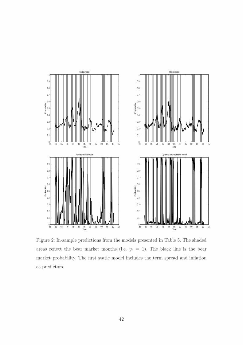
55 60 65 70 75 80 85 90 95 00 05 10 15Time

Static model

Pro

babili

ty

0

0.1

0.2

0.3

0.4

0.5

0.6

0.7

0.8

0.9

1

55 60 65 70 75 80 85 90 95 00 05 10 15Time

Pro

babili

ty

Static model

0

0.1

0.2

0.3

0.4

0.5

0.6

0.7

0.8

0.9

1

55 60 65 70 75 80 85 90 95 00 05 10 15Time

Pro

babili

ty

Autoregressive model

0

0.1

0.2

0.3

0.4

0.5

0.6

0.7

0.8

0.9

1

55 60 65 70 75 80 85 90 95 00 05 10 15Time

Pro

babili

ty

Dynamic autoregressive model

0

0.1

0.2

0.3

0.4

0.5

0.6

0.7

0.8

0.9

1

Figure 2: In-sample predictions from the models presented in Table 5. The shaded

areas reflect the bear market months (i.e. yt = 1). The black line is the bear

market probability. The first static model includes the term spread and inflation

as predictors.

42

88 90 92 94 96 98 00 02 04 06 08 10 120

0.1

0.2

0.3

0.4

0.5

0.6

0.7

0.8

0.9

1

Time

Pro

ba

bility

Static model

88 90 92 94 96 98 00 02 04 06 08 10 120

0.1

0.2

0.3

0.4

0.5

0.6

0.7

0.8

0.9

1

TimeP

robabili

ty

Static model

88 90 92 94 96 98 00 02 04 06 08 10 120

0.1

0.2

0.3

0.4

0.5

0.6

0.7

0.8

0.9

1

Time

Pro

babili

ty

88 90 92 94 96 98 00 02 04 06 08 10 120

0.1

0.2

0.3

0.4

0.5

0.6

0.7

0.8

0.9

1

Time

Pro

babili

ty

Autoregressive model

88 90 92 94 96 98 00 02 04 06 08 10 120

0.1

0.2

0.3

0.4

0.5

0.6

0.7

0.8

0.9

1

Time

Pro

babili

ty

Dynamic autoregressive model

Figure 3: Out-of-sample forecasts from the probit models with the predictors given

in (10) except the first static model which includes the term spread and inflation.

The shaded areas depict the bear stock market periods. The black line is the bear

market probability. The forecast horizon is one month (h = 1) and the dashed line

is the time-varying mean threshold (i.e. ζ = y) showing the sample average of the

bear market months.

43