Predictability Puzzles - Marginal Qeraker.marginalq.com/predPuzzles.pdf · Predictability Puzzles Bj˝rn Eraker March 19, 2017 ... is, the equilibrium log price-dividend ratio is

Predictability Puzzles

Bjørn Eraker ∗

March 19, 2017

Abstract

Dynamic equilibrium models based on present value computation imply that returns are

predictable, suggesting that time-series that predict returns could be priced risk factors.

Equilibrium models however, imply that returns from risk-based state-variables are pre-

dictable in the short, but not the long-run. The variables that have been shown empirically

to predict returns typically do so at medium or long horizons, and never at short horizons.

This contradicts the equilibrium interpretation. I develop econometric tests aimed at test-

ing whether predictive variables show term structures of predictability that is consistent

with equilibrium. Empirically, I find that the variables in question are either not significant

predictors, or the predictability fails to be consistent with equilibrium.

Preliminary draft.

Comments welcomed.

∗Wisconsin School of Business, Department of Finance. Bjørn Eraker ([email protected]). I thank IvanShaliastovich, Sang Byung Seo and seminar participants at the University of Wisconsin and the Midwest FinanceAssociation 2017 Annual Meeting for helpful comments. All errors are my own.

1

1 Introduction

Very few topics in Finance is as heavily researched and hotly contested as predictability of

asset returns. Fama and French (1988) and Campbell and Shiller (1988b) were among the

first to document predictability of stock returns from price-dividend ratios. Fama and French

(1988a) find that the price-dividend ratio predicts an increasing term structure of regression

R2s. There is no predictability at the short horizon (month or quarter) and the R2s increase

monotonically to somewhere between 13% and 49% at the five year forecasting horizon. The

long range predictability of returns from price-dividend ratios has been considered so compelling

that Cochrane (1999), in his essay entitled “New Facts in Finance”, declared it a fact.

Not only does predictability of returns from price-dividend ratios seem statistically and eco-

nomically significant, it is also logically consistent with equilibrium under time-varying expected

returns. Indeed, Fama and French (1988) recognize this and write that “The hypothesis that

D/P forecasts returns has a long tradition among practitioners and academics ... The intuition of

the ’efficient markets’ version of the hypothesis is that stock prices are low relative to dividends

when discount rates and expected returns are high, and vice versa, so that D/P varies with

expected returns.” This intuition is precisely the main mechanism that leads to time-variation

in expected returns in modern dynamic models of asset prices. Campbell and Shiller (1988b),

Campbell and Shiller (1988a) specify econometric models of dividend discounting that imply

that price dividend ratios predict stock returns. This is also a fundamental property of dynamic

equilibrium models such as Bansal and Yaron (2004), Campbell and Cochrane (1999), Menzly,

Santos, and Veronesi (2004) and numerous others. In this literature, typically, (log) dividends

and (log) prices contain unit roots but are co-integrated with co-integration vector [0, 1]. That

is, the equilibrium log price-dividend ratio is a linear function of stationary state-variables Xt,

as the equilibrium takes on the form

lnPt/Dt = α + β′Xt. (1)

The unit root behavior of (log) prices and dividends and the stationarity of Xt implies that the

right hand side of (1) predicts returns. Intuitively, when P/D ratios are high, the expected rate

of return going forward is low and vice versa, as suggested in the above quote to Fama and

French (1998a).

In this paper I take issue with the idea that the evidence presented in favor of return pre-

dictability is consistent with equilibrium. Rather, I argue that equilibrium models

2

1. generate more predictability at short forecasting horizons than long, which is precisely the

opposite of what we find in the data, and

2. imply that positive (negative) shocks to expected return contemporaneously correlate neg-

atively (positively) with prices. Yet, variables that have been shown to predict returns

have insignificant contemporaneous return correlation. Conversely, implied volatility has

significant negative correlation with returns but does not predict returns.

The intuition regarding the first point goes as follows: Imagine an economy where a time-varying

risk factor (let’s say volatility) generates time-variation in expected return. If risk is high today,

the equilibrium expected rate of return must be high today as well. For equilibrium to prevail in

high volatility states it must be that investors are compensated for the above-average risk. Yet,

we find no evidence of such short term risk premium in the data.

Moreover, long horizon predictability is not consistent with intertemporal equilibrium. To

see this, consider an investor who observes high risk today but expect to be rewarded four or

five months down the road. It’s clearly optimal for such an investor to wait to four months

to invest, thereby avoiding low reward-to-risk regime today and exploiting a high reward-to-

risk regime in the future. Clearly this cannot be an equilibrium. Another way to think about

the counterintuitive nature of long-but-not-short-term predictability is to consider the investor’s

investment rule. He or she simply has to discard recent information and look back, say, four or

five months at the market conditions at that time to make current investment decisions. This

essentially implies that the the relevant state-variable(s) that govern the investors’ investment

decisions do not follow Markov processes. This is inconsistent with standard equilibrium models

and it is hard to imagine what kind of economic environment that would support this kind of

delayed price response in an rational equilibrium model.

The second bullet point above is related to the fact that equilibrium prices respond negatively

(positively) to positive (negative) shocks in expected returns. In the time-varying volatility lit-

erature this is referred to as a “volatility feedback effect.” Many of the variables that have been

shown to predict returns have economically and statistically insignificant contemporaneous corre-

lation with returns. For example, Bollerslev, Tauchen, and Zhou (2009) show that the difference

between physical and option implied volatility, known as the variance risk premium (VRP) in the

literature, significantly predicts returns at horizons four-five month horizons. But the VRP does

not predict returns at short forecasting horizons. It also has fairly low contemporaneous corre-

lation with returns. This, along with the lack of short term predictability and strong medium

to long term predictability each point to the VRP as showing predictability patterns that are

inconsistent with equilibrium.

3

To make these arguments precise I quantify the relationship between the predictable variation

in returns and the contemporaneous correlation between changes in the predictor and the returns.

I derive simple algebraic relations that imposes the equilibrium structure onto the predictive

regression coefficients. I then derive t tests for the difference between the estimated predictive

coefficients and the equilibrium implied coefficients.

I apply my empirical tests to a range of time-series variables that have been shown to predict

stock returns in the extant literature. Using monthly time-series going back to the 1920ties, I

show that the level of interest rates (3m TBILL rate), slope of the yield curve and default spread

are either insignificant predictors at all, or if they are significantly predicting stock returns, the

term structure of predictability tend to be inconsistent with equilibrium. The strongest predictors

are term structure slope (at the monthly frequency) and VRP at the daily frequency. Nether of

these variables predict stock returns at short horizons. The lack of short term predictability is

inconsistent with equilibrium where a time-varying risk premium is proportional to some mean-

reverting risk variable. Rather, most of the predictable variation I find is for horizons that exceed

3-5 months. Virtually all the predictors show a monotonically increasing predictability pattern, at

least for some sub-group of forecasting horizons. These patterns are consistent with predictability

generated by sampling variation as suggested by Boudoukh, Richardson, and Whitelaw (2006)

rather than dynamic equilibrium.

Shocks to VIX or VIX squared are very highly negatively correlated with returns. This in

itself suggests VIX squared is a good candidate for a priced risk variable. Again however, the

empirical tests are not kind to this interpretation: using first a test based on the idea that shocks

to the state variable (squared VIX in this case) should be negatively correlated with returns in

equilibrium, I show that the null of equilibrium consistency is sharply rejected. In short, the VIX

ought to predict returns at short horizons, but it does not. The result is that investors are forced

to hold assets in volatile times without compensation for this additional risk - an implication

that cannot be reconciled with equilibrium. The same conclusion holds whether or not I use

measures of physical or option implied variance. The findings echo Moreira and Muir (2017)’s

finding that selling stock in volatile times and buying in low volatility times improves the Sharpe

ratio of investors.

The remainder of the paper is organized as follows. In the next section I postulate a very

simple equilibrium relation between dividends, prices and a state-variables that generate fluc-

tuations in expected returns. I show that without imposing a specific equilibrium structure I

can derive equilibrium-implied predictive coefficients that can be compared to estimated, reduced

form predictive coefficients. I discuss empirical tests to compare the two. In section three I apply

4

the tests to monthy and daily sampled data on candidate predictors/ risk-variables. Section 4

discusses the findings concludes.

2 A test for dynamic consistency

In the following I derive tests of whether the predictable pattern from a time-series, say xt, to i

period ahead returns rt+i is consistent with dynamic equilibrium. Standard dynamic equilibrium

models dictate that the price obtains as a present value of future dividends. This again implies

that the price-dividend ratio is a function of the state-variable xt,

PtDt

= F (xt). (2)

This equation just implies that the price is degree one homogenous in dividends. Consistent with

Long-Run-Risk, habit formation, and other equilibrium models we assume that F is exponential

affine

F (x) = eα+βxt (3)

such that the log-price dividend ratio is

lnPt = lnDt + α + βxt. (4)

Since dividends contain a unit root, this equation implies that log prices and log dividends are

cointegrated. The cointegrating relationship between dividends and prices is not important per

se in our context. However, eqn. (4) suggests that prices contain a temporary component driven

by the risk variable xt. This variable predicts stock returns. It does so by temporarily moving the

price away from its steady state path. To see how shocks to xt generates time-varying expected

rates of return, assume that log-dividend growth rates are given by

lnDt+1 − lnDt = µ+ ωxt + εt+1 (5)

where a non-zero ω implies that the state-variable drives expected dividends, as in Bansal-Yaron

(2004).

The dynamics of log capital gains follow

lnPt+1 − lnPt = µ+ ωxt + β(xt+1 − xt) + εt+1. (6)

5

This equation suggests that estimates of ω and β can be obtained through a regression of log

capital gains onto xt and 4xt+1 = xt+1 − xt. Alternatively, estimates of ω can be obtained by

regressing log-dividend growth on x.

The h period ahead capital gain is given by

lnPt+h − lnPt = µh+ ω

h∑i=1

xt+i + β(xt+h − xt) +h∑i=1

εt+i (7)

The expected h period capital gain can be found by taking expectations of (7). In the case that

x follows an AR(1) with autocorrelation ρ it is

Et [lnPt+h − lnPt] = µh+

[ωρh+1 − ρρ− 1

+ β(ρh − 1)

]xt. (8)

Equation (8) suggests that if one were to run the regression

lnPt+h − lnPt = ah + bhxt + uht (9)

the intercept and slope would have to satisfy

ah = µh, (10)

bh =

[ωρh+1 − ρρ− 1

+ β(ρh − 1)

]. (11)

Notice that these equations impose testable restrictions. In particular, the entire term structure of

predictable variation in returns is governed by the feedback coefficient β and the autocorrelation,

ρ, of the predictor variable. I will argue below, ω is practically very small and I ignore it in the

empirical implementation of my tests. This leaves a very simple structural restriction on the

predictive coefficients

bh = β(ρh − 1) (12)

This is valid under an AR(1) assumption for the state-variable. More generally, under an AR(p)

assumption we have Etxt+h = Chxt where Ch = Corr(xt+h, xt) in which case the restriction

becomes

bh = β(Ch − 1). (13)

6

To asses the impact of shocks to returns, note that the linearized log return is

rt+1 = κ0 + κ1(α + βxt+1)− α− βxt + ωxt + µ+ εt+1 (14)

= const.+ κ1β(xt+1 − xt)− (β(1− κ1)− ω)xt + εt+1 (15)

In the case that κ1 is close to unity, which is the case in many applications and especially in high

frequency data, the log returns are approximately

rt+1 ≈ const.+ β(xt+1 − xt)− ωxt + εt+1 (16)

We can also write

rt+1 = lnPt+1 − lnPt + ln

(1 +

Dt+1

Pt+1

)(17)

Note that this expression suggests that we can decompose predictability of log returns into two

components, the log-capital gain and the forward looking log dividend yield, yt+1 := ln(

1 + Dt+1

Pt+1

).

[Figure 1 about here.]

Figure 1 shows the daily value weighted dividend paid to S&P 500 investors from 1996-2017.

Note that the series look nothing like what it would have looked like if the true daily underlying

dividend process was a random walk with time-varying drift, as in eqn. (5). In the continuous

time limit, yt is a diffusion with continuous sample paths. However, Figure (1) looks nothing

like process with continuous sample paths. Rather, it looks like a pure white noise process. This

off course reflects the fact that firms do not pay continuous or daily dividend, but prefer lump

sump payments.

[Table 1 about here.]

A second noteworthy feature of dividend yield data is how little variation there is relative to the

capital gains. In Table 1 I compute the ratio of the variances of the forward looking log dividend

yield and variance of returns. It shows that at the daily frequency, dividend yield variation

accounts for about 5/1000th of the total variation. This is an upper bound on the R2 that we

could get from running a regression of total returns onto some predictor which predicts only

dividend yield variation. In other words, if the forward looking log dividend yield was perfectly

predictable, it could not explain more than 5/1000th of the variation in returns. The numbers

7

are larger for longer horizons, but nevertheless so small that it is clear that return predictability

cannot come from predictability of dividends at short horizons. For this reason, I assume ω = 0

for the remainder of the paper.


To consider further the implications of (11) on predictability, Figure 2 shows the impact of a

positive shock to expected return. At the time h = 0 a shock to expected returns have an impact

equal to β on the (log) price path. Figure 2 depicts this under the assumption that β < 0.

The negative effect on the price is reversed following the shock, as, going forward, investors

generate an above-average expected rate of return in the form of a steeper than average expected

(log) capital gains rate. Note that absent any interaction between future expected dividend and

expected return (ω = 0), bh is just bh = β(ρh − 1). This means that the expected h holding

period expected rate of return is entirely determined by the size of the initial shock and the

speed of mean reversion in the predictor/ risk variable xt. In Figure 2 the curvature in the line

segment labelled by “Expected path conditional upon the shock” is determined entirely by the

persistence in the state-variable, ρ. A higher value of ρ leads to a slower speed of mean-reversion

in xt which translates one-for-one into the expected price reversal.

2.1 When cash flow shocks are correlated with discount rate shocks

What happens if shocks to discount rates are correlated with shocks to dividends? It is possible,

perhaps, to conceive of an economy where, say, a positive shock to discount rates is correlated

with a positive shock to current or future cash flows such that the initial price impact is offset,

while still generating higher expected rates of return going forward. To analyze whether such

effects can occur, consider first some simple back of the envelope computations. Imagine that

some shock to a priced risk variable takes place at time t increases the expected rate of return

going forward. Specifically, let’s assume that the at time t− 1 the expected rate of return equals

its steady state unconditional mean Et−1(rt) = E(r) such that Et(rt+1) − E(r) is the shock.

Assume further that the expected rate of return is driven by a single AR(1) state-variable with

autocorrelation ρ. Thus,

Et(rt+i+1) = E(r) + (Et(rt+1)− E(r))(ρi − ρi−1). (18)

for all i. We now ask what it will take for this shock to expected returns to not impact stock

prices. That is, I am asking what would have to happen to expected future dividends to offset an

8

increase in expected return enough to render the stock price unaffected by the shock to expected

returns.

To answer this question, note first that the log-return to an asset can be decomposed into a

capital gain and a dividend yield component as

rt+1 = lnPt+1

Pt+ ln(1 +

Dt+1

Pt+1

) (19)

The second term yt+1 = ln(1 + Dt+1/Pt+1) is essentially the log-dividend yield. Taking expec-

tations and conditioning on the zero price impact means that Et(rt+i) = Et(ln(1 + Dt+i

Pt+i)). The

unconditional expected log capital appreciation is E(4 lnD) = µ. We now have

Et(yt+i) = const.+ (Et(rt+1)− E(r))(ρi−1 − ρi−2) (20)

That is, if we condition on a shock to expected rate of return to not affect prices, the entire

term structure of expected future log dividend yields will have to change one-for-one with term

structure of expected returns. This is an extremely strong implication, and almost entire im-

plausible. For example, it would not hold for a stock or stock index that did not continuously

pay a random dividend stream that would reset to every shock to expected returns.

2.2 Bias in OLS estimates of the factor loading

Above I argued that shocks to expected returns will show up as price shocks and lead to a

subsequent price reversal generated by time-varying expected capital appreciation. This shows

that if one knows the true factor loading, B, the restrictions in (12) and (13) hold.

When shocks to cash flows and discount rates are correlated a different problem relating to

the empirical implementation of our test occurs, however. The problem is that the factor loading

B is difficult to estimate from simply running a regression of returns or capital gains onto the

first differences in the risk factor. This follows because the error terms in the regression will be

correlated with the regressor.

To see how this plays out, I consider a example long-run risk model where dividend shocks

are correlated with shocks to a stochastic volatility factor. Specifically, I assume

lnCt+1

Ct= µ+ σtνt+1 (21)

σ2t+1 = σ + κ(σ2

t − σ2) + σtσwwt+1 (22)

9

where Corr(νt+1, wt+1) = ρ is the correlation between shocks to consumption growth and its

conditional variance, σ2t . One can solve this model easily with the usual long-run-risk framework.

The linearized solution to the equilibrium price of an asset that pays aggregate consumption as

its dividend is given by

lnPt = lnCt + Ao + Aσσ2t+1 (23)

where the Aσ is given by

Aσ =1− κk1 − (1− γ)k1σwρ−

√(κk1 − 1 + (1− γ)k1σwρ)2 − 2k21σ

2w(1− γ)2/(1− 1

ψ)

2k21σ2wθ

(24)

To analyze the impact of a shock to conditional variance, consider equation (23). Before I

argued that we can identify the factor loading of capital gains or returns onto the risk variable

through a regression of capital gains or returns onto changes in the risk variable, as in (9). The

equivalent regression here would then be

4 lnPt+1 = A+ β4σ2t+1 + εt+1 (25)

where εt+1 = σtνt+1 are the error terms in the regression. These are interpretable as the de-

meaned shocks to consumption growth, and by assumption, they are correlated with shocks to

the regressor. For this reason, an OLS estimate of β in (25) is inconsistent for Aσ. At the same

time, it is easy to verify that expected log capital gains are given by Et(lnPt+i − lnPt+i−1) =

µ + Aσ(κi − κi−1), analogously to the BY model example above. Thus, tests based on a simple

OLS regressions, as in (12) or (13) fail.

To gauge the bias in the OLS estimated β, note that it is given by

βOLS =Cov(4 lnPt+1,4σ2

t+1)

Var(4σ2t+1)

= Aσ +Cov(σtνt+1,4σt+1)

Var(4σ2t+1)

= Aσ +ρ[

(1−κ)21−κ2 + 1

]σw

(26)

where the second term is bias in the OLS estimate BOLS for Aσ. This bias can be very substantial.

Its sign depends on the correlation ρ between dividend and volatility shocks. If shocks to volatility

are positively correlated with dividend news, the OLS estimator is upwardly biased for Aσ and

vice versa.

10


Figure 3 shows the impact of correlation between the volatility and dividend innovations on

the population value of the regression in (25). The shaded turquoise area represents the bias,

which is significant. Even for small positive values of ρ it is possible that volatility σt predicts

returns even if volatility shocks have zero correlation with asset prices. It is more economically

plausible however that shocks to dividends are negatively correlated with volatility shocks. In

this case one wold observe a sharp negative correlation between volatility changes and asset

returns. This is empirically relevant in the context of VIX and other measures of volatility. In

particular, one routinely finds that volatility and return shocks are sharply negatively correlated

while at the same time, volatility very weakly predicts returns.

2.3 Testing

I suggest two types of test. The first one is contingent on the assumption that there is no

correlation between shocks in dividends and and volatility. In his case, one can perform simple

hypothesis tests of the restrictions imposed by equations (12) and (13). Let xt denote the

regressor. The strategy involves separately identifying β from the contemporaneous regression

of returns and changes in x, and the autocorrelation function Ci = Corr(xt, xt+i). Let ρ denote

the first order autocorrelation, ρ = C1. I follow the convention on the literature and focus on

cumulative returns and thus

rt:t+h = ah + bhxt + εt,h (27)

is the predictive regression.

Each test-statistic is of the form

tk =bh − bk,h

seh(28)

where bk for k = 1, ., 4 are the equilibrium implied forecasting slopes. For the first test (k = 1) it

is given by

b1,h = β(ρh − 1). (29)

where β and ρ are estimates of β and ρ. This test is valid under the joint null hypothesis that

returns are consistent with dynamic equilibrium where expected returns are driven by an AR(1)

process xt and shocks to x and cash flows are independent.

The second version is

b2,h = β(Ch − 1). (30)

11

This test is valid under the joint null hypothesis that returns are consistent with dynamic equi-

librium where expected returns are xt which follows a Markov process such that Et(xt+h) = Chxt

and shocks to x and cash flows are independent.

The third is

b3,h = b1ρh − 1

ρ− 1for h ≥ 2. (31)

where b1 is the unrestricted OLS estimate of the slope in the one-period ahead (h = 1) forecast

regression in (27). The test is obtained by substituting out β from b1,h in (29), thereby avoiding

a biased test due to potential bias in the estimate of β. It is valid under the joint null hypothesis

that returns are consistent with dynamic equilibrium where expected returns are driven by an

AR(1) process xt and shocks to x and cash flows are possibly correlated.

Finally, the fourth equilibrium implied forecasting slope is

b4,h = b1Ch − 1

C1 − 1. (32)

This test again avoids using an estimate of β and is thus valid under the joint null hypothesis

that returns are consistent with dynamic equilibrium where expected returns are linear in xt

which follows a Markov process such that Et(xt+h) = Chxt and shocks to x and cash flows are

possibly correlated.

3 Empirical Results

I apply the logic and the tests from the previous section to examine several candidate risk

variables. First and foremost, I am interested in measures of risk, in particular, volatility related

variables. At the daily frequency, I use measures of physical conditional variance including

realized variance (RV) computed from intraday returns, option implied volatility (VIX), and the

difference between squared VIX and realized variance, known in the literature as the variance

risk premium (VRP).

3.1 VIX

The VIX index is computed from S&P 500 cash index options by the CBOE. In theory, the

square of the VIX index represents a one-month forward looking option implied estimate of

the risk-neutral variance of the log-return for the underlying S&P 500 index. There are strong

12

theoretical reasons to think that the VIX index contains information about expected returns.

In one-factor models based on dynamic present value computation, including Bansal and Yaron

(2004), a single economy wide volatility factor drive expected excess returns. One factor models

also imply that the variance-risk-premium is proportional to the volatility factor. This again

means that risk-neutral and objective conditional variance are both scaled versions of the same

underlying macro factor, and therefore work equally well in predicting returns. Multi-factor

models of conditional variance also imply that Q expected variance predicts returns. For example,

in Bollerslev, Tauchen, and Zhou (2009)’s model, objective measure conditional variance (P

variance) is a strong predictor of return. In their model, the Q variance equals the P variance

plus the VRP which again depends on a separate volatility-of-volatility factor. The squared VIX

index is a linear combination of these two factors in their model, and thus, squared VIX predicts

returns.

Beyond the model-based theoretical justification, it is also clear that option traders look

forward to known future events that can cause volatility. For example, FOMC meetings are

known to move prices and it is natural that options which maturity window contain an FOMC

meeting are more expensive than those who do not. Empirical evidence is mixed on the extent

to which implied volatility predicts future volatility and what contribution it contains relative to

physical volatilty. Canina and Figlewski (1993) conclude that IV has no informational content

over physical volatility while Christensen and Prabhala (1998) reach the opposite conclusion.


Figure 4 presents the empirical results for the VIX index. The upper plot presents the

estimated predictive slope coefficients, bi, for i = 1, .., 252 trading days. The red band represents

95% of the mass of the sampling distribution, and the purple line is the theoretical equilibrium

predictability coefficients.

The VIX index does predict returns but only at very long horizons. The estimated bis cluster

around zero for the first 100 days, and then turn positive. After about 120 days the VIX

significantly predicts returns and the one year R2 peaks at the one-year horizon at about 4.5%.

The upwards sloping term-structure of predictive coefficients bi is precisely the opposite of

what one would expect from an equilibrium model. As seen in the upper plot in Figure 4,

the baseline equilibrium model (i.e, zero correlation between VIX and cash flow shocks and an

AR(1) for squared VIX) predicts that returns are significantly predictable at the short, but not

the long term horizons. Tests 1 and 2 sharply reject the null at short term horizons. The long

run predictability found for VIX is also inconsistent with the tests that relax the zero correlation

13

assumption: as seen in the middle graph, tests 3 and 4 exceed the 1.96 line at about the 150 day

forecasting horizon.


3.2 Realized Variance



Figure 5 and Table 3 contain results for one-day realized variance. The estimated predictive

coefficients b1, .., b252 are uniformly statistically insignificantly different from zero. The R2s fail to

exceed 1% at any horizon. The contemporaneous correlation between changes in one-day RV and

stock returns is just -0.127. This implies that RV should essentially not predict returns. Thus the

theoretical model agrees with the reduced form predictive regressions. This is counterintuitive

because RV ought to be highly correlated with conditional spot variance. It is quite hard to

set up a model where spot variance or realized variance does not predict stock returns and

simultaneously generates a large variance risk premium.

3.3 Variance Risk Premium



Since Bollerslev, Tauchen, and Zhou (2009) a substantial literature has emerged on the Vari-

ance Risk Premium (VRP). BTZ show that the VRP predicts stock returns with 1.07% and

6.82% R2s at one and three month forecasting horizon, and with a decreasing term structure af-

ter that. In this respect, the pattern of predictability differers from that found from, for example,

P/D ratios which show monotonically increasing R2s. Others have found even higher R2s. For

example, Bekaert and Hoerova (2014) report an R2 of 13% for the quarterly forecasting horizon.

Before proceeding, note that the operational definition of the VRP matters for the empirical

results to follow. I start by replicating the results in BTZ and I therefore define the VRP as

14

the difference between implied variance, as measured by the squared VIX, and 30-day backward

looking Realized Variance, RV.

Table 4 and Figure 6 summarize the empirical results for the VRP. First, note that I replicate

the overall empirical findings in BTZ: the bottom plot in Figure 6 shows that R2s peak at about

8% at the quarterly forecasting horizon. There is little predictability at in the short run.

As far as being consistent with equilibrium, the news is not good for the variance risk pre-

mium. All four tests rejects the null hypothesis. Tests 1 and 2, which impose the zero correlation

between cash-flow and VRP shock assumption, reject the null hypothesis overwhelmingly at short

horizons. The upper plot shows why: The autocorrelation in the VRP is about 85% which is

to say that it mean reverts fairly quickly. Moreover, since the contemporaneous relationship

between shocks to VRP and stock returns is estimated to be sharply negative (see Table 4)

Panel A), tests 1 and 2 imply a that stock returns should cary a much larger premia at the

short horizon, and therefore display a fair amount of predictability at the short horizon. This is

illustrated by the difference between the purple line in the upper plot of Figure 6. By contrast,

the predictive relationship found in the data, represented by the yellow line, shows near zero

predictability at the short horizons. This leads the large t-stats in the middle plot in Figure 6

and Table 4.

By relaxing the zero correlation assumption, tests 3 and 4 fail to reject the null hypothesis at

the short horizons. However, at all horizons exceeding two months tests 3 and 4 rejects the null.

Tests 3 and 4 rely on the idea that equilibrium models produce a term structure of predictability

that is proportional to the autocorrelation of the predictor. The VRP however, is not persistent

enough to generate equilibrium predictable variation in returns three, four or twelve months

ahead. Intuitively, since there is no predictability in the short run there cannot be any in the

long run either.

3.4 Variance Risk Premium II

The analysis above uses daily return regressions in combination with backwards looking one-

month Realized Variance. I followed this approach to as closely as possible conduct the analysis

using the same data definitions as in BTZ. This approach however has the somewhat unfortunate

consequence that when looking at the first difference in the VRP, we get

4xt+1 = V RPt+1 − V RPt = V IX2t+1 − V IX2

t −RVt−21:t+1 −RVt−22:t (33)

15

where RVt−22:t =∑t

j=t−22RVj is the cumulative, monthly backwards looking RV. The last term

becomes equals the one-month change in the realized daily variance

RVt−21:t+1 −RVt−22:t = RVt+1 −RVt−22. (34)

This is a very noisy object because each day’s RV can be noisy. For this reason, the change in

the VRP as measured by backward 30 day RV is dominated by the change in the squared VIX.

This is why the estimated correlation between changes in VRP and the stock return equals the

large -0.721 reported in Table 4.

To overcome this issue I follow Bekaert and Hoerova (2014) and other in defining the VRP

as

V RPt = EQt (RVt:t+22)− Et(RVt:t+22) (35)

where the last term is a forecast. I estimate this forecast using a regression

RVt+1:t+23 = α + β1RVt−22:t + β2rt−22:t + β3rt + β4V IXt + εt. (36)

All coefficients were statistically significant and the regression produced an R2 of 56%.



Repeating the equilibrium analysis from the previous section, Table 5 and Figure 7 report

empirical results. The evidence against the null is now weaker at the short term horizon: test

1 does indeed reject the null at short term horizons while test 2 only rejects one day ahead at

the short horizon. At longer horizons, all four test statistics reject the null. Again, long term

predictability is not consistent with the estimated contemporaneous relationship and autocorre-

lation in VRP (tests 1 and 2) and it is not consistent with the absence of predictability at the

short horizon (tests 2 and 4). Again, therefore, I conclude that the long term predictability found

from VRP, which here peaks at about half a year, is inconsistent with dynamic equilibrium.

3.5 Tests based on monthly data

In the following I study the default spread (DS), yield-curve-slope (SLOPE), and the three-month

Treasury Bill Yield (TBILL). I repeat the analysis in the previous section using data collected

16

at the monthly frequency for these variables. This allows me to conduct the analysis using a

considerably longer sample than for the daily data. For the default spread, I use monthly data

from January 1933 to October of 2016 and for the other two variables the sampling period is

April 1953 to January of 2017.

3.5.1 Default Spread

I first look at the default spread, defined as the difference between yield to maturity of BAA rated

corporate bonds and and Treasury Bills. Keim and Stambaugh (1986) appears to be among the

first to consider DS as a predictor. Although Keim and Stambaugh report weak evidence of its

usefulness as a predictor, it has since been a standard variable in predictability studies (see for

example Harvey (1989), Boudoukh, Richardson, and Whitelaw (2006)). It is easy to motivate

why DS ought to be a significant predictor: There are two components to the spread. First, DS

measures the expected default losses of low grade corporate debt relative to high grade. This

in itself ought to be counter-cyclical. Second, since DS is a market implied measure of expected

loss, it is the risk-neutral expected loss also contains a risk premium component relative to the

objective measure expected loss. In many ways, DS is similar to option implied volatility in

that it measures aggregate corporate risk. It is also highly correlated with option implied equity

volatility.



Table 6 and Figure 8 report the result for default spread. There is not much predictability

to be found from the default spread. In fact, the predictability coefficients are insignificantly

different from zero at all horizons, as seen in the upper plot of Figure 8. The bottom plot shows

that the R2s peak at a little above 4%. None of the tests of equilibrium consistency reject the

null that the predictability is consistent with equilibrium. The lack of predictability documented

here is consistent with that reported in relatively recent studies including Bollerslev, Tauchen,

and Zhou (2009) and Boudoukh, Richardson, and Whitelaw (2006).

17

3.5.2 Level and slope

Short term interest rates have been shown to predict returns in Fama and Schwert (1977) and

Campbell (1991) while term structure slope has shown to have predictive ability by Keim and

Stambaugh (1986), Campell (1987), Fama and French (1989).



Table 7 and 9 shows the results for the 3 month treasury bill. The level of the TBILL

predicts returns with a negative sign: high interest rates are associated with lower future equity

premiums. The predictability is marginally significant, and the R2’s peak at about 8%.

The predictability found from TBILL rates is not consistent with equilibrium under the zero-

cash flow correlation assumption. As seen in the second plot of Figure 9, tests 1 and 2 basically

reject the null at every horizon. The reason why these rejections are so strong, even though

the evidence for predictability is rather weak, is that the predictive coefficients have the “wrong

sign.” Under the zero cash flow correlation assumption, the sign of B which is negative -0.013

should be opposite the sign of the predictive coefficients. But as seen, the predictive coefficients

are negative at all horizons. This leads to the significant rejections of the null for the first two

tests. Test 3, which is the most general and in principle the least powerful, also reject the null

for forecasting horizons from about 20 to 50 months.



The results for the slope of the term structure (SLOPE), defined as the difference between

yield-to-maturity on 10 and 1 year Treasuries, are reported in Table 8 and Figure 10. SLOPE is

by far the stronger predictor of monthly stock returns of the variables considered here. The R2s

peak at 16.3% for the 51 month forecasting horizon. The upper plot in Figure 10 shows that the

predictive coefficients are statistically significantly different from zero at all but the very short

and very long horizons.

The predictability of SLOPE is however not consistent with equilibrium under the no cash

flow correlation assumption as tests 1 and 2 reject the null at all horizons. To see where the

18

rejections are coming from, consider again the contemporaneous regression slope obtained by

regressing returns on changes in SLOPE reported to be 0.018 in Table 8. This implies that the

predictability coefficients ought to be negative. Of course they are not, and the fact that they

are statistically significantly positive lead to the sharp rejections by tests 1 and 2. Test 4 also

rejects, based on the estimated AR(p) and the non-zero contemporaneous cash flow assumption.

4 Discussion and Concluding Remarks

Predictability is widely believed to be consistent with equilibrium models. In this paper I chal-

lenge this view. In particular, I show that the predictable patters we find in equity return data

fail to be consistent with the patterns we would find if the equity return data were anything close

to what the DGP is inside of standard equilibrium models.

The puzzle pieces are as follows: Equilibrium models feature persistent risk variables that

generate predictability in the short, but not the long run. Intuitively, in a single factor equilibrium

model, this is so because expected excess stock returns mean revert at the same rate as the

priced risk variable. Thus, if the risk variable follows an AR(1) or any other process with a

decaying autocorrelation pattern, while maintaining covariance stationarity, the term structure

of predictive R2s decay at the same rate as the autocorrelation of the risk variable. This is

almost entirely the opposite of what we find in the predictability literature. As shown here,

the two variables that have the highest predictive power in the data are the VRP and SLOPE.

Both show an increasing term structure of R2s that is essentially inconsistent with the idea that

investors get a premium for holding risky assets when the risks are at their highest. Consider

for example the VRP. Using either of the two definitions of physical expected realized variance

I study here, the VRP predicts returns at horizons that way exceed the time for which a shock

to VRP will die out. For this reason, it simply cannot be the case that VRP predicts returns

at long horizons. My empirical tests show that VRP predictability is inconsistent with the basic

notion of equilibrium used here at long horizons in all four tests that I employ.

This of course begs the question, where does long horizon predictability come from? Boudoukh,

Richardson, and Whitelaw (2006) show that if the slope of the one-period ahead forecasting coef-

ficient, b1, is positive (negative), the remaining term structure of predictive coefficients are likely

to show a monotonically increasing (decreasing) pattern as well. This happens simply because

the coefficients themselves are very highly correlated. Their term structure slope is positively

dependent on the autocorrelation of the predictor variable. Since all the predictors that are

being used in stock return predictions tend to be highly autocorrelated (that is certainly true of

19

the ones I consider here), the term structure of regression slopes will look monotonically increas-

ing or decreasing. This is more or less exactly what I find for all the variables I study. Thus,

the predictability I examine is much more likely an outcome of spurious correlation and what

Boudoukh, Richardson and Whitelaw would call “Myth of long-horizon predictability.”

The second rather depressing part of the puzzle is that the variables that ought to predict

stock returns, don’t. Specifically, there are significantly compelling arguments to suggest that

some macro-wide notion of uncertainty should predict returns. In Bansal and Yaron (2004) and

other single factor long run risk models, both option implied variance and conditional stock

market variance will be a linear function of spot consumption variance. Thus, VIX or squared

VIX or measures of physical variance ought to predict returns. Eraker and Wu (2017) develop

a model where VIX strongly predicts returns. The term structure of predictability, as in this

paper, is monotonically decreasing at the same rate as the predictability of the squared VIX

itself.

In the data, however, these relations do not hold. Squared VIX predicts returns but only at

horizons of more than 100 days. By contrast, the zero cash flow correlation assumption implies

that returns ought to be strongly predictable at the short term horizon only. In fact, the sharpest

rejections of the null I find are for the short maturity VIX for tests 1 and 2. The term structure

of predictability found for VIX, where predictability is virtually zero at all horizons shorter

than 100 days, is an example of the inconsistency between long run empirical predictability and

equilibrium. The empirical evidence suggests that investors will hold equity with no additional

risk premium when volatility is high (as measured by VIX), and happily wait 100 days until

purchasing stocks, thereby most likely experiencing lower volatility and higher returns at the

same time. Clearly it is difficult to device an equilibrium model that could support these time-

variations in risk and expected return.

References

Bansal, Ravi, and Amir Yaron, 2004, Risks for the Long Run: A Potential Resolution of Asset

Pricing Puzzles, Journal of Finance 59, 1481–1509.

Bekaert, Geert, and Marie Hoerova, 2014, The VIX, the Variance Premium and Stock Market

Volatility, Journal of Econometrics 183, 181–192.

Bollerslev, Tim, George Tauchen, and Hao Zhou, 2009, Expected Stock Returns and Variance

Risk Premia, Review of Financial Studies 22, 4463–4492.

20

Boudoukh, Jacob, Matthew Richardson, and Robert F. Whitelaw, 2006, he Myth of Long-Horizon

Predictability, Review of Financial Studies 21, 1576–1605.

Campbell, John, 1991, A Variance Decomposition for Stock Returns, The Economic Journal

101, 157–179.

Campbell, John, and John Cochrane, 1999, By Force of Habit: A Consumption-based Explana-

tion of Aggregate Stock Market Behaviour, Journal of Political Economy 107, 205–251.

Campbell, John Y., and Robert J. Shiller, 1988a, The Dividend-Price Ratio and Expectations of

Future Dividends and Discount Factors, Review of Financial Studies 1(3), 195–228.

Campbell, John Y., and Robert J. Shiller, 1988b, Stock Prices, Earnings and Expected Dividends,

Journal of Finance 43, 661–676.

Campell, John Y, 1987, Stock returns and the term structure, Journal of Financial Economics

373-399.

Canina, Linda, and Stephen Figlewski, 1993, The Informational Content of Implied Volatility,

The Review of Financial Studies 6, 659–681.

Christensen, B. J., and N.R. Prabhala, 1998, The relation between implied and realized volatility,

Journal of Financial Economics 50, 125–150.

Cochrane, John, 1999, New Facts in Finance, Economic Perspectives 23, 36?58.

Eraker, Bjørn, and Yue Wu, 2017, Explaining the Negative Returns to VIX Futures and ETNs:

An Equilibrium Approach, Journal of Financial Economics Forthcoming.

Fama, Eugene, and Kenneth French, 1988, Dividend yields and expected stock returns, Journal

of Political Economy 96, 246–273.

Fama, Eugene, and William G. Schwert, 1977, Asset returns and inflation, Journal of Financial

Economics 5, 115–146.

Fama, E. F, and Kenneth R. French, 1989, Business conditions and the expected returns on

stocks and bonds, Journal of Financial Economics 25, 23–49.

Hansen, Lars P., and Robert Hodrick, 1980, Forward exchange rates as optimal predictors of

future spot rates: an empirical investigation, Journal of Political Economy 88, 829–853.

Harvey, A. C., 1989, Forcasting, Structural Time Series Models and the Kalman Filter. (Cam-

bridge University Press).

21

Keim, Donald B, and Robert F. Stambaugh, 1986, Predicting returns in the stock and bond

markets, Journal of Financial Economics 17, 357–390.

Menzly, Lior, Tano Santos, and Pietro Veronesi, 2004, Understanding Predictability, Journal of

Political Economy 112(1), 1–47.

Moreira, Alan, and Tyler Muir, 2017, Volatility Managed Portfolios, Journal of Finance forth-

coming.

22

1997 1998 1999 2000 2001 2002 2003 2004 2005 2006 2007 2008 2009 2010 2011 2012 2013 2014 2015 2016 2017

0

2

4

6

8

10

10-4

Figure 1: Plot of ln(

1 + Dt+1

Pt+1

)from 1996-2017 using daily data.

23

Time0

9.2

9.4

9.6

9.8

10

10.2

10.4

10.6

Steady state expected price appreciation

Shock toexpected return

Expected path conditional upon the shock

Figure 2: Price impact of a positive shock to expected return.

24

ρ

-1 -0.8 -0.6 -0.4 -0.2 0 0.2 0.4 0.6 0.8 1-1000

-800

-600

-400

-200

0

200

400

600

800

Bias

Aσ

BOLS

Figure 3: Bias in the OLS estimate BOLS in the regression 4 lnPt+1 = a + BOLS4σ2t+1 + εt+1

when the error term εt+1 is correlated with the innovations in volatility, Corr(νt+1, wt+1) = ρ. Thegraph shows the theoretical factor loading, Aσ, and the population value of BOLS as a functionof ρ. The plot is generated using parameter values γ = 7.5, ψ = 2.5, κ = 0.97, k1 = 0.999, σw =0.0015, E(σ2

t ) = 0.00782.

25

Estimated predictive coefficients, equilibrium implied coefficients and confidence bands

50 100 150 200 250-0.1

0

0.1

0.2

0.3

0.4

bi

B ( i - i-1 )

t-tests and +- 1.96 band

50 100 150 200 250-6

-4

-2

0

2

4

test 1

test 2

test 3

test 4

R2 in percent

50 100 150 200 250

Forecast horizon (days)

0

1

2

3

4

5

Figure 4: Empirical tests for VIX.

26


50 100 150 200 250-0.01

-0.005

0

0.005

0.01

0.015

0.02

bi

B ( i - i-1 )


50 100 150 200 250-2

-1

0

1

2

test 1

test 2

test 3

test 4

R2 in percent

50 100 150 200 250


0

0.2

0.4

0.6

0.8

Figure 5: Empirical tests for one day Realized Variance.

27


50 100 150 200 2500

10

20

30

bi

btheory


50 100 150 200 250-20

-15

-10

-5

0

5

test 1

test 2

test 3

test 4

R2 in percent

50 100 150 200 250


0

2

4

6

8

Figure 6: Empirical tests for VRP.

28


50 100 150 200 2500

10

20

30

40

bi

B ( i - i-1 )


50 100 150 200 250-4

-2

0

2

4

test 1

test 2

test 3

test 4

R2 in percent

50 100 150 200 250


0

1

2

3

4

5

6

7

Figure 7: Empirical tests for VRP using forecasted RV in the definition of the VRP.

29


10 20 30 40 50 60 70-0.04

-0.02

0

0.02

0.04

0.06

0.08

0.1

bi

B ( i - i-1 )


10 20 30 40 50 60 70-2

-1

0

1

2

test 1

test 2

test 3

test 4

R2 in percent

10 20 30 40 50 60 70

Forecast horizon (months)

0

1

2

3

4

5

Figure 8: Empirical tests for default spread using monthly data from 1926-2016.

30


10 20 30 40 50 60 70-0.08

-0.06

-0.04

-0.02

0

0.02

bi

B ( i - i-1 )


10 20 30 40 50 60 70-3

-2

-1

0

1

2

3

test 1

test 2

test 3

test 4

R2 in percent

10 20 30 40 50 60 70


0

2

4

6

8

10

Figure 9: Empirical tests for TBILL using monthly data from 1933-2017.

31


10 20 30 40 50 60 70-0.05

0

0.05

0.1

0.15

0.2

bi

B ( i - i-1 )


10 20 30 40 50 60 70-4

-2

0

2

4

6

test 1

test 2

test 3

test 4

R2 in percent

10 20 30 40 50 60 70


0

5

10

15

20

Figure 10: Empirical tests for SLOPE using monthly data from 1926-2016.

32

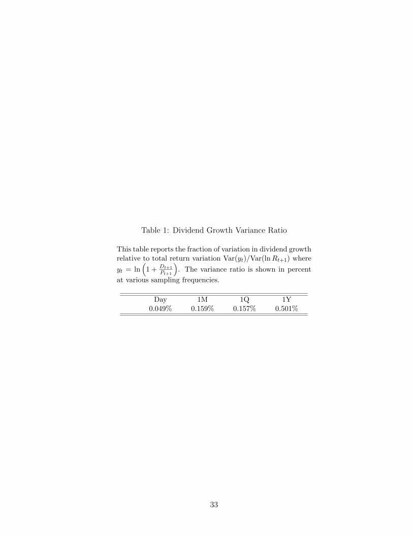
Table 1: Dividend Growth Variance Ratio

This table reports the fraction of variation in dividend growthrelative to total return variation Var(yt)/Var(lnRt+1) where

yt = ln(

1 + Dt+1

Pt+1

). The variance ratio is shown in percent

at various sampling frequencies.

Day 1M 1Q 1Y0.049% 0.159% 0.157% 0.501%

33

Table 2: Predictability of VIX

This table reports the results of the contemporaneous regression rt = A+B4xt +ut for xt = the VIX2

index in Panel A. Panel B reports the autocorrelation (AC) of VIX2, the correlation between h periodahead returns and current VIX2, and test statistics t1, .., t4 as described in the test.

Panel A: Contemporaneous regression/ correlation

BOLS Corr(rt,4xt)-0.188 -0.713(0.003) (0.011)

Panel B: Predictive relationsHorizon AC Corr(rt+i, xt) t1 t2 t3 t4

1 0.965 0.019 -5.681 -5.681 0.0003 0.928 0.020 -5.197 -3.523 -0.481 -0.1424 0.910 0.020 -4.871 -3.119 -0.533 -0.1785 0.901 0.014 -5.251 -3.042 -0.779 -0.33210 0.862 0.006 -5.761 -2.583 -1.062 -0.41922 0.727 0.010 -5.103 -2.494 -0.914 -0.38644 0.502 0.041 -4.232 -2.474 -0.441 -0.08566 0.409 0.016 -3.684 -2.351 -0.612 -0.342132 0.158 0.145 -1.914 -1.261 1.552 1.684252 0.058 0.211 0.399 0.573 2.778 2.813

34

Table 3: Predictability of RV

This table reports the results of the contemporaneous regression rt = A+B4xt+ut for xt = the RealizedVariance (RV) computed from one day intraday returns in Panel A. Panel B reports the autocorrelation(AC) of RV, the correlation between h period ahead returns and current RV, and test statistics t1, .., t4as described in the test.


BOLS Corr(rt,4xt)-0.001 -0.127(0.000) (0.016)


1 0.649 0.050 -0.168 -0.1683 0.522 0.022 -1.501 -0.741 -1.373 -0.6574 0.566 0.017 -1.293 -0.479 -1.194 -0.4275 0.529 0.016 -1.370 -0.521 -1.265 -0.46510 0.445 -0.006 -1.205 -0.731 -1.142 -0.69622 0.363 -0.029 -0.985 -0.782 -0.953 -0.76144 0.179 -0.012 -0.580 -0.508 -0.557 -0.48966 0.152 -0.048 -0.864 -0.822 -0.848 -0.809132 0.044 0.039 0.452 0.464 0.468 0.479252 0.033 0.086 1.312 1.318 1.322 1.328

35

Table 4: Predictability of VRP

This table reports the results of the contemporaneous regression rt = A + B4xt + ut for xt = varianceRisk Premium (VRP). The VRP is computed by taking the difference between squared VIX and onemonth lagged RV. Panel A reports the contemporaneous relationship between changes in VRP andreturns. Panel B reports the autocorrelation (AC) of RV, the correlation between h period aheadreturns and current RV, and test statistics t1, .., t4 as described in the text.


BOLS Corr(rt,4xt)-8.510 -0.721(0.113) (0.010)


1 0.856 0.080 -6.155 -6.155 0.0003 0.671 0.124 -9.457 -7.647 -0.184 0.5644 0.590 0.132 -10.879 -8.869 -0.370 0.4605 0.546 0.129 -13.016 -9.788 -1.059 0.27510 0.363 0.142 -11.754 -8.217 -0.943 0.51922 0.159 0.151 -7.483 -5.697 0.572 1.31044 0.164 0.212 -0.850 0.129 2.678 3.08266 0.208 0.250 0.891 1.710 3.199 3.537132 0.148 0.230 1.862 2.254 3.415 3.577252 0.136 0.174 1.308 1.516 2.203 2.289

36

Table 5: Predictability of VRP II

This table reports the results of the contemporaneous regression rt = A + B4xt + ut for xt = varianceRisk Premium (VRP). The VRP is computed by taking the difference between squared VIX and aforecast of next month’s RV. Panel A reports the contemporaneous relationship between changes inVRP and returns. Panel B reports the autocorrelation (AC) of RV, the correlation between h periodahead returns and current RV, and test statistics t1, .., t4 as described in the text.


BOLS Corr(rt,4xt)-3.433 -0.252(0.183) (0.013)


1 0.872 0.026 -3.597 -3.597 0.0003 0.815 0.062 -3.135 0.373 1.462 2.8964 0.790 0.069 -2.905 0.759 1.424 2.9225 0.774 0.065 -3.072 0.541 0.859 2.33610 0.717 0.090 -2.219 1.806 1.623 3.26822 0.682 0.107 -0.350 1.727 1.494 2.34344 0.568 0.150 0.928 1.742 1.777 2.11066 0.497 0.174 1.199 1.657 1.744 1.931132 0.300 0.245 2.785 2.998 3.205 3.292252 0.207 0.229 2.322 2.407 2.566 2.601

37

Table 6: Predictability of Default Premium

This table reports the results of the contemporaneous regression rt = A + B4xt + ut for xt = defaultpremium (DP). The spread is computed by taking the difference between bonds with BAA and AAAMoodys ratings. Panel A reports the contemporaneous relationship between changes in DS and returns.Panel B reports the autocorrelation (AC) of DS, the correlation between h period ahead returns andcurrent DS, and test statistics t1, .., t4 as described in the text.


BOLS Corr(rt,4xt)-0.001 -0.010(0.004) (0.032)


1 0.980 0.050 1.370 1.370 0.0002 0.947 0.065 1.348 1.338 -0.094 -0.5493 0.917 0.081 1.417 1.406 -0.027 -0.5816 0.827 0.117 1.690 1.675 0.119 -0.66412 0.654 0.164 1.849 1.829 0.237 -0.71524 0.368 0.153 1.580 1.555 -0.373 -1.60436 0.212 0.154 1.574 1.551 -0.726 -1.90548 0.213 0.171 1.590 1.579 -0.656 -1.23660 0.299 0.199 1.645 1.645 -0.345 -0.32072 0.303 0.160 1.168 1.171 -0.618 -0.437

38

Table 7: Predictability of TBill levels

This table reports the results of the contemporaneous regression rt = A + B4xt + ut for xt = 3 monthTBILL rate. Panel A reports the contemporaneous relationship between changes in TBILL and returns.Panel B reports the autocorrelation (AC) of TBILL, the correlation between h month ahead returnsand current TBILL, and test statistics t1, .., t4 as described in the text.


BOLS Corr(rt,4xt)-0.013 -0.106(0.004) (0.032)


1 0.993 -0.071 -2.410 -2.410 0.0002 0.982 -0.090 -2.225 -2.290 0.165 0.9163 0.972 -0.106 -2.151 -2.228 0.202 1.0966 0.944 -0.135 -2.093 -2.174 0.320 1.25312 0.896 -0.171 -1.954 -2.020 0.468 1.23824 0.783 -0.204 -2.116 -2.228 0.944 2.24736 0.708 -0.249 -2.546 -2.656 1.268 2.54548 0.672 -0.275 -2.499 -2.559 1.362 2.05360 0.662 -0.281 -2.274 -2.281 1.366 1.44472 0.640 -0.282 -2.282 -2.264 1.599 1.396

39

Table 8: Predictability of Term Structure Slope

This table reports the results of the contemporaneous regression rt = A + B4xt + ut for xt = termstructure slope. The slope is defined as the difference between 10 and 1 year yield on Treasuries. PanelA reports the contemporaneous relationship between changes in Slope and returns. Panel B reports theautocorrelation (AC) of Slope, the correlation between h period ahead returns and current Slope, andtest statistics t1, .., t4 as described in the text.


BOLS Corr(rt,4xt)0.018 0.110

(0.006) (0.036)


1 0.972 0.089 2.712 2.712 0.0002 0.926 0.110 2.561 2.672 -0.182 -0.9293 0.886 0.128 2.433 2.564 -0.233 -1.1196 0.779 0.155 2.497 2.644 -0.424 -1.41612 0.589 0.218 2.784 2.943 -0.263 -1.33524 0.210 0.265 3.443 3.735 -0.444 -2.41436 -0.064 0.359 4.921 5.317 0.179 -2.49548 -0.074 0.397 4.418 4.646 0.335 -1.20360 0.090 0.371 3.092 3.133 0.123 -0.15272 0.165 0.330 2.349 2.335 -0.155 -0.056

40

Documents

Predictability Puzzles - Marginal Qeraker.marginalq.com/predPuzzles.pdf · Predictability Puzzles Bj˝rn Eraker March 19, 2017 ... is, the equilibrium log price-dividend ratio is