On limited Predictability

By A . WIIN-NIELSEN

Matematisk-fysiske Meddelelser 47

Det Kongelige Danske Videnskabernes SelskabThe Royal Danish Academy of Sciences and Letters

Abstract

The limited predictability experienced by extended integrations of the nonlinear equations governing alarge class of systems is illustrated by a number of examples . Lacking a general theory permitting an es-timate of the limits of the predictability for a given system the strategy is to compare two numerical in-tegrations starting either from slightly different initial states or from identical initial states, but wit hsmall changes in the forcing .

The difference between the practical and the theoretical limits of predicitability is discussed . The the-oretical limit may be determined by starting from two initial states with only infinitesimal differences o rfrom similar differences in the forcing, while the practical limit is determined by the uncertainty of th einitial state due to the accuracy and distributions of observations and by the uncertainty in describing theforcing of a given system.

By A. Wiin-Nielse nNiels Bohr Institute for Astronomy, Physics and Geophysic s

Department of Geophysic sJuliane Maries Vej 3 0

2100 Copenhagen, Denmark .

© Det Kongelige Danske Videnskabernes Selskab 199 9Printed in Denmark by Special-Trykkeriet Viborg a- s

ISSN 0023-3323 . ISBN 87-7304-185-8

1 . Introductio n

The equations of classical physics are deterministic providing one and only one so-lution for a given initial state and a given forcing . The independent variables ar enormally three space coordinates and one time coordinate . The dependent variablesare in general the three components of the velocity, the pressure, the density and th etemperature, but in many cases a reduced set of independent and dependent vari-ables have been used . The solution of the classical two-body astronomical proble mrequires only the basic Newtonian law that mass times acceleration is equal to th esum of forces acting on the mass . Geophysical modeling has also developed overseveral decades, going from the simple to the more complicated . In some cases it i snecessary to supplement the basic six dependent variables by additional variable sbecause the system under consideration may require special treatment of one of it scomponents . As an example it may be mentioned that a realistic treatment of the at -mosphere of the Earth requires a special equation for the content of water vapour .Otherwise it is not possible to treat the cloud and precipitation processes .

From the times of Newton to about 1890 it was generally believed that if oneknows the initial state with great accuracy, and if all the forces acting on a give nsystem can be formulated with equal accuracy, it would be possiple, in principle, t omake predictions of the state of the universe for an infinitely long time .

The limited predictability of physical systems has been known for about a cen-tury. The first discussion of the concept, known by the author, was given b yPoincaré (1893 and 1912) . He discussed in particular the limited predictability inthe three body astronomical problem indicating that small changes in the initia lstate could result in large changes in the trajectories of the three bodies during th enumerical integration of the three relevant equations . A single example of such anintegration is presented in the appendix to this paper .

The best known example of both theoretical and operational limited predictabil-ity is the weather prediction problem simply because objective numerical weathe rpredictions using various models based on the atmospheric dynamics have been i noperation for almost half a century. Thompson (1957) was the first to analyse th elimited predictability due to the uncertainties in the initial field . Since these predic-

4

MfM 47

tions have been verified for a long time it has been possible to follow the gradualincrease of the operational predictability from a single to several days . Within th efield of weather predictions we have also some estimates of the theoretical limit o fpredictability . The weather prediction problem will be discussed in Section 2 of thi spaper .

In other geophysical areas we have much less information about predictability .The reason is of course that no other area has experienced the same systematic de-velopment and use of observational systems for predictions as has been the case i nthe atmospheric sciences . On the other hand, atmospheric prediction models hav ebeen developed to a state where information about the upper layers of the oceans ,the distribution of land and sea ice, the topography and the vegetation of the conti-nents are necessary for a proper determination of the initial state for an atmospher-ic prediction and for the interactive processes during the numerical integration o fthe model equations . Chaos is equivalent to limited predictability simply becaus echaos is defined as sensitivity to small changes in the initial state .

The predictions mentioned so far are attempts to forecast a future state in a smuch detail as possible . The numerical integrations may be based on a grid-poin tmodel, a spectral model or a combination of the two in the sense that a spectra lmodel is used for the time integrations, while a grid-point model is used to deter -mine the influence of local processes on the forcing of the model . The reason forsuch an arrangement is that the spectral equations may be integrated with great ac -curacy, but to incorporate processes on a small scale at a given locality it is neces-sary to know local changes with great accuracy. In the latter case it is necessary t ohave effective and accurate programs to go back and forth between the two kinds o frepresentation. Such programs, depending on fast Fourier transforms, have bee ndeveloped .

A second kind of desirable prediction is to predict a future averaged state of asystem. The goals could for example be to make monthly predictions, seasonal pre -dictions or simulations of various climatic states . A direct approach to this proble mis to integrate a suitable model for a sufficiently long time whereafter the appropri-ate time average is computed as the end product . In view of the limited predictabil-ity one may ask if this procedure will lead to a suitable and useful prediction . It i sof course realized that the transient, relatively short waves after such a long inte -gration will not be found in the correct place and with a suitable amplitude .However, the time average will to a large extent eliminate the transient waves an dthe final product should thus in addition to the zonal state contain mainly the verylong waves which are forced by the topography and the heat sources . If this argu-ment is correct, it may be asked if one could not just as well use a spectral modelcontaining only components describing the smaller wave numbers, i .e . the larg eplanetary scales . This possibility requires that the shorter transient waves do not

MfM 47

5

feed energy into the longer waves, but diagnostic studies of the energy transfers i nthe spectral domain conducted by Lin and Derome (1995) indicates that the largestscale waves do indeed receive energy from the shorter transient waves indicatingthat a lower order model, treating only the large planetary scales, is not a viablepossibility. A second possibility is to avoid the major nonlinear terms by averagin gthe equations over the whole globe . The major nonlinear terms average to zero i nthis case, and the remaining equations are much easier to handle . The disadvantageof this procedure is that one will also have to deal with the physical processes in a naverage way. It is thus not possible to pay attention to size and position of the con-tinents and the oceans . However, this approach may be used as a supplement to th every long integrations of the original equations for the model . Thus, the problemsof predictions of the second kind has not so far been solved in a satisfactory way.

The determination of the practical limit for atmospheric predictability requires alarge number of cases of global integrations . Reliable results can be obtained onlyfrom institutions engaged in the production of such forecasts . To illustrate limitedpredictability it is possible to select various low order models and use the integra-tions of the model equations to demonstrate the main nature of the phenomenon .Since these model contain only a few components, they will not be able to pay at-tention to the nonlinear cascades of energy in the spectrum . Some low-order mod -els will be defined and used in Section 3 of this paper.

2 . Atmospheric prediction s

Atmospheric predictions were for a long time based on the experience of the fore-caster and on empirical and statistical rules . Such forecasts were normally limite dto 1 or 2 days . With the availability of the first computers appearing in the late1940's it became possible for the first time to attempt atmospheric forecasts base don simple models of the dynamics of the atmosphere . The very first model, formu-lated in 1949, used the vorticity equation applied to the vertically averaged atmos-phere . This simple barotropic model assuming quasi-geostrophic or quasi-non-divergent flow was later replaced by models using several levels to describe th evertical structure of the atmosphere . The first models had neither energy source snor dissipation. They could generally be used for a couple of days and were ofte nintegrated on grids covering less than a hemisphere .

These models were later replaced by more complete hemispheric and globa lmodels using the primitive equations . A description of the general development ha sbeen given by the author (Wiin-Nielsen, 1997) . Present models for short- an dmedium-range prediction are typically global with a large number of levels to de -scribe the vertical variations of the atmosphere . The best models has a horizontal

6

MfM 47

resolution permitting wavelengths as small as 200 km. The models contain heatsources and sinks as well as friction in the boundary layer and the free atmosphere .The radiation budgets for the incoming short wave radiation and the outgoing lon gwave radiation are a part of the model . The orography is included with a resolutio ncorresponding to the horizontal resolution of the model . Special quantities are nec-essary at the surface such as ground and sea roughness, ground and sea surfac etemperatures, ground humidity, snow-cover and sea ice . Gravity wave drag, evapo-ration, transfer of sensible and latent heat flux are included . The clouds are dividedin high, medium, low and convective clouds . One deals with both stratiform andconvective precipitation as well as an almost complete water budget at the surfac eand sub-surface levels .

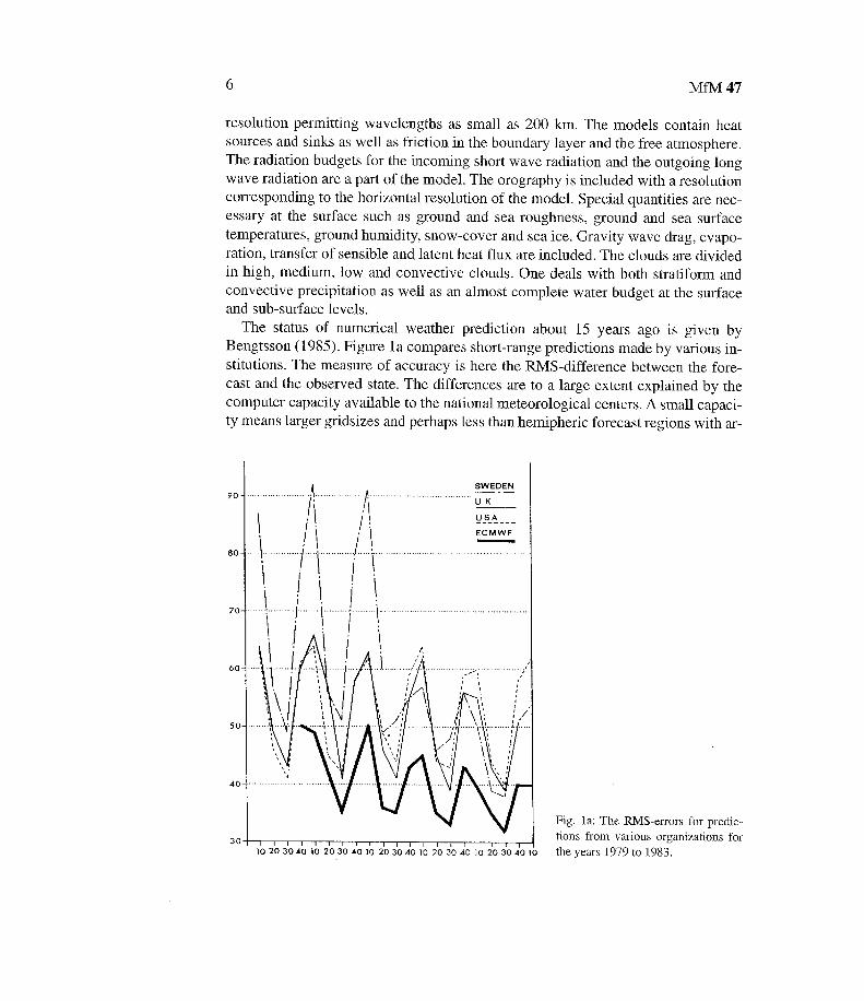
The status of numerical weather prediction about 15 years ago is given b yBengtsson (1985) . Figure la compares short-range predictions made by various in-stitutions . The measure of accuracy is here the RMS-difference between the fore -cast and the observed state . The differences are to a large extent explained by th ecomputer capacity available to the national meteorological centers . A small capaci-ty means larger gridsizes and perhaps less than hemipheric forecast regions with ar -

Fig . la : The RMS-errors for predic-tions from various organizations forthe years 1979 to 1983 .

MfM 47 7

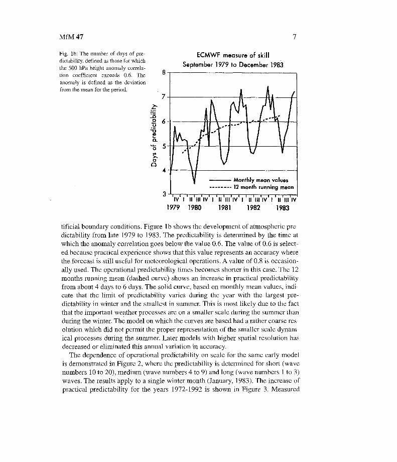
Fig . lb: The number of days of pre-dictability, defined as those for whic hthe 500 hPa height anomaly correla-tion coefficient exceeds 0 .6 . Theanomaly is defined as the deviatio nfrom the mean for the period .

8

ECMWF measure of skil lSeptember 1979 to December 1983

A!'

mean value sMonthly 12 month running mean

tificial boundary conditions . Figure lb shows the development of atmospheric pre-dictability from late 1979 to 1983 . The predictability is determined by the time a twhich the anomaly correlation goes below the value 0 .6 . The value of 0 .6 is select -ed because practical experience shows that this value represents an accuracy wher ethe forecast is still useful for meteorological operations . A value of 0 .8 is occasion -ally used. The operational predictability times becomes shorter in this case . The 1 2months running mean (dashed curve) shows an increase in practical predictabilit yfrom about 4 days to 6 days . The solid curve, based on monthly mean values, indi-cate that the limit of predictability varies during the year with the largest pre-dictability in winter and the smallest in summer . This is most likely due to the factthat the important weather processes are on a smaller scale during the summer tha nduring the winter. The model on which the curves are based had a rather coarse res -olution which did not permit the proper representation of the smaller scale dynam-ical processes during the summer. Later models with higher spatial resolution ha sdecreased or eliminated this annual variation in accuracy .

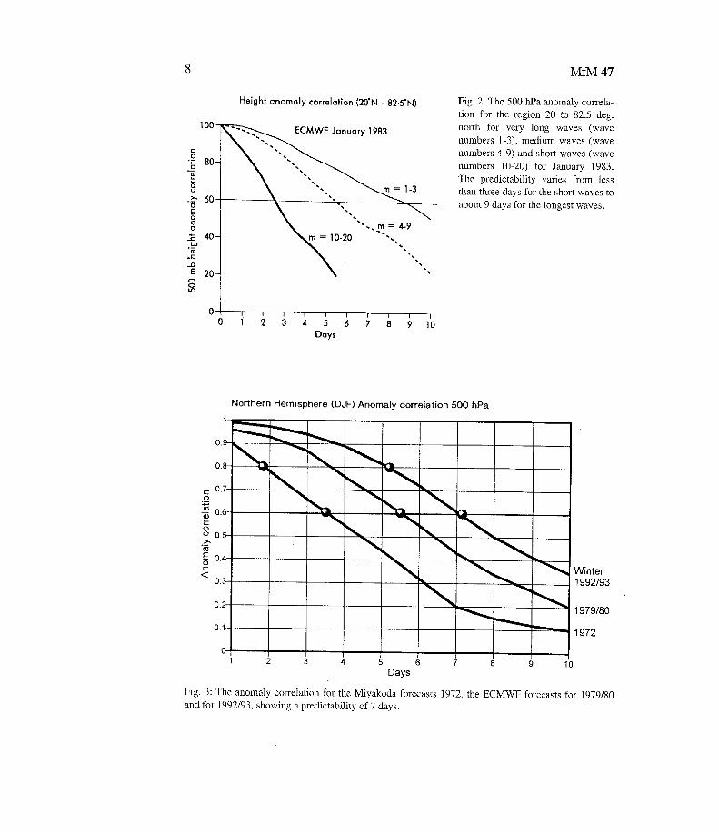
The dependence of operational predictability on scale for the same early mode lis demonstrated in Figure 2, where the predictability is determined for short (wav enumbers 10 to 20), medium (wave numbers 4 to 9) and long (wave numbers 1 to 3 )waves . The results apply to a single winter month (January, 1983) . The increase ofpractical predictability for the years 1972-1992 is shown in Figure 3 . Measure d

6 -

S

4

3

f

1IV 1

II III IV I

II III IV I

II Ill IV I

II III

IV

1979 1980

1981

1982

1983

8 MfM 47

Height anomaly correlation (20°N - 82 .5°N) Fig . 2: The 500 hPa anomaly correla-tion for the region 20 to 82 .5 deg .north for very long waves (wavenumbers I-3), medium waves (wavenumbers 4-9) and short waves (wavenumbers 10-20) for January 1983 .The predictability varies from lessthan three days for the short waves t oabout 9 days for the longest waves .

Northern Hemisphere (DJF) Anomaly correlation 500 hP a1

~'~\i'̀-~ô

07

M-~ o . 11I .w111 .wO.T p .

111 .11M-I.E 0 . 4

o

sWI\

0 .1

01

2

3

4

5

6

7

8

9

1 0Days

Fig . 3 : The anomaly correlation for the Miyakoda forecasts 1972, the ECMWF forecasts for 1979/8 0and for 1992/93, showing a predictability of 7 days .

0 . 2

.

`

0 .

0 .

Winte r1992/93

1979/80

1972

Tendency correlation coefficient from 1968 to 1992 for forecasts of msl pArea : North Atlantic and Europ e

1 .0 o24-hr forecast48-hr forecas t72-hr forecas t96-hr forecas t

5-

0 . 9Co

0. 8a)

0 . 7

0 .6

_AM mod _

_VfAirmallaTaii/M111

0 .9

o

5-

0 .6 01968 1970 1972 1974 1976 1978 1980 1982 1984 1986 1988 1990 199 2

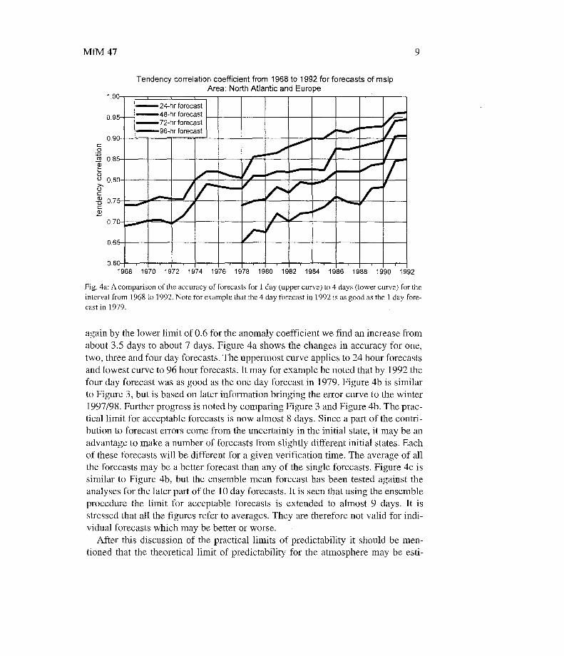
Fig . 4a : A comparison of the accuracy of forecasts for 1 day (upper curve) to 4 days (lower curve) for th einterval from 1968 to 1992. Note for example that the 4 day forecast in 1992 is as good as the 1 day fore -cast in 1979 .

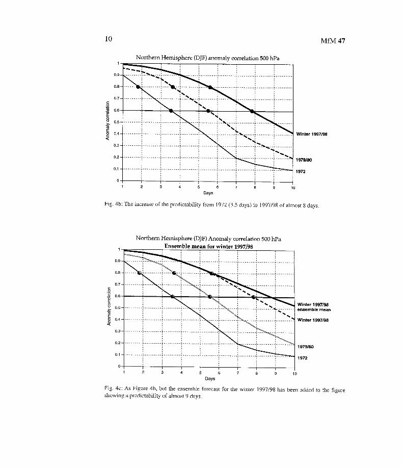
again by the lower limit of 0 .6 for the anomaly coefficient we find an increase fro mabout 3 .5 days to about 7 days . Figure 4a shows the changes in accuracy for one ,two, three and four day forecasts . The uppermost curve applies to 24 hour forecast sand lowest curve to 96 hour forecasts . It may for example be noted that by 1992 th efour day forecast was as good as the one day forecast in 1979 . Figure 4b is similarto Figure 3, but is based on later information bringing the error curve to the winte r1997/98 . Further progress is noted by comparing Figure 3 and Figure 4b . The prac-tical limit for acceptable forecasts is now almost 8 days . Since a part of the contri-bution to forecast errors come from the uncertainty in the initial state, it may be anadvantage to make a number of forecasts from slightly different initial states . Eachof these forecasts will be different for a given verification time . The average of al lthe forecasts may be a better forecast than any of the single forecasts . Figure 4c i ssimilar to Figure 4b, but the ensemble mean forecast has been tested against th eanalyses for the later part of the 10 day forecasts . It is seen that using the ensembleprocedure the limit for acceptable forecasts is extended to almost 9 days. It i sstressed that all the figures refer to averages . They are therefore not valid for indi-vidual forecasts which may be better or worse .

After this discussion of the practical limits of predictability it should be men-tioned that the theoretical limit of predictability for the atmosphere may be esti-

10

MfM 47

Northern Hemisphere (DJF) anomaly correlation 500 hPa

Winter 1997/98

1979/80

1972

3

4

5

6

7Days

Fig . 4b : The increase of the predictability from 1972 (3 .5 days) to 1997/98 of almost 8 days .

Northern Hemisphere (DJF) Anomaly correlation 500 hPaEnsemble mean for winter 1997/9 8

0. 9

0. 8

0. 7

0. 6

0. 5

0 . 4

0 . 3

0 .2

0 .1

o

'•• ---- . .-•^v`

`

.

. . .`~%4, ♦

~t `

rs,

~t : . . . . . . .

t. .` ,

.

,- ----------------- - ----- - 1,..`

,

.

.

•.

.

..

.

..

.

,

,

.

. . .

" %.. . . .

. . . . . .

. . . . . ...

.

,

`

2 8 9 1 0

9

1 0Days

Fig. 4c : As Figure 4b, but the ensemble forecast for the winter 1997/98 has been adde dshowing a predictability of almost 9 days .

to the figure

MfM 47

1 I .

mated by making two long integrations starting from initial states which are almos tidentical . The initial states differ only by infinitesimal amounts . The problem i sthus to determine when the difference between the two integrations become toolarge . The first attempts were made as early as 1966 as part of the preparation fo rthe Global Weather Experiment (Charney, 1966) . Such experiments are not easy t ocarry out . The initial difference was introduced in the temperature fields as a singlewave component in the baroclinically unstable region . Three different models wereused . If the difference between the two initial states is very small, the dissipation inthe model will have a tendency to eliminate the difference . One of the models gaveindeed the result that the difference between the two forecasts increased in th eearly part of the integration, but decreased then to small values . Nevertheless, a cer -tain estimate was made based on one of the models, and the result was a theoretica llimit of predictability of 15 to 19 days . Since then models have become better bot hwith respect to the parameterization of the physical processes and the vertical an dhorizontal resolution. It may be worthwhile to attempt a new determination of th etheoretical limit of predictability using the best global models .

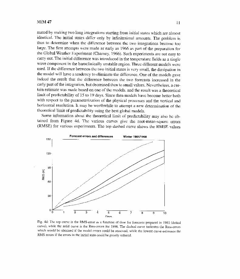
Some information about the theoretical limit of predictability may also be ob-tained from Figure 4d . The various curves give the root-mean-square errors(RMSE) for various experiments . The top dashed curve shows the RMSE values

1 0

Fig . 4d : The top curve is the RMS-error as a function of time for forecasts prepared in 1981 (dotte dcurve), while the solid curve is the Rms-errors for 1998 . The dashed curve indicates the Rms-error swhich would be obtained if the model errors could be removed, while the lowest curve estimates th eRMS-errors if the errors in the initial state could be greatly reduced .

12

MfM 47

for the winter 1980/81 as a function of time measured in days . The solid curve i sthe RMSE values for the winter 1997/98 indicating the improvements of the fore-casts over 17 years of operational predictions . The third (dashed) curve from th etop is obtained by removing the model errors beyond Day 1 . It shows in otherwords the potential skill, if the model was perfect, while the forecasts still are in-fluenced by the uncertainty in the initial state . The lowest (dashed-dotted) curve in-dicates the potential skill if the erorrs at day 1 was further reduced by as much asthe reduction experienced from 1980/81 to 1997/98 . If such an improvement coul dbe obtained a further extention of the operational predictability would be possible .In this imagined situation even the 10 day forecasts would be useful .

The curves in Figure 4d are limited to 10 days because the daily operational fore -casts are not carried beyond this time. A theoretical limit of predictability could beobtained if the forecasts on an experimental basis were carried so far into the futur ethat the three lowest curves converged . Such experiments may be carried out in thefuture .

The reason for the present operational limit of predictability is that the observa-tions do not permit an initial analysis without errors . In addition, the description o fthe many physical processes in the atmosphere necessary to determine the net heat -ing is done by parameterizing small scale processes in terms of the gridpoint vari-ables used in the model . Such a process cannot be without errors since it depend son empirical and statistical procedures . It is most likely that the latest gain in oper-ational predictability is due to better atmospheric observations, particularly the in -formation from satellites, because the improvements are seen also for the forecast sfor the shorter periods .

3 . Limited predictability in simple geophysical model s

Since no general theory is known for limited predictability it will be necessary to il -lustrate the behavior by selecting various examples . They will be based on low-or-der models where the integrations can be carried out with ease . Low-order model shave limitations . They contain the nonlinear interactions among the spectral com-ponents in a rudimentary form only. Therefore, they do not have cascade processe slinking the spectral region of the large-scale forcing with the dissipation range .Nevertheless, they are convenient tools that can illustrate the occasionally unex-pected behavior due to the nonlinear nature of the models .

Example A : Lorenz attractorWe select the well known strange Lorenz attractor as the first example . It has beendescribed in many references such as Lorenz (1963, 1989) . The equations for the

MfM 47

1 3

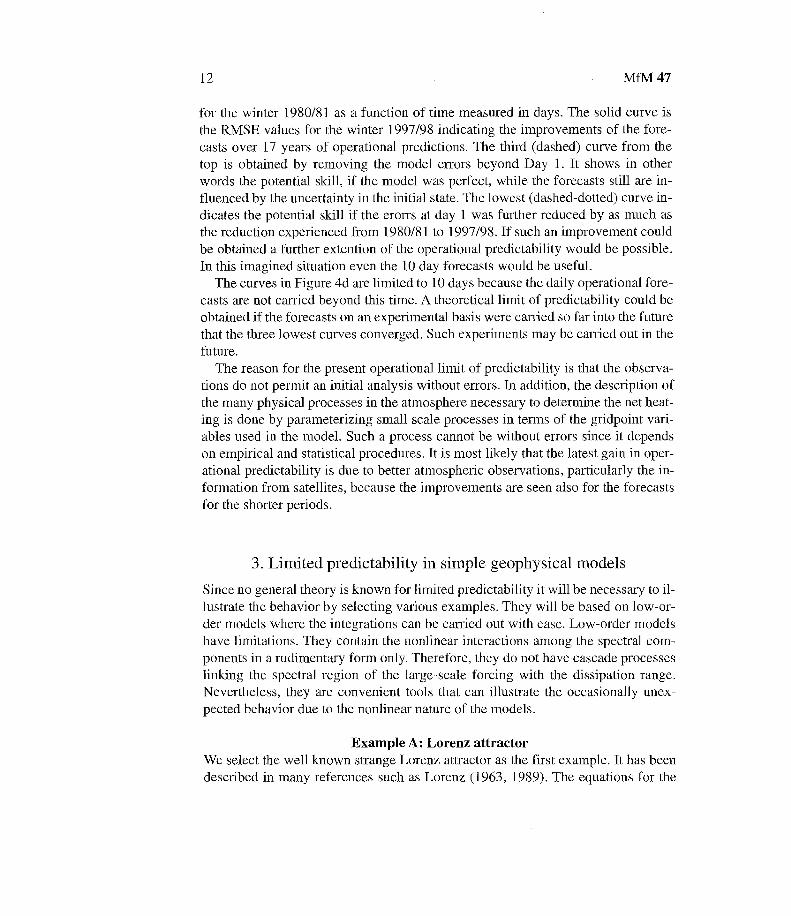
model are given in (3 .1) using the standard notations . We recall that the model de-cribes convection between two horizontal plates .

dx =6(y-x )

dt

dy= xz+rxy

dz = xy-bzdt

The standard case will be used. It has b=813 and 6=10. r is the Rayleigh number,and it is proportional to the temperature difference between the lower and the uppe rhorizontal plates . The theory for the convection says that if r<1 we get moleculartransfer of heat from the lower to the upper plate . For r>1, but not too large, con-vection cells develop between the plates . When 1<r<rc (re = 24 .74) the equation shave one unstable state (0,0,0) and two steady states, while r>re results in three un -stable steady states . In the latter case the system will never come to rest . On the oth -er hand, it can be shown that the system cannot go to infinity because being suffi-ciently far away from (0,0,0) it will move back towards this point .

We select first r=28 . It is in the region containing three unstable steady state . Anintegration from a given initial state is carried out . A second integration with r, =28 .001 from the same initial state is included in the program. Let the variables inthe second integration be denoted (u,v,w) . As a measure of the difference betwee nthe two integration we may use the rms-value given in (3 .2) .

d= [(x-u)2-1-(y-v)2+(z-w)z] i'z

(3 .2 )

With a starting position for both integrations in (0,0 .01,0) integrations were carrie dout for 40 time units . The difference as measured by (3 .2) is shown in Figure 5 .Between 20 and 25 time units we notice that the two solutions are definitely differ -ent . The difference between them changes in time, but the two solutions do no tcome close to each other again .

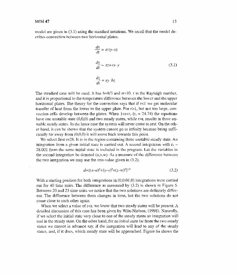
When we select a value of r<r~ we know that two steady states will be present . Adetailed discussion of this case has been given by Wiin-Nielsen, (1998) . Naturally,if we select the initial state very close to one of the steady states an integration wil lend in the steady state . On the other hand, for an initial state far from the two stead ystates we cannot in advance say, if the integration will lead to any of the stead ystates, and, if it does, which steady state will be approached . Figure 6a shows th e

(3 .1)

14

MfM 47

r=28 .0,r1 =28.001,xo=u0=0,y=v=0 .01, z=w= 050

45

40 -

~ (

I I35 -

~

30

25-o20

4 s15 -

b ~

10

5 -

\,

0

5

10

15

20

25

30

35

40t

Fig. 5 : The RMS-difference between two integrations of the Lorenz-model if the forcing is changed b y0 .001 . The predictability is lost between 20 and 25 time units .

r=23 . 0 , r1 =23 .0000001,xo=uo=0,yo=vo=0.1,zo=w0=23 . 0

-o

10

5

100

200

300

400

500

600

700t

Fig . 6a : The stable part of the Lorenz attractor . Two integrations from the same initial states, but th eforcing is changed by 10' . The two integrations arrive in different steady states .

MfM 47 1 5

r=23 . 0 ,r1 =23.0000001,xo =uo=0,yo=vo=0.1,zo=w0=23 . 0

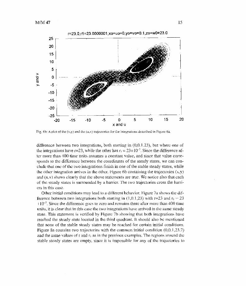
Fig . 6b : A plot of the (x,y) and the (u,v) trajectories for the integrations described in Figure 6a .

difference between two integrations, both starting in (0,0 .1,23), but where one o fthe integrations have r=23, while the other has r, = 23+10' . Since the difference af-ter more than 400 time units assumes a constant value, and since that value corre-sponds to the difference between the coordinates of the steady states, we can con-clude that one of the two integrations finish in one of the stable steady states, whil ethe other integration arrives in the other. Figure 6b containing the trajectories (x,y )and (u,v) shows clearly that the above statements are true . We notice also that eachof the steady states is surrounded by a barrier . The two trajectories cross the barri-ers in this case .

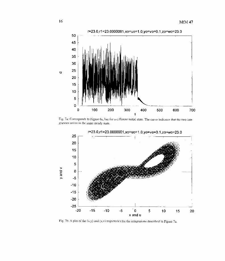
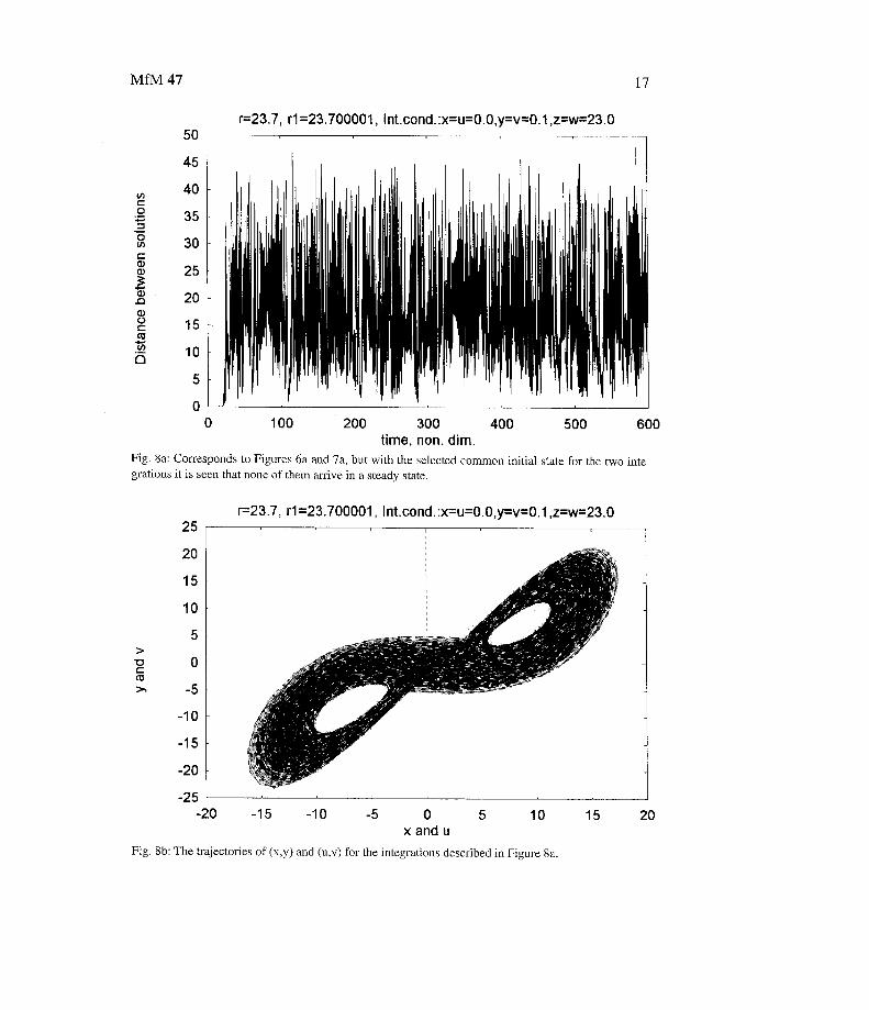
Other initial conditions may lead to a different behavior . Figure 7a shows the dif-ference between two integrations both starting in (1,0 .1,23) with r=23 and r, = 23+10' . Since the difference goes to zero and remains there after more than 400 tim eunits, it is clear that in this case the two integrations have arrived in the same stead ystate . This statement is verified by Figure 7b showing that both integrations havereached the steady state located in the third quadrant . It should also be mentionedthat none of the stable steady states may be reached for certain initial conditions .Figure 8a contains two trajectories with the common initial condition (0,0 .1,23 .7 )and the same values of r and r, as in the previous examples . The regions around thestable steady states are empty, since it is impossible for any of the trajectories to

16

MfM 47

r=23 .0,r1=23 .0000001 ,xo=uo=1 .0,yo= vo=0.1,zo=wo=23 . 0

100

200

300

400

500

600

700t

Fig . 7a : Corresponds to Figure 6a, but for a different initial state . The curve indicates that the two inte -grations arrive in the same steady state .

r=23.0,r1 =23.0000001,xo=uo =l .0,yo=vo=0.1,zo=wo=23 . 0

-5

-1 0

-1 5

-20

-25-20

-15

-10

-5

- 0

5

10

15

20x and u

Fig . 7b: A plot of the (x,y) and (u,v) trajectories for the integrations described in Figure 7a .

0

25

20

1 5

10

5

MfM 47 17

r=23.7, r1=23.700001, Int .cond . :x=u=0.0,y=v=0.1,z=w=23 . 0

00

100

200

300

400

500

600time, non. dim .

Fig. 8a: Corresponds to Figures 6a and 7a, but with the selected common initial state for the two inte -grations it is seen that none of them arrive in a steady state .

r=23 .7, r1=23 .700001, Int .cond . :x=u=0 .0,y=v=0 .1,z=w=23 . 0

~-Dcco~

0x and u

Fig . 8b : The trajectories of (x,y) and (u,v) for the integrations described in Figure 8a .

20

18

MfM 47

penetrate the barriers . Figure 8b shows the differences between solutions for thepresent case. It varies after the growth at about 20 time units .

Example B : Equation of motion with Newtonian forcingAs the second example we shall use a simplified form of the first equation of mo-tion as given in (3 .3) .

Su Su+u

7("E-u)St

Sx

The equation is one dimensional in space . The right hand side contains aNewtonian forcing . It may be consider as a geopotential gradient field, constant i ntime, i .e . 7 uE , and a linear dissipation term. (3 .3) is converted into the spectral do -main by adopting the series given in (3 .4) .

Müll

u(t,x) =

u(n, t) sin (nkx)n= 1

/ir ta,

(3 .4)

uE(x) =

uE (n) sin (nkx),I= 1

We have for simplicity selected the boundary conditions that u and uE vanish atboth boundaries . One could also have selected cosine-functions or a combination o fboth trigonometric functions . The series in (3 .4) are inserted in (3 .3) where the onlynonlinear term is the advection term. The result is the equation given in (3 .5) .

du(n)

Iz- 1(n)= 1 /2 E nku (q) u(n+q) -' l2 qku(q) u(n-q)

3 . 5

The derivations necessary to come from (3 .4) to (3 .5) requiring the extensive use ofFourier expansions have been given by Wiin-Nielsen (1999) . It is furthermore anadvantage to non-dimensionalize (3 .5) . k is the basic wave number (k=2m/L) coile -sponding to the total length, L, of the interval . Introducing a scaling on time T=ÿ- 'and on velocity U=(211/k) we may write the basic equation in the form given i n(3 .6) .

(3 .3 )

dtR=1

9=1

MfM 47

1 9

dx(n)= ""ix-n

n-I

dz

~ nx (q) x(n+q) - ~ qx(q) x(n-q) + xE(n) - x(n)

3 . 69= 1

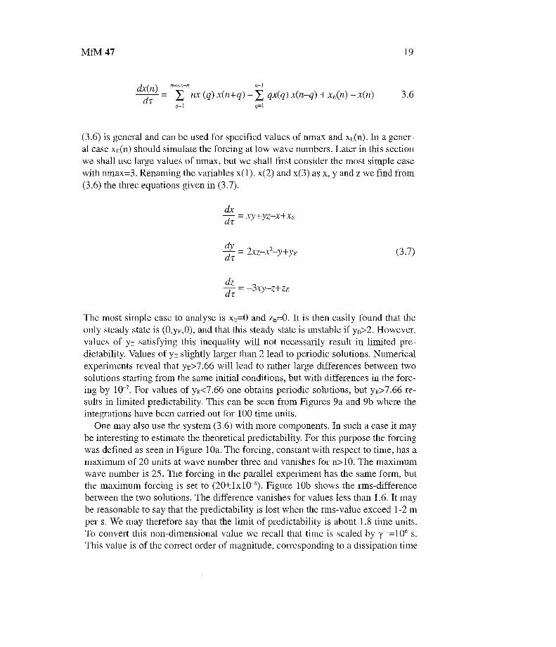
(3 .6) is general and can be used for specified values of nmax and xE(n) . In a gener-al case x E (n) should simulate the forcing at low wave numbers . Later in this sectionwe shall use large values of nmax, but we shall first consider the most simple cas ewith nmax=3 . Renaming the variables x(1), x(2) and x(3) as x, y and z we find fro m(3.6) the three equations given in (3 .7) .

dxcl2- = xy+yz-x+xE

dz = 2xz-x2-y+yE

dz

da-= -3xy-z+zF

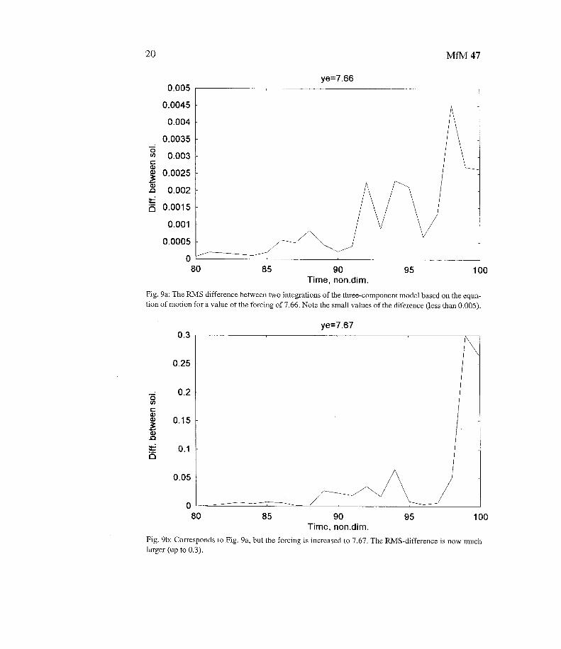
The most simple case to analyse is xE=0 and z E=0 . It is then easily found that th eonly steady state is (O,ye,O), and that this steady state is unstable if ye>2 . However,values of yE satisfying this inequality will not necessarily result in limited pre-dictability. Values of YE slightly larger than 2 lead to periodic solutions . Numerica lexperiments reveal that y E>7 .66 will lead to rather large differences between tw osolutions starting from the same initial conditions, but with differences in the forc-ing by 10' . For values of yE<7.66 one obtains periodic solutions, but yE>7.66 re -sults in limited predictability. This can be seen from Figures 9a and 9b where th eintegrations have been can-ied out for 100 time units .

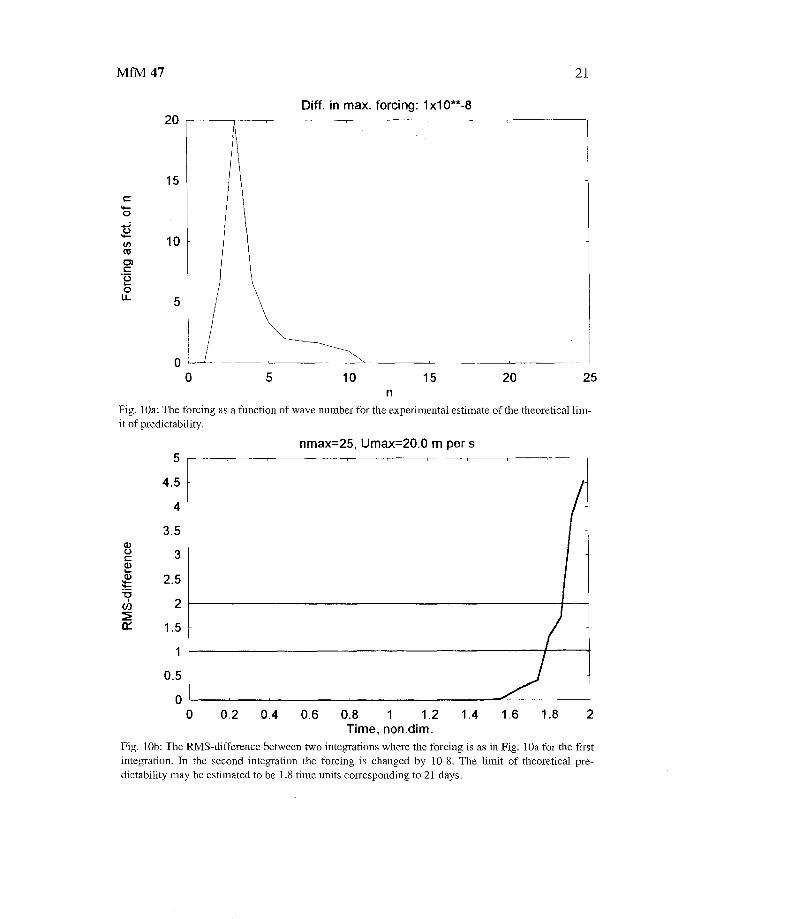
One may also use the system (3 .6) with more components . In such a case it maybe interesting to estimate the theoretical predictability . For this purpose the forcingwas defined as seen in Figure 10a . The forcing, constant with respect to time, has amaximum of 20 units at wave number three and vanishes for n>10 . The maximumwave number is 25 . The forcing in the parallel experiment has the same form, bu tthe maximum forcing is set to (20±1x10-8 ) . Figure 10b shows the rms-differencebetween the two solutions . The difference vanishes for values less than 1 .6 . It ma ybe reasonable to say that the predictability is lost when the rms-value exceed 1-2 mper s . We may therefore say that the limit of predictability is about 1 .8 time units .To convert this non-dimensional value we recall that time is scaled by y- 1 =106 s .This value is of the correct order of magnitude, corresponding to a dissipation tim e

(3 .7)

20

MfM 47

ye=7 .660 .005

0.0045

0.004

0.0035

0.003

0.0025

0.002

0.001 5

0 .00 1

0 .0005

80

85

90

95

100Time, non .dim .

Fig . 9a : The RMS difference between two integrations of the three-component model based on the equa-tion of motion for a value of the forcing of 7 .66 . Note the small values of the diference (less than 0 .005) .

ye=7 .670 . 3

0 .25

0 . 2

0 .1 5

0 . 1

0.05 -

080

85

90

95

100Time, non .dim .

Fig . 9b : Corresponds to Fig . 9a, but the forcing is increased to 7 .67 . The RMS-difference is now muc hlarger (up to 0.3) .

0

MfM 47

2 1

Diff. in max. forcing: 1x10**-820

15

00

5

10

15

20

25n

Fig . 10a : The forcing as a function of wave number for the experimental estimate of the theoretical lim -it of predictability.

nmax=25, Umax=20.0 m per s

0 .2

0 .4

0 .6

0 .8

1

1 .2

1 .4

1 .6

1 .8

2

Time, non .dim .

Fig . 10b : The RMS-difference between two integrations where the forcing is as in Fig . 10a for the firs tintegration. In the second integration the forcing is changed by 10-8 . The limit of theoretical pre-dictability may be estimated to be 1 .8 time units corresponding to 21 days .

5

4 .5

4

3.5

3

2 .5

2

1 . 5

1

0 .5

00

22

MfM 47

of about 10 days, but one could also justify slightly smaller or larger values .Adopting the above value we find that the theoretical limit of predictability is abou t21 days or 3 weeks . It corresponds to an extremely small change in the forcing, bu tassumes an accurate initial condition .

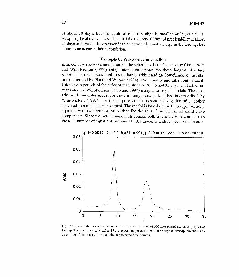
Example C : Wave-wave interactionA model of wave-wave interaction on the sphere has been designed by Christense nand Wiin-Nielsen (1996) using interaction among the three longest planetar ywaves. This model was used to simulate blocking and the low-frequency oscilla-tions described by Plaut and Vautard (1994) . The monthly and intermonthly oscil-lations with periods of the order of magnitude of 70, 45 and 35 days was further in -vestigated by Wiin-Nielsen (1996 and 1997) using a variety of models . The mos tadvanced low-order model for these investigations is described in appendix 1 byWiin-Nielsen (1997) . For the purpose of the present investigation still anotherspherical model has been designed . The model is based on the barotropic vorticit yequation with two components to describe the zonal flow and six spherical wavecomponents . Since the latter components contain both sine and cosine component sthe total number of equations become 14 . The model is with respect to the interac -

g11 =0 .0015,g21 =0 .018,g31 =0.001,g12=0 .0015,g22=0 .018,g32=0.00 10 .06

0 .05

0.04

É 0 .03a

0 .02

0 .01

0

--

0

5

10

15

20

25

30

35n

Fig . l 1 a : The amplitudes of the frequencies over a time interval of 630 days forced exclusively by wav eforcing . The maxima at n=9 and n=18 correspond to periods of 70 and 35 days of atmospheric waves a sdetermined from observational studies for selected time periods .

MfM 47

23

tions a special case of the general spectral barotropic model formulated b yPlatzman (1960) . However, a forcing, constant in time, is added to each equation a swell as a frictional term .

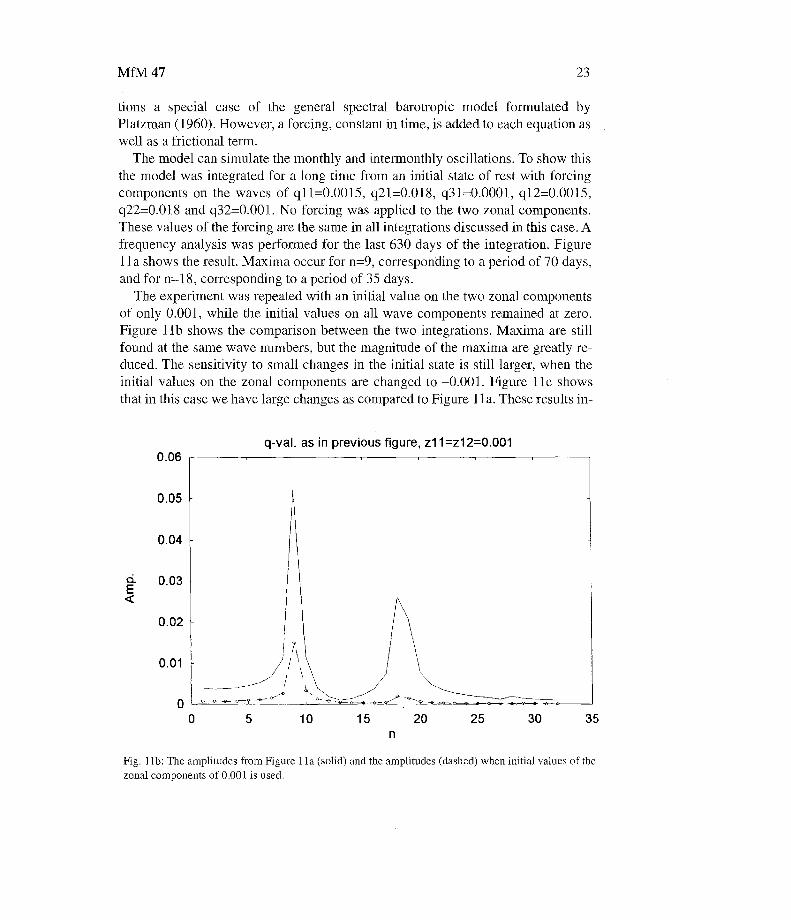
The model can simulate the monthly and intermonthly oscillations . To show thisthe model was integrated for a long time from an initial state of rest with forcin gcomponents on the waves of ql1=0 .0015, q21=0.018, q31=0.0001, q12=0 .0015 ,q22=0.018 and q32=0 .001 . No forcing was applied to the two zonal components .These values of the forcing are the same in all integrations discussed in this case . Afrequency analysis was performed for the last 630 days of the integration . Figure11a shows the result . Maxima occur for n=9, corresponding to a period of 70 days ,and for n=18, corresponding to a period of 35 days .

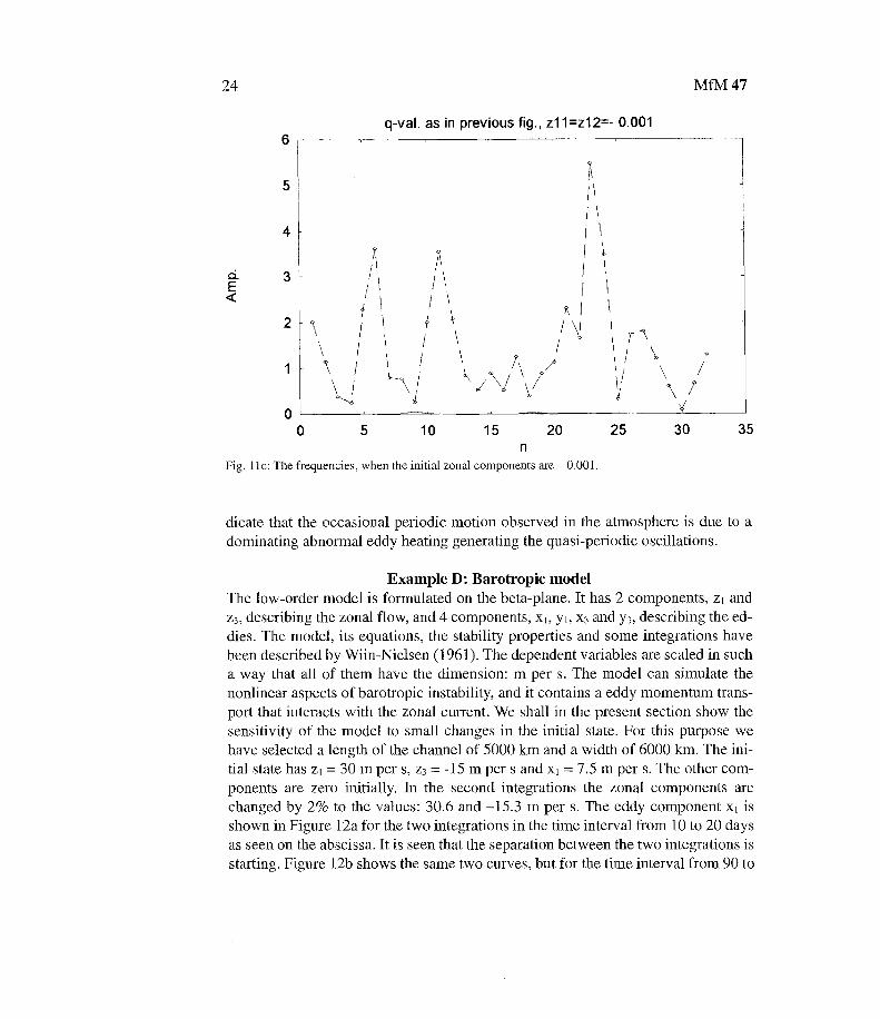
The experiment was repeated with an initial value on the two zonal component sof only 0 .001, while the initial values on all wave components remained at zero .Figure llb shows the comparison between the two integrations . Maxima are stillfound at the same wave numbers, but the magnitude of the maxima are greatly re-duced . The sensitivity to small changes in the initial state is still larger, when th einitial values on the zonal components are changed to -0 .001 . Figure llc show sthat in this case we have large changes as compared to Figure 1 l a. These results in -

0 .06

0 .05

0.04

É

0 .03¢

0.02

0 .01

0

q-val . as in previous figure, z1 1=z12=0 .00 1

0

5

10

15

20

25

30

35n

Fig . l lb : The amplitudes from Figure 1la (solid) and the amplitudes (dashed) when initial values of th ezonal components of 0 .001 is used .

24 MfM 47

q-val . as in previous fig ., z11=z12=- 0 .00 1

I \

1/

1

1 I

II

1Ø ~

I

'\

I

I

Ø

ØI

1\I

~

\~

II

II

1

IØ

7\

/!

11 1

\ I

~~

~~

d1

~ i

nFig . 11c: The frequencies, when the initial zonal components are - 0 .001 .

dicate that the occasional periodic motion observed in the atmosphere is due to adominating abnormal eddy heating generating the quasi-periodic oscillations .

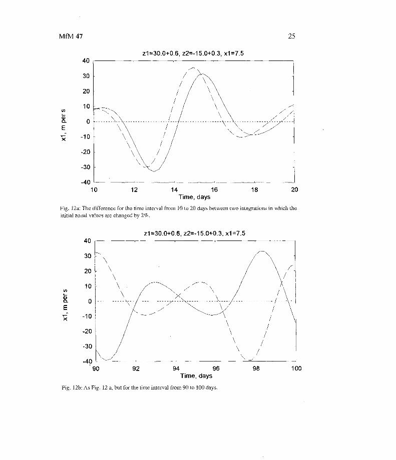
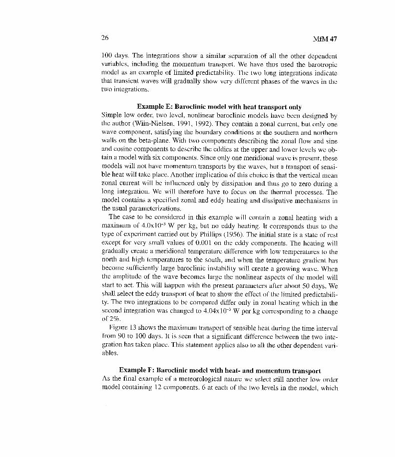
Example D: Barotropic modelThe low-order model is formulated on the beta-plane . It has 2 components, z i andz 3 , describing the zonal flow, and 4 components, x i , y,, x3 and y 3 , describing the ed-dies . The model, its equations, the stability properties and some integrations hav ebeen described by Wiin-Nielsen (1961) . The dependent variables are scaled in suc ha way that all of them have the dimension : m per s . The model can simulate thenonlinear aspects of barotropic instability, and it contains a eddy momentum trans -port that interacts with the zonal current . We shall in the present section show thesensitivity of the model to small changes in the initial state . For this purpose wehave selected a length of the channel of 5000 km and a width of 6000 km . The ini -tial state has z, = 30 to per s, z 3 = -15 m per s and x i = 7 .5 m per s . The other com -ponents are zero initially. In the second integrations the zonal components arechanged by 2% to the values : 30.6 and -15 .3 m per s . The eddy component x, i sshown in Figure 12a for the two integrations in the time interval from 10 to 20 day sas seen on the abscissa . It is seen that the separation between the two integrations i sstarting. Figure 12b shows the same two curves, but for the time interval from 90 t o

6

5

4

3EQ

2

1

00 5 3515 25 3 010 20

MfM 47

25

z1=30 .0+0.6, z2=-15 .0+0.3, x1=7 . 540

30

20

10

0

~

Q.E

X -1 0

-20

\

\

/------ ------- ----------- ----- - -

-30

-4010

12

14

16

18

20Time, days

Fig . 12a : The difference for the time interval from 10 to 20 days between two integrations in which th einitial zonal values are changed by 2% .

z1=30 .0+0 .6, z2=-15 .0+0.3, x1=7 .540

/---- '

-20

-30

-49

w)

;7_E

x

-10\

\

90

92

94

96

98

10 0Time, days

Fig. 12b : As Fig . 12 a, but for the time interval from 90 to 100 days .

26

MfM 47

100 days . The integrations show a similar separation of all the other dependen tvariables, including the momentum transport . We have thus used the barotropicmodel as an example of limited predictability . The two long integrations indicatethat transient waves will gradually show very different phases of the waves in th etwo integrations .

Example E: Baroclinic model with heat transport onl ySimple low order, two level, nonlinear baroclinic models have been designed bythe author (Wiin-Nielsen, 1991, 1992) . They contain a zonal current, but only onewave component, satisfying the boundary conditions at the southern and norther nwalls on the beta-plane . With two components describing the zonal flow and sin eand cosine components to describe the eddies at the upper and lower levels we ob -tain a model with six components . Since only one meridional wave is present, thes emodels will not have momentum transports by the waves, but a transport of sensi-ble heat will take place . Another implication of this choice is that the vertical mea nzonal current will be influenced only by dissipation and thus go to zero during along integration . We will therefore have to focus on the thermal processes . Themodel contains a specified zonal and eddy heating and dissipative mechanisms inthe usual parameterizations .

The case to be considered in this example will contain a zonal heating with amaximum of 4 .0x10-3 W per kg, but no eddy heating . It corresponds thus to th etype of experiment carried out by Phillips (1956) . The initial state is a state of restexcept for very small values of 0 .001 on the eddy components . The heating willgradually create a meridional temperature difference with low temperatures to th enorth and high temperatures to the south, and when the temperature gradient ha sbecome sufficiently large baroclinic instability will create a growing wave . Whenthe amplitude of the wave becomes large the nonlinear aspects of the model wil lstart to act . This will happen with the present parameters after about 50 days . Weshall select the eddy transport of heat to show the effect of the limited predictabili-ty. The two integrations to be compared differ only in zonal heating which in th esecond integration was changed to 4 .04x10 -3 W per kg corresponding to a chang eof 2% .

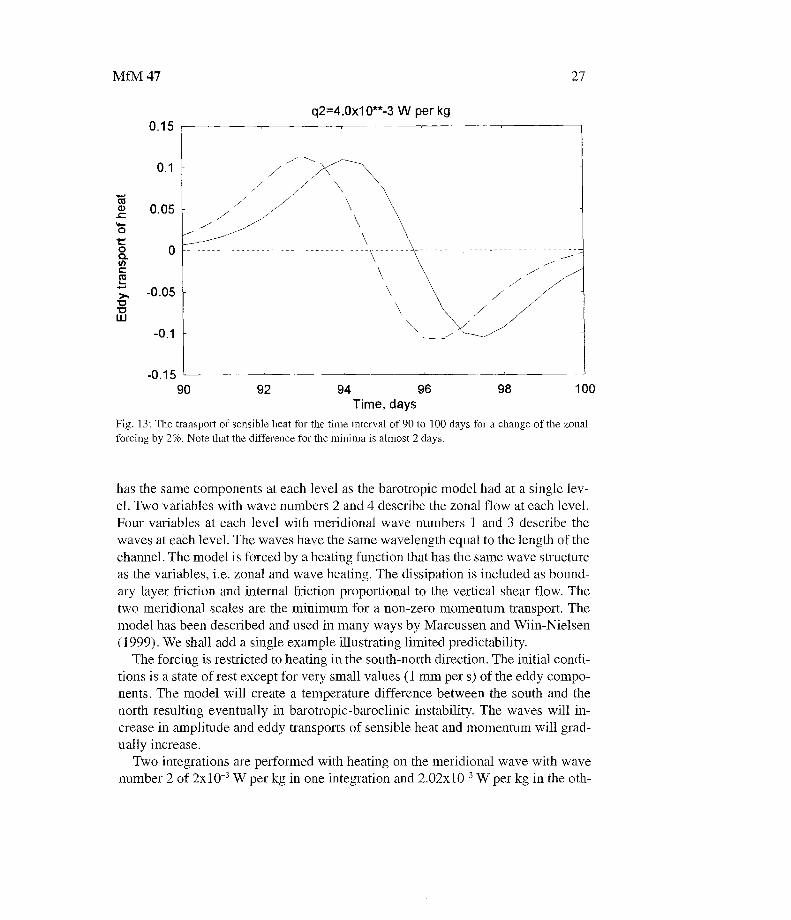
Figure 13 shows the maximum transport of sensible heat during the time interva lfrom 90 to 100 days . It is seen that a significant difference between the two inte-gration has taken place . This statement applies also to all the other dependent vari-ables .

Example F : Baroclinic model with heat- and momentum transpor tAs the final example of a meteorological nature we select still another low ordermodel containing 12 components, 6 at each of the two levels in the model, which

MfM 47

27

q2=4 .0x10""-3 W per kg0 .15

------------------ -- - --

- --

-

,,,,--

\

\

/

-0 .1590

92

94

96

98

100Time, days

Fig . 13 : The transport of sensible heat for the time interval of 90 to 100 days for a change of the zona lforcing by 2% . Note that the difference for the minima is almost 2 days .

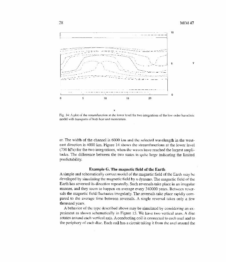
has the same components at each level as the barotropic model had at a single lev -el . Two variables with wave numbers 2 and 4 describe the zonal flow at each level .Four variables at each level with meridional wave numbers 1 and 3 describe th ewaves at each level . The waves have the same wavelength equal to the length of th echannel . The model is forced by a heating function that has the same wave structureas the variables, i .e . zonal and wave heating . The dissipation is included as bound-ary layer friction and internal friction proportional to the vertical shear flow. Thetwo meridional scales are the minimum for a non-zero momentum transport . Themodel has been described and used in many ways by Marcussen and Wiin-Nielse n(1999) . We shall add a single example illustrating limited predictability .

The forcing is restricted to heating in the south-north direction . The initial condi-tions is a state of rest except for very small values (1 inm per s) of the eddy compo-nents . The model will create a temperature difference between the south and thenorth resulting eventually in barotropic-baroclinic instability . The waves will in-crease in amplitude and eddy transports of sensible heat and momentum will grad-ually increase .

Two integrations are performed with heating on the meridional wave with wavenumber 2 of 2x10 -3 W per kg in one integration and 2 .02x10-3 W per kg in the oth -

0 . 1

-0 .1

28

MfM 47

5

Y

o

1 0

x

Fig . 14 : A plot of the streamfunction at the lower level for two integrations of the low order baroclini cmodel with transports of both heat and momentum.

er. The width of the channel is 6000 km and the selected wavelength in the west -east direction is 4000 km. Figure 14 shows the streamfunctions at the lower level(750 hPa) for the two integrations, when the waves have reached the largest ampli -tudes. The difference between the two states is quite large indicating the limite dpredictability.

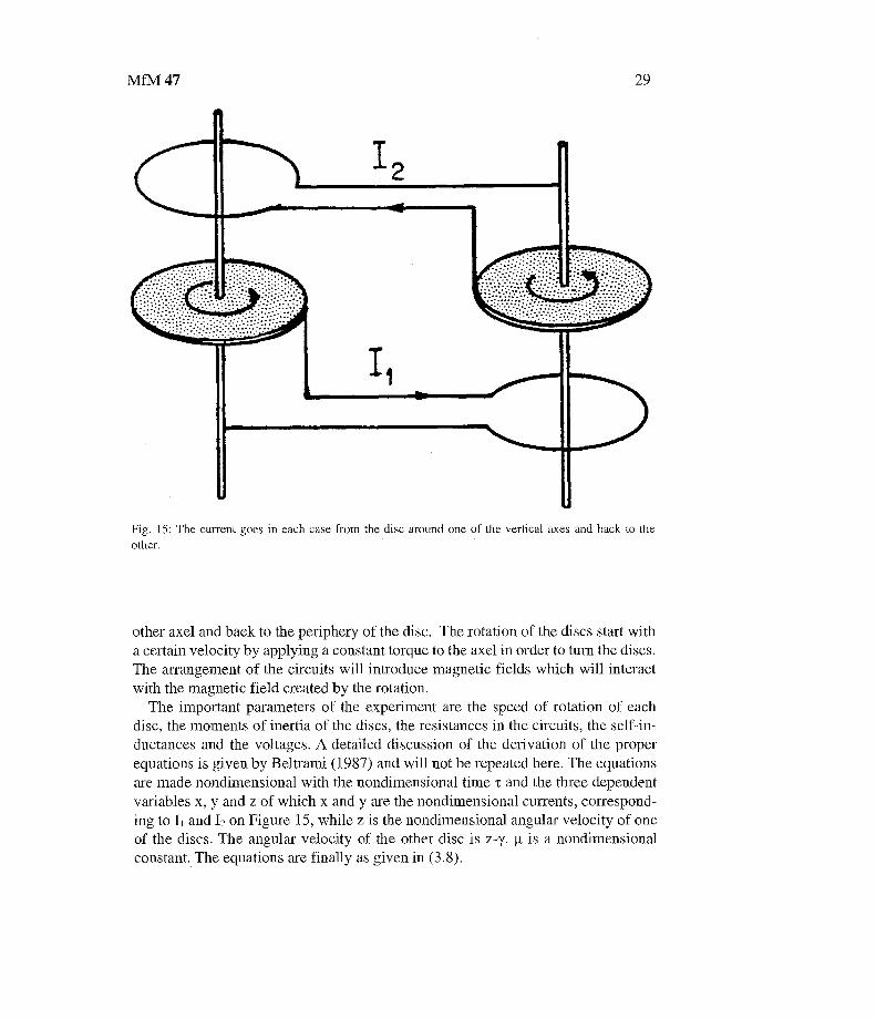
Example G. The magnetic field of the Eart hA simple and schematically correct model of the magnetic field of the Earth may b edeveloped by simulating the magnetic field by a dynamo . The magnetic field of th eEarth has reversed its direction repeatedly . Such reversals take place in an irregularmanner, and they seem to happen on average every 340000 years . Between rever-sals the magnetic field fluctuates irregularly . The reversals take place rapidly com-pared to the average time between reversals . A single reversal takes only a fe wthousand years .

A behavior of the type described above may be simulated by considering an ex-periment as shown schematically in Figure 15. We have two vertical axes . A discrotates around each vertical axis . A conducting coil is connected to each axel and t othe periphery of each disc . Each coil has a circuit taking it from the axel around the

MfM 47 29

Fig . 15 : The current goes in each case from the disc around one of the vertical axes and back to th eother .

other axel and back to the periphery of the disc . The rotation of the discs start witha certain velocity by applying a constant torque to the axel in order to turn the discs .The arrangement of the circuits will introduce magnetic fields which will interac twith the magnetic field created by the rotation .

The important parameters of the experiment are the speed of rotation of eac hdisc, the moments of inertia of the discs, the resistances in the circuits, the self-in-ductances and the voltages . A detailed discussion of the derivation of the properequations is given by Beltrami (1987) and will not be repeated here . The equationsare made nondimensional with the nondimensional time ti and the three dependen tvariables x, y and z of which x and y are the nondimensional currents, correspond -ing to I 1 and 12 on Figure 15, while z is the nondimensional angular velocity of oneof the discs . The angular velocity of the other disc is z-y . t is a nondimensionalconstant . The equations are finally as given in (3 .8) .

30

MfM 47

dx=

dz- Yz-/rx

dz= x(z-Y)-µY

dz

dz = 1-xy

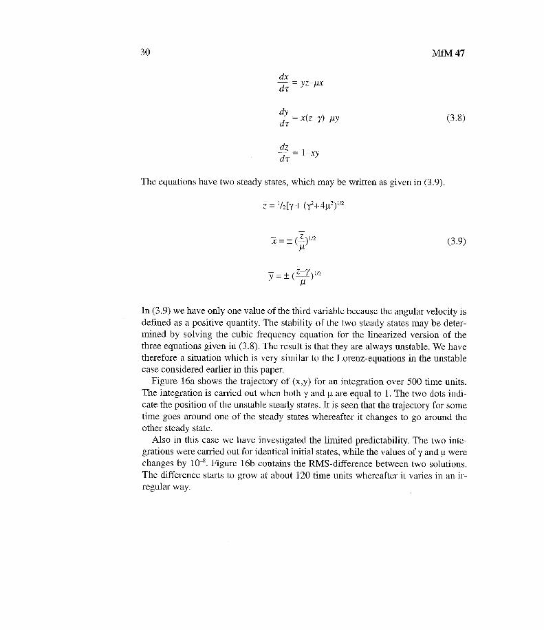
The equations have two steady states, which may be written as given in (3 .9) .

z = 'My + (y 2 +4µ2) 112

=+ O UZ

(3 .9 )

Ÿ= + (zY ) 1I2

P

In (3 .9) we have only one value of the third variable because the angular velocity i sdefined as a positive quantity. The stability of the two steady states may be deter -mined by solving the cubic frequency equation for the linearized version of th ethree equations given in (3 .8) . The result is that they are always unstable . We havetherefore a situation which is very similar to the Lorenz-equations in the unstabl ecase considered earlier in this paper .

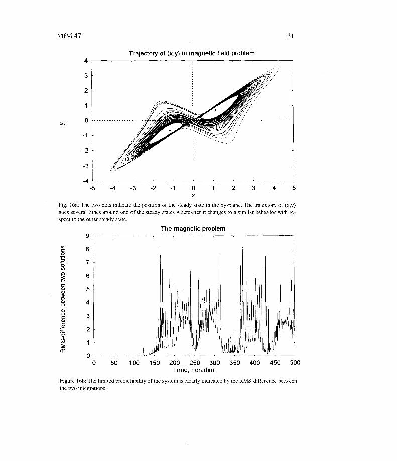
Figure 16a shows the trajectory of (x,y) for an integration over 500 time units .The integration is carried out when both y and µ are equal to 1 . The two dots indi-cate the position of the unstable steady states . It is seen that the trajectory for som etime goes around one of the steady states whereafter it changes to go around th eother steady state .

Also in this case we have investigated the limited predictability . The two inte -grations were carried out for identical initial states, while the values of y and µ werechanges by 10-8 . Figure 16b contains the RMS-difference between two solutions .The difference starts to grow at about 120 time units whereafter it varies in an ir -regular way.

(3 .8)

MfM 47

3 1

>,

Trajectory of (x,y) in magnetic field proble m

-5

-4

-3

-2

-1

1

2

3x

Fig . 16a: The two dots indicate the position of the steady state in the xy-plane . The trajectory of (x,y )goes several times around one of the steady states whereafter it changes to a similar behavior with re-spect to the other steady state .

The magnetic problem9

8

7

6

Ul

~~ h0

0

50

100 150 200 250 300 350 400 450 500Time, non .dim .

Figure 16b : The limited predictability of the system is clearly indicated by the RMS-difference betwee nthe two integrations .

4

3

- 1

-2

-3

-4

2

1

0

4

5

3

2

1

32

MfM 47

4. Limited predictability and the uncertainty of parameters

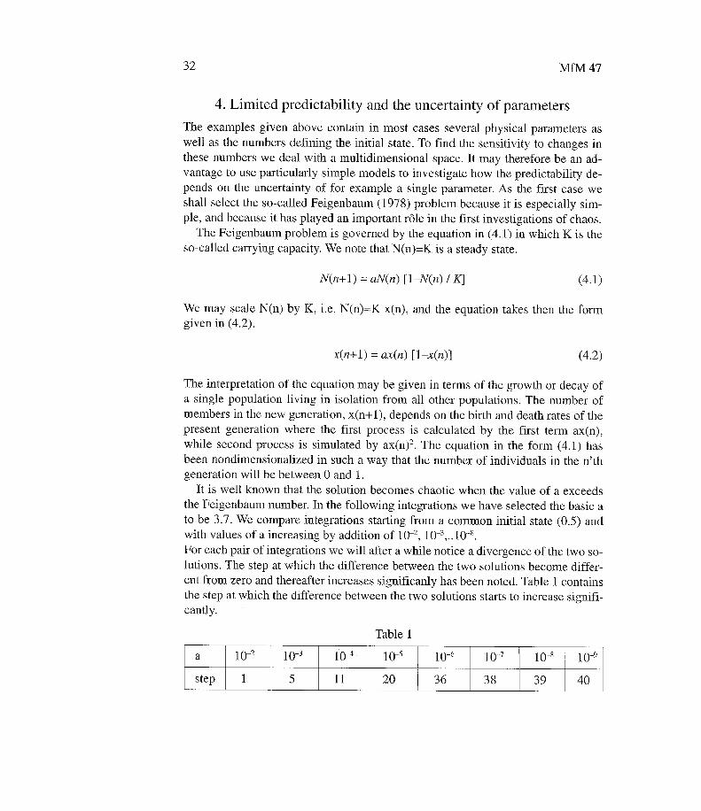
The examples given above contain in most cases several physical parameters a swell as the numbers defining the initial state . To find the sensitivity to changes i nthese numbers we deal with a multidimensional space . It may therefore be an ad -vantage to use particularly simple models to investigate how the predictability de -pends on the uncertainty of for example a single parameter . As the first case w eshall select the so-called Feigenbaum (1978) problem because it is especially sim-ple, and because it has played an important rôle in the first investigations of chaos .

The Feigenbaum problem is governed by the equation in (4 .1) in which K is theso-called carrying capacity . We note that N(n)=K is a steady state .

N(n+l) = aN(n) [1-N(n) / K]

(4 .1 )

We may scale N(n) by K, i .e . N(n)=K x(n), and the equation takes then the for mgiven in (4 .2) .

x(n+l) = ax(n) [1 -x(n)]

(4 .2 )

The interpretation of the equation may be given in terms of the growth or decay o fa single population living in isolation from all other populations . The number o fmembers in the new generation, x(n+l), depends on the birth and death rates of thepresent generation where the first process is calculated by the first term ax(n) ,while second process is simulated by ax(n) 2 . The equation in the form (4 .1) hasbeen nondimensionalized in such a way that the number of individuals in the n'thgeneration will be between 0 and 1 .

It is well known that the solution becomes chaotic when the value of a exceedsthe Feigenbaum number. In the following integrations we have selected the basic ato be 3 .7 . We compare integrations starting from a common initial state (0 .5) andwith values of a increasing by addition of 10-2, 10-3 , . .10- 5 .For each pair of integrations we will after a while notice a divergence of the two so -lutions . The step at which the difference between the two solutions become differ -ent from zero and thereafter increases significanly has been noted . Table 1 contain sthe step at which the difference between the two solutions starts to increase signifi -cantly.

Table 1

a 10-2 10-3 10' 10-5 10-5 l0-' 10- 5 10-9

step 1 5 11 20 36 38 39 40

MfM 47 3 3

For the basic value of a=3.7 we find that the predictability increases from the firs tstep to about step 40 .

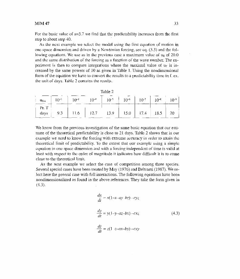
As the next example we select the model using the first equation of motion i none space dimension and driven by a Newtonian forcing, see eq . (3 .3) and the fol-lowing equations . We use as in the previous case a maximum value of UE of 20 . 0and the same distribution of the forcing as a function of the wave number . The ex-periment is then to compare integrations where the maximal value of uE is in-creased by the same powers of 10 as given in Table 1 . Using the nondimensionalform of the equation we have to convert the results to a predictability time in f . ex .the unit of days . Table 2 contains the results .

Table 2

uEm 10' 10- 3 10' 10 5 10 -5 10-7 10-8 10- 9

Pr. Tdays 9 .3 11 .6 12 .7 13 .9 15 .0 17 .4 18 .5 20

We know from the previous investigation of the same basic equation that our esti-mate of the theoretical predictability is close to 21 days. Table 2 shows that in ou rexample we need to know the forcing with extreme accuracy in order to attain thetheoretical limit of predictability. To the extent that our example using a simpl eequation in one space dimension and with a forcing independent of time is valid a tleast with respect to the order of magnitude it indicates how difficult it is to com eclose to the theoretical limit .

As the next example we select the case of competition among three species .Several special cases have been treated by May (1976) and Beltrami (1987) . We se -lect here the general case with full interactions . The following equations have beennondimensionalized as found in the above references . They take the form given i n(4 .3) .

dx =dt -

x(1-x-ay-bz) -cyz

~t = y(1y-az-bx) -cxz

dz=dt - z(l-z-ax-by) -cxy

(4 .3 )

34

MfM 47

These equations have a steady state where the three coordinates are equal to eac hother as given in (4 .4) .

_

1x-y_

_Z__

1+a+b+ c

No other steady states have been found . A stability analysis can be carried out in theusual wave by linearization around the steady state . The results of the stabilityanalysis gives three values of the frequencies . They are given in (4 .5) .

v,~lv 23=-(1-2c-1 lz(a+b)± ilai3vz (a-b) )

It is thus seen that the steady state will be stable if c satisfies the inequality given i n(4 .6) .

c<'l2(1-'l2(a +b))

(4 .6 )

The result in (4 .6) has been tested and verified by numerical integrations where th einitial values of x, y and z are equal . However, if an arbitrary initial state is used, itturns out that smaller values of c are needed, if the integration shall arrive in the sta -ble steady state .

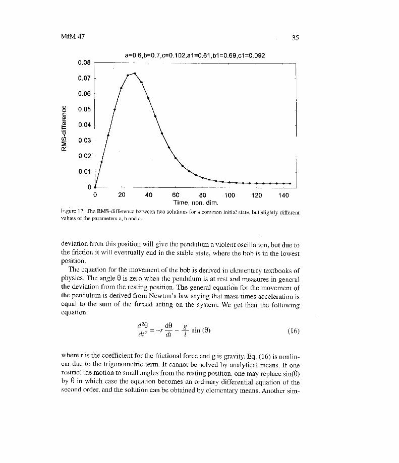
A single example will be shown . Two parallel integrations were performed wit ha common initial state (0 .9,0 .7,0 .3) . In one of the integrations a, b and c have th evalues 0.6, 0 .7 and 0.102, while the values 0 .61, 0 .69 and 0.092 were used in theother . Since the steady states are stable, the two integrations should reached thes esteady state asymptotically. Figure 17, showing the RMS-difference between thetwo integrations, shows that both of them arrive in the proper steady state .However, due to the difference in the values of the parameters the RMS values in -crease initially and reach rather large values after an integration time of about 3 0units . In this case of stable steady states we have only limited predictability in th eshort time range .

The pendulum is a classical example of a nonlinear system . We consider a pen-dulum consisting of a slim, rigid and massless rod of length 1 connected to a pivo tand ending in a bob of mass m. The pivot is made in such a way that the pendulu mcan move in a plane only . The forces working on the pendulum are gravity and thefriction from the air. Two steady states can be found . The first is the position wherethe bob is in the lowest position . This steady state is stable as we all know. The sec -ond stationary position is the case where the bob is in its highest position . A small

(4.4)

(4 .5)

MfM 47

35

a=0 . 6 , b=0 .7,c=0 .102,a1=0.61,b1=0.69,c1 =0 .0920 .08

0.07

0.06

0 .05

0 .04

0 .03

0 .02

0 .01

20

40

60

80

100

120

140Time, non . dim .

Figure 17 : The RMS-difference between two solutions for a common initial state, but slightly differen tvalues of the parameters a, b and c .

deviation from this position will give the pendulum a violent oscillation, but due tothe friction it will eventually end in the stable state, where the bob is in the lowestposition .

The equation for the movement of the bob is derived in elementary textbooks o fphysics . The angle 0 is zero when the pendulum is at rest and measures in generalthe deviation from the resting position . The general equation for the movement o fthe pendulum is derived from Newton's law saying that mass times acceleration i sequal to the sum of the forced acting on the system . We get then the followingequation :

zdt2 = -r

- g T sin (0)

(16)

where r is the coefficient for the frictional force and g is gravity. Eq . (16) is nonlin-ear due to the trigonometric term . It cannot be solved by analytical means. If onerestrict the motion to small angles from the resting position, one may replace sin(O )by 0 in which case the equation becomes an ordinary differential equation of th esecond order, and the solution can be obtained by elementary means . Another sim-

36

MfM 47

ple case is the one where it has been assumed that the frictional term may be ne-glected. In the general case the equation have to be treated by numerical integra-tion. It is an advantage to replace the single equation by two equations. We definex=9 and y=dO/dt. x may be named the position of the bob, while y is the angular ve -locity. We get then the following equations :

dxdt = y

dt = -ry -g sin (x)

We may be sure that the gravity g is known with excellent accuracy . The sam eshould be the case for length 1 of the rod . However, the coefficient representing thefriction included in the model is known with far less accuracy . The initial state i sgiven by the value xo , measuring the initial angle from the vertical position, wher ethe bob is in the lowest position, and the initial angular velocity y o , which in th e

Common init .st . :pi/4,0 ;r=0 .01,r1=0 .011

(17)

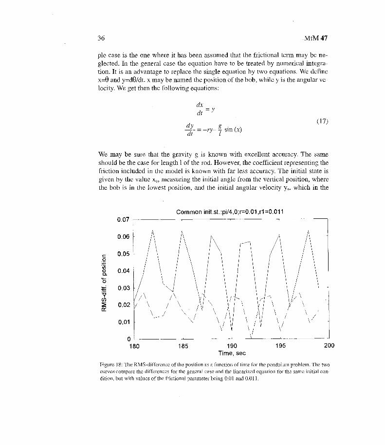
Figure 18 : The RMS-difference of the position as a function of time for the pendulum problem . The tw ocurves compare the differences for the general case and the linearized equation for the same initial con-dition, but with values of the frictional parameter being 0 .01 and 0 .011 .

MfM 47

37

x=pi/4,y=0 .0 ;x1 =pi/4+0 .01,y1 =0 .01 ;r= r1 =0.0 10 .03

0 .005

0 .025

0180

7 1

190

195

200Time, sec

18 5

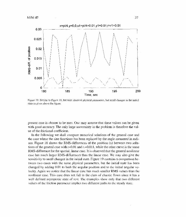
Figure 19 : Similar to Figure 18, but with identical physical parameters, but small changes in the initia lstate as given above the figure.

present case is chosen to be zero . One may assume that these values can be givenwith good accuracy . The only large uncertainty in the problem is therefore the val-ue of the frictional coefficient .

In the following we shall compare numerical solutions of the general case an dthe case where the sine functions has been replaced by the angle measured in radi -ans . Figure 18 shows the RMS-differences of the position (x) between two solu-tions of the general case with r=0 .01 and r,=0 .011, while the other curve is the sam eRMS-difference for the special, linear case . It is observed that the general nonlinea rcase has much larger RMS-differences than the linear case . We may also give th esensitivity to small changes in the initial state . Figure 19 contains a comparison be -tween two cases with the same physical parameters, but the initial state has bee nchanged by adding 0 .01 to both the angular position and to the initial angular ve-locity . Again we notice that the linear case has much smaller RMS-values than th enonlinear case. This case does not fall in the class of chaotic flows since it has awell defined asymptotic state of rest . The examples show only that two differen tvalues of the friction parameter implies two different paths to the steady state .

38

MfM 47

5 . Summary and concluding remarks

The purpose of the present paper is to discuss the limited predictability of nonlinearsystems. The weather predictions using atmospheric models have been selected i nSection 2 to illustrate limited predictability in a well documented geophysical fiel dwith experience covering half a century . Section 3 contains a number of low orderatmospheric models used to illustrate the main aspects of sensitivity to smal lchanges in the initial state or the forcing of the system . Section 3 contains also anattempt to estimate the theoretical limit of predictability .

During the last century we have gradually learned and tested that almost all non -linear systems show limited predictability . The nonlinear equations that can besolved in a closed mathematical form are very few and very simple . The originaloptimistic view that valid predictions could be made for unlimited times if the ini-tial state and the forcing were known with excellent accuracy has been replace dwith a much more realistic view, because we in most cases by numerical experi-ments can determine the operational limits of predictability, or, in other words, w ehave a better understanding of what we can and cannot do . At the same time it hasto be realized that this view have not so far been accepted by all groups engaged i npredictions of climate change and social and economical affairs .

Regarding the application of predictions it should be pointed out that prediction sfor a week or so do not permit any possibilities to influence the validity of the pre -dictions . The weather forecasts are valid for such a short time that anthropogeni cinfluences are negligible on this time scale . On the other hand, predictions of th esecond kind for extended periods such as predictions of climate change or predic-tions of an economic or social nature can indeed be counteracted by measures o ractivities that will influence the validity of the forecast . As a matter of fact, the pro-duction of economic forecasts is used by governments and institution to produc ecounter-measures that should decrease the impact of unwanted predicted develop-ments . Another example is the attempted simulations of the future climate change screated by anthropogenic influences on the climate . We shall as a matter of fac tnever have the possibility to verify the validity of these simulations when measure sare taken by governments and large institutions to decrease the anthropogenic in-fluences .

Other fields that have been investigated in some detail are competition amon gthree or more species (May and Leonard, 1975, May, 1976, Beltrami, 1987, Wiin-Nielsen, 1998) and population dynamics (Feigenbaum, 1978), but many other areasstill need to perfo,ui all the numerical experimentation necessary to determine th ebehavior of the prediction procedures in their field .

MfM 47

39

5 . Acknowledgement

The author would like to express his appreciation to Dr . D. Burridge, the Directorof the European Centre for Medium-Range Weather Forecasts, for providing infor -mation on operational predictability and its development over the last few years .

Appendix 1

The purpose of this appendix is to give an example of limited prediction in the clas-sical three body problem which gave the first example on limited predictability.The equations for the problem are well known and can be found in any book on the -oretical astronomy. We denote the masses of the three bodies by m, m, and ma, th eposition vectors by r, r, and r2 , the velocities by v, v, and v 2, and the distances be-tween the three bodies by ro ,, roe and r, 2 . The universal gravitational coefficient i sdenoted by µ . The vector equations of motion are then given in (Al) .

dv

ri-r

r2-r

dt

- turn 2rå r

rl-r

r2-r, +pm 2rôl

~ 2

dv2

r2-r

r2-r 1=pm +pm 2

The remaining three equations are simply the definition of the vector velocities asseen from (A2) .

dr

dt- = v

dr,- =dt -

v i

dr2

d t

dt

r o2

(Al )(Al )

(A2)

dt = v2

40

MfM 47

Initial values, z2=0 .05 and z2 =0.060 . 6

0 . 5

0 . 4

0 .1

0

-0 .1-0 .1

0

0 .1

0 .2

0.3

0 .4

0 . 5x1, non .dim .

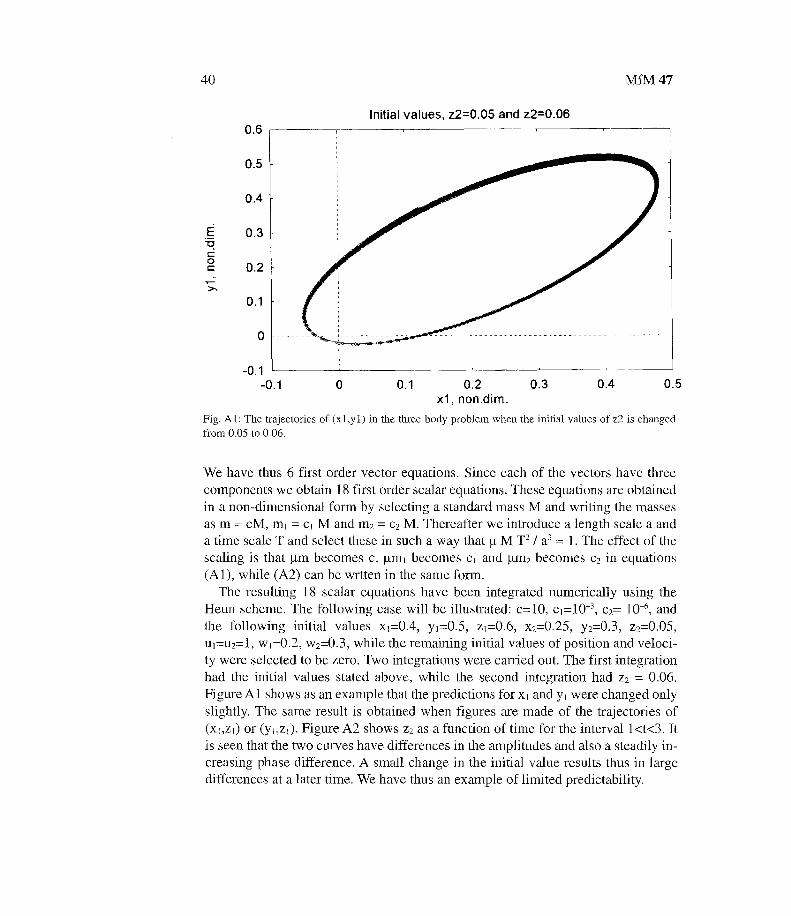
Fig. Al : The trajectories of (x I,yl) in the three-body problem when the initial values of z2 is change dfrom 0 .05 to 0 .06 .

We have thus 6 first order vector equations . Since each of the vectors have threecomponents we obtain 18 first order scalar equations . These equations are obtaine din a non-dimensional form by selecting a standard mass M and writing the massesas m = cM, m, = c, M and m 2 = e2 M. Thereafter we introduce a length scale a anda time scale T and select these in such a way that µ M T 2 / a3 = 1 . The effect of th escaling is that µm becomes c, µm, becomes c, and µm 2 becomes c2 in equations(Al), while (A2) can be wrtten in the same form .

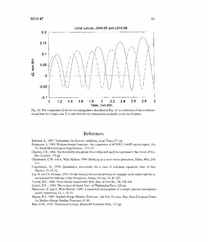
The resulting 18 scalar equations have been integrated numerically using th eHeun scheme . The following case will be illustrated : c=10, c,=10-3 , c2 = 10-x , andthe following initial values x,=0 .4, y,=0 .5, z,=0.6, x 2 =0.25, y 2 =0.3, z2=0.05 ,u,=u 2 =1, w,=0 .2, w 2 =0.3, while the remaining initial values of position and veloci-ty were selected to be zero . Two integrations were carried out . The first integrationhad the initial values stated above, while the second integration had z2 = 0.06 .Figure Al shows as an example that the predictions for x, and y, were changed onl yslightly. The same result is obtained when figures are made of the trajectories of(x,,z,) or (y,,z,) . Figure A2 shows z2 as a function of time for the interval 1<t<3 . Itis seen that the two curves have differences in the amplitudes and also a steadily in -creasing phase difference . A small change in the initial value results thus in larg edifferences at a later time . We have thus an example of limited predictability.

MfM 47 41

Initial values, z2=0 .05 and z2=0 .06

E

CO

NC

1

1 .2

1 .4

1 .6

1 .8

2

2 .2

2 .4

2 .6

2 .8

3Time, non .dim .

Fig . A2 : The component z2 for the two integrations described in Fig . Al as a function of the nondimen-sional time for 3 time units . It is seen that the two integrations gradually come out of phase .

Reference s

Beltrami, E., 1987 : Mathematic for dynamic modeling, Acad . Press, 277 pp .Bengtsson, L, 1985 : Medium-Range Forecasts - the experience at ECMWF, GARP special report,, No .

43, World Meteorological Organization,, 113-132 .Charney, J .G., 1966 : The feasability of a global observation and analysis experiment, Nat . Acad . of Sci . ,

Res . Council, 172 pp .Christensen, C .W. and A . Wiin-Nielsen, 1996 : Blocking as a wave-wave interaction, Tellus, 48A, 254 -

271 .Feigenbaum, M ., 1978: Quantitative universality for a class of nonlinear equations, Jour . of Stat.

Physics, 19, 25-52 .Lin, H . and J .F. Derome, 1995 : On the thermal interaction between the synoptic-scale eddies and the in-

tra-seasonal fluctuations in the atmosphere, Atmos .-Ocean ., 33, 81-107 .Lorenz, E.N ., 1963 : Deterministic nonperiodic flow, Jour . of Atm .Sci ., 20, 130-144 .Lorenz, E.N .,, 1993 : The essence of chaos, Univ . of Washington Press, 226 pp .Marcussen, P. and A . Wiin-Nielsen, 1999 : A numerical investigation of a simple spectral atmospheri c

model, Atm6sfera, 12, 1, 43-73 .Mason, B .J ., 1985 : Medium-Range Weather Forecasts - the first 10 years, Rep . from European Centre

for Medium-Range Weather Forecasts, 67-86 .May, R .M ., 1976: Theoretical Ecology, Blackwell Scientific Publ ., 317 pp .

42

MfM 47

May, R .M . and W.J . Leonard, 1975 : Nonlinear aspects of competition between three species, SIAM ,Jour. of Appl . Math ., 29, 243-252 .

Phillips, N.A., 1956 : The general circulation of the atmosphere : A numerical experiment, Quart . Jour.Roy. Met. Soc ., 82, 123 164 .

Platzman, G .W., 1960 : The spectral form of the vorticity equation, Jour . of Meteor ., 17, 635-644 .Plaut, G . and R . Vautard, 1994 : Spells of low-frequency oscillations and weather regimes in th e

Northern Hemisphere, Jour. Atm .Sci ., 51 210-236 .Poincaré, H ., 1893 : Les Méthodes nouvelle de la mechanique celeste, Paris, Gauthier-Villar .Poincaré, H ., 1912 : Science et Méthodes, Paris, Flammarion .Thompson, P.D ., 1957 : Uncertainty of initial state as a factor in predictability of large-scale atmospheri c

flow pattern, Tellus, 9, 275-295 .Wiin-Nielsen, A., 1961 : On short- and long-term variations in quasi-barotropic flow, Mo .Wea . Rev, 89 ,

461-476 .Wiin-Nielsen, A., 1991 : Comparison of low-order atmospheric systems, Atmôsfera, 5, 135-155 .Wiin-Nielsen, A ., 1992: Low-order baroclinic models forced by meridional and zonal heating ,

Geophysica, 27, 13-40 .Wiin-Nielsen, A., 1996 : A note on longer term oscillations in the atmosphere Atmôsfera, 9, 222-240 .Wiin-Nielsen, A ., 1997 : `Everybody talks about it . . .', Math.-Phys . Medd ., 44:1, Danish Royal Society

for Science and Humanities, 96 pp .Wiin-Nielsen A ., 1997 : On intermonthly oscillations in the atmosphere, Atmôsfera, 10, 23-42 .Wiin-Nielsen, A., 1998 : On the stable part of the Lorenz attractor, Atmôsfera, 11, 61-73 .Wiin-Nielsen, A., 1998 : Limited predictability (in danish), Kvant, 9, 21-25 .Wiin-Nielsen, A, 1999 : Steady states and transient solutions of the nonlinear forced shallow water equa-

tions in one space dimension, acc . for publ ., Atmôsfera, 12 .