PRECONDITIONING ORBITAL MINIMIZATION METHOD FOR …matyh/publications/sppOMM.pdf · A natural question is whether more ... The OMM method is highly efﬁcient in each iteration,

PRECONDITIONING ORBITAL MINIMIZATION METHOD FOR PLANEWAVE

DISCRETIZATION

JIANFENG LU AND HAIZHAO YANG

ABSTRACT. We present an efficient preconditioner for the orbital minimization method when the

Hamiltonian is discretized using planewaves (i.e., pseudospectral method). This novel precondi-

tioner is based on an approximate Fermi operator projection by pole expansion, combined with

the sparsifying preconditioner to efficiently evaluate the pole expansion for a wide range of Hamil-

tonian operators. Numerical results validate the performance of the new preconditioner for the

orbital minimization method, in particular, the iteration number is reduced to O (1) and often only

a few iterations are enough for convergence.

1. INTRODUCTION

We consider the problem of finding the low-lying eigenspace of a Hamiltonian matrix H com-

ing from the planewave discretization of a self-adjoint Hamiltonian operator − 12∆+V for some

potential function V . Given an n×n Hamiltonian matrix H , it is well-known that, the eigenspace

associated to the first N eigenvalues (non-degeneracy is assumed throughout the work) is given

by the trace minimization

(1) E = minX∈Cn×N , X ∗X=IN

tr(X ∗H X ),

where IN is a N × N identity matrix, thus X ∗X = IN is the orthonormality constraints of the

columns of X . When a conventional algorithm is used to solve for the eigenvalue problem, a

QR factorization in each iteration is required to impose orthogonality. The computational cost

of each QR is O (nN 2) with a large prefactor and communication cost is expensive in high per-

formance computing. This creates an obstacle to minimize (1) if the number of iteration is large.

Much effort has been devoted to reducing the communication cost, see e.g., [5,18] and references

therein.

It turns out that it is in fact possible to remove the orthogonality constraint. In the context of

linear scaling algorithms for electronic structure calculations, the orbital minimization method

(OMM) was proposed in [19–22] to circumvent the orthonormality constraint in (1). Instead, we

search for the eigenspace by an unconstrained minimization

(2) E = minX∈Cn×N

Eomm(X ) = minX∈Cn×N

tr((2IN −X ∗X )(X ∗H X )

).

Date: March 31, 2016.Key words and phrases. Kohn-Sham density functional theory, orbital minimization method, preconditioning, Fermi

operator projection, pole expansion, sparsifying preconditioner.This work is partially supported by the National Science Foundation under grants DMS-1312659, DMS-1454939, and

ACI-1450280. H.Y. thanks the support of the AMS-Simons Travel Award. We thank Lexing Ying for helpful discussions.

1

2 JIANFENG LU AND HAIZHAO YANG

To see where (2) comes from, notice that we may reformulate (1) to relax the orthogonality con-

straint as

(3) E = minX∈Cn×N , rank X=N

tr((X ∗X )−1(X ∗H X )

),

so that X is no longer constrained. The factor (2IN −X ∗X ) in (2) can then be seen as a Neumann

series expansion of (X ∗X )−1 = (IN − (IN −X ∗X )

)−1 truncated to the second term.

Somewhat surprisingly, for negative definite H (all the eigenvalues are strictly less than 0), the

minimizer of Eomm spans the same subspace as the minimizer to the original problem (1), thus

the desired eigenspace [19, 20]. Note that the assumption that H being negative definite can be

made without loss of generality, as we may just shift the diagonal of H by a constant, and this

shift will not change the eigenspace.

The OMM was originally proposed for linear scaling calculations (the total computational cost

is linearly proportional to N , the number of electrons) for sparse H , combined with truncat-

ing X to keep only O (1) entries per column. However, even without adopting the linear scaling

truncation, whose error can be hard to control, in the context of cubic scaling implementation,

the OMM algorithm still has advantage over direct eigensolver in terms of scalability in parallel

implementations [3]. The OMM has the potential to be a competitive strategy for finding the

eigenspace.

Since the OMM transforms the eigenvalue problem into an unconstrained minimization, the

nonlinear conjugated gradient method is usually employed to minimize the energy (2). The effi-

ciency of the OMM algorithm thus depends on the optimization scheme, which in turn crucially

depends on the preconditioner.

In this work, we will consider H coming from a Fourier pseudospectral discretization of the

Hamiltonian operator. The pseudospectral method typically requires minimal degree of free-

doms for a given accuracy among standard discretizations and is also easy to implement using

the fast Fourier transform (FFT), and hence widely used in the field physics and engineering liter-

ature. In the field of electronic structure calculation, it is known as the planewave discretization,

which is arguably the most popular discretization scheme up-to-date.

While the importance of preconditioning for planewave discretization is well known and has

been long recognized [30]; the preconditioner has been mostly limited to the type of shifted in-

verse Laplacian (more details later). A natural question is whether more efficient preconditioner

can be designed.

We revisit the issue of preconditioning for planewave discretization. We propose a new pre-

conditioner using an approximate Fermi operator projection based on the pole expansion (see

e.g., [1, 7, 8, 15, 26]). Once constructed, the new preconditioner can be applied efficiently and

reduces the number of iteration of the OMM to only a few. The resolvents involved in the pole

expansion are solved iteratively using GMRES [29] combined with the recently developed sparsi-

fying preconditioner [17, 31, 32]. Since only an approximate Fermi operator is required, the con-

struction and application of preconditioner become quite efficient. Hence, the overall precondi-

tioned OMM requires much less computational time compared to existing OMM algorithms for

planewave discretizations.

This paper is organized as follows. In Section 2, existing preconditioned OMMs are introduced

and analyzed to motivate the design of the new preconditioner. In Section 3, we construct the

PRECONDITIONING ORBITAL MINIMIZATION METHOD FOR PLANEWAVE DISCRETIZATION 3

new preconditioner base on the approximate Fermi operator projection and the sparsifying pre-

conditioner. In Section 4, some numerical examples are provided to demonstrate the efficiency

of the new preconditioner. We conclude with a discussion and some future work in Section 5.

2. PRECONDITIONED ORBITAL MINIMIZATION METHOD

2.1. Orbital minimization method. The orbital minimization method (OMM) has become a

popular tool in electronic structure calculations for solving the Kohn-Sham eigenvalue problem.

One of the major advantage is that unlike conventional methods for eigenvalue calculations, no

orthogonalization is required in the iteration. The OMM minimizes the functional Eomm, recalled

here:

E = minX∈Cn×N

Eomm(X ) = minX∈Cn×N

tr((2IN −X ∗X )(X ∗H X )

).

The nonlinear conjugate gradient method is usually applied for this unconstrained minimiza-

tion problem. When the minimization problem becomes ill-conditioned (for example, when the

spectral gap, the difference between the N -th and (N + 1)-th eigenvalues, is small; further dis-

cussed below), it requires a large number of iterations to achieve convergence. Hence, an effi-

cient preconditioner is crucial to this minimization problem.

Let us consider preconditioning the gradient of Eomm in the general framework of nonlinear

conjugate gradient methods. Denote the gradient as

(4) G (X ) := δEomm(X )

δX ∗ = 2H X −X (X ∗H X )−H X (X ∗X ).

The preconditioned nonlinear conjugate gradient method can be summarized as follows.

1 Initialize: Pick initial guess X1 and fix a preconditioner P ;

2 Set D1 =−P G (X1) and perform a line search in the direction of D1 and update X2;

3 Set m = 2;

4 while not converged do5 Calculate the preconditioned gradient direction: Gm =−P G (Xm);

6 Compute βm according to the Polak-Ribière formula (other choices are equally possible)

βm = G∗m(Gm −Gm−1)

G∗m−1Gm−1

;

7 Update the conjugate direction Dm =Gm +βmGm−1;

8 Perform a line search in the direction of Dm and update Xm+1;

9 Set m = m +1.

Algorithm 1: Preconditioned nonlinear conjugate gradient method.The OMM method is highly efficient in each iteration, as involves only matrix-matrix multipli-

cations that take O (nN 2+N n logn) operations, where n logn comes from the FFT in the applica-

tion of H (recall that a pseudospectral discretization is used). Hence, a good preconditioner for

the OMM should be efficient to construct and simple to apply, so that it does not increase much

the cost of each iteration; at the same time, we hope the preconditioner can reduce the number

of iterations significantly.


2.2. Existing preconditioners. We shall first recall existing preconditioners for planewave dis-

cretization in general, which also apply for the OMM. The conventional preconditioning em-

ployed in the electronic structure calculation is in a form of inverse shifted Laplacian:

P = P ⊗ IN , where, P = (I −τ−1∆)−1.

Here −∆ stands for the discretization of the Laplacian operator (kinetic energy operator in the

Hamiltonian), and τ is a parameter setting the scale for the kinetic energy preconditioning. Note

that in the planewave discretization, P is a diagonal matrix in the k-space

(5) Pkk ′ = δkk ′ (1+τ−1|k|2)−1,

and thus application of the preconditioner has minimal computational cost.

In practice, the preconditioner might take a more complicated expression (see e.g., the review

article [23] and references therein)

(6) Pkk ′ = δkk ′27+18s +12s2 +8s3

27+18s +12s2 +8s3 +16s4

with s = |k|2/τ and τ a scaling parameter. This preconditioner was first proposed in [30] and is

now known as the TPA preconditioner. It has a similar asymptotic behavior to (5) around |k| = 0

and as |k|→∞, but is found to be more efficient than (5) empirically.

A recent article [33] generalized the TPA preconditioner using polynomials with higher degrees

than those in (6). More specifically, this new preconditioner, denoted as the generalized TPA

preconditioner (gTPA), is based on a polynomial of degree t

pt (s) := c0 + c1s + c2s2 +·· ·+ct s t ,

and takes the form

(7) Pkk ′ = δkk ′pt (s)

pt (s)+ ct+1s t+1 ,

where s = |k|2/τ as before. The polynomial pt is constructed such that all the derivatives of

g t (s) = pt (s)pt (s)+ct+1st+1 up to order t at s = 0 vanish, meaning that the gTPA preconditioner is close to

an identify operator in the low frequency regime and the width of this region depends on t . Note

that, the TPA preconditioner is a special case of the gTPA preconditioners for t = 3 and the shifted

Laplacian preconditioner in (5) is a special case of t = 0. From now on, Pt is used to denote the

gTPA preconditioner corresponding to t . In the pseudospectral method, applying all the precon-

ditioners above to a search direction only takes O (N n logn) operations since FFT is applied to N

columns in the search direction G (Xm).

The physical intuition of all these preconditioners is that: 1) the preconditioner should keep

the low-frequency components in the search direction unchanged; 2) g t should have an asymp-

totic behavior like 1s so that it behaves as an inverse Laplacian for the high-frequency compo-

nents. Therefore, they act as a low-pass filter that is essentially similar to the inverse shifted

Laplacian in 5. For the gTPA, as t increases, the low-frequency region is expanded while the high

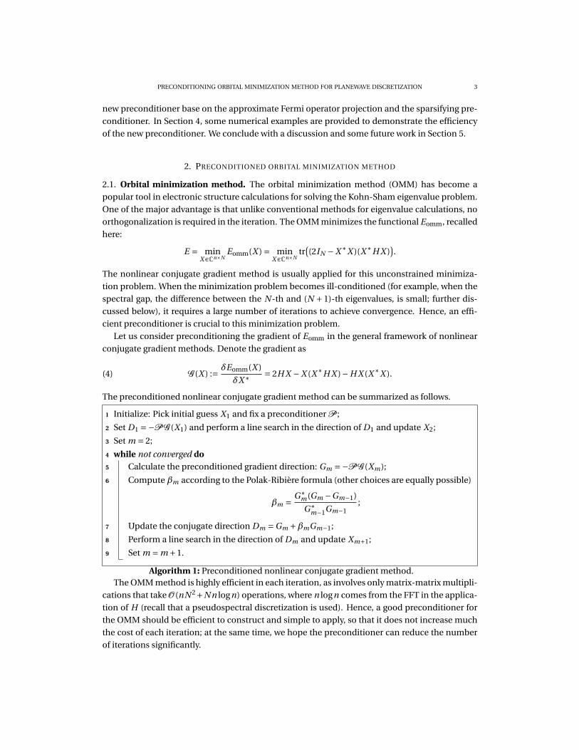
frequency components are further damped (see Figure 1 for an illustration).

As the behavior of these preconditioners is close to inverse shifted Laplacian, the success

essentially lies in the assumption that the potential part of the Hamiltonian operator does not

change the spectrum too much. When this assumption is not valid, these preconditioner might

not be able to effectively reduce the condition number of the OMM.


0 2 4 6 80

0.1

0.2

0.3

0.4

0.5

0.6

0.7

0.8

0.9

1

s

gt(s

)

t=1

t=3

t=5

FIGURE 1. The function g t (x) in the gTPA preconditioner for t = 1, 3, and 5.

2.3. Condition number of the preconditioned OMM. To understand the performance of the

existing preconditioners in the context of OMM, we analyze here the condition number of the

preconditioned OMM. While the condition number of the OMM (without preconditioning) was

analyzed in [24], for completeness, we will also repeat the calculation here in a slightly different

and more compact way.

Note that condition number of the TPA type preconditioning is rather complicated (if possi-

ble) to obtain analytically. For the purpose of simplicity, we consider a preconditioner of the type

of inverse shifted Hamiltonian

(8) P = (H −µI )−1,

which is more friendly for analysis (since it commutes with the Hamiltonian operator) and shares

the same spirit with the TPA type preconditioners. In fact, as it takes into account both the kinetic

and potential parts of the Hamiltonian, it captures better the spectral behavior of the Hamilton-

ian operator.

The Hessian of Eomm is given by

(9) H (X )Z = 2H Z −Z (X ∗H X )−X (Z∗H X )−X (X ∗H Z )−H Z (X ∗X )−H X (Z∗X )−H X (X ∗Z ).

Let X0 be the minimizer (i.e., the solution of the eigenvalue problem) such that H X0 = X0Λ0,

where Λ0 is a diagonal matrix containing the eigenvalues. Evaluating the Hessian at the mini-

mizer X0 (orthonormalized such that X ∗0 X0 = IN ), we have

(10) H (X0)Z = H Z −ZΛ0 −X0Z∗X0Λ0 −X0Λ0Z∗X0 −2X0Λ0X ∗0 Z .

Note that the energy Eomm is invariant under any perturbation in the subspace of X0, we may

assume that the perturbed direction is perpendicular, i.e., Z∗X0 = 0. For such directions, we get

(11) H (X0)Z = H Z −ZΛ0.


Therefore, the condition number of H is at least

(12) cond(H (X0)) ≥ λn −λ1

λN+1 −λN,

determined by the ratio of the spectrum width of H and the spectral gap. In particular, this im-

plies that if the gap between λN and λN+1 is small relatively to the whole spectrum width of H ,

the condition number of the OMM minimization becomes large.

For the preconditioned gradient, we get

(13) P G (X ) = 2PH X −P X (X ∗H X )−PH X (X ∗X ),

and thus

(14) P H (X0)Z = PH Z −P ZΛ0.

The eigenvalues of the Hessian hence depend on P (H −λi I ), i = 1, . . . , N , and some of them take

the form

(15) 1− λi −µλ j −µ

, i ≤ N < j .

To guarantee that the Hessian after preconditioning is positive definite, we consider the family

of preconditioner with P = (H −µI )−1 with µ < λN+1. To estimate the condition number after

preconditioning, we separate into several cases according to the position of µ in the spectrum of

H .

• λN < µ < λN+1, then the largest and the smallest eigenvalues of the form (15) after pre-

conditioning are

λmax = 1− λ1 −µλN+1 −µ

,

λmin = 1− λN −µλn −µ ,

since i ≤ N and N +1 ≤ j . Then the condition number is at least

(16) cond(P H (X0)) ≥1− λ1−µ

λN+1−µ1− λN−µ

λn−µ= λN+1 −λ1

λn −λN

λn −µλN+1 −µ

.

To minimize the condition number, we let µ→λN and get

(17) cond(P H (X0)) ≥ λN+1 −λ1

λN+1 −λN.

• λ1 <µ<λN , then

λmax = 1− λ1 −µλN+1 −µ

,

λmin = 1− λN −µλN+1 −µ

,

since i ≤ N and N +1 ≤ j . Then the condition number is at least

(18) cond(P H (X0)) ≥1− λ1−µ

λN+1−µ1− λN−µ

λN+1−µ= λN+1 −λ1

λN+1 −λN.


• µ≤λ1, then

(19) cond(P H (X0)) ≥1− λ1−µ

λn−µ1− λN−µ

λN+1−µ= λn −λ1

λN+1 −λN

λN+1 −µλn −µ .

To minimize the condition number, we should take µ close to λ1 in this case, which leads

to

(20) cond(P H (X0)) ≥ λN+1 −λ1

λN+1 −λN.

Therefore, we arrive at the conclusion that the lower bound of the conditioner we can achieve

by using a preconditioner of type P = (H −µI )−1 with µ<λN+1 is

λN+1 −λ1

λN+1 −λN.

Hence, the condition number after preconditioning will still be large if the spectral gap between

λN and λN+1 is small.

The above conclusion can be understood by investigating the spectral meaning of an inverse

shifted Hamiltonian of the form (H −µI )−1, we see that this type of preconditioners prefers the

eigenspace with eigenvalues close to the shift µ. This would limit the search direction in this

spectral window and hence the OMM cannot converge to the right solution quickly, or even con-

verges to an undisired solution. This motivates us to propose a new preconditioner based on

an approximate Fermi operator projection that restricts the search direction in the full target

eigenspace. This algorithm is presented in the next section.

3. ALGORITHM DESCRIPTION

The preconditioner we propose is based on the idea of using an approximate Fermi operator

projection, as described in Section 3.1. The preconditioner has the form of a linear combination

of shifted inverses of the Hamiltonian; so that to accelerate the construction and application, the

sparsifying preconditioner [31] is used to iteratively solve the linear equation corresponds to the

shifted inverse. The detail is given in Section 3.2. Last, it is possible to precompute and store

the preconditioner in a data sparse format using rank revealing QR decomposition, as will be

discussed in Section 3.3.

3.1. Fermi operator projection. In quantum mechanics, given an effective one-particle Hamil-

tonian H , the zero-temperature single-particle density matrix Π of the system is given by the

Fermi operator via a Green’s function expansion

(21) Π= 1

2πi

∫Γ

(zI −H)−1d z,

where Γ is a contour in the complex plane containing the N eigenvalues below the Fermi level.

Note that by Cauchy’s integral formula,Πdefined in (21) is exactly the projection to the eigenspace

corresponds to the first N eigenvalues. The contour integral representation of the Fermi operator

has been a useful tool in electronic structure calculation, for example in linear scaling methods

(see e.g., the review [8]). More recently, the contour integral formulation was used in the method

of PEXSI [14–16] for a fast algorithm to obtain the density for sparse Hamiltonian matrices, com-

bined with the selected inversion algorithm. It is also used in FEAST [26] as a general eigenvalue


solver for sparse Hamiltonian matrices. In [4], the contour integral was used for multishift prob-

lems. Our idea in this work is to explore the approximate Fermi operator projection as an effective

preconditioner.

To use Π as an preconditioner, similar to what we did in [15], we employ the efficient quadra-

ture rule proposed in [9] to discretize the contour integration (21) as

(22) Π≈p∑

j=0w j (H − z j I )−1

where z j is the j -th quadrature node on the contour and w j is its corresponding weight. The

above formula is also called pole expansion, as the quadrature points can be viewed as poles in

the resolvents (H − z j I )−1 in the expansion. The approximation error of the quadrature rule is

bounded by [15]

e−cp

(log

λn−λ1λN+1−λN

+3)−1

.

The convergence of the quadrature rule is exponentially fast in p and hence only a small number

of poles are needed. The details of the choice of w j and z j can be found in [15] and we will not

repeat here.

We remark that if the projection is calculated by inverting (H − z j I )−1 exactly (or with a very

small error tolerance), we get already the projection Π onto the low-lying eigenspace, i.e., the

density matrix. Of course, direct inversion of (H − z j I )−1, for pseudospectral discretization, is

equally expensive, since H is a dense matrix. This is different from the situation of PEXSI or

FEAST where sparse Hamiltonian matrices are considered. An alternative approach to construct

a precise projection is to use iterative matrix solvers to apply (H−z j I )−1. If a basis of the eigenspace

is desired, it can be obtained by acting Π on a few vectors, as in the Fermi operator projection

method [1, 8], or more systematically, by using a low-rank factorization via a randomized SVD

[10]. However, to obtain high accuracy, this idea is still expensive since the matrix (H − z j I ) is

usually ill-conditioned and the iteration number might be large.

The key observation is that, as we plan to apply the projection as a preconditioner, we in fact

do not really need the exact projection, as long as we can get a good approximation. Thus, it

suffices to use an iterative scheme to solve (H−z j )−1 acting on some vector with a relatively large

error tolerance. We aim to achieve a balance, such that the approximate projection is accurate

enough such that the OMM converges in a few iterations, but also rough enough such that the

construction is cheap.

More specifically, in the nonlinear conjugate gradient method for the OMM, the precondi-

tioned gradient direction at the m-th step is computed by

(23) Gm =−P G (Xm) =−p∑

j=0w j Ym, j ,

where Ym, j ∈Rn×N is a rough solution of the linear system

(24) (H − z j I )Ym, j =G (Xm),

for j = 1, . . . , p. In the pseudospectral method, the matrix H − z j I can be applied efficiently

via the FFT in O (n logn) operations. Hence, the GMRES [29] with a large tolerance and a small

number of maximum iterations is able to provide rough solutions to the linear systems in (24)

quickly. Denote the number of iterations in GMRES by ng , the total complexity for finding a


rough solution is O (png N n logn), which is of the same order as the complexity of the regular

TPA and gTPA preconditioners. To further accelerate the GMRES iteration, the search direction

G (Xm) is used as the initial guess for the GMRES, since it is almost in the eigenspace of interest if

m is large. As we shall see later, the new preconditioner is highly efficient and the preconditioned

OMM will converge in only a few iterations.

3.2. Sparsifying preconditioner. In the previous subsection, an approximate Fermi operator

projection is introduced as a preconditioner for the OMM. As we shall see later in the numeri-

cal section, the preconditioned OMM converges quickly in a few iterations. Hence, the difficulty

of solving an eigenvalue problem with the OMM has been replaced by the difficulty of construct-

ing the projection efficiently, the most expensive part of which is solving linear systems with

multiple right-hand sides. Since these linear systems are solved roughly in an iterative scheme

like the GMRES, the preconditioning problem for the OMM is transferred to the preconditioning

problem for the GMRES.

In the case when the Hamiltonian operator H = − 12∆+V −µ behaves like a kinetic energy

operator, i.e., the potential energy operator is negligible, a conventional preconditioner for the

linear system

(25) (H −µI )u = b

is

P = (−1

2∆− s)−1,

where s is a proper shift. However, when the contribution of the potential energy operator V is

large, e.g., in highly indefinite systems on periodic structures, an inverse shifted Laplacian is no

longer an efficient preconditioner, e.g., the GMRES might take a very large number of iterations

to converge or it even diverges. To overcome this difficulty, we will adopt the recently proposed

sparsifying preconditioner for solving the linear systems in the construction of the approximate

Fermi operator projection.

Let us focus on the numerical solution of (25). We assume that the computation domain is the

periodic unit box [0,1]d and discretize the problem using the Fourier pseudospectral method.

With abuse of notations, the discretized problem of (25) takes the form

(26)(−1

2∆+V −µ)

u = b.

We will briefly recall the key idea of the sparsifying preconditioner for solving this type of equa-

tions. More details can be found in [31] (see also [17, 32]).

Denote l = ⟨V ⟩ the spatial average of V . We assume without loss of generality that − 12∆+ l −µ

is invertible onTd with periodic boundary condition, otherwise, we will use a slight perturbation

of µ instead and put the difference into V . This allows us to rewrite (25) trivially as

(27)(−1

2∆+ (l −µ)+ (V − l )

)u = b

Applying the Green’s function of the constant part G = (− 12∆+ (l −µ)

)−1 via the FFT to both sides

of (25), we have an equivalent linear system

(28)(I +G(V − l )

)u =Gb.


The main idea of the sparsifying preconditioner is to multiply a particular sparse matrix Q (to

be defined later) on the both hand sides of (28):

(29) (Q +QG(V − l ))u =Q(Gb),

so to make the matrix on the left hand in (29) becomes sparse. To see how this is possible, let

S = {( j , a( j )), j ∈ J } be the support of the sparse matrix Q, i.e., for each point j , the row Q( j , :) is

supported in a local neighborhood a( j ). If for each point j , the Q is constructed such that

(QG)( j , a( j )c ) =Q( j , a( j ))G(a( j ), a( j )c ) ≈ 0,

then the product QG is also essentially supported on S. The sum Q +QG(V − l ) is essentially

supported in S as well, since (V − l ) is a diagonal matrix. The above requirement can indeed

be achieved since G , after all, is the Green’s function of a local operator; thus Q is a discrete

approximation of the differential operator. More details can be found in [31].

Restricting Q +QG(V − l ) to S by thresholding other values to zero, we define a sparse matrix

P

(30) Pi j ={(

Q +QG(V − l ))

i j , (i , j ) ∈ S,

0, (i , j ) 6∈ S.

Since P ≈Q +QG(V − l ), we have the approximate equation

(31) Pu ≈Q(Gb).

The sparsifying preconditioner computes an approximate solution u by solving

Pu =Q(Gb).

Since P is sparse, the above equation can be solved by sparse direct solvers such as the nested dis-

section algorithm [6]. The solution u = P−1QGb can be used as a preconditioner for the standard

iterative algorithms such as GMRES [29] for the solution of (26).

In the construction of the sparsifying preconditioner, the most expensive part is to build the

nested dissection factorization for P , the complexity of which scales as O (n1.5) in two dimensions

and O (n2) in three dimensions. The application of the sparsifying preconditioner is very efficient

and takes only O (n logn) operations in two dimensions and O (n4/3) operations in three dimen-

sions. Since the dominant cost of the OMM with pseudospectral discretization is O (nN 2), where

N is proportional to n, the construction and the application of the sparsifying preconditioner is

relatively cheap for large-scale problems. As we shall see in the numerical section, even if n is as

small as 576, the preconditioned OMM with the sparsifying preconditioner is still more efficient

than the one with a regular preconditioner.

3.3. Precomputing the preconditioner. When the problem size n is not sufficiently large, the

prefactor png in the application complexity of the approximate projection might be too large. It

is better to use a randomized low-rank factorization method to construct a matrix representation

UU∗ of the preconditioner such that

UU∗b ≈p∑

j=0w j (H − z j I )−1b,


for an arbitrary vector b ∈ Rn , where U ∈ Cn×N is a unitary matrix (and hence the notation U ).

Therefore, UU∗ is a data-sparse way to store the matrix preconditioner. Adapting the random-

ized SVD method [10], a fast algorithm for constructing the matrix U is given below.

1 Given the Hamiltonian H and the range of the eigenvalues, construct the quadrature nodes

and weights {z j , w ; j }1≤ j≤p for the contour integration in 21;

2 Construct a Gaussian random matrix B ∈Rn×N+k , where k is a non-negative constant

integer;

3 Solve the linear systems (H − z j I )Y j = B for each j = 1, . . . , p using the GMRES with the

right-hand side as the initial guess.

4 Compute Y =∑pj=0 w j Y j ;

5 Apply a rank-revealing QR factorization [U ,R] = qr(Y );

6 Update U by selecting the first N columns: U =U (:,1 : N );

7 The approximate Fermi operator projection is given by UU∗.

Algorithm 2: Randomized low-rank factorization for the Fermi operator projection.

The operation complexity of Algorithm 2 is O (png N n logn+nN 2), where nN 2 comes from the

QR factorization. When N is very large and nN 2 dominates the construction complexity of the

preconditioner, it is better to apply the projection in (23) directly without the QR factorization,

while for smaller scale problems, the pre-computation accelerates the overall calculation.

We remark that the scalability of the rank-revealing QR factorization in high performance

computing has been an active research direction, see for example the communication-reduced

QR factorization recently proposed in [18] and implemented in Elemental [28]. Due to the large

prefactor of the complexity of the communication-reduced QR factorization, applying it for many

times is still quite expensive. This makes Algorithm 2 better than those with QR factorization in

each iteration, e.g., in conventional ways to solve for 1. Parallelism of other steps is straightfor-

ward: 1) each linear system at each pole z j can be solved simultaneously; 2) parallel GMRES rou-

tines have been standard in high performance computing; 3) applying this approximate Fermi

operator projection is simple matrix-matrix multiplication with complexity O (nN 2).

4. NUMERICAL EXAMPLES

This section presents numerical results to support the efficiency of the proposed algorithm.

Numerical results were obtain in MATLAB on a Linux computer with CPU speed at 3.5GHz. The

number of poles in the contour integration was 30. The GMRES algorithm in the construction

of the approximate Fermi operator projection was used with a relative tolerance equal to 10−5, a

restart number equal to 15, and a maximum iteration number equal to 5 (i.e., the total maximum

iterations allowed in the GMRES is 75). In the randomized algorithm for constructing a matrix

representation UU∗ of the approximate Fermi operator projection, a random Gaussian matrix

B of size n ×N was used. In the OMM, the convergence tolerance was 10−13 and the maximum

iteration number is 4000.

Numerical experiments corresponding to three different kinds of Hamiltonian operators in

two dimensions are presented: 1) the potential energy is much weaker than the kinetic energy,

i.e., the kinetic energy operator dominates the Hamiltonian operator; 2) the potential energy is

prominent, contains one defect, and the Hamiltonian operator behaves different from the ki-

netic operator; 3) the potential energy is more prominent and contains more defects, so that the


0 0.2 0.4 0.6 0.8 1

0

0.1

0.2

0.3

0.4

0.5

0.6

0.7

0.8

0.9

1

0.1

0.2

0.3

0.4

0.5

0.6

0.7

0.8

0.9

1

0 0.2 0.4 0.6 0.8 1

0

0.1

0.2

0.3

0.4

0.5

0.6

0.7

0.8

0.9

1

0.2

0.4

0.6

0.8

1

1.2

1.4

1.6

1.8

2

2.2

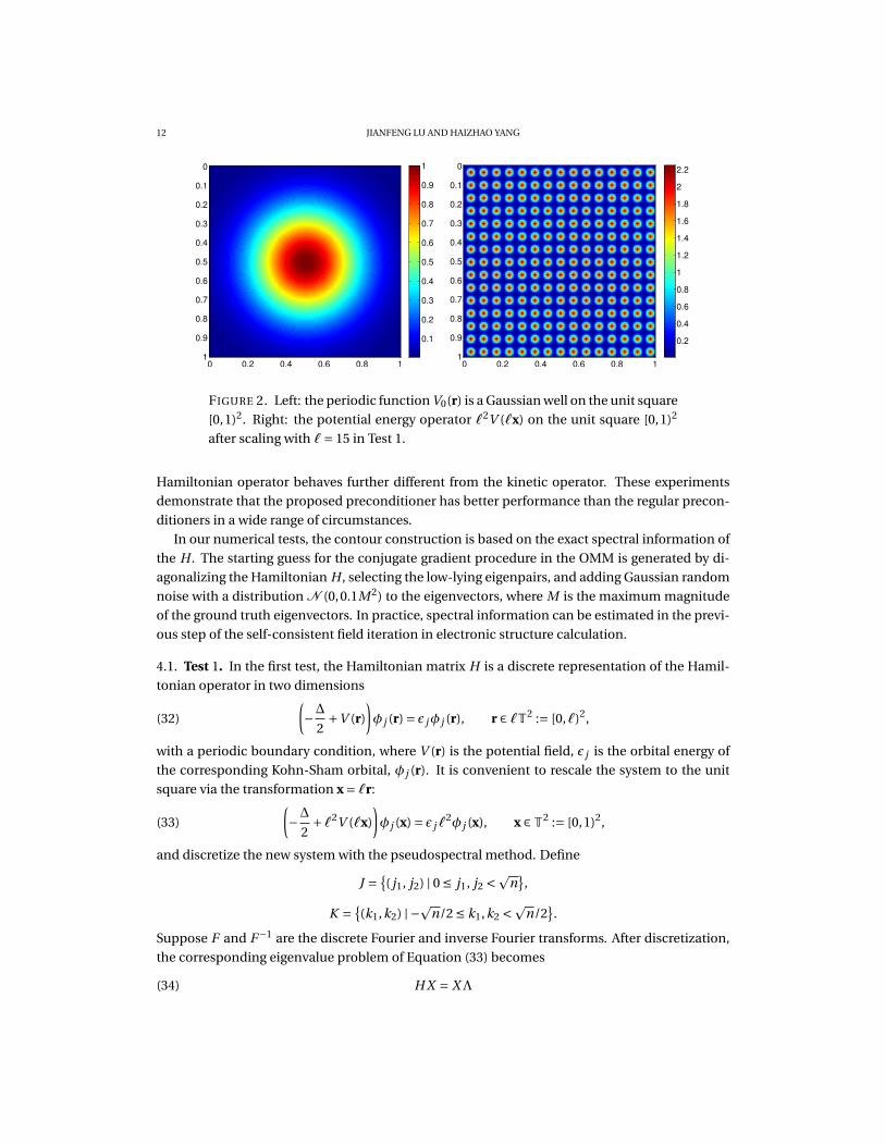
FIGURE 2. Left: the periodic function V0(r) is a Gaussian well on the unit square

[0,1)2. Right: the potential energy operator `2V (`x) on the unit square [0,1)2

after scaling with `= 15 in Test 1.

Hamiltonian operator behaves further different from the kinetic operator. These experiments

demonstrate that the proposed preconditioner has better performance than the regular precon-

ditioners in a wide range of circumstances.

In our numerical tests, the contour construction is based on the exact spectral information of

the H . The starting guess for the conjugate gradient procedure in the OMM is generated by di-

agonalizing the Hamiltonian H , selecting the low-lying eigenpairs, and adding Gaussian random

noise with a distribution N (0,0.1M 2) to the eigenvectors, where M is the maximum magnitude

of the ground truth eigenvectors. In practice, spectral information can be estimated in the previ-

ous step of the self-consistent field iteration in electronic structure calculation.

4.1. Test 1. In the first test, the Hamiltonian matrix H is a discrete representation of the Hamil-

tonian operator in two dimensions

(32)

(−∆

2+V (r)

)φ j (r) = ε jφ j (r), r ∈ `T2 := [0,`)2,

with a periodic boundary condition, where V (r) is the potential field, ε j is the orbital energy of

the corresponding Kohn-Sham orbital, φ j (r). It is convenient to rescale the system to the unit

square via the transformation x = `r:

(33)

(−∆

2+`2V (`x)

)φ j (x) = ε j`

2φ j (x), x ∈T2 := [0,1)2,

and discretize the new system with the pseudospectral method. Define

J = {( j1, j2) | 0 ≤ j1, j2 <

pn

},

K = {(k1,k2) | −pn/2 ≤ k1,k2 <

pn/2

}.

Suppose F and F−1 are the discrete Fourier and inverse Fourier transforms. After discretization,

the corresponding eigenvalue problem of Equation (33) becomes

(34) H X = XΛ


in numerical linear algebra, where H =−∆2 +V ,

−∆2= F−1 diag(2π2|k|2)k∈K F,

and

V = `2 diag

(V

(` jp

n

))j∈J

,

Λ is a diagonal matrix containing eigenvalues, and X contains the eigenvectors.

Let V0(r) be a Gaussian well on the unit square [0,1)2 (see Figure 2 left panel) and extend it

periodically with period 1 in both dimensions. In the first test, the potential term V (r) (see Figure

2 right panel) in (33) is chosen to be 0.01V0(r) so that the kinetic energy operator −∆2 dominates

the Hamiltonian operator. Hence, the spectrum of H is very close to the one of −∆2 . The precon-

ditioned OMM is applied to solve the eigenvalue problem in (34). The numerical performance

of the empirical preconditioner in (6) (denoted as TPA) and its generalization in (7) when t = 5

(denoted as gTPA), and the new preconditioner via an approximate Fermi operator projection

(denoted as SPP or PP with or without the sparsifying preconditioner, respectively), is compared

and summarized in Table 1 and Figure 3. The scaling parameter τ in the TPA and gTPA pre-

conditioner takes the value max j∑

k12 |k|2(x( j )(k))2, where x( j ) is the j th column of ground true

eigenspace F X0 and k is the two-dimensional index in K . For each Hamiltonian H with a fixed

`, 5 experiments were repeated with different random initial guesses. In this summary, some

notations are introduced and recalled as follows:

• n is the dimension of H ;

• ` is the number of cells in the domain of V (r) and each cell [0,1)2 contains a grid of size

8×8; N = `;

• cond is the condition number of the OMM;

• iter is the number of iterations in the preconditioned OMM;

• Tst is the setup time of the preconditioner; for PP and SPP, Tst is the setup time per pole.

• Tomm is the running time of the preconditioned OMM;

• Ttot = Tst +Tomm;

• d measures the distance between the column space of the ground truth eigenvectors X0

and the one of the estimated eigenvectors X by the preconditioned OMM:

d(X , X0) =∥∥X (X ∗X )−1X ∗−X0(X ∗

0 X0)−1X ∗0

∥∥∥∥X0(X ∗0 X0)−1X ∗

0

∥∥ ,

where the norm here is the entrywise `∞ norm.

The preconditioner TPA and gTPA essentially assume that the potential V (r) is negligible and

they can be implemented efficiently using the fast Fourier transform. Hence, they would be ef-

ficient in the numerical examples in Test 1 and this is supported by the results below: Tst is neg-

ligible; the preconditioned OMM converges in a few hundred iterations; the OMM returns an

eigenspace close to the ground truth, i.e., the measurement d is almost 0.

Even in this case which favors the conventional preconditioners, the new preconditioner via

an approximate Fermi operator projection (PP) is much more efficient. Even though the approx-

imation accuracy of the Fermi operator projection is low, since the tolerance of the GMRES in

computing the contour integration is large, this rough projection as a preconditioner is able to

reduce the iteration number of the OMM to 3 or 4 in all examples. The total running time of


(`,n) cond iter Tst(sec) Tomm(sec) Ttot(sec) d

TPA (3,576) 1.4e+02 5.8e+02 2.271e-03 1.669e+00 1.672e+00 9.0e-07

gTPA (3,576) 1.4e+02 5.6e+02 2.067e-03 1.695e+00 1.697e+00 7.8e-07

PP (3,576) 1.4e+02 3.0e+00 1.486e-02 1.063e-02 2.549e-02 4.4e-10

TPA (5,1600) 8.0e+02 7.4e+02 4.380e-04 6.821e+00 6.822e+00 7.5e-06

gTPA (5,1600) 8.0e+02 6.2e+02 5.310e-04 5.801e+00 5.802e+00 6.6e-06

PP (5,1600) 8.0e+02 3.0e+00 4.204e-02 3.483e-02 7.686e-02 1.6e-10

TPA (7,3136) 1.6e+03 7.7e+02 1.596e-03 2.387e+01 2.388e+01 1.0e-05

gTPA (7,3136) 1.6e+03 5.1e+02 2.333e-03 1.672e+01 1.673e+01 1.1e-05

PP (7,3136) 1.6e+03 3.0e+00 1.464e-01 1.249e-01 2.713e-01 2.5e-10

TPA (11,7744) 1.3e+03 6.6e+02 4.097e-03 1.417e+02 1.417e+02 8.8e-06

gTPA (11,7744) 1.3e+03 5.0e+02 4.640e-03 1.086e+02 1.086e+02 7.5e-06

PP (11,7744) 1.3e+03 3.0e+00 6.151e-01 7.096e-01 1.325e+00 4.5e-10

TPA (15,14400) 7.2e+03 7.2e+02 1.296e-02 6.263e+02 6.263e+02 1.1e-05

gTPA (15,14400) 7.2e+03 6.0e+02 1.245e-02 5.120e+02 5.121e+02 1.1e-05

PP (15,14400) 7.2e+03 4.0e+00 1.622e+00 3.997e+00 5.619e+00 8.9e-10

TPA (23,33856) 1.7e+04 1.1e+03 6.347e-02 7.920e+03 7.920e+03 1.1e-05

gTPA (23,33856) 1.7e+04 5.1e+02 6.488e-02 3.727e+03 3.727e+03 1.2e-05

PP (23,33856) 1.7e+04 3.0e+00 9.595e+00 2.531e+01 3.490e+01 3.3e-09

TABLE 1. Numerical results in Test 1 when V (r) = 0.01V0(r).

PP, including the setup time of the preconditioner and the running time of the OMM, is far less

than those of TPA and gTPA. The speedup factor is significant and increases as the problem gets

larger in most cases as show in Figure 3. The measurement d is much smaller than those in the

TPA and gTPA methods, which means that the solution of the OMM is more accurate than the

TPA and gTPA methods. We remark that the solutions for linear systems at different poles can

be straightforwardly parallelized, here we only use the setup time per pole in the comparison

and focus on the time spent on the iterative procedures of GMRES and OMM that can not be

parallelized. Since the GMRES with a regular preconditioner is already rather efficient and the

iteration converges less than 5 iterations, the sparsifying preconditioner is not applied in Test 1.

4.2. Test 2. In the second test, the Hamiltonian matrix H is a discrete representation of the

Hamiltonian operator in a two-dimensional Kohn-Sham equation similar to the one in (32), but

the potential energy operator is more prominent and has a local defect representing a vacancy

of the lattice, i.e., there is a random vacant cell in [0,`)2. The potential energy operator V (r) is

constructed by randomly covering a Gaussian well in V0(r) with a zero patch (see Figure 4 left

panel for an example).

The Hamiltonian matrix H is not dominated by the kinetic matrix −∆2 and hence their spectra

are different. Therefore, the performance of the regular preconditioners TPA and gTPA in Test

2 might not be as good as in Test 1. For a similar problem size n, the number of iterations in

the OMM is significantly larger than the one in Test 1. The measurement d(X , X0) is as large


6 7 8 9 10 110

0.5

1

1.5

2

2.5

3

3.5

4

4.5

5

log(n)

log

10(ite

r)

TPA

gTPA

PP

6 7 8 9 10 11

−12

−10

−8

−6

−4

−2

0

2

4

log(n)

log

10(d

)

TPA

gTPA

PP

(a) (b)

6 7 8 9 10 11

log(n)

-4

-2

0

2

4

6

8

10

12

14

log(T

tot)

TPA

gTPA

PP

3log(n)

6 7 8 9 10 1160

80

100

120

140

160

180

200

220

240

log(n)

sp

ee

d u

p f

acto

r

TPA/PP

gTPA/PP

(c) (d)

FIGURE 3. Numerical results in Test 1 when V (r) = 0.01V0(r). (a) the number of

iterations in the preconditioned OMM. (b) the measurement d(X , X0). (c) the

total running time Ttot. (d) the speedup factor of the PP method compared with

the TPA and gTPA method.

as 1e − 4 meaning that the preconditioned OMM with TPA and gTPA becomes less accurate in

revealing the true eigenspace. Since the number of vacant cells if fixed, the influence of the local

defect becomes weaker as the number of cells ` (per dimension) becomes larger. Hence, the

Hamiltonian H becomes closer to the kinetic operator and the number of iteration decreases.

This also shows that the performance of TPA and gTPA is better for Hamiltonian matrices close

to the kinetic part.

In Test 2, since the potential energy is prominent and the Hamiltonian operator behaves far

from the kinetic operator, the GMRES with an inverse shifted kinetic energy operator is not effi-

cient for solving linear systems like

(H − zk I )x = b.

The GMRES and the recently developed sparsifying preconditioner [17,31,32] are applied to solve

the above system in Test 2 and 3. The preconditioner via an approximate Fermi operator projec-

tion for the OMM is hence denoted as SPP. As shown in Table 2 and Figure 5, the performance of


0 0.2 0.4 0.6 0.8 1

0

0.1

0.2

0.3

0.4

0.5

0.6

0.7

0.8

0.9

1 0

50

100

150

200

250

0 0.2 0.4 0.6 0.8 1

0

0.1

0.2

0.3

0.4

0.5

0.6

0.7

0.8

0.9

1 0

0.5

1

1.5

2

2.5

x 104

FIGURE 4. Left: the potential energy operator V (r) with `= 16 in Test 2. Right:

the potential energy operator V (r) with `= 16 in Test 3.

the SPP method is better than the TPA and gTPA methods: the number of iteration in the OMM

is a small number of O (1); the preconditioned OMM with SPP is able to provide an eigenspace

closer to the ground truth; the SPP method is much faster and the speedup factor tends to in-

crease with n.


TPA (2,256) 3.7e+03 1.7e+03 5.514e-04 2.295e+00 2.296e+00 5.0e-05

gTPA (2,256) 3.7e+03 1.1e+03 5.518e-04 1.423e+00 1.423e+00 4.1e-05

SPP (2,256) 3.7e+03 3.0e+00 4.175e-02 4.708e-03 4.646e-02 3.1e-10

TPA (4,1024) 2.4e+05 1.3e+03 2.652e-04 7.180e+00 7.180e+00 8.5e-05

gTPA (4,1024) 2.4e+05 9.2e+02 3.680e-04 5.052e+00 5.053e+00 8.5e-05

SPP (4,1024) 2.4e+05 3.0e+00 2.074e-01 2.007e-02 2.275e-01 2.1e-09

TPA (8,4096) 9.4e+05 6.9e+02 1.098e-03 3.542e+01 3.542e+01 2.5e-05

gTPA (8,4096) 9.4e+05 5.2e+02 1.489e-03 2.680e+01 2.680e+01 2.5e-05

SPP (8,4096) 9.4e+05 3.0e+00 2.590e+00 1.965e-01 2.787e+00 1.8e-08

TPA (16,16384) 7.4e+05 8.3e+02 1.432e-02 1.096e+03 1.096e+03 1.8e-05

gTPA (16,16384) 7.4e+05 6.6e+02 1.453e-02 8.630e+02 8.630e+02 1.8e-05

SPP (16,16384) 7.4e+05 3.0e+00 3.774e+01 5.000e+00 4.274e+01 3.8e-08

TPA (32,65536) 3.1e+06 8.1e+02 1.754e-01 3.211e+04 3.211e+04 1.5e-05

gTPA (32,65536) 3.1e+06 5.7e+02 2.054e-01 2.251e+04 2.251e+04 1.5e-05

SPP (32,65536) 3.1e+06 3.0e+00 6.459e+02 1.473e+02 7.932e+02 1.5e-07

TABLE 2. Numerical results in Test 2.

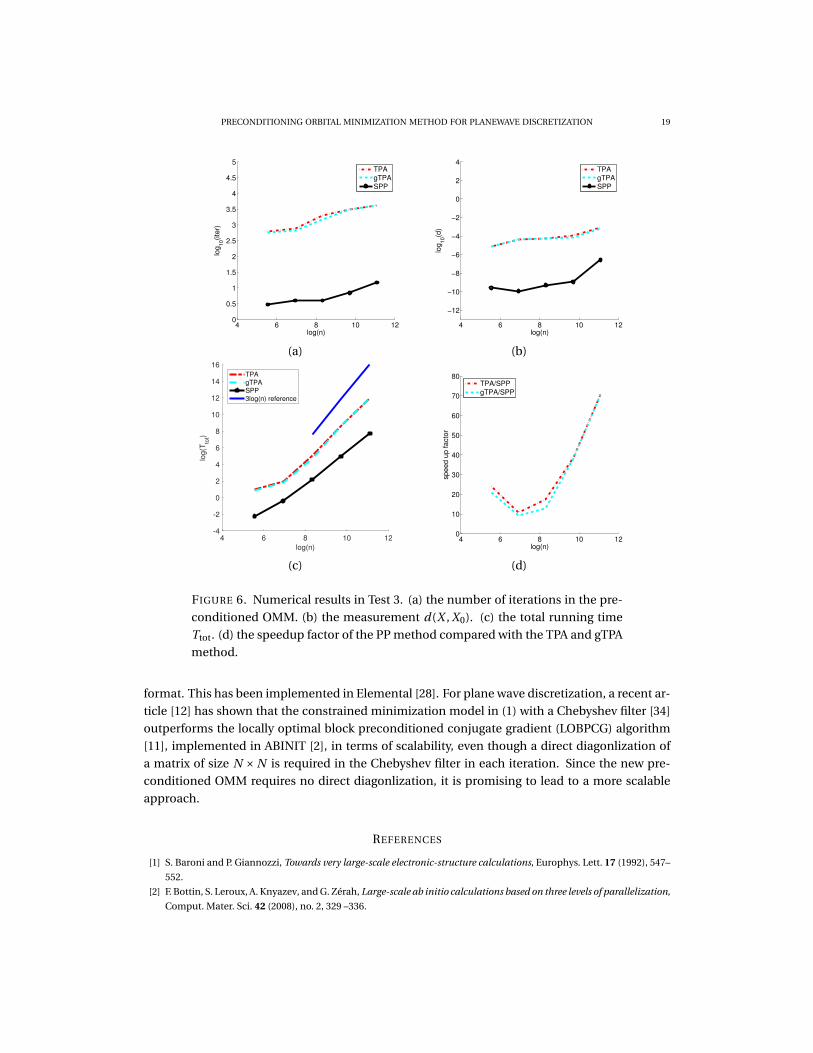
4.3. Test 3. In the last test, the potential energy operator in Test 2 is multiplied by 100 and 25%

of the cells are randomly covered by zero patches (see Figure 4 right panel for an example). Dif-

ferent from Test 2 that keeps the same number of vacant cells and varies the problem size, the


4 6 8 10 120

0.5

1

1.5

2

2.5

3

3.5

4

4.5

5

log(n)

log

10(ite

r)

TPA

gTPA

SPP

4 6 8 10 12

−12

−10

−8

−6

−4

−2

0

2

4

log(n)

log

10(d

)

TPA

gTPA

SPP

(a) (b)

4 6 8 10 12

log(n)

-4

-2

0

2

4

6

8

10

12

14

16

log(T

tot)

TPA

gTPA

SPP

3log(n) reference

4 6 8 10 125

10

15

20

25

30

35

40

45

50

log(n)

sp

ee

d u

p f

acto

r

TPA/SPP

gTPA/SPP

FIGURE 5. Numerical results in Test 2. (a) the number of iterations in the pre-

conditioned OMM. (b) the measurement d(X , X0). (c) the total running time

Ttot. (d) the speedup factor of the PP method compared with the TPA and gTPA

method.

number of vacant cells in Test 3 is proportional to the problem size so that the Hamiltonian ma-

trix H stays far away from the kinetic matrix −∆2 , and their spectra are very different. Hence, the

preconditioned OMM with TPA or gTPA is no longer efficient for all problem sizes.

As shown in Table 3 and Figure 6, the preconditioned OMM with TPA or gTPA requires thou-

sands of iterations to converge or cannot converge within the maximum number of iteration,

4000. Even if the OMM converges, it cannot return useful estimation of the eigenspace, since the

measurement d(X , X0) is too large.

In contrast, the OMM with SPP is still able to provide reasonably good estimation of the eigenspace

within O (1) iterations. Although the iteration number increases with the system size n, it remains

quite small even for large-scale problems.



TPA (2,256) 6.8e+02 6.4e+02 1.098e-03 2.602e+00 2.603e+00 7.4e-06

gTPA (2,256) 6.8e+02 5.5e+02 9.694e-04 2.244e+00 2.245e+00 7.0e-06

SPP (2,256) 6.8e+02 3.0e+00 9.940e-02 8.341e-03 1.077e-01 2.7e-10

TPA (4,1024) 2.5e+03 7.5e+02 6.446e-04 7.374e+00 7.374e+00 3.9e-05

gTPA (4,1024) 2.5e+03 6.5e+02 4.654e-04 6.401e+00 6.402e+00 3.8e-05

SPP (4,1024) 2.5e+03 4.0e+00 6.153e-01 6.153e-02 6.768e-01 1.2e-10

TPA (8,4096) 3.7e+03 2.0e+03 2.367e-03 1.562e+02 1.562e+02 4.9e-05

gTPA (8,4096) 3.7e+03 1.5e+03 2.307e-03 1.151e+02 1.151e+02 5.4e-05

SPP (8,4096) 3.7e+03 4.0e+00 8.540e+00 4.380e-01 8.978e+00 5.2e-10

TPA (16,16384) 2.4e+04 3.0e+03 2.196e-02 5.557e+03 5.557e+03 1.1e-04

gTPA (16,16384) 2.4e+04 3.0e+03 2.476e-02 5.509e+03 5.509e+03 7.8e-05

SPP (16,16384) 2.4e+04 7.0e+00 1.288e+02 1.563e+01 1.444e+02 1.1e-09

TPA (32,65536) 1.4e+05 - 2.016e-01 1.595e+05 1.595e+05 8.7e-04

gTPA (32,65536) 1.4e+05 - 2.308e-01 1.593e+05 1.593e+05 6.0e-04

SPP (32,65536) 1.4e+05 1.5e+01 1.578e+03 6.779e+02 2.256e+03 2.8e-07

TABLE 3. Numerical results in Test 3. “−" means exceeding the maximum iter-

ation number 4000.

5. CONCLUSION AND REMARKS

This paper presents a novel preconditioner for the orbital minimization method (OMM) from

planewave discretization. Once constructed, the application of the preconditioner is very ef-

ficient and the preconditioned OMM converges in O (1) iterations. Based on the approximate

Fermi operator projection, this preconditioner can be constructed efficiently via iterative matrix

solvers like GMRES with the newly developed sparsifying preconditioner. The speedup factor

of the running time compared with existing preconditioned OMMs is as large as hundreds of

times and the speedup factor tends to increase with the problem size. Numerical experiments

also show that the new preconditioned OMM is able to provide more accurate solutions than

the popular TPA preconditioner and, as a result, might reduce the number of iterations in the

self-consistent field iteration.

As for future extensions, it would be of interest to implement this new algorithm into the re-

cently developed parallel library for the OMM framework, libomm [3] and incorporate into ex-

isting electronic structure software packages. Parallelism of this new preconditioned OMM is

straightforward since the main routines of this algorithm have parallel analog in existing high

performance computing packages. Several versions of parallel FFT can be found in [25, 27]; the

computational cost per processor is less in the former one, while the latter one has a better scal-

ability and the number of processor can be O (n); a recent article [13] reduces the prefactor of the

algorithm in [27] to an optimal one in the butterfly scheme while keeping the same scalability.

The pole expansion can be embarrassingly parallelized. The last main routine, if applied, is the

scalable QR factorization used for precomputing and storing the preconditioner in a data-sparse


4 6 8 10 120

0.5

1

1.5

2

2.5

3

3.5

4

4.5

5

log(n)

log

10(ite

r)

TPA

gTPA

SPP

4 6 8 10 12

−12

−10

−8

−6

−4

−2

0

2

4

log(n)

log

10(d

)

TPA

gTPA

SPP

(a) (b)

4 6 8 10 12

log(n)

-4

-2

0

2

4

6

8

10

12

14

16

log(T

tot)

TPA

gTPA

SPP

3log(n) reference

4 6 8 10 120

10

20

30

40

50

60

70

80

log(n)

sp

ee

d u

p f

acto

r

TPA/SPP

gTPA/SPP

(c) (d)

FIGURE 6. Numerical results in Test 3. (a) the number of iterations in the pre-

conditioned OMM. (b) the measurement d(X , X0). (c) the total running time

Ttot. (d) the speedup factor of the PP method compared with the TPA and gTPA

method.

format. This has been implemented in Elemental [28]. For plane wave discretization, a recent ar-

ticle [12] has shown that the constrained minimization model in (1) with a Chebyshev filter [34]

outperforms the locally optimal block preconditioned conjugate gradient (LOBPCG) algorithm

[11], implemented in ABINIT [2], in terms of scalability, even though a direct diagonlization of

a matrix of size N × N is required in the Chebyshev filter in each iteration. Since the new pre-

conditioned OMM requires no direct diagonlization, it is promising to lead to a more scalable

approach.

REFERENCES

[1] S. Baroni and P. Giannozzi, Towards very large-scale electronic-structure calculations, Europhys. Lett. 17 (1992), 547–

552.

[2] F. Bottin, S. Leroux, A. Knyazev, and G. Zérah, Large-scale ab initio calculations based on three levels of parallelization,

Comput. Mater. Sci. 42 (2008), no. 2, 329 –336.


[3] F. Corsetti, The orbital minimization method for electronic structure calculations with finite-range atomic basis sets,

Comput. Phys. Commun. 185 (2014), 873–883.

[4] A. Damle, L. Lin, and L. Ying, Pole expansion for solving a type of parametrized linear systems in electronic structure

calculations, SIAM J. Sci. Comput. 36 (2014), no. 6, A2929–A2951.

[5] J. W. Demmel, L. Grigori, M. Gu, and H. Xiang, Communication avoiding rank revealing QR factorization with column

pivoting, SIAM J. Matrix Anal. Appl. 36 (2015), no. 1, 55–89.

[6] A. George, Nested dissection of a regular finite element mesh, SIAM J. Numer. Anal. 10 (1973), 345–363.

[7] S. Goedecker, Low complexity algorithms for electronic structure calculations, J. Comput. Phys. 118 (1995), no. 2, 261

–268.

[8] S. Goedecker, Linear scaling electronic structure methods, Rev. Mod. Phys. 71 (1999), 1085–1123.

[9] N. Hale, N. J. Higham, and L. N. Trefethen, Computing aα, log(a), and related matrix functions by contour integrals,

SIAM J. Numer. Anal. 46 (2008), no. 5, 2505–2523.

[10] N. Halko, P. G. Martinsson, and J. A. Tropp, Finding structure with randomness: Probabilistic algorithms for construct-

ing approximate matrix decompositions, SIAM review 53 (2011), no. 2, 217–288.

[11] A. V. Knyazev, Toward the optimal preconditioned eigensolver: Locally optimal block preconditioned conjugate gradi-

ent method, SIAM J. Sci. Comput. 23 (2001), no. 2, 517–541.

[12] A. Levitt and M. Torrent, Parallel eigensolvers in plane-wave density functional theory, Comput. Phys. Commun. 187

(2015), 98 –105.

[13] Y. Li and H. Yang, Interpolative butterfly factorization, 2016. preprint.

[14] L. Lin, J. Lu, L. Ying, R. Car, and W. E, Fast algorithm for extracting the diagonal of the inverse matrix with application

to the electronic structure analysis of metallic systems, Comm. Math. Sci. 7 (2009), 755–777.

[15] L. Lin, J. Lu, L. Ying, and W. E, Pole-based approximation of the Fermi-Dirac function, Chin. Ann. Math. Ser. B 30

(2009), no. 6, 729–742.

[16] L. Lin, C. Yang, J. Lu, L. Ying, and W. E, A fast parallel algorithm for selected inversion of structured sparse matrices

with application to 2d electronic structure calculations, SIAM J. Sci. Comput. 33 (2011), no. 3, 1329–1351.

[17] J. Lu and L. Ying, Sparsifying preconditioner for soliton calculations, J. Comput. Phys. in press.

[18] P. G. Martinsson, Blocked rank-revealing QR factorizations: How randomized sampling can be used to avoid single-

vector pivoting, 2015. preprint.

[19] F. Mauri and G. Galli, Electronic structure calculations and molecular dynamics simulations with linear system-size

scaling, Phys. Rev. B 50 (1994), 4316–4326.

[20] F. Mauri, G. Galli, and R. Car, Orbital formulation for electronic-structure calculations with linear system-size scaling,

Phys. Rev. B 47 (1993), 9973–9976.

[21] P. Ordejón, D. A. Drabold, M. P. Grumbach, and R. M. Martin, Unconstrained minimization approach for electronic

computations that scales linearly with system size, Phys. Rev. B 48 (1993), 14646–14649.

[22] P. Ordejón, D. A. Drabold, R. M. Martin, and M. P. Grumbach, Linear system-size scaling methods for electronic-

structure calculations, Phys. Rev. B 51 (1995), 1456–1476.

[23] M.C. Payne, M.P. Teter, D.C. Allan, T.A. Arias, and J.D. Joannopoulos, Iterative minimization techniques for ab initio

total-energy calculations: molecular dynamics and conjugate gradients, Rev. Mod. Phys. 64 (1992), 1045–1097.

[24] B. G. Pfrommer, J. Demmel, and H. Simon, Unconstrained energy functionals for electronic structure calculations, J.

Comput. Phys. 150 (1999), 287–298.

[25] M. Pippig, PFFT: An extension of FFTW to massively parallel architectures, SIAM J. Sci. Comput. 35 (2013), no. 3,

C213–C236.

[26] E. Polizzi, Density-matrix-based algorithm for solving eigenvalue problems, Phys. Rev. B 79 (2009), 115112.

[27] J. Poulson, L. Demanet, N. Maxwell, and L. Ying, A parallel butterfly algorithm, SIAM J. Sci. Comput. 36 (2014), no. 1,

C49–C65.

[28] J. Poulson, B. Marker, R. A. van de Geijn, J. R. Hammond, and N. A. Romero, Elemental: A new framework for dis-

tributed memory dense matrix computations, ACM Trans. Math. Softw. 39 (2013), no. 2, 13:1–13:24.

[29] Y. Saad and M. H. Schultz, GMRES: a generalized minimal residual algorithm for solving nonsymmetric linear systems,

SIAM J. Sci. Statist. Comput. 7 (1986), 856–869.

[30] M. P. Teter, M. C. Payne, and D. C. Allan, Solution of Schrödinger’s equation for large systems, Phys. Rev. B 40 (1989),

12255–12263.


[31] L. Ying, Sparsifying preconditioner for pseudospectral approximations of indefinite systems on periodic structures,

Multiscale Model. Simul. 13 (2015), no. 2, 459–471.

[32] L. Ying, Sparsifying preconditioner for the Lippmann-Schwinger equation, Multiscale Model. Simul. 13 (2015), no. 2,

644–660.

[33] Y. Zhou, J. R. Chelikowsky, X. Gao, and A. Zhou, On the “preconditioning” function used in planewave DFT calcula-

tions and its generalization, Commun. Comput. Phys. 18 (2015), 167–179.

[34] Y. Zhou, Y. Saad, M. L. Tiago, and J. R. Chelikowsky, Self-consistent-field calculations using Chebyshev-filtered sub-

space iteration, J. Comput. Phys. 219 (2006), no. 1, 172 –184.

DEPARTMENT OF MATHEMATICS, DEPARTMENT OF PHYSICS, AND DEPARTMENT OF CHEMISTRY, DUKE UNIVERSITY,

BOX 90320, DURHAM NC 27708, USA

E-mail address: [email protected]

DEPARTMENT OF MATHEMATICS, DUKE UNIVERSITY, BOX 90320, DURHAM NC 27708, USA

E-mail address: [email protected]

Documents

PRECONDITIONING ORBITAL MINIMIZATION METHOD FOR …matyh/publications/sppOMM.pdf · A natural question is whether more ... The OMM method is highly efﬁcient in each iteration,