Embed Size (px)
Citation preview

Geoscience Laser Altimeter System (GLAS)
Algorithm Theoretical Basis Document Version 2.2
PRECISION ORBIT DETERMINATION (POD)
Prepared by:
H. J. Rim B. E. Schutz
Center for Space Research The University of Texas at Austin
October 2002

TABLE OF CONTENTS
1.0 INTRODUCTION..................................................................................................................... 1
1.1 BACKGROUND ....................................................................................................................... 1
1.2 THE POD PROBLEM............................................................................................................... 2
1.3 GPS-BASED POD.................................................................................................................... 2
1.3.1 Historical Perspective ..................................................................................................... 3
1.3.2 GPS-based POD Strategies............................................................................................. 4
1.4 OUTLINE ................................................................................................................................. 6
2.0 OBJECTIVE.............................................................................................................................. 7
3.0 ALGORITHM DESCRIPTION: ORBIT ............................................................................... 8
3.1 ICESAT/GLAS ORBIT DYNAMICS OVERVIEW.................................................................... 8
3.2 EQUATIONS OF MOTION, TIME AND COORDINATE SYSTEMS .......................................... 8
3.2.1 Time System..................................................................................................................... 9
3.2.2 Coordinate System......................................................................................................... 10
3.3 GRAVITATIONAL FORCES................................................................................................... 11
3.3.1 Geopotential .................................................................................................................. 11
3.3.2 Solid Earth Tides ........................................................................................................... 13
3.3.3 Ocean Tides................................................................................................................... 14
3.3.4 Rotational Deformation................................................................................................. 15
3.3.5 N-Body Perturbation ..................................................................................................... 17
3.3.6 General Relativity.......................................................................................................... 18
3.4 NONGRAVITATIONAL FORCES........................................................................................... 19
3.4.1 Atmospheric Drag ......................................................................................................... 20

2
3.4.2 Solar Radiation Pressure .............................................................................................. 22
3.4.3 Earth Radiation Pressure.............................................................................................. 23
3.4.4 Thermal Radiation Perturbation ................................................................................... 25
3.4.5 GPS Solar Radiation Pressure Models ......................................................................... 26
3.4.6 ICESat/GLAS "Box-Wing" Model ................................................................................. 28
3.5 EMPIRICAL FORCES............................................................................................................. 29
3.5.1 Empirical Tangential Perturbation ............................................................................... 29
3.5.2 Once-per Revolution RTN Perturbation........................................................................ 30
4.0 ALGORITHM DESCRIPTION: MEASUREMENTS ........................................................ 32
4.1 ICESAT/GLAS MEASUREMENTS OVERVIEW ................................................................... 32
4.2 GPS MEASUREMENT MODEL ............................................................................................. 32
4.2.1 Code Pseudorange Measurement.................................................................................. 32
4.2.2 Phase Pseudorange Measurement ................................................................................ 33
4.2.3 Double-Differenced High-Low Phase Pseudorange Measurement .............................. 37
4.2.4 Corrections.................................................................................................................... 41
4.2.4.1 Propagation Delay ................................................................................................. 41
4.2.4.2 Relativistic Effect .................................................................................................. 43
4.2.4.3 Phase Center Offset ............................................................................................... 44
4.2.4.4 Ground Station Related Effects ............................................................................. 44
4.2.5 Measurement Model Partial Derivatives ...................................................................... 46
4.3 SLR MEASUREMENT MODEL ............................................................................................. 49
4.3.1 Range Model and Corrections ...................................................................................... 49
3
4.3.2 Measurement Model Partial Derivatives ...................................................................... 50
5.0 ALGORITHM DESCRIPTION: ESTIMATION ................................................................ 51
5.1 LEAST SQUARES ESTIMATION ........................................................................................... 51
5.2 PROBLEM FORMULATION FOR MULTI-SATELLITE ORBIT DETERMINATION ............... 56
5.3 OUTPUT ................................................................................................................................ 68
6.0 IMPLEMENTATION CONSIDERATIONS ....................................................................... 69
6.1 POD SOFTWARE SYSTEM ................................................................................................... 69
6.1.1 Ancillary Inputs ............................................................................................................. 70
6.2 POD PRODUCTS ................................................................................................................... 70
6.3 ICESAT/GLAS ORBIT AND ATTITUDE .............................................................................. 71
6.4 POD ACCURACY ASSESSMENT.......................................................................................... 72
6.5 POD PROCESSING STRATEGY ............................................................................................ 74
6.5.1 Assumptions and Issues ................................................................................................. 74
6.5.2 GPS Data Preprocessing............................................................................................... 74
6.5.3 GPS Orbit Determination.............................................................................................. 76
6.5.4 Estimation Strategy ....................................................................................................... 77
6.6 POD PLANS .......................................................................................................................... 77
6.6.1 Pre-Launch POD Activities........................................................................................... 77
6.6.1.1 Standards ............................................................................................................... 78
6.6.1.2 Gravity Model Improvements ............................................................................... 81
6.6.1.3 Non-Gravitational Model Improvements .............................................................. 81
6.6.1.4 Measurement Model Developments ...................................................................... 83
4
6.6.1.5 Preparation for Operational POD .......................................................................... 84
6.6.1.6 Software Comparison ............................................................................................ 84
6.6.1.7 POD Accuracy Assessment ................................................................................... 85
6.6.2 Post-Launch POD Activities.......................................................................................... 85
6.6.2.1 Verification/Validation Period .............................................................................. 85
6.6.2.2 POD Product Validation........................................................................................ 87
6.6.2.3 POD Reprocessing ................................................................................................ 87
6.7 COMPUTATIONAL: CPU, MEMORY AND DISK STORAGE ................................................ 88
7.0 BIBLIOGRAPHY ................................................................................................................... 91

1
1.0 INTRODUCTION
1.1 Background
The EOS ICESat mission is scheduled for launch on July 2001. Three
major science objectives of this mission are: (1) to measure long-term changes in the
volumes (and mass) of the Greenland and Antarctic ice sheets with sufficient
accuracy to assess their impact on global sea level, and to measure seasonal and
interannual variability of the surface elevation, (2) to make topographic
measurements of the Earth's land surface to provide ground control points for
topographic maps and digital elevation models, and to detect topographic change, and
(3) to measure the vertical structure and magnitude of cloud and aerosol parameters
that are important for the radiative balance of the Earth-atmosphere system, and
directly measure the height of atmospheric transition layers. The spacecraft features
the Geoscience Laser Altimeter System (GLAS), which will measure a laser pulse
round-trip time of flight, emitted by the spacecraft and reflected by the ice sheet or
land surface. This laser altimeter measurement provides height of the GLAS
instrument above the ice sheet. The geocentric height of the ice surface is computed
by differencing the altimeter measurement from the satellite height, which is
computed from Precision Orbit Determination (POD) using satellite tracking data.
To achieve the science objectives, especially for measuring the ice-sheet
topography, the position of the GLAS instrument should be known with an accuracy
of 5 and 20 cm in radial and horizontal components, respectively. This knowledge
will be acquired from data collected by the on-board GPS receiver and ground GPS
receivers and from the ground-based satellite laser ranging (SLR) data. GPS data will

2
be the primary tracking data for the ICESat/GLAS POD, and SLR data will be used
for POD validation.
1.2 The POD Problem
The problem of determining an accurate ephemeris for an orbiting satellite
involves estimating the position and velocity of the satellite from a sequence of
observations, which are a function of the satellite position, and velocity. This is
accomplished by integrating the equations of motion for the satellite from a reference
epoch to each observation time to produce predicted observations. The predicted
observations are differenced from the true observations to produce observation
residuals. The components of the satellite state (satellite position and velocity and
the estimated force and measurement model parameters) at the reference epoch are
then adjusted to minimize the observation residuals in a least square sense. Thus, to
solve the orbit determination problem, one needs the equations of motion describing
the forces acting on the satellite, the observation-state relationship describing the
relation of the observed parameters to the satellite state, and the least squares
estimation algorithm used to obtain the estimate.
1.3 GPS-based POD
Since the earliest concepts, which led to the development of the Global
Positioning System (GPS), it has been recognized that this system could be used for
tracking low Earth orbiting satellites. Compared to the conventional ground-based
tracking systems, such as the satellite laser ranging or Doppler systems, the GPS

3
tracking system has the advantage of providing continuous tracking of a low satellite
with high precision observations of the satellite motion with a minimal number of
ground stations. The GPS tracking system for POD consists of a GPS flight receiver,
a global GPS tracking network, and a ground data processing and control system.
1.3.1 Historical Perspective
The GPS tracking system has demonstrated its capability of providing
high precision POD products through the GPS flight experiment on TOPEX/Poseidon
(T/P) [Melbourne et al., 1994]. Precise orbits computed from the GPS tracking data
[Yunck et al., 1994; Christensen et al., 1994; Schutz et al., 1994] are estimated to
have a radial orbit accuracy comparable to or better than the precise orbit
ephemerides (POE) computed from the combined SLR and DORIS tracking data
[Tapley et al., 1994] on T/P. When the reduced-dynamic orbit determination
technique was employed with the GPS data, which includes process noise
accelerations that absorb dynamic model errors after fixing all dynamic model
parameters from the fully dynamic approach, there is evidence to suggest that the
radial orbit accuracy is better than 3 cm [Bertiger et al., 1994].
While GPS receivers have flown on missions prior to T/P, such as
Landsat-4 and -5, and Extreme Ultraviolet Explorer, the receivers were single
frequency and had high level of ionospheric effects relative to the dual frequency T/P
receiver. In addition, the satellite altitudes were 700 km and 500 km, respectively,
and the geopotential models available for POD, as they are today, had large errors for
4
such altitudes. As a result, sub-decimeter radial orbit accuracy could not be achieved
for these satellites.
Through the GPS flight experiment on T/P several important lessons on
GPS-based POD have been learned. Those include: 1) GPS Demonstration Receiver
(GPS/DR) on T/P provides continuous, global, and high precision GPS observable.
2) GPS-based POD produces T/P radial orbit accuracy similar or better than
SLR/DORIS. 3) Gravity tuning using GPS measurement was effective [Tapley et al.,
1996]. 4) Both reduced-dynamic technique and dynamic approach with extensive
parameterization have been shown to reduce orbit errors caused by mismodeling of
satellite forces.
1.3.2 GPS-based POD Strategies
Several different POD approaches are available using GPS measurements.
Those include the kinematic or geometric approach, dynamic approach, and the
reduced-dynamic approach.
The kinematic or geometric approach does not require the description of
the dynamics except for possible interpolation between solution points for the user
satellite, and the orbit solution is referenced to the phase center of the on-board GPS
antenna instead of the satellite's center of mass. Yunck and Wu [1986] proposed a
geometric method that uses the continuous record of satellite position changes
obtained from the GPS carrier phase to smooth the position measurements made with
pseudorange. This approach assumes the accessibility of P-codes at both the L1 and
L2 frequencies. Byun [1998] developed a kinematic orbit determination algorithm

5
using double- and triple-differenced GPS carrier phase measurements. Kinematic
solutions are more sensitive to geometrical factors, such as the direction of the GPS
satellites and the GPS orbit accuracy, and they require the resolution of phase
ambiguities.
The dynamic orbit determination approach [Tapley, 1973] requires precise
models of the forces acting on user satellite. This technique has been applied to many
successful satellite missions and has become the mainstream POD approach.
Dynamic model errors are the limiting factor for this technique, such as the
geopotential model errors and atmospheric drag model errors, depending on the
dynamic environment of the user satellite. With the continuous, global, and high
precision GPS tracking data, dynamic model parameters, such as geopotential
parameters, can be tuned effectively to reduce the effects of dynamic model error in
the context of dynamic approach. The dense tracking data also allows for the
frequent estimation of empirical parameters to absorb the effects of unmodeled or
mismodeled dynamic error.
The reduced-dynamic approach [Wu et al., 1987] uses both geometric and
dynamic information and weighs their relative strength by solving for local geometric
position corrections using a process noise model to absorb dynamic model errors.
Note that the adopted approach for ICESat/GLAS POD is the dynamic
approach with gravity tuning and the reduced-dynamic solutions will be used for
validation of the dynamic solutions.
6
1.4 Outline
This document describes the algorithms for the precise orbit determination
(POD) of ICESat/GLAS. Chapter 2 describes the objective for ICESat/GLAS POD
algorithm. Chapter 3 summarizes the dynamic models, and Chapter 4 describes the
measurement models for ICESat/GLAS. Chapter 5 describes the least squares
estimation algorithm and the problem formulation for multi-satellite orbit
determination problem. Chapter 6 summarizes the implementation considerations for
ICESat/GLAS POD algorithms.

7
2.0 OBJECTIVE
The objective of the POD algorithm is to determine an accurate position of
the center of mass of the spacecraft carrying the GLAS instrument. This position
must be expressed in an appropriate Earth-fixed reference frame, such as the
International Earth Rotation Service (IERS) Terrestrial Reference Frame (ITRF), but
for some applications the position vector must be given in a non-rotating frame, the
IERS Celestial Reference Frame (ICRF). Thus, the POD algorithm will provide a
data product that consists of time and the (x, y, z) position (ephemeris) of the
spacecraft/GLAS center of mass in both the ITRF and the ICRF. The ephemeris will
be provided at an appropriate time interval, e.g., 30 sec and interpolation algorithms
will enable determination of the position at any time to an accuracy comparable to the
numerical integration accuracy. Furthermore, the transformation matrix between
ICRF and ITRF will be provided from the POD, along with interpolation algorithm.
8
3.0 ALGORITHM DESCRIPTION: Orbit
3.1 ICESat/GLAS Orbit Dynamics Overview
Mathematical models employed in the equations of motion to describe the
motion of ICESat/GLAS can be divided into three categories: 1) the gravitational
forces acting on ICESat/GLAS consist of Earth’s geopotential, solid earth tides,
ocean tides, planetary third-body perturbations, and relativistic accelerations; 2) the
non-gravitational forces consist of drag, solar radiation pressure, earth radiation
pressure, and thermal radiation acceleration; and 3) empirical force models that are
employed to accommodate unmodeled or mismodeled forces. In this chapter, the
dynamic models are described along with the time and reference coordinate systems.
3.2 Equations of Motion, Time and Coordinate Systems
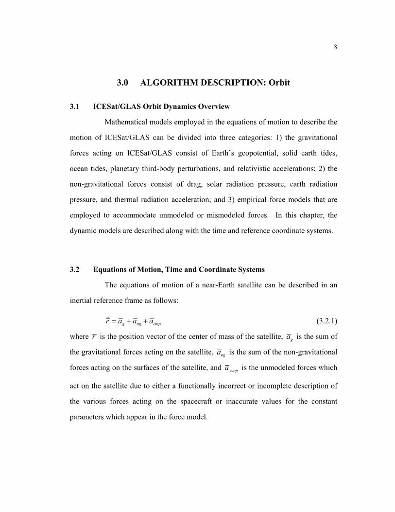
The equations of motion of a near-Earth satellite can be described in an
inertial reference frame as follows:
g ng empr a a a= + + (3.2.1)
where r is the position vector of the center of mass of the satellite, ga is the sum of
the gravitational forces acting on the satellite, nga is the sum of the non-gravitational
forces acting on the surfaces of the satellite, and empa is the unmodeled forces which
act on the satellite due to either a functionally incorrect or incomplete description of
the various forces acting on the spacecraft or inaccurate values for the constant
parameters which appear in the force model.

9
3.2.1 Time System
Several time systems are required for the orbit determination problem.
From the measurement systems, satellite laser ranging measurements are usually
time-tagged in UTC (Coordinated Universal Time) and GPS measurements are time-
tagged in GPS System Time (referred to here as GPS-ST). Although both UTC and
GPS-ST are based on atomic time standards, UTC is loosely tied to the rotation of the
Earth through the application of "leap seconds" to keep UT1 and UTC within a
second. GPS-ST is continuous to avoid complications associated with a
discontinuous time scale [Milliken and Zoller, 1978]. Leap seconds are introduced on
January 1 or July 1, as required. The relation between GPS-ST and UTC is
GPS-ST = UTC + n (3.2.2)
where n is the number of leap seconds since January 6, 1980. For example, the
relation between UTC and GPS-ST in mid-July, 1999, was GPS-ST = UTC + 13 sec.
The independent variable of the near-Earth satellite equations of motion (Eq. 3.2.1) is
typically TDT (Terrestrial Dynamical Time), which is an abstract, uniform time scale
implicitly defined by equations of motion. This time scale is related to the TAI
(International Atomic Time) by the relation
TDT = TAI + 32.184s. (3.2.3)
The planetary ephemerides are usually given in TDB (Barycentric Dynamical Time)
scale, which is also an abstract, uniform time scale used as the independent variable
for the ephemerides of the Moon, Sun, and planets. The transformation from the
TDB time to the TDT time with sufficient accuracy for most application has been

10
given by Moyer [1981]. For a near-Earth application like ICESat/GLAS, it is
unnecessary to distinguish between TDT and TDB. New time systems are under
discussion by the International Astronomical Union. This document will be updated
with these time systems, as appropriate.
3.2.2 Coordinate System
The inertial reference system adopted for Eq. 3.2.1 for the dynamic model
is the ICRF geocentric inertial coordinate system, which is defined by the mean
equator and vernal equinox at Julian epoch 2000.0. The Jet Propulsion Laboratory
(JPL) DE-405 planetary ephemeris [Standish, 1998], which is based on the ICRF
inertial coordinate system, has been adopted for the positions and velocities of the
planets with the coordinate transformation from barycentric inertial to geocentric
inertial.
Tracking station coordinates, atmospheric drag perturbations, and
gravitational perturbations are usually expressed in the Earth fixed, geocentric,
rotating system, which can be transformed into the ICRF reference frame by
considering the precession and nutation of the Earth, its polar motion, and UT1
transformation. The 1976 International Astronomical Union (IAU) precession
[Lieske et al., 1977; Lieske, 1979] and the 1980 IAU nutation formula [Wahr, 1981b;
Seidelmann, 1982] with the correction derived from VLBI analysis [Herring et al.,
1991] will be used as the model of precession and nutation of the Earth. Polar motion
and UT1-TAI variations were derived from Lageos (Laser Geodynamics Satellite)
laser ranging analysis [Tapley et al., 1985; Schutz et al., 1988]. Tectonic plate

11
motion for the continental mass on which tracking stations are affixed has been
modeled based on the AM0-2 model [Minster and Jordan, 1978; DeMets et al., 1990;
Watkins, 1990]. Yuan [1991] provides additional detailed discussion of time and
coordinate systems in the satellite orbit determination problem.
3.3 Gravitational Forces
The gravitational forces can be expressed as:
ag = Pgeo + Pst + Pot + Prd + Pn + Prel (3.3.1)
where
Pgeo = perturbations due to the geopotential of the Earth
Pst = perturbations due to the solid Earth tides
Pot = perturbations due to the ocean tides
Prd = perturbations due to the rotational deformation
Pn = perturbations due to the Sun, Moon and planets
Prel = perturbations due to the general relativity
3.3.1 Geopotential
The perturbing forces of the satellite due to the gravitational attraction of
the Earth can be expressed as the gradient of the potential, U, which satisfies the
Laplace equation, ∇2U = 0:
12
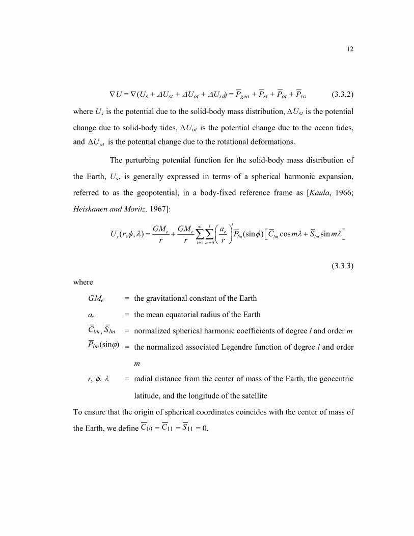
∇U = ∇(Us + ∆Ust + ∆Uot + ∆Urd) = Pgeo + Pst + Pot + Prd (3.3.2)
where Us is the potential due to the solid-body mass distribution, ∆Ust is the potential
change due to solid-body tides, ∆Uot is the potential change due to the ocean tides,
and rdU∆ is the potential change due to the rotational deformations.
The perturbing potential function for the solid-body mass distribution of
the Earth, Us, is generally expressed in terms of a spherical harmonic expansion,
referred to as the geopotential, in a body-fixed reference frame as [Kaula, 1966;
Heiskanen and Moritz, 1967]:
1 0
( , , ) (sin ) cos sinll
e e es lm lm lm
l m
GM GM aU r P C m S mr r r
φ λ φ λ λ∞
= =
= + + ∑∑
(3.3.3)
where
GMe = the gravitational constant of the Earth
ae = the mean equatorial radius of the Earth
Clm , Slm = normalized spherical harmonic coefficients of degree l and order m
Plm(sinϕ) = the normalized associated Legendre function of degree l and order
m
r, φ, λ = radial distance from the center of mass of the Earth, the geocentric
latitude, and the longitude of the satellite
To ensure that the origin of spherical coordinates coincides with the center of mass of
the Earth, we define C10 = C11 = S11 = 0.

13
3.3.2 Solid Earth Tides
Since the Earth is a non-rigid elastic body, its mass distribution and the
shape will be changed under the gravitational attraction of the perturbing bodies,
especially the Sun and the Moon. The temporal variation of the free space
geopotential induced from solid Earth tides can be expressed as a change in the
external geopotential by the following expression [Wahr, 1981a; Dow, 1988; Casotto,
1989].
1 3(3)
( ) 0 22
2 0 ( , )
( , ) ( , )k k
l lli l le e e
st k k m k ml m k l me
GM a aU H e k Y k Yr ra
χ φ λ φ λ+ +
Θ + + +
= =
∆ = +
∑∑ ∑
(3.3.4)
where
(2 1) ( )!( , ) ( 1) (sin )4 ( )!
m m iml lm
l l mY P el m
λφ λ φπ+ −
= −+
(sin )lmP φ = the unnormalized associated Legendre function of degree l and
order m
Hk = the frequency dependent tidal amplitude in meters (provided in
Cartwright and Tayler [1971] and Cartwright and Edden
[1973])
Θk , χk = Doodson argument and phase correction for constituent k
(χk = 0, if l-m is even; χk = 2π
− , if l-m is odd)
kk0, kk
+ = Love numbers for tidal constituent k
r, φ, λ = geocentric body-fixed coordinates of the satellite

14
The summation over k(l,m) means that each different l, m combination has a unique
list of tidal frequencies, k, to sum over.
The tidally induced variations in the Earth’s external potential can be
expressed as variations in the spherical harmonic geopotential coefficients [Eanes et
al. 1983].
0
0
cos ,( 1)sin ,4 (2 )
mk
lm k kk ke m
l m evenC k H
l m odda π δΘ −−
∆ = Θ −− ∑
0
0
sin ,( 1)cos ,4 (2 )
mk
lm k kk ke m
l m evenS k H
l m odda π δ− Θ −−
∆ = Θ −− ∑ (3.3.5)
where δ0m is the Kronecker delta; ∆Clm and ∆Slm are the time-varying geopotential
coefficients providing the spatial description of the luni-solar tidal effect.
3.3.3 Ocean Tides
The oceanic tidal perturbations due to the attraction of the Sun and the
Moon can be expressed as variations in the spherical harmonic geopotential
coefficients. The temporal variation of the free space geopotential induced from the
ocean tide deformation, ∆Uot , can be expressed as [Eanes et al., 1983]
1'
0 0
142 1
lll e
ot w ek l m
k aU G al r
π ρ+∞ −
= = +
+ ∆ = + ∑∑∑∑
× Cklm± cos(Θk±mλ) + Sklm
± sin(Θk±mλ) Plm(sinφ) (3.3.6)

15
where ρw is the mean density of sea water, k is the ocean tide constituent index, kl' is
the load Love number of degree l, Cklm± and Sklm
± are the unnormalized prograde and
retrograde tide coefficients, and Θk is the Doodson argument for constituent k.
The above variations in the Earth’s external potential due to the ocean tide
can be expressed as variations in the spherical harmonic geopotential coefficients as
follows [Eanes et al. 1983].
lm lm klmk
C F A∆ = ∑
lm lm klmk
S F B∆ = ∑ (3.3.7)
where Flm , Aklm , and Bklm are defined as
Flm = 4πae2ρw
Me
(l+m)!(l-m)!(2l+1)(2-δ0m)
1+kl'
2l+1 (3.3.8)
and
Aklm
Bklm =
(Cklm+ + Cklm
- )
(Sklm+ - Sklm
- ) cosΘk +
(Sklm+ + Sklm
- )
(Cklm- - Cklm
+ ) sinΘk (3.3.9)
3.3.4 Rotational Deformation
Since the Earth is elastic and includes a significant fluid component,
changes in the angular velocity vector will produce a variable centrifugal force,
which consequently deforms the Earth. This deformation, which is called “rotational
deformation”, can be expressed as the change of the centrifugal potential, Uc
[Lambeck, 1980] given by

16
Uc = 13
ω2r2 + ∆Uc (3.3.10)
where
∆Uc = r2
6 (ω1
2+ω22-2ω3
2) P20(sinφ)
- r2
3 (ω1ω3cosλ + ω2ω3sinλ) P21(sinφ)
+ r2
12 (ω2
2-ω12)cos2λ - 2ω1ω2sin2λ P22(sinφ) (3.3.11)
and ω1 = Ωm1, ω2 = Ωm2, ω3 = Ω (1+m3), and ω2 = (ω12+ω2
2+ω32). Ω is the mean
angular velocity of the Earth, mi are small dimensionless quantities which are related
to the polar motion and the Earth rotation parameters by the following expressions:
m1 = xp
m2 = - yp (3.3.12)
m3 = d (UT1-TAI)d (TAI)
The first term of Eq. (3.3.10) is negligible in the variation of the
geopotential, thereby the variation of the free space geopotential outside of the Earth
due to the rotational deformation can be written as
∆Urd = aer
3k2 ∆Uc(ae) (3.3.13)
The above variations in the Earth’s external potential due to the rotational
deformation can be expressed as variations in the spherical harmonic geopotential
coefficients as follows.
∆C20 = ae3
6GMe m12+m22-2(1+m3)2 Ω 2k2 ≈ -ae3
3GMe (1+2m3)Ω 2k2

17
∆C21 = -ae3
3GMe m1(1+m3)Ω 2k2 ≈ -ae3
3GMe m1Ω 2k2
∆S21 = -ae3
3GMe m2(1+m3)Ω 2k2 ≈ -ae3
3GMe m2Ω 2k2 (3.3.14)
∆C22 = ae3
12GMe (m22-m12)Ω 2k2 ≈ 0
∆S22 = -ae3
6GMe (m2m1)Ω 2k2 ≈ 0
As a consequence of Eqs. (3.3.2), (3.3.3), (3.3.4), (3.3.6), and (3.3.13), the
resultant gravitational potential for the Earth can be expressed as
( )1 0
( , , ) sinll
e e elm
l m
GM GM aU r Pr r r
φ λ φ∞
= =
= +
∑∑
× Clm+∆Clm cosmλ + Slm+∆Slm sinmλ (3.3.15)
where both the solid Earth and oceans contribute to the periodic variations ∆Clm and
∆Slm .
3.3.5 N-Body Perturbation
The gravitational perturbations of the Sun, Moon and other planets can be
modeled with sufficient accuracy using point mass approximations. In the geocentric
inertial coordinate system, the N-body accelerations can be expressed as:
3 3i i
n ii i i
rP GMr
∆= − ∆
∑ (3.3.16)
where

18
G = the universal gravitational constant
Mi = mass of the i-th perturbing body
ri = position vector of the i-th perturbing body in geocentric inertial
coordinates
∆i = position vector of the i-th perturbing body with respect to the
satellite
The values of ri can be obtained from the Jet Propulsion Laboratory Development
Ephemeris-405 (JPL DE-405) [Standish, 1998].
3.3.6 General Relativity
The general relativistic perturbations on the near-Earth satellite can be
modeled as [Huang et al., 1990; Ries et al., 1988],
Prel = GMec2r3
(2β+2γ) GMer - γ(r ⋅ r) r + (2+2γ) (r ⋅ r) r
+ 2 (Ω × r) (3.3.17)
+ L (1+γ) GMec2r3
3r2
(r × r) (r⋅ J) + (r × J)
where
Ω ≈ 1+γ
2 (RES) × -GMs RES
c2RES3
c = the speed of light in the geocentric frame
r, r = the geocentric satellite position and velocity vectors
RES = the position of the Earth with respect to the Sun

19
GMe,GMs = the gravitational constants for the Earth and the Sun,
respectively
J = the Earth’s angular momentum per unit mass
( J = 9.8 × 10⁸ m2/sec)
L = the Lense-Thirring parameter
β, γ = the parameterized post-Newtonian (PPN) parameters
The first term of Eq. (3.3.17) is the Schwarzschild motion [Huang et al., 1990] and
describes the main effect on the satellite orbit with the precession of perigee. The
second term of Eq. (3.3.17) is the effect of geodesic (or de Sitter) precession, which
results in a precession of the orbit plane [Huang and Ries, 1987]. The last term of
Eq. (3.3.17) is the Lense-Thirring precession, which is due to the angular momentum
of the rotating Earth and results in, for example, a 31 mas/yr precession in the node of
the Lageos orbit [Ciufolini, 1986].
3.4 Nongravitational Forces
The non-gravitational forces acting on the satellite can be expressed as:
ang = Pdrag + Psolar + Pearth + Pthermal (3.4.1)
where
Pdrag = perturbations due to the atmospheric drag
Psolar = perturbations due to the solar radiation pressure
Pearth = perturbations due to the Earth radiation pressure
Pthermal = perturbations due to the thermal radiation

20
Since the surface forces depend on the shape and orientation of the satellite, the
models are satellite dependent. In this section, however, general models are
described.
3.4.1 Atmospheric Drag
A near-Earth satellite of arbitrary shape moving with some velocity v in
an atmosphere of density ρ will experience both lift and drag forces. The lift forces
are small compared to the drag forces, which can be modeled as [Schutz and Tapley,
1980b]
Pdrag = - 12
ρ Cd Am vr vr (3.4.2)
where
ρ = the atmospheric density
vr = the satellite velocity relative to the atmosphere
vr = the magnitude of vr
m = mass of the satellite
Cd = the drag coefficient for the satellite
A = the cross-sectional area of the main body perpendicular to vr
The parameter Cd Am is sometimes referred to as the ballistic coefficient. When more
detailed modeling is needed, the drag force on any specific spacecraft surface, for
example, the solar panel, can be modeled as
Ppaneld = - 12
ρ Cdp Apcosγ
m vr vr (3.4.3)
21
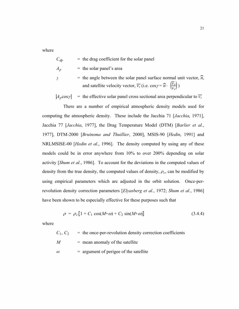
where
Cdp = the drag coefficient for the solar panel
Ap = the solar panel’s area
γ = the angle between the solar panel surface normal unit vector, n,
and satellite velocity vector, vr (i.e. cosγ = n ⋅ vrvr
)
Apcosγ = the effective solar panel cross sectional area perpendicular to vr
There are a number of empirical atmospheric density models used for
computing the atmospheric density. These include the Jacchia 71 [Jacchia, 1971],
Jacchia 77 [Jacchia, 1977], the Drag Temperature Model (DTM) [Barlier et al.,
1977], DTM-2000 [Bruinsma and Thuillier, 2000], MSIS-90 [Hedin, 1991] and
NRLMSISE-00 [Hedin et al., 1996]. The density computed by using any of these
models could be in error anywhere from 10% to over 200% depending on solar
activity [Shum et al., 1986]. To account for the deviations in the computed values of
density from the true density, the computed values of density, ρc, can be modified by
using empirical parameters which are adjusted in the orbit solution. Once-per-
revolution density correction parameters [Elyasberg et al., 1972; Shum et al., 1986]
have been shown to be especially effective for these purposes such that
ρ = ρc 1 + C1 cos(M+ω) + C2 sin(M+ω) (3.4.4)
where
C1, C2 = the once-per-revolution density correction coefficients
M = mean anomaly of the satellite
ω = argument of perigee of the satellite

22
3.4.2 Solar Radiation Pressure
The Sun emits a nearly constant amount of photons per unit of time. At a
mean distance of 1 A.U. from the Sun, this radiation pressure is characterized as a
momentum flux having an average value of 4.56×10⁻⁶ N /m 2. The direct solar
radiation pressure from the Sun on a satellite is modeled as [Tapley and Ries, 1987]
Psolar = - P (1 + η) Am ν u (3.4.5)
where
P = the momentum flux due to the Sun
η = reflectivity coefficient of the satellite
A = the cross-sectional area of the satellite normal to the Sun
m = mass of the satellite
ν = the eclipse factor (ν = 0 if the satellite is in full shadow, ν = 1 if
the satellite is in full Sun, and 0 < ν < 1 if the satellite is in
partial shadow)
u = the unit vector pointing from the satellite to the Sun
Similarly, the solar radiation pressure perturbation on an individual satellite surface,
like the satellite’s solar panel, can be modeled as
Ppanels = - P ν Apcosγ
m u + ηp n (3.4.6)
where
Ap = the solar panel area
n = the surface normal unit vector of the solar panel

23
γ = the angle between the solar panel surface normal unit vector, n,
and satellite-Sun unit vector, u (i.e. cos γ = u ⋅ n )
Apcosγ = the effective solar panel cross sectional area perpendicular to u
The reflectivity coefficient, η, represents the averaged effect over the whole satellite
rather than the actual surface reflectivity. Conical or cylindrical shadow models for
the Earth and the lunar shadow are used to determine the eclipse factor, ν. Since
there are discontinuities in the solar radiation perturbation across the shadow
boundary, numerical integration errors occur for satellites, which are in the
shadowing region. The modified back differences (MBD) method [Anderle, 1973]
can be implemented to account for these errors [Lundberg, 1985; Feulner, 1990].
3.4.3 Earth Radiation Pressure
Not only the direct solar radiation pressure, but also the radiation pressure
imparted by the energy flux of the Earth should be modeled for the precise orbit
determination of any near-Earth satellite. The Earth radiation pressure model can be
summarized as follows [Knocke and Ries, 1987; Knocke, 1989].
( )1
ˆ(1 ) ' cosN
cearth e s s B
j j
AP A aE eM rmc
η τ θ=
= + + ∑ (3.4.7)
where
ηe = satellite reflectivity for the Earth radiation pressure
A ' = the projected, attenuated area of a surface element of the Earth
Ac = the cross sectional area of the satellite
m = the mass of the satellite
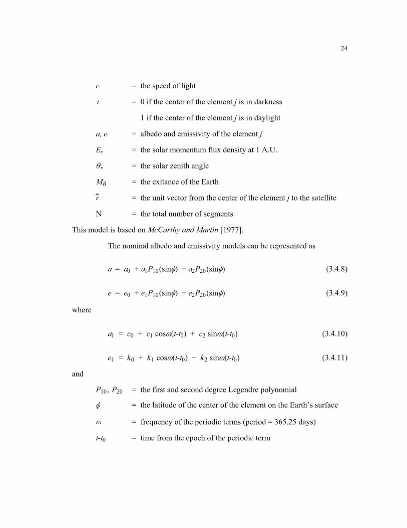
24
c = the speed of light
τ = 0 if the center of the element j is in darkness
1 if the center of the element j is in daylight
a, e = albedo and emissivity of the element j
Es = the solar momentum flux density at 1 A.U.
θs = the solar zenith angle
MB = the exitance of the Earth
r = the unit vector from the center of the element j to the satellite
N = the total number of segments
This model is based on McCarthy and Martin [1977].
The nominal albedo and emissivity models can be represented as
a = a0 + a1P10(sinφ) + a2P20(sinφ) (3.4.8)
e = e0 + e1P10(sinφ) + e2P20(sinφ) (3.4.9)
where
a1 = c0 + c1 cosω(t-t0) + c2 sinω(t-t0) (3.4.10)
e1 = k0 + k1 cosω(t-t0) + k2 sinω(t-t0) (3.4.11)
and
P10, P20 = the first and second degree Legendre polynomial
φ = the latitude of the center of the element on the Earth’s surface
ω = frequency of the periodic terms (period = 365.25 days)
t-t0 = time from the epoch of the periodic term

25
This model, based on analyses of Earth radiation budgets by Stephens et al. [1981],
characterizes both the latitudinal variation in Earth radiation and the seasonally
dependent latitudinal asymmetry.
3.4.4 Thermal Radiation Perturbation
Since the temperatures of the satellite’s surface are not uniform due to the
internal and external heat fluxes, there exists a force due to a net thermal radiation
imbalance. This perturbation depends on the shape, the thermal property, the pattern
of thermal dumping, the orbit characteristics, and the thermal environment of the
satellite as a whole. This modeling can be quite complex. For example, if a satellite
has active louvers for heat dissipation, the thermal force can have specular
characteristics whereas the heat loss to space from a flat plat is normally diffusive.
Even a clean, perfect spherical satellite like Lageos [Ries, 1989] has been found to
have a range of detectable thermally induced forces. It is observed for GPS satellites
that there are unexplained forces in the body-fixed +Y or -Y direction, that is along
solar panel rotation axis, which causes unmodeled accelerations [Fliegel et al., 1992]
believed to be of thermal origin. This acceleration is referred to as the “Y-bias”.
Possible causes of the Y-bias are solar panel axis misalignment, solar sensor
misalignment, and the heat generated in the GPS satellite body, which is radiated
preferentially from louvers on the +Y side. Since this Y-bias perturbation is not
predictable, it can be modeled as
Pybias = α ⋅ uY (3.4.12)

26
where uY is a unit vector in the Y-direction, and the scale factor, α, is estimated for
each GPS satellite. Models, which are satellite-specific, are required to properly
account for these effects depending on the orbit accuracy needed within a given
application.
3.4.5 GPS Solar Radiation Pressure Models
At the 20,000-km altitude of GPS satellite, solar radiation is the dominant
non-gravitational force acting on the spacecraft. Several GPS solar radiation pressure
models are currently available, and two of those models are summarized in this
section.
Rockwell International Corporation, which was the spacecraft contractor
for the Block I and II GPS satellites, developed GPS satellite solar radiation pressure
models, known as ROCK4 for Block I, and ROCK42 for Block II [Fliegel et al.,
1992]. These models treat a spacecraft as a set of flat or cylindrical surfaces.
Diffusive and specular forces acting on each surface are computed and summed in the
spacecraft body-fixed coordinate system. The +Z direction is toward the satellite-
Earth vector. The +Y direction is along one of the solar panel center beams. The
satellite is maneuvered so that the X-axis will be kept in the plane defined by the
Earth, the Sun and the satellite. As a result, the solar radiation pressure forces are
confined in the X-Z plane, since the Y-axis is perpendicular to the Earth, Sun and the
satellite plane. The ROCK4 model also provides solar radiation formulas for the X-
and Z- acceleration components as a function of the angle between the Sun and the
+Z-axis, e.g. T10 for Block I, and T20 for Block II GPS satellites [Fliegel et al.,
1992].
27
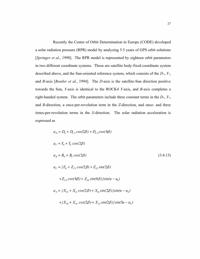
Recently the Center of Orbit Determination in Europe (CODE) developed
a solar radiation pressure (RPR) model by analyzing 5.5 years of GPS orbit solutions
[Springer et al., 1998]. The RPR model is represented by eighteen orbit parameters
in two different coordinate systems. Those are satellite body-fixed coordinate system
described above, and the Sun-oriented reference system, which consists of the D-, Y-,
and B-axis [Beutler et al., 1994]. The D-axis is the satellite-Sun direction positive
towards the Sun, Y-axis is identical to the ROCK4 Y-axis, and B-axis completes a
right-handed system. The orbit parameters include three constant terms in the D-, Y-,
and B-direction, a once-per-revolution term in the Z-direction, and once- and three
times-per-revolution terms in the X-direction. The solar radiation acceleration is
expressed as
aD = D0 + DC 2 cos(2β ) + DC 4 cos(4β )
aY = Y0 + YC cos(2β )
aB = B0 + BC cos(2β ) (3.4.13)
aZ = Z0 + ZC2 cos(2β) + ZS2 sin(2β )
+ZC4 cos(4β ) + ZS4 sin(4β )sin(u − u0 )
aX = X10 + X1C cos(2β ) + X1S sin(2β )sin(u − u0 )
+X30 + X3C cos(2β ) + X3S sin(2β )sin(3u − u0 )

28
where u is the argument of latitude of satellite in the orbit plane, u0 is the latitude of
the Sun in the orbit plane, and β is the angular distance between the orbit plane and
the Sun.
3.4.6 ICESat/GLAS "Box-Wing" Model
For modeling of non-gravitational perturbations on T/P, the "box-wing"
model or the so-called macro-model [Marshall et al., 1992] was developed based on a
thermal analysis of the spacecraft [Antreasian and Rosborough, 1992]. In the macro-
model, the spacecraft main body and the solar panel are represented by a simple
geometric model, a box and a wing, and the solar radiation and the thermal forces are
computed for each surface and summed over the surfaces. For example, the solar
radiation acceleration for the macro-model is computed using the following equation
[Milani et al., 1987].
1
ˆ ˆcos 2( cos ) (1 )3
nfacei
solar i i i i i ii
P P A n sm
α ν δθ ρ θ ρ=
⋅ = − + + − ∑ (3.4.14)
where
Psolar = the solar radiation pressure acceleration
P = the momentum flux due to the Sun
α = the scale factor of the acceleration
ν = the eclipse factor (0 for full shadow, 1 for full Sun)
m = mass of the satellite
Ai = surface area of the i-th plate
θ i = angle between surface normal and satellite-Sun vector for i-th
plate

29
ni = surface normal unit vector for i-th plate
s = satellite-Sun unit vector
δi = specular reflectivity for i-th plate
ρi = diffusive reflectivity for i-th plate
nface = total number of plates in the model
A similar model is being developed for the ICESat/GLAS satellite, and the model
parameters, including the specular and diffusive reflectivity coefficients, will be
tuned using the tracking data.
3.5 Empirical Forces
To account for the unmodeled forces, which act on the satellite or for
incorrect force models, some empirical parameters are customarily introduced in the
orbit solution. These include the empirical tangential perturbation and the one-cycle-
per-orbital-revolution (1cpr) force in the radial, transverse, and normal directions
[Colombo, 1986; Colombo, 1989]. Especially for satellites like ICESat/GLAS which
are tracked continuously with high precision data, introduction of these parameters
can significantly reduce orbit errors occurring at the 1cpr frequency and in the along
track direction [Rim et al., 1996].
3.5.1 Empirical Tangential Perturbation
Unmodeled forces in the tangential direction, either along the inertial
velocity or along the body-fixed velocity, may be estimated by using empirical

30
models during the orbit determination process. This tangential perturbation can be
modeled empirically as
Ptangen = Ct ut (3.5.1)
where
Ct = empirical tangential parameter
ut = the unit vector in the tangential direction (along inertial velocity
or body-fixed velocity)
Such forces are estimated when it is believed that there are mismodeled or unmodeled
non-conservative forces in the tangential direction. A set of piecewise constants, Ct,
can be estimated to account for these unmodeled tangential perturbations.
3.5.2 Once-per Revolution RTN Perturbation
Unmodeled perturbations in the radial, transverse, and normal directions
can be modeled as
Prtn = PrPtPn
= Cr cosu + Sr sinuCt cosu + St sinuCn cosu + Sn sinu
(3.5.2)
where
Pr = one-cycle-per-revolution radial perturbation
Pt = one-cycle-per-revolution transverse perturbation
Pn = one-cycle-per-revolution normal perturbation
u = the argument of latitude of the satellite
Cr, Sr = the one-cycle-per-revolution radial parameters

31
Ct, St = the one-cycle-per-revolution transverse parameters
Cn, Sn = the one-cycle-per-revolution normal parameters
These empirical perturbations, which are computed in the radial, transverse, and
normal components, are transformed into the geocentric inertial components. These
parameters are introduced as needed with complete or subsets of empirical terms
being used.

32
4.0 ALGORITHM DESCRIPTION: Measurements
4.1 ICESat/GLAS Measurements Overview
The GPS measurements will be the primary measurement type for the
ICESat/GLAS POD, while the laser range measurement will serve as a secondary
source of verification and evaluation of the GPS-based ICESat/GLAS POD product.
In this chapter, the mathematical models of the GPS and laser range measurements
are discussed.
4.2 GPS Measurement Model
The GPS measurements are ranges, which are computed from measured
time or phase differences between received signals and receiver generated signals.
Since these ranges are biased by satellite and receiver clock errors, they are called
pseudoranges. In this section, code pseudorange (PR) measurements, phase
pseudorange measurements (PPR), double-differenced high-low phase pseudorange
measurements (DDHL) which involve one ground station, two GPS satellites, and
one low Earth orbiting satellite, are discussed. Consult Hofmann-Wellenhof et al.
[1992] and Remondi [1984] for more discussion of GPS measurement models.
4.2.1 Code Pseudorange Measurement
The PR measurement, ρ cPR , can be modeled as follows,
ρ cPR = ρ - c ⋅ δtt + c ⋅ δtr + δρtrop + δρiono + δρrel (4.2.1)

33
where ρ is the slant range between the GPS satellite and the receiver receiving the
GPS signal, c is the speed of light, δtt is the GPS satellite's clock error, δtr is the
receiver's clock error, δρtrop is the tropospheric path delay, δρiono is the ionospheric
path delay, and δρrel is the correction for relativistic effects.
4.2.2 Phase Pseudorange Measurement
The carrier phase measurement between a GPS satellite and a ground
station can be modeled as follows,
φ cij(tRi) = φ j(tTi) - φi(tRi) + Ni
j(t0 i) (4.2.2a)
where tRi is the receive time at the i-th ground receiver, tTi is the transmit time of the j-
th satellite’s phase being received by the i-th receiver at tRi, φcij(tRi) is the computed
phase difference between the j-th GPS satellite and i-th ground receiver at tRi, φj(tTi) is
the phase of j-th GPS satellite signal received by i-th receiver, φi(tRi) is the phase of i-
th ground receiver at tRi, t0i is the initial epoch of the i-th receiver, and Nij(t0i) is the
integer bias which is unknown and is often referred to as an "ambiguity bias".
Similarly, the carrier phase measurement between a GPS satellite and a low satellite
can be modeled as follows,
φ cuj(tRu) = φ j(tTu) - φu(tRu) + Nu
j(t0u) (4.2.2b)
where tRu is the received time of the on-board receiver of the user satellite, tTu is the
transmit time of the j-th satellite’s phase being received by the user satellite at tRu,
φ cuj(tRu) is the computed phase difference between j-th GPS satellite and the user
satellite at tRu, φ j(tTu) is the phase of j-th GPS satellite signal received by the user

34
satellite, φu(tRu) is the phase of the user satellite at tRu, t0u is the initial epoch of the
user satellite, and Nuj(t0u) is the unknown integer bias.
The signal transmit time of the j-th GPS satellite can be related to the
signal receive time by
tTij = tRi - (ρi
j(tRi)/c) - δtφij (4.2.3a)
tTuj = tRu - (ρu
j(tRu)/c) - δtφuj (4.2.3b)
where ρij is the geometric line of sight range between j-th GPS satellite and i-th
ground receiver, ρuj is the slant range between j-th GPS satellite and the on-board
receiver of the user satellite, δtφij is the sum of ionospheric delay, tropospheric delay,
and relativistic effect on the signal traveling from j-th GPS satellite to i-th ground
receiver, δtφuj is the sum of ionospheric path delay, tropospheric path delay, and
relativistic effect on the signal traveling from j-th satellite to the on-board receiver of
the user satellite. Since the time tag, ti or tu, of the measurement is in the receiver
time scale which has some clock error, the true receive times are
tRi = ti - δtci (4.2.4a)
tRu = tu - δtcu (4.2.4b)
where δtci is the clock error of the i-th ground receiver at tRi and δtcu is the clock error
of the on-board receiver of the user satellite at tRu. Since the satellite oscillators and
the receiver oscillators are highly stable clocks, the (1σ) change of the frequency over
the specified period, ∆ff
, is on the order of 10-12. With such high stability, the linear
approximation of φ (t + δt ) = φ (t) + f ⋅ δt can be used for δt which is usually

35
less than 1 second. By substituting Eqs. (4.2.3a) and (4.2.4a) into Eq. (4.2.2a), and
neglecting higher order terms, Eq. (4.2.2a) becomes
φ cij(tRi) = φ j(ti) - f j⋅ [ δtci + ρi
j(tRi)/c + δtφi
j ]
- φi(ti) + fi δtci + Nij(t0i) (4.2.5a)
Similarly, the phase measurement between the j-th GPS satellite and the user satellite
can be modeled as follows,
φ cuj(tRu) = φ j(tu) - f j⋅ [ δtcu + ρu
j(tRu)/c + δtφu
j ]
- φu(tu) + fu δtcu + Nuj(t0u) (4.2.5b)
By multiplying a negative nominal wavelength, -λ = -c / f0, where f0 is the
nominal value for both the transmit frequency of the GPS signal and the receiver
mixing frequency, Eq. (4.2.5a) becomes the phase pseudorange measurement,
PPRcij = f
j
f0 ρi
j(tRi) + fj
f0 δρφi
j + fj
f0 c δtci -
fif0
c δtci
- cf0
⋅ φ j(ti) - φi(ti) + Cij (4.2.6)
where δρφi
j = c δtφi
j and Cij = - c
f0 ⋅ Ni
j.
The first term of second line of Eq. (4.2.6) can be expanded using the following
relations:
φ j(ti) - φi(ti) = φ j(t0) - φi(t0) + f j - fi dtt0
ti
(4.2.7)
However, φ j(t0) - φi(t0) = f j δtcj(t0) - fi δtci(t0), which is the time difference
between the satellite and the receiver clocks at the first data epoch, t0. And

36
f j - fi dtt0
ti
is the total number of cycles the two oscillators have drifted apart over
the interval from t0 to ti. According to Remondi [1984], this is equivalent to the
statement that the two clocks have drifted apart, timewise, by amount
δtcj(ti) - δtci(ti) - δtc
j(t0) - δtci(t0) . Thus,
φ j(ti) - φi(ti) = f j ⋅ δtcj - fi ⋅ δtci (4.2.8)
After substituting Eq. (4.2.8), Eq. (4.2.6) becomes,
PPRcij = f
j
f0 ρi
j(tRi) + fj
f0 δρφi
j - fj
f0 c δtc
j + fj
f0 c δtci + Ci
j (4.2.9a)
Similarly, the phase pseudorange between j-th satellite and a user satellite can be
written as,
PPRcuj = f
j
f0 ρu
j(tRu) + fj
f0 δρφu
j - fj
f0 c δtc
j + fj
f0 c δtcu + Cu
j (4.2.9b)
Since the GPS satellites have highly stable oscillators, which have 10-11 or 10-12
clock drift rate, the frequencies of those clocks usually stay close to the nominal
frequency, f0. If the frequencies are expressed as f j = f0 + ∆f j, where ∆f is clock
frequency offset from the nominal value, Eqs. (4.2.9a) and (4.2.9b) become as
follows after ignoring negligible terms:
PPRcij = ρi
j(tRi) + δρφi
j - c δtcj + c δtci + Ci
j (4.2.10a)
PPRcuj = ρu
j(tRu) + δρφu
j - c δtcj + c δtcu + Cu
j (4.2.10b)
Note that ρij(tRi) and ρu
j(tRu) could be expanded as
ρij(tRi) = ρi
j(ti) - ρij δtci (4.2.11a)
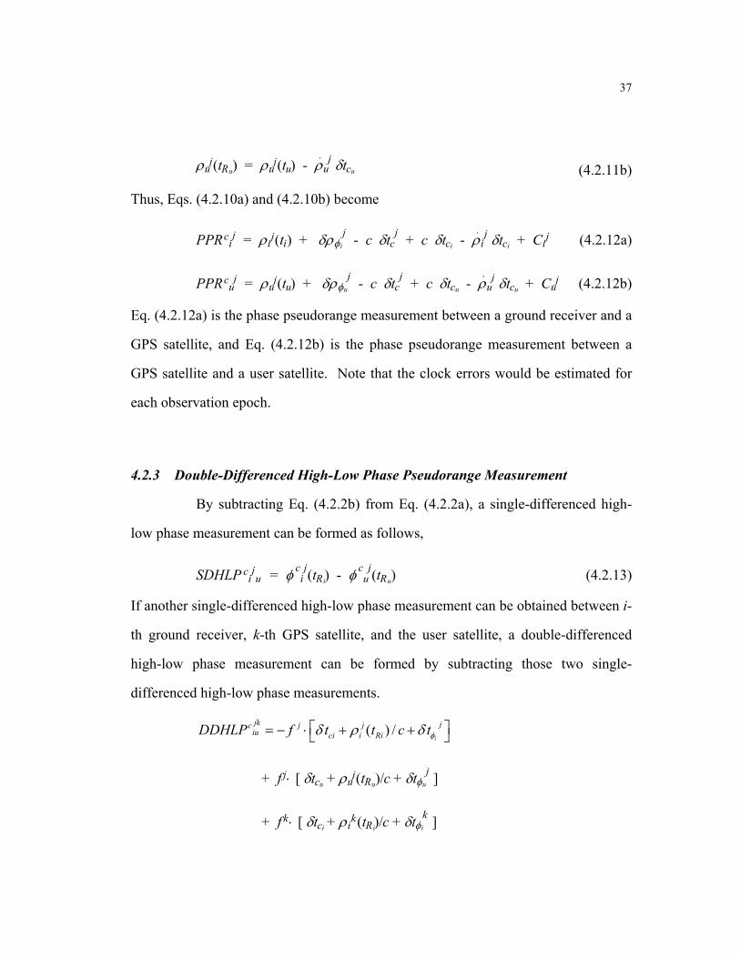
37
ρuj(tRu) = ρu
j(tu) - ρuj δtcu (4.2.11b)
Thus, Eqs. (4.2.10a) and (4.2.10b) become
PPRcij = ρi
j(ti) + δρφi
j - c δtcj + c δtci - ρi
j δtci + Cij (4.2.12a)
PPRcuj = ρu
j(tu) + δρφu
j - c δtcj + c δtcu - ρu
j δtcu + Cuj (4.2.12b)
Eq. (4.2.12a) is the phase pseudorange measurement between a ground receiver and a
GPS satellite, and Eq. (4.2.12b) is the phase pseudorange measurement between a
GPS satellite and a user satellite. Note that the clock errors would be estimated for
each observation epoch.
4.2.3 Double-Differenced High-Low Phase Pseudorange Measurement
By subtracting Eq. (4.2.2b) from Eq. (4.2.2a), a single-differenced high-
low phase measurement can be formed as follows,
SDHLP ciju = φ c
ij(tRi) - φ
cuj(tRu) (4.2.13)
If another single-differenced high-low phase measurement can be obtained between i-
th ground receiver, k-th GPS satellite, and the user satellite, a double-differenced
high-low phase measurement can be formed by subtracting those two single-
differenced high-low phase measurements.
( ) /i
jk jc j jiu ci i RiDDHLP f t t c tφδ ρ δ = − ⋅ + +
+ f j⋅ [ δtcu + ρuj(tRu)/c + δtφu
j ]
+ f k ⋅ [ δtci + ρik(tRi)/c + δtφi
k ]

38
- f k ⋅ [ δtcu + ρuk(tRu)/c + δtφu
k ]
+ φ j(ti) - φk(ti) - φ
j(tu) + φ k(tu)
jkiuN+ (4.2.14)
where 0 0 0 0( ) ( ) ( ) ( )jk j j k kiu i i u u i i u uN N t N t N t N t= − − + . In Eq. (4.2.14), all the phase
terms associated with the ground station and user satellite receivers are canceled out.
By multiplying a negative nominal wave length, -λ = -c / f0, Eq. (4.2.14)
becomes the double-differenced high-low phase pseudorange measurement,
( ) ( )0 0
( ) ( ) ( ) ( )i u i u
j kjkc j j k kiu i R u R i R u R
f fDDHL t t t tf f
ρ ρ ρ ρ
= ⋅ − − ⋅ −
( )0
( ) ( ) ( ) ( )j k j ki i u u
c t t t tf
φ φ φ φ
− ⋅ − − +
+ c ⋅ f j - f k
f0⋅ (δtci - δtcu)
+ f j
f0 ⋅ (δρφi
j - δρφu
j) - f k
f0 ⋅ (δρφi
k - δρφu
k)
jkiuC+ (4.2.15)
where δρφ = -c ⋅ δtφ, and jk jkiu iuC Nλ= − ⋅ . Note that Eq. (4.2.15) contains two
different time tags, ti and tu. If the ground station receiver clock and the on-board
receiver clock are synchronized, then the second line can be canceled out. Since both
the ICESat/GLAS on-board receiver clock and the ground station receiver clock will

39
be synchronized within 1 microsecond with the GPS System Time, the second line
can be canceled out.
Since the GPS satellites have highly stable oscillators, which have 10-11 or
10-12 clock drift rate, the frequencies of those clocks usually stay close to the nominal
frequency, f0. If the frequencies are expressed as f j = f0 + ∆f j and f k = f0 + ∆f k ,
Eq. (4.2.15) becomes
DDHLc
iujk
= ρij (tRi
) − ρuj(tRu
) − ρik (tRi
) + ρuk (tRu
)
+ ∆f j
f0⋅ (ρi
j(tRi) - ρuj(tRu)) - ∆f k
f0⋅ (ρi
k(tRi) - ρuk(tRu))
+ c ⋅ ∆f j - ∆f k
f0⋅ (δtci - δtcu)
+ δρφi
j - δρφu
j - δρφi
k + δρφu
k
+ ∆f j
f0 ⋅ (δρφi
j - δρφu
j) - ∆f k
f0 ⋅ (δρφi
k - δρφu
k)
jkiuC+ (4.2.16)
For the ICESat/GLAS-GPS case, the single differenced range can be 600 km to 6200
km. If we assume 10-11 clock drift rate for GPS satellite clocks, the second line
contributes an effect, which is at the sub-millimeter level to the double differenced
range measurement. This effect is less than the noise level, and as a consequence, the
contribution from the second line can be ignored. Since the performance
specification of the time-tag errors of the flight and ground receivers for
ICESat/GLAS mission is required to be less than 1 microsecond with respect to the

40
GPS System Time, the third line also is negligible. The fifth line is totally negligible,
because even for the propagation delay of 100 m, the contribution from this line is
less than 10-9 meters. The first line in Eq. (4.2.16) can be expanded by the linear
approximation after substituting Eqs. (4.2.4a) and (4.2.4b), to obtain:
DDHLc
iujk
= ρij (ti) − ρu
j( tu ) − ρik (ti ) + ρu
k(tu )
- ρij(ti) - ρi
k(ti) ⋅ δtci + ρuj(tu) - ρu
k(tu) ⋅ δtcu
+ δρφi
j - δρφu
j - δρφi
k + δρφu
k
jkiuC+ (4.2.17)
This equation is implemented for the double-differenced high-low phase pseudorange
measurement. The second line does not need to be computed if the ground stations
and the ICESat/GLAS on-board receiver’s time-tags are corrected in the
preprocessing stage by using independent clock information from the pseudo-range
measurement. If such clock information is not available, then the receiver clock
errors, δtci and δtcu, can be modeled as linear functions,
δtci = ai + bi (ti - ti0) (4.2.18a)
δtcu = au + bu (tu - tu0) (4.2.18b)
where (ai, bi) and (au, bu) are pairs of clock bias and clock drift for i-th ground station
receiver clock and the user satellite clock, respectively, and ti0 and tu0 are the
reference time for clock parameters for i-th ground station receiver clock and the user
satellite clock.

41
The third line of Eq. (4.2.17) includes the propagation delay and the
relativistic effects for the high-low phase converted measurement. These effects are
discussed in more detail in the following sections.
4.2.4 Corrections
4.2.4.1 Propagation Delay
When a radio wave is traveling through the atmosphere of the Earth, it
experiences a delay due to the propagation refraction. Atmospheric scientists usually
divide the atmosphere into four layers: the troposphere, the stratosphere, the
mesosphere, and the thermosphere. The troposphere, the lowest layer of the Earth’s
atmosphere, contains 99% of the atmosphere’s water vapor and 90% of the air mass.
The tropospheric bending is therefore treated using both dry and wet components.
The dry path delay is caused by the atmosphere gas content along the propagated path
through the troposphere while the wet path delay is caused by the water vapor content
along the same path. Since the tropospheric path delay of a radio wave is frequency
independent, this path delay cannot be isolated using multiple frequencies. The
tropospheric path delays caused by the dry portion, which accounts for 80% or more
of the delay, can be modeled with an accuracy of two to five percent for L-band
frequencies [Atlshuler & Kalaghan, 1974]. Although the contribution from the wet
component is relatively small, it is more difficult to model because surface
measurements of water vapor cannot be applied to completely describe the regional
variations in the water vapor distribution, especially with respect to horizontal

42
variation, of the water vapor field. There are several approaches to model the wet
component of the tropospheric path delay. One approach is to use one of the
empirical atmospheric models based on the measurement of meteorological
parameters at the Earth’s surface or the altitude profile with radisondes and apply
regional modeling. The other approach is to map the water vapor content in various
directions directly using devices like water vapor radiometer (WVR). List of
references for these approaches can be found in Tralli et al. [1988]. A third approach
is to solve for tropospheric path delay parameters. Chao’s model [Chao, 1974],
modified Hopfield model [Goad and Goodman, 1974; Remondi, 1984], or MTT
model [Herring, 1992] are among several candidates which can be implemented for
the tropospheric correction.
The ionosphere is a region of the Earth’s upper atmosphere, approximately
100 km to 1000 km above the Earth’s surface, where electrons and ions are present in
quantities sufficient to affect the propagation of radio waves. The path delay will be
proportional to the number of electrons along the slant path between the satellite and
the receiver, and the electron density distribution varies with altitude, time of day
time of year, solar and geomagnetic activity, and the time within the solar sunspot
cycle. The ionospheric path delay depends on the frequency of the radio signal. The
ionospheric bending on L1 GPS measurement will vary from about 0.15 m to 50 m
[Clynch and Coco, 1986]. Some of this delay can be eliminated by ionospheric
modeling [for example, Finn and Matthewman, 1989]. However, more accurate
corrections can be made by using the dual frequency measurements routinely
acquired by the GPS receivers. The correction method for the dual frequency GPS

43
measurements can be found in Section 6.5.2. Hofmann-Wellenhof et al. [1992]
provides more detailed description of the propagation delay for GPS measurements.
4.2.4.2 Relativistic Effect
The relativistic effects on GPS measurements can be summarized as
follows. Due to the difference in the gravitational potential, the satellite clock tends
to run faster than the ground station’s [Spilker, 1978; Gibson, 1983]. These effects
can be divided into two parts: a constant drift and a periodic effect. The constant drift
can be removed by off-setting the GPS clock frequency low before launch to account
for that constant drift. The periodic relativistic effects can be modeled for a high-low
measurement as
∆ρ srel = 2c (rl ⋅ vl - rh ⋅ vh) (4.2.20)
where
∆ρ srel = correction for the special relativity
c = speed of light
rl, vl = the position and velocity of the low satellite or tracking stations
rh, vh = the position and velocity of the high satellite
The coordinate speed of light is reduced when light passes near a massive body
causing a time delay, which can be modeled as [Holdridge, 1967]
∆ρgrel = (1 + γ) GMec2
ln rtr + rrec + ρrtr + rrec - ρ
(4.2.21)
where
∆ρgrel = correction for the general relativity
44
γ = the parameterized post-Newtonian (PPN) parameter (γ = 1 for
general relativity)
GMe = gravitational constant for the Earth
ρ = the relativistically uncorrected range between the transmitter
and the receiver
rtr = the geocentric radial distance of the transmitter
rrec = the geocentric radial distance of the receiver
4.2.4.3 Phase Center Offset
The geometric offset between the transmitter and receiver phase centers
and the effective satellite body-fixed reference point can be modeled depending on
the satellite orientation (attitude) and spacecraft geometry. The ICESat/GLAS
antenna location will be known and implemented when the fabrication of the satellite
is complete. However, the location of the antenna phase center with respect to the
spacecraft center of mass will also be required. This position vector will be
essentially constant in spacecraft fixed axes, but this correction is necessary since the
equations of motion refer to the spacecraft center of mass.
4.2.4.4 Ground Station Related Effects
In computing the double-differenced phase-converted high-low pseudo-
range measurement, it is necessary to consider the effects of the displacement of the
ground station location caused by the crustral motions. Among these effects, tidal
effects and tectonic plate motion effects are most prominent.

45
Station displacements arising from tidal effects can be divided into three
parts,
∆tide = ∆dtide + ∆ocean + ∆rotate (4.2.22)
where
∆tide = the total displacement due to the tidal effects
∆dtide = the displacement due to the solid Earth tide
∆ocean = the displacement due to the ocean loading
∆rotate = the displacement due to the rotational deformation
The approach of the IERS Conventions [McCarthy, 1996] have been implemented for
the solid Earth tide correction. Ocean loading effects are due to the elastic response
of the Earth’s crust to loading induced by the ocean tides. The displacement due to
the rotational deformation is the displacement of the ground station by the elastic
response of the Earth’s crust to shifts in the spin axis orientation [Goad, 1980] which
occur at both tidal and non-tidal periods. Detailed models for the effects of solid
Earth tide, the ocean loading, and the rotational deformation, can be found in Yuan
[1991].
The effect of the tectonic plate motion, which is based on the relative plate
motion model AM0-2 of Minster and Jordan [1978], is modeled as
∆ tect = (ω p × R s0)(ti − t0 ) (4.2.23)
where
∆ tect = the displacement due to the tectonic motion
ωp = the angular velocity of the tectonic plate
Rs0 = the Earth-fixed coordinates of the station at ti

46
t0 = a reference epoch
4.2.5 Measurement Model Partial Derivatives
The partial derivatives of Eq. (4.2.18) with respect to various model
parameters are given in this section. The considered parameters include the ground
station positions, GPS satellite’s positions, ICESat's positions, clock parameters,
ambiguity parameters, and tropospheric refraction parameters.
The partial derivatives of Eq. (4.2.18) with respect to the i-th ground
station positions, (x1i, x2i, x3i), are
( ) ( )jk j kciu mi m mi m
j kmi i i
DDHL x x x xx ρ ρ
∂ − −= −
∂, for m=1,2,3 (4.2.24)
where ρij is the range between i-th ground station receiver and j-th transmitter, and
ρik is the range between i-th ground station receiver and k-th transmitter such that
ρij = (x1i - x1j)2 + (x2i - x2j)2 + (x3i - x3j)2 (4.2.25)
ρik = (x1i - x1k)2 + (x2i - x2k)2 + (x3i - x3k)2 (4.2.26)
and (x1j, x2j, x3j) and (x1k , x2k , x3k) are the j-th and k-th transmitter Cartesian
positions, respectively.
The partial derivatives of Eq. (4.2.18) with respect to the j-th and k-th
transmitter positions are

47
( ) ( )jk j jciu mi m mu m
j j ji um
DDHL x x x xx ρ ρ
∂ − −= +
∂, for m=1,2,3 (4.2.27)
( ) ( )jk k kciu mi m mu m
k k ki um
DDHL x x x xx ρ ρ
∂ − −= −
∂, for m=1,2,3 (4.2.28)
where ρuj is the range between j-th transmitter and the user satellite, and ρu
k is the
range between k-th transmitter and the user satellite such that
ρuj = (x1u - x1j)2 + (x2u - x2j)2 + (x3u - x3j)2 (4.2.29)
ρuk = (x1u - x1k)2 + (x2u - x2k)2 + (x3u - x3k)2 (4.2.30)
and (x1u, x2u, x3u) are the user satellite's Cartesian positions.
The partial derivatives of Eq. (4.2.18) with respect to the user satellite
positions are
( ) ( )jk j kciu mu m mu m
j kmu u u
DDHL x x x xx ρ ρ
∂ − −= − +
∂, for m=1,2,3 (4.2.31)
The partial derivatives of Eq. (4.2.18) with respect to the clock parameters
of Eqs. (4.2.19a) and (4.2.19b) are
( )jkciu j k
i ii
DDHLa
ρ ρ∂= − −
∂ (4.2.32)
0( ) ( )jkciu j k
i i i ii
DDHL t tb
ρ ρ∂= − − ⋅ −
∂ (4.2.33)
and

48
( )jkciu j k
u uu
DDHLa
ρ ρ∂= −
∂ (4.2.34)
0( ) ( )jkciu j k
u u u uu
DDHL t tb
ρ ρ∂= − ⋅ −
∂ (4.2.35)
The partial derivative of Eq. (4.2.18) for the double-differenced ambiguity
parameter, jkiuC , is
1jkciu
jkiu
DDHLC
∂=
∂ (4.2.36)
When Chao’s model is used, the partial derivative of Eq. (4.2.18) with
respect to the i-th ground station’s zenith delay parameter, Zi, is
1 10.00143 0.00035sin sin
tan 0.0445 tan 0.017
jkciu
j jii ij j
i i
DDHLZ E E
E E
∂ = +
∂ + + + +
1 10.00143 0.00035sin sin
tan 0.0445 tan 0.017k k
i ik ki i
E EE E
− + + + + +
(4.2.37)
where Eij and Ei
k are the elevation angles of the j-th and k-th GPS satellite
transmitters from i-th ground station, respectively.

49
4.3 SLR Measurement Model
4.3.1 Range Model and Corrections
Laser tracking instruments record the travel time of a short laser pulse
from the reference point (opticalaxis) to the satellite retroreflector and back. The
one-way range from the reference point of the ranging instrument to the retroreflector
of the satellite, ρ o, can be expressed in terms of the round trip light time, ∆τ as
ρ o = 12
c∆τ + ε (4.3.1)
where
c = the speed of light
ε = measurement error.
The computed one-way signal path between the reference point on the
satellite and the ground station, ρ c, can be expressed as
ρ c = r - rs + ∆ρ trop + ∆ρgrel + ∆ρc.m. (4.3.2)
where
r = the satellite position in geocentric coordinates
rs = the position of the tracking station in geocentric coordinates
∆ρ trop = correction for tropospheric delay
∆ρgrel = correction for the general relativity
∆ρc.m. = correction for the offset of the satellite's center-of-mass and the
laser retroreflector
The tropospheric refraction correction is computed using the model of Marini and
Murray [1973]. The correction for the general relativity in SLR measurements is the
50
same as for GPS measurement, which is expressed in Eq. (4.2.21). The effects of the
displacement of the ground station location caused by the crustral motions should be
considered. These crustral motions include tidal effects and tectonic plate motion
effects, which are described in Eqs. (4.2.22) and (4.2.23), respectively.
4.3.2 Measurement Model Partial Derivatives
The partial derivatives of Eq. (4.3.2) with respect to various model
parameters are derived in this section. The considered parameters include the ground
station positions, satellite’s positions.
The partial derivatives of Eq. (4.3.2) with respect to the ground station
positions, (rs1, rs2, rs3), are
( )csi i
si
r rrρ
ρ∂ −
=∂
, for i=1,2,3 (4.3.3)
where (r1, r2, r3) are the satellite's positions, and ρ is the range between the ground
station and the satellite such that
ρ = (r1 - rs1)2 + (r2 - rs2)2 + (r3 - rs3)2 (4.3.4)
The partial derivatives of Eq. (4.3.2) with respect to the satellite's
positions, (r1, r2, r3), are
( )ci si
i
r rrρ
ρ∂ −
=∂
, for i=1,2,3 (4.3.5)

51
5.0 ALGORITHM DESCRIPTION: Estimation
A least squares batch filter [Tapley, 1973] is our adopted approach for the
estimation procedure. Since multi-satellite orbit determination problems require
extensive usage of computer memory for computation, it is essential to consider the
computational efficiency in the problem formulation. This section describes the
estimation procedures for ICESat/GLAS POD, including the problem formulation for
multi-satellite orbit determination.
5.1 Least Squares Estimation
The equations of motion for the satellite can be expressed as
X (t) = F(X ,t), X (t0) = X 0 (5.1.1)
where X is the n-dimensional state vector, F is a non-linear n-dimensional vector
function of the state, and X 0 is the value of the state at the initial time t0, which is not
known perfectly. The tracking observations can be expressed as discrete
measurements of quantities, which are a function of the state. Thus the observation-
state relationship can be written as
Yi = G(X i, ti) + εi i = 1,… , l (5.1.2)
where Y i is a p vector of the observations made at time ti, (X i, ti) is a non-linear vector
function relating the state to the observations, and εi is the measurement noise.
If a reference trajectory is available and if X , the true trajectory, and X *,
the reference trajectory, remain sufficiently close throughout the time interval of
interest, the trajectory for the actual motion can be expanded in a Taylor series about
52
the reference trajectory to obtain a set of differential equations with time dependent
coefficients. Using a similar procedure to expand the nonlinear observation-state
relation, a linear relation between the observation deviation and the state deviation
can be obtained. Then, the nonlinear orbit determination problem can be replaced by
a linear orbit determination problem in which the deviation from the reference
trajectory is to be determined. In practice, this linearization of the problem requires
an iterative adjustment which yields successively smaller adjustments to the state
parameters to optimally fit the observations.
Let
x(t) = X (t) - X *(t) y(t) = Y (t) - Y *(t) (5.1.3)
where X*(t) is a specified reference trajectory and Y *(t) is the value of the observation
calculated by using X*(t). Then, substituting Eq. (5.1.3) into Eqs. (5.1.1) and (5.1.2),
expanding in a Taylor's series, and neglecting higher order terms leads to the relations
x = A(t)x, x(t0) = x0
yi = Hixi + εi i = 1,… ,l (5.1.4)
where
A(t) = ∂F
∂X(X *, t) H =
∂G
∂X(X*, t) (5.1.5)
The general solution to Eq. (5.1.4) can be expressed as
x(t) = Φ(t, t0)x0 (5.1.6)
where the state transition matrix Φ(t,t0) satisfies the differential equation:

53
Φ(t,t0) = A(t)Φ(t, t0), Φ(t0, t0) = I (5.1.7)
where I is the n ×n identity matrix.
Using Eq. (5.1.5), the second of Eq. (5.1.3) may be written in terms of the
state at t0 as
yi = HiΦ(ti,t0)x0 + εi, i = 1,… ,l (5.1.8)
Using the solution for the linearized state equation (Eq. (5.1.6)), Eq. (5.1.8) may be
rewritten as
y = Hx0 + ε (5.1.9)
where
1
l
yy
y
=
1 1 0
0
( , )
( , )l l
H t tH
H t t
Φ = Φ
1
l
εε
ε
=
(5.1.10)
where y and ε are m vectors (m = l×p) and H is an m×n matrix. Equation (5.1.9) is a
system of m equations in n unknowns. In practical orbit determination problems,
there are more observations than estimated parameters (m > n), which means that Eq.
(5.1.9) is overdetermined. It is usually assumed that the observation error vector, ε,
satisfies the a priori statistics, E[ε] = 0 and E[εεT] = W -1. By scaling each term in Eq.
(5.1.9) by W 1/2 , the condition
W 1/2 [εεT]W T/2 = W 1/2 W -1W T/2 = I (5.1.11)
is obtained.

54
An approach to obtain the best estimate of x, given the linear observation-
state relations (Eq. (5.1.9)) is described in the following discussions. The method
obtains the solution by applying successive orthogonal transformations to the linear
equations given in Eq. (5.1.9). Consider the quadratic performance index
J = 12
W 1/2 (Hx - y) 2 = 12
(Hx - y)TW(Hx - y) (5.1.12)
The solution to the weighted least-squares estimation problem (which is
equivalent to the minimum variance and the maximum likelihood estimation problem,
under certain restrictions) is obtained by finding the value x which minimizes Eq.
(5.1.12). To achieve the minimum value of Eq. (5.1.12) let Q be an m×m orthogonal
matrix. Hence, it follows that Eq. (5.1.12) can be expressed as
J = 12
QW 1/2 (Hx - y) 2 (5.1.13)
Now, if Q is selected such that
QW 1/2 H = R0
QW 1/2 y = be
(5.1.14)
where R is n×n upper-triangular, 0 is an (m-n)×n null matrix, b is n×1 vector, and e is
an (m-n)×1 vector. Equation (5.1.13) can be written then as
J(x) = 12
Rx - b 2 + 12
e 2 (5.1.15)
The value of x, which minimizes Eq. (5.1.12), is obtained by the solution
Rx = b (5.1.16)
and the minimum value of the performance index becomes
J(x) = 12
e 2 = 12
y - Hx 2 (5.1.17)
That is, e provides an estimate of the residual error vector.

55
The procedures are direct and for implementation requires only that a
convenient computational procedure for computing QW 1/2 H and QW 1/2 y be
available. The two most frequently applied methods are the Givens method, based on
a sequence of orthogonal rotations, and the Householder method, based on a series of
orthogonal reflections [Lawson and Hanson, 1974].
In addition to the expression for computing the estimate, the statistical
properties of the error in the estimate, R, are required. If the error in the estimate, η,
is defined as
η = x - x (5.1.18)
it follows that
E[η] = E[ ˆ x − x] = E[R−1b − x] (5.1.19)
Since
QW 1/2 y = QW 1/2 Hx + QW 1/2 ε
leads to
b = Rx + ε (5.1.20)
it follows that
E[η] = E[R−1(Rx + ˜ ε ) − x] = E[R−1 ˜ ε ] (5.1.21)
As noted in Eq. (5.1.11), if the observation error, ε, is unbiased, ε = QW 1/2 ε will be
unbiased and
E[η] = 0 (5.1.22)
56
Hence, x will be an unbiased estimate of x. Similarly, the covariance matrix for the
error in x can be expressed as
P = E[ηηT ]
= E[R -1εε TR -T] = R -1E[εε T]R -T (5.1.23)
If the observation error, ε, has a statistical covariance defined as E[εεT] = W -1, the
estimation error covariance matrix is given by
E[εε T] = W 1/2 E[εεT]W T/2 = W 1/2 W -1W T/2 = I. Consequently, relation (5.1.23) leads
to
P = R -1R -T (5.1.24)
It follows then that the estimate of the state and the associated error covariance matrix
are given by the expressions
x = R -1b (5.1.25)
P = R -1R -T (5.1.26)
5.2 Problem Formulation for Multi-Satellite Orbit Determination
Proper categorization of the parameters will help to clarify the problem
formulation. Parameters can be divided into two groups: dynamic parameters and
kinematic parameters. Dynamic parameters need to be mapped into other states by
using the state transition matrix, which is usually computed by numerical integration,
while kinematic parameters are treated as constant throughout the computation.
Dynamic parameters can be grouped again into two parts as the local dynamic

57
parameters and global dynamic parameters. Local dynamic parameters are satellite-
specific. Global dynamic parameters are parameters, which influence every satellite,
such as those defining gravitational forces.
Following the categorization described above, the estimation state vector
is defined as
X ≡
X KPX SS
X LDPX GDP
(5.2.1)
where
X KP = the kinematic parameters (nkp )
X SS = the satellite states (nss)
X LDP = the local dynamic parameters (nldp)
X GDP = the global dynamic parameters (ngdp)
and X SS consists of satellites’ positions and velocities, i.e. X SS ≡ X POS, X VELT. For
ns-satellites, where ns is the total number of satellites which will be estimated, X SS
becomes
1
1
ns
ss
ns
r
rX
v
v
=
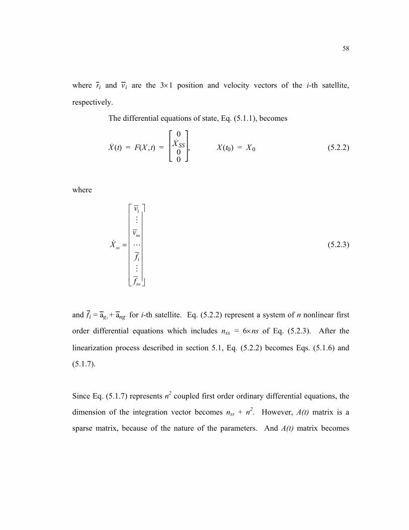
58
where ri and vi are the 3×1 position and velocity vectors of the i-th satellite,
respectively.
The differential equations of state, Eq. (5.1.1), becomes
X (t) = F(X , t) =
0X SS
00
, X (t0) = X 0 (5.2.2)
where
1
1
ns
ss
ns
v
vX
f
f
=
(5.2.3)
and fi = agi + ang i for i-th satellite. Eq. (5.2.2) represent a system of n nonlinear first
order differential equations which includes nss = 6×ns of Eq. (5.2.3). After the
linearization process described in section 5.1, Eq. (5.2.2) becomes Eqs. (5.1.6) and
(5.1.7).
Since Eq. (5.1.7) represents n2 coupled first order ordinary differential equations, the
dimension of the integration vector becomes nss + n2. However, A(t) matrix is a
sparse matrix, because of the nature of the parameters. And A(t) matrix becomes
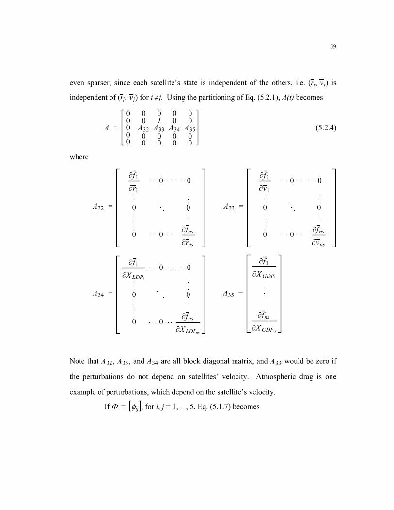
59
even sparser, since each satellite’s state is independent of the others, i.e. (ri, vi) is
independent of (rj, vj) for i ≠j. Using the partitioning of Eq. (5.2.1), A(t) becomes
A =
00000
00
A3200
0I
A3300
00
A3400
00
A3500
(5.2.4)
where
A32 =
∂f1
∂r1 0 0
0 0
0 0 ∂fns
∂rns
A33 =
∂f1
∂v1 0 0
0 0
0 0 ∂fns
∂vns
A34 =
∂f1
∂X LDP1
0 0
0 0
0 0 ∂fns
∂X LDPns
A35 =
∂f1
∂X GDP1
∂fns
∂X GDPns
Note that A32, A33, and A34 are all block diagonal matrix, and A33 would be zero if
the perturbations do not depend on satellites’ velocity. Atmospheric drag is one
example of perturbations, which depend on the satellite’s velocity.
If Φ = φij , for i, j = 1, , 5, Eq. (5.1.7) becomes

60
Φ =
0φ31B1100
0φ32B1200
0φ33B1300
0φ34B1400
0φ35B1500
(5.2.5)
where B1j = A32φ2j + A33φ3j + A34φ4j + A35φ5j for j = 1, , 5.
Integrating the first row and last two rows of Eq. (5.2.4) with the initial
conditions, Φ(t0,t0) = I yields the results that φ11=φ44=φ55=I and
φ12=φ13=φ14=φ15=φ41=φ42=φ43=φ45=φ51=φ52=φ53=φ54=0. After substituting these
results to B1j, j =1, ,5, we have
B11 = A32φ21 + A33φ31
B12 = A32φ22 + A33φ32
B13 = A32φ23 + A33φ33 (5.2.6)
B14 = A32φ24 + A33φ34 + A34
B15 = A32φ25 + A33φ35 + A35
From Eq. (5.2.5) and Eq. (5.2.6), we have
φ21 = φ31 (5.2.7a)
φ22 = φ32 (5.2.8a)

61
φ23 = φ33 (5.2.9a)
φ24 = φ34 (5.2.10a)
φ25 = φ35 (5.2.11a)
φ31 = A32φ21 + A33φ31 (5.2.7b)
φ32 = A32φ22 + A33φ32 (5.2.8b)
φ33 = A32φ23 + A33φ33 (5.2.9b)
φ34 = A32φ24 + A33φ34 + A34 (5.2.10b)
φ35 = A32φ25 + A33φ35 + A35 (5.2.11b)
From Eqs. (5.2.7a) and (5.2.7b)
φ21 - A33φ21 - A32φ21 = 0, φ21(0) = 0 φ21(0) = 0 (5.2.12)
If we define the partials of accelerations with respect to each group of parameters for
the i-th satellite as follows,
∂fi
∂ri ≡ DADRi (5.2.13a)
∂fi
∂vi ≡ DADVi (5.2.13b)

62
∂fi
∂X LDPi
≡ DLDPi (5.2.13c)
∂fi
∂X GDPi
≡ DGDPi (5.2.13d)
and φ21 is partitioned as φ21 = φ21 1, , φ21 ns
T by 3 × nkp submatrix, φ21 i, then, Eq.
(5.2.12) become
φ21 i - DADVi φ21 i - DADRi φ21 i = 0, i = 1, ,ns (5.2.14)
After applying the initial conditions, φ21 i(0) = 0 and φ21 i(0) = 0, to Eq. (5.2.14), we
have φ21 = 0. And from Eq. (5.2.7a) φ31 = 0. From Eqs. (5.2.8a) and (5.2.8b), and
Eqs. (5.2.9a) and (5.2.9b), we have similar results as follows.
φ22 i - DADVi φ22 i - DADRi φ22 i = 0, i = 1, ,ns (5.2.15)
φ23 i - DADVi φ23 i - DADRi φ23 i = 0, i = 1, ,ns (5.2.16)
with the initial conditions φ22 i(0) = I , φ22 i(0) = 0, φ23 i(0) = 0, and φ23 i(0) = I for i =
1, ,ns.
From Eqs. (5.2.10a) and (5.2.10b), we have
φ24 - A33φ24 - A32φ24 = A34, φ24(0) = 0 φ24(0) = 0 (5.2.17)
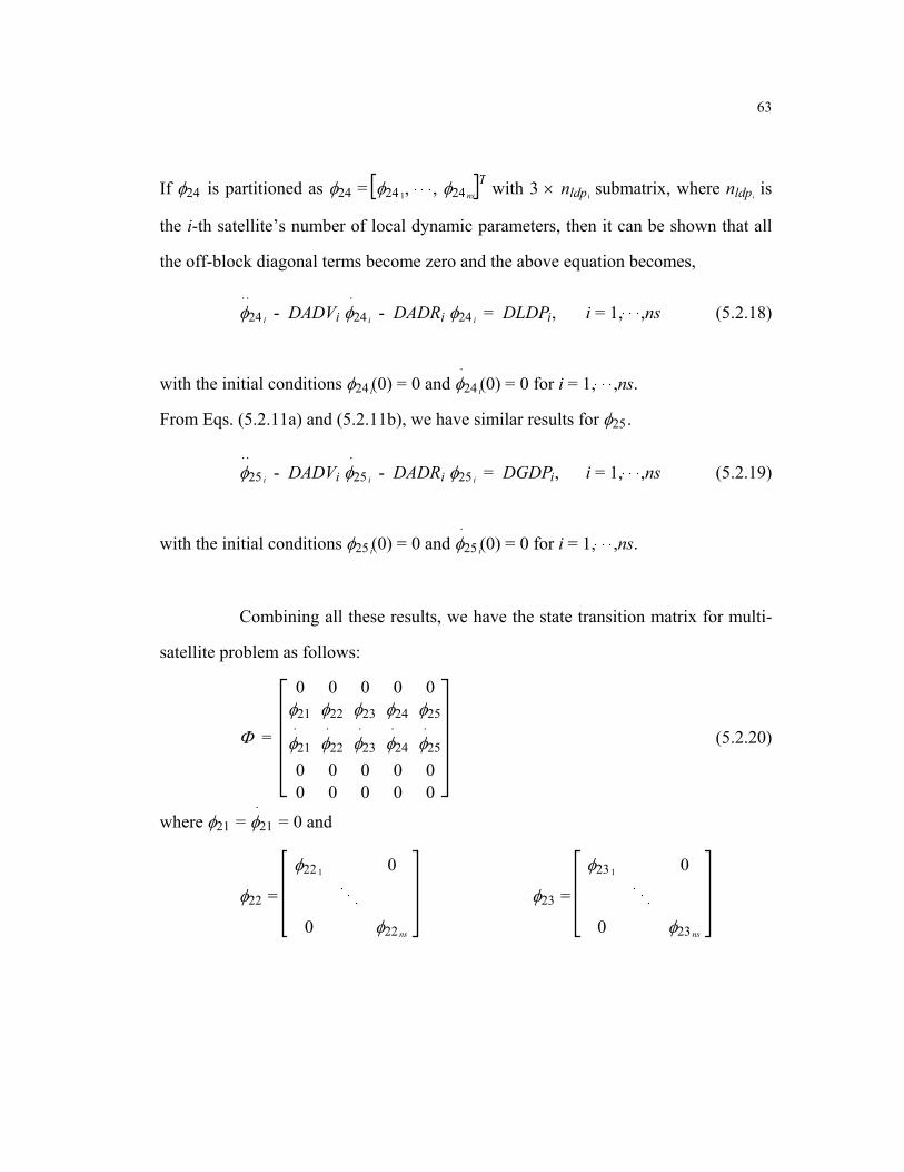
63
If φ24 is partitioned as φ24 = φ24 1, , φ24 ns
T with 3 × nldpi submatrix, where nldpi is
the i-th satellite’s number of local dynamic parameters, then it can be shown that all
the off-block diagonal terms become zero and the above equation becomes,
φ24 i - DADVi φ24 i - DADRi φ24 i = DLDPi, i = 1, ,ns (5.2.18)
with the initial conditions φ24 i(0) = 0 and φ24 i(0) = 0 for i = 1, ,ns.
From Eqs. (5.2.11a) and (5.2.11b), we have similar results for φ25.
φ25 i - DADVi φ25 i - DADRi φ25 i = DGDPi, i = 1, ,ns (5.2.19)
with the initial conditions φ25 i(0) = 0 and φ25 i(0) = 0 for i = 1, ,ns.
Combining all these results, we have the state transition matrix for multi-
satellite problem as follows:
Φ =
0φ21
φ21
00
0φ22
φ22
00
0φ23
φ23
00
0φ24
φ24
00
0φ25
φ25
00
(5.2.20)
where φ21 = φ21 = 0 and
φ22 =
φ22 1 0
0 φ22 ns
φ23 =
φ23 1 0
0 φ23 ns
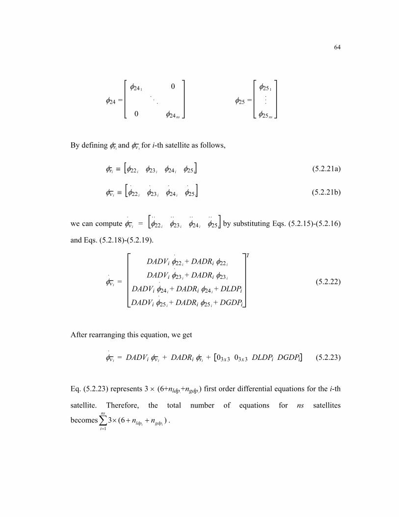
64
φ24 =
φ24 1 0
0 φ24 ns
φ25 =
φ25 1
φ25 ns
By defining φri and φv i for i-th satellite as follows,
φri ≡ φ22 i φ23 i φ24 i φ25 i (5.2.21a)
φv i ≡ φ22 i φ23 i φ24 i φ25 i (5.2.21b)
we can compute φv i = φ22 i φ23 i φ24 i φ25 i by substituting Eqs. (5.2.15)-(5.2.16)
and Eqs. (5.2.18)-(5.2.19).
φv i =
DADVi φ22 i + DADRi φ22 i
DADVi φ23 i + DADRi φ23 i
DADVi φ24 i + DADRi φ24 i + DLDPi
DADVi φ25 i + DADRi φ25 i + DGDPi
T
(5.2.22)
After rearranging this equation, we get
φv i = DADVi φv i + DADRi φri + 03x3 03x3 DLDPi DGDPi (5.2.23)
Eq. (5.2.23) represents 3 × (6+nldpi+ngdpi) first order differential equations for the i-th
satellite. Therefore, the total number of equations for ns satellites
becomes1
3 (6 )i i
ns
ldp gdpi
n n=
× + +∑ .

65
Since multi-satellite orbit determination problem includes different types
of satellites in terms of their perturbations and integration step size, a class of satellite
is defined as a group of satellites which will use the same size of geopotential
perturbation and the same integration order and step size. For l-classes of satellites,
the integration vector, X INT, is defined as

66
X INT ≡
r11
r1ns 1-----------------
φr11
φr1ns 1-----------------
v11
v1ns 1-----------------
φv11
φv1ns 1-----------------
-----------------rl1
rlns l-----------------
φrl1
φrlns l-----------------
vl1
vlns l-----------------
φvl1
φvlns l
(5.2.24)
where nsi is the number of satellites for i-th class, rij and vij are the position and
velocity of the j-th satellite of i-th class, respectively. φrij is the state transition

67
matrix for the j-th satellite’s positions of i-th class and φvij is the state transition
matrix for the j-th satellite’s velocities of i-th class.
X INT =
v11
v1ns 1-----------------
φv11
φv1ns 1-----------------
f11
f1ns 1-----------------
φv11
φv1ns 1-----------------
-----------------vl1
vlns l-----------------
φvl1
φvlns l-----------------
fl1
flns l-----------------
φvl1
φvlns l
(5.2.25)

68
Eq. (5.2.25) is numerically integrated using a procedure such as the Krogh-Shampine-
Gordon fixed-step fixed-order formulation for second-order differential equations
[Lundberg, 1981] for each class of satellites. For the ICESat/GLAS-GPS case, two
classes of satellites need to be defined. One is for the high satellites, e.g. GPS, and
the other is for the low satellite, e.g. ICESat/GLAS.
5.3 Output
Although a large number of parameters are available from the estimation
process as given by Eq. (5.2.24), the primary data product required for the generation
of other products is the ephemeris of the ICESat/GLAS spacecraft center of mass.
This ephemeris will be generated at a specified interval, e.g., 30-sec and will include
the following:
t in GPS time
3 position components of the spacecraft center of mass in ICRF and ITRF
ITRFICRFT the 3×3 transformation matrix between ICRF and the ITRF.
The output quantities will be required at times other than those contained in the
generated ephemeris file. Interpolation methods, such as those examined by
Engelkemier [1992] provide the accuracy comparable to the numerical integration
accuracy itself. With these parameters the ITRF position vector can be obtained as
well by forming the product of the transformation matrix and the position vector in
ICRF.

69
6.0 IMPLEMENTATION CONSIDERATIONS
In this chapter, some considerations for implementing ICESat/GLAS POD
algorithms are discussed. Section 6.1 describes the POD software system in which
the POD algorithms are implemented, and the necessary input files for the software
are defined. Section 6.2 describes the POD products. Section 6.3 describes the
ICESat/GLAS orbit and attitude. Section 6.4 discusses the expected ICESat/GLAS
orbit accuracy based on simulations. Section 6.5 summarizes the POD processing
strategies. Section 6.6 discusses the plans for pre-launch and post-launch POD
activities. Section 6.7 considers computational aspects.
6.1 POD Software System
The POD algorithms described in the previous chapters were implemented
in a software system, referred to as MSODP1 (Multi-Satellite Orbit Determination
Program 1). This software has been developed by the Center for Space Research
(CSR), and shares heritage with UTOPIA [Schutz and Tapley, 1980a]. This software
can process SLR data and Doppler data in addition to GPS pseudo-range and double-
differenced carrier phase data. A version of this POD software will be placed under
change control at ICESat/GLAS launch. MSODP1 requires input files, some of
which define model parameters, and the following section discusses these necessary
input files.
70
6.1.1 Ancillary Inputs
Some model parameters require continual updating through acquisition of
input information hosted on various standard anonymous ftp sites. This includes the
Earth orientation parameters, xp, yp, and UT1, and solar flux data. Other files, which
are considered to be static once "tuned" to ICESat/GLAS requirements include the
planetary ephemerides, geopotential parameters, and ocean tides parameters,. In
addition, information about the spacecraft attitude is required for the box-wing
spacecraft model in the computation of non-gravitational forces and to provide the
correction for the GPS phase center location with respect to the spacecraft center of
mass. The real-time attitude obtained during flight operations is thought to be
adequate for this purpose, but it will be checked against the precise attitude during the
Verification Phase. Also, the GPS data from the IGS ground network and the
ICESat/GLAS receiver, and SLR data from the International Laser Ranging Service
(ILRS) are needed.
6.2 POD Products
Two types of POD products will be generated: the Rapid Reference Orbit
(RRO) and the operational POD. The former product will be generated within 12-24
hours for primarily internal use of assessing the operational orbit and verification
support for mission planning. The operational POD will be generated within 14 days,
possibly within 3 days, after accounting for problems identified in RRO (e.g. GPS
satellite problems) and problems reported by IGS. This product will be used in

71
generating the altimetry standard data products, particularly level 1B and level 2
surface elevation products.
6.3 ICESat/GLAS Orbit and Attitude
During the first 30-150 days after launch, the ICESat/GLAS spacecraft
will be operated in a calibration orbit, with an 8-day repeat ground-track interval and
94-degree inclination. At some point during this period to be determined by
calibration results, the orbit will be transitioned to a neighboring mission orbit at the
same inclination, with a 183-day repeating ground track. The ICESat/GLAS
operational scenarios and orbit parameters are summarized in Table 6.1.
Table 6.1 ICESat/GLAS Orbit Parameters
Mission Phase
Expected
Duration
(days)
Mean
Altitude
(km)
Inclina-
tion
(deg)
Eccen-
tricity
Ground Track
Repeat Cycle
S/C Checkout
Calibration/
Validation
Polar Mapping
30
31-150
151-1220
600
600
600
94
94
94
0.001
0.0013
0.0013
No requirement
8 days/183 days
183 days with
25 and 8 day sub-cycles
The ICESat/GLAS spacecraft will operate in two attitude modes
depending on the angular distance between the orbit plane and the Sun (β′ angle). As
shown in Figure 1, for low-β′ periods, such as that immediately following launch, the
so-called "airplane-mode" is in use, with the solar panels perpendicular to the orbit

72
plane. When the β′ angle exceeds 32 degrees, however a yaw maneuver places the
satellite in the "sailboat-mode", with the axis of solar panels now in the orbit plane.
While the two attitudes ensure that the solar arrays produce sufficient power year-
round for bus and instrument operations, they introduce significantly different
atmospheric drag effects due to the difference in cross-sectional area perpendicular to
the velocity vector.
6.4 POD Accuracy Assessment
The predicted radial orbit errors based on recent gravity models (e.g.,
JGM-3 or EGM-96) are 19-36 cm. To reduce the effect of the geopotential model
errors on ICESat/GLAS, which is the major source of orbit error for ICESat/GLAS
POD, the gravity model improvement effort will be made through gravity tuning.
Solar activity is predicted to peak shortly after launch, and decline significantly
during the mission. The level of this activity correlates directly with the magnitude
of atmospheric drag effects on the satellite. The combinations of high solar flux and
low β′ angle at the start of the mission poses special challenges for POD and gravity
tuning.
A previous simulation study [Rim et al., 1996] indicated that the
ICESat/GLAS POD requirements could be met at 700-km altitude by either the
gravity tuning or employing frequent estimation of empirical parameters, such as
adjusting one-cycle-per-revolution parameters for every orbital revolution, within the
context of a fully dynamic approach. This approach is referred to as a highly
parameterized dynamic approach. Because the mission orbit altitude was lowered to
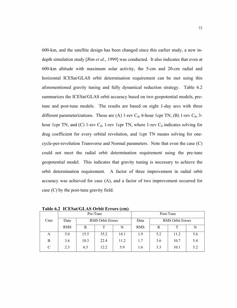
73
600-km, and the satellite design has been changed since this earlier study, a new in-
depth simulation study [Rim et al., 1999] was conducted. It also indicates that even at
600-km altitude with maximum solar activity, the 5-cm and 20-cm radial and
horizontal ICESat/GLAS orbit determination requirement can be met using this
aforementioned gravity tuning and fully dynamical reduction strategy. Table 6.2
summarizes the ICESat/GLAS orbit accuracy based on two geopotential models, pre-
tune and post-tune models. The results are based on eight 1-day arcs with three
different parameterizations. Those are (A) 1-rev Cd, 6-hour 1cpr TN, (B) 1-rev Cd, 3-
hour 1cpr TN, and (C) 1-rev Cd, 1-rev 1cpr TN, where 1-rev Cd indicates solving for
drag coefficient for every orbital revolution, and 1cpr TN means solving for one-
cycle-per-revolution Transverse and Normal parameters. Note that even the case (C)
could not meet the radial orbit determination requirement using the pre-tune
geopotential model. This indicates that gravity tuning is necessary to achieve the
orbit determination requirement. A factor of three improvement in radial orbit
accuracy was achieved for case (A), and a factor of two improvement occurred for
case (C) by the post-tune gravity field.
Table 6.2 ICESat/GLAS Orbit Errors (cm) Pre-Tune Post-Tune
RMS Orbit Errors RMS Orbit Errors
Case Data
RMS R T N
Data
RMS R T N
A
B
C
5.0
3.6
2.3
15.5
10.3
6.5
35.2
22.4
12.2
14.1
11.2
5.9
1.9
1.7
1.6
5.2
3.6
3.3
11.2
10.7
10.1
5.6
5.4
5.2

74
6.5 POD Processing Strategy
6.5.1 Assumptions and Issues
Several assumptions were made for the POD processing. We assume: 1)
continued operation of IGS GPS network and the SLR network, 2) IGS GPS data is
available in RINEX (Receiver Independent Exchange) format, 3) ICESat/GLAS GPS
receiver has performance characteristics comparable to the flight TurboRogue, and
ICESat/GLAS GPS data are available in RINEX format, and 4) most relevant IGS,
SLR and ICESat/GLAS data are available within 24-36 hours. There are several
issues for POD processing which include: 1) identification of problem GPS satellites,
2) identification of problems with ground station data, 3) processing arc length, 4)
accommodation for orbit maneuvers, and 5) problems associated with expected out-
gassing during early mission phase. For a July 2001 launch and the early phases of
the mission, orbit maneuvers are expected to occur as frequently as 5 days because of
high level of solar activity [Demarest and Schutz, 1999]. These maneuvers will not
be modeled, but the maneuver times will be utilized to reinitialize the orbit arc length.
6.5.2 GPS Data Preprocessing
The GPS data processing procedure consists of two major steps: data
preprocessing and data reduction. The data preprocessing step includes data
acquisition, correcting measurement time tags, generating double-differenced
observables, and data editing. The GPS data preprocessing system is collectively

75
called TEXGAP (university of TEXas Gps Analysis Program) and implemented on
the HP workstation.
The International GPS Service for Geodynamics (IGS) provides GPS data
collected from globally distributed GPS tracking sites, which include more than 200
ground stations at present [IGS, 1998]. The daily IGS data files are archived in the
IGS global data centers in the RINEX format, and the data from selected ground
station network will be downloaded to CSR’s data archive system. Also, the GPS
data from the ICESat/GLAS GPS receiver will be provided by the ICESat Science
Investigator Processing System.
The GPS receiver time tag is in error due to the receiver clock error, and
the time tag correction, tr, can be obtained by
tr = ρ/C – ρc/C + ts (6.1)
where C is the speed of light, ρ is the pseudorange measurement, ρc is the computed
range from GPS ephemerides and receiver position, and ts is the broadcast GPS
satellite clock correction.
Double-differencing eliminates common errors, such as the GPS satellite
and receiver clock errors, including the Selective Availability (SA) effect. As
described in Section 4.2.3, a double-differenced high-low observation consists of a
ground station, two GPS satellites, and ICESat/GLAS satellite. A careful selection of
double-differenced combination is required to avoid generating dependent data set.
To eliminate the first-order ionospheric effects, the double-differenced
carrier phase observables DDL1 at L1 and DDL2 at L2 frequency are combined to form
the ionosphere-free observable, DDLc, as follows:
2
1 1 21 22 2 2 2
1 2 1 2
L L LLc L L
L L L L
f f fDD DD DDf f f f
= −− −
(6.2)

76
where fL1 = 1575.42 MHz and fL2 = 1227.60 MHz.
Data editing involves the detection and fixing of the cycle-slips of the
carrier phase data, and the editing of data outliers. For editing outliers, a 3σ editing
criterion is applied to the double-differenced residual. Cycle-slips are detected by
examining the differences between the consecutive data points in the double-
differenced residuals and identifying discontinuity. The identified cycle-slips are
fixed by using linear extrapolations.
6.5.3 GPS Orbit Determination
ICESat/GLAS POD requires precise GPS ephemerides, and there are two
approaches to obtain the precise GPS ephemerides. The first approach is to solve the
GPS orbit simultaneously with the ICESat/GLAS orbit, and the second approach is to
fix the GPS ephemeris to an independent determination, such as the IGS solutions.
For the first approach, standard models described in Table 6.3 will be used for the
reference frame and gravitational perturbations for GPS. For the non-gravitational
perturbations on GPS, the models described in Section 3.4.5 will be employed. It has
been shown for the Topex POD case that adjusting GPS orbits usually resulted better
Topex orbit solutions [Rim et al., 1995]. A simulation study [Rim et al., 2000b]
indicates that fixing GPS orbits to high accuracy solutions would generate reasonably
well-tuned gravity field, thereby, the POD accuracy requirement could be met with
fixing GPS approach. As the accuracy of IGS solutions improved significantly
[Kouba et al., 1998], fixing GPS ephemeris to IGS solutions would be a preferred
approach for ICESat/GLAS POD. These two approaches will be evaluated using
available tracking data during the pre-launch period, such as CHAMP and JASON,

77
and ICESat/GLAS tracking data during the verification/validation period. CHAMP
POD accuracy was assessed when the GPS ephemeris is fixed to IGS solutions, such
as the ultra-rapid, rapid, and final solutions [Rim et al., 2002a]
6.5.4 Estimation Strategy
The adopted estimation strategy for ICESat/GLAS POD is the dynamic
approach with tuning of model parameters, especially the geopotential parameters.
Simulation studies indicate that frequent estimation of empirical parameters is an
effective way of reducing orbit errors. The solutions from the sequential filter with
process-noise will be investigated as a validation tool for the highly parameterized
dynamic solutions. Results of Davis [1996] and Rim et al. [2000a] show that both
highly parameterized dynamic approach with gravity tuning and the reduced-dynamic
approach yield comparable results in high fidelity simulations. This comparison will
continue with the flight data.
6.6 POD Plans
This section describes planned POD activities during the pre-launch and
the post-launch periods.
6.6.1 Pre-Launch POD Activities
During the pre-launch period, POD activities will be focused on the
following areas: 1) selection of POD standards, 2) model improvement efforts, 3)
preparation for operational POD, and 4) POD accuracy assessment. In this section,
pre-launch POD activities in these areas are summarized.

78
6.6.1.1 Standards
The standard models for the reference system, the force models and the
measurement models to be used for the ICESat/GLAS POD are described in Table
6.3. These standards are based on the International Earth Rotation Service (IERS)
Conventions [McCarthy, 1996], and the T/P standards [Tapley et al., 1994]. These
standards will be updated as the models improve, and “best” available models at
launch will be selected as the initial standard models.
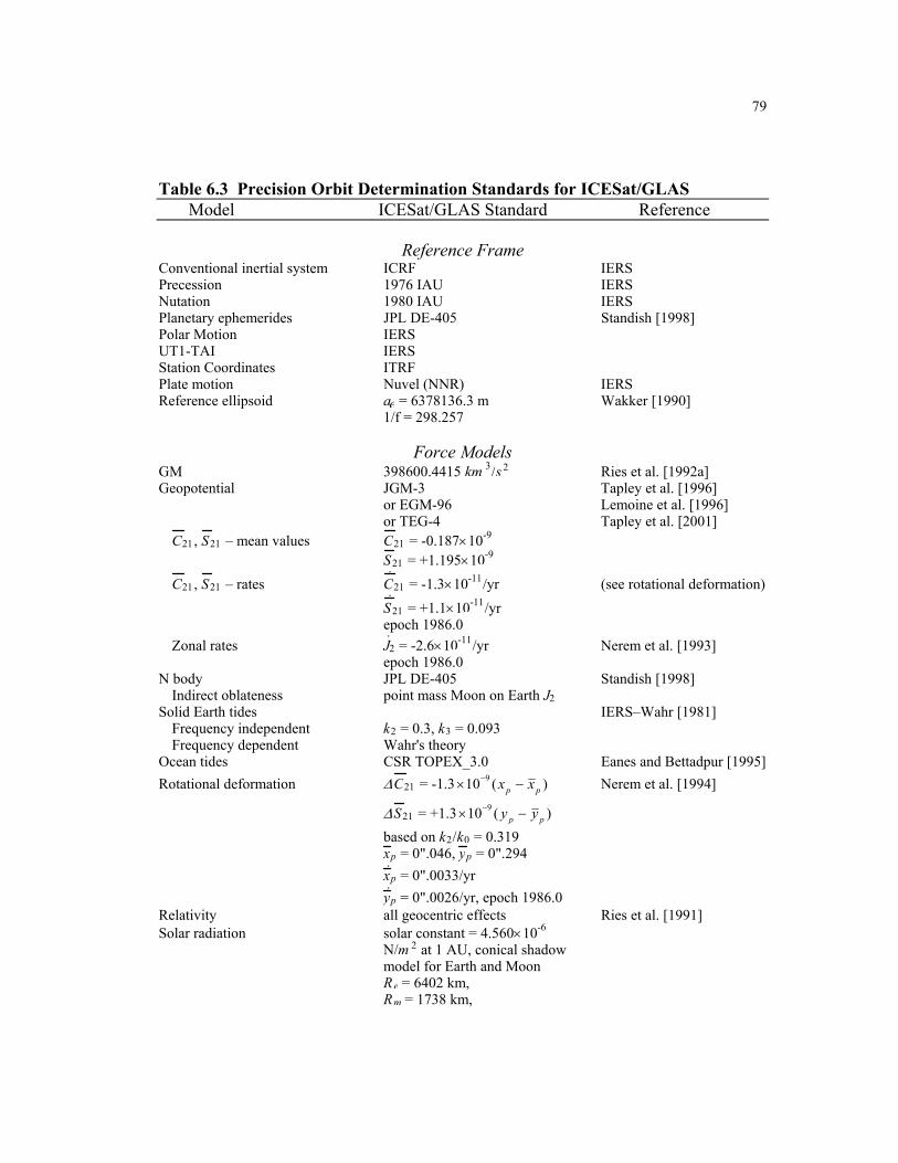
79
Table 6.3 Precision Orbit Determination Standards for ICESat/GLAS Model ICESat/GLAS Standard Reference
Reference Frame
Conventional inertial system ICRF IERS Precession 1976 IAU IERS Nutation 1980 IAU IERS Planetary ephemerides JPL DE-405 Standish [1998] Polar Motion IERS UT1-TAI IERS Station Coordinates ITRF Plate motion Nuvel (NNR) IERS Reference ellipsoid ae = 6378136.3 m Wakker [1990] 1/f = 298.257
Force Models GM 398600.4415 km 3/s 2 Ries et al. [1992a] Geopotential JGM-3 Tapley et al. [1996] or EGM-96 Lemoine et al. [1996] or TEG-4 Tapley et al. [2001] C21 , S21 – mean values C21 = -0.187×10⁻⁹ S21 = +1.195×10⁻⁹ C21 , S21 – rates C21 = -1.3×10⁻¹¹/yr (see rotational deformation) S21 = +1.1×10⁻¹¹/yr epoch 1986.0 Zonal rates J2 = -2.6×10⁻¹¹/yr Nerem et al. [1993] epoch 1986.0 N body JPL DE-405 Standish [1998] Indirect oblateness point mass Moon on Earth J2 Solid Earth tides IERS–Wahr [1981] Frequency independent k2 = 0.3, k3 = 0.093 Frequency dependent Wahr's theory Ocean tides CSR TOPEX_3.0 Eanes and Bettadpur [1995] Rotational deformation ∆C21 = -1.3 910 ( )p px x−× − Nerem et al. [1994]
∆S21 = +1.3 910 ( )p py y−× − based on k2/k0 = 0.319 xp = 0".046, yp = 0".294 xp = 0".0033/yr yp = 0".0026/yr, epoch 1986.0 Relativity all geocentric effects Ries et al. [1991] Solar radiation solar constant = 4.560×10⁻⁶ N/m 2 at 1 AU, conical shadow model for Earth and Moon Re = 6402 km, Rm = 1738 km,
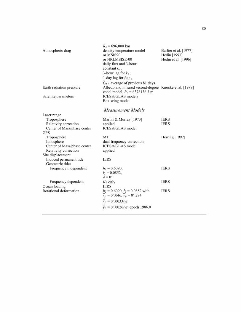
80
Rs = 696,000 km Atmospheric drag density temperature model Barlier et al. [1977] or MSIS90 Hedin [1991] or NRLMSISE-00 Hedin et al. [1996] daily flux and 3-hour constant kp, 3-hour lag for kp; 1-day lag for f10.7 , f10.7 average of previous 81 days Earth radiation pressure Albedo and infrared second-degree Knocke et al. [1989] zonal model, Re = 6378136.3 m Satellite parameters ICESat/GLAS models Box-wing model
Measurement Models Laser range Troposphere Marini & Murray [1973] IERS Relativity correction applied IERS Center of Mass/phase center ICESat/GLAS model GPS Troposphere MTT Herring [1992] Ionosphere dual frequency correction Center of Mass/phase center ICESat/GLAS model Relativity correction applied Site displacement Induced permanent tide IERS Geometric tides Frequency independent h2 = 0.6090, IERS l2 = 0.0852, δ = 0° Frequency dependent K1 only IERS Ocean loading IERS Rotational deformation h2 = 0.6090, l2 = 0.0852 with IERS xp = 0".046, yp = 0".294 xp = 0".0033/yr yp = 0".0026/yr, epoch 1986.0

81
Figures 2 and 3 show the ground station network for ICESat/GLAS POD
for GPS and SLR, respectively. Details of the adopted network may change prior to
launch but will remain quite robust. Station coordinates will be adopted from the
"best" available ITRF model, expected to be ITRF-99 or ITRF-2000. The ITRF
model includes station velocities measured by space geodetic methods.
6.6.1.2 Gravity Model Improvements
The gravity model to be used in the immediate post-launch period will be
"best" available at launch, such as JGM-3 [Tapley et al., 1996], EGM-96 [Lemoine et
al., 1996], or TEG-4 [Tapley et al., 2001]. As further gravity model improvements
are made from other projects, such as GRACE, they will be incorporated for
ICESat/GLAS POD. At this writing, further study is required for the selection of the
at-launch gravity model. However, current state-of-the-art models are sufficiently
close that geopotential tuning with ICESat/GLAS data should yield comparable POD
performance which is largely unaffected by this initial selection. The “best” available
ocean tide model at launch will be adopted as the standard ocean tide model for
ICESat/GLAS POD.
6.6.1.3 Non-Gravitational Model Improvements
Since the ICESat/GLAS launch coincides with the predicted solar
maximum, the atmospheric drag perturbation will be the largest non-gravitational
force acting on the satellite. Some drag-related models were evaluated for CHAMP
POD, as part of drag model improvement efforts for reducing the effect of drag model
errors on ICESat/GLAS POD [Rim et al., 2002b]. Those include the thermospheric

82
wind model, HWM93, NRLMSISE-00 [Hedin et al., 1996], and DTM-2000
[Bruinsma and Thuillier, 2000]. Estimation strategies to minimize the effects of drag
model errors on POD and gravity tuning will also be investigated.
In order of decreasing magnitude, the remaining non-gravitational
perturbations consist of solar radiation pressure, Earth radiation pressure, and on-
board thermal emission. For POD, a 'box-wing' model, described in Section 3.4.6,
represents the spacecraft as a simple combination of a six-sided box and two attached
panels, or 'wings'. This macro-model will use effective specular and diffuse
reflectivity coefficients to compute the induced forces acting on each surface. The
pre-flight values of these coefficients will be estimated during a tuning process, in
which the forces computed with the macro-model are fit to those obtained using a
separate micro-model [Webb, private communication, 2000]. This latter model
employs considerable detail that makes it impractical for use directly in POD. Once
ICESat/GLAS is in orbit, the reflectivity coefficients will be adjusted during POD,
using the GPS tracking data.
The macro-model tuning effort will compute the radiation from various
sources incident on the satellite's surfaces. By using a comprehensive thermal model,
the propagation of this energy throughout the spacecraft will be calculated. The
resulting temperature distribution will be evaluated to determine whether any on-
board thermal gradients may induce net forces. Any such forces would then be
modeled analytically during POD.
The non-gravitational forces acting on each surface due to atmospheric
drag, solar radiation pressure, Earth radiation pressure, and thermal emission are

83
computed individually and then summed to obtain the total non-gravitational force
acting on the satellite.
6.6.1.4 Measurement Model Developments
One of the sources of measurement model errors is the multipath effect.
Colorado Center for Astrodynamics Research (CCAR) multipath study [Axelrad et
al., 1999] indicates that the multipath effect alone results in 1-2 cm radial orbit error,
while this effect in the presence of other errors, such as drag and gravitational model
errors, results in a few mm error. This study was based on a preliminary design
location for the antennas and most of the multipath effect was caused by the solar
arrays. It also indicates that the effect becomes even smaller with proper editing
scheme, such as blocking certain regions. The capability of screening out GPS
measurements from blocked regions was implemented in MSODP1. Strategies for
detecting and mitigating the multipath effect on CHAMP POD were investigated
[Yoon et al., 2002b], and similar approach will be adopted for ICESat/GLAS POD.
The final spacecraft design has the GPS antennas positioned above the solar array and
bus star cameras. In this location, there is no expected impingement above the
ground plane so multipath will be mitigated.
ICESat/GLAS satellite’s center of mass location with respect to a
reference point on the spacecraft will be measured in the pre-launch period, and the
location of the GPS antenna and the laser reflector will also be measured. GPS
antenna phase center variations as a function of azimuth and elevation will be
determined in pre-launch testing. Effect of GPS antenna phase center variation on

84
POD was investigated using CHAMP data [Yoon et al., 2002a]. Expenditure of fuel
and corresponding changes in center of mass location will be monitored during flight.
6.6.1.5 Preparation for Operational POD
To generate the POD products operationally when large volumes of data
are required, it is essential to make the POD processing as automatic as possible. The
POD processing procedures will be examined end-to-end to identify/update the
procedures for possible improvement and to minimize the human intervention, and
computational and human resources will be allocated optimally for POD processing.
The adopted operational POD processing procedures/scripts will be tested by
processing upcoming satellites, such as JASON and CHAMP, during the pre-launch
period for further improvement.
6.6.1.6 Software Comparison
Since the POD products from different software will be compared for
POD validation, it is important to compare different software packages in the pre-
launch period to identify model differences and to quantify the level of agreement
among different POD software systems, such as UT-CSR’s MSODP1, GSFC’s
GEODYN, and JPL’s GOA II. This comparison becomes easier for the
ICESat/GLAS POD due to the extensive POD software comparison activity between
UT-CSR and GSFC for Topex POD [Ries, 1992b]. Also, Topex-GPS POD
experiments between UT-CSR and JPL [Bertiger et al., 1994] gave the opportunity
for both groups to compare their software systems. This comparison will continue for
the ICESat/GLAS POD models to ensure the validity of the POD verification by
comparing with POD products from different software systems.

85
6.6.1.7 POD Accuracy Assessment
During the pre-launch period, simulation studies will continue to assess
the POD accuracy. Comparison of highly parameterized dynamic approach and the
reduced-dynamic approach will be continued. For the GPS orbit modeling, standard
models for GPS orbit determination will be updated as the models progress, and the
resulting orbit will be compared to the IGS solutions. Also, the effect of fixing GPS
orbits to independently determined ephemerides, such as IGS solutions, on the POD
and the gravity tuning will be evaluated.
6.6.2 Post-Launch POD Activities
During the first 30-150 days after launch, which is the
Calibration/Validation period, POD processing will tune the model parameters,
including the gravity, and define adopted parameter set for processing the first 183-
day cycle. During the 183 days of the Cycle 1, the POD processing will assess and
possibly further improve or refine parameters, such as assess the gravity field from
the gravity mission GRACE, if available, and adopt a new parameter set for the
processing of Cycle 2 data. POD processing will continue assessment of POD quality
after Cycle 1, and new parameter adoptions should be minimized and timed to occur
at cycle boundaries.
6.6.2.1 Verification/Validation Period
During the calibration/validation period, several important POD activities
will be undertaken simultaneously. These include tuning model parameters, POD
calibration/validation, evaluation of out-gassing effect, evaluation of estimation

86
strategies and GPS orbit modeling procedure, evaluation of multipath effect and
construction of editing scheme.
Some model parameters, such as geopotential parameters and the “box-
wing” model parameters, will be tuned using the tracking data. About 30-40 days of
GPS data will be processed for gravity tuning, and the arc length will be dictated by
the maneuver spacing and the ability of POD to mitigate the effect of the non-
gravitational model errors, especially the drag model errors, to certain level. The
tuned gravity field will be determined by combining the pre-tune gravity coefficients
and the solution covariance with the new information equations from the GPS
tracking data.
Internal and external POD calibration/validation activities are planned for
POD quality assessment, and those are summarized in the following section.
During the early phase of the mission, the satellite might experience
significant out-gassing, and this poses serious challenges for POD. However, this
effect will subside as time goes by, and every effort will be made to insure that this
effect does not corrupt the parameter tuning process during this
validation/verification period.
Estimation strategies described in Section 6.5.4 will be evaluated, and the
GPS orbit modeling procedures described in Section 6.5.3 will also be evaluated
during this period.
The multipath effect will be evaluated to characterize the extent of signal
corruption due to diffraction and reflection using the flight data. Proper editing
scheme will be developed if there is any evidence that such an editing reduces the
multipath effect on POD.

87
6.6.2.2 POD Product Validation
To validate the accuracy of ICESat/GLAS POD products, several methods
would be employed. For the internal evaluation of the orbit consistency, orbit
overlap statistics will be analyzed. Also, the data fit RMS value is an effective
indicator of orbit quality. Comparisons between the orbits from different software,
such as MSODP1, GEODYN, and GIPSY-OASIS II (GOA II), would serve as a
valuable tool to assess the orbit accuracy. Since the ICESat/GLAS will carry the
laser reflector on board, the SLR data can be used as an independent data set to
determine the ICESat/GLAS orbit. However, this approach assumes reasonably good
tracking of the ICESat/GLAS orbit from the SLR stations. Data from the SLR
network will also be used to directly evaluate the GPS-determined orbit. Data fits for
high elevation SLR passes can be used to evaluate the orbit accuracy of the
ICESat/GLAS. The laser altimeter data will be used to assess the validation,
however, this assessment can be accomplished only if the calibration and verification
of the instrument have been accomplished. Global crossovers from ICESat/GLAS
will be used to validate the radial orbit accuracy in a relative sense.
6.6.2.3 POD Reprocessing
To produce improved orbits, reprocessing of data will be performed as
often as annually. As the solar activity is expected to decrease in the later mission
period, the accuracy of the tuned model parameters will be improved, thereby the
POD accuracy will be improved. Any improvement in the model parameters will be
adopted for the reprocessing.

88
6.7 Computational: CPU, Memory and Disk Storage
Table 6.4 compares the computational requirements for processing a
typical one-day arc from a 24-ground station network with 30 sec sampling time for
both T/P and ICESat/GLAS. These results are based on MSODP1 implemented on
the Cray J90 and the HP-735/125.
Current computational plans are to use the HP-class workstation
environment for preprocessing GPS data, including generation of double difference
files. POD processing will be performed on a Cray J90, or equivalent. This
processing on the Cray enables a more efficient resource sharing with other project,
such as GRACE.
Table 6.4 Computational Requirements for T/P and ICESat/GLAS POD using
MSODP1: One-day Arcs with 24 Ground Stations
Platform Satellite CPU (min) Memory (Mw) Disk∗ (Mb)
T/P 20 2 35 Cray J90
ICESat/GLAS 40 2.5 59
T/P 30 2 39 HP-735
ICESat/GLAS 105 2.5 63
∗ This includes all the necessary files.

89
a) "airplane mode" for low β′
b) "sailboat mode" for high β′
Figure 1. ICESat/GLAS Operational Attitudes
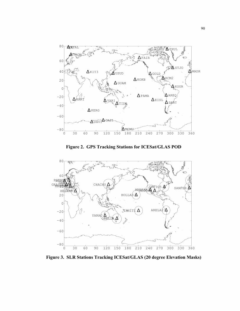
90
-80
80
-60
-40
-20
0
20
40
60
0 36030 60 90 120 150 180 210 240 270 300 330
∆ TROM
∆ NYAL
∆KIT3 ∆ MADR ∆USUD
∆HART
∆ STJO
∆GOLD
∆FAIR
∆ KOKB ∆RCM2
∆EISL ∆SANT
∆AREQ
∆TIDB ∆YAR1
∆ GUAM
∆ MCMU
∆ DAV1 ∆ CAS1
∆ KERG
∆ PAMA
∆KOUR
∆ THUL
Figure 2. GPS Tracking Stations for ICESat/GLAS POD
-80
80
-60
-40
-20
0
20
40
60
0 36030 60 90 120 150 180 210 240 270 300 330
∆ MCDON4
∆ YARAG
∆ GRF105∆ MNPEAK
∆ TAHITI
∆ HOLLAS
∆ CHACHU
∆ ARELA2
∆ SANFER∆ HELWAN
∆ GRASSE∆ POTSD2 ∆ GRAZ∆ RGO
∆ ORRLLR
∆ MATERA
Figure 3. SLR Stations Tracking ICESat/GLAS (20 degree Elevation Masks)

91
7.0 BIBLIOGRAPHY
Anderle, R. J., Geodetic Analysis Through Numerical Integration, Proceedings of the
International Symposium on the Use of Artificial Satellites for Geodesy and
Geodynamics, Athens, Greece, 1973.
Antreasian, P. G. and G. W. Rosborough, Prediction of Radiant Energy Forces on the
TOPEX/POSEIDON Spacecraft, J. Spacecraft and Rockets, Vol. 29, No. 1,
81-90, 1992.
Atlshuler, E. E., and P. M. Kalaghan, Tropospheric range error corrections for the
NAVSTAR system, Air Force Cambridge Research Laboratories, AFCRL-TR-
74-0198, April 1974.
Axelrad, P., K. Gold, P. Madhani, ICESat Observatory Multipath Effect, Final
Report, Colorado Center for Astrodynamics Research, University of
Colorado, March, 1999.
Barlier, F., C. Berger, J. L. Falin, G. Kockarts, and G. Thuiller, A Thermospheric
Model Based on Satellite Drag Data, Aeronomica Acta, Vol. 185, 1977.
Bertiger, W. I., Y. E. Bar-Sever, E. J. Christensen, E. S. Davis, J. R. Guinn, B. J.
Haines, R. W. Ibanez-Meier, J. R. Jee, S. M. Lichten, W. G. Melbourne, R. J.
Mullerschoen, T. N. Munson, Y. Vigue, S. C. Wu, T. P. Yunck, B. E. Schutz,
P. A. M. Abusali, H. J. Rim, M. M. Watkins, and P. Willis, GPS Precise
Tracking of TOPEX/POSEIDON: Results and Implications, J. Geophys. Res.,
99, C12, 24449-24464, 1994.

92
Beutler, G., E. Brockmann, U. Gurtner, L. Hugentobler, L. Mervart, M. Rothacher,
and A. Verdun, Extended Orbit Modeling Techniques at the CODE
Processing Center of the International GPS Service for Geodynamics (IGS):
Theory and the Initial Results, Manuscripta Geodaetica, 19, 367-386, 1994.
Bruinsma, S. L., and G. Thuillier, A Revised DTM Atmospheric Density Model:
Modeling Strategy and Results, EGS XXV General Assembly, Session G7,
Nice, France, 2000.
Byun, S. H., Satellite Orbit Determination Using GPS Carrier Phase in Pure
Kinematic Mode, Dissertation, Department of Aerospace Engineering and
Engineering Mechanics, The University of Texas at Austin, December, 1998.
Cartwright D. E. and R. J. Tayler, New Computations of the Tide Generating
Potential, Geophys. J. Roy. Astron. Soc., Vol. 23, 45-74, 1971.
Cartwright D. E. and A. C. Edden, Corrected Tables of Tidal Harmonics, Geophys. J.
Roy. Astron. Soc., Vol. 33, 253-264, 1973.
Cassoto, S., Ocean Tide Models for Topex Precise Orbit Determination, Dissertation,
Department of Aerospace Engineering and Engineering Mechanics, The
University of Texas at Austin, December 1989.
Chao, C. C., The Tropospheric Calibration Model for Mariner Mars 1971, Technical
Report 32-1587, 61-76, JPL, Pasadena, California, March, 1974.
93
Christensen, E. J., B. J. Haines, K. C. McColl, and R. S. Nerem, Observations of
Geographically Correlated Orbit Errors for TOPEX/Poseidon Using the
Global Positioning System, Geophys. Res. Let., 21(19), 2175-2178, Sep. 15,
1994.
Ciufolini, I., Measurement of the Lense-Thirring Drag on High-Altitude Laser-
Ranged Artificial Satellites, Phys. Rev. Let., 56, 278, 1986.
Clynch J. R. and D. S. Coco, Error Characteristics of High Quality Geodetic GPS
Measurements: Clocks, Orbits, and Propagation Effects, in Proceedings of the
4th International Geodetic Symposium on Satellite Positioning, Austin, Texas,
1986.
Colombo, O. L., Ephemeris Errors of GPS Satellites, Bull. Geod., 60, 64-84, 1986.
Colombo, O. L., The Dynamics of Global Positioning System Orbits and the
Determination of Precise Ephemerides, J. Geophys. Res., 94, B7, 9167-9182,
1989.
Davis, G. W., GPS-Based Precision Orbit Determination for Low Altitude Geodetic
Satellites, CSR-96-1, May 1996.
Demarest, P. and B. E. Schutz, Maintenance of the ICESat Exact Repeat Ground
Track, Proc. AAS/AIAA Astrodynamics Specialist Conference, Paper AAS 99-
391, Girdwood, Alaska, August 16-19, 1999.

94
DeMets, C., R. G. Gordon, D. F. Argus, and S. Stein, Current Plate Motions, Geophys
J. R. Astron. Soc., 1990.
Dow, J. M., Ocean Tide and Tectonic Plate Motions from Lageos, Dissertation, Beim
Fachbereich 12 - Vermessungswesen, der Technishen Hochshule Darmstadt,
Munchen, 1988.
Eanes, R. J., B. E. Schutz, and B. D. Tapley, Earth and Ocean Tide Effects on Lageos
and Starlette, Proceedings of the Ninth International Symposium on Earth
Tides (Ed. J. T. Kuo), 239-249, 1983.
Eanes, R. J. and S. Bettadpur, The CSR 3.0 Global Ocean Tide Model Diurnal and
Semi-diurnal Ocean Tides from TOPEX/Poseidon Altimetry, CSR-TM-96-06,
1995.
Engelkemier, B. S., Lagrangian Interpolation to an Ordered Table to Generate a
Precise Ephemeris, Thesis, The University of Texas at Austin, 1992.
Elyasberg, P., B. Kugaenko, V. Synitsyn, and M. Voiskovsky, Upper Atmosphere
Density Determination from the COSMOS Satellite Deceleration Results,
Space Research, Vol. XII, 1972.
Feulner, M. R., The Numerical Integration of Near Earth Satellite Orbits Across SRP
Boundaries Using the Method of Modified Back Differences, Thesis,
Department of Aerospace Engineering and Engineering Mechanics, The
University of Texas at Austin, August 1990.
95
Finn, A. and J. Matthewman, A Single-Frequency Ionospheric Refraction Correction
Algorithm for TRANSIT and GPS, in Proceedings of the 5th International
Geodetic Symposium on Satellite Positioning, Las Cruces, New Mexico,
March 13-17, 1989.
Fliegel H. F., T. E. Gallini, and E. R. Swift, Global Positioning System Radiation
Force Model for Geodetic Applications, J. Geophys. Res., 97, 559-568, 1992.
Gibson, L. R., A Derivation of Relativistic Effect in Satellite Tracking, Technical
Report 83-55, NSWC, Dahlgren, Virginia, April, 1983.
Goad, C. C. and L. Goodman, A Modified Hopfield Tropospheric Refraction
Correction Model, presented at the AGU Fall Meeting, San Francisco, Calif.,
December 1974.
Goad, C. C., Gravimetric Tidal Loading Computed from Integrated Green’s
Functions, J. Geophys. Res., 85, 2679-2683, 1980.
Hedin, A. E., Extension of the MSIS Thermosphere and Exosphere with Empirical
Temperature Profiles, J. Geophys. Res., 96, 1159-1172, 1991.
Hedin, A. E., E. L. Fleming, A. H. Manson, F. J. Schmidlin, S. K. Avery, R. R. Clark,
S. J. Franke, G. J. Fraser, T. Tsuda, F. Vidal, and R. A. Vincent, Empirical
Wind Model for the Upper, Middle and Lower Atmosphere, J. Atmos. Terr.
Phys., 58, 1421-1447, 1996.

96
Heiskanen, W. A. and H. Moritz, Physical Geodesy, W. H Freeman and Company,
London, 1967.
Herring, T. A., B. A. Buffett, P. M. Mathews, and I. I. Shapiro, Forced Nutations of
the Earth: Influence of Inner Core Dynamics 3. Very Long Interferometry
Data Analysis, J. Geophys. Res., 96, 8259-8273, 1991.
Herring, T. A., Modeling Atmospheric Delays in the Analysis of Space Geodetic
Data, in Refraction of Transatmospheric Signals in Geodesy, J. De Munck and
T. Spoelstra (ed.), Netherland Geodetic Commission Publications in Geodesy,
36, 157-164, 1992.
Hofmann-Wellenhof, B., H. Lichtenegger, and J. Collins, GPS Theory and Practice,
Springer-Verlag Wien, New York, 1992.
Holdridge, D. B., An Alternate Expression for Light Time Using General Relativity,
JPL Space Program Summary 37-48, III, 2-4, 1967.
Huang, C. and J. C. Ries, The Effect of Geodesic Precession in the Non-Inertial
Geocentric Frame, CSR-TM-87-04, Center for Space Research, The
University of Texas at Austin, December, 1987.
Huang, C., J. C. Ries, B. D. Tapley, and M. M. Watkins, Relativistic Effects for Near-
Earth Satellite Orbit Determination, Celestial Mechanics, Vol. 48, No. 2, 167-
185, 1990.
IGS, International GPS Service for Geodynamics: Resource information, 1998.

97
Jacchia, L. G., Revised Static Models of the Thermosphere and Exosphere with
Empirical Temperature Profiles, Smith. Astrophys. Obs. Spec. Rep., 332,
1971.
Jacchia, L. G., Thermospheric Temperature Density, and Composition: New Models,
Smith. Astrophys. Obs. Spec. Rep., 375, 1977.
Kaula, W. M., Theory of Satellite Geodesy, Blaisdell, Waltham, Mass., 1966.
Knocke, P. C. and J. C. Ries, Earth Radiation Pressure Effects on Satellites,
University of Texas Center for Space Research Technical Memorandum,
CSR-TM-87-01, September, 1987.
Knocke, P. C., Earth Radiation Pressure Effects on Satellite, Dissertation, Department
of Aerospace Engineering and Engineering Mechanics, The University of
Texas at Austin, May, 1989.
Kouba, J., Y. Mireault, G. Beutler, T. Springer, and G. Gendt, A Discussion of IGS
Solutions and Their Impact on Geodetic and Geophysical Applications, GPS
Solutions, Vol. 2, No. 2, 3-15, Fall 1998.
Lambeck, K., The Earth’s Variable Rotation: Geophysical Causes and
Consequences, Cambridge University Press, 1980.
Lawson, C. L. and R. J. Hanson, Solving Least Squares Problems, Prentice-Hall Inc.,
Englewood Cliffs, New York, 1974.

98
Lemoine, F. G., E. C. Pavlis, S. M. Klosko, N. K. Pavlis, J. C. Chan, S. Kenyon, R.
Trimmer, R. Salman, R. H. Rapp, and R. S. Nerem, Latest Results from the
Joint NASA GSFC and DMA Gravity Model Project, EOS Transactions,
AGU, 77(17), p. S41, 1996.
Lieske, J. H., T. Lederle, W. Fricke, and B. Morando, Expressions for the precession
quantities based upon the IAU (1976) System of Astronomical Constants,
Astronomy and Astrophysics, Vol. 58, 1-16, 1977.
Lieske, J. H. Precession matrix based on IAU (1976) system of astronomical
constants, Astronomy and Astrophysics, Vol. 73, 282-284, 1979.
Lundberg, J. B., Numerical Integration Techniques for Satellite Orbits, Univ. of
Texas at Austin, Department of Aerospace Engineering and Engineering
Mechanics, IASOM-TR-81-1, 1981.
Lundberg, J. B., Computational Errors and their Control in the Determination of
Satellite Orbits, Report CSR-85-3, The Center for Space Research, The
University of Texas at Austin, 1985.
Marini, J. W. and C. W. Murray, Correction of Laser Range Tracking Data for
Atmospheric Refraction at Elevations above 10 Degrees, Rep. X-591-73-351,
Goddard Space Flight Center, Greenbelt, Maryland, November 1973.

99
Marshall, J. A., S. B. Luthcke, P. G. Antreasian, and G. W. Rosborough, Modeling
Radiation Forces Acting on TOPEX/Poseidon for Precise Orbit
Determination, NASA Technical Memorandom 104564, June 1992.
McCarthy J. J. and T. V. Martin, A Computer Efficient Model of Earth Albedo
Satellite Effects, NASA Goddard Space Flight Center, Planetary Sciences
Department Report No. 012-77, June, 1977.
McCarthy D. D. (Ed.), IERS Conventions (1996), IERS Tech. Note 21, Obs. de Paris,
July 1996.
Melbourne, W. G., E. S. Davis, T. P. Yunck, and B. D. Tapley, The GPS Flight
Experiment on TOPEX/Poseidon, Geophys. Res. Let., Vol. 21, No. 19, 2171-
2174, Sep. 15, 1994.
Milani, A., Non-Gravitational Perturbations and Satellite Geodesy, Adam Hilger,
1987.
Milliken, R. J. and C. J. Zoller, Principle of Operation of NAVSTAR and System
Characteristics, Navigation, Vol. 25, 95-106, 1978.
Minster, J. B., and T. H. Jordan, Present Day Plate Motions, J. Geophys. Res., 83,
5331-5354, 1978.
Moyer, T. D., Transformation from Proper Time on Earth to Coordinate Time in
Solar System Barycentric Space-Time Frame of Reference. Part 1 & Part 2,
Celestial Mechanics, Vol. 23, 33-56, 57-68, 1981.

100
Nerem, R. S., B. F. Chao, A. Y. Au, J. C. Chan, S. M. Klosko, N. K. Pavlis, and R. G.
Williamson, Time Variations of the Earth’s Gravitational Field from Satellite
Laser Ranging to LAGEOS, Geophys. Res. Lett., 20(7), 595-598, 1993.
Nerem, R. S., F. J. Lerch, J. A. Marshall, E. C. Pavlis, B. H. Putney, B. D. Tapley, R.
J. Eanes, J. C. Ries, B. E. Schutz, C. K. Shum, M. M. Watkins, S. M. Klosko,
J. C. Chan, S. B. Luthcke, G. B. Patel, N. K. Pavlis, R. G. Williamson, R. H.
Rapp, R. Biancale, and F. Nouel, Gravity Model Development for
TOPEX/POSEIDON: Joint Gravity Models 1 and 2, J. of Geophys. Res., 99,
24421-24447, 1994.
Remondi, B. W., Using the Global Positioning System (GPS) Phase Observable for
Relative Geodesy: Modeling, Processing, and Results, Dissertation,
Department of Aerospace Engineering and Engineering Mechanics, The
University of Texas at Austin, May, 1984.
Ries, J. C., C. Huang, and M. M. Watkins, Effect of General Relativity on a near-
Earth satellite in the geocentric and barycentric reference frames, Phys. Rev.
Lett., 61, 903, 1988.
Ries, J. C., Simulation of an Experiment to Measure the Lense-Thirring Precession
Using a Second Lageos Satellite, Dissertation, Department of Aerospace
Engineering and Engineering Mechanics, The University of Texas at Austin,
December, 1989.

101
Ries, J. C., C. Huang, M. M. Watkins, and B. D. Tapley, Orbit Determination in the
Relativistic Geocentric Reference Frame, J. Astron. Sci., 39(2), 173-181,
1991.
Ries, J. C., R. J. Eanes, C. K. Shum, and M. M. Watkins, Progress in the
Determination of the Gravitational Coefficients of the Earth, Geophys. Res.
Lett., 19(6), 529-531, 1992a.
Ries, J. C. and D. Pavlis, TOPEX/POSEIDON Project, Software Intercomparison
Results – Phase I and II, The University of Texas Center for Space Research,
March 1992b.
Rim, H. J., B. E. Schutz, P. A. M. Abusali, and B. D. Tapley, Effect of GPS Orbit
Accuracy on GPS-determined TOPEX/Poseidon Orbit, Proc. ION GPS-95,
613-617, Palm Springs, California, Sep. 12-15, 1995.
Rim, H. J., G. W. Davis, and B. E. Schutz, Dynamic Orbit Determination for the EOS
Laser Altimeter Satellite (EOS ALT/GLAS) Using GPS Measurements, J.
Astron. Sci., 44(3), 409-424, 1996.
Rim, H. J., C. Webb, and B. E. Schutz, Analysis of GPS and Satellite Laser Ranging
(SLR) Data for ICESat Precision Orbit Determination, Proc. AAS/AIAA Space
Flight Mechanics Meeting, Paper 99-146, Breckenridge, Colorado, February
7-10, 1999.

102
Rim, H. J., C. Webb, S. Byun, and B. E. Schutz, Comparison of GPS-Based Precision
Orbit Determination Approaches for ICESat, Proc. AAS/AIAA Space Flight
Mechanics Meeting, Paper AAS-00-114, Clearwater, Florida, Jan. 24-26,
2000a.
Rim, H. J., C. Webb, and B. E. Schutz, Effect of GPS Orbit Errors on ICESat
Precision Orbit Determination, Proc. AIAA/AAS Astrodynamics Specialist
Conference, Paper AIAA-2000-4234, Denver, Colorado, Aug. 14-17, 2000b.
Rim, H. J., S. Yoon, and B. E. Schutz, Effect of GPS Orbit Accuracy on CHAMP
Precision Orbit Determination, AAS/AIAA Space Flight Mechanics Meeting,
Paper AAS 02-213, San Antonio, Texas, Jan. 27-30, 2002a.
Rim. H. J., Y. C. Kim, and B. E. Schutz, Atmospheric Drag Modeling for CHAMP
Precision Orbit Determination, Proc. AIAA/AAS Astrodynamics Specialist
Conference, Paper No. 2002-4737, Monterey, CA, Aug. 5-8, 2002b.
Schutz, B. E., and B. D. Tapley, Utopia: University of Texas Orbit Processor,
Department of Aerospace Engineering and Engineering Mechanics, The
University of Texas at Austin, TR 80-1, 1980a.
Schutz, B. E., and B. D. Tapley, Orbit Accuracy Assessment for Seasat, J. Astron.
Sci., Vol. XXVIII, No. 4, 371-390, October-December, 1980b.

103
Schutz, B. E., B. D. Tapley, R. J. Eanes, and M. M. Watkins, Earth Rotation from
Lageos Laser Ranging, Bureau International De L’Heure (BIH) Annual
Report, D51-D56, July, 1988.
Schutz, B. E., B. D. Tapley, P. A. M. Abusali, and H. J. Rim, Dynamic Orbit
Determination Using GPS Measurements from TOPEX/Poseidon, Geophys.
Res. Let., 21(19), 2179-2182, Sep. 15, 1994.
Seidelmann, P. K., 1980 IAU Theory of Nutation: The Final Report of the IAU
Working Group on Nutation, Celestial Mechanics, Vol. 27, 79-106, 1982.
Shum, C. K., J. C. Ries, B. D. Tapley, P. Escudier, and E. Delaye, Atmospheric Drag
Model for Precise Orbit Determination, CSR-86-2, Center for Space Research,
The University of Texas of Austin, 1986.
Spilker, J. J., Jr., GPS Signal Structure and Performance Characteristics, Navigation,
Vol. 25, 121-146, 1978.
Springer, T. A., G. Beutler and M. Rothacher, A New Solar Radiation Pressure
Model for the GPS Satellites, IGS Workshop Proceedings, Darmstadt,
Germany, ESOC, 1998.
Standish, E. M., JPL Planetary and Lunar Ephemerides DE405/LE405, JPL
Interoffice Memorandum, IOM 312.F-98-048, Aug. 26, 1998 (Ephemerides
available on CD-ROM).

104
Stephens G. L., G. G. Campbell, and T. H. Vonder Haar, Earth Radiation Budgets, J.
Geophys. Res., 86, C10, 9739-9760, October, 1981.
Tapley, B. D., Statistical Orbit Determination Theory, Advances in Dynamical
Astronomy, 396-425, B. D. Tapley and V. Szebehely, Eds., D. Reidel Publ.
Co. Holland, 1973.
Tapley, B. D., B. E. Schutz, and R. J. Eanes, Station Coordinates, Baselines and Earth
Rotation From Lageos Laser Ranging: 1976-1984, J. Geophys. Res., 90, 9235-
9248, 1985.
Tapley, B. D. and J. C. Ries, Orbit Determination Requirements for TOPEX, Proc.
AAS/AIAA Astrodynamics Specialist Conference, Paper 87-429, Kalispell,
Montana, August 10-13, 1987.
Tapley, B. D., J. C. Ries, G. W. Davis, R. J. Eanes, B. E. Schutz, C. K. Shum, M. M.
Watkins, J. A. Marshall, R. S. Nerem, B. H. Putney, S. M. Klosko, S. B.
Luthcke, D. Pavlis, R. G. Williamson, and N. P. Zelensky, Precision Orbit
Determination for TOPEX/POSEIDON, J. Geophys. Res., 99, 24383-24404,
1994.
Tapley, B. D., M. M. Watkins, J. C. Ries, G. W. Davis, R. J. Eanes, S. Poole, H. J.
Rim, B. E. Schutz, C. K. Shum, R. S. Nerem, F. J. Lerch, E. C. Pavlis, S. M.
Klosko, N. K. Pavlis, and R. G. Williamson, The JGM-3 Gravity Model, J.
Geophys. Res., 101(B12), 28029-28049, 1996.

105
Tapley, B. D., S. Bettadpur, D. Chambers, M. Cheng, B. Gunter, Z. Kang, J. Kim, P.
Nagel, J. Ries, H. Rim, P. Roesset, and I. Roundhill, Gravity Field
Determination from CHAMP Using GPS Tracking and Accelerometer Data:
Initial Results, EOS Trans. AGU, 82(47), Fall Meet. Suppl., Abstract G51A-
0236, 2001.
Tralli, D. M., T. H. Dixon, and S. A. Stephens, The Effect of Wet Tropospheric Path
Delays on Estimation of Geodetic Baselines in the Gulf of California Using
the Global Positioning System, J. Geophys. Res., 93, 6545-6557, 1988.
Wakker, K. F., Report by the subcommittee on intercomparison and merging of
geodetic data, Rep. LR-638, Delft Univ. of Technol., May 1990.
Watkins, M. M., Tracking Station Coordinates and Their Temporal Evolution as
Determined from Laser Ranging to The Lageos Satellite, Dissertation,
Department of Aerospace Engineering and Engineering Mechanics, The
University of Texas at Austin, May, 1990.
Wahr, J. M., Body Tides on An Elliptical, Rotating Elastic and Oceanless Earth,
Geophys. J. R. Astron. Soc., Vol. 64, 677-703, 1981a.
Wahr, J. M., The forced nutations of an elliptical, rotating, elastic, and oceanless
earth, Geophys. J. R. Astron. Soc., Vol. 64, 705-727, 1981b.

106
Wu, S. C., T. P. Yunck and C. L. Thornton, Reduced-Dynamic Technique for Precise
Orbit Determination of Low Earth Satellite, Proc. AAS/AIAA Astrodynamics
Specialist Conference, Paper AAS 87-410, Kalispell, Montana, August, 1987.
Yoon, S., H. Rim, and B. E. Schutz, Effects of On-Board GPS Antenna Phase Center
Variations on CHAMP Precision Orbit Determination, AAS/AIAA Space
Flight Mechanics Meeting, Paper AAS 02-214, San Antonio, Texas, Jan. 27-
30, 2002a.
Yoon, S., H. Rim, B. E. Schutz, Multipath Effect Detection and Mitigation in
Precision Orbit Determination, Proc. AIAA/AAS Astrodynamics Specialist
Conference, Paper No. 2002-4986, Monterey, CA, Aug. 5-8, 2002b.
Yuan, D. N., The Determination and Error Assessment of The Earth’s Gravity Field
Model, Dissertation, Department of Aerospace Engineering and Engineering
Mechanics, The University of Texas at Austin, May, 1991.
Yunck, T. P. and S. C. Wu, Non-Dynamic Decimeter Tracking of Earth Satellites
Using the Global Positioning System, Paper AIAA-86-0404, AIAA 24th
Aerospace Sciences Meeting, Reno, Nevada, January, 1986.
Yunck, T. P., W. I. Bertiger, S. C. Wu, Y. E. Bar-Server, E. J. Christensen, B. J.
Haines, S. M. Lichten, R. J. Muellerschoen, Y. Vigue, and P. Willis, First
Assessment of GPS-based Reduced Dynamic Orbit Determination on
TOPEX/Poseidon, Geophys. Res. Let., 21(7), 541-544, April 1, 1994.