Embed Size (px)
Citation preview

Precision Measurement of Parity-violationin Deep Inelastic Scattering Over a Broad
Kinematic Range
December 15, 2008
Abstract
We propose to measure the parity-violating electroweak asymmetry APV in the deep-inelastic scattering of polarized electrons (PVDIS) to high precision in order to searchfor physics beyond the Standard Model in lepton-quark neutral current interactions.Presently, the atomic parity-violation measurement in 133Cs provides important limitson such new physics, and the Qweak experiment at Jefferson Laboratory will providean additional constraint. Our proposed PVDIS experiment will provide constraints ofsimilar precision to these measurements, but will be unique in that it is sensitive toaxial-hadronic currents. Such currents are only accessible in DIS; their interpretabilityin analogous measurements in elastic scattering is limited due to unconstrained andtheoretically intractable radiative corrections. One measure of our sensitivity is that wewill measure sin2 θW with a precision of ±0.0006.
In order to perform such a precise test, possible novel hadronic physics issues mustbe addressed. One is the violation of charge symmetry (CSV) at the quark level. Anotheris the contributions from interesting higher-twist operators. Since we will measure anasymmetry, some higher-twist contributions will cancel, but those particular higher-twistterms involving quark-quark correlations might remain at a significant level. Establishingwhether or not these two effects are substantial is extremely interesting in itself.
We plan to use several different targets. Deuterium is ideally suited for the StandardModel test. With a hydrogen target, we can measure the d/u ratio in the proton. Finally,with a heavy nucleus like 208Pb, we can provide a new window on the EMC effect.
In order to untangle the above physics, we plan to measure APV with a precision ofabout 0.5% over the range 0.3 < x < 0.7 and with a dynamic range of Q2 of about afactor of two. To reach the region where x > 0.55 with W > 2 GeV, scattering angleson the order of 30 with an 11 GeV beam are required. To obtain sufficient statistics,very high luminosity combined with a large azimuthal acceptance, about 1/3 of 2π, isrequired. Presently, no machine or apparatus exists which meets this requirement.
In this proposal, we present a design of a new spectrometer, called SoLID, whichis based on a large solenoidal magnet. Fast-counting of particles through tracking,Cherenkov, and calorimeter detectors will provide sufficient resolution and particle iden-tification for precision measurements at high rates in well-defined kinematics. Combinedwith upgraded polarimetry at the level of 0.5%, the resolution and luminosity of SoLIDwill provide the precision necessary for this broad program of electroweak studies.
P. Bosted, J. P. Chen, E. Chudakov, A. Deur, O. Hansen, C. W. de Jager, D. Gaskell,J. Gomez, D. Higinbotham, J. LeRose, R. Michaels, S. Nanda, A. Saha, V. Sulkosky,
and B. WojtsekhowskiJefferson Lab, Newport News, VA 23606
P. A. Souder (Contact∗) and R. HolmesSyracuse University, Syracuse, NY 13244
K. Kumar, D. McNulty, L. Mercado, and R. MiskimenUniversity of Massachusetts Amherst, Amherst, MA 01003
H. Baghdasaryan, G. D. Cates, D. Crabb, M. Dalton, D. Day, N. Kalantarians,N. Liyanage, V. V. Nelyubin, B. Norum, K. Paschke, S. Riordan, O. A. Rondon,
M. Shabestari, J. Singh, A. Tobias, K. Wang, and X. ZhengUniversity of Virginia, Charlottesville, VA 22904
J. Arrington, K. Hafidi, P. E. Reimer, and P. SolvignonArgonne National Laboratory, Argonne, IL 60439
D. Armstrong, T. Averett, and J. M. FinnCollege of William and Mary, Williamsburg, VA 23173
P. DecowskiSmith College, Northampton, MA 01063
L. El Fassi, R. Gilman, R. Ransome, and E. SchulteRutgers, The State University of New Jersey, Piscataway, NJ 08855
W. Chen, H. Gao, X. Qian, Y. Qiang, and Q. YeDuke University, Durham, NC 27708
K. A. AniolCalifornia State University, Los Angeles, CA 90032
G. M. UrciuoliINFN, Sezione di Roma, 00185 Roma, Italy
A. Lukhanin, Z. E. Meziani, and B. SawatzkyTemple University, Philadelphia, PA 19122
P. M. King and J. RocheOhio University, Athens, OH 45701
E. BeiseUniversity of Maryland, College Park, MD 20742
W. Bertozzi, S. Gilad, W. Deconinck, S. Kowalski, and B. MoffitMassachusetts Institute of Technology, Cambridge, MA 02139
F. Benmokhtar, G. Franklin, B. QuinnCarnegie Mellon University, Pittsburgh, PA 15213
G. RonTel Aviv University, Tel Aviv, Israel 69978
T. HolmstromLongwood University, Farmville, VA 23909
P. MarkowitzFlorida International University, Miami, FL 33199
X. JiangLos Alamos National Laboratory, Los Alamos, NM 87544
W. KorschUniversity of Kentucky, Lexington, KY 40506
J. ErlerUniversidad Autonoma de Mexico, 01000 Mexico D. F., Mexico
M. J. Ramsey-MusolfUniversity of Wisconsin, Madison, WI 53706
C. KeppelHampton University, Hampton, VA 23668
H. Lu, X. Yan, Y. Ye, and P. ZhuUniversity of Science and Technology of China, Hafei, 230026, P. R. China
N. Morgan and M. PittVirginia Tech, Blacksburg, VA 24061
J.-C. PengUniversity of Illinois, Urbana-Champaign, IL 61820
H. P. Cheng, R. C. Liu, H. J. Lu, and Y. ShiInstitute of Applied Physics, Huangshan University, Huangshan, P. R. China
S. Choi, Ho. Kang, Hy. Kang, B. Lee, and Y. OhSeoul National University, Seoul 151-747, Korea
J. Dunne and D. DuttaMississippi State University, Mississippi State, MS 39762
K. Grimm, K. Johnston, N. Simicevic, and S. WellsLouisiana Tech University, Ruston, LA 71272

O. Glamazdin and R. PomatsalyukNSC Kharkov Institute for Physics and Technology, Kharkov 61108, Ukraine
Z. G. XiaoTsinghua University, Beijing, P. R. China
B.-Q. Ma and Y. J. MaoSchool of Physics, Beijing University, Beijing, P. R. China
X. M. Li, J. Luan, and S. ZhouChina Institute of Atomic Energy, Beijing, P. R. China
B. T. Hu, Y. W. Zhang, and Y. ZhangLanzhou University, Lanzhou, P. R. China
C. M. Camacho, E. Fuchey, C. Hyde and F. ItardLPC Clermont, Universit Blaise Pascal CNRS/IN2P3 F-63177 Aubire, France
A. DeshpandeSUNY Stony Brook, Stony Brook, NY 11794
A. T. Katramatou and G. G. PetratosKent State University, Kent, OH 44242
J. W. MartinUniversity of Winnipeg, Winnipeg, MB R3B 2E9, Canada
∗ e-mail: [email protected]

Contents
1 Introduction 4
2 Motivation 62.1 Parity Violation in DIS . . . . . . . . . . . . . . . . . . . . . . . . . . . . 6
2.1.1 Introduction . . . . . . . . . . . . . . . . . . . . . . . . . . . . . . 62.1.2 PVDIS in the QPM . . . . . . . . . . . . . . . . . . . . . . . . . . 72.1.3 Additional Corrections . . . . . . . . . . . . . . . . . . . . . . . . 9
2.2 Electroweak Physics . . . . . . . . . . . . . . . . . . . . . . . . . . . . . 92.2.1 Contact Interactions . . . . . . . . . . . . . . . . . . . . . . . . . 112.2.2 Z ′ Bosons . . . . . . . . . . . . . . . . . . . . . . . . . . . . . . . 122.2.3 Supersymmetry . . . . . . . . . . . . . . . . . . . . . . . . . . . . 12
2.3 Hadron Physics with Deuterium . . . . . . . . . . . . . . . . . . . . . . . 132.3.1 Charge Symmetry Violation . . . . . . . . . . . . . . . . . . . . . 132.3.2 Higher Twist Effects in DIS . . . . . . . . . . . . . . . . . . . . . 152.3.3 Q2 Dependence and Quark-Quark Correlations . . . . . . . . . . . 162.3.4 Higher Twist and the Operator Product Expansion . . . . . . . . 172.3.5 Physics of Y3a
D3 (x) . . . . . . . . . . . . . . . . . . . . . . . . . . 19
2.4 Program for Deuterium . . . . . . . . . . . . . . . . . . . . . . . . . . . . 202.4.1 Kinematic Points . . . . . . . . . . . . . . . . . . . . . . . . . . . 202.4.2 Fit of Asymmetry Data . . . . . . . . . . . . . . . . . . . . . . . 202.4.3 Sensitivity to Physics Beyond the Standard Model . . . . . . . . . 222.4.4 Summary of the Deuterium Program . . . . . . . . . . . . . . . . 23
2.5 Physics with Other Targets . . . . . . . . . . . . . . . . . . . . . . . . . 232.5.1 Measuring d/u for the proton at high x . . . . . . . . . . . . . . . 232.5.2 Induced Nuclear Isospin Violation . . . . . . . . . . . . . . . . . . 24
3 Large Acceptance Apparatus for High Luminosity 273.1 General Requirements . . . . . . . . . . . . . . . . . . . . . . . . . . . . 273.2 Solenoidal Spectrometer (SoLID) . . . . . . . . . . . . . . . . . . . . . . 30
3.2.1 Overview . . . . . . . . . . . . . . . . . . . . . . . . . . . . . . . 303.2.2 Simulation . . . . . . . . . . . . . . . . . . . . . . . . . . . . . . . 333.2.3 Spectrometer Resolution . . . . . . . . . . . . . . . . . . . . . . . 333.2.4 Baffles . . . . . . . . . . . . . . . . . . . . . . . . . . . . . . . . . 34
1
CONTENTS 2
3.2.5 Low Energy Background . . . . . . . . . . . . . . . . . . . . . . . 373.2.6 Trigger Logic . . . . . . . . . . . . . . . . . . . . . . . . . . . . . 373.2.7 Pion Background . . . . . . . . . . . . . . . . . . . . . . . . . . . 383.2.8 Acceptance and Rates . . . . . . . . . . . . . . . . . . . . . . . . 393.2.9 Implementation . . . . . . . . . . . . . . . . . . . . . . . . . . . . 41
4 Beam and Target 424.1 Beam . . . . . . . . . . . . . . . . . . . . . . . . . . . . . . . . . . . . . . 424.2 Target . . . . . . . . . . . . . . . . . . . . . . . . . . . . . . . . . . . . . 43
5 Systematic Corrections 455.1 Kinematic Reconstruction . . . . . . . . . . . . . . . . . . . . . . . . . . 455.2 Radiative Corrections . . . . . . . . . . . . . . . . . . . . . . . . . . . . . 46
5.2.1 Electromagnetic (EM) Radiative Correction . . . . . . . . . . . . 465.2.2 Electroweak Radiative Correction . . . . . . . . . . . . . . . . . . 46
5.3 Polarimetry . . . . . . . . . . . . . . . . . . . . . . . . . . . . . . . . . . 47
6 Conclusion 496.1 Collaboration . . . . . . . . . . . . . . . . . . . . . . . . . . . . . . . . . 496.2 Synergy with Other Proposals . . . . . . . . . . . . . . . . . . . . . . . . 496.3 Beam Request . . . . . . . . . . . . . . . . . . . . . . . . . . . . . . . . . 496.4 Cost and Schedule . . . . . . . . . . . . . . . . . . . . . . . . . . . . . . 506.5 Assignment of Tasks . . . . . . . . . . . . . . . . . . . . . . . . . . . . . 50
A Physics 51A.1 DIS Phenomenology . . . . . . . . . . . . . . . . . . . . . . . . . . . . . 51
B Detector Implementation for SoLID 53B.1 Solenoidal Magnet . . . . . . . . . . . . . . . . . . . . . . . . . . . . . . 53B.2 Coordinate Detectors . . . . . . . . . . . . . . . . . . . . . . . . . . . . . 54B.3 Electromagnetic Calorimeter . . . . . . . . . . . . . . . . . . . . . . . . . 57B.4 Cherenkov Detector . . . . . . . . . . . . . . . . . . . . . . . . . . . . . . 58B.5 Trigger . . . . . . . . . . . . . . . . . . . . . . . . . . . . . . . . . . . . . 59B.6 Data Acquisition . . . . . . . . . . . . . . . . . . . . . . . . . . . . . . . 60
C Polarimetry 62C.1 Compton Polarimetry . . . . . . . . . . . . . . . . . . . . . . . . . . . . . 62
C.1.1 The Hall A Compton Polarimeter . . . . . . . . . . . . . . . . . . 62C.1.2 Systematic Uncertainties . . . . . . . . . . . . . . . . . . . . . . . 64C.1.3 Summary of Compton Polarimetry Uncertainties . . . . . . . . . . 68
C.2 Møller Polarimetry . . . . . . . . . . . . . . . . . . . . . . . . . . . . . . 71C.2.1 Møller Scattering . . . . . . . . . . . . . . . . . . . . . . . . . . . 71C.2.2 Ways to Higher Accuracy . . . . . . . . . . . . . . . . . . . . . . 71C.2.3 Atomic Hydrogen Target . . . . . . . . . . . . . . . . . . . . . . . 73
CONTENTS 3
C.2.4 Møller Polarimeter in Hall C . . . . . . . . . . . . . . . . . . . . . 80
D Options: Double Toroid 84D.1 Overview . . . . . . . . . . . . . . . . . . . . . . . . . . . . . . . . . . . . 84D.2 Toroidal Magnets . . . . . . . . . . . . . . . . . . . . . . . . . . . . . . . 85D.3 Spectrometer Resolution . . . . . . . . . . . . . . . . . . . . . . . . . . . 88D.4 The Acceptance and the Rates . . . . . . . . . . . . . . . . . . . . . . . . 89D.5 Implementation . . . . . . . . . . . . . . . . . . . . . . . . . . . . . . . . 89
D.5.1 Magnets . . . . . . . . . . . . . . . . . . . . . . . . . . . . . . . . 90D.5.2 Coordinate Detectors . . . . . . . . . . . . . . . . . . . . . . . . . 90
Bibliography 100
Chapter 1
Introduction
The advent of an 11 GeV beam at JLab will open up the possibility to explore deep-inelastic scattering (DIS) in the kinematic region of large Bjorken x = Q2/2Mν. Oneimportant probe is the parity-violating asymmetry:
APV =σR − σL
σR + σL
(1.1)
Since both the cross sections and asymmetries are large in parity-violating deep-inelasticscattering (PVDIS), high-precision measurements of the asymmetries are feasible. Inaddition, many of the systematic errors that arise in cross-section measurements, suchas the thickness of the target and the solid angle acceptance of the detector, cancel inPVDIS, allowing for smaller systematic errors than is possible with cross-section mea-surements. Indeed, we propose to make a series of measurements in the kinematic range0.3 > x > 0.7, W 2 > 4 GeV2, and a dynamic range in Q2 of about a factor of two. Thetotal precision for each point will be < 1% of the asymmetry.
We have identified a number physics issues that may be addressed with such a setof data:
1. Search for new interactions beyond the Standard Model (SM) in a unique way.The special feature of PVDIS is that it is sensitive to axial-hadronic currents, yet isinsensitive to unknown radiative corrections that cloud the interpretation of lowerenergy experiments sensitive to these currents.
2. Search for Charge Symmetry violation (CSV) at the quark level.
3. Search for higher-twist effects in the parity-violating asymmetry. Significant higher-twist effects are observed in DIS cross sections, but in PVDIS large higher-twistcontributions can only be due to quark-quark correlations.
4. Measure the d/u ratio in the proton, without requiring any nuclear corrections.
5. Determine if additional CSV is induced in heavier nuclei. Such an effect would haveprofound implications for our understanding of the EMC effect.
4
CHAPTER 1. INTRODUCTION 5
The above program requires an apparatus with large acceptance for scattering anglesin the range 20−35. In order to do this, we have designed a new solenoidal spectrometer.The details of the design are the heart of this proposal. The design is based on the re-useof an existing magnet, such as those used at BaBar at SLAC, CLEO at Cornell, or CDFat Fermilab. Should none of these magnets be available, we mention in the Appendix anapproach using a custom toroidal magnet.
The unique opportunities for experiments on parity-violation at Jlab with the 11GeV upgrade were recognized in the NSAC long-range planning exercises. Four pertinentpoints were made in the report:
1. The field of fundamental symmetries is now recognized for its accomplishmentsand future potential to further the larger goals of Nuclear Physics. Notably, theSLAC E158 APV result in Møller scattering and the limits on strange quarks in thenucleon set by parity-violation experiments were highlighted among the importantaccomplishments of the field in the past seven years.
2. The third of the principle recommendations calls for significant new investments inthis subfield and emphasizes the importance of electroweak experiments to furtherour understanding of the fundamental interactions and the early universe.
3. One of the overarching questions that serves to define this subfield is: “What arethe unseen forces that were present at the dawn of the universe but disappearedfrom view as the universe evolved?”
4. To address this question and as part of the third principal recommendation, sig-nificant funds were recommended for equipment and infrastructure for two newparity-violating electron scattering projects (Møller scattering and parity-violatingdeep inelastic scattering or PVDIS) that would use the upgraded 11 GeV beam atJefferson Laboratory.
We quote a particularly relevant part of the long range plan report: “A secondthrust involves precise measurements of the PV deep-inelastic electron deuteron andelectron-proton asymmetry. The asymmetries are 100 times larger that the PV Møllerasymmetry, making a kinematic survey feasible. The first step in this program will becarried out with the existing 6 GeV beam, followed by additional experiments at 11 GeV.The variation of the asymmetry with both energy and Q2 – as well as the use of differenttargets– will probe a variety of largely unexplored aspects of the nucleon’s quark andgluon substructure. Ongoing theoretical activities will provide a comprehensive frame-work for interpretation of the deep-inelastic asymmetries and delineate their implicationsfor both the Standard Model and its possible extensions”.
Chapter 2
Motivation
2.1 Parity Violation in DIS
2.1.1 Introduction
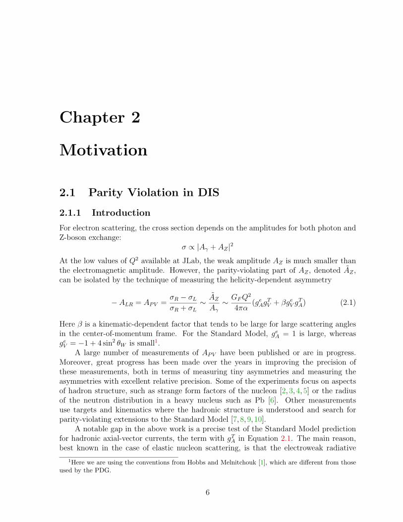
For electron scattering, the cross section depends on the amplitudes for both photon andZ-boson exchange:
σ ∝ |Aγ + AZ |2
At the low values of Q2 available at JLab, the weak amplitude AZ is much smaller thanthe electromagnetic amplitude. However, the parity-violating part of AZ , denoted AZ ,can be isolated by the technique of measuring the helicity-dependent asymmetry
− ALR = APV =σR − σL
σR + σL
∼ AZ
Aγ
∼ GFQ2
4πα(ge
AgTV + βge
V gTA) (2.1)
Here β is a kinematic-dependent factor that tends to be large for large scattering anglesin the center-of-momentum frame. For the Standard Model, ge
A = 1 is large, whereasge
V = −1 + 4 sin2 θW is small1.A large number of measurements of APV have been published or are in progress.
Moreover, great progress has been made over the years in improving the precision ofthese measurements, both in terms of measuring tiny asymmetries and measuring theasymmetries with excellent relative precision. Some of the experiments focus on aspectsof hadron structure, such as strange form factors of the nucleon [2, 3, 4, 5] or the radiusof the neutron distribution in a heavy nucleus such as Pb [6]. Other measurementsuse targets and kinematics where the hadronic structure is understood and search forparity-violating extensions to the Standard Model [7, 8, 9, 10].
A notable gap in the above work is a precise test of the Standard Model predictionfor hadronic axial-vector currents, the term with gT
A in Equation 2.1. The main reason,best known in the case of elastic nucleon scattering, is that the electroweak radiative
1Here we are using the conventions from Hobbs and Melnitchouk [1], which are different from thoseused by the PDG.
6

CHAPTER 2. MOTIVATION 7
corrections often have large uncertainties involving anapole moments or box diagramscontaining more than one quark [11,12]. Thus a precise measurement, even at the appro-priate kinematics, would be dominated by theoretical errors. The one exception is deepinelastic scattering (DIS). Since in this case the scattering is from isolated elementaryquarks, all radiative corrections are calculable.
With the advent of the 11 GeV upgrade, significant phase space for DIS measure-ments becomes available. In addition to being sensitive to axial hadronic currents, DIShas a number of other attractive features:
1. The cross sections are large.
2. Backgrounds are manageable.
3. Large values of Q2 imply large asymmetries, on the order of 10−3.
4. Precision beam polarimetry is easier with high beam energy.
Given these advantages, we believe that with the apparatus that we are proposing, wecan measure APV with a relative precision of ∼ 0.5%. This will improve the presentlimits on the axial-vector hadronic currents by about a factor of 20.
In light of the high proposed precision, we have comprehensively investigated hadroniccorrections that might be significant. The corrections are smallest for isoscalar targetslike deuterium. Even in deuterium, however, we have found two interesting effects:
1. Charge symmetry violation (CSV) at the quark level. Present limits on the as-sumption that the up quark distribution in the proton is the same as the downquark distribution in the neutron are not sufficient for our proposed precision.
2. Finite Q2 effects. Such effects are significant in the cross sections for x > 0.5, butit is not known whether or not they cancel in the asymmetry. If they do not cancel,they provide direct evidence for quark-quark correlations in the nucleon.
We find that these hadronic effects are extremely interesting in themselves.In order to untangle the hadronic and electroweak effects, we need to make precise
measurements over as large a kinematic range as possible, changing Q2, x, and y. Theimplementation of this program requires a high acceptance spectrometer that must op-erate at scattering angles on the order of 30. In this proposal we present plans to buildsuch a device.
2.1.2 PVDIS in the QPM
At JLab energies, the interactions of the Z-boson and heavier particles can be approx-imated by four-fermion contact interactions. The parity-violating part of the electron-hadron interaction can then be given in terms of phenomenological couplings Cij
LPV =GF√
2[eγµγ5e(C1uuγµu+ C1ddγµd) + eγµe(C2uuγµγ5u+ C2ddγµγ5d)]
CHAPTER 2. MOTIVATION 8
with additional terms as required for the heavy quarks. Here C1j (C2j) gives the vector(axial-vector) coupling to the jth quark. For the Standard Model,
C1u = geAg
uV ≈ − 1
2+
4
3sin2 θW ≈ − 0.19 (2.2)
C1d = geAg
dV ≈ 1
2− 2
3sin2 θW ≈ 0.34 (2.3)
C2u = geV g
uA ≈ − 1
2+ 2 sin2 θW ≈ − 0.030 (2.4)
C2d = geV g
dA ≈
1
2− 2 sin2 θW ≈ 0.025 (2.5)
Here we have used the conventions that geA = 1, ge
V = −1 + 4 sin2 θW , guA = 1/2, and
guV = −1/2 + (4/3) sin2 θW , etc. The numerical values include electroweak radiative
corrections explained in Section 5.2.2.The cross sections for DIS can be expressed in terms of structure functions F j
i (x,Q2),as discussed in detail in Appendix A.1. Here x = Q2/2Mν is the Bjorken scaling variablewith M the nucleon mass. For the spinless case, there are two electromagnetic structurefunctions, F γ
1 and F γ2 . For PVDIS, three more structure functions are involved, F γZ
1 , F γZ2
and F γZ3 . The axial-vector hadronic current is described by F γZ
3 . The relative weightingof the different structure functions is a function of the kinematic variable y ≡ ν/E, whereν is the energy loss in the lab frame.
In the limit of large Q2, the structure functions can be described by parton dis-tribution functions (PDFs) fi(x) (f i(x)), which are the probabilities that the ith quark(antiquark) carries a fraction x of the nucleon momentum. In this limit, the structurefunctions have a logarithmic Q2-dependence given by QCD evolution. With the defini-tions f±i = fi ± f i, y = ν/E, the asymmetry can be written
APV = − GFQ2
4√
2πα[Y1a1(x) + Y3(y)a3(x)] (2.6)
where
Y1 ≈ 1; Y3 ≈1− (1− y)2
1 + (1− y)2≡ f(y) (2.7)
and
a1(x) = geA
F γZ1
F γ1
= 2
∑iC1iQif
+i (x)∑
iQ2i f
+i (x)
; a3(x) =ge
V
2
F γZ3
F γ1
= 2
∑iC2iQif
−i (x)∑
iQ2i f
+i (x)
For isoscalar targets such as the deuteron, the structure functions cancel and we have
aD1 (x) =
6
5(2C1u−C1d)
(1 +
0.6s+
u+ + d+
); aD
3 (x) =6
5(2C2u−C2d)
(u− + d−
u+ + d+
)+ . . . (2.8)
For x > 0.4, only valence quarks are important, and the expressions for a1 and a3 becomeconstants. Then the asymmetry becomes
ADPV = −GFQ
2
√2πα
(9
20
) [1− 20
9sin2 θW + (1− 4 sin2 θW )f(y)
]. (2.9)
CHAPTER 2. MOTIVATION 9
2.1.3 Additional Corrections
A detailed study of the above phenomenology [1] reveals additional corrections that willbe important at our level of precision. First, the approximation that r2 in Equation A.2is unity. That and similar terms in Appendix A.1 make about a 0.5% correction forQ2=5 GeV2.
A more interesting observation is that the Y1 term depends on y. We have
limy→0
Y1 =
(1 +RγZ
1 +Rγ
); lim
y→1Y1 ≈ 1
where the second limit neglects the 2xyM/E term in Equation A.4.Another important effect is target mass corrections. We anticipate that there will
be substantial cancellation in the ratio APV as is the case for spin-dependent structurefunctions [13].
2.2 Electroweak Physics
0.001 0.01 0.1 1 10 100 1000 [GeV]
0.225
0.230
0.235
0.240
0.245
0.250
sin2 θ
W^ APV(Cs)
Qweak [JLab]
Moller [SLAC]
ν-DIS
ALR(had) [SLC]AFB(b) [LEP]
AFB(lep) [Tevatron]
screening
antis
cree
ning
Moller [JLab]
PV-DIS [JLab]
SMcurrentfuture
μ
(μ)
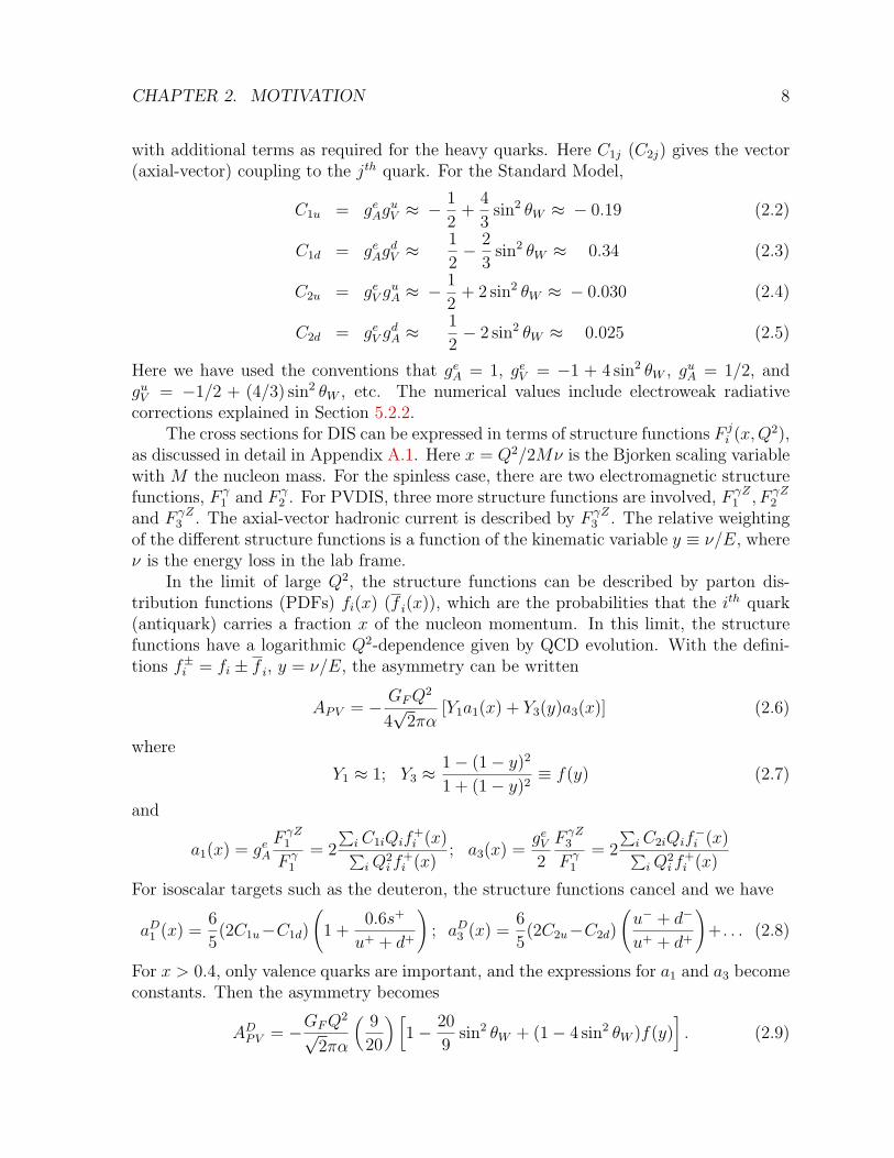
Figure 2.1: Plot of sin2 θW versus Q for various precision experiments that are eithercompleted or proposed.
One goal of PVDIS is to search for new physics beyond the Standard Model. Withthat in mind, we have designed the experiment so that we can obtain a precision of

CHAPTER 2. MOTIVATION 10
0.6% on the combination of electroweak parameters in ADPV , as described in Section 2.4.3
below. One signature for the new physics is a deviation of the value of sin2 θW obtainedfrom comparing the data with Equation 2.9. The resulting sensitivity for our projectederror is plotted in Figure 2.1, together with the results of other precise measurements,both published and proposed.
0.05
0.1
0.15
0.2
0.25
0.3
-0.65 -0.6 -0.55 -0.5 -0.45 -0.4C1u-C1d
C1u
+C
1d
-0.15
-0.1
-0.05
0
0.05
0.1
-0.2 -0.15 -0.1 -0.05 0 0.05C2u-C2d
C2u
+C
2d
Figure 2.2: Constraints on the Standard Model from parity-violation experiments. Themagenta/yellow hatched bands present the SLAC-DIS/Bates results. The cyan/blackhatched band presents the Tl/Cs APV result. The narrow black band in the left plotshows the expected results from Qweak. The red band in the right plot shows the PDGconstraint, and the blue band shows the expected precision from the approved 6 GeVPVDIS experiment (E08-011) [14] which will run in 2009. The green bands show theexpected results from the experiment proposed. All limits are 1 standard deviation.
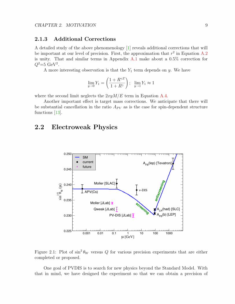
From a more phenomenological perspective, a measurement of ADPV provides a limit
on deviations of the couplings Cij from the predictions of the Standard Model. Theresulting sensitivity on plots of the Cij’s is given in Figures 2.2 and 2.3. There is atremendous decrease in the allowed region of the C2 plot. Both the high statisticalsensitivity and the large values of Y3 due to the large scattering angles are important forthis improvement. The unique feature of PVDIS is that it provides a precise constraintin the plot of the C2’s.
As discussed in a recent review by Ramsey-Musolf and Su [15], combining vari-ous precision measurements at low energies can have an important impact on physicsbeyond the Standard Model. In this spirit, these data will be complementary to theanticipated high-energy data from the LHC. PVDIS is one example of these low-energyexperiments [16].
CHAPTER 2. MOTIVATION 11
0.14
0.145
0.15
0.155
0.16
0.165
-0.53 -0.525 -0.52 -0.515 -0.51 -0.505C1u-C1d
C1u
+C
1d
-0.02
-0.015
-0.01
-0.005
0
0.005
-0.075 -0.07 -0.065 -0.06 -0.055 -0.05C2u-C2d
C2u
+C
2d
Figure 2.3: Expanded view of constraints on the Standard Model from parity-violationexperiments (Fig. 2.2). The black crossed band presents the Cs APV results, the blueband - the expected QWEAK result, the red ellipse is a PDG fit, the black dots indicatethe SM expectation and the best PDG fit, while the green band shows the currentproposal. The anticipated error band from the future E08-011 experiment would also fillthe entire region visible in the right plot. All limits are 1 standard deviation.
2.2.1 Contact Interactions
A general, model-independent way to parametrize the contributions of contact interac-tions of high-mass particles to low-energy measurements is to use the Lagrangian
Leq =∑
i,j=L,R
g2ij
Λ2eiγµei qjγ
µqj (2.10)
Here eL/R = 12(1 ∓ γ5)ψe and qL/R = 1
2(1 ∓ γ5)ψq are the chirality projections of the
fermion spinors, the gij are the coupling constants gij = 2guij − gd
ij and Λ is the massscale.
The projected results on ADPV translates into a measurement of the linear com-
bination of the phenomenological couplings 2 [(2C1u − C1d)− 0.84 (2C2u − C2d)] to anaccuracy of ±0.0098. This translates into
Λ√|g2
RR − g2LL + g2
RL − g2LR|
=1√√
2GF |0.0098|' 2.5 TeV. (2.11)
For example, models of lepton compositeness are characterized by strong coupling dy-
namics. Taking√|g2
RR − g2LL + g2
RL − g2LR| = 2π shows that mass scales as large as
Λ = 15.5 TeV can be probed, corresponding to electron and quark substructure at thelevel of ∼ 10−20 m.
CHAPTER 2. MOTIVATION 12
There are two kinds of new interactions that can contribute to PVDIS. One is thecontact interactions mentioned above, which can include particles such as extra Z-bosons,leptoquarks, and supersymmetric (SUSY) partners. Contact interactions have real am-plitudes, so they do not interfere with the imaginary amplitudes measured on the Z-poleat LEP and SLAC. Hence low energy measurements are competitive. In addition, the newgeneration of experiments at JLab, including Qweak, PVDIS, and Møller, has the pre-cision to probe contributions to radiative corrections from loops involving new particlesthat do not directly couple to quarks and leptons.
2.2.2 Z ′ Bosons
A specific example of the kind of new physics to which the proposed experiment may besensitive to are extra neutral gauge (Z ′) bosons with masses, MZ′ , in the TeV region.While these are very well motivated in many (if not most) models of physics beyond theSM, they are in general severely constrained by atomic parity violation (APV) measure-ments in Cs (and Tl) which agree with the SM prediction. However, APV in heavy nucleiis sensitive roughly to the sum of up and down quark vector couplings, and is thus blindto models where these are of similar size but opposite sign.
An example is the case where only right-handed quarks and leptons are chargedunder the underlying extra U(1)′ gauge factor2 with charges proportional to the thirdcomponent of the SU(2)R gauge group appearing in left-right symmetric models (it isnot actually necessary that the U(1)′ is promoted to SU(2)R). This case is interestingsince the current precision electroweak data can accommodate such a heavy Z ′ with amass as small as 660 GeV. If this case was actually realized in nature, the proposedmeasurement would see a 4σ deviation from the Standard Model prediction. For thisparticular example, the senstivity of this proposal exceeds that of any other low-energyparity-violation measurement in the electron-quark sector.
2.2.3 Supersymmetry
Another good example of new physics contributing to APV is in the case of SUSY.Predictions for the contributions of SUSY to both PVDIS and Qweak for models ofsupersymmetry (SUSY) are shown in Fig. 2.4. There are two classes of models shown, onethat conserves R-parity and one that does not. For R-parity conserving models, where theeffects are confined to loops, PVDIS is a bit more sensitive, but the predictions are highlycorrelated. For the R-parity-violating case, where contact interactions are important, thepredictions for the two experiments are totally uncorrelated. If SUSY were observed atthe LHC and the result from PVDIS were below the prediction, the implication wouldbe that SUSY violates R-parity, which in turn implies that the lightest SUSY particle isunstable and is not a good candidate for dark matter.
2For instance, a model of this type can be obtained from an E6 gauge group when large kinetic mixingwith the hypercharge boson is induced.

CHAPTER 2. MOTIVATION 13
!!" !!# !" # " !# !"!$
!!%"
!!
!#%"
#
#%"
!
!&'()
*+,-,.
/'()
*+,0&&'1+
!&'23+ ,-,./&'23+ ,0&&&&'1+
'4+
Figure 2.4: Implications of a measurement of PVDIS and Qweak for SUSY models.Dots: typical models for the R-parity conserving case. Line: region allowed at the 95%confidence level for models that violate R-parity but are consistent with other existingelectroweak data.
2.3 Hadron Physics with Deuterium
2.3.1 Charge Symmetry Violation
One critical assumption for the cancellation of the structure functions in APV for thedeuteron is charge symmetry, namely up = dn and un = dp. Charge symmetry violation(CSV) can be parametrized by new PDFs
δu ≡ up − dn; δd ≡ dp − un; RCSV ≡ δu− δd
u+ v
Although the δu and δd are small, the ratio RCSV can be significant if these CSV PDFsdrop more slowly than the valence u and d with increasing x. There is no direct evidencefor CSV at the parton level [17]. However, our PVDIS data will be more sensitive toCSV than any previous data, so we can set the best limits at large values of x.
There is some indirect evidence for CSV in neutrino scattering [18,19]. The Paschos-Wolfenstein ratio
RPW =σ〈νN → νX〉 − σ〈νN → νX〉σ〈νN → µX〉 − σ〈νN → µX〉
∼ 1
2− sin2 θW
which has been precisely measured by the NuTeV collaboration [20], is quite sensitive toCSV. In particular,
δRPW
RPW∼ 0.85RCSV

CHAPTER 2. MOTIVATION 14
bjx0.2 0.4 0.6 0.8
CSV
R
−0.04
−0.02
0.00
BAG Model + QED SplittingQED Splitting in MRSTUncertainty band, this proposal
δAPVAPV
Figure 2.5: CSV predictions as a function of x. The vertical axis is the fractional changein APV due to CSV. The uncertainty band is the result of the fit discussed in Section 2.4.2.The MRST results shown here account for QED splitting in the Q2 evolution only, anddo not include non-pertubative QCD effects [24].
The discrepancy of the NuTeV result with the Standard Model expectation may indeedbe due to CSV.
As a consequence of the above, the MRST group inserted CSV-violating terms totheir global fits [21] and found that sufficient CSV is allowed to account for the NuTeVresult. Non-zero values of RCSV have been suggested in the literature caused both bynon-perturbative QCD effects [22,23] as well as QED effects in the Q2 evolution [24,25].These are also in the range that would be significant for the NuTeV result.
The corrections due to CSV for APV for deuterium are
δCSV aD1
ad1
=
(3
10+
2C1u + C1d
2(2C1u − C1d
)RCSV
δCSV aD3
ad3
=
(3
10+
2C2u + C2d
2(2C2u − C2d)
)RCSV
The effect of the CSV suggested in Ref. [22, 23, 24, 25] on APV is plotted in Figure 2.5.The size of the CSV effect is within reach of our sensitivity.
Since we can obtain high precision in several narrow bins of x for x > 0.4 with theJLab upgrade, we will be in an ideal position to study CSV. In contrast to physics beyondthe Standard Model, the effect depends strongly on x. This signature will be a powerfulmethod for discriminating CSV from new physics as an explanation for any deviationfrom the prediction of Equation 2.8.

CHAPTER 2. MOTIVATION 15
Although the Paschos-Wolfenstein ratio is more sensitive to RCSV , neutrino experi-ments to date have not been able to obtain high statistics on small bins in the relevantkinematic range. Another approach to studying CSV is to measure asymmetries in W-production at colliders, but the experimental sensitivity is not very good [26]. Otherpossible CSV experiments include pion-induced Drell-Yan scattering and pion electro-production sum rules [27,28], but these approaches have complications such as fragmen-tation functions and CSV in sea quarks.
2.3.2 Higher Twist Effects in DIS
A remarkable feature of DIS behavior is that higher twist effects for data where themass of the final state W > 2 GeV are found to be small. For example, the highertwist terms have been determined recently for the measured e-p DIS structure functionsF2(x,Q
2) [21] after the DGLAP evolution is removed. The ansatz is
F γ2 (x,Q2) = F γ
2 (x)(1 +D(x)/Q2)
It turns out that the values of the D(x) depend upon how many orders of αs are taken inthe DGLAP evolution of the PDFs. At leading order (LO), the higher twist contributionsare significant and similar to the results of older analysis [29, 30]. However, as higherorders are taken, NLO, NNLO, and NNNLO, D(x) becomes quite small, especially forx < 0.4. The values of Di for both LO and NNNLO are summarized in Table 2.1.Recently the work on higher twists has been extended to one more order [31].
To interpret the size of higher twist terms at large values of x, one must take intoaccount the relationship between W , Q2 and x:
Q2 = (W 2 −M2)/(1/x− 1).
If W = 2 GeV is taken as the threshold for DIS behavior, then there is a threshold Q2
denoted Q2t . Values for Q2
t are also given in Table 2.1. The maximum size of the highertwist effect that can be measured is thus D(x)/Q2
t , which is also given in Table 2.1 as afraction of F γ
2 (x). This fraction is large enough to motivate a measurement only at highx.
We can include higher twist terms in a1(x) by defining
a1(x,Q2) = a1(x)(1 + C(x)/Q2).
As described in the next section, it is only quark-quark correlation that contributes toC(x), whereas many possible higher-twist operators might contribute to D(x). Hence itis plausible that C(x) ≤ D(x). Based on this assumption and Table 2.1, higher twisteffects in C(x) are probably impractical to isolate in PV DIS for x < 0.4. However, for0.5 < x < 0.7, it is possible that these effects could be observed cleanly. Moreover, sincethe effects of the DGLAP evolution cancel in the ratio aD
1 (x), there is no problem withthe order to which the evolution is performed.

CHAPTER 2. MOTIVATION 16
Table 2.1: Higher twist coefficients D(x) from Ref. [21].
x D(x) D(x) Q2t D(x)/Q2
t D(x)/Q2t
(%) (%)(LO) (N3LO) (LO) (N3LO)
0.15 -0.07 0.01 0.5 -14 0.20.25 -0.11 0.00 1.0 -11 00.35 -0.06 -0.01 1.7 -3.5 -0.0590.45 0.22 .11 2.6 8 40.55 0.85 0.39 3.8 22 100.65 2.6 1.4 5.8 45 240.75 7.3 4.4 9.4 78 47
2.3.3 Q2 Dependence and Quark-Quark Correlations
The term Y1aD1 involves only conserved vector currents. As a consequence, we can make a
strong statement about possible hadronic corrections that were addressed by Bjorken [32],Wolfenstein [33], and Derman [34] shortly after the data of Prescott, et al. were published.Going back to the hadronic tensor in terms of currents, we can write aD
i as
Y1aD1 ∝
Lµνγ
∑X〈X|JZV
µ |〉∗〈X|Jγν |D〉+H.C.(2π)3δ(PX − p− q)
Lµνγ∑
X〈X|Jγµ |〉∗〈X|Jγ
ν |D〉+H.C.(2π)3δ(PX − p− q)
where JZV is the vector part of the weak current. Next, we decompose the vector currentsin terms of isospin
Vµ = (uγµu− dγµd); Sµ = (uγµu+ dγµd)
and define〈V V 〉 = Lµν
γ
∑X
〈X|Vµ|D〉∗〈X|Vν |D〉(2π)3δ(PX − p− q)
with similar expressions for 〈SS〉 and 〈SV 〉Then the asymmetry is proportional to
Y1aD1 ∝
(C1u − C1d)〈V V 〉+ 13(C1u + C1d)〈SS〉
〈V V 〉+ 13〈SS〉
(2.12)
The key here is that the 〈SV 〉 term vanishes in the absence of CSV. Strange quarks havealso been neglected. If 〈V V 〉 = 〈SS〉, the hadronic structure completely cancels. Thedifference between 〈V V 〉 and 〈SS〉 can be written
〈V V 〉 − 〈SS〉 = 〈(V − S)(V + S)〉 ∝
Lµνγ
∑X
〈X|uγµu|D〉∗〈X|dγνd|D〉+H.C.(2π)3δ(PX − p− q) (2.13)

CHAPTER 2. MOTIVATION 17
If this expression vanishes, all of the hadronic structure in Equation 2.12 cancels andthe Y1a
D1 part of the asymmetry is strictly independent of Q2. The right hand side of
Equation 2.13 is a correlation between u and d quarks. Thus any Q2 dependence observedin this term will be a measure of quark correlations. The only assumption is that thehadronic vector current is conserved (CVC).
The valence PDFs drop rapidly after x ∼ 0.3. However, the x relevant to the quark-quark correlation function is the sum of the individual x-values of each quark, so it islikely that the correlation function doesn’t fall rapidly until x ∼ 0.6 or so. Thus the ratioof diquarks to single quarks may be strongly enhanced at large x. This argument suggeststhat the x-dependence of the diquarks could be similar to the observed x-dependence ofthe higher twist coefficients C(x).
Based on the above ideas, one method to remove the contribution of higher twistterms is to do a global fit of the form D(X) = α(1−x)−n, where α and n are parametersto be fit. If little Q2-dependence is observed, tight bounds on the amplitudes will befound for n > 2. In this scenario, the contribution of the uncertainties in the higher twistcoefficient to the high Q2 point at x ∼ 0.4 would be small.
In summary, the observation of Q2-dependent effects would be of particular inter-est [35] in PVDIS because:
1. The experimental signature is especially clean. It is a violation of the QPM pre-diction that varies with both Q2 and x. Since the DGLAP evolution cancels in theratio, there is no uncertainty associated with the order to which the evolution isperformed.
2. The theoretical interpretation, namely quark correlations, is well defined and in-teresting.
2.3.4 Higher Twist and the Operator Product Expansion
Estimates of the size of higher twist effects that use the operator product expansion(OPE) in QCD have been made by Castorina and Mulders [36] and Fajfer and Oakes [37].These papers are based on the OPE analysis of Jaffe and Soldate [38], in which the twist-4 (∼ 1/Q2) contributions are expressed in terms of a set of symmetric, traceless, andderivative-free operators. The QCD equations of motion are used to eliminate thoseoperators that arise that do not satisfy these conditions. Such operators are a startingpoint for a rigorous phenomenology of higher twist effects. The computation of thematrix elements of these operators is presently less rigorous, and the MIT bag model hasbeen used to make rough estimates.
For their analysis, Castorina and Mulders use a slightly different expression for theasymmetry
A
Q2= a1 + a2f(y) + a3g(y) + a4f(y)g(y)
CHAPTER 2. MOTIVATION 18
where
f(y) =1− (1− y)2
1 + (1− y)2; g(y) =
y2
1 + (1− y)2
and
a1 = − GF
4√
2πα
F γZ2
F γ2
a2 = − GF
4√
2πα(1− 4 sin2 θW )
xF γZ3
F γ2
a3 = − GF
4√
2πα
[2xF γ
LFγZ2
(F γ2 )2
− 2xF γZL
F γ2
]
a4 = − GF
4√
2πα(1− 4 sin2 θW )
2xF γLxF
γZ3
(F γ2 )2
where the approximation
1
F2 − g(y)2xFL
≈ 1
F2
(1 +
g(y)2xFL
F2
)
is used and F2 is used as the denominator instead of F1 as is done in the appendix.The higher twist contributions are given in terms of constants K1 and K2 computed
in the MIT bag model;
a1 = − GF
4√
2πα
9
4
[1 +
1
Q2(−1.4K1 + 3.8K2)−
20
9sin2 θW
]
a2 = − GF
4√
2πα
9
4
[1 +
1
Q2(11.5K1 − 23.5K2)
](1− 4 sin2 θW )
a3 = 0
a4 =GF
4√
2πα
9
4
[1
Q2(4K1 − 3.5K2)
](1− 4 sin2 θW )
The most striking result is that a3 = 0. As stated in the paper, this feature arisesbecause the breaking of the Callan-Gross relation (FL = 0) is due to two-quark-gluonoperators, which contribute to the γ and γZ terms proportional to the leading twist-2results. Therefore, there is no contribution to the ratio. This is consistent with theargument due to Bjorken that the only higher twist operators in a1 involve quark-quarkcorrelations, which are four-quark operators. This result of the calculation is expectedto be quite general in the context of QCD.
The analysis of Castorina and Mulders only considered one moment of the highertwist contributions, so it applies only to the average over all x-values. It is quite likely,however, that the effects are larger at larger x. From a theoretical standpoint, the quark-quark correlations add the x-values of each quark, resulting in relatively greater strength
CHAPTER 2. MOTIVATION 19
at larger x, as suggested by Brodsky [35]. From an empirical standpoint, the higher twistcontribution to F γ
2 is observed to be significant only at large x as discussed in Sec. 2.3.2.The higher twist contribution to the electromagnetic structure function
F γ2 → F γ
2
[1 +
1
Q2(17.4K1 − 29K2)
]
is much larger than the contribution to a1. It is not clear if this is an artifact of the MITbag model and other approximations or a more general feature in QCD. The higher twisteffects in the a2 term are larger. However, the higher twist in the F3 structure functionsobserved in neutrino scattering [39] have strength at moderate x, in sharp contrast tothe electro-production data. It is possible that future theoretical work might shed lighton these and other similar issues.
2.3.5 Physics of Y3aD3 (x)
For the contribution to APV due to F γZ3 , there is no CVC theorem to help cancel uncer-
tainties in the structure functions in the asymmetry. Fortunately, the a3(x) term is smallin the Standard Model
a3(x)
a1(x)∼ 11.5%
so a precision of only about 5% is required. The suppression factor is essentially the ratioof electron-Z couplings ge
V /geA.
In the QPM, the structure functions cancel if the sea quarks are negligible. Basedon experiments of muon pair production by the Drell-Yan mechanism, sea quarks areknown to be negligible at large x. The remaining problem is the dependence of Rγ inthe Y3 factor. Since Rγ is known from data [40] with an uncertainty of about 0.05, theuncertainty in Y3a
D3 contributes about 0.5% to APV .
Another approach is to note that the axial current is just an isospin rotation of theν −D charge current interaction
F γZ3 ∝ F ν
3 − F ν3
Thus data [41] can be used to determine F γZ3 /F γ
2 . Since
limy→0
Y3aD3 = y
F γZ3
F γ2
; limy→1
Y3aD3 =
F γZ3
F γ1
= C2u − C2d
where the second equality arises from the absence of sea quarks at large x in the QPM.Finally, Y3a
D3 for arbitrary y is a weighted sum of the above two limits. This procedure
also has an acceptable uncertainty.
CHAPTER 2. MOTIVATION 20
bjx0.2 0.4 0.6 0.8
2Q
5
10
0.570.51
0.500.550.50
0.50 0.47
0.520.52
0.53
0.65
0.58
0.67
0.61 0.63
2.810.74
0.470.38
0.370.40 0.45 0.51
0.89
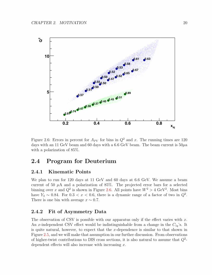
Figure 2.6: Errors in percent for APV for bins in Q2 and x. The running times are 120days with an 11 GeV beam and 60 days with a 6.6 GeV beam. The beam current is 50µawith a polarization of 85%.
2.4 Program for Deuterium
2.4.1 Kinematic Points
We plan to run for 120 days at 11 GeV and 60 days at 6.6 GeV. We assume a beamcurrent of 50 µA and a polarization of 85%. The projected error bars for a selectedbinning over x and Q2 is shown in Figure 2.6. All points have W 2 > 4 GeV2. Most binshave Y3 ∼ 0.84. For 0.3 < x < 0.6, there is a dynamic range of a factor of two in Q2.There is one bin with average x ∼ 0.7.
2.4.2 Fit of Asymmetry Data
The observation of CSV is possible with our apparatus only if the effect varies with x.An x-independent CSV effect would be indistinguishable from a change in the C1q’s. Itis quite natural, however, to expect that the x-dependence is similar to that shown inFigure 2.5, and we will make that assumption in our further discussion. From observationsof higher-twist contributions to DIS cross sections, it is also natural to assume that Q2-dependent effects will also increase with increasing x.
CHAPTER 2. MOTIVATION 21
bjx0.2 0.4 0.6 0.8
HT
D
0
2
4Higher Twist Coefficients D(x)HT Fit 1/(1−x)^3Uncertainty band, this proposal
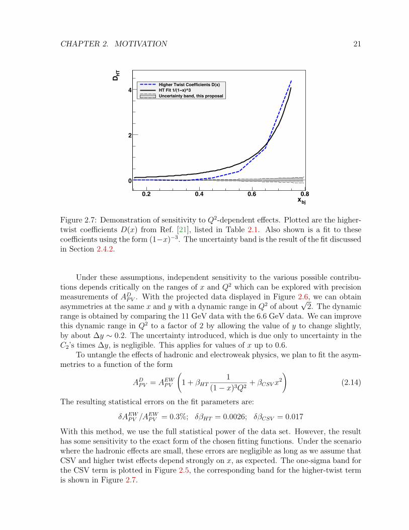
Figure 2.7: Demonstration of sensitivity to Q2-dependent effects. Plotted are the higher-twist coefficients D(x) from Ref. [21], listed in Table 2.1. Also shown is a fit to thesecoefficients using the form (1−x)−3. The uncertainty band is the result of the fit discussedin Section 2.4.2.
Under these assumptions, independent sensitivity to the various possible contribu-tions depends critically on the ranges of x and Q2 which can be explored with precisionmeasurements of AD
PV . With the projected data displayed in Figure 2.6, we can obtainasymmetries at the same x and y with a dynamic range in Q2 of about
√2. The dynamic
range is obtained by comparing the 11 GeV data with the 6.6 GeV data. We can improvethis dynamic range in Q2 to a factor of 2 by allowing the value of y to change slightly,by about ∆y ∼ 0.2. The uncertainty introduced, which is due only to uncertainty in theC2’s times ∆y, is negligible. This applies for values of x up to 0.6.
To untangle the effects of hadronic and electroweak physics, we plan to fit the asym-metries to a function of the form
ADPV = AEW
PV
(1 + βHT
1
(1− x)3Q2+ βCSV x
2
)(2.14)
The resulting statistical errors on the fit parameters are:
δAEWPV /A
EWPV = 0.3%; δβHT = 0.0026; δβCSV = 0.017
With this method, we use the full statistical power of the data set. However, the resulthas some sensitivity to the exact form of the chosen fitting functions. Under the scenariowhere the hadronic effects are small, these errors are negligible as long as we assume thatCSV and higher twist effects depend strongly on x, as expected. The one-sigma band forthe CSV term is plotted in Figure 2.5, the corresponding band for the higher-twist termis shown in Figure 2.7.
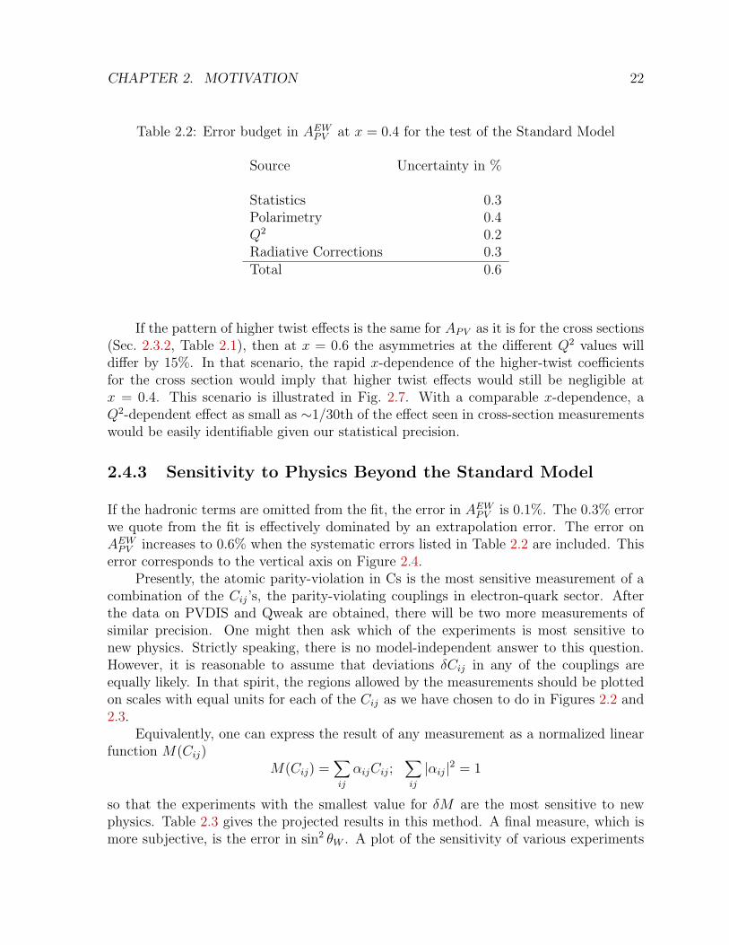
CHAPTER 2. MOTIVATION 22
Table 2.2: Error budget in AEWPV at x = 0.4 for the test of the Standard Model
Source Uncertainty in %
Statistics 0.3Polarimetry 0.4Q2 0.2Radiative Corrections 0.3Total 0.6
If the pattern of higher twist effects is the same for APV as it is for the cross sections(Sec. 2.3.2, Table 2.1), then at x = 0.6 the asymmetries at the different Q2 values willdiffer by 15%. In that scenario, the rapid x-dependence of the higher-twist coefficientsfor the cross section would imply that higher twist effects would still be negligible atx = 0.4. This scenario is illustrated in Fig. 2.7. With a comparable x-dependence, aQ2-dependent effect as small as ∼1/30th of the effect seen in cross-section measurementswould be easily identifiable given our statistical precision.
2.4.3 Sensitivity to Physics Beyond the Standard Model
If the hadronic terms are omitted from the fit, the error in AEWPV is 0.1%. The 0.3% error
we quote from the fit is effectively dominated by an extrapolation error. The error onAEW
PV increases to 0.6% when the systematic errors listed in Table 2.2 are included. Thiserror corresponds to the vertical axis on Figure 2.4.
Presently, the atomic parity-violation in Cs is the most sensitive measurement of acombination of the Cij’s, the parity-violating couplings in electron-quark sector. Afterthe data on PVDIS and Qweak are obtained, there will be two more measurements ofsimilar precision. One might then ask which of the experiments is most sensitive tonew physics. Strictly speaking, there is no model-independent answer to this question.However, it is reasonable to assume that deviations δCij in any of the couplings areequally likely. In that spirit, the regions allowed by the measurements should be plottedon scales with equal units for each of the Cij as we have chosen to do in Figures 2.2 and2.3.
Equivalently, one can express the result of any measurement as a normalized linearfunction M(Cij)
M(Cij) =∑ij
αijCij;∑ij
|αij|2 = 1
so that the experiments with the smallest value for δM are the most sensitive to newphysics. Table 2.3 gives the projected results in this method. A final measure, which ismore subjective, is the error in sin2 θW . A plot of the sensitivity of various experiments
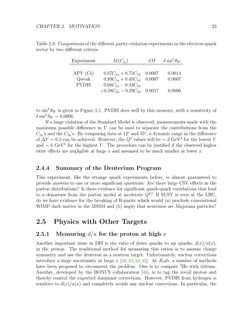
CHAPTER 2. MOTIVATION 23
Table 2.3: Comparisons of the different parity-violation experiments in the electron-quarksector by two different criteria
Experiment M(Cij) δM δ sin2 θW
APV (Cs) 0.67C1u + 0.75C1d 0.0007 0.0014Qweak 0.89C1u + 0.45C1d 0.0007 0.0007PVDIS 0.68C1u − 0.34C1d
+0.58C2u − 0.29C2d 0.0017 0.0006
to sin2 θW is given in Figure 2.1. PVDIS does well by this measure, with a sensitivity ofδ sin2 θW = 0.0006.
If a large violation of the Standard Model is observed, measurements made with themaximum possible difference in Y can be used to separate the contributions from theC1q’s and the C2q’s. By comparing data at 12 and 35, a dynamic range in the differenceof ∆Y ∼ 0.5 can be achieved. However, the Q2 values will be ∼ 3 GeV2 for the lowest Yand ∼ 6 GeV2 for the highest Y . The procedure can be justified if the observed highertwist effects are negligible at large x and assumed to be much smaller at lower x.
2.4.4 Summary of the Deuterium Program
This experiment, like the strange quark experiments before, is almost guaranteed toprovide answers to one or more significant questions: Are there large CSV effects in theparton distributions? Is there evidence for significant quark-quark correlations that leadto a departure from the parton model at moderate Q2? If SUSY is seen at the LHC,do we have evidence for the breaking of R-parity which would (a) preclude conventionalWIMP dark matter in the MSSM and (b) imply that neutrinos are Majorana particles?
2.5 Physics with Other Targets
2.5.1 Measuring d/u for the proton at high x
Another important issue in DIS is the ratio of down quarks to up quarks, d(x)/u(x),in the proton. The traditional method for measuring this ration is to assume chargesymmetry and use the deuteron as a neutron target. Unfortunately, nuclear correctionsintroduce a large uncertainty at large x [42, 43, 44, 45]. At JLab, a number of methodshave been proposed to circumvent the problem. One is to compare 3He with tritium.Another, developed by the BONUS collaboration [46], is to tag the recoil proton andthereby control the expected dominant corrections. However, PVDIS from hydrogen issensitive to d(x)/u(x) and completely avoids any nuclear corrections. In particular, the
CHAPTER 2. MOTIVATION 24
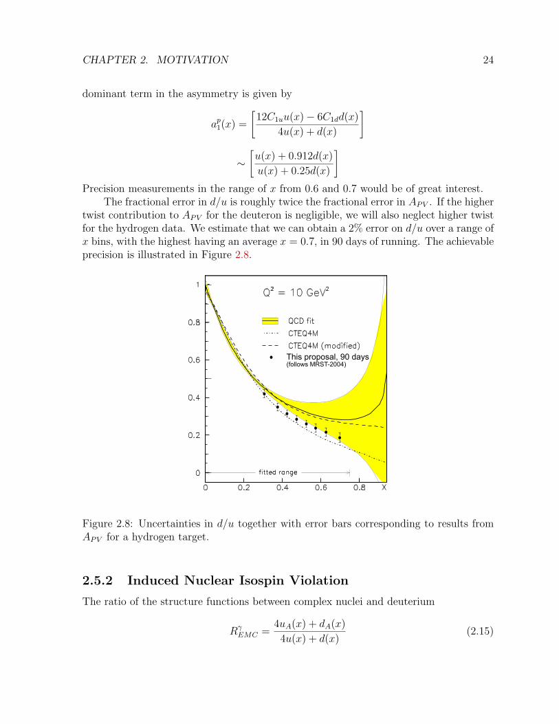
dominant term in the asymmetry is given by
ap1(x) =
[12C1uu(x)− 6C1dd(x)
4u(x) + d(x)
]
∼[u(x) + 0.912d(x)
u(x) + 0.25d(x)
]Precision measurements in the range of x from 0.6 and 0.7 would be of great interest.
The fractional error in d/u is roughly twice the fractional error in APV . If the highertwist contribution to APV for the deuteron is negligible, we will also neglect higher twistfor the hydrogen data. We estimate that we can obtain a 2% error on d/u over a range ofx bins, with the highest having an average x = 0.7, in 90 days of running. The achievableprecision is illustrated in Figure 2.8.
This proposal, 90 days(follows MRST-2004)
Figure 2.8: Uncertainties in d/u together with error bars corresponding to results fromAPV for a hydrogen target.
2.5.2 Induced Nuclear Isospin Violation
The ratio of the structure functions between complex nuclei and deuterium
RγEMC =
4uA(x) + dA(x)
4u(x) + d(x)(2.15)
CHAPTER 2. MOTIVATION 25
Q2 = 5.0 GeV 2
Carbon
0.6
0.7
0.8
0.9
1
1.1
1.2a 1
(x)
0 0.2 0.4 0.6 0.8 1x
a1a1,naive
Q2 = 5.0 GeV 2
Iron
0.8
0.9
1
1.1
1.2
a 1(x
)
0 0.2 0.4 0.6 0.8 1x
a1a1,naive
Q2 = 5.0 GeV 2
Lead
0.8
0.9
1
1.1
1.2
a 1(x
)
0 0.2 0.4 0.6 0.8 1x
a1a1,naive
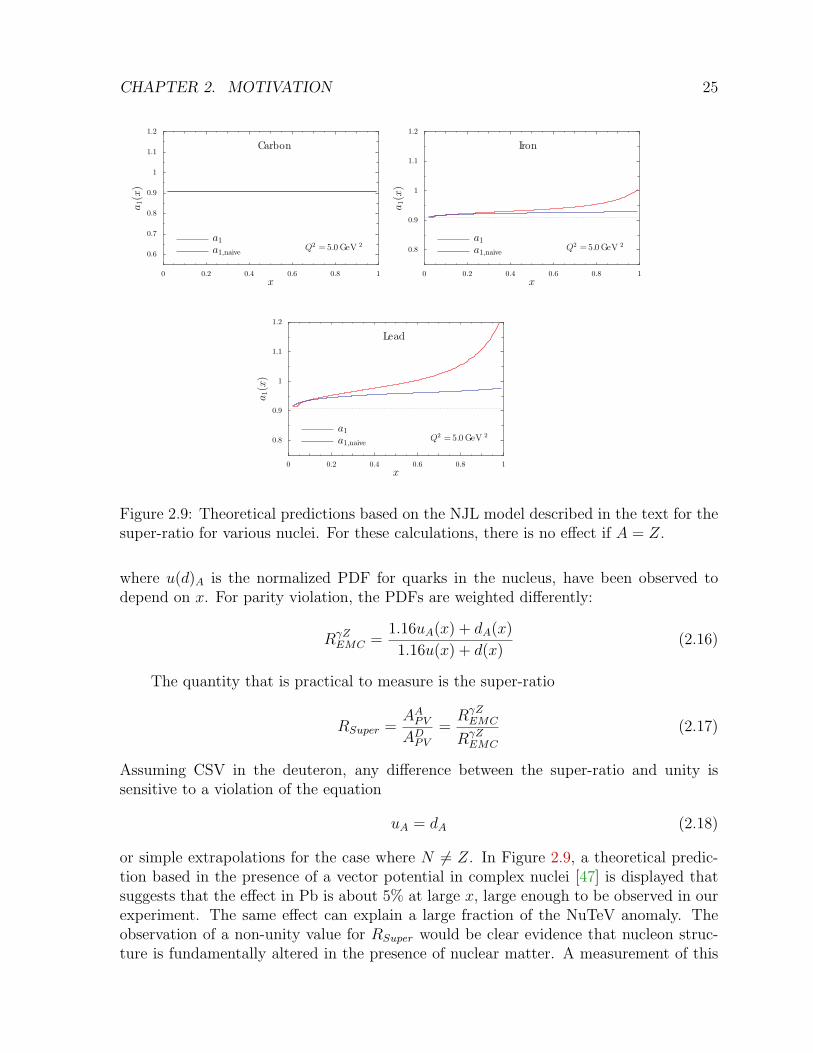
Figure 2.9: Theoretical predictions based on the NJL model described in the text for thesuper-ratio for various nuclei. For these calculations, there is no effect if A = Z.
where u(d)A is the normalized PDF for quarks in the nucleus, have been observed todepend on x. For parity violation, the PDFs are weighted differently:
RγZEMC =
1.16uA(x) + dA(x)
1.16u(x) + d(x)(2.16)
The quantity that is practical to measure is the super-ratio
RSuper =AA
PV
ADPV
=RγZ
EMC
RγZEMC
(2.17)
Assuming CSV in the deuteron, any difference between the super-ratio and unity issensitive to a violation of the equation
uA = dA (2.18)
or simple extrapolations for the case where N 6= Z. In Figure 2.9, a theoretical predic-tion based in the presence of a vector potential in complex nuclei [47] is displayed thatsuggests that the effect in Pb is about 5% at large x, large enough to be observed in ourexperiment. The same effect can explain a large fraction of the NuTeV anomaly. Theobservation of a non-unity value for RSuper would be clear evidence that nucleon struc-ture is fundamentally altered in the presence of nuclear matter. A measurement of this
CHAPTER 2. MOTIVATION 26
effect would be valuable and appears feasible in PVDIS. Although this proposal focuseson measurements with hydrogen and deuterium, this topic is mentioned as an exampleof further electroweak studies which would be enabled by the SoLID spectrometer.
Chapter 3
Large Acceptance Apparatus forHigh Luminosity
3.1 General Requirements
The main purpose of the spectrometer designed is to measure the Parity Violation effectsin DIS (PVDIS) at W > 2 GeV, Q2 > 6 GeV2 and in a wide range of xBj, namely0.3 < xBj < 0.8, with an accuracy of about 1%. Since the DIS cross section dropssharply at xBj > 0.5 the apparatus should provide a large acceptance in that area.The acceptance may be somewhat smaller at xBj < 0.5. The current design aimed tomaximize rates in the region xBj > 0.55. The useful kinematic range of the scatteredelectron is shown in Fig. 3.1. The spectrometer should accept the scattered electrons ina relatively narrow band in the E ′−θ parameter space. The acceptance in the scatteringangle θ is limited at θ > 18 by the Q2 > 6 GeV2 cut. The upper limit on θ is definedby the figure of merit of the asymmetry measurement as well as the implementationlimitations.
We assume a current of 50 µA at 11 GeV and 85% polarization, and use a 40 cmliquid hydrogen target to provide a luminosity of L ∼ 5.4 · 1038 cm−2s−1 = 540 pb−1s−1.
The asymmetry to be measured (see Eq. 2.6) is APV ∼ 0.84 · 10−4 GeV−2 ·Q2. Thefigure of merit depends on the asymmetry measured and the number of detected eventsF = A2
PV ·Nevents. The maximum occurs at θ ∼ 20 (see Fig. 3.2), while at 35 the valuedrops by a half. Typically, there are additional limitations on the useful θ range, drivenby the large background at small angles and by acceptance losses at large angles.
As a demonstration of the statistical figure-of-merit, we consider the range of
• 22 < θ < 35;
• xBj > 0.55;
• W > 2. GeV;
It follows:
27

CHAPTER 3. LARGE ACCEPTANCE APPARATUS FOR HIGH LUMINOSITY 28
1
2
3
4
5
6
7
20 25 30 35 40
θ, deg
E, G
eV
xBj = 0.95
xBj = 0.75
xBj = 0.55
xBj = 0.35
Q2 = 10.
Q2 = 8.
Q2 = 6.
W2 = 4
W2 = 8.
xBj = 0.55
W2 = 4
22o
35o
22<θ<35o
XBj> 0.55
W2> 4 GeV2
Q2> 6 GeV2
Rate= 35.8 kHz
at L= 540 pb-1s-1
Figure 3.1: The useful kinematic range of the scattered electrons is limited by the con-ditions xBj > 0.6 from the bottom of the plot and W > 2 GeV from the top. TheDIS events shown on the scatter plot are simulated for the 11 GeV beam. A cut off atQ2 > 6 GeV2 selects the scattered angles of θ > 18.
• 2.3 < E ′ < 6 GeV
• 6 < Q2 < 12 GeV2.
In order to achieve a 1% statistical accuracy on the PV asymmetry measured, one hasto detect ∼ 1/(APV · Pbeam · 0.01) events.The DIS rates at 540 pb−1s−1, the average asymmetries APV , and the statistics neededfor a 1% measurement, are shown in Table. 3.1 for two kinematic ranges.
The requirements to the apparatus are as follows:
• running at the maximum available luminosity which, for hydrogen, is L ∼ 540 pb−1s−1;
• the acceptance > 50% for DIS electrons in the range of interest;

CHAPTER 3. LARGE ACCEPTANCE APPARATUS FOR HIGH LUMINOSITY 29
Figure 3.2: The figure of merit∑
eventsA2PV for PVDIS, depending on the scattering angle
θ.
Range Rate, kHz 〈APV 〉 events time needed0.55 < xBj < 0.75 35.0 7.1 · 10−4 27 · 109 18 days0.65 < xBj < 0.75 9.3 7.8 · 10−4 23 · 109 60 days
Table 3.1: The DIS rates (for H2 at 540 pb−1s−1) and PV asymmetries in the givenkinematic ranges. The number of detected events shown is needed to achieve a 1%statistical accuracy. The beam time needed was estimated assuming a 100% acceptanceand a 50% efficiency.
• the resolutions of σE′/E ′ < 3% and σθ < 4 mrad;
• the pion contamination of the electron sample below a 1% level;
• an acceptable trigger rate;
• an acceptable background rate in the detectors.
No existing or planned device at JLab can fulfill these requirements.
These conditions require a magnetic spectrometer. The goals can not be achievedwith the integrating technique, widely used for many PV experiments (see for exam-ple [3]), and the experiment must record the particle trajectories for the subsequentreconstruction of the kinematic parameters and for PID. The spectrometer must be splitinto > 10 independent sectors with separated triggering and readout, in order to absorb afull trigger rate up to several hundred kilohertz. In addition to the coordinate detectors,
CHAPTER 3. LARGE ACCEPTANCE APPARATUS FOR HIGH LUMINOSITY 30
Experiment B, T Bore D, m Length, m MJ X0
BaBar 1.5 2.80 3.46 27 <1.4Cleo-II 1.5 2.90 3.80 25 2.5CDF 1.5 2.90 5.00 30 0.85
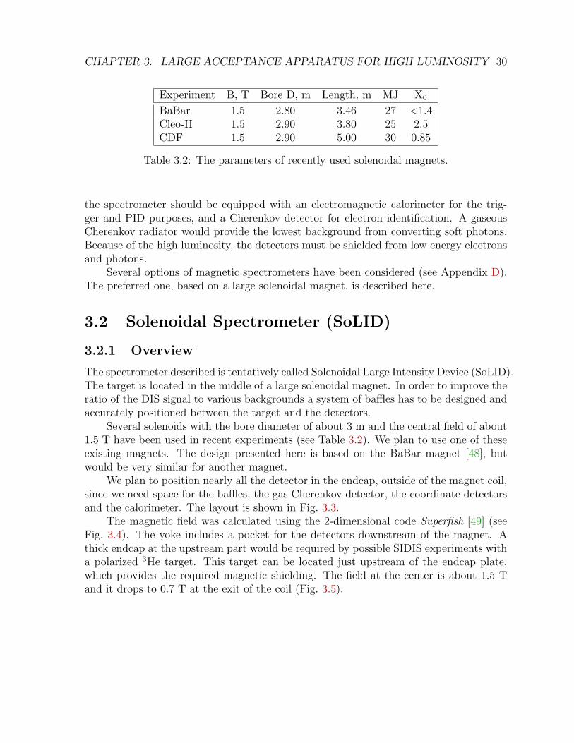
Table 3.2: The parameters of recently used solenoidal magnets.
the spectrometer should be equipped with an electromagnetic calorimeter for the trig-ger and PID purposes, and a Cherenkov detector for electron identification. A gaseousCherenkov radiator would provide the lowest background from converting soft photons.Because of the high luminosity, the detectors must be shielded from low energy electronsand photons.
Several options of magnetic spectrometers have been considered (see Appendix D).The preferred one, based on a large solenoidal magnet, is described here.
3.2 Solenoidal Spectrometer (SoLID)
3.2.1 Overview
The spectrometer described is tentatively called Solenoidal Large Intensity Device (SoLID).The target is located in the middle of a large solenoidal magnet. In order to improve theratio of the DIS signal to various backgrounds a system of baffles has to be designed andaccurately positioned between the target and the detectors.
Several solenoids with the bore diameter of about 3 m and the central field of about1.5 T have been used in recent experiments (see Table 3.2). We plan to use one of theseexisting magnets. The design presented here is based on the BaBar magnet [48], butwould be very similar for another magnet.
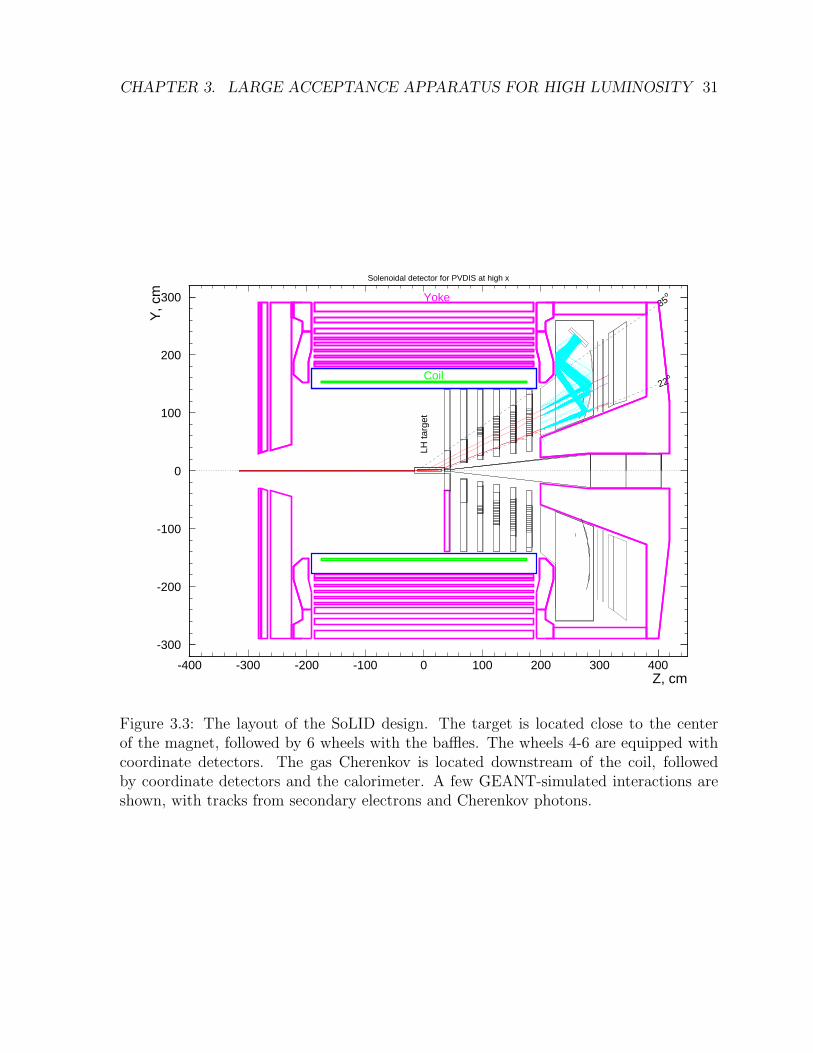
We plan to position nearly all the detector in the endcap, outside of the magnet coil,since we need space for the baffles, the gas Cherenkov detector, the coordinate detectorsand the calorimeter. The layout is shown in Fig. 3.3.
The magnetic field was calculated using the 2-dimensional code Superfish [49] (seeFig. 3.4). The yoke includes a pocket for the detectors downstream of the magnet. Athick endcap at the upstream part would be required by possible SIDIS experiments witha polarized 3He target. This target can be located just upstream of the endcap plate,which provides the required magnetic shielding. The field at the center is about 1.5 Tand it drops to 0.7 T at the exit of the coil (Fig. 3.5).
CHAPTER 3. LARGE ACCEPTANCE APPARATUS FOR HIGH LUMINOSITY 31
Solenoidal detector for PVDIS at high x
-300
-200
-100
0
100
200
300
-400 -300 -200 -100 0 100 200 300 400Z, cm
Y, c
m
LH ta
rget
Coil
Yoke
22o
35o
Figure 3.3: The layout of the SoLID design. The target is located close to the centerof the magnet, followed by 6 wheels with the baffles. The wheels 4-6 are equipped withcoordinate detectors. The gas Cherenkov is located downstream of the coil, followedby coordinate detectors and the calorimeter. A few GEANT-simulated interactions areshown, with tracks from secondary electrons and Cherenkov photons.

CHAPTER 3. LARGE ACCEPTANCE APPARATUS FOR HIGH LUMINOSITY 32
BaBar Magnet for PVDIS & transversity, attempts to compensate the axial force
C:\my_poisson\BABAR_TRANSV_3_4.AM 10−28−2008 1:55:44
0
50
100
150
200
250
300
350
400
450
500
0
50
100
150
200
250
300
350
400
450
500
300 400 500 600 700 800 900 1000
Figure 3.4: The Superfish [49] calculation of the magnetic field in the BaBar solenoidwith a custom yoke. The barrel part of the yoke is identical to the BaBar yoke, therest is optimized for both PVDIS and SIDIS type of experiments. The latter needs asmall magnetic field in the target area, upstream of the frontal endcap. In spite of theasymmetric yoke the residual axial force on the coil is small and within the tolerance.
00.20.40.60.8
11.21.41.61.8
-200 0 200Z, cm
B, T BZ at X=Y=0
BT for θ=30o
Figure 3.5: The magnetic field along the Z-axis (see also Fig. 3.4), and the field perpen-dicular to a particle trajectory at θ = 30.
CHAPTER 3. LARGE ACCEPTANCE APPARATUS FOR HIGH LUMINOSITY 33
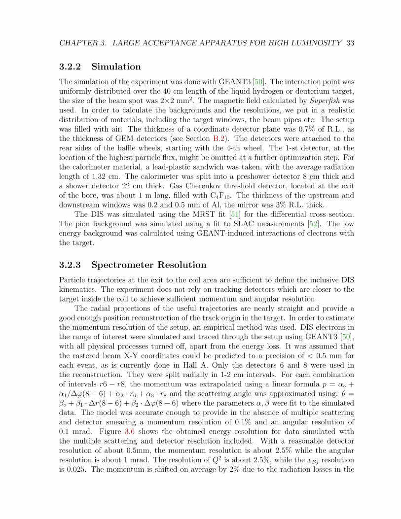
3.2.2 Simulation
The simulation of the experiment was done with GEANT3 [50]. The interaction point wasuniformly distributed over the 40 cm length of the liquid hydrogen or deuterium target,the size of the beam spot was 2×2 mm2. The magnetic field calculated by Superfish wasused. In order to calculate the backgrounds and the resolutions, we put in a realisticdistribution of materials, including the target windows, the beam pipes etc. The setupwas filled with air. The thickness of a coordinate detector plane was 0.7% of R.L., asthe thickness of GEM detectors (see Section B.2). The detectors were attached to therear sides of the baffle wheels, starting with the 4-th wheel. The 1-st detector, at thelocation of the highest particle flux, might be omitted at a further optimization step. Forthe calorimeter material, a lead-plastic sandwich was taken, with the average radiationlength of 1.32 cm. The calorimeter was split into a preshower detector 8 cm thick anda shower detector 22 cm thick. Gas Cherenkov threshold detector, located at the exitof the bore, was about 1 m long, filled with C4F10. The thickness of the upstream anddownstream windows was 0.2 and 0.5 mm of Al, the mirror was 3% R.L. thick.
The DIS was simulated using the MRST fit [51] for the differential cross section.The pion background was simulated using a fit to SLAC measurements [52]. The lowenergy background was calculated using GEANT-induced interactions of electrons withthe target.
3.2.3 Spectrometer Resolution
Particle trajectories at the exit to the coil area are sufficient to define the inclusive DISkinematics. The experiment does not rely on tracking detectors which are closer to thetarget inside the coil to achieve sufficient momentum and angular resolution.
The radial projections of the useful trajectories are nearly straight and provide agood enough position reconstruction of the track origin in the target. In order to estimatethe momentum resolution of the setup, an empirical method was used. DIS electrons inthe range of interest were simulated and traced through the setup using GEANT3 [50],with all physical processes turned off, apart from the energy loss. It was assumed thatthe rastered beam X-Y coordinates could be predicted to a precision of < 0.5 mm foreach event, as is currently done in Hall A. Only the detectors 6 and 8 were used inthe reconstruction. They were split radially in 1-2 cm intervals. For each combinationof intervals r6 − r8, the momentum was extrapolated using a linear formula p = α +α1/∆ϕ(8 − 6) + α2 · r6 + α3 · r8 and the scattering angle was approximated using: θ =β + β1 ·∆r(8− 6) + β2 ·∆ϕ(8− 6) where the parameters α, β were fit to the simulateddata. The model was accurate enough to provide in the absence of multiple scatteringand detector smearing a momentum resolution of 0.1% and an angular resolution of0.1 mrad. Figure 3.6 shows the obtained energy resolution for data simulated withthe multiple scattering and detector resolution included. With a reasonable detectorresolution of about 0.5mm, the momentum resolution is about 2.5% while the angularresolution is about 1 mrad. The resolution of Q2 is about 2.5%, while the xBj resolutionis 0.025. The momentum is shifted on average by 2% due to the radiation losses in the
CHAPTER 3. LARGE ACCEPTANCE APPARATUS FOR HIGH LUMINOSITY 34
0
0.01
0.02
0.03
0.04
0.05
0.06
0.07
25 30 350
0.025
0.05
0.075
0.1
0.125
0.15
0.175
0.2
0.225
x 10-2
25 30 35
0
0.01
0.02
0.03
0.04
0.05
0.06
0.07
25 30 350
0.01
0.02
0.03
0.04
0.05
0.06
0.07
0.08
25 30 35
Figure 3.6: The spectrometer resolutions (RMS) in momentum p and the scattering angleθ, as well as the derived DIS variables Q2 and xBj. The resolutions are calculated for 4different position resolutions of the detectors.
material. The ϕ resolution is about 3 mrad.
3.2.4 Baffles
The solenoidal field shields the detectors from charged particles with p < 0.3 GeV.However, a high rate of photons coming from the target, as well as a high flux of low mo-mentum pions p > 0.3 GeV, would limit the operations of the spectrometer discussed. Arelatively narrow momentum spectrum of the particles of interest allows us to implementa system of baffles which would filter out both strongly bending low momentum parti-cles and straight photons. Several disk-shaped absorbers can be inserted downstreamof the target. These disks should have sets of relatively narrow slits, which form chan-nels, shaped in order to let the useful particles produced in a certain azimuthal range∆ϕ to pass through. The goal is to provide an overall acceptance of 30-50% of the fullazimuthal coverage of 2π, for the scattered electrons in the selected range. One shouldtry to maximize the value of ∆ϕ in order to simplify the geometry and reduce the effects

CHAPTER 3. LARGE ACCEPTANCE APPARATUS FOR HIGH LUMINOSITY 35
of slit scattering.In the reference frame used the axis Z pointed along the beam. The solenoid mag-
netic field turned electrons toward larger values of the azimuthal angle ϕ. After severaliterations an approximate ϕ range was defined, as ∆ϕ(θ) = 5+4 · (θ−22)/(35−22).In total, 6 absorber disks (or wheels) were considered, located at the following Z-positions(in cm): 30. 60. 90. 120. 150. 180.
Each disk contains 30 curved slits. The slits’ shape was optimized in two stepsin a semi-automatic procedure. First, the GEANT-simulated tracks in the kinematicregion of interest, in a defined ϕ range, were used to maximize the acceptance to thesetracks. A small line-of-sight aperture to the target remained, allowing direct photon fluxdownstream of the 6th baffle. The slits were adjusted to block these photons completely,with miminal cost to the useful acceptance. The baffles geometry is shown in Fig. 3.7.For the full GEANT simulation the baffles were assumed to be made of lead 9 cm thick(20 R.L.). The slits were cut just perpendicular to the surface of the disk.
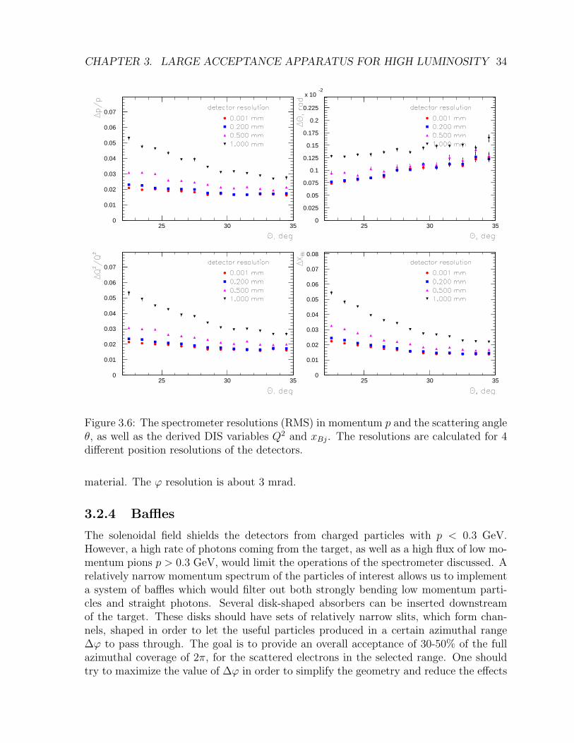
Below 1.5 GeV, the baffles eliminate the electrons and reduce the pions by a factorof 20-30 (see Fig. 3.8).
Figure 3.7: The optimized geometry of the baffles.
CHAPTER 3. LARGE ACCEPTANCE APPARATUS FOR HIGH LUMINOSITY 36
Figure 3.8: The acceptance dependence on the particle momentum for electrons andpions. The baffles reject electrons with p < 1.5 GeV, while pions below 1.5 GeV arereduced by a factor of 20-50.
CHAPTER 3. LARGE ACCEPTANCE APPARATUS FOR HIGH LUMINOSITY 37
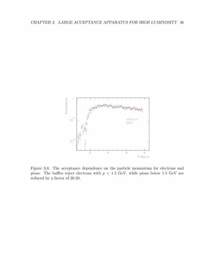
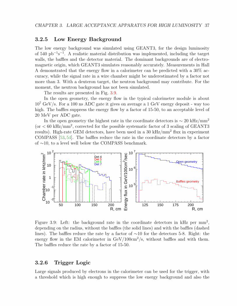
3.2.5 Low Energy Background
The low energy background was simulated using GEANT3, for the design luminosityof 540 pb−1s−1. A realistic material distribution was implemented, including the targetwalls, the baffles and the detector material. The dominant backgrounds are of electro-magnetic origin, which GEANT3 simulates reasonably accurately. Measurements in HallA demonstrated that the energy flow in a calorimeter can be predicted with a 30% ac-curacy, while the signal rate in a wire chamber might be underestimated by a factor notmore than 3. With a deuteron target, the neutron background may contribute. For themoment, the neutron background has not been simulated.
The results are presented in Fig. 3.9.In the open geometry, the energy flow in the typical calorimeter module is about
107 GeV/s. For a 100 ns ADC gate it gives on average a 1 GeV energy deposit - way toohigh. The baffles suppress the energy flow by a factor of 15-50, to an acceptable level of20 MeV per ADC gate.
In the open geometry the highest rate in the coordinate detectors is ∼ 20 kHz/mm2
(or < 60 kHz/mm2, corrected for the possible systematic factor of 3 scaling of GEANT3results). High-rate GEM detectors, have been used in a 30 kHz/mm2 flux in experimentCOMPASS [53, 54]. The baffles reduce the rate in the coordinate detectors by a factorof ∼10, to a level well below the COMPASS benchmark.
10-2
10-1
1
10
10 2
50 100 150 200R, cm
Cha
mbe
r ra
te in
kH
z/m
m2
Det 4Det 5Det 6Det 7
10 5
10 6
10 7
125 150 175 200R, cmE
nerg
y flu
x in
GeV
/100
cm2 /s
ec
Open geometry
Baffles geometry
Figure 3.9: Left: the background rate in the coordinate detectors in kHz per mm2,depending on the radius, without the baffles (the solid lines) and with the baffles (dashedlines). The baffles reduce the rate by a factor of ∼10 for the detectors 5-8. Right: theenergy flow in the EM calorimeter in GeV/100cm2/s, without baffles and with them.The baffles reduce the rate by a factor of 15-50.
3.2.6 Trigger Logic
Large signals produced by electrons in the calorimeter can be used for the trigger, witha threshold which is high enough to suppress the low energy background and also the
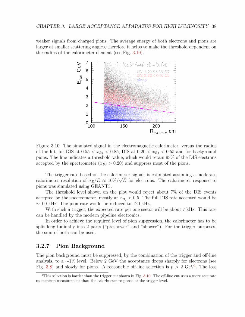
CHAPTER 3. LARGE ACCEPTANCE APPARATUS FOR HIGH LUMINOSITY 38
weaker signals from charged pions. The average energy of both electrons and pions arelarger at smaller scattering angles, therefore it helps to make the threshold dependent onthe radius of the calorimeter element (see Fig. 3.10).
0
1
2
3
4
5
6
7
100 150 200RCALOR, cm
EC
AL
GeV
Figure 3.10: The simulated signal in the electromagnetic calorimeter, versus the radiusof the hit, for DIS at 0.55 < xBj < 0.85, DIS at 0.20 < xBj < 0.55 and for backgroundpions. The line indicates a threshold value, which would retain 93% of the DIS electronsaccepted by the spectrometer (xBj > 0.20) and suppress most of the pions.
The trigger rate based on the calorimeter signals is estimated assuming a moderatecalorimeter resolution of σE/E ≈ 10%/
√E for electrons. The calorimeter response to
pions was simulated using GEANT3.The threshold level shown on the plot would reject about 7% of the DIS events
accepted by the spectrometer, mostly at xBj < 0.5. The full DIS rate accepted would be∼100 kHz. The pion rate would be reduced to 120 kHz.
With such a trigger, the expected rate per one sector will be about 7 kHz. This ratecan be handled by the modern pipeline electronics.
In order to achieve the required level of pion suppression, the calorimeter has to besplit longitudinally into 2 parts (“preshower” and “shower”). For the trigger purposes,the sum of both can be used.
3.2.7 Pion Background
The pion background must be suppressed, by the combination of the trigger and off-lineanalysis, to a ∼1% level. Below 2 GeV the acceptance drops sharply for electrons (seeFig. 3.8) and slowly for pions. A reasonable off-line selection is p > 2 GeV1. The loss
1This selection is harder than the trigger cut shown in Fig. 3.10. The off-line cut uses a more accuratemomentum measurement than the calorimeter response at the trigger level.

CHAPTER 3. LARGE ACCEPTANCE APPARATUS FOR HIGH LUMINOSITY 39
is about 4% of all DIS events, mostly in a range 0.3 < xBj < 0.5. The pion to electronratio within the acceptance (Fig. 3.11) is about 102 at 2 GeV.
10
10 2
10 3
1 2 3 4P, GeV/c
π/e
ratio
with
in a
ccep
tanc
e
Figure 3.11: Pion to electron ratio, as a function of particle momentum for the particleswithin the geometric acceptance.
One can obtain a suppression factor of ∼ 2 · 105 [55] for pions, using an electro-magnetic calorimeter and a gas Cherenkov threshold detector. The calorimeter has tobe segmented longitudinally into a “preshower” and “shower” parts. With such a sup-pression factor the pion background would be ∼0.1% at 2 GeV and would drop at largermomenta. At p > 3 GeV the π/e ratio is < 10. This can be reduced to 1% with the helpof the calorimeter only.
Due to low energy backgrounds, the proposed experiment will require detectors withat least the same performance, and perhaps with better timing, than the lead-glasscalorimeter and the CO2-filled, 130 cm long gas Cherenkov detector used in [55].
3.2.8 Acceptance and Rates
The xBj−Q2 plot of the DIS events accepted is shown in Fig. 3.12 (left), for 11 GeV beam.The acceptance is nearly flat at xBj > 0.5 and drops from 37% to 25% at xBj = 0.4, asshown in Fig. 3.12, right. The rates calculated (see also Section 3.2.6) for hydrogen withL ∼ 540 pb−1s−1, under various conditions, are presented in Table 3.3. The total triggerrate is estimated to be below 220 kHz. The DIS rate in the region xBj > 0.65 is about3 kHz.
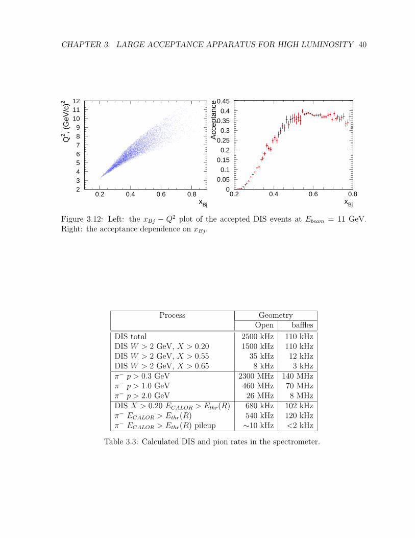
CHAPTER 3. LARGE ACCEPTANCE APPARATUS FOR HIGH LUMINOSITY 40
23456789
101112
0.2 0.4 0.6 0.8xBj
Q2 , (
GeV
/c)2
0
0.05
0.1
0.15
0.2
0.25
0.3
0.35
0.4
0.45
0.2 0.4 0.6 0.8xBj
Acc
epta
nce
Figure 3.12: Left: the xBj − Q2 plot of the accepted DIS events at Ebeam = 11 GeV.Right: the acceptance dependence on xBj.
Process GeometryOpen baffles
DIS total 2500 kHz 110 kHzDIS W > 2 GeV, X > 0.20 1500 kHz 110 kHzDIS W > 2 GeV, X > 0.55 35 kHz 12 kHzDIS W > 2 GeV, X > 0.65 8 kHz 3 kHzπ− p > 0.3 GeV 2300 MHz 140 MHzπ− p > 1.0 GeV 460 MHz 70 MHzπ− p > 2.0 GeV 26 MHz 8 MHzDIS X > 0.20 ECALOR > Ethr(R) 680 kHz 102 kHzπ− ECALOR > Ethr(R) 540 kHz 120 kHzπ− ECALOR > Ethr(R) pileup ∼10 kHz <2 kHz
Table 3.3: Calculated DIS and pion rates in the spectrometer.
CHAPTER 3. LARGE ACCEPTANCE APPARATUS FOR HIGH LUMINOSITY 41
3.2.9 Implementation
Possible technical solutions for the Solenoidal Large Intensity Device (SoLID) are dis-cussed in details in Section B. For some systems robust solutions already exist. Otherswill require R&D, on implementing existing technologies to the particular case.
Chapter 4
Beam and Target
4.1 Beam
In this section we describe the preparation of the beam, the control of beam-related sys-tematic errors and beam-related noise. The excellent quality of the beam at Jefferson Labhas made feasible parity experiments with much smaller asymmetries than this proposal.The random fluctuations in beam parameters are small enough to not add significantnoise to the measurements. For the polarized source we have a well-developed modelfor controlling the laser systematics, which allows us to minimize helicity correlationsin the laser beam used to produce polarized electrons. For the accelerator, we have awell-developed procedure for betatron matching that achieves maximum dampening ofposition differences. For the 11 GeV running we will require the upgrade of the ARCenergy measurement apparatus, which is already planned.
For parity experiments, the physical properties of the beam need to be identicalfor the left- and right-handed beams to a very high degree so as to minimize spuriousasymmetries. The helicity-correlated intensity asymmetry will be maintained to be lessthan 1 ppm by an active feedback loop. The physical properties of the electron beam willbe monitored with high precision by beam monitors, both stripline and cavity monitors.A luminosity monitor downstream of the target will monitor target density fluctuations,which are not expected to be a problem for this proposal. Although the main DAQ forthis experiment is a counting-mode DAQ, for the purposes of studying helicity-correlatedbeam properties, the beam monitors and possibly other detectors could be simultaneou-osly read out by the existing HAPPEX DAQ which integrates over the helicity period.
At the polarized source, a GaAs photocathode is optically pumped by circularly po-larized laser light to produce polarized electrons, with the ability to rapidly and randomlyflip the sign of the electron beam polarization. The asymmetry is extracted by generatingthe incident electron beam as a pseudorandom time sequence of helicity “windows” at30 Hz and then measuring the fractional difference in the integrated scattered flux overwindow pairs of opposite helicity.
The electron beam polarization will be measured by Møller scattering and Comptonscattering (section 5.3).
42
CHAPTER 4. BEAM AND TARGET 43
To measure the sensitivity of the scattered flux to beam parameters we may combineour counting-mode DAQ for the detectors with the integrating-mode DAQ for beamlineelements, and we may spend a fraction of our beam time (∼ 2%) making modulations ofbeam parameters by modulating corrector coils in the beam line leading to the target,as well as a klystron which modulates energy.
To measure the beam intensity, microwave cavity BCMs have been developed atJefferson Lab. The precision that has been achieved for a 30 ms beam window at 100µA is 4 × 10⁻⁵. This superior resolution is a result of the high quality of the JLabbeam, the good radiofrequency (rf) instrumentation, as well as a custom high resolutionADCs. During the 2005 HAPPEX run we achieved helicity correlated position differencesaveraged over 1-month at the ∼1 nanometer level. These performances are more thanadequate for this proposal.
4.2 Target
For this proposal we plan to build 40-cm long cyrogenic liquid hydrogen and deuteriumtargets. Jefferson Lab has extensive experience with cyrogenic targets, although they arenormally 20 to 25 cm long. The two available designs of the cryotarget cell which canfulfill our requirements are a racetrack-shaped (as used in HAPPEX-II) and cylindrical a(“cigar-tube”) cells. Racetrack cells have much better cooling flow and thus have provedto be more suitable to avoid boiling effects. However, due to our low rates the boilingeffects are not expected to be a problem, as explained further below.
For the 6 GeV PVDIS experiment, expected to run in the Fall of 2009, will use a25-cm LD2 target with 100 µA. The main change for this proposal is a longer cell, 40-cm,which at 50 µA beam current would require 25% more cooling capacity. An increase incooling capacity is already foreseen for the lab. For example, the Qweak experiment willrun with 180µA on a 35-cm LH2 target.
The endcaps of a typical target cell at JLab are made of 10 mil aluminum (AL 7075-T6). For the G0 experiment, a special cell was made with Al endcaps 5 mils thick. Thiswill be sufficient for this experiment to maintain an acceptable level of background. Thebackground ratio from endcaps will be measured in the standard way using an emptytarget with the same endcaps as the target cells, a “dummy” cell. The radiation lengthof the thick dummy cell will be made the same as the cryogenic cells so that radiativelosses are similar. The asymmetry of ~e−Al DIS could be somewhat different from Ad orAh. We plan to measure the ~e−Al DIS asymmetry during the approved 6 GeV PVDISexperiment. If necessary this asymmetry could also be measured during this experimentusing an empty target with thick Al endcaps,
Target boiling effects are not expected to be a problem for this experiment becausethe statistical accuracy in a given helicity period is much larger than the expected noisefrom boiling. There are two effects commonly termed “target boiling”. One is due toa phase change in the liquid which reduces the rate; this should be less than 5% forthis experiment. The second meaning of “target boiling” which is more relevant forparity-violation, is pulse-to-pulse density fluctuations induced by beam parameters such

CHAPTER 4. BEAM AND TARGET 44
as spot size. This causes noise in the measured asymmetry. Based on the experiencewith cryogenic targets at JLab we don’t expect the noise to be significant comparedto counting statistics. A luminosity monitor placed downstream is commonly used tomonitor the density fluctuation noise.
The hydrogen target may become polarized in the magnetic field of the solenoid. Thiswould cause an asymmetry unrelated to the weak interaction physics of the experiment.The strategy for depolarizing the targets may be different for the two targets becauseof their different spin relaxation timescales. For the deuterium target we may use anRF depolarizer, while for the hydrogen the plan would be to start with relatively purepara-hydrogen. Catalysis by interaction with surface materials in the target loop mightalso help depolarize the hydrogen target. Small residual polarizations that may remaincan be cancelled by flipping the polarity of the field in some running periods.
Chapter 5
Systematic Corrections
5.1 Kinematic Reconstruction
In order to reconstruct the kinematic quantities of interest, i.e. Q2, xBj, etc, we will needprecise measurements of the beam energy Eb, the scattering angle θ and the final-stateenergy E ′ as well as having good PID for the scattered particle. The PID is provided bythe electromagnetic calorimeter (ECAL) shower and preshower data combined with theCherenkov detector data.
The general strategy is to rely on the excellent knowledge of Eb and to calibratethe apparatus with elastic scattering. The scattering angle may be reconstructed with∼ 0.5 mrad accuracy using the high-resolution GEM tracking information and precisemeasurements of the detector positions. We plan to map out the magnetic field in thetracking area, for the momentum reconstruction. Additionally, we plan to use the elasticscattering off hydrogen at beam energies of 4.4 and 6.6 GeV to calibrate the measurementsof the momentum and Q2. With the expected spectrometer resolution, at 4.4 GeV theelastic peak will be separated from the inelastic background, with a contamination fromthe latter of about 5%. At 6.6 GeV the contamination will be about 25%. Since theexpected rate at the full luminosity will be high (50 kHz at 4.4 GeV and 4 kHz at 6.6GeV) further optimization of the calibration conditions are possible, for example usingthinner targets or running at a low current. Comparing the elastic peaks at two beamenergies will allow to cross-check both the momentum and the angle scales, and calibratethe Q2 measurement to a 0.2% accuracy.
Several options exist to increase the accuracy further. They will be consideredat the next stage of development. For a better selection of the elastic events one candetect the recoil proton, which, for the given electron kinematics, mostly stays withinthe acceptance of the spectrometer. For this, we will need to be able to rotate the bafflewheels in order to allow positively charged particles to come through. Another possibilityis to make calibration runs without the baffles, and at much lower luminosity. Note thatthe beam position and current monitors are already being upgraded to achieve goodaccuracy (better than 0.1 mm in position) at very low currents (down to 0.1 nA).
Measurements of beam energy Eb to better than 10−3 accuracy are routine at JLab,
45
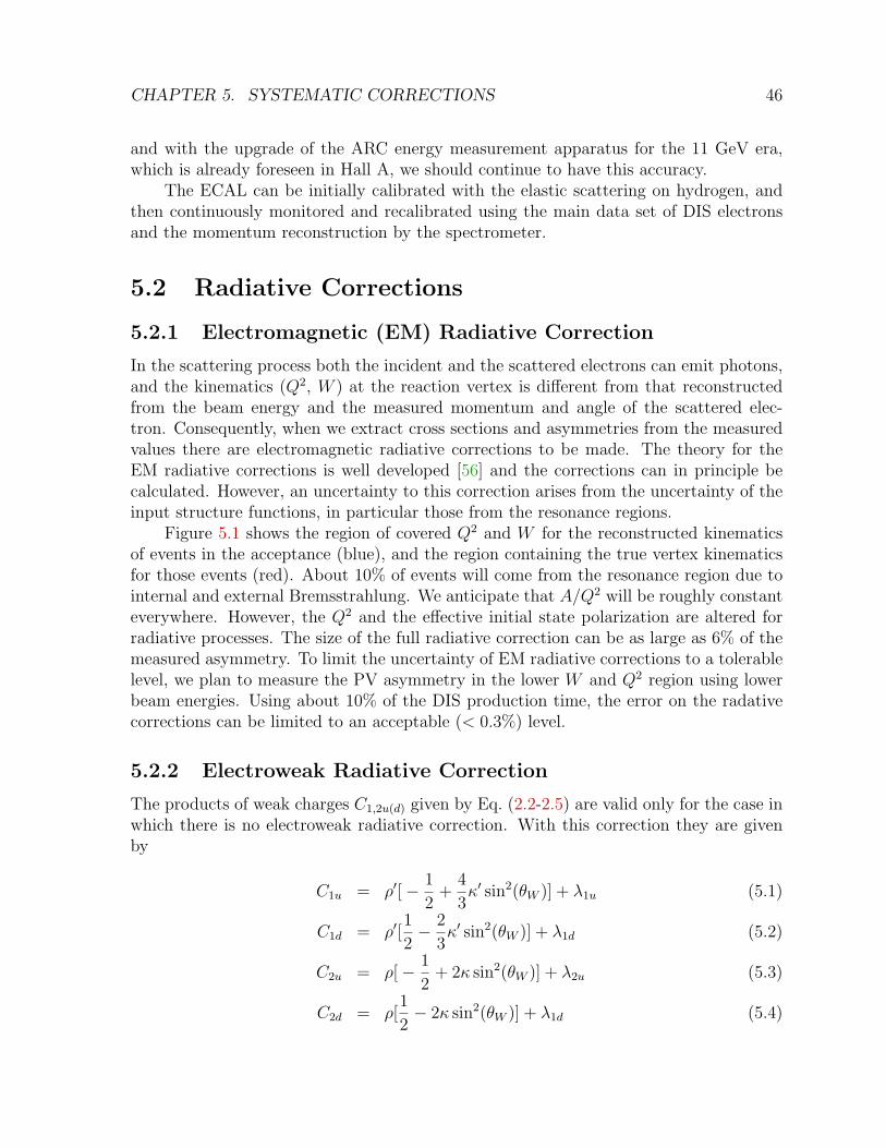
CHAPTER 5. SYSTEMATIC CORRECTIONS 46
and with the upgrade of the ARC energy measurement apparatus for the 11 GeV era,which is already foreseen in Hall A, we should continue to have this accuracy.
The ECAL can be initially calibrated with the elastic scattering on hydrogen, andthen continuously monitored and recalibrated using the main data set of DIS electronsand the momentum reconstruction by the spectrometer.
5.2 Radiative Corrections
5.2.1 Electromagnetic (EM) Radiative Correction
In the scattering process both the incident and the scattered electrons can emit photons,and the kinematics (Q2, W ) at the reaction vertex is different from that reconstructedfrom the beam energy and the measured momentum and angle of the scattered elec-tron. Consequently, when we extract cross sections and asymmetries from the measuredvalues there are electromagnetic radiative corrections to be made. The theory for theEM radiative corrections is well developed [56] and the corrections can in principle becalculated. However, an uncertainty to this correction arises from the uncertainty of theinput structure functions, in particular those from the resonance regions.
Figure 5.1 shows the region of covered Q2 and W for the reconstructed kinematicsof events in the acceptance (blue), and the region containing the true vertex kinematicsfor those events (red). About 10% of events will come from the resonance region due tointernal and external Bremsstrahlung. We anticipate that A/Q2 will be roughly constanteverywhere. However, the Q2 and the effective initial state polarization are altered forradiative processes. The size of the full radiative correction can be as large as 6% of themeasured asymmetry. To limit the uncertainty of EM radiative corrections to a tolerablelevel, we plan to measure the PV asymmetry in the lower W and Q2 region using lowerbeam energies. Using about 10% of the DIS production time, the error on the radativecorrections can be limited to an acceptable (< 0.3%) level.
5.2.2 Electroweak Radiative Correction
The products of weak charges C1,2u(d) given by Eq. (2.2-2.5) are valid only for the case inwhich there is no electroweak radiative correction. With this correction they are givenby
C1u = ρ′[− 1
2+
4
3κ′ sin2(θW )] + λ1u (5.1)
C1d = ρ′[1
2− 2
3κ′ sin2(θW )] + λ1d (5.2)
C2u = ρ[− 1
2+ 2κ sin2(θW )] + λ2u (5.3)
C2d = ρ[1
2− 2κ sin2(θW )] + λ1d (5.4)
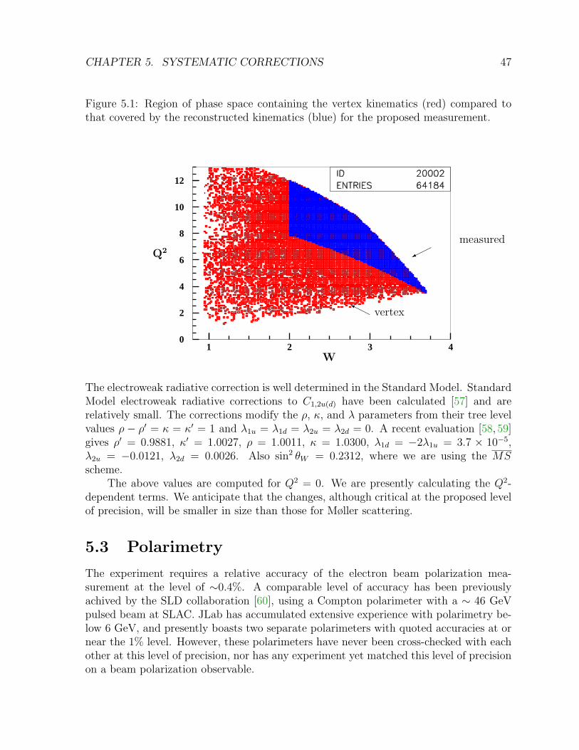
CHAPTER 5. SYSTEMATIC CORRECTIONS 47
Figure 5.1: Region of phase space containing the vertex kinematics (red) compared tothat covered by the reconstructed kinematics (blue) for the proposed measurement.
0
2
4
6
8
10
12
1 2 3 4
vertex Q2 vs W with cut Wrecon2
measured
HHY vertex
W
Q2
The electroweak radiative correction is well determined in the Standard Model. StandardModel electroweak radiative corrections to C1,2u(d) have been calculated [57] and arerelatively small. The corrections modify the ρ, κ, and λ parameters from their tree levelvalues ρ − ρ′ = κ = κ′ = 1 and λ1u = λ1d = λ2u = λ2d = 0. A recent evaluation [58, 59]gives ρ′ = 0.9881, κ′ = 1.0027, ρ = 1.0011, κ = 1.0300, λ1d = −2λ1u = 3.7 × 10⁻⁵,λ2u = −0.0121, λ2d = 0.0026. Also sin2 θW = 0.2312, where we are using the MSscheme.
The above values are computed for Q2 = 0. We are presently calculating the Q2-dependent terms. We anticipate that the changes, although critical at the proposed levelof precision, will be smaller in size than those for Møller scattering.
5.3 Polarimetry
The experiment requires a relative accuracy of the electron beam polarization mea-surement at the level of ∼0.4%. A comparable level of accuracy has been previouslyachived by the SLD collaboration [60], using a Compton polarimeter with a ∼ 46 GeVpulsed beam at SLAC. JLab has accumulated extensive experience with polarimetry be-low 6 GeV, and presently boasts two separate polarimeters with quoted accuracies at ornear the 1% level. However, these polarimeters have never been cross-checked with eachother at this level of precision, nor has any experiment yet matched this level of precisionon a beam polarization observable.

CHAPTER 5. SYSTEMATIC CORRECTIONS 48
The prospects for improving polarimetery at JLab to the necessary level are good.Upcoming experiments in the JLab “6 GeV” program, in both Halls A and C, require1% polarimetry [61,62,14,63]. These requirements will lead to the upgrade of the Hall ACompton polarimeter, the development of a Hall C Compton polarimeter and improve-ments to existing Moller polarimeters which use ferromagnetic foil targets. These 6 GeVexperiments will be an excellent introductory challenge to very high-accuracy polarime-try at JLab, and should sharpen techniques both in controlling systematic uncertaintiesand in cross-comparing high-precision polarimeters.
In order to reach a robust 0.4% accuracy, we propose to develop two separate, con-tinuous polarimeters for the current proposal, each independently normalized to thatlevel of accuracy. Each polarimeter should provide a 0.4% statistical precision in compa-rable time periods of not more than several hours, in order to facilitate cross-checks andsystematic studies. This redundancy, both in the measurement and monitoring of thebeam polarization, will provide a new benchmark in precision electron beam polarimetry.We discuss both polarimeters in extensive detail in Sec. C.2 and Sec. C.1.
Chapter 6
Concluding Remarks
6.1 Collaboration
The collaboration is quite diverse, including experts of precise parity experiments such asQweak, G0, HAPPEX, SLAC E158. We also have groups with the experience to developand build the necessary hardware. Theoretical support for PVDIS is being provided bycollaborators J. Erler and M. Ramsey-Musolf.
6.2 Synergy with Other Proposals
There is significant overlap between the PVDIS and Moller experimental collaborations.This ensures ample expertise in the special issues related to parity experiments. Thepolarimeters will be shared by both experiments. Since the total fractional error forPVDIS is 0.6%, the demands on polarimetry are more severe. However, since the Møllerexperiment needs to be strictly statistics limited, our specified precision of 0.4% is veryuseful for them.
The SIDIS collaboration is also submitting a proposal using the solenoid to makecoincidence measurements with a polarized 3He target. While there are significant dif-ferences in the configurations for PVDIS and SIDIS, much of the hardware is shared. Ifboth proposals are approved, we plan to work closely together on both experiments.
6.3 Beam Request
For the deuterium data, we have based our sensitivity on 180 days of production runningat 50 µA, with 1/3 of the data at 6.6 GeV and the rest at 11 GeV. Approximately 27additional days, run at various currents, will be required for checkout and calibrations.An additional 18 days will be required at 4.4 GeV and 50 µA for radiative correctionmeasurements. The total beam request at all energies for the deuterium measurement is225 days, with about 25 of those days run mostly at reduced beam currents.
49

CHAPTER 6. CONCLUSION 50
For the hydrogen meausrement, 90 days are needed for production data at 11 GeV,about 9 days are required at 4.4 GeV to control radiative corrections and another 14days will be required for calibration. The running time requested for hydrogen totals to113 days.
In the future, we would also anticipate requesting an additional comparable run fora heavy nucleus such as Pb.
6.4 Cost and Schedule
We are preparing a preliminary cost estimate for the project. However, it is already clearthat significant funds will be required from several agencies. We plan to seek fundingfrom the US DOE, NSF, and international sources. As emphasized earlier, this projecthas been listed in the Fundamental Symmetries initiative in the NSAC Long Range Plan,and has been included in the Plan’s 10 year funding profile.
Assuming that we receive the endorsement of the JLab PAC, we will request atechnical review by the end of 2009 so that we can start seeking funding from the agenciesearly in 2010. The goal is to start construction by 2012 and schedule installation for 2015.
6.5 Assignment of Tasks
We list below key subsystems and institutions who are interested in design, constructionand implementation of them. Note that these are not firm or binding responsibilities, butsimply the current thinking of the collaboration given each institution’s current interestsand past experience. As emphasized earlier, we expect the collaboration to expand shouldwe receive PAC approval.
• Polarized source: UVa, JLab
• Cryo Target: JLab, MissSt
• Magnet: UMass, JLab, MIT, ANL
• Baffles: Longwood
• Tracking Detectors: UVa, Seoul Nat’l, Kentucky, William and Mary, MissSt,China Collaboration (USTC, Beijing, China IAE, Lanzhou, Tsinghua, Huangshan)
• Gas Cerenkov: Temple, ANL, Ohio
• Shower: William and Mary, Syracuse, UMass, Rutgers, VaTech
• Electronics: JLab
• Polarimetry: UVa, Syracuse, JLab, CMU, ANL, MissSt
• Data Acquisition: UVa, JLab, LANL, Ohio, LaTech
• Simulations: Longwood, JLab, UVa, LaTech

Appendix A
Physics
A.1 DIS Phenomenology
In order to make a precise comparison of the data with theory, a more careful treatmentof the asymmetry must be used [1]. The cross section can be written formally in termsof products of hadronic and leptonic tensors.
d2σ
dΩde′=α2
Q4
E ′
E
(Lγ
µνWµνγ +
GF
4√
2παLγZ
µνWµνγZ
)
The lepton tensor for the interference term is related to the electromagnetic lepton tensor
Lγµν = 2(lµl
′ν + l′µlν − l · l′gµν + iλεµναβl
αl′β)
byLγZ
µν = (geV + λge
A)Lγµν
where λ is 1 (-1) for positive (negative) helicity of the initial lepton beam.For the hadronic tensors, we can write
W γ(γZ)µν =
1
2M
∑X
〈X|Jγ(Z)µ |N〉∗〈X|Jγ
µ |N〉
+ 〈X|Jγµ |N〉∗〈X|Jγ(Z)
µ |N〉(2π)2δ(PX − p− q) (A.1)
where Jγ(Z)µ is the hadronic electromagnetic (weak) current and M is the nucleon mass,
and N is the target nucleus.For unpolarized targets, the hadronic current can be decomposed into three struc-
ture functions F ji where i = γ is the purely electromagnetic tensor and j = γZ is the
interference tensor:
W jµν = −gµν
MF j
1 +pµpν
Mp · qF j
2 +iεµναβp
αpβ
2Mp · qF j
3
The F ji are fucntions of x and Q2 only. They do not depend on y.
51
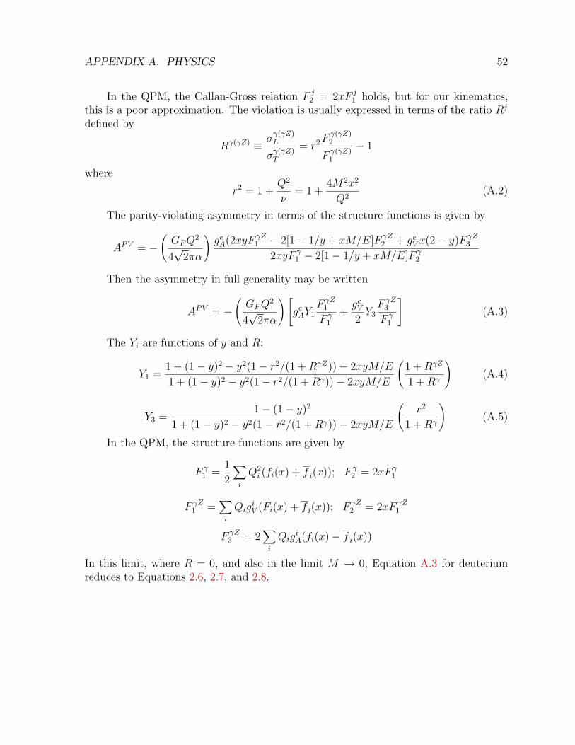
APPENDIX A. PHYSICS 52
In the QPM, the Callan-Gross relation F j2 = 2xF j
1 holds, but for our kinematics,this is a poor approximation. The violation is usually expressed in terms of the ratio Rj
defined by
Rγ(γZ) ≡ σγ(γZ)L
σγ(γZ)T
= r2Fγ(γZ)2
Fγ(γZ)1
− 1
where
r2 = 1 +Q2
ν= 1 +
4M2x2
Q2(A.2)
The parity-violating asymmetry in terms of the structure functions is given by
APV = −(GFQ
2
4√
2πα
)ge
A(2xyF γZ1 − 2[1− 1/y + xM/E]F γZ
2 + geV x(2− y)F γZ
3
2xyF γ1 − 2[1− 1/y + xM/E]F γ
2
Then the asymmetry in full generality may be written
APV = −(GFQ
2
4√
2πα
)[ge
AY1F γZ
1
F γ1
+ge
V
2Y3F γZ
3
F γ1
](A.3)
The Yi are functions of y and R:
Y1 =1 + (1− y)2 − y2(1− r2/(1 +RγZ))− 2xyM/E
1 + (1− y)2 − y2(1− r2/(1 +Rγ))− 2xyM/E
(1 +RγZ
1 +Rγ
)(A.4)
Y3 =1− (1− y)2
1 + (1− y)2 − y2(1− r2/(1 +Rγ))− 2xyM/E
(r2
1 +Rγ
)(A.5)
In the QPM, the structure functions are given by
F γ1 =
1
2
∑i
Q2i (fi(x) + f i(x)); F γ
2 = 2xF γ1
F γZ1 =
∑i
QigiV (Fi(x) + f i(x)); F γZ
2 = 2xF γZ1
F γZ3 = 2
∑i
QigiA(fi(x)− f i(x))
In this limit, where R = 0, and also in the limit M → 0, Equation A.3 for deuteriumreduces to Equations 2.6, 2.7, and 2.8.

Appendix B
Detector Implementation for SoLID
B.1 Solenoidal Magnet
We based our design on the properties of the BaBar magnet. The results can be partlyapplied to other similar magnets, as one from CLEO-II. The biggest difference is in thesizes and construction details of the yokes.
The BaBar magnet [64,65,66] (see Fig. B.1) contains an aluminium stabilized, thinsuperconducting solenoid and a return yoke, providing an axial central field of 1.5 T.
Figure B.1: BaBar magnet layout, taken from [66].
The winding is supported by an aluminium alloy outer cylinder, which provides hoopstrength to the coil. The coil has dimensions of 3 m in diameter and 3.7 m in length.
53

APPENDIX B. DETECTOR IMPLEMENTATION FOR SOLID 54
The current density is graded to meet the field uniformity requirements of 2%. The coilis indirectly cooled to 4.5 K using the liquid helium thermo-siphon technique and coolingchannels welded to the support cylinder. Automatic cooldown and cryogen supply to thecoil and its 40 K radiation shield is done by a helium liquefier/refrigerator via coaxial,return gas screened, flexible transfer lines. A hexagonal flux return, comprised of abarrel and two end doors provides the external flux path for the field. To accommodatethe muon detectors, the barrel and end caps are segmented into 20 plates of differentthickness. The gaps between the plates are about 3 cm wide.
The solenoid center is 3.500 m above the floor. In Hall A, the beam is 10 ft, or 3.048 mabove the floor. It is shown in Fig. B.1 that the distance from the center of the magnetto the bottom plate of the barrel yoke is 2.920 m. Therefore, if the four support piecesof the barrel are modified or rebuilt, one can provide a clearence of ∼12 cm between thebottom plate and the floor. The endcaps can slide transversally on their own supports.
The coil and the thermostat construction limits the integral axial force on the coilto about 35 t. The proposed design of the customized yoke, although asymmetric in Z,provides an acceptable residual force. The result from our preliminary, 2-dimensionalcalculations is about 2 t.
The optimal solution for the yoke still has to be evaluated, taking into accountthe costs for adapting various parts of the existing yoke against manufacturing newcustomized parts.
B.2 Coordinate Detectors
We number the potential locations for the coordinate detectors from 1 to 8. The first6 locations are just downstream of the 6 wheels with the baffles. The positions 7-8 aredownstream of the Cherenkov detector. As we have discussed in Section 3.2.3, 2 measuredspace points on the trajectories at the locations 6 and 8 (see Fig. 3.3) are sufficient to findthe track parameters. The calorimeter measurement of the shower centroid adds anotherpoint, with a spatial accuracy of ∼10 mm. For good pattern recognition in a high rateenvironment at least three space points with a good resolution must be measured. Nodetailed optimization of the detector arrangement has been done so far. Tentatively, weplan to install the detectors at the locations 5,6,7 and 8. In each location the space pointis measured. With not more than one point missing due to inefficiencies, and with a pointin the calorimeter, it should provide enough information for the pattern recognition, sincethe trajectories are nearly straight in this area.
The hit patterns and the detector arrangements are shown in Fig. B.2.The radial distribution of the low energy background in the system with the baffles
is nearly flat (Fig. 3.9). The rate expected from GEANT3 calculations is shown inTable B.1. The rates were increased by a factor of 3 in comparison with Fig. 3.9 in ordercompensate for possible underestimation of the low energy photons. Only micropatterndetectors such as GEM [53,54] or MICROMEGAS [67] can handle the hit densities at thelocations 5 and 6. For the locations 7-8 one may consider using straw detectors similar
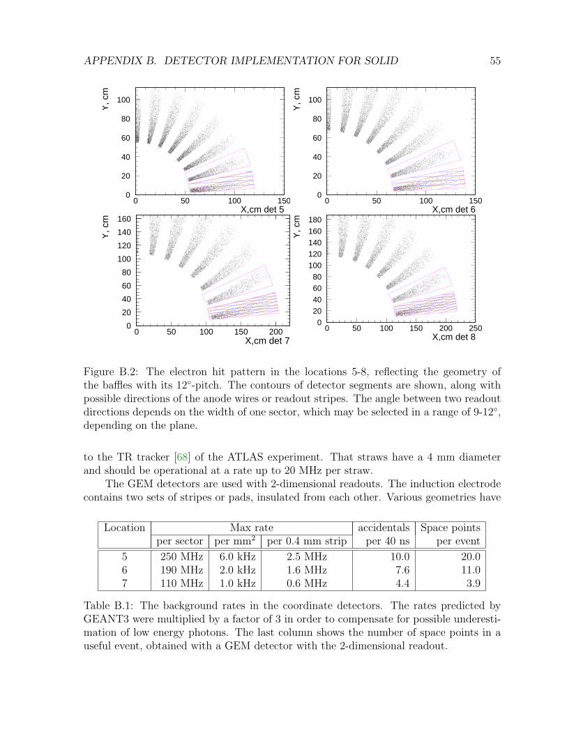
APPENDIX B. DETECTOR IMPLEMENTATION FOR SOLID 55
0
20
40
60
80
100
0 50 100 150X,cm det 5
Y, c
m
0
20
40
60
80
100
0 50 100 150X,cm det 6
Y, c
m
0
20
40
60
80
100
120
140
160
0 50 100 150 200X,cm det 7
Y, c
m
020406080
100120140160180
0 50 100 150 200 250X,cm det 8
Y, c
m
Figure B.2: The electron hit pattern in the locations 5-8, reflecting the geometry ofthe baffles with its 12-pitch. The contours of detector segments are shown, along withpossible directions of the anode wires or readout stripes. The angle between two readoutdirections depends on the width of one sector, which may be selected in a range of 9-12,depending on the plane.
to the TR tracker [68] of the ATLAS experiment. That straws have a 4 mm diameterand should be operational at a rate up to 20 MHz per straw.
The GEM detectors are used with 2-dimensional readouts. The induction electrodecontains two sets of stripes or pads, insulated from each other. Various geometries have
Location Max rate accidentals Space pointsper sector per mm2 per 0.4 mm strip per 40 ns per event
5 250 MHz 6.0 kHz 2.5 MHz 10.0 20.06 190 MHz 2.0 kHz 1.6 MHz 7.6 11.07 110 MHz 1.0 kHz 0.6 MHz 4.4 3.9
Table B.1: The background rates in the coordinate detectors. The rates predicted byGEANT3 were multiplied by a factor of 3 in order to compensate for possible underesti-mation of low energy photons. The last column shows the number of space points in auseful event, obtained with a GEM detector with the 2-dimensional readout.

APPENDIX B. DETECTOR IMPLEMENTATION FOR SOLID 56
been tested, with the angle between the stripes (U-V) from 5 [69] to 90 [54]. Theamplitude correlation of the signals from the two planes can suppress the false U-Vcombinations by a factor of ∼5, reducing the number of planes and projections neededfor the pattern recognition.
Assuming that each of 4 detector planes consists of 30 GEM sectors 10 wide, withstripes made along the sector sides (see Fig. B.2), we end up with a stereo angle of 10.
Table B.1 indicates that the pattern recognition would start with about 850 potentialtrajectories - combinations of space points in 3 planes. Due to a weak dependence of thebackground distribution with the radius, we assume that the detector plane is uniformlypopulated with false spatial points. Just considering the radial coordinates: the plane8 (or 7) 100 cm long radially is close to the calorimeter with a 1 cm radial resolution.This suppresses the 3.9 false hit per good event by a factor of 100. For each hit in plane8 only a band 8 cm wide in radius in plane 6 can contain the matching hit, due to thetarget size. This leaves about 10% of the track candidates, namely 0.1·11=1.1 false trackper event. Then, the matching to plane 5 can be done in a road better than 3 mm wide,which leaves about 0.06 of false tracks per event. The matching in ϕ as well as the energymatching with the calorimeter should further reduce this contamination. A 4-th plane,at the location close to the plane 5, would reduce the false tracks by a factor of 0.06. Anadditional reduction of the false space hits in one plane can be potentially achieved byusing signals from the last GEM, properly segmented1.
Sector TotalLocation Z # ∆ϕ Rmin Rmax pitch # surface #
cm cm cm mm chan m2 chan
5 155 30 10 55 115 0.4 1000 2.7 30 k6 185 30 10 65 140 0.4 1220 4.0 36 k7 295 30 10 105 200 0.6 1160 7.6 35 k8 310 30 10 115 215 0.6 1250 8.6 38 k
total 23.0 140 k
Table B.2: The sizes and the number of readout channels in the GEM coordinate detec-tors.
Let us assume all the detectors are built using the GEM technology, similar to [53,54],but with a smaller angle of ∼ 10 between the readout projections. The readout pitchwas 0.4 mm and a resolution of 71 µm was achieved. Although a resolution of 200 µm issufficient for us, increasing the pitch increases the rate per stripe, therefore we considerthe same 0.4 mm pitch for the planes 5 and 6 and a wider pitch of 0.6 mm for the planes7 and 8. The detector sizes and the numbers of channels are given in Table B.2.
Several potential issues with the GEM detectors may occur and need to be consideredat the stage of further optimization. The largest working chambers so far have a size of
1 This technique is being developed for the Super Big Bite project at JLab
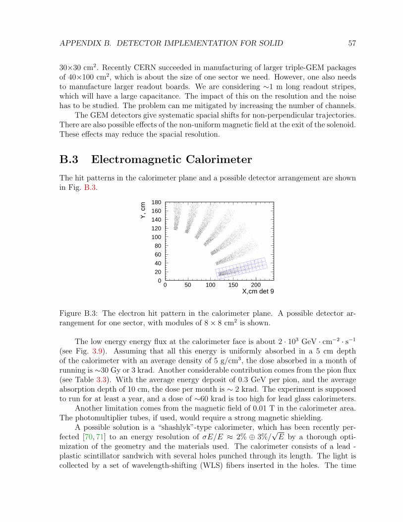
APPENDIX B. DETECTOR IMPLEMENTATION FOR SOLID 57
30×30 cm2. Recently CERN succeeded in manufacturing of larger triple-GEM packagesof 40×100 cm2, which is about the size of one sector we need. However, one also needsto manufacture larger readout boards. We are considering ∼1 m long readout stripes,which will have a large capacitance. The impact of this on the resolution and the noisehas to be studied. The problem can me mitigated by increasing the number of channels.
The GEM detectors give systematic spacial shifts for non-perpendicular trajectories.There are also possible effects of the non-uniform magnetic field at the exit of the solenoid.These effects may reduce the spacial resolution.
B.3 Electromagnetic Calorimeter
The hit patterns in the calorimeter plane and a possible detector arrangement are shownin Fig. B.3.
0
20
40
60
80
100
120
140
160
180
0 50 100 150 200X,cm det 9
Y, c
m
Figure B.3: The electron hit pattern in the calorimeter plane. A possible detector ar-rangement for one sector, with modules of 8× 8 cm2 is shown.
The low energy energy flux at the calorimeter face is about 2 · 103 GeV · cm−2 · s−1
(see Fig. 3.9). Assuming that all this energy is uniformly absorbed in a 5 cm depthof the calorimeter with an average density of 5 g/cm3, the dose absorbed in a month ofrunning is ∼30 Gy or 3 krad. Another considerable contribution comes from the pion flux(see Table 3.3). With the average energy deposit of 0.3 GeV per pion, and the averageabsorption depth of 10 cm, the dose per month is ∼ 2 krad. The experiment is supposedto run for at least a year, and a dose of ∼60 krad is too high for lead glass calorimeters.
Another limitation comes from the magnetic field of 0.01 T in the calorimeter area.The photomultiplier tubes, if used, would require a strong magnetic shielding.
A possible solution is a “shashlyk”-type calorimeter, which has been recently per-fected [70, 71] to an energy resolution of σE/E ≈ 2% ⊕ 3%/
√E by a thorough opti-
mization of the geometry and the materials used. The calorimeter consists of a lead -plastic scintillator sandwich with several holes punched through its length. The light iscollected by a set of wavelength-shifting (WLS) fibers inserted in the holes. The time
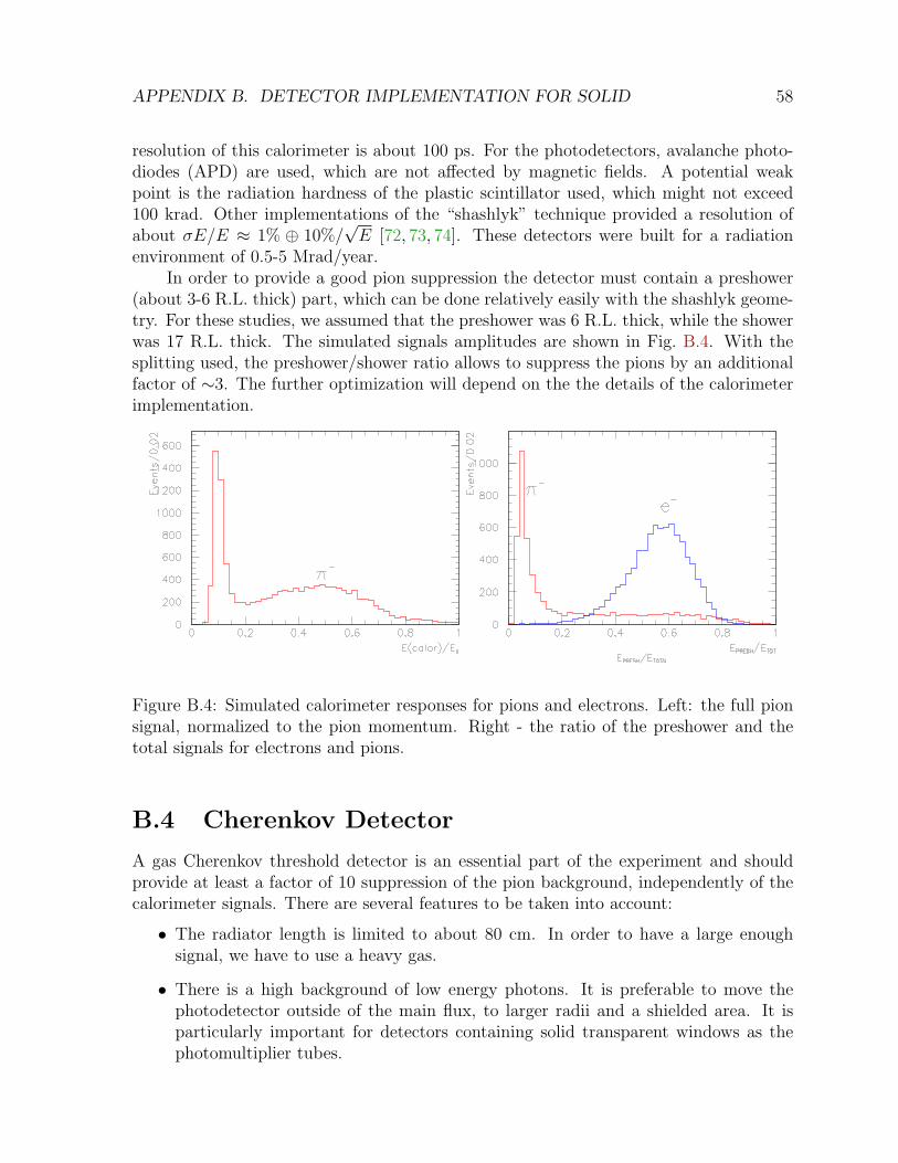
APPENDIX B. DETECTOR IMPLEMENTATION FOR SOLID 58
resolution of this calorimeter is about 100 ps. For the photodetectors, avalanche photo-diodes (APD) are used, which are not affected by magnetic fields. A potential weakpoint is the radiation hardness of the plastic scintillator used, which might not exceed100 krad. Other implementations of the “shashlyk” technique provided a resolution ofabout σE/E ≈ 1% ⊕ 10%/
√E [72, 73, 74]. These detectors were built for a radiation
environment of 0.5-5 Mrad/year.In order to provide a good pion suppression the detector must contain a preshower
(about 3-6 R.L. thick) part, which can be done relatively easily with the shashlyk geome-try. For these studies, we assumed that the preshower was 6 R.L. thick, while the showerwas 17 R.L. thick. The simulated signals amplitudes are shown in Fig. B.4. With thesplitting used, the preshower/shower ratio allows to suppress the pions by an additionalfactor of ∼3. The further optimization will depend on the the details of the calorimeterimplementation.
Figure B.4: Simulated calorimeter responses for pions and electrons. Left: the full pionsignal, normalized to the pion momentum. Right - the ratio of the preshower and thetotal signals for electrons and pions.
B.4 Cherenkov Detector
A gas Cherenkov threshold detector is an essential part of the experiment and shouldprovide at least a factor of 10 suppression of the pion background, independently of thecalorimeter signals. There are several features to be taken into account:
• The radiator length is limited to about 80 cm. In order to have a large enoughsignal, we have to use a heavy gas.
• There is a high background of low energy photons. It is preferable to move thephotodetector outside of the main flux, to larger radii and a shielded area. It isparticularly important for detectors containing solid transparent windows as thephotomultiplier tubes.
APPENDIX B. DETECTOR IMPLEMENTATION FOR SOLID 59
• The magnetic field in a particular place at large radii depends on the yoke design.With the present design it is about 0.01 T in the area convenient for positioningthe photodetectors (Fig. 3.3).
The field of 0.01 T can be shielded enough for the regular PMTs used for Cherenkovdetectors. Therefore, we consider the traditional design of gas Cherenkov threshold de-tectors. The volume is split azimuthally into 15 sectors. Each sector contains an ellipticalmirror, a flat mirror and a photodetector. The optical configuration was optimized us-ing GEANT3. The radiator gas C4F10 (the pion threshold is 2.7 GeV/c) would provideat least 20 photoelectrons in a quartz-window PMT. The sight spot diameter is about18 cm, which will require an optical cone to use a regular, 110 mm photocathode diame-ter PMT. A lighter gas CF4 would provide about 9 photoelectrons with a pion thresholdof 4.2 GeV/c. The light spot will be smaller.
One can also consider photodetectors immune to the magnetic field. A promisingphotodetector design, based on the GEM technology [75,76,77], uses CsI photocathodesdeposited either on the chamber window, or on the GEM surface itself. Depending onthe gas used, it can provide a collection efficiency for electrons of 60% or more.
This approach has been used to build a “hadron-blind” detector at PHENIX [75].It is a windowless, proximity-focus Cherenkov detector with a 50-cm long CF4 radiator.A triple-GEM detector is located in the same gas volume, the photocathode is depositedon the 1-st GEM. A mesh in front of the photocathode provides a cleaning electricalfield preventing the electrons produced by ionizing particles to reach the 1-st GEM. Theabsence of windows or mirrors, along with a very good transparency of the gas to theUV light provides a high photoelectron yield of about 36. The readout pads have a sizecomparable with the spot size of the Cherenkov light of 2 cm2. This detector allows tosuppress pions by a factor of 50 at a 90% efficiency for electrons. This design mightbe applicable for the experiment proposed, however we need a 6.5 m2 photodetector -3-times larger than the PHENIX detector. A potential problem is a high rate of softphotons. On the other hand, the 1000 times finer segmentation than in the standardPMT-based detector, may compensate for the higher background.
Another approach would be a replacement of the PMTs by GEM-based photodetec-tors with quartz windows, 20×20 cm2 each.
B.5 Trigger
The trigger logic (see Section 3.2.6) is based on the calorimeter signals. Each of 30sectors will provide a separate trigger. The implementation depends on the electronicsof the calorimeter. The pipeline electronics using Flash ADCs allows to organize thetrigger within the FADC boards, eliminating the need for separate discriminators. Thisapproach is being developed at JLab for the Hall D experiments.
APPENDIX B. DETECTOR IMPLEMENTATION FOR SOLID 60
B.6 Data Acquisition
The DAQ design will be driven by the detector needs, the rates, and the event topology.The events are single-particle events and are about 1 kbyte in size. The maximumtrigger rate for the full detector is 500 kHz. With segmentation of the detector into 30segments, the rates will be ∼16 kHz in each segment, which should be manageable usingthe pipelining approach that is being developed for the 12 GeV era upgrade of CODA.Using 10 Gigabit networks and fast event-building PCs, as well as large disk buffers andfast tape silos, the event-building and writing to tape might be able to take the full datarate; however, it may be necessary to perform some online data reduction as furtherexplained below.
The DAQ will use the standard JLab CODA (CEBAF Online Data Acquisition)package and will capitalize on the new pipelining frontend architecture being developedfor the 12 GeV upgrade which will achieve high rates, up to 200 kHz with virtually zerodeadtime. The higher frontend rate capability is achieved essentially by having very largebuffers at each stage of the pipeline. Given a trigger, one reads out only the segment ofthe pipeline corresponding to that trigger time. The JLab-designed VME-based F1-TDCsand Flash ADCs will be available and will support pipelining. In addition, competitivecommercial TDC and FADC units are expected to come on the market. The JLab-FADC,for example, will be a 250 MHz 12 bit unit. With the development of a programmableinterface to the FPGA firmware on these FADCs, the possibility of a fast and user-programmable trigger is foreseen, which could make the trigger more flexible and cheaper.Note, this FPGA-based trigger may allow a significant data reduction online, for examplethrowing out spurious hits in the tracking chambers.
We may need to build customized electronics on the frontend for the GEM detectors.For example, the readout developed at CERN [54] also used a pipeline approach which iscompatible with the future JLab DAQ design philosophy. An analog application-specificintegrated circuit (ASIC) called the APV25 was used for the CERN GEM detector. Thechip consists of a preamplifier and shaper stage for each of the input channels, whichwas continuously sampled at 40 MHz and written into memory cells. Upon receiving atrigger, the corresponding memory locations were transferred to a FIFO with a maximumtrigger latency of 4µsec before being multiplexed and read by an ADC. We might copythis design for the GEM detectors, with possible modifications to be compatible with thetrigger supervisor. (The trigger supervisor is a custom-made device built by the JLabDAQ group which is an integral part of CODA.)
To take full advantage of faster frond-end readout, the 12 GeV upgrade of CODAplans to use VME64X crates, 10 Gigabit ethernet, and the new Trigger Supervisor thatis being designed by the DAQ group that will support pipelining. The frontend VMEcpus will be fast, multicore, and have Gigabit ethernet, and will have the option of usingembedded Linux.
Some online data reduction may be necessary to reduce the data rate from 500Mbyte/sec to perhaps less than 50 Mbyte/sec. Some reduction of noise and backgroundmay be possible online using the aforementioned FPGA programming in the FADCs. In
APPENDIX B. DETECTOR IMPLEMENTATION FOR SOLID 61
addition, the trigger supervisor supports second-level triggers; the first-level trigger is afast decision and a second-level trigger is a slower, more complex decision, e.g. a decisionthat the event is a pion. The trigger supervisor then flags the data in the pipeline tonot be read out. Further online reduction is possible in either the VME cpus or in theevent-builder workstations where even more complex decisions can be made based onanalysis of the data. Our preliminary plan is to analyze all the events on-line and writeout the raw data only for about 10% of events, for calibration and monitoring purposes.
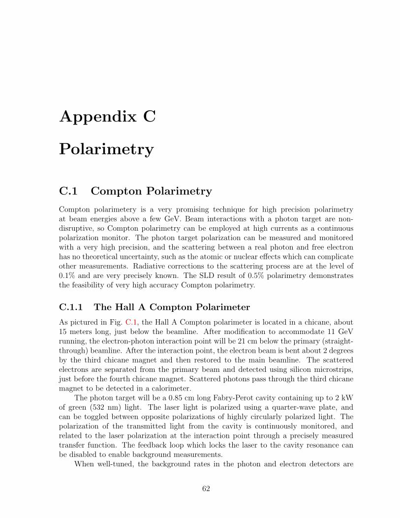
Appendix C
Polarimetry
C.1 Compton Polarimetry
Compton polarimetery is a very promising technique for high precision polarimetryat beam energies above a few GeV. Beam interactions with a photon target are non-disruptive, so Compton polarimetry can be employed at high currents as a continuouspolarization monitor. The photon target polarization can be measured and monitoredwith a very high precision, and the scattering between a real photon and free electronhas no theoretical uncertainty, such as the atomic or nuclear effects which can complicateother measurements. Radiative corrections to the scattering process are at the level of0.1% and are very precisely known. The SLD result of 0.5% polarimetry demonstratesthe feasibility of very high accuracy Compton polarimetry.
C.1.1 The Hall A Compton Polarimeter
As pictured in Fig. C.1, the Hall A Compton polarimeter is located in a chicane, about15 meters long, just below the beamline. After modification to accommodate 11 GeVrunning, the electron-photon interaction point will be 21 cm below the primary (straight-through) beamline. After the interaction point, the electron beam is bent about 2 degreesby the third chicane magnet and then restored to the main beamline. The scatteredelectrons are separated from the primary beam and detected using silicon microstrips,just before the fourth chicane magnet. Scattered photons pass through the third chicanemagnet to be detected in a calorimeter.
The photon target will be a 0.85 cm long Fabry-Perot cavity containing up to 2 kWof green (532 nm) light. The laser light is polarized using a quarter-wave plate, andcan be toggled between opposite polarizations of highly circularly polarized light. Thepolarization of the transmitted light from the cavity is continuously monitored, andrelated to the laser polarization at the interaction point through a precisely measuredtransfer function. The feedback loop which locks the laser to the cavity resonance canbe disabled to enable background measurements.
When well-tuned, the background rates in the photon and electron detectors are
62
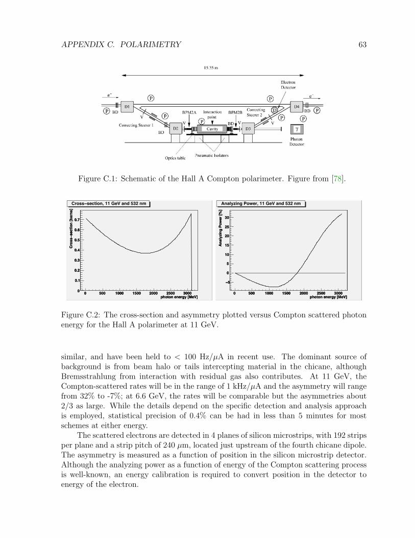
APPENDIX C. POLARIMETRY 63
Figure C.1: Schematic of the Hall A Compton polarimeter. Figure from [78].
photon energy [MeV]0 500 1000 1500 2000 2500 3000
Cro
ss−s
ectio
n [b
arns
]
0
0.1
0.2
0.3
0.4
0.5
0.6
0.7
Cross−section, 11 GeV and 532 nm
photon energy [MeV]0 500 1000 1500 2000 2500 3000
Cro
ss−s
ectio
n [b
arns
]
0
0.1
0.2
0.3
0.4
0.5
0.6
0.7
photon energy [MeV]0 500 1000 1500 2000 2500 3000
Ana
lyzi
ng P
ower
[%]
−5
0
5
10
15
20
25
30
Analyzing Power, 11 GeV and 532 nm
photon energy [MeV]0 500 1000 1500 2000 2500 3000
Ana
lyzi
ng P
ower
[%]
−5
0
5
10
15
20
25
30
Figure C.2: The cross-section and asymmetry plotted versus Compton scattered photonenergy for the Hall A polarimeter at 11 GeV.
similar, and have been held to < 100 Hz/µA in recent use. The dominant source ofbackground is from beam halo or tails intercepting material in the chicane, althoughBremsstrahlung from interaction with residual gas also contributes. At 11 GeV, theCompton-scattered rates will be in the range of 1 kHz/µA and the asymmetry will rangefrom 32% to -7%; at 6.6 GeV, the rates will be comparable but the asymmetries about2/3 as large. While the details depend on the specific detection and analysis approachis employed, statistical precision of 0.4% can be had in less than 5 minutes for mostschemes at either energy.
The scattered electrons are detected in 4 planes of silicon microstrips, with 192 stripsper plane and a strip pitch of 240 µm, located just upstream of the fourth chicane dipole.The asymmetry is measured as a function of position in the silicon microstrip detector.Although the analyzing power as a function of energy of the Compton scattering processis well-known, an energy calibration is required to convert position in the detector toenergy of the electron.
APPENDIX C. POLARIMETRY 64
The calorimeter for detecting scattered photons lies about 7 meters downstream ofthe interaction point. The strong forward boost of scattered photons leads to a tightlycollimated photon beam (< 1 mrad), so the calorimeter size relates only to energy resolu-tion through shower loss. The detector response function is calibrated using the electrondetector to tag the photon energy. This response function is convoluted with the expectedasymmetry distribution to estimate the analyzing power.
The specific calorimeter to be employed is not yet determined. Hall A has used alead tungstate array at higher (> 3 GeV) energies. Althought the light yield is low, thisis not an issue for higher photon energies of the measurements planned here, and thehigh speed of this material reduces pile-up issues. At lower energies, Hall A will use aGSO crystal with much higher light yield. This crystal might also be suitable, but it issomewhat slower than the lead tungstate. Designs for multi-layer sampling calorimeters,using either scintillation or Cerenkov light, will also be considered.
C.1.2 Systematic Uncertainties
Although the electron and photon detectors measure the same scattering events, many ofthe potential systematic errors arise in detector calibration and are entirely decorrelatedbetween the analyses. Other sources of error, especially those that are related to thescattering process such as photon polarization or the total luminosity, are fully correlatedbetween the two systems. Each of these separate catagories of potential systematicuncertainty: correlated, electron-only, and photon-only, will be discussed in the followingsections.
Sources of Correlated Error
Any error associated with the Compton scattering process will be a common source ofsystematic error between the electron- and photon-detector analyses. One example liesin the energy normalization of the scattering process. The analyzing power is a functionof both electron energy and photon energy, so these must be precisely determined. Thephoton wavelength will be determined to better than 0.1 nm and the electron energy to5× 10−4, which leads to an uncertainty at the level of 0.03%.
A more significant source of error comes from the uncertainty in the photon polar-ization. The laser polarization at the interaction point is measured directly by openingthe vacuum chamber and inserting optical diagnostics. The cavity mirrors must be re-moved for this measurement, as they do not transmit sufficient light for measurementwhen the cavity is not resonant. The effect of the mirrors is deduced from the changein the transfer function through the cavity, after the mirrors are replaced and the cavitylocked. This effect is small, typically less than 0.1%. The polariation of the transmittedbeam is monitored during production running. In the present Hall A polarimeter, theuncertainty in beam polarization is estimated at 0.35%. Although this number seemsquite small, it should be kept in mind that it combines two relatively less challengingmeasurements: a measure of the depolarization and the linear polarization of the laserlight at the level of 8%.
APPENDIX C. POLARIMETRY 65
This result can be improved. More frequent measurement of the polarization andmonitoring will be required, and a more sophisticated monitoring scheme will be imple-mented. The effect of vacuum windows will be studied, and if determined to be signif-icant, the strain of the window under vacuum will be included in the transfer functionmeasurement. The circular polarization is near maximum, so the sensitivity to addi-tional birefringence is low. With the necessary effort, the circular polarization of thelaser will be known with a precision of not less than 0.2%, which represents an error inthe combined linear polarization and depolarization of not worse than 4.5%.
Helicity-correlated changes in luminosity of the laser/electron interaction point canintroduce a false asymmetry. Various causes of luminosity variation must be consid-ered, such as electron beam intensity, beam motion or spot-size variation. The controlof helicity-correlated beam asymmetries is now a standard technology at Jefferson Lab,and typically achievable results (few part per million intensity, 10’s of nanometers beammotion, < 10−3 spot size changes) will suitably constrain the electron-photon crossingluminosity variations. Another possible source of false asymmetry would be electron-ics pickup of the helicity signal, which could potentially impact an integrating photonanalysis. However, the demands of the primary experiment for isolation of the helicitysignal exceed those for polarimetry by several orders of magnitude. In addition, the laserpolarization reversal provides an additional cancellation for asymmetries correlated tothe electron beam helicity. Potential effects must be carefully considered, but with dueeffort, false asymmetries will be a negligible source of uncertainty in this measurement.
Backgrounds are a common, though not fully correlated, problem for the two detectorsystems. The Hall A polarimeter commonly runs with a signal to background ratio ofaround 10:1. All known backgrounds are related only to the electron beam, and are notcorrelated to the presence of the laser light. Frequent, precise background measurementscan be easily made by turning off the laser power. As a matter of routine, between 30-60% of data taking is done without the laser, for the purpose of background subtraction.Direct effects of background asymmetries and dilutions are presently estimated to be lessthan 0.04% in the Hall A system.
Systematic Errors for the Electron Detector
There are two primary sources of potential uncertainty for the electron detector. The firstof these is a scale error in the measurement of asymmetries due to an imperfect deadtimecorrection. The second broadly concerns detector response, spectrometer uniformity andcalibration and the impact on the estimated analyzing power.
With data rates potentially up to 100 kHz, DAQ deadtime corrections will be po-tentially significant, and a dedicated effort to control the related uncertainty will benecessary. The fast-counting DAQ can take very high rates with low deadtimes, and de-terministic deadtime intervals are enforced in readout and acquisition electronics stages.The high statistical power of the measurement is of significant use here; the laser powercan be varied and the effects mapped to a very high degree of statistical precision. Thepotential systematic error from deadtime correction arises from asymmetry deadtime as-
APPENDIX C. POLARIMETRY 66
sociated with the total counting asymmetry. Although the peak asymmetry is high, thetotal integrated asymmetry is considerably reduced by the accepted range of negativeasymmetry. With care, the total asymmetric deadtime correction will introduce no morethan 0.2% uncertainty in the determination of polarization.
The analyzing power for the measured electron distribution can be very accuratelydetermined. The calibration is assisted by the accessibility of two easily identified pointsof well-defined kinematics: the Compton edge and the asymmetry zero-crossing (0-Xing).Both points are fully determined by the beam and photon energies, and provide a precisemethod for energy calibration of the electron spectrum. The asymmetry spectrum for11 GeV is plotted in Figure C.2. At 11 GeV, the Compton edge is 3.1 GeV below thebeam momentum, with a peak asymmetry of ∼ 32%, and 0-Xing is 1.8 GeV below beammomentum. At the detector, these are located about 4.7 and 2.7 cm from the primarybeam, respectively. At 6.6 GeV, the 1.26 GeV Compton edge is 3.2 cm from the primarybeam with an asymmetry of ∼ 20.8%, while the zero-crossing at 700 MeV below beamenergy is 1.8 cm from the beam.
The dominant uncertainties in this method involve the location of these points in thedetector and the knowledge of the detector response between the end points. Dependingon the analysis method, one can be variously sensitive or insensitive to these uncertainties.Here, we consider three separate methods for analyzing the electron detector data.
• Integration The polarization can be determined as a counting asymmetry for thesum of all strips from the Compton edge to the zero crossing.
Since there is no Compton-scatter rate above the Compton edge, there is no sys-tematic uncertainty in the analyzing power related to the estimated location of thispoint. The high momentum side of the integration cutoff will not occur preciselyat the 0-Xing, but rather at an electron energy corresponding to as much as ±0.5of the pitch of the silicon detector strips. Since the asymmetry near the 0-Xingis nearly zero, the error in the 0-Xing location reduces the estimated analyzingpower proportionally to the associated fractional change in expected rate; this iseffectively an error in background dilution.
The location of the 0-Xing will be fit using the nearly linear shape of the nearbyasymmetry distribution. This procedure will introduce an additional source ofstatistical noise in the determination of the electron polarization. Small variationsin the beam deflection by the third dipole and in the location of the electron detectorwill reduce systematic bias from the discretization of the data into the silicon strips,or from local differences in efficiency. It should be possible to avoid a systematicbias to a level better than 5% of the width of a strip, which would correspond to a0.06% effect at 11 GeV and an 0.1% effect at 6 GeV.
An error in the 0-Xing location could also arise from an experimental false asym-metry. The slope near the 0-Xing is such that a 0.1% false asymmetry would resultin reduction of 0.25% the estimated analyzing power (and so a +0.25% in the mea-sured electron polarization). The false asymmetry would directly represent an errorin the electron polarization of about 0.51%, so this effect increases the sensitivity
APPENDIX C. POLARIMETRY 67
to false asymmetry by factor of about 1.5. Even with this enhancement, the falseasymmetry contribution to the polarization will still be negligible.
Probably the most significant uncertainty in the analyzing power will arise fromefficiency variations among the silicon strips. Strip-by-strip efficiencies can be calcu-lated by comparing track-hit efficiency between the 4 planes of the silicon detector.Inefficiency is expected to be low (less than 1%) and well measured, which willhelp minimize this effect. Comparison of results from the 4 detector planes willprovide a cross-check on this effect, since local variations in asymmetries shouldbe independent between the planes. Significant variations in the location of thedetector relative to the primary beam, which would also help control this effect,should be possible, depending on the observed beam halo.
• Asymmetry Fit The polarization can also be found from the shape of the asymme-try over all strips between the Compton edge and the zero crossing. This techniquewould share the small uncertainties on determination of the 0-Xing with the inte-gration technique. However, it would not be sensitive to strip-to-strip variations inefficiency, which is the dominant senstivity for the integration technique.
This fit would be senstive to knowledge of the magnetic field uniformity. Deviationsfrom the expected shape would introduce systematic uncertainty. Such an an effectmay be evident in fit χ2, could be cross-checked against the rate distribution, andcould also be studied in high-statistics electron asymmetry distribution averagedover many runs.
• Single Strip The statistical power of the last, single silicon strip at the Comptonedge will be significant, capable of 0.5% measurements on time-scales of around 15minutes at 11 GeV or 20 minutes at 6.6 GeV. The rate of change of the asymmetryin this region is only 0.9% / mm. Locating this strip, relative to Compton edge,to a little better than half its own width should provide a robust 0.1% accuracy onthe analyzing power. This technique would have a greatly reduced sensitivity tothe 0-Xing location, dispersion variations or strip efficiency.
For each of these techniques the analyzing power should be estimated with an accuracyof around 0.2% or better. The cross-checks between techniques, each of which have verydifferent sensitivities to possible sources of error, will provide convincing evidence that thesystem is well understood. Given these considerations, it seems likely that the electrondetector analyzing power will not be the dominant source of systematic uncertainty forthe polarimetry analysis.
Systematic Errors for the Photon Detector
The determination of the analyzing power is more difficult for the photon calorimeterthan for the electron detector due to the width, and shape, of the detector responsefunction. The photon detector analyzing power calculation must convolute this responsefunction with the theoretical analyzing power curve. The response function shape and

APPENDIX C. POLARIMETRY 68
energy calibration can be studied using the photon tagging through coincidence triggerswith the electron detector.
In general, determining the effect of a low-energy threshold on the analyzing powerdepends sensitively on the shape of the response function; at low energies this is a majorsource of uncertainty. At high energies, the improved resolution and consistency of theresponse function shape over the range of interest will significantly reduce this problem.The electron-tagged photon spectrum, which can be calibrated to the zero-crossing andcompton edge of the electron spectrum, is crucial to the energy calibration of the photondetector. The optimum location for the low-energy threshold is likely the asymmetryminimum, where uncertainty in the threshold will have minimal effect. Verifing thatthe electron polariazation result remains constant over variations in the applied lowerthreshold of the asymmetry analysis provides a useful cross-check of the technique.
Uncertainties related to the threshold, response function shape, and absolute energycalibration can also be eliminated by integrating all signal, without threshold. Theseprevious problems are then replaced with a requirement on the uniformity of the aver-age response over photon energy. At high energies, one expects very uniform behavior,although detector linearity will be crucial. Because the analyzing power integral is energy-weighted, the statistical figure-of-merit is not badly degraded by the negative asymmetryregion.
The PREX experiment, with a beam energy of 1.2 GeV, will be unable to detect theasymmetry zero-crossing in the electron detector and so will be relying on the integratingphoton method for polarimetry at the level of 1% precision. Complications in the responsefunction for few to 10 MeV photons, and the inability to detect the electrons to tagelectrons of such low energy, make that low energy experiment very challenging. Suchlow energy photons will be only a small correction to the result at 6.6 or 11 GeV. With theability to study response function with the tagged photon beam over most of the energyrange, the photon detector analyzing power normalization in the range of 0.3-0.4% shouldbe achievable.
The rate in the photon detector is similar to that in the electron detector, around1 kHz/µA, and the deadtime correction represents a similar potential systematic un-certainty. Counting in the photon detector is also senstive to pile-up, which distortsthe asymmetry distribution. Background and rate distributions will serve as inputs tosimulation for corrections on the analyzing power determination. In the current Hall Aanalysis, pile-up effects are estimated at the level of 1%, and the effect can be controledat a level better than 10% of itself. An integrating photon analysis requires no dead-time correction and has a greatly reduced sensitivity to pile-up, which is a significantadvantage for high precision.
C.1.3 Summary of Compton Polarimetry Uncertainties
The prospects for 0.4% Compton polarimetry are excellent. However, an extremelyaggressive and dedicated effort to reducing systematic uncertainty will be required. Ta-ble C.1.3 summarizes the systematic uncertainty estimates discussed above.

APPENDIX C. POLARIMETRY 69
Relative error (%) electron photon
EBeam 0.03 0.03Laser polarization 0.20 0.20False asymetries 0.01 0.01Background 0.05 0.05Deadtime 0.2 0.0Pileup 0.0 0.1Analyzing power 0.2 0.40
Total: 0.35 0.46
Table C.1: Table of systematic uncertainties for the Hall A Compton polarimeter at6.6 GeV and 11 GeV. Estimates are described in Sect. C.1.2.
These ambitious goals will require vigorous and dedicated efforts to reduce sourcesof systematic uncertainty. It is expected that some significant fraction of data produc-tion time will be used for studies of the Compton polarimeter system which are notdisruptive to the experiment, for example, scans of detector positions, laser power andpolarization, data acquisition parameters, etc. The scattering asymmetry with both the6.6 and 11 GeV beams is relatively large, which allows precision at the level of ∼0.5%in less than 1 minute of data. Given this high statistical power, these studies will be aneffective method for constraining many of the possible experimental systematic uncer-tainties.
The future use of the Hall A polarimeter at 6.6 and 11 GeV will be a very differentsituation from the recent operation. The dominant systematic error in recent operationlay in the determination of the analyzing power. Operating at lower energies, and withan infrared (1064 nm) laser, the asymmetries were significantly lower and therefore thestatistical power was worse. In addition, the limits of systematic uncertainty had notbeen pushed by demands of the experiment precision.
In the case of previous analyses of the electron detector, the zero-crossing calibrationhad not been exploited. The 0-Xing “integration” analysis was attempted for the firsttime for the HAPPEX-II and HAPPEX-He measurements. The situation was compli-cated due to the low beam energy of around 3 GeV, which not only reduced the averageasymmetry but also reduced the ratio of Compton-scattered photon energies and theelectron energies. At 3 GeV, the zero-crossing was about 5 mm from the primary beam,which was as close as the electron detector could get to the beam. Geometric efficiencyat the edge was a signficant complication in this approach. In addition, the microstripdetector was damaged and displayed low and uneven efficiency, which complicated theanalysis. The estimated systematic errors for that analysis which were not associatedwith these efficiency issues are consistent with Table C.1.3.
For the photon detector, the integration readout method has not yet been usedfor a physics experiment, and the counting photon analysis was typically limited byuncertainties in the detector response at lower energies. And the rapid access to high
APPENDIX C. POLARIMETRY 70
statistical power, which is so powerful for cross-checking potential sources of systematicuncertainty, has never before been available to the Hall A Compton.
High-precision Compton polarimetry has also been widely applied at storage ringsand colliders. Uncertainties in analyzing power determination have typically limited theprecision of high-energy collider Compton photo-detectors to typically ∼ 0.8%. Thesemeasurements typically use the integrating photon technique for production running,since the electron beam currents are so high. However, in these measurements, photontagging through coincidence with an electron detector is typically not available for studyof the detector response function. The ability of the Hall A Compton polarimeter toperform in situ tagged photon calibrations will be a significant advantage.

APPENDIX C. POLARIMETRY 71
C.2 Møller Polarimetry
C.2.1 Møller Scattering
Møller polarimeters exploit the properties of the polarized Møller scattering ~e− + ~e− →e− + e−. Its unpolarized cross section, first calculated by C. Møller [79], in the Bornapproximation and the ultrarelativistic limit depends on the scattering angle in c.m.Θcm and the Mandelstam variable s as:
dσdΩcm
=α2
s· (4− sin2 Θcm)2
sin4 Θcm
, (C.1)
where α is the electomagnetic coupling constant, also presentable as α = re ·me, wherere = 2.817 · 10−13 cm is the classical electron radius. In the lab frame of the fixed targetexperiments, the scattering cross section at Θcm = 90 does not depend on s:
dσdΩ
(Θcm = 90) ≈ 178 mb/ster. (C.2)
The polarized cross section depends on the beam and target polarizations Pbeam andPtarget as:
dσ
dΩcm
=dσdΩcm
· (1 +∑
i=X,Y,Z
(AMii · Ptarg i · Pbeam i)), (C.3)
where i = X, Y, Z defines the projections of the polarizations. The analyzing power AM ,calculated in the same limits as Eq. C.1 [80, 81], depends on the angle Θcm and doesnot depend on s. Assuming that the beam direction is along the Z-axis and that thescattering happens in the ZX plane:
AMZZ = −sin2 Θcm · (7 + cos2 Θcm)
(3 + cos2 Θcm)2, AM
XX = − sin4 Θcm
(3 + cos2 Θcm)2, AM
Y Y = −AMXX (C.4)
At Θcm = 90o the analyzing power has its maximum AMZZ max = 7/9. A beam transverse
polarization in the scattering plane also leads to an asymmetry, though the analyzingpower is lower: AM
XX max = AMZZ/7. The main purpose of the polarimeter is to measure
the longitudinal component of the beam polarization.
C.2.2 Ways to Higher Accuracy
The polarized Møller scattering (described in Section C.2.1) is a convenient process formeasuring the beam polarization. Its counting rate does not depend on the energy, theanalyzing power is high (about 80%) and neither depends on the energy, nor changes con-siderably in the range of the polarimeter acceptance, and two electrons with high energiesin the final state make it easy to detect their coincidence and reduce the background tonegligible values.
For the polarized electron target only ferromagnetic foils have been used so far[82, 83, 84, 85, 86, 87, 88]. In fully magnetized iron, for instance, about 2.1 electrons from
APPENDIX C. POLARIMETRY 72
the d-shell are polarized and the average electron polarization is about 8%. This valuecan not be calculated from the first principles, but has to be derived from the measuredmagnetization. Most of the polarimeters used foils tilted at an angle of about 20 to thebeam and magnetized by external fields of 10-30 mT directed along the beam. In theseconditions the magnetization is not fully saturated and depends on many parametersincluding the foil annealing and history. It can be measured, typically with an accuracyof 2-3%. The polarimeter of Hall C at JLab [89,88] uses foils perpendicular to the beam,magnetized to full saturation in a strong longitudinal field of 3-4 T. In this case, themagnetization has not been measured, but taken from published data on the propertiesof bulk iron, which claims an accuracy of ∼ 0.1%. In both cases, the orbital contributionto the magnetization of about 5% can be evaluated and subtracted using the magneto-mechanical factor, measured by other dedicated experiments [90]. With strong externalfields of 3-4 T several additional correction of about 0.5% have to be made to compensatefor extra orbital momenta and other complex effects. This correction is temperaturedependent.
The magnetization of ferromagnetics depends on the temperature. The beam heatsup the foil and the temperature in the beam area is difficult to measure or calculateaccurately. This limits the average beam current to 2-3 µA, much lower than the currentof> 50 µA to be used in the experiment. Using different beam regimes for experiment andpolarimetry may become a source of systematic errors, difficult to evaluate. A possibleway to solve this problem is to use a fast “kicker” magnet to move the beam back andforth across the edge of a foil located at a distance of about 1 mm from the regular beamposition [91].
Another source of errors is the heavy atom used for the target. Møller scatteringoff electrons from the internal atomic shells has a distorted energy-angle correlation ofthe secondary electrons, with respect to scattering off electrons from the external shells.A difference of the polarimeter acceptance to these two classes of events is the sourceof a systematic bias (so-called Levchuk effect [92]), typically of about 1-5%. This effectforbids using a strong optical collimation of the secondary particles, favorable otherwisefor background suppression. In most cases, the background is dominated by electron-nucleus scattering and contains one electron in the final state. It can be efficientlysuppressed by detecting both secondary Møller electrons in coincidence, however thisbackground typically doubles the detectors’ counting rate.
The counting rates depend on the target thickness and the apparatus acceptance.The acceptance should not be too small, because of the Levchuk effect. The associateddead time is typically not negligible and can be a source systematic errors.
The list of systematic errors for the JLab Møller polarimeters in Hall A and Hall Care presented in Table C.2.
Although it is possible to reduce considerably the systematic error of the foil polar-ization by using a very high magnetization field [88], it is difficult to reduce the othererrors, in particular the one associated with the beam current limitations. Also, it isdifficult to organize continuous measurements since even the thinnest foil used (∼ 1 µm)
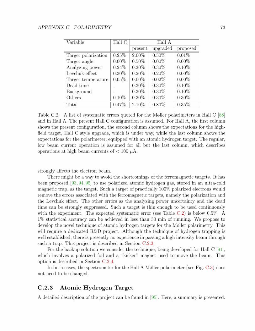
APPENDIX C. POLARIMETRY 73
Variable Hall C Hall Apresent upgraded proposed
Target polarization 0.25% 2.00% 0.50% 0.01%Target angle 0.00% 0.50% 0.00% 0.00%Analyzing power 0.24% 0.30% 0.30% 0.10%Levchuk effect 0.30% 0.20% 0.20% 0.00%Target temperature 0.05% 0.00% 0.02% 0.00%Dead time - 0.30% 0.30% 0.10%Background - 0.30% 0.30% 0.10%Others 0.10% 0.30% 0.30% 0.30%
Total 0.47% 2.10% 0.80% 0.35%
Table C.2: A list of systematic errors quoted for the Møller polarimeters in Hall C [88]and in Hall A. The present Hall C configuration is assumed. For Hall A, the first columnshows the present configuration, the second column shows the expectations for the high-field target, Hall C style upgrade, which is under way, while the last column shows theexpectations for the polarimeter, equipped with an atomic hydrogen target. The regular,low beam current operation is assumed for all but the last column, which describesoperations at high beam currents of < 100 µA.
strongly affects the electron beam.There might be a way to avoid the shortcomings of the ferromagnetic targets. It has
been proposed [93, 94, 95] to use polarized atomic hydrogen gas, stored in an ultra-coldmagnetic trap, as the target. Such a target of practically 100% polarized electrons wouldremove the errors associated with the ferromagnetic targets, namely the polarization andthe Levchuk effect. The other errors as the analyzing power uncertainty and the deadtime can be strongly suppressed. Such a target is thin enough to be used continuouslywith the experiment. The expected systematic error (see Table C.2) is below 0.5%. A1% statistical accuracy can be achieved in less than 30 min of running. We propose todevelop the novel technique of atomic hydrogen targets for the Møller polarimetry. Thiswill require a dedicated R&D project. Although the technique of hydrogen trapping iswell established, there is presently no experience in passing a high intensity beam throughsuch a trap. This project is described in Section C.2.3.
For the backup solution we consider the technique, being developed for Hall C [91],which involves a polarized foil and a “kicker” magnet used to move the beam. Thisoption is described in Section C.2.4.
In both cases, the spectrometer for the Hall A Møller polarimeter (see Fig. C.3) doesnot need to be changed.
C.2.3 Atomic Hydrogen Target
A detailed description of the project can be found in [95]. Here, a summary is presented.

APPENDIX C. POLARIMETRY 74
-80
-60
-40
-20
0
20
40
0 100 200 300 400 500 600 700 800Z cm
Y cm
(a)
Tar
get
Co
llim
ato
r
Coils Quad 1 Quad 2 Quad 3 Dipole
Detector
non-scatteredbeam
-20
-15
-10
-5
0
5
10
15
20
0 100 200 300 400 500 600 700 800Z cm
X cm
(b)B→
Figure C.3: The layout of the Hall A Møller polarimeter in it present configuration. Theplanned upgrade for 12 GeV includes lifting of the detector box to compensate for asmaller deflection in the dipole.
Hydrogen Atom in Magnetic Field
The magnetic field BS and the hyperfine interaction split the ground state of hydrogeninto four states with different energies. The low energy states are |a〉 = | ↓−↑〉· cos θ−| ↑−↓〉· sin θ and |b〉=| ↓−↓〉, where the first and second (crossed) arrows in the brackets indicatethe electron and proton spin projections on the magnetic field direction. As far as theelectron spin is concerned, state |b〉 is pure, while state |a〉 is a superposition. The mixingangle θ depends on the magnetic field BS and temperature T : tan 2θ ≈ 0.05 T/BS. AtBS =8 T and T = 0.3 K the mixing factor is small: sin θ ≈ 0.003. State |b〉 is 100%polarized. State |a〉 is polarized in the same direction as |b〉 and its polarization differsfrom unity by ∼ 10−5.
Storage Cell
In a magnetic field gradient, a force −∇( ~µH~B), where µH is the atom’s magnetic moment,
separates the lower and the higher energy states. The lower energy states are pulled intothe stronger field, while the higher energy states are repelled from the stronger field. The0.3 K cylindrical storage cell, made usually of pure copper, is located in the bore of asuperconducting ∼8 T solenoid. The polarized hydrogen, consisting of the low energystates, is confined along the cell axis by the magnetic field gradient, and laterally by thewall of the cell (Fig C.4).
At the point of statistical equilibrium, the state population, p follows the Boltzmann
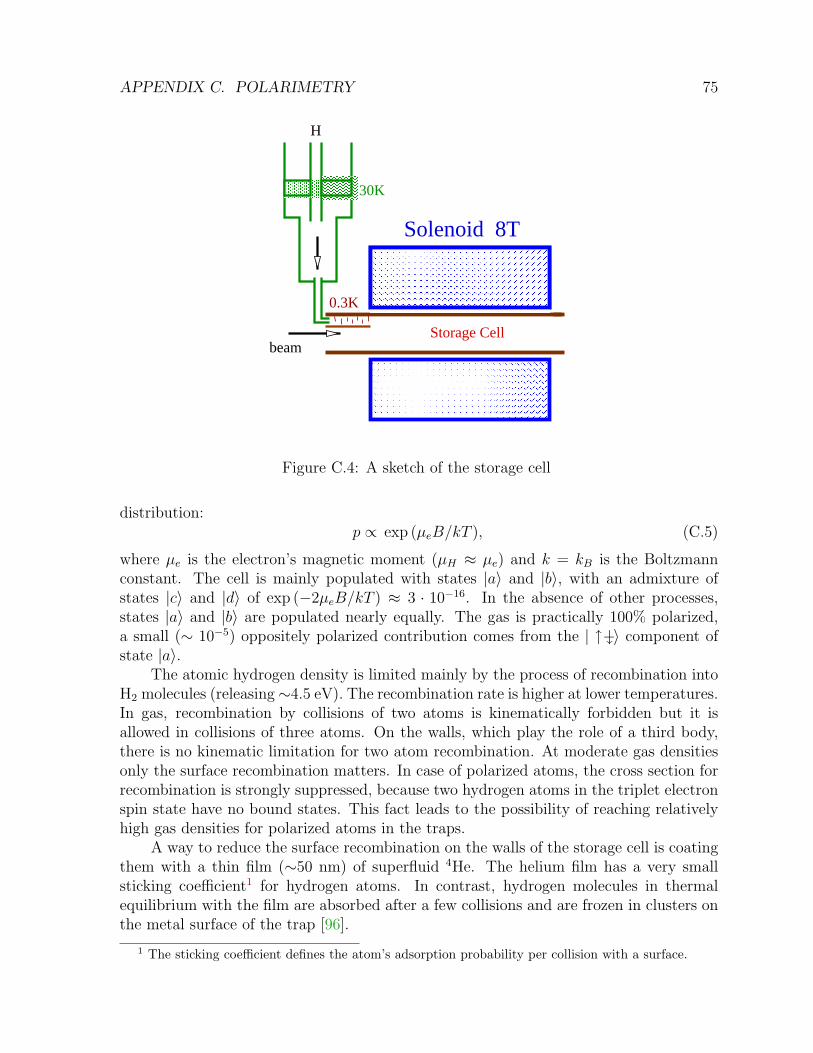
APPENDIX C. POLARIMETRY 75
30K
0.3K
H
Solenoid 8T
beamStorage Cell
Figure C.4: A sketch of the storage cell
distribution:p ∝ exp (µeB/kT ), (C.5)
where µe is the electron’s magnetic moment (µH ≈ µe) and k = kB is the Boltzmannconstant. The cell is mainly populated with states |a〉 and |b〉, with an admixture ofstates |c〉 and |d〉 of exp (−2µeB/kT ) ≈ 3 · 10−16. In the absence of other processes,states |a〉 and |b〉 are populated nearly equally. The gas is practically 100% polarized,a small (∼ 10−5) oppositely polarized contribution comes from the | ↑−↓〉 component ofstate |a〉.
The atomic hydrogen density is limited mainly by the process of recombination intoH2 molecules (releasing∼4.5 eV). The recombination rate is higher at lower temperatures.In gas, recombination by collisions of two atoms is kinematically forbidden but it isallowed in collisions of three atoms. On the walls, which play the role of a third body,there is no kinematic limitation for two atom recombination. At moderate gas densitiesonly the surface recombination matters. In case of polarized atoms, the cross section forrecombination is strongly suppressed, because two hydrogen atoms in the triplet electronspin state have no bound states. This fact leads to the possibility of reaching relativelyhigh gas densities for polarized atoms in the traps.
A way to reduce the surface recombination on the walls of the storage cell is coatingthem with a thin film (∼50 nm) of superfluid 4He. The helium film has a very smallsticking coefficient1 for hydrogen atoms. In contrast, hydrogen molecules in thermalequilibrium with the film are absorbed after a few collisions and are frozen in clusters onthe metal surface of the trap [96].
1 The sticking coefficient defines the atom’s adsorption probability per collision with a surface.
APPENDIX C. POLARIMETRY 76
The higher energy states are repelled from the storage cell by the magnetic fieldgradient and leave the cell. Outside of the helium-covered cell, the atoms promptlyrecombine on surfaces into hydrogen molecules which are either pumped away or arefrozen on the walls. Some of the higher energy states recombine within the cell and themolecules eventually are either frozen on the helium-coated wall, or leave the cell bydiffusion.
The cell is filled with atomic hydrogen from an RF dissociator. Hydrogen, at 80 K,passes through a Teflon2 pipe to a nozzle, which is kept at ∼30 K. From the nozzlehydrogen enters into a system of helium-coated baffles, where it is cooled down to ∼0.3 K.At 30 K and above, the recombination is suppressed because of the high temperature,while at 0.3 K it is suppressed by helium coating. In the input flow, the atoms andmolecules are mixed in comparable amounts, but most of the molecules are frozen out inthe baffles and do not enter the cell.
The gas arrives at the region of a strong field gradient, which separates very efficientlythe lower and higher atomic energy states, therefore a constant feeding of the cell doesnot affect the average electron polarization.
This technique was first successfully applied in 1980 [97], and later a density3 ashigh as 3 · 1017 atoms/cm3 was achieved [98] in a small volume. So far, the storage cellitself has not been put in a high-intensity particle beam.
For the project being discussed a normal storage cell design can be used, with thebeam passing along the solenoid axis (Fig. C.4). The double walls of the cylindricalcopper cell form a dilution refrigerator mixing chamber. The cell is connected to thebeam pipe with no separating windows. The tentative cell parameters are (similar to aworking cell [99]): solenoid maximum field of BS = 8 T , solenoid length of LS = 30 cm,cell internal radius of r = 2 cm, cell length of LC = 35 cm and temperature of T = 0.3 K.The effective length of such a target is about 20 cm.
For the guideline, we will consider a gas density of 3 · 1015 cm−3, obtained experi-mentally [100], for a similar design.
Gas Properties
Important parameters of the target gas are the diffusion speed. At 300 mK the RMSspeed of the atoms is ∼80 m/s. For these studies we used a calculated value [101] of thehydrogen atoms cross section σ = 42.3 · 10−16 cm2, ignoring the difference between thespin triplet and singlet cross sections. This provided the mean free path ` = 0.57 mm atdensity of 3 · 1015 cm−3.
The average time, τd for a “low field seeking” atom to travel to the edge of the cell,assuming its starting point is distributed according to the gas density, is4: τd ≈ 0.7 s.This is the cleaning time for an atom with opposite electron spin, should it emerge in the
2Teflon has a relatively small sticking coefficient for hydrogen atoms.3This parameter is called concentration, but we will use the word density in the text, since the mass
of the gas is not important here.4This time was estimated using simulation, taking into account the gas density distribution along z
and the repelling force in the magnetic field gradient.
APPENDIX C. POLARIMETRY 77
cell and if it does not recombine before. The escape time depends on the initial positionof the atom, going from ∼ 1 s at z = 0 to 0.1 s at z = 8 cm. The average wall collisiontime is about 0.5 ms.
Gas Lifetime in the Cell
For the moment we consider the gas behavior with no beam passing through it. Severalprocesses lead to losses of hydrogen atoms from the cell: thermal escape through themagnetic field gradient, recombination in the volume of gas and recombination on thesurface of the cell.
The volume recombination can be neglected up to densities of ∼ 1017 cm−3 [98].The dominant process, limiting the gas density, is the surface recombination. In
order to keep the gas density constant the losses have to be compensated by constantlyfeeding the cell with atomic hydrogen. Our calculations, based on the theory of suchcells [98], show, that a very moderate feed rate of Φ ∼ 1 · 1015 atoms/s would provide agas density of 7 · 1015 cm−3.
This can be compared with the measurement [100] of 3 · 1015 cm−3. The averagelifetime of a “high field seeking” atom in the cell is ∼1 h.
Unpolarized Contamination
The most important sources of unpolarized contamination in the target gas in absenceof beam have been identified:
1) hydrogen molecules: ∼ 10−5;
2) high energy atomic states |c〉 and |d〉: ∼ 10−5;
3) excited atomic states < 10−10;
4) other gasses, like helium and the residual gas in the cell: ∼ 10−3
The contributions 1)-3) are present when the cell is filled with hydrogen. They are diffi-cult to measure directly and we have to rely on calculations. Nevertheless, the behaviorof such storage cells has been extensively studied and is well understood [98]. The gen-eral parameters, like the gas lifetime, or the gas density are predicted with an accuracybetter than a factor of 3. The estimates 1)-3) are about 100 times below the level ofcontamination of about 0.1% which may become important for polarimetry. In contrast,the contribution 4) can be easily measured with beam by taking an empty target mea-surement. Atomic hydrogen can be completely removed from the cell by heating a smallbolometer inside the cell, which would remove the helium coating on this element, andcatalyze a fast recombination of hydrogen on its surface. However, it is important tokeep this contamination below several percent in order to reduce the systematic errorassociated with the background subtraction.
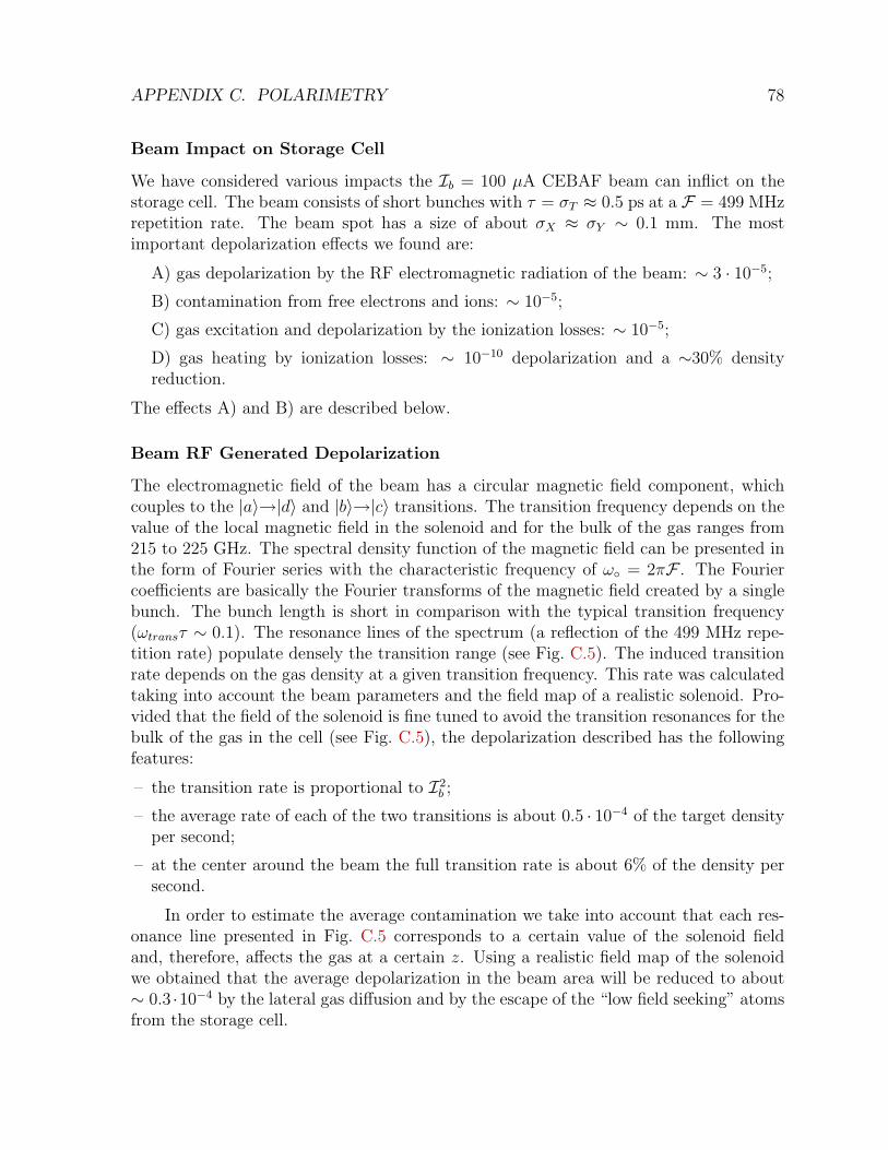
APPENDIX C. POLARIMETRY 78
Beam Impact on Storage Cell
We have considered various impacts the Ib = 100 µA CEBAF beam can inflict on thestorage cell. The beam consists of short bunches with τ = σT ≈ 0.5 ps at a F = 499 MHzrepetition rate. The beam spot has a size of about σX ≈ σY ∼ 0.1 mm. The mostimportant depolarization effects we found are:
A) gas depolarization by the RF electromagnetic radiation of the beam: ∼ 3 · 10−5;
B) contamination from free electrons and ions: ∼ 10−5;
C) gas excitation and depolarization by the ionization losses: ∼ 10−5;
D) gas heating by ionization losses: ∼ 10−10 depolarization and a ∼30% densityreduction.
The effects A) and B) are described below.
Beam RF Generated Depolarization
The electromagnetic field of the beam has a circular magnetic field component, whichcouples to the |a〉→|d〉 and |b〉→|c〉 transitions. The transition frequency depends on thevalue of the local magnetic field in the solenoid and for the bulk of the gas ranges from215 to 225 GHz. The spectral density function of the magnetic field can be presented inthe form of Fourier series with the characteristic frequency of ω = 2πF . The Fouriercoefficients are basically the Fourier transforms of the magnetic field created by a singlebunch. The bunch length is short in comparison with the typical transition frequency(ωtransτ ∼ 0.1). The resonance lines of the spectrum (a reflection of the 499 MHz repe-tition rate) populate densely the transition range (see Fig. C.5). The induced transitionrate depends on the gas density at a given transition frequency. This rate was calculatedtaking into account the beam parameters and the field map of a realistic solenoid. Pro-vided that the field of the solenoid is fine tuned to avoid the transition resonances for thebulk of the gas in the cell (see Fig. C.5), the depolarization described has the followingfeatures:
– the transition rate is proportional to I2b ;
– the average rate of each of the two transitions is about 0.5 · 10−4 of the target densityper second;
– at the center around the beam the full transition rate is about 6% of the density persecond.
In order to estimate the average contamination we take into account that each res-onance line presented in Fig. C.5 corresponds to a certain value of the solenoid fieldand, therefore, affects the gas at a certain z. Using a realistic field map of the solenoidwe obtained that the average depolarization in the beam area will be reduced to about∼ 0.3 ·10−4 by the lateral gas diffusion and by the escape of the “low field seeking” atomsfrom the storage cell.
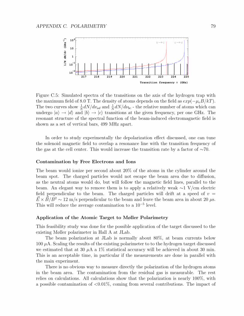
APPENDIX C. POLARIMETRY 79
10-2
10-1
1
10
102
217 218 219 220 221 222 223 224 225
Transition frequency ν (GHz)
1/N dN/d
ν (GHz-1)
Figure C.5: Simulated spectra of the transitions on the axis of the hydrogen trap withthe maximum field of 8.0 T. The density of atoms depends on the field as exp(−µeB/kT ).The two curves show 1
NdN/dνad and 1
NdN/dνbc - the relative number of atoms which can
undergo |a〉 → |d〉 and |b〉 → |c〉 transitions at the given frequency, per one GHz. Theresonant structure of the spectral function of the beam-induced electromagnetic field isshown as a set of vertical bars, 499 MHz apart.
In order to study experimentally the depolarization effect discussed, one can tunethe solenoid magnetic field to overlap a resonance line with the transition frequency ofthe gas at the cell center. This would increase the transition rate by a factor of ∼70.
Contamination by Free Electrons and Ions
The beam would ionize per second about 20% of the atoms in the cylinder around thebeam spot. The charged particles would not escape the beam area due to diffusion,as the neutral atoms would do, but will follow the magnetic field lines, parallel to thebeam. An elegant way to remove them is to apply a relatively weak ∼1 V/cm electricfield perpendicular to the beam. The charged particles will drift at a speed of v =~E× ~B/B2 ∼ 12 m/s perpendicular to the beam and leave the beam area in about 20 µs.This will reduce the average contamination to a 10−5 level.
Application of the Atomic Target to Møller Polarimetry
This feasibility study was done for the possible application of the target discussed to theexisting Møller polarimeter in Hall A at JLab.
The beam polarization at JLab is normally about 80%, at beam currents below100 µA. Scaling the results of the existing polarimeter to to the hydrogen target discussedwe estimated that at 30 µA a 1% statistical accuracy will be achieved in about 30 min.This is an acceptable time, in particular if the measurements are done in parallel withthe main experiment.
There is no obvious way to measure directly the polarization of the hydrogen atomsin the beam area. The contamination from the residual gas is measurable. The restrelies on calculations. All calculations show that the polarization is nearly 100%, witha possible contamination of <0.01%, coming from several contributions. The impact of
APPENDIX C. POLARIMETRY 80
the most important of these contributions can be studied, at least their upper limits,by deliberately increasing the effect. For example, the beam RF induced transitionscan be increased by a factor of ∼70, by fine tuning of the solenoid magnetic field. Thecontribution from the charged particles in the beam area can be varied by a factor up to∼ 104, by changing the cleaning electric field.
The systematic errors, associated with the present Hall A polarimeter, when addedin quadrature give a total systematic error of about 3%. Scaling these errors to the designwith the hydrogen target reduces the total error to about 0.3%. If we scale the accuracyof the Hall C polarimeter (see Table C.2), the projected total error would be better than0.2%. There is no doubt that achieving such an accuracy is a major challenge and willrequire re-evaluation of the error budget for including smaller effects, so far neglected.However, the technique described has a potential to deliver an accuracy of 0.4% requiredfor the experiment proposed.
C.2.4 Møller Polarimeter in Hall C
The Hall C Møller polarimeter was originally designed and constructed by the Basel Nu-clear Physics group to overcome what has been to date, the most significant systematicuncertainty in the Møller polarimetry technique - namely the knowledge of the polar-ization of the “target” used in the measurement of the double–spin Møller scatteringasymmetry.
As described in Sec. C.2, the Hall C Møller polarimeter makes use of a pure ironfoil, typically 1 to 10 µm thick oriented perpendicular to the electron beam direction andbrute–force polarized out of plane using a 3–4 T superconducting solenoid. In principle,such a target results in knowledge of the target polarization to better than 0.25% [102].
One drawback of this saturated foil target, however, is the need to avoid significanttemperature changes due to beam heating. As seen in Fig. C.6, a temperature increaseof 60–70 degrees C results in a reduction of the target polarization of ≈ 1%. The needto avoid such temperature changes typically limits the beam current used in Møllermeasurements to 1-2µA. Higher currents can and have been used in Hall C using acircular raster of ≈1 mm radius to limit beam heating. However, even with a large raster,practical beam currents are limited to 20 µA before beam heating becomes significant.This is still well away from the nominal current (> 50µA) to be used in this experiment.In principle, measurements using the Kerr effect may be used to monitor the relativetarget polarization, but this requires that the laser impinge on the iron foil at preciselythe same point (and perhaps with the same shape) as the electron beam.
One can attempt to mitigate foil heating effects using a fast beam kicker systemcombined with a thin strip or wire target. In this system, the electron beam is kickedat some low duty cycle onto or across a pure iron target. The beam is only impingingon the target for timescales on the order of µs such that the target does not have muchopportunity to heat up, while the relatively long time between kicks allows the target tocool.
A series of tests have been performed in Hall C with two prototype kicker magnets
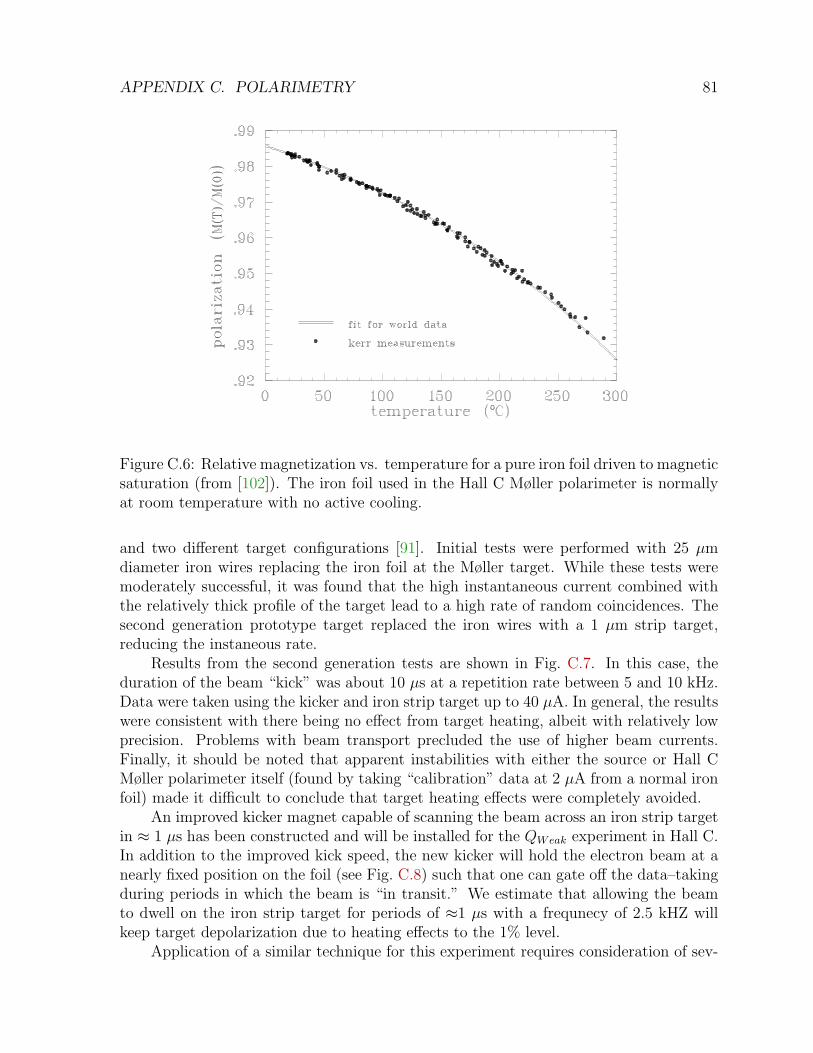
APPENDIX C. POLARIMETRY 81
Figure C.6: Relative magnetization vs. temperature for a pure iron foil driven to magneticsaturation (from [102]). The iron foil used in the Hall C Møller polarimeter is normallyat room temperature with no active cooling.
and two different target configurations [91]. Initial tests were performed with 25 µmdiameter iron wires replacing the iron foil at the Møller target. While these tests weremoderately successful, it was found that the high instantaneous current combined withthe relatively thick profile of the target lead to a high rate of random coincidences. Thesecond generation prototype target replaced the iron wires with a 1 µm strip target,reducing the instaneous rate.
Results from the second generation tests are shown in Fig. C.7. In this case, theduration of the beam “kick” was about 10 µs at a repetition rate between 5 and 10 kHz.Data were taken using the kicker and iron strip target up to 40 µA. In general, the resultswere consistent with there being no effect from target heating, albeit with relatively lowprecision. Problems with beam transport precluded the use of higher beam currents.Finally, it should be noted that apparent instabilities with either the source or Hall CMøller polarimeter itself (found by taking “calibration” data at 2 µA from a normal ironfoil) made it difficult to conclude that target heating effects were completely avoided.
An improved kicker magnet capable of scanning the beam across an iron strip targetin ≈ 1 µs has been constructed and will be installed for the QWeak experiment in Hall C.In addition to the improved kick speed, the new kicker will hold the electron beam at anearly fixed position on the foil (see Fig. C.8) such that one can gate off the data–takingduring periods in which the beam is “in transit.” We estimate that allowing the beamto dwell on the iron strip target for periods of ≈1 µs with a frequnecy of 2.5 kHZ willkeep target depolarization due to heating effects to the 1% level.
Application of a similar technique for this experiment requires consideration of sev-
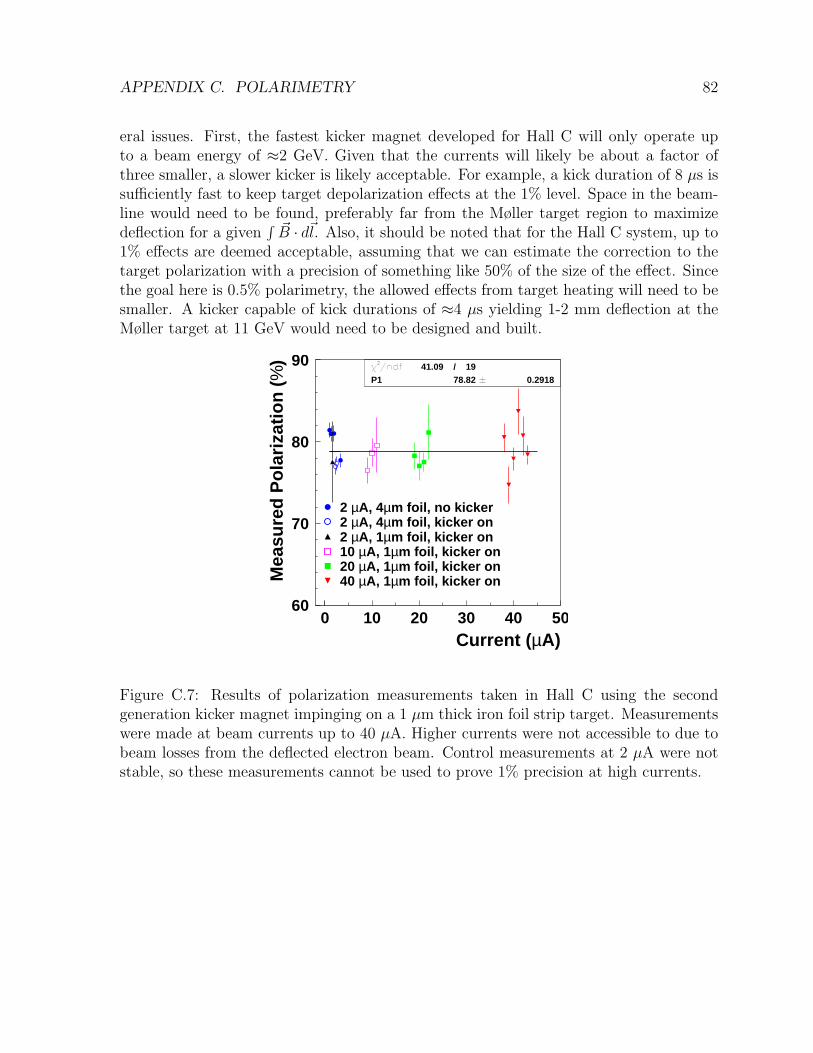
APPENDIX C. POLARIMETRY 82
eral issues. First, the fastest kicker magnet developed for Hall C will only operate upto a beam energy of ≈2 GeV. Given that the currents will likely be about a factor ofthree smaller, a slower kicker is likely acceptable. For example, a kick duration of 8 µs issufficiently fast to keep target depolarization effects at the 1% level. Space in the beam-line would need to be found, preferably far from the Møller target region to maximizedeflection for a given
∫ ~B · d~l. Also, it should be noted that for the Hall C system, up to1% effects are deemed acceptable, assuming that we can estimate the correction to thetarget polarization with a precision of something like 50% of the size of the effect. Sincethe goal here is 0.5% polarimetry, the allowed effects from target heating will need to besmaller. A kicker capable of kick durations of ≈4 µs yielding 1-2 mm deflection at theMøller target at 11 GeV would need to be designed and built.
60
70
80
90
0 10 20 30 40 50
41.09 / 19P1 78.82 0.2918
2 µA, 4µm foil, no kicker2 µA, 4µm foil, kicker on2 µA, 1µm foil, kicker on10 µA, 1µm foil, kicker on20 µA, 1µm foil, kicker on40 µA, 1µm foil, kicker on
Current (µA)
Mea
sure
d P
ola
riza
tio
n (
%)
Figure C.7: Results of polarization measurements taken in Hall C using the secondgeneration kicker magnet impinging on a 1 µm thick iron foil strip target. Measurementswere made at beam currents up to 40 µA. Higher currents were not accessible to due tobeam losses from the deflected electron beam. Control measurements at 2 µA were notstable, so these measurements cannot be used to prove 1% precision at high currents.
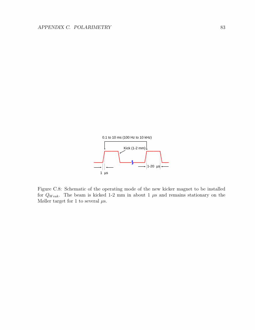
APPENDIX C. POLARIMETRY 83
1 µs
Kick (1-2 mm)
0.1 to 10 ms (100 Hz to 10 kHz)
1-20 µs
Figure C.8: Schematic of the operating mode of the new kicker magnet to be installedfor QWeak. The beam is kicked 1-2 mm in about 1 µs and remains stationary on theMøller target for 1 to several µs.
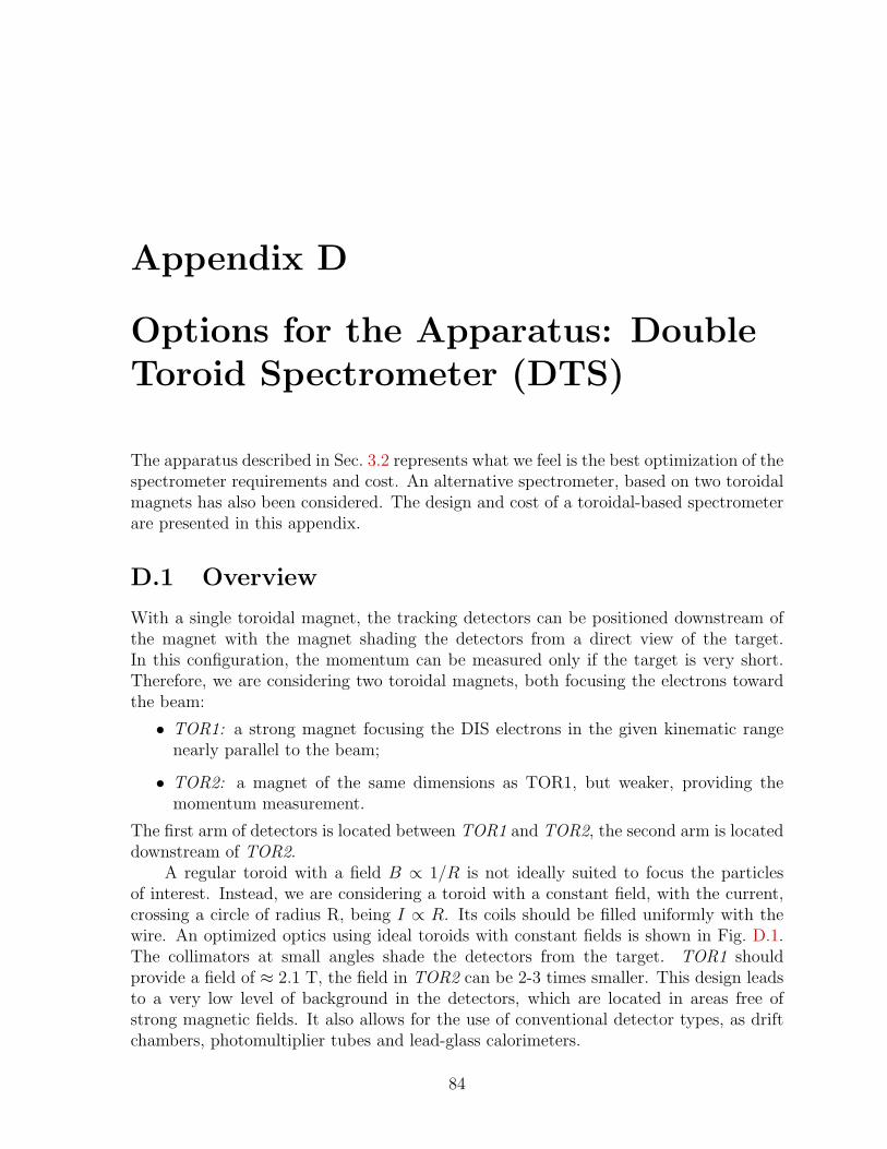
Appendix D
Options for the Apparatus: DoubleToroid Spectrometer (DTS)
The apparatus described in Sec. 3.2 represents what we feel is the best optimization of thespectrometer requirements and cost. An alternative spectrometer, based on two toroidalmagnets has also been considered. The design and cost of a toroidal-based spectrometerare presented in this appendix.
D.1 Overview
With a single toroidal magnet, the tracking detectors can be positioned downstream ofthe magnet with the magnet shading the detectors from a direct view of the target.In this configuration, the momentum can be measured only if the target is very short.Therefore, we are considering two toroidal magnets, both focusing the electrons towardthe beam:
• TOR1: a strong magnet focusing the DIS electrons in the given kinematic rangenearly parallel to the beam;
• TOR2: a magnet of the same dimensions as TOR1, but weaker, providing themomentum measurement.
The first arm of detectors is located between TOR1 and TOR2, the second arm is locateddownstream of TOR2.
A regular toroid with a field B ∝ 1/R is not ideally suited to focus the particlesof interest. Instead, we are considering a toroid with a constant field, with the current,crossing a circle of radius R, being I ∝ R. Its coils should be filled uniformly with thewire. An optimized optics using ideal toroids with constant fields is shown in Fig. D.1.The collimators at small angles shade the detectors from the target. TOR1 shouldprovide a field of ≈ 2.1 T, the field in TOR2 can be 2-3 times smaller. This design leadsto a very low level of background in the detectors, which are located in areas free ofstrong magnetic fields. It also allows for the use of conventional detector types, as driftchambers, photomultiplier tubes and lead-glass calorimeters.
84
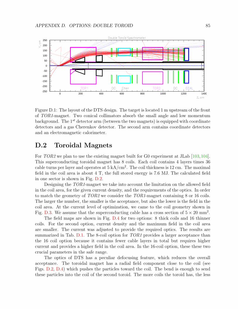
APPENDIX D. OPTIONS: DOUBLE TOROID 85
-250
-200
-150
-100
-50
0
50
100
150
200
250
0 200 400 600 800 1000 1200 1400
Figure D.1: The layout of the DTS design. The target is located 1 m upstream of the frontof TOR1-magnet. Two conical collimators absorb the small angle and low momentumbackground. The 1st detector arm (between the two magnets) is equipped with coordinatedetectors and a gas Cherenkov detector. The second arm contains coordinate detectorsand an electromagnetic calorimeter.
D.2 Toroidal Magnets
For TOR2 we plan to use the existing magnet built for G0 experiment at JLab [103,104].This superconducting toroidal magnet has 8 coils. Each coil contains 4 layers times 36cable turns per layer and operates at 5 kA/cm2. The coil thickness is 12 cm. The maximalfield in the coil area is about 4 T, the full stored energy is 7.6 MJ. The calculated fieldin one sector is shown in Fig. D.2.
Designing the TOR1-magnet we take into account the limitation on the allowed fieldin the coil area, for the given current density, and the requirements of the optics. In orderto match the geometry of TOR2 we consider the TOR1-magnet containing 8 or 16 coils.The larger the number, the smaller is the acceptance, but also the lower is the field in thecoil area. At the current level of optimization, we came to the coil geometry shown inFig. D.3. We assume that the superconducting cable has a cross section of 5× 20 mm2.
The field maps are shown in Fig. D.4 for two options: 8 thick coils and 16 thinnercoils. For the second option, current density and the maximum field in the coil areaare smaller. The current was adjusted to provide the required optics. The results aresummarized in Tab. D.1. The 8-coil option for TOR1 provides a larger acceptance thanthe 16 coil option because it contains fewer cable layers in total but requires highercurrent and provides a higher field in the coil area. In the 16-coil option, these these twocrucial parameters in the safe range.
The optics of DTS has a peculiar defocusing feature, which reduces the overallacceptance. The toroidal magnet has a radial field component close to the coil (seeFigs. D.2, D.4) which pushes the particles toward the coil. The bend is enough to sendthese particles into the coil of the second toroid. The more coils the toroid has, the less
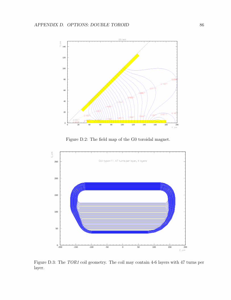
APPENDIX D. OPTIONS: DOUBLE TOROID 86
0
20
40
60
80
100
120
140
0 20 40 60 80 100 120 140 160 180 200
Figure D.2: The field map of the G0 toroidal magnet.
0
50
100
150
200
250
-200 -150 -100 -50 0 50 100 150 200
Figure D.3: The TOR1 coil geometry. The coil may contain 4-6 layers with 47 turns perlayer.

APPENDIX D. OPTIONS: DOUBLE TOROID 87
0
20
40
60
80
100
120
140
0 20 40 60 80 100 120 140 160 180 200
0
20
40
60
80
100
120
140
0 20 40 60 80 100 120 140 160 180 200
Figure D.4: The field maps of the TOR1 toroidal magnet. Top: 8 coils with 6 layers percoil, at 6.7 kA/cm2. Bottom: 16 coils with 4 layers per coil, at 5.0 kA/cm2
Magnet type coils layers/coil turns/layer kA/cm2 Bmax, T MJ
TOR2 G0 8 4 36 5.0 4.0 7.6TOR1 a) 8 6 47 6.7 6.0 60.0
b) 16 4 47 5.0 4.0 55.0
Table D.1: The parameters of the toroidal magnets considered.
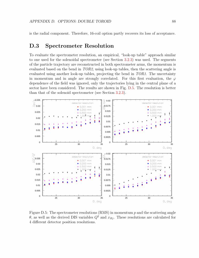
APPENDIX D. OPTIONS: DOUBLE TOROID 88
is the radial component. Therefore, 16-coil option partly recovers its loss of acceptance.
D.3 Spectrometer Resolution
To evaluate the spectrometer resolution, an empirical, “look-up table” approach similarto one used for the solenoidal spectrometer (see Section 3.2.3) was used. The segmentsof the particle trajectory are reconstructed in both spectrometer arms, the momentum isevaluated based on the bend in TOR2, using look-up tables, then the scattering angle isevaluated using another look-up tables, projecting the bend in TOR1. The uncertaintyin momentum and in angle are strongly correlated. For this first evaluation, the ϕdependence of the field was ignored, only the trajectories lying in the central plane of asector have been considered. The results are shown in Fig. D.5. The resolution is betterthan that of the solenoid spectrometer (see Section 3.2.3).
0
0.005
0.01
0.015
0.02
0.025
0.03
0.035
25 30 350
0.0025
0.005
0.0075
0.01
0.0125
0.015
0.0175
0.02
25 30 35
0
0.005
0.01
0.015
0.02
0.025
0.03
0.035
25 30 350
0.0025
0.005
0.0075
0.01
0.0125
0.015
0.0175
0.02
25 30 35
Figure D.5: The spectrometer resolutions (RMS) in momentum p and the scattering angleθ, as well as the derived DIS variables Q2 and xBj. These resolutions are calculated for4 different detector position resolutions.

APPENDIX D. OPTIONS: DOUBLE TOROID 89
Process DTS-8 DTS-16
DIS total 20 kHz 16.0 kHzDIS W > 2 GeV, xBj > 0.65 8 kHz 6.4 kHzπ− P > 0.3 GeV 200 kHz 160 kHz
Table D.2: Calculated DIS and pion rates for two TOR1 options: with 8 coils (DTS-8)and with 16 coils (DTS-16).
1
2
3
4
5
6
7
8
20 30 40
θ, deg
P, G
eV/c
Figure D.6: The DTS acceptance area in the p − θ plane (blue dots) matches well theDIS xBj > 0.65 sample (red dots).
D.4 The Acceptance and the Rates
The DIS and background rates were evaluated similar to the SoLID design (see Sec-tion 3.2.8). The rates calculated for various conditions are presented in Tab. D.2. TheDIS xBj > 0.65 rates are comparable to those for SoLID (see Table 3.3), but the pionrate is nearly 3 orders of magnitude lower. Also, the DIS 0.55 < xBj < 0.65 events aresuppressed and would require a separate run at lower magnetic fields. The acceptance ofDTS is extremely selective to a certain kinematics range, which is illustrated in Fig. D.6.
D.5 Implementation
In comparison with the SoLID design, the DTS design requires a new and complexmagnet to be built. The rest of the spectrometer, including the detectors is conceptually
APPENDIX D. OPTIONS: DOUBLE TOROID 90
much simpler than the SoLID spectrometer. Due to low backgrounds the requirementsto the detectors, PID and the trigger are relaxed in comparison with the SoLID design.However, because of the 2-arm setup, twice as many coordinate detectors are needed.
D.5.1 Magnets
Building TOR1 is a serious challenge because of the size, the coil complexity and thestored energy. The 16-coil magnet would operate in safe conditions as far as the super-conductor stability is concerned. The 8-coil version may be beyond the allowed area andfurther evaluation is necessary.
The G0 magnet will require a considerable refurbishing. The frontal wall has to beequipped with thin windows, similarly to the rear wall. The heavy shielding, installedinside the vacuum vessel, has to be removed.
D.5.2 Coordinate Detectors
Lower background rates in the toroid-based design will allow for the use of more con-ventional detectors. The minimal detector to accomplish the goals of the experimentneeds to have a threshold Cherenkov detector to π/e discrimination, tracking detectorsboth downstream an upstream of TOR2, trigger scintillators and a preshower/showercalorimeter system. In the following, these detectors will be described in greater detailand rough cost estimates are made for each element.
Tracking Chambers
The spectrometer will measure the bend of each particles trajectory in TOR2. To dothis accurately, two sets of tracking chambers are required on both the upstream anddownstream side of TOR2 for each of the 8 sectors, that is a total of 32 individualtracking chambers. The resolution of the spectrometer in terms of the relevant kinematicvariables as a function of the tracking resolution is shown in Fig. D.5. Each set oftracking chambers would consist of a u, u′ pair and a v, v′ pair. The chambers upstreamof TOR2 would cover radially from 100 to 150 cm, and the two chambers downstream ofTOR2 would cover from 50 to 150 cm radially. (See Fig. D.1.) The two options underconsideration for these chambers are an MWPC with 2 mm cells or a drift chamberwith 1 cm cells. Either chamber will give sufficient resolution for the measurements;although, the drift chamber or a finer pitched MWPC might be preferred as shown inFig. D.5. The MWPC has the advantage that it can handle 10× the rate as the driftchamber, based on geometry and the use of a gas with a faster drift velocity. It doesthis at the expense of more channels and the likely need for a recirculating gas system.The upstream (downstream) MWPC’s would require 250 (500) channels/plane. This iscompared with the 50 (100) channels for the drift chambers. In either case, the preampand readout could be done for approximately $33/channel using custom, FPGA-basedreadout cards similar to a design being implemented in Fermilab E-906/Drell-Yan. Basedon this and a very rough estimate of the cost of building 32 nearly-identical chambers the
APPENDIX D. OPTIONS: DOUBLE TOROID 91
entire tracking hardware and readout could be constructed for approximately $2.3M forthe drift chambers (without contingency or indirect costs) or approximately twice thatfor the MWPC solution because of the significant increase in readout channels.
Preshower and Shower Detectors
The preshower and shower detectors are needed for electron/pion separation. As a roughguide, we anticipate using a 10 cm thick (3.7 X0) Pb-Glass preshower followed by a 25 cmPb-Glass (9.3 X0) shower counter. This gives a total of 13 X0 of material. The PRIMEXcollaboration was able to obtain Pb-Glass for approximately $1/cm3 in a collaborationwith ITEP [105] in 1999, or around $1.30 today. While this collaboration has not beenexplored, we use this as a cost basis for Pb-Glass. Each of the eight sectors will haveapproximately 6,100 cm2 area so that the preshower counter will cost approximately $79kand the shower counter will cost approximately $198k. The sector can be covered by 16blocks of 10×10×(35−60) cm3 for the preshower and 66 blocks of 10×10×25 cm3 for theshower. These 82 channels/sector could be outfitted with photomultipliers/bases/shieldsfor approximately $300/channel with an additional $100/channel for readout electronics.The total cost for eight sectors would be approximately $2.5M (without contingency orindirect cots). It is likely that some amount of the Pb-Glass detectors could be recoveredfrom existing experiments which have been decommissioned.
Trigger Scintillators and Gas Cherenkov
In the DTS design there will be two sets of trigger scintillators, one before and one afterTOR2. These could be 10 cm wide strips aligned with the preshower counters. Basedon quotes from Eljen Technology, the scintillator and light guide material for each sectorshould cost around $4k, with the caveat that a substantial component of plastics is oil,the price of which has been fluctuating wildly in recent years. Using the same readoutcost/channel as for the shower counters ($400/channel) and 32 channels/sector, the totalcost per sector is $17k or $134k or the entire spectrometer.
The threshold Cherenkov would be set of eight volumes of relatively simple geometry.It is hoped that much of the technology being used in the Cherenkov for the CLAS12upgrade can be duplicated for the DTS Cherenkov counter, and might be realized foraround $400k. Unlike the preferred solenoid spectrometer solution, this Cherenkov willnot have large magnetic fields located near the photomultiplier tubes.
Summary of DTS Detectors and Cost
The particle position and identification detectors used in the DTS are envisioned asvery conventional nuclear physics detectors. These are proven technologies with relativeeasily justified cost estimates. Particle identification will be done with a combinationof a threshold Cherenkov counter for each sector and preshower/shower detectors. Themomentum measurement will be made by measuring the bend of the particle though theessentially dipole field in each toroid section with conventional drift chambers on each
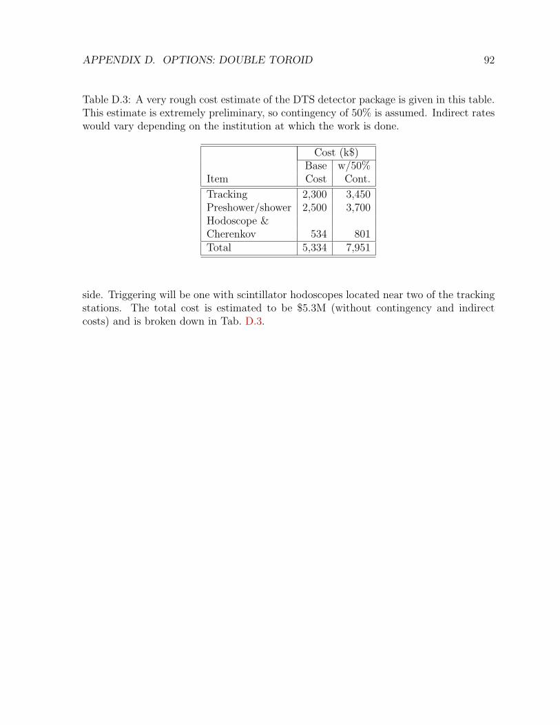
APPENDIX D. OPTIONS: DOUBLE TOROID 92
Table D.3: A very rough cost estimate of the DTS detector package is given in this table.This estimate is extremely preliminary, so contingency of 50% is assumed. Indirect rateswould vary depending on the institution at which the work is done.
Cost (k$)Base w/50%
Item Cost Cont.
Tracking 2,300 3,450Preshower/shower 2,500 3,700Hodoscope &Cherenkov 534 801Total 5,334 7,951
side. Triggering will be one with scintillator hodoscopes located near two of the trackingstations. The total cost is estimated to be $5.3M (without contingency and indirectcosts) and is broken down in Tab. D.3.
Bibliography
[1] T. Hobbs and W. Melnitchouk, “Finite-Q2 corrections to parity-violating DIS,”Phys. Rev., vol. D77, p. 114023, 2008, 0801.4791.
[2] A. Acha et al., “Precision Measurements of the Nucleon Strange Form Factors atQ2 ∼ 0.1-GeV2,” Phys. Rev. Lett., vol. 98, p. 032301, 2007, nucl-ex/0609002.
[3] K. A. Aniol et al., “Parity-violating electroweak asymmetry in e(pol.) p scattering,”Phys. Rev., vol. C69, p. 065501, 2004, nucl-ex/0402004.
[4] D. S. Armstrong et al., “Strange quark contributions to parity-violating asymme-tries in the forward G0 electron proton scattering experiment,” Phys. Rev. Lett.,vol. 95, p. 092001, 2005, nucl-ex/0506021.
[5] F. E. Maas et al., “Evidence for strange quark contributions to the nucleon’s formfactors at Q2 = 0.108-(GeV/c)2,” Phys. Rev. Lett., vol. 94, p. 152001, 2005, nucl-ex/0412030.
[6] C. J. Horowitz, S. J. Pollock, P. A. Souder, and R. Michaels, “Parity ViolatingMeasurements of Neutron Densities,” Phys. Rev., vol. C63, p. 025501, 2001, nucl-th/9912038.
[7] C. Y. Prescott et al., “Parity non-conservation in inelastic electron scattering,”Phys. Lett., vol. B77, pp. 347–352, 1978.
[8] C. Y. Prescott et al., “Further Measurements of Parity Nonconservation in Inelasticelectron Scattering,” Phys. Lett., vol. B84, p. 524, 1979.
[9] P. A. Souder et al., “Measurement of parity violation in the elastic scattering ofpolarized electrons from C-12,” Phys. Rev. Lett., vol. 65, pp. 694–697, 1990.
[10] P. L. Anthony et al., “Precision measurement of the weak mixing angle in Moellerscattering,” Phys. Rev. Lett., vol. 95, p. 081601, 2005, hep-ex/0504049.
[11] S.-L. Zhu, S. J. Puglia, B. R. Holstein, and M. J. Ramsey-Musolf, “The nu-cleon anapole moment and parity-violating e p scattering,” Phys. Rev., vol. D62,p. 033008, 2000, hep-ph/0002252.
93
BIBLIOGRAPHY 94
[12] R. D. Young, J. Roche, R. D. Carlini, and A. W. Thomas, “Extracting nucleonstrange and anapole form factors from world data,” Phys. Rev. Lett., vol. 97,p. 102002, 2006, nucl-ex/0604010.
[13] A. Accardi and W. Melnitchouk, “Target mass corrections for spin-dependent struc-ture functions in collinear factorization,” 2008, 0808.2397.
[14] X. C. Zheng, “Disparity e08-011.” URL http://hallaweb.jlab.org/
experiment/E05-007/.
[15] M. J. Ramsey-Musolf and S. Su, “Low energy precision test of supersymmetry,”Phys. Rept., vol. 456, pp. 1–88, 2008, hep-ph/0612057.
[16] A. Kurylov, M. J. Ramsey-Musolf, and S. Su, “Supersymmetric effects in parity-violating deep inelastic electron nucleus scattering,” Phys. Lett., vol. B582, pp. 222–228, 2004, hep-ph/0307270.
[17] J. T. Londergan and A. W. Thomas, “The validity of charge symmetry for partondistributions,” Prog. Part. Nucl. Phys., vol. 41, pp. 49–124, 1998, hep-ph/9806510.
[18] J. T. Londergan and A. W. Thomas, “Charge symmetry violation corrections todetermination of the Weinberg angle in neutrino reactions,” Phys. Rev., vol. D67,p. 111901, 2003, hep-ph/0303155.
[19] J. T. Londergan and A. W. Thomas, “Charge symmetry violating contributions toneutrino reactions,” Phys. Lett., vol. B558, pp. 132–140, 2003, hep-ph/0301147.
[20] G. P. Zeller et al., “A precise determination of electroweak parameters in neutrinonucleon scattering,” Phys. Rev. Lett., vol. 88, p. 091802, 2002, hep-ex/0110059.[Erratum-ibid. 90, 239902 (2003)].
[21] A. D. Martin, R. G. Roberts, W. J. Stirling, and R. S. Thorne, “Uncertaintiesof predictions from parton distributions. II: Theoretical errors,” Eur. Phys. J.,vol. C35, pp. 325–348, 2004, hep-ph/0308087.
[22] E. Sather, “Isospin violating quark distributions in the nucleon,” Phys. Lett.,vol. B274, pp. 433–438, 1992.
[23] E. N. Rodionov, A. W. Thomas, and J. T. Londergan, “Charge asymmetry ofparton distributions,” Mod. Phys. Lett., vol. A9, pp. 1799–1806, 1994.
[24] A. D. Martin, R. G. Roberts, W. J. Stirling, and R. S. Thorne, “Parton distributionsincorporating QED contributions,” Eur. Phys. J., vol. C39, pp. 155–161, 2005, hep-ph/0411040.
[25] M. Gluck, P. Jimenez-Delgado, and E. Reya, “Radiatively generated isospin viola-tions in the nucleon and the NuTeV anomaly,” Phys. Rev. Lett., vol. 95, p. 022002,2005, hep-ph/0503103.
BIBLIOGRAPHY 95
[26] J. T. Londergan, D. P. Murdock, and A. W. Thomas, “Parton charge symmetryviolation: Electromagnetic effects and W production asymmetries,” Phys. Rev.,vol. D73, p. 076004, 2006, hep-ph/0603208.
[27] J. T. Londergan, D. P. Murdock, and A. W. Thomas, “Experimental tests of chargesymmetry violation in parton distributions,” Phys. Rev., vol. D72, p. 036010, 2005,hep-ph/0507029.
[28] J. T. Londergan and A. W. Thomas, “Implications of current constraints on partoncharge symmetry,” J. Phys., vol. G31, pp. 1151–1163, 2005.
[29] M. Virchaux and A. Milsztajn, “A Measurement of alpha-s and higher twists froma QCD analysis of high statistics F-2 data on hydrogen and deuterium targets,”Phys. Lett., vol. B274, pp. 221–229, 1992.
[30] P. Amaudruz et al., “The ratio F2(n) / F2(p) in deep inelastic muon scattering,”Nucl. Phys., vol. B371, pp. 3–31, 1992.
[31] J. Blumlein and H. Bottcher, “Higher Twist Contributions to the Structure Func-tions Fp
2(x,Q2) and Fd2(x,Q2) at Large x and Higher Orders,” Phys. Lett., vol. B662,
pp. 336–340, 2008, 0802.0408.
[32] J. D. Bjorken, “Model independent remarks on electron - quark parity violatingneutral - current couplings,” Phys. Rev., vol. D18, p. 3239, 1978.
[33] L. Wolfenstein, “Testing the Weinberg-Salam model in polarized e d and e p deepinelastic scattering,” Nucl. Phys., vol. B146, p. 477, 1978.
[34] E. Derman, “Parity violation in polarized electron - deuteron scattering withoutthe parton model,” Phys. Rev., vol. D19, p. 133, 1979.
[35] S. J. Brodsky, “Dynamical higher-twist and high x phenomena: A window to quarkquark correlations in QCD,” 2000, hep-ph/0006310.
[36] P. Castorina and P. J. Mulders, “Twist four corrections to asymmetry in polarizedelectron Deuteron scattering,” Phys. Rev., vol. D31, pp. 2760–2764, 1985.
[37] S. Fajfer and R. J. Oakes, “Twist - Four Effects on the Asymmetry in PolarizedElectron Deuteron Scattering and Sin**2-Theta(W),” Phys. Rev., vol. D30, p. 1585,1984.
[38] R. L. Jaffe and M. Soldate, “Twist Four in the QCD Analysis of Leptoproduction,”Phys. Lett., vol. B105, pp. 467–472, 1981.
[39] S. Alekhin, S. Kulagin, and R. Petti, “Update of the global fit of PDFs includingthe low-Q DIS data,” 2008, 0810.4893.
BIBLIOGRAPHY 96
[40] U.-K. Yang, A. Bodek, and Q. Fan, “Parton distributions, d/u, and higher twistsat high x,” 1998, hep-ph/9806457.
[41] M. Tzanov et al., “Precise measurement of neutrino and anti-neutrino differentialcross sections,” Phys. Rev., vol. D74, p. 012008, 2006, hep-ex/0509010.
[42] W. Melnitchouk, I. R. Afnan, F. R. P. Bissey, and A. W. Thomas, “Comment on’Parton distributions, d/u, and higher twist effects at high x’,” Phys. Rev. Lett.,vol. 84, p. 5455, 2000, hep-ex/9912001.
[43] W. Melnitchouk and A. W. Thomas, “Neutron / proton structure function ratioat large x,” Phys. Lett., vol. B377, pp. 11–17, 1996, nucl-th/9602038.
[44] S. I. Alekhin, “Global fit to the charged leptons DIS data: α(s), parton distribu-tions, and high twists,” Phys. Rev., vol. D63, p. 094022, 2001, hep-ph/0011002.
[45] S. Kuhlmann et al., “Large-x parton distributions,” Phys. Lett., vol. B476, pp. 291–296, 2000, hep-ph/9912283.
[46] S. Bultmann, “The BoNuS experiment at Jefferson Lab,” AIP Conf. Proc., vol. 747,pp. 46–49, 2005.
[47] I. Cloet, W. Bentz, and A. W. Thomas. private communication.
[48] B. Aubert et al., “The BaBar detector,” Nucl. Instrum. Meth., vol. A479, pp. 1–116,2002, hep-ex/0105044.
[49] K. Halbach and R. F. Holsinger, “Superfish-a Computer Program for Evaluation ofRF Cavities with Cylindrical Symmetry,” Part. Accel., vol. 7, pp. 213–222, 1976.
[50] R. Brun et al., “GEANT Detector Description and Simulation Tool, CERN Pro-gram Library (1993),” We use GEANT version 3.21.
[51] “HEPDATA: Reaction Database.” URL http://www.slac.stanford.edu/
spires/hepdata/.
[52] D. E. Wiser, Inclusive photoproduction of protons, kaons, and pions at SLAC en-ergies. PhD thesis, U. of Wisconsin, 1977. UMI 77-19743.
[53] S. Bachmann et al., “Performance of GEM detectors in high intensity particlebeams,” Nucl. Instrum. Meth., vol. A470, pp. 548–561, 2001.
[54] B. Ketzer, Q. Weitzel, S. Paul, F. Sauli, and L. Ropelewski, “Performance of tripleGEM tracking detectors in the COMPASS experiment,” Nucl. Instrum. Meth.,vol. A535, pp. 314–318, 2004.
[55] J. Alcorn et al., “Basic Instrumentation for Hall A at Jefferson Lab,” Nucl. Instrum.Meth., vol. A522, pp. 294–346, 2004.

BIBLIOGRAPHY 97
[56] L. W. Mo and Y.-S. Tsai, “Radiative corrections to elastic and inelastic e p andmu p scattering,” Rev. Mod. Phys., vol. 41, pp. 205–235, 1969.
[57] W. J. Marciano and A. Sirlin, “On Some General Properties of the O(alpha) Cor-rections to Parity Violation in Atoms,” Phys. Rev., vol. D29, p. 75, 1984.
[58] K. Hagiwara et al., “Review of particle physics,” Phys. Rev., vol. D66, p. 010001,2002.
[59] S. Eidelman et al., “Review of particle physics,” Phys. Lett., vol. B592, p. 1, 2004.
[60] K. Abe et al., “A high-precision measurement of the left-right Z boson cross-sectionasymmetry,” Phys. Rev. Lett., vol. 84, pp. 5945–5949, 2000, hep-ex/0004026.
[61] K. Kumar, R. Michaels, P. Souder, and G. Urciuolli, “The lead radius experimentprex, e06002.” URL http://hallaweb.jlab.org/parity/prex/.
[62] K. Paschke and P. s. Souder, “Happex-iii, e05-009.”
[63] R. P. I. Carlini, “The qweak experiment.” URL http://www.jlab.org/Hall-C/
Qweak/index.html.
[64] P. Fabbricatore et al., “The Superconducting magnet for the BaBar detector ofthe PEP-II B factory at SLAC,” IEEE Trans. Magnetics, vol. 32, pp. 2210–2213,1996.
[65] R. A. Bell et al., “The BaBar superconducting coil: Design, construction and test,”Nucl. Phys. Proc. Suppl., vol. 78, pp. 559–564, 1999.
[66] D. Boutigny et al., “BaBar technical design report,” SLAC-R-0457.
[67] C. Bernet et al., “The 40-cm x 40-cm gaseous microstrip detector Micromegasfor the high-luminosity COMPASS experiment at CERN,” Nucl. Instrum. Meth.,vol. A536, pp. 61–69, 2005.
[68] E. Abat et al., “The ATLAS Transition Radiation Tracker (TRT) proportional drifttube: Design and performance,” JINST, vol. 3, p. P02013, 2008.
[69] M. Ziegler, P. Sievers, and U. Straumann, “A triple GEM detector with two-dimensional readout,” Nucl. Instrum. Meth., vol. A471, pp. 260–263, 2000.
[70] G. S. Atoian et al., “Development of shashlik calorimeter for KOPIO,” Nucl. In-strum. Meth., vol. A531, pp. 467–480, 2004, physics/0310047.
[71] G. S. Atoian et al., “An Improved Shashlyk Calorimeter,” Nucl. Instrum. Meth.,vol. A584, pp. 291–303, 2008, 0709.4514.
[72] A. Zoccoli, “The electromagnetic calorimeter of the HERA-B experiment,” Nucl.Instrum. Meth., vol. A446, pp. 246–252, 2000.
BIBLIOGRAPHY 98
[73] G. Avoni et al., “The electromagnetic calorimeter of the HERA-B experiment,”Nucl. Instrum. Meth., vol. A580, pp. 1209–1226, 2007.
[74] A. A. Alves et al., “The LHCb Detector at the LHC,” JINST, vol. 3, p. S08005,2008.
[75] Z. Fraenkel et al., “A hadron blind detector for the PHENIX experiment at RHIC,”Nucl. Instrum. Meth., vol. A546, pp. 466–480, 2005, physics/0502008.
[76] F. Sauli, “Novel Cherenkov photon detectors,” Nucl. Instrum. Meth., vol. A553,pp. 18–24, 2005.
[77] R. Chechik, A. Breskin, and C. Shalem, “Thick GEM-like multipliers: A sim-ple solution for large area UV-RICH detectors,” Nucl. Instrum. Meth., vol. A553,pp. 35–40, 2005, physics/0502131.
[78] N. Falletto et al., “Compton scattering off polarized electrons with a high finesseFabry-Perot cavity at JLab,” Nucl. Instrum. Meth., vol. A459, pp. 412–425, 2001.
[79] C. Møller, “Zur Theorie des Durchgangs schneller Elektronen durch Materie,” An-nalen der Physik, vol. 406, pp. 531–585, 1932.
[80] A. A. Kresnin and L. N. Rosentsveig, “Polarization asymmetry of møller scatter-ing,” Soviet JETP, vol. 5, pp. 288–292, 1957.
[81] A. M. Bincer, “Scattering of longitudinally polarized fermions,” Phys. Rev.,vol. 107, pp. 1434–1438, Sep 1957.
[82] P. S. Cooper et al., “Polarized electron Electron Scattering at GeV Energies,” Phys.Rev. Lett., vol. 34, p. 1589, 1975.
[83] B. Wagner et al., “A Møller polarimeter for CW and pulsed intermediate-energyelectron beams,” Nucl. Instrum. Meth., vol. A294, pp. 541–548, 1990.
[84] J. Arrington et al., “A Variable energy Møller polarimeter at the MIT Bates LinearAccelerator Center,” Nucl. Instrum. Meth., vol. A311, pp. 39–48, 1992.
[85] K. B. Beard et al., “Measurement of the polarization of a pulsed electron beam witha Møller polarimeter in the coincidence mode,” Nucl. Instrum. Meth., vol. A361,pp. 46–52, 1995.
[86] H. R. Band, G. Mitchell, R. Prepost, and T. Wright, “A Møller polarimeter forhigh energy electron beams,” Nucl. Instrum. Meth., vol. A400, pp. 24–33, 1997.
[87] A. V. Glamazdin et al., “Electron beam Moeller polarimeter at JLAB Hall A,”Fizika, vol. B8, pp. 91–95, 1999, hep-ex/9912063.
[88] M. Hauger et al., “A high-precision polarimeter,” Nucl. Instrum. Meth., vol. A462,pp. 382–392, 2001, nucl-ex/9910013.
BIBLIOGRAPHY 99
[89] P. Steiner, A. Feltham, I. Sick, M. Zeier, and B. Zihlmann, “A high-rate coincidenceMøller polarimeter,” Nucl. Instrum. Meth., vol. A419, pp. 105–120, 1998.
[90] G. G. Scott, “Review of gyromagnetic ratio experiments,” Rev. Mod. Phys., vol. 34,pp. 102–109, Jan 1962.
[91] D. Gaskell, D. G. Meekins, and C. Yan, “New methods for precision Møller po-larimetry,” Eur. Phys. J., vol. A32, pp. 561–564, 2007.
[92] L. G. Levchuk, “The Intraatomic motion of bound electrons as a possible sourceof a systematic error in electron beam polarization measurements by means of aMøller polarimeter,” Nucl. Instrum. Meth., vol. A345, pp. 496–499, 1994.
[93] E. Chudakov and V. Luppov, “Møller polarimetry with atomic hydrogen targets,”IEEE Trans. Nucl. Sci., vol. 51, pp. 1533–1540, 2004.
[94] E. Chudakov and V. Luppov, “Moeller polarimetry with atomic hydrogen targets,”Eur. Phys. J., vol. A24S2, pp. 123–126, 2005.
[95] E. Chudakov and V. Luppov, “Møller polarimetry with atomic hydrogen targets,”tech. rep., JLab, 2005. URL http://www.jlab.org/∼gen/hyd/loi 3.pdf.
[96] I. F. Silvera, “Ultimate fate of a gas of atomic hydrogen in a liquid-helium chamber:Recombination and burial,” Phys. Rev. B, vol. 29, pp. 3899–3904, Apr 1984.
[97] I. F. Silvera and J. T. M. Walraven, “Stabilization of atomic hydrogen at lowtemperature,” Phys. Rev. Lett., vol. 44, pp. 164–168, Jan 1980.
[98] I. F. Silvera and J. T. M. Walraven, “Spin polarized atomic hydrogen,” Progressin Low Temperature Physics, vol. X, pp. 139–370, 1986.
[99] T. Roser et al., “Microwave driven extraction of stabilized spin polarized atomichydrogen,” Nucl. Instrum. Meth., vol. A301, pp. 42–46, 1991.
[100] M. Mertig, V. G. Luppov, T. Roser, and B. Vuaridel, “Continuous density mea-surement of atomic hydrogen by means of a bolometer,” Rev. Sci. Instrum., vol. 62,pp. 251–252, 1991.
[101] M. D. Miller and L. H. Nosanow, “Possible ”new” quantum systems. ii. propertiesof the isotopes of spin-aligned hydrogen,” Phys. Rev. B, vol. 15, pp. 4376–4385,May 1977.
[102] L. V. de Bever, J. Jourdan, M. Loppacher, S. Robinson, I. Sick, and J. Zhao, “Atarget for precise mller polarimetry,” Nucl. Instrum. Meth., vol. A400, no. 2-3,pp. 379 – 386, 1997.
[103] P. D. Brindza, D. Beck, R. Laszewski, L. Bartoszek, R. Wands, and D. Mitchell,“Superconducting toroidal magnet design for the G0 experiment at TJNAF,” IEEETrans. Appl. Supercond. (USA), vol. 7, no. 2, pp. 618–621, 1997.

BIBLIOGRAPHY 100
[104] P. D. Brindza, D. Beck, K. Nakahara, D. Spayde, S. Williamson, T. A. Antaya,M. Trepanitis, and T. Brandsberg, “The G0 spectrometer superconducting magnetsystem: from a challenging construction to reliable operations,” IEEE Trans. Appl.Supercond. (USA), vol. 16, no. 2, pp. 248–252, 2006.
[105] A. Gasparian et al., “Conceptual Design Report: A Precision Measurement of theNeutral Pion Lifetime via the Primakoff Effect,” 1999.