Embed Size (px)
Citation preview

American Institute of Aeronautics and Astronautics
1
Practical Aspects of Real-Time Modeling
for the Learn-to-Fly Concept
Eugene A. Morelli1
NASA Langley Research Center, Hampton, Virginia, 23681
Practical aspects of autonomous onboard real-time modeling for the NASA Learn-to-Fly
concept are examined using flight data from two subscale test aircraft. A practical real-time
global nonlinear aerodynamic modeling method is developed and explained, along with the
multiple-input excitation needed for effective real-time modeling. Critical issues for
integrating real-time global nonlinear aerodynamic modeling and local linear modeling with
the real-time learning adaptive control and guidance elements of the Learn-to-Fly algorithm
are identified and discussed. Real-time modeling results from NASA Learn-to-Fly flight
demonstrations are presented and evaluated using model fit metrics and prediction tests.
Nomenclature
x y za ,a ,a = body-axis translational accelerometer measurements, g
b = wing span, ft
c = wing mean aerodynamic chord, ft
X Y ZC ,C ,C = body-axis nondimensional aerodynamic force coefficients
l m nC ,C ,C = body-axis nondimensional aerodynamic moment coefficients
x y z xzI , I , I , I = inertia tensor elements, slug-ft2
m = mass, slug
max = maximum
min = minimum
N = number of data points
p, q, r = body-axis roll, pitch, and yaw rates, rad/s or deg/s
q = dynamic pressure, lbf/ft2
rms = root mean square
S = wing reference area, ft2
V = true airspeed, ft/s
= angle of attack, rad or deg
= sideslip angle, rad or deg
a e r f, , , = aileron, elevator, rudder, and flap deflections, rad or deg
, , = Euler roll, pitch, and yaw angles, rad or deg
p = propeller rotational speed, rev/min
Subscripts
cg = center of gravity
l = left
i = inboard
1 Research Engineer, Dynamic Systems and Control Branch, MS 308, AIAA Associate Fellow
American Institute of Aeronautics and Astronautics
2
o = outboard
r = right
ref = reference
Superscripts
T = transpose
= estimate
= time derivative
–1 = matrix inverse
= mean
Acronyms
CFD = Computational Fluid Dynamics
INS = Inertial Navigation System
NASA = National Aeronautics and Space Administration
PTI = Programmed Test Inputs
SIDPAC = System IDentification Programs for AirCraft
I. Introduction
HE goal of the NASA Learn-to-Fly initiative is to develop a global aircraft model and full-envelope flight
control and guidance autonomously onboard the aircraft in real time, without ground testing or human analyst
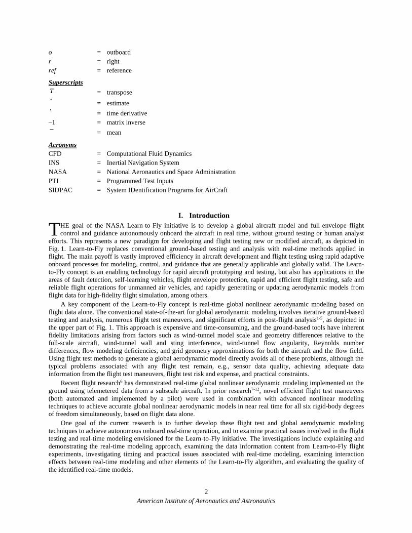
efforts. This represents a new paradigm for developing and flight testing new or modified aircraft, as depicted in
Fig. 1. Learn-to-Fly replaces conventional ground-based testing and analysis with real-time methods applied in
flight. The main payoff is vastly improved efficiency in aircraft development and flight testing using rapid adaptive
onboard processes for modeling, control, and guidance that are generally applicable and globally valid. The Learn-
to-Fly concept is an enabling technology for rapid aircraft prototyping and testing, but also has applications in the
areas of fault detection, self-learning vehicles, flight envelope protection, rapid and efficient flight testing, safe and
reliable flight operations for unmanned air vehicles, and rapidly generating or updating aerodynamic models from
flight data for high-fidelity flight simulation, among others.
A key component of the Learn-to-Fly concept is real-time global nonlinear aerodynamic modeling based on
flight data alone. The conventional state-of-the-art for global aerodynamic modeling involves iterative ground-based
testing and analysis, numerous flight test maneuvers, and significant efforts in post-flight analysis1-5, as depicted in
the upper part of Fig. 1. This approach is expensive and time-consuming, and the ground-based tools have inherent
fidelity limitations arising from factors such as wind-tunnel model scale and geometry differences relative to the
full-scale aircraft, wind-tunnel wall and sting interference, wind-tunnel flow angularity, Reynolds number
differences, flow modeling deficiencies, and grid geometry approximations for both the aircraft and the flow field.
Using flight test methods to generate a global aerodynamic model directly avoids all of these problems, although the
typical problems associated with any flight test remain, e.g., sensor data quality, achieving adequate data
information from the flight test maneuvers, flight test risk and expense, and practical constraints.
Recent flight research6 has demonstrated real-time global nonlinear aerodynamic modeling implemented on the
ground using telemetered data from a subscale aircraft. In prior research7-12, novel efficient flight test maneuvers
(both automated and implemented by a pilot) were used in combination with advanced nonlinear modeling
techniques to achieve accurate global nonlinear aerodynamic models in near real time for all six rigid-body degrees
of freedom simultaneously, based on flight data alone.
One goal of the current research is to further develop these flight test and global aerodynamic modeling
techniques to achieve autonomous onboard real-time operation, and to examine practical issues involved in the flight
testing and real-time modeling envisioned for the Learn-to-Fly initiative. The investigations include explaining and
demonstrating the real-time modeling approach, examining the data information content from Learn-to-Fly flight
experiments, investigating timing and practical issues associated with real-time modeling, examining interaction
effects between real-time modeling and other elements of the Learn-to-Fly algorithm, and evaluating the quality of
the identified real-time models.
T
American Institute of Aeronautics and Astronautics
3
Learn-To-Fly Concept
Dr. Gene Morelli, NASA LaRC 2
Ground-based
aerodynamics:
• CFD
• Wind Tunnel
Simulation
Model
Control Law
Design
Flight Test
Learning Control
Real-Time Modeling
Learn-to-Fly seeks to replace the current process …
…with a new paradigm
Real-Time Guidance
Figure 1. Comparison of conventional aircraft development with the Learn-to-Fly concept
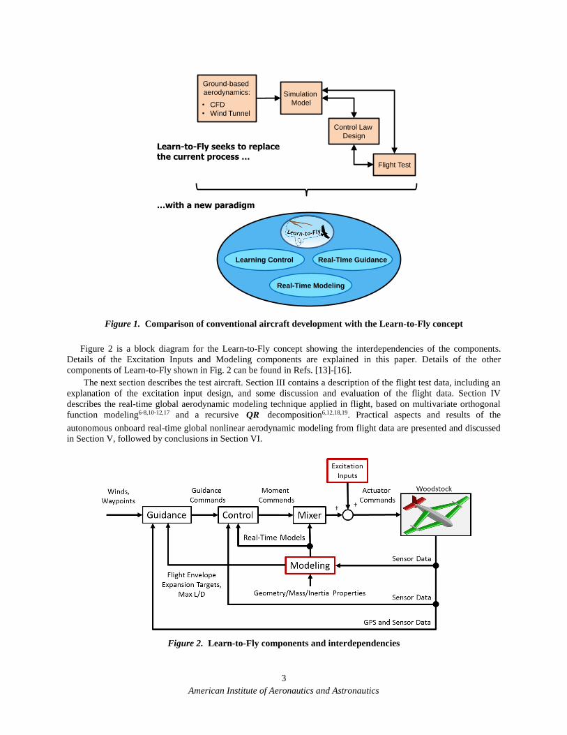
Figure 2 is a block diagram for the Learn-to-Fly concept showing the interdependencies of the components.
Details of the Excitation Inputs and Modeling components are explained in this paper. Details of the other
components of Learn-to-Fly shown in Fig. 2 can be found in Refs. [13]-[16].
The next section describes the test aircraft. Section III contains a description of the flight test data, including an
explanation of the excitation input design, and some discussion and evaluation of the flight data. Section IV
describes the real-time global aerodynamic modeling technique applied in flight, based on multivariate orthogonal
function modeling6-8,10-12,17 and a recursive QR decomposition6,12,18,19. Practical aspects and results of the
autonomous onboard real-time global nonlinear aerodynamic modeling from flight data are presented and discussed
in Section V, followed by conclusions in Section VI.
Figure 2. Learn-to-Fly components and interdependencies
American Institute of Aeronautics and Astronautics
4
The real-time modeling software developed and applied in this work was written in MATLAB®, implemented in
Simulink® using MATLAB® function blocks, integrated with the other components of the Learn-to-Fly algorithm
implemented in Simulink®, then autocoded onto the flight computer. Some of the real-time modeling software came
from the software toolbox called System IDentification Programs for AirCraft, or SIDPAC12,20.
II. Aircraft
Two subscale aircraft, named Woodstock and E1, were used for Learn-to-Fly flight testing. Woodstock is an
intentionally complex and unusual custom-designed glider, and E1 is a commercial off-the-shelf conventional low-
wing propeller aircraft.
A. Woodstock
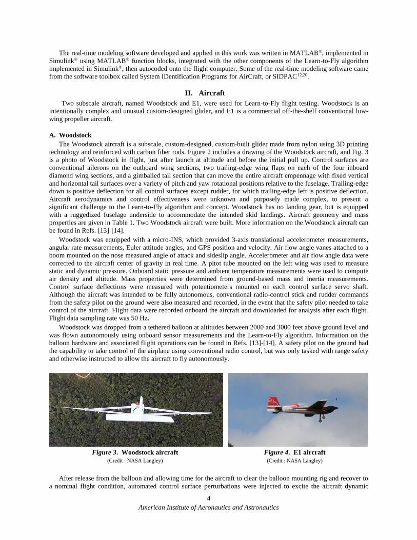
The Woodstock aircraft is a subscale, custom-designed, custom-built glider made from nylon using 3D printing
technology and reinforced with carbon fiber rods. Figure 2 includes a drawing of the Woodstock aircraft, and Fig. 3
is a photo of Woodstock in flight, just after launch at altitude and before the initial pull up. Control surfaces are
conventional ailerons on the outboard wing sections, two trailing-edge wing flaps on each of the four inboard
diamond wing sections, and a gimballed tail section that can move the entire aircraft empennage with fixed vertical
and horizontal tail surfaces over a variety of pitch and yaw rotational positions relative to the fuselage. Trailing-edge
down is positive deflection for all control surfaces except rudder, for which trailing-edge left is positive deflection.
Aircraft aerodynamics and control effectiveness were unknown and purposely made complex, to present a
significant challenge to the Learn-to-Fly algorithm and concept. Woodstock has no landing gear, but is equipped
with a ruggedized fuselage underside to accommodate the intended skid landings. Aircraft geometry and mass
properties are given in Table 1. Two Woodstock aircraft were built. More information on the Woodstock aircraft can
be found in Refs. [13]-[14].
Woodstock was equipped with a micro-INS, which provided 3-axis translational accelerometer measurements,
angular rate measurements, Euler attitude angles, and GPS position and velocity. Air flow angle vanes attached to a
boom mounted on the nose measured angle of attack and sideslip angle. Accelerometer and air flow angle data were
corrected to the aircraft center of gravity in real time. A pitot tube mounted on the left wing was used to measure
static and dynamic pressure. Onboard static pressure and ambient temperature measurements were used to compute
air density and altitude. Mass properties were determined from ground-based mass and inertia measurements.
Control surface deflections were measured with potentiometers mounted on each control surface servo shaft.
Although the aircraft was intended to be fully autonomous, conventional radio-control stick and rudder commands
from the safety pilot on the ground were also measured and recorded, in the event that the safety pilot needed to take
control of the aircraft. Flight data were recorded onboard the aircraft and downloaded for analysis after each flight.
Flight data sampling rate was 50 Hz.
Woodstock was dropped from a tethered balloon at altitudes between 2000 and 3000 feet above ground level and
was flown autonomously using onboard sensor measurements and the Learn-to-Fly algorithm. Information on the
balloon hardware and associated flight operations can be found in Refs. [13]-[14]. A safety pilot on the ground had
the capability to take control of the airplane using conventional radio control, but was only tasked with range safety
and otherwise instructed to allow the aircraft to fly autonomously.
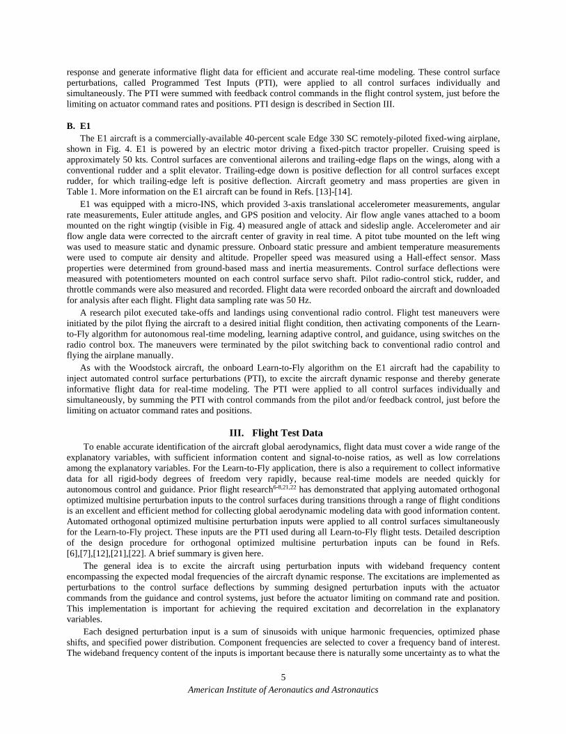
Figure 3. Woodstock aircraft Figure 4. E1 aircraft
(Credit : NASA Langley) (Credit : NASA Langley)
After release from the balloon and allowing time for the aircraft to clear the balloon mounting rig and recover to
a nominal flight condition, automated control surface perturbations were injected to excite the aircraft dynamic
American Institute of Aeronautics and Astronautics
5
response and generate informative flight data for efficient and accurate real-time modeling. These control surface
perturbations, called Programmed Test Inputs (PTI), were applied to all control surfaces individually and
simultaneously. The PTI were summed with feedback control commands in the flight control system, just before the
limiting on actuator command rates and positions. PTI design is described in Section III.
B. E1
The E1 aircraft is a commercially-available 40-percent scale Edge 330 SC remotely-piloted fixed-wing airplane,
shown in Fig. 4. E1 is powered by an electric motor driving a fixed-pitch tractor propeller. Cruising speed is
approximately 50 kts. Control surfaces are conventional ailerons and trailing-edge flaps on the wings, along with a
conventional rudder and a split elevator. Trailing-edge down is positive deflection for all control surfaces except
rudder, for which trailing-edge left is positive deflection. Aircraft geometry and mass properties are given in
Table 1. More information on the E1 aircraft can be found in Refs. [13]-[14].
E1 was equipped with a micro-INS, which provided 3-axis translational accelerometer measurements, angular
rate measurements, Euler attitude angles, and GPS position and velocity. Air flow angle vanes attached to a boom
mounted on the right wingtip (visible in Fig. 4) measured angle of attack and sideslip angle. Accelerometer and air
flow angle data were corrected to the aircraft center of gravity in real time. A pitot tube mounted on the left wing
was used to measure static and dynamic pressure. Onboard static pressure and ambient temperature measurements
were used to compute air density and altitude. Propeller speed was measured using a Hall-effect sensor. Mass
properties were determined from ground-based mass and inertia measurements. Control surface deflections were
measured with potentiometers mounted on each control surface servo shaft. Pilot radio-control stick, rudder, and
throttle commands were also measured and recorded. Flight data were recorded onboard the aircraft and downloaded
for analysis after each flight. Flight data sampling rate was 50 Hz.
A research pilot executed take-offs and landings using conventional radio control. Flight test maneuvers were
initiated by the pilot flying the aircraft to a desired initial flight condition, then activating components of the Learn-
to-Fly algorithm for autonomous real-time modeling, learning adaptive control, and guidance, using switches on the
radio control box. The maneuvers were terminated by the pilot switching back to conventional radio control and
flying the airplane manually.
As with the Woodstock aircraft, the onboard Learn-to-Fly algorithm on the E1 aircraft had the capability to
inject automated control surface perturbations (PTI), to excite the aircraft dynamic response and thereby generate
informative flight data for real-time modeling. The PTI were applied to all control surfaces individually and
simultaneously, by summing the PTI with control commands from the pilot and/or feedback control, just before the
limiting on actuator command rates and positions.
III. Flight Test Data
To enable accurate identification of the aircraft global aerodynamics, flight data must cover a wide range of the
explanatory variables, with sufficient information content and signal-to-noise ratios, as well as low correlations
among the explanatory variables. For the Learn-to-Fly application, there is also a requirement to collect informative
data for all rigid-body degrees of freedom very rapidly, because real-time models are needed quickly for
autonomous control and guidance. Prior flight research6-8,21,22 has demonstrated that applying automated orthogonal
optimized multisine perturbation inputs to the control surfaces during transitions through a range of flight conditions
is an excellent and efficient method for collecting global aerodynamic modeling data with good information content.
Automated orthogonal optimized multisine perturbation inputs were applied to all control surfaces simultaneously
for the Learn-to-Fly project. These inputs are the PTI used during all Learn-to-Fly flight tests. Detailed description
of the design procedure for orthogonal optimized multisine perturbation inputs can be found in Refs.
[6],[7],[12],[21],[22]. A brief summary is given here.
The general idea is to excite the aircraft using perturbation inputs with wideband frequency content
encompassing the expected modal frequencies of the aircraft dynamic response. The excitations are implemented as
perturbations to the control surface deflections by summing designed perturbation inputs with the actuator
commands from the guidance and control systems, just before the actuator limiting on command rate and position.
This implementation is important for achieving the required excitation and decorrelation in the explanatory
variables.
Each designed perturbation input is a sum of sinusoids with unique harmonic frequencies, optimized phase
shifts, and specified power distribution. Component frequencies are selected to cover a frequency band of interest.
The wideband frequency content of the inputs is important because there is naturally some uncertainty as to what the

American Institute of Aeronautics and Astronautics
6
modal frequencies are for the aircraft in flight, and the wideband inputs provide robustness to that uncertainty. Phase
shifts for the sinusoidal components of each input are optimized to achieve low peak-to-peak amplitude for the sum
of sinusoids. Amplitudes of the individual sinusoidal components can be selected to achieve a specific power
distribution.
Multiple inputs are designed to be mutually orthogonal in both the time domain and the frequency domain, and
are designed for high data information content in all axes over a short time period, while minimizing excursions
from the nominal flight condition. The mutual orthogonality of the inputs allows simultaneous application of
multiple inputs, which reduces the required excitation time, but even more importantly for this work, provides
continuous multi-axis excitation as the aircraft flies through various flight conditions.
Each perturbation input ju , which is to be applied to the jth individual control surface, is a sum of harmonic
sinusoids with individual phase shifts k ,
1 2
2j k k
k , , ,M
kA sin
T
tu 1 2 ij , , ,n (1)
where M is the total number of available harmonically-related frequencies, T is the time length of the excitation, kA
is the amplitude for the kth sinusoidal component, and t is the time vector. Each of the in inputs is the sum of
selected components from the pool of M harmonic sinusoids with frequencies 2 1 2k k T , k , , ,M , where
2M M T represents the upper limit of the frequency band for the excitation inputs. The interval 1 M,
rad/s specifies the range of frequencies where the aircraft dynamics are expected to lie.
The mutual orthogonality of the PTI in the time domain comes from the fact that all sinusoidal components of
each input are harmonic sinusoids with the same base period T, but unique harmonic frequencies. Orthogonality in
the frequency domain comes from using unique frequencies for the component sinusoids included in each input.
If the phase angles k in Eq. (1) were chosen at random on the interval , rad, then in general, the
various harmonic components would add together at some points to produce an input ju with relatively large
amplitude excursions. This is undesirable, because it can result in the dynamic system being moved too far from the
reference condition for the test. To prevent this, the phase angles k for each of the selected harmonic components
are optimized to minimize the relative peak factor RPF , defined by
2
2 22
j j j j
jT
jj j
max min max minRPF
rmsN
u u u uu
uu u
1 2 ij , , ,n (2)
Relative peak factor is a measure of the efficiency of an input for dynamic modeling purposes, in terms of the
amplitude of the input divided by a measure of the input energy. Low values of relative peak factors are desirable for
highly efficient and effective aerodynamic modeling, because the objective is to excite the dynamic system with
good input energy over a variety of frequencies while minimizing the input amplitudes in the time domain, to avoid
driving the dynamic system too far away from the reference condition. For each input with more than one sinusoidal
component, as in Eq. (1), minimum RPF is achieved by adjusting the phase angles k for each individual sinusoidal
component of the input. The resulting optimization problem is non-convex; however, a simplex algorithm can be
applied to find a solution12,21-23.
The integers k specifying the harmonic frequencies for the jth input ju are selected to be unique to that input,
but are not necessarily consecutive. A good approach for multiple inputs is to assign integers k to each input
alternately. This is illustrated in Fig. 5 for flight test maneuver design on the E1 aircraft. There are 6 inputs in this
case: elevator, rudder, and ailerons and flaps on the left and right wings. The harmonic frequencies were interleaved
among these six inputs to achieve wideband frequency content in each input, for robustness in the excitation and to
enable accurate individual control surface effectiveness estimates. Because each input has wideband frequency
content, the same input design can be applied at various flight conditions, which simplifies the excitation strategy

American Institute of Aeronautics and Astronautics
7
and reduces flight computer memory requirements. Figure 6 shows time series for the PTI designed using the
frequency content depicted in Fig. 5.
To achieve a uniform power distribution, the kA are selected as
k
AA k
n (3)
where n is the number of sinusoidal components included in the summation of Eq. (1), and A is the amplitude of
the composite input ju . Therefore, with uniform power distribution, selection of the kA reduces to selecting a
single value for the input amplitude A . Each input ju can of course have arbitrary amplitude A , subject to
practical flight test and modeling constraints. The different heights of the bars in Fig. 5 reflect the different
amplitudes used for the PTI applied to each individual control surface.
Figure 6. E1 multiple orthogonal optimized multisine inputs
Figure 5. E1 multiple orthogonal optimized multisine input power spectra
deg
lf
deg
rf
deg
ra
deg
la
deg
e
deg
r
rf
lf
la
ra
e
r

American Institute of Aeronautics and Astronautics
8
The PTI design shown in Figs. 5 and 6 was used throughout the E1 flight testing, with only input amplitude
adjustments made after the first flight, to achieve acceptable signal-to-noise ratios for the measured aircraft
responses. This adjustment was necessary because there was no prior information for either the measurement noise
levels or the control surface effectiveness. Because the PTI are sums of harmonic sinusoids with a common base
period T, they are periodic for the excitation period T, so that the PTI can be applied repeatedly without any
discontinuities in magnitude or slope.
The PTI described here were used to provide multi-axis flight data with high information content and low
correlations among the explanatory variables over a large range of flight conditions, as required for accurate and
efficient global aerodynamic modeling. The multiple-input design with orthogonality was important for Learn-to-Fly
because the aircraft dynamics could be excited rapidly and effectively in all axes simultaneously, so that informative
data could be collected quickly to enable accurate real-modeling as soon as possible. The same approach was used
for both Woodstock and E1, with the difference in the PTI design mainly the number of control surfaces: 12 for
Woodstock, and 6 for E1.
Table 2 provides elevator PTI design information for E1 Learn-to-Fly flight tests. PTI design information for
the other control surfaces was analogous. Table 3 contains descriptions of the research flight tests for E1, and
Table 4 contains analogous information for Woodstock.
Figure 7 shows cross plots of selected explanatory variable data from E1 flight 3. These plots demonstrate that a
wide range of the explanatory variables was swept through during the Learn-to-Fly flight tests with PTI active. Note
that the cross plots generally do not resemble straight lines, which means that the explanatory variable data had low
pairwise correlations. Low correlations mean that the dependencies of the aircraft aerodynamics on the explanatory
variables can be identified accurately and without ambiguity. Cross plots for other aircraft states and controls used
for global aerodynamic modeling were similar to Fig. 7 in that the plots indicated low correlations and wide ranges
of coverage for the explanatory variables.
Because the PTI were composed of sinusoids with various frequencies and phase angles, and were optimized
for small total amplitude, applying these inputs simultaneously to the aircraft produces a dynamic response similar
to what might be seen in flight through light to moderate turbulence. Consequently, the aircraft stays near the
reference condition, but exhibits rich dynamic response about that condition. In practice, guidance and feedback
control act to spoil the perfect orthogonality (zero pairwise correlations) of the designed PTI. However, good
modeling results require only low correlations, not zero correlations, so that the slightly correlated inputs that result
from applying orthogonal PTI with guidance and feedback control acting still work very well.
Figure 7. E1 flight data cross plots

American Institute of Aeronautics and Astronautics
9
IV. Real-Time Global Aerodynamic Modeling
The modeling objective for Learn-to-Fly is to identify a global nonlinear model in real time for each
nondimensional aerodynamic force and moment coefficient as a function of explanatory variables that can be
measured, such as angle of attack, sideslip angle, body-axis angular rates, and control surface deflections. There are
two main difficulties in doing this: 1) designing an experiment to collect informative dynamic data rapidly, which
was addressed in Section III, and 2) identifying an accurate global nonlinear model in real time, which is the subject
of this section.
Global aerodynamic modeling involves identifying complex connections between the explanatory variables
(such as angle of attack and control surface deflections) and the quantities to be predicted (such as nondimensional
pitching moment coefficient), often called the dependent variables. An effective approach to identifying such
connections from the data is to evaluate candidate functions of the explanatory variables for effectiveness in
accurately characterizing the dependent variable, using data transformations and statistical criteria.
In previous work6, a method for real-time global aerodynamic modeling was developed and demonstrated, with
all calculations done on the ground using telemetered flight data. This method used recursive orthogonalization to
isolate and quantify the modeling capability of individual candidate linear and nonlinear model terms, then applied
statistical metrics computed from the data to select which of the orthogonalized model terms should be included in
the model6-8,10-12,17. After this model structure determination step, model parameter values and uncertainties were
calculated. The real-time modeling in Learn-to-Fly employs this general approach, with all computations done in
real time by the onboard flight computer, to identify global nonlinear aerodynamic models valid over large ranges of
the explanatory variables.
The next subsections describe the general nonlinear aerodynamic modeling problem using nondimensional
aerodynamic coefficients, recursive real-time orthogonalization of the candidate model terms, modeling metrics, and
the method used for real-time global aerodynamic modeling.
A. Nondimensional Aerodynamic Coefficient Modeling
For global aerodynamic modeling from flight data, nondimensional aerodynamic force and moment coefficients
were used as the dependent variables for the modeling problem. A separate modeling problem was solved for each
nondimensional force or moment coefficient, corresponding to minimizing the squared equation error in each
individual equation of motion for the six rigid-body degrees of freedom of the aircraft12. Values for the
nondimensional aerodynamic force and moment coefficients cannot be measured directly in flight, but instead must
be computed from measured and known quantities using the following equations12
xX
m aC
q S
yY
maC
q S z
Z
m aC
q S (4)
zz yyxx xz
lxx xx
I II IC p pq r qr
qSb I I
(5a)
2 2yy xx zz xzm
yy yy
I I I IC q pr p r
qSc I I
(5b)
yy xxxzzz
nzz zz
I IIIC r p qr pq
qSb I I
(5c)
These expressions retain the full rigid-body nonlinear dynamics in the aircraft equations of motion. Note that
Woodstock was a glider with no thrust, and E1 had no separate method for calculating thrust from the propeller.
Consequently, for E1, the xa measurement, and therefore XC calculated from Eq. (4), included both thrust and
aerodynamic effects.
Equations (4)-(5) were used to compute values of the nondimensional force and moment coefficients in real
time. Such data are often called measured force and moment coefficient data, even though the data are not measured

American Institute of Aeronautics and Astronautics
10
directly, but rather computed from other measurements and known quantities. Data for explanatory variables such as
air flow angles, body-axis angular rates, and control surface deflections came from sensor measurements.
Because angular accelerations p,q,r were not measured, a smooth local differentiation method12 was applied
to the measured angular rate data to compute angular accelerations in real time. The data smoothing required to keep
noise levels low for the computed angular accelerations used both past and future samples of the angular rates
relative to the data point being smoothed, causing a delay of two time samples in the real-time results. For 50 Hz
data, this amounted to an 0.04 s delay. An analogous real-time data smoothing approach was applied to remove
noise from the real-time explanatory variable data, incurring the same 0.04 s delay. This was done because low-
noise explanatory variable data are known to produce accurate modeling results with small bias errors24. As a result,
the real-time data used for Learn-to-Fly modeling was delayed by 0.04 s because of the real-time data smoothing
and real-time smooth differentiation. The same delay was applied uniformly to all of the real-time data used for real-
time modeling. This small 0.04 s delay did not impact the real-time results in any significant way, because real-time
model dependencies changed at a much slower rate, due to the relatively slow changes in flight condition and the
gradual expansion of explanatory variable coverage as the flight test progressed.
The desired form of the global aerodynamic model is a mathematical model structure with estimated model
parameter values and associated uncertainties, relating the nondimensional aerodynamic force and moment
coefficients to aircraft states and controls that can be measured. All of the global modeling was based on
equation-error least-squares modeling in the time domain. In this formulation, the dependent variable, which is one
of the nondimensional force or moment coefficients, is modeled using an expansion of generally nonlinear model
terms computed from the explanatory variables, which are nondimensional aircraft states and control surface
deflections. This leads to a modeling problem based on an over-determined set of algebraic equations for the
unknown model parameters, which can be solved using least-squares methods, as described next.
B. Real-Time Multivariate Orthogonal Function Modeling
The multivariate orthogonal function modeling approach used for Learn-to-Fly real-time modeling was based on
previous work6-8,10-12,17, with modifications to achieve real-time onboard operation. The technique begins by
generating candidate multivariate functions of the explanatory variable data. Although any function of the
explanatory variables could be used, multivariate polynomials and spline functions are preferred because of their
similarity to a truncated Taylor series and their easy physical interpretation. These candidate functions are then
orthogonalized in real time, so that each of the resulting orthogonal functions retains only the explanatory capability
that is unique to that modeling function. With this data transformation, it is a straightforward process to select which
of the orthogonal modeling functions are most effective in modeling the measured data for the dependent variable,
and how many of these orthogonal functions should be included to identify a model that exhibits both a good fit to
the modeling data and good prediction capability for other data. The final steps are computing estimates for model
parameters that multiply the physically-meaningful functions of the explanatory variables associated with the
orthogonal modeling functions selected for the model, and calculating uncertainties for those model parameter
estimates.
1. Generating Orthogonal Modeling Functions Recursively
In previous work7,8,10-12.17, multivariate orthogonal functions were generated from ordinary multivariate
functions in the explanatory variables using a Gram-Schmidt orthogonalization procedure applied to all of the data
at once. That approach is not efficient or practical for real-time operation. Instead, recursive orthogonalization can
be implemented using a standard QR decomposition of the matrix of candidate modeling functions,
X QR (6)
where the columns of the cN n X matrix contain the candidate modeling functions, N is the number of data
points, and cn is the number of candidate modeling functions. The matrix Q is orthonormal with the same
dimensions as X , and R is an c cn n square upper-triangular matrix. Implementations of QR decomposition
algorithms are available in many numerical analysis software packages, including MATLAB®, which was used for
this work.
The model output is computed as a linear combination of the modeling functions,

American Institute of Aeronautics and Astronautics
11
y Xθ (7)
In general, only some of the candidate modeling functions will be selected for the model. For the sake of exposition,
Eq. (7) will be used, with the understanding that the columns of X will generally be a subset of all candidate
modeling functions. The model term selection process, also called model structure determination, will be described
later.
The model output y is intended to match the measured dependent variable z as closely as possible,
z y ε Xθ ε (8)
where ε is the modeling error. The best estimator of θ in a least-squares sense comes from minimizing the sum of
squared differences between the dependent variable measurements z and the model output,
1
2θ z Xθ z Xθ
TJ (9)
The least-squares solution for the unknown parameter vector θ is found by taking the derivative of the cost function
in Eq. (9) with respect to θ , setting the result equal to zero, and solving for θ ,
0T TJ ˆ
X z X Xθ
θ (10a)
T Tˆ X Xθ X z (10b)
1
T Tˆ
θ X X X z (10c)
Substituting the QR decomposition from Eq. (6) into Eq. (10b),
T T Tˆ R Rθ R Q z (11)
where T Q Q I for the orthonormal matrix Q . Assuming T
R is nonsingular,
Tˆ Rθ Q z (12)
From Eq. (12), the elements of θ can be found by back substitution, because R is an upper triangular matrix.
Equation (12) is convenient for recursion, because the R matrix must be an upper triangular c cn n matrix, and
only the inner products of the orthonormal columns of Q with the dependent variable vector z appear in the
equation, and not the Q matrix itself. Consequently, the dimension of both sides of Eq. (12) is always 1cn ,
regardless of the number of data points N.
Re-writing Eq. (12) in component form,
11 12 1 11
22 2 2 20
0 0
c
c
c c c c
Tn
Tn
Tn n n n
ˆr r r
ˆr r
ˆr
q z
q z
q z
(13)
American Institute of Aeronautics and Astronautics
12
where jq is the jth column of the Q matrix. The right side of Eq. (13) is a vector of projections of the dependent
variable vector z onto the orthonormal functions in the columns of Q . These quantities indicate the degree of
correlation of the orthonormal functions in the columns of Q with z , and consequently, the effectiveness of each
orthonormal function in modeling the dependent variable data. In fact, dividing Tjq z by the Euclidean norm of z
gives the pairwise correlation coefficient for jq and z .
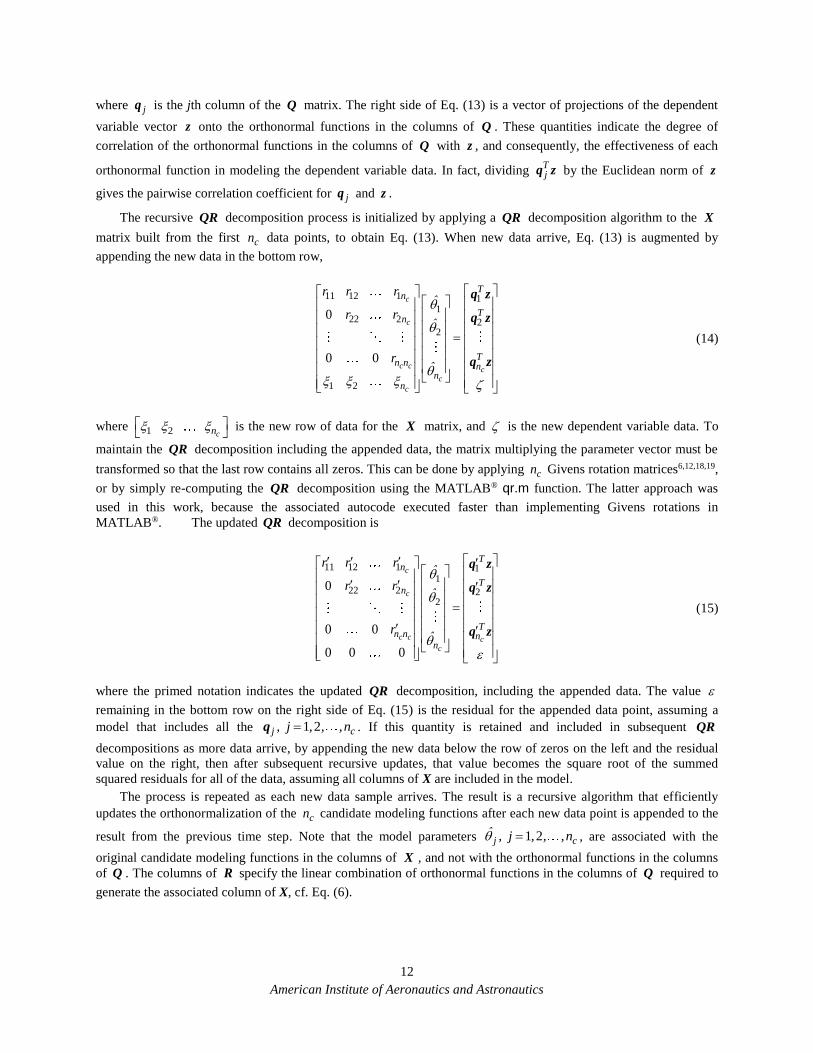
The recursive QR decomposition process is initialized by applying a QR decomposition algorithm to the X
matrix built from the first cn data points, to obtain Eq. (13). When new data arrive, Eq. (13) is augmented by
appending the new data in the bottom row,
11 12 1 11
22 2 22
1 2
0
0 0
c
c
c cc
c
c
Tn
Tn
Tn n n
nn
r r rˆ
r rˆ
rˆ
q z
q z
q z
(14)
where 1 2 cn
is the new row of data for the X matrix, and is the new dependent variable data. To
maintain the QR decomposition including the appended data, the matrix multiplying the parameter vector must be
transformed so that the last row contains all zeros. This can be done by applying cn Givens rotation matrices6,12,18,19,
or by simply re-computing the QR decomposition using the MATLAB® qr.m function. The latter approach was
used in this work, because the associated autocode executed faster than implementing Givens rotations in
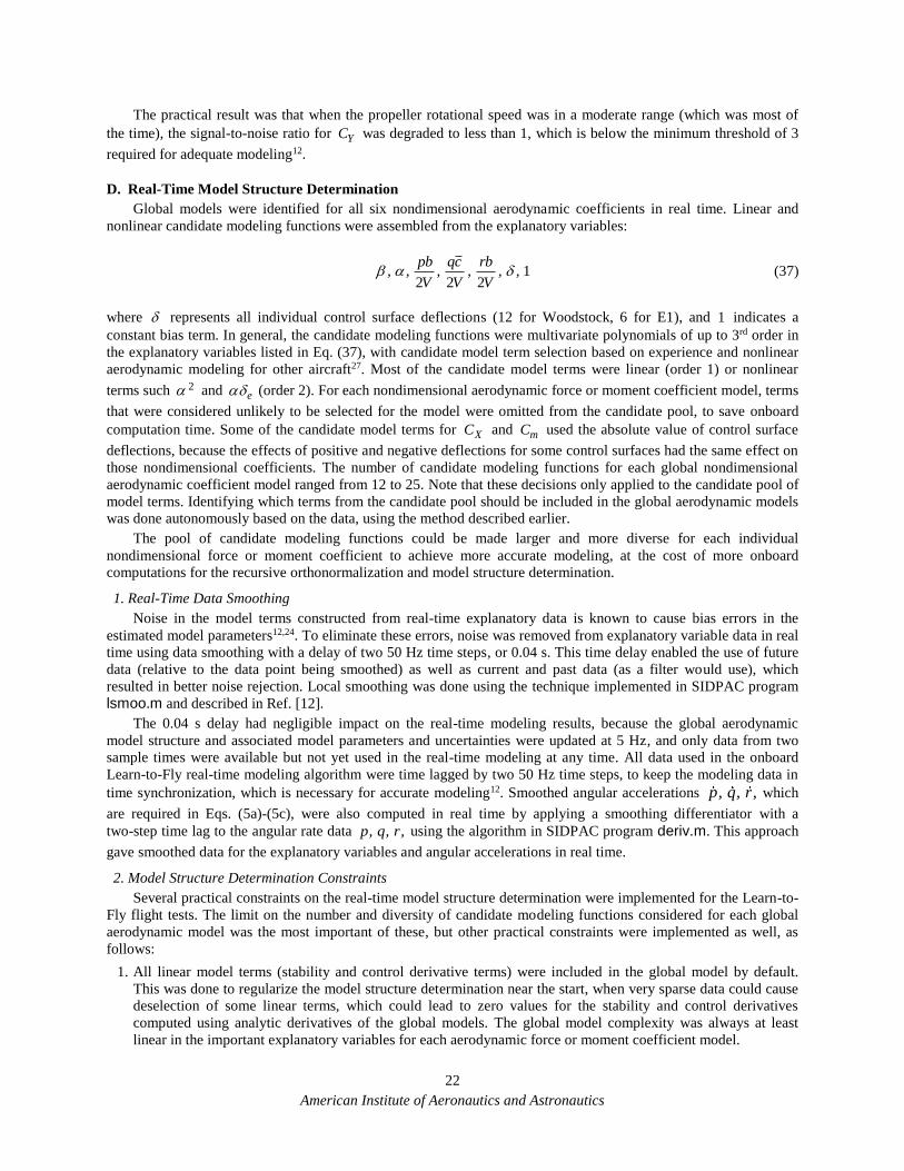
MATLAB®. The updated QR decomposition is
11 12 1 11
22 2 22
0
0 0
0 0 0
c
c
c c cc
Tn
Tn
Tn n n
n
r r rˆ
r rˆ
rˆ
q z
q z
q z
(15)
where the primed notation indicates the updated QR decomposition, including the appended data. The value
remaining in the bottom row on the right side of Eq. (15) is the residual for the appended data point, assuming a
model that includes all the 1 2j c, j , , ,nq . If this quantity is retained and included in subsequent QR
decompositions as more data arrive, by appending the new data below the row of zeros on the left and the residual
value on the right, then after subsequent recursive updates, that value becomes the square root of the summed
squared residuals for all of the data, assuming all columns of X are included in the model.
The process is repeated as each new data sample arrives. The result is a recursive algorithm that efficiently
updates the orthonormalization of the cn candidate modeling functions after each new data point is appended to the
result from the previous time step. Note that the model parameters 1 2j cˆ , j , , ,n , are associated with the
original candidate modeling functions in the columns of X , and not with the orthonormal functions in the columns
of Q . The columns of R specify the linear combination of orthonormal functions in the columns of Q required to
generate the associated column of X, cf. Eq. (6).

American Institute of Aeronautics and Astronautics
13
2. Least Squares Parameter Estimation using Orthonormal Functions
The form of a model using orthonormal modeling functions is
1 1 2 2 n na a ... a z q q q (16)
where z is an N-dimensional vector of dependent variable data (e.g., nondimensional force or moment coefficient
data), 1 2T
Nz ,z ,...,zz , modeled in terms of a linear combination of n mutually orthonormal modeling functions
1 2j , j , ,...,nq . Each jq is an N-dimensional vector that in general depends on the explanatory variables. The
1 2ja , j , ,...,n are unknown constant model parameters to be determined, and denotes the modeling error vector.
Assembling the n orthonormal modeling functions from Eq. (16) in the columns of an N n matrix Q ,
1 2 n, , ...,
Q q q q (17)
and defining the unknown parameter vector 1 2T
na ,a ,...,aa , Eq. (16) can be written as
z Qa ε (18)
which is the same equation discussed earlier in Eq. (8), except that the modeling functions are now orthonormal
functions. In this case, it is easier to determine an appropriate model structure, because the explanatory capability of
each of the modeling functions in the columns of Q is completely distinct from all of the others, due to the mutual
orthogonality. This decouples the least squares modeling problem, as will be shown now.
For mutually orthonormal functions,
1 for
1 20 for
Ti j
i ji, j , , ...,n
i j
q q (19)
and T
Q Q is the identity matrix. Using Eq. (19) in the least-squares solution from Eq.(10c) for the model in
Eq. (18), the jth element of the estimated parameter vector a is
Tj ja q z (20)
The least-squares cost function using orthonormal functions is then
2
1
1 1
2 2
nT T T T
j
j
ˆ ˆ ˆJ
a z z a a z z q z (21)
Equation (21) shows that when the modeling functions are orthonormal, the reduction in the least-squares cost
function resulting from including the term j ja q in the model depends only on the dependent variable data z and the
added orthonormal modeling function jq . The least-squares modeling problem is therefore decoupled, which means
each orthonormal modeling function can be evaluated independently in terms of its ability to reduce the least-
squares model fit to the data, regardless of which other orthonormal modeling functions are already selected for the
model. If the modeling functions were instead polynomials in the explanatory variables (or any other non-orthogonal
function set), then the least-squares problem would be coupled and iterative analysis would be required to find a

American Institute of Aeronautics and Astronautics
14
subset of the candidate modeling functions for an adequate model structure. The orthogonalization removes the need
for this iteration, and therefore makes the model structure determination feasible in real time.
The vector on the right side of Eq. (15) from the recursive QR decomposition contains exactly the quantities
Tjq z appearing in Eqs. (20) and (21). These quantities are calculated for all cn candidate modeling functions, and
are used to identify the model structure, which involves selecting the functions to be included in the model from the
pool of cn candidate modeling functions.
C. Modeling Metrics
Statistical modeling metrics were used to select which of the orthonormal candidate modeling functions should
be included in the model for each nondimensional aerodynamic force or moment coefficient. The modeling metrics
were:
1. Coefficient of determination 2R
2 2
2 1 12
2 2
1 1
1 1
zz y z y
z z zz z
N N
T
i iN N T
i i
ˆ ˆy i z i y iˆ ˆ
RN
z i z i
(22)
The 2R metric12 quantifies the fraction of the variation in the dependent variable about its mean that is explained by
the model, so that 20 1R . Often, 2R is given as a percentage.
2R is a model fit quality measure.
2. Predicted Squared Error PSE
21 T
max
nˆ ˆPSEN N
z Xθ z Xθ (23)
or
22max
nˆPSE JN N
θ (24)
The PSE metric12,25 quantifies the expected squared prediction error for an identified model when applied to
data not used in the model identification process. The constant 2max is an upper-bound estimate of the dependent
variable noise variance. The PSE metric is a combination of a model fit quality measure (the first term on the right
side of Eq. (24), the mean squared fit error, proportional to the least-squares cost function) and a model complexity
penalty (the second term on the right side of Eq. (24), proportional to the number of terms in the model, n).
Reference [25] contains statistical arguments and analysis for the PSE metric, including justification for its use in
modeling problems.
To compute the preceding model metrics, each orthonormal candidate modeling function being evaluated for
inclusion in the model must be tentatively included, or tried out, in the model. The recursive QR decomposition for
all orthonormal candidate modeling functions does this automatically, in a way that facilitates evaluation and
selection of modeling functions in real time.
D. Real-Time Model Structure Determination using Orthonormal Functions
The orthonormal modeling functions to be included in the model were chosen to minimize the predicted squared
error metric PSE defined in Eq. (23),
21 Tmax
nˆ ˆPSE
N N z Qa z Qa (25)

American Institute of Aeronautics and Astronautics
15
Combining Eq. (25) with Eqs. (24) and (21),
2
2
1
1n
T Tj max
j
nPSE
N N
z z q z (26)
An estimate of 2max that is independent of the model structure can be obtained in real time by computing a
running average of squared values from a high-pass filter applied to the dependent variable data. This real-time
estimate of the noise variance for the dependent variable can then be multiplied by a factor to implement a
conservative estimate for the upper bound 2max . In the Learn-to-Fly work, a second-order Butterworth high-pass
filter with break frequency set at 3 Hz was applied to the real-time dependent variable data, and the result was
squared and averaged in real time. This mean square value was then multiplied by a factor of 25 to obtain a
conservative estimate of 2max (corresponding to 5 times the estimated standard deviation),
2 2 211i i iˆ ˆi v i
(27a)
2 225 or 5 max maxˆ ˆ ˆ ˆ (27b)
where iv is the high-pass filtered dependent variable data at the ith time step.
Using a conservative upper bound estimate for 2max means the PSE metric will tend to overestimate actual
squared prediction errors for new data. Therefore, the PSE metric conservatively estimates the squared error for
prediction cases. Other high-pass filter designs and break frequencies could be used as well. The purpose of the
high-pass filter design is to isolate the components of the dependent variable data that characterize the magnitude of
the noise for model structure determination purposes.
The last term on the right in Eq. (26) prevents overfitting the data with too many model terms, which is
detrimental to model prediction accuracy12,25. The mean squared fit error must decrease with the addition of each
orthonormal modeling function to the model (because 2
Tj q z is always negative, and
Tz z is unaffected by the
model), whereas the overfit penalty term 2max n N must increase with each added model term (n increases). The
recursive QR decomposition described earlier computes Tjq z for each of the orthonormal candidate modeling
functions 1 2j c, j , ,...,nq at each time step.
Because the quantities T
z z , 2max , and N depend only on the dependent variable data, and therefore cannot be
altered by the model, Eq. (26) shows that the criterion for including each jq in the model based on minimizing PSE
can be reduced to
2
2Tj maxq z (28)
The criterion in Eq. (28) is a mathematical statement of the simple physical idea that only orthonormal
modeling functions that reduce the squared fit error by an amount that exceeds the maximum expected noise
variance should be included in the model. This is the condition necessary for PSE to decrease when jq is added to
the model.
Using orthonormal functions to model the dependent variable data makes it possible to evaluate the merit of
including each modeling function individually, based on the PSE metric. The goal is to select a model structure with
minimum PSE, and the PSE will always have a single global minimum for the model that includes only the

American Institute of Aeronautics and Astronautics
16
orthonormal modeling functions that satisfy Eq. (28). Model structure determination based on the PSE metric is
therefore a well-defined and straightforward process that can be (and was) automated.
In addition to the PSE criterion, each selected orthonormal function jq was required to model at least a selected
fraction of the total variation about the mean for the dependent variable, quantified by the change in the 2R metric
resulting from adding jq to the model,
2
2
Tj
minTR
N
q z
z z z (29)
This can be computed from the results of the recursive QR decomposition and simple real-time calculations using
the dependent variable data,
11i i ii z i z z (30)
2
1
T Ti
i iz
z z z z (31)
For the Learn-to-Fly work, 2minR was selected as 0.005, which corresponds to requiring each selected
orthonormal function to model at least 0.5 percent of the total variation in the dependent variable about the mean.
Finally, a check for data information deficiency in the columns of X was done, by ensuring that the sum of the
values in each column of R was greater than a numerical zero tolerance, set at 10-5. This ensured that each of the
original candidate modeling functions in X could be expressed in terms of the orthonormal modeling functions being
evaluated for inclusion in the model. For any column of R that did not meet this criteria, the associated column of X
was unnecessary (redundant), and that model term was excluded from the model by setting the associated model
parameter estimate to zero.
Model parameters associated with the original candidate modeling functions in the columns of the X matrix
were determined from Eq. (12), using all rows and columns of the R matrix up to and including the index
associated with the last element of vector T
Q z selected for the model. Because the orthonormalization of the
multivariate functions in the X matrix is done in the order of the columns in X , all prior rows and columns of ˆRθ
must be included in the calculation of the model parameter estimates for each selected jq . Accordingly, if the last
element of vector T
Q z selected for the model is element m, only the elements 1 2jˆ , j , , ,m are estimated – the
remaining elements of θ are associated with candidate modeling functions that were not selected for the model, and
were not involved in the orthonormalization of the selected orthonormal functions, so those parameters are zero.
The identified model output can be computed from
m mˆy X θ (32)
where mX and mθ include only the first m columns of X and elements of θ , respectively, and m is highest value
of j for the orthonormal modeling functions selected for the model, or equivalently, the number of the last T
Q z
vector element selected for the model. Note that
cn m n (33)

American Institute of Aeronautics and Astronautics
17
because the number of orthonormal functions selected for the model, n, can be less than the highest index for
selected orthonormal modeling functions, m, and both of these values can be (and usually are) less than the total
number of candidate modeling functions, cn .
1. Model Parameter Uncertainty
Model parameter uncertainty can be found from12
1
2 Tm m mˆ
Σ θ R R (34)
where mR includes only the first m rows and columns of R , and m is the index associated with the last selected
model term from vector T
Q z . The fit error variance assuming all cn candidate modeling functions are included in
the model comes from the square of the lower right value in Eq. (15) after each recursive QR decomposition
update. When cn n modeling functions are selected for the model (the usual case), the squared residual estimate
must be augmented with the squared residual associated with the modeling functions that were not selected for the
model. This is easy to compute, because the fit error variance reduction associated with each omitted jq function is
simply 2
Tjq z , from Eq. (26). The fit error variance computed from the lower right element in Eq. (15) is simply
augmented by adding 2
Tjq z for each jq not selected for the model. Finally, corrections for colored residuals can
be made post-flight12 or using real-time estimates of the residual autocorrelation function12,26.
2. Practical Issues
The orthonormalization of candidate modeling functions has a sequence dependence, in that the
orthonormalization changes if the order of the candidate modeling functions in the columns of X is changed. This
can reduce the number of terms in the final model, because each orthonormal function in general depends on
original candidate modeling functions in prior columns of X , because the R matrix is upper triangular.
Consequently, a model with the smallest number of model terms will be identified when all of the selected
orthonormal functions were first in line for orthonormalization.
It is possible to re-order the orthonormal modeling functions by exchanging rows and columns of the R matrix,
then updating the QR factorization. Moving the candidate modeling functions that are identified as important to the
front of the orthogonalization sequence means that interim unselected candidate model terms do not need to be
included in the final model. This results in a reduced number of functions in the model, because the number of rows
of R needed for the selected orthonormal modeling functions is reduced. However, this feature was not
implemented for Learn-to-Fly real-time modeling, because it required too much computation and bookkeeping for
real-time operation. Instead, the order of the columns in the X matrix, and therefore also the order of the rows and
columns in the R matrix, remained fixed and determined by an initial prescribed ordering of the candidate
modeling functions in the X matrix.
The recursive orthonormalization and automated model structure determination identifies which model terms
from the candidate pool are necessary to characterize the functional dependencies, and estimates the associated
model parameters and uncertainties. Because the approach is based on time-domain equation-error modeling, if data
points are missed because of instrumentation or telemetry malfunctions, the modeling algorithm is unaffected
(except for any loss of information in the missed data points), because the equation-error approach in the time-
domain does not depend on the time sequence of the data. Therefore, gaps in the real-time data stream can be
tolerated without modification to the algorithm. However, large data values associated with dropouts will adversely
affect the modeling, as is the case for all time-domain modeling methods. The real-time data smoothing described
earlier effectively removes isolated data dropouts, but the Learn-to-Fly modeling algorithm also monitored
magnitudes of the explanatory and dependent variable data, and skipped any data points where reasonable practical
limits were exceeded. Skipping bad data points has a small effect on real-time data smoothing, filtering, and smooth
numerical differentiation, but no detrimental effects on the modeling algorithm calculations. This is a significant
advantage for real-time operation, and was one reason that Learn-to-Fly real-time global aerodynamic modeling was
based on the time-domain equation-error approach.

American Institute of Aeronautics and Astronautics
18
In general, there are no restrictions regarding the form of the candidate modeling functions - they can be
multivariate polynomials, multivariate spline functions, or any other linear or nonlinear function that can be
computed from the explanatory variable data. Inputs required from the analyst relate only to the limits of what
should be considered, such as which explanatory variables to consider, the maximum order of multivariate
polynomial functions to consider, spline knot locations, and so on. Obviously, the accuracy and prediction capability
of each identified model depends on the pool of candidate modeling functions available for selection. The number of
candidate modeling functions that were available for the real-time global modeling implemented in Learn-to-Fly
was constrained by computational limitations of the onboard flight computer. These limitations were affected by the
other real-time Learn-to-Fly tasks running concurrently on the onboard flight computer, such as real-time control
and real-time guidance. Real-time global modeling for the six nondimensional force and moment coefficients
employed a unique and separate pool of candidate modeling functions for each model, with associated separate
recursive orthonormalizations. Additional onboard computation capability would enable more accurate and
complete global modeling results, because a larger and more diverse pool of candidate modeling functions could be
considered.
For any pool of candidate modeling functions, the real-time modeling algorithm uses the same approach to
automatically sort out which of the candidate modeling functions are important, based on the data, and selects only
those for the model. The result is a global parsimonious model that characterizes the functional dependencies
accurately and predicts well.
V. Learn-to-Fly Real-Time Modeling Flight Test Results
Flight testing was conducted at Fort A.P. Hill Army base near Bowling Green, VA, using the instrumented
Woodstock and E1 aircraft shown in Figs. 3 and 4 and described in Section II. References [13] and [14] provide an
overview of the Learn-to-Fly project and associated flight testing. Details of the real-time control and real-time
guidance algorithms used in Learn-to-Fly flight testing can be found in Refs. [15] and [16], respectively.
A. Flight Test Implementation
The data conditioning for real-time modeling, including real-time smoothing for the explanatory variables, real-
time smooth differentiation, high-pass filtering to obtain real-time estimates of the noise variance for the
nondimensional force and moment coefficients, and recursive orthogonalization of the candidate modeling
functions, was done onboard the aircraft at 50 Hz. Model structure determination, model parameter estimation, and
model parameter uncertainty calculations were done at a slower 5 Hz rate using a separate computational thread in
the onboard flight computer. This arrangement was necessary because other real-time operations such as real-time
guidance and control, data acquisition, and data logging were done at 50 Hz, and the onboard computational
capability was not sufficient to do everything in a 50 Hz time frame without frame overflows. Separating the
modeling structure determination, model parameter estimation, and model parameter uncertainty calculations from
the other real-time modeling calculations was fairly straightforward, and the penalty incurred was that the global
model updates would be done at a slower 5 Hz rate. However, this was not a significant penalty, because global
aerodynamic functional dependencies for rigid-body aircraft rarely change faster than about 2 Hz, except for sudden
failures, highly nonlinear flight regimes, and/or rapid maneuvering. Arranging the onboard calculations in this way
allowed all of the necessary real-time modeling calculations to be made within the 50 Hz and 5 Hz time frames,
while the other Learn-to-Fly components operated at 50 Hz.
Even with the separation of real-time modeling calculations into two computational threads, achieving real-time
global modeling onboard the aircraft was a computational challenge, wherein the true nonlinear functional
dependencies were approximated by a necessarily finite set of linear and nonlinear functions of the explanatory
variables. The result was a compromise of global modeling capability in terms of the number and variety of
candidate modeling functions that could be considered for each model. This issue impacted the robustness needed in
the control law, requiring a complex balance between desired control law performance, changing real-time modeling
accuracy that depended on time-varying data information, and the degree of modeling fidelity possible with a finite
number of relatively simple functions of the explanatory variables and noisy flight data.
A characteristic of real-time modeling that was particularly important for Learn-to-Fly is the fact that real-time
modeling is an analytic process, and not a predictive process. Aerodynamic dependencies must first be sufficiently
exhibited in the data before real-time modeling can accurately characterize those dependencies. Practically, this
means that real-time modeling results always have a slight time lag because of the need to collect enough data to
make accurate judgments about the dependencies. This issue does not arise for conventional modeling based on data

American Institute of Aeronautics and Astronautics
19
from entire maneuvers. Consequently, part of the flight testing for Learn-to-Fly involved the timing for data
collection, PTI excitation, real-time modeling results, and learning adaptive control initiation.
When each Learn-to-Fly flight test run was initiated, a period of time was allowed for the aircraft to recover
from the initial condition and stabilize at a nominal flight condition, using a simple and robust recovery control law.
Then modeling data collection started, followed by PTI excitations on all control surfaces individually and
simultaneously. After a short period of time, the real-time modeling algorithm began producing real-time modeling
results for use by other components of the Learn-to-Fly algorithm. A short time after real-time modeling outputs
began, learning adaptive control was initiated. A typical flight test time line is shown in Fig. 8. Both the excitation
and the real-time modeling continued until the safety pilot manually shut them off, or until the aircraft flew below a
specified altitude to set up for approach and landing.
Figure 8. Learn-to-Fly flight test timeline
B. Real-Time Local Linear Models
Local linear model parameters were computed in real time from the identified global aerodynamic models,
using analytic derivatives evaluated at the current aircraft measured states and controls. Analytic derivatives were
computed automatically, because the mathematical forms of the candidate modeling functions were known. Real-
time linear aerodynamic model parameters, which are nondimensional stability and control derivatives, were
evaluated using 50 Hz real-time data for aircraft states and controls, although the global models that were
analytically differentiated were updated at 5 Hz. The higher 50 Hz rate for real-time stability and control derivatives
was implemented for better accuracy and more effective real-time learning adaptive control.
All real-time modeling results have an inherent variability that arises from time-varying data information,
measurement noise, and model structure errors. To mitigate this variability, and to provide smoother local linear
modeling information to the real-time learning adaptive control, simple real-time low-pass filtering was applied to
the real-time local modeling results produced at 50 Hz. The low-pass filtering was implemented using a weighted
average of the current estimate and the most recent filtered value for local modeling results. The resulting filtered
values were broadcast to the other components of the Learn-to-Fly algorithm and recorded. For example, the current
filtered estimate of the pitching moment static stability derivative mC i
was computed from
1 21m m mˆC i w C i w C i
(35)
where mC i
was the local derivative of the current global mC model with respect to , evaluated at current
conditions, mC i
was the filtered value broadcast to other parts of the Learn-to-Fly algorithm as the current
estimate of mC
, and 1mC i
was the most recent past value of mC
. The weightings were chosen as
1 20 5 0 5w . w . (36a)

American Institute of Aeronautics and Astronautics
20
Higher values of 1w would produce smoother results with more time lag, whereas higher values of 2w would
produce more variable results with less time lag. To implement a weighted average, the weightings must satisfy
1 2 1 0w w . (36b)
Note that the immediate past value of a local linear real-time estimate (such as 1mC i
in Eq. (35)) includes data
information from a stretch of time into the past. This real-time low-pass filtering was applied only to the local linear
model parameters (stability and control derivatives), and not to the global model parameters. The filtered linear
model results were used to compute local linear dynamic model matrices at 50 Hz, which were also broadcast to the
other components of the Learn-to-Fly algorithm.
At the start of a Learn-to-Fly test run, there was no information about the aircraft aerodynamics, but rough
guesses for the stability and control derivatives, based on a conventional aircraft with similar size, were
implemented as initial linear aerodynamic model parameters. This was done so that other components of the Learn-
to-Fly algorithm would have something to use initially, before sufficient data were collected for real-time modeling
results, and also to make the transition from no information to real-time modeling information less abrupt. Because
of the low-pass filtering described earlier, the real-time modeling results for stability and control derivatives
transitioned smoothly and quickly from the initial guesses to real-time estimates computed from the data. Linear
terms in the global model were initialized in the same way for similar reasons, but did not have low-pass filtering.
C. Data Information Content
Accurate modeling based on experimental data requires uncorrelated excitation of the explanatory variables,
with sufficient amplitude so that the deterministic aircraft response is significantly larger than the noise levels. To
that end, Learn-to-Fly flight tests involved excitations on all control surfaces simultaneously, to collect
comprehensive and informative data quickly. Such excitations intentionally cause dynamic responses from the
aircraft, which are required to produce informative data for real-time modeling. Unfortunately, this is at odds with
one goal of feedback control laws, which is disturbance rejection. During Learn-to-Fly flights, this can cause a
conflict, because control surface excitations must be allowed so that real-time modeling has good data information
quickly, but the control law sees the resulting dynamic responses as disturbances that must be squelched. The irony
is that the more successful the control law is in squelching the dynamic response in the short term, the worse the
control law will be in the longer term, because the control law depends on an accurate model, and the model will
only be accurate if the dynamic response of the aircraft from control surface excitations is allowed, so that real-time
modeling has the data information required to work properly.
Any degradation of the excitation inputs adversely impacts data information content and therefore also degrades
real-time modeling effectiveness and accuracy. Learning adaptive control used a sophisticated algorithm to achieve
real-time control, based on both global and local real-time modeling results15. Figure 9 shows typical distortion of
the PTI excitations in the frequency domain, for the E1 aircraft with learning adaptive control active. The
differences shown include both PTI distortion by the learning adaptive control, as well as control surface deflections
resulting from real-time guidance commands. The learning adaptive control law had a significant impact on the
rudder excitation, as well as the low-frequency elevator and aileron excitations. This degraded the data information
content for real-time modeling, but the input design was robust to these distortions, and the resulting flight data still
had sufficient data information content for good real-time modeling results. The real-time learning adaptive control
implemented in Learn-to-Fly was operating with relatively high gain in parts of the same frequency range as the
excitation inputs, and therefore squelched a portion of the excitations.
Remediation for this problem might be allocating specific frequencies for the PTI and keeping those frequencies
separate from the frequencies allowed for the learning adaptive control, or reducing the feedback gains while the
PTI and real-time modeling are active, or simply applying the PTI with a simpler low-gain control law until the real-
time model is identified to a desired accuracy, then switching to learning adaptive control for precision guidance and
maneuvering.
For any modeling, the signal-to-noise ratio for the dependent variable is critically important. The E1 aircraft had
a propeller and a relatively lightweight structure, which resulted in significantly degraded signal-to-noise ratios for
the nondimensional aerodynamic coefficients at some propeller rotational speeds. Figure 10 shows an example from
E1 flight 6, where the measured translational accelerations (directly related to the nondimensional aerodynamic
force coefficients, cf. Eq. (4)), were much noisier when the propeller rotational speed fell within a moderate range
commonly used throughout the flight testing. Propeller rotational speeds either substantially higher or lower than

American Institute of Aeronautics and Astronautics
21
this moderate range resulted in lower noise levels, suggesting that some aircraft structural dynamic response was
excited.
Figure 9. E1 excitation input distortion for learning adaptive control
Figure 10. E1 flight 6 noise levels for varying propeller rotational speeds
ra
r
rf
lf
la
e
g
xa
rpm
p
g
ya
g
za
6000
4000
2000
0
American Institute of Aeronautics and Astronautics
22
The practical result was that when the propeller rotational speed was in a moderate range (which was most of
the time), the signal-to-noise ratio for YC was degraded to less than 1, which is below the minimum threshold of 3
required for adequate modeling12.
D. Real-Time Model Structure Determination
Global models were identified for all six nondimensional aerodynamic coefficients in real time. Linear and
nonlinear candidate modeling functions were assembled from the explanatory variables:
12 2 2
pb qc rb, , , , , ,
V V V (37)
where represents all individual control surface deflections (12 for Woodstock, 6 for E1), and 1 indicates a
constant bias term. In general, the candidate modeling functions were multivariate polynomials of up to 3rd order in
the explanatory variables listed in Eq. (37), with candidate model term selection based on experience and nonlinear
aerodynamic modeling for other aircraft27. Most of the candidate model terms were linear (order 1) or nonlinear
terms such 2 and e (order 2). For each nondimensional aerodynamic force or moment coefficient model, terms
that were considered unlikely to be selected for the model were omitted from the candidate pool, to save onboard
computation time. Some of the candidate model terms for XC and mC used the absolute value of control surface
deflections, because the effects of positive and negative deflections for some control surfaces had the same effect on
those nondimensional coefficients. The number of candidate modeling functions for each global nondimensional
aerodynamic coefficient model ranged from 12 to 25. Note that these decisions only applied to the candidate pool of
model terms. Identifying which terms from the candidate pool should be included in the global aerodynamic models
was done autonomously based on the data, using the method described earlier.
The pool of candidate modeling functions could be made larger and more diverse for each individual
nondimensional force or moment coefficient to achieve more accurate modeling, at the cost of more onboard
computations for the recursive orthonormalization and model structure determination.
1. Real-Time Data Smoothing
Noise in the model terms constructed from real-time explanatory data is known to cause bias errors in the
estimated model parameters12,24. To eliminate these errors, noise was removed from explanatory variable data in real
time using data smoothing with a delay of two 50 Hz time steps, or 0.04 s. This time delay enabled the use of future
data (relative to the data point being smoothed) as well as current and past data (as a filter would use), which
resulted in better noise rejection. Local smoothing was done using the technique implemented in SIDPAC program
lsmoo.m and described in Ref. [12].
The 0.04 s delay had negligible impact on the real-time modeling results, because the global aerodynamic
model structure and associated model parameters and uncertainties were updated at 5 Hz, and only data from two
sample times were available but not yet used in the real-time modeling at any time. All data used in the onboard
Learn-to-Fly real-time modeling algorithm were time lagged by two 50 Hz time steps, to keep the modeling data in
time synchronization, which is necessary for accurate modeling12. Smoothed angular accelerations p, q, r, which
are required in Eqs. (5a)-(5c), were also computed in real time by applying a smoothing differentiator with a
two-step time lag to the angular rate data p, q, r, using the algorithm in SIDPAC program deriv.m. This approach
gave smoothed data for the explanatory variables and angular accelerations in real time.
2. Model Structure Determination Constraints
Several practical constraints on the real-time model structure determination were implemented for the Learn-to-
Fly flight tests. The limit on the number and diversity of candidate modeling functions considered for each global
aerodynamic model was the most important of these, but other practical constraints were implemented as well, as
follows:
1. All linear model terms (stability and control derivative terms) were included in the global model by default.
This was done to regularize the model structure determination near the start, when very sparse data could cause
deselection of some linear terms, which could lead to zero values for the stability and control derivatives
computed using analytic derivatives of the global models. The global model complexity was always at least
linear in the important explanatory variables for each aerodynamic force or moment coefficient model.

American Institute of Aeronautics and Astronautics
23
2. Model terms involving control surfaces that appeared in pairs on the aircraft (such as left and right aileron) were
only chosen for global models when the terms for both control surfaces passed the statistical tests for inclusion
in the model. This avoided transient selections of only one of the terms associated with a pair of control surfaces
for any global model, which caused problems for the control allocation in the real-time control law.
3. Selected model terms were latched, so that once a particular model term passed the statistical tests for inclusion
in the global model, that model term stayed in the global model. This prevented transient selection and
deselection of model terms, which could cause discontinuities in the real-time stability and control derivative
estimates.
The E1 aircraft has a propeller driven by an electric motor, which means that the applied force in the body-axis
x direction, XF , included both thrust and aerodynamic forces. A global model for XF would require additional
candidate model terms to characterize the thrust, such as linear and nonlinear terms involving the propeller advance
ratio. Unfortunately, the development schedule for the E1 aircraft was highly compressed, and there was not enough
time to implement and validate the necessary modifications to the real-time modeling algorithm to change XC
global aerodynamic modeling (developed for the Woodstock glider) to XF global modeling for combined
aerodynamics and thrust. In addition, data from the sensor for propeller rotational speed on the E1 aircraft was not
calibrated and produced questionable data. Therefore, the real-time global modeling for XC on the E1 aircraft was
invalid. The real-time modeling still attempted to model XC with the model terms available, but because the
available model terms did not include terms involving the propeller advance ratio, and the XC
nondimensionalization was not correct for the thrust, the global models identified for XC from E1 flight data were
poor.
Apart from the thrust modeling issue, real-time modeling for Learn-to-Fly can be converted from one aircraft to
another by simply changing the number of controls and adjusting the candidate modeling function pools
accordingly. This was successfully demonstrated when transitioning the Learn-to-Fly real-time modeling from
Woodstock to E1, except for XC modeling.
E. Real-Time Global Modeling
Figures 11 and 12 show real-time global aerodynamic modeling results from E1 flight 3 with PTI active, but no
learning adaptive control. The safety pilot was flying the aircraft using conventional radio-control commands, with
PTI excitations added autonomously to all individual control surface commands simultaneously. Modeling results
for XC and YC are not shown, because the XC model was invalid from not incorporating thrust modeling terms,
and the YC signal-to-noise ratio was very low, because of high noise levels induced at moderate propeller rotational
speeds. However, the onboard real-time modeling still attempted to identify global models for XC and YC , and
those results were broadcast to other components of the Learn-to-Fly algorithm, along with the results for the other
nondimensional force and moment coefficient models shown in Figs. 11 and 12. Fortunately, the XC and YC
models have relatively minor importance for aircraft stability and control.
The plots in Fig. 11 show the longitudinal global model fits to flight data in real time. The top plot is the global
model fit for ZC , and the plot below that shows the residual or difference between the data and the model. The third
and fourth plots in Fig. 11 are analogous plots for mC . Because the identified global models were updated
continually and recorded, model prediction capability can be examined post-flight. The traces to the left of the
vertical lines in the plots represent model fit to the data collected up to that point, using the real-time global models
identified at the time marked by the vertical lines. The traces to the right of the vertical lines represent a 20-second
prediction using the real-time global models identified at the time marked by the vertical lines. The prediction
residuals to the right of the vertical lines have approximately the same magnitude and character as the modeling
residuals to the left of the vertical lines. This indicates accurate global model identification with good prediction
capability.
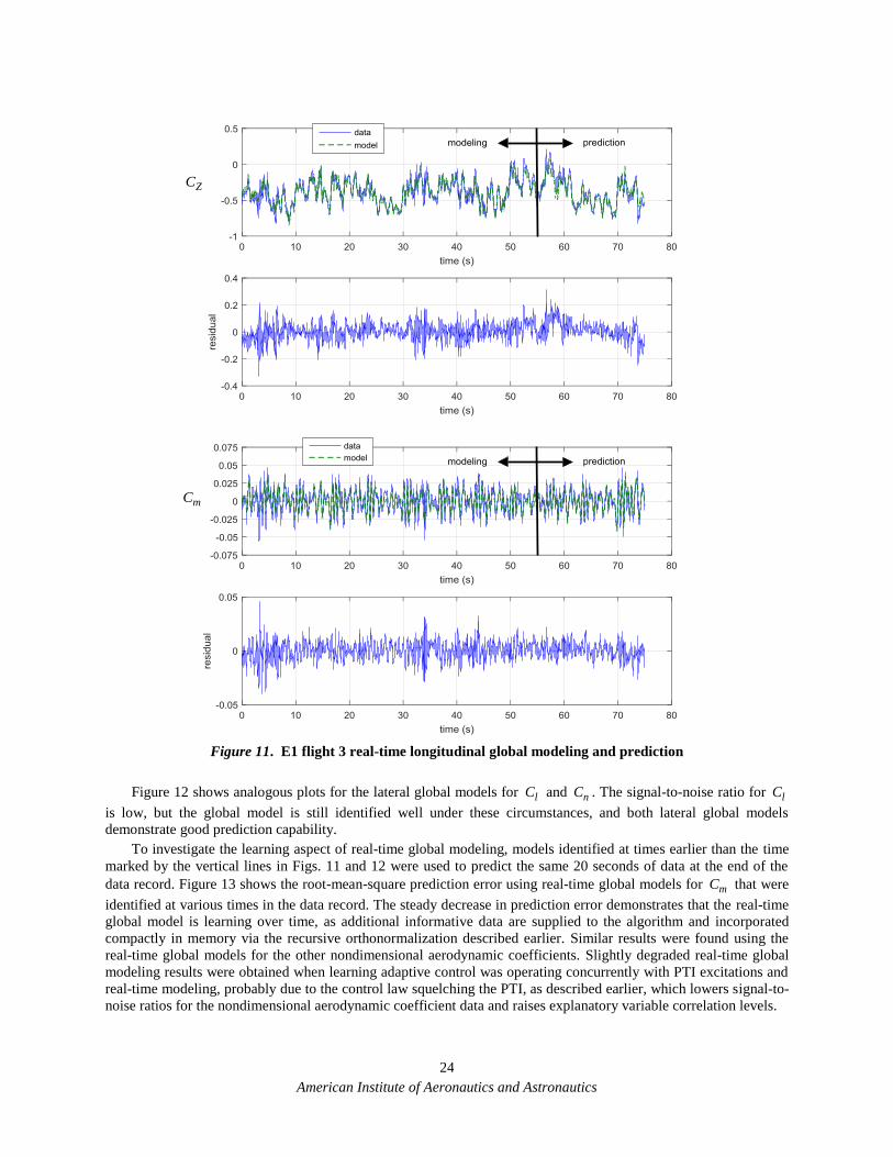
American Institute of Aeronautics and Astronautics
24
Figure 11. E1 flight 3 real-time longitudinal global modeling and prediction
Figure 12 shows analogous plots for the lateral global models for lC and nC . The signal-to-noise ratio for lC
is low, but the global model is still identified well under these circumstances, and both lateral global models
demonstrate good prediction capability.
To investigate the learning aspect of real-time global modeling, models identified at times earlier than the time
marked by the vertical lines in Figs. 11 and 12 were used to predict the same 20 seconds of data at the end of the
data record. Figure 13 shows the root-mean-square prediction error using real-time global models for mC that were
identified at various times in the data record. The steady decrease in prediction error demonstrates that the real-time
global model is learning over time, as additional informative data are supplied to the algorithm and incorporated
compactly in memory via the recursive orthonormalization described earlier. Similar results were found using the
real-time global models for the other nondimensional aerodynamic coefficients. Slightly degraded real-time global
modeling results were obtained when learning adaptive control was operating concurrently with PTI excitations and
real-time modeling, probably due to the control law squelching the PTI, as described earlier, which lowers signal-to-
noise ratios for the nondimensional aerodynamic coefficient data and raises explanatory variable correlation levels.
ZC
mC

American Institute of Aeronautics and Astronautics
25
Figure 12. E1 flight 3 real-time lateral global modeling and prediction
Figure 13. E1 flight 3 real-time global mC model learning based on 20-second prediction error
lC
nC
rms prediction error
mC

American Institute of Aeronautics and Astronautics
26
For the real-time global modeling implemented in Learn-to-Fly, conventional model parameter uncertainties
were computed, as described earlier. However, these uncertainty calculations are based on asymptotic properties and
the implicit assumption that data from an entire maneuver are available for both the modeling and the model fit error
variance estimation. In the Learn-to-Fly context, modeling results and model parameter uncertainty measures are of
interest early in the data collection process and at interim times thereafter, which is a very different requirement
compared to conventional modeling. Using prediction error rather than conventional statistical uncertainty measures
could be more practical and accurate for real-time modeling, but this will require further study.
Traditional control law design is based on an assumed model that does not change with time. In a Learn-to-Fly
flight, the model is changing continually, as real-time global modeling improves as a result of informative data being
collected over time. Consequently, the control law cannot be static, but rather must adapt to a model that is
improving with time, while also being robust to inaccuracies in the model early in the flight. This can be done by
relaxing controller performance requirements early in the Learn-to-Fly flight, when the real-time modeling is still
has much to learn, then tightening the performance requirements as the flight progresses and the real-time modeling
improves based on additional informative data. As the Learn-to-Fly flight progresses, the real-time modeling
becomes more comprehensive and accurate, and ultimately the real-time guidance and control must be able to
successfully execute the approach and landing tasks. Learning adaptive control and real-time guidance must be able
to use modeling results that not only change and improve in accuracy sequentially with time, but can also have local
stochastic variations in time, as a result of using noisy flight data.
Conventional aerodynamic modeling from flight data is typically done by executing a flight test maneuver, then
analyzing the data from the entire maneuver. This makes sense for practical reasons, and also because a full
maneuver allows time for the dynamic response of the aircraft to be exhibited clearly and completely in the data. For
real-time modeling, interim modeling results are of interest, which means that modeling results are desired when the
data collection is incomplete, consisting of only partial periods of the dominant dynamic modes, or data confined to
a very limited region of the explanatory variable space, or sparse data over a relatively large portion of the
explanatory variable space.
When the data coverage in the explanatory variable space is insufficient to clearly and accurately identify model
terms for a global aerodynamic model, a phenomena that might be called “functional aliasing” can occur. A very
simple example is shown in one dimension in Fig. 14, where only 2 data points, shown by X symbols, cannot
adequately define the model form. Obviously, more data points would make it possible to distinguish among the
three possible models shown in Fig. 14, and other possible models as well. The same effect occurs for real-time
global modeling in the Learn-to-Fly algorithm when the initial trajectory goes through large regions of the
explanatory variable space rapidly, except that the problem is much more complicated, because of higher
dimensionality from more explanatory variables and dependent variables.
1
0
-1 1
X X
0
z
u
z = 1
z = u2z = u
Figure 14. Functional aliasing example
The Learn-to-Fly algorithm was tested starting from various unusual initial conditions with the E1 aircraft, in
preparation for flying the Woodstock aircraft, which was to be launched by dropping the aircraft from a balloon, and
therefore was expected to experience an unusual and unknown initial trajectory. Figure 15 shows angle of attack and
sideslip angle flight data for the first 10 seconds of 3 different initial trajectories flown using the E1 aircraft.

American Institute of Aeronautics and Astronautics
27
Figure 15. E1 flight 8 initial 10 s trajectories in angle of attack and sideslip angle space
When the aircraft trajectory is such that important explanatory variables such as angle of attack and sideslip
angle cover a large range of values in a short time, the real-time global modeling algorithm makes relatively rapid
changes in the modeling functions selected for the model. This is the result of the data being supplied to the
algorithm, particularly the explanatory variable space coverage, and has been seen in other investigations involving
global aerodynamic modeling using post-flight batch calculations8,10. As might be expected, the most accurate and
least varying real-time models for the initial portion of a Learn-to-Fly flight come from using initial trajectories that
fill in a relatively small region of important explanatory variable space, such as run 4 in Fig. 15. Initial trajectories
that traverse large regions of explanatory variable space quickly and sparsely, such as runs 1 and 7 in Fig. 15, induce
nonlinear terms in the initial real-time models, which generally results in models with poorer prediction capability
initially, until more data are collected.
F. Real-Time Local Modeling
As explained earlier, real-time stability and control derivatives were computed as local analytic derivatives of
the identified global aerodynamic models, evaluated at the current flight condition using flight measurements. This
calculation was done at 50 Hz, at any time when the Learn-to-Fly real-time modeling was active. The real-time
global models were only updated when PTI were active, so that only data with high information content was used
for real-time global modeling. If the PTI were stopped, but real-time modeling was still active, then the global model
parameters and model structures were held fixed, but the stability and control derivatives were still updated at 50 Hz
using analytic derivatives and current flight measurements. Note that the global models and recursive
orthonormalization retained information from past data in a very compact form onboard the aircraft, so that real-time
global modeling could be stopped and started repeatedly, or continued from one flight to another.
Figure 16 shows examples of real-time lateral stability and control estimates from E1 flight 6, with PTI active at
the start of the traces. Real-time modeling collects data for 4 seconds before broadcasting results, to ensure that valid
results are produced and to reduce variations at the start when data volume is very low. The values for the first 4
seconds are prior guesses, installed so that there is some value for real-time control to use before real-time modeling
produces valid results. Real-time modeling quickly corrected these prior guesses, within 1 second of starting to
produce results. Part of that delay came from the real-time low-pass filtering applied to the calculated stability and
control derivatives, described earlier. Real-time modeling did not use the prior guesses, and therefore had no
information about the aircraft when initiated at the start of the traces in Fig. 16. However, the prior guesses were
used in real-time low-pass filtering applied to the real-time stability and control derivative estimates, so that a
smooth and gradual transition (rather than a jump) would be implemented at the start. For the time period shown, the
flight condition was relatively constant, so the derivatives would be expected to converge to relatively constant
values, as seen in Fig. 16. Note that the individual left and right aileron derivatives converged to roughly equal
magnitudes with opposite sign, as would be expected. The results shown in Fig. 16 demonstrate that local stability
and control derivatives can be obtained in real time using analytic derivatives of the identified global models,
evaluated at the current flight condition. Repeated testing at approximately the same flight condition with real-time
modeling re-initialized each time to zero information resulted in consistent real-time estimates for the stability and
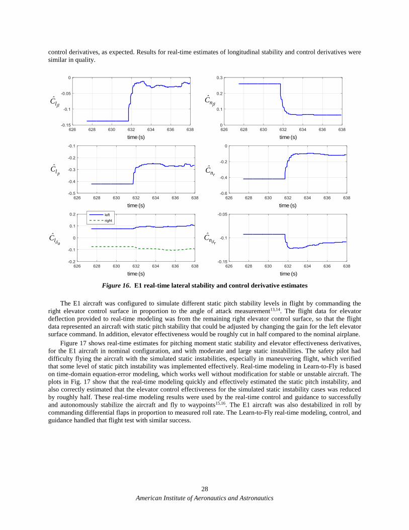
American Institute of Aeronautics and Astronautics
28
control derivatives, as expected. Results for real-time estimates of longitudinal stability and control derivatives were
similar in quality.
Figure 16. E1 real-time lateral stability and control derivative estimates
The E1 aircraft was configured to simulate different static pitch stability levels in flight by commanding the
right elevator control surface in proportion to the angle of attack measurement13,14. The flight data for elevator
deflection provided to real-time modeling was from the remaining right elevator control surface, so that the flight
data represented an aircraft with static pitch stability that could be adjusted by changing the gain for the left elevator
surface command. In addition, elevator effectiveness would be roughly cut in half compared to the nominal airplane.
Figure 17 shows real-time estimates for pitching moment static stability and elevator effectiveness derivatives,
for the E1 aircraft in nominal configuration, and with moderate and large static instabilities. The safety pilot had
difficulty flying the aircraft with the simulated static instabilities, especially in maneuvering flight, which verified
that some level of static pitch instability was implemented effectively. Real-time modeling in Learn-to-Fly is based
on time-domain equation-error modeling, which works well without modification for stable or unstable aircraft. The
plots in Fig. 17 show that the real-time modeling quickly and effectively estimated the static pitch instability, and
also correctly estimated that the elevator control effectiveness for the simulated static instability cases was reduced
by roughly half. These real-time modeling results were used by the real-time control and guidance to successfully
and autonomously stabilize the aircraft and fly to waypoints15,16. The E1 aircraft was also destabilized in roll by
commanding differential flaps in proportion to measured roll rate. The Learn-to-Fly real-time modeling, control, and
guidance handled that flight test with similar success.
nC
plC
rnCa
lC
lC
rnC
time (s)time (s)
time (s)
time (s) time (s)
time (s)

American Institute of Aeronautics and Astronautics
29
Nominal, Flight 6
Moderate Pitch Instability, Flight 9
Large Pitch Instability, Flight 11
Figure 17. Real-time stability and control derivative estimates for nominal stable and destabilized E1
There were two flights of the Woodstock aircraft, each starting from a balloon drop at altitude13,14. On the first
flight, the aircraft was damaged by a collision of the empennage with part of the balloon release structure at the time
of release, and the aircraft was lost.
On the second flight, the aircraft came off the balloon successfully, then recovered using simple and robust rate-
stabilization, attitude-command recovery control to a wings-level descending flight condition at 11.7 deg angle of
attack. The PTI and modeling data collection started on time at 2 seconds into the flight, and operated properly.
Learning adaptive control activated on time at 4 seconds into the flight. Unfortunately, at that time, normal
acceleration was 2.25 g and dynamic pressure was 9.4 lbf/ft2, which were close to the maximum values of those
quantities for the first 30 seconds of the flight. When learning adaptive control activated at 4 seconds, information
from real-time modeling was good, with all main control derivatives showing conventional signs, left and right
aileron effectiveness values matched well in magnitude with opposite and conventional signs as expected, real-time
longitudinal stability derivative estimates showed good static and dynamic pitch stability, and elevator pitch
effectiveness was good with conventional sign. However, both roll and yaw static stability were indicated as
marginally stable, trending toward unstable, as can be seen from the plots on the right side of Fig. 18. Roll damping
plC was stable and relatively steady, but yaw damping rnC was marginally stable, trending toward unstable, as
shown in the lower left plot of Fig. 18. Real-time modeling indicated that nC
was unstable (negative) at 5.1
seconds, and rnC was unstable (positive) at 5.44 seconds, as shown in Fig. 18. After learning adaptive control
activation at 4 seconds, an immediate hard turn to the right was commanded using the ailerons, presumably to head
toward the first waypoint. This happened almost exactly at peak dynamic pressure of 9.84 lbf/ft2. After the turn was
initiated, sideslip angle increased rapidly, peaking at 32.4 deg at 5 seconds into the flight. Real-time modeling
mC e
mC
mC e
mC
mC e
mC
time (s) time (s)
time (s) time (s)
time (s) time (s)

American Institute of Aeronautics and Astronautics
30
indicated that rudder was effective with conventional negative sign, but it appeared that learning adaptive control
was slow to respond to the rapid sideslip angle buildup in the turn. This was followed by an increase in angle of
attack and load factor at high dynamic pressure, and the aircraft appears to stall near 22 deg angle of attack at 5.2
seconds. The stall was followed by a partial recovery and another abrupt increase in angle of attack leading to an
apparent stall at 5.8 seconds that dropped the aircraft out of the turn and into a right spin from which it did not
recover.
In this Learn-to-Fly flight test, the balloon release, recovery control, PTI excitation, and real-time modeling
operated as designed and expected. However, the inherent time lag in real-time modeling results and the rapid
sideslip angle increase from the yaw instability of the novel Woodstock aircraft configuration were not overcome by
the real-time learning adaptive control in time to save the aircraft. Another problem was poor accuracy for flap
effectiveness estimates at high angle of attack and sideslip angle, because the candidate modeling functions used in
real-time modeling did not include nonlinear terms that could account for changes in flap effectiveness with angle of
attack and sideslip angle, although these nonlinear terms were available for the primary controls (ailerons, elevator,
and rudder). Because there were eight wing flaps on the aircraft, checking for nonlinear dependencies on flap
effectiveness required too much computation, and the likelihood of those dependencies was considered low. This led
to the control allocator using the outboard flaps for rolling moment control at a very bad time (high values of
sideslip angle, angle of attack, dynamic pressure, and roll angle, with inaccurate flap effectiveness estimates), which
likely put the aircraft into a spin. The real-time modeling had nonlinear candidate modeling functions capable of
characterizing variations in the effectiveness of the primary controls with angle of attack and sideslip angle, and did
that successfully.
Woodstock Flight 2
Figure 18. Real-time stability and control derivative estimates for Woodstock flight 2
G. Interaction With Other Learn-to-Fly Components
The Learn-to-Fly algorithm required three relatively complex components to operate simultaneously, namely
real-time modeling, real-time learning adaptive control, and real-time guidance. This practical requirement was the
basis for many of the important lessons learned. A list of some of the lessons learned is given in the Conclusions.
This section examines a few of the important interaction effects between real-time modeling and other components
of the Learn-to-Fly algorithm.
rnC
nC
rnC
deg
deg/s
r deg
lC
deg

American Institute of Aeronautics and Astronautics
31
The real-time learning adaptive control used for Learn-to-Fly was based on nonlinear dynamic inversion, which
has a relatively high requirement for model accuracy. But real-time modeling results are stochastic with inherent
time delay and time-varying accuracy that depends on how much data have been collected at any time point, and the
information content in that data. Consequently, the control law has to be not only adaptive and learning, but also has
to adapt the control objectives. These control objectives must be in harmony with the necessarily time-varying
fidelity of the real-time modeling results. For example, in the initial stages of a Learn-to-Fly flight test, the control
law objectives might be simply stabilizing the aircraft at a nominal flight condition, to provide time for the real-time
modeling to get an accurate characterization of the aircraft. With a real-time assessment of the modeling success,
perhaps from prediction error tests, the objectives of the control law could be changed to include improved tracking
accuracy, more precise maneuvering capability, and/or flight envelope expansion. This approach would also help to
alleviate the problems associated with the control law squelching PTI excitations, because initially, when good
modeling data is most important, the control law activity would be subdued and therefore should not impact the PTI
significantly.
A similar interaction effect involves the real-time modeling and the control allocator in the control law. Because
real-time modeling results necessarily have a time-varying and stochastic character, the control allocation should be
simple and robust initially. After the real-time modeling results become more accurate and stable over time, the
control allocator could change to achieve practical objectives that are sensitive to model accuracy, such as
optimizing control allocation for minimum drag.
The real-time guidance component of Learn-to-Fly interacted with real-time modeling by using real-time
estimates of lift/drag ratio as a function of nominal angle of attack, for glide calculations. For the E1 aircraft, the
XC real-time modeling was not valid, as described earlier, so a fixed lift/drag estimate obtained from E1 flight data
with the engine at idle power was used instead of a real-time estimate of lift/drag. This practical work-around was
successful, but using a real-time lift/drag estimate should result in better performance.
Other interactions that were considered, but not implement in Learn-to-Fly, include the use of real-time stability
and control derivative estimates and their trends with time to estimate open-loop stability and control boundaries,
and monitoring data density in explanatory variable space to help real-time guidance direct the nominal flight
condition for effective and efficient flight test envelope expansion.
VI. Conclusions
The traditional approach to flying new or modified aircraft is to conduct a series of ground tests to determine
the aircraft characteristics, then design a control law and flight procedures based on that information. The Learn-to-
Fly approach proposes to design and implement onboard automated algorithms for real-time modeling, real-time
learning adaptive control, and real-time guidance that will reduce or eliminate the need for ground testing, saving
large amounts of time and money, and providing new opportunities for rapid and effective aircraft development and
testing.
The real-time global aerodynamic modeling technique developed for Learn-to-Fly identified global nonlinear
aerodynamic models in real time from flight data alone, and achieved good fits to the modeling data and good
prediction capability for flight data that were not used in the modeling process. Related issues important for the
success of the Learn-to-Fly concept were studied, including onboard implementation, real-time flight data
information content, quality of identified global aerodynamic models as a function of time, speed and accuracy of
the real-time modeling results, accurate real-time stability and control derivative estimates, and integration of multi-
input excitation and real-time global modeling with simultaneous real-time learning adaptive control and real-time
guidance.
The real-time modeling developed and demonstrated for Learn-to-Fly used a time-domain equation-error
modeling approach that combined multivariate orthogonal function modeling based on statistical modeling metrics
with real-time recursive modeling function orthonormalization and the QR decomposition. The method was
successfully applied in flight onboard two subscale aircraft, executing autonomously in real time with reasonable
computational requirements. Accurate global aerodynamic models were identified in real time, based on flight data
alone. The real-time global aerodynamic models exhibited good prediction capability for flight data that were not
used in the modeling process, and developed improved prediction accuracy (learning) over time, as additional
informative data were collected and processed. Furthermore, analytic derivatives of the global models evaluated at
various flight conditions produced good estimates of the aircraft stability and control, indicating that the local
topology of the identified global model was reasonable.

American Institute of Aeronautics and Astronautics
32
Automated orthogonal optimized excitation inputs were applied to all control surfaces simultaneously at
varying flight conditions, resulting in data with rich information content for global nonlinear aerodynamic modeling.
Flight data generated in this way exhibits low correlations among explanatory variables, multi-axis excitation, and
rapid coverage of large portions of the explanatory variable subspace. These characteristics make the inputs very
effective and efficient for real-time global aerodynamic modeling.
The Learn-to-Fly concept was a significant technical stretch, and was intended to be that from the start. Many
important lessons were learned, through both success and failure in attempting to make the Learn-to-Fly concept a
reality. Some of the most important lessons learned were:
1. Real-time modeling results are time-varying and stochastic, because of time-varying data information, noisy
data, and model structure errors. Consequently, real-time control must be robust to model variations with time,
which is not the same as conventional model uncertainty.
2. Real-time modeling and real-time control have opposing objectives, because modeling needs data information
content from dynamic responses, but control is designed to suppress disturbances, among other tasks.
3. Real-time modeling results based on flight data will always have a slight time delay, currently about one cycle
of the dominant dynamic mode frequency, because dependencies must be exhibited in the data before they can
be modeled accurately.
4. More computational capability in the onboard flight computer would enable more accurate global modeling by
allowing larger pools of more diverse candidate modeling functions to be evaluated in real time. The enhanced
pool of candidate modeling functions should include functions with local support, so that modeling a complex
and significant nonlinearity in one region of the explanatory variable space (e.g., at high angle of attack) would
not impact the global model in other regions.
5. For aircraft with thrust acting along the x body axis, the real-time XC nondimensional aerodynamic coefficient
modeling should be changed to real-time XF force modeling with additional candidate modeling functions
included to characterize propulsion effects.
6. Conventional methods for estimating fit error variance from modeling results for model uncertainty
calculations cannot be applied to real-time modeling, because the fit error variance estimates must be available
at interim times, not just at the end of a maneuver.
7. Programmed Test Input (PTI) excitation amplitudes should be selected automatically based on a real-time
estimate of the signal-to-noise ratio of the dependent variables (nondimensional aerodynamic force and
moment coefficients for Learn-to-Fly). The PTI waveforms are designed with wideband frequency content, so
there is no need to change the waveforms. Only the amplitudes need adjustment, which involves changing a
single value for each control surface excitation input.
8. Learn-to-Fly flights should start with 5-10 seconds of wings-level flight at moderate nominal angle of attack
with control surface excitations active, which can be achieved using simple rate-stabilized, attitude-command
feedback control, similar to the recovery mode control developed and used successfully in this work. This
would allow time for baseline learning, after which maneuvering and flight envelope expansion could proceed
using more sophisticated real-time control and guidance. Consequently, Learn-to-Fly requires a relatively large
flight test area.
9. Real-time guidance and control for Learn-to-Fly should adjust objectives from simple stabilization and
nominal wings-level flight at the start to progressively more precise maneuvering and tracking as more
informative data are collected and the real-time models become more accurate and comprehensive. Control law
objectives could adapt to real-time modeling fidelity, quantified by real-time metrics for current modeling
accuracy or approximated as flight time spent in regions of the explanatory variable space with control surface
excitation active.
10. An intelligent executive component is needed in the Learn-to-Fly algorithm, for monitoring and directing the
real-time modeling, control, and guidance so that learning and maneuvering objectives can be accomplished
while avoiding limits related to the flight envelope, control authority, test range, and flight safety.
Addressing these considerations will bring the Learn-to-Fly concept closer to becoming a practical and useful
technique. Learn-to-Fly technology will enable self-learning aircraft, resulting in reduced development cost for new
aircraft, as well as more robust and safe flight operations. The flight testing and modeling techniques described in

American Institute of Aeronautics and Astronautics
33
this work can also be applied to build high-fidelity, full-envelope nonlinear aircraft simulations from flight data, thus
reducing or eliminating the need for extensive wind tunnel testing or aerodynamic calculations.
Acknowledgments
The efforts of the flight test team at NASA Langley Research Center in building and testing the Woodstock and
E1 aircraft and associated systems, carefully calibrating the instrumentation, and carrying out the flight operations to
collect the flight data used in this study, are gratefully acknowledged. This research was funded by the NASA
Aeronautics Research Mission Directorate (ARMD) Convergent Aeronautics Solution (CAS) Learn-to-Fly project.
References 1McNally, B. David, “Full-Envelope Aerodynamic Modeling of the Harrier Aircraft,” NASA TM 88376, October 1986. 2Jategaonkar, R.V., Mönnich, W., Fischenberg, D., and Krag, B. “Identification of C-160 Simulator Data Base from Flight
Data,” Proceedings of the 10th IFAC Symposium on System Identification, Copenhagen, Denmark, Elsevier Sciences Ltd.,
Oxford, UK, 1994, pp. 1031-1038. 3Hui, K., Ricciardi, J., Ellis, K, and Tuomey, D. “Beechjet Flight Test Data Gathering and Level-D Simulator Aerodynamic
Mathematical Model Development,” AIAA 2001-4012, AIAA Atmospheric Flight Mechanics Conference, Montreal, Quebec,
Canada, August 2001. 4Seher-Weiss, S. “Identification of Nonlinear Aerodynamic Derivatives using Classical and Extended Local Model
Networks,” Aerospace Science and Technology, Vol. 15, 2011, pp. 33-44. 5Tobias, E.L., Tischler, M.B., Berger, T., and Hagerott, S.G. “Full Flight-Envelope Simulation and Piloted Fidelity
Assessment of a Business Jet Using a Model Stitching Architecture,” AIAA Modeling and Simulation Technologies Conference,
Kissimmee, FL, January 2015. 6Morelli, E.A. “Real-Time Global Nonlinear Aerodynamic Modeling for Learn-to-Fly,” AIAA-2016-2010, AIAA SciTech
2016 Conference, San Diego, CA, January 2016. 7Morelli, E.A. “Flight Test Maneuver Design for Efficient Aerodynamic Modeling,” AIAA-2011-6672, AIAA Atmospheric
Flight Mechanics Conference, Portland, OR, August 2011. 8Morelli, E.A. “Efficient Global Aerodynamic Modeling from Flight Data,” AIAA-2012-1050, 50th AIAA Aerospace Sciences
Meeting, Nashville, TN, January 2012. 9Brandon, J.M. and Morelli, E.A. “Nonlinear Aerodynamic Modeling From Flight Data Using Advanced Piloted Maneuvers
and Fuzzy Logic,” NASA/TM-2012-217778, October 2012. 10Morelli, E.A., Cunningham, K., and Hill, M.A. “Global Aerodynamic Modeling for Stall/Upset Recovery Training Using
Efficient Piloted Flight Test Techniques,” AIAA 2013-4976, AIAA Modeling and Simulation Technologies Conference,
Boston, MA, August 2013. 11Brandon, J.M. and Morelli, E.A. “Real-Time Global Nonlinear Aerodynamic Modeling from Flight Data,” AIAA-2014-
2554, AIAA Atmospheric Flight Mechanics Conference, Atlanta, GA, June 2014. 12Morelli, E.A. and Klein, V., Aircraft System Identification – Theory and Practice, 2nd Edition, Sunflyte Enterprises,
Williamsburg, VA, 2016. 13Heim, E.H., Viken, E.M., Brandon, J.M., and Croom, M.A. “NASA’s Learn-to-Fly Project Overview,”, AIAA Atmospheric
Flight Mechanics Conference, AIAA Aviation Forum, Atlanta, GA, June 2018, to be published. 14Riddick, S. E., Busan, R. C., Cox, D. E., and Laughter, S. A., “Learn-to-Fly Test Setup and Concept of Operations,”,
Atmospheric Flight Mechanics Conference, AIAA Aviation Forum, Atlanta, GA, June, 2018, to be published. 15Snyder, S. M., Bacon, B. J., Morelli, E. A., Frost, S., Teubert, C., and Okolo, W. “Online Control Design for Learn-to-Fly,”
Atmospheric Flight Mechanics Conference, AIAA Aviation Forum, Atlanta, GA, June, 2018, to be published. 16Foster, J. V., “Autonomous Guidance Algorithms for NASA Learn-to-Fly Technology Development,” Atmospheric Flight
Mechanics Conference, AIAA Aviation Forum, Atlanta, GA, June, 2018, to be published. 17Morelli, E.A. “Global Nonlinear Aerodynamic Modeling using Multivariate Orthogonal Functions,” Journal of Aircraft,
Vol. 32, No. 2, March-April 1995, pp. 270-77. 18Gentleman, W.M. “Least Squares Computation by Givens Transformation Without Square Roots,” Journal of the Institute
for Mathematics Applications, Vol. 12, 1973, pp. 329-336. 19Gentleman, W.M. “Regression Problems and the QR Decomposition,” Bulletin of the Institute for Mathematics
Applications, Vol. 10, 1974, pp. 195-197. 20https://software.nasa.gov/software/LAR-16100-1 21Morelli, E.A. “Flight-Test Experiment Design for Characterizing Stability and Control of Hypersonic Vehicles,” Journal of
Guidance, Control, and Dynamics, Vol. 32, No. 3, May-June 2009, pp. 949-959. 22Morelli, E.A. and Smith, M.S. “Real-Time Dynamic Modeling – Data Information Requirements and Flight Test Results,”
Journal of Aircraft, Vol. 46, No. 6, November-December 2009, pp. 1894-1905.

American Institute of Aeronautics and Astronautics
34
23Press, W.H., S.A. Teukolsky, W.T. Vettering, and B.R. Flannery Numerical Recipes in FORTRAN: The Art of Scientific
Computing, 2nd Ed., Cambridge University Press, New York, NY, 1992. 24Morelli, E.A., “Practical Aspects of the Equation-Error Method for Aircraft Parameter Estimation,” AIAA-2006-6144,
AIAA Atmospheric Flight Mechanics Conference, Keystone, CO, August 2006. 25Barron, A.R., “Predicted Squared Error : A Criterion for Automatic Model Selection,” Self-Organizing Methods in
Modeling, Farlow, S.J., Ed., Marcel Dekker, Inc., New York, NY, 1984, pp. 87-104. 26Grauer, J.A. and Morelli, E.A. “Method for Real-Time Frequency Response and Uncertainty Estimation,” Journal of
Guidance, Control, and Dynamics, Vol. 37, No. 1, January-February 2014, pp. 336-343. 27Grauer, J.A. and Morelli, E.A. “A Generic Global Aerodynamic Model for Aircraft,” Journal of Aircraft, Vol. 52, No. 1,
January-February 2015, pp. 13-20.
Table 1. Aircraft geometry and mass properties
Woodstock E1
c , ft 1.671 1.966
b , ft 7.600 10.167
S , ft2 6.944 19.264
cgx , in -1.750 -3.022
cgy , in 0.000 0.000
cgz , in 0.063 0.000
refx , in -1.750 -3.012
refy , in 0.000 0.000
refz , in 0.000 0.000
m , slugs 0.881 1.856
xI , slugs-ft2 0.797 2.639
yI , slugs-ft2 0.965 6.081
zI , slugs-ft2 1.811 8.166
xzI , slugs-ft2 0.000 0.000
Table 2. E1 Elevator Programmed Test Input (PTI) Design
Input T (s) A (deg) k kA (deg) k (rad) RPF
e 0.866 2.2272
0.866 1.1783
0.866 2.2747
0.866 2.1205
0.866 1.5285
0.866 2.8381
0.866 2.8768
0.866 3.1406
0.866 0.2472
0.866 2.4717
0.866 0.2847
0.866

American Institute of Aeronautics and Astronautics
35
Table 3. E1 Research Flight Data
Flight
Number Flight Description
1 Pilot familiarity, pitch-yaw-roll doublets, PTI checkout, real-time modeling checkout
2
PTI checkout, pitch-yaw-roll doublets, PTI in approaches to stall, real-time modeling
checkout, successful real-time modeling, learning adaptive control, and guidance to
waypoints
3 PTI checkout, pitch-yaw-roll doublets, successful real-time modeling, learning adaptive
control with disturbance rejection, and guidance to waypoints
4
PTI checkout, pitch-yaw-roll doublets, successful real-time modeling from various entry
conditions, GP learning control had mixed results dependent on entry conditions, mostly
successful longitudinally but exhibited increasing roll oscillations at high speed, practiced
unusual attitude entry conditions to emulate Woodstock balloon drop conditions
5
Learn-to-Fly flight test emulation starting from emulated balloon drop conditions,
allowing 4 s delay for PTI and real-time modeling, then invoking learning adaptive control
and guidance, successful real-time modeling, learning adaptive control, and guidance to
waypoints
6
Real-time modeling timing tests, starting from level flight, allowing 4 s, 2 s, and 0 s for
PTI and real-time modeling, then invoking learning adaptive control and guidance,
successful real-time modeling and learning adaptive control for all cases, guidance had
mixed success, sometimes navigating to wrong waypoints
7
Learn-to-Fly flight test emulation starting from emulated balloon drop conditions,
allowing 2 s for PTI and real-time modeling, then invoking learning adaptive control and
guidance, mixed results dependent on entry conditions, relatively high winds
8
Learn-to-Fly flight test emulation starting from a variety of emulated balloon drop
conditions, allowing 1 s delay for recovery, 1 s for PTI and real-time modeling, then
invoking learning adaptive control and guidance, modified based on initial Woodstock
flight test data, most successful, but mixed results dependent on entry conditions
9
Artificial longitudinal destabilization to -10% static margin using angle of attack feedback
to left elevator, two entries, both with successful real-time modeling, learning adaptive
control, and guidance to waypoints
10
Artificial lateral destabilization to 0.1 s time to double in roll using roll rate feedback to
differential flaps, two entries, both with successful real-time modeling, learning adaptive
control, and guidance to waypoints
11
Artificial longitudinal destabilization to -20% static margin using angle of attack feedback
to left elevator, two entries, both with successful real-time modeling, learning adaptive
control, and guidance to waypoints
Table 4. Woodstock Research Flight Data
Flight
Number Flight Description and Objective
1 Learn-to-Fly flight test, structural failure from vertical tail impacting a support upon
release from the balloon
2 Learn-to-Fly flight test, unrecovered spin departure in the first turn toward the first
waypoint due to control mode switch failure