Ecological Modelling, 42 (1988) 265-287

Elsevier Science Publishers B.V., Amsterdam - Printed in The Netherlands 265

PRACTICAL ASPECTS OF MODELLING ECOLOGICAL PHENOMENA USING THE CUSP CATASTROPHE

CHANTAL OUIMET and PIERRE LEGENDRE

DCpartement de Sciences biologiques, Universitk de Mont&al, C.P. 6128, Succ. A, Mont&al,

Que. H3C 3J7 (Canada)

(Accepted 10 February 1988)

ABSTRACT

Ouimet, C. and Legendre, P., 1988. Practical aspects of modelling ecological phenomena using the cusp catastrophe. Ecol. Modelling, 42: 265-287.

Understanding discontinuities helps to better comprehend biological systems. Catastrophe theory deals with discontinuities and provides a way of modelling them, but the mathematical steps used to do so are often out of reach for many biologists. To solve this problem, graphs and nonlinear regression steps are proposed for the cusp catastrophe. A special F statistic is used to test if the cusp model fits the data better than a plane model would. Made-up data are used to demonstrate how to use the proposed procedure. The last part of the paper is concerned with the design of sampling programs adapted to cusp catastrophe modelling; a two-step procedure is recommended, when feasible. An Appendix contains a short reminder on catastrophe theory, with emphasis on the cusp catastrophe.

1. INTRODUCTION

Modelling, in biology and ecology, serves two main purposes. First, a model can be used to synthesize the information collected about a system, in order to verify its coherence and completeness. Second, confirming the predictions derived from a model shows that the data support the hypothe- ses built into the model, which gives us new insights into the processes controlling the system under study and makes it possible to use these predictions for management purpose. In this way, modelling enhances our understanding of ecological systems.

In spite of the many types of mathematics that are currently used in modelling, many phenomena cannot be properly modelled. This is the case for example for those natural phenomena in which one finds discontinuities that cannot be explained by any obvious trigger. This type of discontinuity can be dealt with using a mathematical theory stated in 1972 by RenC Thorn,

0304-3800/88/$03.50 0 1988 Elsevier Science Publishers B.V.

266

which is called catastrophe theory. The first application of this theory was in the modelling of morphogenesis in embryology (Thorn, 1972, 1975). It has been widely used in physics (Gilmore, 1981; Poston and Stewart, 1978) and in chemistry to describe, from a new angle, such well-known phenomena as the caustic effects in light, rainbows, earthquakes, etc. In biology, and especially in ecology, progress has been slower, and today only a small number of models use catastrophe theory.

Two major factors explain the slow evolution of this theory in biology: (1) catastrophe theory is based on a highly specialised mathematic field, topol- ogy; and (2) the steps to follow in order to build a catastrophe model are seldom explained in layman’s terms, outside the specialized mathematical literature.

Nevertheless, catastrophe theory could open the door to a better under- standing of several ecological phenomena. To do this, the theory uses eleven elementary catastrophe shapes, of which the cusp is the most widely used. The cusp is often the choice of authors to model phenomena that include continuous and discontinuous behaviors, because it is the one catastrophe shape that associates a discontinuous response with two control variables. This is about as complex an interaction as modellers are usually willing to tackle, and it can still be easily represented graphically. Higher levels of interaction are more difficult to grasp, and also to communicate to other researchers.

To take advantage of these properties without having to rely upon complex mathematics, graphical and non-linear regression steps are sug- gested in this paper for building a cusp catastrophe model. An Appendix presents a reminder of the basics of catastrophe theory and of the cusp catastrophe model.

2. HOW TO SPOT SIGNS OF A CATASTROPHE IN DATA

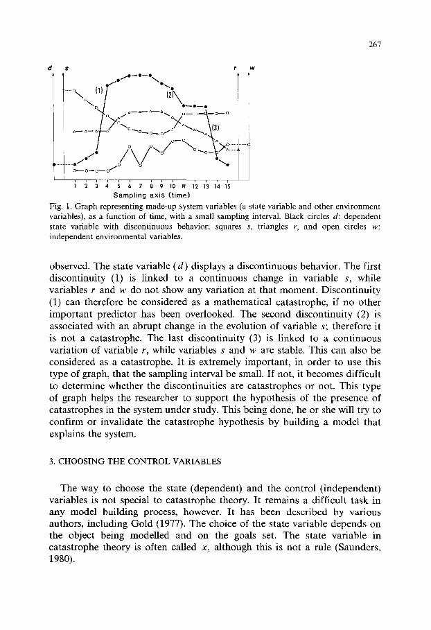
The first step to complete before launching a catastrophe modelling project is to determine whether a catastrophe is present or not. This can be done from data obtained by sampling the environment, or on theoretical grounds alone. Based on some a priori knowledge of the system, one can hypothesize that catastrophes are present in the system’s behavior and prepare to collect data to demonstrate this. Section 7 explains some im- portant principles to follow when sampling with catastrophe theory in mind. When the data have been collected, this first step (looking for catastrophes) can be carried out by examining graphs of different system variables as a function of time, or space, or any other axis used for sampling. This type of graph allows one to find out if the discontinuities observed in the data are mathematical catastrophes or not. Figure 1 is an example of what might be

267

d s I w

12 3 4 5 6 7 8 9 10 11 12 13 14 15

Sampling axis (time)

Fig. 1. Graph representing made-up system variables (a state variable and other environment variables), as a function of time, with a small sampling interval. Black circles d: dependent state variable with discontinuous behavior; squares s, triangles r, and open circles w: independent environmental variables.

observed. The state variable (d) displays a discontinuous behavior. The first discontinuity (1) is linked to a continuous change in variable s, while variables Y and w do not show any variation at that moment. Discontinuity (1) can therefore be considered as a mathematical catastrophe, if no other important predictor has been overlooked. The second discontinuity (2) is associated with an abrupt change in the evolution of variable s; therefore it is not a catastrophe. The last discontinuity (3) is linked to a continuous variation of variable r, while variables s and w are stable. This can also be considered as a catastrophe. It is extremely important, in order to use this type of graph, that the sampling interval be small. If not, it becomes difficult to determine whether the discontinuities are catastrophes or not. This type of graph helps the researcher to support the hypothesis of the presence of catastrophes in the system under study. This being done, he or she will try to confirm or invalidate the catastrophe hypothesis by building a model that explains the system.

3. CHOOSING THE CONTROL VARIABLES

The way to choose the state (dependent) and the control (independent) variables is not special to catastrophe theory. It remains a difficult task in any model building process, however. It has been described by various authors, including Gold (1977). The choice of the state variable depends on the object being modelled and on the goals set. The state variable in catastrophe theory is often called x, although this is not a rule (Saunders, 1980).

As for the control variables, the choice can be made in many different ways. In some cases, it can be based on a specific theory that requires only testing. Alternatively, data analysis (clustering, ordinations, regression, non- linear path analysis, etc.) can provide clues as to the causal interactions among variables; these clues can in turn become a theory after controlled experiments in the lab or in nature. A data analysis method as simple as plotting the graph in Fig. 1 can also help choose the variables that are responsible for the catastrophes. A judicious choice of the control variables is essential. If an important variable has been left out and it is one that varies abruptly, then what was thought to be a catastrophe is not one. On the other hand, if an important variable responsible for the catastrophes is left out, then the model should probably pertain to a more complicated catastrophe type. In both cases, the model will be incomplete and even false. The choice of the control variables has to be made with caution, with full knowledge of the pitfalls involved.

For the cusp catastrophe, the required number of control variables is two. These two variables can be read directly from the data set, or they can result from combining several variables, for instance by regression or by some form of factor analysis (ordination). This procedure is frequently used; then the number of variables involved does not matter, since in the end only two axes are obtained to form the control surface. The control variables u and u are thus functions of the different variables measured in the system. Exam- ples of such data reduction are found in Harmsen et al. (1976), Kempf (1980) and Rose and Harmsen (1981). Sections and projections of data (graphs) will help choose the system variables needed for building the model. Here we will use d, Y and s as the names of the actual variables. The names X, u and u are generally reserved to represent the theoretical variables of the cusp. When one works with real data, one does not know from the start if Y = u and s = u, or conversely, if r = u and s = u. Until this is known, it is better to use different names for the theoretical variables and the data variables.

The graph of d (the state variable) as a function of s (a control variable), with r (the other control variable) constant, represents a section through the cusp. If s = u (in other words, if s is the normal factor), this graph has an ‘S-shape, or a more or less well-defined mirror image of an ‘S’ (Fig. 2). With real data, the central part (dashed line in Fig. 2) should not show up in sections of the cusp where r < 0 (if r is the splitting factor), because we are then in the area of the cusp fold, and in this area the dashed line (central sheet) corresponds to an improbable behavior. This graph makes it possible to spot the chief properties of the cusp, namely discontinuity, bimodality, hysteresis and inaccessibility. Only the divergence property cannot be evi- denced by this type of graph.

269

I I s I

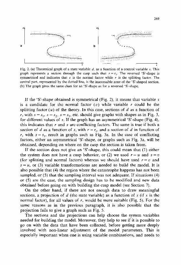
Fig. 2. (a) Theoretical graph of a state variable d, as a function of a control variable S. This graph represents a section through the cusp such that r = rl. The reversed ‘S’-shape is symmetrical and indicates that s is the normal factor while r is the splitting factor. The central part, represented by the dotted line, is the inaccessible zone of the ‘S-shaped section.

(b) The graph gives the same clues for an ‘S-shape as for a reversed ‘S-shape.

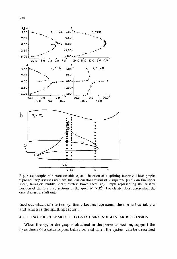
If the ‘S-shape obtained is symmetrical (Fig. 2) it means that variable s is a candidate for the normal factor (u) while variable r could be the splitting factor (u) of the theory. In this case, sections of d as a function of r, with s = sr, s = s2, s = sj, etc. should give graphs with shapes as in Fig. 3, for different values of s. If the graph has an asymmetrical ‘S-shape (Fig. 4), this indicates that r and s are conflicting factors. The same is true if both a section of d as a function of s, with Y = rr, and a section of d in function of r, with s = sr, result in graphs such as Fig. 3a. In the case of conflicting factors, either an asymmetrical ‘S-shape, or graphs such as Fig. 3a, will be obtained, depending on where on the cusp the section is taken from.

If the section does not give an ‘S-shape, this could mean that (1) either the system does not have a cusp behavior, or (2) we used r = u and s = u (for splitting and normal factors) whereas we should have used r = u and s = U, or (3) variable transformations are needed to build the model. It is also possible that (4) the region where the catastrophe happens has not been sampled, or (5) that the sampling interval was not adequate. If situations (4) or (5) are the case, the sampling design has to be modified and new data obtained before going on with building the cusp model (see Section 7).

On the other hand, if there are not enough data to draw meaningful sections, a projection of d (the state variable) as a function of s (if s is the normal factor), for all values of r, would be more suitable (Fig. 5). For the same reasons as in the previous paragraph, it is also possible that the projection fails to give a graph such as Fig. 5.

The sections and the projections can help choose the system variables needed for building the model. Moreover, they help to see if it is possible to go on with the data that have been collected, before getting more deeply involved with non-linear adjustment of the model parameters. This is especially important when one is using variable combinations, and needs to

270

-24,0-1&O -12,0 -6,0 0,O ’

_:-_::.,~~~...~i:-_

-24,0 -9,0 9,0 ’ -90,o -45,o ’

90,o ’ -15.0 0,o 15,0 45,o

b

$ . . . - . . . \

. ‘.ii =

.

.

-0,5 .

0 1,5 10 s

Fig. 3. (a) Graphs of a state variable d, as a function of a splitting factor r. These graphs represent cusp sections obtained for four constant values of s. Squares: points on the upper sheet; triangles: middle sheet; circles: lower sheet. (b) Graph representing the relative position of the four cusp sections in the space R, X Rf,. For clarity, dots representing the central sheet are left out.

find out which of the two synthetic factors represents the normal variable u and which is the splitting factor U.

4. FITTING THE CUSP MODEL TO DATA USING NON-LINEAR REGRESSION

When theory, or the graphs obtained in the previous section, support the hypothesis of a catastrophic behavior, and when the system can be described

271

d*

----‘;I ;: ,/ ,/’

,___......_...... -.- cl___ I .

s

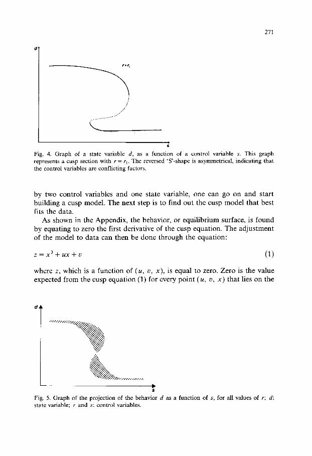
Fig. 4. Graph of a state variable d, as a function of a control variable S. This graph represents a cusp section with r = rl. The reversed ‘S-shape is asymmetrical, indicating that the control variables are conflicting factors.

by two control variables and one state variable, one can go on and start building a cusp model. The next step is to find out the cusp model that best fits the data.

As shown in the Appendix, the behavior, or equilibrium surface, is found by equating to zero the first derivative of the cusp equation. The adjustment of the model to data can then be done through the equation:

z=x3+ux+u (1)

where z, which is a function of (u, u, x), is equal to zero. Zero is the value expected from the cusp equation (1) for every point (u, u, x) that lies on the

d

Fig. 5. Graph of the projection of the behavior d as a function of s, for all values of r; d:

state variable; r and S: control variables.

272

x t

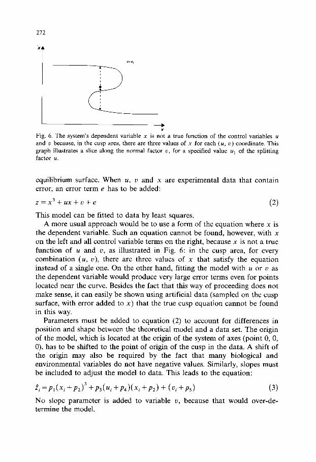
Fig. 6. The system’s dependent variable x is not a true function of the control variables u and u because, in the cusp area, there are three values of x for each (u, u) coordinate. This graph illustrates a slice along the normal factor u, for a specified value u1 of the splitting factor u.

equilibrium surface. When U, u and x are experimental data that contain error, an error term e has to be added:

z=x3+z4x+u+e

This model can be fitted to data by least squares.

(2)

A more usual approach would be to use a form of the equation where x is the dependent variable. Such an equation cannot be found, however, with x on the left and all control variable terms on the right, because x is not a true function of u and u, as illustrated in Fig. 6: in the cusp area, for every combination (u, u), there are three values of x that satisfy the equation instead of a single one. On the other hand, fitting the model with u or u as the dependent variable would produce very large error terms even for points located near the curve. Besides the fact that this way of proceeding does not make sense, it can easily be shown using artificial data (sampled on the cusp surface, with error added to x) that the true cusp equation cannot be found in this way.

Parameters must be added to equation (2) to account for differences in position and shape between the theoretical model and a data set. The origin of the model, which is located at the origin of the system of axes (point 0, 0, 0), has to be shifted to the point of origin of the cusp in the data. A shift of the origin may also be required by the fact that many biological and environmental variables do not have negative values. Similarly, slopes must be included to adjust the model to data. This leads to the equation:

ii=P1(x~ +P2)3 +P3C”i +P4)txi +P*) + C”i +PS) (3)

No slope parameter is added to variable u, because that would over-de- termine the model.

273

The ii’s are the values of variable z as estimated by the model. As in ordinary regression, the residuals are computed as (z, - ;,), which is ( - 5,) in the present case since all z,‘s are zero. The fitting of the model’s parameters of equation (3) is accomplished by nonlinear regression using least-squares. Several standard statistical packages contain nonlinear regres- sion subprograms that can be used for this purpose, including BMDP (subprogram BMDPAR), SAS (subprogram NLIN) and SPSS (subprogram NONLINEAR). Subprogram ZXSSQ, from the IMSL subroutine library, can also be called from one’s own program for least-squares nonlinear adjustment (Levenberg-Marquardt algorithm).

Testing the adjustment of equation (3) to data is not a simple matter. Because the z, are a vector of zeroes, then the total sum of squares of the dependent variable is zero, so that the coefficient of determination R2 is undetermined and the usual F statistic cannot be computed. According to Kempf (1980), the lack of an appropriate method for testing the degree of adjustment of a cusp model to data is the chief reason why the use of catastrophe theory has progressed so slowly in biology. As an alternative, Legendre et al. (submitted) have proposed to test whether a cusp model fits the data significantly better than a plane model, also adjusted to the data by a nonlinear regression subprogram. They have shown that the plane with equation:

i; = qlxi + q2u; + u, + q3 (4)

is a model nested in the cusp model of equation (3) with z again a vector of zeroes, so that the residual sum of squares (SS Residual) of these two models can be used to build a test of significance. An F statistic is constructed, where the numerator and the denominator represent two independent mean squares:

F = (SS Residual plane - SS Residual cusp)/2

SS Residual cusp/( n - 5) (5)

Of course, the same data set (u, u, x) has to be used to fit equations (3) and (4). Legendre et al. (submitted) have demonstrated, using Monte Carlo simulations, that this test statistic is distributed like an F at least in the part of the F distribution used for testing. They have shown further that this procedure is able to detect a cusp even when the data contain a reasonable amount of error. This presupposes, of course, that the cusp region has been sampled intensively enough, which is the subject of the present paper.

5. HOW TO LOCATE THE BIFURCATION SET

When the F test indicates that the cusp model fits the data better than the plane model does, one can proceed to locating the bifurcation set on the

274

control surface. To do so, we follow the same steps as those used to derive the theoretical bifurcation set equation (A4 in the Appendix): starting from equation (3) that contains the slope and shift parameters p1 to pS, we find the equation of the points that satisfy both equation (3) and its derivative. This equation is:

It is especially interesting to locate the bifurcation set when analyzing data from a preliminary sampling program. To draw the bifurcation set, we choose values of variable u (supposing here that Y = u is the splitting factor) and calculate, using equation (6), the corresponding values of variable u. In this way we get the set of points (u, U) that delimit the cusp and will enable us to design a sampling program with variable pace (Section 7). This new sampling program will be focused on the cusp catastrophe area and thus will make it possible to build a more precise cusp model, as given by equation

TABLE 1

Summary of the steps involved in developing a cusp catastrophe model, using graphs and nonlinear regressions

I To spot signs of catastrophes: Check the presence of the different properties, at least intuitively.

II (A) Choosing the state variable: It depends on the objective of the study. (B) Choosing the control variables:

_ intuitive method (for qualitative models); _ graphs representing the state and the potential control variable as a function of

time (or space); - graphs of the state variable as a function of the control variables; look for an

‘S-shape in sections and in projections; _ create synthetic control variables by regression, ordination, etc.; _ literature; _ controlled environment experiments.

III Cusp catastrophe model: (A) To find the best-fitting cusp equation: Nonlinear regression, using a vector of zeroes

as the dependent variable. (B) To test the fit of the cusp model to data: F test of the difference between the

residuals of the adjustment to a cusp and to a plane model. (C) To localize the bifurcation set (the set of points where the catastrophe occurs): Put

the parameters obtained by nonlinear regression into the equation of the bifurcation set (equation 6).

IV Design a variable-pace sampling program, based upon the position of the bifurcation set in the control variables’ space.

275

(3). It is important to notice that equation (3) represents a cusp only if the F test indicates that the cusp model fits the data better than the plane model does, in which case it is possible to draw the bifurcation set when using the parameters obtained in equation (3). Table 1 summarizes the building steps of a cusp catastrophe model.

6. USE OF THE CUSP MODEL BUILDING STEPS: MADE-UP EXAMPLE

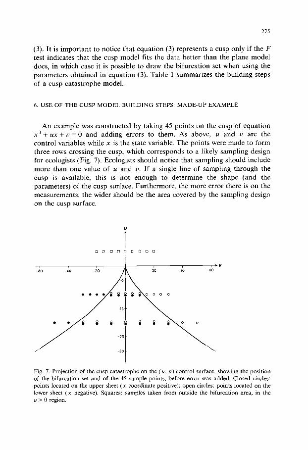
An example was constructed by taking 45 points on the cusp of equation x3 + ux + u = 0 and adding errors to them. As above, u and u are the control variables while x is the state variable. The points were made to form three rows crossing the cusp, which corresponds to a likely sampling design for ecologists (Fig. 7). Ecologists should notice that sampling should include more than one value of u and u. If a single line of sampling through the cusp is available, this is not enough to determine the shape (and the parameters) of the cusp surface. Furthermore, the more error there is on the measurements, the wider should be the area covered by the sampling design on the cusp surface.

I I 1 I .v

-60 -40 -20 20 40 60

Fig. 7. Projection of the cusp catastrophe on the (u, u) control surface, showing the position of the bifurcation set and of the 45 sample points, before error was added. Closed circles: points located on the upper sheet (x coordinate positive); open circles: points located on the lower sheet (x negative). Squares: samples taken from outside the bifurcation area, in the u > 0 region.

276

In this example, nine points were taken at regular intervals on a line of equation u = 5, with a spacing of 5 along the u axis. Eighteen points were placed on a line of equation u = - 10, at regular intervals of 5 along u; half of them are located on the upper sheet of the cusp, while the other half are on the lower sheet. Finally, 18 points were positioned on a line of equation u = - 20, at regular intervals of 10 along u; half of them are on the upper sheet while the other half are on the lower sheet. No point was positioned on the middle sheet of the cusp, since this sheet exerts a repulsive action on points. Error terms were produced using the random normal deviate genera- tor subroutine GGNML of IMSL, and were added to the point coordinates. Since the range of variation on x is not the same as that on u or on u, the random normal deviates, drawn from a (0, 1) normal distribution, were multiplied by a different factor on each axis, in such a way as to get a mean error percentage of 10% on each axis. The mean error percentage, for each of the three variables, was computed as the ratio of the standard deviation of the error terms over the standard deviation of the data values.

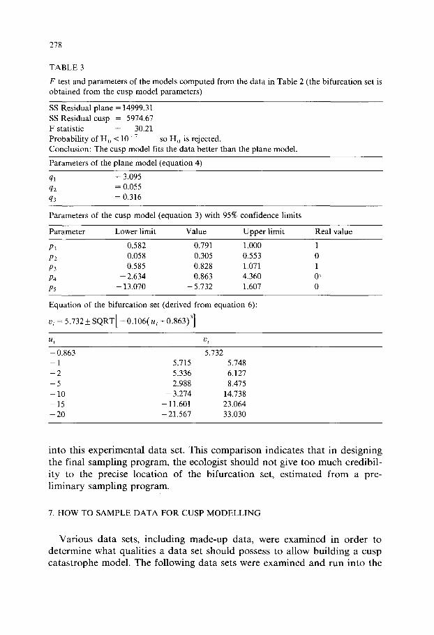
The resulting data set is shown in Table 2. A cusp and a plane model were then fitted to the data set. The results are summarized in Table 3. The F test was performed; it shows that the cusp model fits the data better than the plane model, with a probability of a Type I error less than lo-‘. The Table also shows the confidence intervals, computed for the parameters of the cusp model under a linear hypothesis. In the present case, this hypothesis cannot be sustained, of course, so that the confidence limits in Table 3 must only be taken as general indications of the variability to be expected from the estimations of the parameters. Table 3 shows for instance that the confi- dence interval of parameter p2 is too small to include the true value of the parameter. Sampling a section of the cusp at random would probably have made the parameter estimations more accurate, but this an unlikely sam- pling design in environmental research.

Using the parameters of the cusp model, the bifurcation set can be located. The bifurcation set equation (6) uses four of the five parameters of the cusp model, excluding parameter pz that happens to have poorly estimated confidence intervals, under the linearity assumption. The bifurca- tion set drawn from the cusp model’s parameters is compared in Fig. 8 to the true bifurcation set. Examination of the regression residuals ( - .?) along the three transects of Fig. 7 shows that the small jumps that can be observed in the residual values, near some of the points located in the zone where the cusp has been displaced (Fig. S), are within the bounds of the 45 observed residual values. This shows that the difference in the position of the bifurcation set is not due to the inadequacy of the nonlinear adjustment algorithm under conditions of non-random sampling, as it might have been the case, but can rather be attributed mostly to the sampling variance built

277

TABLE 2

The file with 45 points from Fig. 7, with 10% error added to the u, x and u coordinates

IA X 0 Z

6.675592 0.069047 0.216745 0.000000

4.412278

5.666038

5.160128

5.929957

3.438756

7.045749

5.235439

6.156060

- 10.277966

- 11.966138

- 9.798377

- 10.025887

- 10.878095

- 10.729467

- 10.782113

- 11.231788

- 10.244176

- 10.363140

- 10.981610

- 9.847771

- 8.831753

- 10.508881

- 8.833925

- 10.690011

- 11.543621

- 9.494024

- 18.952929

- 21.690231

- 18.889130

- 20.048804

- 19.562582

- 19.623815

- 19.138062

- 20.089234

- 19.185577

- 19.622723

- 20.876951

- 19.994242

- 19.728940

- 19.572049

- 19.490899

- 20.034247

- 21.496164

- 19.934037

- 0.665831

- 1.608770

- 1.240045

- 2.689791

0.514055

1.272006

2.280291

1.792980

- 3.893300

- 4.047400

- 3.219292

- 3.177638

-4.003813

- 3.842118

- 2.925062

- 2.468307

- 2.069975

2.779532

3.258609

3.555880

3.306615

3.675153

3.361446

4.225045

4.309017

3.547719

- 5.244735

- 5.585720

- 5.757461

- 5.366251

- 4.647199

- 4.732469

- 4.410649

- 4.210497

- 2.963763

3.054155

4.534955

4.308537

4.168885

4.735378

4.411576

4.792579

4.755330

5.375917

5.411711

8.768940

13.399772

17.298943

- 5.864243

- 11.376716

- 15.642767

- 22.672084

29.276534

28.442475

20.937932

14.243360

11.919988

6.925697

1.675152

- 4.493400

- 8.713510

10.352864

7.385852

4.204575

- 1.135777

- 11.479670

- 13.271600

- 24.431465

- 24.117344

- 30.413275

51.050338

43.212091

27.918216

19.591977

11.867846

- 1.081610

- 10.438325

- 23.171450

- 31.893922

34.847526

20.869703

12.298238

- 0.030311

- 11.587393

- 21.912514

- 27.112535

- 35.947163

- 50.000696

0.000000 0.000000

0.000000

0.000000 0.000000 0.000000 0.000000

0.000000 0.000000

0.000000 0.000000 0.000000 0.000000 0.000000 0.000000 0.000000 0.000000 0.000000 0.000000 0.000000 0.000000 0.000000 0.000000

0.000000 0.000000 0.000000 0.000000 0.000000 0.000000 0.000000 0.000000 0.000000 0.000000

0.000000

0.000000

0.000000

0.000000

0.000000 0.000000 0.000000

0.000000 0.000000 0.000000

0.000000

278

TABLE 3

F test and parameters of the models computed from the data in Table 2 (the bifurcation set is obtained from the cusp model parameters)

SS Residual plane = 14999.31

SS Residual cusp = 5974.67 F statistic = 30.21 Probability of H, < 1O-7 so H, is rejected. Conclusion: The cusp model fits the data better than the plane model.

Parameters of the plane model (equation 4)

41 = 3.095

42 = 0.055

q3 = 0.316

Parameters of the cusp model (equation 3) with 95% confidence limits

Parameter Lower limit Value Upper limit Real value

PI 0.582 0.791 1.000 1 P2 0.058 0.305 0.553 0 P3 0.585 0.828 1.071 1 P4 - 2.634 0.863 4.360 0; PS - 13.070 - 5.732 1.607 0

Equation of the bifurcation set (derived from equation 6):

u, = 5.732iSQRT[ -O.l06(u, +0.863)3]

- 0.863 5.732 -1 5.715 5.748 -2 5.336 6.127 -5 2.988 8.475 -10 - 3.274 14.738 -15 - 11.601 23.064 -20 - 21.567 33.030

into this experimental data set. This comparison indicates that in designing the final sampling program, the ecologist should not give too much credibil- ity to the precise location of the bifurcation set, estimated from a pre- liminary sampling program.

7. HOW TO SAMPLE DATA FOR CUSP MODELLING

Various data sets, including made-up data, were examined in order to determine what qualities a data set should possess to allow building a cusp catastrophe model. The following data sets were examined and run into the

279

ll

IO i

.V I

-30

_...-* ,...--

/...~‘- _.....

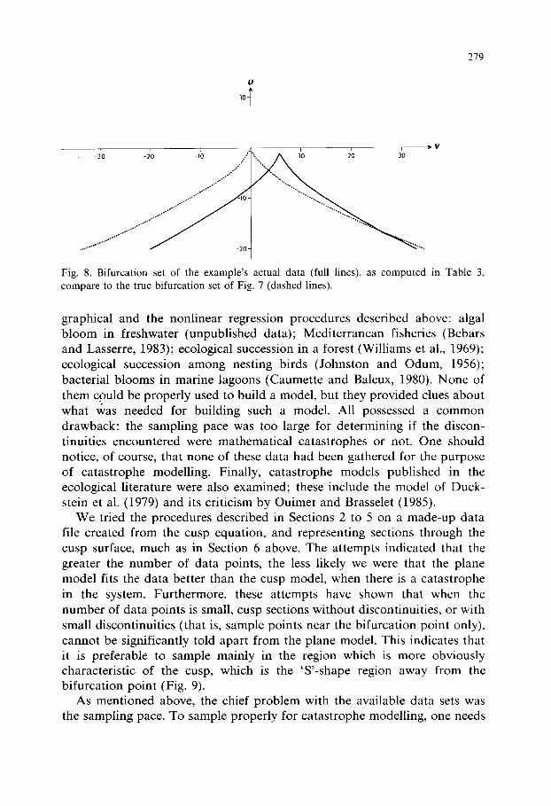
Fig. 8. Bifurcation set of the example’s actual data (full lines), as computed in Table 3, compare to the true bifurcation set of Fig. 7 (dashed lines).

graphical and the nonlinear regression procedures described above: algal bloom in freshwater (unpublished data); Mediterranean fisheries (Bebars and Lasserre, 1983); ecological succession in a forest (Williams et al., 1969); ecological succession among nesting birds (Johnston and Odum, 1956); bacterial blooms in marine lagoons (Caumette and Baleux, 1980). None of them could be properly used to build a model, but they provided clues about what was needed for building such a model. All possessed a common drawback: the sampling pace was too large for determining if the discon- tinuities encountered were mathematical catastrophes or not. One should notice, of course, that none of these data had been gathered for the purpose of catastrophe modelling. Finally, catastrophe models published in the ecological literature were also examined; these include the model of Duck- stein et al. (1979) and its criticism by Ouimet and Brasselet (1985).

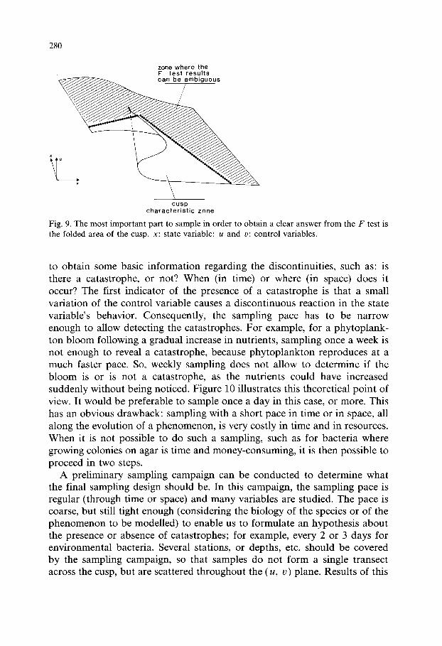
We tried the procedures described in Sections 2 to 5 on a made-up data file created from the cusp equation, and representing sections through the cusp surface, much as in Section 6 above. The attempts indicated that the greater the number of data points, the less likely we were that the plane model fits the data better than the cusp model, when there is a catastrophe in the system. Furthermore, these attempts have shown that when the number of data points is small, cusp sections without discontinuities, or with small discontinuities (that is, sample points near the bifurcation point only), cannot be significantly told apart from the plane model. This indicates that it is preferable to sample mainly in the region which is more obviously characteristic of the cusp, which is the ‘S-shape region away from the bifurcation point (Fig. 9).

As mentioned above, the chief problem with the available data sets was the sampling pace. To sample properly for catastrophe modelling, one needs

280

zone where the F- test results

\ CUSp

characteristic zone

Fig. 9. The most important part to sample in order to obtain a clear answer from the F test is the folded area of the cusp. x: state variable; u and u: control variables.

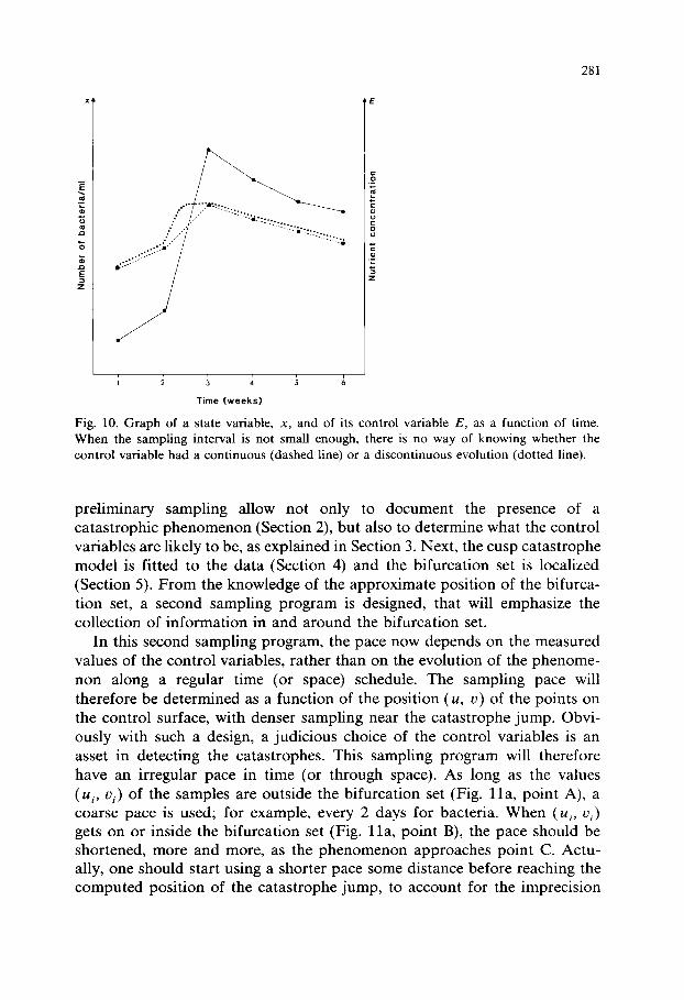
to obtain some basic information regarding the discontinuities, such as: is there a catastrophe, or not? When (in time) or where (in space) does it occur? The first indicator of the presence of a catastrophe is that a small variation of the control variable causes a discontinuous reaction in the state variable’s behavior. Consequently, the sampling pace has to be narrow enough to allow detecting the catastrophes. For example, for a phytoplank- ton bloom following a gradual increase in nutrients, sampling once a week is not enough to reveal a catastrophe, because phytoplankton reproduces at a much faster pace. So, weekly sampling does not allow to determine if the bloom is or is not a catastrophe, as the nutrients could have increased suddenly without being noticed. Figure 10 illustrates this theoretical point of view. It would be preferable to sample once a day in this case, or more. This has an obvious drawback: sampling with a short pace in time or in space, all along the evolution of a phenomenon, is very costly in time and in resources. When it is not possible to do such a sampling, such as for bacteria where growing colonies on agar is time and money-consuming, it is then possible to proceed in two steps.

A preliminary sampling campaign can be conducted to determine what the final sampling design should be. In this campaign, the sampling pace is regular (through time or space) and many variables are studied. The pace is coarse, but still tight enough (considering the biology of the species or of the phenomenon to be modelled) to enable us to formulate an hypothesis about the presence or absence of catastrophes; for example, every 2 or 3 days for environmental bacteria. Several stations, or depths, etc. should be covered by the sampling campaign, so that samples do not form a single transect across the cusp, but are scattered throughout the (u, u) plane. Results of this

281

Fig. 10. Graph of a state variable, x, and of its control variable E, as a function of time. When the sampling interval is not small enough, there is no way of knowing whether the control variable had a continuous (dashed line) or a discontinuous evolution (dotted line).

preliminary sampling allow not only to document the presence of a catastrophic phenomenon (Section 2), but also to determine what the control variables are likely to be, as explained in Section 3. Next, the cusp catastrophe model is fitted to the data (Section 4) and the bifurcation set is localized (Section 5). From the knowledge of the approximate position of the bifurca- tion set, a second sampling program is designed, that will emphasize the collection of information in and around the bifurcation set.

In this second sampling program, the pace now depends on the measured values of the control variables, rather than on the evolution of the phenome- non along a regular time (or space) schedule. The sampling pace will therefore be determined as a function of the position (u, u) of the points on the control surface, with denser sampling near the catastrophe jump. Obvi- ously with such a design, a judicious choice of the control variables is an asset in detecting the catastrophes. This sampling program will therefore have an irregular pace in time (or through space). As long as the values ( ui, vi) of the samples are outside the bifurcation set (Fig. lla, point A), a coarse pace is used; for example, every 2 days for bacteria. When (u,, uI) gets on or inside the bifurcation set (Fig. lla, point B), the pace should be shortened, more and more, as the phenomenon approaches point C. Actu- ally, one should start using a shorter pace some distance before reaching the computed position of the catastrophe jump, to account for the imprecision

282

SAMPLING DIRECTION

:’ d L A . ..‘..... 0 0 0

L . . . . . . . . 0 0 0 0 0 0 0 0 d

Y, “> “3 Y, VARIABLE v

SAMPLING DIRECTION

Fig. 11. General example of a sampling done with a variable pace. The pace varies depending on the values of the control variables u and v that form the control space. (a) Trajectory from A to D. (b) Trajectory from D’ to A’. Triangles: coarse sampling pace; white circles: shorter sampling intervals; black circles: very short sampling intervals.

of the bifurcation set location (Fig. 8). At C, one uses the minimum possible sampling interval, in order to be able to confirm the presence or the absence of a catastrophe in the phenomenon. When point C is crossed, the sampling pace can become coarse again (Fig. lla, point D), for example, every two days for bacteria. The same type of sampling can be used when following the reverse phenomenon (Fig. lib). Short sampling intervals are used again inside the bifurcation set (here, between C’ and B’). In this way, a lot of data are collected in the region of the bifurcation set, where the important information is, while fewer resources are spent in regions of the phenome- non evolution that contain less useful information for the elaboration of the model. Of course, one could sample with a short sampling interval over the whole region inside the bifurcation set, as well as the region just outside, if the resources allow it.

This sampling design offers another advantage. It makes it possible to sample a phenomenon at the right time, even if the dates of appearance are different among years, for example. This advantage comes from the fact that it is not the calendar that guides the sampling anymore, but rather the system’s control variable values. The same principle applies to sampling through space.

To sample in two steps is not totally without problems, however. Thus, for phenomena that evolve over long time periods, as for example ecological successions, to repeat a sampling program can be difficult, or even impossi- ble. On the other hand, for phenomena that evolve within ‘reasonable’ sampling time or space, a two-step sampling strategy will allow to better identify, understand, and model natural phenomena with catastrophic be- havior.

283

8. CONCLUSION

Discontinuities are often encountered in biological systems’ behavior, but the usual mathematical analysis techniques often do not recognize them, which leads to poor understanding of these systems. Catastrophe theory deals with discontinuities in the response (or state) variable, induced by continuous changes in the control variables of a system. This type of mathematics is too often considered to be out of reach for biologists. This is why this paper has proposed an alternative in terms of graphical analysis, and nonlinear regressions associated with a special F test. The graphic steps help us find the control variables of the system. Nonlinear regression makes it possible to find the most likely values of the model’s parameters, given the data available, while the F test allows us to determine if the cusp model fits the data significantly better than a plane model. This test is suggested as a way of getting around the lack of statistical methods for measuring the fit of catastrophe models to data; this problem has slowed down the use of catastrophe modelling in the biological sciences.

The sampling design is an important consideration when one wants to use catastrophe theory in modelling biological systems. Two patterns are sug- gested: (1) to sample with a short and regular sampling interval through time or space, or (2) to sample in two steps. In the first step, a coarse and regular sampling pace is used and then, after analysing the information from that first sampling program, a second sampling program is undertaken. Based on the values of the control variables on the bifurcation set, more samples are collected as one approaches the catastrophe jump, because this is where the most relevant information can be obtained.

Besides catastrophe theory, discontinuities as are found in biological and ecological systems could also be modelled using bifurcation theory (Salvadori, 1984), that can deal with discontinuities in a more general manner than catastrophe theory.

APPENDIX

A reminder on catastrophe theory, with special emphasis on the cusp catastrophe model

Catastrophe theory is a mathematical theory about discontinuities, brought into being by RenC Thorn, a French mathematician, and described in a book entitled Structural stability and morphogenesis (Thorn, 1972, 1975). Zeeman (1977) made the theory well-known by providing several applications and examples. As defined by this theory, a catastrophe is a discontinuity in the behavior of a system, induced by a continuous change in the variation of the

284

variables that control the system. For example, if a force is applied to a branch of a tree and is gradually increased, the branch resists while bending slowly, up to a limit. If the force pushing down on the branch is increased further, even just a little, the branch breaks suddenly. This is a catastrophe from the mathematical point of view. On the other hand, if a strong force was applied suddenly, the branch would break suddenly as well; this would be a discontinuity but not necessarily a catastrophe as defined above. Because the force is applied suddenly, the system is expected to react suddenly, even under a continuous effect model. In this type of situation, it is not possible to know whether there is a catastrophe or not. Consequently, one has to be careful when determining if a phenomenon suits the definition of a mathematical catastrophe.

With catastrophe theory, phenomena that other methods would ignore or explain only partially can be described. For example, the fact that an important part of the variability of a phenomenon can be explained by using linear regression (high R2) does not necessarily mean that the linear model explains the fine behavior of the system. Linear regressions can explain large or small changes in the behavior of a system induced by corresponding functional changes in the variables that control it, but they cannot explain big changes in the behavior of the system induced by small (continuous) changes in the variables influencing it. This fact is often a key factor in the understanding of some phenomena. This is when the use of catastrophe theory becomes interesting.

In elementary catastrophe theory, the behavior of a system is described in terms of maxima and minima of a function of potential. The cusp catastrophe is one of eleven different geometrical shapes of catastrophes called the elementary catastrophes. It is a three-dimensional and relatively simple-to-use catastrophe, as illustrated in Fig. 12. This shape is associated with the following potential function:

where l&(x) represents the potential of x, the state variable whose varia- tions depend on control variables u and U. To draw the shape found in Fig. 12, one has to find the equilibrium (minima and maxima) of function (Al). They are found by deriving equation (Al) and equating the derivative to zero. One obtains the equation of the behavior surface:

~=x3+z4x+u=0 dx W) Solving equation (A2) for all pairs (u, u), one gets the equilibrium, or behavior surface, also called the cusp surface (Fig. 12), which is the set of extrema of the function of potential (Al).

285

n

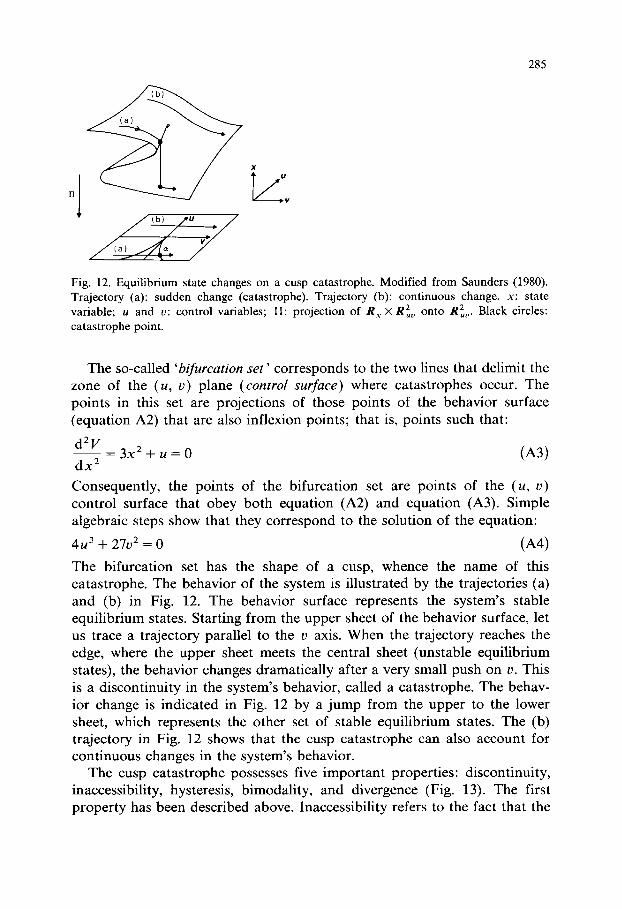
Fig. 12. Equilibrium state changes on a cusp catastrophe. Modified from Saunders (1980). Trajectory (a): sudden change (catastrophe). Trajectory (b): continuous change. x: state variable; u and v: control variables; II: projection of R, x Ri, onto Rz,. Black circles: catastrophe point.

The so-called ‘bifurcation set ’ corresponds to the two lines that delimit the zone of the (u, u) plane (control surface) where catastrophes occur. The points in this set are projections of those points of the behavior surface (equation A2) that are also inflexion points; that is, points such that:

d2V :=3x2+u=o (A3) dxL

\ I

Consequently, the points of the bifurcation set are points of the (u, u) control surface that obey both equation (A2) and equation (A3). Simple algebraic steps show that they correspond to the solution of the equation:

4u3 + 27u2 = 0 (A4) The bifurcation set has the shape of a cusp, whence the name of this catastrophe. The behavior of the system is illustrated by the trajectories (a) and (b) in Fig. 12. The behavior surface represents the system’s stable equilibrium states. Starting from the upper sheet of the behavior surface, let us trace a trajectory parallel to the u axis. When the trajectory reaches the edge, where the upper sheet meets the central sheet (unstable equilibrium states), the behavior changes dramatically after a very small push on u. This is a discontinuity in the system’s behavior, called a catastrophe. The behav- ior change is indicated in Fig. 12 by a jump from the upper to the lower sheet, which represents the other set of stable equilibrium states. The (b) trajectory in Fig. 12 shows that the cusp catastrophe can also account for continuous changes in the system’s behavior.

The cusp catastrophe possesses five important properties: discontinuity, inaccessibility, hysteresis, bimodality, and divergence (Fig. 13). The first property has been described above. Inaccessibility refers to the fact that the

286

\ / factor \

Fig. 13. Properties of the cusp catastrophe. Modified from Zeeman (1977). The unstable equilibrium sheet is not shown. x: state variable; ZJ and u: control variables; II: projection of R, X Rt, onto Ri,.

central sheet is formed of unstable equilibrium states, also called improbable behavior. To represent the property of inaccessibility, the central sheet has been removed in Fig. 13. Hysteresis results from the fact that the behavior stays on the surface sheet until it disappears, so that the jump from the upper to the lower sheet occurs at a different (u, u) point than the jump from the lower to the upper sheet (Fig. 13). Bimodality is shown by the fact that on the behavior surface in the cusp region, there are two possible behaviors for each point (u, u). The last property, divergence, refers to the fact that two trajectories on the behavior surface that start near each other in the neighborhood of the cusp point, and run parallel to the u axis, can end up one on the upper sheet and the other on the lower sheet.

Fig. 14. Example of a cusp with conflicting factors. Modified from Zeeman (1977). x: state variable; u and v: control variables; HI: projection of R, X Rt, onto R:,.

287

Generally, variable u is called the separation factor because the surface usually splits into upper and lower sheets along this axis. Variable u is then

called the normal factor. Variables u and u can also be called conflicting factors if they are oriented at an angle on each side of the bifurcation set, instead of cutting through it (Fig. 14).

REFERENCES

Bebars, M.I. and Lasserre, G., 1983. Analyse des p&cheries marines et lagunaires d’Egypte de 1962 a 1976 en liaison avec la construction du Haut Barrage. Acta Oecol., 6: 417-426.

Caumette, P. and Baleux, B., 1980. Etude des eaux rouges dues a la proliferation des batteries photosynthetiques sulfo-oxydantes dans P&tang du Prevost, lagune saumgtre mediter- raneenne. Mar. Biol., 56: 183-194.

Duckstein, L., Casti, J. and Kempf, J., 1979. Modelling phytoplankton dynamics using catastrophe theory. Water Resour. Res., 15: 1189-1194.

Gilmore, R., 1981. Catastrophe Theory for Scientists and Engineers. Wiley, New York, 666

PP. Gold, H.J., 1977. Mathematical Modelling of Biological Systems. An Introductory Guidebook.

Wiley-Interscience, New York, 357 pp. Harmsen, R., Rose, M.R. and Woodhouse, B., 1976. A general mathematical model for insect

outbreak. Proc. Entomol. Sot. Ont., 107: 11-18. Johnston, D.W. and Odum, E.P., 1956. Breeding bird populations in relation to plant

succession on the Piedmont of Georgia. Ecology, 37: 50-62. Kempf, J., 1980. Multiple steady states and catastrophes in ecological models. ISEM J., 2:

55-79. Legendre, P., Ouimet, C., Ross, G.J.S. and Vaudor, A., 1988. Testing the adjustment of a cusp

catastrophe model to data. Biometrics (submitted). Ouimet, C. and Brasselet, J.-P., 1985. Critiques sur un modele de dynamique du phytoplanc-

ton. Publ. IRMA, Vol. VII, Fast. 3, No. 6, Institut de Recherche Mathematique AvancCe,

27 PP. Poston, T. and Stewart, I., 1978. Catastrophe Theory and its Applications. Pitman, London,

491 pp. Rose, M.R. and Harmsen, R., 1981. Ecological outbreak dynamics and the cusp catastrophe.

Acta Biotheor., 30: 229-253. Salvadori, L. (Editor), 1984. Bifurcation Theory and Applications. Springer, Berlin, 233 pp. Saunders, P.T., 1980. An Introduction to Catastrophe Theory. Cambridge University Press,

Cambridge, 144 pp. Thorn, R., 1972. Stabilite Structurelle et Morphogenese: Essai d’une Theorie G&n&ale des

Modeles. Benjamin, Reading, MA, 362 pp. Thorn, R., 1975. Structural Stability and Morphogenesis; An Outline of a General Theory of

Models. Benjamin, Reading, MA, 348 pp. Williams, W.T., Lance, G.N., Webb, L.J., Tracey, J.G. and Dale, M.B., 1969. Studies in the

numerical analysis of complex rain-forest communities. III. The analysis of successional data. J. Ecol., 57: 515-535.

Zeeman, E.C., 1977. Catastrophe Theory: Selected papers, 1972-1977. Addison-Wesley, Reading, MA, 675 pp.