Embed Size (px)
Citation preview


A Pra ti al Companion to the ML Exer ise Book
An ML Pra ti al Companion Regression
1 Regression Methods
1. (Gradient des ent: omparison with
xxx another training algorithm
xxx on a fun tion approximation task)
• CMU, 2004 fall, Carlos Guestrin, HW4, pr. 2
In this problem you'll ompare the Gradient Des ent training algorithm with
one [other training algorithm of your hoosing, on a parti ular fun tion appro-
ximation problem. For this problem, the idea is to familiarize yourself with
Gradient Des ent and at least one other numeri al solution te hnique.
The dataset data.txt ontains a series of (x, y) re ords, where x ∈ [0, 5] and yis a fun tion of x given by y = a sin(bx)+w, where a and b are parameters to be
learned and w is a noise term su h that w ∼ N(0, σ2). We want to learn from
the data the best values of a and b to minimize the sum of squared error:
argmina,b
n∑
i=1
(yi − a sin(bxi))2.
Use any programming language of your hoi e and implement two training
te hniques to learn these parameters. The rst te hnique should be Gradient
Des ent with a xed learning rate, as dis ussed in lass. The se ond an be
any of the other numeri al solutions listed in lass: Levenberg-Marquardt,
Newton's Method, Conjugate Gradient, Gradient Des ent with dynami lear-
ning rate and/or momentum onsiderations, or one of your own hoi e not
mentioned in lass.
You may want to look at a s atterplot of the data to get rough initial values
for the parameters a and b. If you are getting a large sum of squared error
after onvergen e (where large means > 100), you may want to try random
restarts.
Write a short report detailing the method you hose and its relative perfor-
man e in omparison to standard Gradient Des ent (report the nal solution
obtained (values of a and b) and some measure of the omputation required
to rea h it and/or the resistan e of the approa h to lo al minima). If possi-
ble, explain the dieren e in performan e based on the algorithmi dieren e
between the two approa hes you implemented and the fun tion being learned.
2

Regression An ML Pra ti al Companion
2. (Distribuµia exponenµial : estimarea parametrilor
xxx în sens MLE ³i respe tiv în sens MAP,
xxx folosind a distribuµie a priori distribuµia Gamma)
CMU, 2015 fall, A. Smola, B. Po zos, HW1, pr. 1.1.ab
a. An exponential distribution with parameter λ has the probability density
fun tion (p.d.f.) Exp(x) = λe−λxfor x ≥ 0. Given some i.i.d. data xini=1 ∼
Exp(λ), derive the maximum likelihood estimate (MLE) λMLE
.
b. A Gamma distribution with parameters r > 0, α > 0 has the p.d.f.
Gamma(x|r, α) = αr
Γ(r)xr−1e−αx
for x ≥ 0,
where Γ is Euler's gamma fun tion.
If the posterior distribution is in the same family as the prior distribution,
then we say that the prior distribution is the onjugate prior for the likelihood
fun tion.
Show that the Gamma distribution is a onjugate prior of the Exp(λ) dis-
tribution. In other words, show that if Xnot.
= xini=1 and X ∼ Exp(λ) and
λ ∼ Gamma(r, α), then P (λ|X) ∼ Gamma(r∗, α∗) for some values r∗, α∗.
. Derive the maximum a posteriori estimator (MAP) λMAP
as a fun tion of
r, α.
d. What happens [with λMLE
and λMAP
as n gets large?
e. Let's perform an experiment in the above setting. Generate n = 20 random
variables drawn from Exp(λ = 0.2). Fix α = 100 and vary r over the range
(1, 30) using a stepsize of 1. Compute the orresponding MLE and MAP
estimates for λ. For ea h r, repeat this pro ess 50 times and ompute the
mean squared error of both estimates ompared against the true value. Plot
the mean squared error as a fun tion of r. (Note: O tave parameterizes the
Exponential distribution with θ = 1/λ.)
f. Now, x (r, α) = (30, 100) and vary n up to 1000. Plot the MSE for ea h n of
the orresponding estimates.
g. Under what onditions is the MLE estimator better? Under what ondi-
tions is the MAP estimator better? Explain the behavior in the two above
plots.
R spuns:
a. The log likelihood is
ℓ(λ) =∑
i
lnλ− λxi = nlogλ− λ∑
i
xi
Set the derivative to 0:
n
λ−∑
i
xi = 0⇒ λMLE
=1
x.
This is biased.
3

An ML Pra ti al Companion Regression
b.
P (λ|X) ∝ P (X |λ)P (λ)
∝ λne−λ∑
i xiλα−1e−βλ
∝ λn+α−1e−λ(∑
ixi+β).
Therefore P (λ|X) ∝ Gamma(α+ n,∑
i xi + β).
. The log posterior is
lnP (λ|X) ∝ −λ(
∑
i
xi + β
)
+ (n+ α− 1) lnλ.
Set the derivative to 0:
0 = −∑
i
xi − β +n+ α− 1
λ→ λ
MAP
=n+ α− 1∑
i xi + β.
d.
λMAP
=n+ α− 1∑
i xi + β=
1 +α− 1
n∑
i xi
n+
β
n
=1 +
α− 1
n
x+β
n
→ 1
x= λ
MLE
.
e.
f.
g. The MLE is better when prior information is in orre t. The MAP is better
with low sample size and good prior information. Asymptoti ally they are the
same.
4

Regression An ML Pra ti al Companion
3. (Distribuµia binomial : estimarea parametrului în sens MLE,
xxx folosind metoda lui Newton;
xxx distribuµia Gamma: estimarea parametrilor în sens MLE,
xxx folosind metoda gradientului ³i metoda lui Newton)
• CMU, 2008 spring, Tom Mit hell, HW2, pr. 1.2
xxx • CMU, 2015 fall, A. Smola, B. Po zos, HW1, pr. 1.2.
a. For the binomial sampling fun tion, pdf f(x) = Cxnp
x(1−p)n−x, nd the MLE
using the Newton-Raphson method, starting with an estimate θ0 = 0.1, n = 100,x = 8. Show the resulting θj until it rea hes onvergen e (θ
j+1−θj < .01). (Notethat the binomial pdf may be al ulated analyti ally - you may use this to
he k your answer.)
b. Note: For this [part of the exer ise, please make use of the digamma and
trigamma fun tions. You an nd the digamma and trigamma fun tions in
any s ienti omputing pa kage (e.g. O tave, Matlab, Python...).
Inside the handout, the estimators.mat le ontains a ve tor drawn from a
Gamma distribution. Run your implementation of gradient des ent and New-
ton's method for the later, see the ex. 120 in our exer ise book to obtain
the MLE estimators for this distribution. Create a plot showing the onver-
gen e of the two above methods. How do they ompare? Whi h took more
iterations? Lastly, provide the a tual estimated values obtained.
Solution:
a.
b. You should have gotten α ≈ 4, β ≈ 0.5.
5

An ML Pra ti al Companion Regression
4. (Linear, polynomial, regularized (L2), and kernelized regression:
xxx appli ation on a [UCI ML Repository dataset
xxx for housing pri es in Boston area)
• · MIT, 2001 fall, Tommi Jaakkola, HW1, pr. 1
xxx MIT, 2004 fall, Tommi Jaakkola, HW1, pr. 3
xxx MIT, 2006 fall, Tommi Jaakkola, HW2, pr. 2.d
A. Here we will be using a regression method to predi t housing pri es in
suburbs of Boston. You'll nd the data in the le housing.data. Information
about the data, in luding the olumn interpretation an be found in the le
housing.names. These les are taken from the UCI Ma hine Learning Repository
https://ar hive.i s.u i.edu/ml/datasets.html.
We will predi t the median house value (the 14th, and last, olumn of the
data) based on the other olumns.
a. First, we will use a linear regression model to predi t the house values,
using squared-error as the riterion to minimize. In other words y = f(x; w) =
w0 +∑13
i=1 wixi, where w = argminw∑n
t=1(yt − f(xt;w))2; here yt are the house
values, xt are input ve tors, and n is the number of training examples.
Write the following MATLAB fun tions (these should be simple fun tions to
ode in MATLAB):
• A fun tion that takes as input weights w and a set of input ve tors
xtt=1,...,n, and returns the predi ted output values ytt=1,...,n.
• A fun tion that takes as input training input ve tors and output values,
and return the optimal weight ve tor w.
• A fun tion that takes as input a training set of input ve tors and output
values, and a test set input ve tors, and output values, and returns the
mean training error (i.e., average squared-error over all training samples)
and mean test error.
b. To test our linear regression model, we will use part of the data set as a
training set, and the rest as a test set. For ea h training set size, use the rst
lines of the data le as a training set, and the remaining lines as a test set.
Write a MATLAB fun tion that takes as input the omplete data set, and the
desired training set size, and returns the mean training and test errors.
Turn in the mean squared training and test errors for ea h of the following
training set sizes: 10, 50, 100, 200, 300, 400.
(Qui k validation: For a sample size of 100, we got a mean training error of
4.15 and a mean test error of 1328.)
. What ondition must hold for the training input ve tors so that the training
error will be zero for any set of output values?
d. Do the training and test errors tend to in rease or de rease as the training
set size in reases? Why? Try some other training set sizes to see that this is
only a tenden y, and sometimes the hange is in the dierent dire tion.
e. We will now move on to polynomial regression. We will predi t the house
values using a fun tion of the form:
f(x;w) = w0 +
13∑
i=1
m∑
d=1
wi,d xdi ,
6

Regression An ML Pra ti al Companion
where again, the weights w are hosen so as to minimize the mean squared
error of the training set. Think about why we also in lude all lower order
polynomial terms up to the highest order rather than just the highest ones.
Note that we only use features whi h are powers of a single input feature.
We do so mostly in order to simplify the problem. In most ases, it is more
bene ial to use features whi h are produ ts of dierent input features, and
perhaps also their powers.
Think of why su h features are usually more powerful.
Write a version of your MATLAB fun tion from se tion b that takes as inputalso a maximal degree m and returns the training and test error under su h
a polynomial regression model.
NOTE : When the degree is high, some of the features will have extremely
high values, while others will have very low values. This auses severe nume-
ri pre ision problems with matrix inversion, and yields wrong answers. To
over ome this problem, you will have to appropriately s ale ea h feature xdi
in luded in the regression model, to bring all features to roughly the same
magnitude. Be sure to use the same s aling for the training and test sets.
For example, divide ea h feature by the maximum absolute value of the fe-
ature, among all training and test examples. (MATLAB matrix and ve tor
operations an be very useful for doing su h s aling operations easily.)
f.
g. For a training set size of 400, turn in the mean squared training and test
errors for maximal degrees of zero through ten.
(Qui k validation: for maximal degree two, we got a training error of 14.5 anda test error of 32.8).
h. Explain the qualitative behavior of the test error as a fun tion of the
polynomial degree. Whi h degree seems to be the best hoi e?
i. Prove (in two senten es) that the training error is monotoni ally de reasing
with the maximal degree m. That is, that the training error using a higher
degree and the same training set, is ne essarily less then or equal to the
training error using a lower degree.
j. We laim that if there is at least one feature ( omponent of the input
ve tor x) with no repeated values in the training set, then the training error
will approa h zero as the polynomial degree in reases. Why is this true?
B. In this [part of the problem, we explore the behavior of polynomial re-
gression methods when only a small amount of training data is available.
.
.
.
We will begin by using a maximum likelihood estimation riterion for the
parameters w that redu es to least squares tting.
k. Consider a simple 1D regression problem. The data in housing.data provides
information of how 13 dierent fa tors ae t house pri e in the Boston area.
(Ea h olumn of data represents a dierent fa tor, and is des ribed in brief
in the le housing.names.) To simplify matters (and make the problem easier to
7

An ML Pra ti al Companion Regression
visualise), we onsider predi ting the house pri e (the 14th olumn) from the
LSTAT feature (the 13th olumn).
We split the data set into two parts (in testLinear.m), train on the rst part
and test on the se ond. We have provided you with the ne essary MATLAB
ode for training and testing a polynomial regression model. Simply edit the
s ript (ps1_part2.m) to generate the variations dis ussed below.
i. Use ps1_part2.m to al ulate and plot training and test errors for
polynomial regression models as a fun tion of the polynomial order
(from 1 to 7). Use 250 training examples (set numtrain=250).
ii. Briey explain the qualitative behavior of the errors. Whi h of
the regression models are over-tting to the data? Provide a brief
justi ation.
iii. Rerun ps1 part2.m with only 50 training examples (set num-
train=50). Briey explain key dieren es between the resulting plot
and the one from part i). Whi h of the models are over-tting this
time?
Comment: There are many ways of trying to avoid over-tting. One way is
to use a maximum a posteriori (MAP) estimation riterion rather than maxi-
mum likelihood. The MAP riterion allows us to penalize parameter hoi es
that we would not expe t to lead to good generalization. For example, very
large parameter values in linear regression make predi tions very sensitive to
slight variations in the inputs. We an express a preferen e against su h large
parameter values by assigning a prior distribution over the parameters su h
as simple Gaussian
p(w;α2) = N (0, α2I).
This prior de reases rapidly as the parameters deviate from zero. The single
varian e (hyper-parameter) α2 ontrols the extent to whi h we penalize large
parameter values. This prior needs to be ombined with the likelihood to get
the MAP riterion. The MAP parameter estimate maximizes
ln(p(y|Xw, σ2) p(w;α2)) = ln p(y|Xw, σ2) + ln p(w;α2).
The resulting parameter estimates are biased towards zero due to the prior.
We an nd these estimates as before by setting the derivatives to zero.
l. Show that
wMAP
= (X⊤X +σ2
α2I)−1X⊤y.
m. In the above solution, show that in the limit of innitely large α, the MAP
estimate is equal to the ML estimate, and explain why this happens.
n. Let us see how the MAP estimate hanges our solution in the housing-pri e
estimation problem. The MATLAB ode you used above a tually ontains a
variable orresponding to the varian e ratio var_ratio =
α2
σ2for the MAP es-
timator. This has been set to a default value of zero to simulate the ML
estimator. In this part, you should vary this value from 1e-8 to 1e-4 in multi-
ples of 10 (i.e., 1e-8, 1e-7, . . . , 1e-4). A larger ratio orresponds to a stronger
prior (smaller values of α2 onstrain the parameters w to lie loser to origin).
8

Regression An ML Pra ti al Companion
iv. Plot the training and test errors as a fun tion of the polynomial
order using the above 5 MAP estimators and 250 and 50 training
points.
v. Des ribe how the prior ae ts the estimation results.
C. Implement the kernel linear regression method (des ribed in MIT, 2006
fall, Tommi Jaakkola, HW2, pr. 2.a- / Estimp-56 / Estimp-72) for λ > 0. We
are interested in exploring how the regularization parameter λ ≥ 0 ae ts thesolution when the kernel fun tion is the radial basis kernel
K(x, x′) = exp
(
−β
2‖x− x′‖2
)
, β > 0.
We have provided training and test data as well as helpful MATLAB s ripts
in hw2/prob2. You should only need to omplete the relevant lines in run prob2
s ript. The data pertains to the problem of predi ting Boston housing pri es
based on various indi ators (normalized). Evaluate and plot the training and
test errors (mean squared errors) as a fun tion of λ in the range λ ∈ (0, 1). Useβ = 0.05. Explain the qualitative behavior of the two urves.
Solution:
A.
a.
b. First to read the data (ignoring olumn four):
data = load('housing.data');
x = data(:,[1:3 5:13);
y = data(:,14);
To get the training and test errors for training set of size s, we invoke the
following MATLAB ommand:
[trainE,testE = testLinear(x,y,s)
Here are the errors I got:
training size training error test error
10 6.27× 10⁻²⁶ 1.05× 10⁵
50 3.437 24253100 4.150 1328200 9.538 316.1300 9.661 381.6400 22.52 41.23
[ Note that for a training size of ten, the training error should have been
zero. The very low, but still non-zero, error is a result of limited pre ision of
the al ulations, and is not a problem. Furthermore, with only ten training
examples, the optimal regression weights are not uniquely dened. There is a
four dimensional linear subspa e of weight ve tors that all yield zero training
error. The test error above (for a training size of ten) represents an 2arbitrary
hoi e of weights from this subspa e (impli itly made by the pinv() fun tion).
Using dierent, equally optimal, weights would yield dierent test errors.
9

An ML Pra ti al Companion Regression
. The training error will be zero if the input ve tors are linearly independent.
More pre isely, sin e we are allowing an ane term w0, it is enough that
the input ve tors with an additional term always equal to one, are linearly
independent. Let X be the matrix of input ve tors, with additional `one'
terms, y any output ve tor, and w a possible weight ve tor. If the inputs are
linearly independent, Xw = y always has a solution, and the weights w lead to
zero training error.
[ Note that if X is a square matrix with linearly independent rows, than it
is invertible, and Xw = y has a unique solution. But even if X is not square
matrix, but its rows are still linearly independent (this an only happen if
there are less rows then olumns, i.e., less features then training examples),
then there are solutions to Xw = y, whi h do not determine w uniquely, but
still yield zero training error (as in the ase of a sample size of ten above).
d. The training error tends to in rease. As more examples have to be tted,
it be omes harder to 'hit', or even ome lose, to all of them.
The test error tends to de rease. As we take into a ount more examples
when training, we have more information, and an ome up with a model that
better resembles the true behavior. More training examples lead to better
generalization.
e. We will use the following fun tions, on top of those from question b:
fun tion xx = degexpand(x, deg)
fun tion [trainE, testE = testPoly(x, y, numtrain, deg)
f.
.
.
.
g. To get the training and test errors for maximum degree d, we invoke the
following MATLAB ommand:
[trainE,testE = testPoly(x,y,400,d)
Here are the errors I got:
degree training error test error
0 83.8070 102.22661 22.5196 41.22852 14.8128 32.83323 12.9628 31.78804 10.8684 52625 9.4376 50676 7.2293 4.8562× 10⁷
7 6.7436 1.5110× 10⁶
8 5.9908 3.0157× 10⁹
9 5.4299 7.8748× 10¹⁰
10 4.3867 5.2349× 10¹³
[ These results were obtained using pinv(). Using dierent operations, although
theoreti ally equivalent, might produ e dierent results for higher degrees. In
any ase, using any of the suggested methods above, the errors should mat h
the above table at least up to degree ve. Beyond that, using inv() starts
produ ing unreasonable results due to extremely small values in the matrix,
10

Regression An ML Pra ti al Companion
whi h make it almost singular (non-invertible). If you used inv() and got su h
values, you should point this out.
Degree zero refers to having a onstant predi tor, i.e., predi t the same input
value for all output values. The onstant value that minimizes the training
error (and is thus used) is the mean training output.
h. Allowing more omplex models, with more features, we an use as predi -
tors fun tions that better orrespond to the true behavior of the data. And
so, the approximation error (the dieren e between the optimal model from
our limited lass, and the true behavior of the data) de reases as we in rease
the degree. As long as there is enough training data to support su h omplex
models, the generalization error is not too bad, and the test error de rea-
ses. However, past some point we start over-tting the training data and
the in rease in the generalization error be omes mu h more signi ant than
the ontinued de rease in the approximation error (whi h we annot dire tly
observe), ausing the test error to rise.
Looking at the test error, the best maximum degree seems to be three.
i. Predi tors of lower maximum degree are in luded in the set of predi tors
of higher maximum degree (they orrespond to predi tors in whi h weights
of higher degree features are set to zero). Sin e we hoose the predi tor from
within the set the minimizes the training error, allowing more predi tors, an
only de rease the training error.
j. We show for all m ≥ n − 1 (where n is the number of training examples),
the training error is 0, but onstru ting weights whi h predi t the training
examples exa tly. Let j be a omponent of the input with no repeat values.
We let wi,d = 0 for all i = j, and all d = 1, . . . ,m. Then we have
f(x) = w0 +∑
i
∑
d
wi,dxdi = w0 +
m∑
d=1
wj,dxdj .
Given n training points (x1, y1), . . . , (xn, yn) we are required to nd w0, wj,1, . . . , wj,m
s.t. w0 +∑m
d=1wj,d(xi)dj = yi, ∀i = 1, . . . , n. That is, we want to interpolate n po-
ints with a degree m ≥ n− 1 polynomial, whi h an be done exa tly as long as
the points xi are distin t.
B.
k.
i.
ii. The training error is monotoni ally de reasing (non-in reasing) with po-
lynomial order. This is be ause higher order models an fully represent any
11

An ML Pra ti al Companion Regression
lower order model by adequate setting of parameters, whi h in turn implies
that the former an do no worse than the latter when tting to the same
training data.
(Note that this monotoni ity property need not hold if the training sets to
whi h the higher and lower order models were t were dierent, even if these
were drawn from the same underlying distribution.)
The test error mostly de reases with model order till about 5th order, and
then in reases. This is an indi ation (but not proof) that higher order models
(6th and 7th) might be overtting to the data. Based on these results, the
best hoi e of model for training on the given data is the 5th order model,
sin e it has lowest error on an independent test set of around 250 examples.
iii.
We note the following dieren es between the plots for 250 and 50 examples:
• The training errors are lower in the present ase. This is be ause we
are having to t fewer points with the same model. In this examples, in
parti ular, we are tting only a subset of the points we were previously
tting (sin e there is no randomness in drawing points for training).
• The test errors for most models are higher. This is eviden e of systemati
overtting for all model orders, relative to the ase where there were many
more training points.
• The model with the lowest test error is now the third order model. From
4th order onwards, the test error generally in reases (though the 7th order
is an ex eption, perhaps due to the parti ular hoi e of training and test
sets). This tells us that with fewer training examples, our preferen e
should swit h towards lower-order models (in the interest of a hieving
low generalisation error), even though the true model responsible for
generating the underlying data might be of mu h higher order. This
relates to the trade-o between bias and varian e. We typi ally want
to minimise the mean-square error, whi h is the sum of the bias and
varian e. Low-order models typi ally have high bias but low varian e.
Higher order models may be unbiased, but have higher varian e.
l.
.
.
.
m.
.
.
.
n.
12

Regression An ML Pra ti al Companion
iv.
Plots for 250 training examples. Left to right, (then) top to bottom, varian e
ratio = 1e-8 to 1e-4:
Plots for 50 training examples. Left to right, (then) top to bottom, varian e
ratio = 1e-8 to 1e-4:
v. We make the following observations:
• As the varian e ratio (i.e. the strength of the prior) in reases, the trai-
ning error in reases (slightly). This is be ause we are no longer solely
interested in obtaining the best t to the training data.
• The test error for higher order models de reases dramati ally with strong
priors. This is be ause we are no longer allowing these models to overt
to training data by restri ting the range of weights possible.
• Test error generally de reases with in reasing prior.
13

An ML Pra ti al Companion Regression
• As a onsequen e of the above two points, the best model hanges slightly
with in reasing prior in the dire tion of more omplex models.
• For 50 training samples, the dieren e in test error between ML and
MAP is more signi ant than with 250 training examples. This is be ause
overtting is a more serious problem in the former ase.
C. Sample ode for this problem is shown below:
Ntrain = size(Xtrain,1);
Ntest = size(Xtest,1);
for i=1:length(lambda),
lmb = lambda(i);
alpha = lmb * ((lmb*eye(Ntrain) + K)
∧-1) * Ytrain;
Atrain = (1/lmb) * repmat( alpha', Ntrain, 1);
yhat_train = sum(Atrain.*K,2);
Atest = (1/lmb) * repmat( alpha', Ntest, 1);
yhat_test = sum(Atest.*(Ktrain_test'), 2);
E(i,:) = [mean((yhat_train-Ytrain).
∧2),mean((yhat_test-Ytest).
∧2);
end;
The resulting plot is shown in the
nearby gure. As an be seen the
training error is zero at λ = 0 and
in reases as λ in reases. The test er-
ror initially de reases, rea hes a mi-
nimum around 0.1, and then in rea-
ses again. This is exa tly as we would
expe t.
λ ≈ 0 results in over-tting (the mo-
del is too powerful). Our regression
fun tion has a low bias but high va-
rian e.
By in reasing λ we onstrain the mo-
del, thus in reasing the training er-
ror. While the regularization in rea-
ses bias, the varian e de reases fas-
ter, and we generalize better.
High values of λ result in under-
tting (high bias, low varian e) and
both training error and test errors
are high.
14

Regression An ML Pra ti al Companion
5. (Regresia liniar lo al-ponderat regularizat , kernel-izat )
• Stanford, 2008 fall, Andrew Ng, HW1, pr. 2.d
The les q2x.dat and q2y.dat ontain the inputs (x(i)) and outputs (y(i)) for aregression problem, with one training example per row.
a. Implement (unweighted) linear regression (y = θ⊤x) on this dataset (using
the normal equations, [LC: i.e., the analyti al / losed form solution), and
plot on the same gure the data and the straight line resulting from your t.
(Remember to in lude the inter ept term.)
b. Implement lo ally weighted linear regression on this dataset (using the
weighted normal equations you derived in part (b) [LC: i.e, Stanford, 2008
fall, Andrew Ng, HW1, pr. 2.b, but you may take a look at CMU, 2010 fall,
Aarti Singh, midterm, pr. 4 found in the exer ise book), and plot on the same
gure the data and the urve resulting from your t. When evaluating h( · )at a query point x, use weights
w(x(i)) = exp
(
− (x− x(i))2
2τ2
)
,
with a bandwidth parameter τ = 0.8. (Again, remember to in lude the inter-
ept term.)
. Repeat (b) four times, with τ = 0.1, 0.3, 2 and 10. Comment briey on what
happens to the t when τ is too small or too large.
Solution:
LC: See the ode in the prob2.m Matlab le that I put in the HW1 sub-
folder of Stanford 2011f folder in the main (Stanford) arhive and also in
book/g/Stanford.2008f.ANg.HW1.pr2d.
15

An ML Pra ti al Companion Regression
(Plotted in olor where available.)
For small bandwidth parameter τ , the tting is dominated by the losest by
training samples. The smaller the bandwidth, the less training samples that
are a tually taken into a ount when doing the regression, and the regression
results thus be ome very sus eptible to noise in those few training samples.
For larger τ , we have enough training samples to reliably t straight lines,
unfortunately a straight line is not the right model for these data, so we also
get a bad t for large bandwidths.
16

Regression An ML Pra ti al Companion
6. ([Weighted Linear Regression applied to
xxx predi ting the needed quatity of insulin,
xxx starting from the sugar level in the patient's blood)
• CMU, 2009 spring, Ziv Bar-Joseph, HW1, pr. 4
An automated insulin inje tor needs to al ulate how mu h insulin it should
inje t into a patient based on the patient's blood sugar level. Let us formulate
this as a linear regression problem as follows: let yi be the dependent predi tedvariable (blood sugar level), and let β0, β1 and β2 be the unknown oe ients
of the regression fun tion. Thus, yi = β0 + β1xi + β2x2i , and we an formulate
the problem of nding the unknown βnot.
= (β0, β1, β2) as:
β = (X⊤X)−1X⊤y.
See data2.txt (posted on website) for data based on the above s enario with
spa e separated elds onforming to:
bloodsugarlevel insulinedose weightage
The purpose of the weightage eld will be made lear in part c.
a. Write ode in Matlab to estimate the regression oe ients given the
dataset onsisting of pairs of independent and dependent variables. Generate
a spa e separated le with the estimated parameters from the entire dataset
by writing out all the parameter.
b. Write ode in Matlab to perform inferen e by predi ting the insulin dosage
given the blood sugar level based on training data using a leave one out ross
validation s heme. Generate a spa e separated le with the predi ted dosages
in order. The predi ted dosages:
. However, it has been found that one group of patients are twi e as sensitive
to the insuline dosage than the other. In the training data, these parti ular
patients are given a weightage of 2, while the others are given a weightage
of 1. Is your goodness of t fun tion exible enough to in orporate this
information?
d. Show how to formulate the regression fun tion, and orrespondingly al-
ulate the oe ients of regression under this new s enario, by in orporating
the given weights.
e. Code up this variant of regressional analysis. Write out the new oe ients
of regression you obtain by using the whole dataset as training data.
Solution:
a. The betas, in order:
−74.3825 13.4215 1.1941
b.
1417.0177 1501.4423 1966.3563 2833.7942 2953.4532 3075.472 3199.8566 3326.96633456.4704 5038.3777 5196.6767 5357.0094 7091.8113 7278.2709 7467.3604 7658.52567852.0808 9703.9748 9921.8604 10142.5438 10365.8512 12498.2968 12749.6202 13003.941798.3745 1869.1966 2024.7112 2265.6988 2392.0227 2756.1588 3915.9302 4004.4654878.0057 5094.3282 6217.981 6485.8542 6544.4688 6805.7564 7073.8455 7207.50327285.3657 9393.5129 9515.9043 9704.0029 10060.5539 12037.6304 12361.3586 12903.5394
17

An ML Pra ti al Companion Regression
. Sin e we need to weigh ea h point dierently, out urrent goodness of t
fun tion is unable to work in this s enario. However, sin e the weights for this
spe i dataset are 1 and 2, we may just use the old formalism and double
the data items with weightage 2. The hanged formalism whi h enables us to
assign weights of any pre ision to the data sample is shown below.
d. Let:
y = Xβ
y = (y1, y2, . . . , yn)⊤
β = (β1, β2, . . . , βm)⊤
Xi,1 = 1
Xi,j+1 = xi,j
Let us dene the weight matrix as:
Ωi,i =√wi
Ωi,j = 0 (for i 6= j)So, Ωy = ΩXβ.
To minimize the weighted square error, we have to take the derivative with
respe t to β:
∂
∂β((Ωy − ΩXβ)⊤(Ωy − ΩXβ))
=∂
∂β((Ωy)⊤(Ωy)− 2(Ωy)⊤(ΩXβ) + (ΩXβ)⊤(ΩXβ)
=∂
∂β((Ωy)⊤(Ωy)− 2(Ωy)⊤(ΩXβ) + β⊤X⊤Ω⊤ΩXβ
Therefore
∂
∂β((Ωy − ΩXβ)⊤(Ωy − ΩXβ)) = 0
⇔ 0− 2((Ωy)⊤(ΩX))⊤ + 2X⊤Ω⊤ΩXβ = 0
⇔ β = (X⊤Ω⊤ΩX)−1X⊤Ω⊤Ωy
e. The new beta oe ients are in order:
−57.808 13.821 1.199
18

Regression An ML Pra ti al Companion
7. (Linear [Ridge regression applied to
xxx predi ting the level of PSA in the prostate gland,
xxx using a set of medi al test results)
• ⋆ ⋆ CMU, 2009 fall, Geo Gordon, HW3, pr. 3
The linear regression method is widely used in the medi al domain. In this
question you will work on a prostate an er data from a study by Stamey et
al.
697
You an download the data from . . . .
Your task is to predi t the level of prostate-spe i antigen (PSA) using a set
of medi al test results. PSA is a protein produ ed by the ells of the prostate
gland. High levels of PSA often indi ate the presen e of prostate an er or
other prostate disorders.
The attributes are several lini al measurements on men who have prostate
an er. There are 8 attributes: log an er volume l avol, log prostate weight
(lweight), log of the amount of benign prostati hyperplasia (lbph), seminal
vesi le invasion (svi), age, log of apsular penetration (l p), Gleason s ore
(gleason), and per ent of Gleason s ores of 4 or 5 (pgg45). svi and gleason
are ategori al, that is they take values either 1 or 0; others are real-valued.
We will refer to these attributes as A1 = l avol, A2 = lweight, A3 = age, A4
= lbph, A5 = svi, A6 = l p, A7 = gleason, A8 = pgg45.
Ea h row of the input le des ribes one data point: the rst olumn is the
index of the data point, the following eight olumns are attributes, and the
tenth olumn gives the log PSA level lpsa, the response variable we are in-
terested in. We already randomized the data and split it into three parts
orresponding to training, validation and test sets. The last olumn of the le
indi ates whether the data point belongs to the training set, validation set
or test set, indi ated by `1' for training, `2' for validation and `3' for testing.
The training data in ludes 57 examples; validation and test sets ontain 20
examples ea h.
Inspe ting the Data
a. Cal ulate the orrelation matrix of the 8 attributes and report it in a table.
The table should be 8-by-8. You an use Matlab fun tions.
b. Report the top 2 pairs of attributes that show the highest pairwise positive
orrelation and the top 2 pairs of attributes that show the highest pairwise
negative orrelation.
Solving the Linear Regression Problem
You will now try to nd several models in order to predi t the lpsa levels.
The linear regression model is
Y = f(X) + ǫ
where ǫ is a Gaussian noise variable, and
f(X) =
p∑
j=0
wjφj(X)
697
Stamey TA, Kabalin JN, M Neal JE et al. Prostate spe i antigen in the diagnosis and treatment of the
prostate. II. Radi al prostate tomy treated patients. J Urol 1989;141:107683.
19
An ML Pra ti al Companion Regression
where p is the number of basis fun tions (features), φj is the jth basis fun tion,and wj is the weight we wish to learn for the jth basis fun tion. In the models
below, we will always assume that φ0(X) = 1 represents the inter ept term.
. Write a Matlab fun tion that takes the data matrix Φ and the olumn
ve tor of responses y as an input and produ es the least squares t w as the
output (refer to the le ture notes for the al ulation of w).
d. You will reate the following three models. Note that before solving ea h
regression problem below, you should s ale ea h feature ve tor to have a
zero mean and unit varian e. Don't forget to in lude the inter ept olumn,
φ0(X) = 1, after s aling the other features. Noti e that sin e you shifted the
attributes to have zero mean, in your solutions, the inter ept term will be the
mean of the response variable.
• Model1: Features are equal to input attributes, with the addition of a on-
stant feature φ0. That is, φ0(X) = 1, φ1(X) = A1, . . . , φ8(X) = A8. Solve the
linear regression problem and report the resulting feature weights. Dis uss
what it means for a feature to have a large negative weight, a large positive
weight, or a small weight. Would you be able to omment on the weights, if
you had not s aled the predi tors to have the same varian e? Report mean
squared error (MSE) on the training and validation data.
• Model2: In lude additional features orresponding to pairwise produ ts of
the rst six of the original attributes,
698
i.e., φ9(X) = A1·A2, . . . , φ13(X) = A1·A6,
φ15(X) = A2 · A3, . . . , φ23(X) = A5 · A6. First ompute the features a ording
to the formulas above using the unnormalized values, then shift and s ale the
new features to have zero mean and unit varian e and add the olumn for the
inter ept term φ0(X) = 1. Report the ve features whose weights a hieved the
largest absolute values.
• Model3: Starting with the results of Model1, drop the four features with
the lowest weights (in absolute values). Build a new model using only the
remaining features. Report the resulting weights.
e. Make two bar harts, the rst to ompare the training errors of the three
models, the se ond to ompare the validation errors of the three models.
Whi h model a hieves the best performan e on the training data? Whi h
model a hieves the best performan e on the validation data? Comment on
dieren es between training and validation errors for individual models.
f. Whi h of the models would you use for predi ting the response variable?
Explain.
Ridge Regression
For this question you will start with Model2 and employ regularization on it.
g. Write a Matlab fun tion to solve Ridge regression. The fun tion should take
the data matrix Φ, the olumn ve tor of responses y, and the regularization
parameter λ as the inputs and produ e the least squares t w as the output
(refer to the le ture notes for the al ulation of w). Do not penalize w0, the
698
These features are also alled intera tions, be ause they attempt to a ount for the ee t of two attributes
being simultaneously high or simultaneously low.
20

Regression An ML Pra ti al Companion
inter ept term. (You an a hieve this by repla ing the rst olumn of the λImatrix with zeros.)
h. You will reate a plot exploring the ee t of the regularization parameter
on training and validation errors. The x-axis is the regularization parameter
(on a log s ale) and the y-axis is the mean squared error. Show two urves in
the same graph, one for the training error and one for the validation error.
Starting with λ = 2−30, try 50 values: at ea h iteration in rease λ by a fa tor
of 2, so that for example the se ond iteration uses λ = 2−29. For ea h λ, you
need to train a new model.
i. What happens to the training error as the regularization parameter in-
reases? What about the validation error? Explain the urve in terms of
overtting, bias and varian e.
j. What is the λ that a hieves the lowest validation error and what is the
validation error at that point? Compare this validation error to the Model2
validation error when no regularization was applied (you solved this in part
e). How does w dier in the regularized and unregularized versions, i.e., what
ee t did regularization have on the weights?
k. Is this validation error lower or higher than the validation error of the
model you hose in part f? Whi h one should be your nal model?
l. Now that you have de ided on your model (features and possibly the re-
gularization parameter), ombine your training and validation data to make
a ombined training set, train your model on this ombined training set, and
al ulate it on the test set. Report the training and test errors.
Solution:
a.
l avol lweight age lbph svi l p gleason pgg45 lpsa
l avol 1.0000 0.2805 0.2249 0.0273 0.5388 0.6753 0.4324 0.4336 0.7344
lweight 0.2805 1.0000 0.3479 0.4422 0.1553 0.1645 0.0568 0.1073 0.4333
age 0.2249 0.3479 1.0000 0.3501 0.1176 0.1276 0.2688 0.2761 0.1695
lbph 0.0273 0.4422 0.3501 1.0000 -0.0858 -0.0069 0.0778 0.0784 0.1798
svi 0.5388 0.1553 0.1176 -0.0858 1.0000 0.6731 0.3204 0.4576 0.5662
l p 0.6753 0.1645 0.1276 -0.0069 0.6731 1.0000 0.5148 0.6315 0.5488
gleason 0.4324 0.0568 0.2688 0.0778 0.3204 0.5148 1.0000 0.7519 0.3689
pgg45 0.4336 0.1073 0.2761 0.0784 0.4576 0.6315 0.7519 1.0000 0.4223
lpsa 0.7344 0.4333 0.1695 0.1798 0.5662 0.5488 0.3689 0.4223 1.0000
b. The top 2 pairs that show the highest pairwise positive orrelation are
gleason - ppg4 (0.7519) and l avol -l p (0.6731). Highest negative orrelations:
lbph - svi (-0.0858) and lph - l p (-0.0070).
. See below:
fun tion what=lregress(Y,X)
% least square solution to linear regression
% X is the feature matrix
% Y is the response variable ve tor
what=inv(X'*X)*X'*Y;
end
d.
Model1:
21

An ML Pra ti al Companion Regression
the weight ve tor:
w = [2.68265, 0.71796, 0.17843,−0.21235, 0.25752, 0.42998,−0.14179, 0.08745, 0.02928].Model2:
The largest ve absolute values in des ending order:
lweight*age, lpbh, lweight, age, age*lpbh.
Model3:
The features with have the lowest absolute weights in Model1:
pgg45, gleason, l p, lweight.
The resulting weights: w = [2.6827, 0.7164,−0.1735, 0.3441, 0.4095].
e.
1 2 30
0.1
0.2
0.3
0.4
0.5
0.6
0.7Training Error of the Three Models
Model ID
Tra
inin
g M
SE
1 2 30
0.2
0.4
0.6
0.8
1Validation Error of the Three Models
Model ID
Val
idat
ion
MS
E
Model2 a hieves the best performan e on the training data, whereas Model1
a hieves the best performan e on the validation data. Model2 suer from
overtting, indi ated by the very good training model but low validation error.
Model3 seems to be too simple, it has a higher training and a higher validation
error ompared to Model1. The features that are dropped are informative, as
indi ated by the lower training and validation errors.
f. Model1, sin e it a hieves the best performan e on the validation data.
Model2 overts, and Model3 is too simple.
g. See below:
fun tion what = ridgeregress(Y,X,lambda)
% X is the feature matrix
% Y is the response ve tor
% what are the estimated weights
penal = lambda*eye(size(X,2));
penal(:,1) = 0;
what = inv(X'*X+penal)*X'*Y;
end
22

Regression An ML Pra ti al Companion
h.
−30 −20 −10 0 10 200.2
0.4
0.6
0.8
1
1.2
1.4
1.6
log2(lambda)
MS
E
training errortesting error
i. When the model is not regularized mu h (the left side of the graph), the
training error is low and the validation error is high, indi ating the model is
too omplex and overtting to the training data. In that region, the bias is
low and the varian e is high.
As the regularization parameter in reases, the bias in reases and varian e
de reases. The overtting problem is over ome as indi ated by de reasing
validation error and in reasing training error.
As regularization penalty in rease too mu h, the model be omes getting too
simple and start suering from undertting as an be shown by the poor
performan e on the training data.
j. logλ = 4, i.e., λ = 16, a hieves the lowest validation error, whi h is 0.447.
This validation error is mu h less than the validation error of the model wi-
thout regularization, whi h was 0.867. Regularized weights are smaller than
unregularized weights. Regularization de reases the magnitude of the weights.
k. The validation error of the penalized model (λ = 16) is 0.447, whi h is lowerthan Model1's validation error, 0.5005. Therefore, this model is hosen.
l. The nal models' training error is 0.40661 and the test error is 0.58892.
23

An ML Pra ti al Companion Regression
8. (Linear weighted, unweighted, and fun tional regression:
xxx appli ation to denoising quasar spe tra)
• · Stanford, 2017 fall, Andrew Ng, Dan Boneh, HW1, pr. 5
xxx Stanford, 2016 fall, Andrew Ng, John Du hi, HW1, pr. 5
Solution:
24

Regression An ML Pra ti al Companion
9. ([Feature sele tion in the ontext of linear regression
xxx with L1 regularization:
xxx the oordinate des ent method)
• ⋆ MIT, 2003 fall, Tommi Jaakkola, HW4, pr. 1
Solution:
25

An ML Pra ti al Companion Regression
10. (Logisti regression with gradient as ent:
xxx appli ation to text lassi ation)
• CMU, 2010 fall, Aarti Singh, HW1, pr. 5
In this problem you will implement Logisti Regression and evaluate its per-
forman e on a do ument lassi ation task. The data for this task is taken
from the 20 Newsgroups data set,
699
and is available from the ourse web
page.
Our model will use the bag-of-words assumption. This model assumes that
ea h word in a do ument is drawn independently from a ategori al distribu-
tion over possible words. (A ategori al distribution is a generalization of a
Bernoulli distribution to multiple values.) Although this model ignores the
ordering of words in a do ument, it works surprisingly well for a number of
tasks. We number the words in our vo abulary from 1 to m, where m is the
total number of distin t words in all of the do uments. Do uments from lass
y are drawn from a lass-spe i ategori al distribution parameterized by θy.θy is a ve tor, where θy,i is the probability of drawing word i and
∑mi=1 θy,i = 1.
Therefore, the lass- onditional probability of drawing do ument x from our
model is
P (X = x|Y = y) =m∏
i=1
θ ounti(x)y,i ,
where ounti(x) is the number of times word i appears in x.
a. Provide high-level des riptions of the Logisti Regression algorithm. Be
sure to des ribe how to estimate the model parameters and how to lassify a
new example.
b. Implement Logisti Regression. We found that a step size around 0.0001
worked well. Train the model on the provided training data and predi t the
labels of the test data. Report the training and test error.
Solution:
a. The logisti regression model is
P (Y = 1|X = x,w) =exp(w0 +
∑
i wixi)
1 + exp(w0 +∑
iwixi),
where w = (w0, w1, . . . , wm)⊤ is our parameter ve tor. We will nd w by maxi-
mizing the data loglikelihood l(w):
l(w) = log
∏
j
exp(yj(w0 +∑
i wixji ))
1 + exp(w0 +∑
i wixji )
=∑
j
(
yj(w0 +∑
i
wixji )− log(1 + exp(w0 +
∑
i
wixji ))
)
We an estimate/learn the parameters (w) of logisti regression by optimi-
zing l(w), using gradient as ent. The gradient of l(w) is the array of partial
derivatives of l(w):
699
Full version available from http://people. sail.mit.edu/jrennie/20Newsgroups/.
26
Regression An ML Pra ti al Companion
∂l(w)
∂w0=
∑
j
(
yj − exp(w0 +∑
iwixji )
1 + exp(w0 +∑
iwixji )
)
=∑
j
(yj − P (Y = 1|X = xj ;w))
∂l(w)
∂wk=
∑
j
(
yjxjk −
xjk exp(w0 +
∑
i wixji )
1 + exp(w0 +∑
iwixji )
)
=∑
j
xjk(y
j − P (Y = 1|X = xj ;w))
Let w(t)represent our parameter ve tor on the t-th iteration of gradient as ent.
To perform gradient as ent, we rst set w(0)to some arbitrary value (say 0).
We then repeat the following updates until onvergen e:
w(t+1)0 ← w
(t)0 + α
∑
j
(
yj − P (Y = 1|X = xj ;w(t)))
w(t+1)k ← w
(t)k + α
∑
j
xjk
(
yj − P (Y = 1|X = xj ;w(t)))
where α is a step size parameter whi h ontrols how far we move along our
gradient at ea h step. We set α = 0.0001. The algorithm onverges when
||w(t)−w(t+1)|| < δ, that is when the weight ve tor doesn't hange mu h during
an iteration. We set δ = 0.001.
b. Training error: 0.00. Test error: 0.29. The large dieren e between trainingand test error means that our model overts our training data. A possible
reason is that we do not have enough training data to estimate either model
a urately.
27

An ML Pra ti al Companion Regression
11. (Logisti regression with gradient as ent:
xxx appli ation on a syntheti dataset from R2;
xxx overtting)
• CMU, 2015 spring, T. Mit hell, N. Bal an, HW4, pr. 2. -i
In logisti regression, our goal is to learn a set of parameters by maximizing
the onditional log-likelihood of the data.
In this problem you will implement a logisti regression lassier and apply it
to a two- lass lassi ation problem. In the ar hive, you will nd one .m le
for ea h of the fun tions that you are asked to implement, along with a le
alled HW4Data.mat that ontains the data for this problem. You an load the
data into O tave by exe uting load(HW4Data.mat) in the O tave interpreter.
Make sure not to modify any of the fun tion headers that are provided.
a. Implement a logisti regression lassier using gradient as ent for the
formulas and their al ulation see ex. 12 in our exer ise book
700
by lling
in the missing ode for the following fun tions:
• Cal ulate the value of the obje tive fun tion:
obj = LR_Cal Obj(XTrain,yTrain,wHat)
• Cal ulate the gradient:
grad = LR_Cal Grad(XTrain,yTrain,wHat)
• Update the parameter value:
wHat = LR_UpdateParams(wHat,grad,eta)
• Che k whether gradient as ent has onverged:
hasConverged = LR_Che kConvg(oldObj,newObj,tol)
• Complete the implementation of gradient as ent:
[wHat,objVals = LR_GradientAs ent(XTrain,yTrain)
• Predi t the labels for a set of test examples:
[yHat,numErrors = LR_Predi tLabels(XTest,yTest,wHat)
where the arguments and return values of ea h fun tion are dened as follows:
• XTrain is an n × p dimensional matrix that ontains one training instan e
per row
• yTrain is an n × 1 dimensional ve tor ontaining the lass labels for ea h
training instan e
• wHat is a p+1× 1 dimensional ve tor ontaining the regression parameter
estimates w0, w1, . . . , wp
• grad is a p+ 1× 1 dimensional ve tor ontaining the value of the gradient
of the obje tive fun tion with respe t to ea h parameter in wHat
• eta is the gradient as ent step size that you should set to eta = 0.01
• obj, oldObj and newObj are values of the obje tive fun tion
• tol is the onvergen e toleran e, whi h you should set to tol = 0.001
• objVals is a ve tor ontaining the obje tive value at ea h iteration of gra-
dient as ent
700
From the formal point of view you will assume that a dataset with n training examples and p features will be
given to you. The lass labels will be denoted y(i), the features x(i)1 , . . . , x
(i)p , and the parameters w0, w1, . . . , wp,
where the supers ript (i) denotes the sample index.
28
Regression An ML Pra ti al Companion
• XTest is an m × p dimensional matrix that ontains one test instan e per
row
• yTest is an m × 1 dimensional ve tor ontaining the true lass labels for
ea h test instan e
• yHat is an m× 1 dimensional ve tor ontaining your predi ted lass labels
for ea h test instan e
• numErrors is the number of mis lassied examples, i.e. the dieren es be-
tween yHat and yTest
To omplete the LR_GradientAs ent fun tion, you should use the helper fun -
tions LR_Cal Obj, LR_Cal Grad, LR_UpdateParams, and LR_Che kConvg.
b. Train your logisti regression lassier on the data provided in XTrain and
yTrain with LR_GradientAs ent, and then use your estimated parameters wHat to
al ulate predi ted labels for the data in XTest with LR_Predi tLabels.
. Report the number of mis lassied examples in the test set.
d. Plot the value of the obje tive fun tion on ea h iteration of gradient des-
ent, with the iteration number on the horizontal axis and the obje tive value
on the verti al axis. Make sure to in lude axis labels and a title for your
plot. Report the number of iterations that are required for the algorithm to
onverge.
e. Next, you will evaluate how the training and test error hange as the trai-
ning set size in reases. For ea h value of k in the set 10, 20, 30, . . . , 480, 490, 500,rst hoose a random subset of the training data of size k using the following
ode:
subsetInds = randperm(n, k)
XTrainSubset = XTrain(subsetInds, :)
yTrainSubset = yTrain(subsetInds)
Then re-train your lassier using XTrainSubset and yTrainSubset, and use the
estimated parameters to al ulate the number of mis lassied examples on
both the training set XTrainSubset and yTrainSubset and on the original test set
XTest and yTest. Finally, generate a plot with two lines: in blue, plot the value
of the training error against k, and in red, pot the value of the test error
against k, where the error should be on the verti al axis and training set size
should be on the horizontal axis. Make sure to in lude a legend in your plot
to label the two lines. Des ribe what happens to the training and test error
as the training set size in reases, and provide an explanation for why this
behavior o urs.
f. Based on the logisti regression formula you learned in lass, derive the
analyti al expression for the de ision boundary of the lassier in terms of
w0, w1, . . . , wp and x1, . . . , xp. What an you say about the shape of the de ision
boundary?
g. In this part, you will plot the de ision boundary produ ed by your lassier.
First, reate a two-dimensional s atter plot of your test data by hoosing the
two features that have highest absolute weight in your estimated parameters
wHat (let's all them features j and k), and plotting the j-th dimension stored
29

An ML Pra ti al Companion Regression
in XTest(:,j) on the horizontal axis and the k-th dimension stored in XTest(:,k)
on the verti al axis. Color ea h point on the plot so that examples with true
label y = 1 are shown in blue and label y = 0 are shown in red. Next, using
the formula that you derived in part (f), plot the de ision boundary of your
lassier in bla k on the same gure, again onsidering only dimensions j andk.
Solution:
a. See the fun tions LR_Cal Obj, LR_Cal Grad, LR_UpdateParams, LR_Che kConvg,
LR_GradientAs ent, and LR_Predi tLabels in the solution ode.
b. See the fun tion RunLR in the solution ode.
. There are 13 mis lassied examples in the test set.
d. See the gure below. The algorithm onverges after 87 iterations.
30
Regression An ML Pra ti al Companion
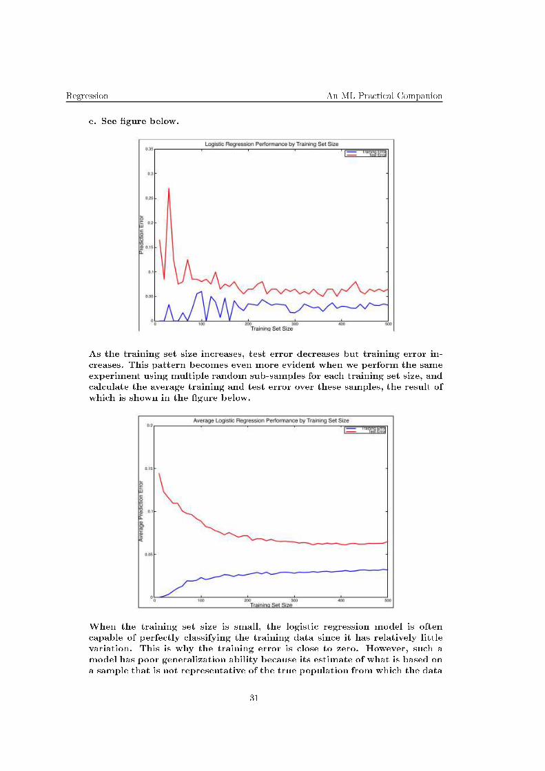
e. See gure below.
As the training set size in reases, test error de reases but training error in-
reases. This pattern be omes even more evident when we perform the same
experiment using multiple random sub-samples for ea h training set size, and
al ulate the average training and test error over these samples, the result of
whi h is shown in the gure below.
When the training set size is small, the logisti regression model is often
apable of perfe tly lassifying the training data sin e it has relatively little
variation. This is why the training error is lose to zero. However, su h a
model has poor generalization ability be ause its estimate of what is based on
a sample that is not representative of the true population from whi h the data
31
An ML Pra ti al Companion Regression
is drawn. This phenomenon is known as overtting be ause the model ts too
losely to the training data. As the training set size in reases, more variation
is introdu ed into the training data, and the model is usually no longer able
to t to the training set as well. This is also due to the fa t that the omplete
dataset is not 100% linearly separable. At the same time, more training data
provides the model with a more omplete pi ture of the overall population,
whi h allows it to learn a more a urate estimate of wHat. This in turn leads
to better generalization ability i.e. lower predi tion error on the test dataset.
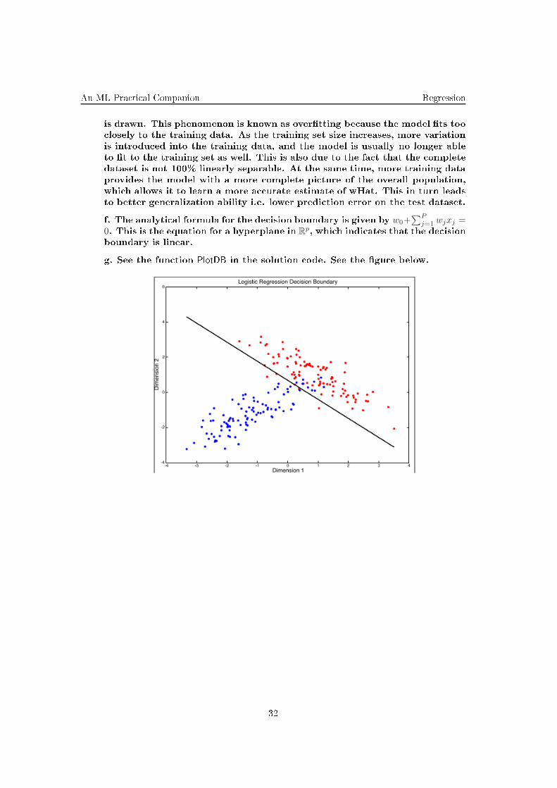
f. The analyti al formula for the de ision boundary is given by w0+∑P
j=1 wjxj =0. This is the equation for a hyperplane in R
p, whi h indi ates that the de ision
boundary is linear.
g. See the fun tion PlotDB in the solution ode. See the gure below.
32

Regression An ML Pra ti al Companion
12. (Logisti Regression (with gradient as ent)
xxx and Rosenblatt's Per eptron:
xxx appli ation on the Breast Can er dataset
xxx n-fold ross-validation; onden e interval)
• (CMU, 2009 spring, Ziv Bar-Joseph, HW2, pr. 4)
For this exer ise, you will use the Breast Can er dataset, downloadable from
the ourse web page. Given 9 dierent attributes, su h as uniformity of ell
size, the task is to predi t malignan y.
701
The ar hive from the ourse web
page ontains a Matlab method loaddata.m, so you an easily load in the data
by typing (from the dire tory ontaining loaddata.m): data = loaddata. The
variables in the resulting data stru ture relevant for you are:
• data.X: 683 9-dimensional data points, ea h element in the interval [1, 10].
• data.Y: the 683 orresponding lasses, either 0 (benign), or 1 (malignant).
Logisti Regression
a. Write ode in Matlab to train the weights for logisti regression. To avoid
dealing with the inter ept term expli itly, you an add a nonzero- onstant
tenth dimension to data.X: data.X(:,10)=1. Your regression fun tion thus be-
omes simply:
P (Y = 0|x;w) =1
1 + exp(∑10
k=1 xkwk)
P (Y = 1|x;w) =exp(
∑10k=1 xkwk)
1 + exp(∑10
k=1 xkwk)
and the gradient-as end update rule:
w← w + α/683
683∑
j=1
xj(yj − P (Y j = 1|xj ;w))
Use the learning rate α = 1/10. Try dierent learning rates if you annot get
w to onverge.
b. To test your program, use 10-fold ross-validation, splitting [data.X data.Y
into 10 random approximately equal-sized portions, training on 9 on atenated
parts, and testing on the remaining part. Report the mean lassi ation
a ura y over the 10 runs, and the 95% onden e interval.
Rosenblatt's Per eptron
A very simple and popular linear lassier is the per eptron algorithm of
Rosenblatt (1962), a single-layer neural network model of the form
y(x) = f(w⊤x),
with the a tivation fun tion
f(a) =
1 if a ≥ 0−1 otherwise.
701
For more information on what the individual attributes mean, see ftp://ftp.i s.u i.edu/pub/ma hine-
learning-databases/breast- an er-wis onsin/breast an er-wis onsin.names.
33
An ML Pra ti al Companion Regression
For this lassier, we need our lasses to be −1 (benign) and 1 (malignant),
whi h an be a hieved with the Matlab ommand: data.Y = data.Y ⋆ 2 - 1.
Weight training usually pro eeds in an online fashion, iterating through the
individual data points xjone or more times. For ea h xj
, we ompute the
predi ted lass yj = f(w⊤xj) for xjunder the urrent parameters w, and update
the weight ve tor as follows:
w ← w + xj [yj − yj ].
Note how w only hanges if xj was mis lassied under the urrent model.
. Implement this training algorithm in Matlab. To avoid dealing with the in-
ter ept term expli itly, augment ea h point in data.X with a non-zero onstant
tenth element. In Matlab this an be done by typing: data.X(:,10)=1. Have
your algorithm iterate through the whole training data 20 times and report the
number of examples that were still mis- lassied in the 20th iteration. Does
it look like the training data is linearly separable? (Hint: The per eptron
algorithm is guaranteed to onverge if the data is linearly separable.)
d. To test your program, use 10-fold ross-validation, using the splits you
obtained in part b. For ea h split, do 20 training iterations to train the wei-
ghts. Report the mean lassi ation a ura y over the 10 runs, and the 95%
onden e interval.
e. If the data is not linearly separable, weights an toggle ba k and forth
from iteration to iteration. Even in the linearly separable ase, the learned
model is often very dependent on whi h training data points ome rst in the
training sequen e. A simple improvement is the weighted per eptron: training
pro eeds as before, but the weight ve tor w is saved after ea h update. After
training, instead of the nal w, the average of all saved w is taken to be
the learned weight ve tor. Report 10-fold CV a ura y for this variant and
ompare it to the simple per eptron's.
Solution:
You should have gotten something like this:
b. mean a ura y: 0.965, onden e interval: (0.951217, 0.978783).
. 30 mis- lassi ations in the 20th iteration. (Note that using the trained
weights *after* the 20th iteration results in only around 24 mis- lassi ations.)
When running with 200 iterations, still more than 20 mis- lassi ations o ur,
so the data is unlikely to be linearly separable as otherwise the training error
would be ome zero after many enough iterations.
d. Per eptron:
mean a ura y = 0.956, 95% onden e interval: (0.940618, 0.971382).
e. Weighted per eptron:
mean a ura y = 0.968, 95% onden e interval: (0.954800, 0.981200).
34

Regression An ML Pra ti al Companion
13. (Logisti regression using Newton's method:
xxx appli ation on R2data)
• Stanford, 2011 fall, Andrew Ng, HW1, pr. 1.b
a. On the web page asso iated to this booklet, you will nd the les q1x.dat
and q1y.dat whi h ontain the inputs (x(i) ∈ R2) and outputs (y(i) ∈ 0, 1) res-
pe tively for a binary lassi ation problem, with one training example per
row.
Implement Newton's method for optimizing ℓ(θ), the [ onditional] log-likelihoodfun tion
ℓ(θ) =
m∑
i=1
y(i) lnσ(w · x(i)) + (1 − y(i)) ln(1− σ(w · x(i))),
and apply it to t a logisti regression model to the data. Initialize Newton's
method with θ = 0 (the ve tor of all zeros). What are the oe ients θresulting from your t? (Remember to in lude the inter ept term.)
b. Plot the training data (your axes should be x1 and x2, orresponding to the
two oordinates of the inputs, and you should use a dierent symbol for ea h
point plotted to indi ate whether that example had label 1 or 0). Also plot
on the same gure the de ision boundary t by logisti regression. (I.e., this
should be a straight line showing the boundary separating the region where
h(x) > 0.5 from where h(x) ≤ 0.5.)
Solution:
a. θ = (−2.6205, 0.7604, 1.1719)with the rst entry orresponding to the inter eptterm.
b.
35

An ML Pra ti al Companion Regression
14. (Solving logisti regression, the kernelized version,
xxx using Newton's method:
xxx implementation + appli ation on R2data)
• CMU, 2005 fall, Tom Mit hell, HW3, pr. 2. d
a. Implement the kernel logisti regression des ribed in ex. 15 in our exer ise
book, using the gaussian kernel Kσ(x, x′) = exp
(‖x− x′‖22σ2
)
.
Run your program on the le ds2.txt (the rst two olumns are X, the last
olumn is Y ) with σ = 1. Report the training error. Set stepsize to be 0.01and the maximum number of iterations 100. The s atterplot of the ds2.txt data
is the follows:
b. Use 10-fold ross-validation to nd the best σ and plot the total number
of mistakes for σ ∈ 0.5, 1, 2, 3, 4, 5, 6.
Solution:
a. 53 mis lassi ations.
b. The best value of σ is 2.
36

Regression An ML Pra ti al Companion
15. (Lo ally-weighted, regularized (L2) logisti regression,
xxx using Newton's method:
xxx appli ation on dataset from R2)
• Stanford, 2007 fall, Andrew Ng, HW1, pr. 2
In this problem you will implement a lo ally-weighted version of logisti re-
gression whi h was des ribed in the 31 exer ise in the Estimating the para-
meters of some probabilisti distributions hapter of our exer ise book. For
the entirety of this problem you an use the value λ = 0.0001.
Given a query point x, we hoose ompute the weights
wi = exp
(
−‖x− xi‖22τ2
)
.
This s heme gives more weight to the nearby points when predi ting the
lass of a new example[, mu h like the lo ally weighted linear regression dis-
ussed at exer ise ??.
a. Implement the Newton algorithm for optimizing the log-likelihood fun tion
(ℓ(θ) in the 31 exer ise) for a new query point x, and use this to predi t the
lass of x. The q2/ dire tory ontains data and ode for this problem. You
should implement the y = lwlr(X_train, y_train, x, tau) fun tion in the lwlr.m
le. This fun tion takes as input the training set (the X_train and y_train
matri es), a new query point x and the weight bandwitdh tau. Given this
input, the fun tion should i . ompute weights wi for ea h training example,
using the formula above, ii . maximize ℓ(θ) using Newton's method, and iii .
output y = 1hθ(x)>0.5 as the predi tion.
We provide two additional fun tions that might help. The [X_train, y_train =
load_data; fun tion will load the matri es from les in the data/ folder. The
fun tion plot_lwlr(X_train, y_train, tau, resolution) will plot the resulting lassier
(assuming you have properly implemented lwlr.m). This fun tion evaluates the
lo ally weighted logisti regression lassier over a large grid of points and
plots the resulting predi tion as blue (predi ting y = 0) or red (predi ting
y = 1). Depending on how fast your lwlr fun tion is, reating the plot might
take some time, so we re ommend debugging your ode with resolution = 50; and
later in rease it to at least 200 to get a better idea of the de ision boundary.
b. Evaluate the system with a variety of dierent bandwidth parameters τ .In parti ular, try τ = 0.01, 0.05, 0.1, 0.5, 1.0, 5.0. How does the lassi ation
boundary hange when varying this parameter? Can you predi t what the
de ision boundary of ordinary (unweighted) logisti regression would look
like?
Solution:
a. Our implementation of lwlr.m:
fun tion y = lwlr(X_train, y_train, x, tau)
m = size(X_train, 1);
n = size(X_train, 2);
theta = zeros(n, 1);
% ompute weights
37

An ML Pra ti al Companion Regression
w = exp(-sum((X_train - repmat(x', m, 1)).
∧2, 2) / (2*tau));
% perform Newton's method
g = ones(n, 1);
while (norm(g) > 1e-6)
h = 1 ./ (1 + exp(-X_train * theta));
g = X_train' * (w.*(y_train - h)) - 1e-4*theta;
H = -X_train' * diag(w.*h.*(1-h)) * X_train - 1e-4*eye(n);
theta = theta - H g;
end
% return predi ted y
y = double(x'*theta > 0);
b. These are the resulting de ision boundaries, for the dierent values of τ :
For smaller τ , the lassier appears to overt the data set, obtaining zero trai-ning error, but outputting a sporadi looking de ision boundary. As τ grows,the resulting de ision boundary be omes smoother, eventually onverging (in
the limit as τ →∞ to the unweighted linear regression solution).
38

Regression An ML Pra ti al Companion
16. (Logisti regression with L2 regularization;
xxx appli ation on handwritten digit re ognition;
xxx omparison between the gradient method and Newton's method)
• MIT, 2001 fall, Tommi Jaakkola, HW2, pr. 4
Here you will solve a digit lassi ation problem with logisti regression mo-
dels. We have made available the following training and test sets: digit_x.dat,
digit_y.dat, digit_x_test.dat, digit_y_test.dat.
a. Derive the sto hasti gradient as ent learning rule for a logisti regression
model starting from the regularized likelihood obje tive
J(w; c) = . . .
where ‖w‖2 =∑d
i=0 w2i [or by modifying your derivation of the delta rule for
the softmax model. (Normally we would not in lude w0 in the regularization
penalty but have done so here for simpli ity of the resulting update rule).
b. Write a MATLAB fun tion w = SGlogisti reg(X,y, ,epsilon) that takes inputs si-
milar to logisti reg from the previous se tion, and a learning rate parameter
ε, and uses sto hasti gradient as ent to learn the weights. You may in lude
additional parameters to ontrol when to stop, or hard- ode it into the fun -
tion.
. Provide a rationale for setting the learning rate and the stopping riterion
in the ontext of the digit lassi ation task. You should assume that the
regularization parameter remains xed at 1. (You might wish to experiment
with dierent learning rates and stopping riterion but do NOT use the test
set. Your justi ation should be based on the available information before
seeing the test set.)
d. Set c = 1 and apply your pro edure for setting the learning rate and the
stopping riterion to evaluate the average log-probability of labels in the trai-
ning and test sets. Compare the results to those obtained with logisti reg. For
ea h optimization method, report the average log-probabilities for the labels
in the training and test sets as well as the orresponding mean lassi ation
errors (estimates of the miss- lassi ation probabilities). (Please in lude all
MATLAB ode you used for these al ulations.)
e. Are the train/test dieren es between the optimization methods reasona-
ble? Why? (Repeat the gradient as ent pro edure a ouple of times to ensure
that you are indeed looking at a typi al out ome.)
f. The lassiers we found above are both linear lassiers, as are all logisti
regression lassiers. In fa t, if we set c to a dierent value, we are still
sear hing the same set of linear lassiers. Try using logisti reg with dierent
values of c, to see that you get dierent lassi ations. Why are the resulting
lassiers dierent, even though the same set of lassiers is being sear hed?
Contrast the reason with the reason for the dieren es you explained in the
previous question.
g. Gaussian mixture models with identi al ovarian e matri es also lead to
linear lassiers. Is there a value of c su h that training a Gaussian mix-
ture model ne essarily leads to the same lassi ation as training a logisti
regression model using this value of c? Why?
39

An ML Pra ti al Companion Regression
Solution:
a.
w ←(
1− ε c
n
)
w + ε(yi − P (1|xi, w))xi.
[LC: You an nd the details in the MIT do ument.]
b.
fun tion [w = SGlogisti reg(X,y, ,epsilon,stopdelta)
[n,d = size(X);
X = [ones(n,1),X;
w = zeros(d+1,1);
ont = 1;
while ( ont)
perm = randperm(n);
oldw = w;
for i = 1:n
w = (1 - epsilon * / n) * w + epsilon * (y(i) - g(X(i,:) * w)) * X(i,:)' ;
end
ont = norm(oldw - w) >= stopdelta * norm(oldw) ;
end
. Learning rate: If the learning rate is too high, any memory of previous
updates will be wiped out (beyond the last few points used in the updates).
It's important that all the points ae t the resulting weights and so the lear-
ning rate should s ale somehow with the number of examples. But how?
When the sto hasti gradient updates onverge, we are not hanging the wei-
ghts on average. So ea h update an be seen as a slight random perturbation
around the orre t weights. We'd like to keep su h sto hasti ee ts from
pushing the weights too far from the optimal solution. One way to deal with
this is to simply average the random ee ts by making the learning rate s ale
as ε =c
nfor a onstant c, somewhat less than one.
But this would be slow. It's good to keep the varian e of the sum of the
random perturbation at a onstant and instead set ε =c√n: You may re all
that if Zi is a Gaussian with zero zero and unit varian e, then
∑
i = 1nZi
has varian e n. Here Zi orresponds to a gradient update based on the i-th example. Dividing by the standard deviation of the sum,
√n, makes the
gradient updates have an overall xed varian e.
Sin e the update is also proportional to the norm of the input examples you
might also divide the learning rate by the overall s ale of the inputs. If we
have d binary oordinates, the norm is at most d. We get a learning rate of
ε =c√n d
.
Stopping riterion: We want to stop when a full iteration through the training
set does not make mu h dieren e on average. Note that unless we an
perfe tly separate the training set, we would still expe t to get spe i training
examples that will ause hange, but at onvergen e they should an el ea h
other out. We should also not stop just be ause one, or a few, examples did
not ause mu h hange - it might be that other examples will.
And so, after ea h full iteration through the training set, we see how mu h
the weight hanged sin e before the iteration. As we do not know what the
40

Regression An ML Pra ti al Companion
Figura 1: Logisti regression log-likelihood, when trained with sto hasti gradient as ent, for
varying stopping riteria.
s ale of the weights will be, we he k the magnitude of the hange relative to
the magnitude of the weights. We stop if the hange falls bellow some low
threshold, whi h represents out desired a ura y of the result (this ratio is
the parameter stopdelta).
d. To al ulate also the lassi ation errors, we use a slightly expanded version
of logisti ll.m:
fun tion [ll,err = logisti le(x,y,w)
p = g(w(1) + x*w(2:end));
ll = mean(y.*log(p) + (1-y).*log(1-p));
err = mean(y ˜= (p > 0.5));
We set the learning rate to: ε =0.1√n d
=0.1
80, try a stopping granularity of
δ = 0.0001, and get:
Average log-probabilities:
Sto hasti
Newton-Raphson Gradient As ent
Train -0.0829 -0.1190
test -0.2876 -0.2871
Classi ation errors:
Sto hasti
Newton-Raphson Gradient As ent
Train 0.01 0.02
test 0.125 0.1125
Results for various stopping granularities are presented in gures 1 and 2.
e. Although both optimization methods are trying to optimize the same
obje tive fun tion, neither of them is perfe t, and so we expe t to see some
dis repan ies, as we do in fa t see.
41
An ML Pra ti al Companion Regression
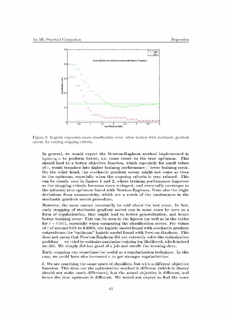
Figura 2: Logisti regression mean lassi ation error, when trained with sto hasti gradient
as ent, for varying stopping riteria.
In general, we would expe t the Newton-Raphson method implemented in
logisti reg.m to perform better, i.e. ome loser to the true optimum. This
should lead to a better obje tive fun tion, whi h espe ially for small values
of c, would translate into higher training performan e / lower training error.
On the other hand, the sto hasti gradient as ent might not ome as lose
to the optimum, espe ially when the stopping riteria is very relaxed. This
an be learly seen in gures 1 and 2, where training performan e improves
as the stopping riteria be omes more stringent, and eventually onverges to
the (almost) true optimum found with Newton-Raphson. Note also the slight
deviations from monotoni ity, whi h are a result of the randomness in the
sto hasti gradient as ent pro edure.
However, the same annot ne essarily be said about the test error. In fa t,
early stopping of sto hasti gradient as ent an in some ases be seen as a
form of regularization, that might lead to better generalization, and hen e
better training error. This an be seen in the gures (as well as in the tables
for δ = 0.001), espe ially when omparing the lassi ation errors. For values
of δ of around 0.01 to 0.0005, the logisti model found with sto hasti gradient
outperforms the optimum logisti model found with Newton-Raphson. This
does not mean that Newton-Raphson did not orre tly solve the optimization
problemwe tried to optimize maximize training log likelihood, whi h indeed
we did. We simply did too good of a job and overt the training data.
Early stopping an sometimes be useful as a regularization te hnique. In this
ase, we ould have also in reased to get stronger regularization.
f. We are sear hing the same spa e of lassiers, but with a dierent obje tive
fun tion. This time not the optimization method is dierent (whi h in theory
should not make mu h dieren e), but the a tual obje tive is dierent, and
hen e the true optimum is dierent. We would not expe t to nd the same
42

Regression An ML Pra ti al Companion
lassier.
g. There is no su h value of c. The obje tive fun tions are dierent, even
for c = 0. The logisti regression obje tive fun tion aims to maximize the
likelihood of the labels given the input ve tors, while the Gaussian mixture
obje tive is to t a probabilisti model for the training input ve tors and
labels, by maximizing their joint joint likelihood.
43
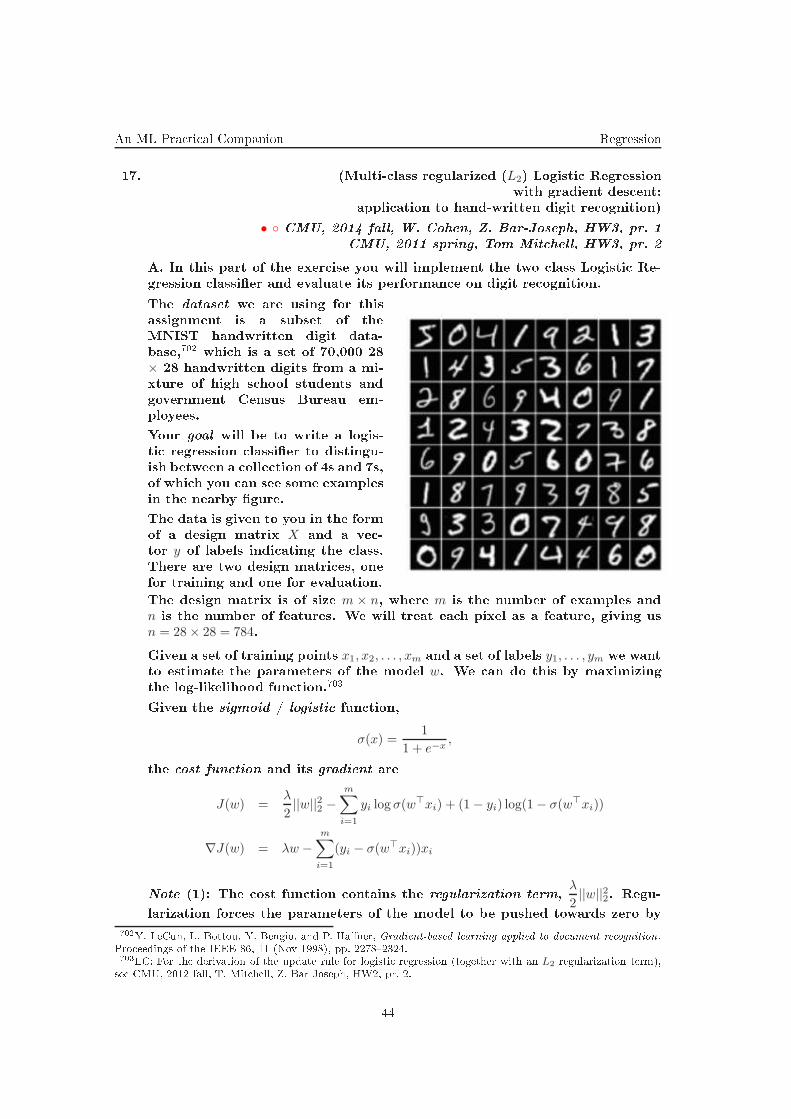
An ML Pra ti al Companion Regression
17. (Multi- lass regularized (L2) Logisti Regression
xxx with gradient des ent:
xxx appli ation to hand-written digit re ognition)
• CMU, 2014 fall, W. Cohen, Z. Bar-Joseph, HW3, pr. 1
xxx CMU, 2011 spring, Tom Mit hell, HW3, pr. 2
A. In this part of the exer ise you will implement the two lass Logisti Re-
gression lassier and evaluate its performan e on digit re ognition.
The dataset we are using for this
assignment is a subset of the
MNIST handwritten digit data-
base,
702
whi h is a set of 70,000 28
× 28 handwritten digits from a mi-
xture of high s hool students and
government Census Bureau em-
ployees.
Your goal will be to write a logis-
ti regression lassier to distingu-
ish between a olle tion of 4s and 7s,
of whi h you an see some examples
in the nearby gure.
The data is given to you in the form
of a design matrix X and a ve -
tor y of labels indi ating the lass.
There are two design matri es, one
for training and one for evaluation.
The design matrix is of size m × n, where m is the number of examples and
n is the number of features. We will treat ea h pixel as a feature, giving us
n = 28× 28 = 784.
Given a set of training points x1, x2, . . . , xm and a set of labels y1, . . . , ym we want
to estimate the parameters of the model w. We an do this by maximizing
the log-likelihood fun tion.
703
Given the sigmoid / logisti fun tion,
σ(x) =1
1 + e−x,
the ost fun tion and its gradient are
J(w) =λ
2||w||22 −
m∑
i=1
yi log σ(w⊤xi) + (1− yi) log(1− σ(w⊤xi))
∇J(w) = λw −m∑
i=1
(yi − σ(w⊤xi))xi
Note (1): The ost fun tion ontains the regularization term,
λ
2||w||22. Regu-
larization for es the parameters of the model to be pushed towards zero by
702
Y. LeCun, L. Bottou, Y. Bengio, and P. Haner, Gradient-based learning applied to do ument re ognition.
Pro eedings of the IEEE 86, 11 (Nov 1998), pp. 22782324.
703
LC: For the derivation of the update rule for logisti regression (together with an L2 regularization term),
see CMU, 2012 fall, T. Mit hell, Z. Bar-Joseph, HW2, pr. 2.
44

Regression An ML Pra ti al Companion
Tabela 1: Summary of notation used for Logisti Regression
Not. Meaning Type
m number of training examples s alar
n number of features s alar
xi ith augmented training data point (one digit example) (n+ 1)× 1X design matrix (all training examples) m× (n+ 1)yi ith training label (is the digit a 7?) 0, 1
Y or y all training labels m× 1w parameter ve tor (n+ 1)× 1S sigmoid fun tion, S(t) = (1 + e−t)−1
dim(t) → dim(t)J ost (loss) fun tion R
n → R
∇J gradient of J (ve tor of derivatives in ea h dimension) Rn → R
n
α (parameter) gradient des ent learning rate s alar
d (parameter) de ay onstant for α to de rease s alar
by every iteration
λ (parameter) regularization strength s alar
penalizing large w values. This helps to prevent overtting and also makes
the obje tive fun tion stri tly on ave, whi h means that there is a unique
solution.
Note (2): Please regularize the inter ept term too, i.e., w(0)should also be
regularized.
704
In order to keep the notation lean and make the implemen-
tation easier, we assume that ea h xi has been augmented with an extra 1 atthe beginning, i.e., x′
i = [1;xi]. Therefore our model of the log-odds is
log1− p
p= w(0) + w(1)x(1) + . . .+ w(n)x(n).
Note (3): For models su h as linear regression we were able to nd a lo-
sed form solution for the parameters of the model. Unfortunately, for many
ma hine learning models, in luding Logisti Regression, no su h losed form
solutions exist. Therefore we will use a gradient-based method to nd our
parameters.
The update rule for gradient as ent is
wi+1 = wi + αdi∇J(wi),
where α spe ies the learning rate, or how large a step we wish to take, and dis a de ay term that we use to ensure that the step sizes we make will gradually
get smaller, so long as we onverge. The iteration stops when the hange of xor f(x) is smaller than a threshold.
a. Implement the ost fun tion and the gradient for logisti regression in
ostLR.m.
705
Implement gradient des ent in minimize.m. Use your minimizer
to omplete trainLR.m.
704
Many resour es about Logisti Regression on the web do not regularize the inter ept term, so be aware if
you see dierent obje tive fun tions.
705
You an run run_logit.m to he k whether your gradients mat h the ost. The s ript should pass the
gradient he ker and then stop.
45
An ML Pra ti al Companion Regression
b. On e you have trained the model, you an then use it to make predi tions.
Implement predi tLR, whi h will generate the most likely lasses for a given
xi.
B. In this part of the exer ise you will implement the multi- lass lass Logisti
Regression lassier and evaluate its performan e on another digit re ognition,
provided by USPS. In this dataset, ea h hand-written digital image is 16 by
16 pixels. If we treat the value of ea h pixel as a boolean feature (either 0
for bla k or 1 for white), then ea h example has 16 × 16 = 256 0, 1-valuedfeatures, and hen e x has 256 dimension. Ea h digit (i.e., 1,2,3,4,5,6,7,8,9,0)
orresponds to a lass label y (y = 1, . . . ,K, K = 10). For ea h digit, we have
600 training samples and 500 testing samples.
706
Please download the data from the website. Load the usps digital.mat le in
usps_digital.zip into Matlab. You will have four matri es:
• tr_X: training input matrix with the dimension 6000× 256.
• tr_y: training label of the length 6000, ea h element is from 1 to 10.
• te_X: testing input matrix with the dimension 5000× 256.
• te_y: testing label of the length 5000, ea h element is from 1 to 10.
For those who do NOT want to use Matlab, we also provide the text le
for these four matri es in usps_digital.zip. Note that if you want to view
the image of a parti ular training/testing example in Matlab, say the 1000th
training example, you may use the following Matlab ommand:
imshow(reshape(tr_X(1000,:),16,16)).
. Use the gradient as ent algorithm to train a multi- lass logisti regression
lassier. Plot (1) the obje tive value (log-likelihood), (2) the training a u-
ra y, and (3) the testing a ura y versus the number of iterations. Report
your nal testing a ura y, i.e., the fra tion of test images that are orre tly
lassied.
Note that you must hoose a suitable learning rate (i.e. stepsize) of the
gradient as ent algorithm. A hint is that your learning rate annot be too
large otherwise your obje tive will in rease only for the rst few iterations.
In addition, you need to hoose a suitable stopping riterion. You might use
the number of iterations, the de rease of the obje tive value, or the maxi-
mum of the L2 norms of the gradient with respe t to ea h wk. Or you might
wat h the in rease of the testing a ura y and stop the optimization when the
a ura y is stable.
d. Now we add the regularization term
λ
2
∑K−1i=1 ||wl||22. For λ = 1, 10, 100, 1000,
report the nal testing a ura ies.
e. What an you on lude from the above experiment? (Hint: the relationship
between the regularization weight and the predi tion performan e.)
Solution:
b. You should get about 96% a ura y.
706
You an view these images at http://www. s.nyu.edu/∼roweis/data/usps_0.jpg, . . . ,
http://www. s.nyu.edu/∼roweis/data/usps_9.jpg.
46

Regression An ML Pra ti al Companion
. I use the stepsize η = 0.0001 and run the gradient as ent method for 5000
iterations. The obje tive value vs. the number of iterations, training error
vs. the number of iterations, testing error vs. the number of iterations are
presented in gure below:
d. For λ = 0, 1, 10, 100, 1000, the omparison of the testing a ura y is presented
in the next table:
λ 0 1 10 100 1000Testing a ura y 91.44% 91.58% 91.92% 89.74% 79.78%
e. From the above result, we an see that adding the regularization ould
avoid overtting and lead to better generalization performan e (e.g., λ = 1, 10).However, the regularization annot be too large. Although a larger regulari-
zation an de rease the varian e, it introdu es additional bias and may lead
to worse generalization performan e.
47

An ML Pra ti al Companion Regression
18. (Multinomial/Categori al Logisti Regression,
xxx Gaussian Naive Bayes, Gaussian Joint Bayes, and k-NN:xxx appli ation on the ORL Fa es dataset)
• · CMU 2010 spring, E. Xing, T. Mit hell, A. Singh, HW2, pr. 2
In this part, you are going to play with The ORL Database of Fa es.
6 sample images from two persons
Ea h image is 92 by 112 pixels. If we treat the luminan e of ea h pixel as
a feature, ea h sample has 92 ∗ 112 = 10304 real value features, whi h an
be written as a random ve tor X. We will treat ea h person as a lass Y(Y = 1, . . . ,K, K = 10). We use Xi to refer the i-th feature. Given a set
of training data D = (yl, xl), we will train dierent lassi ation models to
lassify images to their person id's. To simplify notation, we will use P (y|x)in pla e of P (Y = y|X = x).
We will sele t our models by 10-fold ross validation: partition the data for
ea h fa e into 10 mutually ex lusive sets (folds). In our ase, exa tly one
image for ea h fold. Then, for k = 1, . . . , 10, leave out the data from fold k for
all fa es, train on the rest, and test on the left out data. Average the results
of these 10 tests to estimate the training a ura y of your lassier.
Note: Beware that we are a tually not evaluating the generalization errors of
the lassier here. When evaluating generalization error, we would need an
independent test set that is not at all tou hed during the whole developing
and tuning pro ess.
For your onvenien e, a pie e of ode loadFa es.m is provided to help loading
images as feature ve tors.
From Tom Mit hell's additional book hapter,
707
page 13, you will see a gene-
ralization of logisti regression, whi h allows Y to have more than two possible
values.
a. Write down the obje tive fun tion, and the rst order derivatives of the
multinomial logisti regression model (whi h is a binary lassier).
708
Here we will onsider a L2-norm regularized obje tive fun tion (with a term
λ|θ|2).
b. Implement the logisti regression model with gradient as ent. Show your
evaluation result here. Use regularization parameter λ = 0.
707
www. s. mu.edu/∼tom/mlbook/NBayesLogReg.pdf.
708
Hint: In order to do k- lass lassi ation with binary lassier, we use a voting s heme. At training time,
a lassier is trained for any pair of lasses. At testing time, all k(k − 1)/2 lassiers are applied to the testing
sample. Ea h lassier either vote for its rst lass or its se ond lass. The lass voted by most number of
lassiers is hosen as the predi tion.
48
Regression An ML Pra ti al Companion
Hint: The gradient as ent method (also known as steepest as ent) is a rst-
order optimization algorithm. It optimizes a fun tion f(x) by
xt+1 = xt + αtf′(xt),
where αt is alled the step size, whi h is often pi ked by line sear h. For
example, we an initialize αt = 1.0. Then set αt = αt/2 while f(xt + αtf′(xt)) <
f(xt). The iteration stops when the hange of x or f(x) is smaller than a
threshold.
Hint: If the training time of your model is too long, you an onsider use just
a subset of the features (e.g., in Matlab X = X(:,1:100:d)).
. Overtting and Regularization
Now we test how regularization an help prevent overtting. During ross-
validation, let's use m images from ea h person for training, and the rest
for testing. Report your ross-validated result with varying m = 1, . . . , 9 and
varying regularization parameter λ.
d. Logisti Regression and Newton's method
Newton's method (also known as the Newton-Raphson method) is a rst-
order optimization algorithm, whi h often onverges in a few iterations. It
Optimize a fun tion f(x) by the update equation
xt+1 = xt −f ′(xt)
f ′′(xt)
The iteration stops when the hange of x or f(x) is smaller than a threshold.
Write down the se ond order derivatives and the update equation of the lo-
gisti regression model.
Implement the logisti regression model with Newton's method. Show your
evaluation result here.
B. Implement the k-NN algorithm. Use L2-norm as the distan e metri . Show
your evaluation result here, and ompare dierent values of k.
C. Conditional Gaussian Estimation
For a Gaussian model we have
P (y|x) = P (x|y)P (y)
P (x),
where
P (x|y) = 1
(2π)d/2|Σy|1/2exp(−(x − µy)
⊤Σ−1(x− µy)/2),
and P (y) = πy. Please write down the MLE estimation of model parameters
Σy, µy, and πy. Here we do not assume that Xi are independent given Y .
D. Gaussian Naive Bayes is a form of Guassian model with assumption that
Xi are independent given Y . Implement the Gaussian NB model, and briey
des ribe your evaluation result.
E. Compare the above methods by training/testing time, and a ura y.
Whi h method do you prefer?
49

An ML Pra ti al Companion Regression
19. (Model sele tion:
xxx sentiment analysis for musi reviews
xxx using a dataset provided by Amazon,
xxx using lasso logisti regression)
• · CMU, 2014 spring, B. Po zos, A. Singh, HW2, pr. 5
In this homework, you will perform model sele tion on a sentiment analysis
dataset of musi reviews.
709
The dataset onsists of reviews from Amazon. om
for musi s. The ratings have been onverted to a binary label, indi ating a
negative review or a positive review. We will use lasso logisti regression for
this problem.
710
The lasso logisti regression obje tive fun tion to minimize
during training is:
L(β) = log(1 + exp(−yβ⊤x)) + λ‖β‖1
In lasso logisti regression, we penalize the loss fun tion by an L1 norm of
the feature oe ients. Penalization with an L1 norm tends to produ e so-
lutions where some oe ients are exa tly 0. This makes it attra tive for
high-dimensional data su h as text, be ause in most ases most words an
typi ally be ignored. Furthermore, sin e we are often left with only a few
nonzero oe ients, the lasso solution is often easy to interpret.
The goal of model sele tion here is to hoose λ sin e ea h setting of λ implies
a dierent model size (number of non-zero oe ients).
You do not need to implement lasso logisti regression. You an download
an implementation from https://github. om/redpony/ reg, and the dataset an be
found on the ourse web page. There are three feature les and three response
(label) les (all response les end with .res). They are already in the format
required by the implementation you will use. The les are:
• Training data: musi .train and musi .train.res
• Development data: musi .dev and musi .dev.res
• Test data: musi .test and musi .test.res
Important note: The ode outputs a ura y , whereas you need to plot las-
si ation error here. You an simply transform a ura y to error by using
1− a ura y.
Error on development (validation) data
In the rst part of the problem, we will use error on a development data to
hoose λ. Run the model with λ = 10−8, 10−7, 10−6, . . . , 10−1, 1, 10, 100.a. Plot the error on training data and development data as a fun tion of logλ.
b. Plot the model size (number of nonzero oe ients) on development data
as a fun tion of logλ.
. Choose λ that gives the lowest error on development data. Run it on the
test data and report the test error.
709
John Blitzer, Mark Dredze, and Fernando Pereira. Biographies, Bollywood, Boom-boxes and Blenders:
Domain Adaptation for Sentiment Classi ation. In Pro eedings of ACL, 2007.
710
Robert Tibshirani. Regression shrinkage and sele tion via the lasso, In Journal of Royal Statisti al So iety
B, 58(1):267:288, 1996.
50

Regression An ML Pra ti al Companion
Briey dis uss all the results.
Model Complexity and Bias-Varian e Tradeo
d. Give a high-level explanation on the relation between λ and the bias and
varian e of parameter estimates β. Does larger λ orrespond to higher or
lower bias? What about the varian e? Does larger λ lead to a more omplex
or a less omplex model?
Resolving a tie
e. If there are more than one λ that minimizes the error on the development
data, whi h one will you pi k? Explain your hoi e.
Random sear h
f. An alternative way to sear h λ is by randomly sampling its value from an
interval.
i. Sample eleven random values log uniformly from an interval [10−8, 100] forλ and train a lasso logisti regression model. Plot the error on develop-
ment data as a fun tion of logλ.
ii. Choose λ that gives the lowest error on development data. Run it on the
test data and report the test error.
Random vs. grid sear h
g. Whi h one do you think is a better method for sear hing values to try for
λ? Why?
51

An ML Pra ti al Companion Regression
20. (Metoda [sub-gradientului:
x diferite fun µii de ost / pierdere ³i
x diferite fun µii / metode de regularizare)
• CMU, 2015 spring. Alex Smola, HW8, pr. 1
52
Bayesian Classi ation An ML Pra ti al Companion
2 Bayesian Classi ation
21. (Naive Bayes: weather predi tion;
xxx feature sele tion based on CVLOO)
• CMU, 2010 fall, Ziv Bar-Joseph, HW1, pr. 4
xxx CMU, 2009 fall, Ziv Bar-Joseph, HW1, pr. 3
You need to de ide whether to arry an umbrella to s hool in Pittsburgh as
the lo al weather hannel has been giving in onsistent predi tions re ently.
You are given several input features (observations). These observations are
dis rete, and you are expe ted to use a Naive Bayes lassi ation s heme to
de ide whether or not you will take your umbrella to s hool. The domain of
ea h of the features is as follows:
season = (w, sp, su, f)
yesterday = (dry, rainy)
daybeforeyesterday = (dry, rainy)
loud = (sunny, loudy)
and the possible lasses of the output being: umbrella = (y, n).
See data1.txt (posted on website with problem set) for data based on the
above s enario with spa e separated elds onforming to:
season yesterday daybeforeyesterday loud umbrella
a. Write ode in MATLAB to estimate the onditional probabilities of ea h
the features given the out ome. Generate a spa e separated le with the
estimated parameters from the entire dataset by writing out all the onditional
probabilities.
b. Write ode in MATLAB to perform inferen e by predi ting the maximum
likelihood lass based on training data using a leave one out ross validation
s heme. Generate a [spa e separated le with the maximum likelihood lasses
in order.
. Are the features yesterday and daybeforeyesterday independent of ea h
other?
d. Does the Naive Bayes assumption hold on this pair of input features? Why
or why not?
e. Find a subset of 3 features from this set of 4 features where your algorithm
improves its predi tive ability based on a leave one out ross validation s heme.
Report your improvement.
Solution:
a. Without pseudo ounts, the onditional probabilities are:
loud loudy y 0.8
loud sunny y 0.2
loud sunny n 0.6
loud loudy n 0.4
daybeforeyesterday dry y
53

An ML Pra ti al Companion Bayesian Classi ation
daybeforeyesterday rainy
daybeforeyesterday dry n
daybeforeyesterday rainy
season w n 0.3
season sp n 0
season su n 0.3
season f n 0.4
season sp y 0.2
season su y 0.1
season f y 0.4
season w y 0.3
yesterday dry y 0.4
yesterday rainy y 0.6
yesterday rainy n 0.4
yesterday dry n 0.6
b. After adding pseudo ounts, the ML lasses for the data are:
yyynynnnnnnynnynyyynnynynnnnnyyynnnyynnn
Results may vary slightly be ause of the way pseudo ounts are implemented.
. Let yesterday be denoted by Y and daybeforeyesterday by D, and umbrella
by U.
Empiri al Empiri al Empiri al Produ t
Y D joint prob. prob. Y prob. D of the two
dry dry 0.3 0.5 0.5 0.25
dry rain 0.2 0.5 0.5 0.25
rain dry 0.2 0.5 0.5 0.25
rain rain 0.3 0.5 0.5 0.25
Thus, they do not look independent from the data, but a stri ter way to test
is to subje t it to a Chi-Square Test of independen e. Sin e the number of
data samples are low, we do not obtain a statisti ally signi ant result either
way.
d. To he k if the naive bayes assumption holds, we need to he k for the
onditional independen e of the two given the umbrella label, so we partition
the data based on the umbrella label and he k for independen e.
Empiri al Empiri al Empiri al Produ t
U Y D joint prob. prob. Y prob. D of the two
y dry dry 0.2 0.4 0.4 0.16
y dry rain 0.2 0.4 0.6 0.24
y rain dry 0.2 0.6 0.4 0.24
y rain rain 0.4 0.6 0.6 0.36
n dry dry 0.4 0.6 0.6 0.36
n dry rain 0.2 0.6 0.4 0.24
n rain dry 0.2 0.4 0.6 0.24
n rain rain 0.2 0.4 0.4 0.16
Again, they do not look independent, but the empiri al joint probabilities
and the produ t of the individual empiri al probabilities look slightly loser.
54

Bayesian Classi ation An ML Pra ti al Companion
Again, a stri ter way to test is to subje t it to a Chi-Square Test of indepen-
den e. Again, sin e the number of data samples are low, we do not obtain a
statisti ally signi ant result either way.
e. Leaving out yesterday, using a LOOCV s heme, the per entage of orre tly
predi ted instan es jumps from 55% to 75%.
55

An ML Pra ti al Companion Bayesian Classi ation
22. (Naive Bayes: spam ltering)
• Stanford, 2012 spring, Andrew Ng, pr. 6
xxx Stanford, 2015 fall, Andrew Ng, HW2, pr. 3.a-
xxx Stanford, 2009 fall, Andrew Ng, HW2, pr. 3.a-
In this exer ise, you will use Naive Bayes to lassify email messages into spam
and nonspam groups. Your dataset is a prepro essed subset of the Ling-Spam
Dataset,
711
provided by Ion Androutsopoulos. It is based on 960 real email
messages from a linguisti s mailing list.
There are two ways to omplete this exer ise. The rst option is to use the
Matlab/O tave-formatted features we have generated for you. This requi-
res using Matlab/O tave to read prepared data and then writing an imple-
mentation of Naive Bayes. To hoose this option, download the data pa k
ex6DataPrepared.zip.
The se ond option is to generate the features yourself from the emails and then
implement Naive Bayes on top of those features. You may want this option
if you want more pra ti e with features and a more open-ended exer ise. To
hoose this option, download the data pa k ex6DataEmails.zip.
Data Des ription:
The dataset you will be working with is split into two subsets: a 700-email
subset for training and a 260-email subset for testing. Ea h of the training
and testing subsets ontain 50% spam messages and 50% nonspam messages.
Additionally, the emails have been prepro essed in the following ways:
1. Stop word removal: Certain words like and, the, and of, are very
ommon in all English senten es and are not very meaningful in de iding
spam/nonspam status, so these words have been removed from the emails.
2. Lemmatization: Words that have the same meaning but dierent endings
have been adjusted so that they all have the same form. For example, in-
lude, in ludes, and in luded, would all be represented as "in lude." All
words in the email body have also been onverted to lower ase.
3. Removal of non-words: Numbers and pun tuation have both been remo-
ved. All white spa es (tabs, newlines, spa es) have all been trimmed to a
single spa e hara ter.
As an example, here are some messages before and after prepro essing:
Nonspam message 5-1361msg1 before prepro essing:
Subje t: Re: 5.1344 Native speaker intuitions
The dis ussion on native speaker intuitions has been extremely
interesting, but I worry that my brief intervention may have
muddied the waters. I take it that there are a number of
separable issues. The first is the extent to whi h a native
speaker is likely to judge a lexi al string as grammati al
or ungrammati al per se. The se ond is on erned with the
relationships between syntax and interpretation (although even
here the distin tion may not be entirely lear ut).
Nonspam message 5-1361msg1 after prepro essing:
711
http:// smining.org/index.php/ling-spam-datasets.html, a essed on 21st Spetember 2016.
56

Bayesian Classi ation An ML Pra ti al Companion
re native speaker intuition dis ussion native speaker intuition
extremely interest worry brief intervention muddy waters number
separable issue first extent native speaker likely judge lexi al
string grammati al ungrammati al per se se ond on ern relationship
between syntax interpretation although even here distin tion entirely lear
ut
For omparison, here is a prepro essed spam message:
Spam message spmsg 19 after prepro essing:
finan ial freedom follow finan ial freedom work ethi
extraordinary desire earn least per month work home spe ial skills
experien e required train personal support need ensure su ess
legitimate homebased in ome opportunity put ba k ontrol finan e
life ve try opportunity past fail live promise
As you an dis over from browsing these messages, prepro essing has left
o asional word fragments and nonwords. In the end, though, these details
do not matter so mu h in our implementation (you will see this for yourself).
Categori al Naive Bayes
To lassify our email messages, we will use a Categori al Naive Bayes model.
The parameters of our model are as follows:
φk|y=1not.
= p(xj = k|y = 1) =
(
∑mi=1
∑ni
j=1 1x(i)j
=k and y(i)=1
)
+ 1(∑m
i=1 1y(i)=1ni
)
+ |V |
φk|y=0not.
= p(xj = k|y = 0) =
(
∑mi=1
∑ni
j=1 1x(i)j
=k and y(i)=0
)
+ 1(∑m
i=1 1y(i)=0ni
)
+ |V |
φynot.
= p(y = 1) =
∑mi=1 1y(i)=1
m,
where
φk|y=1 estimates the probability that a parti ular word in a spam email will
be the k-th word in the di tionary,
φk|y=0 estimates the probability that a parti ular word in a nonspam email
will be the k-th word in the di tionary,
φy estimates the probability that any parti ular email will be a spam email.
Here are some other notation onventions:
m is the number of emails in our training set,
the i-th email ontains ni words,
the entire di tionary ontains |V | words.
You will al ulate the parameters φk|y=1, φk|y=0 and φy from the training data.
Then, to make a predi tion on an unlabeled email, you will use the parameters
to ompare p(x|y = 1)p(y = 1) and p(x|y = 0)p(y = 0) [A. Ng: as des ribed in
the le ture videos. In this exer ise, instead of omparing the probabilities
57

An ML Pra ti al Companion Bayesian Classi ation
dire tly, it is better to work with their logs. That is, you will lassify an email
as spam if you nd
log p(x|y = 1) + log p(y = 1) > log p(x|y = 0) + log p(y = 0).
A1. Implementing Naive Bayes using prepared features
If you want to omplete this exer ise using the formatted features we provided,
follow the instru tions in this se tion.
In the data pa k for this exer ise, you will nd a text le named train-features.txt,
that ontains the features of emails to be used in training. The lines of this
do ument have the following form:
2 977 2
2 1481 1
2 1549 1
The rst number in a line denotes a do ument number, the se ond number
indi ates the ID of a di tionary word, and the third number is the number
of o urren es of the word in the do ument. So in the snippet above, the
rst line says that Do ument 2 has two o urren es of word 977. To look up
what word 977 is, use the feature-tokens.txt le, whi h lists ea h word in the
di tionary alongside an ID number.
Load the features
Now load the training set features into Matlab/O tave in the following way:
numTrainDo s = 700;
numTokens = 2500;
M = dlmread('train-features.txt', ' ');
spmatrix = sparse(M(:,1), M(:,2), M(:,3), numTrainDo s, numTokens);
train_matrix = full(spmatrix);
This loads the data in our train-features.txt into a sparse matrix (a matrix
that only stores information for non-zero entries). The sparse matrix is then
onverted into a full matrix, where ea h row of the full matrix represents one
do ument in our training set, and ea h olumn represents a di tionary word.
The individual elements represent the number of o urren es of a parti ular
word in a do ument.
For example, if the element in the i-th row and the j-th olumn of train_matrix
ontains a 4, then the j-th word in the di tionary appears 4 times in the
i-th do ument of our training set. Most entries in train_matrix will be zero,
be ause one email in ludes only a small subset of the di tionary words.
Next, we'll load the labels for our training set.
train_labels = dlmread('train-labels.txt');
This puts the y-labels for ea h of the m the do uments into an m × 1 ve tor.The ordering of the labels is the same as the ordering of the do uments in the
features matrix, i.e., the i-th label orresponds to the i-th row in train_matrix.
A note on the features
In a Categori al Naive Bayes model, the formal denition of a feature ve tor
~x for a do ument says that xj = k if the j-th word in this do ument is the
58
Bayesian Classi ation An ML Pra ti al Companion
k-th word in the di tionary. This does not exa tly mat h our Matlab/O tave
matrix layout, where the j-th term in a row ( orresponding to a do ument)
is the number of o urren es of the j-th di tionary word in that do ument.
Representing the features in the way we have allows us to have uniform rows
whose lengths equal the size of the di tionary. On the other hand, in the
formal Categori al Naive Bayes denition, the feature ~x has a length that
depends on the number of words in the email. We've taken the uniform-row
approa h be ause it makes the features easier to work with in Matlab/O tave.
Though our representation does not ontain any information about the posi-
tion within an email that a ertain word o upies, we do not lose anything
relevant for our model. This is be ause our model assumes that ea h φk|y
is the same for all positions of the email, so it's possible to al ulate all the
probablities we need without knowing about these positions.
Training
You now have all the training data loaded into your program and are ready
to begin training your data. Here are the re ommended steps for pro eeding:
1. Cal ulate φy.
2. Cal ulate φk|y=1 for ea h di tionary word and store all results in a ve tor.
3. Cal ulate φk|y=0 fore ea h di tionary word store all results in a ve tor.
Testing
Now that you have al ulated all the parameters of the model, you an use
your model to make predi tions on test data. If you are putting your program
into a s ript for Matlab/O tave, you may nd it helpful to have separate
s ripts for training and testing. That way, after you've trained your model,
you an run the testing independently as long as you don't lear the variables
storing your model parameters.
Load the test data in test-features.txt in the same way you loaded the trai-
ning data. You should now have a test matrix of the same format as the
training matrix you worked with earlier. The olumns of the matrix still or-
respond to the same di tionary words. The only dieren e is that now the
number of do uments are dierent.
Using the model parameters you obtained from training, lassify ea h test
do ument as spam or non-spam. Here are some general steps you an take:
1. For ea h do ument in your test set, al ulate log p(~x|y = 1) + log p(y = 1).
2. Similarly, al ulate log p(~x|y = 0) + log p(y = 0).
3. Compare the two quantities from (1) and (2) above and make a de ision
about whether this email is spam. In Matlab/O tave, you should store your
predi tions in a ve tor whose i-th entry indi ates the spam/nonspam status
of the i-th test do ument.
On e you have made your predi tions, answer the questions in the Questions
se tion.
Note
Be sure you work with log probabilities in the way des ribed in the earlier in-
stru tions [A. Ng: and in the le ture videos. The numbers in this exer ise are
59

An ML Pra ti al Companion Bayesian Classi ation
small enough that Matlab/O tave will be sus eptible to numeri al underow
if you attempt to multiply the probabilities. By taking the log, you will be
doing additions instead of multipli ations, avoiding the underow problem.
A2. Implementing Naive Bayes without prepared features
Here are some guidelines that will help you if you hoose to generate your
own features. After reading this, you may nd it helpful to read the previous
se tion, whi h tells you how to work with the features.
Data ontents
The data pa k you downloaded ontains 4 folders:
a. The folders nonspam-train and spam-train ontain the prepro essed emails
you will use for training. They ea h have 350 emails.
b. The folders nonspam-train and nonspam-test onstitute the test set ontai-
ning 130 spam and 130 nonspam emails. These are the do uments you will
make predi tions on. Noti e that even though the separate folders tell you the
orre t labeling, you should make your predi tions on all the test do uments
without this knowledge. After you make your predi tions, you an use the
orre t labeling to he k whether your lassi ations were orre t.
Di tionary
You will need to generate a di tionary for your model. There is more than
one way to do this, but an easy method is to ount the o urren es of all
words that appear in the emails and hoose your di tionary to be the most
frequent words. If you want your results to mat h ours exa tly, you should
pi k the di tionary to be the 2500 most frequent words.
To he k that you have done this orre tly, here are the 5 most ommon words
you will nd, along with their ounts.
1. email 2172
2. address 1650
3. order 1649
4. language 1543
5. report 1384
Remember to take the ounts over all of the emails: spam, nonspam, training
set, testing set.
Feature generation
On e you have the di tionary, you will need to represent your do uments
as feature ve tors over the spa e of the di tionary words. Again, there are
several ways to do this, but here are the steps you should take if you want to
mat h the prepared features we des ribed in the previous se tion.
1. For ea h do ument, keep tra k of the di tionary words that appear, along
with the ount of the number of o urren es.
2. Produ e a feature le where ea h line of the le is a triplet of (do ID,
wordID, ount). In the triplet, do ID is an integer referring to the email, wordID
is an integer referring to a word in the di tionary, and ount is the number
of o urren es of that word. For example, here are the rst ve entries of
a training feature le we produ ed (the lines are sorted by do ID, then by
wordID):
60

Bayesian Classi ation An ML Pra ti al Companion
1 19 2
1 45 1
1 50 1
1 75 1
1 85 1
In this snippet, Do ument 1 refers to the rst do ument in the nonspam-train
folder, 3-380msg4.txt. Our di tionary is ordered by the popularity of the words
a ross all do uments, so a wordID of 19 refers to the 19th most ommon word.
This format makes it easy for Matlab/O tave to load your features as an
array. Noti e that this way of representing the emails does not ontain any
information about the position within an email that a ertain word o upies.
This is not a problem in our model, sin e we're assuming ea h φk|y is the same
for all positions.
Training and testing
Finally, you will need to train your model on the training set and predi t
the spam/nonspam lassi ation on the test set. For some ideas on how to
do this, refer to the instru tions in the previous se tion about working with
already-generated features.
When you are nished, answer the questions in the following Questions se -
tion.
B. Questions
Classi ation error
Load the orre t labeling for the test do uments into your program. If you
used the pre-generated features, you an just read test-labels.txt into your
program. If you generated your own features, you will need to write your own
labeling based on whi h do uments were in the spam folder and whi h were
in the nonspam folder.
Compare your Naive-Bayes predi tions on the test set to the orre t labeling.
How many do uments did you mis lassify? What per entage of the test set
was this?
Smaller training sets
Let's see how the lassi ation error hanges when you train on smaller trai-
ning sets, but test on the same test set as before. So far you have been
working with a 960-do ument training set. You will now modify your pro-
gram to train on 50, 100, and 400 do uments (the spam to nonspam ratio will
still be one-to-one).
If you are using our prepared features for Matlab/O tave, you will see text do-
uments in the data pa k named train-features-#.txt and train-labels-#.txt,
where the # tells you how many do uments make up these training sets.
For ea h of the training set sizes, load the orresponding training data into
your program and train your model. Then re ord the test error after testing
on the same test set as before.
If you are generating your own features from the emails, you will need to
sele t email subsets of 50, 100, and 400, keeping ea h subset 50% spam and
61

An ML Pra ti al Companion Bayesian Classi ation
50% nonspam. For ea h of these subsets, generate the training features as you
did before and train your model. Then, test your model on the 260-do ument
test set and re ord your lassi ation error.
Solution:
An m-le implementation of Naive Bayes training for Matlab/O tave an be
found here [. . ., and another m-le for testing is here [. . .. In order for test.m
to work, you must rst run train.m without learing the variables in the
workspa e after training.
Classi ation error
After training on the full training set (700 do uments), you should nd that
your algorithm mis lassies 5 do uments. This amounts to 1.9% of your test
set.
If your test error was dierent, you will need to debug your program. Make
sure that you are working with log probabilities, and that you are taking logs
on the orre t expressions. Also, he k that you understand the dimensions
of your features matrix and what ea h dimension means.
Smaller training sets
Here are the errors on the smaller training sets. Your answers may dier
slightly if you generated your own features and did not use the same do ument
subsets we used.
1. 50 training do uments: 7 mis lassied, 2.7%.
2. 100 training do uments: 6 mis lassied, 2.3%.
3. 400 training do uments: 6 mis lassied, 2.3%.
62

Bayesian Classi ation An ML Pra ti al Companion
23. (Naive Bayes: appli ation to
xxx do ument [n-ary lassi ation)
• CMU, 2011 spring, Tom Mit hell, HW2, pr. 3
In this exer ise, you will implement the Naive Bayes do ument lassier and
apply it to the lassi 20 newsgroups dataset.
712
In this dataset, ea h do u-
ment is a posting that was made to one of 20 dierent usenet newsgroups.
Our goal is to write a program whi h an predi t whi h newsgroup a given
do ument was posted to.
713
Model
Let's say we have a do umentD ontaining n words; all the words X1, . . . , Xn.The value of random variable Xi is the word found in position i in the do u-
ment. We wish to predi t the label Y of the do ument, whi h an be one of
m ategories. We ould use the model:
P (Y |X1, . . . , Xn) ∝ P (X1, . . . , Xn|Y ) · P (Y ) = P (Y )∏
i
P (Xi|Y )
That is, ea h Xi is sampled from some distribution that depends on its position
Xi and the do ument ategory Y . As usual with dis rete data, we assume
that P (Xi|Y ) is a multinomial distribution over some vo abulary V ; that is,ea h Xi an take one of |V | possible values orresponding to the words in the
vo abulary. Therefore, in this model, we are assuming (roughly) that for any
pair of do ument positions i and j, P (Xi|Y ) may be ompletely dierent from
P (Xj|Y ).
a. Explain in a senten e or two why it would be di ult to a urately estimate
the parameters of this model on a reasonable set of do uments (e.g. 1000
do uments, ea h 1000 words long, where ea h word omes from a 50,000 word
vo abulary).
To improve the model, we will make the additional assumption that:
∀i, j P (Xi|Y ) = p(Xj |Y )
Thus, in addition to estimating P (Y ), you must estimate the parameters for
the single distribution P (X |Y ), whi h we dene to be equal to P (Xi|Y ) forall Xi. Ea h word in a do ument is assumed to be an i.i.d. drawn from this
distribution.
Data
The data le (available on the website) ontains six les:
1. vo abulary.txt is a list of the words that may appear in do uments. The
line number is word's id in other les. That is, the rst word (ar hive) has
wordId 1, the se ond word (name) has wordId 2, et .
2. newsgrouplabels.txt is a list of newsgroups from whi h a do ument may
have ome. Again, the line number orresponds to the label's id, whi h is
used in the .label les. The rst line (alt.atheism) has id 1, et .
3. train.label: Ea h line orresponds to the label for one do ument from the
712
http://qwone. om/∼jason/20Newsgroups/, a essed on 22nd September 2016.
713
For this question, you may write your ode and solution in teams of at most 2 students.
63

An ML Pra ti al Companion Bayesian Classi ation
training set. Again, the do ument's id (do Id) is the line number.
4. test.label: The same as train.label, ex ept that the labels are for the
test do uments.
5. train.data spe ies the ounts for ea h of the words used in ea h of the
do uments. Ea h line is of the form do Id wordId ount, where ount spe ies
the number of times the word with id wordId appears in the training do ument
with id do Id. All word/do ument pairs that do not appear in the le have
ount 0.
6. test.data: Same as train.data, ex ept that it spe ied ounts for test
do uments. If you are using Matlab, the fun tions textread and sparse will
be useful in reading these les.
Implementation
Your rst task is to implement the Naive Bayes lassier spe ied above.
You should estimate P (Y ) using the MLE, and estimate P (X |Y ) using a MAP
estimate with the prior distribution Diri hlet(1 + α, . . . , 1 + α), where α = 1/|V |and V is the vo abulary.
b. Report the overall testing a ura y (the number of orre tly lassied
do uments in the test set over the total number of test do uments), and print
out the onfusion matrix (the matrix C, where cij is the number of times a
do ument with ground truth ategory j was lassied as ategory i).
. Are there any newsgroups that the algorithm onfuses more often than
others? Why do you think this is?
In your initial implementation, you used a prior Diri hlet(1 + α, . . . , 1 + α) toestimate P (X |Y ), and we told you set α = 1/|V |. Hopefully you wondered
where this value ame from. In pra ti e, the hoi e of prior is a di ult
question in Bayesian learning: either we must use domain knowledge, or we
must look at the performan e of dierent values on some validation set. Here
we will use the performan e on the testing set to gauge the ee t of α.714
d. Re-train your Naive Bayes lassier for values of α between .00001 and 1
and report the a ura y over the test set for ea h value of α. Create a plot
with values of α on the x-axis and a ura y on the y-axis. Use a logarithmi
s ale for the x-axis (in Matlab, the semilogx ommand). Explain in a few
senten es why a ura y drops for both small and large values of α.
Identifying Important Features
One useful property of Naive Bayes is that its simpli ity makes it easy to
understand why the lassier behaves the way it does. This an be useful both
while debugging your algorithm and for understanding your dataset in general.
For example, it is possible to identify whi h words are strong indi ators of the
ategory labels we're interested in.
e. Propose a method for ranking the words in the dataset based on how
mu h the lassier `relies on' them when performing its lassi ation (hint:
714
It is tempting to hoose α to be the one with the best performan e on the testing set. However, if we do
this, then we an no longer assume that the lassier's performan e on the test set is an unbiased estimate of
the lassier's performan e in general. The a t of hoosing α based on the test set is equivalent to training on
the test set; like any training pro edure, this hoi e is subje t to overtting.
64

Bayesian Classi ation An ML Pra ti al Companion
information theory will help). Your metri should use only the lassier's
estimates of P (Y ) and P (X |Y ). It should give high s ores to those words that
appear frequently in one or a few of the newsgroups but not in other ones.
Words that are used frequently in general English (`the', `of', et .) should
have lower s ores, as well as words that only appear appear extremely rarely
throughout the whole dataset. Finally, your method this should be an overall
ranking for the words, not a per- ategory ranking.
715
f. Implement your method, set α ba k to 1/|V |, and print out the 100 words
with the highest measure.
g. If the points in the training dataset were not sampled independently at
random from the same distribution of data we plan to lassify in the future,
we might all that training set biased. Dataset bias is a problem be ause the
performan e of a lassier on a biased dataset will not a urately ree t its
future performan e in the real world. Look again at the words your lassier
is `relying on'. Do you see any signs of dataset bias?
Solution:
a. In this model, ea h position in a given do ument is assumed to have its own
probability distribution. Ea h do ument has only one word at ea h position,
so if there are M do uments then we must estimate the parameters of roughly
50,000-dimensional distributions using only M samples from that distribution.
In only a thousand do uments, there will not be enough samples.
To see it another way, the fa t that a word w appeared at the i'th position of
the do ument gives us information about the distribution at another position
j. Namely, in English, it is possible to rearrange the words in a do ument
without signi antly altering the do ument's meaning, and therefore the fa t
that w appeared at position i means that it is likely that w ould appear at
position j. Thus, it would be statisti ally ine ient to not to make use of the
information in estimating the parameters of the distribution of Xj.
b. The nal a ura y of this lassier is 78.52%, with the following onfusion
715
Some students might not like the open-endedness of this problem. I [Carl Doers h, TA at CMU hate to
say it, but nebulous problems like this are ommon in ma hine learningthis problem was a tually inspired by
something I worked on last summer in industry. The goal was to design a metri for nding do uments similar
to some query do ument, and part of the pro edure involved lassifying words in the query do ument into one
of 100 ategories, based on the word itself and the word's ontext. The algorithm initially didn't work as well
as I thought it should have, and the only path to improving its performan e was to understand what these
lassiers were `relying on' in order to do their lassi ationsome way of understanding the lassiers' internal
workings, and even I wasn't sure what I was looking for. In the end I designed a metri based on information
theory and, after looking at hundreds of word lists printed from these lassiers, I eventually found a way to x
the problem. I felt this experien e was valuable enough that I should pass it on to all of you.
65

An ML Pra ti al Companion Bayesian Classi ation
matrix:
. From the onfusion matrix, it is lear that newsgroups with a similar
topi s are onfused frequently. Notably, those related to omputers (e.g.,
omp.os.ms-windows.mis and omp.sys.ibm.p .hardware), those related to po-
liti s (e.g., talk.politi s.guns and talk.politi s.mis ), and those related to
religion (alt.atheism and talk.religon.mis ). Newsgroups with similar topi s
have similar words that identify them. For example, we would expe t the
omputer-related groups to all use omputer terms frequently.
d. For very small values of α, we have that the probability of rare words not
seen during training for a given lass tends to zero. There are many testing
do uments that ontain words seen only in one or two training do uments, and
often these training do uments are of a dierent lass than the test do ument.
As α tends to zero, the probabilities of these rare words tends to dominate.
716
For large values of α, we see a lassi undertting behavior: the nal para-
meter estimates tend toward the prior as α in reases, and the prior is just
something we made up. In parti ular, the lassier tends to underestimate
the importan e of rare words: for example, if α is 1 and we see only one
o urren e of the word w in the ategory C (and we see the same number
of words in ea h ategory), then the nal parameter estimates are 2/21 for
ategory C and 19/21 that it would be something else. Furthermore, the most
informative words tend to be relatively un ommon, and so we would like to
716
One may attribute the poor performan e at small values of α to overtting. While this is stri tly speaking
orre t (the lassier estimates P (X|Y ) to be smaller than is realisti simply be ause that was the ase in the
data), simply attributing this to overtting is not a sophisti ated answer. Dierent lassiers overt for dierent
reasons, and understanding the dieren es is an important goal for you as students.
66

Bayesian Classi ation An ML Pra ti al Companion
rely on these rare words more.
e. There were many a eptable solutions to this question. First we will look
at H(Y |Xi = True), the entropy of the label given a do ument with a single
word wi. Intuitively, this value will be low if a word appears most of the time
in a single lass, be ause the distribution P (Y |Xi = True) will be highly peaked.More on retely (and abbreviating True as T ),
H(Y |Xi = T ) = −∑
k
P (Y = yk|Xi = T ) log(P (Y = yk|Xi = T ))
= −EP (Y =yk|Xi=T ) log(P (Y = yk|Xi = T ))
= −EP (Y =yk|Xi=T ) logP (Xi = T |Y = yk)P (Y = yk)
P (Xi = T )
= −EP (Y =yk|Xi=T ) logP (Xi = T |Y = yk)
P (Xi = T )− EP (Y =yk|Xi=T ) log(P (Y = yk))
Note that
logP (Xi = T |Y = yk)
P (Xi = T )
is exa tly what gets added to Naive Bayes' internal estimate of the posterior
probability log(P (Y )) at ea h step of the algorithm (although in implementa-
tions we usually ignore the onstant P (Xi = T )). Furthermore, the expe tation
is over the posterior distribution of the lass labels given the appearan e of
word wi. Thus, the rst term of this measure an be interpreted as the ex-
pe ted hange in the lassier's estimate of the log-probability of the ` orre t'
lass given the appearan e of word wi. The se ond term tends to be very
small relative to the rst term sin e P (Y ) is lose to uniform.
717 718
717
I found that the word list is the same with or without it.
718
Another measure indi ated by many students was I(Xi, Y ). Prof. Mit hell said that this was quite useful
67

An ML Pra ti al Companion Bayesian Classi ation
f. For the metri H(Y |Xi = True):
nhl, stephanopoulos, leafs, alomar, wolverine, rypto, lemieux,
oname, rsa, athos, ripem, rbi, firearm, powerbook, pit her,
bruins, dyer, lindros, l iii, ahl, fprintf, andida, azerbaijan,
baerga, args, iisi, gilmour, lh, gf i, pit hers, gainey,
lemens, dodgers, jagr, sabretooth, liefeld, hawks, hobgoblin, rlk,
adb, rypt, anonymity, aspi, ountersteering, xfree, punisher,
re hi, ipher, oilers, soderstrom, azerbaijani, obp, goalie,
libxmu, inning, xmu, sdpa, argi , serdar, sumgait, denning,
io , obfus ated, umu, nsm a, dineen, ran k, xdm, rayshade,
gaza, stderr, dpy, ardinals, potvin, orbiter, sandberg, imake,
plaintext, whalers, mon ton, jaeger, u xkvb, mydisplay, wip,
hi net, homi ides, bont hev, anadiens, messier, bure, bikers,
ryptographi , ssto, motor y ling, infante, karabakh, baku, mutants,
keown, ousineau
For the metri I(Xi, Y ):
windows, god, he, s si, ar, drive, spa e, team, dos, bike,
file, of, that, mb, game, key, ma , jesus, window, dod,
ho key, the, graphi s, ard, image, his, gun, en ryption, sale,
apple, government, season, we, games, israel, disk, files, ide,
ontroller, players, shipping, hip, program, was, ars, nasa,
win, year, were, they, turkish, motif, people, armenian, play,
drives, bible, use, widget, p , lipper, offer,jpeg, baseball,
bus, my, nhl, software, is, db, server, jews,os, israeli,
output, data, system, who, league, armenians, for, hristian,
hristians, entry, mhz, ftp, pri e, hrist, guns,thanks, hur h,
olor, teams, priva y, ondition, laun h, him, om, monitor, ram
Note the presen e of the words ar, of, that, et .
g. It is ertain that the dataset was olle ted over some nite time period in
the past. That means our lassier will tend to rely on some words that are
spe i to this time period. For the rst word list, stephanopolous refers
to a politi ian who may not be around in the future, and whalers refers to
the Conne ti ut ho key team that was a tually being desolved at the same
time as this dataset was being olle ted. For the se ond list, ghz has almost
ertainly repla ed mhz in modern omputer dis ussions, and the ontroversy
regarding Turkey and Armenia is far less newsworthy today. As a result, we
should expe t the lassi ation a ura y on the 20-newsgroups testing set to
in fun tional Magneti Resonan e Imaging (fMRI) data. Intuitively, this measures the amount of information
we learn by observing Xi. A issue with this measure is that Naive Bayes only really learns from Xi in the event
that Xi = True, and essentially ignores this variable when Xi = False (thus, the issue was introdu ed be ause
we're omputing our measure on Xi rather than on X). Note that this is not the ase in fMRI data (i.e., you
ompute the mutual information dire tly on the features used for lassi ation), whi h explains why mutual
information works better in that domain. Note that Xi = False most of the time for informative words, so in
the formula:
I(Xi, Y ) = H(Xi)−H(Xi|Y ) =
−∑
xi∈T,F
P (Xi = xi)
[
logP (Xi = xi)−∑
k
P (Y = yk|X = xi) logP (Y = yk|X = xi)
]
we see that the term for xi = F tends to dominate even though it is essentially meaningless. Another disadvan-
tage of this metri is that it's more di ult to implement.
68

Bayesian Classi ation An ML Pra ti al Companion
signi antly overestimate the lassi ation a ura y our algorithm would have
on a testing sample from the same newsgroups taken today.
719
719
Sadly, there is a lot of bad ma hine learning resear h that has resulted from biased datasets. Resear hers
will train an algorithm on some dataset and nd that the performan e is ex ellent, but then apply it in the real
world and nd that the performan e is terrible. This is espe ially ommon in omputer vision datasets, where
there is a tenden y to always photograph a given obje t in the same environment or in the same pose. In your
own resear h, make sure your datasets are realisti !
69

An ML Pra ti al Companion Bayesian Classi ation
24. (The relationship between Logisti Regression and Naive Bayes;
xxx evaluation on a text lassi ation task
xxx (ho key and baseball newsgroups);
xxx feature sele tion based on the norm of weights omputed by LR
xxx analysis the ee t of feature (i.e. word) dupli ation on both NB and LR)
• CMU, 2009 spring, Tom Mit hell, HW3, pr. 2
In this assignment you will train a Naive Bayes and a Logisti Regression
lassier to predi t the lass of a set of do uments, represented by the words
whi h appear in them.
Please download the data from the ML Companion's site. The .data le
is formatted do Idx wordIdx ount. Note that this only has words with
nonzero ounts. The .label le is simply a list of label id's. The ith line of thisle gives you the label of the do ument with do Idx i. The .map le maps
from label id's to label names.
In this assignment you will lassify do uments into two lasses: re .sport.baseball
(10) and re .sport.ho key (11). The vo abulary.txt le ontains the vo abu-
lary for the indexed data. The line number in vo abulary.txt orresponds to
the index number of the word in the .data le.
A. Implement Logisti Regression and Naive Bayes
a. Implement regularized Logisti Regression using gradient des ent. We
found that learning rate η around 0.0001, and regularization parameter λaround 1 works well for this dataset. This is just a rough point to begin your
experiments with, please feel free to hange the values based on what results
you observe. Report the values you use.
One way to determine onvergen e might be by stopping when the maximum
entry in the absolute dieren e between the urrent and the previous weight
ve tors falls below a ertain threshold. You an use other riteria for on-
vergen e if you prefer. Please spe ify what you are using. In ea h iteration
report the log-likelihood, the training-set mis lassi ation rate and the norm
of weight dieren e you are using for determining onvergen e.
b. Implement the Naive Bayes lassier for text lassi ation using the prin-
iples presented in lass. You an use a hallu inated ount of 1 for the MAP
estimates.
B. Feature Sele tion
. Train your Logisti Regression algorithm on the 200 randomly sele ted
datapoints provided in random_points.txt. Now look for the indi es of the
words baseball, ho key, n and runs. If you sort the absolute values
of the weight ve tor obtained from LR in des ending order, where do these
words appear? Based on this observation, how would you sele t interesting
features from the parameters learnt from LR?
d. Use roughly 1/3 of the data as training and 2/3 of it as test. About half
the number of do uments are from one lass. So pi k the training set with an
equal number of positive and negative points (198 of ea h in this ase). Now
using your feature sele tion s heme from the last question, pi k the [20, 50,
100, 500, all most interesting features and plot the error-rates of Naive Bayes
70

Bayesian Classi ation An ML Pra ti al Companion
and Logisti Regression. Remember to average your results on 5 random
training-test partitions. What general trend do you noti e in your results?
How does the error rate hange when you do feature sele tion? How would
you pi k the number of features based on this?
C. Highly Dependent Features: How do NB and LR dier?
In question 1.1 (i.e., CMU, 2009 spring, Tom Mit hell, HW3, pr. 1.1, aka
exer ise 12 in our ML exer ise book) you onsidered the impa t on Naive
Bayes when the onditional independen e assumption is violated (by adding
a dupli ate opy of a feature). Also question 1.3 (see exer ise 14.b in our ML
exer ise book) formulates the dis riminative analog of Naive Bayes, where we
expli itly model the joint distribution of two features. In the urrent question,
we introdu e highly dependent features to our Baseball Vs. Ho key dataset
and see the ee t on the error rates of LR and NB. A simple way of doing this
is by simply adding a few dupli ate opies of a given feature to your dataset.
First reate a dataset D with the wordIds provided in the good_features le.
For ea h of the three words baseball, ho key, and runs:
e. Add 3 and 6 dupli ate opies of it to the dataset D and train LR and NB
again. Now report the respe tive average errors obtained by using 5 random
train-test splits of the data (as in part A). For ea h feature report the average
error-rates of LR and NB for the following:
• Dataset with no dupli ate feature added (D).
• Dataset with 3 dupli ate opies of feature added (D′).
• Dataset with 6 dupli ate opies added (D′′).
In order to have a fair omparison, use the same set of test-train splits for
ea h of the above ases.
f. How do Naive Bayes and Logisti Regression behave in the presen e of
dupli ate features?
g. Now ompute the weight ve tors for ea h of these datasets using logisti
regression. Let W , W ′, and W ′′
be the weight ve tors learned on the datasets
D, D′, and D′′
respe tively. You do not have to do any test-train splits.
Compute these on the entire dataset. Look at the weights on the dupli ate
features for ea h ase. Based on your observation an you nd a relation
between the weight of the dupli ated feature in W ′, W ′′
and the same (not
dupli ated) feature in W? How would you use this observation to explain the
behavior of NB and LR?
Solution:
. baseball is at rank 4. ho key is at rank 1. nhl is at rank 3, and runs
is at rank 2. This shows that a simple feature sele tion algorithm is to pi k
the top k elements from a list of features, whi h are sorted in a des ending
order of their absolute w values.
720
720
Some of the students pointed out that words whi h o ur very often like of, and, at ome up towards
the top of the list. My understanding is that these words have very large ount and hen e pi k up large weight
values even if they are very ommon in both lasses. One way to x this will be to regularize dierent words
dierently. The way we would do is by introdu ing a penalization term
∑
i λiw2i instead of λ
∑
i w2i in the
log-likelihood.
71

An ML Pra ti al Companion Bayesian Classi ation
d. In the gure we see
that the error-rate is high for
a very small set of features
(whi h means the top k fea-
tures (for a small k) are mis-
sing some good dis riminative
features). The error rate goes
down as we in rease the nu-
mber of interesting features.
With about 500 good featu-
res we obtain as good lassi-
ation a ura y as we an get
with all the features in luded.
This implies that feature se-
le tion helps.
I would pi k 500 words using this s heme, sin e that would help redu e both
time and spa e onsumption of the learning algorithms and at the same time
give me small error-rate.
e.
Word = baseball
Dataset LR NB
D 0.1766 0.1615D′ 0.1751 0.1889D′′ 0.1746 0.2252
Word = ho key
Dataset LR NB
D 0.1746 0.1618D′ 0.1668 0.1746D′′ 0.1711 0.2242
Word = runs
Dataset LR NB
D 0.1635 0.1595D′ 0.1731 0.1965D′′ 0.1728 0.2450
f. The error-rate of Naive Bayes in reases a lot ompared to the error-rate of
Logisti regression, as we keep dupli ating features.
g. We see that ea h of the dupli ated features in one dataset has identi al
weight values. Here is the table with the weights of dierent words for datasets
D, D′, and D′′
. I have ex luded the weights of all 3 or 6 dupli ates, sin e they
are all identi al.
Dataset baseball ho key runs
D 1.2835 −3.1645 1.8859D′ 0.3279 −0.9926 0.5722D′′ 0.1878 −0.5826 0.3302
Note that in ea h ase LR divides the weight of a feature in D roughly equally
among its dupli ates in D′and D′′
. For example for word runs 3× 0.5722 = 1.7and 6×0.3302 = 1.9, whereas the original feature weight is 1.9. Sin e NB treats
ea h dupli ate feature as onditionally independent of ea h other given the
72

Bayesian Classi ation An ML Pra ti al Companion
lass variable, its error rate goes up as the number of dupli ates in reases. As
a result LR suers less from double ounting than NB does.
73
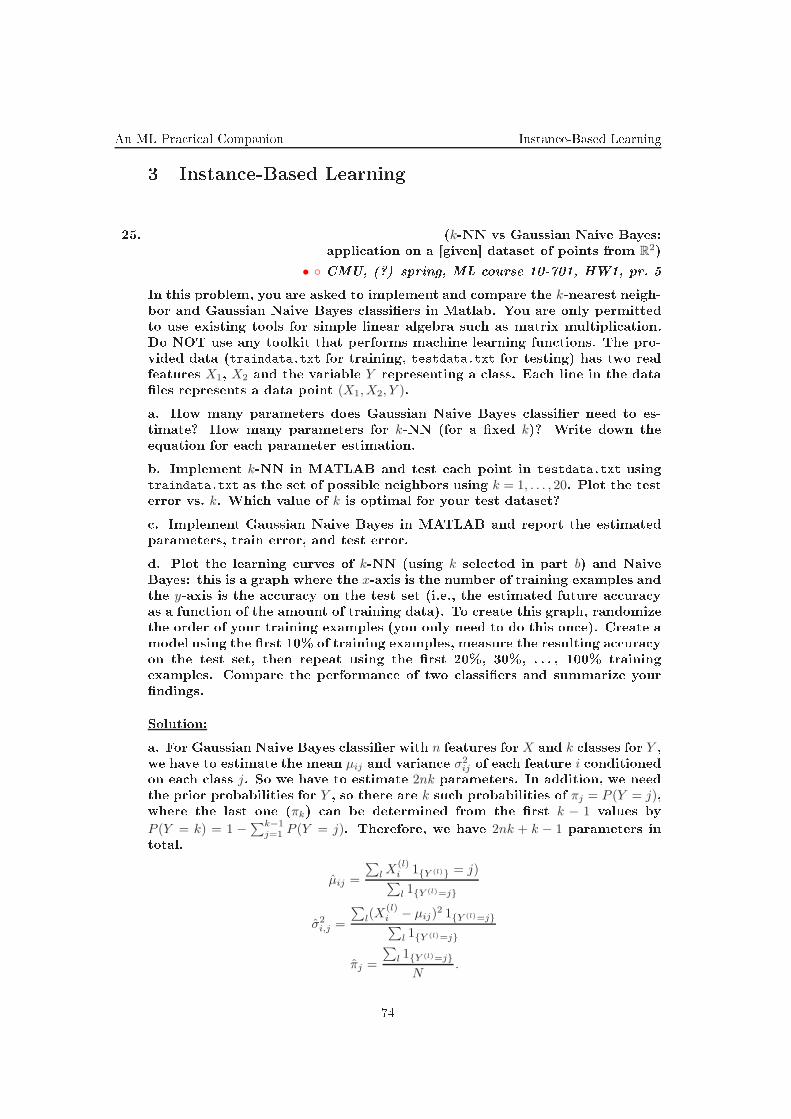
An ML Pra ti al Companion Instan e-Based Learning
3 Instan e-Based Learning
25. (k-NN vs Gaussian Naive Bayes:
xxx appli ation on a [given dataset of points from R2)
• CMU, (?) spring, ML ourse 10-701, HW1, pr. 5
In this problem, you are asked to implement and ompare the k-nearest neigh-bor and Gaussian Naive Bayes lassiers in Matlab. You are only permitted
to use existing tools for simple linear algebra su h as matrix multipli ation.
Do NOT use any toolkit that performs ma hine learning fun tions. The pro-
vided data (traindata.txt for training, testdata.txt for testing) has two real
features X1, X2 and the variable Y representing a lass. Ea h line in the data
les represents a data point (X1, X2, Y ).
a. How many parameters does Gaussian Naive Bayes lassier need to es-
timate? How many parameters for k-NN (for a xed k)? Write down the
equation for ea h parameter estimation.
b. Implement k-NN in MATLAB and test ea h point in testdata.txt using
traindata.txt as the set of possible neighbors using k = 1, . . . , 20. Plot the testerror vs. k. Whi h value of k is optimal for your test dataset?
. Implement Gaussian Naive Bayes in MATLAB and report the estimated
parameters, train error, and test error.
d. Plot the learning urves of k-NN (using k sele ted in part b) and Naive
Bayes: this is a graph where the x-axis is the number of training examples and
the y-axis is the a ura y on the test set (i.e., the estimated future a ura y
as a fun tion of the amount of training data). To reate this graph, randomize
the order of your training examples (you only need to do this on e). Create a
model using the rst 10% of training examples, measure the resulting a ura y
on the test set, then repeat using the rst 20%, 30%, . . . , 100% training
examples. Compare the performan e of two lassiers and summarize your
ndings.
Solution:
a. For Gaussian Naive Bayes lassier with n features for X and k lasses for Y ,we have to estimate the mean µij and varian e σ2
ij of ea h feature i onditionedon ea h lass j. So we have to estimate 2nk parameters. In addition, we need
the prior probabilities for Y , so there are k su h probabilities of πj = P (Y = j),where the last one (πk) an be determined from the rst k − 1 values by
P (Y = k) = 1 −∑k−1j=1 P (Y = j). Therefore, we have 2nk + k − 1 parameters in
total.
µij =
∑
l X(l)i 1Y (l) = j)∑
l 1Y (l)=j
σ2i,j =
∑
l(X(l)i − µij)
2 1Y (l)=j∑
l 1Y (l)=j
πj =
∑
l 1Y (l)=j
N.
74

Instan e-Based Learning An ML Pra ti al Companion
In the given example where we onsider two features with binary labels, we
have 8+1=9 parameters. k-NN is nonparametri method, and there is no
parameter to estimate.
b.
5 10 15 20
0.09
0.10
0.11
0.12
k
test
err
or
LC: The least test error was obtained for k = 14. However, for a better
ompromise between a ura y and e ien y (knowing that more omputa-
tions are required for omputing distan es in a spa e with a higher number
of dimensions / attributes), one might instead hoose another value for k, forinstan e k = 9.
.
µ2ij =
−0.7438 0.9717−0.9848 0.9769
σ2ij =
1.0468 0.88610.8889 1.1822
πj = 0.5100 0.4900
The training error was 0.0700, and the test error was 0.0975.
75

An ML Pra ti al Companion Instan e-Based Learning
d.
[LC: For generating the results for k-NN here it was employed the value of k hosen at part b.]
LC's observations:
1. One an see in the above graph that when 40-180 training examples are
used, the test error produ ed by the two lasssiers are very lose (slightly
lower for Gaussian Naive Bayes). For 200 training examples k-NN be omes
slightly better.
2. The varian es are in general larger for k-NN, even very large when few
training examples (less than 40) are used.
76

Instan e-Based Learning An ML Pra ti al Companion
26. (k-NN applied on hand-written digits
xxx from postal zip odes;
xxx ompare dierent methods to hoose k)
• CMU, 2004 fall, Carlos Guestrin, HW4, pr. 3.2-8
You will implement a lassier in Matlab and test it on a real data set. The
data was generated from handwritten digits, automati ally s anned from en-
velopes by the U.S. Postal Servi e. Please download the knn.data le from the
ourse web page. It ontains 364 points. In ea h row, the rst attribute is the
lass label (0 or 1), the remaining 256 attributes are features (all olumns are
ontinuous values). You ould use Matlab fun tion load('knn.data) to load
this data into Matlab.
a. Now you will implement a k-nearest-neighbor (k-NN) lassier using Ma-
tlab. For ea h unknown example, the k-NN lassier olle ts its k nearest
neighbors training points, and then takes the most ommon ategory among
these k neighbors as the predi ted label of the test point.
We assume our lassi ation is a binary lassi ation task. The lass label
would be either 0 or 1. The lassier uses the Eu lidean distan e metri .
(But you should keep in mind that normal k-NN lassier supports multi-
lass lassi ation.) Here is the prototype of the Matlab fun tion you need to
implement:
fun tion[Y_test = knn(k, X_train, Y_train, X_test);
X_train ontains the features of the training points, where ea h row is a 256-
dimensional ve tor. Y_train ontains the known labels of the training points,
where ea h row is an 1-dimensional integer either 0 or 1. X_test ontains the
features of the testing points, where ea h row is a 256-dimensional ve tor.
k is the number of nearest-neighbors we would onsider in the lassi ation
pro ess.
b. For k = 2, 4, 6, . . ., you may en ounter ties in the lassi ation. Des ribe
how you handle this situation in your above implementation.
. The hoi e of k is essential in building the k-NN model. In fa t, k an be
regarded as one of the most important fa tors of the model that an strongly
inuen e the quality of predi tions.
One simple way to nd k is to use the train-test style. Randomly hoose 30%
of your data to be a test set. The remainder is a training set. Build the
lassi ation model on the training set and estimate the future performan e
with the test set. Try dierent values of k to nd whi h works best for the
testing set.
Here we use the error rate to measure the performan e of a lassier. It
equals to the per entage of in orre tly lassied ases on a test set.
Please implement a Matlab fun tion to implement the above train-test way
for nding a good k for the kNN lassier. Here is the prototype of the Matlab
fun tion you need to implement:
fun tion[TestsetErrorRate, TrainsetErrorRate =
knn_train_test(kArrayToTry, XData, YData);
77

An ML Pra ti al Companion Instan e-Based Learning
XData ontains the features of the data points, where ea h row is a 256-
dimensional ve tor. YData ontains the known labels of the points, where ea h
row is an 1-dimensional integer either 0 or 1. kArrayToTry is a k × 1 olumn
ve tor, ontaining the k possible values of k you want to try. TestsetErrorRate
is a k × 1 olumn ve tor ontaining the testing error rate for ea h possible k.TrainsetErrorRate is a k × 1 olumn ve tor ontaining the training error rate
for ea h possible k.
Then test your fun tion knn_train_test on data set knn.data.
Report the plot of train error rate vs. k and the plot of test error rate vs. kfor this data. (Make these two urves together in one gure. You ould use
hold on fun tion in Matlab to help you.) What is the best k you would hoose
a ording to these two plots?
d. Instead of the above train-test style, we ould also do n-folds Cross-
validation to nd the best k. n-folds Cross-validation is a well established
te hnique that an be used to obtain estimates of model parameters that are
unknown. The general idea of this method is to divide the data sample into
a number of n folds (randomly drawn, disjointed sub-samples or segments).
For a xed value of k, we apply the k-NN model to make predi tions on the
i-th segment (i.e., use the n− 1 segments as the train examples) and evaluate
the error. This pro ess is then su essively applied to all possible hoi es of
i (i ∈ 1, . . . , v). At the end of the n folds ( y les), the omputed errors are
averaged to yield a measure of the stability of the model (how well the model
predi ts query points). The above steps are then repeated for various k and
the value a hieving the lowest error rate is then sele ted as the optimal value
for k (optimal in a ross-validation sense).
721
Then please implement a ross-validation fun tion to hoose k. Here is the
prototype of the Matlab fun tion you need to implement:
fun tion[ vErrorRate = knn_ v(kArrayToTry, XData, YData, numCVFolds);
All the dimensionality of input parameters are the same as in part c. vErrorRateis a k× 1 olumn ve tor ontaining the ross validation error rate for ea h po-
ssible k.
Apply this fun tion on the data set knn.data using 10- ross-folds. Report a
performan e urve of ross validation error rate vs. k. What is the best k youwould hoose a ording to this urve?
e. Besides the train-test style and n-folds ross validation, we ould also
use leave-one-out Cross-validation (LOOCV) to nd the best k. LOOCV
means omitting ea h training ase in turn and train the lassier model on
the remaining R − 1 datapoints, test on this omitted training ase. When
you've done all points, report the mean error rate. Implement a LOOCV
fun tion to hoose k for our k-NN lassier. Here is the prototype of the
matlab fun tion you need to implement:
fun tion[Loo vErrorRate = knn_loo v(kArrayToTry, XData, YData);
721
If you want to understand more about ross validation, please look at Andrew Moore's Cross-Validation
slides online: http://www-2. s. mu.edu/ awm/tutorials/overt.html.
78

Instan e-Based Learning An ML Pra ti al Companion
All the dimensionality of input parameters are the same as in part c.Loo vErrorRate is a k× 1 olumn ve tor ontaining LOOCV error rate for ea h
possible k.
Apply this fun tion on the data set knn.data and report the performan e urve
of LOOCV error rate vs. k. What is the best k you would hoose a ording
to this urve?
f. Compare the four performan e urves (from parts c, d and e). Make the
four urves together in one gure here. Can you get some on lusion about
the dieren e between train-test, n-folds ross-validation and leave-one-out
ross validation?
Note: We provide a Matlab le TestKnnMain.m to help you test the above
fun tions. You ould download it from the ourse web site.
Solution:
b. There are many possible ways to handle this tie ase. For example, i.
hoose one of the lass; ii. use k − 1 neighbor to de ide; iii. weighted k-NN,et .
-f. We would get four urves roughly having the similar trend. The best
error rate is around 0.02. If you run the program several times, you would
nd that LOOCV urve would be the same among multiple runs, be ause it
does not have randomness involved. CV urves varies roughly around the
LOOCV urve. The train-test test urve varies a lot among dierent runs.
But anyway, roughly, as k in reases, the error rate in reases. From the urve,
we an a tually hoose a small range of k (1− 5) as our model sele tion result.
79

An ML Pra ti al Companion Instan e-Based Learning
27. (k-NN and SVM: appli ation on
xxx a fa ial attra tiveness task)
• CMU, 2007 fall, Carlos Guestrin, HW3, pr. 3
xxx CMU, 2009 fall, Carlos Guestrin, HW3, pr. 3
In this question, you will explore how ross-validation an be used to t ma-
gi parameters. More spe i ally, you'll t the onstant k in the k-NearestNeighbor algorithm, and the sla k penalty C in the ase of Support Ve tor
Ma hines.
Dataset
Download the le hw3_matlab.zip and unpa k it. The le fa es.mat ontains
the Matlab variables traindata (training data), trainlabels (training labels),
testdata (test data), testlabels (test labels) and evaldata (evaluation data,
needed later).
This is a fa ial attra tiveness lassi ation task: given a pi ture of a fa e, you
need to predi t whether the average rating of the fa e is hot or not. So, ea h
row orresponds to a data point (a pi ture). Ea h olumn is a feature, a pixel.
The value of the feature is the value of the pixel in a grays ale image.
722
For
fun, try showfa e(evaldata(1,:)), showfa e(evaldata(2,:)), . . . .
osineDistan e.m implements the osine distan e, a simple distan e fun tion.
It takes two feature ve tors x and y, and omputes a nonnegative, symmetri
distan e between x and y. To he k your data, ompute the distan e between
the rst training example from ea h lass. (It should be 0.2617.)
A. k-NN
a. Implement the k-Nearest Neighbor (k-NN) algorithm in Matlab. Hint:
You might want to pre ompute the distan es between all pairs of points, to
speed up the ross-validation later.
b. Implement n-fold ross validation for k-NN. Your implementation should
partition the training data and labels into n parts of approximately equal size.
. For k = 1, 2, . . . , 100, ompute and plot the 10-fold (i.e., n = 10) ross-
validation error for the training data, the training error, and the test error.
How do you interpret these plots? Does the value of k whi h minimizes the
ross-validation error also minimize the test set error? Does it minimize the
training set error? Either way, an you explain why? Also, what does this
tell us about using the training error to pi k the value of k?
B. SVM
d. Now download libsvm using the link from the ourse website and unpa k it
to your working dire tory. It has a Matlab interfa e whi h in ludes binaries
for Windows. It an be used on OS X or Unix but has to be ompiled (requires
g++ and make) see the README le from the libsvm zip pa kage.
hw3_matlab.zip, whi h you downloaded earlier, ontains les testSVM.m (an
example demonstration s ript), trainSVM.m (for training) and lassifySVM.m
722
This is an easier version of the dataset presented in Ryan White, Ashley Eden, Mi hael Maire Automati
Predi tion of Human Attra tiveness, CS 280 lass report, De ember 2003 on the proje t website.
80

Instan e-Based Learning An ML Pra ti al Companion
(for lassi ation), whi h will show you how to use libsvm for training and
lassifying using an SVM. Run testSVM. This should report a test error of
0.4333.
In order to train an SVM with sla k penalty C on training set data with labels
labels, all
svmModel = trainSVM(data, labels, C)
In order to lassify examples test, all
testLabels = lassifySVM(svmModel, test)
Train an SVM on the training data with C = 500, and report the error on the
test set.
e. Now implement n-fold ross-validation for SVMs.
f. For C = 10, 102, 103, 104, 5 · 104, 105, 5 · 105, 106, ompute and plot the 10-fold
(i.e., n = 10) ross-validation error for the training data, the training error,
and the test error, with the axis for C in log-s ale (try semilogx).
How do you interpret these plots? Does the value of C whi h minimizes the
ross-validation error also minimize the test set error? Does it minimize the
training set error? Either way, an you explain why? Also, what does this
tell us about using the training error to pi k the value of C?
81
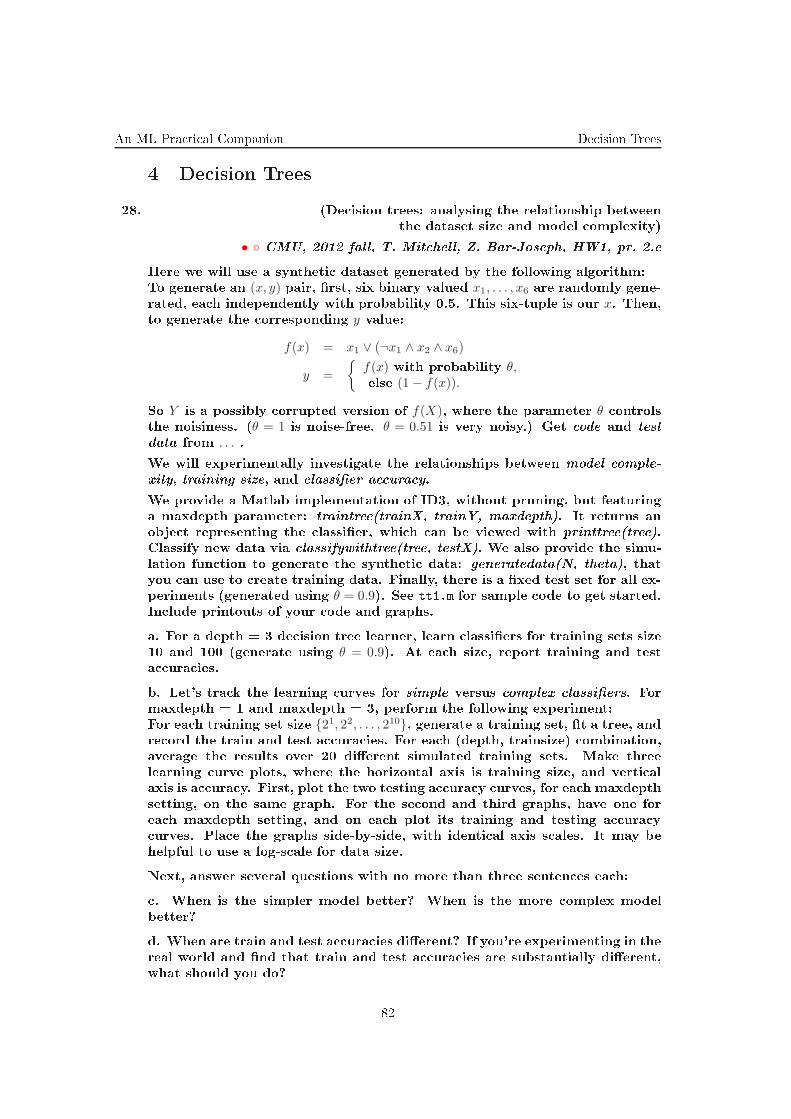
An ML Pra ti al Companion De ision Trees
4 De ision Trees
28. (De ision trees: analysing the relationship between
xxx the dataset size and model omplexity)
• CMU, 2012 fall, T. Mit hell, Z. Bar-Joseph, HW1, pr. 2.e
Here we will use a syntheti dataset generated by the following algorithm:
To generate an (x, y) pair, rst, six binary valued x1, . . . , x6 are randomly gene-
rated, ea h independently with probability 0.5. This six-tuple is our x. Then,to generate the orresponding y value:
f(x) = x1 ∨ (¬x1 ∧ x2 ∧ x6)
y =
f(x) with probability θ,else (1− f(x)).
So Y is a possibly orrupted version of f(X), where the parameter θ ontrolsthe noisiness. (θ = 1 is noise-free. θ = 0.51 is very noisy.) Get ode and test
data from . . . .
We will experimentally investigate the relationships between model omple-
xity, training size, and lassier a ura y.
We provide a Matlab implementation of ID3, without pruning, but featuring
a maxdepth parameter: traintree(trainX, trainY, maxdepth). It returns an
obje t representing the lassier, whi h an be viewed with printtree(tree).
Classify new data via lassifywithtree(tree, testX). We also provide the simu-
lation fun tion to generate the syntheti data: generatedata(N, theta), that
you an use to reate training data. Finally, there is a xed test set for all ex-
periments (generated using θ = 0.9). See tt1.m for sample ode to get started.
In lude printouts of your ode and graphs.
a. For a depth = 3 de ision tree learner, learn lassiers for training sets size
10 and 100 (generate using θ = 0.9). At ea h size, report training and test
a ura ies.
b. Let's tra k the learning urves for simple versus omplex lassiers. For
maxdepth = 1 and maxdepth = 3, perform the following experiment:
For ea h training set size 21, 22, . . . , 210, generate a training set, t a tree, andre ord the train and test a ura ies. For ea h (depth, trainsize) ombination,
average the results over 20 dierent simulated training sets. Make three
learning urve plots, where the horizontal axis is training size, and verti al
axis is a ura y. First, plot the two testing a ura y urves, for ea h maxdepth
setting, on the same graph. For the se ond and third graphs, have one for
ea h maxdepth setting, and on ea h plot its training and testing a ura y
urves. Pla e the graphs side-by-side, with identi al axis s ales. It may be
helpful to use a log-s ale for data size.
Next, answer several questions with no more than three senten es ea h:
. When is the simpler model better? When is the more omplex model
better?
d. When are train and test a ura ies dierent? If you're experimenting in the
real world and nd that train and test a ura ies are substantially dierent,
what should you do?
82

De ision Trees An ML Pra ti al Companion
e. For a parti ular maxdepth, why do train and test a ura ies onverge to the
same pla e? Comparing dierent maxdepths, why do test a ura ies onverge
to dierent pla es? Why does it take smaller or larger amounts of data to do
so?
f. For maxdepths 1 and 3, repeat the same vary-the-training-size experiment
with θ = 0.6 for the training data. Show the graphs. Compare to the previous
ones: what is the ee t of noisier data?
Solution:
a.
b. Pink stars: depth = 3. Bla k x's: depth = 1. Blue ir les: training
a ura y. Red squares: testing a ura y.
. It is good to have high model omplexity when there is lots of training
data. When there is little training data, the simpler model is better.
d. They're dierent when you're overtting. If this is happening you have
two options: (1) de rease your model omplexity, or (2) get more data.
e. They onverge when the algorithm is learning the best possible model
from the model lass pres ribed by maxdepth: this gets same a ura y on the
training and test sets. (2) The higher omplexity (maxdepth=3) model lass
learns the underlying fun tion better, thus gets better a ura y. But, (3) the
higher omplexity model lass has more parameters to learn, and thus takes
more data to get to this point.
f. It's mu h harder for the omplex model to do better. Also, it takes mu h
longer for all test urves to onverge. (Train/test urves don't onverge to
same pla e be ause noise levels are dierent.)
Note: Colors and styles are the same as for previous plots. These plots test
all the way up to 215 training examples: you an see where they onverge to,
whi h is not ompletely lear with only 210 examples.
83

An ML Pra ti al Companion De ision Trees
29. (De ision trees: experiment
xxx with an ID3 implementation (in C))
• CMU, 2012 spring, Roni Rosenfeld, HW3
This exer ise gives you the opportunity to experiment with a de ision tree
learning program. You are rst asked to experiment with the simple Play-
Tennis data des ribed in Chapter 3 of TomMit hell'sMa hine Learning book,
and then to experiment with a onsiderably larger data set.
We provide most of the de ision tree ode. You will have to omplete the
ode, test, and prune a de ision tree based on the ID3 algorithm des ribed in
Chapter 3 of the textbook. You an obtain it as a gzipped ar hive from . . . .
To unzip and get started on a Linux/Ma ma hine, do the following:
1. Download the hw3.tgz le to your working dire tory.
2. Issue the ommand tar -zxvf hw3.tgz to unzip and untar the le. This will
reate a subdire tory hw3 in the urrent dire tory.
3. Type make to ompile and you are ready to go. The exe utable is alled
dt. There is a help le named README.dt whi h ontains instru tions on how
to run the dt program.
If you work from a Windows ma hine, you an install Cygwin and that should
give you a Linux environment. Remember to install the Devel ategory to
get g . Depending on your ma hine some tweaks might be needed to make
it work.
A. Play Tennis Data
The training data from Table 3.2 in the textbook is available in the le
tennis.ssv. Noti e that it ontains the fourteen training examples repeated
twi e. For question A.2, please use it as given (with the 28 training exam-
ples). For question A.4, you will need to extra t the fourteen unique training
examples and use those in addition to the ones you invent.
A1. If you try running the ode now it will not work be ause the fun tion that
al ulates the entropy has not been implemented. (Remember that entropy is
required in turn to ompute the information gain.) It is your job to omplete
it. You will have to make your hanges in the le entropy. . After you
orre tly implement the entropy al ulation, the program will produ e the
de ision tree shown in Figure 3.1 of the textbook when run on tennis.ssv
(with all examples used for training).
Hint: When you implement the entropy fun tion, be sure to deal with asts
from int to double orre tly. Note that num_pos/num_total = 0 if num_pos and
num_total are both int's. You must do ((double)num_pos)/num_total to get the
desired result or, alternately, dene num_total as a double.
A2. Try running the program a few times with half of the data set for training
and the other half for testing (no pruning). Print out your ommand for
running the program. Do you get a dierent result ea h time? Why? Report
the average a ura y of 10 runs on both training and test data (use the bat h
option of dt). For this question please use tennis.ssv as given.
A3. If we add the following examples:
84

De ision Trees An ML Pra ti al Companion
0 sunny hot high weak
1 sunny ool normal weak
0 sunny mild high weak
0 rain mild high strong
1 sunny mild normal strong
to the original tennis.ssv that has 28 examples, whi h attribute would be
sele ted at the root node? Compute the information gain for ea h attribute
and nd out the max. Show how you al ulate the gains.
A4. By now, you should be able to tea h ID3 the on ept represented by
Figure 3.1; we all this the orre t on ept. If an example is orre tly labeled
by the orre t on ept, we all the example a orre t example. For this ques-
tion, you will need to extra t the fourteen unique examples from tennis.ssv.
In ea h of the questions below, you will add some your own examples to the
original fourteen, and use all of them for training (You will not use a testing
or pruning set here.). Turn in your datasets (named a ording to the Hand-in
se tion at the end).
a. Dupli ate some of the fourteen training examples in order to get ID3 to
learn a dierent de ision tree.
b. Add new orre t samples to the original fourteen samples in order to get
ID3 to in lude the attribute temperature in the tree.
A5. Use the fourteen unique examples from tennis.ssv. Run ID3 on e using
all fourteen for training, and note the stru ture (whi h is in Figure 3.1). Now,
try ipping the label (0 to 1, or 1 to 0) of any one example, and run ID3 again.
Note the stru ture of the new tree.
Now hange the example's label ba k to orre t. Do the same with another
four samples. (Flip one label, run ID3, and then ip the label ba k.) Give
some general observations about the stru tures (dieren es and similarities
with the original tree) ID3 learns on these slightly noisy datasets.
B. Agari us-Lepiota Data Set
The le mushroom.ssv ontains re ords drawn from The Audobon So iety Fi-
eld Guide to North Ameri an Mushrooms (1981), G. H. Lin o (Pres.), New
York. Alfred A. Knopf, posted [LC: it on the UCI Ma hine Learning Repo-
sitory. Ea h re ord ontains information about a mushroom and whether or
not it is poisonous.
B1. First we will look at how the quality of the learned hypothesis varies
with the size of the training set. Run the program with training sets of size
10%, 30%, 50%, 70%, and 90%, using 10% to test ea h time. Please run a
parti ular size at least 10 times. You may want to use the bat h mode option
provided by dt.
Constru t a graph with training set size on the x-axis and test set a ura y
on the y-axis. Remember to pla e errorbars on ea h point extending one
standard deviation above and below the point. You an do this in Matlab,
Mathemati a, GNUplot or by hand.
If you use gnuplot:
1. Create a le data.txt with your results with the following format:
2. Ea h line has <training size> <a ura y> <standard deviation>.
85

An ML Pra ti al Companion De ision Trees
3. Type gnuplot to get to the gnuplot ommand prompt. At the prompt,
type set terminal posts ript followed by set output graph.ps and nally plot
data.txt with errorbars to plot the graph.
B2. Now repeat the experiment, but with a noisy dataset, noisy10.ssv, in
whi h ea h label in has been ipped with a han e of 10%. Run the program
with training sizes from 30% to 70% at the step of 5% (9 sizes in total), using
10% at ea h step to test and at least 10 trials for ea h size. Plot the graph
of test a ura y and ompare it with the one from B.1. In addition, plot
the number of nodes in the result trees against the training %. Note that
the training a ura y de reases slightly after a ertain point. You may also
observe dips in the test a ura y. What ould be ausing this?
B3. One way to battle these phenomena is with pruning. For this question,
you will need to omplete the implementation of pruning that has been pro-
vided. As it stands, the pruning fun tion onsiders only the root of the tree
and does not re ursively des end to the sub-trees. You will have to x this by
implementing the re ursive all in PruneDe isionTree() (in prune-dt. ). Re all
that pruning traverses the tree removing nodes whi h do not help lassi a-
tion over the validation set. Note that pruning a node entails removing the
sub-tree(s) below a node, and not the node itself.
In order to implement the re ursive all, you will need to familiarize yourself
with the trees representation in C. In parti ular, how to get at the hildren of
a node. Look at dt.h for details. A de ision you will make is when to prune
a sub-tree, before or after pruning the urrent node. Bottom-Up pruning
is when you prune the subtree of a node, before onsidering the node as a
pruning andidate. Top-down pruning is when you rst onsider the node
as a pruning andidate and only prune the subtree should you de ide not to
eliminate the node. Please do NOT mix the two up. If you are in doubt,
onsult the book.
Write out on paper the ode that you would need to add for both bottom-up
and top-down pruning. Implement only the bottom-up ode and repeat the
experiments in B.2 using 20% of the data for pruning at ea h trial. Plot the
graph of test a ura y and number of nodes and omment on the dieren es
from B.2.
B4. Answer the following questions with explanation.
a. Whi h pruning strategy would make more alls? top-down or bottom-up?
or is it data-dependent?
b. Whi h pruning strategy would result in better a ura y on the pruning
set? top-down or bottom-up? or is it data-dependent?
. Whi h pruning strategy would result in better a ura y on the testing set?
top-down or bottom-up? or is it data-dependent?
Hand-In Instru tions
Besides your assignment write-up, here is the additional materials you will
need to hand in. Your write-up should in lude the graphs asked for.
A.1. Hand in your modied entropy. .
A.2. Nothing to hand in.
A.3. Nothing to hand in.
86

De ision Trees An ML Pra ti al Companion
A.4. For part a, hand in tennis1.4.a.ssv, whi h should ontain the original
data plus the samples you reated appended at the end of the le. Likewise
for b.
B.1. Nothing to hand in.
B.2. Nothing to hand in.
B.3. Hand in your modied prune-dt. .
B.4. Nothing to hand in.
Hints:
− If you are unsure about your answer, play with ode to see if you an
experimentally verify your intuitions.
− It is very helpful to in lude explanations with your examples, or at least
mention how you onstru ted the example, what was the reasoning behind
your hoi es, et .
− Please label the axes and spe ify what a ura y/performan e metri you
are measuring and on what dataset: e.g. training, testing, validation, noisy10
et .
Solution:
A1. The Entropy fun tion should be like:
double Entropy( int num_pos, int num_neg )
if (num_pos == 0 || num_neg == 0)
return 0.0;
double entropy = 0.0;
double total = (double) (num_pos + num_neg);
entropy = - (num_pos / total) * LogBase2( num_pos / total )
- (num_neg / total) * LogBase2( num_neg / total );
return entropy;
A2. The ommand is: ./dt 0.5 0 0.5 tennis.ssv
The results are dierent, be ause the ode randomly splits the data, and ea h
time a dierent training set is used.
The training a ura y is always 100%. The testing a ura y should be around
82%.
A3. The data set now has 13 negatives and 20 positives. So the overall entropy
is: 0.967.
Using outlook, the information gain is: 0.218.
Using temperature, the information gain is: 0.047.
Using humidity, the information gain is: 0.221.
Using wind, the information gain is: 0.025.
Therefore, humidity should be sele ted.
A4.
87

An ML Pra ti al Companion De ision Trees
a. Examples given in question A.3 are a tually dupli ates that hanged the
tree.
b. The idea is to let temperature determine Play-Tennis. For example, we
an add the following:
1 sunny ool normal weak
1 over ast ool normal weak
1 rain ool normal weak
1 sunny ool normal weak
0 rain hot normal strong
0 sunny hot high weak
0 sunny hot high weak
0 rain hot normal strong
A5. Generally, noisy data sets produ e bigger trees. However the rules im-
plied by these trees are quite stable. Some trees may have the same top
stru ture as the true stru ture. These overall similarities to the true stru -
ture give some intuition for why pruning helps; pruning an ut away the
extra subtrees whi h model small ee ts whi h might be from noise.
B1. I ran ea h size 20 times, and got a graph like this:
B2.
88

De ision Trees An ML Pra ti al Companion
This de rease in testing a ura y with the larger training may be aused by
a form of overtting; that is, the algorithm tries to perfe tly mat h the data
in the training set, in luding the noise, and as a result the omplexity of
the learned tree in reases very rapidly as the number of training examples
in reases.
Note that this is not the usual sense of overtting, sin e typi ally overtting is
more of a problem when the number of training examples is small. However,
here we also have the problem that the omplexity of the hypothesis spa e
is an in reasing fun tion of the number of training examples. See how the
number of nodes grows.
There are also dips in the a ura y on the test set, a point where the a -
ura y de reased before in reasing again. This is be ause of more omplex
on epts; there are always two ompeting for es here: the information ontent
of the training data, whi h in reases with the number of training examples
and pushes toward higher a ura ies, and the omplexity of the hypothesis
spa e, whi h gets worse as the number of training examples in reases.
You may also noti e that the training a ura y slightly de reases as the size
of the training set grows. This seems to be purely due to the noisy labels,
whi h makes it impossible to onstru t a onsistent tree, and the more pairs
of examples you have in the training set that have ontradi ting labels, the
worse will be the training error.
B3.
For bottom-up pruning, add to the beginning of the fun tion:
/*******************************************************************
You ould insert the re ursive all BEFORE you he k the node
*******************************************************************/
for (i = 0 ; i < node->num_ hildren ; i++)
PruneDe isionTree(root, node-> hildren[i, data, num_data, pruning_set, num_prune, ssvinfo);
For top-down pruning, add to the end of the fun tion:
/*******************************************************************
Or you ould do the re ursive all AFTER you he k the node
(given that you de ided to keep it)
*******************************************************************/
for (i = 0 ; i < node->num_ hildren ; i++)
PruneDe isionTree(root, node-> hildren[i, data, num_data, pruning_set, num_prune, ssvinfo);
89

An ML Pra ti al Companion De ision Trees
By running ea h size 20 times I got a graph like this:
B4.
a. Bottom-up. Bottom-up pruning examines all the nodes. Top-down pruning
may eliminate a subtree without examining the nodes in the subtree, leading
to fewer alls than bottom-up.
b. Bottom-up. By the property of the algorithm, bottom-up pruning returns
the tree with the LOWEST POSSIBLE ERROR over the pruning set. Sin e
top-down an aggressively eliminate subtree's without onsidering ea h of the
nodes in the subtree, it ould return a non-optimal tree (over the pruning
set that is). Keep in mind that the fun tion used to de ide whether a node
should be removed or not is the same for both BU and TD and only the sear h
strategy diers.
. Data depedent. If the test set is very dierent from the training set, a
shorter tree yielded by top-down pruning may perform better, be ause of its
potentially better generalization power.
90

De ision Trees An ML Pra ti al Companion
30. (ID3 with ontinuous attributes:
xxx experiment with a Matlab implementation
xxx on the Breast Can er dataset)
• CMU, 2011 fall, T. Mit hell, A. Singh, HW1, pr. 2
One very interesting appli ation area of ma hine learning is in making medi al
diagnoses. In this problem you will train and test a binary de ision tree to
dete t breast an er using real world data. You may use any programming
language you like.
The Dataset
We will use the Wis onsin Diagnosti Breast Can er (WDBC) dataset
723
The
dataset onsists of 569 samples of biopsied tissue. The tissue for ea h sample
is imaged and 10 hara teristi s of the nu lei of ells present in ea h image
are hara terized. These hara teristi s are
(a) Radius
(b) Texture
( ) Perimeter
(d) Area
(e) Smoothness
(f) Compa tness
(g) Con avity
(h) Number of on ave portions of ontour
(i) Symmetry
(j) Fra tal dimension
Ea h of the 569 samples used in the dataset onsists of a feature ve tor of
length 30. The rst 10 entries in this feature ve tor are the mean of the
hara teristi s listed above for ea h image. The se ond 10 are the standard
deviation and last 10 are the largest value of ea h of these hara teristi s
present in ea h image.
Ea h sample is also asso iated with a label. A label of value 1 indi ates the
sample was for malignant ( an erous) tissue. A label of value 0 indi ates the
sample was for benign tissue.
This dataset has already been broken up into training, validation and test sets
for you and is available in the ompressed ar hive for this problem on the lass
website. The names of the les are trainX. sv, trainY. sv, validationX. sv,
validationY. sv, testX. sv and testY. sv. The le names ending in X. sv
ontain feature ve tors and those ending in Y. sv ontain labels. Ea h le is
in omma separated value format where ea h row represents a sample.
A. Programming
A1. Learning a binary de ision tree
As dis ussed in lass and the reading material, to learn a binary de ision tree
we must determine whi h feature attribute to sele t as well as the threshold
723
Original dataset available at http://ar hive.i s.u i.edu/ml/datasets/Breast+Can er+Wis onsin+(Diagnosti ).
91
An ML Pra ti al Companion De ision Trees
value to use in the split riterion for ea h non-leaf node in the tree. This
an be done in a re ursive manner, where we rst nd the optimal split for
the root node using all of the training data available to us. We then split
the training data a ording to the riterion sele ted for the root node, whi h
will leave us with two subsets of the original training data. We then nd
the optimal split for ea h of these subsets of data, whi h gives the riterion
for splitting on the se ond level hildren nodes. We re ursively ontinue this
pro ess until the subsets of training data we are left with at a set of hildren
nodes are pure (i.e., they ontain only training examples of one lass) or the
feature ve tors asso iated with a node are all identi al (in whi h ase we an
not split them) but their labels are dierent.
In this problem, you will implement an algorithm to learn the stru ture of a
tree. The optimal splits at ea h node should be found using the information
gain riterion dis ussed in lass.
While you are free to write your algorithm in any language you hoose, if
you use the provided Matlab ode in luded in the ompressed ar hive for
this problem on the lass website, you only need to omplete one fun tion,
omputeOptimalSplit.m. This fun tion is urrently empty and only ontains
omments des ribing how it should work. Please omplete this fun tion so
that given any set of training data it nds the optimal split a ording to the
information gain riterion.
In lude a printout of your ompleted omputeOptimalSplit.m along with any
other fun tions you needed to write with your homework submission. If you
hoose to not use the provided Matlab ode, please in lude a printout of all
the ode you wrote to train a binary de ision tree a ording to the des ription
given above.
Note: While there are multiple ways to design a de ision tree, in this problem
we onstrain ourselves to those whi h simply pi k one feature attribute to split
on. Further, we restri t ourselves to performing only binary splits. In other
words, ea h split should simply determine if the value of a parti ular attribute
in the feature ve tor of a sample is less than or equal to a threshold value or
greater than the threshold value.
Note: Please note that the feature attributes in the provided dataset are
ontinuously valued. There are two things to keep in mind with this.
First, this is slightly dierent than working with feature values whi h are
dis rete be ause it is no longer possible to try splitting at every possible
feature value (sin e there are an innite number of possible feature values).
One way of dealing with this is by re ognizing that given a set of training data
of N points, there are only N − 1 pla es we ould pla e splits for the data (if
we onstrain ourselves to binary splits). Thus, the approa h you should take
in this fun tion is to sort the training data by feature value and then test split
values that are the mean of ordered training points. For example, if the points
to split between were 1, 2, 3, you would test two split values: 1.5 and 2.5.
Se ond, when working working with feature values that an only take on one
of two values, on e we split using one feature attribute, there is no point in
trying to split on that feature attribute later. (Can you think of why this
would be?) However, when working with ontinuously valued data, this is no
longer the ase, so your splitting algorithm should onsider splitting on all
feature attributes at every split.
92

De ision Trees An ML Pra ti al Companion
A2. Pruning a binary de ision tree
The method of learning the stru ture and splitting riterion for a binary de-
ision tree des ribed above terminates when the training examples asso iated
with a node are all of the same lass or there are no more possible splits.
In general, this will lead to overtting. As dis ussed in lass, pruning is one
method of using validation data to avoid overtting.
You will implement an algorithm to use validation data to greedily prune
a binary de ision tree in an iterative manner. Spe i ally, the algorithm
that we will implement will start with a binary de ision tree and perform an
exhaustive sear h for the single node for whi h removing it (and its hildren)
produ es the largest in rease (or smallest de rease) in lassi ation a ura y
as measured using validation data. On e this node is identied, it and its
hildren are removed from the tree, produ ing a new tree. This pro ess is
repeated, where we iteratively prune one node at a time until we are left with
a tree whi h onsists only of the root node.
724
Implement a fun tion whi h starts with a tree and sele ts the single best
node to remove in order to produ e the greatest in rease (or smallest de-
rease) in lassi ation a ura y as measured with validation data. If you
are using Matlab, this means you only need to omplete the empty fun tion
pruneSingleGreedyNode.m. Please see the omments in that fun tion for de-
tails on what you should implement. We suggest that you make use of the
provided Matlab fun tiona pruneAllNodes.m whi h will return a listing of all
possible trees that an be formed by removing a single node from a base tree
and bat hClassifyWithDT.m whi h will lassify a set of samples given a de ision
tree.
Please in lude your version of pruneSingleGreedyNode.m along with any other
fun tions you needed to write with your homework. If not using Matlab,
please atta h the ode for a fun tion whi h performs the same fun tion des-
ribed for pruneSingleGreedyNode.m.
B. Data analysis
B1. Training a binary de ision tree
In this se tion, we will make use of the ode that we have written above.
We will start by training a basi de ision tree. Please use the training data
provided to train a de ision tree. (In Matlab, assuming you have ompleted
the omputeOptimalSplit.m fun tion, the fun tion trainDT.m an do this training
for you.)
Please spe ify the total number of nodes and the total number of leaf nodes
in the tree. (In Matlab, the fun tion gatherTreeStats.m will be useful.) Also,
please report the lassi ation a ura y (per ent orre t) of the learned de i-
sion tree on the provided training and testing data. (In Matlab, the fun tion
bat hClassifyWithDT.m will be useful.)
B2. Pruning a binary de ision tree
724
In pra ti e, you an often simply ontinue the pruning pro ess until the validation error fails to in rease by
a predened amount. However, for illustration purposes, we will ontinue until there is only one node left in the
tree.
93
An ML Pra ti al Companion De ision Trees
Now we will make use of the pruning ode we have written. Please start
with the tree that was just trained in the previous part of the problem and
make use of the validation data to iteratively remove nodes in the greedy
manner des ribed in the se tion above. Please ontinue iterations until a
degenerate tree with only a single root node remains. For ea h tree that
is produ ed, please al ulate the lassi ation a ura y for that tree on the
training, validation and testing datasets.
After olle ting this data, please plot a line graph relating lassi ation a u-
ra y on the test set to the number of leaf nodes in ea h tree (so number of
leaf nodes should be on the X-axis and lassi ation a ura y should be on
the Y-Axis). Please add to this same gure, similar plots for per ent a ura y
on training and validation data. The number of leaf nodes should range from
1 (for the degenerate tree) to the the number present in the unpruned tree.
The Y-axis should be s aled between 0 and 1.
Please omment on what you noti e and how this illustrates overtting. In-
lude the produ ed gure and any ode you needed to write to produ e the
gure and al ulate intermediate results with your homework submission.
B3. Drawing a binary de ision tree
One of the benets of de ision trees is the lassi ation s heme they en ode
is easily understood by humans. Please sele t the binary de ision tree from
the pruning analysis above that produ ed the highest a ura y on the vali-
dation dataset and diagram it. (In the event that two trees have the same
a ura y on validation data, sele t the tree with the smaller number of leaf
nodes.) When stating the feature attributes that are used in splits, please
use the attribute names (instead of index) listed in the dataset se tion of this
problem. (If using the provided Matlab ode, the fun tion trainDT has a se -
tion of omments whi h des ribes how you an interpret the stru ture used
to represent a de ision tree in the ode.)
Hint: The best de ision tree as measured on validation data for this problem
should not be too ompli ated, so if drawing this tree seems like a lot of work,
then something may be wrong.
B4. An alternative splitting method
While information gain is one riterion to use when estimating the optimal
split, it is by no means the only one. Consider instead using a riterion where
we try to minimize the weighted mis lassi ation rate.
Formally, assume a set of D data samples < ~x(i), y(i) >Di=1, where y(i) is thelabel of sample i, and ~x(i)
is the feature ve tor for sample i. Let x(j)(i) referto the value of the jth attribute of the feature ve tor for data point i.
Now, to pi k a split riterion, we pi k a feature attribute, a, and a threshold
value, t, to use in the split. Let:
pbelow
(a, t) =1
D
D∑
i=1
I
(
x(a)(i) ≤ t)
pabove
(a, t) =1
D
D∑
i=1
I
(
x(a)(i) > t)
94

De ision Trees An ML Pra ti al Companion
and let:
lbelow
(a, t) = Mode
(
yii:x(a)(i)≤t
)
labove
(a, t) = Mode
(
yii:x(a)(i)>t
)
The split that minimizes the weighted mis lassi ation rate is then the one
whi h minimizes:
O(a, t) =pbelow
(a, t)∑
i:x(a)(i)≤t
I
(
y(i) 6= lbelow
(a, t))
+
pabove
(a, t)∑
i:x(a)(i)>t
I
(
y(i) 6= labove
(a, t))
Please modify the ode for your omputeOptimalSplit.m (or equivalent fun tion
if not using Matlab) to perform splits a ording to this riterion. Atta h the
ode of your modied fun tion when submitting your homework.
After modifying omputeOptimalSplit.m, please retrain a de ision tree (without
doing any pruning). In your homework submission, please indi ate the total
number of nodes and total number of leaf nodes in this tree. How does this
ompare with the tree that was trained using the information gain riterion?
Erratum: It is important to note there is an error in question B.4, the alterna-
tive splitting method. The question stated that if you minimized the equation
for O(a, t) with respe t to a and t, you would nd the optimal split for the
mis lassi ation rate riteria. However, this fun tion was missing something
important. The terms summing the number of samples mis lassied above
and below the split point should have been normalized. Spe i ally, the term
summing the number of samples mis lassied above the split should have been
divided by the total number of samples above the split and the term summing
the number of samples mis lassied below the split should have been divided
by the total number of samples below the split.
Solution:
B1. There are 29 total nodes and 15 leafs in the unpruned tree. The training
a ura y is 100% and test a ura y is 92.98%.
B2. The orre t plot is shown below.
95

An ML Pra ti al Companion De ision Trees
Overtting is evident: as the number of leafs in the de ision tree grows, per-
forman e on the training set of data in reases. However, after a ertain point,
adding more leaf nodes (after 5 in this ase) detrimentally ae ts performan e
on test data as the more ompli ated de ision boundaries that are formed es-
sentially ree t noise in the training data.
B3. The orre t diagram is shown below.
B4. The new tree has 16 leafs and 31 nodes. The new tree has 1 more leaf
and 2 more nodes than the original tree.
96

De ision Trees An ML Pra ti al Companion
31. (AdaBoost: apli ation on a syntheti dataset in R10)
• · CMU, ? spring (10-701), HW3, pr. 3
97

An ML Pra ti al Companion De ision Trees
32. (AdaBoost: apli ation on a syntheti dataset in R2)
• · CMU, 2016 spring, W. Cohen, N. Bal an, HW4, pr. 3.5
98
De ision Trees An ML Pra ti al Companion
33. (AdaBoost: appli ation on Bupa Liver Disorder dataset)
• CMU, 2007 spring, Carlos Guestrin, HW2, pr. 2.3
Implement the AdaBoost algorithm using a de ision stump as the weak las-
sier.
AdaBoost trains a sequen e of lassiers. Ea h lassier is trained on the
same set of training data (xi, yi), i = 1, . . . ,m, but with the signi an e Dt(i)of ea h example xi, yi weighted dierently. At ea h iteration, a lassi-
er, ht(x) → −1, 1, is trained to minimize the weighted lassi ation er-
ror,
∑mi=1 Dt(i) · I(ht(xi) 6= yi), where I is the indi ator fun tion (0 if the
predi ted and a tual labels mat h, and 1 otherwise). The overall predi -
tion of the AdaBoost algorithm is a linear ombination of these lassiers,
HT (x) = sign(∑T
t=1 αtht(x)).
A de ision stump is a de ision tree with a single node. It orresponds to a sin-
gle threshold in one of the features, and predi ts the lass for examples falling
above and below the threshold respe tively, ht(x) = C1I(xj ≥ c) + C2I(x
j < c),where xj
is the jth omponent of the feature ve tor x. For this algorithm split
the data based on the weighted lassi ation a ura y des ribed above, and
nd the lass assignments C1, C2 ∈ −1, 1, threshold c, and feature hoi e jthat maximizes this a ura y.
a. Evaluate your AdaBoost implementation on the Bupa Liver Disorder da-
taset that is available for download from the . . . website. The lassi ation
problem is to predi t whether an individual has a liver disorder (indi ated
by the sele tor feature) based on the results of a number of blood tests and
levels of al ohol onsumption. Use 90% of the dataset for training and 10% for
testing. Average your results over 50 random splits of the data into training
sets and test sets. Limit the number of boosting iterations to 100. In a single
plot show:
• average training error after ea h boosting iteration
• average test error after ea h boosting iteration
b. Using all of the data for training, display the sele ted feature omponent
j, threshold c, and lass label C1 of the de ision stump ht(x) used in ea h of
the rst 10 boosting iterations (t = 1, 2, ..., 10).
. Using all of the data for training, in a single plot, show the empiri al umu-
lative distribution fun tions of the margins yifT (xi) after 10, 50 and 100 ite-
rations respe tively, where fT (x) =∑T
t=1 αtht(x). Noti e that in this problem,
before al ulating fT (x), you should normalize the αts so that
∑Tt=1 αt = 1.
This is to ensure that the margins are between −1 and 1.
Hint: The empiri al umulative distribution fun tion of a random variable Xat x is the proportion of times X ≤ x.
99

An ML Pra ti al Companion De ision Trees
34. (AdaBoost (basi , and randomized de ision stumps versions):
xxx appli ation to high energy physi s)
• Stanford, 2016 fall, A. Ng, J. Du hi, HW2, pr. 6.d
In this problem, we apply [two versions of the AdaBoost algorithm to de-
te t parti le emissions in a high-energy parti le a elerator. In high energy
physi s, su h as at the Large Hadron Collider (LHC), one a elerates small
parti les to relativisti speeds and smashes them into one another, tra king
the emitted parti les. The goal is to dete t the emission of ertain interesting
parti les based on other observed parti les and energies.
725
Here we explore
the appli ation of boosting to a high energy physi s problem, where we use
de ision stumps applied to 18 low- and high-level physi s-based features. All
data for the problem is available at ....
You will implement AdaBoost using de ision stumps and run it on data deve-
loped from a physi s-based simulation of a high-energy parti le a elerator.
We provide two datasets, boosting-train. sv and boosting-test. sv, whi h
onsist of training data and test data for a binary lassi ation problem. The
les are omma-separated les, the rst olumn of whi h onsists of binary
±1-labels y(i), the remaining 18 olumns are the raw attribtues (low- and high-
level physi s-based features).
The MatLab le load_data.m, whi h we provide, loads the datasets into me-
mory, storing training data and labels in appropriate ve tors and matri es, and
then performs boosting using your implemented ode, and plots the results.
a. Implement a method that nds the optimal thresholded de ision stump
for a training set x(i), y(i)mi=1 and distribution p ∈ Rm+ on the training set. In
parti ular, ll out the ode in the method find_best_threshold.m.
b. Implement boosted de ision stumps by lling out the ode in the method
stump_booster.m. Your ode should implement the weight updating at ea h
iteration t = 1, 2, . . . to nd the optimal value θt given the feature index and
threshold.
. Implement random boosting, where at ea h step the hoi e of de ision stump
is made ompletely randomly. In parti ular, at iteration t random boosting
hooses a random index j ∈ 1, 2, . . . , n, then hooses a random threshold
s from among the data values x(i)j mi=1, and then hooses the t-th weight θt
optimally for this (random) lassier φs,+(x) = sign(xj − s). Implement this by
lling out the ode in random_booster.m.
d. Run the method load data.m with your implemented boosting methods.
In lude the plots this method displays, whi h show the training and test error
for boosting at ea h iteration t = 1, 2, . . .. Whi h method is better?
[A few notes: we do not expe t boosting to get lassi ation a ura y better
than approximately 80% for this problem.
Solution:
725
For more information, see the following paper: Baldi, Sadowski, Whiteson. Sear hing for Exo-
ti Parti les in High-Energy Physi s with Deep Learning. Nature Communi ations 5, Arti le 4308.
http://arxiv.org/abs/1402.4735.
100

De ision Trees An ML Pra ti al Companion
Random de ision stumps require about 200 iterations to get to error .22 or
so, while regular boosting (with greedy de ision stumps) requires about 15
iterations to get this error. See gure below.
[Caption: Boosting error for random sele tion of de ision stumps and the
greedy sele tion made by boosting.
101

An ML Pra ti al Companion De ision Trees
35. (AdaBoost with logisti loss,
xxx applied on a breast an er dataset)
• MIT, 2003 fall, Tommi Jaakkola, HW4, pr. 2.4-5
a. We have provided you with most of [MatLab ode for the boosting
algorithm with the logisti loss and de ision stumps. The available om-
ponents are build_stump.m, eval_boost.m, eval_stump.m, and the skeleton of
boost_logisti .m. The skeleton in ludes a bi-se tion sear h of the optimizing
α but is missing the pie e of ode that updates the weights. Please ll in the
appropriate weight update.
model = boost logisti (X,y,10); returns a ell array of 10 stumps. The ro-
utine eval_boost(model,X) evaluates the ombined dis riminant fun tion or-
responding to any su h array.
b. We have provided a dataset pertaining to an er lassi ation (see an er.txt
for details). You an get the data by data = loaddata; whi h gives you trai-
ning examples data.xtrain and labels data.ytrain. The test examples are in
data.xtest and data.ytest. Run the boosting algorithm with the logisti loss
for 50 iterations and plot the training and test errors as a fun tion of the
number of iterations. Interpret the resulting plot.
Note that sin e the boosting algorithm returns a ell array of omponent
stumps, stored for example in model, you an easily evaluate the predi tions
based on any smaller number of iterations by sele ting a part of this array as
in model1:10.
Solution:
Plot of number of mis lassied test ases (out of 483 ases) vs. number of
boosting iterations.
102

De ision Trees An ML Pra ti al Companion
36. (AdaBoost with onden e rated de ision stumps;
xxx appli ation to handwritten digit re ognition;
xxx analysis of the evolution of voting margins)
• MIT, 2001 fall, Tommi Jaakkola, HW3, pr. 1.4
Let's explore how AdaBoost behaves in pra ti e. We have provided you with
MatLab ode that nds and evaluates ( onden e rated) de ision stumps.
726
These are the hypothesis that our boosting algorithm assumes we an ge-
nerate. The relevant Matlab les are boost_digit.m, boost.m, eval_boost.m,
find_stump.m, eval_stump.m. You'll only have to make minor modi ations
to boost.m and, a bit later, to eval_boost.m and boost digit.m to make these
work.
a. Complete the weight update in boost.m and run boost_digit to plot the
training and test errors for the ombined lassier as well as the orresponding
training error of the de ision stump, as a fun tion of the number of iterations.
Are the errors what you would expe t them to be? Why or why not?
We will now investigate the lassi ation margins of training examples. Re-
all that the lassi ation margin of a training point in the boosting ontext
ree ts the onden e in whi h the point was lassied orre tly. You an
view the margin of a training example as the dieren e between the weighted
fra tion of votes assigned to the orre t label and those assigned to the in or-
re t one. Note that this is not a geometri notion of margin but one based
on votes. The margin will be positive for orre tly lassied training points
and negative for others.
b. Modify eval boost.m so that it returns normalized predi tions (normalized
by the total number of votes). The resulting predi tions should be in the range
[−1, 1]. Fill in the missing omputation of the training set margins in boost
digit.m (that is, the lassi ation margins for ea h of the training points). You
should also un omment the plotting s ript for umulative margin distributions
(what is plotted is, for ea h −1 < r < 1 on the horizontal axis, what fra tion
of the training points have a margin of at least r). Explain the dieren es
between the umulative distributions after 4 and 16 boosting iterations.
Solution:
726
LC: For some theoreti al properties of onden e rated [weak lassiers [when used in onne tion with
AdaBoost, see MIT, 2001 fall, Tommi Jaakkola, HW3, pr. 2.1-3.
103
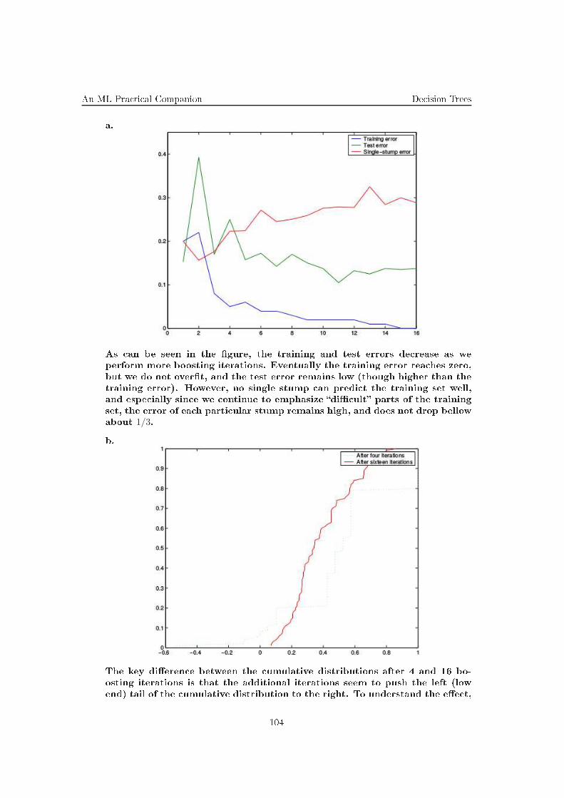
An ML Pra ti al Companion De ision Trees
a.
As an be seen in the gure, the training and test errors de rease as we
perform more boosting iterations. Eventually the training error rea hes zero,
but we do not overt, and the test error remains low (though higher than the
training error). However, no single stump an predi t the training set well,
and espe ially sin e we ontinue to emphasize di ult parts of the training
set, the error of ea h parti ular stump remains high, and does not drop bellow
about 1/3.
b.
The key dieren e between the umulative distributions after 4 and 16 bo-
osting iterations is that the additional iterations seem to push the left (low
end) tail of the umulative distribution to the right. To understand the ee t,
104

De ision Trees An ML Pra ti al Companion
note that the examples that are di ult to lassify have poor or negative
lassi ation margins and therefore dene the low end tail of the umulative
distribution. Additional boosting iterations on entrate on the di ult exam-
ples and ensure that their margins will improve. As the margins improve, the
left tail of the umulative distribution moves to the right, as we see in the
gure.
105

An ML Pra ti al Companion De ision Trees
37. (AdaBoost with logisti loss:
xxx studying the evolution of voting margins
xxx as a fun tion of boosting iterations)
• MIT, 2009 fall, Tommi Jaakkola, HW3, pr. 2.4
We have provided you with MatLab ode that you an run to test how Ada-
Boost works.
mod = boost(X,y,n omp) generates an ensemble (a ell array of n omp base lear-
ners) based on training examples X and labels y.load data.mat gives you X and y for a simple lassi ation task. You an
then generate the ensemble with any number of omponents (e.g., 50). The
ell array mod simply lists the base learners in the order in whi h they were
found. You an therefore plot the ensemble orresponding to the rst i
base learners by plot_de ision(mod(1:i),X,y), or individual base learners via
plot_de ision(modi,X,y).
plot_voting_margin(mod,X,y,th)helps you study how the voting margins hange
as a fun tion of boosting iterations. For example, the plot with th = 0 gives
the fra tion of orre tly lassied training points (voting margin > 0) as a
fun tion of boosting iterations. You an also plot the urves for multiple
thresholds at on e as in plot_voting_margin(mod,X,y,[0,0.05,0.1,0.5). Ex-
plain why some of these tend to in rease while others de rease as a fun tion
of boosting iterations. Why does the urve orresponding to th = 0.05 onti-
nue to in rease even after all the points are orre tly lassied?
Solution:
Let hm(x) =∑m
i=1 αihi(x) denote the ensemble lassier after m boosting ite-
rations, and let hm(x) =
∑mi=1 αihi(x)∑m
i=1 αibe its normalized version. Let f(τ,m)
denote the fra tion of training examples (xt, yt) with voting margin ythm(xt) =ythm(xt)∑m
i=1 αi> τ . From our plot, we noti e that f(τ,m) is in reasing with m (quite
roughly and not at all monotoni ally) for small values of τ , like τ = 0, 0.05, 0.1,but de reasing for large values of τ , like τ = 0.5. (The threshold at whi h the
transition o urs seems to be somewhere in the interval 0.115 > τ > 0.105.)
To explain this, onsider the boosting loss fun tion, Jm =∑n
t=1 L(yt hm(xt)),
whi h is de reasing in the voting margins ythm(xt). To minimize Jm, AdaBoost
will try to make all the voting margins yhm(xt) as positive as possible. As m
in reases,
∑mi=1 αi only grows, so a negative voting margin ythm(xt) < 0 only
be omes more ostly. So, after a su ient number of iterations, we know that
boosting will be able to lassify all points orre tly, and all points will have
positive voting margin. So, f(0,m) roughly in reases from 0.5 to 1, and stays
at 1 on e m is su iently large.
As m in reases even more, we should expe t that the minimum voting margin
mint yth(xt) ontinues to in rease. This is be ause there is little in entive to
make the larger ythm(xt) any more positive; it is more ee tive to make the
smaller ythm(xt) more positive. Using an argument similar to the one from
part a of this problem (MIT, 2009 fall, T. Jaakkola, HW3, pr. 2.1), we an
show that the examples whi h are barely orre t have larger weight (Wm(t))than the examples whi h are learly orre t, sin e dL(z) is larger near 0.
106

De ision Trees An ML Pra ti al Companion
However, our de ision stumps are fairly weak lassiers. If we want to per-
form better on some subset of points (namely, the ones with smaller margin),
we must ompromise on the rest (namely, the ones with larger margin). Thus,
what we get is that the minimum voting margin (whi h osts more) will be-
ome larger at the expense of the maximum voting margin (whi h osts less).
Similarly, f(τ, n) for a small threshold τ will in rease at the expense of f(τ, n)for a large τ .
A visual way to see this is to onsider a graph of the res aled loss fun tion
L((∑m
i=1 αi)τ) vs. the voting margin τ = ythm(xt). As the number of boosting
iterations in reases, the graph is ompressed along the horizontal axis (altho-
ugh in reasingly slowly). So to make Jm smaller, we must basi ally shift the
entire distribution of voting margins to the right as mu h as possible (tho-
ugh we an only do so in reasingly slowly). In doing this, we are for ed to
ompromise some of the points farthest to the right, moving them inward.
Thus, with more iterations, the distribution of margins narrows. Here, f(τ, n) an be related to the umulative density on the empiri al distribution of vo-
ting margins. So, f(τ, n) = P (margin > τ) for a small τ will in rease, while
1 − f(τ, n) = P (margin < τ) for large τ will also in rease (or at least be non-
de reasing).
[Caption: Voting Margins, 10-20 iterations.
107

An ML Pra ti al Companion De ision Trees
[Caption: Voting Margins, 40-80 iterations.
[Caption: Voting Margins, 200-400 iterations.
[Caption: Empiri al Distributions of Voting Margins.
108

De ision Trees An ML Pra ti al Companion
-0.5 0 0.5
-0.8
-0.6
-0.4
-0.2
0
0.2
0.4
0.6
0.8
-0.5 0 0.5
-0.8
-0.6
-0.4
-0.2
0
0.2
0.4
0.6
0.8
[Caption: De ision boundaries, 10-20 iterations.
-0.5 0 0.5
-0.8
-0.6
-0.4
-0.2
0
0.2
0.4
0.6
0.8
-0.5 0 0.5
-0.8
-0.6
-0.4
-0.2
0
0.2
0.4
0.6
0.8
[Caption: De ision boundaries, 40-80 iterations.
109

An ML Pra ti al Companion De ision Trees
-0.5 0 0.5
-0.8
-0.6
-0.4
-0.2
0
0.2
0.4
0.6
0.8
-0.5 0 0.5
-0.8
-0.6
-0.4
-0.2
0
0.2
0.4
0.6
0.8
[Caption: De ision boundaries, 200-400 iterations.
[Caption: De ision boundaries.
110
De ision Trees An ML Pra ti al Companion
38. (Liniear regression vs.
xxx AdaBoost using [weighted linear weak lassiers
xxx and mean square error as loss fun tion;
xxx ross-validation;
xxx appli ation on the Wine dataset)
• CMU, 2009 spring, Ziv Bar-Joseph, HW3, pr. 1
In this problem, you are going to ompare the performan e of a basi linear
lassier and its boosted version on the Wine dataset (available on our web-
site). The dataset, given in the le wine.mat, ontains the results of a hemi al
analysis of wines grown in the same region in Italy but derived from three
dierent ultivars. The analysis determined the quantities of 13 onstituents
found in ea h of the three types of wines. Note that when you are doing
ross-validation, you want to ensure that a ross all the folds the proportion
examples from ea h lass is roughly the same.
a. Implement a basi linear lassier using linear regression. All data points
are equally weighted.
A linear lassier is dened as:
f(x;β) = sign(β⊤ · x) =
−1 if β⊤ · x < 0;1 if β⊤ · x ≥ 0.
Your algorithm should minimize the lassi ation error dened as:
err(f) =
n∑
i=1
(yi − f(xi))2
4n
Note: The rst step for data prepro essing is to augment the data. In MatLab,
this an be done as:
X_new = [ones(size(X,1), 1) X;
Hint: You may want to use the MatLab fun tion fminsear h to get the optimal
solution for β.
Handin: Please turn in a MatLab sour e le linear_learn.m whi h takes in
two inputs data matrix x and label y, and returns a linear model. You may
have additional fun tions/les if you want.
b. Do 10-fold ross validation for the linear lassier. Report the average
training and test errors for all the folds.
Handin: Please turn in a MatLab sour e le v.m.
. Modify your algorithm in linear_learn.m to a ommodate weighted sam-
ples. Given the weight w for sample data X, what is the lassi ation error?
You may want to refer to part a. Please implement the weighted version of
the learning algorithm for the linear lassier.
Note originally the unweighted version ould be viewed as one with equal
weights 1/n.
Handin: Please turn in a MatLab sour e le linear_learn.m whi h takes in
three inputs data matrix x, label y and weights w, and returns a linear model.
You may have additional fun tions/les if you want. Note that your ode
111

An ML Pra ti al Companion De ision Trees
should have ba kward ompatibility it behaves like unweighted version if wis not given.
d. Implement AdaBoost for the linear lassifer using the re-weighting and
re-training idea. Refer to the le ture slides or to Ciortuz et al's ML exer ise
book for the AdaBoost algorithm.
Handin: Please turn in a MatLab sour e le adaBoost.m.
e. Do 10-fold ross-validation on the Wine dataset using AdaBoost with the
linear lassier as the weak learner, for 1 to 100 iterations. Plot the average
training and test errors for all the folds as a fun tion of the number of boosting
iterations. Also, draw horizontal lines orresponding to the training and test
errors for the linear lassier that you obtain in part b. Dis uss your results.
Handin: Please turn in a MatLab sour e le v ab.m. You may reuse fun tions
in part b.
Solution:
.
errw(f) =
n∑
i=1
wi(yi − f(xi))
2
4.
e. Sample plot:
0 20 40 60 80 1000
0.1
0.2
0.3
0.4
0.5
0.6
0.7
no of AdaBoost iterations
erro
r
train error lin classtest error lin classtrain error AdaBoosttest error AdaBoost
112

De ision Trees An ML Pra ti al Companion
39. (AdaBoost using Naive Bayes as weak lassier;
xxx appli ation on the US House of Representatives votes dataset)
• CMU, 2005 spring, C. Guestrin, T. Mit hell, HW2, pr. 1.2
Solution:
113

An ML Pra ti al Companion Support Ve tor Ma hines
5 Support Ve tor Ma hines
40. (An implementation of SVM using the quadprog MatLab fun tion;
xxx appli ation on dierent datasets from R2)
• · MIT, 2001 fall, Tommi Jaakkola, HW3, pr. 2
41. (Choosing an SVM kernel)
• · CMU, 2013 fall, A. Smola, B. Po zos, HW3, pr. 2
42. (An implementation of SVM using the quadprog MatLab fun tion;
xxx omparison with the per eptron;
xxx using SVMlight for digit re ognition)
• · MIT, 2006 fall, Tommi Jaakkola, HW1, se tion B
43. (ν-SVM: implementation using the quadprog MatLab fun tion;
xxx train and test it on a given dataset)
• · MIT, 2004 fall, Tommi Jaakkola, HW3, pr. 3.3
44. (Minimum En losing Ball (MEB) / Anomaly dete tion)
• · MIT, 2009 fall, Tommi Jaakkola, HW2, pr. 2. d
• CMU, 2017 fall, Nina Bal an, HW4, pr. 4.1
Let S = (x1, y1), . . . (xn, yn) be n labeled examples in Rdwith label set 1,−1.
Re all that the primal formulation of SVM is given by
Primal
minw∈Rd,ξ1,...ξn
‖w‖2 + Cn∑
i=1
ξi,
s.t. ∀i, yi 〈w,Xi〉 ≥ 1− ξi, ξi ≥ 0.
It an be proven (see ex. 21) that the primal problem an be rewritten as
the following equivalent problem in the Empiri al Risk Minimization (ERM)
framework
minw∈Rd
λ‖w‖22 +1
n
n∑
i=1
max(1− yi 〈w,Xi〉 , 0), (239)
where λ = 1nC .
We will now optimize the above un onstrained formulation of SVM using Sto-
hasti Sub-Gradient Des ent. In this problem you will be using a binary (two
114

Support Ve tor Ma hines An ML Pra ti al Companion
lass) version of mnist dataset. The data and ode template an be downloa-
ded from the lass website:
https://sites.google. om/site/10715advan edmlintro2017f/homework-exams.
The data folder has mnist2.mat le whi h ontains the train, test and valida-
tion datasets. The python folder has python ode template (and matlab folder
has the matlab ode template) whi h you will use for your implementation.
You an either use python or matlab for this programming question.
We slightly modify Equation (239) and use the following formulation in this
problem
minw∈Rd
λ
2‖w‖22 +
1
n
n∑
i=1
max(1 − yi 〈w,Xi〉 , 0).
This is only done to simplify al ulations. You will optimize this obje tive
using Sto hasti Sub-Gradient Des ent (SSGD).
727
This approa h is very sim-
ple and s ales well to large datasets.
728
In SSGD we randomly sample a
training data point in ea h iteration and update the weight ve tor by taking
a small step along the dire tion of negative sub-gradient of the loss.
729
The SSGD algorithm is given by
• Initialize the weight ve tor w = 0.
• For t = 1 . . . T
* Choose it ∈ 1, . . . n uniformly at random
* Set ηt =1λt .
* If yit 〈w,Xit〉 < 1 then:
Set w ← (1− ληt)w + ηtyitXit
* Else:
Set w ← (1− ληt)w
• Return w
Note that we don't onsider the bias/inter ept term in this problem.
a. Complete the train(w0, Xtrain, ytrain, T, lambda) fun tion in the svm.py
le (matlab users omplete the train.m le).
b. The fun tion train(w0, Xtrain, ytrain, T, lambda) runs the SSGD algo-
rithm, taking in an initial weight ve tor w0, matrix of ovariates Xtrain, a
ve tor of labels ytrain. T is the number of iterations of SSGD and lambda is
the hyper-parameter in the obje tive. It outputs the learned weight ve tor w.
. Run svm_run.py to perform training and see the performan e on training
and test sets.
d. Use validation dataset for pi king a good lambda(λ) from the set 1e3,
1e2, 1e1, 1, 0.1.
727
See Shai Shalev-Shwartz, Yoram Singer, Nathan Srebro, and Andrew Cotter. Pegasos: Primal estimated
sub-gradient solver for SVM. Mathemati al programming, 127(1):3-30, 2011.
728
To estimate optimal w, one an also optimize the dual formulation of this problem. Some of the popular
SVM solvers su h as LIBSVM solve the dual problem. Other fast approa hes for solving dual formulation on
large datasets use dual oordinate des ent.
729
Sub-gradient generalizes the notion of gradient to non-dierentiable fun tions.
115

An ML Pra ti al Companion Support Ve tor Ma hines
e. Report the a ura y numbers on train and test datasets obtained using the
best lambda, after running SSGD for 200 epo hs (i.e., T = 200 ∗ n). Generate
the training a ura y vs. training time and test a ura y vs training time
plots.
116

Arti ial Neural Networks An ML Pra ti al Companion
6 Arti ial Neural Networks
45. (Reµele neuronale: hestiuni de baz )
• MPI, 2005 spring, Jörg Rahnenfuhrer, Adrian Alexa, HW2, pr. 5
a. Simulate data by randomly drawing two-dimensional data points uniformly
distributed in [0, 1]2. The lass Y of a sample X = (X1, X2) is 1 if X1 +X2 > 1and −1 otherwise. You an add some noise to the data by using the rule
X1 + X2 > 1 + ε with ε ∼ N (0, 0.1). Use 100 samples for the training set (you
an use training data with or without noise).
b. Write a fun tion to train a per eptron for a two lass lassi ation problem.
A per eptron is a lassier whi h onstru ts a linear de ision boundary that
tries to separate the data into dierent lasses as best as possible. Se tion 4.5.1
in The Elements of Statisti al Learning book by Hastie, Tibshirani, Friedman
des ribes how the per eptron learning algorithm works.
. Write a fun tion to predi t the lass for new data points. Write a fun tion
that performs LOOCV (Leave-One-Out Cross-Validation) for your lassier.
Use these fun tions to estimate the train error and the the predi tion er-
ror. Generate a test set of 1000 samples and ompute the test error of your
lassier.
d. Use the data generator xor.data() from the tutorial homepage to generate
a new training ( a. 100 samples) and test set ( a. 1000 samples). Train the
per eptron on this data. Report the train and test errors. Plot the test
samples to see how they are lassied by the per eptron.
e. Comment your ndings. Is the per eptron able to learn the XOR data?
What is the main dieren e between the data generated in part a and the
data from part d?
f. Use the nnet R pa kage to train a neural network for the XOR data. The
nnet() fun tion is tting a neural network. Use the predi t() fun tion to asses
the train and test errors.
h. Vary the number of units in the hidden layer and report the train and test
errors. We have seen at part e that a per eptron, a neural network with no
unit in the hidden layer an not orre tly lassify the XOR data. Argue whi h
is the minimal number of units in the hidden layer that a neural network must
have to orre tly lassify the XOR data. Train su h a network and report the
train, predi tion and test errors.
117

An ML Pra ti al Companion Arti ial Neural Networks
46. (The Per eptron algorithm:
xxx spam identi ation)
• New York University, 2016 spring, David Sontag, HW1
In this problem set you will implement the Per eptron algorithm and apply
it to the problem of e-mail spam lassi ation.
Instru tions. You may use the programming language of your hoi e (we
re ommend Python, and using matplotlib for plotting). However, you are
not permitted to use or referen e any ma hine learning ode or pa kages not
written by yourself.
Data les. We have provided you with two les: spam train.txt, and spam
test.txt. Ea h row of the data les orresponds to a single email. The rst
olumn gives the label (1=spam, 0=not spam).
Pre-pro essing. The dataset in luded for this exer ise is based on a subset of
the SpamAssassin Publi Corpus. Figure 1 shows a sample email that ontains
a URL, an email address (at the end), numbers, and dollar amounts. While
many emails would ontain similar types of entities (e.g., numbers, other
URLs, or other email addresses), the spe i entities (e.g., the spe i URL or
spe i dollar amount) will be dierent in almost every email. Therefore, one
method often employed in pro essing emails is to normalize these values,
so that all URLs are treated the same, all numbers are treated the same,
et . For example, we ould repla e ea h URL in the email with the unique
string httpaddr to indi ate that a URL was present. This has the ee t
of letting the spam lassier make a lassi ation de ision based on whether
any URL was present, rather than whether a spe i URL was present. This
typi ally improves the performan e of a spam lassier, sin e spammers often
randomize the URLs, and thus the odds of seeing any parti ular URL again
in a new pie e of spam is very small.
We have already implemented the following email prepro essing steps: lower-
asing; removal of HTML tags; normalization of URLs, e-mail addresses, and
numbers. In addition, words are redu ed to their stemmed form. For example,
dis ount, dis ounts, dis ounted and dis ounting are all repla ed with
dis oun. Finally, we removed all non-words and pun tuation. The result of
these prepro essing steps is shown in Figure 2.
Figure 1: Sample e-mail in SpamAssassin orpus before pre-pro essing.
> Anyone knows how mu h it osts to host a web portal?
> Well, it depends on how many visitors youre expe ting. This an be
anywhere from less than 10 bu ks a month to a ouple of $100. You sho-
uld he kout http://www.ra kspa e. om/ or perhaps Amazon EC2 if youre
running something big.
To unsubs ribe yourself from this mailing list, send an email to: groupname-
unsubs ribeegroups. om.
Figure 2: Pre-pro essed version of the sample e-mail from Figure 1.
anyon know how mu h it ost to host a web portal well it depend on how mani
visitor your expe t thi an be anywher from less than number bu k a month
to a oupl of dollarnumb you should he kout httpaddr or perhap amazon
e numb if your run someth big to unsubs rib yourself from thi mail list send
an email to emailaddr
118

Arti ial Neural Networks An ML Pra ti al Companion
a. This problem set will involve your implementing several variants of the
Per eptron algorithm. Before you an build these models and measure their
performan e, split your training data (i.e. spam_train.txt) into a training
and validation set, putting the last 1000 emails into the validation set. Thus,
you will have a new training set with 4000 emails and a validation set with
1000 emails. You will not use spam_test.txt until problem j. Explain why
measuring the performan e of your nal lassier would be problemati had
you not reated this validation set.
b. Transform all of the data into feature ve tors. Build a vo abulary list using
only the 4000 e-mail training set by nding all words that o ur a ross the
training set. Note that we assume that the data in the validation and test
sets is ompletely unseen when we train our model, and thus we do not use
any information ontained in them. Ignore all words that appear in fewer
than X = 30 e-mails of the 4000 e-mail training set this is both a means of
preventing overtting and of improving s alability. For ea h email, transform
it into a feature ve tor x where the ith entry, xi, is 1 if the ith word in the
vo abulary o urs in the email, and 0 otherwise.
. Implement the fun tions per eptron_train(data) and per eptron_test(w,
data).
The fun tion per eptron_train(data) trains a per eptron lassier using the
examples provided to the fun tion, and should return w, k, and iter, the nal lassi ation ve tor, the number of updates (mistakes) performed, and the
number of passes through the data, respe tively. You may assume that the
input data provided to your fun tion is linearly separable (so the stopping
riterion should be that all points are orre tly lassied). For the orner
ase of w · x = 0, predi t the +1 (spam) lass.
For this exer ise, you do not need to add a bias feature to the feature ve tor (it
turns out not to improve lassi ation a ura y, possibly be ause a frequently
o urring word already serves this purpose). Your implementation should
y le through the data points in the order as given in the data les (rather
than randomizing), so that results are onsistent for grading purposes.
The fun tion per eptron_test(w, data) should take as input the weight ve tor
w (the lassi ation ve tor to be used) and a set of examples. The fun tion
should return the test error, i.e. the fra tion of examples that are mis lassied
by w.
d. Train the linear lassier using your training set. How many mistakes
are made before the algorithm terminates? Test your implementation of
per eptron_test by running it with the learned parameters and the training
data, making sure that the training error is zero. Next, lassify the emails in
your validation set. What is the validation error?
e. To better understand how the spam lassier works, we an inspe t the
parameters to see whi h words the lassier thinks are the most predi tive of
spam. Using the vo abulary list together with the parameters learned in the
previous question, output the 15 words with the most positive weights. What
are they? Whi h 15 words have the most negative weights?
f. Implement the averaged per eptron algorithm, whi h is the same as your
urrent implementation but whi h, rather than returning the nal weight ve -
tor, returns the average of all weight ve tors onsidered during the algorithm
119

An ML Pra ti al Companion Arti ial Neural Networks
(in luding examples where no mistake was made). Averaging redu es the va-
rian e between the dierent ve tors, and is a powerful means of preventing
the learning algorithm from overtting (serving as a type of regularization).
g. One should expe t that the test error de reases as the amount of training
data in reases. Using only the rst N rows of your training data, run both the
per eptron and the averaged per eptron algorithms on this smaller training
set and evaluate the orresponding validation error (using all of the validation
data). Do this for N = 100, 200, 400, 800, 2000, 4000, and reate a plot of the
validation error of both algorithms as a fun tion of N .
h. Also for N = 100, 200, 400, 800, 2000, 4000, reate a plot of the number of per- eptron iterations as a fun tion of N , where by iteration we mean a omplete
pass through the training data. As the amount of training data in reases, the
margin of the training set de reases, whi h generally leads to an in rease in
the number of iterations per eptron takes to onverge (although it need not
be monotoni ).
i. One onsequen e of this is that the later iterations typi ally perform updates
on only a small subset of the data points, whi h an ontribute to overtting.
A way to solve this is to ontrol the maximum number of iterations of the
per eptron algorithm. Add an argument to both the per eptron and averaged
per eptron algorithms that ontrols the maximum number of passes over the
data.
j. Congratulations, you now understand various properties of the per eptron
algorithm. Try various ongurations of the algorithms on your own using all
4000 training points, and nd a good onguration having a low error on your
validation set. In parti ular, try hanging the hoi e of per eptron algorithm
and the maximum number of iterations. You ould additionally hange Xfrom question b (this is optional). Report the validation error for several of
the ongurations that you tried; whi h onguration works best?
You are ready to train on the full training set, and see if it works on omple-
tely new data. Combine the training set and the validation set (i.e. use all
of spam_train.txt) and learn using the best of the ongurations previously
found. You do not need to rebuild the vo abulary when re-training on the
train+validate set.What is the error on the test set (i.e., now you nally use spam test.txt)?
Note: This problem set is based partly on an assignment developed by Andrew
Ng of Stanford University and Coursera.
120

Arti ial Neural Networks An ML Pra ti al Companion
47. (The ba kpropagation algorithm:
xxx appli ation on the Breast Can er dataset)
• MPI, 2005 spring, Jörg Rahnenfuhrer, Adrian Alexa, HW2, pr. 6
Download the breast an er data set breast an er.zip from the tutorial ho-
mepage. The data are des ribed in Mike West et al.: Predi ting the lini-
al status of human breast an er by using gene expression proles, PNAS
98(20):11462-11467, 2001. The le ontains expression proles of 46 patients
from two dierent lasses: 23 patients are estrogen re eptor positive (ER+)
and 23 are estrogen re eptor negative (ER-). For every patient, the expres-
sion values of 7129 genes were measured. Use the nnet R pa kage to train a
neural network.
a. Load breast an er.Rdata and apply summary() to get an overview of this
data obje t: breast an er$x ontains the expression data and breast an er$y
the lass labels. Reformat the data by transposing the gene expression matrix
and renaming the lasses ER+, ER− to +1,−1.b. Train a Neural Network using the nnet() fun tion. Che k if the inputs are
standardized (mean zero and standard deviation one) and if this is not the
ase, standardize them.
. Apply the fun tion predi t() to the training data and al ulate the trai-
ning error. Perform a LOOCV to estimate the predi tion error (you must
implement by yourself the ross validation pro edure).
d. Predi t the lasses of the three new patients (newpatients). The true lass
labels are stored in (true lasses). Are they orre tly lassied?
e. Try dierent parameters in the nnet() fun tion (the number of units in the
hidden layer, the weights, the a tivation fun tion, the weight de ay parame-
ter, et .) and report the parameters for whi h you obtained the best result.
Comment the way the parameters ae t the performan e of the network.
121

An ML Pra ti al Companion Arti ial Neural Networks
48. (Arti ial neural networks:
xxx Digit lassi ation ompetition)
• CMU, 2014 fall, William Cohen, Ziv Bar-Joseph, HW3
In this se tion, you are asked to onstru t a neural network using a dataset
in real world. The training samples and training labels are provided in the
handout folder. Ea h sample is a 28×28 gray s ale image. Ea h pixel (feature)
is a real value between 0 and 1 denoting the pixel intensity. Ea h label is a
integer from 0 to 9 whi h orresponds to the digit in the image.
A. Getting Started
Getting Familiar with Data
As mentioned above, ea h sample is an image with 784 pixels. Load the data
using the following ommand:
load(`digits.mat')
Visualize an image using the following ommand:
imshow(ve 2mat(XTrain(i,:),28)')
where X ∈ Rn×784
is the training samples; i is the row index of a training
sample.
Neural Network Stru ture
In this ompetition, you are free to use any neural network stru ture. A simple
feed forward neural network with one hidden layer is shown in Figure... . The
input layer has a bias neuron and 784 neurons with ea h orresponding to one
pixel in the image. The output layer has 10 neurons with ea h representing
the probability of ea h digit given the image. You need to de ide the size of
the hidden layer.
Code Stru ture
You should implement your training algorithm (typi ally the forward pro-
pagation and ba k propagation) in train_ann.m and testing algorithm (using
trained weights to predi t labels) in test_ann.m. In your training algorithm,
you need to store your initial and nal weights into a mat le. In the simple
example below, two weight matri es Wih and Who are stored into weights.mat:
save(`weights.mat',`Wih',`Who');
Be sure your test ann.m runs fast enough. It is always good to ve torize your
ode in Matlab.
Separating Data
Digits.mat ontains 3000 instan es whi h you used in previous se tion. The
number of instan es are pretty balan ed for ea h digit so you do not need to
worry about skewness of the data. However, you need to handle the overtting
problem. Neural networks are very powerful models whi h are apable to
express extremely ompli ated fun tions but very prone to overt.
The standard approa h for building a model on a dataset an be des ribed as
follows:
• Divide your data into three sets: a training set, a validation set, a test
set. You an use any sizes for three sets as long as they are reasonable
(e.g. 60%, 20%, 20%). You an also ombine the training set and the
validation set and do k-fold ross-validation. Make sure to have balan ed
numbers of instan es for ea h lass in every set.
122

Arti ial Neural Networks An ML Pra ti al Companion
• Train your model on the training set and tune your parameters on the
validation set. By tuning the parameters (e.g. number of neurons, num-
ber of layers, regularization, et ...) to a hieve maximum performan e on
the validation set, the overtting problems an be somehow alleviated.
The following webpage provides some reasonable ranges for parameter
sele tion:
http://en.wikibooks.org/wiki/Artifi ial_Neural_Networks/Neural_Network_Basi s
• If the training a ura y is mu h higher than validation a ura y, the
model is overtting; if the training a ura y and validation a ura y are
both very low, the model is undertting; if both a ura ies are high but
test a ura y is low, the model should be dis arded.
B. Bag of Tri ks for Training a Neural Network
Overtting vs Undertting
This is related to the model sele tion problem [that we are going to dis uss
later in this ourse. It is extremely important to determine whether the
model is overtting or undertting. The table below shows several general
approa hes to dis over and alleviate these problems:
Overt Undert
Performan e Training a ura y mu h Both a ura ies are low
higher than validation a ura y
Data Need more data If two a ura ies are lose,
no need for extra data
Model Use a simpler model Use a more ompli ated model
Features Redu e number of features In rease number of features
Regularization In rease regularization Redu e regularization
There are other ways to redu e overtting and undertting problems parti-
ular for neural networks, and we will dis uss them in other tri ks.
Early Stopping
A ommon reason for overtting is that the neural net
onverges to a bad minimum. In the nearby gure, the
solid line orresponds to the error surfa e of a trained
neural net while the dash line orresponds to the true
model. Point A is very likely to be a bad minimum sin e
the narrow valley is very likely to be aused by over-
tting to training data. Point B is a better minimum
sin e it is mu h smoother and more likely be the true
minimum.
To alleviate overtting, we an stop the
training pro ess before the network on-
verges. In the nearby gure, if the trai-
ning pro edure stops when network a hie-
ves best performan e on validation set, the
overtting problem is somehow redu ed.
However, in reality, the error surfa e may
be very irregular. A ommon approa h is
to store the weights after ea h epo h until
the network onverges. Pi k the weights
that performs well on the validation set.
123

An ML Pra ti al Companion Arti ial Neural Networks
Multiple Initialization
When training a neural net, people typi ally initialize weights to very small
numbers (e.g. a Gaussian random number with 0 mean and 0.005 varian e).
This pro ess is alled symmetry breaking. If all the weights are initialized to
zero, all the neurons will end up learning the same feature. Sin e the error
surfa e of neural networks is highly non- onvex, dierent weight initializations
will potentially onverge to dierent minima. You should store the initialized
weights into ini weights.mat.
Momentum
Another way to es ape from a bad minimum is adding a momentum term into
weight updates. The momentum term is α∆W (n − 1) in equation 240, where
n denotes the number of epo hs. By adding this term to the update rule, the
weights will have some han e to es ape from minimum. You an set initial
momentum to zero.
∆W (n) = ∇WJ(W, b) + α∆W (n− 1) (240)
The intuition behind this approa h is the
same as this term in physi s systems. In
the nearby gure, assume weights grow po-
sitively during training, without the mo-
mentum term, the neural net will onverge
to point A. If we add the momentum term,
the weights may jump over the barrier and
onverge to a better minimum at point B.
Bat h Gradient Des ent vs Sto hasti Gradient Des ent
As we dis ussed in the le tures, given enough memory spa e, bat h gradient
des ent usually onverges faster than sto hasti gradient des ent. However,
if working on a large dataset (whi h ex eeds the apa ity of memory spa e),
sto hasti gradient des ent is preferred be ause it uses memory spa e more
e iently. Mini-bat h is a ompromise of these two approa hes.
Change A tivation Fun tion
As we mentioned in the theoreti al questions, there are many other a tivation
fun tions other than logisti sigmoid a tivation, su h as (but not limited to)
re tied linear fun tion, ar tangent fun tion, hyperboli fun tion, Gaussian
fun tion, polynomial fun tion and softmax fun tion. Ea h a tivation has die-
rent expressiveness and omputation omplexity. The sele tion of a tivation
fun tion is problem dependent. Make sure to al ulate the gradients orre tly
before implementing them.
Pre-training
Autoen oder is a unsupervised learning algorithm to automati ally learn fe-
atures from unlabeled data. It has a neural network stru ture with its input
being exa tly the same as output. From input layer to hidden layer(s), the
features are abstra ted to a lower dimensional spa e. Form hidden layer(s)
to output layer, the features are re onstru ted. If the a tivation is linear, the
124

Arti ial Neural Networks An ML Pra ti al Companion
network performs very similar to Prin iple Component Analysis (PCA). After
training an autoen oder, you should keep the weights from input layer and
hidden layers, and build a lassier on top of hidden layer(s). For implementa-
tion details, please refer to Andrew Ng's s294A ourse handout at Stanford:
http://web.stanford.edu/ lass/ s294a/sparseAutoen oder_2011new.pdf
More Neurons vs Less Neurons
As mentioned above, we should use more ompli ated models for undertting
ases, and simpler models for overtting ases. In terms of neural networks,
more neurons mean higher omplexity. You should pi k the size of hidden
layer based on training a ura y and validation a ura y.
More Layers?
Adding one or two hidden layers may be useful, sin e the model expressiveness
grows exponentially with extra hidden layers. You an apply the same ba k
propagation te hnique as training a single hidden layer network. However,
if you use even more layers (e.g. 10 layers), you are denitely going to get
extremely bad results. Any networks with more than one hidden layer is
alled a deep network. Large deep network en ounters the vanishing gradient
problem using the standard ba k propagation algorithm (ex ept onvolutional
neural nets). If you are not familiar with onvolutional neural nets, or training
sta ks of Restri ted Boltzmann Ma hines, you should sti k with a few hidden
layers.
Sparsity
Sparsity on weights (LASSO penalty) for es neurons to learn lo alized infor-
mation. Sparsity on a tivations (KL-divergen e penalty) for es neurons to
learn ompli ated features.
Other Te hniques
All the tri ks above an be applied to both shallow networks and deep ne-
tworks. If you are interested, there are other tri ks whi h an be applied to
(usually deep) neural networks:
• Dropout
• Model Averaging
[You an nd these information in oursera le tures provided by Georey
Hinton.
125

An ML Pra ti al Companion Arti ial Neural Networks
49. (Per eptronul Rosenblatt:
xxx al ul mistake bounds;
xxx al ul margini; omparaµie u SVM)
• MIT, 2006 fall, Tommy Jaakkola, HW1, pr. 1-2
Implement a Per eptron lassier in MATLAB. Start by implementing the
following fun tions:
− a fun tion per eptron_train(X, y) where X and y are n × d and n × 1 ma-
tri es respe tively. This fun tion trains a Per eptron lassier on a training
set of n examples, ea h of whi h is a d-dimensional ve tor. The labels for the
examples are in y and are 1 or −1. The fun tion should return [theta, k, the
nal lassi ation ve tor and the number of updates performed, respe tively.
You may assume that the input data provided to your fun tion is linearly
separable. Training the Per eptron should stop when it makes no errors at
all on the training data.
− a fun tion per eptron_test(theta, X_test, y_test) where theta is the las-
si ation ve tor to be used. X_test and y_test are m × d and m × 1 matri es
respe tively, orresponding to m test examples and their true labels. The
fun tion should return test err, the fra tion of test examples whi h were
mis lassied.
For this problem, we have provided you two ustom- reated datasets. The
dimension d of both the datasets is 2, for ease of plotting and visualization.
a. Load data using the load p1 a s ript and train your Per eptron lassier on
it. Using the fun tion per eptron_test, ensure that your lassier makes no
errors on the training data. What is the angle between theta and the ve tor
(1, 0)⊤? What is the number of updates ka required before the Per eptron
algorithm onverges?
b. Repeat the above steps for data loaded from s ript load_p1_b. What is
the angle between theta and the ve tor (1, 0)⊤ now? What is the number of
updates kb now?
. For parts a and b, ompute the geometri margins, γageom
and γbgeom
, of your
lassiers with respe t to their orresponding training datasets. Re all that
the distan e of a point xt from the θ⊤x = 0 is |θ⊤xt
||θ|| |.
d. For parts a and b, ompute Ra and Rb, respe tively. Re all that for any
dataset χ, R = max||x|||x ∈ χ.
e. Plot the data (as points in the X-Y plane) from part a, along with de ision
boundary that your Per eptron lassier omputed. Create another plot,
this time using data from part b and the orresponding de ision boundary.
Your plots should learly indi ate the lass of ea h point (e.g., by hoosing
dierent olors or symbols to mark the points from the two lasses). We have
a provided a MATLAB fun tion plot_points_and_ lassifier whi h you may
nd useful.
Implement an SVM lassier in MATLAB, arranged like the [above Per ep-
tron algorithm, with fun tions svm_train(X, y) and svm_test(theta, X test,
y test). Again, in lude a printout of your ode for these fun tions.
126

Arti ial Neural Networks An ML Pra ti al Companion
Hint: Use the built-in quadrati program solver quadprog(H, f, A, b) whi h
solves the quadrati program: min1
2x⊤Hx+f⊤x subje t to the onstraint Ax ≤
b.
f. Try the SVM on the two datasets from parts a and b. How dierent are the
values of theta from values the Per eptron a hieved? To do this omparison,
should you ompute the dieren e between two ve tors or something else?
g. For the de ision boundaries omputed by SVM, ompute the orresponding
geometri margins (as in part c). How do the margins a hieved using the SVM
ompare with those a hieved by using the Per eptron?
127

An ML Pra ti al Companion Arti ial Neural Networks
50. (Kernelized per eptron)
• MIT, 2006 fall, Tommy Jaakkola, HW2, pr. 3
Most linear lassiers an be turned into a kernel form. We will fo us here
on the simple per eptron algorithm and use the resulting kernel version to
lassify data that are not linearly separable.
a. First we need to turn the per eptron algorithm into a form that involves
only inner produ ts between the feature ve tors. We will fo us on hyper-
planes through origin in the feature spa e (any oset omponent [LC: is as-
sumed to be provided as part of the feature ve tors). The mistake driven
parameter updates are: θ ← θ + ytφ(xt) if ytθ⊤φ(xt) ≤ 0, where θ = 0 initially.
Show that we an rewrite the per eptron updates in terms of simple additive
updates on the dis riminant fun tion f(x) = θ⊤φ(x):
f(x)← f(x) + ytK(xt, x) if ytf(xt) ≤ 0,
where K(xt, x) = φ(xt)⊤φ(x) is any kernel fun tion and f(x) = 0 initially.
b. We an repla e K(xt, x) with any kernel fun tion of our hoi e su h as
the radial basis kernel where the orresponding feature mapping is innite
dimensional. Show that there always is a separating hyperplane if we use the
radial basis kernel. hint: Use the answers to the previous exer ise in this
homework (MIT, 2006 fall, Tommy Jaakkola, HW2, pr. 2).
. With the radial basis kernel we an therefore on lude that the per eptron
algorithm will onverge (stop updating) after a nite number of steps for any
dataset with distin t points. The resulting fun tion an therefore be written
as
f(x) =
n∑
i=1
wiyiK(xi, x)
where wi is the number of times we made a mistake on example xi. Most of
wi's are exa tly zero so our fun tion won't be di ult to handle. The same
form holds for any kernel ex ept that we an no longer tell whether the wi's
remain bounded (problem is separable with the hosen kernel). Implement
the new kernel per eptron algorithm in MATLAB using a radial basis and
polynomial kernels. The data and helpful s ripts are provided in...
Dene fun tions
alpha = train_kernel_per eptron(X, y, kernel_type) and
f = dis riminant_fun tion(alpha, X, kernel_type, X_test)
to train the pereptron and to evaluate the resulting f(x) for test examples,
respe tively.
d. Load the data using the load_p3_a s ript. When you use a polynomial
kernel to separate the lasses, what degree polynomials do you need? Draw the
de ision boundary (see the provided s ript plot_de _boundary) for the lowest-
degree polynomial kernel that separates the data. Repeat the pro ess for the
radial basis kernel. Briey dis uss your observations.
128

Arti ial Neural Networks An ML Pra ti al Companion
51. (Convolutional neural networks:
xxx implementation and appli ation on the MNIST dataset)
• CMU, 2016 fall, N. Bal an, M. Gormley, HW6
xxx CMU, 2016 spring, W. Cohen, N. Bal an, HW7
In this assignment, we are going to implement a Convolution Neural Network
(CNN) to lassify hand written digits of MNIST
730
data. Sin e the breakthro-
ugh of CNNs on ImageNet lassi ation (A. Krizhevsky, I. Sutskever, G. E.
Hinton, 2012), CNNs have been widely applied and a hieved the state the art
of results in many areas of omputer vision. The re ent AI programs that an
beat humans in playing Atari game (V. Mnih, K. Kavuk uoglu et al, 2015)
and Go (D. Silver, A. Huang et al, 2016) also used CNNs in their models.
We are going to implement the earliest CNN model, LeNet (Y. LeCun, L.
Bottou, Y. Bengio, P. Haner, 1998), that was su essfully applied to lassify
hand written digits. You will get familiar with the workow needed to build
a neural network model after this assignment.
The Stanford CNN ourse
731
and UFLDL
732
material are ex ellent for begin-
ners to read. You are en ouraged to read some of them before doing this
assignment.
A. We begin by introdu ing the basi stru ture and building blo ks of CNNs.
CNNs are made up of layers that have learnable parameters in luding weights
and bias. Ea h layer takes the output from previous layer, performs some
operations and produ es an output. The nal layer is typi ally a softmax
fun tion whi h outputs the probability of the input being in dierent lasses.
We optimize an obje tive fun tion over the parameters of all the layers and
then use sto hasti gradient des ent (SGD) to update the parameters to train
a model.
Depending on the operation in the layers, we an divide the layers into fol-
lowing types:
1. Inner produ t layer (fully onne ted layer)
As the name suggests, every output neuron of inner produ t layer has full
onne tion to the input neurons. The output is the multipli ation of the
input with a weight matrix plus a bias oset, i.e.:
f(x) = Wx+ b. (241)
This is simply a linear transformation of the input. The weight parameter Wand bias parameter b are learnable in this layer. The input x is d dimensional
olumn ve tor, and W is a d× n matrix and b is n dimensional olumn ve tor.
2.A tivation layer
We add nonlinear a tivation fun tions after the inner produ t layers to model
the non-linearity of real data. Here are some of the popular hoi es for non-
linear a tivation:
730
http://yann.le un. om/exdb/mnist/
731
http:// s231n.github.io/
732
http://ufldl.stanford.edu/tutorial/
129
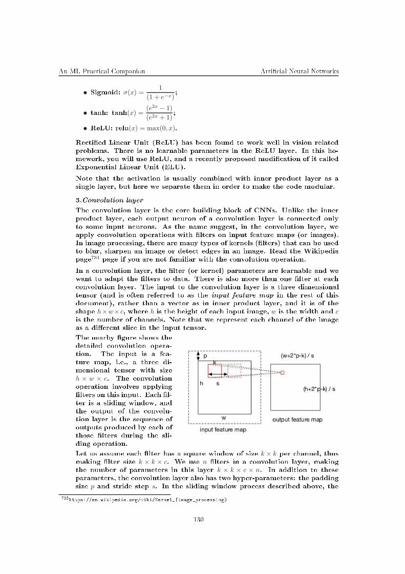
An ML Pra ti al Companion Arti ial Neural Networks
• Sigmoid: σ(x) =1
(1 + e−x);
• tanh: tanh(x) =(e2x − 1)
(e2x + 1);
• ReLU: relu(x) = max(0, x).
Re tied Linear Unit (ReLU) has been found to work well in vision related
problems. There is no learnable parameters in the ReLU layer. In this ho-
mework, you will use ReLU, and a re ently proposed modi ation of it alled
Exponential Linear Unit (ELU).
Note that the a tivation is usually ombined with inner produ t layer as a
single layer, but here we separate them in order to make the ode modular.
3.Convolution layer
The onvolution layer is the ore building blo k of CNNs. Unlike the inner
produ t layer, ea h output neuron of a onvolution layer is onne ted only
to some input neurons. As the name suggest, in the onvolution layer, we
apply onvolution operations with lters on input feature maps (or images).
In image pro essing, there are many types of kernels (lters) that an be used
to blur, sharpen an image or dete t edges in an image. Read the Wikipedia
page
733
page if you are not familiar with the onvolution operation.
In a onvolution layer, the lter (or kernel) parameters are learnable and we
want to adapt the lters to data. There is also more than one lter at ea h
onvolution layer. The input to the onvolution layer is a three dimensional
tensor (and is often referred to as the input feature map in the rest of this
do ument), rather than a ve tor as in inner produ t layer, and it is of the
shape h×w× c, where h is the height of ea h input image, w is the width and cis the number of hannels. Note that we represent ea h hannel of the image
as a dierent sli e in the input tensor.
The nearby gure shows the
detailed onvolution opera-
tion. The input is a fea-
ture map, i.e., a three di-
mensional tensor with size
h × w × c. The onvolution
operation involves applying
lters on this input. Ea h l-
ter is a sliding window, and
the output of the onvolu-
tion layer is the sequen e of
outputs produ ed by ea h of
those lters during the sli-
ding operation.
Let us assume ea h lter has a square window of size k × k per hannel, thus
making lter size k × k × c. We use n lters in a onvolution layer, making
the number of parameters in this layer k × k × c × n. In addition to these
parameters, the onvolution layer also has two hyper-parameters: the padding
size p and stride step s. In the sliding window pro ess des ribed above, the
733
https://en.wikipedia.org/wiki/Kernel_(image_pro essing)
130

Arti ial Neural Networks An ML Pra ti al Companion
output from ea h lter is a fun tion of a neighborhood of input feature map.
Sin e the edges have fewer neighbors, applying a lter dire tly is not feasible.
To avoid this problem, inputs are typi ally padded (with zeros) on all sides,
ee tively making the the height and width of the padded input h + 2p and
w + 2p respe tively, where p is the size of padding. Stride (s) is the step size
of onvolution operation.
As the above gure shows, the red square on the left is a lter applied lo ally
on the input feature map. We multiply the lter weights (of size k×k×c) witha lo al region of the input feature map and then sum the produ t to get the
output feature map. Hen e, the rst two dimensions of output feature map is
[(h+ 2p− k)/s+ 1]× [(w + 2p− k)/s+ 1]. Sin e we have n lters in a onvolution
layer, the output feature map is of size [(h+2p−k)/s+1]× [(w+2p−k)/s+1]×n.
For more details about the onvolutional layer, see Stanford's ourse on CNNs
for visual re ognition.
734
4. Pooling layer
It is ommon to use pooling layers after onvolutional layers to redu e the spa-
tial size of feature maps. Pooling layers are also alled down-sample layers,
and perform an aggregation operation on the output of a onvolution layer.
Like the onvolution layer, the pooling operation also a ts lo ally on the fea-
ture maps. A popular kind of pooling is max-pooling, and it simply involves
omputing the maximum value within ea h feature window. This allows us
to extra t more salient feature maps and redu e the number of parameters
of CNNs to redu e over-tting. Pooling is typi ally applied independently
within ea h hannel of the input feature map.
5. Loss layer
For lassi ation task, we use a softmax fun tion to assign probability to ea h
lass given the input feature map:
p = softmax(Wx+ b). (242)
In training, we know the label given the input image, hen e, we want to
minimize the negative log probability of the given label:
l = − log(pj), (243)
where j is the label of the input. This is the obje tive fun tion we would like
optimize.
B. LeNet Having introdu ed the building omponents of CNNs, we now in-
trodu e the ar hite ture of LeNet.
Layer Type Conguration
Input size: 28× 28× 1Convolution k = 5, s = 1, p = 0, n = 20Pooling MAX, k = 2, s = 2, p = 0Convolution k = 5, s = 1, p = 0, n = 50Pooling MAX, k = 2, s = 2, p = 0IP n = 500ReLU
Loss
734
http:// s231n.github.io/ onvolutional-networks/
131

An ML Pra ti al Companion Arti ial Neural Networks
The ar hite ture of LeNet is shown in Table. 51. The name of the layer type
explains itself. LeNet is omposed of interleaving of onvolution layers and
pooling layers, followed by an inner produ t layer and nally a loss layer. This
is the typi al stru ture of CNNs.
132

Clustering An ML Pra ti al Companion
7 Clustering
52. (Hierar hi al lustering and K-means:
xxx appli ation on the yeast gene expression dataset)
• CMU, 2010 fall, Carlos Guestrin, HW4, pr. 3
Now that you have been in the Ma hine Learning lass for almost 2 months,
you have earned the rst rank of number run hing ma hine learner. Re ently,
you landed a job at the Nexus lab of Cranberry Melon University. Your rst
task at the lab is to analyze gene expression data (whi h measures the levels
of genes in ells) for some mysterious yeast ells. You are given two datasets:
a set of 12 yeast genes in yeast1.txt, and a set of 52 yeast genes in yeast2.txt.
You are told that these genes are riti al to solve the myster of these ells.
You just learnt lustering so you hope that this te hnique ould help you
pinpoint groups of genes that may explain the mystery. The format of the
les is as follows: the rst olumn lists an identier for ea h gene, the se ond
olumn lists a ommon name for the gene and a des ription of its fun tion
and the remaining olumns list expression values for the gene under various
onditions.
Your program should not use the gene des riptions when performing luste-
ring. However, it may be informative to see them in the output. These genes
belong to four ategories for whi h the genes in ea h should exhibit fairly
similar expression proles.
a. Implement the agglomerative hierar hi al lustering that you learnt in
lass. You annot use Matlab's linkage fun tion or any fun tion that om-
putes the linkage/tree. Use the Eu lidean distan e as the distan e between
expression ve tors of two genes. You only need to implement single linkage
lustering.
Your output should be a tab-delimited text le. Ea h line of the le des ribes
one internal node of the tree: the rst olumn is the identier of the rst node,
the se ond olumn is the identier of the se ond node, and the third olumn
is the linkage between the two nodes. Note that ea h agglomeration o urs
at a greater distan e between lusters than the previous agglomeration. For
leaf nodes, use the gene name as the identier and for internal nodes, use the
line number where the node was des ribed.
To test your method, the output using single linkage on the small set is pro-
vided in single1.txt:
YKL145W YGL048C 2.391171
YFL018C YGR183C 3.383814
YLR038C YLR395C 3.461156
3 2 4.144297
4 1 4.163976
YOR369C YPL090C 4.328152
5 YDL066W 4.463093
6 YOR182C 4.837613
7 YPR001W 5.246656
9 YGR270W 5.373565
10 8 6.050942
133

An ML Pra ti al Companion Clustering
Submit the ode and following output le single2.txt for single linkage lus-
tering of the big set.
b. From the output tree, we an get K lusters by utting the tree at a er-
tain threshold d. That is any internal nodes with the linkage greater than
d are dis arded. The genes are lustered a ording to the remaining nodes.
Implement a fun tion that output K lusters given the value K. Your fun -
tion should nd the threshold d automati ally from the onstru ted tree. The
output le lists the genes belong to ea h luster. Ea h line of the le ontains
two olumns: the gene identier (the rst olumn in the original input le)
and the des ription (the se ond olumn.) A blank line is used to separated the
lusters. For the tree in single1.txt, to get 2 lusters, we use the threshold
6.01 to ut the tree. The le 2single1.txt is an example output le as shown
here:
YPL090C RPS6A PROTEIN SYNTHESIS RIBOSOMAL PROTEIN S6A
YOR182C RPS30B PROTEIN SYNTHESIS RIBOSOMAL PROTEIN S30B
YOR369C RPS12 PROTEIN SYNTHESIS RIBOSOMAL PROTEIN S12
YPR001W CIT3 TCA CYCLE CITRATE SYNTHASE
YLR038C COX12 OXIDATIVE PHOSPHORYLATIO CYTOCHROME-C OXIDASE, SUBUNIT VIB
YGR270W YTA7 PROTEIN DEGRADATION 26S PROTEASOME SUBUNIT; ATPASE
YLR395C COX8 OXIDATIVE PHOSPHORYLATIO CYTOCHROME-C OXIDASE CHAIN VIII
YKL145W RPT1 PROTEIN DEGRADATION, UBI 26S PROTEASOME SUBUNIT
YGL048C RPT6 PROTEIN DEGRADATION 26S PROTEASOME REGULATORY SUBUNIT
YDL066W IDP1 TCA CYCLE ISOCITRATE DEHYDROGENASE (NADP+)
YFL018C LPD1 TCA CYCLE DIHYDROLIPOAMIDE DEHYDROGENASE
YGR183C QCR9 OXIDATIVE PHOSPHORYLATIO UBIQUINOL CYTOCHROME-C REDUCTASE SUBUNIT 9
Submit your ode and the following tab-delimited output les: 2single2.txt,
4single2.txt, 6single2.txt: 2, 4 and 6 lusters using single linkage on the big
dataset.
. Des ribe another way to get K lusters from the onstru ted tree. Try to
be as su in t as possible. Implement your method. Submit the ode and the
3 output les: 2user2.txt, 4user2.txt, 6user2.txt. of running your method on
the big set to get 2, 4, 6 lusters respe tively.
d. Implement K-means to luster these genes. Make sure you use at least 10
random initializations. Submit the ode and the 3 output les: 2kmeans2.txt,
4kmeans2.txt, 6kmeans2.txt of running K-means on the big set to get 2, 4, 6
lusters respe tively.
e. We an quantitatively ompare the lustering as follows. For ea h luster
k, we an al ulate the mean expression values of all genes whi h we all mk.
The residual sum of squares (RSS) is dened as
∑
i
(xi −mci)⊤(xi −mci)
where xi is the gene expression of a gene i and ci is its luster number.
For K = 2, 4, 6 lusters, report the RSS of the method in part b, your proposedmethod and K-means on the big dataset. Whi h method is better with respe t
to RSS?
134
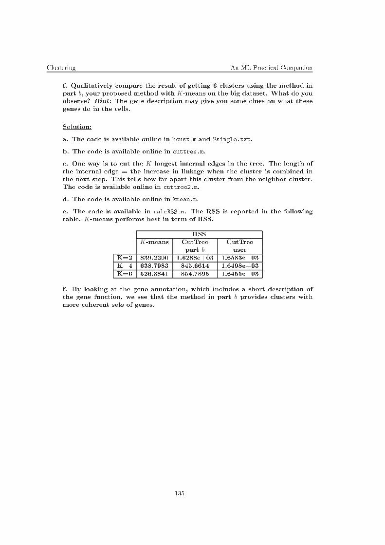
Clustering An ML Pra ti al Companion
f. Qualitatively ompare the result of getting 6 lusters using the method in
part b, your proposed method with K-means on the big dataset. What do you
observe? Hint: The gene des ription may give you some lues on what these
genes do in the ells.
Solution:
a. The ode is available online in h ust.m and 2single.txt.
b. The ode is available online in uttree.m.
. One way is to ut the K longest internal edges in the tree. The length of
the internal edge = the in rease in linkage when the luster is ombined in
the next step. This tells how far apart this luster from the neighbor luster.
The ode is available online in uttree2.m.
d. The ode is available online in kmean.m.
e. The ode is available in al RSS.m. The RSS is reported in the following
table. K-means performs best in term of RSS.
RSS
K-means CutTree CutTree
part b user
K=2 839.2200 1.6288e+03 1.6583e+03
K=4 638.7983 845.6614 1.6498e+03
K=6 526.3841 854.7895 1.6455e+03
f. By looking at the gene annotation, whi h in ludes a short des ription of
the gene fun tion, we see that the method in part b provides lusters withmore oherent sets of genes.
135

An ML Pra ti al Companion Clustering
53. (K-means: appli ation to image ompression)
• Stanford, 2012 spring, Andrew Ng, HW9
In this exer ise, you will use K-means to ompress an image by redu ing the
number of olors it ontains. To begin, download ex9Data.zip and unpa k its
ontents into your Matlab/O tave working dire tory.
Photo redit: The bird photo used in this exer ise belongs to Frank Wouters
and is used with his permission.
Image Representation
The data pa k for this exer ise ontains a 538-pixel by 538-pixel TIFF image
named bird_large.tiff. It looks like the pi ture below.
In a straightforward 24-bit olor representation of this image, ea h pixel is
represented as three 8-bit numbers (ranging from 0 to 255) that spe ify red,
green and blue intensity values. Our bird photo ontains thousands of olors,
but we'd like to redu e that number to 16. By making this redu tion, it would
be possible to represent the photo in a more e ient way by storing only the
RGB values of the 16 olors present in the image.
In this exer ise, you will use K-means to redu e the olor ount to K = 16.
That is, you will ompute 16 olors as the luster entroids and repla e ea h
pixel in the image with its nearest luster entroid olor.
136

Clustering An ML Pra ti al Companion
Be ause omputing luster entroids on a 538 × 538image would be time- onsuming on a desktop ompu-
ter, you will instead run K-means on the 128× 128 image
bird_small.tiff.
On e you have omputed the luster entroids on the small image, you will
then use the 16 olors to repla e the pixels in the large image.
K-means in Matlab/O tave
In Matlab/O tave, load the small image into your program with the following
ommand:
A = double(imread('bird_small.tiff'));
This reates a three-dimensional matrix A whose rst two indi es identify
a pixel position and whose last index represents red, green, or blue. For
example, A(50, 33, 3) gives you the blue intensity of the pixel at position y =
50, x = 33. (The y-position is given rst, but this does not matter so mu h
in our example be ause the x and y dimensions have the same size).
Your task is to ompute 16 luster entroids from this image, with ea h en-
troid being a ve tor of length three that holds a set of RGB values. Here is
the K-means algorithm as it applies to this problem:
K-means algorithm
1. For initialization, sample 16 olors randomly from the original small pi ture.
These are your K means µ1, µ2, . . . , µK .
2. Go through ea h pixel in the small image and al ulate its nearest mean.
c(i) = argminj
∥
∥
∥x(i) − µj
∥
∥
∥
2
3. Update the values of the means based on the pixels assigned to them.
µj =
∑mi 1c(i)=jx
(i)
∑mi 1c(i) = j
4. Repeat steps 2 and 3 until onvergen e. This should take between 30 and
100 iterations. You an either run the loop for a preset maximum number of
iterations, or you an de ide to terminate the loop when the lo ations of the
means are no longer hanging by a signi ant amount.
Note: In Step 3, you should update a mean only if there are pixels assigned to
it. Otherwise, you will see a divide-by-zero error. For example, it's possible
that during initialization, two of the means will be initialized to the same olor
(i.e., bla k). Depending on your implementation, all of the pixels in the photo
that are losest to that olor may get assigned to one of the means, leaving
the other mean with no assigned pixels.
Reassigning olors to the large image
137

An ML Pra ti al Companion Clustering
After K-means has onverged, load the large image into your program and
repla e ea h of its pixels with the nearest of the entroid olors you found
from the small image.
When you have re al ulated the large image, you an display and save it in
the following way:
imshow(uint8(round(large_image)))
imwrite(uint8(round(large_image)), 'bird_kmeans.tiff');
When you are nished, ompare your image to the one in the solutions.
Solution:
Here are the 16 olors appearing in the image:
© 2010-2012 Andrew Ng, Stanford University. All rights reserved.
138
Clustering An ML Pra ti al Companion
54. (K-means: how to sele t Kxxx and the initial entroids (the K-means++ algorithm);
xxx the importan e of s aling the data a ross dierent dimensions)
• CMU, 2012 fall, E. Xing, A. Singh, HW3, pr. 1
In K-means lustering, we are given points x1, . . . , xn ∈ Rdand an integer K > 1,
and our goal is to minimize the within- luster sum of squares (also known as
the K-means obje tive)
J(C,L) =n∑
i=1
||xi − Cli ||2,
where C = (C1, . . . , CK) are the luster enters (Cj ∈ Rd), and L = (l1, . . . , ln) are
the luster assignments (li ∈ 1, . . . ,K).Finding the exa t minimum of this fun tion is omputationally di ult. The
most ommon algorithm for nding an approximate solution is Lloyd's algo-
rithm, whi h takes as input the set of points and some initial luster enters
C, and pro eeds as follows:
i. Keeping C xed, nd luster assignments L to minimize J(C,L). This steponly involves nding nearest neighbors. Ties an be broken using arbitrary
(but onsistent) rules.
ii. Keeping L xed, nd C to minimize J(C,L). This is a simple step that only
involves averaging points within a luster.
iii. If any of the values in L hanged from the previous iteration (or if this was
the rst iteration), repeat from step i.
iv. Return C and L.
The initial luster enters C given as input to the algorithm are often pi ked
randomly from x1, . . . , xn. In pra ti e, we often repeat multiple runs of Lloyd's
algorithm with dierent initializations, and pi k the best resulting lustering
in terms of the K-means obje tive. You're about to see why.
a. Briey explain why Lloyd's algorithm is always guaranteed to onverge
(i.e., stop) in a nite number of steps.
b. Implement Lloyd's algorithm. Run it until onvergen e 200 times, ea h
time initializing usingK luster enters pi ked at random from the set x1, . . . , xn,with K = 5 lusters, on the 500 two dimensional data points in . . .. Plot in
a single gure the original data (in gray), and all 200 × 5 luster enters (in
bla k) given by ea h run of Lloyd's algorithm. You an play around with
the plotting options su h as point sizes so that the luster enters are learly
visible. Also ompute the minimum, mean, and standard deviation of the
within- luster sums of squares for the lusterings given by ea h of the 200
runs.
b. K-means++ is an initialization algorithm for K-means proposed by David
Arthur and Sergei Vassilvitskii in 2007:
i. Pi k the rst luster enter C1 uniformly at random from the data x1, . . . , xn.
In other words, we rst pi k an index i uniformly at random from 1, . . . , n,then set C1 = xi.
139

An ML Pra ti al Companion Clustering
ii. For j = 2, . . . ,K:
• For ea h data point, ompute its distan e Di to the nearest luster enter
pi ked in a previous iteration:
Di = minj′=1,...,j−1
||xi − Cj′ ||.
• Pi k the luster enter Cj at random from x1, . . . , xn with probabilities
proportional to D21 , . . . , D
2n. Pre isely, we pi k an index i at random from
1, . . . , n with probabilities equal to D21/(∑n
i′=1 D2i′), . . . , D
2n/(∑n
i′=1 D2i′), and
set Cj = xi.
iii. Return C as the initial luster assignments for Lloyd's algorithm.
Repli ate the gure and al ulations in part b using K-means++ as the initi-
alization algorithm, instead of pi king C uniformly at random.
735
Pi king the number of lusters K is a di ult problem. Now we will see one
of the most ommon heuristi s for hoosing K in a tion.
d. Explain how the exa t minimum of the K-means obje tive behaves on any
data set as we in rease K from 1 to n.
A ommon way to pi k K is as follows. For ea h value of K in some range
(e.g., K = 1, . . . , n, or some subset), we nd an approximate minimum of the K-
means obje tive using our favorite algorithm (e.g., multiple runs of randomly
initialized Lloyd's algorithm). Then we plot the resulting values of the K-
means obje tive against the values of K.
Often, if our data set is su h that
there exists a natural value for K,
we see a knee in this plot, i.e., a
value for K where the rate at whi h
the within- luster sum of squares
is de reasing sharply redu es. This
suggests we should use the value for
K where this knee o urs. In the
toy example in th enearby gure,
this value would be K = 6.
e. Produ e a plot similar to the one in the above gure for K = 1, . . . , 15 usingthe data set in part b, and show where the knee is. For ea h value of K, run
K-means with at least 200 initializations and pi k the best resulting lustering
(in terms of the obje tive) to ensure you get lose to the global minimum.
f. Repeat part e with the data set in . . .. Find 2 knees in the resulting plot
(you may need to plot the square root of the within- luster sum of squares
instead, in order to make the se ond knee obvious). Explain why we get 2
knees for this data set ( onsider plotting the data to see what's going on).
735
Hopefully your results make it lear how sensitive Lloyd's algorithm is to initializations, even in su h a
simple, two dimensional data set!
140

Clustering An ML Pra ti al Companion
We on lude our exploration of K-means lustering with the riti al impor-
tan e of properly s aling the dimensions of your data.
g. Load the data in . . .. Perform K-means lustering on this data with K = 2with 500 initializations. Plot the original data (in gray), and overplot the 2
luster enters (in bla k).
h. Normalize the features in this data set, i.e., rst enter the data to be
mean 0 in every dimension, then res ale ea h dimension to have unit varian e.
Repeat part g with this modied data.
As you an see, the results are radi ally dierent. You should not take this to
mean that data should always be normalized. In some problems, the relative
values of the dimensions are meaningful and should be preserved (e.g., the o-
ordinates of earthquake epi enters in a region). But in others, the dimensions
are on entirely dierent s ales (e.g., age in years v.s., in ome in thousands of
dollars). Proper pre-pro essing of data for lustering is often part of the art
of ma hine learning.
Solution:
a. The luster assignments L an take nitely many values (Kn, to be pre ise).
The luster enters C are uniquely determined by the assignments L, so afterexe uting step ii, the algorithm an be in nitely many possible states. Thus
either the algorithm stops in nitely many steps, or at least one value of
L is repeated more than on e in non- onse utive iterations. However, the
latter ase is not possible, sin e after every iteration we have J(C(t), L(t)) ≥J(C(t + 1), L(t + 1)), with equality only when L(t) = L(t + 1), whi h oin ides
with the termination ondition. (Note that this statement depends on the
assumption that the tie-breaking rule used in step i is onsistent, otherwiseinnite loops are possible.)
b. Minimum: 222.37, mean:
249.66, standard deviation: 65.64.
Plot in the nearby gure.
R ode: see le kmeans.r on the web
ourse page.
141
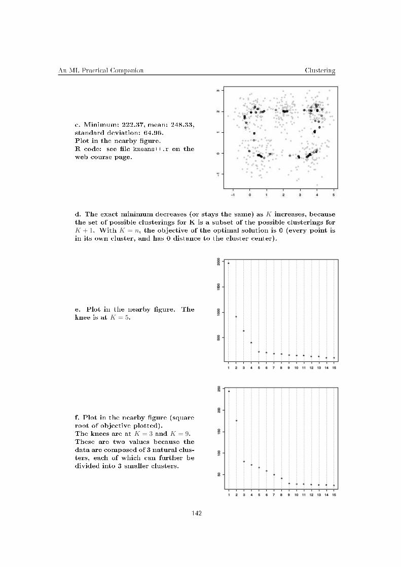
An ML Pra ti al Companion Clustering
. Minimum: 222.37, mean: 248.33,
standard deviation: 64.96.
Plot in the nearby gure.
R ode: see le kmeans++.r on the
web ourse page.
d. The exa t minimum de reases (or stays the same) as K in reases, be ause
the set of possible lusterings for K is a subset of the possible lusterings for
K + 1. With K = n, the obje tive of the optimal solution is 0 (every point is
in its own luster, and has 0 distan e to the luster enter).
e. Plot in the nearby gure. The
knee is at K = 5.
f. Plot in the nearby gure (square
root of obje tive plotted).
The knees are at K = 3 and K = 9.These are two values be ause the
data are omposed of 3 natural lus-
ters, ea h of whi h an further be
divided into 3 smaller lusters.
142
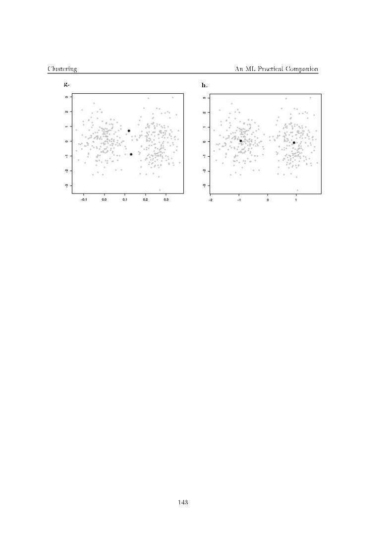
Clustering An ML Pra ti al Companion
g.
h.
143
An ML Pra ti al Companion Clustering
55. (EM/GMM: implementation in Matlab
xxx and appli ation on data from R1)
• · CMU, 2010 fall, Aarti Singh, HW4, pr. 2.3-5
a. Implement the EM/GMM algorithm using the update equations derived
in the exer ise 42, the Clustering hapter in Ciortuz et al's book).
b. Download the data set from . . .. Ea h row of this le is a training instan e
xi. Run your EM/GMM implementation on this data, using µ = [1, 2] and
θ = [.33, .67] as your initial parameters. What are the nal values of µ and θ?Plot a histogram of the data and your estimated mixture density P (X). Is themixture density an a urate model for the data?
To plot the density in Matlab, you an use:
density = (x) (< lass 1 prior> * normpdf(x, < lass 1 mean>, 1)) + ...
(< lass 2 prior> * normpdf(x, < lass 2 mean>, 1));
fplot(density, [-5, 6);
Re all from lass that EM attempts to maximize the marginal data loglikelihood
ℓ(µ, θ) =∑n
i=1 logP (X = xi;µ, θ), but that EM an get stu k in lo al optima. In this
part, we will explore the shape of the loglikelihood fun tion and determine if lo al
optima are a problem. For the remainder of the problem, we will assume that both
lasses are equally likely, i.e., θy = 12for y = 0, 1. In this ase, the data loglikelihood
ℓ only depends on the mean parameters µ.
. Create a ontour plot of the loglikelihood ℓ as a fun tion of the two mean para-
meters, µ. Vary the range of ea h µk from −1 to 4, evaluating the loglikelihood at
intervals of .25. You an reate a ontour plot in Matlab using the ontourf fun tion.
Print out your plot and in lude in with your solution.
Does the loglikelihood have multiple lo al optima? Is it possible for EM to nd a
non-globally optimal solution? Why or why not?
144

Clustering An ML Pra ti al Companion
56. (K-means and EM/GMM:
xxx omparison on data from R2)
• · CMU, 2010 spring, E. Xing, T. Mit hell, A. Singh, HW3, pr. 3
Clustering means partitioning your data into natural groups, usually be ause you
suspe t points in a luster have something in ommon. The EM algorithm and K-
means are two ommon algorithms (there are many others). This problem will have
you implement these algorithms, and explore their limitations.
The datasets for you to use are available online, along with a Matlab s ript for
loading them. [Ask me if you're having any trouble with it. You an use any
language for your implementations, but you may not use libraries whi h already
implement these algorithms (you an, however, use fan y built-in mathemati al
fun tions, like Matlab or Mathemati a provide).
a. In K-means lustering, the goal is to pi k your lusters su h that you minimize
the sum, over all points x, of |x− cx|2, where cx is the mean of the luster ontaining
x. [This should remind you of least-squares line tting. K-means lustering is NP-
hard, but in pra ti e this algoritm, also alled Lloyd's algorithm, works extremely
well.
Implement Lloyd's algorithm, and apply it to the datasets provided. Plot ea h
dataset, indi ating for ea h point whi h luster is was pla ed in. How well do you
think K-means did for ea h dataset? Explain, intuitively, what (if anything) went
badly and why.
b. A disadvantage of K-means is that the lusters annot overlap at all. The
Expe tation-Maximization algorithm deals with this by only probabilisti ally assig-
ning points to lusters.
The thing to understand about the EM algorithm is that it's a spe ial ase of MLE;
you have some data, you assume a parameterized form for the probability distri-
bution (a mixture of Gaussians is, after all, an exoti parameterized probability
distribution), and then you pi k the parameters to maximize the probability of your
data. But the usual MLE approa h, solving
∂P (X|θ)∂θ
= 0, isn't tra table, so we use
the iterative EM algorithm to nd θ. The EM algorithm is guaranteed to onverge
to a lo al optimum (I'm resisting the temptation to make you prove this :) ).
Implement the EM algorithm, and apply it to the datasets provided. Assume that
the data is a mixture of two Gaussians; you an assume equal mixing ratios. What
parameters do you get for ea h dataset? Plot ea h dataset, indi ating for ea h point
whi h luster it was pla ed in.
. Modeling dataset 2 as a mixture of gaussians is unrealisti , but the EM algorithm
still gives an answer. Is there anything shy about your answers whi h suggests
something is wrong?
We usually do the EM algorithm with mixed Gaussians, but you an use any dis-
tributions; a Gaussian and a Lapla ian, three exponentials, et . Write down the
formula for a parameterized probability density suitable for modeling ring-shaped
lusters in 2D; don't let the density be 0 anywhere. You don't need to work out the
EM al ulations for this density, but you would if this ame up in your resear h.
d. With high-dimensional data we annot perform visual he ks, and problems an
go unnoti ed if we assume ni e round, lled lusters. Des ribe in words a lustering
algorithm whi h works even for weirdly-shaped lusters with unknown mixing ration.
However, you an assume that the lusters do not overlap at all, and that you have
a LOT of training data. Dis uss the weaknesses of your algorithm. Don't work out
the details for this problem; just onvin e me that you know the basi idea and
understand its limitations.
145
An ML Pra ti al Companion Clustering
57. (EM for mixtures of multi-variate Gaussians
xxx with independent omponents (along axis):
xxx appli ation to handwritten digit re ognition)
• CMU, 2012 spring, Ziv Bar-Joseph, HW4, pr. 3.2
In this problem we will be implementing Gaussian mixture models and working
with the digits data set. The provided data set is a Matlab le onsisting of 5000
10×10 pixel hand written digits between 0 and 9. Ea h digit is a greys ale image
represented as a 100 dimensional row ve tor (the images have been down sampled
from the original 28×28 pixel images. The variable X is a 5000×100 matrix and the
ve tor Y ontains the true number for ea h image. Please submit your ode and
in lude in your write-up a opy of the plots that you generated for this problem.
a. Implement the Expe tation-Maximization (EM) algorithm for the axis aligned
Gaussian mixture model. Re all that the axis aligned Gaussian mixture model
uses the Gaussian Naive Bayes assumption that, given the lass, all features are
onditionally independent Gaussians. The spe i form of the model is given below:
Zi ∼ Categori al(p1, . . . , pK)
Xi|Zi = z ∼ N
µz1
.
.
.
µzd
,
(σz1)
2 0 . . . 0
0 (σz2)
2.
.
.
.
.
.
.
.
. 00 . . . 0 (σz
d)2
b. Run EM to t a Gaussian mixture model with 16 Gaussians on the digits data.
Plot ea h of the means using subplot(4, 4, i) to save paper.
. Evaluating lustering performan e is di ult. However, be ause we have infor-
mation about the ground truth data, we an roughly assess lustering performan e.
One possible metri is to label ea h luster with the majority label for that luster
using the ground truth data. Then, for ea h point we predi t the luster label and
measure the mean 0/1 loss. For the digits data set, report your loss for settings
k = 1, 10 and 16.
146

Clustering An ML Pra ti al Companion
58. (EM for mixtures of multi-variate Gaussians
xxx appli ation to stylus-written digit re ognition)
• MIT, 2001 fall, Tommi Jaakkola, HW4, pr. 1
147

An ML Pra ti al Companion Clustering
59. (Apli area algoritmului EM [LC: pentru GMM
xxx la lusterizare de do umente,
xxx folosind sistemul WEKA)
• Edingurgh, Chris Williams and Vi tor Lavrenko
xxx Introdu tory Applied Ma hine Learning ourse, 3 Nov. 2008
A. Des ription of the dataset
This assignment is based on the 20 Newsgroups Dataset.
736
This dataset is a ol-
le tion of approximately 20,000 newsgroup do uments, partitioned (nearly) evenly
a ross 20 dierent newsgroups, ea h orresponding to a dierent topi . Some of
the newsgroups are very losely related to ea h other (e.g. omp.sys.ibm.p .hardware,
omp.sys.ma .hardware), while others are highly unrelated (e.g. mis .forsale, so .religion. hristian).
There are three versions of the 20 Newsgroups Dataset. In this assignment we will
use the bydate Matlab version in whi h do uments are sorted by date into trai-
ning (60%) and test (40%) sets, newsgroup-identifying headers are dropped and
dupli ates are removed. This olle tion omprises roughly 61,000 dierent words,
whi h results in a bag-of-words representation with frequen y ounts. More spe i-
ally, ea h do ument is represented by a 61,000 dimensional ve tor that ontains the
ounts for ea h of the 61,000 dierent words present in the respe tive do ument.
To save you time and to make the problem manageable with limited omputational
resour es, we prepro essed the original dataset. We will use do uments from only 5
out of the 20 newsgroups, whi h results in a 5- lass problem. More spe i ally the 5
lasses orrespond to the following newsgroups 1:alt.atheism, 2: omp.sys.ibm.p .hardware,
3: omp.sys.ma .hardware, 4:re .sport.baseball and 5:re .sport.ho key. However, note here
that lasses 2-3 and 4-5 are rather losely related. Additionally, we omputed the
mutual information of ea h word with the lass attribute and sele ted the 520 words
out of 61,000 that had highest mutual information. Therefore, our dataset is a N ×520 dimensional matrix, where N is the number of do uments.
The resulting representation is mu h more ompa t and an be used dire tly to
perform our experiments in WEKA. There is, however, a potential aveat: The
prepro essed dataset has been prepared by a busy and heavily underpaid tea hing
assistant who might have been a bit areless when preparing the dataset. You
should keep this in mind and be aware of anomalies in the data when answering the
questions below.
B. Clustering
We are interested in lustering the newsgroups do uments using the EM algorithm.
The most ommon measure to evaluate the resulting lusters is the log-likelihood
of the data. We will additionally use the Classes to Clusters evaluation whi h
is straightforward to perform in WEKA, and look at the per entage of orre tly
lustered instan es. Note here that the data likelihood omputed during EM is
a probability density (NOT a probability mass fun tion) and therefore the log-
likelihood an be greater than 0. Use the train_20news_ lean_best_tdf.ar dataset
and the default seed (100) to train the lusterers.
a. First, train and evaluate an EM lusterer with 5 lusters (you need to hange the
numClusters option) using the Classes to Clusters evaluation option. Report the
log-likelihood and write down the per entage of orre tly lustered instan es (PC),
you will need it in question b. Look at the Classes to Clusters onfusion matrix.
Do the lusters orrespond to lasses? Whi h lasses are more onfused with ea h
other? Interpret your results. Keep the result buer for the lusterer, you will need
it in question c.
736
http://people. sail.mit.edu/jrennie/20Newsgroups/
148

Clustering An ML Pra ti al Companion
HINT: WEKA outputs the per entage of in orre tly lassied instan es.
b. Now, train and evaluate dierent EM lusterers using 3, 4, 6 and 7 lusters and
the Classes to Clusters evaluation option. Tabulate the PC as a fun tion of the
number of lusters, in lude the PC for 5 lusters from the previous question. What
do you noti e? Why do you think we get higher PC for 3 lusters than for 4? Keep
the result buers for all the lusterers, you will need them in question c.
. Re-evaluate the ve lusterers using the validation set val_20news_best_tdf.ar.
Tabulate the log-likelihood on the validation set as a fun tion of the number of
lusters. If the dataset was unlabeled, how many lusters would you hoose to model
it in light of your results? Is it safe to make this de ision based on experiments with
only one random seed? Why?
HINT: To re-evaluate the models, rst sele t the Supplied test set option and hoose
the appropriate dataset. Then right- li k on the model and sele t Re-evaluate model
on urrent test set.
d. Now onsider the model with 5 lusters learned using EM. After EM onverges,
ea h luster is des ribed in terms of the mean and standard deviation for ea h of
the 500 attributes omputed from the do uments assigned to the respe tive luster.
Sin e the attributes are the normalized tf-idf weights for ea h word in a do ument,
the mean ve tors learned by EM orrespond to the tf-idf weights for ea h word in
ea h luster.
For ea h of the 5 lusters, we sele ted the 20 attributes with the highest mean
values. Open the le luster_means.txt. The 20 attributes for ea h luster are displayed
olumnwise together with their orresponding mean value. By looking at the words
with the highest tf-idf weights per luster, whi h olumn ( luster) would you assign
to ea h lass (newsgroup topi ) and why? Whi h two lusters are losest to ea h
other? Imagine that we want to assign a new do ument to one of the lusters and
that the do ument ontains only the words pit hing and hit. Would this be an
easy task for the lusterer? What about a do ument that ontains only the words
drive and ma ? Write down three examples of 2-word do uments that would be
di ult test ases for the lusterer.
149

An ML Pra ti al Companion Clustering
60. (EM for GMM: appli ation on
xxx the yeast gene expression dataset)
• CMU, 2004 fall, Carlos Guestrin, HW2, pr. 3
In this problem you will implement a Gaussian mixture model algorithm and will
apply it to the problem of lustering gene expression data. Gene expression measures
the levels of messenger RNA (mRNA) in the ell. The data you will be working
with is from a model organism alled yeast, and the measurements were taken to
study the ell y le system in that organism. The ell y le system is one of the
most important biologi al systems playing a major role in development and an er.
All implementation should be done in Matlab. At the end of ea h sub-problem where
you need to implement a new fun tion we spe ify the prototype of the fun tion.
The le alphaVals.txt ontains 18 time points (every 7 minutes from 0 to 119)
measuring the log expression ratios of 745 y ling genes. Ea h row in this le
orresponds to one of the genes. The le geneNames.txt ontains the names of these
genes. For some of the genes, we are missing some of their values due to problems
with the mi roarray te hnology (the tools used to measure gene expression). These
ases are represented by values greater than 100.
a. Implement (in Matlab) an EM algorithm for learning a mixture of ve (18-
dimensional) Gaussians. It should learn means, ovarian e matri es and weights for
ea h of the Gaussian. You an assume, however, independen e between the dierent
data points [LC, orre t: features/attributes, resulting in a diagonal ovarian e
matrix. How an you deal with the missing data? Why is this orre t?
Plot the enters identied for ea h of the ve lasses. Ea h enter should be plotted
as a time-series of 18 time points.
Here is the prototype of the Matlab fun tion you need to implement:
fun tion[mu; s;w = em luster(x; k; ploton);
where
− x is input data, where ea h row is an 18-dimensional sample. Values above 100
represent missing values;
− k is the number of desired lusters;
− ploton is either 1 or 0. If 1, then before returning the fun tion plots log-likelihood
of the data after ea h EM iteration (the fun tion will have to store the log-likelihood
of the data after ea h iteration, and then plot these values as a fun tion of iteration
number at the end). If 0, the fun tion does not plot anything;
− s is a k by 18 matrix, with ea h row being diagonal elements of the orresponding
ovarian e matrix;
− w is a olumn ve tor of size k, where w(i) is a weight for i-th luster.
The fun tion outputs mu, a matrix with k rows and 18 olumns (ea h row is a enter
of a luster).
b. How many more parameters would you have had to assign if we remove the
independen e assumption above? Explain.
. Suggest and implement a method for determining the number of Gaussians (or
lasses) that are the most appropriate for this data. Please onne the set of hoi es
to values in between 2 and 7. (Hint: The method an use an empiri al evaluation
of lustering results for ea h possible number of lasses). Explain the method.
Here is the prototype of the Matlab fun tion you need to implement:
150

Clustering An ML Pra ti al Companion
fun tion[k, mu, s, w = lust(x);
where
− x is input data, where ea h row is an 18-dimensional sample. On e again values
above 100 represent missing values;
− k is the number of lasses sele ted by the fun tion;
− mu, s and w are dened as in part a.
d. Use the Gaussians determined in part c to perform hard lustering of your data
by nding, for ea h gene i the Gaussian j that maximizes the likelihood: P (i|j). Usethe fun tion printSele tedGenes.m to write the names of the genes in ea h of the
lusters to a separate le.
Here is the prototype of the matlab fun tion you need to implement:
fun tion[ = hard lust(x; k; mu; s;w);
where
− x is dened as before;
− k, mu, s, w are the output variables from the fun tion written in part c and are
therefore dened there;
− is a olumn ve tor of the same length as the number of rows in x. For ea h row,
it should indi ate the luster the orresponding gene belongs to.
The fun tion should also write out les as spe ied above. The lenames should be:
lust1, lust2, . . . , lustk.
e. Use ompSigClust.m to perform the statisti al signi an e test (everything is
already implemented here, so just use the fun tion). Hand in a printout with the
top three ategories for ea h luster (this is the output of ompSigClust.m).
Solution:
a. We have put a student ode online. The implementation is pretty lear in terms of
ea h step of the GMM iteration. The plot of the log-likelihood should be in reasing.
The plots of the enters of ea h luster should look like a sinusoid shape though
with dierent phases (starting at a dierent point in the time series).
b. The number of lusters times the number of ovarian es, whi h is
k((d− 1) + (d− 2) + . . .+ 1) =kd
2(d− 1),
where d = 18 in our ase.
. This is essentially a model sele tion question. You ould use dierent model
sele tion ways to solve it: ross validation, train-test, minimum des ription length,
BIC.
d. For ea h data point, assign the luster that has the maximum probability for this
point.
e. Just run the ode we provided on the luster les you got above.
151

An ML Pra ti al Companion EM Algorithm
8 EM Algorithm
61. (EM for Bernoulli MM, using the Naive Bayes assumption,
xxx and a penalty term;
xxx appli ation to handwritten digit re ognition)
• U. Toronto, Radford Neal,
xxx Statisti al Methods for Ma hine Learning and Data Mining ourse,
xxx 2014 spring, HW 2
In this assignment, you will lassify handwritten digits with mixture models tted
by maximum penalized likelihood using the EM algorithm. The data you will use
onsists of 800 training images and 1000 test images of handwritten digits (from
US zip odes). We derived these images from the well-known MNIST dataset, by
randomly sele ting images from the total 60000 training ases provided, redu ing
the resolution of the images from 28× 28 to 14× 14 by averaging 2× 2 blo ks of pixelvalues, and then thresholding the pixel values to get binary values. A data le with
800 lines ea h ontaining 196 pixel values (either 0 or 1) is provided on webpage
asso iated to this book. Another le ontaining the labels for these 800 digits (0 to
9) is also provided. Similarly, there is a le with 1000 test images, and another le
with the labels for these 1000 test images. You should look at the test labels only
at the very end, to see how well the methods do.
In this assignment, you should try to lassify these images of digits using a generative
model, from whi h you an derive the probabilities of the 10 possible lasses given
the observed image of a digit. You should guess that the lass for a test digit is the
one with highest probability (i.e., we will use a loss fun tion in whi h all errors are
equally bad).
The generative model we will use estimates the lass probabilities by their frequ-
en ies in the training set (whi h will be lose to, but not exa tly, uniform over the
10 digits) and estimates the probability distributions of images within ea h lass by
mixture models with K omponents, with ea h omponent modeling the 196 pixel
values as being independent. It will be onvenient to ombine all 10 of these mixture
models into a single mixture model with 10K omponents, whi h model both the
pixel values and the lass label. The probabilities for lass labels in the omponents
will be xed, however, so that K omponents give probability 1 to digit 0, K om-
ponents give probability 1 to digit 1, K omponents give probability 1 to digit 2,
et .
The model for the distribution of the label, yi, and pixel values xi,1, . . . , xi,196, for
digit i is therefore as follows:
P (yi, xi) =10K∑
k=1
πkqk,yi
196∏
j=1
θxi,j
k,j (1− θk,j)1−xi,j
The data items, (yi, xi), are assumed to be independent for dierent ases i. The
parameters of this model are the mixing proportions, π1, . . . , π10K , and the probabi-
lities of pixels being 1 for ea h omponent, θk,j for k = 1, . . . , 10K and j = 1, . . . , 196.The probabilities of lass labels for ea h omponent are xed, as
qk,y =
1 if k ∈ Ky + 1, . . . ,Ky +K0 otherwise
for k = 1, . . . , 10K and y = 0, . . . , 9.
You should write an R fun tion to try to nd the parameter values that maximize the
log-likelihood from the training data plus a penalty. (Note that with this penalty
152
EM Algorithm An ML Pra ti al Companion
higher values are better.) The EM algorithm an easily be adapted to nd maximum
penalized likelihood estimates rather than maximum likelihood estimates referring
to the general version of the algorithm, the E step remains the same, but the M
step will now maximize EQ[log P (x, z|θ) +G(θ)], where G(θ) is the penalty.
The penalty to use is designed to avoid estimates for pixel probabilities that are
zero or lose to zero, whi h ould ause problems when lassifying test ases (for
example, zero pixel probabilities ould result in a test ase having zero probability
for every possible digit that it might be). The penalty to add to the log likelihood
should be
G(θ) = α
10K∑
k=1
196∑
j=1
[log(θk,j) + log(1− θk,j)].
Here, α ontrols the magnitude of the penalty. For this assignment, you should x
α to 0.05, though in a real appli ation you would probably need to set it by some
method su h as ross-validation. The resulting formula for the update in the M step
is
θk,j =α+
∑n
i=1 ri,kxi,j
2α+∑n
i=1 ri,k
where ri,k is the probability that ase i ame from omponent k, estimated in the E
step. You should write a derivation of this formula from the general form of the EM
algorithm presented in the le ture slides (modied as above to in lude a penalty
term).
Your fun tion implementing the EM algorithm should take as arguments the ima-
ges in the training set, the labels for these training ases, the number of mixture
omponents for ea h digit lass (K), the penalty magnitude (α), and the number of
iterations of EM to do. It should return a list with the parameter estimates (π and
θ) and responsibilities (r). You will need to start with some initial values for the
responsibilities (and then start with an M step). The responsibility of omponent
k for item i should be zero if omponent k has qk,yi = 0. Otherwise, you should
randomly set ri,k from the uniform distribution between 1 and 2 and then res ale
these values so that for ea h i, the sum over k of ri,k is one.
After ea h iteration, your EM fun tion should print the value of the log-likelihood
and the value of the log likelihood plus the penalty fun tion. The latter should never
go down if it does, you have a bug in your EM fun tion. You should use enough
iterations that these values have almost stabilized by the last iteration.
You will also need to write an R fun tion that takes the tted parameter values
from running EM and uses them to predi t the lass of a test image. This fun tion
should use Bayes' Rule to nd the probability that the image ame from ea h of the
10K mixture omponents, and then add up the probabilities for the K omponents
asso iated with ea h digit, to obtain the probabilities of the image being of ea h
digit from 0 to 9. It should return these probabilities, whi h an then be used to
guess what the digit is, by nding the digit with the highest probability.
You should rst run your program EM and predi tion fun tions for K = 1, whi hshould produ e the same results as the naive Bayes method would. (Note that EM
should onverge immediately with K = 1.) You should then do ten runs with K = 5using dierent random number seeds, and see what the predi tive a ura y is for
ea h run. Finally, for ea h test ase, you should average the lass probabilities ob-
tained from ea h of the ten runs, and then use these averaged probabilities to lassify
the test ases. You should ompare the a ura y of these ensemble predi tions
with the a ura y obtained using the individual runs that were averaged.
You should hand in your derivation of the update formula for θ above, a listing of
the R fun tions you wrote for tting by EM and predi ting digit labels, the R s ripts
you used to apply these fun tions to the data provided, the output of these s ripts,
in luding the lassi ation error rates on the test set you obtained (with K = 1,
153

An ML Pra ti al Companion EM Algorithm
with K = 5 for ea h of ten initializations, and with the ensemble of ten ts with
K = 5), and a dis ussion of the results. Your dis ussion should onsider how naive
Bayes (K = 1) ompares to using a mixture (with K = 5), and how the ensemble
predi tions ompare with predi ting using a single run of EM, or using the best run
of EM a ording to the log likelihood (with or without the penalty).
Solution:
With K = 1, whi h is equivalent to a naive Bayes model, the lassi ation error rate
on test ases was 0.190.
With K = 5, 80 iterations of EM seemed su ient for all ten random initializations.
The resulting models had the following error rates on the test ases:
0.157 0.151 0.158 0.156 0.166 0.162 0.163 0.159 0.158 0.153
These are all better than the naive Bayes result, showing that using more than one
mixture omponent for ea h digit is bene ial.
I used the show_digit fun tion to display the theta parameters of the 50 mixture
omponents as pi tures (for the run started with the last random seed). It is lear
that the ve omponents for ea h digit have generally aptured reasonable variations
in writing style, ex ept perhaps for a few with small mixing proportion (given as
the number above the plot), su h as the se ond 1 from the top.
154

EM Algorithm An ML Pra ti al Companion
Using the ensemble predi tions (averaging probabilities of digits over the ten runs
above), the lassi ation error rate on test ases was 0.139. This is substantially
better than the error rate from every one of the individual runs, showing the benets
of using an ensemble when there is substantial random variation in the results.
Note that the individual run with highest log likelihood (and also highest log likeli-
hood + penalty) was the sixth run, whose error rate of 0.162 was a tually the third
worst. So at least in this example, pi king a single run based on log likelihood would
ertainly not do better than using the ensemble.
155

An ML Pra ti al Companion EM Algorithm
62. (EM for a mixture of two exponential distributions)
• · U. Toronto, Radford Neal,
xxx Statisti al Computation ourse,
xxx 2000 fall, HW 4
Suppose that the time from when a ma hine is manufa tured to when it fails is
is exponentially distributed (a ommon, though simplisti , assumption). However,
suppose that some ma hines have a manufa turing defe t that auses them to be
more likely to fail early than ma hines that don't have the defe t.
Let the probability that a ma hine has the defe t be p, the mean time to failure for
ma hines without the defe t be g, and the mean time to failure for ma hines with
the defe t be d. The probability density for the time to failure will then be the
following mixture density:
p ·1
µd
· exp
(
−x
µd
)
+ (1− p) ·1
µg
exp
(
−x
µg
)
Suppose that you have a number of independent observations of times to failure
for ma hines, and that you wish to nd maximum likelihood estimates for p, µg,
and µd. Write a program to nd these estimates using the EM algorithm, with
the unobserved variables being the indi ators of whether or not ea h ma hine is
defe tive. Note that the model is not identiable swapping µd and µg while
repla ing p with 1− p has no ee t on the density. This isn't really a problem; you
an just interpret whi hever mean is smaller as the mean for the defe tive ma hines.
You may write your program so that it simply runs for however many iterations you
spe ify (i.e., you don't have to ome up with a onvergen e test). However, your
program should have the option of printing the parameter estimates and the log
likelihood at ea h iteration, so that you an manually see whether it has onverged.
(This will also help debugging.)
You should test your program on two data sets (ass4a.data and ass4b), ea h with 1000
observations, whi h are on the web page asso iated to this book. You an read this
data with a ommand like
> x <- s an("ass4a.data")
For both data sets, run your algorithm for as long as you need to to be sure that
you have obtained lose to the orre t maximum likelihood estimates. To be sure,
we re ommend that you run it for hundreds of iterations or more (this shouldn't
take long in R). Dis uss how rapidly the algorithm onverges on the two data sets.
You may nd it useful to generate your own data sets, for whi h you know the true
parameters values, in order to debug your program. You ould start with data sets
where µg and µd are very dierent.
You should hand in your derivation of the formulas neeed for the EM algorithm,
your program, the output of your tests, and your dis ussion of the results.
156