Submission for the Special Issue of Simulation: Software Tools,

Techniques and Architectures for Computer Simulation

PowerDEVS. A Tool for Hybrid System Modeling

and Real Time Simulation.

Federico Bergero†, Ernesto Kofman†

†Laboratorio de Sistemas Dinamicos. FCEIA - UNR. CIFASIS–CONICET.Riobamba 245 bis - (2000) Rosario, Argentina

bergero@cifasis-conicet.gov.ar kofman@fceia.unr.edu.ar

Abstract

This paper introduces a general purpose software tool for DEVS mod-eling and simulation oriented to the simulation of hybrid systems. Theenvironment –called PowerDEVS - allows defining atomic DEVS modelsin C++ language that can be then graphically coupled in hierarchicalblock diagrams to create more complex systems. The environment au-tomatically translates the graphically coupled models into a C++ codewhich executes the simulation.

A remarkable feature of PowerDEVS is the possibility of perform-ing simulations under a real–time operating system (RTAI) synchronizingwith a real time clock, which permits the design and automatic imple-mentation of synchronous and asynchronous digital controllers. Com-bined with its continuous system simulation library, PowerDEVS is alsoan efficient tool for real time simulation of physical systems.

Another feature is the interconnection between PowerDEVS and thenumerical package Scilab. PowerDEVS simulations can make use of Scilabworkspace variables and functions, and the results can be sent back toScilab for further processing and data analysis.

Besides describing the main features of the software tool, the articlealso illustrates its use with some examples which show its simplicity andefficiency.

Keywords: DEVS, Hybrid Systems, Real Time Simulation, SimulationSoftware

1 INTRODUCTION

DEVS [32] is the most general formalism for discrete event system modeling.It allows representing any system provided that it performs a finite number ofchanges in finite intervals of time. Thus, not only Petri–Nets, State–charts,Event–Graphs and other discrete event languages but also all discrete timesystems can be seen as particular cases of DEVS [30, 23].

1

Taking into account that ordinary differential equations can be approximatedby discrete time systems –using numerical integration methods– and that thesesystems are particular cases of DEVS, it results that DEVS can also approximatecontinuous systems. Moreover, there are numerical methods –like the QuantizedState System (QSS) family [4]– which produce simulation models that cannotbe represented in discrete time but only as DEVS models.

Thus, simulation tools based on DEVS are potentially more general thantools for different discrete formalisms, including the popular continuous timeones as Simulink [14] (Matlab), Scicos [3] (Scilab), etc.

Among the existing DEVS simulation tools we should mention DEVS–Java[31], DEVSim++ [13], DEVS–C++ [6], CD++ [25] and JDEVS [7].

These software tools offer different features which include graphical inter-faces and advanced simulation features for general purpose DEVS models andfor some specific domains. However, they were developed before the mentioneddiscrete event methods for numerical integration of ordinary differential equa-tions (ODEs).

These methods produce DEVS models with some very particular features onone hand. In fact, they are usually composed of several atomic DEVS modelswhich belong to two basic classes: quantized integrators and static functions.The different quantized integrators differ from each other in only two parame-ters: the quantum and the initial state value. Similarly, different static functionsonly differ in some parameters as the gain, number of inputs, the calculated ex-pression, etc.

On the other hand, these new numerical methods have many potential usersoutside the DEVS–working community. In strongly discontinuous systems theQSS methods offer solutions which are sensibly better than existing numericalalgorithms [18] and they are starting to be used by continuous system simulationpeople. Unfortunately, most researchers and users of numerical ODE integrationmethods do not know about DEVS and they would appreciate to use the DEVS–based methods without learning DEVS. Moreover, they would be happier if thesoftware they have to use looks similar to the software they use for conventionalnumerical methods (Simulink, Dymola, Scicos, etc.).

Taking into account these remarks, a DEVS simulation environment with li-brary handling capabilities and a block–oriented graphical interface like Simulinkwhere parameters can be changed without modifying the blocks and where theatomic DEVS definitions are hidden for non–DEVS–users appears as an appro-priate solution for hybrid system simulation.

These ideas motivated the development of a general purpose DEVS simula-tion software oriented to hybrid system simulation. Here, we call hybrid systemany system involving simultaneous continuous (represented by ODEs) and dis-crete (represented by DEVS) dynamics.

This software package, called PowerDEVS was conceived to be used byDEVS expert programmers as well as by end users who only want to connectpredefined blocks and simulate. The tool, initially developed as a Diploma Work[22] in our University, was then re-written and is currently maintained by theLaboratory for System Dynamics and Signal Processing.

PowerDEVS is composed of various independent programs:

• The Model Editor, which contains the graphical interface allowing thehierarchical block-diagram construction, library managing, parameter se-

2

lection and other high level definitions as well as providing the linkingwith the other programs.

• The Atomic Editor, which permits editing DEVS atomic models of el-ementary blocks by defining transition functions, output function, timeadvance, etc.

• The Preprocessor, which translates the model editor files into structurefiles which contain the coupling structure and the information to buildup the simulation code, links the code of the different atomic modelsaccording to the corresponding structure file and compiles it to produce astand alone executable file which simulates the system.

• The Simulation Interface, which runs the stand alone executable and per-mits to vary simulation parameters such as final time, number of simu-lations to perform, and the simulation mode (normal simulation, timedsimulation, step-by-step simulation,etc).

• A running instance of Scilab, which acts as a workspace, where simulationparameters can be read, and results can be exported to. This instance isa modification of Scilab 4.1.2 to support this type of operations.

All these applications were programmed in C++ with the graphical librariesQT, with the exception of the Model Editor that was programmed in Visual Ba-sic. We provide compiled versions of these applications for Linux and Windows,and all the source code is available for download too.

PowerDEVS also runs under a real time operating system (RTAI[19]) syn-chronizing the events with a real–time clock with the capability of capturinginterrupts at the atomic level. To this purpose, the DEVS simulation scheme of[32] was partially inverted so that simulators of atomic models can send messagesto their parents informing about the next event time. In this way, PowerDEVSallows the direct implementation of asynchronous DEVS–based Quantized StateControllers [17] on a PC. Besides the Linux and Windows distributions, we de-veloped a modified Kubuntu distribution that includes the RTAI kernel andPowerDEVS.

The paper is organized as follows: Section 2 introduces the main conceptsused in the rest of the article. Then, Section 3 describes the main featuresof PowerDEVS and Section 4 analyzes its real time characteristics. Finally,Section 5 illustrates the usage of PowerDEVS in two examples (including a realtime control application) and Section 6 concludes the article.

2 BACKGROUND

2.1 DEVS

DEVS stands for Discrete EVent System specification, a formalism introducedfirst by Bernard Zeigler [29].

A DEVS model processes an input event trajectory and –according to thattrajectory and its own initial conditions– it provokes an output event trajectory.

An atomic DEVS model is defined by the following structure:

M = (X, Y, S, δint, δext, λ, ta)

3

where:

• X is the set of input event values, i.e., the set of all possible values thatan input event can adopt.

• Y is the set of output event values.

• S is the set of state values.

• δint, δext, λ and ta are functions which define the system dynamics.

Each possible state s (s ∈ S) has an associated Time Advance computed bythe Time Advance Function ta(s) (ta(s) : S → ℜ

+

0 ). The Time Advance is anon-negative real number saying how long the system remains in a given statein absence of input events.

Thus, if the state adopts the value s1 at time t1, after ta(s1) units of time(i.e. at time ta(s1) + t1) the system performs an internal transition going toa new state s2. The new state is calculated as s2 = δint(s1). Function δint

(δint : S → S) is called Internal Transition Function.When the state goes from s1 to s2 an output event is produced with value

y1 = λ(s1). Function λ (λ : S → Y ) is called Output Function. In that way, thefunctions ta, δint and λ define the autonomous behavior of a DEVS model.

When an input event arrives the state changes instantaneously. The newstate value depends not only on the input event value but also on the previousstate value and the elapsed time since the last transition. If the system arrivedto the state s2 at time t2 and then an input event arrives at time t2+e with valuex1, the new state is calculated as s3 = δext(s2, e, x1) (note that ta(s2) > e). Inthis case, we say that the system performs an external transition. Function δext

(δext : S × ℜ+

0 × X → S) is called External Transition Function. No outputevent is produced during an external transition.

The formalism presented is also called Classic DEVS to distinguish it fromParallel DEVS [32], which consists in an extension of the previous one conceivedto improve the treatment of simultaneous events.

Atomic DEVS models can be coupled. DEVS theory guarantees that thecoupling of atomic DEVS models defines new DEVS models (i.e. DEVS isclosed under coupling) and then complex systems can be represented by DEVSin a hierarchical way [32].

Coupling in DEVS is usually represented through the use of input and outputports. With these ports, the coupling of DEVS models becomes a simple block–diagram construction. Figure 1 shows a coupled DEVS model N which is theresult of coupling the models Ma and Mb.

According to the closure property, the model N can be used itself as anatomic DEVS and it can be coupled with other atomic or coupled models.

2.2 SIMULATING A DEVS MODEL

One of the most important features of DEVS is that very complex models canbe simulated in a very easy and efficient way.

The basic idea for the simulation of a coupled DEVS model can be describedby the following steps:

4

Ma

Mb

N

Figure 1: Coupled DEVS model

atomic1 atomic2atomic3

coupled1

coupled2

simulator1 simulator2

simulator3coordinator1

coordinator2

root − coordinator

Figure 2: Hierarchical model and simulation scheme

1. Look for the atomic model that, according to its time advance and elapsedtime, is the next to perform an internal transition. Call it d∗ and let tn

be the time of the mentioned transition.

2. Advance the simulation time t to t = tn and execute the internal transitionfunction of d∗.

3. Propagate the output event produced by d∗ to all the atomic models con-nected to it executing the corresponding external transition functions.Then, go back to step 1.

One of the simplest ways to implement these steps is writing a program with ahierarchical structure equivalent to the hierarchical structure of the model to besimulated. This is the method developed in [32] where a routine called DEVS-simulator is associated to each atomic DEVS model and a different routinecalled DEVS-coordinator is related to each coupled DEVS model. At the top ofthe hierarchy there is a routine called DEVS-root-coordinator which managesthe global simulation time.

Figure 2 illustrates this idea over a coupled DEVS model.The simulators and coordinators of consecutive layers communicate with

each other with messages. The coordinators send messages to their children sothey execute the transition functions. When a simulator executes a transition,it calculates its next state and –when the transition is internal– it sends the

5

output value to its parent coordinator. In all the cases, the simulator state willcoincide with its associated atomic DEVS model state.

When a coordinator executes a transition, it sends messages to some of itschildren so they execute their corresponding transition functions. When anoutput event produced by one of its children has to be propagated outside thecoupled model, the coordinator sends a message to its own parent coordinatorcarrying the output value.

Each simulator or coordinator has a local variable tn which indicates the timewhen its next internal transition will occur. In the simulators, that variable iscalculated using the time advance function of the corresponding atomic model.In the coordinators, it is calculated as the minimum tn of their children. Thus,the tn of the coordinator at the top is the time at which the next event of theentire system will occur. Then, the root coordinator only looks at this time,advances the global time t to this value and then it sends a message to its childso it performs the next transition, and then it repeats this cycle until the endof the simulation.

2.3 DEVS AND HYBRID SYSTEMS SIMULATION

Hybrid systems combine discrete and continuous dynamics. While discrete sub-systems have a straightforward representation in DEVS, continuous submodelsrequire some type of discretization.

Although DEVS can easily represent the discrete time approximations ofcontinuous systems given by conventional numerical integration methods suchas Euler, Runge Kutta, etc., it can also represent the approximations resultingfrom state quantization. Quantization based integration methods are noticeablyefficient to simulate hybrid systems due to their ability to handle discontinuities.

2.3.1 QUANTIZATION BASED INTEGRATION

Continuous time systems can be written as set of ordinary differential equations(ODEs):

x(t) = f(x(t),u(t)) (1)

where x ∈ ℜn is the state vector and u ∈ ℜm is a vector of known inputfunctions.

The simulation system (1) requires using numerical integration methods.While conventional integration algorithms are based on time discretization, anew family of numerical methods was developed based on state quantization [4].The new algorithms, called Quantized State System methods (QSS methods),can approximate ODEs like that of Eq.(1) by DEVS models.

Formally, the first order accurate QSS method approximates Eq.(1) by

x(t) = f(q(t),v(t)) (2)

where each pair of variables qj and xj are related by a hysteretic quantizationfunction.

The presence of a hysteretic quantization function relating qj(t) and xj(t)implies that qj(t) follows a piecewise constant trajectory that only changes whenthe difference with xj(t) becomes equal to a parameter ∆qj called quantum.

6

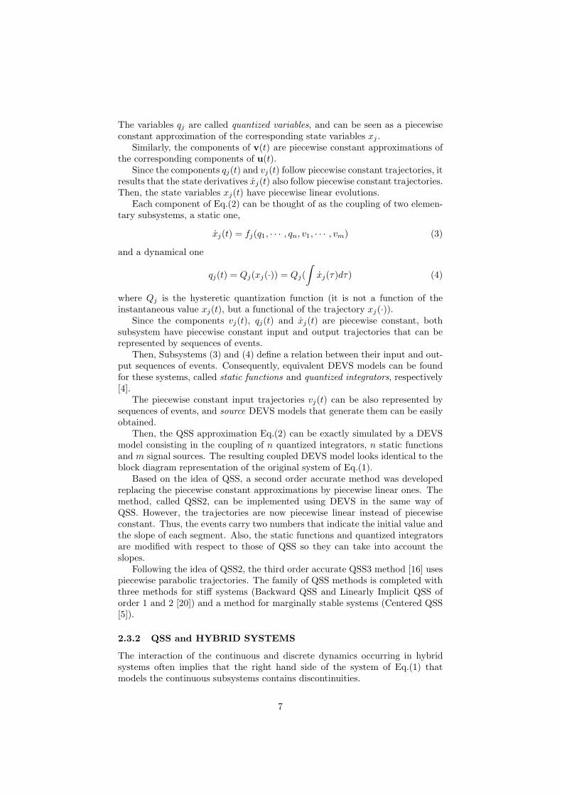
The variables qj are called quantized variables, and can be seen as a piecewiseconstant approximation of the corresponding state variables xj .

Similarly, the components of v(t) are piecewise constant approximations ofthe corresponding components of u(t).

Since the components qj(t) and vj(t) follow piecewise constant trajectories, itresults that the state derivatives xj(t) also follow piecewise constant trajectories.Then, the state variables xj(t) have piecewise linear evolutions.

Each component of Eq.(2) can be thought of as the coupling of two elemen-tary subsystems, a static one,

xj(t) = fj(q1, · · · , qn, v1, · · · , vm) (3)

and a dynamical one

qj(t) = Qj(xj(·)) = Qj(

∫

xj(τ)dτ) (4)

where Qj is the hysteretic quantization function (it is not a function of theinstantaneous value xj(t), but a functional of the trajectory xj(·)).

Since the components vj(t), qj(t) and xj(t) are piecewise constant, bothsubsystem have piecewise constant input and output trajectories that can berepresented by sequences of events.

Then, Subsystems (3) and (4) define a relation between their input and out-put sequences of events. Consequently, equivalent DEVS models can be foundfor these systems, called static functions and quantized integrators, respectively[4].

The piecewise constant input trajectories vj(t) can be also represented bysequences of events, and source DEVS models that generate them can be easilyobtained.

Then, the QSS approximation Eq.(2) can be exactly simulated by a DEVSmodel consisting in the coupling of n quantized integrators, n static functionsand m signal sources. The resulting coupled DEVS model looks identical to theblock diagram representation of the original system of Eq.(1).

Based on the idea of QSS, a second order accurate method was developedreplacing the piecewise constant approximations by piecewise linear ones. Themethod, called QSS2, can be implemented using DEVS in the same way ofQSS. However, the trajectories are now piecewise linear instead of piecewiseconstant. Thus, the events carry two numbers that indicate the initial value andthe slope of each segment. Also, the static functions and quantized integratorsare modified with respect to those of QSS so they can take into account theslopes.

Following the idea of QSS2, the third order accurate QSS3 method [16] usespiecewise parabolic trajectories. The family of QSS methods is completed withthree methods for stiff systems (Backward QSS and Linearly Implicit QSS oforder 1 and 2 [20]) and a method for marginally stable systems (Centered QSS[5]).

2.3.2 QSS and HYBRID SYSTEMS

The interaction of the continuous and discrete dynamics occurring in hybridsystems often implies that the right hand side of the system of Eq.(1) thatmodels the continuous subsystems contains discontinuities.

7

If a numerical integration method performs an integration step that crossesthrough a discontinuity, the result will have an unacceptable error.

Conventional numerical methods solve this problem by finding the instantof time at which the discontinuity occurs (this is usually called zero crossing).Then, they advance the simulation up to that point, and they restart the inte-gration from the new condition (after the event).

Although this idea works fine, it adds some computational cost: zero crossingdetection implies performing some iterations and the simulation restart can bealso quite expensive. Due to the presence of unbounded iterations, this solutionis usually unacceptable in the context of real time simulation [4].

Besides these difficulties, the simulation of a hybrid system requires also therepresentation and simulation of the remaining discrete subsystems, which inturn calls for the use of a common scheduling algorithm.

The usage of QSS methods on a DEVS simulation engine solves all thementioned problems. On one hand, DEVS provides the unified framework torepresent the discrete and the continuous (quantized) dynamics and to couplethem on a single model.

Also, according to the order of the QSS method used, the trajectories arepiecewise linear, parabolic or cubic. Thus, the zero crossing detection can beanalytically solved, without performing iterations at all.

Although the event associated to a discontinuity must occur at the righttime, the methods do not need to restart after that. After all, discontinuities inQSS occur all the time, as the trajectories of qj(t) are discontinuous. Thus, forthe QSS approximations, a discontinuity has the same effect of a normal step.

Moreover, when a component fj of the system (1) contains a discontinuity,the DEVS static function computing xj(t) will be in charge of detecting thediscontinuity and provoking the right event trajectory for the state derivative.In other words, discontinuities are detected and handled locally, without anyadditional computational cost for the rest of the simulation.

These advantages result in a noticeable simulation speedup with respect toconventional numerical algorithms. In models with rapidly occurring disconti-nuities such as power electronic systems, the high order QSS2 and QSS3 andLIQSS2 can perform simulations up to 20 times faster than all existing conven-tional methods [18].

2.4 SIMILAR TOOLS

There is a great variety of tools in the field of DEVS simulation. Some are plainDEVS simulators, without real time support, and others are general continuoussystem simulation tools. Here we describe a few of these tools.

• ADEVS [21] is a C++ library to simulate DEVS based models. UnlikePowerDEVS it is based on two DEVS formalism extensions, called ParallelDEVS and Dynamic DEVS which treat simultaneous events in a differentway (confluent transition). ADEVS is a library, but it does not have a GUIfor model coupling and the model has to be described alphanumerically.

• CD++[24] is a DEVS simulation tool developed by Gabriel Wainer’sgroup. It is based on another DEVS extension, called Cell-DEVS, whichmerges DEVS and cellular automata. It has support for real time simula-tion.

8

• DEVSJava[32, 11] is a DEVS simulation tool developed by Bernard Zeiglerand Hessam Sarjoughian. It has interesting features such as changingthe model structure at run time (or simulation time). Also, it offers ahierarchical view of the model structure. It has support for real timesimulation in a best shot way, because it is written in Java and runs undernon-real-time Operating Systems.

• Matlab Real Time Workshop[12] is a toolbox of Simulink. Simulink is atool for modeling and simulation of continuous systems. It has a GUI inwhich models can be described in a Block Diagram fashion. It supportsgenerating C++ code for running the simulation under a variety of RTOS.The Real Time Workshop (being a part of Matlab) is a proprietary soft-ware of The MathWorks and its use and distribution is restricted by itslicense.

3 POWERDEVS

In this section we describe the main components and features of the softwaredeveloped.

3.1 POWERDEVS COMPONENTS

As we mentioned, PowerDEVS is composed of various independent programs:the model editor, the atomic editor, the preprocessor and the simulation interfaceand a workspace corresponding to a Scilab instance.

In this section we describe each of this tools and how they interact whicheach other.

3.1.1 THE MODEL EDITOR

The Model Editor is –from a user point of view– the main program of Pow-erDEVS as it provides the graphical interface and the link with the rest of theapplications.

Besides building and managing models and libraries, it permits launching asimulation (by invoking the Preprocessor) and editing elementary blocks up tothe atomic model definitions (by invoking the Atomic Editor).

The Model Editor main window (Fig. 3) allows the user to create and openmodels and libraries. It also permits exploring the libraries and dragging blocksfrom the libraries to the models.

Figure 3: Model Editor main window.

9

There are also some advanced features which can be managed from the mainwindow like setting which are the active libraries (i.e. which libraries are shownwhen exploring), and configuring the tool bars and menu to invoke new externalapplications.

Models and libraries can be edited in a model window with the open andnew model commands. Figure 4 shows a model window with a model composedby five sub–models.

Figure 4: Model Window.

The Model Windows provide all the typical graphical edition facilities sothat blocks can be copied, resized, rotated, etc. while the connections can bedirectly drawn between different ports.

From the edit menu (or with the right button) it is possible to edit thefeatures of each block, no matter if it corresponds to a coupled or an atomicmodel.

The Block Edition Window (Fig. 5) allows to configure the graphic appear-ance of the block, to choose the block parameters and –in the case of atomicmodels– to select the file which contains the associated code with the DEVSmodel definitions.

The block parameters are defined and selected in the block edition windows.After being defined, their values can be changed by double–clicking on the block(Fig. 6). Thus, when we take predefined blocks from the libraries, we can changethe parameter values without editing them. As we shall see in Section 3.1.3,the values of these parameters are passed to the corresponding DEVS atomicor coupled models.

Coupled models do not have an associated code, but they have some extrafeatures which can be modified from the block edition window and the editmenu (the internal priorities and the order of the input and output ports, forinstance).

10

Figure 5: Block Edition Window.

Figure 6: Changing parameter values.

3.1.2 THE ATOMIC EDITOR

The Atomic Editor facilitates the edition of the C++ code corresponding toeach atomic DEVS model.

It can be invoked from the Block Edition Window to edit an existing codeor to create a new one. It can be also run directly from the OS since it is astand alone application. The Atomic Editor main window is shown in Figure 7.

Using the atomic editor, the user only has to define the variables which formthe state and the output of the DEVS model and the variables which representthe parameters of the system. After that, the C++ code of the time advance,transition and output functions must be placed in the corresponding windows.There are two additional windows (init and exit) where the user can also add apiece of code that is executed before the simulation starts (to set initial statesand parameters, for instance) and a piece of code that is executed at the end ofthe simulation (to close some open files, for instance). When the model is saved,the code is automatically completed and stored in the corresponding .cpp and

11

Figure 7: Atomic Editor main window.

.h files.Besides facilitating the programming, the Atomic Editor was designed to give

the user the possibility of writing a code which is very similar to the DEVS modeldefinition. All the rest of the job –related to simulation and implementationissues– is automatically performed by the program.

Let us illustrate this fact with a simple DEVS model. Consider for instancea system which calculates a static function f(u0, u1) = u0 − u1 with u0 and u1

being real-valued piecewise constant trajectories. If we represent those trajec-tories by sequences of events –as it is done in QSS–methods– we can build thefollowing atomic DEVS model:

M = (X, Y, S, δint, δext, λ, ta), where

S = ℜ2×ℜ

+

δint(s) = δint(u0, u1, σ) = (u0, u1,∞)

δext(s, e, x) = δext(u0, u1, σ, e, xv, p) = s

λ(s) = λ(u0, u1, σ) = (u0 − u1, 0)

ta(s) = ta(u0, u1, σ) = σ

with

s =

(xv, u1, 0) if p = 0(u0, xv, 0) otherwise

We use integer numbers from 0 to n − 1 to denote the input and output ports(because PowerDEVS does so).

This DEVS model translated into PowerDEVS has the following code (atthe Atomic Editor Fig. 7):

ATOMIC MODEL STATIC1

State Variables and Parameters:

12

float u[2],sigma; //statesfloat y; //outputfloat inf ; //parameter

Init Function:

inf = 1e10;u[0] = 0;u[1] = 0;sigma = inf ;y = 0;

Time Advance Function:

return sigma;

Internal Transition Function:

sigma=inf ;

External Transition Function:

float xv;xv=*(float*)(x.value);u[x.port] = xv;sigma = 0;

Output Function:

y = u[0] − u[1];return Event(&y,0);

It is clear that the translation from the atomic DEVS into the PowerDEVS codeis almost straightforward.

With that code, the Atomic Editor automatically produces the .cpp and .hfiles which are then used by the Preprocessor to generate the simulation of thewhole system.

3.1.3 THE PREPROCESSOR

The Preprocessor takes a .pdm (or .pds) file produced by the model editor andproduces the simulation program.

It basically translates the .pdm file into a header .h file (called model.h)which binds the simulators and coordinators according to the coupling structurepassing also the block parameters.

The preprocessor also produces a makefile (Makefile.include) which is theninvoked to compile and generate the program which implements the simulation(that program is called model).

As we mentioned before, the Preprocessor can be invoked in a transparentway using the Quick Simulation command. Anyway, it can be also called fromthe command line (it is also a stand alone application).

3.1.4 THE SIMULATION INTERFACE

The generated program model, when executed, simulates the associated DEVSmodel.

PowerDEVS provides a graphical interface for running the simulation (Fig. 8).The interface also allows to change some parameters to set up the experi-

ment:

• Final Time: tells for how long to simulate the model.

13

Figure 8: Simulation Interface

• Simulations to run: multiple simulation runs can be executed at once. Thiscan be useful when statistics from simulation results are to be calculated.

• Illegitimate check break: PowerDEVS stops the simulation if the timedoes not advance after a selected number of steps. This avoids hang-upsin illegitimate models.

• Simulate step-by-step: the simulation can be advanced performing onestep (or many) at the time, and results can be analyzed in between.

• Synchronize time: The simulation can be run synchronized with the realclock (with the precision of the underlying OS).

Also, the model program can be invoked from the command line, and exe-cuted in an interactive shell. All the simulation parameters can be changed inthe same way they are changed from the graphical interface.

3.2 INTERNAL IMPLEMENTATION

Having described the main functional aspects of PowerDEVS, we shall nowexplain the way in which the simulation algorithm described in Section 2.2 isimplemented inside the program that executes the simulation.

As PowerDEVS performs an object oriented simulation, we shall start de-scribing the internal class structure.

Atomic models with the same associated code belong to a particular class(defined by that code). For instance, the Integrator atomic models in the modelof Fig. 4 belong to the Integrator class, defined in the files integrator.h andintegrator.cpp which contain the code associated to that atomic model.

14

When the code of an atomic model is written using the Atomic Editor, thecode related to the class definition is automatically generated.

All the atomic classes are derived from the simulator class. The simulatorclass is an abstract class which acts as an interface to deal with different atomicmodel implementations. The variables representing the state of the model andthe functions that operate on it (time advance, transition and output functions)are member variables and methods.

The external transition and output functions of the simulator class receiveand return respectively objects belonging to the Event class. Events have thefollowing properties:

• Event.port: is an integer number indicating the input or output port wherethe event is received or sent.

• Event.value: is a pointer to void. That way, the values carried by theevents can belong to arbitrary types.

• Event.realTimeMode: is an integer that can take the following values: 0(indicating that the event is not synchronized with the real time), 1 (withnormal synchronization) and 2 (with precise synchronization). When anevent has its mode set to 1 or 2 (the difference between them will beexplained in Section 4.2.1), the simulation engine waits until the physicaltime reaches the simulation time to propagate it.

To provide the capability of initializing and stopping devices that interactwith the hardware, the simulator class has two extra methods which are notincluded in the definition of [32]. As we already mentioned, for real–time sim-ulation purposes PowerDEVS also inverts the time managing features. Thus,when an atomic model receives an interrupt request from an external device, itinforms the change in its time to next event (tn) to its parent.

The hierarchical coupling structure is implemented by the coupling class.This class is similar to the coordinator in Fig. 2. Each object of this class isassociated to a coupled DEVS model and it contains a list of references to thecorresponding connections, atomic and coupled models.

The difference with the coordinator is that, following the simulator classbehavior, the coupling objects are able to receive the messages coming fromtheir children notifying changes in their time to next event. Similarly, thecoupling objects have also the possibility of informing their own parent aboutchanges in their tn. Coherently with the closure property, the coupling class isderived from the simulator class.

The coupling and simulator objects also contain objects belonging to theclasses connection and event (the first one is only in the coupling class). Theconnection class is formed by four integer numbers representing two pairs ofmodels and ports. The event objects are formed by a pointer to void and aninteger (identifying the input or output port). Thus PowerDEVS models canproduce output events which belong to different types.

Having defined the model structure in terms of components and function-ality, we shall now describe the framework developed to actually execute thesimulation.

The root–simulator class is in charge of running the simulation. Basically,this class manages the simulation advance interacting with the object represent-

15

ing the coupling at the top of the structure. Thus, the root–simulator plays therole of the root–coordinator in Fig. 2.

Before following the description we should mention that the behavior of thetop coupling object has a small difference with the others. In terms of thesimulation execution, there is no coupling above to notify the timing changesbut these changes should be notified directly to the root–simulator. Thus, a newclass denominated root–coupling has been introduced. This class, derived fromthe coupling class, has the same functionality as the latter but it differs in thehierarchical superior object.

Finally, the main class of the simulation program is called model. Thisclass provides the interactive shell for interacting with the user (or with thegraphical simulation interface of Fig.8 ) and running the simulation. This classtalks directly with the root–simulator allowing the user to start the simulationin different modes.

The objects which form the coupling structure are instantiated at the model.hfile. This file is automatically generated by the Preprocessor and it declares thesimulators, couplings and connections according to the structure file.

In fact, the only difference between the codes that execute the simulationof two different models is in that file (model.h). Obviously, the fact that bothfiles are different also implies that they may include different simulators corre-sponding to different atomic models.

3.3 INTERCONNECTION WITH SCILAB

Scilab [8] is a numerical computational package developed by the Institut Na-tional de Recherche en Informatique et Automatique (INRIA) and it is releasedunder the GPL license. Scilab is an Open Source alternative to the widely usedsoftware Matlab.

Scilab contains an interactive interface where the user can define variablesand matrices and perform complex operations between them. It also has aprogramming language that can be used to define new functions and algorithms,and some graphical tools to plot data. The Scilab distribution includes severaltoolboxes (i.e., set of functions developed by different people) to solve problemsrelated to Linear Algebra, Signal Processing, Automatic Control, Optimization,Filtering Design, etc.

To make the communication between PowerDEVS and Scilab, some mod-ifications to the source code of Scilab were made. These modifications opena ”back door” into Scilab’s workspace, where variables can be read or writtenfrom PowerDEVS .The communication is performed through UDP messagesover the port 27015 in a client–server model, with Scilab acting as server andPowerDEVS as client.

3.3.1 THE SCILAB SIDE

As Scilab is an open-source tool, all its source code is available online to view,edit and enhance. We used Scilab 4.1.2 version and made modifications in both,Linux and Windows source versions. These modifications were made in the filesroutines/wsci/WScilex/WScilex.c (for Windows) and routines/xsci/x_main.c

(for Linux).

16

As the idea was to use Scilab as PowerDEVS workspace –that is, Pow-erDEVS runs the simulation and Scilab responds to PowerDEVS commands–it was necessary to modify the normal behavior of Scilab in order to establishthe communication.

To keep running the Scilab GUI, while communicating with PowerDEVS anew thread is created in Scilab address space. This new thread is in charge ofreceiving, executing, and responding to PowerDEVS requests.

The actual communication between PowerDEVS and this Scilab thread wasimplemented in a Client-Server model over UDP. Under this architecture, Scilab(acting as the server) waits for requests on the UDP port 27015 and PowerDEVSsends requests to that port (see Fig. 9).

Figure 9: PowerDEVS –Scilab communication

The PowerDEVS requests sent to Scilab consist of string representationsof the commands to execute in Scilab workspace (for example “freq=pi*345”).Each request starts with a character indicating if Scilab must notify PowerDEVSonce the command execution is finished.

The Scilab notification to PowerDEVS (when the first character indicatesso) consists of a UDP message containing the value of the “ans” variable inSiclab workspace. This permits –indirectly– to evaluate any Scilab expressionor variable from PowerDEVS sending the correct command sequence.

3.3.2 THE PowerDEVS SIDE

The PowerDEVS simulation engine has a set of services to communicate withScilab. These services can be called from any atomic model written with theatomic editor:

void getAns(double *ans, int r, int c);

void putScilabVar(char *varname, double v);

double getScilabVar(char *varname);

double executeScilabJob(char *job, bool blocking);

The function getAns(double *ans, int r, int c) returns the answer ofthe last calculation in the Scilab workspace (i.e., the “ans” variable). The resultis put in the double pointed by ans. The r and c arguments indicate thesize of the result to be retrieved (Scilab works with matrices and so does thePowerDEVS interface). If a scalar value is to be retrieved r and c must be 1.

The functions putScilabVar(char *varname, double v) andgetScilabVar(char *varname) are the basic methods to interact with Scilabvariables. putScilabVar creates (or updates) the Scilab variables named varname

with value v. On the other hand, getScilabVar reads the variable namedvarname from Scilab workspace. If the variable does not exist this functionreturns 0.0 and writes a warning message in the simulation log.

17

Finally, the function executeScilabJob(char *job, bool blocking) runsthe command job in the Scilab workspace. It works just like when one types thesentence in the Scilab command window. The second argument blocking indi-cates if the function should return immediately or should wait for the commandto finish. The function returns the “ans” variable (like getAns) which –accordingto the command– can represent the result of the executed command.

3.4 LIBRARY

The PowerDEVS distribution comes with a set of atomic and coupled modelsalready programmed, that can be used to build new models. These basic modelsform the PowerDEVS library (any advanced user can easily extend the libraryincluding his own developed models).

The library is divided into the following categories:

Basic Elements: This is the only PowerDEVS core library. Based on thesemodels, all the other libraries where developed. It contains four basicmodels, an atomic (a skeleton for all the atomics), a coupled (an emptycoupled model), and two special objects called inport and outport. Thelast two objects represent external input and output interfaces for coupledmodels.

Continuous: This library contains models that process continuous signals basedon the QSS methods to simulate continuous systems1. It includes integra-tors, gains, non–linear static functions, multipliers, etc.

Discrete: This library contains models for simulating discrete time systems.

Hybrid: Under this category, a set of models are included combining continu-ous and discrete features to simulate hybrid systems: quantizers, switches,comparators, samplers, etc.

Real Time: This library contains specific blocks to make use of different realtime features of PowerDEVS . They are described in Section 4.3.

Source: Here we can find several sources for continuous time signals approx-imated by QSS methods, like sine waves, ramps, pulses, square waves,etc.

Sink: This library contains different sink models where simulation results aresent for visualization or future processing. Some models included inthis library are: GnuPlot (which plots its input signals), ToDisk (whichwrites its input signals to a CVS file), toWorkspace (that writes in Scilabworkspace the received signal), etc.

All the models in the library accept Scilab expressions as parameter values. Forinstance, one could use “freq*2+0.5” as the gain parameter in a gain block, andthis expression will be evaluated in Scilab workspace (in this example freq mustbe a defined Scilab variable).

1The Continuous library was conceived to simulate Ordinary Differential Equations. Dif-ferential Algebraic Equations can be simulated with the use of the Implicit Function Block,that implements the methodology developed in [15]. If instead of using that block an algebraicloop is included in the model, the simulation will result illegitimate.

18

4 POWERDEVS IN REALTIME

As we anticipated earlier, PowerDEVS was extended to run on a real timeoperating system. For some reasons that will be explained soon in this section,we choose Linux RTAI as the RTOS for PowerDEVS .

The simulation engine of PowerDEVS is an implementation in C++ of thesimulator decribed in Section 2.2. As RTAI is an extension of Linux, in principle,the PowerDEVS simulations (that run fine under Linux) should also run underRTAI.

Although this is true, the goal of running a simulation under RTAI is makinguse of its services to ensure real time perfomance. So several modifications weremade in the PowerDEVS simulation engine which enable the user to easilyaccess basic services like synchronizing events, capturing and handling hardwareinterrupts, obtaining file support and performing real time measurement.

Also, the PowerDEVS library was extended with a set of blocks to make useof these services in a simple drag-and-drop way.

This section, after introducing some concepts related to real time systemsand real time simulation, describes the extensions made to the simulation en-gine, the new library blocks and some experiments done to measure differentperformance indicators of PowerDEVS in real time.

4.1 REAL–TIME SYSTEMS & RTOS

4.1.1 REAL–TIME SYSTEMS

A real–time system is a system in which computations are subject to real–timeconstrains. That is, responses to stimuli have a dead-line that must be met,regardless of system load, in order for the system to be considered correct.

Real–Time systems can be classified in two categories:

Hard real time systems: in which the completion of a computation after itsdeadline is considered useless, and may cause critical failures in the system.

Soft real–time systems: in which a missed deadline can be accepted, or ig-nored or even corrected.

4.1.2 REAL–TIME OPERATING SYSTEMS (RTOS)

Real-Time Operating Systems (RTOS) are a special class of Operating Systems(OS) which provide the basic tools and services to implement systems with timeconstraints.

This kind of OS should be expressive enough to represent the time constraintsof each task, the way these tasks communicate, and must have some control overthe low-level hardware of the computer (memory, interrupts, ports).

Some commonly used RTOS are QNX [10], VxWorks [26], Drops [9], RT-Linux [1], RTAI [19], etc..

Among them, we decided working using RTAI (RealTime Application Inter-face) because it consists of an extension of the Linux Kernel [2] that permitsrunning all the software that runs on Linux. This was a crucial requirement inthe context of this work since we wanted to run not only PowerDEVS, but alsothe external applications that communicate with it (GNUPlot and Scilab).

19

Also, the fact that RTAI is distributed under the GPL License allows usto freely distribute the real time version of PowerDEVS included with the OSinstaller.

4.1.3 RTAI

RTAI is a RTOS that supports several architectures (i386, PowerPC, ARM).RTAI is an extension of the Linux kernel to support real time tasks to runconcurrently with Linux processes. This extension uses a method to enablethis, first used in RT-Linux [1].

Linux kernel is not itself a RTOS. It does not provide real time services, andin some parts of the kernel, interrupts are disabled as a method of synchroniza-tion (to update internal structures in an atomic way). These periods of timewhere interrupts are disabled, lead to a scenario where the response time of thesystem is unknown, and time deadlines could be missed.

To avoid this problem RTAI inserts an abstraction layer beneath the Linuxkernel. In this way, Linux never disables the real hardware interrupts. TheLinux kernel is run under another micro-kernel (RTAI + Adeos 2) as user pro-cesses. All hardware interrupts are captured by this micro-kernel and forwardedto Linux (if Linux has interrupts enabled).

Another problem running real time tasks under Linux is that the Linuxscheduler can take control of the processor from any running process withoutrestrictions. This is unacceptable in a real time system. Thus, in RTAI real timetasks are run in the micro-kernel, without any supervision of Linux. Moreover,these processes are not seen by the Linux scheduler.

Real time tasks are manged by the RTAI scheduler. Clearly, there are twodifferent kinds of running processes, Linux processes and RTAI processes. RTAIprocesses cannot make use of Linux services (such as File system) and vice versa.To avoid this problem, RTAI offers various IPC mechanisms (Pipes, Mailboxes,Shared Memory, etc.).

RTAI provides the user with some basic services to implement real-timesystems:

Deterministic interrupt response time: An interrupt is an external eventto the system. The response time to this event varies from computer tocomputer, but RTAI guarantees a boundary (on each computer), whichis necessary to communicate with external hardware, for example a dataacquisition board.

Inter Process Communication (IPC): RTAI offers various methods of IPC,such as semaphore, pipes, mailbox and shared memory. These IPC mech-anisms can be used to connect processes running in real time with normalLinux processes or vice versa.

High precision timers: When developing real time systems, the time han-dling accuracy is very important. RTAI offers clocks and timers with ns(1e−9 s) precision. On i386 architectures, these timers use the processor’stime stamp, therefore, they are very precise.

2Adeos [27, 28] is the abstraction layer used in RTAI. Adeos implements the concept ofinterrupt domain. http://home.gna.org/adeos/

20

Interrupt Handling RTAI allows the user to capture hardware interrupts andtreat them with custom user handlers. Normal Operating Systems (suchas Linux, Windows) hide hardware interrupts from the user, making thedevelopment of communication with external hardware a bit more difficult(you have to write a kernel driver). As said before, the response time isbounded.

RTAI tasks can be run in two different modes

Loadable kernel module: in this mode executable files are not stand aloneprograms but loadable kernel modules. The RTAI process is inserted inthe running Linux kernel and from then on it switches to the RTAI sched-uler. Running in kernel mode (as modules do) gives the process certainprivileges and rights that normal user processes do not have (accessingkernel objects, writing/reading ports, etc).

LXRT: RTAI offers a library called LXRT for developing real time systemsin user space. LXRT is a “bridge” between Linux user mode and RTAI.LXRT brings to the user space all RTAI services. LXRT works witha concept called angel process. LXRT creates a RTAI counterpart (theangel process) in charge of executing all the real time services on behalfof the user space process.

Having described the main features of RTAI, we shall now focus on theextensions made to PowerDEVS .

4.2 PowerDEVS ENGINE SUPPORT

Four new modules were added to the simulation engine to make use of the realtime services provided by RTAI. The modules consist in new functions that canbe used by any atomic model.

4.2.1 SYNCHRONIZATION MODULE

This module is the cornerstone of PowerDEVS in real time. It allows thesimulation engine to synchronize the events with the RTAI real clock.

RTAI has two methods of synchronizing, both with ns precision:

• rt sleep: waits for an amount of time, releasing the processor.

• rt busy sleep: waits for an amount of time by busy-waiting, that is, burningCPU cycles until the wait is over. In this mode, a more precise synchro-nization is obtained.

Based on these two methods, the PowerDEVS simulation engine implementsthe function waitFor(unsigned long int nanoseconds, int mode)which waitsthe specified time in one of two modes: Normal or Precise.

This function has the following logic:

• If the amount of time to wait is too small (smaller than a constant thatdefines the synchronization accuracy), the sentence is ignored.

• If the function is called in Normal mode, the non–busy rt sleep is invoked(where the CPU is released).

21

• If the function is called in Precise mode, the beahvior depends on the timeto wait:

– If the period is less that a given constant (which defines the accu-racy of the non–busy rt sleep), a busy waiting is performed invokingrt busy sleep.

– Otherwise, the waiting is split in two periods. The first period iscomputed as the whole period minus twice the non–busy accuracy,and it is performed in a non–busy way invoking rt sleep. After fin-ishing this period, the time is measured again (to eliminate the errorintroduced by the non–busy waiting) and the remaining waiting timeis done with a busy–waiting. This way, the synchronization has theaccuracy of a busy waiting, but the processor is released most of thetime.

The function waitFor can be invoked by any atomic model, but it is au-tomatically called by the simulation engine when an output event has its real-TimeMode property (see Section 3.2) set to 1 or 2.

This way, in the same model, some events can be propagated immediately(when their realTimeMode is set to 0) and others can be synchronized either innormal or precise mode. This gives the user the possibility of choosing whichevents must be synchronized (typically those that involve communication withexternal hardware) and which should be computed as fast as possible (thoseinvolving intermediate calculations).

4.2.2 INTERRUPT HANDLING MODULE

This module is in charge of managing the interaction between the PowerDEVSsimulation engine and the hardware interrupts.

Any atomic can express interest in a specific hardware interrupt by calling:

requestIRQ(int irq);

When a hardware interrupt irq occurs, the simulation engine sends an ex-ternal transition message to all the atomic models that have expressed interestin that interrupt. The message arrives to a non–exisiting port (denoted -1).

Since these atomic models will possibly change their time advances in theexternal transition, the engine automatically transmits from the bottom to thetop of the hierarchy about these changes. This is the mechanism that we men-tioned in Section 2.2, and it is the only modification of the abstract simulatorof [32] introduced by PowerDEVS .

4.2.3 FILE SUPPORT MODULE

When a task is running under RTAI, it can not make use of Linux services (suchas Linux File System). This is because a system call to the Linux kernel doesnot have a deterministic response time, so, a system call could lead to missing adeadline in the real time system. In fact, RTAI tasks are not scheduled by theLinux scheduler which does not know they exist. Thus, to enable the simulationsto use files, a File Support Module was developed. This module has two parts:

22

Real Time Interface: It is a real time task (running under RTAI) that acceptsthe requests of the real time simulation (like open, read, write files). Itcommunicates with a program running under Linux user space (which hasaccess to the Linux File System) using a Real Time FIFO (one of the IPCprovided by RTAI).

User space Angel: It is a normal Linux program that accepts commands fromthe Real Time Interface. This program (which is launched together withthe simulation) makes all the system calls on behalf of the simulation.

The interface provides similar functions to those of the c library (stdio) thatcan be directly used by any atomic model.

4.2.4 REALTIME MEASUREMENT MODULE

This module allows the atomics models to ask for the value of the real timeclock. This is useful, for instance, when a user wants to change the behaviour ofan atomic model depending on the difference (in either way) between the realtime and the simulated time (to handle overruns or to compute more preciselyif enough time is available).

4.3 REALTIME LIBRARY

To make use of all the real time features in a simple way, the PowerDEVS librarywas extended to include several atomic blocks that can be included directly inthe models.

RTWait: This atomic block receives events and outputs them synchronizedwith the real time clock. In this way, a normal model (i.e. non–real time)can be transformed into a real time model by inserting these blocks onthe connections carrying events that need to be synchronized. The blockhas a parameter to choose what kind of synchronization must be made,precise or normal (see 4.2.1).

RTClock: When this block receives an event (no matter what the value ofthe event is), it emits an event whose value is equal to the real time clockvalue.

ToDisk: This model writes the input signal in a CSV(Comma Separated Val-ues) file. It makes use of the File Support Module to run in real time.

IRQDetector: This model is the user interface for the Interrupt HandlingModule. It emits an event whenever the hardware interrupt occurs. Fromthe point of view of the DEVS formalism (and from PowerDEVS too)this is a passive model (its time advance is ∞), but when the associatedinterrupt is triggered, the model changes its own time advance to 0 (andthe engine automatically notifies its parent of this change). The block hasa parameter to indicate which interrupt it waits for.

23

4.4 REAL TIME PERFORMANCE

One of the most important features to characterize a real time system is theerror (or latency) of synchronization.

We conducted several experiments to see how the system responds (in re-lationship to the load of the system). All the experiments where run on a PCAMD Athlon 1.8 GHz.

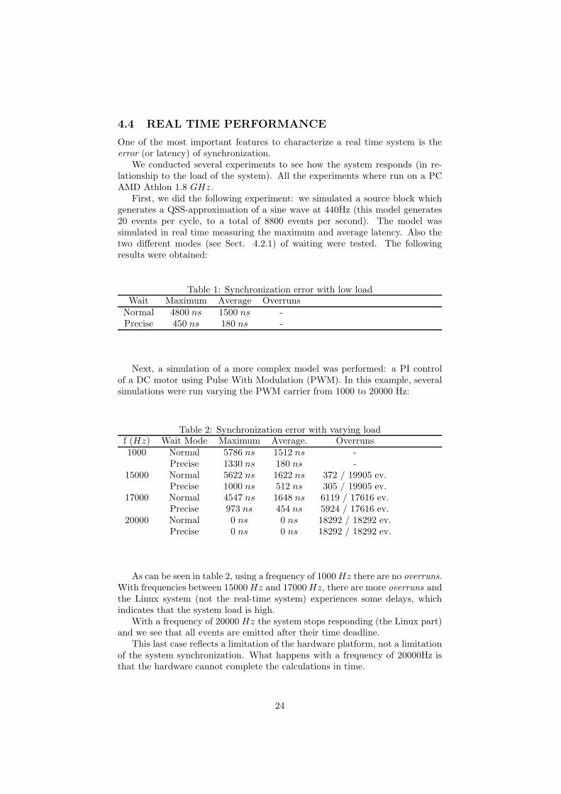
First, we did the following experiment: we simulated a source block whichgenerates a QSS-approximation of a sine wave at 440Hz (this model generates20 events per cycle, to a total of 8800 events per second). The model wassimulated in real time measuring the maximum and average latency. Also thetwo different modes (see Sect. 4.2.1) of waiting were tested. The followingresults were obtained:

Table 1: Synchronization error with low loadWait Maximum Average Overruns

Normal 4800 ns 1500 ns -Precise 450 ns 180 ns -

Next, a simulation of a more complex model was performed: a PI controlof a DC motor using Pulse With Modulation (PWM). In this example, severalsimulations were run varying the PWM carrier from 1000 to 20000 Hz:

Table 2: Synchronization error with varying loadf (Hz) Wait Mode Maximum Average. Overruns1000 Normal 5786 ns 1512 ns -

Precise 1330 ns 180 ns -15000 Normal 5622 ns 1622 ns 372 / 19905 ev.

Precise 1000 ns 512 ns 305 / 19905 ev.17000 Normal 4547 ns 1648 ns 6119 / 17616 ev.

Precise 973 ns 454 ns 5924 / 17616 ev.20000 Normal 0 ns 0 ns 18292 / 18292 ev.

Precise 0 ns 0 ns 18292 / 18292 ev.

As can be seen in table 2, using a frequency of 1000 Hz there are no overruns.With frequencies between 15000 Hz and 17000 Hz, there are more overruns andthe Linux system (not the real-time system) experiences some delays, whichindicates that the system load is high.

With a frequency of 20000 Hz the system stops responding (the Linux part)and we see that all events are emitted after their time deadline.

This last case reflects a limitation of the hardware platform, not a limitationof the system synchronization. What happens with a frequency of 20000Hz isthat the hardware cannot complete the calculations in time.

24

4.5 INTERRUPT LATENCY

To measure the interrupt latency the following procedure was used.A PowerDEVS model was created (Fig. 10) which generates hardware in-

terrupts and then captures back these interrupts, measuring the period of timebetween the generation of the signal provoking the interrupt and the capture ofthe interrupt by the handler.

For that purpose, we used the PC Parallel port. One of the pins on theparallel port (STO) is in charge of generating interrupts. This pin was wired toa data pin, thus generating a hardware interrupt every time that the data pingoes from a low state (0 V) to a high state (5V). The model stores the timeat which a 1 is written to the data pin (high state), and the time at which theinterrupt handler of the parallel port is run. The difference between these twotimes is an upper bound of the interrupt latency of the system (in fact, thatdifference includes also the time needed to write on the parallel port and theelectrical transients).

Figure 10: Interrupt Latency tester model

Running this experiment on the same hardware (PC AMD 1.8Ghz) we ob-tained an upper bound on the interrupt latency of about 20µs.

5 EXAMPLES

This section describes two examples that show different features of PowerDEVS.

5.1 RIPPLE VS FREQUENCY IN A BUCK CIRCUIT

Figure 11 represents a DC-DC converter circuit known as Buck Circuit.The presence of the switch introduces hybrid behavior to the system.The goal of the experiments is to analyze the dependence of the ripple am-

plitude on the switching frequency. In this example we used the following pa-rameters L1 = L2 = 0.1mH, C = 20µF, Rl = 10Ω and U = 12V.

Figure 12 shows the PowerDEVS model of the circuit, made entirely withatomic blocks from the PowerDEVS library. The switch is commanded by a

25

+

-

L1 L2

C RlU

Figure 11: Buck Circuit

PWM signal. The remaining blocks implement source, static functions andintegrators based on QSS methods.

The frequency of the triangular carrier was chosen in a way that increments2000Hz in each simulation. The “RunScilab Job” block increments the Scilabvariable n after each simulation and calculates the ripple amplitude in steadystate. This amplitude is saved in the array u(n).

Figure 12: Buck Circuit Model

After 100 simulations (in which the frequency goes from 2000 to 200000 Hz),we can plot the results directly in Scilab (see Fig. 13).

It must be noticed that 100 simulations of this hybrid system (with very quickcommutations) were run, and thanks to the efficiency of the QSS methods totreat this kind of problems, the experiment only took about 13 seconds (whilein Matlab/Simulink it takes about a minute).

26

Figure 13: Ripple vs. Frequency

5.2 DC MOTOR CONTROL IN REALTIME

This example shows the real time asynchronous control of a DC Motor. For thispurpose, we used a small DC drive moving an old PC mouse wheel acting as anencoder (see Fig.14). Each time the wheel moves a small angle, a pulse is sentto the bit STO of the parallel port, which triggers an interrupt in the PC. Themotor is fed by an amplifier, implemented with a transistor and a filter takingthe on–off voltage from a data pin of the parallel port.

Figure 14: Motor and mouse (encoder)

The control system is composed of the following subsystems (see Fig. 15):

• The Motor Speed block detects and counts the interrupts generated by theencoder to estimate the motor speed.

27

• This estimation is compared to the reference speed (the block WSum4calculates the difference or error).

• In base of this error a Proportional-Integral (PI) Control is applied, usingQSS discretization.

• The control signal (previously saturated to avoid over-modulation) is pulsewidth modulated.

• The PWM signal (calculated in the Comparator1 block), is sent syn-cronized to the parallel port.

Figure 15: Proportional Control Model

The whole control system of Fig.15 was built using blocks from the Pow-erDEVS library, except the model that estimates the motor speed based on thenumber of interrupts it receives per second.

Figure 16 shows the reference speed signal while Fig. 17 shows the speedmeasured by the control system.

-10

0

10

20

30

40

50

60

70

80

90

0 2 4 6 8 10

Figure 16: Reference speed

6 CONCLUSIONS AND FUTURE WORK

We introduced and described a general purpose tool for DEVS simulation. Weillustrated its use in hybrid system simulation, where it shows the most impor-

28

0

10

20

30

40

50

60

70

80

0 2 4 6 8 10

Figure 17: Measured speed

tant facilities and advantages compared with existing simulation software.Besides the user friendly environment and the simplicity it offers to different

kinds of users, PowerDEVS has a new way of managing the simulation timeadvance which allows to implement simulations synchronized with a real–timeclock and with the possibility of handling interrupts in an easy fashion. In thatway, it can directly implement hybrid asynchronous QSC controllers (as it wasdone in the example of the DC motor control).

However, PowerDEVS is not only a tool for hybrid system simulation andcontrol. As we mentioned before, it is a general purpose DEVS simulator andtaking into account that its use is very simple, it results appropriated for edu-cation.

Compared with other existing DEVS simulation environments, the mainadvantage of PowerDEVS is the conveninet user interface and the simplicityto implement continuous and hybrid system simulations based on the family ofQSS methods. Also the possibility to running simulations under a real timeoperating system (RTAI) and the communication with Scilab are remarkablefeatures.

When it comes to future work, an immediate goal is to finish the migration ofPowerDEVS source code from Visual Basic to C++ with QT libraries. At themoment, only the model editor needs to be translated. After that, the completeenvironment would run under different platforms without the need of Windowsemulators (the current version of the PowerDEVS model editor uses the WineWindows Emulator to run under Linux and RTAI).

The incorporation of visual programming tools can also improve the atomicmodel edition. At the moment, users can build complex models by couplingsimpler ones (unless they are good programmers). An alternative way to buildcomplex atomic models is with the help of graphical tools, like Simulink State-flows. A tool that translates graphical formalisms into atomic PowerDEVSC++ code might facilitate the generation of new atomic blocks. If such a toolis developed (as a separated program) it can be integrated with PowerDEVS ina straightforward manner because of its user–configurable menu features.

Finally, a project is worked on at the ETH Zurich to automatically translateModelica models into PowerDEVS models (based on QSS approximations). Thecompletion of that goal shall permit to drastically increase the modeling capa-bility of PowerDEVS, also giving Modelica users the possibility of implementingQSS simulations.

29

REFERENCES

[1] Michael Barabanov. A linux-based realtime operating system. Master’sthesis, New Mexico Institute of Mining and Technology, New Mexico, 1997.

[2] Daniel Bovet and Marco Cesati. Understanding the Linux Kernel. O’ Reilly,2002.

[3] S. Campbell, J. Chancelier, and Ramine Nikoukhah. Modeling and Simu-lation in Scilab/Scicos. Springer, 2006.

[4] Francois Cellier and Ernesto Kofman. Continuous System Simulation.Springer, New York, 2006.

[5] Francois Cellier, Ernesto Kofman, Gustavo Migoni, and Mario Bortolotto.Quantized state system simulation. In Proceedings of SummerSim 08 (2008Summer Simulation Multiconference), Edinburgh, Scotland, 2008.

[6] Hyup Cho and Young Cho. DEVS–C++ Reference Guide. The Universityof Arizona, 1997.

[7] J.B. Filippi, M. Delhom, and F. Bernardi. The JDEVS EnvironmentalModeling and Simulation Environment. In Proceedings of IEMSS 2002,volume 3, pages 283–288, 2002.

[8] Claude Ed. Gomez. Engineering and scientific computing with Scilab.Birkhauser, Boston, 1999. Includes bibliography and index.

[9] Hermann Hartig, Robert Baumgartl, Martin Borriss, and Claude-JoachimHaman. Drops: Os support for distributed multimedia applications. In EW8: Proceedings of the 8th ACM SIGOPS European workshop on Support forcomposing distributed applications, pages 203–209, New York, NY, USA,1998. ACM.

[10] Dan Hildebrand. An architectural overview of qnx. In Proceedings of theWorkshop on Micro-kernels and Other Kernel Architectures, pages 113–126, Berkeley, CA, USA, 1992. USENIX Association.

[11] http://www.acims.arizona.edu/SOFTWARE/devsjava3.0/setupGuide.html.Devsjava.

[12] http://www.mathworks.com/products/rtw/. Real-time workshop 7.0.

[13] Tag Gon Kim. DEVSim++ User’s Manual. C++ Based Simulation withHierarchical Modular DEVS Models. Korea Advance Institute of Scienceand Technology, 1994.

[14] Harold Klee. Simulation of Dynamic Systems with MATLAB and Simulink.CRC, 2007.

[15] E. Kofman. Quantization–Based Simulation of Differential Algebraic Equa-tion Systems. Simulation, 79(7):363–376, 2003.

[16] E. Kofman. A Third Order Discrete Event Simulation Method for Contin-uous System Simulation. Latin American Applied Research, 36(2):101–108,2006.

30

[17] Ernesto Kofman. Quantized-State Control. A Method for Discrete EventControl of Continuous Systems. Latin American Applied Research,33(4):399–406, 2003.

[18] Ernesto Kofman. Discrete Event Simulation of Hybrid Systems. SIAMJournal on Scientific Computing, 25(5):1771–1797, 2004.

[19] P. Mantegazza, E. L. Dozio, and S. Papacharalambous. Rtai: Real timeapplication interface. Linux J., page 10.

[20] Gustavo Migoni and Ernesto Kofman. Linearly Implicit Discrete EventMethods for Stiff ODEs. Latin American Applied Research, 2009. In press.

[21] Jim Nutaro. Adevs (a discrete event system simulator).

[22] Esteban Pagliero and Marcelo Lapadula. Herramienta Integrada de Mod-elado y Simulacion de Sistemas de Eventos Discretos. Diploma Work.FCEIA, UNR, Argentina, September 2002.

[23] H. Vangheluwe. DEVS as a Common Denominator for Multi-formalism Hy-brid Systems Modelling. In IEEE International Symposium on ComputerAided Control System Design, pages 129–134, Anchorage, Alaska, 2000.

[24] Gabriel Wainer. Cd++: a toolkit to develop devs models. Software: Prac-tice and Experience, 32(13):1261–1306, 2002.

[25] Gabriel Wainer, Gaston Christen, and Alejandro Dobniewski. DefiningDEVS Models with the CD++ Toolkit. In Proceedings of ESS2001, pages633–637, Marseille, France, 2001.

[26] Christof Wehner. Tornado and VxWorks. BoD, 2006.

[27] Karim Yaghmour. Adaptive domain environment for operating systems.2002. www.opersys.com/adeos/.

[28] Karim Yaghmour. Building a real-time operating systems on topof the adaptive domain environment for operating systems. 2003.www.opersys.com/adeos/.

[29] B. Zeigler. Theory of Modeling and Simulation. John Wiley & Sons, NewYork, 1976.

[30] B. Zeigler and S. Vahie. Devs formalism and methodology: unity of concep-tion/diversity of application. In Proceedings of the 25th Winter SimulationConference, pages 573–579, Los Angeles, CA, 1993.

[31] Bernard Zeigler and Hessam Sarjoughian. Introduction to DEVS Model-ing and Simulation with JAVA: A Simplified Approach to HLA-CompliantDistributed Simulations. Arizona Center for Integrative Modeling and Sim-ulation. Available at http://www.acims.arizona.edu/.

[32] Bernard P. Zeigler, Herbert Praehofer, and Tag Gon Kim. Theory of Mod-eling and Simulation - Second Edition. Academic Press, 2000.

31