Poverty and Tropical Deforestation by Smallholders in Forest Margin Areas: Evidence from Central 

Sulawesi, Indonesia     

 

Sunny W.H. Reetz Stefan Schwarze 

Bernhard Bruemmer  

sreetz@gwdg.de; sschwar1@gwdg.de; bbruemm@gwdg.de    

Department of Agricultural Economics and Rural Development Platz der Goettinger Sieben 5 37073 Goettingen, Germany 

  

  Selected Paper prepared for presentation at the International Association of Agricultural Economists (IAAE) Triennial Conference, Foz do Iguaçu, Brazil, 18‐24 August, 2012.     Copyright 2012 by Sunny W.H. Reetz, Stefan Schwarze and Bernhard Bruemmer.   All rights reserved.  Readers may make verbatim copies of this document for non‐commercial purposes by any means, provided that this copyright notice appears on all such copies.   

Abstract The negative impacts of climate change have made poverty and deforestation topics of heightened interest within global community discussions in recent years. Our study contributes to the debate over the links between poverty and deforestation by providing an alternative approach from the village level perspective, whilst broadening the range of poverty measures based on poverty proxies and subjective well-being (SWB). We use a beta regression in our empirical model. Our results suggest that there is a non-linear relationship between SWB, as well as other poverty proxies, and deforestation. We found that objective and subjective poverty measures yielded contrasting results. Keywords

Deforestation; Subjective well-being; Poverty proxies

2

1. Introduction

One key priority of national and international development policies is to combat

poverty in developing countries. Ideally, poverty reduction should not have negative

external effects which might aggravate global warming. However, these goals have been

difficult to achieve. An example from South East Asia shows that poverty was reduced

considerably over the last three decades, yet regional deforestation rates are the highest in

tropical regions (Wunder, 2001). Indonesia had an average annual deforestation rate of

0.71 million hectares per year between 2000 and 2005, second only to Brazil during this

period (World Research Institute, 2010). Here, the Indonesian agricultural sector, which is

the driver of deforestation, has remained the backbone of the rural economy and

contributed significantly to poverty alleviation (Tacconi & Kurniawan, 2006; Thorbecke &

Jung, 1996). This further demonstrates the difficulties in disconnecting economic

development from negative environmental effects, in this case deforestation.

The causes of deforestation are manifold and include logging, mining and the

establishment of plantations or pastures. The agents of deforestation also vary depending

on these activities. As an example, large land holders are responsible for the expansion of

pasture land for beef production into previously forested areas in Brazil (Fearnside, 2005;

Lele et al., 2000). Deforestation conducted by smallholders is the proximate cause of at

least 50 percent of deforestation in tropical forests (Barraclough & Ghimire, 2000).

Therefore, our study focuses on deforestation by smallholders, although later we

aggregate the analysis up to the village level.

Two mainstreams can be identified within the growing literature that analyses the

link between poverty and deforestation by smallholders. Some have perceived that

agricultural expansion carried out by smallholders is triggered by poverty (Coxhead,

Shively, & Shuai, 2002; Deininger & Minten, 1999; Dennis et al., 2005; Geist & Lambin,

2001; Godoy et al., 1997; Kerr et al., 2004; Maertens, Zeller, & Birner, 2006; Rudel &

Roper, 1997) whilst other scholars have argued that poverty has no direct link to

deforestation (Chomitz, 2007; Dasgupta, Deichmann, Meisner, & Wheeler, 2005; Khan &

Khan, 2009; Wunder, 2001; Zwane, 2007). Accordingly, the question of whether poverty

causes deforestation has been the subject of debate during the last decades.

The link between poverty and deforestation is complex as it depends on factors

such as geographical location and institutional arrangements, and is further complicated

by the existence of different theoretical approaches towards poverty, each of which utilise

3

many methods to measure poverty. These different approaches and methods might explain

why the existing literature regarding the poverty-deforestation link contains contradictory

results. As an example, Khan (2009), using satellite imaging and poverty mapping in Swat

district, Pakistan found that there is no empirical evidence that poverty is associated with

forest degradation. Dasgupta (2005), using absolute poverty indices from consumption

expenditure, found that there are moderate correlations between poverty and deforestation

rates in three developing countries (Cambodia, Lao PDR, and Vietnam), and that they are

correlated at the district level for Cambodia, and at the provincial level for Lao PDR.

Although poverty is a complex phenomenon, most studies have used generalised

approaches towards poverty and, therefore, failed to distinguish the specific effects which

different elements of poverty have on deforestation (Dasgupta, et al., 2005; Deininger &

Minten, 1999; Godoy, et al., 1997). Moreover, most studies apply monetary measures or

use consumption approaches to assess poverty at a household level (Dasgupta, et al.,

2005; Zwane, 2007).

Our study provides an alternative approach towards the poverty-deforestation link

from the village level perspective. In our opinion, the drivers of deforestation will be more

clearly observable at a higher level than households because deforestation is strongly

associated with collective poverty and economic diversity at the village level (Angelsen &

Wunder, 2003; Dewi, Belcher, & Puntodewo, 2005), and many socio-demographic factors

(e.g. population density, infrastructures) and geophysical factors (e.g. elevation, slope)

have few variations across households.

The effects of different elements of poverty on deforestation have not previously

been explored. In particular, very little research on subjective well-being (SWB) has been

done in developing countries, and only a few studies have applied SWB as a proxy of

poverty (Kingdon & Knight, 2005; Pradhan & Ravallion, 2000; Ravallion & Lokshin,

2002). Our study contributes to the debate over the links between poverty and

deforestation. The use of poverty proxies including SWB assessments serves to capture

the multidimensionality of poverty and therefore help to formulate improved policy

suggestions to reduce future forest losses. However, there are some shortcomings of SWB

assessments in terms of: accuracy, reliability (as a result of respondents interpreting

questions differently), and different perceptions among the neighbouring respondents. The

shortcomings of the objective approach are related to data availability and quality, as well

4

as the issue of different perceptions of what constitute basic needs and minimum

requirements (Angelsen & Wunder, 2003; Expert Group on Poverty Statistics, 2006).

This paper examines the relationship between poverty and deforestation in a

region of tropical forest in the vicinity of Lore Lindu National Park in Central Sulawesi,

Indonesia. This park hosts many collections of endemic species, however this region is

also characterised by high rates of poverty and deforestation. Forest cover decreased by

4.8 percent from 2001 to 2007 whilst 59.1 percent of households were living below the

international poverty line of 2 USD per capita per day in 2007 (Van Edig, Schwarze, &

Zeller, 2010). Smallholders are the major agents of forest degradation in this area

(Maertens, et al., 2006; Steffan-Dewenter et al., 2007). The link between poverty and

deforestation in this region, in particular the effects of different elements of poverty on

deforestation, require consideration in order to devise sustainable development policies

which simultaneously reduce poverty, preserve the long-term functioning of the forests

and protect peoples’ livelihoods.

Our results suggest that there is a non-linear relationship between deforestation and

SWB as well as other proxies of poverty. The relationships found differ depending on

whether poverty is viewed from a subjective or objective perspective. The subjective

assessment indicates that only the extreme poor and rich villages have high rate of

deforestation. In contrast, the relative poverty assessment as an objective view shows no

empirical evidence that poverty increases the deforestation rate. Moreover, additional

proxies derived from particular elements of poverty dimensions also within an objective

view have an unclear pattern; variables might increase or decrease the deforestation rate.

High illiteracy rates and less access to markets increase deforestation rates, whilst the

availability of electricity in a village increases the deforestation rate. Nevertheless, from

the overall subjective perspective, between 2001 and 2007 the improvement of village

well-being encouraged a reduction in the deforestation rate.

The remainder of the paper is organised as follows: Section 2 provides our

conceptual framework which underlines the links between poverty and deforestation.

Section 3 explains the data and methods, with particular attention to the data-collection

process as well as coverage and accuracy of data. In Section 4, we provide and discuss our

results, and in Section 5 we conclude the paper.

5

2. Conceptual Framework

Before discussing potential linkages between poverty and deforestation, we clarify

the key terms. According to the definition of the Intergovernmental Panel on Climate

Change (IPCC), deforestation is the permanent or temporary removal of forest cover and

conversion to a non-forest land use. This includes natural events such as landslides and

forest fires, as well as human activities such as shifting cultivation, clear-cut logging, and

other types of land conversion from forest to non-forest use (Erasmi, Twele, Ardiansyah,

Malik, & Kappas, 2004; Noble et al., 2000). Poverty, meanwhile, is a more

multidimensional phenomenon, and its measurement is typically linked to many variables,

including many dynamic components. One commonly accepted definition appropriately

reflects the complexity of poverty; the World Bank describes poverty as a social condition

of chronic insecurity resulting from malfunctioning of the economic, ecological, cultural,

and social systems, which causes a group or class of people to lose the capacity to adapt

and survive and to live below minimum levels required to satisfy their needs (World

Bank, 2001). Thus, poverty relates to situations in which people are unable to meet

economic, social, and other standards of well-being. However, the definition of poverty is

incomplete without including gender inequality and environmental issues as well (OECD,

2001). Such a broad definition of poverty is open to subjective interpretation, because

each case of poverty occurs within a particular context.

We adopt here the terms “objective approach” and “subjective approach”. For both

approaches we must consider the technical issues involved in methods used to measure

poverty. The objective approach has used some standard techniques to measure poverty.

These techniques employ different indicators of well-being such as: poverty lines, head

count indices with either a monetary approach or a food energy intake method (FEI), or

the direct calorie intake method (DCI) with a consumption approach. These approaches

have been used to estimate the incidence of poverty within a community, either at a

regional or national level using a household as the unit of observation (Coudouel,

Hentschel, & Quentin, 2002). To apply the aforementioned poverty measures analysis to

our 80 sampled villages, however, would have been financially costly and research

intensive for this project. As an alternative to monetary or consumption indicators of well-

being, we employ poverty proxies and Subjective Well-Being (SWB). Subjective methods

use a conceptual definition of poverty better suited to our specific research context, which

will be explained further towards the end of this section. It is important that our outsiders’

view of poverty is informed also by the opinions of community members in order to

6

define what they believe constitutes being poor. Perspectives of local people obtained

using SWB have until now been left unexplored and only a few studies have applied SWB

as a proxy of poverty in developing countries (Kingdon & Knight, 2005; Pradhan &

Ravallion, 2000; Ravallion & Lokshin, 2002). Both the objective and subjective

perspective approaches have some drawbacks. The shortcomings of SWB assessments are

in terms of: accuracy, reliability (as a result of respondents interpreting questions

differently), and different perceptions among the neighbouring respondents. The

shortcomings of the objective approach are related to data availability and quality, as well

as the issue of different perceptions of what constitute basic needs and minimum

requirements (Angelsen & Wunder, 2003; Expert Group on Poverty Statistics, 2006).

Spatial overlap between high incidences of poor rural communities and forest cover

areas have been found by some studies (Chomitz, Buys, De Luca, Thomas, & Wertz-

Kanaounnikoff, 2007; Sunderlin, Resosudarmo, Rianto, & Angelsen, 2000) as well as

potential links between poverty and deforestation (Coxhead, Shively, & Shuai, 2002;

Deininger & Minten, 1999; Dennis et al., 2005; Geist & Lambin, 2001; Godoy et al.,

1997; Kerr et al., 2004; Maertens, Zeller, & Birner, 2006; Rudel & Roper, 1997). There

may be reciprocal causality between deforestation rates and their influencing factors. For

example, villages which contain more motorcycles tend to have higher deforestation rates

in the initial study period. However this does not mean that such communities have higher

rates of deforestation as a result of their greater wealth. An alternative explanation might

be that more villagers could afford motorcycles as a result of deforestation-derived wealth.

In order to avoid reversal effects between deforestation and explanatory variables

occurring in the model, we must set an assumption of unidirectional causal relationship. In

practice, we circumvented the possibility of reciprocal causality by including factors that

influenced deforestation from the initial period only. Here, we determine that the

deforestation rate, as our dependent variable, has a unidirectional causal relationship to the

explanatory variables.

Although our study focuses on a natural tropical forest in which deforestation is

primarily caused by agricultural expansion of smallholders, we used the village as the unit

of observation in order to link poverty and deforestation. We believe that this is

advantageous because in our opinion drivers of deforestation will be more observable at a

higher level than households. Furthermore deforestation is strongly associated with

collective poverty and economic diversity at the village level (Angelsen & Wunder, 2003;

7

Dewi, et al., 2005). Meanwhile, many variables such as socio-demographic factors (e.g.

population density, infrastructures) and geophysical factors (e.g. elevation, slope) are

largely uniform between households. Thus, the influence of poverty on deforestation rates

should become more apparent at an aggregated level.

We aim to understand the relationship between various elements of poverty and

deforestation, as well as to explore significant effects of particular aspects of poverty on

the deforestation process at the village level. These particular aspects of poverty include;

demographics, cultural and social systems, technology, health and sanitation, economy,

education, gender inequality, environmental issues, and geophysical conditions. For each

of the different elements, a set of proxies is required. For example the number of

secondary schools and the illiteracy rate is used as a proxy for education. However, we

must recognise that a given proxy might also simultaneously reflect other aspects of

poverty. The SWB index is used to capture the respondents’ view of their situation.

Besides recognising the multidimensionality of poverty, the use of poverty proxies and

SWB assessments helps to formulate improved policy implications to reduce future forest

losses.

3. Data and Methodology

a. Study Area

The study area is located in central Sulawesi, Indonesia, and contains both

lowland and mountainous forests with an altitude ranging from 200 to 2,610 meters

above sea level. The study area is approximately 7,500 square kilometres, which

includes 2,200 square kilometres of the Lore Lindu National Park (LLNP) (Erasmi &

Priess, 2007). Most of the area is characterised by a humid tropical climate. 78 percent

of the 80 villages surveyed lie within the largest portion of rainforest cover. The LLNP

hosts many collections of endemic species that are of great biodiversity and natural

conservation importance. However agricultural expansion threatens the integrity of the

park’s biodiversity.

From 2001 to 2007, the population increased by 14.1 percent, equivalent to a

mean annual growth rate of 2.2 percent. Although this population growth rate is only

slightly higher than at the provincial level (2.1 percent), it is significantly greater than

the national level (1.3 percent). Such a high growth rate might indicate that this area is

facing population pressure. The main indigenous groups residing in the area are the

8

Kaili and Kulawi. However, the share of non-indigenous people is relatively high,

comprising 32 percent of the total population. Furthermore the largest ethnic group is

the Buginese, who originated from the South Sulawesi province.

Farming is the major occupation in the area with 86.8 percent of households

completely dependent on agricultural activities. Earnings from non-agricultural

activities are low, providing financial support for only 13.2 percent of households. In

general, access to central markets has improved considerably since 2001, whilst the

share of villages that are accessible by motorcycle has increased from 85 percent to

100 percent. Especially in the northern part of the region, the increase in the number of

roads and road quality improvements has reduced the amount of time required for

local people to reach the central market in the provincial capital Palu.

b. Data

Geo-referenced data were collected from various sources. These data include

land use and topographic information for the study area. The land use information was

derived from Landsat ETM+ scenes and was compiled into a 100 x 100 meter grid

resolution in a GIS (Geography Information System) programme. For more details on

the geo-referenced data see Erasmi and Priess (2007). We calculated the deforestation

rate as the dependent variable in our model. Using village boundary data, we were able

to determine the magnitude of deforestation for each village. The deforestation rate for

each village was calculated by dividing the area of surrounding land that had been

deforested between 2001 and 2007 by the total forest area in 2001. Furthermore, we

included topographic information for each selected village obtained by calculating the

average elevation and slope.

The 80 study villages were selected from the total of 119 using a stratified

random sample (Zeller, Schwarze, & Van Rheenen, 2002). Village socioeconomic

data was obtained by conducting two surveys based on standardised questionnaires

during the same year. We also obtained secondary data from village censuses and

other documents. The survey comprised interviews in the form of a panel discussion,

which were conducted by a team of two enumerators who interviewed the village

leader and other village representatives in each of the selected villages. Each panel

consisted of 4 to 6 representatives who were appointed due to their good knowledge of

their village.

9

The questionnaires covered issues of village demographics, land use, agricultural

technology and markets, land and labour, livestock, national park and conservation

issues, infrastructure, income and wealth, El Nino-related drought, and future

challenges. Moreover, to capture the multidimensionality of poverty, we generated

data relating to poverty in three different ways. First, we assessed the relative poverty

of the villages in the research area using a poverty assessment tool that was developed

in a previous survey at the household level in 2005 (Van Edig, et al., 2010). In that

study, two sets of 15 poverty indicators were tested to provide a robust poverty tools

assessment (PATs) that were used to predict households’ daily per capita expenditures.

Next, estimations of daily per capita expenditures were utilised to predict the

distribution of poor households in the community. From those two sets of poverty

indicators, we selected three indicators, namely education, health and sanitation and

housing dimensions, that could be applicable at the village level. These three

indicators were most applicable to and suitable for our village survey because they

were easy to assess by enumerators and village representatives.

The first indicator education level for a given household was whether or not they

include at least one family member who had graduated from high school. The second

indicator, health and sanitation, characterises households based on whether or not they

own a private pit toilet. The last indicator, housing, characterises households on the

basis of whether or not they have exterior walls built from concrete. We define

households as poor if they report favourable conditions for no more than one of these

three poverty indicators, whereas we define better-off households as those benefitting

from favourable ratings for at least two indicators. These classifications were chosen

based on our field observations which suggested that households who possess two of

these indicators are considered significantly better-off, while households considered to

be poor possess one indicator and the poorest lack all three indicators. Questions about

these aforementioned criteria were asked during the panel discussion with village

representatives. By subtracting the percentage of better-off households from the total

percentage of households, we estimated the percentage of poor households in the

village.

Secondly, we assessed SWB as another proxy for poverty. SWB is measured by

asking respondents to evaluate their livelihoods through self-completed reports which

measure their emotional responses, domain satisfaction, and global judgements of life

10

satisfaction (Diener & Seligman, 2004; Hoorn, 2008). SWB measurements vary from

single-item scales to multi-item scales and more advanced measures (Hoorn, 2009),

such as the so-called Experience Sampling Method (ESM) or Ecological Momentary

Assessment (EMA) (Scollon, Kim-Prieto, & Diener, 2003) and Day Reconstruction

Method (DRM) (Kahneman, Krueger, Schkade, Schwarz, & Stone, 2004; Kahneman

& Krueger, 2006). Using SWB allowed us to measure local peoples’ perspectives on

their own well-being. Despite the importance of SWB and its increasing prominence

within economics literature, very little research on SWB has been done in developing

countries. Previous SWB research has been done in (Pradhan & Ravallion, 2000)

Nepal and Jamaica; (Lokshin, Umapathi, & Paternostro, 2003; Ravallion & Lokshin,

2002)) Russia; (Bookwalter & Dalenberg, 2004; Kingdon & Knight, 2005; Neff,

2006)) South Africa; (Graham & Pettinato, 2001) Latin America and Russia; and

(Appleton & Song, 2008) urban China. Moreover, only a few of these studies have

applied SWB as a proxy of poverty aspects (Kingdon & Knight, 2005; Neff, 2006;

Pradhan & Ravallion, 2000; Ravallion & Lokshin, 2002). While these studies apply

SWB at the household level, we attempt to apply SWB at the village level. In our

study, we asked village representatives to rate their village’s welfare relative to that of

their neighbouring villages on a single-item scale. Respondents were presented with an

image of a ladder with 10 steps, of which the lowest step represents the poorest

villages and the tenth step represents the wealthiest villages. Meanwhile our survey

asked respondents to indicate the wealth of their village in comparison to these two

extremes for 2001 and 2007 using the same ladder. We then calculated the changes

between wealth ranks on the ladder over the 6 year interlude. A positive value

indicates that the village became relatively wealthier, and vice versa. Lastly, we

included selected variables to use as additional proxies of poverty: access to economic

resources, agricultural technology, gender inequality, environmental issues, and

income diversity1.

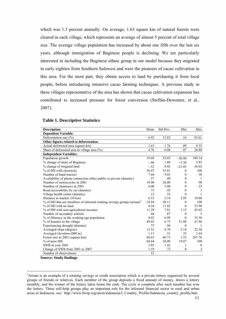
Table 1 presents the descriptive statistics for study area. The deforestation rate in

the research area was almost 7 percent between 2001 and 2007, which is equivalent to

approximately, 1.2 percent annually. This rate is slightly lower than the national rate,

1 Although we sampled 80 villages, we observed only 52 in order to concentrate on the pure effects of poverty on deforestation. We therefore excluded villages with dependent variables (deforestation rate) less than zero which resulted by policy interventions such as local afforestation programs. We also excluded those villages with dependent variables with values greater than one because these deforestation rates were the result of changes in village size between 2001 and 2007 and therefore inaccurate. Moreover, since we used percentage change in irrigated land as one of our variables in a model, we excluded villages without irrigated land.

11

which was 1.3 percent annually. On average, 1.63 square km of natural forests were

cleared in each village, which represents an average of almost 5 percent of total village

size. The average village population has increased by about one fifth over the last six

years, although immigration of Buginese people is declining. We are particularly

interested in including the Buginese ethnic group in our model because they migrated

in early eighties from Southern Sulawesi and were the pioneers of cacao cultivation in

this area. For the most part, they obtain access to land by purchasing it from local

people, before introducing intensive cacao farming techniques. A previous study in

three villages representative of the area has shown that cacao cultivation expansion has

contributed to increased pressure for forest conversion (Steffan-Dewenter, et al.,

2007).

Table 1. Descriptive Statistics Description: Mean Std Dev. Min MaxDependent Variable: Deforestation rate (%) 6.92 12.82 .16 83.01Other figures related to deforestation: Actual deforested area (square km) 1.63 1.76 .09 9.35Share of deforested area in village area (%) 4.76 6.08 .07 28.80Independent Variables: Population growth 19.68 32.03 50.90 189.14% change of share of Buginese .46 1.88 5.30 5.85% change of irrigated land .52 8.42 21.05 36.02% of HH with electricity 56.47 33.81 0 100Number of hand tractors 7.44 9.03 0 38Availability of phone connection either public or private (dummy) .37 .49 0 1Number of motorcycles in 2001 19.00 24.00 0 98Number of chainsaws in 2001 4.00 5.00 0 25Road accessibility by car (dummy) .73 .45 0 1Village health centre (dummy) .12 .32 0 1Distance to market (10 km) 6.53 2.14 2.95 10.80% of HH that are members of informal rotating savings groups (arisan)2 24.94 30.11 0 100% of HH with no land 4.24 11.02 0 53.98% of HH with non-agricultural incomes 11.29 7.81 1.15 43.02Number of secondary schools .44 .87 0 5% of illiteracy in the working age population 4.02 6.99 0 35.50% of females in the village 49.03 6.75 31.80 67.96Experiencing drought (dummy) .75 .44 0 1Averaged slope (degree) 13.52 4.70 2.14 22.30Averaged elevation (000 m) 1.11 .31 .35 1.64Forest size in 2001 (square km) 60.65 60.73 1.53 267.76% of poor HH 68.64 24.00 19.87 100SWB in year 2001 3.85 1.42 1 8Change of SWB from 2001 to 2007 1.19 .72 0 3Number of observations 52

Source: Study findings

2Arisan is an example of a rotating savings or credit association which is a private lottery organized by several groups of friends or relatives. Each member of the group deposits a fixed amount of money, draws a lottery monthly, and the winner of the lottery takes home the cash. The cycle is complete after each member has won the lottery. These self-help groups play an important role for the informal financial sector in rural and urban areas in Indonesia. see: http://www.bwtp.org/arcm/indonesia/I_Country_Profile/Indonesia_country_profile.htm

12

The study area is characterised by use of basic technologies and has limited access

to public services. Over half of village households have electricity. Almost three

quarters of roads within the observed villages are accessible by car, and over a quarter

of villages have a phone connection either from a public phone, a mobile phone, or a

fixed line. The average village has more than 90 motorcycles, which are the most

important means by which people and agricultural goods are transported, and therefore

they are used as the proxy for market access. More than 10 percent of the villages

surveyed have health centres. Regarding economic properties, income diversification

is low and only about 11 percent of households have non-agricultural income sources.

Almost a quarter of the village population has access to an informal rotating credit

association (arisan). Physical distances to the central markets vary between 30 and 110

kilometres, with most of the roads in poor condition. In terms of education, less than

half the villages have a secondary school and 4 percent of working age people are

illiterate. The gender demographic is almost balanced. Almost three quarters of the

villages in this study area have experienced drought between 2001 and 2007, the

occurrence of which might indirectly make people more vulnerable to poverty. Most

lands are situated on steep slopes at high elevations, and remaining forest cover within

villages varies from less than 2 to almost 270 square km. People defined as poor

comprise, on average, more than two thirds of village populations. In regard to SWB

measures, the average village in 2001 had a value greater than 3, on a scale of 1 to 10,

with a range from 1 to 8 recorded. On average SWB scores improved between 2001

and 2007.

c. Econometric Model

To estimate the influence of poverty on deforestation, we apply a beta regression

model. The dependent variable in our model is the rate of deforestation between 2001 and

2007, which ranges between values of 0 and 1. Since the dependent variable is a rate or

proportion, OLS (Ordinary Least Squares) is inappropriate and inaccurate due to the

skewed distribution of the residuals. Moreover, a rate or proportion dependent variable

often violates the OLS’ assumptions of normality and homoscedasticity as values tend to

be concentrated within the middle range, and less so in the lower and upper limits.

Therefore a beta distribution was considered for the analysis of the dependent variable

(Cribari-Neto & Zeleis, 2010; Ferrari & Cribari-Neto, 2004; Smithson & Verkuilen,

2006).

13

Beta distribution is a flexible distribution which can accommodate a uniform,

unimodal, or bimodal distribution of points that can either be symmetrical or skewed

(Paolino, 2001). The standard beta density is expressed as:

; , гг г

1 ,0 1 (1)

where p,q > 0 and Г(.) denotes the gamma function. The mean and variance of y are,

respectively,

1.

To obtain a regression structure that contains a precision parameter and the mean of

response, Ferrari & Cribari-Neto (2004) proposed an alternative parameterisation with μ

= p/(p+q) and = p+q, which can be written as:

;, г г г

1 ,0 1 (2)

where the mean and variance of y are, respectively:

1

.

The parameter is known as the precision parameter since, for fixed μ, the larger the the

smaller the variance of y; 1 is a dispersion parameter. The precision parameter is

assumed to be constant and the mean is related to a set of covariates through a linear

predictor with unknown coefficients and a link function (Cribari-Neto and Zeileis, 2010).

The link function for a beta regression is represented as follows:

∑ (3)

where β = (β1, …,βk)┬ is a k x 1 vector of unknown regression parameters (k < n), xtti =

(xt1, … , xik) ┬ is the vector of k regressors (or independent variables or covariates) and ηt

is a linear predictor. Finally, g(.) : (0,1) →ΙR is a link function, which is strictly increasing

and twice differentiable. There are two advantages in using a link function. First, both

sides of the regression equation assume values in the real line when a link function is

applied to μt. Second, it gives practitioners flexibility in choosing the function that best

fits. For instance, one can use some useful link functions g(.) such as the logit

specification, the probit function, and the log-log link (Cribari-Neto & Zeleis, 2010;

14

Ferrari & Cribari-Neto, 2004). Further discussions of link functions can be found in

McCullagh (1989).

The estimation of beta regression is performed by maximum likelihood. The

interpretation of the estimation results is less straightforward than normal linear models

(OLS) but the regression parameters are interpretable in terms of the mean of y (the

dependent variable). Nonetheless, maximum likelihood estimation using a beta

distribution can yield more accuracy and precision than OLS or even GLM (Generalised

Linear Model) when dealing with proportional data, as demonstrated by practitioners

from other disciplines. (Paolino, 2001; Ferrari and Cribari-Neto, 2004; and Smithson and

Verkuilen, 2006). Smithson and Verkuilen (2006) in particular have used comparisons of

several alternative approaches to show that the beta regression model performs markedly

better than potentially viable alternatives. Although GLM can be used as an alternative to

beta regression, beta regression is the more appropriate because it can deal better with the

distribution of our data (Paolino, 2001).

4. Empirical Results and Discussion

Before performing our analysis, we illustrated the relationship between SWB and

the rate of deforestation using kernel density estimation (Figure 1).

Figure 1. Subjective Well Being (SWB) vs. Deforestation Rates

Source: Study findings

The form of the kernel density estimation suggests that there is a non-linear relationship

between both variables. Deforestation decreases as the SWB value increases from 1 to 2

Kernel regression, bw = .5, k = 6

Grid points1 8

3.54565

73.6902

Deforestation rate

SWB values in 2001

15

and it reaches a peak at 4. Subsequently, the deforestation rate decreases again and

remains constant between 5 and 6, at which point it increases rapidly. For this reason, we

introduced the SWB variable as a polynomial in our model.3

Table 2. Beta Regression Estimations

Variable: Estimated Marginal Effects (Mfx) at x

Coef. Coef.(Mfx) SE (Mfx)

Population growth

% Change of share of Buginese

% Change of irrigated land . 025 *** .001 *** .000

% of HH with electricity .009 *** 3e-04 *** .000

Number of hand tractors

Availability of phone connection either public or private (dummy)

Number of motorcycles in 2001

Number of chainsaws in 2001

Road accessibility by car (dummy)

Village health service (dummy)

Distance to market (10 km) .179 *** .006 *** .001

% of HH that are members of informal rotating savings groups (arisan) .021 *** .001 *** .000

% of HH with no land .011 *** 3e-04 ** .000

% of HH with non-agricultural incomes

Number of secondary schools

% of illiteracy in the working age population .030 *** .001 *** .000

% of females in the village .079 *** .003 *** .000

Experiencing drought (dummy)

Averaged slope (degree) .217 *** .007 *** .000

Averaged elevation (000 m) 1.871 *** .060 *** .010

Forest size in 2001 (km2) .006 *** 2e-04 *** .000

% of poor HH .026 *** .001 *** .000

SWB in 2001 cubic .200 *** See Figure 3

SWB in 2001 squared 2.634 *** See Figure 3

SWB in 2001 10.584

*** See Figure 3

Change of SWB from 2001 to 2007 .221 *** .007 *** .002

Constant 6.962 ***

/ln phi() 5.157 ***

Number of observed villages

52

Prob> chi2 0.00

Phi () 173.633

Log Likelihood 150.088

Parameter 17

*,**,*** Significant at the 10%, 5%, and 1% level, respectively. Source: Study findings

3We have also checked for linearity of other poverty proxy variables. The results indicate that those variables are non-linear. However, adding a square term for those variables does not improve the beta regression model.

16

The results of the beta regression model, which analyses the influence of poverty

on deforestation, are presented in Table 2. Because the interpretation of the estimated

coefficients is not straightforward compared normal linear models, we also present

marginal effects. The marginal effect is the change in the deforestation rate resulting from

a single unit change in the corresponding explanatory variable, keeping all other variables

at the mean. To specify our model we adopted a general to specific approach, which is

superior to a specific to general approach. The LR test shows that the effects of

insignificant variables of the full model are equal to zero4, and therefore their inclusion

did not improve the model. In the beta regression, the precision parameter with its identity

link, showed as ln phi(), is presented on a logarithmic scale to ensure that it remains

positive. The high significance (1%) of the ln phi() variable in our model indicates that

the precision coefficients can be treated as a full model parameter instead of a nuisance

parameter (Zeleis, Cribari-Neto, Grün, Simas, & Rocha, 2011).

All variables in our estimated model are highly significant at the 1 percent level

except for “marginal effect of percentage household with no land”, which is significant at

the 5 percent level. Our model indicates that certain elements of poverty such as

technology, economy, education, gender and geographical conditions significantly

influence the rate of deforestation, while other elements such as demographics, cultural

and social system and environmental issues have no significant influence on the

deforestation rate. Closer inspection of technology reveals that each element of

technology has a different influence on the deforestation rate. Increases in the percentage

of irrigated land reduce the deforestation rate; between 2001 and 2007 a 1 percent increase

led to a reduction of the deforestation rate by 0.001. The irrigated land is typically used

for wetland-paddy rice cultivation, which requires a large amount of labour. As a result, it

may be that less labour is available to encroach on forest lands. In contrast, a 10%

increase in the percentage of households with electricity increases the deforestation rate

by 0.002. Apparently, having electricity facilitates peoples’ access to technology and

information via radio and television.

We found that greater distances to the market increase deforestation. The marginal

effects show that a 10 kilometre increase in distance to market increases deforestation

rates by 0.006. This suggests that physical barriers to market access do not impede

deforestation activities. An increase in other socio-economic variables appear to lower the

4 LR test (Prob> chi2) with ρ-value = 0.871

17

deforestation rate. For example if the share of village households in arisan and the share

of landless households in a village increases by 10 percentage points, the rate of

deforestation decreases by 0.01 and 0.003 respectively. As formal financial institutions are

not available in most villages, becoming a member of an arisan gives rural people

alternative means of obtaining cash than by cutting the surrounding forests. Cash received

from an arisan could also be used to intensify agricultural production, which might in turn

lead to lower forest conversion rates. The finding that a higher share of landless

households is negatively correlated with deforestation suggests that poor households are

not the direct actors who open up forests for agricultural uses.

Our empirical model shows that the deforestation rate increases by 0.01 for every

10 percent rise in the share of illiterate working age people. Uneducated villagers are

highly dependent on agricultural employment as they have few other work options.

Moreover, the only chance to improve their well-being is to increase their share of

agricultural land by encroaching into forests. A high proportion of female inhabitants

negatively affects the deforestation rate. If the share of females in a village increases by 1

percentage point, the deforestation rate is reduced by 0.003. This confirms that forest

margin agricultural expansion activities are dominated by male farmers.

Geophysical factors such as steep slopes and high elevation reduce the

deforestation rate. The deforestation rate decreases by 0.007 for every 1 degree slope

increase and decreases by 0.006 for every one hundred meter increase in elevation.

Notice that the change in the deforestation rate is more responsive to elevation than slope.

It is not possible to grow any agricultural crops above a certain elevation, although we

found that farmers were still able to establish a number of cacao plots in extremely steep

areas. This should be considered when formulating policy recommendations to promote

land conservation in steep slope areas for the purpose of reducing instances of landslides

and soil erosion. Forest size in 2001 was taken as a control variable in our model, and it

was found that larger forests in 2001 had higher deforestation rates; for every 10

kilometre square increase, the deforestation rate increases by 0.002.

Other proxies that consider multiple aspects of poverty include: share of poor

households in a village (objective approach), and the SWB, which also has a highly

significant influence on the deforestation rate. A higher share of poor households in the

village reduces the rate of deforestation; if the share of poor households in a village

increases by 10 percent, the deforestation rate is reduced by 0.01. This shows that people

from

Furt

pres

mar

resp

betw

decr

mar

shap

are r

200

Furt

defo

shar

bein

view

Add

dec

illit

ava

m poor hous

thermore, b

sent Figure

ginal effect

pect to the

ween defore

reases until

ginal impac

ped function

responsible

When w

1 to 2007,

ther, a one

orestation ra

re of poor

ng perceptio

w provides n

ditional obj

crease the d

teracy rates

ailability of

seholds are

ecause the S

2 to illustr

t of the SW

SWB valu

estation an

l a SWB of

ct between

nal form. T

for high de

we look at t

we find tha

e level we

ate by 0.00

households

on suggest d

no empirica

jective pove

deforestatio

s and less

f electricity

not the dir

SWB enters

rate the im

WB variable

ue in 2001

d SWB in

f 4 is reach

SWB in 2

This shape i

eforestation

the changes

at an increa

ll-being im

07. Howeve

in a villag

different res

al evidence t

Figure 2. M

erty proxie

on rate. As

access to

y in a vill

rect actors w

s the regres

mpact of thi

is a derivat

(dMu/dSW

2001. Fig

hed in 200

2001 and th

indicates th

rates.

s in wealth

ase in wealt

mprovement

er, proxies

ge (an obje

sults. The re

that poverty

Marginal E

Source: Stu

s have uncl

we can se

markets in

lage increa

who open u

sion in form

s variable o

tive of the p

WB), which

gure 2 show

1, beyond

he deforesta

hat the extre

correspond

th ranking

t within th

of differen

ective meas

elative pove

y increases t

Effects of SW

udy findings

lear pattern

ee from the

ncrease defo

ses defores

up forests fo

m of a polyn

on the defo

polynomial

h reflects th

ws that the

which it in

ation rate h

eme poor an

ding to cha

reduces the

he last six

nt aspects o

ure), and th

erty assessm

the deforest

WB

ns; variables

e beta regre

forestation r

station. On

or agricultu

nomial func

orestation r

function (M

he real rela

e deforestat

ncreases aga

hence follow

nd the rich

anges in SW

e deforestat

years redu

of poverty

he subjectiv

ment as an o

tation rate.

s might inc

ession mod

rates, altho

n the contr

18

ural uses.

ction, we

rate. The

Mu) with

ationship

tion rate

ain. The

ws a U-

villages

WB from

ion rate.

uces the

such as:

ve well-

objective

crease or

del, high

ough the

rary, the

19

subjective assessment provides clear evidence that extreme poor and rich villages have

high rates of deforestation.

5. Conclusions and Policy Implications

Although much previous research has investigated the link between poverty and

deforestation, the majority used simplistic definitions of poverty and focused on the

household level. Our study contributes to the debate on the link between poverty and

deforestation by presenting multifaceted appraisals of poverty and thus more

comprehensively considering links between particular aspects of poverty and their effects

on deforestation. Further our approach towards the poverty-deforestation link uses the

village level perspective, because few variations exist across households. Thus, the drivers

of deforestation are more observable at a higher level than households. Moreover, by

focusing on the village level, we are able to analyse a wider range of poverty dimensions,

by using SWB, as well as other poverty proxies.

Our results suggest that there is a non-linear relationship between deforestation

and SWB as well as other proxies of poverty. Moreover, the results show different

linkages between deforestation and poverty depending on the poverty dimensions

considered. A number of poverty proxies such as technology, economy, education, gender

and geographical conditions were found to significantly influence the rate of

deforestation. For other elements, related to demographics, or the cultural and social

system, we found no significant impact on the deforestation rate. Nevertheless, among the

identified drivers of deforestation, those related to technologies had contrasting effects on

deforestation rates; an increase in the percentage of irrigated land had a negative impact,

although electricity availability increases the deforestation rate. Regarding economic

factors, we found that longer distances to the market increase deforestation, but other

economic proxies such as higher proportions of village households which are members of

rotation savings groups (arisan) and higher shares of landless households reduced the

deforestation rate. Among the variables related to education, only the share of illiteracy in

the working age population affected the rate of deforestation, where higher illiteracy rates

led to higher deforestation. A higher proportion of female village inhabitants reduces the

deforestation rate. Geophysical factors such as steep slopes and high elevation reduced the

deforestation rate.

By considering different dimensions of poverty, we found that objective and

subjective poverty measures yielded contrasting results. The objective relative poverty

20

assessment provides no empirical evidence that poverty affects the deforestation rate.

Further objective measures of aspects of poverty show contrasting patterns; particular

variables might increase or decrease the deforestation rate. On the contrary, subjective

assessments clearly indicate that extreme poor and rich villages have high rates of

deforestation. Although wealthier villages had higher deforestation rates during 2001, by

2007 increases in well-being had decreased the rate of deforestation in this region. Our

findings highlight for the benefit of future research on links between poverty and

deforestation that a holistic consideration of poverty is required, as different approaches

and measures yield contrasting results.

Give that improvements in village well-being appears to eventually lower rates of

deforestation, policy measures aimed at reducing poverty may also reduce deforestation.

However, the non-linear relationship between initial SWB and deforestation suggests that

there remain trade-offs between forest conservation and poverty reduction. Policy makers

should therefore consider such trade-offs, and aim to improve education and training on

environmentally-friendly agricultural practices, such as agro-forestry systems and terrace

construction in highland areas to reduce landslides and soil erosion, which are

particularly important for highland deforested areas. Another option would be to help and

encourage informal rotating savings groups (arisan), which help farmers manage their

financial resources in order to intensify agricultural production, since this leads to long-

term forest preservation. Investment in irrigation is another policy option since it has a

forest-conserving effect; nonetheless cost-benefit analyses are required in order to assess

the viability of such investments.

21

References

Angelsen, A., & Wunder, S. (2003). Exploring the Forest-Poverty Link: Key Concepts, Issues and Research Implications (Occasional Paper): Center for International Forestry Research (CIFOR).

Appleton, S., & Song, L. (2008). Life Satisfaction in Urban China: Components and Determinants. World Development, 36(11), 2325-2340.

Barraclough, S. L., & Ghimire, K. B. (2000). Agricultural Expansion and Tropical Deforestation – Poverty, International Trade and Land Use. London: Earthscan Publications.

Bookwalter, J. T., & Dalenberg, D. (2004). Subjective Well-Being and Household Factors in South Africa. Social Indicators Research, 65, 333-353.

Chomitz, K. M. (2007). At Loggerheads: Agricultural Expansion, Poverty Reduction, and Environment in the Tropical Forests. Wahington, D.C.: The World Bank.

Chomitz, K. M., Buys, P., De Luca, G., Thomas, T. S., & Wertz-Kanaounnikoff, S. (2007). At Loggerheads? Agricultural Expansion, Poverty Reduction, and Environment in the Tropical Forests: The World Bank.

Coudouel, A., Hentschel, J. S., & Quentin, T. W. (2002). Poverty Measurement and Analysis A Sourcebook for Poverty Reduction Strategies (Vol. 1): World Bank.

Coxhead, I., Shively, G., & Shuai, X. (2002). Development Policies, Resource Constraints, and Agricultural Expansion on The Philippine Land Frontier. Environment and Development Economics 7(2), 341-363.

Cribari-Neto, F., Zeleis, A., 2010. Beta Regression in R. Journal of Statistical Software, 34, 1-22.

Dasgupta, S., Deichmann, U., Meisner, C., & Wheeler, D. (2005). Where is the Poverty? Environment Nexus? Evidence from Cambodia, Lao PDR, and Vietnam. World Development, 33(4), 617-638.

Deininger, K. W., & Minten, B. (1999). Poverty, Policies, and Deforestation: The Case of Mexico. Economic Development and Cultural Change, 47(2), 313-344.

Dennis, R. A., Mayer, J., Applegate, G., Chokkalingam, U., Colfer, C. J. P., Kurniawan, I., et al. (2005). Fire, People and Pixels: Linking Social Science and Remote Sensing to Understand Underlying Causes and Impacts of Fires in Indonesia. Human Ecology, 33(4), 465-504.

Dewi, S., Belcher, B., & Puntodewo, A. (2005). Village Economic Opportunity, Forest Dependence, and Rural Livelihoods in East Kalimantan, Indonesia. World Development, 33(9), 1419-1434.

Diener, E., & Seligman, M. E. P. (2004). Beyond Money: Toward An Economy of Well-Being. Psychological Science in the Public Interest, 5(1), 1-31.

Erasmi, S., & Priess, J. A. (2007). Satelite and Survey Data: A Multiple Source Approach to Study Regional Land-Cover/ Land-Use in Indonesia. In F. Dickmann (Ed.), Geovisualisierung in der Humangeographie (Kartographische Schriften 13 ed., pp. 101-114). Bonn: Kirschbaum Verlag.

Erasmi, S., Twele, A., Ardiansyah, M., Malik, A., & Kappas, M. (2004). Mapping Deforestation and Land Cover Conversion at the Rainforest Margin in Central Sulawesi, Indonesia. EARSeL eProceedings, 3(3), 388-397.

Expert Group on Poverty Statistics. (2006). Compendium of Best Practices in Poverty Measurement (Rio Group). Rio de Janeiro.

Fearnside, P., 2005. Deforestation in Brazilian Amazonia: History, Rates, and Consequences. Conservation Biology, 19, 680-688.

22

Ferrari, S., & Cribari-Neto, F. (2004). Beta Regression for Modelling Rates and Proportions. Journal of Applied Statistics, 31(7), 799-815.

Geist, H., & Lambin, E. (2001). What Drives Tropical Deforestation: A Meta-analysis of Proximate and Underlying Causes of Deforestation Based on Subnational Case Study Evidence (LUCC Report Series No. 4).

Godoy, R., O'Neill, K., Groff, S., Kostishack, P., Cubas, A., Demmer, J., et al. (1997). Household Determinants of Deforestation by Amerindians in Honduras. World Development, 24(6), 977-987.

Graham, C., & Pettinato, S. (2001). Happiness, Market, and Democracy: Latin America in Comparative Perspective. Journal of Happiness Studies, 2(237-268).

Hoorn, A. A. J. v. (2008). A Short Introduction to Sujective Well-Being: Its Measurement, Correlates and Policy Uses. In OECD (Ed.), Statistics, Knowledge and Policy 2007: Measuring and Fostering the Progress of Societies. Paris: OECD Publishing.

Hoorn, A. A. J. v. (2009). Measurement and Public Policy Uses Subjective Well-Being (Working Paper No. 09-110). Nijmegen: Nijmegen Center for Economics (NiCE) Radboud University Nijmegen.

Kahneman, D., Krueger, A., Schkade, D., Schwarz, N., & Stone, A. A. (2004). A Survey Method for Characterizing Daily Life Experience: The Day Reconstruction Method. Science, 306(5702), 1776-1780.

Kahneman, D., & Krueger, A. B. (2006). Developments in the Measurement of Subjective Well-Being. Journal of Economic Perspectives, 20, 3-24.

Kerr, S., Pfaff, A. S. P., Cavatassi, R., Davis, B., Lipper, L., Sanchez, A., et al. (2004). Effects of Poverty on Deforestation: Distinguishing Behavior from Location (ESA Working Paper): Agricultural and Development Economics Division.

Khan, S. R., & Khan, S. R. (2009). Assessing Poverty–Deforestation Links: Evidence from Swat, Pakistan. Ecological Economics, 68(10), 2607-2618.

Kingdon, G. G., & Knight, J. (2005). Subjective Well-Being Poverty Versus Income Poverty and Capabilities Poverty?

Lele, U., Viana, V., Verissimo, A., Vosti, S., Perkins, K., & Husain, S. A. (2000). Brazil-Forests in the Balance of Conservation with Development: The World Bank.

Lokshin, M., Umapathi, N., & Paternostro, S. (2003). Robustness of Subjective Welfare Analysis in Poor Developing Country: Madagascar 2001: The World Bank.

Maertens, M., Zeller, M., & Birner, R. (2006). Sustainable Agricultural Intensification in Forest Frontier Areas. Agricultural Economics 34(2), 197-206.

McCullagh, P., & Nelder, J. (1989). Generalized Linear Models (second ed.). London: Chapman & Hall.

Neff, D. F. (2006). Subjective Well-Being, Poverty and Ethnicity in South Africa: Insights from an Exploratory Analysis. Social Indicators Research, 80(2), 313-341.

Noble, I., Apps, M., Houghton, R., Lashof, D., Makundi, W., Murdiyarso, D., et al. (2000). Implications of Different Definitions and Generic Issues. In T. R. Watson, I. Noble, B. Bolin, N. H. Ravindranath, D. J. Verardo & D. J. Dokken (Eds.), Land Use, Land-Use Change, and Forestry: Cambridge University Press.

OECD. (2001). The DAC Guidelines. Poverty Reduction. Paris. Pradhan, M., & Ravallion, M. (2000). Measuring Poverty Using Qualitative Perceptions of

Consumption Adequacy. The Review of Economics and Statistics, 82(3), 462-471. Ravallion, M., & Lokshin, M. (2002). Self-rated Economic Welfare in Russia. European

Economic Review, 46, 1453-1473. Rudel, T., & Roper, J. (1997). The Paths to Rain Forest Destruction: Crossnational Patterns of

Tropical Deforestation, 1975-90. World Development, 25(1), 53-65. Scollon, C. N., Kim-Prieto, C., & Diener, E. (2003). Experience sampling: Promises and

Pitfalls, Strengths and Weaknesses. Journal of Happiness Studies, 4(1), 304-326.

23

Smithson, M., Verkuilen, J., 2006. Supplemental Material for a Better Lemon Squeezer? Maximum-Likelihood Regression with Beta-Distributed Dependent Variables. Psychological Methods, 11, 54-71.

Steffan-Dewenter, I., Kessler, M., Barkmann, J., Bos, M. M., Buchori, D., Erasmi, S., et al. (2007). From the Cover: Tradeoffs between Income, Biodiversity, and Ecosystem Functioning during Tropical Rainforest Conversion and Agroforestry Intensification. Proceedings of the National Academy of Sciences, 104(12), 4973-4978.

Sunderlin, W., Resosudarmo, I. A. P., Rianto, E., & Angelsen, A. (2000). The Effect of Indonesia's Economic Crisis on Small Farmers and Natural Forest Cover in the Outer Islands (Occasional Paper).

Tacconi, L., & Kurniawan, I. (2006). Forests, Agriculture, Poverty and Land Reform: the Case of the Indonesian Outer Islands (EMD Working Paper No. OP11): The Australian National University.

Thorbecke, E., & Jung, H. (1996). A Multiplier Decomposition Method to Analyse Poverty Alleviation. Development Economics, 48, 279-300.

Van Edig, X., Schwarze, S., & Zeller, M. (2010). The Robustness of Indicator Based Poverty Assessment Tools in Changing Environments - Empirical Evidence from Indonesia. In T. Tscharntke, C. Leuschner, E. Veldkamp, H. Faust, E. Guhardja & A. Bidin (Eds.), Tropical Rainforests and Agroforests under Global Change: Ecological and Socio-economic Valuations (Environmental Science and Engineering) (pp. 191-211): Springer.

World Bank. (2001). Attacking Poverty (World Development Report 200/01). Washington D.C.

World Research Institute. (2010). Forest Cover Loss in Indonesia, 2000-2005: The Starting Point for the Norwegian Billion to Reduce Deforestation. from http://www.wri.org/map/forest-cover-loss-indonesia-2000-2005-starting-point-norwegian-billion-reduce-deforestation

Wunder, S. (2001). Poverty Alleviation and Tropical Forests: What Scope for Synergies? World Development, 29(11), 1817-1833.

Zeleis, A., Cribari-Neto, F., Grün, B., Simas, A. B., & Rocha, A. V. (2011). Beta Regression. Retrieved from http://cran.r-project.org/web/packages/betareg/betareg.pdf

Zeller, M., Schwarze, S., & Van Rheenen, T. (2002). Statistical Sampling Frame and Methods Used for the Selection of Villages and Households in the Scope of the Research Program on Stability of Rainforest Margins in Indonesia (STORMA) (STORMA Discussion Paper Series Sub-program A on Social and Economic Dynamics in Rainforest Margins No. 1). Goettingen: Georg-August-Universitaet.

Zwane, A. (2007). Does poverty constrain deforestation? Econometric evidence from Peru. Journal of Development Economics, 84(1), 330-349.

24

Appendix 1. The Full Model Estimations

Variable: Full Model

Population growth .001

% Change of share of Buginese .013

% Change of irrigated land .030 ***

% of HH with electricity .008 ***

Number of hand tractors .006

Availability of phone connection either public or private (dummy) .148

Number of motorcycles in 2001 .005

Number of chainsaws in 2001 .007

Road accessibility by car (dummy) .371

Village health service (dummy) .019

Distance to market (10 km) .193 ***

% of HH that are members of informal rotating savings groups (arisan) .021 ***

% of HH with no land .015 ***

% of HH in non-agriculture incomes .003

Number of secondary schools .046

% of illiteracy in the working age population .003 ***

% of females in the village .070 ***

Experiencing drought (dummy) .028

Averaged slope (degree) .227 ***

Averaged elevation (000 m) 1.838 ***

Forest size in 2001 (km2) .005 *

% of poor HH .027 ***

SWB in 2001 cubic .202 ***

SWB in 2001 squared 2.642 ***

SWB in 2001 10.442 ***

Change of SWB from 2001 to 2007 .295 ***

Constant 6.650 ***

/ln phi() 5.248 ***

Number of observed villages

52

Prob> chi2 0.00

Phi() 190.287

Log Likelihood 153.543

Parameter 28

*,**,*** Significant at the 10%, 5%, and 1% level, respectively. Source: Study findings