Postpr int - DiVA portaluu.diva-portal.org/smash/get/diva2:852147/FULLTEXT01.pdf · Postpr int This is the accepted version of a paper published in International Journal of Computer

http://www.diva-portal.org

Postprint

This is the accepted version of a paper published in International Journal of Computer Mathematics.This paper has been peer-reviewed but does not include the final publisher proof-corrections or journalpagination.

Citation for the original published paper (version of record):

von Sydow, L., Toivanen, J., Zhang, C. (2015)

Adaptive finite differences and IMEX time-stepping to price options under Bates model.

International Journal of Computer Mathematics, 92: 2515-2529

http://dx.doi.org/10.1080/00207160.2015.1072173

Access to the published version may require subscription.

N.B. When citing this work, cite the original published paper.

Permanent link to this version:http://urn.kb.se/resolve?urn=urn:nbn:se:uu:diva-262065

June 26, 2015 International Journal of Computer Mathematics paperdraftbates˙final

To appear in the International Journal of Computer MathematicsVol. 00, No. 00, Month 20XX, 1–16

Adaptive finite differences and IMEX time-stepping to price options

under Bates model

L. von Sydowa∗, J. Toivanenb,c, C. Zhanga

aDepartment of Information Technology, Uppsala University, Sweden; bInstitute for

Computational and Mathematical Engineering (ICME), Stanford University, USA;cDepartment of Mathematical Information Technology, University of Jyvaskyla, Finland

(Received 00 Month 20XX; accepted 00 Month 20XX)

In this paper we consider numerical pricing of European and American options under the Batesmodel, a model which gives rise to a partial-integro differential equation. This equation is discretizedin space using adaptive finite differences while an IMEX scheme is employed in time. The sparse linearsystems of equations in each time-step are solved using an LU-decomposition and an operator splittingtechnique is employed for the linear complementarity problems arising for American options. Theintegral part of the equation is treated explicitly in time which means that we have to perform matrix-vector multiplications each time-step with a matrix with dense blocks. These multiplications areaccomplished through fast Fourier transforms. The great performance of the method is demonstratedthrough numerical experiments.

Keywords: Option pricing; numerical methods; Bates model, adaptive finite differences, IMEXtime-stepping

2010 AMS Subject Classification: 65M06, 91G60

1. Introduction

The model for the underlying asset in the seminal paper [5] by Black and Scholes in 1973on option pricing is a geometrical Brownian motion. A few years later in [20] Merton addslog-normally distributed jumps to this model as empirical studies on stock price seriessuggest existence of jumps. In the end of 1980s it was widely recognized that the constantvolatility assumption of the Black–Scholes model is unrealistic for many underlying assetsand several models with stochastic volatility were proposed. Probably the most popularamong these models is the one proposed by Heston in [11]. Bates combined the Mertonjump-diffusion model and the Heston stochastic volatility model in his 1996 paper [4].As this model by Bates is reasonably realistic for many underlying assets we consideroption pricing based on it in this paper.

Under the Bates model a parabolic partial-integro differential equation (PIDE) can bederived for the prices of European options. The variables of this PIDE are the asset valueand its variance. The underlying partial differential operator is of convection-diffusiontype while the integral operator integrates over all values in the asset value direction.For the price of American options, a linear complementarity problem (LCP) can beformulated with the same underlying partial-integro differential operator. We consider

∗Corresponding author. Email: [email protected]

1


pricing European and American options by employing finite difference discretizationsfor differential operators and a suitable quadrature for the integral operator. The mostcommonly used finite differences lead to a sparse block tridiagonal matrices while thequadrature leads to block diagonal matrices with full diagonal blocks.

The efficient discretization and solution techniques derived for these option pricingproblems is discussed in the following. Implicit time discretizations require the solutionof a system with a coefficient matrix having full diagonal blocks at each time step. Theiterative methods considered in [33], [27] can solve these problems reasonably efficiently.Alternatively the ADI-type operator splitting method in [3] gives an efficent approximatesolution procedure. Still avoiding an implicit treatment of the integral operator canlead to a simpler and more efficient solution procedure. Cont and Voltchkova considerin [8] the IMEX-Euler method which treats the integral operator explicitly and thedifferential operator implicitly. This method is only first-order accurate in time. TheIMEX-midpoint [18], [17] and IMEX-CNAB [28], [30] methods are similar, but second-order accurate methods in time. In this paper, we employ the IMEX-CNAB method.The explicit treatment of the integral operator leads to multiplications by a matrix withfull blocks. These can be performed efficiently using fast Fourier transforms (FFT); see[2], [10], for example.

The IMEX time discretizations require the solution of a two-dimensional convection-diffusion-reaction type problem at each time step. Several different efficient solution andapproximation methods have been proposed for these problems. These include multigridmethods [7], [22], preconditioned iterations [40], [25], and directional operator splittingmethods [13], [16]. Here we employ a direct solver based on LU decomposition. Recentlythis approach was shown to be efficient and convenient for these problems in [30]. ForAmerican options an LCP with the same operator needs to be solved at each time step.The LCP can be approximated and solved using various methods including an operatorsplitting method [12], [15], [30], penalty methods [39], [9], and multigrid methods [7], [22],[26], [14], [35]. Here we use the operator splitting method to approximate the solutions ofLCPs as it is accurate and easy to implement. Futhermore, it leads to systems of linearequations which can be solved using standard efficient solution methods.

Finite difference discretizations have been used dominantly for the Bates model; see[6], [34], [29], [30]. In [21], a finite element discretization was used. The main topic ofthis paper is the choice of a good nonuniform finite difference grid. The grid should beas coarse as possible to save computational time, but fine enough to reach the desiredaccuracy. Here such a grid is constructed adaptively. We employ the approach describedin [23], [24] for a multi-dimensional Black–Scholes model and the Heston model. The basicidea is to estimate the spatial discretization error on a coarse grid based on the orderof convergence of the discretization and then by employing this error estimate constructa fine grid. As the grid used for error estimation can be fairly coarse the computionalcost of the error estimation is small while the obtained fine grid is nearly optimal. Analternative, more elaborate approach would be to use a goal oriented adjoint equationbased method described in [19]. For more discussion on adaptive discretizations see thebook [1].

The outline of the paper is the following. We begin by describing the Bates modeland the resulting PIDE and LCP for European and American options in Section 2. Fora given grid the spatial discretization is constructed in Section 3. The temporal IMEXdiscretization and the use of FFT to evaluate the integrals in each time-step is describedin Section 4. The adaptive construction of spatial grids is introduced in Section 5. Theoperator splitting method for American options is given in Section 6. Numerical resultsand conclusions are presented in Sections 7 and 8, respectively. Acknowledgments end

2


the paper.

2. Mathematical model

Under the Bates model [4] the asset value St and the instantaneous variance Vt satisfythe stochastic differential equations

dSt = (r − q − λξ)Stdt+√VtStdW

1t + (J − 1)StdN,

dVt = κ(θ − Vt)dt+ σ√VtdW

2t ,

(1)

where r is the risk free interest rate, q is the dividend yield, λ is the intensity of thePoisson process N , the jump J has a log-normal distribution

f(J ) =1√

2πδJexp

(−(lnJ − (γ − δ2/2)

)22δ2

),

where γ and δ define the mean and variance of the jump and ξ is given by ξ = exp(γ)−1.The mean-reversion level of the variance is θ and κ is the rate of reversion to this meanlevel and finally W1 and W2 are Wiener processes with the correlation ρ.

The price u of a European option issued on an asset following the process defined in(1) can be computed by solving the following PIDE

∂u(s, v, τ)

∂τ=

1

2vs2∂

2u(s, v, τ)

∂s2+

1

2vσ2∂

2u(s, v, τ)

∂v2+ ρσvs

∂2u(s, v, τ)

∂s∂v

+ (r − q − λξ)∂u(s, v, τ)

∂s+ κ(θ − v)

∂u(s, v, τ)

∂v

− (r + λ)u(s, v, τ) + λ

∫ ∞0

u(J s, v, τ)f(J )dJ = Lu,

(2)

where τ = T − t is the time to expiry. The initial condition for (2) is defined by thepayoff function Φ for the option, which for a European call option is

u(s, v, 0) = Φ(s) = max(s−K, 0). (3)

For the American options we must take into account the possibility for early exercisewhich leads to the following LCP:

∂u∂τ + Lu ≥ 0,

u ≥ Φ,

(u− Φ)(∂u∂τ + Lu

)= 0,

(4)

with the initial condition (3) for an American call option. We will denote the free bound-ary by sf that separates the stopping region where u = Φ and the continuation region

defined by ∂u∂τ + Lu = 0.

3


3. Spatial discretization

We will discretize the spatial operator Lu on a structured but nonequidistant grid (si, vj),0 ≤ si ≤ smax, 0 ≤ vj ≤ vmax with ms grid-points in s and mv grid-points in v. Theboundary conditions used for the European call option are

u(0, v, τ) = 0,

u(smax, v, τ) = smaxe−qτ −Ke−rτ ,

∂u(s, vmax, τ)

∂v= 0,

and for the American call option

u(0, v, τ) = 0,

u(smax, v, τ) = max(smaxe−qτ −Ke−rτ , smax −K),

∂u(s, vmax, τ)

∂v= 0.

For the parameter settings we consider we have u(smax, v, τ) = smax−K for the Americanoption.

We discretize the derivatives in (2) using centered, second-order finite differences ona nonequidistant grid, see [23], [24]. For the derivatives in the v-directions that do notvanish at v = 0, we use one-sided first-order finite differences there. The discrete approx-imation of the integral term in (2) is evaluated by first making a transformation fromthe original computational grid si to an equidistant grid xk. Let

I =

∫ ∞0

u(Js, v, τ)f(J)dJ =

∫ ∞−∞

u(x+ z, v, τ)f(z)dz,

where x = log s, z = logJ , u(z, v, τ) = u(ez, v, τ) and f(z) = ezf(ez). Then we define anew variable ζ = z + x and obtain at x = xk the integral

Ik =

∫ ∞−∞

u(ζ, v, τ)f(ζ − xk)dζ =

∫ xmax

xmin

u(ζ, v, τ)f(ζ − xk)dζ

+

∫ xmin

−∞u(ζ, v, τ)f(ζ − xk)dζ +

∫ ∞xmax

u(ζ, v, τ)f(ζ − xk)dζ = I(1)k + I

(2)k + I

(3)k .

(5)

We compute the first part of (5) using the trapezoidal quadrature rule on an equidistantgrid in x with spacing ∆x and mx grid-points in [xmin, xmax] giving

I(1)k =

∫ xmax

xminu(ζ, v, τ)f(ζ − xk)dζ ≈ ∆x

∑mx

j=1 u(ζj , v, τ)f(ζj − xk)

− ∆x2

(u(xmin, v, τ)f(xmin − xk) + u(xmax, v, τ)f(xmax − xk)

).

4


The second part I(2)k can be approximated by

I(2)k =

∫ xmin

−∞u(ζ, v, τ)f(ζ − xk)dζ ≈ u(xmin)

1

2

(1 + erf

(xmin − xk − (γ − δ2/2)√

2δ

))

Finally we compute I(3)k where we use u(s, v, τ) ≈ se−qτ −Ke−rτ , s ≥ smax for European

options and u(s, v, τ) ≈ s−K, s ≥ smax for American options. For European options weobtain

I(3)k =

∫ ∞xmax

u(ζ, v, τ)f(ζ − xk)dζ ≈sk2eγ−qτ

(1− erf

(xmax − xk − γ − δ2/2√

2δ

))

− K

2e−rτ

(1− erf

(xmax − xk − (γ − δ2/2)√

2δ

)).

and similarly for American options we obtain

I(3)k =

∫ ∞xmax

u(ζ, v, τ)f(ζ − xk)dζ ≈sk2eγ(

1− erf

(xmax − xk − γ − δ2/2√

2δ

))

− K

2

(1− erf

(xmax − xk − (γ − δ2/2)√

2δ

)).

4. Temporal discretization and Fast Fourier Transforms (FFTs)

The discretization of the differential operator in (2) leads to a sparse matrix A with 9non-zero elements per row while the numerical quadrature rule for the integral part leadsto a block-diagonal matrix J with full diagonal blocks. Due to the different structuresof the matrices we employ an implicit/explicit (IMEX) scheme in time which treats thediscrete differential operator A implicitly and J explicitly. This way we avoid having tosolve a dense linear system of equations each time-step.

First we employ the IMEX-Euler scheme [8], four time-steps using the time-step ∆t2

un+1/2 =∆t

2Aun+1/2 +

∆t

2Jun + un , n = 0, 1

2 , 1,32 , (6)

which can be written as(I − ∆t

2A

)un+1/2 =

∆t

2Jun + un , n = 0, 1

2 , 1,32 . (7)

For the remaining time-steps we use IMEX Crank-Nicolson/Adams-Bashforth (IMEX-CNAB) scheme [28], with the time-step ∆t

un+1 =∆t

2A(un+1 + un

)+

∆t

2J(3un − un−1

)+ un , n = 2, . . . , N − 1. (8)

5


Reordering of (8) gives(I − ∆t

2A

)un+1 =

∆t

2Aun +

∆t

2J(3un − un−1

)+ un , n = 2, . . . , N − 1. (9)

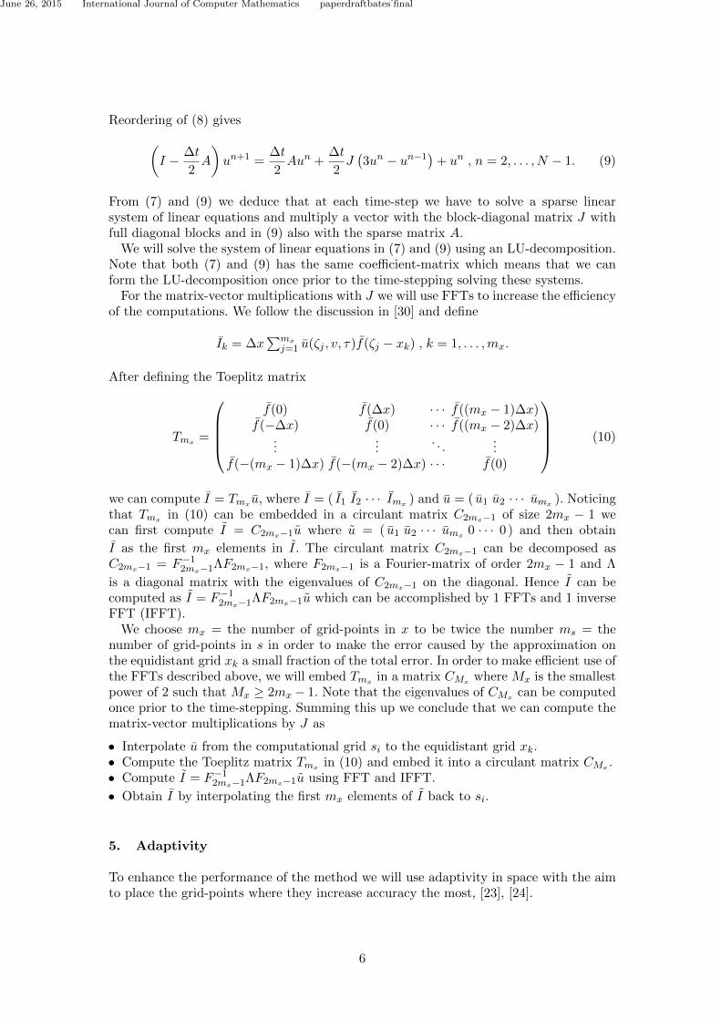
From (7) and (9) we deduce that at each time-step we have to solve a sparse linearsystem of linear equations and multiply a vector with the block-diagonal matrix J withfull diagonal blocks and in (9) also with the sparse matrix A.

We will solve the system of linear equations in (7) and (9) using an LU-decomposition.Note that both (7) and (9) has the same coefficient-matrix which means that we canform the LU-decomposition once prior to the time-stepping solving these systems.

For the matrix-vector multiplications with J we will use FFTs to increase the efficiencyof the computations. We follow the discussion in [30] and define

Ik = ∆x∑mx

j=1 u(ζj , v, τ)f(ζj − xk) , k = 1, . . . ,mx.

After defining the Toeplitz matrix

Tmx=

f(0) f(∆x) · · · f((mx − 1)∆x)

f(−∆x) f(0) · · · f((mx − 2)∆x)...

.... . .

...f(−(mx − 1)∆x) f(−(mx − 2)∆x) · · · f(0)

(10)

we can compute I = Tmxu, where I = ( I1 I2 · · · Imx

) and u = ( u1 u2 · · · umx). Noticing

that Tmxin (10) can be embedded in a circulant matrix C2mx−1 of size 2mx − 1 we

can first compute I = C2mx−1u where u = ( u1 u2 · · · umx0 · · · 0 ) and then obtain

I as the first mx elements in I. The circulant matrix C2mx−1 can be decomposed asC2mx−1 = F−1

2mx−1ΛF2mx−1, where F2mx−1 is a Fourier-matrix of order 2mx − 1 and Λ

is a diagonal matrix with the eigenvalues of C2mx−1 on the diagonal. Hence I can becomputed as I = F−1

2mx−1ΛF2mx−1u which can be accomplished by 1 FFTs and 1 inverseFFT (IFFT).

We choose mx = the number of grid-points in x to be twice the number ms = thenumber of grid-points in s in order to make the error caused by the approximation onthe equidistant grid xk a small fraction of the total error. In order to make efficient use ofthe FFTs described above, we will embed Tmx

in a matrix CMxwhere Mx is the smallest

power of 2 such that Mx ≥ 2mx − 1. Note that the eigenvalues of CMxcan be computed

once prior to the time-stepping. Summing this up we conclude that we can compute thematrix-vector multiplications by J as

• Interpolate u from the computational grid si to the equidistant grid xk.• Compute the Toeplitz matrix Tmx

in (10) and embed it into a circulant matrix CMx.

• Compute I = F−12mx−1ΛF2mx−1u using FFT and IFFT.

• Obtain I by interpolating the first mx elements of I back to si.

5. Adaptivity

To enhance the performance of the method we will use adaptivity in space with the aimto place the grid-points where they increase accuracy the most, [23], [24].

6


We start by considering a PIDE ∂u∂τ + Lu = 0 in one spatial dimension x that we

discretize with a second-order method such that for a computed solution uh ∈ C2 itholds

uh = u+ h2c(x) (11)

after neglecting high-order terms and hence u2h = u+ (2h)2c(x). Using the second-orderaccuracy also in the local discretization error in space ϕh we get

ϕh = h2η(x). (12)

From the definition of the local truncation error ϕh = Lhu− Lu and (11) we get

ϕh = Lhuh − Lu− h2Lhc(x) (13)

and

ϕ2h = L2huh − Lu− h2L2hc(x), (14)

where the term L2huh is defined as the operator L2h acting on every second element inuh. Subtracting (13) from (14) and defining δh = Lhuh and δ2h = L2huh gives

ϕ2h − ϕh = δ2h − δh − h2(L2h − Lh)c(x) = δ2h − δh +O(h4).

Now using (12) and omitting high-order terms we get

η(x) ≈ δ2h − δh3h2

, ϕ(x) =δ2h − δh

3, (15)

i.e. we can estimate η(x) by computing a solution uh using the spatial discretization hand employ (15). If we require |ϕh| = |h2η(x)| < ε for some tolerance ε we can obtainthis by computing a solution using the new spatial discretization h(x) defined by

h(x) = h

√ε

|ϕh(x)|.

To prevent us from using too large spatial steps, we introduce a small parameter d anddefine

h(x) = h

√ε

|ϕh(x)|+ ε · d. (16)

We will use extrapolation of ϕh in two grid-points at the boundaries s = smin, s = smax

and v = vmax to remove the effects caused by the boundary conditions used. To ensurea smooth ϕh we perform some smoothing iterations according to

ϕh(xk) = (ϕh(xk−1) + 2ϕh(xk) + ϕh(xk+1)) /4.

For the PIDE in (2) we get that the local discretization error in space ϕhs,hvcan

be approximated by ϕhs,hv= h2

sηs(s, v) + h2vηv(s, v) + O(h3

s) + O(h3v) if we neglect the

7


influence from the mixed derivatives. Now, proceeding as in the one-dimensional case wecan estimate ϕhs

(s, v) by computing with hs and h2s and similarly for ϕhv(s, v). Then

we compute

ϕhs(s) = maxv |ϕhs

(s, v)|,ϕhv

(v) = maxs |ϕhv(s, v)|.

From |ϕhs(s)| < εs and |ϕhv

(v)| < εv we can compute new one-dimensional grids hs(s)and hv(v) and form a tensor-product grid from these.

Since (2) is time-dependent the local discretization error ϕh will vary in time. We willuse the solution uh at three different time-levels T/3, 2T/3 and T and use max |ϕh| overthese time-steps when we compute the new computational grids.

We end up this section by summarizing the algorithm for adaptivity as follows:

(1) Compute a solution using a coarse spatial grid (mcs,m

cv) and a coarse temporal dis-

cretization with N c time-steps.(2) Estimate the local truncation error on this grid and compute a new spatial grid

(mfs ,m

fv ) using (16) for some given ε.

(3) Compute a new solution using the new spatial grid (mfs ,m

fv ) and Nf time-steps.

The values of mcs, m

cv, N

c, ε, and Nf that we have used can be found in Table 2.For American options the second derivative of the solution over the free boundary sf

is discontinuous. Hence uh ∈ C2 does not hold locally there and we will remove pointsin this region in our estimates of η and ϕ.

Note that the FFTs described in Section 4 are always performed in an equidistant gridin x no matter what the grid looks like in s. This means that for the integral part we willnot really make use of the adaptive grid. However, this will not degrade the performanceof our method as long as the grid xk is fine enough which will be demonstrated in Section7.

6. Operator splitting method

In this section we will describe how we solve the LCP (4). We will use the operatorsplitting method described in [12], [15], [30], for example. For the IMEX-Euler method(6) the operator splitting method is defined by

(I − ∆t

2A

)un+1/2 =

∆t

2Jun +

∆t

2λn , n = 0, 1

2 , 1,32 . (17)

1

∆t

(un+1 − un+1

)− 1

2

(λn+1 − λn

)= 0,

(λn+1

)T (un+1 − Φ

)= 0, un+1 ≥ Φ and λn+1 ≥ 0.

(18)

8


Similarly for the IMEX-CNAB method (8) we have(I − ∆t

2A

)un+1 =

(I +

∆t

2A

)un +

∆t

2J(3un − un−1

)+ ∆tλn , n = 2, . . . ,M − 1,

(19)

1

∆t

(un+1 − un+1

)−(λn+1 − λn

)= 0,

(λn+1

)T (un+1 − Φ

)= 0, un+1 ≥ Φ and λn+1 ≥ 0.

(20)

Hence, we first solve for un+1 using (17) and (19) and then update for un+1 using (18)and (20), respectively.

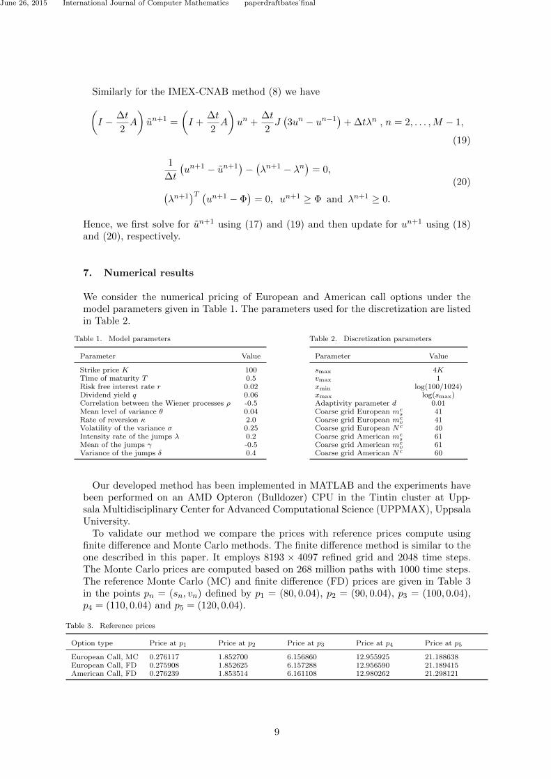
7. Numerical results

We consider the numerical pricing of European and American call options under themodel parameters given in Table 1. The parameters used for the discretization are listedin Table 2.

Table 1. Model parameters

Parameter Value

Strike price K 100Time of maturity T 0.5Risk free interest rate r 0.02Dividend yield q 0.06Correlation between the Wiener processes ρ -0.5Mean level of variance θ 0.04Rate of reversion κ 2.0Volatility of the variance σ 0.25Intensity rate of the jumps λ 0.2Mean of the jumps γ -0.5Variance of the jumps δ 0.4

Table 2. Discretization parameters

Parameter Value

smax 4Kvmax 1xmin log(100/1024)xmax log(smax)Adaptivity parameter d 0.01Coarse grid European mc

s 41Coarse grid European mc

v 41Coarse grid European Nc 40Coarse grid American mc

s 61Coarse grid American mc

v 61Coarse grid American Nc 60

Our developed method has been implemented in MATLAB and the experiments havebeen performed on an AMD Opteron (Bulldozer) CPU in the Tintin cluster at Upp-sala Multidisciplinary Center for Advanced Computational Science (UPPMAX), UppsalaUniversity.

To validate our method we compare the prices with reference prices compute usingfinite difference and Monte Carlo methods. The finite difference method is similar to theone described in this paper. It employs 8193 × 4097 refined grid and 2048 time steps.The Monte Carlo prices are computed based on 268 million paths with 1000 time steps.The reference Monte Carlo (MC) and finite difference (FD) prices are given in Table 3in the points pn = (sn, vn) defined by p1 = (80, 0.04), p2 = (90, 0.04), p3 = (100, 0.04),p4 = (110, 0.04) and p5 = (120, 0.04).

Table 3. Reference prices

Option type Price at p1 Price at p2 Price at p3 Price at p4 Price at p5

European Call, MC 0.276117 1.852700 6.156860 12.955925 21.188638European Call, FD 0.275908 1.852625 6.157288 12.956590 21.189415American Call, FD 0.276239 1.853514 6.161108 12.980262 21.298121

9


For the equidistant method we will use the grids defined in Table 4.

Table 4. Computational grids for equidistant method

Grid # grid-points in s, ms # grid-points in v, mv # time-steps, N

1 34 16 162 64 32 323 130 64 644 258 128 1285 514 256 256

For the adaptive method we will use two different strategies. With Parameter settingI we will adjust εs and εv such that the resulting number of grid-points in the adaptivegrid is the same as in Table 4. The required εs and εv can be found in Table 5. WithParameter setting II we will use εs = εv defined in Table 6.

Table 5. Tolerances and grid sizes for Parameter

setting I

European call option

Grid εs εv mfs mf

v Nf

1I 3.60e-1 1.30e-1 34 16 162I 9.00e-2 2.50e-2 66 32 323I 2.25e-2 5.50e-3 130 64 644I 5.65e-3 1.34e-3 258 128 1285I 1.42e-4 3.27e-4 514 256 256

American call option

Grid εs εv mfs mf

v Nf

1I 4.50e-1 2.50e-1 34 16 162I 1.13e-1 4.30e-2 66 32 323I 2.05e-2 9.50e-3 130 64 644I 7.15e-3 2.30e-3 258 128 1285I 1.79e-3 5.70e-4 514 256 256

Table 6. Tolerances and grid sizes for

Parameter setting II

European call option

Grid εs = εv mfs mf

v Nf

1II 3.60e-1 34 11 162II 9.00e-2 66 18 323II 2.25e-2 130 33 644II 5.65e-3 258 64 1285II 1.42e-4 514 124 256

American call option

Grid εs = εv mfs mf

v Nf

1II 4.50e-1 34 13 162II 1.13e-1 66 21 323II 2.05e-2 130 38 644II 7.15e-3 258 74 1285II 1.79e-3 514 145 256

In Figure 1 we display the computational grids 1I and 1II for the European call optionrespectively.

S

0 100 200 300 400

V

0

0.2

0.4

0.6

0.8

1

S

0 100 200 300 400

V

0

0.2

0.4

0.6

0.8

1

Figure 1. Computational grids 1I (left) and 1II (right).

10


Table 7. European call option

Equidistant grid

Grid Value at p1 Value at p2 Value at p3 Value at p4 Value at p5

1 1.009591 2.256089 6.133288 13.147451 21.4187952 0.321351 1.832901 6.110899 12.964181 21.1990793 0.288398 1.848922 6.146920 12.954746 21.1912824 0.279098 1.851941 6.154781 12.955890 21.1896025 0.276716 1.852481 6.156602 12.956333 21.189251

Adaptive grid, Parameter setting I


1I 0.372584 1.928847 6.126786 12.962764 21.2178822I 0.287465 1.820170 6.096471 12.923203 21.1782423I 0.282472 1.854420 6.153026 12.955278 21.1902614I 0.277213 1.852106 6.155264 12.955607 21.1891215I 0.276306 1.852689 6.156970 12.956404 21.189210

Adaptive grid, Parameter setting II


1II 0.386846 1.922644 6.080406 12.977948 21.2395662II 0.292318 1.806235 6.105908 12.931003 21.1767253II 0.283437 1.851852 6.154529 12.955998 21.1901874II 0.277414 1.851720 6.155369 12.955788 21.1891365II 0.276360 1.852589 6.156992 12.956455 21.189214

Table 8. American call option

Equidistant grid


1 1.079182 2.294828 6.136774 13.181413 21.5283242 0.324001 1.832550 6.108420 12.984336 21.3037393 0.289376 1.849453 6.149199 12.977637 21.2994064 0.279598 1.852736 6.158231 12.979404 21.2983145 0.277090 1.853348 6.160339 12.980003 21.298094

Adaptive grid, Parameter setting I


1I 1.998162 2.915485 6.621065 13.311913 21.5210472I 0.303324 1.854678 6.128726 12.966343 21.2982263I 0.284322 1.856819 6.157372 12.979790 21.2997934I 0.277328 1.851382 6.156941 12.977977 21.2973605I 0.276565 1.853128 6.160219 12.979758 21.297917

Adaptive grid, Parameter setting II


1II 2.114465 2.989597 6.631520 13.356493 21.5404912II 0.305768 1.848060 6.130321 12.970583 21.2973243II 0.284911 1.855239 6.158241 12.980255 21.2996794II 0.277467 1.851111 6.157018 12.978109 21.2973525II 0.276601 1.853060 6.160236 12.979793 21.297915

In Tables 7 and 8 we present the computed solutions using the grids defined in Table 4–6. From the tables we see that the computed option prices converge towards the referenceprices in Table 3 as the spatial grid is refined.

Next we will perform numerical experiments to verify the efficiency of the adaptivemethod. In Table 9–12 we display the error for both equidistant grids and the adaptivegrids defined in Section 5. A comparison with precomputed non-uniform grids would ofcourse also be of interest. However, it is not clear how such a grid should be constructed in

11


the general case and we see the adaptive method presented in this paper as a simple andefficient way to create such grids. In [36] a comparison of e.g. finite difference methodson equidistant grids, precomputed non-uniform grids and adaptive grids is presented fora set of benchmarking problems.

We compare the computed solutions with a computed reference solution on a fineadaptive grid with 1026 grid-points in s and 512 points in v. The error is measured inthe domain

ΩK = (s, v)|K2 ≤ s ≤3K2 , 0 ≤ v ≤ 0.16,

which we consider to be the domain where we are most interested in having an accuratesolution. Both a numerical approximation of the L2-norm of the error and the max-normof the error is displayed. The quotients Qi presented are defined as

Qi =Error in grid (i− 1)

Error in grid i.

We also show the average quotient Q =(∑5

i=2Qi

)/4.

Table 9. Convergence in L2-norm for European call option in ΩK .

Grid # time-steps Equidistant Q Adaptive I Q Adaptive II Q

1 / 1I / 1II 16 2.19e-0 - 1.87e-1 - 2.57e-1 -2 / 2I / 2II 32 1.77e-1 12.4 1.04e-1 1.80 1.55e-1 1.703 / 3I / 3II 64 4.78e-2 3.71 1.05e-2 9.90 2.54e-2 6.104 / 4I / 4II 128 9.41e-3 5.08 2.97e-3 3.54 5.00e-3 5.045 / 5I / 5II 256 1.61e-3 5.84 4.46e-4 6.65 7.76e-4 6.55

Q 6.76 5.47 4.85

Table 10. Convergence in max-norm for European call option in ΩK .



Q 4.25 4.92 3.88

Table 11. Convergence in L2-norm for American call option in ΩK .



Q 6.96 24.6 19.4

From Tables 9–12 we see that we obtain in almost all cases at least the expectedsecond-order convergence for both the equidistant and adaptive methods. We also see

12


Table 12. Convergence in max-norm for American call option in ΩK .



Q 4.29 10.9 7.99

that for a given number of grid-points, the error for the adaptive method is most oftensmaller than the error for the equidistant one. Note however, that for the finest adaptivegrids, the spatial discretization parameter is quite close to the one from the referencegrid. Hence, this error estimate is not as accurate as for the coarser grids.

Error

10-3

10-2

10-1

100

Co

mp

uta

tio

na

l tim

e

10-2

100

102

104

European option, L2-norm

Equidistant

Adaptive I

Adaptive II

Error

10-3

10-2

10-1

100

Co

mp

uta

tio

na

l tim

e

10-2

100

102

104

European option, max-norm

Equidistant

Adaptive I

Adaptive II

Error

10-3

10-2

10-1

100

Co

mp

uta

tio

na

l tim

e

10-2

100

102

104

American option, L2-norm

Equidistant

Adaptive I

Adaptive II

Error

10-3

10-2

10-1

100

Co

mp

uta

tio

na

l tim

e

10-2

100

102

104

American option, max-norm

Equidistant

Adaptive I

Adaptive II

Figure 2. Computational time as a function of error for European option, L2-norm (top left), European option,

max-norm (top right), American option, L2-norm (bottom left) and American option, max-norm (bottom right).

In Figure 2 we display the computational time as a function of the error in Tables 7and 8. From this figure it is clear that for errors less than approximately 10−1 in theL2-norm and less than approximately 3 · 10−1 in the max-norm, it is beneficial to usethe adaptive methods. For errors less than approximately 5 · 10−2–10 · 10−2, the gainin computational time by using the adaptive methods is up to 20 times, depending onwhich option, parameter-setting and norm we are considering.

For the larger errors (> 10−1), the computation of the solution on the coarse grid toestimate the local truncation error (step (1) in the adaptive method) takes relativelytoo much time of the whole adaptive algorithm. Thus, the adaptive methods are notcompetitive when we are satisfied with relatively large errors in the final solution.

We see that the gain by using the adaptive technique is larger in the max-norm whichmakes sense since the refinement of the grid is localized in the most difficult areas whereit is likely the maximal error occurs.

13


8. Conclusions

In this paper we have developed an adaptive finite difference method to price optionsunder the Bates model. This model gives rise to a parabolic PIDE that we discretize usingan IMEX-scheme in time. The integrals that occur on the explicit side are computed usingFFTs, while the spatial derivatives are discretized using second-order finite differences.For the LCPs occuring in the pricing of American options we employ an operator splittingmethod.

By estimating the local truncation error on a coarse equidistant grid, a new adaptivegrid is computed such that an estimate of the final local truncation error is below aprescribed tolerance level. We have tried two different strategies in the computation ofthe adaptive grids. For both strategies it holds that if we want reasonably sized errorsin the final solution, it is always beneficial to use the adaptive method compared toequidistant grids. To reach a given fairly high accuracy level, the computational timecan be reduced up to 20 times.

Acknowledgments

The work in this paper builds on the sequence of Master theses/project reports [32], [31],[37] and [38]. The authors are thankful for the early contributions of these students.

The computations were performed on resources provided by the Swedish NationalInfrastructure for Computing (SNIC) through Uppsala Multidisciplinary Center for Ad-vanced Computational Science (UPPMAX) under Projects snic2014-3-24 and snic2015-6-77.

The first author was financed by the Swedish Research Council under contract number621-2007-6388.

We thank the referees for their suggestions and comments.

References

[1] Y. Achdou and O. Pironneau, Computational methods for option pricing, Frontiers in Applied Math-ematics, Vol. 30, SIAM, Philadelphia, PA, 2005.

[2] A. Almendral and C.W. Oosterlee, Numerical valuation of options with jumps in the underlying,Appl. Numer. Math. 53 (2005), pp. 1–18.

[3] L. Andersen and J. Andreasen, Jump-diffusion processes: Volatility smile fitting and numerical meth-ods for option pricing, Rev. Deriv. Res. 4 (2000), pp. 231–262.

[4] D.S. Bates, Jumps and stochastic volatility: Exchange rate processes implicit Deutsche mark options,Review Financial Stud. 9 (1996), pp. 69–107.

[5] F. Black and M. Scholes, The pricing of options and corporate liabilities, J. Polit. Econ. 81 (1973),pp. 637–654.

[6] C. Chiarella, B. Kang, G.H. Meyer, and A. Ziogas, The evaluation of American option prices understochastic volatility and jump-diffusion dynamics using the method of lines, Int. J. Theor. Appl.Finance 12 (2009), pp. 393–425.

[7] N. Clarke and K. Parrott, Multigrid for American option pricing with stochastic volatility, Appl.Math. Finance 6 (1999), pp. 177–195.

[8] R. Cont and E. Voltchkova, A finite difference scheme for option pricing in jump diffusion andexponential Levy models, SIAM Numer. Anal. 43 (2005), pp. 1596–1626.

[9] Y. d’Halluin, P.A. Forsyth, and G. Labahn, A penalty method for American options with jumpdiffusion processes, Numer. Math. 97 (2004), pp. 321–352.

[10] Y. d’Halluin, P.A. Forsyth, and K.R. Vetzal, Robust numerical methods for contingent claims underjump diffusion processes, IMA J. Numer. Anal. 25 (2005), pp. 87–112.

14


[11] S. Heston, A closed-form solution for options with stochastic volatility with applications to bond andcurrency options, Rev. Financial Stud. 6 (1993), pp. 327–343.

[12] S. Ikonen and J. Toivanen, Operator splitting methods for American option pricing, Appl. Math.Lett. 17 (2004), pp. 809–814.

[13] S. Ikonen and J. Toivanen, Componentwise splitting methods for pricing American options understochastic volatility, Int. J. Theor. Appl. Finance 10 (2007), pp. 331–361.

[14] S. Ikonen and J. Toivanen, Efficient numerical methods for pricing American options under stochas-tic volatility, Numer. Methods Partial Differential Equations 24 (2008), pp. 104–126.

[15] S. Ikonen and J. Toivanen, Operator splitting methods for pricing American options under stochasticvolatility, Numer. Math. 113 (2009), pp. 299–324.

[16] K.J. In ’t Hout and S. Foulon, ADI finite difference schemes for option pricing in the Heston modelwith correlation, Int. J. Numer. Anal. Model. 7 (2010), pp. 303–320.

[17] Y. Kwon and Y. Lee, A second-order finite difference method for option pricing under jump-diffusionmodels, SIAM J. Numer. Anal. 49 (2011), pp. 2598–2617.

[18] Y. Kwon and Y. Lee, A second-order tridiagonal method for American options under jump-diffusionmodels, SIAM J. Sci. Comput. 33 (2011), pp. 1860–1872.

[19] P. Lotstedt, J. Persson, L. von Sydow, and J. Tysk, Space-time adaptive finite difference method forEuropean multi-asset options, Comput. Math. Appl. 53 (2007), pp. 1159–1180.

[20] R.C. Merton, Theory of rational option pricing, Bell J. Econom. Man. Sci. 4 (1973), pp. 141–183.[21] E. Miglio and C. Sgarra, A finite element discretization method for option pricing with the Bates

model, S~eMA J. (2011), pp. 23–40.[22] C.W. Oosterlee, On multigrid for linear complementarity problems with application to American-

style options, Electron. Trans. Numer. Anal. 15 (2003), pp. 165–185.[23] J. Persson and L. von Sydow, Pricing European multi-asset options using a space-time adaptive

FD-method, Comput. Vis. Sci. 10 (2007), pp. 173–183.[24] J. Persson and L. von Sydow, Pricing American options using a space-time adaptive finite difference

method, Math. Comput. Simulation 80 (2010), pp. 1922–1935.[25] A. Ramage and L. von Sydow, A multigrid preconditioner for an adaptive Black-Scholes solver, BIT

51 (2011), pp. 217–233.[26] C. Reisinger and G. Wittum, On multigrid for anisotropic equations and variational inequalities:

Pricing multi-dimensional European and American options, Comput. Vis. Sci. 7 (2004), pp. 189–197.[27] S. Salmi and J. Toivanen, An iterative method for pricing American options under jump-diffusion

models, Appl. Numer. Math. 61 (2011), pp. 821–831.[28] S. Salmi and J. Toivanen, IMEX schemes for pricing options under jump-diffusion models, Appl.

Numer. Math. 84 (2014), pp. 33–45.[29] S. Salmi, J. Toivanen, and L. von Sydow, Iterative methods for pricing American options under the

Bates model, in Proceedings of 2013 International Conference on Computational Science, ProcediaComputer Science Series, Vol. 18, Elsevier, 2013, pp. 1136–1144.

[30] S. Salmi, J. Toivanen, and L. von Sydow, An IMEX-scheme for pricing options under stochasticvolatility models with jumps, SIAM J. Sci. Comput. 36 (2014), pp. B817–B834.

[31] A. Sjoberg, Adaptive finite differences to price European options under the Bates model, Master’sthesis, Department of Information Technology, Uppsala University, 2013, iT Report 13 063.

[32] R. Skogberg and J. Markhed, Pricing European options using stochastic volatility and integral jumpterm (2009).

[33] D. Tavella and C. Randall, Pricing financial instruments: The finite difference method, John Wiley& Sons, Chichester, 2000.

[34] J. Toivanen, A componentwise splitting method for pricing American options under the Batesmodel, in Applied and numerical partial differential equations, Comput. Methods Appl. Sci., Vol. 15,Springer, New York, 2010, pp. 213–227.

[35] J. Toivanen and C.W. Oosterlee, A projected algebraic multigrid method for linear complementarityproblems, Numer. Math. Theory Methods Appl. 5 (2012), pp. 85–98.

[36] von Sydow L., H. L.J., L. E., L. E., M. S., P. J., S. V., S. Y., S. S., T. J., W. J., W. M., L. J., L.J., O. C.W., R. M.J., T. A., and Z. Y., BENCHOP–the BENCHmarking project in Option PricingAccepted for publication.

[37] A. Westlund, An IMEX-method for pricing options under Bates model using adaptive finite differ-ences (2014).

[38] C. Zhang, Fast Fourier transforms in IMEX-schemes to price options under Bates model, Master’sthesis, Uppsala University, 2014.

[39] R. Zvan, P.A. Forsyth, and K.R. Vetzal, Penalty methods for American options with stochastic

15


volatility, J. Comput. Appl. Math. 91 (1998), pp. 199–218.[40] R. Zvan, P.A. Forsyth, and K.R. Vetzal, Robust numerical methods for PDE models of Asian options,

J. Comput. Finance 1 (1998), pp. 39–78.

16

Documents

Postpr int - DiVA portaluu.diva-portal.org/smash/get/diva2:852147/FULLTEXT01.pdf · Postpr int This is the accepted version of a paper published in International Journal of Computer