Position Stability For Phase Control Of The Preisach Hysteresis

Position Stability For Phase Control Of The Preisach Hysteresis Model

Juan Manuel Cruz-Hernandez∗and Vincent Hayward†

Abstract. Many systems with hysteresis are adequately represented by the Preisach model.Hysteresis in these systems can be very effectively reduced using the “phaser”, an ideal frequencydomain operator, in a feedback connection. The position stability of this type of control has notyet been established in spite of the experimental evidence that the resulting systems are stable.This paper shows the dissipativity for the relay operator, for the Preisach model, and then for thelead approximation to the phaser. We then give a proof of stability for the feedback connection ofthis phaser approximation with systems represented by the Preisach model of hysteresis.

1 Introduction

Actuators used in robotics and other applications often exhibit hysteresis which is detrimental toperformance. For example, it is well known that most hydraulic actuators have significant hysteresisarising from the valve magnetic activation and friction in the seals [1]. Most strain-based actuatorsalso have hysteresis, specifically actuators based on materials like piezoceramics, shape memoryalloys, or magnetostrictive materials [9, 16].

To improve tracking precision, reduce steady-state error, and achieve other performance objec-tives, feedback controllers have been proposed (for recent contributions among others see [2, 3, 4,17]), however little has been said about their stability. Gorbet et al. have shown the stability ofvelocity feedback control applied to the Preisach hysteresis model (Fig. 1a) [11], or in a similarconfiguration as in [10], but nothing was said about position control (Fig. 1b).

aH1

ddt__ Γ

u2

u1

y2 e2

e1 y1 bH1

Γu2

u1

y2 e2

e1 y1

H2 =

Figure 1: Control Systems Setup. a) Velocity configuration as in [11]. b) Position configuration asdiscussed here. H1 represents the controllers, H2 represents the plant and Γ the Preisach model.

In this paper, we investigate the dissipativity of the Preisach model, in such a manner thatstability of a feedback connection with a given controller can be tested using dissipativity theory [12].The phaser is an ideal operator in the frequency domain which shifts the phase of a signal by a givenamount but leaves the magnitude unchanged and was shown experimentally to be very effective atreducing hysteresis present in strain-based actuators [5]. An ideal phaser cannot be implemented

∗Immersion Canada Inc., Montreal, Qc, H2X 2T7, Canada, [email protected].†Center for Intelligent Machines, McGill University, Montreal, Qc, H3A 2A7, Canada, [email protected].

1

Transactions of the CSME, Vol. 29, No. 2, pp. 129-142, 2005.

but can be approximated by a causal filter. One attractive possibility is a multiple lead networkwhich is easy to design given performance specifications. Stability is investigated for this case, butother choices could be used as well as long as they satisfy the conditions stated in Section 3.

The Preisach model is a popular model for rate-independent hysteresis. It is constructed fromthe combination of an infinite number of elementary relays that serve as “atoms of hysteresis” [14].All the relays receive the same input and there is one relay for each possible pair (α, β) of ‘on’ and‘off’ switching thresholds. The outputs of all the relays are combined using a weighted sum over allthe values of α and β. The weighting function entirely specifies a particular hysteresis. This modelis briefly reviewed in the next section.

Dissipativity analysis begins with that of a single relay operator. This allows us to show thedissipativity of the Preisach model. We introduce a new representation of the relay operator, interms of the feedback connection of two singular nonlinearities. With this, dissipativity can beobtained and extended to the dissipativity of the Preisach model. The lead approximation to thephaser can be shown to be dissipative too. In Section 4, we use a theorem by Hill and Moylan forthe single-input single-output case to show that the feedback connection of the Preisach model andthe approximation to the phaser is stable [12].

2 The Preisach model

The Preisach model results from the combination of relay operators such as the one shown inFig. 2a.

a

αβ u

γβα

b

−α

−β

u γβα

1

−1

1−1

u1

y2 u2

y1

Figure 2: a) Relay operator. b) Equivalent representation of a relay using a feedback connection.

The real-valued weighting function µα,β, the Preisach function, with support H in α ≥ β,describes the relative contribution of an infinite collection of relays sharing the same input. Thehysteresis output using the Preisach model is written:

y(t) = Γ[u(t)] =∫∫

Hµα,β γαβ [u(t)] dα dβ (1)

In α, β coordinates, each point of the half plane α ≥ β is identified with only one particular γ-operator whose on and off switching values are respectively found at the α and β coordinates ofthe point (γαβ : R 7→ {−1, 1}). The weighted output of a particular relay will be identified byyαβ(t) = µαβ γαβ [u(t)]. In practice, the support for µαβ is finite [11, 14]. This means µαβ = 0outside the triangle α = u2, β = u1, α = β. This can be thought of as restricting H to a triangle,as in Fig. 3b.

2


a

u2

H α β=

α

βusatu1

b

u2

H

α

βu1

Figure 3: Limiting triangle for the Preisach model.

In systems which have nonzero slope outside the loop, such as some magnetic materials, de-generated relays must be added along the diagonal α = β in order to complete the model. Evenin this case, physical limits such as control signal saturation, say at usat, allow H to be effectivelybounded (Figure 3a). The gray area indicates the contributing relays, and the finite support H forµ is delimited by the dotted line.

For physical hysteresis (e.g. shape memory alloys, piezoceramics actuators, magnetostrictiveactuators), it is reasonable to assume that H is bounded in α ≥ β. It is also clear that µ must be:

• non-negative, otherwise an increase in input could cause a decrease in output, and

• finite, since the major hysteresis loop is closed in the input-output plane.

Assumption 2.1 (Finite Support [11])It will be assumed that the Preisach weighting function µ is finite, non-negative and has finitesupport: H = {(α, β)|α ≤ u2, β ≥ u1, α ≥ β}, with u2 > u1.

2.1 Background

Here, we follow the presentation of Subsection 2.2 in [11]. The mathematical background can befound for example in [8], however the notation used in [11] is employed for convenience.

L2(R) is the set of all functions f : R 7→ R such that∫∞−∞ f(t)2dt < ∞. It is known that L2(R)

is a normed vector space with the L2-norm defined by ‖f‖ = (∫∞−∞f(t)2dt)1/2. For any T ≥ 0,

consider the subset L2[0, T ] of L2(R) defined by L2[0, T ] = {f : R 7→ R| f(t) = 0 ∀ t /∈ [0, T ]}.The subset L2[0, T ] with ‖f‖ of L2(R) is also a normed vector space. For every f ∈ L2[0, T ],‖f‖ = (

∫∞−∞f(t)2dt)1/2 = (

∫ T0 f(t)2dt)1/2. Consequently ‖f‖T = (

∫ T0 f(t)2dt)1/2 is a norm for

L2[0, T ]. Define the truncation of f ∈ L2(R), for any T ≥ 0, to be fT (t) = f(t) for 0 ≤ t ≤ Tand fT (t) = 0 for t > T . The extended space L2e is composed of functions fT (t) for which∫∞0 fT (t)2dt < ∞. Given two functions f and g in L2(R), the inner product of these two functions

is defined as 〈f, g〉 =∫∞−∞f(t)g(t) dt. For f and g in L2[0, T ], 〈f, g〉T = 〈xT , yT 〉 =

∫∞−∞f(t)g(t) dt =∫ T

0 f(t)g(t) dt.Hysteresis is a nonlinearity with memory which implies that the output may be affected by

the entire history of past inputs. The same input applied to a hysteretic system at t0 > 0 mayyield different outputs, depending on the input history over [0, t0]. This makes it difficult to definea “relaxed state”, as is typically done in passivity analysis. This is because the natural physicalinterpretation of relaxation: setting the input to zero and letting t → ∞, may lead to differentequilibria at any point along the axis where the input is zero. The relaxed state for such a system

3


is not unique, and may correspond to an entire set of outputs. Relations are introduced in orderto deal with the multi-valued nature of the output, and to avoid having to define a unique relaxedstate.

Definition 2.1 (Relation [11])A relation H on L2[0, T ] defines a set of ordered pairs (x, y) ∈ L2[0, T ]×L2[0, T ]. The domain andrange of H can be defined as follows:

Do(H) = {x ∈ L2[0, T ] | ∃y ∈ L2[0, T ] s.t. y = Hx},Ra(H) = {y ∈ L2[0, T ] | ∃x ∈ L2[0, T ] s.t. y = Hx},

A relation may be multi-valued, meaning that for any x ∈ Do(H), there may be several y ∈L2[0, T ] such that y = Hx, and this multi-valued property makes the relations useful in describinghysteretic systems. When something is said to hold (or is required to hold) for Hx, withoutqualification, it will be understood that it holds (or is required to hold) for all possible outputscorresponding to the input x. It is also important to note that H need not be defined on the wholeof L2[0, T ].

Definition 2.2 (Sobolev Space)The Sobolev Space W 2

1 [0, T ] is the space of functions u ∈ L2[0, T ] for which the Sobolev norm isfinite:

‖u‖W 21

=

√∫ T

0(u2 + u2)dt. (2)

Clearly, if u ∈ W 21 [0, T ], then u ∈ L2[0, T ].

The following definitions are needed for the next theorem [11]. Define Rα and Rβ, horizontaland vertical strips in H, and the function k as follows:

Rα(λ, ξ) , {(α, β) ∈ H|λ ≤ α ≤ λ + ξ}Rβ(λ, ξ) , {(α, β) ∈ H|λ ≤ β ≤ λ + ξ}

k(ξ) , supλ∈R,R∈{Rα,Rβ}

∫∫R

µαβ dα dβ

Theorem 2.1 (in [11])Suppose µ is finite and non-negative on H. The Preisach operator maps W2

1[0, T ] into itself if andonly if there exists C > 0 such that k(ξ) ≤ Cξ for all ξ > 0.

The conditions of the above theorem hold if the support H is finite, and µ is finite and non-negative.

Corollary 2.1 (Claim 2.1 in [11])If H is finite and 0 ≤ µαβ < ∞ for all (α, β) ∈ H, then there exists C > 0 such that k(ξ) ≤ Cξ forall ξ > 0.

Given the above Claim and Assumption 2.1, Theorem 2.1 applies and Γ : W21[0, T ] 7→ W2

1[0, T ].

4


2.2 The Phaser Controller [5]

Assume that the input to a hysteretic system varies periodically between two values. The Preisachmodel predicts that a loop is produced in the input-output graph. It is then possible to speak ofphase shift between input and output. The loop and the output will have the same period as theinput and the effect can be viewed as phase lag between input and output. Moreover, the phaselag angle φ is constant if rate independence holds [6]. Consider the following:

Definition 2.3 (in [5])A Phaser Lpa is an operator that shifts a periodic input signal by a constant angle, and has unitygain.

The phaser operator can be seen as the counterpart of the proportional controller for whichthe phase is zero but the magnitude is adjusted according to design specifications. The phaserkeeps the magnitude constant but applies a given phase shift at all frequencies according to designspecifications.

The effect of the phaser used in a feedback loop can be intuitively appreciated by consideringa Fourier series expansion of the input signal. Periodic signals can be decomposed into a combina-tion of sinusoidal signals with frequencies 1

T , 2T , . . . , k

T where 1T is the fundamental frequency. All

components of a signal distorted by rate independent hysteresis are shifted the same way and allare corrected the same way. Since it is only an approximation, the correction cannot be perfect, soan error term e (distortion) is formed for further correction by feedback. Moreover, when dealingwith nonlinear systems, in some cases, it is possible to only consider the fundamental componentof the output (as in the describing function analysis).

A phaser is an idealization that cannot be implemented because no causal physical system canprovide a constant phase shift over an infinite frequency range. However, a phaser can be approx-imated by causal linear filters. Among other choices, the following transfer function represents aphaser controller approximated by a lead network, with all the factors covering adjacent frequencybands:

Lpa(s) =(

s + pn

s + qn

)(s + pn−1

s + qn−1

). . .

(s + p1

s + q1

), (3)

where the pi and qi are greater than zero for i = 1, . . . , n. This fraction can be rearranged suchthat pi > qi for all i’s. Properly designed, the phase of Lpa(s) will be nearly constant within a widefrequency range. A phaser Lpa(jω) in the complex plane has a Nyquist plot as in Fig. 4 for any n.

Im

Re

Figure 4: Nyquist plot of the linear approximation to the phaser as in Eqn (3).

It is clear that the real part of Lpa(jω) is always positive and different from zero for all ω, andthat it has a well defined lower bound (it is continuously bounded). Also note that ||Lpa(jω)|| is

5


bounded above by 1 for all ω. The product Lpa(jω)Lpa(−jω) is also positive since each factor inEqn (3) will be multiplied by its corresponding complex conjugate, yielding a positive number.

Lpa(jw)Lpa(−jw) =(

jω + pn

jω + qn

)(−jω + pn

−jω + qn

). . .

(jω + p1

jω + q1

)(−jω + p1

−jω + q1

). (4)

Therefore the product will be also bounded by a finite positive number and will be different fromzero. Thus we have

∀ω, A = 2maxω

(Lpa(jω)Lpa(−jω)

Re[Lpa(jω)]

)> 0, B = max

ω

(π

Re[Lpa(jω)]

)> 0 (5)

which we will use in Section 3.3.

3 Dissipativity

Definition 3.1 (Dissipativity, modified from [13])Given a relation G on L2e, with y = Gu, and q, r, s ∈ R, G is said to be (q, r, s)-dissipative iff,

〈y, qy〉T + 〈y, su〉T + 〈u, ru〉T ≥ 0 (6)

for all u ∈ Do(G) and all T ≥ 0.

3.1 Dissipativity of the Relay Operator

Consider one single relay y = yαβ and the scalars q, s, and r. Assume u is in the Sobolev space,i.e. u ∈ W2

1[0, T ], and the Preisach function µαβ is finite, then y = yαβ is also finite. A relayoperator can be replaced by a feedback connection as in Fig. 2b. If m = α−β

2 and b = −α+β2 then,

this system is equivalent to that in Fig. 2a. In both cases y2(t) = α−β2 sgn(u1(t)) − α+β

2 . Also, inFig. 2b, the following holds:

u(t) = u1(t)− y2(t) (7)u1(t)u2(t) = |u1(t)| (8)

y2(t) = m u2(t) + b. (9)

Note also that a weighted relay operator is represented by yαβ = µαβ γαβ . For simplicity takeµαβ = 1 and y = γαβ , then the product u y is:

u(t)y(t) = u(t)γαβ = u1(t)y1(t)− u2(t)y2(t)= u1(t)sgn(u1(t))−m u2

2(t)− b u2(t)= |u1(t)| −m u2

2(t)− b u2(t). (10)

Expressing −m u22(t) − b u2(t) in terms of α and β, with u2

2(t) = 1, u2(t) = ±1, m = α−β2 , and

b = −α+β2 , we get

−m u22(t)− b u2(t) = −m− b u2(t)

={−m− b = −α−β

2 + α+β2 = β for u2 = 1

−m + b = −α−β2 − α+β

2 = −α for u2 = −1(11)

6


Therefore Eqn (10) can be expressed as,

u(t)y(t) ={|u1(t)|+ β for u2 = 1|u1(t)| − α for u2 = −1

(12)

Now, the dissipativity result.

Lemma 3.1 (Dissipativity of a relay operator)Let the real-valued function u(t), and the relation γαβ, (y(t) = γαβ [u(t)]) be in W2

1[0, T ]. Theweighted relay operator is dissipative with respect to:

q = 0, (13)for some r � 1, (14)

and s = min(α,β∈H,∀µαβ)

1max(µαβ |α|, µαβ |β|)

> 0. (15)

That is:

s

∫ T

0u(t)y(t)dt + r

∫ T

0u2(t)dt ≥ 0 (16)

∀t, 0 ≤ t ≤ T , ∀T ≥ 0, and u ∈ Do(γαβ).

Proof: For all T ≥ 0, and all α and β in H, and u ∈ Do(H), the following equality holds,

r

∫ T

0u2(t)dt + s

∫ T

0u(t)y(t)dt =

∫ T

0

(r u2

2(t) + s|u1(t)| − sm u22(t)− s b u2(t)

)dt, (17)

by using Eqn (10). We must prove that the right hand side of Eqn (17) is greater than or equal tozero. Using Eqn (12), it is equivalent to show that

r u22(t) + s|u1(t)| − sm u2

2(t)− s b u2(t) ={

r u2(t) + s|u1(t)|+ s β for u2(t) = 1,r u2(t) + s|u1(t)| − sα for u2(t) = −1.

Consider now both cases independently, choose r > 0 and s > 0, and take into account thatu1(t) = u(t) + y2(t),

u2(t) = 1

For this case u1(t) = u(t)− β, then we have

r u2(t) + s|u1(t)|+ s β = r u2(t) + s |u(t)− β|+ s β. (18)

Consider here the following subcases:

• β ≥ 0: In this case r u2(t) + s |u(t)− β|+ s β ≥ 0 for any value of u(t).

• β < 0: We will make the value of s s.t. s|β| < 1 for all β, and the value of r � 1.Then if

7


I u(t) ≥ 0: Eqn (18) can be expressed as

r u2(t) + s |u(t) + |β| | − s|β| ≥ 0 (19)

I u(t) ≤ −1: Since r � 1 and s|β| < 1, Eqn (18) is greater than zero.I −1 < u(t) < 0: Eqn (18) attains its minimum for u(t) ∈ (−1, 0) and any β.

Because r � 1 and s|β| < 1, Eqn (18) is always positive.

u2(t) = −1

For this case u1(t) = u(t)− α, then we have

r u2(t) + s|u1(t)| − sα = r u2(t) + s |u(t)− α| − sα. (20)

Consider the following subcases and use similar arguments as for u2(t) = 1

• α ≤ 0: r u2(t) + s |u(t)− α| − sα ≥ 0, for any u(t)

• α > 0: Again take s such that s|α| < 1 for all α, and r � 1, then

I u(t) ≤ 0: Eqn (20) is equal to (r u2(t) + s|u(t)− α| − sα) ≥ 0I u(t) ≥ 1 and u(t) ∈ (−1, 0): Similarly, Eqn (20) attains its minimum for u(t) ∈ (0, 1)

and any α. Because r � 1 and s|α| < 1, Eqn (20) is always positive.

The value of s can be:s = min

(α,β∈H)

1max(|α|, |β|)

(21)

which clearly satisfies the conditions stated above, and it is never zero since α and β are finitenumbers. It has been proven that the argument of the integral in the r.h.s. of Eqn (17) is greaterthan or equal to zero for all α and β in H and u ∈ Do(H). Therefore Eqn (17) is always positive:

r

∫ T

0u2(t)dt + s

∫ T

0u(t)y(t)dt =

∫ T

0

(r u2

2(t) + s |u1(t)| − sm u22(t)− s b u2(t)

)dt ≥ 0 (22)

for any T ≥ 0.For a weighted relay operator the result holds, since y is multiplied by an arbitrary µαβ which

is always positive. This will alter the expression in the r.h.s. of Eqn (17) where s will be multipliedby a positive and finite number µαβ . We can take sµαβ |α| < 1 and sµαβ |β| < 1 for all possiblevalues of α and β. Now s can be expressed as:

s = min(α,β∈H,∀µαβ)

1max(µαβ |α|, µαβ |β|)

(23)

This concludes the proof.

8


3.2 Dissipativity of the Preisach Model

The dissipativity of the Preisach model is now derived.

Lemma 3.2 (Dissipativity of the Preisach model)Let the real-valued function u(t), and the relation Γ, (y(t) = Γ[u(t)]) be in W2

1[0, T ]. The Preisachmodel is dissipative with respect to q = 0, r = srelay rrelay

∫∫H µαβ dαdβ > 0 and s = srelay > 0, i.e.

s

∫ T

0u(t)y(t)dt + r

∫ T

0u2(t)dt ≥ 0

for all 0 ≤ t ≤ T , for all T ≥ 0 and u ∈ Do(Γ) and all points in H. srelay and rrelay are the valuesfound in lemma 3.1.

Proof: First evaluate:

s

∫ T

0u(t)y(t)dt = s

∫ T

0u(t)

(∫∫H

yαβ dαdβ

)dt

= s

∫ T

0u(t)

(∫∫H

µαβ γαβ dαdβ

)dt

= s

∫∫H

µαβ

(∫ T

0u(t)γαβ dt

)dαdβ

Using the fact that a relay operator is dissipative for every point in H, and all u ∈ Do(Γ) as inlemma 3.1, yields

srelay

∫ T

0u(t)y(t)dt ≥ srelay

∫∫H

µαβ

(−rrelay

∫ T

0u2(t)dt

)dαdβ

= −∫ T

0u2(t)dt · srelay

∫∫H

µαβ rrelay dαdβ

≥ −r

∫ T

0u2(t)dt (24)

The value r = srelay rrelay

∫∫H µαβ dαdβ is always positive since µαβ is positive and finite. Therefore

the Preisach model is dissipative.

3.3 Dissipativity Of The Lead Approximation Of A Phaser

To prove that the lead approximation to the phaser is dissipative, a proof using Parseval’s theoremsimilar to the proofs of passivity in linear systems is used [8, 18]. We consider that the transferfunction that approximates the ideal phaser is rational with relative degree 0, and causal. Thiscompensates a hysteretic system by providing phase in the feedback that is always smaller then orequal to 90o.

Lemma 3.3 (Modified from [8])The linear system L : W2

1 → W21 defined by

Lu = l ∗ u, where L is causal and u ∈ W21 (25)

is said to be passive iff Re[L(jω)] ≥ 0, ∀ω ∈ R.

9


The lead approximation to the phaser is causal and passive, i.e. strictly stable. We use thisresult to show that the controller is also dissipative.

Lemma 3.4 (Dissipativity of the lead approximation)The lead approximation to the phaser Lpa : W2

1 → W21, causal and strictly stable (passive), is

dissipative with respect to

r < 0q ≤ −α r2 < 0 and

s ≥ −qA− rB, A = 2maxω


Re[Lpa(jω)]

), B = max

ω

(π

Re[Lpa(jω)]

), (26)

i.e. r

∫ T

0u(t)2dt + s

∫ T

0y(t)u(t)dt + q

∫ T

0y(t)2dt ≥ 0

∀t, 0 ≤ t ≤ T , ∀T ≥ 0 and u ∈ W21, r2 being the r found in the dissipativity of the Preisach model.

The value of q is taken to meet the stability conditions of the feedback connection of the Preisachmodel with a dissipative controller as will be shown in the next section. The value of s and r areobtained as follows.

Assume that y(jω)/u(jω) = Lpa(jω), is initially at rest (y ≡ 0). If the input u is zero for allt > T and t < 0, then using the passivity property of the system we have:∫ T

0y(t)u(t)dt =

∫ ∞

−∞y(t)u(t)dt, (27)

=12π

∫ ∞

−∞y(jω)u∗(jω)dω. (28)

The first equality holds because u(t) = 0 for t > T and for t < 0. The second equality comes fromthe Parseval’s theorem, with the superscript * referring to complex conjugation. Since y(jω) =Lpa(jω)u(jω), then ∫ T

0y(t)u(t)dt =

12π

∫ ∞

−∞Lpa(jω)|u(jω)|2dω (29)

Since Lpa is the transfer function of a real system, its coefficients are real and thus Lpa(−jω) =[Lpa(jω)]∗, then ∫ T

0y(t)u(t)dt =

1π

∫ ∞

0Re[Lpa(jω)]|u(jω)|2dω (30)

(This also follows from the fact that the system is passive).Note also that ∫ T

0y(t)2dt =

2π

∫ ∞

0L∗

pa(jω)u∗(jω)Lpa(jω)u(jω)dω, (31)

=2π

∫ ∞

0Lpa(jω)Lpa(−jω)|u(jω)|2dω, (32)

10


which is obtained after using the same arguments (u(t) = 0 for t > T and t < 0 and the Parseval’stheorem).

Expressions (30) and (32) are used to prove the dissipativity of the lead approximation to thephaser. It has to be shown that,

r

∫ T

0u(t)2dt + s

∫ T

0y(t)u(t)dt− q

∫ T

0y(t)2dt

= r

∫ ∞

−∞|u(jω)|2dω + s

1π

∫ ∞

−∞Re[Lpa(jω)]|u(jω)|2dω + q

2π

∫ ∞

−∞Lpa(jω)Lpa(−jω)|u(jω)|2dω

=∫ ∞

−∞|u(jω)|2

[s1π

Re[Lpa(jω)] + q2πLpa(jω)Lpa(−jω) + r

]dω ≥ 0

The previous inequality will be greater than or equal to zero if r < 0 and

s ≥ −2qLpa(jω)Lpa(−jω)− rπ

Re[Lpa(jω)](33)

for all ω. Note that Re[Lpa(jω)] > 0 for all ω, and 0 < Lpa(jω)Lpa(−jω) < ∞. Therefore, s canbe expressed as

s ≥ −qA− rB, A = 2maxω


Re[Lpa(jω)]

), B = max

ω

(π

Re[Lpa(jω)]

). (34)

Given Eqn (5), Eqn (34) is a sufficient condition for passivity and for dissipativity.

4 Stability

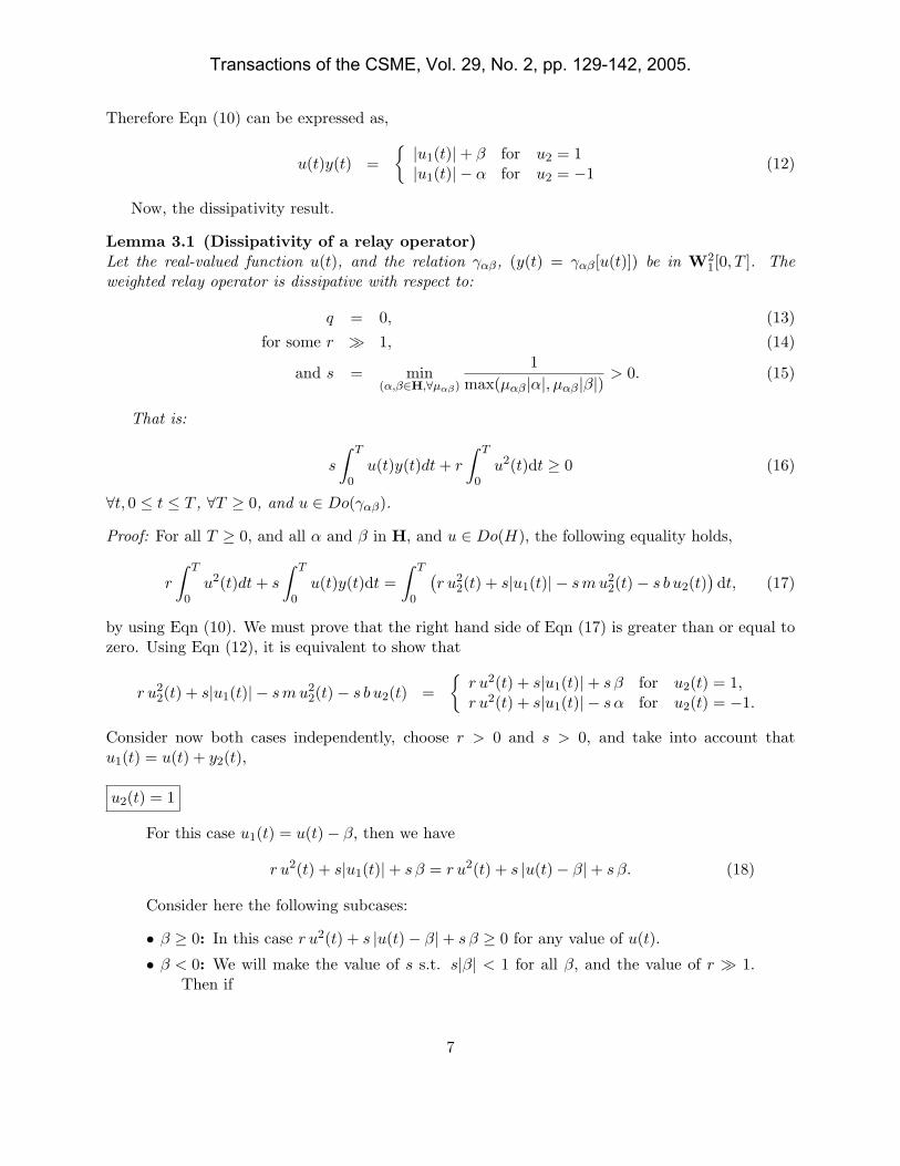
Consider Fig. 5 to be the configuration of the feedback system.

H1

Γu2

u1

y2 e2

e1 y1

H2 = ˆ

Figure 5: Feedback configuration.

Theorem 4.1 (in [12])Suppose that the two subsystems H1 and H2 = Γ are dissipative with respect to supply rates

wi(ui, yi) = y′i qi yi + 2y′i si ui + u′i ri ui, i = 1, 2 (35)

(consider H1 and H2 = to be relations). Then the feedback system is stable (asymptotically stable)if the matrix

Q =[

q1 + αr2 −s1 + αs2

−s1 + αs2 r1 + αq2

](36)

is negative semidefinite (negative definite) for some α > 0.

11


The dissipativity conditions of the previous theorem when H2 is the Preisach model and H1 isthe lead approximation to the phaser are satisfied given the conditions of Section 3. The followingSubsection presents the proof of the stability of the feedback connection of these two subsystems.

4.1 Stability with the Lead Approximation to a Phaser

It was found in the previous section that both the Preisach model and the lead approximationto the phaser are dissipative. It remains to be shown that the matrix Q is negative semidefinite(negative definite) for some α > 0. Also note that since H1 and H2 are relations, the input u2 inFigure 5, will be in W2

1[0, T ] and it will also offset the initial conditions on y1, so that e2 ∈ Do(H2)and the dissipativity of H2 can be exploited.

Let H1 = Lpa and H2 be the Preisach model. From Section 3, it is known that the Preisachmodel is dissipative with respect to q2 = 0, r2 > 0 and s2 = srelay > 0. For the lead approximation,s1 ≥ −q1A− r1B as in (34), q1 ≤ −αr2, and r1 < 0.

Theorem 4.1 can be easily applied if the terms Q12 and Q21 of the matrix Q are equal to zero.This is achieved for an α > 0, if s1 − αs2 = 0 as follows:

α =s1

s2≥ −q1A− r1B

s2

≥ αr2A− r1B

s2since − q1 ≥ αr2

α ≥ −r1B

s2 − r2A, (37)

and since −r1 > 0, we just need to set the value of s2 to be s2 > max{srelay, r2A}, to ensure thatα will be always positive. Then the matrix Q can assume the value

Q =[

q1 + αr2 00 r1

]. (38)

Since r1 < 0, we see that when q1 = −αr2, the matrix is negative semidefinite (eigenvalues smallerthan or equal to zero), and when q1 < −αr2 it is negative definite (eigenvalues smaller than zero).Hence the feedback connection of the lead approximation to the phaser with the Preisach model isstable (asymptotically stable).

5 Conclusion

There is strong experimental evidence that the feedback connection of a system with hysteresis anda lead-type compensator is stable. The lead approximation to the phaser has been used successfullyin the reduction of hysteresis in a piezoceramic actuator [6], and a shape memory alloy actuator[7]. Different types of lead controllers were shown to greatly improve the control of a system withmagnetic hysteresis as reported in [15]. In all these cases, the feedback connection was stable.

Given this evidence, it was felt that it was possible to prove the stability of the Preisach modelwith a certain types of dissipative controllers, and in particular for the lead approximation of aphaser controller. The results obtained for the feedback-equivalent relay operators are of particularinterest and further research should be focused on the stability of the Preisach model with moregeneral classes of feedback controllers.

12


Acknowledgements

The late Prof. G. Zames suggested replacing the relay operator by simpler feedback connections.This research was partly funded by an operating grant from the Natural Sciences and Engineer-

ing Council of Canada and by the Institute for Robotics and Intelligent Systems part of Canada’sCentres of Excellence Program (NCE).

References

[1] B. Boulet, L. K. Daneshmend, V. Hayward, and C. Nemri. System identification and modellingof a high performance hydraulic actuator. In R. Chatila and G. Hirzinger, editors, ExperimentalRobotics 2, Lecture Notes in Control and Information Sciences. Springer Verlag, 1993.

[2] B. M. Chen, T. H. Lee, C. C. Hang, Y. Guo, and S. Weerasooriya. An H∞ almost disturbancedecoupling robust controller design for a piezoelectric bimorph actuator with hysteresis. IEEET. On Control Systems Technology, 7(7):160–194, 1999.

[3] G. S Choi, Y. A. Lim, and G. H. Choi. Tracking position control of piezoelectric actuators forperiodic reference inputs. Mechatronics, 12:669–684, 2002.

[4] M. L. Corradini and G. Parlangeli. Robust stabilization of nonlinear uncertain plants withhysteresis in the actuator: A sliding mode approach. In IEEE Int. Conf. on Systems, Manand Cybernetics, volume 3, pages 500–505, 2002.

[5] J. M. Cruz-Hernandez and V. Hayward. Phase control approach to hysteresis reduction. IEEET. On Control Systems Technology, 9(1):17–26, 2001.

[6] J.M. Cruz-Hernandez and V. Hayward. On the linear compensation of hysteresis. In 36thIEEE Conference on Decision and Control, volume 1, pages 1956–1957, 1997.

[7] J.M. Cruz-Hernandez and V. Hayward. An approach to reduction of hysteresis in smartmaterials. In 1998 IEEE International Conference on Robotics and Automation, pages 1510–1515, 1998.

[8] C.A. Desoer and M. Vidyasagar. Feedback Systems: Input-Output Properties. Academic Press,1975.

[9] S. Fatikow and U. Rembold. Microsystem Technology and Microrobotics. Berlin ; New York :Springer, 1997.

[10] R.B. Gorbet and K.A. Morris. General dissipation in hysteretic systems. In Proceedings of the37th IEEE Conference on Decision and Control, volume 3, pages 4133–4138, 1998.

[11] R.B. Gorbet, K.A. Morris, and D.W.L. Wang. Stability of control for the Preisach hysteresismodel. In Proceedings of the 1997 IEEE International Conference on Robotics and Automation,volume 1, pages 241–247, 1997.

[12] D.J. Hill and P.J. Moylan. Stability results for nonlinear feedback systems. Automatica,13:377–382, 1977.

13


[13] D.J. Hill and P.J. Moylan. Dissipative dynamical systems: Basic input-output and stateproperties. Journal of the Franklin Institute, 309(5):327–357, May 1980.

[14] I.D. Mayergoyz. Mathematical Models of Hysteresis. Springer-Verlag, 1991.

[15] J.-F. Mougenet and V. Hayward. Limit cycle characterization, existence and quenching in thecontrol of high performance hydraulic actuator. In Proc. IEEE International Conference onRobotics and Automation, volume 3, pages 2218–2223, 1995.

[16] S. O. Reza Moheimani and G. C. Goodwin. special issue on dynamics and control of smartstructures. IEEE T. On Control Systems Technology, 9(1), 2001.

[17] A. Sebastian and S. Salapaka. H∞ loop shaping design for nano-positioning. In AmericanControl Conference, volume 5, pages 3708–3713, 2003.

[18] J.J. Slotine and W. Li. Applied Nonlinear Control. Prentice Hall, 1991.

14


Documents

Position Stability For Phase Control Of The Preisach Hysteresis