Embed Size (px)
Citation preview
International Journal of Automation and Computing 10(3), June 2013, 181-193
DOI: 10.1007/s11633-013-0711-3
Position Control of Electro-hydraulic Actuator System
Using Fuzzy Logic Controller Optimized by
Particle Swarm Optimization
Daniel M. Wonohadidjojo1 Ganesh Kothapalli1 Mohammed Y. Hassan2
1School of Engineering, Edith Cowan University, Western Australia 6027, Australia2University of Technology, Baghdad, Iraq (Adjunct Academic, Edith Cowan University, Western Australia 6027, Australia)
Abstract: The position control system of an electro-hydraulic actuator system (EHAS) is investigated in this paper. The EHAS isdeveloped by taking into consideration the nonlinearities of the system: the friction and the internal leakage. A variable load thatsimulates a realistic load in robotic excavator is taken as the trajectory reference. A method of control strategy that is implementedby employing a fuzzy logic controller (FLC) whose parameters are optimized using particle swarm optimization (PSO) is proposed.The scaling factors of the fuzzy inference system are tuned to obtain the optimal values which yield the best system performance. Thesimulation results show that the FLC is able to track the trajectory reference accurately for a range of values of orifice opening. Beyondthat range, the orifice opening may introduce chattering, which the FLC alone is not sufficient to overcome. The PSO optimized FLCcan reduce the chattering significantly. This result justifies the implementation of the proposed method in position control of EHAS.
Keywords: Position control, electro-hydraulic actuator, fuzzy logic controller, particle swarm optimization (PSO), nonlinear.
1 Introduction
Position control applications in most equipment that areimplemented using servo mechanism need a robust controlscheme with tracking accuracy. This requires good position-ing and smooth response of the actuation system. Due totheir capability, electro-hydraulic actuators have been usedin these servo systems for the last few years. Its robustnessand accuracy of position tracking contribute significantlyto the applications and equipment such as robotics, min-ing, and aircraft.
The constraints appearing in the applications of the hy-draulic control system are the internal and external dis-turbances that yield the nonlinearities and uncertainties.Such characteristics emerge on the system and degrade itsperformance significantly. These disturbances have adverseimpact on the robustness and accuracy of position trackingof the system. Such nonlinearities and uncertainties in thehydraulic actuation system are caused by the presence offriction and internal leakage of the system.
The performance of electro-hydraulic actuator system(EHAS) in position control requires an accurate electro-hydraulic actuator which is determined by its positiontracking performance and robustness of the controller.Therefore, the development of such system which guaran-tees the tracking accuracy and robustness is significant.
Nonlinearities and uncertainties in EHAS arise from thefriction and internal fluid leakage in the system. A largenumber of studies have been conducted to overcome theseproblems, in which friction has received more attention. De-spite the less number of studies on the leakage, it cannotbe neglected in practices. Both friction and leakage effectsintroduce chattering which degrades the performance of thesystem in terms of tracking performance and robustness.
Manuscript received May 25, 2012; revised December 3, 2012
A number of studies have been conducted to minimize theimpact of friction and internal leakage. Issues related to thecontrol of the electro-hydraulic actuators was addressed[1],in which a nonlinear model of hydraulic cylinder controlledby servo valves was developed. Specifically, a linearizedmodel of a hydraulic servo system was used to develop a pro-portional, integral and derivative (PID) controller. It alsoutilized the design of feedback linearization controller toovercome some limitations of the linear controllers. This ledto the improved performance of feedback linearization con-trol compared to the PID control. A similar study propos-ing a technique that combined the features of sliding modecontrol and fuzzy control was reported[2]. However, the sys-tems developed in both of these studies still suffered fromchattering. The fuzzy logic was only employed to acceleratethe phase change and attenuate the chattering introducedby the sliding mode control method. In addition, the studydid not take into account the internal fluid leakage in thehydraulic system.
In [3], a technique was proposed for the control of exca-vator dynamics and its hydraulic actuators when executingrobotic excavation tasks involving soil contact operations.The results obtained suggested that the proposed controltechnique can provide robust performance when employedin the automated excavation with soil contact. However,the robustness of this system to the chattering in the hy-draulic actuator was not addressed in this study. The fuzzytuning approach implemented for the control of the ramforce and the cylinder position did not specify the frictionand internal leakage of the excavator hydraulic actuator sys-tem, either.
A self-tuning fuzzy PID controller, developed to improvethe performance of the electro-hydraulic actuator[4], wasbased on the mathematical model of the system. Thismethod used a system identification technique and fuzzy
www.MatlabSite.com | متلب سایت

182 International Journal of Automation and Computing 10(3), June 2013
logic to tune each parameter of the PID controller. How-ever, this study did not consider the load of the hydraulicsystem, the friction in the hydraulic cylinder and the leak-age in the hydraulic actuator system. Another study whichdescribed an application of a fuzzy logic position controlto an electro-hydraulic servo system[5] included a mathe-matical model of that system which considered its internalleakage. However, this work did not take into account theload of the electro-hydraulic system.
An adaptive control scheme was reported in [6] to over-come system uncertainty. This approach used the errorequations for velocity, acceleration and jerk, which weregenerated in the design procedure of the standard back-stepping control scheme. However, a major issue concern-ing the load of the actuator system was not addressed.
In [7], a fuzzy plus proportional integral (PI) controller,which combined fuzzy logic and conventional PI controlwas developed with a fuzzy rule based on the soft-switchmethod. This study did not address specific nonlinearityand uncertainty parameters in the electro-hydraulic system.Furthermore, the switching mechanism used was not testedusing these parameters to verify its robustness and smoothswitching.
In another study, retrofitted electro-hydraulic pilot pro-portional relief valves were developed to effect an excavatorautomatization[8]. This study also developed a model of ex-cavator motion control. The system was used to handle thenonlinearity, parameter uncertainties and external distur-bances. However, questions were raised over the system′srobustness, because the study did not specify the nonlin-earities and parameter uncertainties that emerged in thesystem.
A sliding mode control (SMC) with fixed and varyingboundary layers was proposed[9]. The controller schemewas employed to control the position tracking performanceof an electro-hydraulic actuator system. It was aimed tocompensate for nonlinearities and uncertainties caused bythe presence of friction and internal leakage, and this studyalso considered a fixed load for the system. However, thechattering in the SMC′s control signals, due to the discon-tinuous term in its control law, was not overcome.
An available nonlinear observer for Coulomb friction wasmodified to simultaneously estimate friction, velocity, andacceleration. This scheme was investigated in [10]. Anobserver-based friction compensating control strategy wasdeveloped to improve tracking performance of the manipu-lator. This study did not take into consideration the leakagethat emerged in the electro-hydraulic system.
In this paper, a method to control the position of electro-hydraulic servo system is proposed. The objective of thisstudy is to develop a method of position control of theEHAS using an intelligent controller. The controller is ro-bust to the nonlinearities and uncertainties that emerge inthe system. The position tracking should be able to findthe optimum parameters of the controller so that the errorin position and chattering are minimized. The developmentof that method includes several steps. First, a fuzzy logiccontroller (FLC) is designed as the controller of the non-linear model of electro-hydraulic system. The model takesinto consideration the friction and internal leakage. Then,the unoptimized FLC is employed and the system response
is observed with computer simulation. Next, parameters ofthe FLC are optimized by the particle swarm optimization(PSO) algorithm. The optimized parameters are the scalingfactors of the fuzzy inference system. When the optimizedparameters are obtained, the performance and robustnessof the unoptimized and optimized FLC is compared. Theoptimization is confirmed through computer simulation.
Despite the wide range of applications of EHAS in in-dustries, aircraft, robotics and machinery, it will be inves-tigated by taking into consideration the use of EHAS inexcavators in this paper.
The paper is organized as follows. Section 2 describes themathematical models to develop the electro-hydraulic servosystem with the complete Simulink model presented at theend of this section. The FLC design is explained in Section3. Then, we explain the PSO in Section 4. The testing andsimulations of the position control of the electro-hydraulicactuator system are presented in Section 5 followed by theresults and discussion in Section 6. We then conclude ourstudy in Section 7.
2 Electro-hydraulic actuator system
2.1 Hydraulic dynamics and force balancemodel
The electro-hydraulic actuator system modelled in thisstudy consists of two main parts: the valve and the cylinder.The cylinder is modelled as a double acting single rod orsingle ended piston, with a single load attached at the endof the piston. The cylinder is depicted in Fig. 1[11].
Fig. 1 Electro-hydraulic cylinder
In Fig. 1, Xp is the cylinder position, F denotes the ap-plied load to the cylinder, Q1 and Q2 are the fluid flow toand from the cylinder, respectively. P1 is the fluid pres-sure within side 1 and P2 is the fluid pressure within side2. The pressurized areas on side 1 and side 2 are A1 andA2, respectively. The cylinder will retract or extend whena pressure difference between P1 and P2 occurs.
The dynamics of the system is expressed by
Xp = Vp (1)
map = Fa − Ff (2)
where Xp is the piston position, Vp is the piston velocity,ap is the piston acceleration, and m is the piston and loadmass. There are two forces in (2) that influence the system:the hydraulic actuating force Fa and the friction force Ff
which are functions of nonlinearities that will significantlyinfluence the system. The parameters that affect Fa are thecontrol input voltage, environment load, cylinder pressure,
www.MatlabSite.com | متلب سایت
D. M. Wonohadidjojo et al. / Position Control of Electro-hydraulic Actuator System · · · 183
friction force and leakage. Hence, it can be represented by
Fa = ApPl. (3)
Therefore, the force balance equality of the cylinder is rep-resented by
map = ApPl − Ff (4)
where Ap is the cross section of the hydraulic cylinder, andPl is the cylinder differential pressure written as
Pl = P1 − P2. (5)
Equality (4) represents the dynamics of the system.As discussed in [9], by defining the load pressure Pl to
be the pressure across the actuator piston, the derivativeof the load pressure is given by the total load flow throughthe actuator divided by the fluid capacitance as
Vt
βePl = Ql − CtPl −ApVp (6)
where Vt is the total actuator volume of both cylinder sides,βe is the bulk modulus of hydraulic oil, Ct is the total leak-age coefficient, and Ql is the load flow. By using (6), theflow equality of the servo valve is given in (7), which ex-presses the relationship between spool valve displacementXv and the load flow Ql.
QL = Cdwxv
√ps − sgn(xv)pl
ρ(7)
where Cd is discharge coefficient, W is the spool valve areagradient, Ps is the supply pressure, and ρ is the oil den-sity. Substituting (7) into (6), one can find the hydraulicsdynamics of the cylinder pressure as
Pl =4βe
Vt
[−Apvp − ctpl + Cdwxv
√Ps − sgn(xv)pl
ρ
].
(8)
The spool displacement of the servo valve Xv is controlledby the control signal generated by the FLC u. The corre-sponding relation can be simplified to
Xv =1
τv(−xv + kvu). (9)
The servo valve input can also be expressed as a secondorder equation as
U =1
kv
(1
ω2v
xv +2DRv
ωvxv + xv
)(10)
where kv is the servo valve gain, τv is the time constant,ωv is the natural frequency, and DRV is the damping ratioof servo valve. Based on (1)–(10), if the state variables aredetermined as
x = [x1, x2, x3]T = [xp, vp, ap]T (11)
then a third order state equation model for the servo hy-draulic actuator system can be obtained by replacing thevalve dynamics (9) with
xv = kvu. (12)
Then, the following equalites can be obtained as
x1 = x2 (13)
x2 = x3 (14)
X3 = ap =1
m(Appl − Ff ). (15)
2.2 Friction model
Friction is an important aspect of many control systemsboth for high quality servo mechanisms and simple pneu-matic and hydraulic systems. Friction can lead to track-ing errors, limit cycles, and undesired stick-slip motion[12].Friction is the tangential reaction force between two sur-faces in contact. Physically, these reaction forces are theresults of many different mechanisms, which depend on con-tact geometry and topology, properties of the bulk and sur-face materials of the bodies, displacement and relative ve-locity of the bodies, and presence of lubrication[6].
The commonly used model for friction is usually depictedby the discontinuous static mapping between velocity andfriction force. This needs to consider the Coulomb and vis-cous friction that depends on the velocity sign. The staticmodel, however, does not take into consideration the dy-namics behavior of the friction force, such as stick-slip mo-tion, re-sliding displacement and friction lag. These char-acteristics are properties of friction in nature. Therefore,friction does not have instantaneous response to the veloc-ity change.
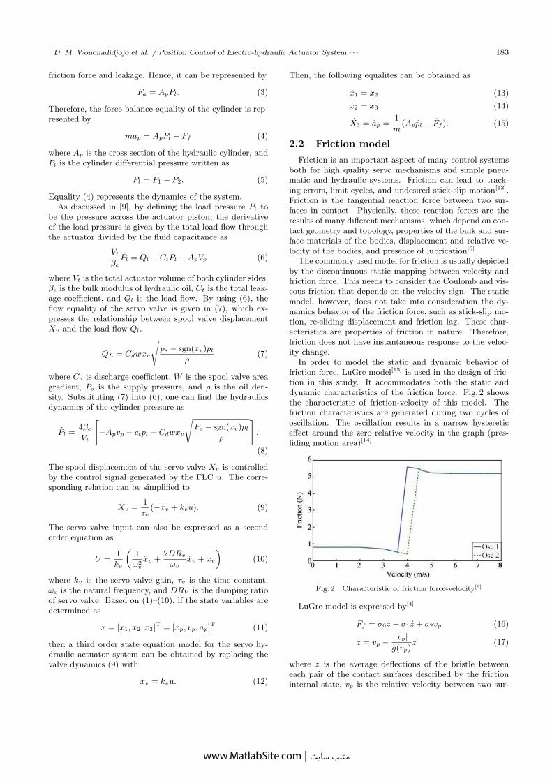
In order to model the static and dynamic behavior offriction force, LuGre model[13] is used in the design of fric-tion in this study. It accommodates both the static anddynamic characteristics of the friction force. Fig. 2 showsthe characteristic of friction-velocity of this model. Thefriction characteristics are generated during two cycles ofoscillation. The oscillation results in a narrow hystereticeffect around the zero relative velocity in the graph (pres-liding motion area)[14].
Fig. 2 Characteristic of friction force-velocity[9]
LuGre model is expressed by[4]
Ff = σ0z + σ1z + σ2vp (16)
z = vp − |vp|g(vp)
z (17)
where z is the average deflections of the bristle betweeneach pair of the contact surfaces described by the frictioninternal state, vp is the relative velocity between two sur-
www.MatlabSite.com | متلب سایت

184 International Journal of Automation and Computing 10(3), June 2013
faces σ0, σ1, and σ2 are the stiffness of the bristle betweentwo contact surfaces, the bristles damping coefficient, andthe viscous friction coefficient, respectively. The nonlinearproperty of friction is described by g(vp) in (18), which canbe parameterized to characterize the Stribeck effect.
g(vp) =1
σ0
[Fc + (Fs − Fc)e
−( vp
vs
)2](18)
where Fc, Fs and vs are the Coulomb friction, viscous fric-tion and stribeck velocity, respectively.
2.3 Internal leakage model
At small servo valve spool displacements, the leakage flowbetween the valve spool and body dominates the orifice flowthrough the valve[15]. In precision positioning applications,where the servo valve operates within the null region, thisflow, if ignored, may severely degrade the performance of aconventional servo hydraulic design.
In this study, an accurate model of leakage flow[15] thattakes into consideration the leakage flow and orifice flow isapplied. By making smooth transition between them wouldlikely improve the precision of the servo hydraulic systemdesign and performance. The model used is a nonlinearservo valve model that accurately captures the servo valveleakage behavior over the whole range of spool movement.The leakage behavior is modeled as turbulent flow with aflow area inversely proportional to the overlap between thespool areas and the servo valve orifices.
A servo valve configuration depicted in Fig. 3 consists oftwo control ports with variable orifices which regulate theflow rates. The flow rates through the control ports of theservo valve are expressed in (19), and the flow rate at thesupply and return ports are represented in (20).
Q1 = QIS −QIR and Q2 = Q2R −Q2S (19)
QS = QIS + Q2S and QR = QIR −Q2R. (20)
Fig. 3 Hydraulic servo valve configuration
The flow rates at the supply side and return side of con-trol port 1 are given by
QIS = KIS
√PS − PIX0 + Xv), Xv 6 0 (21)
QIR = KIR
√PI − PRX2
0 (X0 + kIRXv)−1, Xv > 0 (22)
where X0 is the leakage flow rate at null (Xv = 0). X0
is equivalent to a spool displacement that would result inthe same amount of flow in a nonleaking servo valve as the
leakage flow rate in a leaking servo valve with a centeredspool. Since the leakage resistance increases at larger valveopenings, the leakage flow rate is inversely proportional tothe spool displacement[15].
The relations for orifice and leakage flow at the servovalve ports form the basis of the servo valve flow model.For a negative spool displacement, the flow relations areinterchanged since now the supply side forms the leakagepath and the return side flow is an orifice flow. Applyingsimilar reasoning to each orifice, we obtain the flow relationsfor control port 1[15] as
QIS = KIS(PS − PI)12
{(X0 + XV ), XV > 0
X20 (X0 − kISXV )−1, XV < 0
(23)
QIR = KIR(PI − PR)12
{X2
0 (X0 + kIRXV )−1, XV > 0
X0 −XV , XV < 0.
(24)
For control port 2, the flow relations are
Q2S = K2S(PS − P2)12
{X2
0 (X0 − k2SXV )−1, XV > 0
(X0 −XV ), XV < 0.
(25)
Q2R = K2R(P2 − PR)12
{(X0 + XV ), XV > 0
X20 (X0 − k2RXV )−1, XV < 0.
(26)
The total supply flow QS represents the internal leakageflow since the control ports are blocked for an internal leak-age test[5]. The internal leakage flow can be expressed by
QS = 2Kf (PS − PR)2(X0 + |XV |)(1 + f(X))2 (27)
where
f(Xv) =
[1 +
|Xv|X0
]2 [1 + kf
|Xv|X0
]2
. (28)
Having discussed the electro-hydraulic actuator model,the friction model, and the internal leakage model, we thenintegrate them into an integrated model. The friction modelis integrated by supplying the output of (16)–(18) into themodel. The internal leakage model in (23)–(27) are inte-grated into (6)–(7) to determine the total supply flow intoside 1 of the cylinder.
The parameters and values of the system are listed inTable l. The servo valve and hydraulic cylinder parametersare obtained from the physical system in [9]. The compat-ibility of these subsystems has been verified in simulationsas well as experimental tests in that study.
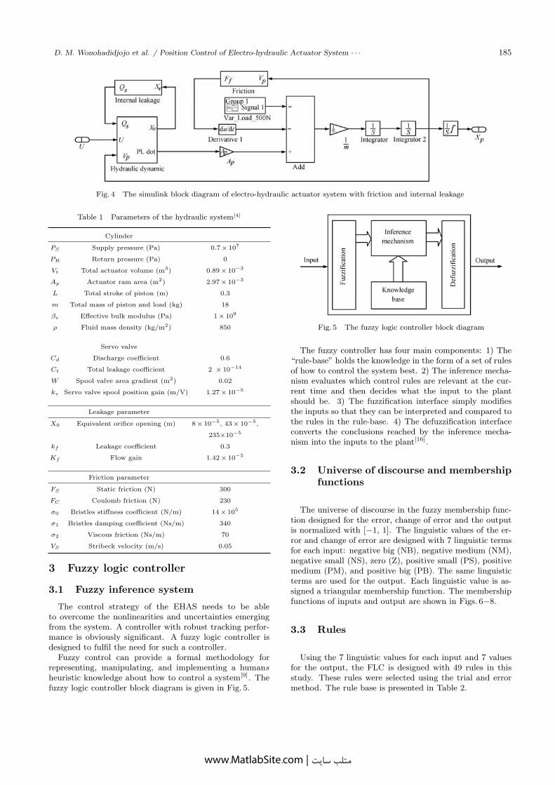
The Simulink block diagram of the electro-hydraulicservo system with friction and internal leakage modeledfrom (1)–(28) is shown in Fig. 4. The next section willdiscuss the FLC used to control the position of electro-hydraulic system (EHS) model that contains friction andinternal leakage.
www.MatlabSite.com | متلب سایت
D. M. Wonohadidjojo et al. / Position Control of Electro-hydraulic Actuator System · · · 185
Fig. 4 The simulink block diagram of electro-hydraulic actuator system with friction and internal leakage
Table 1 Parameters of the hydraulic system[4]
Cylinder
PS Supply pressure (Pa) 0.7× 10⁷
PR Return pressure (Pa) 0
Vt Total actuator volume (m3) 0.89× 10⁻³
Ap Actuator ram area (m2) 2.97× 10⁻³
L Total stroke of piston (m) 0.3
m Total mass of piston and load (kg) 18
βe Effective bulk modulus (Pa) 1× 10⁹
ρ Fluid mass density (kg/m2) 850
Servo valve
Cd Discharge coefficient 0.6
Ct Total leakage coefficient 2 × 10⁻¹⁴
W Spool valve area gradient (m2) 0.02
kv Servo valve spool position gain (m/V) 1.27× 10⁻⁵
Leakage parameter
X0 Equivalent orifice opening (m) 8× 10⁻⁵, 43× 10−5,
235×10−5
kf Leakage coefficient 0.3
Kf Flow gain 1.42× 10⁻⁵
Friction parameter
FS Static friction (N) 300
FC Coulomb friction (N) 230
σ0 Bristles stiffness coefficient (N/m) 14× 105
σ1 Bristles damping coefficient (Ns/m) 340
σ2 Viscous friction (Ns/m) 70
VS Stribeck velocity (m/s) 0.05
3 Fuzzy logic controller
3.1 Fuzzy inference system
The control strategy of the EHAS needs to be ableto overcome the nonlinearities and uncertainties emergingfrom the system. A controller with robust tracking perfor-mance is obviously significant. A fuzzy logic controller isdesigned to fulfil the need for such a controller.
Fuzzy control can provide a formal methodology forrepresenting, manipulating, and implementing a humansheuristic knowledge about how to control a system[9]. Thefuzzy logic controller block diagram is given in Fig. 5.
Fig. 5 The fuzzy logic controller block diagram
The fuzzy controller has four main components: 1) The“rule-base” holds the knowledge in the form of a set of rulesof how to control the system best. 2) The inference mecha-nism evaluates which control rules are relevant at the cur-rent time and then decides what the input to the plantshould be. 3) The fuzzification interface simply modifiesthe inputs so that they can be interpreted and compared tothe rules in the rule-base. 4) The defuzzification interfaceconverts the conclusions reached by the inference mecha-nism into the inputs to the plant[16].
3.2 Universe of discourse and membershipfunctions
The universe of discourse in the fuzzy membership func-tion designed for the error, change of error and the outputis normalized with [−1, 1]. The linguistic values of the er-ror and change of error are designed with 7 linguistic termsfor each input: negative big (NB), negative medium (NM),negative small (NS), zero (Z), positive small (PS), positivemedium (PM), and positive big (PB). The same linguisticterms are used for the output. Each linguistic value is as-signed a triangular membership function. The membershipfunctions of inputs and output are shown in Figs. 6−8.
3.3 Rules
Using the 7 linguistic values for each input and 7 valuesfor the output, the FLC is designed with 49 rules in thisstudy. These rules were selected using the trial and errormethod. The rule base is presented in Table 2.
www.MatlabSite.com | متلب سایت

186 International Journal of Automation and Computing 10(3), June 2013
Fig. 6 Membership functions of error as input
Fig. 7 Membership functions of change of error as input
Fig. 8 Membership functions of control signal as output
Table 2 Rule base of the FLC
E PB PM PS Z NS NM NB
∆ E
PB PB PB PM PM PS PS Z
PM PB PM PM PS PS Z NS
PS PM PM PS PS PZ NS NS
Z PM PS PS Z NS NS NM
NS PS PS Z NS NS NM NB
NM PS Z NS NS NM NB NB
NB Z NS NS NM NB NB NB
3.4 PI-like FLC
The FLC is designed as a PI fuzzy logic controller wherethe equality of the PI-controller is
du = Ki × e(t) + Kp × de
dt(29)
with
u = u0 + Ku × du (30)
where Kp and Ki are the proportional and the integral gaincoefficients, respectively, u0 is the output of the controllerin the previous sampling time and Ku is the output scalingfactor. A block diagram for a PI like fuzzy logic controlsystem is depicted in Fig. 9[17].
Fig. 9 Block diagram of a PI-like fuzzy logic control system
Based on Fig. 9, it is clear that the FLC has two inputvariables: error and change of error. The output variableof the controller is the control signal to control the plant.Thus, the FLC is a two-inputs and one-output system.
After the design of FLC, it is connected with the plantwhich is the integrated model of the electro-hydraulic sys-tem to be controlled. This forms a closed loop system withthe FLC as the controller, and the output of the plant isobserved as the feedback to control system. The system out-put is denoted by y(t), its inputs are denoted by u(t), andthe reference input to the fuzzy logic controller is denotedby r(t) as shown in Fig. 10. The Simulink block diagram ofthe closed loop system is depicted in Fig. 11.
Fig. 10 Fuzzy logic controlled integrated hydraulic model in a
closed-loop control system
Fig. 11 Simulink block of the FLC controlled integrated EHAS
in closed loop system
3.5 FLC tuning
The rest of the process will be the simulation of thewhole system and the tuning of the FLC. The objective isto obtain the best system performance. This can be accom-plished by tuning the values of scaling factors: Kp, Ki andKu that can result in the minimum oscillation, overshootand error in position.
Tuning of FLC parameters using the trial and errormethod does not always give the optimum results. In ad-
www.MatlabSite.com | متلب سایت
D. M. Wonohadidjojo et al. / Position Control of Electro-hydraulic Actuator System · · · 187
dition, it is a time consuming process. Therefore, an intel-ligent optimization technique to optimize the FLC param-eters is obviously necessary. The next section discusses theparticle swarm optimization.
4 Particle swarm optimization
In 1995, Kennedy and Eberhart introduced particleswarm optimization as an evolutionary algorithm. PSO wasinspired by swarming behaviors observed in flocks of birds,schools of fish, or swarms of bees. PSO is a population-based optimization tool, which could be implemented andapplied to solve various function optimization problems, orthe problems that can be transformed to function optimiza-tion problems. This method was developed through simu-lation of a simplified social system, and has been foundto be robust in solving continuous nonlinear optimizationproblems[18].
In PSO, each particle is attracted toward the positionof current global best g∗ and its own best location x∗i inhistory, and at the same time, it has tendency to move ran-domly. When a particle finds a location that is better thanpreviously found locations, then it updates the location asthe new current best location for particle i. There is a cur-rent best location for all n particles at any time t duringiterations. The aim is to find the global best solution amongall the current best solutions until the objective no longerimproves or after a certain number of iterations. The es-sential steps of the PSO can be summarized as the pseudocode[13]:
Particle swarm optimizationObjective function f(x), x = (x1, · · · , xp)1
Initialize locations xi and velocities vi of n particlesFind g∗ from min {f(x1), · · · , f(xn)}(at t = 0)While (criterion)
T = t + 1 (pseudo time or iteration counter)For loop over all n particles and all d dimensions
Generate new velocity vt+1i using (30)
Evaluate objective functions at new locations xt+1i
Find the current best location for each particle x∗iEnd forFind the current global best g∗
End while
Output the final results x∗i and g∗
When xi and vi are the position vector and velocity forparticle i, the new vector is determined by
vt+1i = vt
i + α1 × [g∗ − xt+1i ] + β2 × [xi − xt
i] (31)
where α1 and β2 are two random vectors, and each entrytakes the value between 0 and 1. Parameters α and β arethe learning parameters or acceleration constants, whichcan be typically taken as 2[19].
4.1 Accelerated PSO
The accelerated PSO based on [19] is employed in thisstudy. The standard PSO uses both the current global bestg∗ and the individual best x∗i . The reason of using the indi-vidual best particle is primarily to increase the diversity inthe quality solutions. However, this diversity can be sim-ulated using some randomness. Subsequently, there is nocompelling reason for using the individual best particle, un-less the optimization problem of interest is highly nonlinearand multimodal[19].
As discussed in [19], a simplified version which could ac-celerate the convergence of the algorithm is to use the globalbest particle only. Thus, in the accelerated PSO, the veloc-ity vector is generated by E
vt+1i = vt
i + α
(E − 1
2
)+ β(g∗ − xt
i) (32)
where E is a random variable with values ranging from 0to 1. We can also use a standard normal distribution αEn,where En is drawn from N(0, 1) to replace the second term.The update of the position is
xt+1i = xt
i + vt+1i . (33)
In order to increase the convergence even further, the up-date of the location in a single step can also be writtenas
xt+1i = (1− β)xt
i + βg∗ + αEn. (34)
This simpler version will give the same order of conver-gence. The typical values for this accelerated PSO areα ≈ 0.1 ∼ 0.7, though α ≈ 0.2 and β ≈ 0.5 can be takenas the initial values for most unimodal objective functions.It is worth pointing out that parameters α and β shouldbe related to the scales of the independent variables xi andthe search domain in general.
A further improvement to the accelerated PSO used in[19] is to reduce the randomness as iterations proceed. Thismeans that we can use a monotonically decreasing functionsuch as
α = α0e−γt (35)
or
α = α0γt, 0 < γ < 1 (36)
where α ≈ 0.5 ∼ 1 is the initial value of the randomnessparameter. Here, t is the number of iterations or time steps,0 < γ < 1 is a control parameter, where t ∈ [0, 10]. Ob-viously, these parameters are fine-tuned to suit the currentoptimization problem.
4.2 PSO implementation
The parameters used in the PSO are as follows:Number of particles: 25,Dimension of the problem: 3,Number of maximum iterations: 500,Speed of convergence (β = acceleration coefficient deter-
mining the scale of the forces in the direction of pi): 0.5,Randomness amplitude of roaming particles (α = accel-
eration coefficient determining the scale of the forces in thedirection of gi): 0.2,
γ = 0.95.The PSO is employed to optimize the FLC parameters
(scaling factors): Ki, Kp, Ku. These factors are optimizedat the same time. The function of these parameters in theFLC is shown as
∆u(t) = Ki × e(t) + Kp ×∆e(t). (37)
www.MatlabSite.com | متلب سایت
188 International Journal of Automation and Computing 10(3), June 2013
The fitness function of the problem is the integral of timemultiplied by absolute errors (ITAE) as
IITAE =
∫ T
0
t|e(t)|dt. (38)
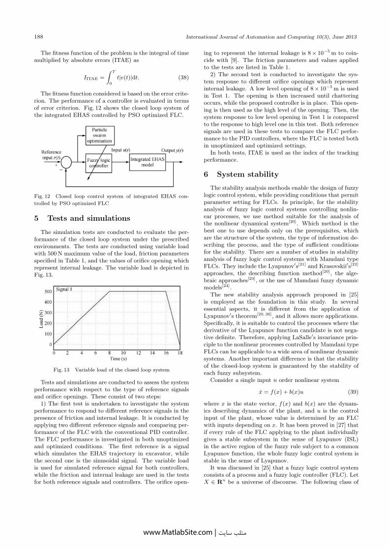
The fitness function considered is based on the error crite-rion. The performance of a controller is evaluated in termsof error criterion. Fig. 12 shows the closed loop system ofthe integrated EHAS controlled by PSO optimized FLC.
Fig. 12 Closed loop control system of integrated EHAS con-
trolled by PSO optimized FLC
5 Tests and simulations
The simulation tests are conducted to evaluate the per-formance of the closed loop system under the prescribedenvironments. The tests are conducted using variable loadwith 500 N maximum value of the load, friction parametersspecified in Table 1, and the values of orifice opening whichrepresent internal leakage. The variable load is depicted inFig. 13.
Fig. 13 Variable load of the closed loop system
Tests and simulations are conducted to assess the systemperformance with respect to the type of reference signalsand orifice openings. These consist of two steps:
1) The first test is undertaken to investigate the systemperformance to respond to different reference signals in thepresence of friction and internal leakage. It is conducted byapplying two different reference signals and comparing per-formance of the FLC with the conventional PID controller.The FLC performance is investigated in both unoptimizedand optimized conditions. The first reference is a signalwhich simulates the EHAS trajectory in excavator, whilethe second one is the sinusoidal signal. The variable loadis used for simulated reference signal for both controllers,while the friction and internal leakage are used in the testsfor both reference signals and controllers. The orifice open-
ing to represent the internal leakage is 8× 10⁻⁵ m to coin-cide with [9]. The friction parameters and values appliedto the tests are listed in Table 1.
2) The second test is conducted to investigate the sys-tem response to different orifice openings which representinternal leakage. A low level opening of 8× 10⁻⁵ m is usedin Test 1. The opening is then increased until chatteringoccurs, while the proposed controller is in place. This open-ing is then used as the high level of the opening. Then, thesystem response to low level opening in Test 1 is comparedto the response to high level one in this test. Both referencesignals are used in these tests to compare the FLC perfor-mance to the PID controllers, where the FLC is tested bothin unoptimized and optimized settings.
In both tests, ITAE is used as the index of the trackingperformance.
6 System stability
The stability analysis methods enable the design of fuzzylogic control system, while providing conditions that permitparameter setting for FLCs. In principle, for the stabilityanalysis of fuzzy logic control systems controlling nonlin-ear processes, we use method suitable for the analysis ofthe nonlinear dynamical system[20]. Which method is thebest one to use depends only on the prerequisites, whichare the structure of the system, the type of information de-scribing the process, and the type of sufficient conditionsfor the stability. There are a number of studies in stabilityanalysis of fuzzy logic control systems with Mamdani typeFLCs. They include the Lyapunov′s[21] and Krasovskii′s[22]
approaches, the describing function method[20], the alge-braic approaches[23], or the use of Mamdani fuzzy dynamicmodels[24].
The new stability analysis approach proposed in [25]is employed as the foundation in this study. In severalessential aspects, it is different from the application ofLyapunov′s theorem[20, 26], and it allows more applications.Specifically, it is suitable to control the processes where thederivative of the Lyapunov function candidate is not nega-tive definite. Therefore, applying LaSalle′s invariance prin-ciple to the nonlinear processes controlled by Mamdani typeFLCs can be applicable to a wide area of nonlinear dynamicsystems. Another important difference is that the stabilityof the closed-loop system is guaranteed by the stability ofeach fuzzy subsystem.
Consider a single input n order nonlinear system
x = f(x) + b(x)u (39)
where x is the state vector, f(x) and b(x) are the dynam-ics describing dynamics of the plant, and u is the controlinput of the plant, whose value is determined by an FLCwith inputs depending on x. It has been proved in [27] thatif every rule of the FLC applying to the plant individuallygives a stable subsystem in the sense of Lyapunov (ISL)in the active region of the fuzzy rule subject to a commonLyapunov function, the whole fuzzy logic control system isstable in the sense of Lyapunov.
It was discussed in [25] that a fuzzy logic control systemconsists of a process and a fuzzy logic controller (FLC). LetX ∈ Rn be a universe of discourse. The following class of
www.MatlabSite.com | متلب سایت

D. M. Wonohadidjojo et al. / Position Control of Electro-hydraulic Actuator System · · · 189
single input nonlinear dynamical systems modeled by thestate-space equations is accepted.
x = f(x) + b(x)u (40)
where x ∈ X, x = [x1 x2 · · ·xn]T is the state vector, and
x = [x1 x2 · · · xn]T (41)
is the derivative of x with respect to the time variable t,
b(x) = [b1(x) b2(x) · · · bn(x)]T (42)
are functions describing the dynamics of the process, and uis the control signal fed to the process, obtained by the cen-tre of gravity (COG) defuzzification method for Mamdanitype fuzzy logic.
In [25], it was proved that if each subsystem is stable inthe sense of Lyapunov. Under a common Lyapunov func-tion, the overall system will be also stable in the sense ofLyapunov. In these conditions, it is guaranteed that theequilibrium point at the origin is globally asymptoticallystable. Theorem 1 in [25] states that if P is a positive defi-nite matrix and
1) V (x) = xTPx →∼ as ||x|| →∼, V (0) = 0.2) V (x) 6 0, ∀x ∈ X for all fuzzy subsystems.3) The set {x ∈ X|V (X) = 0} contains no trajectory of
the system except the trivial trajectory x(t) = 0 for t > 0,then, a fuzzy logic controller with the AND-SUM-COG isglobally asymptotically stable at the origin.
The fuzzy logic controller defined in Section 3 with AND-SUM-COG can fulfill the one defined in [25, 27]. Accordingto Theorem 1 in [25] and Lemma 3.1 in [27], the closedloop system in Fig. 10 is then simulated to analyse the re-sponse. The simulation result is depicted in Fig. 14. Theresult shows that input, output and the control signal con-verge for t > 0. This indicates that the fuzzy logic controlsystem is globally asymptotically stable.
Fig. 14 Response of the system stability test
7 Results and discussion
By applying simulated reference input with 8× 10⁻⁵ morifice opening, Figs. 15 and 16 show the responses of thesystems using the unoptimized FLC and PID controllers, re-spectively. It can be observed that the FLC is able to trackthe reference accurately without overshoot, chattering andsteady state error, so that it does not need to be optimized.The ITAE of this test is 0.0089. The PID controller tracks
the reference with a delay time up to 2 s, overshoot of 5%and ITAE of 0.4904. It can also be assessed, that the ITAEfor PID is higher than the one for FLC with significantdifference. This indicates that the performance of FLC isbetter than that of the PID in this test.
Fig. 15 Response of the system using unoptimized FLC with
simulated reference signal and 8× 10⁻⁵ m orifice opening
Fig. 16 Response of the system using PID controller with sim-
ulated reference signal and 8× 10⁻⁵ m orifice opening
Using the same orifice opening and friction parameters,both of the controllers are tested with sinusoidal signal ref-erence. Position response of the system for unoptimizedFLC and PID controllers are shown in Figs.17 and 18, re-spectively. It can be seen from Fig. 17 that the unopti-mized FLC performs satisfactorily to track the referencewithout errors, delay and chattering. The ITAE of this testis 0.0164. Fig. 18 shows that although the PID controller isable to track the position reference, it still introduces delaybetween 0 s and 2 s, where the ITAE of this test is 0.8114.
Fig. 17 Response of the system using unoptimized FLC with
sinusoidal reference and 8× 10⁻⁵ m orifice opening
The second test is conducted for both FLC and PID con-
www.MatlabSite.com | متلب سایت
190 International Journal of Automation and Computing 10(3), June 2013
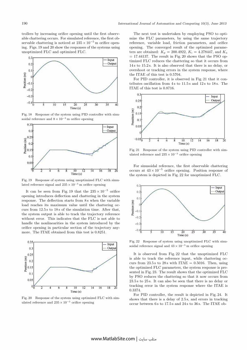
trollers by increasing orifice opening until the first observ-able chattering occurs. For simulated reference, the first ob-servable chattering is noticed at 235× 10−5 m orifice open-ing. Figs. 19 and 20 show the responses of the systems usingunoptimized FLC and optimized FLC.
Fig. 18 Response of the system using PID controller with sinu-
soidal reference and 8× 10⁻⁵ m orifice opening
Fig. 19 Response of system using unoptimized FLC with simu-
lated reference signal and 235× 10−5 m orifice opening
It can be seen from Fig. 19 that the 235× 10−5 orificeopening introduces deflection and chattering in the systemresponse. The deflection starts from 8 s when the variableload reaches its maximum value until the chattering oc-curs from 12.5 s to 18 s of the simulation time. After that,the system output is able to track the trajectory referencewithout error. This indicates that the FLC is not able tohandle the nonlinearities in the system introduced by theorifice opening in particular section of the trajectory any-more. The ITAE obtained from this test is 0.8251.
Fig. 20 Response of the system using optimized FLC with sim-
ulated reference and 235× 10−5 orifice opening
The next test is undertaken by employing PSO to opti-mize the FLC parameters, by using the same trajectoryreference, variable load, friction parameters, and orificeopening. The converged result of the optimized parame-ters are obtained: Kp = 200.4922, Ki = 4.278447, and Ku
= 17.44137. The result in Fig. 20 shows that the PSO op-timized FLC reduces the chattering so that it occurs from14 s to 15.2 s. It is also observed that there is no delay, orovershoot or tracking errors in the system response, wherethe ITAE of this test is 0.5704.
For PID controller, it is observed in Fig. 21 that it con-tributes oscillation from 4 s to 11.5 s and 12 s to 18 s. TheITAE of this test is 0.8716.
Fig. 21 Response of the system using PID controller with sim-
ulated reference and 235× 10−5 orifice opening
For sinusoidal reference, the first observable chatteringoccurs at 43× 10−5 orifice opening. Position response ofthe system is depicted in Fig. 22 for unoptimized FLC.
Fig. 22 Response of system using unoptimized FLC with sinu-
soidal reference signal and 43× 10−5 m orifice opening
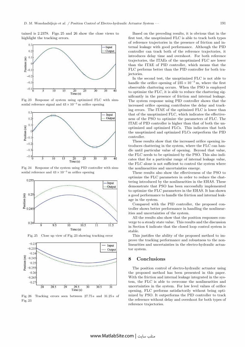
It is observed from Fig. 22 that the unoptimized FLCis able to track the reference input, while chattering oc-curs from 23.5 s to 28 s with ITAE = 0.5016. Then, usingthe optimized FLC parameters, the system response is pre-sented in Fig. 23. The result shows that the optimized FLCby PSO reduces the chattering so that it now occurs from23.5 s to 25 s. It can also be seen that there is no delay ortracking error in the system response where the ITAE is0.3374.
For PID controller, the result is depicted in Fig. 24. Itshows that there is a delay of 2.5 s, and errors in trackingoccur between 6 s to 17.5 s and 24 s to 36 s. The ITAE ob-
www.MatlabSite.com | متلب سایت
D. M. Wonohadidjojo et al. / Position Control of Electro-hydraulic Actuator System · · · 191
tained is 2.2378. Figs. 25 and 26 show the close views tohighlight the tracking errors.
Fig. 23 Response of system using optimized FLC with sinu-
soidal reference signal and 43× 10−5 m orifice opening
Fig. 24 Response of the system using PID controller with sinu-
soidal reference and 43× 10−5 m orifice opening
Fig. 25 Close up view of Fig. 23 showing tracking error
Fig. 26 Tracking errors seen between 27.75 s and 31.25 s of
Fig. 23
Based on the preceding results, it is obvious that in thefirst test, the unoptimized FLC is able to track both typesof reference trajectories in the presence of friction and in-ternal leakage with good performance. Although the PIDcontroller can track both of the reference trajectories, itintroduces delay time and overshoot. For both referencetrajectories, the ITAEs of the unoptimized FLC are lowerthan the ITAE of PID controller, which means that theFLC performs better than the PID controller for both tra-jectories.
In the second test, the unoptimized FLC is not able tohandle the orifice opening of 235× 10−5 m, where the firstobservable chattering occurs. When the PSO is employedto optimize the FLC, it is able to reduce the chattering sig-nificantly in the presence of friction and internal leakage.The system response using PID controller shows that theincreased orifice opening contributes the delay and track-ing errors. The ITAE of the optimized FLC is lower thanthat of the unoptimized FLC, which indicates the effective-ness of the PSO to optimize the parameters of FLC. TheITAE of PID controller is higher than that of both the un-optimized and optimized FLCs. This indicates that boththe unoptimized and optimized FLCs outperform the PIDcontroller.
These results show that the increased orifice opening in-troduces chattering in the system, where the FLC can han-dle until particular value of opening. Beyond that value,the FLC needs to be optimized by the PSO. This also indi-cates that for a particular range of internal leakage value,the FLC alone is not sufficient to control the system wherethe nonlinearities and uncertainties emerge.
These results also show the effectiveness of the PSO tooptimize the FLC parameters in order to reduce the chat-tering introduced by the nonlinearities in the EHAS. Thesedemonstrate that PSO has been successfully implementedto optimize the FLC parameters in the EHAS. It has showna good performance to handle the friction and internal leak-age in the system.
Compared with the PID controller, the proposed con-troller shows better performance in handling the nonlinear-ities and uncertainties of the system.
All the results also show that the position responses con-verge to a steady state value. This results and the discussionin Section 6 indicate that the closed loop control system isstable.
This justifies the ability of the proposed method to im-prove the tracking performance and robustness to the non-linearities and uncertainties in the electro-hydraulic actua-tor system.
8 Conclusions
The position control of electro-hydraulic actuator usingthe proposed method has been presented in this paper.With the friction and internal leakage integrated in the sys-tem, the FLC is able to overcome the nonlinearities anduncertainties in the system. For low level values of orificeopening, FLC performs satisfactorily without being opti-mized by PSO. It outperforms the PID controller to trackthe reference without delay and overshoot for both types ofreference trajectories.
www.MatlabSite.com | متلب سایت
192 International Journal of Automation and Computing 10(3), June 2013
When larger values of orifice opening are applied, start-ing from a particular value, the system responses using FLCintroduce chattering for both types of reference trajectories.The proposed method shows that it can be reduced signif-icantly by using FLC whose parameters are optimized byPSO. This method also shows that it does not introduceany delay and tracking error compared to the system re-sponses using PID controller which suffers from the errorsand delay when larger orifice openings are applied for bothtypes of reference trajectories.
This work justifies that the PSO optimized FLC has beensuccessfully implemented on the position control of EHAS.The proposed controller offers the guaranteed robustnessand tracking accuracy of position control in the EHAS ap-plications.
References
[1] N. H. Quang. Robust Low Level Control of Robotic Exca-vation, Ph. D. dissertation, University of Sydney, Australia,2000.
[2] Q. P. Ha, Q. H. Nguyen, D. C. Rye, H. F. Durrant-Whyte. Fuzzy sliding-mode controllers with applications.IEEE Transactions on Industrial Electronics, vol. 48, no. 1,pp. 38–46, 2001.
[3] Q. P. Ha, Q. H. Nguyen, D. C. Rye, H. F. Durrant-Whyte.Impedance control of a hydraulically actuated robotic exca-vator. Automation in Construction, vol. 9, no. 5–6, pp. 421–435, 2000.
[4] Zulfatman, M. F. Rahmat. Application of self-tuning fuzzyPID controller on industrial hydraulic actuator using sys-tem identification approach. International Journal on SmartSensing and Intelligent Systems, vol. 2, no. 2, pp. 246–261,2009.
[5] M. Kalyoncu, M. Haydim. Mathematical modelling andfuzzy logic based position control of an electrohydraulic ser-vosystem with internal leakage. Mechatronics, vol. 19, no. 6,pp. 847–858, 2009.
[6] M. M. Lee, H. M. Kim, S. H. Park, J. S. Kim. A posi-tion control of electro-hydraulic actuator systems using theadaptive control scheme. In Proceedings of the 7th AsianControl Conference, IEEE, Hong Kong, China, pp. 21–26,2009.
[7] B. Li, J. Yan, G. Guo, Y. H. Zeng, W. X. Luo. High per-formance control of hydraulic excavator based on fuzzy-PIsoft-switch controller. In Proceedings of the IEEE Interna-tional Conference on Computer Science and AutomationEngineering, IEEE, Shanghai, China, pp. 676–679, 2011.
[8] J. Yan, B. Li, Q. Z. Tu, G. Guo, Y. H. Zeng. Automati-zation of excavator and study of its autocontrol. In Pro-ceedings of the 3rd International Conference on MeasuringTechnology and Mechatronics Automation, IEEE, Shang-hai, China, pp. 604–609, 2011.
[9] M. F. Rahmat, Zulfatman, A. R. Husain, K. Ishaque, Y. M.Sam, R. Ghazali, S. Md Rozali. Modeling and controller de-sign of an industrial hydraulic actuator system in the pres-ence of friction and internal leakage. International Journalof Physical Sciences, vol. 6, no. 4, pp. 3502–3517, 2011.
[10] S. Tafazoli, C. W. De Silva, P. D. Lawrence. Tracking con-trol of an electrohydraulic manipulator in the presence offriction. IEEE Transactions on Control Systems Technol-ogy, vol. 6, no. 3, pp. 401–411, 1998.
[11] N. D. Manring. Hydraulic Control Systems, New Jersey:John Wiley & Sons, 2005.
[12] H. Olsson, K. J. AAstrm, C. Canudas de Wit, M. Gafvert,P. Lischinsky. Friction models and friction compensation.European Journal of Control, vol. 4, no. 3, pp. 176–195,1998.
[13] C. Canudas de Wit, H. Olsson, K. J. Astrom, P. Lischinsky.A new model for control of systems with friction. IEEETransactions on Automatic Control, vol. 40, no. 3, pp. 419–425, 1995.
[14] J. Wojewoda, A. Stefanski, M. Wiercigroch, T. Kapitaniak.Hysteretic effects of dry friction: modelling and experimen-tal studies. Philosophical Transactions of the Royal Society,vol. 366, no. 1866, pp. 747–765, 2008.
[15] B. Eryilmaz, B. H. Wilson. Combining leakage and ori-fice flows in a hydraulic servovalve model. Journal of Dy-namic Systems, Measurement, and Control, vol. 122, no. 3,pp. 576–579, 2000.
[16] K. M. Passino, S. Yurkovich. Fuzzy Control, Menlo Park,CA: Addison Wesley Longman, 1998.
[17] L. Reznik. Fuzzy Controllers, Oxford, Boston: Newnes,1997.
[18] Y. Shi, R. Eberhart. A modified particle swarm optimizer.In Proceedings of the IEEE International Conference onEvolutionary Computation, IEEE, Piscataway, NJ, USA,pp. 69–73, 1998.
[19] X. S. Yang, Nature-inspired Metaheuristic Algorithms, 2nded., United Kingdom: Luniver Press, 2010.
[20] K. Michels, F. Klawonn, R. Kruse, A. Nrnberger. FuzzyControl: Fundamentals, Stability and Design of Fuzzy Con-trollers, New York: Springer-Verlag, 2006.
[21] M. Sugeno, T. Taniguchi. On improvement of stability con-ditions for continuous Mamdani-like fuzzy systems. IEEETransactions on Systems, Man, and Cybernetics, Part B:Cybernetics, vol. 34, no. 1, pp. 120–131, 2004.
[22] E. G. Tian, C. Peng. Delay-dependent stability analysis andsynthesis of uncertain T-S fuzzy systems with time-varyingdelay. Fuzzy Sets and Systems, vol. 157, no. 4, pp. 544–559,2006.
[23] J. M. Andujar, J. M. Bravo, A. Peregrın. Stability analysisand synthesis of multivariable fuzzy systems using intervalarithmetic. Fuzzy Sets and Systems, vol. 148, no. 3, pp. 337–353, 2004.
[24] H. Ying. Structure and stability analysis of general Mam-dani fuzzy dynamic models. International Journal of Intel-ligent Systems, vol. 20, no. 1, pp. 103–125, 2005.
[25] R. E. Precup, M. L. Tomescu, S. Preitl, J. K. Tar, A. S.Paul. Stability analysis approach for fuzzy logic control sys-tems with Mamdani type fuzzy logic controllers. Journal ofControl Engineering and Applied Informatics, vol. 9, no. 1,pp. 3–10, 2007.
www.MatlabSite.com | متلب سایت
D. M. Wonohadidjojo et al. / Position Control of Electro-hydraulic Actuator System · · · 193
[26] L. K. Wong, F. H. F. Leung, P. K. S. Tam. A fuzzy slid-ing controller for nonlinear systems. IEEE Transactions onIndustrial Electronics, vol. 48, no. 1, pp. 32–37, 2001.
[27] L. K. Wong, F. H. F. Leung, P. K. S. Tam. Lyapunov-function-based design of fuzzy logic controllers and its ap-plication on combining controllers. IEEE Transactions onIndustrial Electronics, vol. 45, no. 3, pp. 502–509, 1998.
Daniel M. Wonohadidjojo receivedhis B. Eng. degree from Widya MandalaCatholic University, Indonesia in 1991. Heobtained his M. Eng. degree from Univer-sity of Wollongong, Australia in 1995. Hehas published several papers in journals aswell as conference proceedings. Currently,he is undertaking his research in the Schoolof Engineering, Edith Cowan University,Australia.
His research interests include robotics, computational intelli-gence and control system.
E-mail: [email protected] (Corresponding author)
Ganesh Kothapalli received hisB. Eng. degree from Bangalore University,India, his M. Sc. degree from Universityof Alberta, Canada, and his Ph.D. de-gree from University of New South Wales,Australia. He has been designing micro-electronic systems for the past 20 years.He has been teaching electronics, signalprocessing applications and control engi-neering at Edith Cowan University since
1996. He held academic positions at University of New SouthWales and Monash University prior to joining Edith CowanUniversity (ECU). From 1991 to 1995, he worked on the appli-cations of artificial neural networks. He was an active memberof the Electronic Design Automation Centre and taught courses
in the areas of large-scale system simulation using electronicdesign automation (EDA) tools and circuit design techniquesfor building robust systems. He has also taught courses cov-ering digital system design using standard cell, gate array andprogrammable logic arrays. He taught post-graduate courses inmixed analog-digital system design during 2001 at the Universityof Ulm, Germany while on visiting professorship. He has alsopublished papers on the optimal estimation of parameters andmodelling of intelligent systems.
His research interests include control system, electronic, signalprocessing applications and robotics.
E-mail: [email protected]
Mohammed Y. Hassan received hisB. Sc. degree in electrical and electronicsengineering in 1989, M. Sc. degree in controlengineering, and received his Ph.D. degreein control engineering and automation fromUniversity of Technology, Iraq in 2003. Heis an assistant professor and was appointedas a deputy head of Department for Ad-ministrative Affairs in the Control and Sys-tems Engineering Department, University
of Technology, Iraq in 2012. He taught several courses in theareas of adaptive control, microcontrollers, engineering designs,electrical circuits, electronics, intelligent systems, computer con-trol for undergraduate and postgraduate students. Also, he su-pervised several master students. He has several research publi-cations in journals and conference proceedings. He has receivedtwo endeavour postdoctoral research fellowship awards from theDepartment of Education, Employments and Workplace Rela-tions (DEEWR) in the government of Australia to do researchesin the School of Engineering, Edith Cowan University in 2007and 2011. He has been appointed as an adjunct academic inEdith Cowan University since 2012.
His research interests include intelligent control, adaptive con-trol, modeling, fuzzy logic, neural network, genetic algorithm,microcomputers and microcontrollers.
E-mail: [email protected]
www.MatlabSite.com | متلب سایت

معرفی چند منبع در زمینه منطق فازی
سیستم های فازی و کنترل عنوان:
لی وانگ مولف:
داریوش ، نیما صفارپور، محمد تشنه لب مترجمین:
افیونی
ه صنعتی خواجه نصیرالدین طوسیدانشگا انتشارات:
لینک لینک دسترسی:
شناسایی و کنترل فازی عنوان:
جان.اچ.الیلیمولف:
میالد همتیان، محمود جورابیان: مترجمین
نیاز دانش انتشارات:
لینک: لینک دسترسی
محاسبات نرم با مجموعه های فازی و شبکه های عنوان:
عصبی
رضا حسین قلی زاده مولف:
مهر ایمان انتشارات:
لینک لینک دسترسی:
منطق فازی و شبکه های عصبی )مفاهیم و عنوان:
کاربرد ها(
اس.وی.کارتالوپولس مولف:
رحمت اهلل هوشمند، محمود جورابیانمترجمین:
دانشگاه شهید چمران انتشارات:
لینکلینک دسترسی:
MATLABمنطق فازی در عنوان:
سید مصطفی کیا مولف:
کیان رایانه سبز انتشارات:
لینک لینک دسترسی:
منطق فازی برای دانشجویان مدیریت عنوان:
محمد قلی پور، لقمان محمد زاده: ینمولف
آتی نگر انتشارات:
لینک لینک دسترسی:
به زبان فارسیکتاب های به زبان انگلیسیکتاب های
A Course In Fuzzy Systems and Control عنوان:
سیستم های فازی و کنترل یک دوره آموزشی درترجمه عنوان:
Li-Xin Wang مولف:
1996 سال چاپ:
Prentice Hall انتشارات:
لینک لینک دسترسی:
A First Course in Fuzzy Logic عنوان:
در منطق فازی اولین دوره آموزشی ترجمه عنوان:
Hung T. Nguyen , Elbert A. Walker مولفین:
2005 سال چاپ:
Chapman and Hall انتشارات:
لینک لینک دسترسی:
Introduction to Fuzzy Logic عنوان:
مقدمه ای بر منطق فازی ترجمه عنوان:
Rajjan Shinghal مولف:
2013 سال چاپ:
PHI انتشارات:
لینک لینک دسترسی:
Fuzzy Logic with Engineering عنوان:
Applications
منطق فازی با کاربرد های مهندسی ترجمه عنوان:
Timothy J. Ross مولف:
2010 سال چاپ:
Wiley انتشارات:
لینک لینک دسترسی:
Computational Intelligence: An عنوان:
Introduction
هوش محاسباتی: مقدمه ترجمه عنوان:
Andries P. Engelbrecht مولف:
2007 سال چاپ:
Wiley انتشارات:
لینکلینک دسترسی:
Computational Intelligence: A عنوان:
Methodological Introduction
هوش محاسباتی: مقدمه روش ترجمه عنوان:
Rudolf Kruse, Christian Borgelt, Frank :ینمولف
Klawonn, Christian Moewes
3102 سال چاپ:
Springer انتشارات:
لینک لینک دسترسی:

منابع آموزشی آنالین
مجموعه فرادرس های سیستم های فازی در متلب عنوان:
دکتر سید مصطفی کالمی هریس مدرس:
دقیقه 94ساعت و 31 مدت زمان:
فارسی زبان:
فرادرس ارائه دهنده:
لینک لینک دسترسی:
با استفاده از الگوریتم های فرا ANFIS فرادرس طراحی سیستم های فازی عصبی یا عنوان:
ابتکاری و تکاملی
دکتر سید مصطفی کالمی هریس مدرس:
دقیقه 01ساعت و 3 مدت زمان:
فارسی زبان:
فرادرس ارائه دهنده:
لینک لینک دسترسی:
Fuzzy Logic عنوان:
منطق فازی ترجمه عنوان:
Michael Berthold مدرس:
دقیقه 49 مدت زمان:
انگلیسی زبان:
,Department of Computer and Information Science ارائه دهنده:
University of Konstanz
لینکلینک دسترسی: