Embed Size (px)
Citation preview
ORIGINAL RESEARCH
Fuzzy-class point approach for software effort estimationusing various adaptive regression methods
Shashank Mouli Satapathy • Mukesh Kumar •
Santanu Kumar Rath
Received: 2 May 2013 / Accepted: 10 December 2013 / Published online: 31 December 2013
� CSI Publications 2013
Abstract The effort involved in developing a software
product plays an important role in determining the success
or failure. In the context of developing software using
object oriented methodologies, traditional methods and
metrics were extended to help managers in effort estima-
tion activity. Software project managers require a reliable
approach for effort estimation. It is especially important
during the early stage of the software development life
cycle. In this paper, the main goal is to estimate the cost of
various software projects using class point approach and
optimize the parameters using six types of adaptive
regression techniques such as multi-layer perceptron,
multivariate adaptive regression splines, projection pursuit
regression, constrained topological mapping, K nearest
neighbor regression and radial basis function network to
achieve better accuracy. Also a comparative analysis of
software effort estimation using these various adaptive
regression techniques has been provided. By estimating the
effort required to develop software projects accurately, we
can have softwares with acceptable quality within budget
and on planned schedules.
Keywords Software effort estimation � Class point �Fuzzy logic � MLP � MRS � PPR � CTM � KNN �RBFN � Object-oriented analysis and design
1 Introduction
Software effort estimation is a major challenge in every
software project. The project managers in the early phases
of the development are very much indecisive about the
future courses of action as the methodologies to be adopted
are uncertain in nature. Object oriented technology is being
presently accepted as the methodology for software
development by researchers and practitioners. Several
features offered by OO programming concept such as
encapsulation, inheritance, polymorphism, abstraction,
cohesion and coupling play an important role to manage
systematically the development process [6]. Software size
is one of the most important measures of a product. Tra-
ditional software estimation techniques like constructive
cost estimation model (COCOMO) and function point
analysis (FPA) have proven to be unsatisfactory for mea-
suring the cost and effort of all types of software devel-
opment, because the line of code and function point (FP)
were both used for procedural programming concept [22].
The procedural oriented design splits the data and proce-
dure, whereas the object oriented design combines both of
them. Again, the effort estimation using FP approach can
only be possible during coding phase of the software
development life cycle. Hence there is a need to use some
other technique to estimate the effort during early stage of
the software development.
It is important to realize that the problem of learning/
estimation of dependencies from samples is only one part
of the general experimental procedure used by researchers
and practitioners who apply statistical methods such as
fuzzy, machine learning etc. to draw conclusions from the
data [9]. Hence to obtain good results in estimating soft-
ware size, it is essential to consider the data obtained from
previous projects. Need of accurate estimation has been
S. M. Satapathy (&) � M. Kumar � S. K. Rath
National Institute of Technology (NIT), Rourkela,
Rourkela, Orissa, India
e-mail: [email protected]
123
CSIT (December 2013) 1(4):367–380
DOI 10.1007/s40012-013-0035-z
always important while bidding for a contract or deter-
mining the feasibility of a project in terms of cost-benefit
analysis. Since class is the basic logical unit of an object
oriented system, the use of class point approach (CPA) to
estimate the project effort helps to get a more accurate
result. The CPA is calculated from the class diagram.
Hence CPA can also be used to calculate the effort of the
software project during design phase of the SDLC. There
are two measures under CPA i.e. CP1 and CP2 used for
class point size estimation process. The CP1 is calculated
using two metrics i.e. number of external methods (NEM)
and number of services requested (NSR), where as CP2 is
calculated by using another metric in addition to NEM and
NSR, i.e. number of attributes (NOA). The NEM measures
the size of the interface of a class and is determined by the
number of locally defined public methods. The NSR pro-
vides a measure of the interconnection of the system
components. The NOA provides a measure of the NOA
used in a class. In case of the FPA as well as CPA, the
calculation of the technical complexity factor (TCF),
depends on the influence factors of general system char-
acteristics. But in CPA, non-technical factors such as
management efficiency, developer’s professional compe-
tence, security, reliability, maintainability and portability
are not taken into consideration [28]. Hence in this paper,
CPA has been extended to calculate the effort required to
develop the software product while taking into consider-
ation of these six non-technical factors. While calculating
the number of class points, fuzzy logic has been applied to
calculate the complexity of each class. Also in order to
achieve better prediction accuracy, six different types of
adaptive methods of regression techniques are used such as
multi-layer perceptron (ANN), multivariate adaptive
regression splines (MRS), projection pursuit regression
(PPR), constrained topological mapping (CTM), K nearest
neighbor regression (KNN) and radial basis function net-
work (RBFN). Finally a comparison of results obtained
using these techniques have been provided to justify the
result.
2 Related work
From the experiment over forty project data set, Costagli-
ola et al. [10] have found that the prediction accuracy of
CP1 is 75 % and CP2 is 83 %. Zhou and Liu [28] have
extended this approach by adding another measure named
as CP3 based on CPA and have taken twenty-four system
characteristics instead of eighteen considered by Gennaro
Costagliola et al. By using this approach they found that
the prediction accuracy of CP1 and CP2 remains unchan-
ged. Kanmani et al. [19] have used the same CPA by using
neural network in mapping the CP1 and CP2 into the effort
and found that the prediction accuracy for CP2 is improved
to 87%.
Kanmani et al. [18] proposed another technique based
on with fuzzy logic using subtractive clustering technique
for calculating the effort and have compared the result with
that obtained using the concept of artificial neural network
(ANN). They found that fuzzy system using subtractive
clustering technique yields better result than that of ANN.
Kim et al. [20] introduced some new definitions of class
point to increase understanding of a system’s architectural
complexity. They have taken the help of a number of extra
parameters apart from NEM, NSR and NOA to calculate
the total no of class points. Attarzadeh and Ow [2]
described an enhanced soft computing model for the esti-
mation of software cost and time estimation and compare
the result with algorithmic model. Cherkassky et. al [7] use
six representative methods implemented on artificial data
sets to provide some insights on applicability of various
methods. They conclude that no single method proved to
be the best, since a method’s performance depends sig-
nificantly on the type of the target function (being esti-
mated), and on the properties of training data (i.e., the
number of samples, amount of noise, etc.).
Bors [4] introduced a few RBF training algorithms and
showed how RBF networks can be applied for real-life
applications. Sarimveis et al. [26] proposed a new algo-
rithm for training RBF neural networks based on the sub-
tractive clustering technique. Idri et al. [17] provide a
comparison between a RBF neural network using C-means
and a RBF neural network using APC-III, in terms of
estimate accuracy, for software effort estimation based on
COCOMO’81 dataset. Panchapakesan et al. [24] have used
another approach to test how much one can reduce the error
by changing the centers in an RBF network.
3 Methodology used
The following methodologies are used in this paper to
calculate the effort of a software product.
3.1 Class point analysis
The CPA was introduced by Costagliola et al. in 1998 [11].
This was based on the FPA approach to represent the
internal attributes of a software system in terms of count-
ing. The idea underlying the CPA is the quantification of
classes in a program in analogy to the function counting
performed by the FP measure. This idea of Class Point
Approach has been derived from the observation that in the
procedural paradigm the basic programming units are
functions or procedures; whereas, in the object-oriented
paradigm, the logical building blocks are classes, which
368 CSIT (December 2013) 1(4):367–380
123

correspond to real-world objects and are related to each
other. The Class Point size estimation process is structured
into three main steps, corresponding to the FP approach i.e.
– Information processing size estimation
– Identification and classification of classes
– Evaluation of complexity level of each class
– Estimation of the total unadjusted class point
– Technical complexity factor estimation
– Final class point evaluation
During the first step, the design specifications are ana-
lysed in order to identify and classify the classes into four
types of system components, namely the problem domain
type (PDT), the human interaction type (HIT), the data
management type (DMT), and the task management type
(TMT) [10].
During the second step, each identified class is assigned
a complexity level, which is determined on the basis of the
local methods in the class and of the interaction of the class
with the rest of the system. In some cases, the complexity
level of each class is determined on the basis of the NEM,
and the NSR. In some other cases, besides the above
measures, the NOA measure is taken into account in order
to evaluate the complexity level of each class. The block
diagram shown in Fig. 1 explains the steps to calculate the
class point.
For the calculation of CP1, the complexity level of the
class is determined based on the value of NEM and NSR
according to Table 1. For example, if a class is having
NEM value 7 and NSR value 3, then the complexity level
assigned to the class is Average.
For the calculation of CP2, the complexity level of the
class is determined based on the value of NEM, NOA and
NSR according to Table 2a, b and c. In all these tables,
NEM and NOA range varies with respect to the fixed NSR
range.
Once a complexity level of each class has been assigned,
such information and its type are used to assign a weight to
the class given in Table 3. Then, the total unadjusted class
point value (TUCP) is computed as a weighted sum.
TUCP ¼X4
i¼1
X4
j¼1
wij � xij ð1Þ
where xij is the number of classes of component type
i (problem domain, human interaction, etc.) with com-
plexity level j (low, average, high or very high), and wij is
the weighting value of type i and complexity level j.
The TCF is determined by adjusting the TUCP with a
value obtained by twenty-four different target software
system characteristics, each on a scale of 0–5. The sum of
the influence degrees related to such general system char-
acteristics forms the total degree of influence (TDI) as
shown in Table 4, which is used to determine the TCF
according to the following formula:
TCF ¼ 0:55þ ð0:01 � TDIÞ ð2ÞFinally, the adjusted class point (CP) value is deter-
mined by multiplying the total unadjusted class point
(TUCP) value by TCF.
CP ¼ TUCP � TCF ð3Þ
Table 1 Complexity level evaluation for CP1
0–4 NEM 5–8 NEM 9–12 NEM C13 NEM
0–1 NSR Low Low Average High
2–3 NSR Low Average High High
4–5 NSR Average High High Very high
[5 NSR High High Very high Very high
Table 2 Complexity level evaluation for CP2
0–2 NSR 0–5 NOA 6–9 NOA 10–14 NOA C15 NOA
(a)
0–4 NEM Low Low Average High
5–8 NEM Low Average High High
9–12 NEM Average High High Very high
C13 NEM High High Very high Very high
3–4 NSR 0–4 NOA 5–8 NOA 9–13 NOA C14 NOA
(b)
0–3 NEM Low Low Average High
4–7 NEM Low Average High High
8–11 NEM Average High High Very high
C12 NEM High High Very high Very high
C5 NSR 0–3 NOA 4–7 NOA 8–12 NOA C13 NOA
(c)
0–2 NEM Low Low Average High
3–6 NEM Low Average High High
7–10 NEM Average High High Very high
C11 NEM High High Very high Very high
UMLDiagram
Identify andClassifyClasses
AssignComplexity
Level
CalculateTUCP and
TCF
Final ClassPoint
Evaluation
Fig. 1 Steps to calculate class point
CSIT (December 2013) 1(4):367–380 369
123

The final optimized class point value is then taken as
input argument to those six adaptive regression models to
estimate normalized effort.
3.2 Multi-layer perceptron (MLP) technique
MLP technique uses a feed forward ANN with one or more
layers between input and output layer. Feed forward means
that data flows in one direction from input to output layer
(forward). This type of network is trained with the back
propagation learning algorithm. MLPs are widely used for
pattern classification, recognition, prediction and approxi-
mation. MLP technique can solve problems which are not
linearly separable.
3.3 Multivariate adaptive regression splines (MRS)
method
Multivariate Adaptive Regression Splines (MRS) method
is presented by Friedman [14] in 1991 for flexible regres-
sion modeling of high dimensional data. The model takes
the form of an expansion in product spline basis functions,
where the number of basis function as well as the param-
eters associated with each one (product degree and knot
locations) are automatically determined by the data. This
procedure is motivated by the recursive partitioning
approach to regression and shares its attractive properties.
It is a non-parametric regression technique and can be seen
as an extension of linear models that automatically model
non-linearities and interactions between variables.
3.4 Projection pursuit regression (PPR) method
PPR is a method for nonparametric multiple regression
developed by Friedman and Stuetzle [15] in the year 1981.
It is an extension of an extension of additive models. This
procedure models the regression surface as a sum of gen-
eral smooth functions of linear combinations of the pre-
dictor variables in an iterative manner. It is more general
than standard stepwise and stage-wise regression proce-
dures, does not require the definition of a metric in the
predictor space, and lends itself to graphical interpretation.
3.5 Constrained topological mapping (CTM) method
CTM method is proposed by Cherkassky and Lari-Najafi
[8] in the year 1991. It is a modification of the original
Kohonen’s algorithm for self-organizing maps. CTM
algorithm is proposed for regression analysis applications.
Given a number of data points in N-dimensional input
space, the proposed algorithm performs correct topological
mapping of units (as the original algorithm) and at the same
time preserves topological ordering of projections of these
units onto (N-1)-dimensional subspace of independent
coordinates.
3.6 K nearest neighbor regression (KNN) method
KNN method is presented by Devroye [12] in the year
1978. In pattern recognition, the KNN is a method for
classifying objects based on closest training examples in
the feature space. It is amongst the simplest of all machine
learning algorithms: an object is classified by a majority
vote of its neighbors, with the object being assigned to the
class most common amongst its k nearest neighbors (k is a
positive integer, typically small). If k = 1, then the object is
simply assigned to the class of its nearest neighbor. The
same method can be used for regression, by simply
Table 4 Degree of Influences of 24 general system characteristics
ID System
characteristics
DI ID System characteristics DI
C1 Data
communication
– C13 Multiple sites –
C2 Distributed
functions
– C14 Facilitation of change –
C3 Performance – C15 User adaptivity –
C4 Heavily used
configuration
– C16 Rapid prototyping –
C5 Transaction rate – C17 Multiuser interactivity –
C6 Online data entry – C18 Multiple interfaces –
C7 End-user
efficiency
– C19 Management efficiency –
C8 Online update – C20 Developers’ professional
competence
–
C9 Complex
processing
– C21 Security –
C10 Reusability – C22 Reliability –
C11 Installation ease – C23 Maintainability –
C12 Operational ease – C24 Portability –
TDI Total degree of influence (TDI) –
Table 3 Evaluation of TUCP for each class type
System
component
type
Description Complexity
Low Average High Very
high
PDT Problem
domain type
3 6 10 15
HIT Human
interaction type
4 7 12 19
DMT Data management
type
5 8 13 20
TMT Task management
type
4 6 9 13
370 CSIT (December 2013) 1(4):367–380
123

assigning the property value for the object to be the average
of the values of its k nearest neighbors.
3.7 Radial basis function network (RBFN) method
The method using radial basis function emerged as a var-
iant of ANN in late 1980s [4]. The idea of RBFN derives
from the theory of function approximation. The architec-
ture of the RBFN is quite simple. An input layer consisting
of sources node; a hidden layer in which each neuron
computes its output using a radial basis function, that being
in general a Gaussian function, and an output layer that
builds a linear weighted sum of hidden neuron outputs and
supplies the response of the network (effort). An RBFN has
only output neuron. It can be modeled as:
FðxÞ ¼XL
j¼1
wj/jð x� cj
�� ��Þ ð4Þ
where L is the number of hidden neurons, x�Rp is the input,
wj are the output layer weights of the RBFN and /(x) is
Gaussian radial basis function given by:
/jð x� cj
�� ��Þ ¼ expð�x� cj
�� ��2
ðrjÞ2Þ ð5Þ
where :k k denotes the Euclidean distance, cj�Rp is the
centre of the jth hidden neuron and rj2 is the width of the
jth hidden neuron.
4 Proposed approach
The proposed work is based on data derived from forty
student projects [10] developed using Java language and
intends to evaluate software development effort. The use of
such data in the validation process has provided initial
experimental evidence of the effectiveness of the CPA.
These data are used for the implementation of six adaptive
methods for regression such as MLP, MRS, PPR, CTM,
KNN and RBFN system model. The calculated result is
then compared to measure the accuracy of the models. To
calculate the effort of a given software project, basically
the following steps have been used.
Steps in effort estimation
1. Data collection The data has been collected from
previously developed projects.
2. Calculate class point The class point will be calculated
as per the steps described in Fig. 1.
3. Select data The generated CP2 value in Step-2 has
been used as input arguments.
4. Normalize dataset Input feature values were normal-
ized over the range [0, 1]. Let X be the dataset and x is
an element of the dataset, then the normalization of the
x can be calculated as :
NormalizedðxÞ ¼ x�minðXÞmaxðXÞ �minðXÞ ð6Þ
where
min(X) = the minimum value of the dataset X.
max(X) = the maximum value of the dataset X.
if max(X) is equal to min(X), then Normalized(x) is set to
0.5.
5. Division of dataset Divide the number of data into
three parts i.e. learning set, validation set and test set.
6. Perform model selection In this step, a fivefold cross
validation is implemented for model selection. The
model which provides the least NRMSE value than the
other generated models based on the minimum vali-
dation and prediction error criteria has been selected to
perform other operations.
7. Select best model By taking the average of all the
fivefold’s corresponding validation and prediction
error (NRMSE) value, the best model has been
selected. Finally the model has been plotted using
training sample and testing sample.
Once the model is ready, the parameter of any new
project can be given, and it will generate the estimated
effort as output for that project.
5 Experimental details
In this paper to implement the proposed approach, dataset
given in Table 5 has been used. In the data set, every row
displays the details of one project developed in JAVA
language, indicating values of NEM, NSR and NOA for
that project. Apart from that, it also displays values of CP1,
CP2 and the actual effort (denoted by EFH) expressed in
terms of person-hours required to successfully complete the
project.
5.1 Calculate complexity of a class using fuzzy logic
In the calculation of CP, Mamdani-type FIS has been used
because Mamdani method is widely accepted for capturing
expert knowledge. It allows us to describe the expertise in
more intuitive and human-like manner. However, Mam-
dani-type FIS entails a substantial computational burden.
The model has three inputs i.e. NEM, NOA and NSR;
and one output i.e. CP calculation as shown in Fig. 2. The
main processes of this system include four activities:
fuzzification, fuzzy rule base, fuzzy inference engine and
defuzzification. All the input variables in this model are
CSIT (December 2013) 1(4):367–380 371
123
changed to the fuzzy variables based on the fuzzification
process. The complexity levels such as Low, Average,
High, and Very High are defined for NOA and NEM
variables, for different number of services requested
(NSR). The steps to calculate the class point using FIS is
shown below.
1. Different UML diagrams of a project may be fixed.
2. Each class has been classified into various domains
such as PDT / HIT / DMT / TMT.
3. Then the no. of external methods (NEM), no. of
services requested (NSR) and no. of attributes (NOA)
from UML diagram has been extracted
4. Each classes has been assigned different complexity
levels such as low, average, high and very high using
K-means clustering algorithm basing on their NEM,
NSR and NOA value as shown in Table 2.
5. The numeric value of complexity level assigned to a
class found in Step-4 has been calculated using fuzzy
logic.
6. Then the unadjusted class point (UCP) has been
calculated by multiplying the numeric value got in
Step-5 and its corresponding value shown in Table 3.
7. The total unadjusted class point (TUCP) has been
calculated by adding the UCP of all classes given in
Eq. 1 defined in Sect. 3.1
8. Then total complexity factor (TCF) has been calcu-
lated by using the Eq. 2 defined in Sect. 3.1
9. Finally the final CP count has been calculated by using
the Eq. 3 defined in Sect. 3.1
5.1.1 Results and discussion
In this paper, a fuzzy set for each linguistic value with a
triangular membership function (TRIMF) has been defined,
which is shown in Fig. 3.
This figure shows the triangular membership function
for the three inputs i.e. NEM, NOA and NSR and the
output i.e. CP. The fuzzy sets corresponding to the various
associated linguistic values for each type of inputs have
been defined. The proposed fuzzy rules contain the lin-
guistic variables related to the project. It is important to
note that these rules were adjusted or calibrated, as well as
all pertinent level functions, in accordance with the tests
and the characteristics of the project. The number of rules
those have been used in model are 48 for all input
variables.
5.1.1.1 Fuzzy logic rules If NSR is low, NEM is low and
NOA is low, then CP is LOW.
If NSR is low, NEM is low and NOA is average, then
CP is LOW.
.
.
If NSR is high, NEM is very high and NOA is very high,
then CP is VERYHIGH.
Rather than classifying the classes into four complexity
levels i.e. Low, Average, High and Very High, the classes
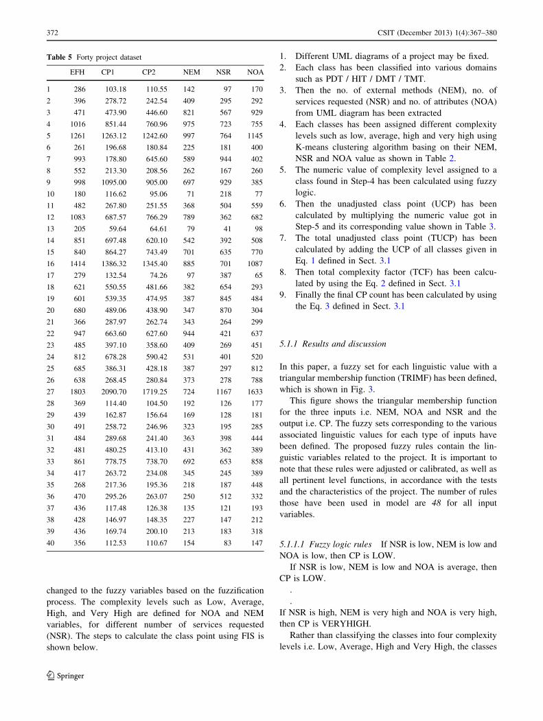
Table 5 Forty project dataset
EFH CP1 CP2 NEM NSR NOA
1 286 103.18 110.55 142 97 170
2 396 278.72 242.54 409 295 292
3 471 473.90 446.60 821 567 929
4 1016 851.44 760.96 975 723 755
5 1261 1263.12 1242.60 997 764 1145
6 261 196.68 180.84 225 181 400
7 993 178.80 645.60 589 944 402
8 552 213.30 208.56 262 167 260
9 998 1095.00 905.00 697 929 385
10 180 116.62 95.06 71 218 77
11 482 267.80 251.55 368 504 559
12 1083 687.57 766.29 789 362 682
13 205 59.64 64.61 79 41 98
14 851 697.48 620.10 542 392 508
15 840 864.27 743.49 701 635 770
16 1414 1386.32 1345.40 885 701 1087
17 279 132.54 74.26 97 387 65
18 621 550.55 481.66 382 654 293
19 601 539.35 474.95 387 845 484
20 680 489.06 438.90 347 870 304
21 366 287.97 262.74 343 264 299
22 947 663.60 627.60 944 421 637
23 485 397.10 358.60 409 269 451
24 812 678.28 590.42 531 401 520
25 685 386.31 428.18 387 297 812
26 638 268.45 280.84 373 278 788
27 1803 2090.70 1719.25 724 1167 1633
28 369 114.40 104.50 192 126 177
29 439 162.87 156.64 169 128 181
30 491 258.72 246.96 323 195 285
31 484 289.68 241.40 363 398 444
32 481 480.25 413.10 431 362 389
33 861 778.75 738.70 692 653 858
34 417 263.72 234.08 345 245 389
35 268 217.36 195.36 218 187 448
36 470 295.26 263.07 250 512 332
37 436 117.48 126.38 135 121 193
38 428 146.97 148.35 227 147 212
39 436 169.74 200.10 213 183 318
40 356 112.53 110.67 154 83 147
372 CSIT (December 2013) 1(4):367–380
123

may be classified into 48 categories according to the
number of transactions per classes. Hence 48 rules gener-
ated to calculate the weight associated with the class. The
MATLAB fuzzy inference system (FIS) was used in the
fuzzy calculations, in addition to the Max-Min composition
operator, the Mamdani implication operator, and the
Maximum operator for aggregation and then the model is
defuzzified.
The fuzzy rule viewer shown in Fig. 4 helps to calculate
the entire implication process from beginning to end.
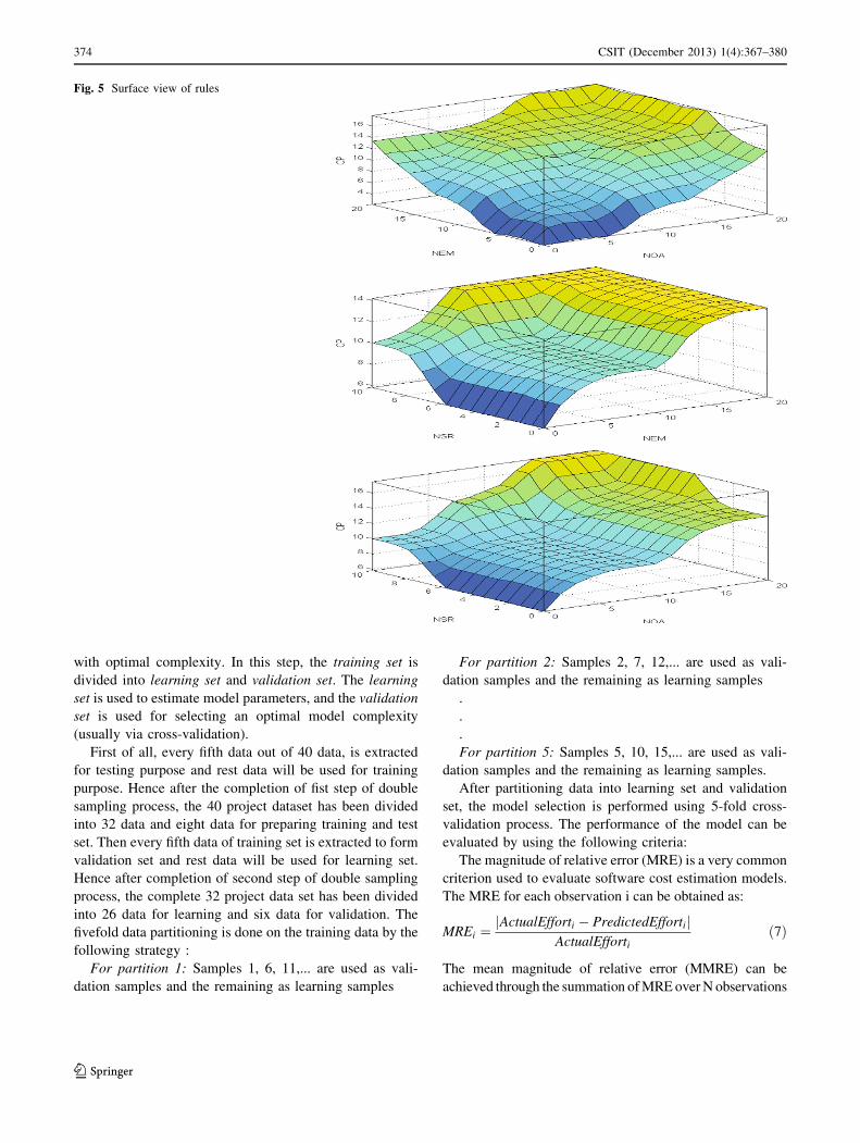
Figure 5 displays the output surface of the FIS used for
class point calculation.
After calculating the final class point values, the data
sets are then being normalized. While implementing the
various adaptive regression techniques for software effort
estimation, the normalized CP2 values have been taken as
input argument to find out the predicted effort. Then the
predicted effort values are compared with the actual effort
values to estimate the accuracy of the different model. The
normalized data set is divided into different subsets using
double sampling procedure. In the first step the normalized
dataset is divided into training set and test set. The training
set is used for learning (model estimation), whereas the test
set is used only for estimating the prediction risk of the
final model. The second step deals with selecting the model
Fig. 4 Fuzzy rule view for class point calculation
0 5 10 15 20
0
0.2
0.4
0.6
0.8
1
NEM
Deg
ree
of m
embe
rshi
p
0 5 10 15 20
0
0.2
0.4
0.6
0.8
1
NOA
Deg
ree
of m
embe
rshi
p
0 2 4 6 8 10
0
0.2
0.4
0.6
0.8
1
NSR
Deg
ree
of m
embe
rshi
p HIGHAVERAGELOW
0 5 10 15 20
0
0.2
0.4
0.6
0.8
1
CP
Deg
ree
of m
embe
rshi
p LOW AVERAGE HIGH VERY HIGH
LOW AVERAGE HIGH VERY HIGH
LOW AVERAGE HIGH VERY HIGH
Fig. 3 Membership function for weight matrix of NEM, NOA, NSR
and CP
Fig. 2 Fuzzy inference system for class point calculation
CSIT (December 2013) 1(4):367–380 373
123
with optimal complexity. In this step, the training set is
divided into learning set and validation set. The learning
set is used to estimate model parameters, and the validation
set is used for selecting an optimal model complexity
(usually via cross-validation).
First of all, every fifth data out of 40 data, is extracted
for testing purpose and rest data will be used for training
purpose. Hence after the completion of fist step of double
sampling process, the 40 project dataset has been divided
into 32 data and eight data for preparing training and test
set. Then every fifth data of training set is extracted to form
validation set and rest data will be used for learning set.
Hence after completion of second step of double sampling
process, the complete 32 project data set has been divided
into 26 data for learning and six data for validation. The
fivefold data partitioning is done on the training data by the
following strategy :
For partition 1: Samples 1, 6, 11,... are used as vali-
dation samples and the remaining as learning samples
For partition 2: Samples 2, 7, 12,... are used as vali-
dation samples and the remaining as learning samples
.
.
.
For partition 5: Samples 5, 10, 15,... are used as vali-
dation samples and the remaining as learning samples.
After partitioning data into learning set and validation
set, the model selection is performed using 5-fold cross-
validation process. The performance of the model can be
evaluated by using the following criteria:
The magnitude of relative error (MRE) is a very common
criterion used to evaluate software cost estimation models.
The MRE for each observation i can be obtained as:
MREi ¼ActualEfforti � PredictedEffortij j
ActualEfforti
ð7Þ
The mean magnitude of relative error (MMRE) can be
achieved through the summation of MRE over N observations
Fig. 5 Surface view of rules
374 CSIT (December 2013) 1(4):367–380
123

MMRE ¼XN
1
MREi ð8Þ
The root mean square error (RMSE) is just the square root
of the mean square error.
RMSE ¼
ffiffiffiffiffiffiffiffiffiffiffiffiffiffiffiffiffiffiffiffiffiffiffiffiffiffiffiffiPNi¼1 yi � �yð Þ2
N
s
ð9Þ
The normalized root mean square (NRMS) can be
calculated by dividing the RMSE value with standard
deviation of the actual effort value for training data set.
NRMS ¼ RMSE
meanðYÞ ð10Þ
where Y is the actual effort for testing data set.
The prediction accuracy (PA) can be calculated as:
PA ¼ 1�PN
i¼1 actual� predictedj jN
! !� 100 ð11Þ
The average of all the folds corresponding NRMSE
value for training and testing set will be considered as the
final NRMSE value of the model. The model producing
lower NRMSE value, will be selected for testing and final
comparison.
5.2 Model design using multi-layer perceptron
This technique uses one parameter. This parameter sets the
number of hidden neurons to be used in a three layer neural
network. The number of neurons used is directly propor-
tional to the training time. The values are typically between
2 and 40, but it can be as high as 1000. While imple-
menting the normalized data set using Multi-Layer Per-
ceptron technique for different number of hidden neurons,
the following results have been obtained.
Table 6 provides minimum NRMSE value obtained
from training set and test set using the multi-layer per-
ceptron technique for each fold for a specific number of
hidden neurons. Hence the final result will be the average
of the NRMSE values for training set and test set. The
proposed model generated using the multi-layer perceptron
technique is plotted based on the training and testing
sample as shown in Fig. 6.
From the above figure, it has been observed that pre-
dicted value is highly correlated with actual data.
5.3 Model design using multivariate adaptive
regression splines
This technique uses two principal tuning parameters. First
parameter is the maximum number of basis functions to use.
This parameter controls the maximum amount of com-
plexity of the model. In most cases, the results are not very
sensitive to this parameter. The range of this parameter is
from 1 to 100. For most problems, this parameter can be set
to a high value (50–100) which results in a good fit.
Second parameter is the amount of penalty given to
complex models. This is an integer, which ranges from 0 to
9 where 0 means a small penalty is given to complex
models and 9 means a large penalty is given. This
parameter is adjusted based on the estimated amount of
noise in the data, and has the largest effect on the results.
For problems with little noise a value less than 5 are sug-
gested. For noisy problems, values larger than 5 can be
used. A good starting value for this parameter is 5.
The model complexity is controlled (in conjunction) by
both the parameters. However, setting the first parameter to a
very large value allows the model complexity to be con-
trolled by just the second parameter. In a simplified way we
can say that, higher the value of second parameter, lower is
the model complexity. While implementing the normalized
data set using MRS technique for number of basis functions
used along with the amount of penalty given to the models,
the following results have been obtained.
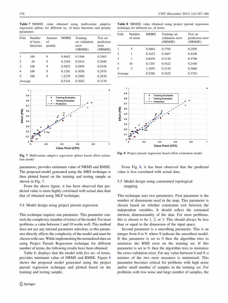
From Table 7, it is clearly visible that the model with
five no. of basis functions and zero amount of penalty
0 0.2 0.4 0.6 0.8 10
0.1
0.2
0.3
0.4
0.5
0.6
0.7
0.8
0.9
1
Class Point (CP2)
Eff
ort
(P
M)
Training ExamplesTesting ExamplesPrediction
Fig. 6 Multi-Layer perceptron based effort estimation model
Table 6 NRMSE value obtained using multi-layer perceptron tech-
nique for different no. of neurons
Fold Number
of hidden
neurons
MMRE Training set
validation error
(NRMSE)
Test set
prediction error
(NRMSE)
1 15 0.4055 0.3282 0.2529
2 25 0.2314 0.3654 0.2606
3 20 0.6468 0.2590 0.5626
4 10 0.1127 0.3117 0.2374
5 30 1.2202 0.2702 0.3501
Average 0.5233 0.3069 0.3327
CSIT (December 2013) 1(4):367–380 375
123
parameters, provides minimum value of NRMS and RMSE.
The proposed model generated using the MRS technique is
then plotted based on the training and testing sample as
shown in Fig. 7.
From the above figure, it has been observed that pre-
dicted value is more highly correlated with actual data than
that of obtained using MLP technique.
5.4 Model design using project pursuit regression
This technique requires one parameter. This parameter con-
trols the complexity (number of terms) of the model. For most
problems, a value between 1 and 10 works well. This method
does not use any internal parameter selection, so this param-
eter directly affects the complexity of the model and must be
chosen with care. While implementing the normalized data set
using Project Pursuit Regression technique for different
number of terms, the following results have been obtained.
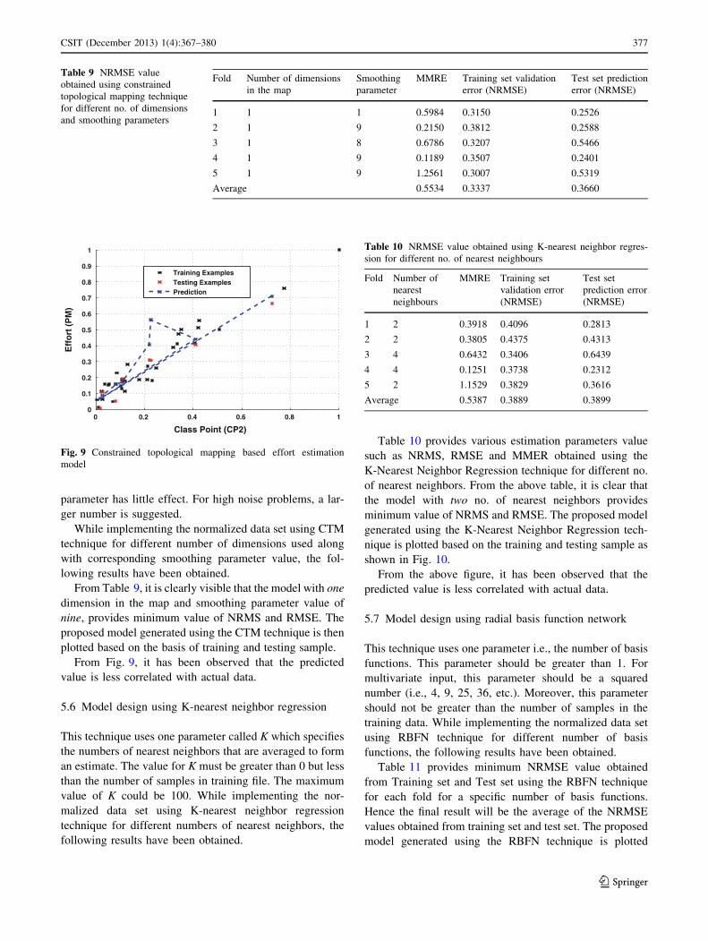
Table 8, displays that the model with five no. of terms,
provides minimum value of NRMS and RMSE. Figure 8
shows the proposed model generated using the project
pursuit regression technique and plotted based on the
training and testing sample.
From Fig. 8, it has been observed that the predicted
value is less correlated with actual data.
5.5 Model design using constrained topological
mapping
This technique uses two parameters. First parameter is the
number of dimensions used in the map. This parameter is
chosen based on whether constraints exit between the
independent variables. It should reflect the estimated
intrinsic dimensionality of the data. For most problems,
this is chosen to be 1, 2, or 3. This should always be less
than or equal to the dimension of the input space.
Second parameter is a smoothing parameter. This is an
integer from 0 to 9, where 9 indicate the smoothest model.
If this parameter is set to 0 then the algorithm tries to
minimize the RMS error on the training set. If this
parameter is set to 9, then the algorithm tries to minimize
the cross-validation error. For any value between 0 and 9, a
mixture of the two error measures is minimized. This
parameter becomes critical for problems with high noise
and/or small number of samples in the training set. For
problems with low noise and large number of samples, the
0 0.2 0.4 0.6 0.8 10
0.1
0.2
0.3
0.4
0.5
0.6
0.7
0.8
0.9
1
Class Point (CP2)
Eff
ort
(P
M)
Training ExamplesTesting ExamplesPrediction
Fig. 7 Multivariate adaptive regression splines based effort estima-
tion model
0 0.2 0.4 0.6 0.8 10
0.1
0.2
0.3
0.4
0.5
0.6
0.7
0.8
0.9
1
Class Point (CP2)
Eff
ort
(P
M)
Training ExamplesTesting ExamplesPrediction
Fig. 8 Project pursuit regression based effort estimation model
Table 7 NRMSE value obtained using multivariate adaptive
regression splines for different no. of basis functions and penalty
parameters
Fold Number
of basis
functions
Amount
of
penalty
MMRE Training
set validation
error
(NRMSE)
Test set
prediction
error
(NRMSE)
1 100 9 0.4042 0.3366 0.2463
2 20 0 0.2384 0.2914 0.2640
3 100 9 0.5852 0.2895 0.5438
4 100 9 0.1201 0.3058 0.2478
5 100 9 1.2239 0.2984 0.2830
Average 0.5144 0.3043 0.3170
Table 8 NRMSE value obtained using project pursuit regression
technique for different no. of terms
Fold Number
of terms
MMRE Training set
validation error
(NRMSE)
Test set
prediction error
(NRMSE)
1 5 0.4064 0.3794 0.2505
2 1 0.3432 0.3667 0.4108
3 1 0.6038 0.3130 0.5798
4 10 0.1201 0.3422 0.2440
5 2 1.1695 0.3110 0.3666
Average 0.5286 0.3425 0.3703
376 CSIT (December 2013) 1(4):367–380
123
parameter has little effect. For high noise problems, a lar-
ger number is suggested.
While implementing the normalized data set using CTM
technique for different number of dimensions used along
with corresponding smoothing parameter value, the fol-
lowing results have been obtained.
From Table 9, it is clearly visible that the model with one
dimension in the map and smoothing parameter value of
nine, provides minimum value of NRMS and RMSE. The
proposed model generated using the CTM technique is then
plotted based on the basis of training and testing sample.
From Fig. 9, it has been observed that the predicted
value is less correlated with actual data.
5.6 Model design using K-nearest neighbor regression
This technique uses one parameter called K which specifies
the numbers of nearest neighbors that are averaged to form
an estimate. The value for K must be greater than 0 but less
than the number of samples in training file. The maximum
value of K could be 100. While implementing the nor-
malized data set using K-nearest neighbor regression
technique for different numbers of nearest neighbors, the
following results have been obtained.
Table 10 provides various estimation parameters value
such as NRMS, RMSE and MMER obtained using the
K-Nearest Neighbor Regression technique for different no.
of nearest neighbors. From the above table, it is clear that
the model with two no. of nearest neighbors provides
minimum value of NRMS and RMSE. The proposed model
generated using the K-Nearest Neighbor Regression tech-
nique is plotted based on the training and testing sample as
shown in Fig. 10.
From the above figure, it has been observed that the
predicted value is less correlated with actual data.
5.7 Model design using radial basis function network
This technique uses one parameter i.e., the number of basis
functions. This parameter should be greater than 1. For
multivariate input, this parameter should be a squared
number (i.e., 4, 9, 25, 36, etc.). Moreover, this parameter
should not be greater than the number of samples in the
training data. While implementing the normalized data set
using RBFN technique for different number of basis
functions, the following results have been obtained.
Table 11 provides minimum NRMSE value obtained
from Training set and Test set using the RBFN technique
for each fold for a specific number of basis functions.
Hence the final result will be the average of the NRMSE
values obtained from training set and test set. The proposed
model generated using the RBFN technique is plotted
0 0.2 0.4 0.6 0.8 10
0.1
0.2
0.3
0.4
0.5
0.6
0.7
0.8
0.9
1
Class Point (CP2)
Eff
ort
(P
M)
Training ExamplesTesting ExamplesPrediction
Fig. 9 Constrained topological mapping based effort estimation
model
Table 10 NRMSE value obtained using K-nearest neighbor regres-
sion for different no. of nearest neighbours
Fold Number of
nearest
neighbours
MMRE Training set
validation error
(NRMSE)
Test set
prediction error
(NRMSE)
1 2 0.3918 0.4096 0.2813
2 2 0.3805 0.4375 0.4313
3 4 0.6432 0.3406 0.6439
4 4 0.1251 0.3738 0.2312
5 2 1.1529 0.3829 0.3616
Average 0.5387 0.3889 0.3899
Table 9 NRMSE value
obtained using constrained
topological mapping technique
for different no. of dimensions
and smoothing parameters
Fold Number of dimensions
in the map
Smoothing
parameter
MMRE Training set validation
error (NRMSE)
Test set prediction
error (NRMSE)
1 1 1 0.5984 0.3150 0.2526
2 1 9 0.2150 0.3812 0.2588
3 1 8 0.6786 0.3207 0.5466
4 1 9 0.1189 0.3507 0.2401
5 1 9 1.2561 0.3007 0.5319
Average 0.5534 0.3337 0.3660
CSIT (December 2013) 1(4):367–380 377
123

based on the training and testing sample as shown in
Fig. 11.
From the above figure, it has been observed that the
predicted value is highly correlated with actual data, but
less correlation than that of obtained using MRS technique.
5.8 Comparison
On the basis of results obtained, the estimated effort value
using the six adaptive methods for regression are com-
pared. The results show that effort estimation using MRS
gives better values of NRMSE than those obtained using
other five methods.
Figure 12 shows the comparison between MMRE values
obtained using six adaptive regression methods.
Figure 13 shows the comparison between validation
error obtained using six adaptive regression methods.
Figure 14 shows the comparison between prediction
error obtained using six adaptive regression methods.
0 0.2 0.4 0.6 0.8 10
0.1
0.2
0.3
0.4
0.5
0.6
0.7
0.8
0.9
1
Class Point (CP2)
Eff
ort
(P
M)
Training ExamplesTesting ExamplesPrediction
Fig. 10 K-nearest neighbor regression based effort estimation model
0 0.2 0.4 0.6 0.8 10
0.1
0.2
0.3
0.4
0.5
0.6
0.7
0.8
0.9
1
Class Point (CP2)
Eff
ort
(P
M)
Training ExamplesTesting ExamplesPrediction
Fig. 11 Radial basis function network based effort estimation model
1 2 3 4 50
0.2
0.4
0.6
0.8
1
1.2
1.4
Fold Number
MM
RE
MLP
MRS
PPR
CTM
KNN
RBFN
Fig. 12 Comparison of MMRE values obtained using six adaptive
methods for regression
1 2 3 4 50
0.05
0.1
0.15
0.2
0.25
0.3
0.35
0.4
0.45
0.5
Fold Number
Val
idat
ion
Err
or
MLP
MRS
PPR
CTM
KNN
RBFN
Fig. 13 Comparison of validation error obtained using six adaptive
methods for regression
Table 11 NRMSE value obtained using radial basis function net-
work technique based on no. of basis functions
Fold Number
of basis
functions
MMRE Training set
validation error
(NRMSE)
Test set
prediction error
(NRMSE)
1 2 0.3961 0.4525 0.2495
2 2 0.2282 0.3985 0.3158
3 2 0.6601 0.3546 0.5566
4 2 0.1208 0.3817 0.2438
5 2 1.2207 0.3411 0.3063
Average 0.5252 0.3857 0.3344
378 CSIT (December 2013) 1(4):367–380
123

Figure 15 shows the comparison of average error values
obtained from training set (validation error) and test set
(prediction error) for six adaptive methods for regression
techniques.
When using the NRMSE, MMRE and prediction accu-
racy in evaluation, good results are implied by lower values
of NRMSE, MMRE and higher values of prediction accu-
racy. Table 12 displays the final comparison of NRMSE,
MMRE and prediction accuracy value for six adaptive
regression methods. From the table, it is clear that the effort
estimation using MRS method gives least NRMSE, MMRE
and high prediction accuracy value than other five tech-
niques. Similarly, a comparison has been made between the
obtained results with the work mentioned in the related work
section. By analyzing results, it can be concluded that the
prediction accuracy obtained by Costagliola et al. [10],
Zhou and Liu [28] and Kanmani et al. [19] is 83, 83 and
87 % respectively; where as the proposed techniques shows
significant improvement in the accuracy values as shown in
Table 12. Hence, it can be concluded that the proposed
approaches outperform the techniques mentioned in the
related work section.
6 Conclusion and future work
Several approaches have already been defined in literature
for software effort estimation. But the CPA is one of the
different cost estimation models that has been widely used
because it is simple, fast and accurate to a certain degree.
Fuzzy-logic technique is further used to find out the com-
plexity level of the class and to calculate optimized class
point. Then the calculated class point values are being
normalized and used to optimize the effort estimation
result. The optimal values are obtained by implementing
six different types of adaptive methods of regression
techniques such as ANN, MRS, PPR, CTM, KNN and
RBFN using normalized class point value. Finally the
generated minimum results of different techniques have
been compared to estimate their performance accuracy.
Result shows that MRS based effort estimation model gives
less value of NRMSE, MMRE and higher value of
1 2 3 4 50
0.1
0.2
0.3
0.4
0.5
0.6
0.7
Fold Number
Pre
dic
tio
n E
rro
rMLP
MRS
PPR
CTM
KNN
RBFN
Fig. 14 Comparison of prediction error obtained using six adaptive
methods for regression
MLP MRS PPR CTM KNN RBFN0
0.1
0.2
0.3
0.4
0.5
0.6
0.7
Models
Ave
rag
e E
rro
r
MMREAVG
VEAVG
PEAVG
Fig. 15 Comparison of average error values obtained from training
and test set using six adaptive methods for regression
Table 12 Comparison of NRMSE, MMRE and prediction accuracy
values between six adaptive methods for regression
Average
validation
error
(NRMSE)
Average
prediction
error
(NRMSE)
Average
MMRE
Prediction
accuracy (in
percentage)
Multi-layer
perceptron
0.3069 0.3327 0.5233 94.8185
Multivariate
adaptive
regression
splines
0.3043 0.3170 0.5144 95.0639
Projection
pursuit
regression
0.3425 0.3703 0.5286 94.0546
Constrained
topological
mapping
0.3337 0.3660 0.5534 94.5322
K nearest
neighbor
regression
0.3889 0.3899 0.5387 93.8137
Radial basis
function
network
0.3857 0.3344 0.5252 94.7539
CSIT (December 2013) 1(4):367–380 379
123

prediction accuracy. Hence it can be concluded that the
effort estimation using MRS model will provide more
accurate results than other five techniques. The computa-
tions for above procedure have been implemented and
membership functions generated using MATLAB. This
approach can also be extended by using some other tech-
niques such as Random Forest and Gradient Boosted Trees.
References
1. Albrecht AJ Measuring application development productivity. In
Proceedings of the Joint SHARE/GUIDE/IBM Application
Development Symposium, volume 10, pages 83–92. SHARE Inc.
and GUIDE International Corp. Monterey, CA, 19;79
2. Attarzadeh I, Ow S (2010) Soft computing approach for software
cost estimation. Int J Software Eng, IJSE 3(1):1–10
3. Bataineh K, Naji M, Saqer M (2011) A comparison study between
various fuzzy clustering algorithms. Editorial Board, 5(4):335
4. Bors A (2001) Introduction of the radial basis function (rbf)
networks. In Online symposium for electronics engineers, volume
1, pp 1–7
5. Braga PL, Oliveira AL, Meira SR (2008) A ga-based feature
selection and parameters optimization for support vector regression
applied to software effort estimation. In Proceedings of the 2008
ACM symposium on Applied computing, pp 1788–1792. ACM
6. Carbone M, Santucci G (2002) Fast&&serious: a UML based
metric for effort estimation. In: Proceedings of the 6th ECOOP
workshop on quantitative approaches in object-oriented software
engineering (QAOOSE’02), pp 313–322
7. Cherkassky V, Gehring D, Mulier F (1996) Comparison of
adaptive methods for function estimation from samples. IEEE
Trans Neural Netw 7(4):969–984
8. Cherkassky V, Lari-Najafi H (1991) Constrained topological
mapping for nonparametric regression analysis. Neural Netw
4(1):27–40
9. Cherkassky V, Mulier FM (2007) Learning from data: concepts,
theory, and methods. Wiley-IEEE Press, New Jersey
10. Costagliola G, Ferrucci F, Tortora G, Vitiello G (2005) Class
point: an approach for the size estimation of object-oriented
systems. IEEE Trans Soft Eng 31(1):52–74
11. Costagliola G, Ferrucci F, Tortora G, Vitiello G (1998) Towards
a software size metrics for object-oriented systems. Proc. AQUIS
98:121–126
12. Devroye L (1978) The uniform convergence of nearest neighbor
regression function estimators and their application in optimiza-
tion. IEEE Trans Inf Theory 24(2):142–151
13. Drucker H, Burges CJ, Kaufman L, Smola A, Vapnik V (1997)
Support vector regression machines.In Mozer M.C., Jordan M.I.,
and Petsche T. (eds) Advances in neural information processing
systems. MIT Press, Cambridge, pp 155–161
14. Friedman JH (1991) Multivariate adaptive regression splines.
Ann Stat 19:1–67
15. Friedman JH, Stuetzle W (1981) Projection pursuit regression.
J Am Stat Assoc 76(376):817–823
16. Heemstra F, Kusters R (1991) Function point analysis: evaluation
of a software cost estimation model. Eur J Inf Syst 1(4):229–237
17. Idri A, Abran A, Mbarki S (2006) An experiment on the design of
radial basis function neural networks for software cost estimation.
In Information and Communication Technologies, 2006. ICT-
TA’06. 2nd, vol 1, IEEE, pp 1612–1617.
18. Kanmani S, Kathiravan J, Kumar SS, Shanmugam M (2008)
Class point based effort estimation of OO systems using fuzzy
subtractive clustering and ANNs. In Proceedings of the 1st India
software engineering conference, ISEC ’08, ACM, pp 141–142,
New York, NY, USA, 2008.
19. Kanmani S, Kathiravan, J, Senthil Kumar S, Shanmugam M
(2007) Neural network based effort estimation using class points
for OO systems. In Computing: Theory and Applications, 2007.
ICCTA’07. International Conference on IEEE, pp 261–266
20. Kim S, Lively W, Simmons D (2006) An effort estimation by
UML points in early stage of software development. In: Pro-
ceedings of the international conference on software engineering
research and practice, pp 415–421
21. Klair AS, Kaur RP (2012) Software effort estimation using SVM
and KNN. In international conference on computer graphics,
simulation and modeling (ICGSM2012), pp 146–147
22. Matson JE, Barrett BE, Mellichamp JM (1994) Software devel-
opment cost estimation using function points. IEEE Trans Soft
Eng 20(4):275–287
23. Oliveira AL (2006) Estimation of software project effort with
support vector regression. Neurocomputing 69(13):1749–1753
24. Panchapakesan C, Palaniswami M, Ralph D, Manzie C (2002)
Effects of moving the center’s in an rbf network. IEEE Trans
Neural Netw 13(6):1299–1307
25. S Moertini V (2008) Introduction to five data clustering algo-
rithms. INTEGRAL Majalah Ilmiah Matematika dan Ilmu
Pengetahuan Alam 7(2)
26. Sarimveis H, Alexandridis A, Bafas G (2003) A fast training
algorithm for rbf networks based on subtractive clustering.
Neurocomputing 51:501–505
27. Smola AJ, Scholkopf B (2004) A tutorial on support vector
regression. Stat Comput 14(3):199–222
28. Zhou W, Liu Q (2010) Extended class point approach of size
estimation for OO product. In 2nd international conference on
computer engineering and technology (ICCET), 2010, vol 4,
IEEE pp 117–122
380 CSIT (December 2013) 1(4):367–380
123


![Chapter 3: Fuzzy Rules & Fuzzy Reasoning513].pdf · CH. 3: Fuzzy rules & fuzzy reasoning 1 Chapter 3: Fuzzy Rules & Fuzzy Reasoning ... Application of the extension principle to fuzzy](https://img.dokumen.tips/doc/110x75/5b3ed7b37f8b9a3a138b5aa0/chapter-3-fuzzy-rules-fuzzy-513pdf-ch-3-fuzzy-rules-fuzzy-reasoning.jpg)