Portfolio Optimization under Expected Shortfall: Contour Maps of Estimation ErrorFabio Caccioli

Imre Kondor

Gábor Papp

SRC Discussion Paper No 49

November 2015

ISSN 2054-538X

Abstract The contour maps of the error of historical resp. parametric estimates for large random portfolios optimized under the risk measure Expected Shortfall (ES) are constructed. Similar maps for the sensitivity of the portfolio weights to small changes in the returns as well as the VaR of the ES-optimized portfolio are also presented, along with results for the distribution of portfolio weights over the random samples and for the out-of-sample and in-the-sample estimates for ES. The contour maps allow one to quantitatively determine the sample size (the length of the time series) required by the optimization for a given number of different assets in the portfolio, at a given confidence level and a given level of relative estimation error. The necessary sample sizes invariably turn out to be unrealistically large for any reasonable choice of the number of assets and the confi dence level. These results are obtained via analytical calculations based on methods borrowed from the statistical physics of random systems, supported by numerical simulations. This paper is published as part of the Systemic Risk Centre’s Discussion Paper Series. The support of the Economic and Social Research Council (ESRC) in funding the SRC is gratefully acknowledged [grant number ES/K002309/1]. Fabio Caccioli, Department of Computer Science, University College London and Systemic Risk Centre, London School of Economics and Political Science Imre Kondor, Parmenides Foundation, Pullach, Germany and Department of Investment and Corporate Finance, Corvinus University of Budapest, Budapest, Hungary Gárbo Papp, Eötvös Loránd University, Institute for Physics, Budapest, Hungary Published by Systemic Risk Centre The London School of Economics and Political Science Houghton Street London WC2A 2AE All rights reserved. No part of this publication may be reproduced, stored in a retrieval system or transmitted in any form or by any means without the prior permission in writing of the publisher nor be issued to the public or circulated in any form other than that in which it is published. Requests for permission to reproduce any article or part of the Working Paper should be sent to the editor at the above address. © Fabio Caccioli, Imre Kondor, and Gárbo Papp, submitted 2015

Portfolio Optimization under Expected Shortfall: Contour

Maps of Estimation Error

Fabio Caccioli1,2, Imre Kondor3,4 and Gabor Papp5

1- University College London, Department of Computer Science,London, WC1E 6BT, UK

2- Systemic Risk Centre, London School of Economics and Political Sciences, London, UK3-Parmenides Foundation, Pullach, Germany

4- Department of Investment and Corporate Finance, Corvinus University of Budapest,Budapest, Hungary

5- Eotvos Lorand University, Institute for Physics, Budapest, Hungary

Abstract

The contour maps of the error of historical resp. parametric estimates for largerandom portfolios optimized under the risk measure Expected Shortfall (ES) are con-structed. Similar maps for the sensitivity of the portfolio weights to small changes inthe returns as well as the VaR of the ES-optimized portfolio are also presented, alongwith results for the distribution of portfolio weights over the random samples and forthe out-of-sample and in-the-sample estimates for ES. The contour maps allow one toquantitatively determine the sample size (the length of the time series) required by theoptimization for a given number of different assets in the portfolio, at a given confi-dence level and a given level of relative estimation error. The necessary sample sizesinvariably turn out to be unrealistically large for any reasonable choice of the numberof assets and the confidence level. These results are obtained via analytical calculationsbased on methods borrowed from the statistical physics of random systems, supportedby numerical simulations.

1 Introduction

Risk measurement and portfolio optimization are two complementary aspects of portfoliotheory. Both assume that the future will statistically resemble the past, but while riskmeasurement is trying to forecast the risk of an existing portfolio, optimization is attempt-ing to choose the composition of the portfolio in such a way as to minimize risk at a givenlevel of expected return (or maximize return at a given level of risk). In the case of largeinstitutional portfolios both tasks require a large number of input data, i.e. large samples

1

of observed returns. The inherent difficulty both of risk measurement and optimization liesin the fact that these large sample sizes are typically hard if not impossible to achieve inpractice. On the portfolio selection side in particular, the difficulty is further aggravatedby the fact that here the sample size must be large not only compared to one, but alsoto the size (measured in the number of different assets) of the portfolio. In order to havesamples exceeding the dimensions of large institutional portfolios with numbers of assetsin the hundreds or thousands, one would need either a high sampling frequency, or a longlook-back period, and preferably both. The length of the look-back period is limited byconsiderations of lack of stationarity: some of the assets in the portfolio may be sharesof firms that have not been in existence for a very long time, the economic and monetaryenvironment may have changed, new regulatory constraints may have been introduced, etc.As for the sampling frequency, it is limited by the frequency at which portfolios can practi-cally be rebalanced, so we assume in the following that the portfolio manager uses such lowfrequency (weekly or rather monthly) data. This means that the sample size (the length ofthe time series T ) is always limited, while the dimension N of institutional portfolios (thenumber of different assets) is typically very large, and the condition N/T � 1 necessaryfor reliable and stable estimates is almost always violated in practice. In this paper we willconsider situations where N and T are both very large, but their ratio is finite.

Both risk measurement and optimization require a metric, a measure of risk. In Markowitz’soriginal theory of portfolio optimization [1] the risk measure was chosen to be the volatilityof the return data, identified with the variance of the observed time series. If one mea-sures risk in terms of the variance, this equally penalizes large negative as well as positivefluctuations. The symmetric treatment of loss and gain was considered unjustified fromthe point of view of the investor, therefore the idea of downside risk measures, focusingsolely on losses, was introduced very early, already by Markowitz [2], in the form of thesemivariance. A few decades later, in the aftermath of the meltdown on Black Monday inOctober 1987, and the collapse of the US savings and loan industry in the late 80’s andearly 90’s, it was realized that the really lethal danger lurked in the far tail of the loss dis-tribution and that the probability of such catastrophic events was much higher than whatcould be estimated on the basis of the normal distribution. Value at Risk (VaR) startedto sporadically appear around the end of the 80’s as an attempt at grasping this tail risk.It was adopted as the metric in the daily risk reports at J.P. Morgan, later widely spreadby their RiskMetrics methodology [3] that for a certain period became a sort of industrystandard. VaR’s status was further elevated when it became adopted as the “official” riskmeasure by international regulation in 1996 [4].

Value at Risk (VaR) is a high quantile of the profit and loss distribution, the threshold theportfolio’s loss will not exceed with probability α. In practice, the typical values of thisconfidence level were chosen to be 0.90, 0.95, or 0.99.

In spite of its undeniable merits, VaR came under criticism very soon for its lack of sub-

2

additivity, which violated the principle of diversification, and also for its failure to sayanything about the behaviour of the distribution beyond the VaR quantile. By an ax-iomatic approach to the problem of risk measures, Artzner et al. [5] introduced the conceptof coherent measures that are free of these shortcomings by construction. The simplestrepresentative of coherent measures is Expected Shortfall (ES), the average risk above ahigh quantile that can be chosen to be equal to the VaR threshold. For this reason ES isalso called conditional VaR or CVaR.

As a conditional average, ES is sensitive not only to the total mass of fluctuations abovethe quantile, but also to their distribution. This, and its coherence proved by Pflug [6]and Acerbi and Tasche [7, 8] has made it popular among theoreticians, but increasinglyalso among practitioners. Recently, it has also been embraced by regulation [9, 10] thatenvisages a confidence level of 0.975 for ES.

Today VaR and ES are the two most frequently used risk measures. It is therefore importantto investigate their statistical properties, especially in the typical high-dimensional setting.The lack of sufficient data which, for large portfolios, can be very serious for any riskmeasure is particularly grave in the case of downside risk measures (such as VaR and ES)that discard most of the observed data except those above the high quantile.

A comprehensive recent treatment of the risk measurement aspect of the problem is due toDanielsson and Zhou [11]. Our purpose here is to look into the complementary problem:that of portfolio selection. If we knew the true probability distribution of returns, it wouldbe straightforward to determine the optimal composition of the portfolio (the optimalportfolio weights) and calculate the true value of Expected Shortfall. The true distributionof returns is, however, unknown. What we may have in practice is only a finite sample,and the optimal weights and ES have to be estimated on the basis of this information. Theresulting weights and ES will deviate from their “true” values (that would be obtained inan infinitely large stationary sample), and the deviation can be expected to be the strongerthe shorter the length T of the sample and the larger the dimension N of the portfolio. Inaddition, in a different sample we would obtain a different estimate: there is a distributionof ES and of the optimal weights over the samples.

How can one cope with the estimation error arising from this relative scarcity of data? Inactual practice, where one really has to live with a single sample of limited size, one may usecross-validation or bootstrap [12]. In the present theoretical work, we choose an alternativeprocedure to mimic historical estimation: Instead of the unknown underlying process, weconsider a simple, easily manageable one, such as a multivariate Gaussian process, wherethe true ES is easy to obtain, thereby creating a firm basis for comparison. Then wecalculate ES for a large number of random samples of length T drawn from this underlyingdistribution, average ES over these random samples and finally compare this average to itstrue value. This excercise will give us an idea about how large the estimation error can befor a given dimension N and sample size T , and we may expect that the optimization of

3

portfolios under ES with a non-stationary and fat tailed real-life process will suffer froman even more serious estimation error than its Gaussian counterpart. In other words, weexpect that the estimation error for a stationary Gaussian underlying process is a lowerbound for the estimation error for real-life processes.

This program can certainly be carried out by numerical simulations. To obtain analyticalresults for ES optimization is, however, nontrivial and we are not aware of any analyticalapproach using standard methods of probability theory or statistics that could be applied tothis problem. However, methods borrowed from the theory of random systems, in particularthe replica method [13], do offer the necessary tools in the special case of a Gaussianunderlying process, and these are the methods we are going to apply here. For the sakeof simplicity, we will also assume that the returns are independent, identically distributednormal variables, although the assumptions of independence and identical distributioncould be relaxed and the calculation could still be carried through without essentiallychanging the conclusions. We will briefly discuss the case of normal variables with anarbitrary (but invertible) covariance matrix later in the paper.

The Gaussian assumption is more serious: if we drop it, we are no longer able to performthe calculations analytically. Numerical simulations remain feasible, however, and we willcarry out simulations for the case of independent Student-distributed returns (with ν = 3degrees of freedom, asymptotically falling off like x−4), in order to see how much differencethe fat tailed character of this distribution makes in the estimation error. (We will alsoconsider a Student distribution with ν = 10 to show how the numerical results approachthe Gaussian case.) As expected, the large fluctuations at the tail result in a deteriorationof the estimated ES. This supports our conjecture that the estimation error found in thecase of normally distributed returns is a lower bound to the estimation error for other, morerealistic distributions, and for that reason the present exercise has a message for portfoliooptimization in general.

The analytical technique we are going to apply enables us to calculate the relative error ofES and the distribution of optimal portfolio weights averaged over the random Gaussiansamples, but does not provide information (at least not without a great deal of additionaleffort) about how strongly these quantities fluctuate from sample to sample. In the limitof large portfolio sizes the distribution of estimated Expected Shortfall and its error can beexpected to become sharp, with ES and the estimation error becoming independent of thesamples1. In order to acquire information about the distribution of these estimates overthe samples, we will resort to numerical simulations again. We find that the distributionof the estimated ES over the samples is becoming reasonably sharp already for N ’s in therange of a few hundred, so the sample average can give us a good idea about the estimationerror. In the vicinity of some special, critical points, however, the average estimation error

1For a rigorous mathematical proof of this “self-averaging” in the case of related models of statisticalphysics see [14,15]

4

can grow beyond any bound, and there its fluctuations also diverge.

As we have already mentioned, the lack of sufficient information leads to large errors inthe estimation of optimal weights and overall portfolio risk under any risk measure. In thecase of e.g. the variance as risk measure, it is well known that the sample size T must bemuch larger than the dimension N of the portfolio, if we wish to obtain a good estimateof the risk. For N and T both large, the relevant combination of these parameters turnsout to be the aspect ratio r = N/T . For N/T � 1, we will have a good quality estimate.Upon approaching a critical value, which for the optimization of variance is N/T = 1, thesample to sample fluctuations become stronger and stronger, until at N/T = 1 the averagerelative estimation error becomes infinitely large [16, 17]. At this point the covariancematrix ceases to be positive definite, and the optimization task becomes meaningless. Wecan regard N/T = 1 as a critical point at which a phase transition is taking place.

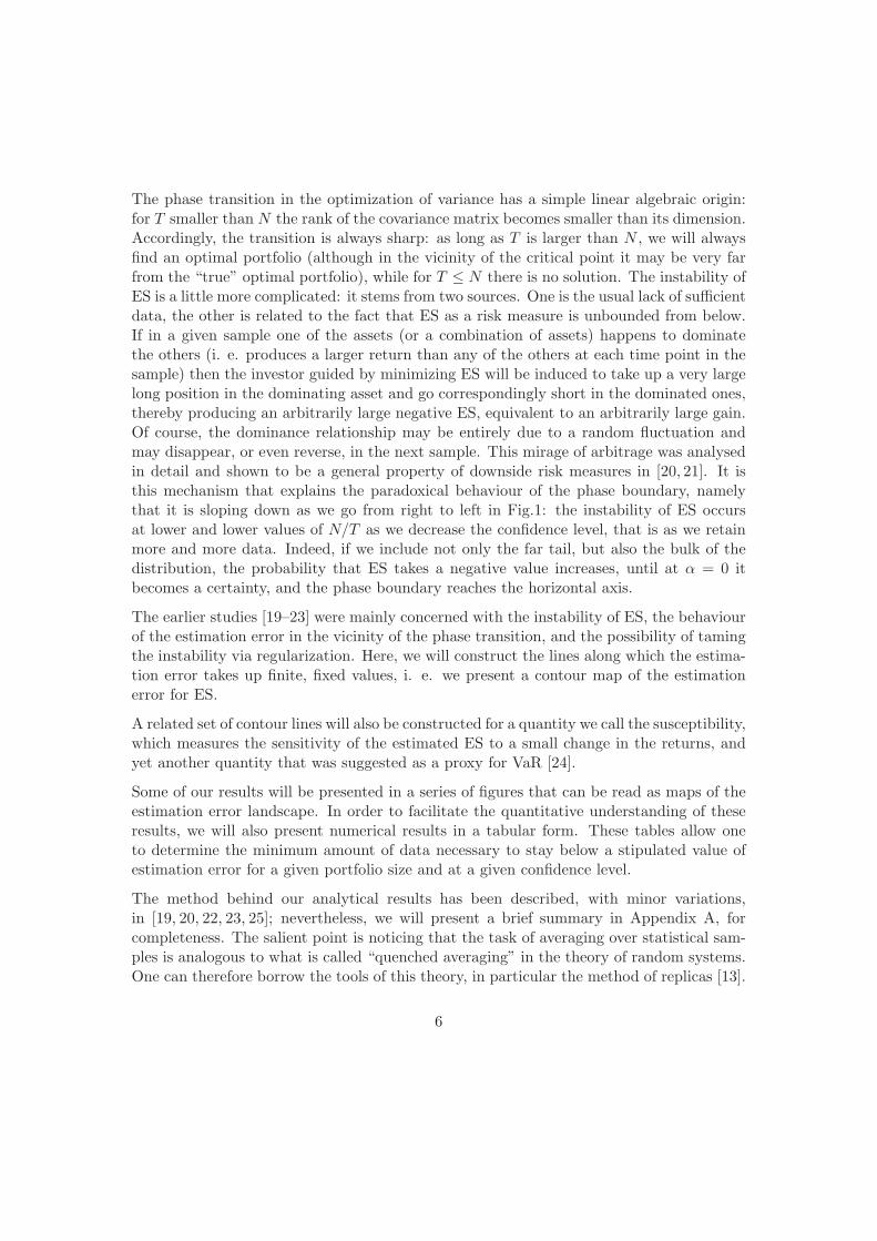
Similar critical phenomena appear also for other risk measures. In the case of ES we haveanother control parameter, the confidence limit α, in addition to the aspect ratio N/T .There is a different critical value of N/T for each α between 0 and 1, thus we have a criticalline on the α – N/T plane. This critical line separates the region where the optimizationcan be carried out from the region where it is not feasible. We will refer to this line asthe phase boundary. In the special case of i.i.d. normal underlying returns, the phaseboundary of ES was partially traced out by numerical simulations in [18] and determinedby analytical methods in [19]. It is displayed in Fig.1.

0.0 0.2 0.4 0.6 0.8 1.0

0.0

0.1

0.2

0.3

0.4

0.5

α

r

Figure 1: The phase boundary of ES for i.i.d. normal underlying returns. In the region below the phaseboundary the optimization of ES is feasible and the estimation error is finite. Approaching the phaseboundary from below, the estimation error diverges, and above the line optimization is no longer feasible.

5

The phase transition in the optimization of variance has a simple linear algebraic origin:for T smaller than N the rank of the covariance matrix becomes smaller than its dimension.Accordingly, the transition is always sharp: as long as T is larger than N , we will alwaysfind an optimal portfolio (although in the vicinity of the critical point it may be very farfrom the “true” optimal portfolio), while for T ≤ N there is no solution. The instability ofES is a little more complicated: it stems from two sources. One is the usual lack of sufficientdata, the other is related to the fact that ES as a risk measure is unbounded from below.If in a given sample one of the assets (or a combination of assets) happens to dominatethe others (i. e. produces a larger return than any of the others at each time point in thesample) then the investor guided by minimizing ES will be induced to take up a very largelong position in the dominating asset and go correspondingly short in the dominated ones,thereby producing an arbitrarily large negative ES, equivalent to an arbitrarily large gain.Of course, the dominance relationship may be entirely due to a random fluctuation andmay disappear, or even reverse, in the next sample. This mirage of arbitrage was analysedin detail and shown to be a general property of downside risk measures in [20, 21]. It isthis mechanism that explains the paradoxical behaviour of the phase boundary, namelythat it is sloping down as we go from right to left in Fig.1: the instability of ES occursat lower and lower values of N/T as we decrease the confidence level, that is as we retainmore and more data. Indeed, if we include not only the far tail, but also the bulk of thedistribution, the probability that ES takes a negative value increases, until at α = 0 itbecomes a certainty, and the phase boundary reaches the horizontal axis.

The earlier studies [19–23] were mainly concerned with the instability of ES, the behaviourof the estimation error in the vicinity of the phase transition, and the possibility of tamingthe instability via regularization. Here, we will construct the lines along which the estima-tion error takes up finite, fixed values, i. e. we present a contour map of the estimationerror for ES.

A related set of contour lines will also be constructed for a quantity we call the susceptibility,which measures the sensitivity of the estimated ES to a small change in the returns, andyet another quantity that was suggested as a proxy for VaR [24].

Some of our results will be presented in a series of figures that can be read as maps of theestimation error landscape. In order to facilitate the quantitative understanding of theseresults, we will also present numerical results in a tabular form. These tables allow oneto determine the minimum amount of data necessary to stay below a stipulated value ofestimation error for a given portfolio size and at a given confidence level.

The method behind our analytical results has been described, with minor variations,in [19, 20, 22, 23, 25]; nevertheless, we will present a brief summary in Appendix A, forcompleteness. The salient point is noticing that the task of averaging over statistical sam-ples is analogous to what is called “quenched averaging” in the theory of random systems.One can therefore borrow the tools of this theory, in particular the method of replicas [13].

6

The replica method is very powerful and is capable of delivering results which have notbeen accessible through any other analytical approach so far. To position our work vis-a-visthe extended literature on the estimation error problem in portfolio selection, we note thatmost of this literature is based on the analysis of finite (empirical or synthetic) samples,combined with various noise reduction methods ranging from Bayesian [26–28], throughshrinkage [29–32], lasso [33], random matrix [34–37], and a number of other techniques.The set of purely theoretical papers that deal with the problem with the standard tools ofprobability theory and statistics is much smaller and concerned with the estimation errorin mean-variance optimization [38–40]. A relatively recent review of the field of portfoliooptimization is [41]. Analytical results on the estimation error problem of risk measuresother than the variance do not exist beyond the few papers [19, 20, 22, 23, 25] that appliedreplicas in the present context.

It should be noted, however, that the method of replicas has a shortcoming in that at acertain point of the derivation one has to analytically continue the formulae from the setof natural numbers to the reals, and the uniqueness of this continuation is very hard toprove. In a number of analogous problems in statistical physics a rigorous proof couldbe constructed even in the much more complicated case of a non-convex cost function[42]. Although we cannot offer such a rigorous proof here, it is hard to imagine how themethod could lead one astray when the cost function is convex and has a single minimum.Nevertheless, in the lack of a rigorous mathematical proof we felt compelled to always checkthe results of replicas by numerical simulations, and always found complete agreement.

The main conclusion this study has led us to is that the error both in the composition ofthe estimated optimal portfolio and its resulting ES is very large unless the aspect ratioN/T is very small. Qualitatively, this is a foregone conclusion. The novelty is the setof quantitative results showing exactly how large the sample sizes should be to achieve areasonably low level of estimation error, and how much these sample sizes exceed anythingthat can be realistically hoped to be available in the industry. It also turns out thatincluding more data (setting a lower confidence level) would not help: the contour lines ofrelative error in the acceptable range of, say 5%, are rather flat. What all this means isthat for typical parameter values N,T the estimation error is so large as to make portfoliooptimization illusory.

Everything we said so far concerns historical estimates. One may expect that parametricestimates suffer less from the estimation error. This is indeed so - though the differenceis less than what one might have hoped for. In [20] we derived the phase boundary forparametric VaR and ES by the technique of replicas again and found that the critical line ofparametric ES lies above that of the historical estimate, so it moves in the good direction. Inthis paper we extend those results and construct the countour lines of parametric estimatesalong which ES is a given finite constant. We find that the parametric estimates are indeedless demanding than the historical ones, which is natural, given that with the choice of

7

the target distribution we project a lot of information into the estimate. The gain is,however, far from sufficient to allow even the parametric estimates to produce acceptablylow estimation errors for realistic portfolio and sample sizes - and this despite the factthat we were fitting a Gaussian distribution to finite samples generated by a Gaussian. Inreal life one should fit a fat tailed distribution to empirical data, a task as fraught withuncertainty as estimating a high quantile or a conditional average above it.

Finally, a word on regularization. The standard way of dealing with high-dimensionalstatistics is to use regularization [43], which in the given context would mean imposing apenalty on the large excursions of the portfolio weights, thereby reducing the estimationerror. We studied the effect of regularization on the estimation of ES in [22,23,44]. Here, werefrain from considering the effect of possible regularizers, because our primary purpose isto show up how serious the raw estimation error problem is. We plan to return to the studyof various regularizers in a future publication where we wish to assess the bias-estimationerror tradeoff in richer data generating processes than the i.i.d. Gaussian considered here.

The plan of the paper is as follows: In Sec. 2 we lay out the task of optimizing ES, fixnotation and recall how [24] reduced this problem to linear programming. In Sec. 3 wedefine the various quantities characterizing the estimation error: the in-the-sample andout-of-sample estimates of ES, the relative estimation error, the sample average of theestimated distribution of portfolio weights, and the susceptibility. These are the quantitieswe set out to calculate by the method of replicas. The explanation of the replica methodis relegated to Appendix A, where the generating functional whose minimum will give theanswer to our optimization problem is derived as a function of six variables, the so calledorder parameters. The first order conditions determining the order parameters are writtenup in Sec. 4, where also the various measures of estimation error defined in the previoussection are identified in the replica language. The main features of the solutions of the firstorder conditions are explained in Sec. 5. The solutions themselves are mainly obtained bynumerical computation, in a few special cases one can gain insight into the structure of theequations by analytical calculation, some details of which are presented in Appendix B.The central results for historical estimates are presented in Sec. 6 mainly in graphical, butalso in tabular form. Section 7 discusses the problem of parametric estimates, and makesa comparison with the historical ones. The bulk of the paper is dealing with the simplestpossible realization of the estimation error problem: an i.i.d. normal underlying process,estimation of the global minimum portfolio (omitting the constraint of the expected return),etc. In Sec. 8 we consider each of these simplifications in turn, and look into whether theycould modify the main message of the paper. Correlated and non identically distributed butstill Gaussian underlying fluctuations could be easily accommodated, as could the inclusionof the constraint on expected return. Where numerical simulations remain the only toolare the problems of fat tailed distributions, and the error bars on the average estimationerror. These simulations do not pose a problem in principle, but are very computationintensive, so we just present a few illustrative examples. The conclusion of the study of all

8

these possible extensions is that they can modify some of the details of the results obtainedin the simplest setup, but do not change the main message of the paper in any meaningfulway. Finally, in Sec.9 we summarize the most important results, and indicate the directionsalong which the present work can be continued.

2 The optimization of ES

The simple portfolios we consider here are linear combinations of N securities, with returnsxi, i = 1, 2, ..., N and weights wi:

X =

N∑i=1

wixi (1)

The weights will be normalized such that their sum is N , instead of the customary 1. Themotivation for choosing this normalization is that we wish to have weights of order unity,rather than 1/N , in the limit N → ∞:

N∑i=1

wi = N. (2)

Apart from this budget constraint the weights will not be subject to any other condition. Inparticular, they can take any real value, that is we are allowing unlimited short positions.Admittedly, this is rather unrealistic: Depending on the type of institutional investor, shortpositions may be limited or even excluded by legal and/or liquidity constraints. However,when they are present, even if subject to limits, they greatly contribute to the instabilityof ES. A ban on short positions would act as a hard l1 regularizer and would eliminate theinstability [23], at least for what concerns the magnitude of ES. (Large fluctuations in theoptimal weights may remain even after regularization.) A detailed discussion of the effectsof various regularizers will be left for a separate publication, here we focus on the simplest,unregularized case and wish to display the estimation error stemming from the intrinsicinstability of the problem.

We do not impose the usual constraint on the expected return on the portfolio either, so weare looking for the global minimum risk portfolio. This setup is motivated by simplicity.Imposing a constraint on the expected return would not pose any serious difficulty andwould not change our conclusions very seriously (only would make them stronger). We willbriefly comment on this extension later in the paper.

The probability for the loss �({wi}, {xi}) = −X to be smaller than a threshold �0 is:

9

P ({wi}, �0) =∫

Πidxip({xi})θ (�0 − �({wi}, {xi}))

where p({xi}) is the probability density of the returns, and θ(x) is the Heaviside function:θ(x) = 1 for x > 0, and zero otherwise. The VaR at confidence level α is then defined as:

VaRα({wi}) = min{�0 : P ({wi}, �0) ≥ α}. (3)

Expected Shortfall is the average loss beyond the VaR quantile:

ES({wi}) = 1

1− α

∫Πidxip({xi})�({wi}, {xi})θ(�({wi}, {xi})−VaRα({wi})). (4)

Portfolio optimization seeks to find the optimal weights that make the above ES minimalsubject to the budget constraint (2). Instead, Rockafellar and Uryasev [24] proposed tominimize the related function

Fα({wi}, ε) = ε+1

1− α

∫Πidxip({xi}) [�({wi}, {xi})− ε]+ (5)

over the variable ε and the weights wi:

ES({wi}) = minεFα({wi}, ε), (6)

where [x]+ = (x+ |x|)/2.The probability distribution of the returns is not known, so one can only sample this dis-tribution, and replace the integral in (4) by time-averaging over the discrete observations.Rockafellar and Uryasev [24] showed that the optimization of the resulting objective func-tion can be reduced to the following linear programming task: Minimize the cost function

E(ε, {ut}) = (1− α)Tε+

T∑t=1

ut (7)

under the constraintsut ≥ 0 ∀ t,

ut + ε+

N∑i=1

xitwi ≥ 0 ∀ t, (8)

10

and∑i

wi = N.

We will have to remember at the end that a multiplicative factor has been absorbed intothe definition of the cost function, so the cost function is related to the ES by

ES =E

(1− α)T, (9)

At this stage we are not yet committed to any particular probability distribution, so thereturns can be thought of as drawn from a given model distribution function, or observedin the market. The linear programming task as laid out here will serve as an “experimen-tal” laboratory for us: drawing the returns from an arbitrary distribution we can alwaysdetermine the optimum by numerical simulations. In the special case when the distributionis Gaussian, we can tackle the problem also by analytical methods.

3 Estimation error

Let us first consider the simplest possible portfolio optimization task: assume that thereturns xit on asset i at time t, i = 1, 2, ...N ; t = 1, 2, ...T are i.i.d. standard normalvariables, and their number N is fixed, but the number of observations T goes to infinity,so that we are observing the “true” data generating process. The value of the portfolio attime t is:

Xt =∑i

w(0)i xit, (10)

where the portfolio weights, denoted as w(0)i , are normalized to N as mentioned before,

Eq. (2).

If we optimize the convex functional ES over the weights for an infinitely large sample ofi.i.d. returns xit, the optimal weights will all be equal to unity, by symmetry:

w(0)i = 1 ∀ i. (11)

The return on the portfolio averaged over an infinitely long time will be zero:

〈Xt〉 = 1

T

∑it

w(0)i xit → 0, T → ∞ (12)

(we denote the time averaging over a given sample by 〈. . .〉).

11

Then the true variance of the portfolio will be

σ(0)p

2= 〈X2

t 〉 =∑ij

w(0)i w

(0)j

1

T

∑t

xitxjt =∑ij

w(0)i δijw

(0)j =

∑i

w(0)i

2= N, (13)

where we made use of the fact that the long time average of the covariance is:

limT→∞

1

T

∑t

xitxjt = δij =

{1 if i = j

0 if i = j(14)

As a linear combination of Gaussian random variables the portfolio Xt is also a Gaussianrandom variable. For independent variables the probability distribution factorizes, so itsExpected Shortfall can be easily calculated:

ES(0)α =exp

{−1

2

(Φ−1(α)

)2}(1− α)

√2π

σ(0)p , (15)

where Φ−1 is the inverse of the cumulative standard normal distribution

Φ(x) =1√2π

∫ x

−∞e−y2/2dy (16)

Eq. (15) is the true value of ES, the one that would be assigned to an infinitely long streamof the N i.i.d. standard normal returns.

Let us now pretend that we do not know the true data generating process, and do not haveinfinitely many observations from which to reconstruct it and deduce the true value of ES.Instead, we have finite samples of length T :

{xit}, i = 1, 2, . . . , N ; t = 1, 2, . . . , T,

and the finite sample average return

〈Xt〉 = 1

T

∑it

wixit (17)

will depend on the sample. If we optimize ES as a functional of the variables xit over a finitesample, the optimal weights will not all be equal, they will display a certain distributionaround their true value of 1. This distribution will be different in the different samples.

12

Let us denote the average over the samples by an overbar. Then the sample average of thereturn 〈Xt〉 will be

〈Xt〉 =∑i

1

T

∑t

wixit ≡∑i

〈wixit〉. (18)

Here both the optimal weights and the returns depend on the sample, as such they arenot independent of each other. However, by symmetry, the average 1

T

∑twixit will be

independent of i, so

〈Xt〉 = N〈wx〉. (19)

The variance of the portfolio return in a given sample

〈X2t 〉 − 〈Xt〉2 =

∑ij

wiwj

(1

T

∑t

xitxjt − 1

T

∑t

xit1

T

∑t

xjt

)(20)

is also a random variable. Its sample average is

σ2p,in = 〈X2

t 〉 − 〈Xt〉2 ≡∑ij

wiwjCij , (21)

where Cij is the covariance matrix of the returns in a given sample. The weights in (20)are supposed to be those that are optimized under the convex risk measure ES within agiven sample, and Cij is the estimated covariance matrix in that sample. Therefore (20)gives the in-the-sample estimate of the portfolio variance, and the in-the-sample standard

deviation σp,in multiplied by exp{−1

2

(Φ−1(α)

)2}/(1 − α)

√2π, gives the in-the-sample

estimate of ES, while (21) gives the sample average of the in-the-sample estimate of theportfolio variance. In-the-sample estimates can, however, be grossly misleading, especiallynear a critical point where sample to sample fluctuations are large. The relevant measureof estimation error is the out-of-sample estimate of the variance, where the weights are stillthose optimized within the sample, but the covariance matrix is the true covariance matrixδij of the process. Thus the out-of-sample variance of the portfolio will be:

σ2p,out =

∑ij

wiwjδij =∑i

w2i = Nw2. (22)

This quantity is directly related to the variance of the weights distribution. As mentionedabove, the estimated values of the weights in finite size samples are different from theirtrue value 1. The variance of the weights distribution averaged over the samples will be:

13

σ2w =

1

N

∑i

(w2i − (wi)

2)=

1

N

∑i

〈w2i 〉 − 1 (23)

where use has been made of the fact that, although the individual weights in a given samplecan strongly deviate from their true value of 1, their sample average is still 1.

From (22) and (23) we get the relationship between the out-of-sample variance of theportfolio and the variance of the weights:

σ2p,out = N(σ2

w + 1). (24)

The corresponding formula for the out-of-sample estimate of ES averaged over the samplesis:

ESout =exp

{−1

2

(Φ−1(α)

)2}(1− α)

√2π

(Nw2)1/2. (25)

A natural measure of the estimation error is the ratio of the estimated ES (25) and its truevalue given in (15):

ESout

ES(0)= (w2)1/2 = (σ2

w + 1)1/2. (26)

This ratio is always larger than one. Subtracting 1 we obtain the relative estimation errorof ES:

ESout

ES(0)− 1 = (σ2

w + 1)1/2 − 1. (27)

If the sample size T is very large relative to the number of different assets N , that is whenthe aspect ratio r = N/T is small, we do not expect large fluctuations in the weights, so σ2

w

as well as the estimation error ESoutES(0)

will be small. In the opposite case, when the sample

size is not sufficiently large (and from the phase diagram in Fig. 1 we know that for smallconfidence levels this may happen already for small r’s), there will be violent fluctuationsin the weights with very large short positions compensated by very large long ones. As aresult, the variance of the weight distribution as well as the relative estimation error in ESwill be very large, ultimately diverging at the phase boundary.

The importance of the distribution of weights in characterizing the estimation error wassuggested to one of us (I.K.) by Sz. Pafka (private communication) several years ago.

14

It is an interesting question how sensitive the estimation error is to small variations in thereturns. We will consider the simplest such variation: a uniform shift of all the returnsby a small amount: xit → xit + ξ. This will cause a change in the estimated optimalweights. We wish to characterize the sensitivity of the estimation error by the derivativewith respect to ξ of the expression in (26), taken at ξ = 0. We call this quantity thesusceptibility and denote it by χ:

χ =∂

∂ξ

(ESout

ES(0)

)ξ=0

=∂

∂ξ

(w2i

)1/2

ξ=0(28)

The analytical treatment to be presented in the next section will provide the distributionof weights, the in-the-sample and the out-of-sample estimates for Expected Shortfall, aswell as the susceptibility in the limit of large N and T , with their ratio r = N/T fixed. Asa bonus, we will also obtain results for a quantity that was suggested in [24] to be a proxyfor the estimated VaR and which is, in fact, the VaR of a portfolio optimized under ES.

4 The first order conditions

As mentioned earlier, the analytical solution to the optimization problem (7) can be foundfor Gaussian returns in the limit of largeN and T by methods taken over from the statisticalphysics of random systems. The method has been explained in [19, 20, 22, 23, 25], but weinclude the main points of the derivation in Appendix A, for completeness. The essenceof the method is the following: the cost function is regarded as the Hamiltonian (energyfunctional) of a fictitious statistical physics system, a fictitious temperature is introducedand the free energy (the logarithmic generating function) of this system is calculated inthe limit N,T → ∞ with N/T = r fixed. The original optimization problem is recoveredin the limit when the fictitious temperature goes to zero. Averaging over the differentrandom samples of returns corresponds to what is called quenched averaging in statisticalphysics. We take up the discussion from Eq.(A.15) where the cost function has alreadybeen averaged over the samples and is expressed as the function of a much reduced numberof variables (from the N + T + 1 in (7), down to six), the so-called order parameters, asfollows:

F (λ, ε, q0,Δ, q0, Δ) = λ+ τ(1− α)ε−Δq0 − Δq0 (29)

+ 〈minw [V (w, z)]〉z + τΔ

2√π

∫ ∞

−∞dse−s2g

(ε

Δ+ s

√2q0Δ2

),

whereV (w, z) = Δw2 − λw − zw

√−2q0. (30)

15

and

g(x) =

⎧⎨⎩

0, x ≥ 0x2, −1 ≤ x ≤ 0

−2x− 1, x < −1. (31)

In (29) 〈·〉z represents an average over the standard normal variable z.

The value of the free energy, i.e. the minimal cost per asset, is ultimately a function of thetwo control parameters, the aspect ratio r = N/T and the confidence limit α. In order tofind this function, one has to determine the minimum of the above expression in the spaceof the six order parameters λ, ε, q0,Δ, q0 and Δ, find the values of these as functions of thecontrol parameters, and substitute them back into (29).

We will see below that of the six order parameters three can easily be eliminated, so weend up with three equations for the three remaining order parameters, in accord with thesetup in [19] where the replica method was first applied in a portfolio optimization context.Thus it may seem that our present approach, with its six order parameters and the nestedoptimization structure in (29) is making an unnecessary detour. This is not quite so:the present scheme allows us to deduce along the way, in addition to the optimal cost,also the sample averaged distribution of the estimated optimal portfolio weights and thesusceptibility, i.e. a measure of the sensitivity of the weights to changes in the distributionof returns.

Let us now start with the solution of the inner optimization problem in (29). It arises fromthe optimization over the weights wi in the original problem and the Gaussian randomvariable z encodes the effect of the randomness in the sample. The solution of this problemgives w∗(z) that we called the “representative” weight in [23]:

w∗(z) =z√−2q0 + λ

2Δ(32)

The sample average of w∗(z) is then

〈w∗〉z = λ

2Δ(33)

while the average of its square is

〈w∗2〉z = λ2 − 2q0

4Δ2(34)

The probability density of the portfolio weights p(w) = 〈δ(w − w∗(z))〉z (δ is the Diracdistribution) works out to be a Gaussian centered on 〈w∗〉z with variance

σ2w = 〈w∗2〉z − 〈w∗〉2z = − q0

2Δ2(35)

16

Now we spell out the first order conditions that determine the order parameters:

1 = 〈w∗〉z (36)

(1− α) +1

2√π

∫ ∞

−∞dse−s2g′

(ε

Δ+ s

√2q0Δ2

)= 0 (37)

Δ− 1

2r√2πq0

∫ ∞

−∞dse−s2sg′

(ε

Δ+ s

√2q0Δ2

)= 0 (38)

−q0 − 2Δq0Δ

+1

2r√π

∫ ∞

−∞dse−s2g

(ε

Δ+ s

√2q0Δ2

)+

(1− α)

r

ε

Δ= 0 (39)

Δ =1√−2q0

〈w∗z〉z (40)

q0 =⟨w∗2

⟩z. (41)

The first of these stems from the budget constraint and says that the expectation valueof the estimated optimal weights averaged over the random samples is just 1. This is anobvious result: the distribution of weights in the random samples can be very differentfrom their true distribution (all equal to 1), but on average they still fluctuate about theirtrue value. On the other hand, from the inner optimization problem we found (33), so wehave

λ = 2Δ. (42)

Multiplying (32) by z and averaging over the random variable z we find that 〈w∗z〉 =√−2q0/2Δ. Plugging this expression into equation (40) we get

Δ =1

2Δ. (43)

Finally, the average squared weight (34) is, by the last of the first order conditions, equalto q0, so that we have

q0 =λ2 − 2q0

4Δ2= 1− q0

2Δ2, (44)

17

which immediately links q0 to the variance of the weights distribution:

q0 = 1 + σ2w . (45)

With this we have used three of the first order conditions to express λ, Δ and q0 throughthe order parameters ε, Δ and q0, which allows us to eliminate the former group of variablesin favour of the latter. We will see shortly that the retained variables ε, Δ and q0 all havea direct meaning. We have also found a useful relationship between the order parametersand the variance of the weights distribution which tells us that the phase boundary shouldbe defined as the line along which q0 or, equivalently, Δ diverges (or Δ vanishes), becausethis is the line along which the variance of the weigths goes to infinity, corresponding toa situation where the weights fluctuate wildly, taking up large positive as well as negativevalues.

The cost function itself can now be found by evaluating the potential V at the optimum

〈V ∗〉z = −Δ⟨w∗2

⟩= −Δq0 .

This, together with (30), (42) - (44) yields the remarkably simple result F = 1/Δ. Re-membering that F is the cost per asset, so the cost itself is E = NF and also recallingthat the cost function has to be divided by (1−α)T in order to get the Expected Shortfallwe have:

ES = Fr/(1− α) =r

(1− α)Δ. (46)

Since we have been optimizing over all the variables to get this expression, this is thein-the-sample estimate of the Expected Shortfall.

In order to find the out-of-sample estimate, we have to recall (26), where the out-of-sampleestimate of ES is expressed through the variance of the estimated portfolio weights. Usingthe result (45) for the latter we find:

ESout

ES(0)=

√〈w2〉 =

√1 + σ2

w =√q0 (47)

This relationship gives us the meaning of the variable q0:√q0−1 is the relative estimation

error of the out-of-sample estimate for ES.

In order to find the meaning of Δ, we consider a small shift in the returns, as in theprevious section: xit → xit + ξ. It is easy to see that for such a modified setup the wholederivation of the cost function goes through as before, with the only change that wherever

18

we had λ we will have λ shifted by ξ as λ → λ+ ξ. Accordingly, the sample average of theoptimal weight will become:

〈w∗〉z = λ+ ξ

2Δ= (λ+ ξ)Δ

and its response to the small perturbation ξ:

∂〈w∗〉z∂ξ

∣∣∣∣ξ=0

= Δ (48)

The same for the average weights squared is

〈w∗2〉z = (λ+ ξ)2 − 2q0

4Δ2

with its response:∂〈w∗2〉z

∂ξ

∣∣∣∣ξ=0

=λ

2Δ2=

1

Δ= 2Δ . (49)

Finally the susceptibility introduced in (28) works out to be

χ =∂

∂ξ

(ESout

ES(0)

)ξ=0

=∂

∂ξ

√q0 =

Δ√q0

. (50)

Thus, Δ measures the sensitivity of the weights to small shifts in the returns, and the ratioΔ/

√q0 that appears all throught the first order conditions is the sensitivity of the relative

error of the estimated ES.

The third order parameter is ε. This variable was suggested to be a proxy for VaR byRockafellar and Uryasev [24]. Indeed, from the setup of the linear programming task, itis obvious that ε is indeed equal to VaR - the VaR of the portfolio optimized under ES.(We have checked this identification by numerical simulations at several aspect ratios rand confidence levels α.)

We make a little digression here, to establish contact with earlier work. As already men-tioned, the first paper applying replica methods in a portfolio optimization context [19]used a three-parameter optimization. The correspondence between that paper and thepresent one is the following: the order parameter called q0 in [19] is q0/Δ

2 here; the vari-able v there is ε/Δ here; and the variable t there is the reciprocal of our r. With thisreplacement the cost function there becomes identically equal to the one here. The useof the scaled variables in [19] was well-justified by the fact that near the phase boundary

19

all three order parameters diverge, and it is the scaled variables that remain finite. Ourpresent interest is wider: we want to solve the problem on the whole α− r plane, and thescaling that is expedient near the phase boundary may not be very useful elsewhere. Forexample, if r goes to zero (i.e. the sample sizes T is much larger than the dimension N)the distribution of weights will be sharp, so q0 will go to 1, while Δ will vanish. As for εit will take up the simple form Φ−1(α) corresponding to the VaR of a sample of Gaussianreturns.

Having learned the financial meaning of our three order parameters q0, Δ and ε, we have toturn now to the solution of the remaining three first order conditions, to obtain the orderparameters as functions of r and α. The first task is to eliminate the variables with a hatthrough the relationships above. Next we want to get rid of the integrals in the equations.This can be achieved by repeated integration by part. The resulting set of equations ismuch more amenable to numerical and, in some exceptional cases, analytical solutions.They are as follows:

r = Φ

(Δ+ ε√

q0

)− Φ

(ε√q0

)(51)

α =

√q0

Δ

{Ψ

(Δ+ ε√

q0

)−Ψ

(ε√q0

)}(52)

1

2Δ2+

α

r

ε

Δ+

1

2

q0Δ2

+1

2r=

1

r

q0Δ2

{W

(Δ+ ε√

q0

)−W

(ε√q0

)}. (53)

where

Φ(x) =1√2π

∫ x

−∞dt e−t2/2 (54)

Ψ(x) = xΦ(x) +1√2π

e−x2/2 (55)

W (x) =x2 + 1

2Φ(x) +

x

2

1√2π

e−x2/2 . (56)

These functions are closely related to each other:

Ψ′(x) = Φ(x) , W ′(x) = Ψ(x) . (57)

They also exhibit simple symmetries upon changing the sign of the argument:

Φ(x) = 1− Φ(−x)

Ψ(x) = x+Ψ(−x) (58)

W (x) =x2 + 1

2−W (−x) .

20

Note that the two equations (51) and (52) are closed for the two ratios formed by theunknowns, and can therefore be solved for them independently of the third equation. Thethird equation, (53) will determine Δ separately, and with that the other two unknownsas well.

5 Solution of the first order conditions

The set of equations (51) -(53) is nontrivial, the solutions become singular along the phaseboundary, moreover, at the two endpoints r = α = 0 and r = 1/2, α = 1 the solutions haveessential singularities, with the limits depending on the direction from where we approachthese points, while the solutions are non-analytic all along the α = 1 line. Nevertheless, itis possible to gain a first orientation along some special lines by analytical calculations.

The most obvious case is the interval 0 < α < 1 on the horizontal axis. This correspondsto r = N/T → 0 , that is to a situation where we have much more observations than thedimension of the portfolio. Here the distribution of the weights must be sharp (all weightsequal to 1), so the variance of this distribution must be zero, which implies Δ = 0 andq0 = 1. At the same time, ε must be the VaR of an i.i.d. normal portfolio, i.e. Φ−1(α).It is easy to see that this triplet is indeed a solution of the first order conditions along thehorizontal axis. Note that ε is zero at α = 1/2 and positive resp. negative on the rightresp. left of this point. Furthermore ε diverges at both ends, going to −∞ and +∞ atα = 0 and α = 1, respectively. One can make an expansion assuming r small; this worksfor all α, except the two end points.

Another analytically tractable case is that of the vertical interval α = 1, 0 < r < 1/2. Onecan show that ε and q0 are finite, while Δ diverges here. The interest in this case stemsfrom the fact that α = 1 corresponds to the minimax risk measure introduced in [45], thebest combination of the worst losses. Again, an expansion can be made in the vicinity ofthis vertical line, except at the two endpoints r = 0, α = 1 and r = 1/2, α = 1.

Two further special lines along which one can make analytical progress are the verticalline at α = 1/2 and the one along which ε = 0, the latter running from α = 1/2, r = 0 toα = 1, r = 1/2.

The most important special line is the phase boundary shown in Fig. 1. All three orderparameters diverge at this line, but their ratios stay finite. This line was analyticallyderived in [19] where also the nature of the divergence and the scaling near the critical linewere explored. The root of this divergence has been identified in [20, 21] as the apparentarbitrage arising from the statistical fluctuations in finite samples.

The intricacies of the first order conditions are not our primary focus here, so further detailsare relegated to Appendix B. The rest of this Section is devoted to the presentation of the

21

numerical solutions of the first order conditions. The results will be displayed in the formof a few contour maps, i.e. sets of lines along which the order parameters are constant.These contour plots should be read as the maps of a landscape, the parameters on the linesare the fixed values of the functions that are being plotted in the figure.

As we have already noted, the structure of the set of equations (51-53) is such that thefirst two determine the ratios Δ√

q0and ε√

q0. The solutions for these ratios are presented

in Figs. 2 and 3. These ratios remain finite as we cross the phase boundary, so they canbe continued beyond the feasible region (shown as the shaded area in Figs. 2,3). The Δ√

q0

contour lines display a symmetry that goes back to the symmetries of the functions Φ andΨ given in (58). These lines all tend to the point r = 0, α = 1, falling off steeper and steeperas we go to higher values of the parameter on the lines. Assume we erect a vertical lineat some α0 close to 1, say, at the confidence level α = 0.975 favoured by regulation. If wenow choose a very small r, the point r, α0 will fall on a curve corresponding to a relativelysmall value of Δ√

q0. This ratio has been identified as the susceptibility, the sensitivity of

the estimated ESout to small changes in the returns. A small value of the susceptibilitymeans our estimate is rather stable against changes in the observed prices. As we moveupwards along the α = α0 line, that is as we are considering larger and larger r’s (shorterand shorter time series), the susceptibility grows very fast: if we do not have enough data,our estimate will be extremely sensitive to price changes.

0.0 0.2 0.4 0.6 0.8 1.0

0.0

0.2

0.4

0.6

0.8

1.0

α

r

0.1

0.25

0.5

0.75

1

1.5

2

3

510

contours of fixed δ

Figure 2: Contour map of the ratio Δ√q0

= δ

measuring the sensitivity of the relative esti-mation error of ES to small changes in the re-turns. The value of δ is the parameter on thecurves; δ is constant along these lines. As δ isincreasing, the curves fill in the unit square.

0.0 0.2 0.4 0.6 0.8 1.0

0.0

0.2

0.4

0.6

0.8

1.0

α

r

−10

−3 −2

−1.5

−1−0

.75

−0.5

−0.2

50

0.25

0.5

0.75

11.

52

contours of fixed ζ

Figure 3: Contour map of the ratio ε√q0

= ζ.

As ζ sweeps the range (−∞ , +∞) the lines ofconstant ζ fill in the unit square.

22

It is remarkable that right at α = 1, the susceptibility is infinitely large for any finite r:the minimax problem is infinitely sensitive to any change in the returns. This is plausible:if we are taking into account only the worst outcomes, our estimated risk measure will beshifted even by an infinitesimal price change.

Let us turn now to Fig. 3. It shows the contour lines of ε√q0. As can be seen, the curves

corresponding to positive ε’s all bend over and hit the α = 1 line inside the feasible region,whereas the negative ε curves cross the phase boundary and reach the α = 1 line betweenthe critical point at r = 1/2 and r = 1 that lies in the unfeasible region.

There is a remarkable feature showing up in both Figs. 2 and 3. If we allow the ratio Δ√q0

to go from zero all the way up to infinity, the resulting contour lines will fill the whole unitsquare. Likewise, as ε√

q0goes from minus infinity to plus infinity, the contour lines will fill

the unit square again, but neither of these sets of curves ever go beyond r = 1. We have toremember that we are considering a situation here such that both N and T are infinitelylarge with a fixed ratio r, and the phase boundary was derived in this particular limit. Inthe special case of the minimax problem (α = 1), the feasibility or otherwise of optimizingES can, however, be decided also for finite N and T . For finite N and T there is no sharpphase boundary (there is no phase transition in a finite system), instead the probabilitythat the optimization can be carried out is high, but less than 1 for N/T < 1/2, small,but non-zero for 1/2 < N/T < 1, and identically zero for N/T > 1 [18]. If N and T go toinfinity with their ratio r = N/T kept finite, the high probability for r < 1/2 becomes 1,the small probability for 1/2 < r becomes zero, so the critical point gets pinned at r = 1/2.The behaviour of the Δ√

q0and ε√

q0curves suggests that for finite N and T a similar scenario

is to be expected for any α between zero and one: we conjecture that if one were able togeneralize the combinatorial result in [18] from α = 1 to a generic confidence level, onewould find a solution with high probability in the region which ultimately becomes thefeasible region for N,T → ∞ , with small probability above the to-be phase boundary, andzero probability above r = 1.

Now let us include the third equation (53) that determines Δ in terms of the controlparameters and of the two ratios we discussed above, thereby allowing for a completesolution for all three order parameters separately. Fig. 4 displays the contour lines of Δ.These lines more or less follow the phase boundary, until at a point they bend over andfall off towards the point r = 0, α = 1. For higher and higher values of Δ these contourlines run closer and closer to the phase boundary before they bend over, whereafter theylean tighter and tighter against the vertical line at α = 1. Note that the contour linesof Δ never leave the feasible region. What does this behaviour tell us? We have toremember that Δ appers in two roles: It is inversely proportional to the in-the-sampleestimate for ES, Eq. (46), and it is also the susceptibility of the sample averaged portfolioweights, Eq. (48). The divergence of Δ means that the in-the-sample average of ES (andalso its estimation error) vanish on the phase boundary, precisely at the place where the

23

0.0 0.2 0.4 0.6 0.8 1.0

0.0

0.1

0.2

0.3

0.4

0.5

α

r

0.1

0.5

1

2

5

10

100500

contours of fixed Δ

0●

ε=0

Figure 4: Contour lines of fixed Δ. The reddots represent the maximal values of r = N/Tat given Δ and correspond to the ε = 0 line.The quantity Δ is the susceptibility of theportfolio weights to small shifts in the returns,at the same time it is inversely proportional tothe estimated in-the-sample ES.

0.0 0.2 0.4 0.6 0.8 1.0

0.0

0.1

0.2

0.3

0.4

0.5

αr

1.05

1.1

1.2

1.35

1.5

1.75

2

2.5

5

10

1

contours of fixed q0

Figure 5: Contour lines of fixed q0. Thesecurves are also the contour lines for the relativeerror for the out-of-sample estimate of ES.

out-of-sample estimate diverges. It is obvious that the in-the-sample estimation error isalways smaller than the out-of-sample one. However, we learn more here. The fact thatthe ratio Δ√

q0is finite when crossing the phase boundary is equivalent to saying that the

in-the-sample and out-of-sample estimation errors are inversely proportional to each otherat the critical point: the in-the-sample estimate seems to be the most encouraging whereit becomes the most misleading. We observed a similar behaviour also in the case of thevariance as risk measure [17].

Let us turn to the other two order parameters now. In Fig. 5 we show the contour mapof q0, the measure of the relative estimation error of ES. As can be seen, the contour linesof q0 also bend over, but in contrast to the Δ lines, they do not fall down to zero, butafter another bend go to some finite value at α = 1. However, for reasonably small relativeerrors (corresponding to the lowest curves), this limiting value is very small, implying verylarge T values.

Finally, in Fig. 6 the contour map of ε is exhibited. As we have already mentioned, ε isthe VaR of the portfolio optimized under ES, and is certainly different from the VaR of aportfolio whose weights are optimized under VaR itself.

24

0.0 0.2 0.4 0.6 0.8 1.0

0.0

0.1

0.2

0.3

0.4

0.5

0

α

r

0.25

0.5

0.75

1

1.25

1.5

2

−0.2

5

−0.5

−0.7

5

−1−1

.5−2.5

contours of fixed ε

Figure 6: Contour map of ε, the VaR of the portfolio optimized under ES.

6 Results for the historical estimates

We are now in a position to draw the consequences of the findings above. In the previoussection we constructed the contour maps of the quantities that characterize the estimationerror problem of VaR. These maps cover the whole area below the phase boundary wherethe optimization of ES can be carried out. From a practical point of view the mostimportant region is the vicinity of the α = 1 line. Let us therefore focus on the lineα = 0.975 advocated by the regulation. The four quantities

√q0 − 1, Δ, Δ√

q0and ε as

functions of r along the α = 0.975 line are shown in Figs. 7,8,9 and 10, respectively.

We can see that√q0 and Δ are monotonically increasing with r. We have learned that√

q0 − 1 is the relative estimation error of ES. According to Fig. 7, this relative error issmall only as long as N/T is small, that is the sample size is large compared to N . Withr increasing, the relative estimation error quickly becomes very large. Several numericalexamples are given in Table 1.

25

01

23

0 0.5

q 0−

1

r

α=0.975

Figure 7: The relative estimation error√q0−1 of ES as function of N/T at α=97.5%.

01

2

0 0.5

ε

r

α=0.975

Figure 8: The VaR ε of the ES-optimizedportfolio as function of N/T at α=97.5%. Thevalue of ε is monotonically decreasing with in-creasing N/T , and tends to zero as N/T ap-proaches the value corresponding to the phaseboundary (very close to 0.5 for α = 0.975).

estimation αerror ↓ 0.7 0.8 0.9 0.91 0.92 0.93 0.94 0.95 0.96 0.97 0.975 0.98

5% 26 27 33 35 37 39 43 47 53 64 72 83

10% 14 14 17 18 19 20 21 24 27 31 35 40

15% 10 10 12 12 13 13 14 16 18 20 22 25

20% 8 8 9 9 10 10 11 12 13 15 16 17

25% 6 6 7 8 8 8 9 9 10 11 12 12

50% 4 4 4 4 4 4 5 5 5 5 5 5

Table 1: The table shows the (rounded) values of T/N that are needed to have a given estimation errorfor different values of the confidence level α. Even an estimation error of 25% requires samples that are12 times larger than the number of items in the portfolios at the confidence level α = 0.975 proposed byregulation.

This table demonstrates that in order to have a 10% or 5% relative error in the estimatedExpected Shortfall of a moderatetly large portfolio of, say, N=100 stocks at α = 0.975we must have time series of length T = 3500 resp. T = 7200. These figures are totallyunrealistic: they would correspond to 14 resp. 28.8 years even if the time step were takenas a day (rather than a week or month) .

26

050

100

0 0.5 1

δ

r

α=0.975

Figure 9: The quantity Δ√q0

= δ measuring

the sensitivity of the relative error of the esti-mated ES, as function of N/T at α=97.5%.The vertical dotted line corresponds to thecritical value of N/T . The ratio Δ√

q0= δ does

not diverge here.

050

100

0 0.5

Δ

r

α=0.975

Figure 10: The quantity Δ, the measure ofthe sensitivity of the portfolio weights to smallchanges in the returns, as function of N/T atα = 97.5%

The behaviour of Δ, the measure of the sensitivity of the optimal weights to small changesin the returns, is similarly discouraging: it grows very fast and diverges at the phaseboundary. As for the susceptibility Δ√

q0that measures the sensitivity of the ES estimate,

it also increases fast with N/T , though it remains finite at the phase boundary.

In contrast to the above, ε, the VaR of the ES-optimized portfolio, is decreasing withincreasing r. This is in accord with the behaviour of the in-the-sample estimate of ES itself(proportional to the reciprocal of Δ) that vanishes at the phase boundary.

The vanishing of the in-the-sample ES and VaR at the phase boundary can be understoodby considering that as we approach the phase boundary the apparent arbitrage effect isdominating the optimization more and more, so the probability density of the optimalportfolio (not the density of the weights, but of the profit and loss distribution) shifts tothe left (remember that by convention loss is regarded as positive and gain negative). Asa consequence, ES and VaR corresponding to a fixed α must decrease monotonically.

27

7 Contour lines of the error of parametric ES estimates

So far we have considered historical estimates of ES and seen that the estimation erroris very large for any reasonable set of parameters (portfolio size, confidence level, samplesize), or conversely, that the time series necessary to produce an acceptable estimationerror are extremely long. We may expect that parametric estimates fare rather better, andthis is what we are going to show in this Section.

To make the difference between the two approaches clear, we note that although in thepreceeding sections we used a Gaussian distribution to generate the data for returns, duringthe course of optimization we pretended as if we had not known this fact, and treated thosedata as if they had been observed in the market. In contrast, in this section we will assumethat the data follow a Gaussian distribution, but we do not know its parameters (meanand variance). Actually, this problem has been considered in [20], but the focus in thatpaper was on the problem of instability again and the degree of estimation error inside thefeasible region was not investigated. The solution was obtained by the method of replicas,and followed by and large the same lines as the treatment of the historical estimate, onlyit was somewhat simpler. Having recapitulated the key points of the replica method in thecontext of the historical estimate, we feel we do not need to go into any details now, so wejust refer the reader to the paper [20], and pick up the thread at the formula (37) there.(Note that the quantity q0 was called q20 in [20].) This formula gives the average over thesamples of the square of the estimation error

√q0 as

q0 =φ(α)

(1− r)φ(α)− r=

rc(α)

rc(α)− r. (59)

where

φ(α) =e−

12(Φ

−1(α))2

(1− α)√2π

, (60)

α is the confidence level and Φ−1 the inverse of the cumulative standard normal distribution,as before.

As for rc, it is the critical value of r = N/T at which the average estimation error diverges

rc(α) =φ2(α)

1 + φ2(α). (61)

General theoretical considerations [13] supported by numerical evidence suggest that inthe limit of large N the distribution of q0 over the samples is sharp, so we may take theliberty of regarding q0 as a given number rather than a random variable.

28

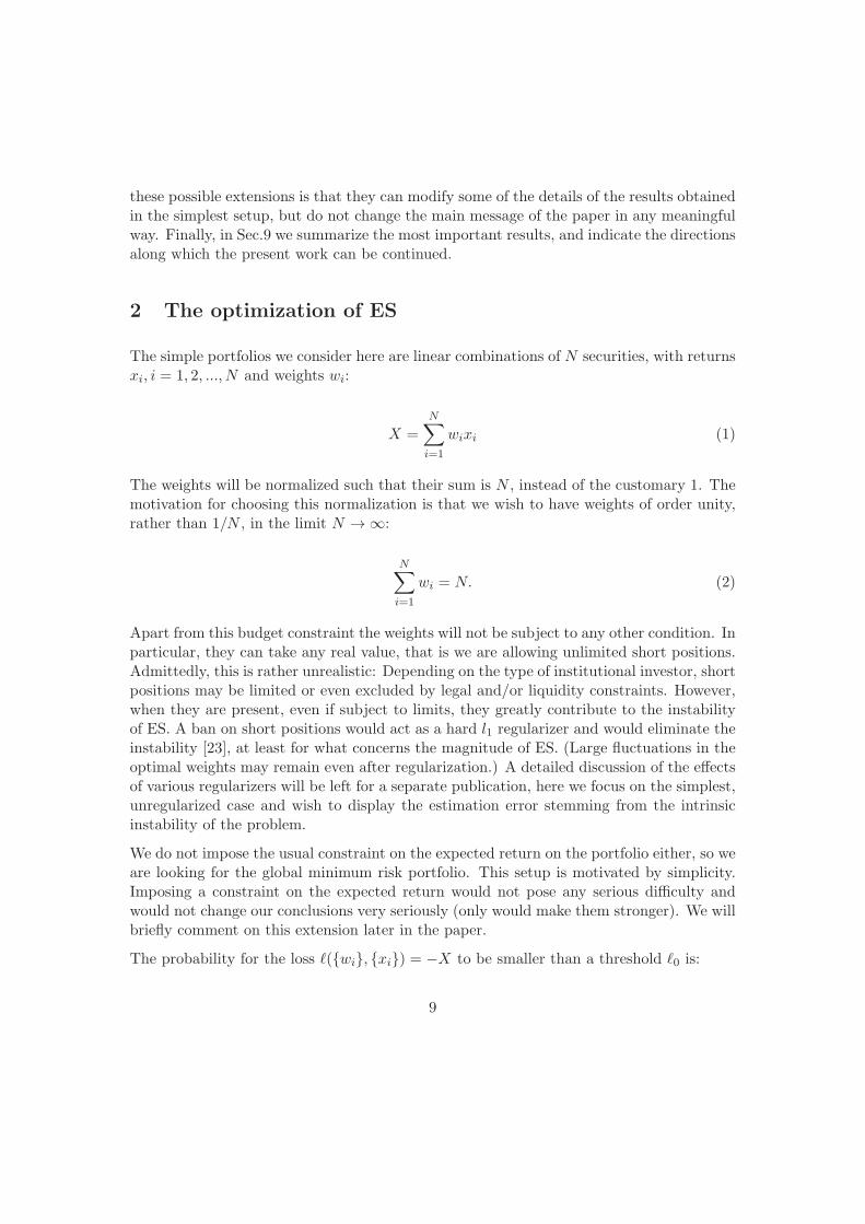
We can see from (59) that q0 diverges when r goes to rc from below: at this point theparametric estimate loses its meaning. The curve r = rc is the phase boundary for theparametric estimates for ES. It is the uppermost curve in Fig. 11 .

To obtain the contour lines we invert the formula (59) and express r as:

r =q0 − 1

q0rc(α). (62)

As can be seen, the lines belonging to a given value q0 of the estimation error are simplyscaled down from the critical line. As q0 is larger than or equal to 1 by definition, the factorin front of rc(α) varies between zero (corresponding to q0 = 1, that is to an infinitely longobservation time, N/T = 0) and one (corresponding to q0 = ∞ on the phase boundary).

5%

10%

25%

50%

100%

200%

0

0.5

1

0 0.5 1α

r

Figure 11: The contour map of the error of the parametric estimates for ES.

A few of these curves are shown in Fig. 11.

It is now easy to work out the sample size T necessary for a given relative error and a givensize N of the portfolio. Let us consider the parametric estimate of ES for e.g. a portfolioof N = 100 different securities, and stipulate a relative error of 10%, i.e. q0 = 1.1. Let usassume furthermore that the confidence level is α = 0.975 as envisaged in regulation. Thecritical value rc at this α is about 0.9, so r works out to be about 0.156. For a portfolio sizeN = 100 this means that the length of the necessary time series to ensure the 10% erroris 682 time steps (days or weeks, depending on the observation frequency of the portfoliomanager). This is a very large number, though much less than the 3500 steps needed forthe same precision in the historical estimate. Several further numerical examples are givenin Table 2.

29

estimation αerror ↓ 0.7 0.8 0.9 0.91 0.92 0.93 0.94 0.95 0.96 0.97 0.975 0.98

5% 19 16 14 14 14 14 13 13 13 13 13 13

10% 10 9 8 8 7 7 7 7 7 7 7 7

15% 7 6 5 5 5 5 5 5 5 5 5 5

20% 6 5 4 4 4 4 4 4 4 4 4 4

25% 5 4 4 4 4 4 3 3 3 3 3 3

50% 3 3 2 2 2 2 2 2 2 2 2 2

Table 2: The table shows the rounded values of T/N that are needed to have a given estimation error fordifferent values of the confidence level α used in the calculation of the parametric estimate for ExpectedShortfall.

If we are a little more demanding and prescribe an estimation error of 5%, these numberswork out to be about T = 1272, resp. 7200 for the parametric, resp. historical estimate.

Although the contour map of parametric VaR is not a subject of this paper, from [20] weknow that the difference between the ES and VaR level curves must be negligible in theregion of α’s in the vicinity of 1, thus the data requirements of parametric VaR estimationwould be as absurd as in the case of ES.

We can see that the parametric estimates are less data demanding than the historicalestimates, as expected, but they are still in a range which is totally beyond any practicallyachievable sample size.

8 Remarks on possible extensions: correlations and inho-mogeneous portfolios, fat tailed distributions, and regu-larization

We have made a number of simplifying assumptions in this study: we assumed that thefluctuations of the underlying risk factors were i.i.d. normal, disregarded all the possibleconstraints except the budget constraint, and considered the special limit N,T → ∞ withN/T finite. One may wonder how tightly these assumptions are linked to the disappointingresults for the estimation error, and whether any of them can be relaxed.

Let us first consider the question of identical distribution and independence. As shownin [20] in the case of the parametric estimates for VaR and ES, but equally true for thehistorical estimates, Gaussian fluctuations with an arbitrary (but invertible) covariancematrix can simply be accommodated in the replica formalism at the expense of some addi-tional effort and even more complicated formulae. Likewise, a constraint on the expected

30

return of the portfolio can easily be included, adding one more Lagrange multiplyer to theproblem. All these features leave the essence of our message intact, in fact, they demandeven larger samples for the same level of estimation error than in the simplified problemwe analyzed above.

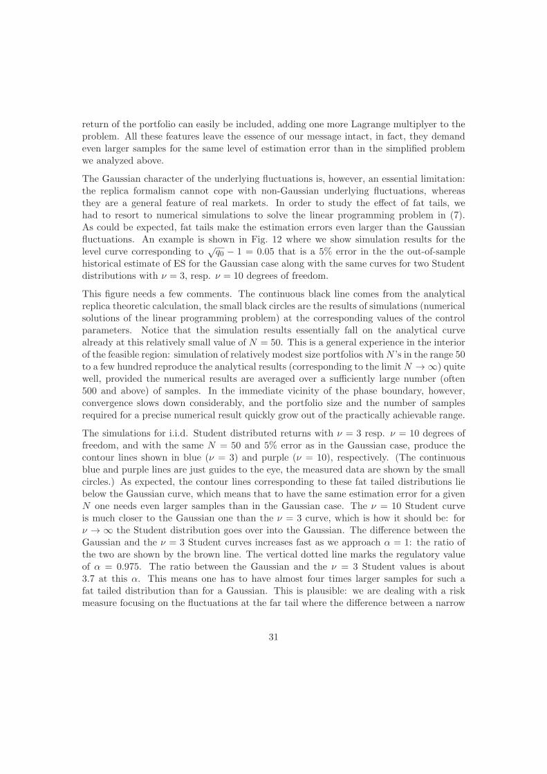
The Gaussian character of the underlying fluctuations is, however, an essential limitation:the replica formalism cannot cope with non-Gaussian underlying fluctuations, whereasthey are a general feature of real markets. In order to study the effect of fat tails, wehad to resort to numerical simulations to solve the linear programming problem in (7).As could be expected, fat tails make the estimation errors even larger than the Gaussianfluctuations. An example is shown in Fig. 12 where we show simulation results for thelevel curve corresponding to

√q0 − 1 = 0.05 that is a 5% error in the the out-of-sample

historical estimate of ES for the Gaussian case along with the same curves for two Studentdistributions with ν = 3, resp. ν = 10 degrees of freedom.

This figure needs a few comments. The continuous black line comes from the analyticalreplica theoretic calculation, the small black circles are the results of simulations (numericalsolutions of the linear programming problem) at the corresponding values of the controlparameters. Notice that the simulation results essentially fall on the analytical curvealready at this relatively small value of N = 50. This is a general experience in the interiorof the feasible region: simulation of relatively modest size portfolios withN ’s in the range 50to a few hundred reproduce the analytical results (corresponding to the limit N → ∞) quitewell, provided the numerical results are averaged over a sufficiently large number (often500 and above) of samples. In the immediate vicinity of the phase boundary, however,convergence slows down considerably, and the portfolio size and the number of samplesrequired for a precise numerical result quickly grow out of the practically achievable range.

The simulations for i.i.d. Student distributed returns with ν = 3 resp. ν = 10 degrees offreedom, and with the same N = 50 and 5% error as in the Gaussian case, produce thecontour lines shown in blue (ν = 3) and purple (ν = 10), respectively. (The continuousblue and purple lines are just guides to the eye, the measured data are shown by the smallcircles.) As expected, the contour lines corresponding to these fat tailed distributions liebelow the Gaussian curve, which means that to have the same estimation error for a givenN one needs even larger samples than in the Gaussian case. The ν = 10 Student curveis much closer to the Gaussian one than the ν = 3 curve, which is how it should be: forν → ∞ the Student distribution goes over into the Gaussian. The difference between theGaussian and the ν = 3 Student curves increases fast as we approach α = 1: the ratio ofthe two are shown by the brown line. The vertical dotted line marks the regulatory valueof α = 0.975. The ratio between the Gaussian and the ν = 3 Student values is about3.7 at this α. This means one has to have almost four times larger samples for such afat tailed distribution than for a Gaussian. This is plausible: we are dealing with a riskmeasure focusing on the fluctuations at the far tail where the difference between a narrow

31

distribution and a fat tailed one is the largest. The difference between the Gaussian and theν = 3 curves is certainly not small, but the data requirement is so unrealistic already in theGaussian case that the additional demand for fat tailed distributions is almost immaterial.

●

●

●

●

●

●●

●

●

●

●

0 0.5 1

00.

020.

04

●

●

●

●

●●

●

●

●

●

●

●

●

●

●

●

●

●

●

●

●

●

●

●

GaussStudent ν=3Student ν=10Gauss/ν=3 ratio

α

rN=50

5% error

●●

●

●

●

●

●

●

●

●

●

1

2

3

4

ratio

Figure 12: Estimation error√q0 − 1 = 0.05 contour line obtained from numerical simulations for a

portfolio size N = 50 for Gaussian (small black circles), Student ν = 3 (blue line and small blue circles) andStudent ν = 10 (purple line and purple circles) distributions. For comparison the replica theoretic result isalso presented (black line). The brown line shows the ratio of the N/T values corresponding to the same αfor the Gaussian and the Student ν = 3.

While the replica method enables us to calculate the expectation value of the relative errorof ES and the distribution of optimal portfolio weights averaged over the random Gaussiansamples, it does not provide information about how strongly these quantities fluctuatefrom sample to sample. (This is not a limitation in principle: pushing the saddle-pointcalculation in the background of the replica method one step beyond leading order, onecould derive the width of the distribution of estimation error. Such a calculation woulddemand a very serious effort and is beyond the scope of the present work.) Instead oftrying to derive the width of the distribution analytically, we have resorted to numericalsimulations again. We have found that at a safe distance from the phase boundary thedistribution of the estimated ES over the samples is becoming more and more concentrated,its width approaching zero in the N,T → ∞ limit. While the position of the peak of thedistribution stabilizes fairly fast, the convergence of the width is rather slow. An illustrationis given in Fig. 13. In the vicinity of the phase boundary, however, the average estimationerror grows beyond any bound, and there its fluctuations depend on the order of limits:if we go to the phase boundary while keeping N,T finite, the width of the distributionblows up, in the opposite limit the distribution evventually shrinks into a Dirac delta.This behaviour is in accord with what one expects to find at a phase transition.

32

05

1015

0 0.5q0 − 1

p(q 0

−1)

N=25N=50N=100N=200

N/T=0.025α=0.975

●

●

●

●

0.02

0.03

0.04

0.05

0.06

N

σq 0

25 50 100 200

Figure 13: Distribution of the estimation error over the samples from numerical simulations at N/T =0.025 for N = 25, 50, 100, 200 at the confidence level α = 97.5%. The curves were obtained by averagingover 5000, 5000, 15000, and 100 samples. The tendency of the distribution becoming sharper and sharperas N,T → ∞ is clear. Inset: the dependence of the extracted width of the estimation error distribution.The width approaches 0 in the limit N,T → ∞.

Another essential limitation of our analysis is the omission of the possible constraints on theportfolio weights. These constraints may impose limits on short selling, on different groupsof assets (corresponding to industrial sectors, geographical regions, etc.). The constraintscan (and typically do) confine the domain where the optimum is sought to a finite volume inthe space of portfolio weights. Any such constraint will act as a regularizer, and will preventthe phase transition to the infeasible region to take place. Regularizers can be built into thereplica approach, as has been demonstrated in [22,23]. However, the various possible limitsystems or regularizers introduce very different modifications to the optimization problem,and we thought their inclusion and detailed analysis would lead too far from the mainthrust of the present paper (and would at least double its length), therefore we decided toleave this important aspect of the problem to a subsequent publication.

9 Conclusions

Expanding on a short, and very preliminary, account of this work [46], in this paper weconsidered the problem of optimal portfolio selection under the risk measure ExpectedShortfall in the simplest concievable setting: we assumed that the portfolio is a linearcombination of assests with i.i.d. standard normal distributed returns and we aimed at theglobal minimum risk portfolio, omitting any constraints on the weights except the budget

33

constraint. Thus the underlying process did not have any structure at all, it was just purenoise. The basic question we asked was: for a given number N of assets in the portfolio,how large the size T of the statistical samples must be, in order for the optimization toreturn the correct optimum (with no structure and the optimal portfolio weights all equalto one another) within a prescribed estimation error. The answer we obtained in the caseof historical estimation was very discouraging: optimizing over finite samples produceda typically broad weight distribution, imaginary correlation structures and a mirage ofarbitrage. In order to obtain the correct answer within an acceptable error, we would haveneeded exceedingly large samples, far beyond any length of observation times achievablein practice. Qualitatively, this is just what one would have expected, but our results helparticulate this conclusion in a precise, quantitative manner.

Remarkably, though the results for parametric estimates turned out to be much morefavourable than those for the historical estimation, the necessary sample sizes remainedway above anything that could be regarded as realistic.

Our conclusion is thus in agreement with a number of other authors who consider the taskof optimizing large portfolios in its original (unfiltered, unregularized) form as hopeless. Toparaphrase the first sentence of the Abstract in [31]: The central message of this paper isthat nobody should be using Expected Shortfall for the purpose of portfolio optimization.One might raise the objection that ES is meant to be a diagnostic tool to measure therisk of a portfolio, not an aid to decision making concerning its optimal construction. Thismay well be the case, but the career of VaR [47] suggests that institutions will inevitablybe driven to use the new regulatory market risk measure beyond its purported scope: abinding constraint easily assumes the role of an objective function. Besides, risk is hardnot only to optimize, but as the findings of Danielsson and Zhou [11] clearly demonstrate,also to measure.

The method we applied to reach our quantitative results is, to the best of our knowledge,the only known analytical approach to the optimization of ES and led us to a closed setof equations for the relative error of the out-of sample estimate, the sensitivity to smallchanges in the returns, and for the VaR of the ES-optimized portfolio. These equationswere solved numerically; in some special cases, including that of the interesting minimaxrisk measure, by hand. The domain of applicability of our method is not limited to thetrivial case of i.i.d random variables and we plan to use it to models where the underlyingstochastic process has a structure (inhomogeneous portfolios with non-zero covariances andreturns). It will be interesting to see how large the size of samples must be in order torecover such a structure with a tolerable error.

In the present work, we deliberately left out any regularization or other dimensional re-duction method from consideration. The application of these methods is mandatory in ahigh-dimensional setting such as the present one. Their omission here is motivated partlyby trying to present, in its simplest form, a method that may be unfamiliar for most read-

34

ers, together with the nontrivial analytic results it leads to, but also by trying to keepthe length of the paper within reasonable bounds. There is a more serious consideration,however. Regularization, dimensional reduction, limits on groups of weights, or any othermethod designed to restrain the wild fluctuations of estimates, impose a certain structureon the acceptable optima thereby necessarily introducing bias. This raises the nontrivialquestion about the tradeoff between bias and fluctuation. In view of the extremely unstableestimates, a very strong regularization would be needed to stabilize them, so strong indeedas to act as a dominating Bayesian prior, basically supressing the information coming fromthe empirical samples. Faced with finite samples of real-life market data (instead of oursynthetic data), a portfolio manager may decide to entirely disregard the information com-ing from the market and go for the naive 1/N portfolio (as suggested by the result of [48]),or act on expert opinion or gut feeling, what may be happening in most cases anyhow [49].Or, worse still, she may trust a black-box optimizer package as a source of cleansed marketinformation. It is a worthy endeavour to clarify the precise quantitative conditions underwhich background knowledge can be incorporated into optimization, without bias crowdingout market information completely, and we believe the methods employed in the presentpaper in an oversimplified setting will prove to be useful in the case of more realistic marketmodels as well.

Acknowledgements

We are obliged to a number of people for useful interaction on this project, including E.Berlinger, I. Csabai, J. Danielsson, B. Domotor, F. Illes, R. Kondor, M. Marsili and S. Still.FC acknowledges support of the Economic and Social Research Council (ESRC) in fundingthe Systemic Risk Centre (ES/K002309/1). IK is grateful for the hospitality extended tohim at the Computer Science Department of the University College of London during partof the composition of this paper.

Appendix A The replica calculation

In this Appendix we show how one can deduce the cost function Eq.( 29) from the linearprogramming problem that solves the optimization of Expected Shortfall. The method istaken over from the theory of disordered systems and goes by the name of the method ofreplicas. This method was first applied in the portfolio context by Ciliberti et al. [19] andthe derivation has appeared in slightly modified forms in [21]; it is included here to makethis paper self-contained.

35

We need to find the minimum of

E[ε, {ut}] = (1− α)Tε+

T∑t=1

ut

under the constraints

ut ≥ 0, ut + ε+

N∑i=1

xi,twi ≥ 0 ∀t

andN∑i=1

wi = N.

The calculation proceeds as follows: Following the general strategy of statistical physics, wereplace the “sharp” optimization above by a “soft” one via the introduction of a fictitiousinverse temperature γ and define the canonical partition function (or generating functional)as

Zγ [{xi,t}] =∫ ∞

0

T∏i=1

dut

∫ ∞

−∞dε θ

(ut + ε+

N∑i=1

xi,twi

)e−γE[ε,{ut}], (A.1)

where θ(x) = 1 if x > 0 and zero otherwise.

The partition function is therefore an integral over all possible configurations of variablesthat are compatible with the constraints of the problem, where each configuration ε, {ut}is weighted by the Boltzmann weight e−γE[ε,{ut}]. The original optimization problem canbe retrieved in the limit γ → ∞ where only the minimal value of E[ε, {ut}] contributes.From the partition function, the minimum cost (per asset) can be computed in the limitof large N as

limN→∞

limγ→∞− logZγ [{xi,t}]

γN. (A.2)

To derive the typical properties of the ensemble we have to average over all possible real-izations of returns and compute

〈logZγ [{xi,t}]〉 =∫ ∞

−∞

N∏i=1

T∏t=1

dxi,tP [{xi,t}] logZγ [{xi,t}] , (A.3)

where P [{xi,t}] is the probability density function of returns. Averaging a logarithm isdifficult. The replica trick has been designed to circumvent this difficulty. It is based onthe use of the identity

〈logZ〉 = limn→0

∂〈Zn〉∂n

. (A.4)

36

For integer n, we can compute Zn as the partition function of a system composed of nidentical and independent replicas of the original systems. An analytical continuation toreal values of n will then allow us to perform the limit n → 0 and obtain the sought quantity〈logZγ [{xi,t}]〉. The Achilles heel of the method is the analytic continuation from integerto real n’s; the uniqueness of the analytic continuation typically cannot be easily proven.In the theory of disordered systems, the results originally obtained via the replica trickwere later verified by rigorous mathematical methods [14, 15, 42]. Such a rigorous proofhas not been constructed for the present model. However, given the convexity of our costfunction, we believe that the method is bound to lead to the correct answer. Nevertheless,with a rigorous proof lacking, we regard the replica theory as a heuristic method, so wefelt necessary to solve the linear programming problem also by direct numerical methodsto verify the results obtained via replicas.

The replicated partition function can be computed as2

Znγ =

∫ ∞

−∞

(N∏i=1

T∏t=1

dxi,t

)∫ ∞

−∞

(n∏

a=1

dεa

)∫ ∞

0

(T∏t=1

n∏a=1

duat

)∫ ∞

−∞

(N∏i=1

n∏a=1

dwai

)

×∫ i∞

−i∞

(n∏

a=1

dλa

)∫ ∞

0

(T∏t=1

n∏a=1

dμat

)∫ ∞

−∞

(T∏t=1

n∏a=1

dμat

)T∏t=1

N∏i=1

exp

{−Nx2i,t

2

}

× exp

{∑a

λa(∑i

wai −N)

}∏t

exp

{∑a

iμat

(uat + εa +

∑i

xi,twai − μa

t

)}

× exp

{−γ

∑a

(1− α)Tεa − γ∑a,t

uat

},

where we have assumed that

P [{xi,t}] =T∏t=1

N∏i=1

exp

{−Nx2i,t

2

}, (A.5)

and we have enforced the constraints through the Lagrange multipliers λa, μat and μa

t .Averaging over the quenched variables {xi,t} and introducing the overlap matrix Qa,b =1N

∑iw

ai w

bi and its conjugate Qa,b one obtains

2In the calculation we will not keep track of constant multiplicative factors that do not affect the finalresult.

37

Znγ =

∫ i∞

−i∞

(n∏

a=1

n∏b=1

dQa,bdQa,b

)∫ ∞

−∞

(n∏

a=1

dεa

)∫ ∞

0

(T∏t=1

n∏a=1

duat

)∫ ∞

−∞

(N∏i=1

n∏a=1

dwai

)

×∫ i∞

−i∞

(n∏

a=1

dλa

)∫ ∞

0

(T∏t=1

n∏a=1

dμat

)∫ ∞

−∞

(T∏t=1

n∏a=1

dμat

)exp

{∑a

λa(∑i

wai −N)

}

×∏t

exp

⎧⎨⎩−1

2

∑a,b

μatQa,bμ

bt

⎫⎬⎭ exp

⎧⎨⎩∑a,b

Qa,b

(NQa,b −

∑i

wai w

bi

)⎫⎬⎭

× exp

{−γ

∑a

(1− α)Tεa − γ∑a,t

uat

}

×∏t

exp

{i∑a

μat (u

at + εa − μa

t )

}.

We can now perform the Gaussian integral over the variables {μat }:

Znγ =

∫ i∞

−i∞

(n∏

a=1

n∏b=1

dQa,bdQa,b

)∫ ∞

−∞

(n∏

a=1

dεa

)∫ ∞

0

(T∏t=1

n∏a=1

duat

)∫ ∞

−∞

(N∏i=1

n∏a=1

dwai

)

×∫ i∞

−i∞

(n∏

a=1

dλa

)∫ ∞

0

(T∏t=1

n∏a=1

dμat

)exp

{∑a

λa(∑i

wai −N)

}

× exp

{−γ

∑a

(1− α)Tεa − γ∑a,t

uat

}exp

⎧⎨⎩∑a,b

Qa,b

(NQa,b −

∑i

wai w

bi

)⎫⎬⎭

×∏t

exp

⎧⎨⎩−1

2

∑a,b

(uat + εa − μat )Q

−1a,b

(ubt + εb − μb

t

)⎫⎬⎭ exp

{−T

2tr logQ

}.

Introducing the variables yat = μat − ubt and zat = μa

t + ubt and integrating over the {zat } weobtain

38

Znγ =

∫ i∞

−i∞

(n∏

a=1

n∏b=1

dQa,bdQa,b

)∫ ∞

−∞

(n∏

a=1

dεa

)∫ ∞

−∞

(N∏i=1

n∏a=1

dwai

)∫ i∞

−i∞

(n∏

a=1

dλa

)

× exp

{∑a

λa(∑i

wai −N)

}exp

{−γ

∑a

(1− α)Tεa − γ∑a,t

uat

}

× exp

⎧⎨⎩∑a,b

Qa,b

(NQa,b −

∑i

wai w

bi

)⎫⎬⎭

∏t

exp

⎧⎨⎩−1

2

∑a,b

(uat + εa − μat )Q

−1a,b

(ubt + εb − μb

t

)⎫⎬⎭

× exp

{−T

2tr logQ− TN log γ + T logZγ({εa, Q})

}

where

Zγ({εa, Q}) =

∫ +∞

−∞

∏a

dya exp

⎧⎨⎩−1

2

∑a,b

(ya − εa)Q−1a,b(y

b − εb)

⎫⎬⎭

× exp

{γ∑a

yaθ(−ya)

}.

In order to make further progress, let us consider the replica symmetric ansatz, in accordwith the assumption about the uniqueness of the optimum:

Qa,b =

{q1, a = bq0, a = b

(A.6)

Qa,b =

{r1, a = br0, a = b.

(A.7)

Anticipating the behaviour of the various quantities in the limit γ → ∞, we introduce thefollowing rescaling:

Δ = γ(q1 − q0), (A.8)

Δ = (r1 − r0)/γ, (A.9)

λa = λaγ, (A.10)

q0 = r0γ2. (A.11)

The �w-dependent part of the partition function is∫[Dw]e−γFw =

∫[Dw]e

∑ia λawa

i −∑

a,b Qa,b∑

i wai w

bi . (A.12)

39

Exploiting the identity log〈Xn〉 � n〈logX〉 valid for n → 0, and after some manipulations,we arrive at the following contribution to the free energy

Fw = γ⟨log

∫dw e−γ[Δw2−λw−zw

√−2q0]⟩z, (A.13)

where the notation 〈· · · 〉z means averaging over the normal variable z. After some furthermanipulations, we can write the partition function as

Znγ =

∫dλdεdq0dΔdq0dΔ e−γnNF [λ,ε,q0,Δ,q0,Δ)] (A.14)

where

F (λ, ε, q0,Δ, q0, Δ) = λ+ τ(1− α)ε−Δq0 − Δq0 (A.15)

− 1

γ

⟨log

∫ ∞

−∞dwe−γV (w,z)

⟩z+

Δ

2r√π

∫ ∞

−∞dse−s2g

(ε

Δ+ s

√2q0Δ2

),

with r = N/T ,V (w, z) = Δw2 − λw − zw

√−2q0 (A.16)

and

g(x) =

⎧⎨⎩

0, x ≥ 0x2, −1 ≤ x ≤ 0

−2x− 1, x < −1. (A.17)

The first-order conditions discussed in the main text can be obtained from the above bytaking the derivative of F with respect to its arguments (that we call the order parameters)λ, ε, q0,Δ, q0, and Δ, and setting these derivatives equal to zero.

Appendix B Solution of the first order conditions

There are some special lines on the α - r plane along which the solution of the first orderconditions simplifies significantly. Here, we study four of these lines. (The phase boundarywhere all three of the order parameters diverge was analyzed in detail in [19], so it will notbe discussed here.)

B.1 The r = 0 axis

The most obvious case is the interval 0 < α < 1 along the horizontal axis. Because r=0is here, we have full information about the underlying process, so we know that all the

40

weights are the same, wi = 1, the variance of the weights distribution is zero, hence Δ = 0and q0 = 1. This is a trivial portfolio and ε is its VaR equal to Φ−1(α). It is easy to checkthat these are the solutions of the first order conditions (51-53) indeed. Moreover, one cancalculate the first order corrections in r to them. The results are:

q0 = 1 + 2πre[Φ−1(α)]

2(1− α+

1√2π

Φ−1(α)e−12 [Φ

−1(α)]2)

, (B.1)

Δ =√2πre

12(Φ

−1(α))2

, (B.2)

ε =√q0Φ

−1(α− r

2

). (B.3)

Note that the corrections blow up at both ends of the interval, due to the divergence ofΦ−1(α) for α = 0, 1. Eq. (B.3) also requires that α > r/2.

B.2 The α = 1/2 line

Let us look for a solution such that ε = −Δ/2. Then, from the symmetries of the functionsΦ, Ψ and W , Eq. (58), we immediately see that this will happen along the vertical lineα = 0.5. The two remaining order parameters will be given by

δ ≡ Δ√q0

= 2Φ−1

(1 + r

2

),

1

q0=

δ√2πr

e−12(

δ2)

2

+δ2

4− δ2

2r. (B.4)

B.3 The ε = 0 line

If ε = 0 the first order conditions become:

r = Φ

(Δ√q0

)− 1

2, (B.5)

α =

√q0

Δ

{Ψ

(Δ√q0

)− 1√

2π

}, (B.6)

1 = Δ2

(1− 1

2r

)+

1√2π

Δ√q0

re−Δ2

2q0 . (B.7)

We can immediately see that Δ/√q0 =0 is always a solution. It corresponds to the limit r =

0 that we have already seen. The non-trivial solution exists for α > 1/2, and monotonicallyincreases with α, going to ∞ as α goes to 1. The equation of the ε = 0 line is:

α =1

2+ r +

1√2π

1

Φ−1(12 + r)

[e−

12(Φ

−1( 12+r))

2

− 1]. (B.8)

41

It is shown in Fig. 6 as the contour line with the parameter 0. It is also shown as thedotted line in the contour map of Δ, Fig. 4.

B.4 The α = 1 line

There is a further important special line where we can obtain the solution analytically.This is the vertical line at α = 1. This correponds to the minimax model also calledMaximal Loss (ML), the extremal case of ES and a risk measure in its own right [45]. Thekey point to notice is that for α = 1 the order parameter Δ diverges, but the other tworemain finite. This allows us to neglect terms that become exponentially small as Δ → ∞.Then the first of the first order conditions becomes:

r = 1− Φ

(ε√q0

)(B.9)

that immediately givesε√q0

= Φ−1(1− r) = −Φ−1(r) . (B.10)

In the following we will use the notation

ρ = −Φ−1(r) (B.11)

and

h(x) =1√2π

e−12x2

(B.12)

to simplify the formulae. The second first order condition in the same Δ → ∞ limit reads

αΔ√q0

=Δ√q0

+ ρ− ρΦ(ρ)− h(ρ) (B.13)

yieldingΔ√q0

=h(ρ)− rρ

1− α, (B.14)

while the third equation becomes

1

2Δ2=

√q0

Δ

ρ

r(1− α) +

1

2

q0Δ2

ρ

r(rρ− h(ρ)) , (B.15)

which leads to

Δ2 = r

[2√q0

Δρ(1− α) +

q0Δ2

ρ (rρ− h(ρ))

]−1

(B.16)

42

Substituting (B.15) here gives us the expression for Δ as

Δ =1

1− α

(r

ρ(h(ρ)− rρ)

) 12

. (B.17)

This shows that Δ, the sensitivity of the portfolio weights to small changes in the returns,becomes infinitely large as we approach the α = 1 limit. This limit corresponds to the bestcombination of the worst losses, so to find an infinite sensitivity to returns along this linewas to be expected.

We can now obtain the expressions for the other two order parameters:

√q0 =

(r

ρ (h(ρ)− rρ)

) 12

, (B.18)

ε =

(rρ

h(ρ)− rρ

) 12

. (B.19)

The critical behaviour of these quantitites as we approach the point r = 1/2 may be ofinterest to record:

Δ =1

2√π

1

1− α

1√12 − r

, (B.20)

√q0 ≈ 1√

2

1√12 − r

, (B.21)

ε =√π

√1

2− r . (B.22)

As we can see,√q0, the relative estimation error of ES diverges with an exponent -1/2,

while ε, the VaR of the minimax portfolio, vanishes with an exponent 1/2 in the limitr → 1/2.

Eqs. (B.17)-(B.19) in the α → 1 limit may be rewritten in the following form:

(1− α)Δ =

(r

ρ(h(ρ)− rρ)

) 12

. (B.23)

√q0 =

r

ρ

1

(1− α)Δ, (B.24)

ε = ρ√q0 , (B.25)

with ρ defined in (B.11). The behaviour of these quantities along the α = 1 line is shownin Fig. 14.

43

0.01

0.05

0.50

5.00

0 0.5

(1−

α)Δ

r0.

010.

050.

505.

000 0.5

q 0r

0 0.5

00.

5

ε

r

Figure 14: The behaviour of (1− α)Δ (left),√q0 (center) and ε (right) along the α = 1 line.

References

[1] H. Markowitz. Portfolio selection. Journal of Finance, 7:77–91, 1952.

[2] H. Markowitz. Portfolio selection: efficient diversification of investments. J. Wileyand Sons, New York, 1959.

[3] J.P. Morgan. Riskmetrics technical manual. New York: JP Morgan, 1995.

[4] Basel Committee on Banking Supervision. Overview of the amendment to the capitalaccord to incorporate market risks. Bank for International Settlements, 1996.

[5] P. Artzner, F. Delbaen, J.-M. Eber, and D. Heath. Coherent measures of risk. Math-ematical Finance, 9:203–228, 1999.

[6] G. C. Pflug. Some remarks on the value-at-risk and the conditional value-at-risk. InS. Uryasev, editor, Probabilistic constrained optimization, pages 272–281. Springer,2000.

[7] C. Acerbi and D. Tasche. Expected shortfall: a natural coherent alternative to valueat risk. Economic Notes, 31(2):379–388, 2002.

[8] C. Acerbi and D. Tasche. On the coherence of expected shortfall. Journal of Bankingand Finance, 26(7):1487–1503, 2002.

[9] Basel committee on Banking Supervision. Fundamental review of the trading book:a revised market risk framework, 2013.

[10] Basel committee on Banking Supervision. Fundamental review of the trading book:outstanding issues, 2014.

44

[11] J. Danielsson and C. Zhou. Why risk is so hard to measure. LSE Systemic Risk Centrediscussion paper No 36. Also available at http://ssrn.com/abstract=2597563, 2015.

[12] T. Hastie, R. Tibshirani, and J. Friedman. The elements of statistical learning, datamining, inference, and prediction. Second edition. Springer series in statistics Springer,Berlin, 2008.

[13] M. Mezard, G. Parisi, and M. A. Virasoro. Spin glass theory and beyond. WorldScientific Lecture Notes in Physics Vol. 9, World Scientific, Singapore, 1987.

[14] F. Guerra and F. L. Toninelli. The infinite volume limit in generalized mean fielddisordered models. Markov Proc. Rel. Fields, 9:195–207, 2003.

[15] F. Guerra and F. L. Toninelli. The thermodynamic limit in mean field spin glassmodel. Commun. Math. Phys., 230:71–79, 2002.

[16] S. Pafka and I. Kondor. Noisy covariance matrices and portfolio optimization. Eur.Phys. J., B 27:277–280, 2002.

[17] S. Pafka and I. Kondor. Noisy covariance matrices and portfolio optimization II.Physica, A 319:487–494, 2003.

[18] I. Kondor, S. Pafka, and G. Nagy. Noise sensitivity of portfolio selection under variousrisk measures. Journal of Banking and Finance, 31:1545–1573, 2007.

[19] S. Ciliberti, I. Kondor, and M. Mezard. On the feasibility of portfolio optimizationunder expected shortfall. Quantitative Finance, 7:389–396, 2007.

[20] I. Varga-Haszonits and I. Kondor. The instability of downside risk measures. J. Stat.Mech., P12007, 2008.

[21] I. Kondor and I. Varga-Haszonits. Instability of portfolio optimization under coherentrisk measures. Advances in Complex Systems, 13(03):425–437, 2010.

[22] F. Caccioli, S. Still, M. Marsili, and I. Kondor. Optimal liquidation strategies regu-larize portfolio selection. The European Journal of Finance, 19(6):554–571, 2013.

[23] F. Caccioli, I. Kondor, M. Marsili, and S. Still. Lp regularized portfolio optimization.Available at SSRN 2425326 and arXiv:1404.4040, 2014.

[24] R. T. Rockafellar and S. Uryasev. Optimization of conditional value-at-risk. Journalof Risk, 2(3):21–41, 2000.

[25] S. Ciliberti and M. Mezard. Risk minimization through portfolio replication. Eur.Phys. J., B 57:175–180, 2007.

45

[26] J.D. Jobson and B. Korkie. Improved estimation for Markowitz portfolios using James-Stein type estimators. Proceedings of the American Statistical Association (Businessand Economic Statistics), 1:279–284, 1979.

[27] P. Jorion. Bayes-Stein estimation for portfolio analysis. Journal of Financial andQuantitative Analysis, 21:279–292, 1986.

[28] P.A. Frost and J.E. Savarino. An empirical Bayes approach to efficient portfolioselection. Journal of Financial and Quantitative Analysis, 21:293–305, 1986.

[29] O. Ledoit and M. Wolf. Improved estimation of the covariance matrix of stock returnswith an application to portfolio selection. Journal of Empirical Finance, 10(5):603–621, 2003.

[30] O. Ledoit and M. Wolf. A well-conditioned estimator for large-dimensional covariancematrices. J. Multivar. Anal., 88:365–411, 2004.

[31] O. Ledoit and M. Wolf. Honey, I shrunk the sample covariance matrix. J. PortfolioManagement, 31:110, 2004.

[32] V. Golosnoy and Y. Okhrin. Multivariate shrinkage for optimal portfolio weights. TheEuropean Journal of Finance, 13:441–458, 2007.

[33] J. Brodie, I. Daubechies, C. De Mol, D. Giannone, and I. Loris. Sparse and stableMarkowitz portfolios. Proceedings of the National Academy of Science, 106(30):12267–12272, 2009.

[34] L. Laloux, P. Cizeau, J.-P. Bouchaud, and M. Potters. Noise dressing of financialcorrelation matrices. Phys. Rev. Lett., 83:1467–1470, 1999.

[35] L. Laloux, P. Cizeau, J.-P. Bouchaud, and M. Potters. Random matrix theory andfinancial correlations. International Journal of Theoretical and Applied Finance, 3:391,2000.

[36] V. Plerou, P. Gopikrishnanm, B. Rosenow, L.A.N. Amaral, and H.E. Stanley. Uni-versal and non-universal properties of cross-correlations in financial time series. Phys.Rev. Lett., 83:1471, 1999.

[37] V. Plerou, P. Gopikrishnan, B. Rosenow, L. A. N. Amaral, T. Guhr, and H. E. Stanley.A random matrix approach to cross-correlations in financial time-series. Phys. Rev.E, 65:066136, 2000.

[38] A. Kempf and C. Memmel. Estimating the global minimum variance portfolio.Schmalenbach Business Review, 58:332348, 2006.

[39] G. Frahm and C. Memmel. Dominating estimators for minimum-variance portfolios.Journal of Econometrics, 159(2):289–302, 2010.

46

[40] Y. Okhrin and W. Schmied. Distributional properties of portfolio weights. Journal ofEconometrics, 134:235–256, 2006.

[41] E. J. Elton, M. J. Gruber, S. J. Brown, and W. N. Goetzmann. Modern portfoliotheory and investment analysis. Wiley: Hoboken, NJ, 2007.

[42] M. Talagrand. Spin glasses: a challenge for mathematicians: cavity and mean fieldmodels, volume 46. Springer Science & Business Media, 2003.

[43] P. Buhlmann and S. Van De Geer. Statistics for high-dimensional data: methods,theory and applications. Springer Science & Business Media, 2011.

[44] S. Still and I. Kondor. Regularizing portfolio optimization. New Journal of Physics,12(7):075034, 2010.

[45] M. R. Young. A minimax portfolio selection rule with linear programming solution.Management science, 44(5):673–683, 1998.

[46] I. Kondor, F. Caccioli, G. Papp, and M. Marsili. Contour map of estimationerror for expected shortfall. Available at http://ssrn.com/abstract=2567876 andhttp://arxiv.org/abs/1502.0621, 2014.

[47] H. Grootveld and W. G. Hallerbach. Upgrading value-at-risk from diagnostic metricto decision variable: a wise thing to do? In G. Szego, editor, Risk measures for the21st century. John Wiley and Sons Chichester, Sussex, England, 2004.

[48] V. DeMiguel, L. Garlappi, and R. Uppal. Optimal versus naive diversification: howefficient is the 1/n portfolio strategy? Review of Financial Studies, (22):1915–1953,2009.

[49] R. O. Michaud. The Markowitz optimization enigma: is’ optimized’optimal? Finan-cial Analysts Journal, 45(1):31–42, 1989.

47