Portable X-ray Fluorescence and Nuclear Microscopy Techniques

Portable X-ray Fluorescence and Nuclear Microscopy

Techniques Applied to the Characterisation of Southern

African Rock Art Paintings

by Ruan Steyn

Thesis presented in partial fulfilment of the requirements for the degree of Master of Science in the Faculty of Science, at Stellenbosch University

April 2014

Supervisor: Prof. Paul Papka Co-supervisor: Prof. Carlos Pineda-Vargas

i

Declaration

By submitting this thesis electronically, I declare that the entirety of the work

contained therein is my own, original work, that I am the sole author thereof (save to

the extent explicitly otherwise stated), that reproduction and publication thereof by

Stellenbosch University will not infringe any third party rights and that I have not

previously in its entirety or in part submitted it for obtaining any qualification.

April 2014

Copyright © 2014 Stellenbosch University

All rights reserved

Stellenbosch University http://scholar.sun.ac.za

ii

Acknowledgement

I would like to thank a number of people for their contributions to this work. Firstly

thanks to my supervisor Prof. Paul Papka and co-supervisor Prof. Carlos Pineda-

Vargas for their support and guidance throughout the project. Dr. Leon Jacobson for

his valuable contribution as archaeology expert. Dr Brian Cross as experienced

X-ray fluorescence software analyst, for his support with the spectra analysis code.

Mr. Attie Esterhuyse, Dr. Marc Dupayrat and Dr. Mathieu Bauer from Thermo

Scientific for their assistance with the hardware and software of the Thermo

Scientific Niton spectrometer. Mr. Robert Redus from Amptek for his support on the

Amptek spectrometer. The Geology Department of the University of Stellenbosch,

specifically Ms. Cathy Clarke, and the McGregor Museum in Kimberley for making

the samples available. Dr. Cynthia Sanchez-Garrido from the Central Analytical

Facility at Stellenbosch for the standard reference materials. Prof. Shaun Wyngaardt

for his contribution. The Materials Research Department (MRD) from iThemba Labs

for the use of their facility. The National Research Foundation (NRF) for their

financial support. Lastly but definitely not the least thanks to my family and friends for

their support through this period, it is greatly appreciation.


iii

Contents

Declaration i

Acknowledgement ii

Contents iii

Abstract vii

Uittreksel ix

List of Figures xi

List of Tables xiv

List of Appendices xvi

List of abbreviations and / or acronyms xvii

CHAPTER 1 INTRODUCTION 1

1.1 INTRODUCTION 1

1.2 PROBLEM STATEMENT 2

1.3 LITERATURE REVIEW 2

1.4 RESEARCH OBJECTIVES 3

1.5 IMPORTANCE OF STUDY 3

1.6 RESEARCH METHODOLOGY 3

1.7 CHAPTER OUTLINE 4

CHAPTER 2 XRF SPECTROSCOPY AND PIXE THEORY 5

2.1 INTERACTION OF PHOTONS WITH MATTER 5

2.2 XRF PROCESS AND CHARACTERISTIC X-RAY(s) 6

2.3 LABELLING OF X-RAY TRANSITIONS 6


iv

2.4 FLUORESCENCE YIELD 8

2.5 MASS ATTENUATION COEFFICIENT 9

2.6 BREMSSTRAHLUNG 9

2.7 pXRF INTRODUCTION 11

2.8 pXRF SPECTROMETRY 12

2.8.1 X-ray Generator 13

2.8.2 Silicon Drift Detector (SDD) 14

2.8.3 Spectrometer Geometry 17

2.9 PROTON INDUCED X-RAY EMISSION (PIXE) 18

CHAPTER 3 SPECTRA EVALUATION AND CONCENTRATION EXTRACTION 20

3.1 SPECTRA SMOOTHING 22

3.2 SILICON ESCAPE PEAK 22

3.3 SUM PEAK REMOVAL 23

3.4 BACKGROUND REMOVAL 23

3.5 BLANK REMOVAL 24

3.6 INTENSITY EXTRACTION 24

3.6.1 Gaussian Peak Fitting: Linear Least Square 24

3.6.2 Gaussian Peak Fitting: Non-linear Squares 25

3.6.3 Non-Gaussian Fitting: Integrated 25

3.6.4 Non-Gaussian Fitting: Reference 25

3.7 CONCENTRATION EXTRACTION FOR PD-FP AND IOM-FP METHODS 26

3.8 LIMITATION OF THE SPECTRA EVALUATION AND CONCENTRATION

EXTRACTION 27


v

CHAPTER 4 XRF TECHNIQUE VALIDATION 28

4.1 METAL ALLOY STANDARDS 29

4.1.1 Metal rock standards results 29

4.2 COIN STANDARDS 32

4.2.1 Coin standards results 32

4.3 ROCK STANDARDS 36

4.3.1 Rock standard preparation 36

4.3.2 Rock elemental conversion to oxide 36

4.3.3 Rock standards results 37

4.4 XRF TECHNIQUE VALIDATION CONCLUSIONS 39

CHAPTER 5 EXPERIMENTAL RESULTS 40

5.1 MOUNT AYLIFF ROCK ART FRAGMENT 40

5.1.1 Compound concentrations and conclusions 42

5.1.2 Semi-quantitative comparison of the two pXRF spectrometers 48

5.2 HA KHOTSO ROCK ART FRAGMENT 49

5.2.1 Compound concentrations and conclusions 51

5.2.2 PIXE elemental distribution map 53

5.3 ROCK ART PAINT THICKNESS PROPERTIES 55

5.4 EXPERIMENTAL RESULT CONCLUSIONS 55

CHAPTER 6 CONCLUSIONS AND RECOMMENDATIONS 57

6.1 CONCLUSIONS 57

6.2 RECOMMENDATIONS 59


vi

BIBLIOGRAPHY 60

APPENDIX A: DIGITAL PULSE PROCESSOR [56] 66

APPENDIX B: PD-FP TFR INPUT FILE 68

APPENDIX C: ADMCA 75

APPENDIX D: LEVERBERG-MARQUARDT ALGORITHM 76

APPENDIX E: FP EQUATION 80

APPENDIX F: NITON XL3t AND AMPTEK SDD RESULTS FOR IRON (Fe)

ALLOY METALS 81

APPENDIX G: AMPTEK SDD AND NITON XL3t COMPOUND CONCENTRATION

RATIO VALUES FOR S, K2O, CaO AND Fe2O3 83

APPENDIX H: ELEMENTAL MAPS OF THE HA KHOTSO ROCK OBTAINED

WITH THE PIXE METHOD 85


vii

Abstract

Non-destructive portable X-ray Fluorescence (pXRF) and Particle Induced X-ray

Emission (PIXE) were used to measure the elemental concentration of rock art

fragment paintings. For pXRF the Amptek Silicon Drift Detector (SDD) and Niton

XL3t spectrometers were used to perform the measurements. These two

spectrometers use different spectrum analysis methods. The Peak Deconvolution

(PD) analysis method is used for the Amptek SDD and an Inverse Overlap Matrix

(IOM) method is used for the Niton XL3t spectrometer.

The pXRF methods were validated by using alloys, coins and rock standards. The

validation is important to establish if the pXRF technique is properly understood and

used and to advance the investigation to more complex rock art paintings, with

heterogeneous and layered properties. The elemental concentrations obtained for

the Standard Reference Materials (SRMs), which were used for the validation, were

in good agreement with that of the known concentration of the SRMs.

The two rock art fragments which were analysed from the Mount Ayliff and Ha

Khotso caves were part of larger rock art painting prior to it being naturally exfoliated

from the rock. For the Mount Ayliff rock art, seven paint points, two unpainted rock

(varnish) point adjacent to the paint and the back of the rock were analysed. The

colour of the paint ranged from black, shades of brown and shades of red. The black

paint is due to manganese or charcoal. The red colour is due to iron oxide and the

red-brown colour is due to Hematite (a type of ferrous oxide) [1]. For the Ha Khotso

fragment the paint on the front of the rock and the rock substrate (back of the rock)

were analysed.

For the Mount Ayliff rock art fragment the results for both pXRF spectrometers

indicated that the elemental concentration was uniform across the fragment. This is

due to the formation of a uniform layer of minerals such as silica and calcium

introduced by the seepage of water through the cracks of the cave. Therefore no

correlation could be established between the colour of the rock art paint and the

elements detected, as was found with the work done by Peisach, Pineda and

Jacobson [1]. For the Ha Khosto rock fragment a relation between the Ca

composition and the cream colour of the rock art paint was established. Both the

PIXE and pXRF techniques were used to identify the compound concentrations of

the Ha Khotso rock art fragment. The comparison between the two techniques

highlights the complexity of rock art paint analysis. The results from the PIXE

elemental mapping indicated the non-uniform distribution of the elements in the

analysed region.


viii

From the rock art fragment measuring the analysed points 5 times and obtaining the

same results, indicated that the particle size and inhomogeneities did not have much

effect on the compound compositions.

In order to obtain high accuracy results with pXRF, sound scientific methodology with

specific knowledge and expertise, not only about the XRF technique, but also about

the sample under investigation is required. For alloy analysis pXRF is well suited, the

analysis of geological material however more complex, since they are composed

predominately of low atomic elements e.g. silicon, aluminium, magnesium, sodium,

oxygen and carbon – all of which are excited with very low efficiencies.


ix

Uittreksel

Nie-beskadigended X-straal Fluoresensie (pXRF) en Deeltjie Geinduseerde X-straal

emmissie (PIXE) was gebruik om die elementêre konsentrasie van die rotstekeninge

in hierdie studie te bepaal. Vir die pXRF-tegniek is die “Amptek Silicon Drift Detector

(SDD)” en die “Thermo Scientific Niton XL3t” spektrometers gebruik gemaak om die

metings uit te voer. Die twee spektrometers maak gebruik van verskillende spektrum

analiseringsmetodes.Die “Peak Deconvolution (PD)” analiseringsmetode is gebruik

vir die “Amptek SDD” en die “Inverse Overlap Matrix (IOM)” analiseringsmetode is

gebruik vir die “Thermo Scientific Niton XL3t” spektrometer.

Vir die validasie van die pXRF-metode is van allooie, muntstukke en rots

standaarded gebruik gemaak. Die validasie is belangrik om vas te stel of die pXRF

tegniek behoorlik verstaan en gebruik word en om die ondersoek te bevorder na

meer komplekse rotstekeninge, met heterogene en lae eienskappe. Die element

konsentrasies wat vir die “Standard Reference Material (SRM)” wat gebruik is vir die

validasie, was in 'n goeie ooreenkoms met die van die konsentrasie van die SRM,

wat bekend is.

Die twee rotstekeninge wat ontleed is van die Mount Ayliff en Ha Khotso grotte en

was deel van 'n groter rots kuns skildery voordat hul natuurlik afgebreek het. Vir die

Mount Ayliff rotskuns, is sewe verf punte, twee ongeverfde rots (vernis) punte

aangrensend aan die verf en die agterkant van die rots ontleed. Die kleur van die

verf het gewissel van swart, skakerings van bruin en skakerings van rooi. Die swart

verf kan toegeskryf word aan mangaan of houtskool. Die rooi kleur is as gevolg van

ysteroksied en die rooi-bruin kleur is as gevolg van Hematiet ('n tipe van yster

oksied) [1]. Vir die Ha Khotso rotskuns is die verf aan die voorkant van die rots en

die rots substraat (agterkant van die rots) ontleed.

Vir die Mount Ayliff rotstekening het die resultate vir beide pXRF spektrometers

aangedui dat die elementele konsentrasie uniform oor die rotstekening is. Dit is as

gevolg van die vorming van 'n uniforme lagie van silica en kalsium, wat deur die

sypeling van water deur die krake van die grot na die oppervlak van die rotstekening

beweeg het. Daarom kon geen korrelasie tussen die kleur van die rotstekening en

die elemente wat gemeet is bepaal word nie, soos gevind deur die werk van

Peisach, Pineda en Jacobson [1]. Vir die Ha Khotso rotstekening is ‘n verband

tussen die room kleur van die rotstekening verf en Ca konsentrasie gevind. Beide die

PIXE en pXRF tegnieke is gebruik om die konsentrasies van die Ha Khotso

rotstekening te identifiseer. Die vergelyking tussen die twee tegnieke beklemtoon die

kompleksiteit van rotstekening verf analise. Die resultate van die PIXE elementele

karakterisering het aangedui die nie-eenvormige verspreiding van die elemente in

die ontlede area.


x

Deur die meting van die ontlede punte 5 keer te herhaal, en dieselfde resultate

verkry, is ‘n aanduiding dat die deeltjie grootte en inhomogeniteite nie veel invloed

op die elementele konsentrasies het nie.

Ten einde 'n hoë akkuraatheid resultate te kry met pXRF, moet goeie wetenskaplike

metode toegepas word met spesifieke kennis en kundigheid, nie net oor die XRF

tegniek, maar ook oor die rotstekening wat ondersoek word vereis. pXRF is wel

geskik vir die ontleding van allooie, die ontleding van geologiese materiaal is egter

meer kompleks, aangesien die materiaal hoofsaaklik bestaan uit lae atoomgetal

elemente bv silikon, aluminium, magnesium, natrium, suurstof en koolstof - wat almal

met lae doeltreffentheid opgewek en baie afgerem word in die materiaal.


xi

List of Figures

Figure 2.1: X-ray interaction process.

Figure 2.2: X-ray fluorescence process [13].

Figure 2.3: Transitions that give rise to the various X-ray line emissions [14].

Figure 2.4: The K and L fluorescence yield as a function of atomic number, Z [13].

Figure 2.5: Amptek SDD Compton scattering spectrum for air with a Tungsten (W)

X-ray tube.

Figure 2.6: pXRF system [13].

Figure 2.7: Transmission of X-ray from the X-ray generator [13].

Figure 2.8: Amptek SDD pXRF system setup.

Figure 2.9: Niton XL3t handheld XRF analyser [17].

Figure 2.10: Schematic cross section of a SDD with integrated FET [18].

Figure 2.11: Combination of the effect of transmission through the absorbers, such

as the Beryllium window and the dead layer of the detectors, and the

interaction in the SDD [19].

Figure 2.12: Geometry angles of a typical pXRF setup [20].

Figure 2.13: Van de Graff accelerator and NMP layout at iThemba Labs [21].

Figure 3.1: Peak Deconvolution (PD) processing steps [20].

Figure 4.1: Amptek SDD spectrometer spectrum for Brass.

Figure 4.2: Amptek SDD spectrometer spectrum for Nordic gold.

Figure 4.3: Amptek SDD spectrometer spectrum for the Krugerrand coin.

Figure 5.1: Mount Ayliff rock art fragment with the points that were characterised.

Figure 5.2: Amptek SDD spectrometer spectrum for the Mount Ayliff rock art

fragment (point 1).


xii

Figure 5.3 Elemental compositions by colour and back of the rock.

Figure 5.4: Compound and elemental concentration (wt %) per point for the

Niton XL3t spectrometer.




Amptek SDD spectrometer.



Figure 5.8: Ha Khotso rock fragment.

Figure 5.9: Amptek SDD spectrometer spectrum for the front of the Ha Khotso rock

fragment.

Figure 5.10: CaO, S, CaO and Fe2O3 concentration measurements with the Amptek

SDD and PIXE for the front and back of the Ha Khotso fragment.

Figure 5.11: K2O, TiO2, MnO and Cl concentration measurements with the Amptek


Figure 5.12: Si PIXE elemental composition map for the front of the rock.

Figure 5.13: Ca PIXE element composition map for the front of the rock.

Figure A.1: Block diagram of the Amptek SDD digital pulse processor DP5 [56].

Figure C.1: ADMCA program main display window.

Figure C.2: ADMCA window and calibrate dialog box.

Figure G.1: Amptek SDD and Niton XL3t ratio value for S at all points analysed.

Figure G.2: Amptek SDD and Niton XL3t ratio value for K2O at the analysed points.

Figure G.3: Amptek SDD and Niton XL3t ratio value for CaO at the analysed

points.

Figure G.4: Amptek SDD and Niton XL3t ratio value for Fe2O3 at the analysed

points.


xiii

Figure H.1: Mg PIXE elemental composition map for the front of the rock.

Figure H.2: S PIXE elemental composition map for the front of the rock.

Figure H.3: K PIXE elemental composition map for the front of the rock.

Figure H.4: Fe PIXE elemental composition map for the front of the rock.


xiv

List of Tables

Table 2.1: Energy level and electron configuration.

Table 2.2: PD-FP (Amptek SDD) input values.

Table 4.1: SRM categories.

Table 4.2: Niton XL3t and Amptek SDD measurements for Stainless Steel 410.

Table 4.3: Niton XL3t and Amptek SDD measurements for CDA 715 alloy.

Table 4.4: Niton XL3t and Amptek SDD measurements for Inconel-600 alloy.

Table 4.5: Niton XL3t and Amptek SDD measurements for Ti-CP (Grade 2) alloy.

Table 4.6: Brass sample concentration results.

Table 4.7: Nordic gold coin concentration results.

Table 4.8: Copper coin concentration results.

Table 4.9: XRF analysis results of the Krugerrand coin [37].

Table 4.10: Stoichiometric factors [39].

Table 4.11: SARM 48 reference material [7].


Table 5.1: Compound and element concentration of measured points 1 to 5 for

both the Niton XL3t and Amptek SDD spectrometers.

Table 5.2: Compound and element concentration of measured points 6 to 9 and

back of the rock, for both the Niton XL3t and Amptek SDD

spectrometers.

Table 5.3: Amptek SDD and Niton XL3t compound concentration ratio analysis for

K2O, CaO and Fe2O3.

Table 5.4: PIXE and Amptek SDD results for Ha Khotso rock art fragment.

Table F.1: Niton XL3t and Amptek SDD measurements for Stainless Steel 316

[57].


xv

Table F.2: Niton XL3t and Amptek SDD measurements for Al 29-4-C alloy [58].

Table F.3: Niton XL3t and Amptek SDD measurements for F-255 alloy [59].

Table F.4: Niton XL3t and Amptek SDD measurements for 20Cb3 alloy [60].


xvi

List of Appendices

APPENDIX A: DIGITAL PULSE PROCESSOR [56]

APPENDIX B: PD-FP TFR INPUT FILE

APPENDIX C: ADMCA

APPENDIX D: LEVERBERG-MARQUARDT ALGORITHM

APPENDIX E: FP EQUATION

APPENDIX F: NITON XL3t AND AMPTEK SDD FOR IRON (Fe) ALLOY

METALS

APPENDIX G: AMPTEK SDD / NITON XL3t COMPOUND CONCENTRATION

RATIO VALUES FOR K2O, CaO AND Fe2O3

APPENDIX H: ELEMENTAL MAPS OF THE HA KHOTSO ROCK OBTAINED

WITH THE PIXE METHOD


xvii

List of abbreviations and / or acronyms

CAF Central Analytical Facility

C/R Compton-to-Rayleigh ratio

FP Fundamental Parameter

FET Field-Effect Transistor

FWHM Full Width Half Maximum

IOM-FP Inverse Overlap Matrix Fundamental Parameter

JFET Junction gate Field-Effect Transistor

NMP Nuclear Microprobe

PD Peak Deconvolution

PD-FP Peak Deconvolution Fundamental Parameter

PIXE Particle Induced X-ray Emission

pXRF portable X-ray Fluorescence

ROI Region Of Interest

SDD Silicon Drift Detector

SARM South African Reference Material

SRMs Standard Reference Materials

XRF X-ray Fluorescence

Z Atomic number


1

CHAPTER 1

INTRODUCTION

1.1 INTRODUCTION

South Africa has a very rich heritage of rock art, particularly rock paintings [2] left

behind by the San hunter-gatherers, also known as Bushmen, which were the only

inhabitants of a large part of the interior of the southern Africa. These rock art

paintings can be found in caves or on rock faces, with visibility varying from very

bright to barely visible. Common themes displayed were hunting scenes, animals

and trance dance.

As the paintings are increasingly under threat of degradation, from a variety of

causes, it is vital to carry out preferably non-destructive research to determine the

elemental concentrations of rock art paint for preservation and future restoration

purposes. In addition, the elemental concentrations of rock art paint can be used to

obtain information about the raw material used during the paint preparation process,

this will however not be explored in this study.

With the successful migration of the versatile XRF analytical technique, out of the

laboratory to the field, rock art elemental concentration measurements with Portable

X-ray Fluorescence (pXRF) have become increasingly common [3]. pXRF is a

valuable technique with advantages such as, non-sample destructivity, quick

analysis, portable and easy to use in field and the laboratory, relatively user friendly

software interface and affordable equipment. Aaron N. Shugar from the Art

Conservation Department of the Buffalo State College in New York, describe this

period as an exciting time where the ongoing miniaturization of the analytical

instrumentation has advanced to a state where traditionally lab-based analysis can

now be performed in the field [4]. For pXRF the Amptek SDD and Niton XL3t

spectrometer were used with a ‘point and shoot’ methodology. Data is collected by

the spectrometer and propriety software is usually used for the determination of the

elemental concentrations. The validation of the pXRF spectrometers were done by

making use of various alloys, coins and rock reference materials.

Particle Induced X-ray Emission (PIXE) [5] which is a laboratory technique were also

used, where protons generated by an accelerator and focused onto a very small

area of the target material. PIXE is usually used to perform perform high sensitivity

elemental concentration measurements [6].

The two rock art fragments from the Mount Ayliff and Ha Khotso caves were

measured by making use of pXRF and PIXE.


2

1.2 PROBLEM STATEMENT

Since the rock art paintings degrade due to several causes such as weathering, the

need to develop preservation and restoration strategy is of vital importance. This can

be achieved by determining the elemental concentration of the rock art paint.

Additionally surface deposition information, such as composition is necessary for

patina restoration work.

The characterisation of the rock art paint can be challenging due to the fragment

size, uneven or curved surfaces and variable thickness. According to Aaron N.

Shugar, the fields of art and archaeology provide analysts with some of the most

difficult sample to characterize [4].

1.3 LITERATURE REVIEW

X-ray fluorescence has a long and diverse history as an analytical technique. The

development and miniaturization of components (detectors, X-ray tubes etc.) has

facilitated the evolution of this powerful tool into a handheld / portable device [9,10].

The range of applications includes industries such as geology, mining, environmental

and recycling. For geology pXRF is used for the characterization of rock, ores and

metals in the mining industry. In the recycling industry pXRF has established itself as

a technique of choice, due to its ability to accelerate the identification of alloys in

scrap metals. Within the archaeology field itself, there have been diverse

applications of XRF technology to analyse multiple materials. These include stones,

rock art, stone based sculpture, architectural features such as glass, corroded

metals, jewellery and museum collections. Several studies exploring the applicability

of pXRF to a variety of case studies around the world has been conducted with great

success [1,3,11,12]. These are however not the only application, many more related

studies have been performed over the last decade as the equipment has improved.

Rock art which are represented in painting, drawings and engravings are essentially

found across the world, including Africa, Australia, Southeast Asia, Europe, India,

Northern and Southern America. These rock art sites typically form a very important

part of the cultural heritage of the country and therefore the importance of developing

conservation strategies to deal with problems that threaten rock art. These threats

include water impact, salt decay, damage caused by animals and insects, soil and

vegetation cover impact, site visitors and vandalism (graffiti). As a step towards the

preservation and possible future restoration of the rock art, elemental concentration

analysis of the rock art paint is performed by using a variety of both destructive and

non-destructive techniques [1,3]. The elemental concentration of rock art paint is

usually used to obtain information about the raw material used during the paint

preparation process. Since the rock art usually consists of a large scheme of colours

ranging from black, shades of brown and shades of red, the elemental

concentrations of each individual colour is usually performed.


3

1.4 RESEARCH OBJECTIVES

This work focuses on the determination of the rock art elemental concentration of

two fragments from the Mount Ayliff and Ha Khotso caves, to investigate four

concepts:

1. Can the elements of the rock art paint be correctly identified by the two

spectrometers?

2. Are the elemental concentration results obtained from the two different pXRF

spectrometers in good agreement ?

3. Are the pXRF and PIXE results in good agreement ?

4. Is there a correlation between the colour of the rock art paint and the

elements measured ?

1.5 IMPORTANCE OF STUDY

The non-destructive elemental concentrations measurements of rock art fragments

can assist with the preservation and restoration strategies of rock art. Furthermore,

accurate elemental concentrations results are not merely achieved by trusting the

output results from the pXRF spectrometer, thorough information about the rock art

fragment investigated should be known.

1.6 RESEARCH METHODOLOGY

The validation of the analytical pXRF technique was done with homogeneous

standard reference materials (SRMs) with known composition and concentration.

The SRM included nine alloys, three coins standards and two rock standards. The

SRMs used for validation of the XRF technique where specifically selected to cover a

range of atomic numbers (13 to 82) and different combinations of atomic numbers.

The validation of the homogeneous SRMs are important, to advance the

investigation to unknown heterogeneous layered samples, such as the rock art

paintings from the Mount Ayliff and Ha Khotso caves.


4

1.7 CHAPTER OUTLINE

Chapter one provided an overview of the importance, objectives and research

methodology followed for this study. A literature review of relevant previous studies

conducted to determine elemental concentration of rock art paint, with similar

techniques is also included.

Chapter two cover the pXRF and PIXE theory which include concepts such as

interaction of photons with matter, characteristic X-ray(s), labelling of the X-ray

transitions, fluorescence yield, mass attenuation coefficients and bremsstrahlung.

These concepts are fundamental to the understanding of the techniques. The

experimental setup and components of each technique is also discussed.

Chapter three discusses the spectra evaluation and concentration extraction

methodology followed.

Chapter four will provide the results of the pXRF technique validation. This is

important to establish if the pXRF technique is properly understood and used.

Chapter five will provide the results of the measurements done on the rock art

fragments. This chapter will also indicate if the elements are correctly identified and if

there is a significant difference between the results for the different techniques.

Finally, chapter six will conclude the study and offer recommendations.


5

CHAPTER 2

XRF SPECTROSCOPY AND PIXE THEORY

2.1 INTERACTION OF PHOTONS WITH MATTER

The interaction of the X-ray(s) with matter can either be by absorption or scattering

process. In materials with finite thickness some of the X-ray(s) can also be

transmitted, as illustrated in Figure 2.1. The favoured process depends on the

sample thickness, density, composition and the incident X-ray energy.

The absorption process occur when the X-ray interact with the absorbing material at

atomic level to transfer its entire energy and causes XRF, which form the basis of

XRF spectroscopy. Scattering involve the deflection of the incident photon with the

scattered material, this can occur both with energy loss (Compton scattering) or

without energy loss (Rayleigh scattering). Compton Scattering is the interaction

between the incoming photon with the atoms of the target material which causes the

photon to change direction.

Rayleigh Scatter Incident X-ray Fluorescence

Compton Scatter

Transmitted X-ray(s)

Figure 2.1: X-ray interaction process.


6

2.2 XRF PROCESS AND CHARACTERISTIC X-RAY(S)

For the Photoelectric absorption process to occur the energy of the photon needs to

be equal or higher than the binding energy of the electron. An inner shell electron

which is ejected after the incoming photon is completely absorbed leaves the atom in

a highly excited state, since a vacancy has been created in one of the inner shells.

The atom will return to its neutral state with the emission of a characteristic X-ray

photon specific to the atom, also known as XRF and demonstrated in Figure 2.2. The

energy difference between the ejected and replaced electron is characteristic of the

element atom in which the fluorescent process occur. This is the key feature of XRF

for elemental identification purposes.

Figure 2.2: X-ray fluorescence process [13].

2.3 LABELLING OF X-RAY TRANSITIONS

With each unique atom having a number of available electrons and with all having

different possible de-excitation routes, a set of selection rules have been defined to

account therefore. Each electron in an atom can be defined by a set of four unique

quantum numbers: n, l, m and s. The principal quantum number n take all integral

values, with n = 1 being the K level and n = 2 the L level, the angular quantum

number l taking all the values from n - 1 to zero, the magnetic quantum number m

taking value from + l to – l and the spin quantum number s with a value of ± 1/2.

The total momentum J of an electron is given by the vector sum of l + s.


7

The production of diagram lines requires that the principal number change by at least

one (∆ n >= 1), the angular quantum number must change by at least one (∆ l = ± 1),

and the J quantum number must change by zero or one (∆J = 0, ±1). Hence not all

transitions from the outer shells or subshells are allowed, only those obeying the

selection rules for electric dipole radiation. The transition that is not allowed is called

forbidden lines, which arise from outer orbital levels where there is no sharp energy

distinction between the orbitals.

The theory of X-ray spectra shows the existence of a limited number of allowed

transitions, the rest is “forbidden”. The X-ray lines and energy levels are shown in

the Figure 2.3 and Table 2.1:

Figure 2.3: Transitions that give rise to the various X-ray line emissions [14].

Table 2.1: Energy level and electron configuration.

Energy level Principle number n

Angular number l

Total momentum j

Electron configuration

N7 4 3 7/2 4f7/2

N5 4 2 5/2 4d 5/2

N3 4 1 3/2 4p 3/2

N1 4 0 1/2 4s

M5 3 2 5/2 3d5/2

M3 3 1 3/2 3p3/2

M1 3 0 1/2 3s

L3 2 1 3/2 2p3/2

L2 2 1 1/2 2p½

L1 2 0 1/2 2s

K1 1 0 1/2 1s


8

For example when an electron ejected from a K shell, the electron vacancy will be

filled by an electron coming from the L shell. The transition is accompanied by the

emission of an X-ray line known as the K�line and leaves a vacancy in the L shell. If

the atom already has sufficient electrons, the K shell vacancy might be filled by an

electron coming from an M level that is accompanied by the emission of the �� line.

All the energies of the principal X-ray emission lines for the K and L shell can be

found in Appendix II, Table 4 of Reference [15].

2.4 FLUORESCENCE YIELD

For an electron to be expelled from one of the orbitals, the X-ray energy must

exceed to binding energy of the electron. Below the binding energy a drop in

absorption is observed since the energy is not sufficient to emit electrons from that

shell and too high in energy to emit electrons form the lower energy shells. If the

energy is too high only a few electrons will be knocked out. As X-ray energy reduces

and approaches the electron binding energy, the yield of the expelled electrons

increases.

Since not all incident X-ray(s) result in the emission of characteristic X-ray(s)

fluorescence, fluorescence yield is the ratio of fluorescence X-ray(s) to incident X-

ray(s), as illustrated in Figure 2.4.

Figure 2.4: The K and L fluorescence yield as a function of atomic number, Z [13].

From Figure 2.4 it can be seen that the yield is low for light elements and high for

heavy elements, this is mainly due to the Auger effect. This is a phenomenon were

the filling of an inner shell vacancy of an atom is accompanied by the emission of an

electron from the same atom i.e. instead of X-ray fluorescence, emission energy can

be transferred to another electron, which is ejected from the atom. A consequence of

the Auger effect is that the actual number of X-ray photons produced from an atom is


9

less than expected, since the vacancy in a given shell might be filled through non-

radiative transition. Auger electrons are predominately produced during relaxation of

K-shell ionisation of light elements (Z < 20) [15].

2.5 MASS ATTENUATION COEFFICIENT

The attenuation coefficient is the quantity that characterise how easily the material

can be penetrated by an X-ray. A large attenuation coefficient is an indication that

the X-ray is quickly attenuated (weakened) as it passes through the medium and a

small attenuation coefficient means that the X-ray goes through the material quite

easily.

The mass attenuation coefficient �(�� ) is defined as the ratio of linear attenuation

coefficient and the density of the material. The equation for the linear attenuation

coefficient µ* per centimetre of travel in the absorber is:

�∗ � �� = ��

��

� �

where� is the density of the medium and �� is Avogadro’s number.

Where �� is the sum of the probability for each of the competing interaction

processes. The sum of these cross sections is normalized to a per atom basis

�� = � +� +⋯

where � is the total Photoelectric absorption cross section per atom and � the

Compton collision cross section.

2.6 BREMSSTRAHLUNG

Bremsstrahlung occurs following the deceleration (loss of energy) of the electrons

within the material, due to the interaction of the impinging electrons with the target

elements. Hence at each collision as the electrons are decelerated part of the kinetic

energy is lost and emitted as X-ray photons.

During a collision with material an electron can lose any amount of energy between

zero and Emax which results in a bremsstrahlung continuum with energies in that

range, as presented in Figure 2.5. The characteristic lines of Tungsten (W) and

Argon (Ar) are superimposed on the bremsstrahlung continuum. The W is introduced

from the anode material and the Ar from the air space between the sample and

detector.


10

Figure 2.5: Amptek SDD Compton scattering spectrum for air with a Tungsten (W) X-ray tube.


11

2.7 pXRF INTRODUCTION

XRF spectroscopy is the technique used to analyse fluorescent X-ray(s), in order to

determine the elemental composition of a particular material. The components of the

pXRF device are a source of X-ray(s), a sample, detector, spectrometer and

processor (computer), as illustrated in Figure 2.6.

Figure 2.6: pXRF system [13].

The operating principle of an X-ray generator is to pass an electric current through a

filament which causes electrons to be emitted. These electrons are then accelerated

by high voltage (typically 25 – 50 kV) towards an anode (which is typically made of

Ag or W material). The deceleration of the electrons (when they hit the anode

material) causes an X-ray continuum to be emitted, known as Bremsstrahlung.

Additionally a fraction of the electrons will cause characteristic X-ray fluorescence

from the anode material. Hence the energy spectra from the X-ray generator will be

the characteristic fluorescence lines from the target material superimposed on the

broad bremsstrahlung continuum. This energy spectrum is then directed to the

sample through the Beryllium (Be) window, as illustrated in Figure 2.7.

Figure 2.7: Transmission of X-ray from the X-ray generator [13].

X-Ray(s)

Electrons


12

The X-ray detector converts X-ray photon energies into measureable and countable

voltage pulses. This is done by photoionization, where the interaction between the

incoming X-ray photon and the active detector material produces an energetic

electron which in turn produces many more. The incident X-ray is therefore

essentially absorbed by the detector material, and causing one or more electron-hole

pairs to form. The energy to do this is fixed for that particular material and therefore

the X-ray will form as many electron-hole pairs as its energy will allow. These

electrons are pulled of the detector to produce a current (which is proportional to the

number of electron-hole pairs and directly related to X-ray energy) and converted

into a voltage with amplitude proportional to the incident energy, by using a capacitor

and resistor i.e. a voltage is thus generated for every X-ray photon that enters the

detector.

The pre-amplification and processing electronics are then employed to maintain the

linearity of the voltage signal with respect to the original charge pulse. In other words

the rate at which the voltage signal is recorded is the same as the rate at which the

X-ray photons enter the detector.

Therefrom, the multichannel analyser accumulates an energy spectrum of the

sequential events in a histogram memory. The counts associated with a photon of a

specific energy should hypothetically end up in a signal channel, but are distributed

in a Gaussian fashion over several adjacent channels in the spectrum due to the

statistical fluctuations in the number of electron-hole pairs created when an X-ray of

a given energy enters the detector.

2.8 pXRF SPECTROMETERS

The two pXRF spectrometers used are the Amptek Silicon Drift Detector (SDD) and

the Niton XL3t, with a Tungsten (W) and Silver (Ag) X-ray anode tube respectively,

as demonstrated in Figure 2.8 and Figure 2.9. Both the spectrometers are capable of

40 kV excitation energy and uses SDD for detection. The spectrometers were placed

as close as possible to the sample to minimize the X-ray attenuation by air,

especially for the low energy X-ray(s) [16].

Figure 2.8: Amptek SDD pXRF system setup.

Tungsten (W) X-ray tube

Silicon Drift Detector and

multichannel pulse-height

analyser (MCA)

Sample


13

Figure 2.9: Niton XL3t handheld XRF analyser [17].

2.8.1 X-ray Generator

For the Tungsten (W) anode material, the L line is most effectively used for the

exciting of light elements in the range of 1 - 10 keV, since the Lβ line and Lα line for

W is at 9.81 keV and 8.36 keV respectively. For higher energy lines for example

Zirconium Zr Kα at 15.78 keV the L lines of W provide no excitation as they are lower

in energy than the absorption edge of the Zr K line at 17.99 keV. Hence the

bremsstrahlung hump provides the excitation. For Ag as anode material the Kβ, Kα,

Lβ and Lα line energies are at 25.20 keV, 22.08 keV, 3.25 keV and 2.99 keV,

respectively.

The energy distribution directed towards the target governs the effectiveness of

excitation and hence the importance of selecting the most optimal

excitation energy (eV) and accelerating voltage (kV). The limited counting capacity of

the detector and the multi-elemental samples are adding complications to the

derivation of the optimum excitation conditions. For X-ray fluorescence to be

generated it is necessary to have incident X-ray energies above the absorption edge

of the elemental line series that needs to be excited. A general rule of thumb is to

use an X-ray tube voltage of about 1.5 to 2 times higher than the absorption edge of

interest.


14

2.8.2 Silicon Drift Detector (SDD)

The SDD consists of a volume of n-type silicon bulk depleted from both sides: a

homogeneous, shallow p+-n junction on the side where the incoming radiation enters

the detector and a structure of circular p+ drift rings on the opposite side as shown in

Figure 2.10.

Figure 2.10: Schematic cross section of a SDD with integrated FET [18].

By applying a negative voltage on the homogeneous back side (radiation entrance

window) and an increasingly negative voltage on the drift rings, a potential field

distribution is created inside the detector such that the electrons generated by the

absorption of ionizing radiation drift towards a small sized collecting anode situated

in the centre of the device. The detector spectroscopic performance is improved by

integrating the first amplification stage (a JFET transistor as shown in Figure 2.10)

directly into the sensor. The connection of the anode to the transistor gate is reduced

to a small metal strip of a few microns length, which suppress some electronic noise.

In order to minimize the noise from these thermally generated charges, the detector

crystal (active part of the detector) must be kept cold throughout the time the bias is

applied. This is produced by thermoelectric, Peltier cooling. If cooling is lost or

degrades over time the automatic bias shutoff system (temperature sensor) will be

activated, which will switch the detector off. Cooling is further essential to minimise

the detector leakage current, the main source of noise in a detector, which is derived

from the generation of charge carriers in the absence of X-ray(s) through the thermal

vibration of the detector crystal lattice. Additionally the detector head (crystal and

FET) is enclosed within vacuum, which is retained by a thin (typically 5-50 µm)

beryllium entrance window. Any H2 escaping through the window degrades the high

vacuum and leads to increased temperature, leakage current and deteriorating

performance.


15

Important feature of a detector is the energy resolution. This the precision with which

the energy of specific X-ray(s) photons can be determined. Energy resolution is

usually expressed as Full Width Half Maximum (FWHM) of the pulse-height

distribution measured at a specific energy. With the 7 mm2 Amptek SDD detectors a

FWHM of approximately 140 eV at 5.9 keV for a shaping time (the time constant of

the detector) of 9.6 µs is achievable. The resolution of the Niton XL3t varies between

145 to 165 eV for a shaping time of 4 µs or between 155 to 175 eV for 1 µs shaping

time.

The FWHM might give a good indication of the quality of the detection system, but

other factors such as the maximum count rate, the presence of background and

artifacts is of similar importance.

The measured FWHM of the X-ray line (∆ETotal) is the quadratic sum of the

contribution due to the detector intrinsic resolution processes (∆EDet) and that

associated with the electronic pulse processing system (∆EElec) [15]:

"#$��% =&"#'(�) + "#*%(�) . (3.1)

The contribution to resolution associated with electronic noise (∆EElec) is due to

random fluctuations in thermally generated leakage currents within the detector and

in the early stages of the amplifier components, which are intrinsic processes to the

overall measurement process. ∆EDet is a result of the statistics of the free-charge

production process occurring in the depleted volume of the SDD.

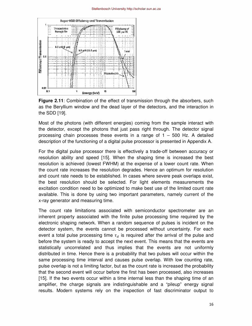
The intrinsic full energy efficiency of a detector corresponds to the probability that an

X-ray will enter the front of the detector and deposit all its energy inside the detector

via the photoelectric effect. Near-unity intrinsic efficiencies for the detector over a

wide range of X-ray energies (2 keV to 15 keV) are can be seen in Figure 2.11 for

the Amptek SDD. The high-energy limits are established by the photoelectric cross

section of the detector material (silicon) and the thickness of the active depth of the

SDD (500µm). The low-energy cutoff is determined by the thickness of the Beryllium

window either 0.3 mil (8 µm), 0.5 mil (12.5 µm) and 1 mil (25 µm) as well as the

presence of a thin absorbing layer and dead layer on the surface of the detector. The

thin absorbing layer is for protection purposes and the dead layer, which is

effectively inactive and no charge can be collected.


16

Figure 2.11: Combination of the effect of transmission through the absorbers, such

as the Beryllium window and the dead layer of the detectors, and the interaction in

the SDD [19].

Most of the photons (with different energies) coming from the sample interact with

the detector, except the photons that just pass right through. The detector signal

processing chain processes these events in a range of 1 – 500 Hz. A detailed

description of the functioning of a digital pulse processor is presented in Appendix A.

For the digital pulse processor there is effectively a trade-off between accuracy or

resolution ability and speed [15]. When the shaping time is increased the best

resolution is achieved (lowest FWHM) at the expense of a lower count rate. When

the count rate increases the resolution degrades. Hence an optimum for resolution

and count rate needs to be established. In cases where severe peak overlaps exist,

the best resolution should be selected. For light elements measurements the

excitation condition need to be optimized to make best use of the limited count rate

available. This is done by using two important parameters, namely current of the

x-ray generator and measuring time.

The count rate limitations associated with semiconductor spectrometer are an

inherent property associated with the finite pulse processing time required by the

electronic shaping network. When a random sequence of pulses is incident on the

detector system, the events cannot be processed without uncertainty. For each

event a total pulse processing time �+ is required after the arrival of the pulse and

before the system is ready to accept the next event. This means that the events are

statistically uncorrelated and thus implies that the events are not uniformly

distributed in time. Hence there is a probability that two pulses will occur within the

same processing time interval and causes pulse overlap. With low counting rate,

pulse overlap is not a limiting factor, but as the count rate is increased the probability

that the second event will occur before the first has been processed, also increases

[15]. If the two events occur within a time internal less than the shaping time of an

amplifier, the charge signals are indistinguishable and a “pileup” energy signal

results. Modern systems rely on the inspection of fast discriminator output to


17

determine if two pulses have occurred in rapid succession. Logic is used to gate the

output of the processor to eliminate the resultant uncertain energy signal and

produces an uncertain pileup energy output [15].

2.8.3 Spectrometer Geometry

The geometric angle values for the Amptek SDD which form part of the input values

for the Peak Deconvolution Fundamental Parameter (PD-FP) method are shown in

Table 2.2 and schematically illustrated in Figure 2.12. These angle input values

together with information about the equipment properties from part of the PD-FP

TRF input file, as presented in Appendix B.

Table 2.2: PD-FP (Amptek SDD) input values.

Figure 2.12: Geometry angles of a typical pXRF setup [20].

For the Niton XL3t spectrometer there is no need to provide the analysis software

with the geometry, since the experimental angle values are fixed and encoded in the

software. From the Niton XL3t product specification the values of the θtube-and-surface

and θdetector-and-surface is given as 71⁰ and 61⁰ respectively.

Input parameters Value

Distance between tube-sample (mm):

15

Distance between sample-detector (mm) :

15

Incident angle (⁰) 45

Take-off angle (⁰) 45

Scatter angle (⁰) 90

Alpha angle (⁰) 0


18

2.9 PROTON INDUCED X-RAY EMISSION (PIXE)

The nuclear microprobe is used for quantitative nondestructive microanalysis for

various fields including, material science, geology and biomedicine. This is due to

the significant progress that has been made with the instrumentation hardware, such

as lenses, collimator slits, data acquisition systems and target chambers. The

nuclear microprobe combined with PIXE, can detect trace elements to the

sensitivities of a few ppm (or even sub ppm) concentrations.

A schematic of the 6 MV Van de Graaff Accelerator equipped with a Nuclear

Microprobe (NMP) at iThemba Labs, is shown in Figure 2.13.

Figure 2.13: Van de Graff accelerator and NMP layout at iThemba Labs [21] (with

the most important features shown, which distances in-between shown in mm).

The Van de Graaff accelerator accelerates ions vertically downwards, with energy

stabilisation and beam selection made by a 90⁰ analysing magnet. The ions then

travel through a horizontal flight path to the target. After the analysing magnet, the

ions travel through the energy stabilisation slits situated in front of the main

beamstop. Ions then pass through a quadrupole duplet for focusing of the beam at

the object slits. Before the object slits, the beam passes through a switching magnet

with a narrow entrance port in the Y direction (1.2 mm), which is used for the beam

lines at an angle to the NMP line. The primary beam is then allowed to pass through

the object slits with a diameter of 1 mm [21].

A beam current of between 50–100 pA is transmitted through the collimator with the

use of a variable slit. This allows the use of intense beams, for achieving the

smallest beam spot size possible.


19

The target chamber is pumped down with a diffusion pump backed by a roughing

pump; this allows for quick sample changing and higher throughput. The target

chamber is the standard Oxford NMP chamber. The features include an X-ray

detector situated 35 mm away from the target at 135º to the incoming ion direction,

an annular Si surface barrier (SSB) detector situated close to 180º, channeltron

electron detector for secondary electron imaging, electron suppression ring in front

and behind the target and the optical microscope at 45º with respect to the normal to

the sample surface. The target chamber allows for the stepper motor control of the

samples for X, Y and Z axes. Signals from the detectors are fed to the normal

electronic units for amplification and digitisation [21].

The data is collected by using the XSYS [22] acquisition system, with event-by-event

storing capability, and the GeoPIXEII software package [23] is used for the extraction

of the elemental concentrations, from the raw spectra.

For PIXE analysis the target material is bombarded with ions of sufficient energy

(usually protons with energy in megaelectron volt (MeV) range) generated by an

accelerator, instead of X-ray(s) as in the case of XRF.

The Ha Khotso rock art surface was scanned using a proton probe (microprobe),

with energy of 3.0 MeV over an area of approximately 0.8 mm2. The beam was

focused to a minimum spot size of 3 µm2 with a current of 100 pA. The scanned area

were analysed in a rectangular pattern divided in a map size of 128 x 128 pixels, with

a dwell time of ~10 ms/pixel. For the elemental mapping, PIXE and proton

backscattering spectra were acquired simultaneously in event-by-event mode, using

a Si (Li) PGT Pentafet X-ray detector with a 3.0 mm thick Si crystal. The detector

diameter, surface area and resolution (FWHM) is 6.18 mm, 29.99 mm2 and 160 eV at

5.898 keV for Mn, respectively. The count rate was kept below 1000 counts/second

to avoid pulse pile-up and to achieve acceptable counting statistics. For the analysis

of light elements such as Na and Mg, a proton probe with energy of 1.5 MeV and

lateral resolution of approximately 2.5 µm2 were used. Additionally a 25 µm Be

absorber was used to stop the scattered ions reaching the detector.


20

CHAPTER 3

SPECTRA EVALUATION AND CONCENTRATION EXTRACTION

Spectrum evaluation uses mathematical techniques to extract peak intensities from

the spectrum, which can be used to determine the elements and their concentration.

This is done by using Peak Deconvolution Fundamental Parameter (PD-FP) or

Inverse Overlap Matrix Fundamental Parameter (IOM-FP).

The PD-FP process is a series of steps used to remove the undesirable occurrences

which contribute to the spectra. These steps are illustrated in Figure 3.1. The PD

process relies heavily on mathematical techniques to extract useful information;

therefore it is important to employ optimal experimental conditions to obtain the

spectra, since this will determine the effectiveness of the PD process. Optimal

conditions can be achieved in a number of ways either by increasing the counting

statistics or by keeping the dead time low. Additionally control over the distance from

the sample to the detector is essential to obtain enough statistics for the lower

energy lines of the low atomic number elements. Factors internally performed by the

electronics of the system such as keeping the detector cold and maintaining the

stability of the high voltage power supply are of similar importance.

The IOM-FP process is an accelerated spectrum processing method which is much

faster than the PD-FP spectra process. The IOM-FP process is usually required for

certain applications where results are needed within a few seconds. This is done by

using calibration standards with known Compton-to-Rayleigh (C/R) peak intensity

ratios to generate calibration curves (XRF C/R peak intensity ratio versus atomic

number). These curves are then use to determine the elements from the spectra.

Since the elemental and corresponding peak intensity is known, the elemental

concentration can be determined with the FP equations. Full detail of the IOM-FP

spectra process is however not known, since it is propriety company information.

Prior to sample measurement an energy calibration needs to be performed. This is

done by taking measurements of calibration standards with known elemental

composition; since the exact energy of these elements are known [15]. The ADMCA

display window for the calibration is presented in Appendix C.

The goal of quantitative XRF is to determine the concentration of the elements

present in the sample; this is done by using the FP equations. A first estimate of the

concentration is evaluated, from the measured intensities with the FP method,

proposed by Criss and Birks [25]. This estimate is then used to calculate a new set

of intensities from which a new revised estimate of composition is calculated. This

process is iterated until the difference between two consecutive iterations becomes


21

insignificant. The main advantage of the FP equation is its theoretical exactness and

the ability to correct for matrix effects. However a first estimate is necessary for this

method to function properly. Frequently a poor first approximation is generated from

measured intensities, because such intensities have been strongly modified by

matrix effects. Matrix effects are the result of variations in the physical character of

the sample and include parameters such as particle size, uniformity, homogeneity

and surface condition [26].

The FP equations are calculated each iteration, which can cause the analysis

process to be lengthy and slow. This is due to a large number of iterations which is

sometimes required, since the first approximation of the composition is often very far

from the final composition [27].

Figure 3.1: Peak Deconvolution (PD) processing steps [20].

Spectra smoothing

Si escape peak removal

Sum peak removal

Background removal

Blank removal

Intensity extraction


22

3.1 SPECTRA SMOOTHING

The smoothing technique is ideal to remove or suppress statistical fluctuations, such

as fictitious maxima which occur on both the continuum and on the slope of the

characteristic peaks. Statistical fluctuations occur due to the uncertainty on each

channel content yi. The technique reduces the uncertainty in the data locally and

redistributes the original channel content over the adjacent channels.

To smooth the fluctuating signals the moving average technique can be employed.

For a measured spectrum y, a smoothed spectrum y* is obtained, by calculating the

mean channel content around each channel i [15]:

,∗- = ,.- = �)/� ∑ ,-/1/123 . (3.1)

The smoothing effect depends on the width of the filter, 2m+1. The filter can however

introduce peak distortions, which depends on the filter-width-to-peak-width ratio. The

peak distortion is caused by the fact that for the calculation of ,∗- , the content of all

adjacent channels is used with equal weight. These peak distortions and broadening

can be minimized by using a non-uniform filter with some weighing function that

place more weight on the central channels and less on the edge of the filter [15]:

,∗- = �� ∑ ℎ1,-/112123 (3.2)

where hj are the convolution integers and N is a suitable normalization factor.

3.2 SILICON ESCAPE PEAK

If the energy of the incoming X-ray(s) is higher than the Si K absorption edge at

1.832 keV, it can produce characteristic Si Kα X-ray(s) (E = 1.739 keV) from the XRF

detector material, called escape peaks. Most of the Si K X-ray(s) will immediately be

absorbed within the detector volume, because of their low energy and short range in

materials. There is however a non-zero probability that the Si Kα X-ray(s) produced

will escape from the detector volume and not contribute to the charge collected from

the primary photon that was detected. The resulting lower energy peak is called Si

escape peak. This usually occurs after photoelectric absorption of the impinging

X-ray photon near the edge regions or the front of the detector crystal. The energy

deposited in the detector by the incoming X-ray is therefore reduced by the escaping

SiK photon energy (the escape peaks are at expected 1.739 keV (Si Kα) below the

parent peak). At energies of above 10 keV the Si escape peak effect can effectively

be negligible [15], since the X-ray(s) are more penetrating and hence interact deeper

in the material before they undergo photoelectric absorption, hence the SiK X-ray(s)

do not come out. For energies below 10 keV, the Si escape peak is removed by the

PD-FP method and added back to their parent peak.


23

3.3 SUM PEAK REMOVAL

Sum peaks arise from a specific form of peak (pulse) pileup, where two events from

high-intensity peaks occur in the pulse processing electronics shortly one after the

other, without the pileup inspector recognizing them as two separate events. The

signal is thus seen as one and the energy is registered as the sum of the two.

Therefore it needs to be removed from the spectra by the PD-FP method.

This can either be for two elements from the same sample or the same elemental

peak e.g. Si (Kα of 1.74 KeV) and Al (Kα of 1.487KeV) and hence a peak at 3.23 KeV

is detected or the sum of two Si Kα events at (3.48 keV). The sum peaks are unlikely

to be identified as a different element, but they may interfere with important lines in

the analysis.

The intensity of the sum peak is count rate dependant and an effective way to

reduce the effect of the sum peak is to reduce the count rate [15]. Furthermore a

short pulse shaping time is important, to optimize the detection pulses which are

closely spaced in time.

3.4 BACKGROUND REMOVAL

The detector background is mainly the result of fundamental X-ray and electron-

energy loss processes i.e. the coherent and incoherent scattering of the excitation

X-ray(s). Other effects contributing to the background are the effects associated with

the partial collection or incomplete charge collection, usually producing tailings,

which are higher than the expected continuum.

The background removal is done by the peak stripping method, which is based on

the removal of rapidly varying structures in a spectrum by comparing the channel

content yi with the channel content of its neighbours [15]:

5- = 67/6789) . (3.3)

If yi is smaller than mi , the content of channel i is replaced by the mean mi .By

repeating this procedure, the peaks are gradually “stripped” from the spectrum.

The method does however pick up local fluctuations in the continuum, which is

caused by the Be window. The Si internal fluorescence peak and absorption edge

caused by the dead layer effects can further cause fluctuations in the continuum.


24

3.5 BLANK REMOVAL

This method is mainly used for the removal of the Argon (which fluorescence in air)

and X-ray tube scattering peaks. This method uses a channel-by-channel subtraction

of the blank counts from the corresponding counts in the spectrum. For this method it

is assumed that a blank sample is acquired under the same conditions as the normal

spectra e.g. live-time, X-ray beam parameters and the spectra is evaluated via all the

prior mentioned methods i.e. smoothing, escape peak removal, background removal.

3.6 INTENSITY EXTRACTION

After the spectra processing steps have been carried out, the final step is to extract

the net peak intensity. The peak intensity extraction analysis is performed by making

use of either the Gaussian deconvolution, integration or reference methods. The

Gaussian deconvolution method is used for those elements that have well defined

Gaussian shape and make use of linear or nonlinear least square fitting where each

peak in the spectrum is fitted with an individual Gaussian distribution. For

non-Gaussian fitting the integration or reference methods are used. The integration

method determine the peak area by integrated over a certain region of interest (ROI)

and the reference method uses stored profiles of each element to fit the peaks.

3.6.1 Gaussian Peak Fitting: Linear Least Square [15]

For the linear least square method only the peak heights can be adjusted during the

fitting process. The relative peak heights within a series (e.g. Kα1, Kα2, Kβ1, K β2, Kβ3

for K-series) are taken from tabulated values and are not allowed to vary during

linear fitting. For this method to work properly, the spectrum calibration, detector

resolution and efficiency need to be known accurately.

The aim is to obtain optimal values for the parameters of a linear function, by fitting

the experimental data with the following linear function

, = :�;� + :);) +⋯+ :; . (3.4)

This is called least squares parameter estimate, also called curve fitting.

The optimum set of parameters a1 , ……am that gives a least-squares fit of

equation 3.4 are the values that minimize the chi-square (<))function:

<) = ∑ �=7

>-2� (,- − :�;� − :);) −⋯− :;)) . (3.5)


25

3.6.2 Gaussian Peak Fitting: Non-linear Squares

With the non-linear squares fitting procedure the heights, positions and widths of the

peaks in the spectrum are fitted. Since, none of these variables are directly solvable

by standard linear least square fitting. A standard nonlinear algorithm is employed

namely the Marquardt-Levenberg method, which allows the three parameters for

each peak to be adjusted independently. This algorithm is however slower than the

linear method, since more fitting needs to be done.

For the general case of least-squares fitting with a function that is nonlinear in one or

more of its fitting parameters, no direct solution exists. Therefore the function <) is

defined:

<) = ∑ �=7 [,- − ,(A-, :)])- [15] (3.6)

whose minimum is obtained when the partial derivative with respect to the

parameters are zero, generally the Leverberg-Marquardt algorithm is used (a

detailed description of the method can be found in Appendix D).

3.6.3 Non-Gaussian Fitting: Integrated [15]

Since the number of counts under the characteristic X-ray peak (after the correction

for the continuum has been done) is proportional to the concentration of the analyte,

the concentration can therefore be determined by using the integrated method, were

the peak area Np , is determined by integrating over a certain ROI.

�D =∑ [,- − ,E(F)] = ∑ ,- −∑ ,E(F) = �$ − �E---D�-D) (3.7)

where NT and NB are the total number of counts of the spectrum and the continuum

in the integration window iP1 – iP2 .

3.6.4 Non-Gaussian Fitting: Reference [15]

The reference deconvolution method performs quantitative analysis without obtaining

the peak area of the characteristic line, but by using stored profiles for each element

to fit the peaks. These stored profiles are obtained by measuring pure elements and

applying all the spectra processing steps on the measured pure element. The

method is particularly useful in cases where the peak shape deviate substantially

from Guassian shapes, usually for low energy peaks.

If a measured spectrum of an unknown sample can be described as a linear

combination of spectra of pure elements constituting the sample, then

,-�+ = ∑ :1A1-12� (3.8)


26

With ,-�+ the content of channel i in the model spectrum, A1- the content of channel

iin the jth reference spectrum and :1 coefficients are a measure of the contribution of

pure reference spectra to the unknown spectrum. The value of :1 are obtained via

multiple linear least-squared fitting, minimizing the sum of the weighted squared

differences between the measured spectrum and the model:

<) = ∑ �=7

>-2>9 [,- − ,(F)]) =∑ �=7

>-2>9 [,- −∑ :1A1-]12� ) (3.9)

with ,- being the channel content, �- are the uncertainty of the measured spectrum

and H� and H) are the limits of the fitting region

A measure of the goodness of the fit is given by the reduced <) value:

<) = �(>3>9/�)3 <) (3.10)

The <) value divided by the number of points in the fit minus the number of reference

spectra. A value ~ 1 is seen as a good fit, indicating that the reference spectra are

describing the unknown spectrum.

3.7 CONCENTRATION EXTRACTION FOR PD-FP AND IOM-FP METHODS

For the FP method [11,12] the measured emitted intensity as a function of the

intensity emitted by the pure analyte, the analyte concentration in the specimen and

the ratio of their respective absorption coefficients are given in:

I-J = I(-)JK- �L7∗LM∗�J [28] (3.11)

where

I-J refer to the theoretically calculated primary fluorescence intensity

I(-)J as above for specimen of pure analyte ‘i’

K- concentration (weight fraction) of element ‘i’

�-∗ total effective mass abdorption coefficient for pure analyte ‘i’

��∗ total effective mass absorption coefficient for specimen ‘s’

With some mathematics, as can been seen in Appendix E, equation 3.11 can be

rewritten in a form where a polychromatic excitation source can be used and where

absorption, enhancement and their combined (matrix) effects of multi-element

systems are taken into consideration.


27

3.8 LIMITATION OF THE SPECTRA EVALUATION AND CONCENTRATION

EXTRACTION

No method correct for physical effects such as particle size. The physical effects can

be limited by the pellet preparation process. Instrumental effects such as

background, overlap and dead time is also not corrected for and must therefore be

minimised by the selection of measurement conditions.

For the PD-FP method random and systematic errors exist which have an effect on

the precision with which the net peak areas area determined. Random errors are

associated with the uncertainty σi of the channel content yi, and systematic error is

the discrepancies between the fitting model and the observed data [15].

Furthermore, the PD-FP method cannot measure the concentration of low atomic

number elements such as C,O and H, called the balance. The balance cannot be

measured due to the high absorption of their low energy X-ray K lines, but it can

typically be determined by the intensity ratio of the Compton to Rayleigh (C/R)

scatter peaks calibrations, since it is a function of the atomic number of the sample.

This low atomic number calibration is however not incorporated in the PD-FP

method. The IOM-FP however uses the C/R ratio calibrations extensively to

determine the elements in the analysed sample [29,30,31]. The functionality of the

method is company propriety information, but it basically uses standards and

calculates a least-squares fit to obtain the C/R ratios as a function of atomic number

of the material. This approach however does not take into account any no matrix

effect, therefore the calibration standards can only be used for the analysis of

samples with similar (or identical) matrices e.g. the calibration curve generated with

a set of alloys will produce incorrect results when analysing mineralogical samples.

Furthermore the inverse overlap matrix approach accelerates the spectrum

processing process by assumes a constant ratio for Kα / Kβ or Lα / Lβ of the peak

element. This ratio however varies in certain instances, especially where the

absorption edge of one element falls between the Kα and Kβ lines of another

element.

Many assumptions are made with for the FP method such as, the incident radiation

is parallel, the X-ray(s) effectively travel in a straight line within the sample until it is

absorbed and the measured fluorescent X-ray(s) exit the specimen at the same

angle. These assumptions are however not perfect, but experience have shown that

the model performs well in practice.


28

CHAPTER 4

XRF TECHNIQUE VALIDATION

The validation of the analytical pXRF technique was done with homogeneous

standard reference materials (SRMs) with known composition and concentration, to

ensure that the XRF technique is property understood and used. SRMs of nine

alloys, three coins and two rock reference material were used. The surfaces of the

coins were flattened to ensure that errors resulting from surface roughness can be

eliminated. The metal SRM was bought with the Niton XL3t spectrometer from

Thermo Scientific. The rock SRMs were supplied by the McGregor Museum in

Kimberley and the Central Analytical Facility (CAF) in Stellenbosch.

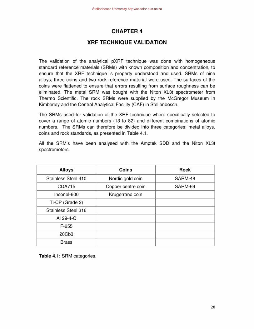
The SRMs used for validation of the XRF technique where specifically selected to

cover a range of atomic numbers (13 to 82) and different combinations of atomic

numbers. The SRMs can therefore be divided into three categories: metal alloys,

coins and rock standards, as presented in Table 4.1.

All the SRM’s have been analysed with the Amptek SDD and the Niton XL3t

spectrometers.

Alloys Coins Rock

Stainless Steel 410 Nordic gold coin SARM-48

CDA715 Copper centre coin SARM-69

Inconel-600 Krugerrand coin

Ti-CP (Grade 2)

Stainless Steel 316

Al 29-4-C

F-255

20Cb3

Brass

Table 4.1: SRM categories.


29

4.1 METAL ALLOY STANDARDS

The results of Stainless Steel 410 [32], CDA715 [33], Inconel-600 [34],

Ti-CP (Grade 2) [35] and Brass alloy are presented in Table 4.2 to Table 4.6. The

other four SRMs were analysed and presented in Appendix F, since they have

similar elemental composition than Stainless Steel 410.

4.1.1 Metal standards results

Table 4.2: Niton XL3t and Amptek SDD measurements for Stainless Steel 410 [32].

The elemental concentrations for both spectrometers were within the known

concentration range as per the SRM certificate of analysis. As discussed in the

method limitation section 3.8, the low atomic number elements cannot be determined

by the PD-FP method, since the method do not use the Compton to Rayleigh

scattering ratio.

Table 4.3: Niton XL3t and Amptek SDD measurements for CDA 715 alloy [33].

Elements Atomic

number

Niton XL3t

Concentration (wt %)

Amptek


SRM


Ni 28 0.25 ± 0.02 0.19 ± 0.01 0.5 max.

Fe 26 87.08 ± 0.06 85.99 ± 0.25 85 – 88.5

Mn 25 0.48 ± 0.03 0.56 ± 0.02 1.0 max.

Cr 24 12.03 ± 0.02 13.26 ± 0.11 11.5 – 13.5

Other Low 0.16 - 0.82 max.

Elements Atomic

number

Niton XL3t Concentration

(wt %)

Amptek SDD

Conctration

(wt %)

SRM known

concentration

(wt %)

Cu 29 68.49 ± 0.06 67.15 ± 0.11 69.5

Ni 28 29.96 ± 0.06 31.27 ± 0.26 29.0 – 33.0

Fe 26 0.58 ± 0.01 0.73 ± 0.03 0.4 – 0.7

Mn 25 0.86 ± 0.01 0.89 ± 0.04 1.0 max.



30

For the CDA715 alloy all the elemental concentrations for both pXRF spectrometers

were in concentration range, as defined by the certificate of analysis of the SRM.

Table 4.4: Niton XL3t and Amptek SDD measurements for Inconel-600 alloy [34].

The concentrations of the other elements, such as Ni, Fe, Mn, Cr and Ti were all

within the known concentration range, as per the SRM certificate of analysis, for both

spectrometers.

The Ti-CP alloy analysed, which is an example of an alloy with one abundant

element, Ti and a very low concentration of Fe.

Table 4.5: Niton XL3t and Amptek SDD measurements for Ti-CP (Grade 2) alloy

[35].

Both the elements and their respective concentration values for the Ti-CP alloy were

within the known concentration range of the SRM.

Elements Atomic number

Niton XL3t Concentration (wt

%)

Amptek SDD

Concentration

(wt%)

SRM known

concentration

(wt %)

Ni 28 74.38 ± 0.061 72.94 ± 0.13 72.0 min.

Fe 26 9.79 ± 0.036 9.75 ± 0.05 6.0 – 10.0

Mn 25 0.29 ± 0.02 0.45 ± 0.01 1.0 max.

Cr 24 14.84 ± 0.04 15.99 ± 0.08 14.0 – 17.0




(wt %)

Amptek SDD

Concentration

(wt%)

SRM known

concentration

(wt %)

Fe 26 0.14 ± 0.01 0.083 ± 0.02 0 – 0.3

Ti 22 99.83 ± 0.03 99.92 ± 0.62 99.3 – 100

Other Low 0.03 - 0.4


31

For pXRF measurements an X-ray generator with a maximum energy of 40 keV was

used, therefore heavier elements are only detected through their L lines. This makes

the spectra analysis more complicated since a variety of lines with different

intensities are observed in the spectrum. Therefore the spectrometer will be

validated for a few high atomic number elements, such as Pb and Au. Pb being part

of the composition of brass were comparatively analysed with the two spectrometers.

The Amptek SDD and concentration results are presented in Figure 4.1 and

Table 4.6, respectively. The Au concentration in the Krugerrand coin will be analysed

in the next section.

Figure 4.1: Amptek SDD spectrometer spectrum for Brass.

Table 4.6: Brass sample concentration results.

The elemental concentrations of all the elements obtained with both spectrometers

are consistent, with a relative low concentration for Pb found. From the results it can

be concluded that the concentration extraction by using the excited L lines is

effective even though the task is more complex.

Element Z number Niton XL3t

concentration (wt %)

Amptek SDD concentration

(wt %)

Pb 82 3.09 ± 0.03 3.63 ± 0.12

Zn 30 38.46 ± 0.12 39.39 ± 0.13

Cu 29 57.56 ± 0.15 56.59 ± 0.16

Co 27 0.025 ± 0.008 0.029 ± 0.012

Fe 26 0.31 ± 0.01 0.39 ± 0.01

V 23 0.021 ± 0.001 0.03 ± 0.02

Other Low 0.53 -

Pb Mα

Ar

V

Fe Kα

Fe Kβ

Co

Cu Kα Zn Kα

Cu K β

Zn Kβ

Pb Lα Pb Lβ

Pb Lɣ


32

4.2 COIN STANDARDS

The Nordic gold coin and a copper centre coin are 50 euro cents and 2 euros respectively. For both coins only the front surface was prepared by flattening the surface. The back of the coin was also measured, to investigate the effect of surface roughness on elemental concentrations. The elemental concentrations are presented in Table 4.7 and Table 4.8. The Krugerrand coin was investigated to determine if the concentration of Au can be

successfully extracted from the L excitation lines. The measured surface of the

Krugerrand coin was not flattened, due to the high monetary value. The elemental

concentration for the Krugerrand coin is presented in Table 4.9.

4.2.1 Coin standards results

Table 4.7: Nordic gold coin concentration results [36].

The elemental concentrations obtained by the Niton XL3t for the Zn, Cu, Al and Sn

elements of the Nordic gold coin, were in line with the expected results.

For the Amptek SDD the Al concentration could however not be determined by the

PD-FP method, since the histogram bin corresponding to the characteristic x-ray

Element Z number

Front Back Back and

Front

Niton XL3t concentration

(wt %)

Amptek SDD Concentration

(wt %)


(wt %)


(wt %)

Known concentration

(wt %)

Sn 50 0.88 ± 0.01 1.84 ± 0.12 0.87 ± 0.01 1.88 ± 0.16 1.0

Nb 41 0.102 ± 0.002 0.254 ± 0.021 0.126 ± 0.005 0.343 ± 0.010 -

Zr 40 0.096 ± 0.005 0.158 ± 0.016 0.117 ± 0.016 0.141 ± 0.011 -

Zn 30 5.03 ± 0.03 5.46 ± 0.05 5.04 ± 0.03 5.49 ± 0.04 5.0

Cu 29 89.32 ± 0.30 87.67 ± 0.17 88.93 ± 0.32 87.59 ± 0.17 89.0

Fe 26 0.047 ± 0.004 0.061 ± 0.004 0.053 ± 0.012 0.061 ± 0.001 -

Mn 25 0.012 ± 0.005 0.118 ± 0.006 0.035 ± 0.004 0.115 ± 0.003 -

Al 13 4.76 ± 0.35 not

determined 5.087 ± 0.34

not

determined 5.0

Other Low 0 - 0.07 - 0.0


33

energy of Al only contain a few counts as can be seen in Amptek SDD spectrum in

Figure 4.2. When analysed by the PD-FP method, it leads to large concentration

errors. For the Niton XL3t the Al concentration could be determined, since the

IOM-FP method uses the information of the Rayleigh and Scatter peaks intensities to

determine the low atomic number concentrations.

There is therefore no means to determine the concentration of Al obtained by the

Amptek SDD and hence only the concentrations of Zn, Sn, Cu and a few low

concentrations elements could be determined. This can be done by forcing the

combined concentrations of Zn, Sn, Cu and the low concentrations elements within

the PD-FP code to account for the low atomic number material, such as Al. This can

however only be done if the concentration of the low atomic number material is

known. In this specific case the assumption is made, since the concentration of the

standard is known. The concentrations of the euro coins are available from KME

database [36]. From Table 4.7 it can be observed that the elemental concentrations

obtained for Zn and Cu are within reasonable values. The forcing of concentration

can be seen as a significant weakness of the PD method, used by the Amptek SDD,

especially for samples were a large part of the weight percentage is from low atomic

number elements.

Figure 4.2: Amptek SDD spectrometer spectrum for Nordic gold

By comparing the elemental concentrations of the front of the coin, which is the

flattened surface, with the elemental concentrations of the back of the coins; it can

be concluded that for pXRF measurements for samples with surface roughness (due

to the engraving on the coin) has little to no impact on the elemental concentrations

for this coin. The results obtained for the Nordic gold coin were in good agreement

Al Ar Sn

Mn Fe

Cu Kα

Zn Kα

Cu K β

Zn Kβ

Zr

Nb

Sn Kα


34

with that of the known elemental concentrations. A few low concentration elements

such as Nb, Zr, Fe and Mn were also measured. However, only the high

concentration elements were indicated in the certificate.

Table 4.8: Copper coin concentration results.

As in the case of the Nordic gold coin, the elemental concentrations of the back and

front of the copper coin compare well, as presented in Table 4.8. Hence there is no

need to account for the engraving in the coins, for the conditions where the

elemental concentration measurement is performed with PXRF.

The second element used for the validation of the pXRF technique (for high atomic

number elements) is Au, as found in the Krugerrand. The Amptek SDD spectrum for

the Krugerrand is presented in Figure 4.3.

Figure 4.3: Amptek SDD spectrometer spectrum for the Krugerrand coin.

Element Z number

Front (flattened surface) Back Back and Front


(wt %)


(wt %)


(wt %)


(wt %)

Known concentration

(wt %)

Zn 30 19.75 ± 0.15 20.58 ± 0.10 19.49 ± 0.07 19.41 ± 0.10 20.0

Cu 29 74.98 ± 0.48 73.99 ± 0.18 74.81 ± 0.20 75.29 ± 0.19 75.0

Ni 28 5.14 ± 0.04 5.43 ± 0.03 5.14 ± 0.02 5.29 ± 0.03 5.0

Other Low 0.13 - 0.56 - 0.0

Au Mα

Ar V

Mn

Cu Au Lα Au Lβ

Au Lɣ

Rb

Sr


35

Table 4.9: XRF analysis results of the Krugerrand coin [37].

The deviation in the concentration for Au, as found in the elemental concentration

results in Table 4.9, is most probably not due to the surface roughness, as

concluded from the results of the euro coins. The overlapping of the Lα lines for Au at

9.71 keV and Lβ for W at 9.67 keV (originating from the X-ray tube) is the most likely

reason. Low concentration elements such as Sr, Rb, Mn and V were also measured.

However, only the high concentration elements were indicated in the certificate.

For the most optimal excitation conditions an X-ray tube energy of greater than the K

absorption edge is required, which would excite the Kα and Kβ lines. Very high energy

portable X-ray tubes are nowadays available which can achieve a maximum energy

of 100 keV. There is however concerns from a radiation protection point of view, as a

result of the high energy.

Element Z number Amptek SDD

Concentration (wt %) Known


Au 79 93.21 ± 0.10 91.67

Sr 38 0.072 ± 0.001 -

Rb 37 0.043 ± 0.010 -

Cu 29 6.79 ± 0.03 8.33

Mn 25 0.021 ± 0.001 -

V 23 0.025 ± 0.004 -

Other Low - 0.0


36

4.3 ROCK STANDARDS

Two rock SRMs, SARM-48 [7] and SARM-69 [8] with high SiO2 content were

analysed. The SARM-48 material comes from the Buffalo Mine, South Africa with

main compounds such as Al2O3, CaO, K2O and SiO2. The material was produced in

a pellet form by the CAF laboratory at Stellenbosch University. The SARM-69 SRM

pellet, which was produced at iThemba Labs, is essentially Late Iron Age pottery

vessels remainings found on the Mkgwareng [38] site, with main compounds such as

Fe2O3, Al2O3 and SiO2.

4.3.1 Rock standard pellet preparation

To ensure homogeneity of the sample the reference material were milled and

pressed into a pellet disk.

The homogeneous pellet disk will ensure that reproducible measurements can be

obtained. This pellet preparation is done with a press capable of creating a pressure

of 20 ton Beckman pressure. The build-up pressure on the sample is initially done

over a 30 second period; once the pressure is reached it is maintained for a further

30 seconds period. The pressure on the sample is then decreased to atmospheric

pressure over a 30 second period. This method results in a pellet with a smooth

surface. The elimination or reduction of the surface contamination was done by

cleaning the sample preparation dye with water, acetone and alcohol before each

pressing process started.

4.3.2 Rock elemental conversion to oxide

The XRF analysis of oxides is performed in an indirect manner since XRF

spectroscopy is only sensitive to elements. Therefore, SiO2 for example is analysed

from the Si element. A conversion factor (as shown in Table 4.10) is used to convert

the concentration of the analysed Si Kα elemental line into the oxide form. The

conversion factor is the molar ratio of silicon and oxygen in SiO2. In Table 4.10 all

the elements and there major oxide phase in rock art paint are indicated.


37

Table 4.10: Stoichiometric factors [39].

4.3.3 Rock standards results

The results for SARM-48 and SARM-69 SRMs obtained by the Niton XL3t and

Amptek SDD are presented in Table 4.11 and Table 4.12.


Element Oxide phase Conversion factor

Si SiO2 2.1393

Ti TiO2 1.6681

Al Al2O3 1.8895

K K2O 1.2046

Ca CaO 1.399

Mg MgO 1.6581

Fe Fe2O3 1.4297

Mn MnO 1.2912

P P2O5 2.2914

Compounds Niton XL3t


Amptek SDD


SRM


Fe2O3 0.57 ± 0.012 0.31 ± 0.01 0.58

Al2O3 9.78 ± 0.14 9.44 ± 0.27 11.24

CaO 7.77 ± 0.12 8.52 ± 0.21 8.90

K2O 5.79 ± 0.08 4.23 ± 0.11 4.26

SiO2 72.47 ± 0.43 74.3 ± 3.0 67.11

MgO 0.95 ± 0.36 0.99 ± 0.28 0.18

TiO2 not detected not detected 0.10

MnO not detected not detected 0.02


38


From the compound concentration of Table 4.11 and Table 4.12, it can be observed

that for the two SRMs the higher atomic number compounds, such as K2O, CaO and

Fe2O3 are in good agreement with that of the known SRM concentrations. For the

lower atomic number compounds, such as MgO and Al2O3 where the concentrations

obtained from the two spectrometers are not that reliable due to the high absorption

of their low energy X-ray K lines.

For SARM-48 the X-ray lines for the compounds TiO2 and MnO were not detected by

either one the spectrometers. This is due to the very low concentrations.

Compounds

Niton XL3t

Concentration

(wt %)

Amptek SDD

Concentration

(wt %)

SRM

(wt %)

Fe2O3 7.71 ± 0.04 5.03 ± 0.02 4.76 – 9.8

Al2O3 14.40 ± 0.20 18.18 ± 2.04 11.12 – 16.49

CaO 2.23 ± 0.03 2.68 ± 0.04 1.33 – 8.19

K2O 1.74 ± 0.03 1.83 ± 0.03 1.28 – 2.78

SiO2 69.78 ± 0.17 70.3 ± 2.3 57.48 – 69.31

MgO not detected 1.0 ± 1.2 1.14 – 2.68

TiO2 0.62 ± 0.01 0.72 ± 0.01 0.57 – 1.02

MnO 0.08 ± 0.01 0.12 ± 0.01 0.08 – 0.19

P2O5 0.27 ± 0.03 0.27 ± 0.11 0.12 – 0.33


39

4.4 XRF TECHNIQUE VALIDATION CONCLUSIONS

Several homogeneous SRMs were used for the validation of the XRF technique,

covering a range of atomic numbers and different combination of atomic numbers.

For all the SRMs the elemental concentrations obtained for both the pXRF

spectrometers were in good agreement with the known concentrations.

For the coin SRMs the front was prepared by flattening the surface. The back of the

coin were also measured to investigate the effect of surface roughness, due to the

engraving on the coin, on elemental concentrations. The elemental concentrations

of both the back and front, for the two SRMs coins, compared well and therefore

there is no need to account for the engraving on coins when elemental concentration

measurement is performed. For the Nordic gold coin the very small Al peak detected

could not be used to determine the Al concentration. Since the PD method used by

the Amptek SDD does not use the C/R calibration to determine the low atomic

number concentrations, as in the case with the IOM-FP method used by the Niton

XL3t. Therefore only the concentrations of Zn and Cu could be determined. This was

done by limiting the combined concentration of Zn and Cu, by assuming the the

known concentration of Al from the certificate, and calculating their concentrations

respectively. This can be seen as a weakness of the PD method, especially for

samples were a large contribution of the weight percentage is from low atomic

number elements.

From the two rock SRMs the compound concentrations for the high atomic number

compounds are in good agreement with that of the known SRM concentration.

However for the low atomic number compounds, such as MgO and Al2O3 the

concentrations obtained using the two spectrometers are not reliable due to the high

absorption of their low energy X-ray K lines.

The Krugerrand coin measured elemental concentrations agreed well the known

SRM elemental concentrations, which demonstrate that the extraction of

concentrations with the use of L lines is effective, even though the task is more

complex. Additionally, the well resolved L X-ray lines by the pXRF detector,

between all the other K X-ray lines, play a vital factor to achieve high accuracy

results for high atomic number elemental concentrations.


40

CHAPTER 5

EXPERIMENTAL RESULTS AND DISCUSSION

5.1 MOUNT AYLIFF ROCK ART FRAGMENT

A rock art fragment from the Mount Ayliff area in Eastern Cape found on the shelter

floor of a cave, which had naturally exfoliated from the bigger rock art painting was

analysed. The fragment is made of sandstone, which mainly consists of SiO2. The

age of the paint on the fragment is estimated to be about 150 years [40] since

scattered remnants of the Bushman still exist in the area. Ten points were

specifically selected, as indicated in Figure 5.1 and analysed in order to obtain the

compound concentrations of each of the points. The ten points included seven paint

points covering a variety of paint colours, two rock varnish points and the back of the

rock. The paint colours ranged from black, shades of brown and shades of red,

where the black paint is due to manganese or charcoal, the red colour is due to iron

oxide and the red-brown colour is due to Hematite (a type of ferrous oxide) [1].

The measurements were performed in consultation with Dr L. Jacobson, the former

Deputy Director of the McGregor Museum in Kimberley.

Figure 5.1: Mount Ayliff rock art fragment with the points that were characterised.

For the analysis, the assumption was made that the rock art fragment consists of

one layer of infinite thickness. Five measurements (obtained by means of the

Amptek SDD and the Niton XL3t spectrometers) were taken at each of the ten points

to improve the statistics and also to avoid anomalies because of grain effects. The

composition analyses are shown in Table 5.1 and Table 5.2 and the Amptek SDD

spectrometer spectrum in Figure 5.2.


41

Figure 5.2: Amptek SDD spectrometer spectrum for the Mount Ayliff rock art fragment (point 1).

Al

Si

S

Ar K

Ca

Ti

Fe


42

5.1.1 Compound concentrations and conclusions

Compounds Al2O3 SiO2 P2O5 S K2O CaO TiO2 Fe2O3

Concentration wt % wt % wt % wt % wt % wt % wt % wt %

Po

int

1

Bla

ck Niton XL3t 0.71 ± 0.11 7.88 ± 0.08 < 0.01 6.89 ± 0.05 0.36 ± 0.01 40.69 ± 0.09 < 0.01 0.78 ± 0.01

Amptek SDD not determined not determined 0.547 ± 0.082 8.338 ± 0.237 1.416 ± 0.015 44.566 ± 0.166 0.699 ± 0.019 2.744 ± 0.019

Po

int

2

Re

d/B

row

n

Niton XL3t 0.89 ± 0.12 11.29 ± 0.09 < 0.01 6.99 ± 0.06 0.38 ± 0.01 35.19 ± 0.08 < 0.01 0.76 ± 0.01


Po

int

3

Re

d/B

row

n

Niton XL3t 2.11 ± 0.10 17.91 ± 0.11 < 0.01 9.19 ± 0.06 0.74 ± 0.02 32.29 ± 0.08 < 0.01 1.08 ± 0.02


Po

int

4

Va

rnis

h Niton XL3t 2.17 ± 0.14 13.86 ± 0.10 < 0.01 9.37 ± 0.06 0.56 ± 0.02 36.88 ± 0.08 < 0.01 0.94 ± 0.01


Po

int

5

Va

rnis

h Niton XL3t 1.75 ± 0.01 11.89 ± 0.10 < 0.01 9.19 ± 0.07 0.38 ± 0.01 41.85 ± 0.09 < 0.01 0.97 ± 0.02


Table 5.1: Compound and element concentration of measured points 1 to 5 for both the Niton XL3t and Amptek SDD

spectrometers.


43

Compounds Al2O3 SiO2 P2O5 S K2O CaO TiO2 Fe2O3

Concentration wt % wt % wt % wt % wt % wt % wt % wt %

Po

int

6

Bla

ck Niton XL3t 1.65 ± 0.15 11.89 ± 0.09 < 0.01 9.01 ± 0.08 0.36 ± 0.01 45.79 ± 0.11 < 0.01 0.73 ± 0.01

Amptek

SDD not determined not determined 2.016 ± 0.013 12.360 ± 0.317 1.13 ± 0.011 37.275 ± 0.171 0.419 ± 0.015 2.728 ± 0.022

Po

int

7

Bla

ck Niton XL3t 1.59 ± 0.15 13.43 ± 0.11 < 0.01 10.39 ± 0.07 0.41 ± 0.01 41.11 ± 0.09 < 0.01 0.88 ± 0.01

Amptek


Po

int

8

Re

d /

Bro

wn

Niton XL3t 0.21 ± 0.11 22.63 ± 0.13 < 0.01 11.88 ± 0.08 0.96 ± 0.02 31.08 ± 0.08 < 0.01 1.18 ± 0.01

Amptek


Po

int

9

Re

d /

Bro

wn

Niton XL3t 0.15 ± 0.15 14.68 ± 0.11 < 0.01 9.59 ± 0.07 0.39 ± 0.01 40.79 ± 0.09 < 0.01 0.66 ± 0.01

Amptek


Ba

ck o

f

rock

Niton XL3t 2.39 ± 0.09 23.58 ± 0.38 < 0.01 not determined 1.29 ± 0.07 13.82 ± 0.12 < 0.01 1.75 ± 0.02

Amptek

SDD not determined not determined 0.377 ± 0.072 0.157 ± 0.033 2.437 ± 0.032 9.250 ±0.050 1.020 ± 0.014 3.589 ± 0.013

Table 5.2: Compound and element concentration of measured points 6 to 9 and back of the rock, for both the Niton XL3t and

Amptek SDD spectrometers.


44

The elemental concentrations of the low atomic number compounds Al2O3 and Si2O

could not be determined by the Amptek SDD PD-FP method, since the PD-FP

method does not use the C/R calibrations to determine low energy compounds.

When the small Si peak in the Figure 5.2 is analysed with the PD-FP method, it

leads to a large concentration error. This is a similar situation as previously

encountered with the Al concentration for the Nordic gold coin analysis, where a

limiting concentration value was used in the PD-FP code for Zn, Sn, Cu and low

concentration elements. A similar approach is used for the low compound and

elemental concentrations Al2O3 and SiO2 of the Mount Ayliff fragment. In order to

compare the concentration of the high atomic number compounds P2O5, S, K2O,

CaO, TiO2 and Fe2O3 the assumption is made that the balance and the

concentrations of Al2O3 and SiO2 for the Niton XL3t is correct and used in an attempt

to obtain the elemental analysis with the PD-FP method.

From the compound concentrations in Table 5.1 and Table 5.2 it can be seen that

the total compound concentration contribution adds up to less than 100 wt %. The

difference or balance is as of a result of elements which cannot be detected such as

H, Na and C (from organic matter) due to the high absorption of their low X-ray

energy in the material. The determination of the balance by the IOM-FP method

(used by the Niton XL3t) is propriety information, but it is likely that a similar method

is used as with the determination of low atomic compound concentrations i.e. where

the information of the Rayleigh and Scatter peaks are used. This ability to calculate the

low atomic number compounds with the IOM-FP method makes it a superior

technique to the PD-FP method, used by the Amptek SDD.

The concentrations of P2O5 and TiO2 compounds obtained with the Amptek SDD

were much higher than the concentrations obtained with the Niton XL3t. Since these

two compound are on the lower (Z = 15 for P) and higher (Z = 22 for Ti) atomic

number compounds range (15 to 26) measured with the Amptek SDD, it is

speculated that the PD-FP method used by the Amptek SDD do not produce

accurate concentrations at the limits of the atomic number ranged measured.

From the results it can be concluded that a uniform coating of high Ca and Si

concentrations is spread across the fragment. Silica rich deposits commonly known

as amorphous silica skins [41] have been observed for certain rock art sites [41]. The

deposits are commonly in the order of ≤ 0.5 mm thick, but can be up to 3 mm. The

mechanism of silica skin formation is however complex, but in the studies carried by

Lovering [42] and Watchman [43] for rock art sites throughout Australia, it was

concluded that the coating formation is due to the slow percolation of ground-waters

through the sandstones. The typical yearly rainfall for the Mount Ayliff region in the

Eastern Cape is about 672 mm per year [44], with leachable elements such as Mg,

K, Ca, Fe and to a lesser extend Al, Si and Mn [1] forming the major constituents of

the layer. The leach of CaO and Si2O from the back to the front of the rock is

illustrated in Figure 5.3, where the points with the same colour were combined to


45

0

5

10

15

20

25

30

35

40

45

We

igh

t p

erc

en

t (w

t%)

Rock

Rock varnish

Red / Brown paint

Black paint

Al2O3 SiO2 S K2O CaO Fe2O3 P2O5 S K2O CaO

obtain an average concentration for each colour. The weathering processes the

account for the account for the extensive removal of the relative mobile elements,

such as Mg, K, Ca and Fe. It appears that this removal process did not happen for

the Mount Ayliff rock fragment, since high CaO concentration was detected.

Weathering processes is complex and depends on many environmental factors and

the material properties of the rock itself [45], such as crystal structure [46], which

result in compositional segregation at the sample surface [47,48,49,50].

Figure 5.3: Elemental compositions by colour and back of the rock

The occurrence of a uniform CaO layer over the rock art was however unexpected. It

was expected that the composition would vary for different colours e.g. the red paint

lines have a high concentration of iron oxide (Fe2O3).

The graphical illustrations of the low and high compound concentrations for the

Niton XL3t are shown in Figure 5.4 and 5.5, Amptek SDD concentrations in Figure

5.6 and 5.7. The concentration of P2O5 and TiO2 for the Niton XL3t is not included

since the concentrations obtained from the Niton XL3t were all below 0.01 weight

percent.

Niton XL3t Amptek SDD


46

0

10

20

30

40

50

Co

nce

ntr

ati

on

(w

t %

)

Compounds

Niton XL3t

Point 1

Point 2

Point 3

Point 4

Point 5

Point 6

Point 7

Point 8

Point 9

SiO2

SCaO

Figure 5.4: Compound and elemental concentrations (wt %) per point for the




0

0.5

1

1.5

2

2.5

Co

nce

ntr

ati

on

(w

t %

)

Compounds

Niton XL3t

Point 1

Point 2

Point 3

Point 4

Point 5

Point 6

Point 7

Point 8

Point 9

Al2O3 K2O Fe2O3


47

0

0.5

1

1.5

2

2.5

3

3.5

Co

nce

ntr

ati

on

(w

t %

)

Compounds

Amptek SDD

Point 1

Point 2

Point 3

Point 4

Point 5

Point 6

Point 7

Point 8

Point 9P2O5





0

10

20

30

40

50C

on

cen

tra

tio

n (

wt

%)

Compounds

Amptek SDD

Point 1

Point 2

Point 3

Point 4

Point 5

Point 6

Point 7

Point 8

Point 9S

CaO


48

5.1.2 Semi-quantitative comparison of the two pXRF spectrometers

For pXRF spectrometer comparison purposes, the compound ratio value which is

determined by dividing the Amptek SDD measured concentration by the measured

concentration value of the Niton XL3t spectrometer, for each point is calculated. With

the concentration ratios determined for S, K2O, CaO and Fe2O3 compounds and

presented in Table 5.3. Since the concentrations of P2O5 and TiO2 for Niton XL3t

were all given below 0.01, the concentration ratios were not calculated. The

compound ratio serves as a means to do a semi-quantitative comparison of the two

pXRF spectrometers. Graphic illustrations of the compound ratio values are

presented in Appendix G.

Table 5.3: Amptek SDD and Niton XL3t compound concentration ratio analysis for S,

K2O, CaO and Fe2O3.

Even though the ratio value could give some insight in the agreement between the

two spectrometers it should not be seen as an absolute were a ratio value of 1 is

good agreement and were any ratio greater or less than 1 is not such good

agreement. Since it should be taken into account that the concentrations for the

Amptek SDD were forced. However limited comparison can be done and with

success for S and CaO compounds, were the average ratio value is approximately 1.

It is speculated that the variation for K2O and Fe2O3 compound concentrations

between the two spectrometers are due to spectra evaluation code inaccuracies for

the heavy Fe (Z=26) compound and light compound K (Z=19) compound.

Element Point

Description S K2O CaO Fe2O3

Point 1 Black 1.21 3.93 1.10 3.52

Point 2 Red / Brown 1.43 2.44 1.19 3.19

Point 3 Red / Brown 1.14 1.00 0.89 1.61

Point 4 Varnish 0.88 1.41 0.92 3.66

Point 5 Varnish 0.75 2.34 0.86 1.88

Point 6 Black 1.37 3.14 0.81 3.74

Point 7 Black 0.98 2.63 0.94 2.16

Point 8 Red / Brown 0.80 0.90 1.02 1.57

Pont 9 Red / Brown 0.92 2.63 0.95 2.77

Average 1.05 2.27 0.97 2.68

Standard

Deviation

0.25 1.00 0.12 0.89


49

5.2 HA KHOTSO ROCK ART FRAGMENT

The rock art fragment in Figure 5.8 was found in cave Ha Khotso in Lesotho. This is

a huge and lengthy shelter with some of the finest rock art in southern Africa. The

cave includes animals painting such as eland, hartebeest, lion, leopard, buck and

guinea fowl. In between these are hunters, dancers and figures of huts - all of which

is done in beautiful styles of red, black and brown shades. The rock fragment

analysed was naturally exfoliated from a larger rock art painting. The fragment is

made of sandstone and its dimensions are about 9 cm2. The colour of the paint on

the rock fragment can be described as a combination of white and yellow i.e. a

cream colour which is covered across the fragment. The Ha Khotso fragment was

analysed by making use of both the pXRF and PIXE [5] techniques, with the area

measured five times. For pXRF, the Amptek SDD with miniature X-ray generator and

for micro-PIXE, the facility at iThemba LABS were used.

Figure 5.8: Ha Khotso rock fragment, with analysed section indicated with a blue

circle.

The Ha Khotso elemental concentrations obtained by PIXE and XRF techniques are

given in Table 5.4 and the Amptek SDD spectrometer spectrum in Figure 5.9.


50

Figure 5.9: Amptek SDD spectrometer spectrum for the front of the Ha Khotso rock fragment.

Si S

Cl

Ar K

Ca

Ti

Mn

Fe

Al


51

5.2.1 Compound concentrations and conclusions

Table 5.4: PIXE and Amptek SDD results for Ha Khotso rock art fragment.

Compounds Na2O MgO Al2O3 SiO2 S Cl K2O CaO TiO2 MnO Fe2O3

Concentration wt % wt % wt % wt % wt % wt % wt % wt % wt % wt % wt %

Ro

ck p

ain

t

(Fro

nt

of

rock

) PIXE 12.71 ± 0.23 3.41 ± 0.04 9.58 ± 0.03 28.29 ± 0.16 12.92 ± 0.07 0.31 ± 0.09 1.31 ± 0.02 28.71 ± 0.33 0.16 ± 0.01 0.15 ± 0.09 1.67 ± 0.03

Amptek

SDD

not

determined

not

determined

not

determined

31.860 ±

1.60

25.921 ±

0.311

0.571 ±

0.069

0.542 ±

0.041

11.239 ±

0.123

0.117 ±

0.009

0.211 ±

0.011

3.854 ±

0.027

Ba

ck o

f ro

ck PIXE

not

determined 1.37 ± 0.04 12.66 ± 0.14 50.84 ± 0.19 18.37 ± 0.15 0.27 ± 0.07 0.91 ± 0.07 13.93 ± 0.05 0.30 ± 0.02 0.41 ± 0.07 0.90 ± 0.01

Amptek

SDD

not

determined

not

determined

not

determined 51.4 ± 2.3

12.897 ±

0.270

0.697 ±

0.077

0.881 ±

0.061

8.524 ±

0.122

0.563 ±

0.023

0.711 ±

0.011 10.98 ± 0.04


52

The graphical illustrations of the compound concentrations for the PIXE and the

Amptek SDD spectrometer are presented in Figure 5.10 and Figure 5.11,

respectively.

Figure 5.10: SiO2, S, CaO and Fe2O3 concentration measurements with the Amptek


Figure 5.11: K2O, TiO2, MnO and Cl concentration measurements with the Amptek


0

10

20

30

40

50

60

Co

nce

ntr

ati

on

(w

t %

)

Compounds

Amptek SDD

PIXE

CaOCaO Fe2O3

Fe2O3

FrontBack

SiO2

0

0.2

0.4

0.6

0.8

1

1.2

1.4

Co

nce

ntr

ati

on

(w

t %

)

Compounds

Amptek SDD

PIXE

K2O

K2OTiO2

TiO2

FrontBack

Cl

S

MnO

SiO2

S CaO

Cl

MnO


53

By comparing the CaO compound concentrations for the back and front of the rock

(for both techniques) a reduction in the compound concentration can be observed

from the front to back of the rock. Therefore the contribution of CaO is a result of the

paint on the Ha Khotso rock fragment. The cream colour of the paint, as can be seen

from Figure 5.8, can thus be correlated to CaO concentration.

The concentration for Na2O, MgO and Al2O3 could not be determined by the Amptek

SDD. From Figure 5.9 it can be seen that Na and Mg was not detected and for Al

only a small peak can be observed, which when analysed with the PD-FP method,

leads to big concentration errors.

The Si2O concentrations from the sandstone rock, compared well for the two

techniques. However several differences in compound concentration for the two

techniques were observed. These differences can be attributed to the fact that the

paint on the fragment is most probably layered and heterogeneous, with the surface

composition having a different composition than the bulk sample. Therefore the

variation in penetration depth due to the difference in energy with which the sample

is bombarded for the two techniques, will result in different compound

concentrations.

Another factor, which could contribute to differences in compound concentrations of

the two techniques, is the distribution of the elements in the analysed region,

together with the difference in spectrometer collimation, 3x3 µm2 and 7 mm2 for the

micro-PIXE and Amptek SDD respectively. Therefore the distribution of the elements

(in the analysis area) were analysed with the micro-PIXE technique. For the larger

beam spot size the measurement will consist of both rock and rock varnish, since the

paint lines are very thin. For the small beam spot size the probability of hitting a

sample grain will increase; which could introduce anomalous concentrations and

therefore not be a true representation of the sample.

5.2.2 PIXE elemental distribution map

Elemental mapping was performed using the Dynamic Analysis [51,52,53] method,

which generate elemental images using K,L and M X-ray lines. The maps are

overlap resolve and background subtracted, with the elements concentration

expressed in weigh percentage. The elemental maps of the two major elements

found in the rock paint Si and Ca are presented in Figure 5.12 and Figure 5.13. The

elemental maps of the other elements found in the rock paint can be seen in

Appendix H.


54

Figure 5.12: Si PIXE elemental composition map for the front of the rock.

Figure 5.13: PIXE element (Ca) composition map for the front of the rock.

From both PIXE elemental maps (1000x250 µm2 area) in Figure 5.12 and

Figure 5.13 the non-uniform distribution of the elements can be seen. This can

definitely result in differences in the compound concentrations for the two

techniques. The rock art paint is typically inhomogeneous and includes cracks, as

demonstrated by the dark area in the centre of the PIXE elemental maps, which

typically occur when the rock art has been exposed to environmental weathering for

long periods of time (typically hundreds of years).


55

Since the Amptek SDD spectrometer is collimated to 7 mm2, the compound

concentrations obtained is essentially a bulk analysis, where the elemental

characterisation is an average of the entire sample volume.

5.3 ROCK ART PAINT THICKNESS PROPERTIES

Even though determination of the thickness of the paint and critical penetration depth

was not part of the objective of the study, estimates of the thickness for rock art paint

was done by J. Huntley with a scanning electron microscopy (SEM), showing that

the thickness can be up to 50 µm [54]. This was measured for the rock art pigment

from the Sydney Basin, which are comparable to the Mount Ayliff and Ha Khotso

sandstone fragments analysed. The critical depth, beyond which any emitted photon

is essentially absorbed and not detected, for light elements such as potassium,

calcium, titanium and iron in silicate rock (representation of sandstone rock) is

estimated to be 30 µm, 35 µm, 50 µm and 170 µm respectively. Since the detection

volume is cone shaped, about half of the contribution of bulk chemical composition is

derived from about 5 µm, 5 µm, 7.5 µm and 50 µm, respectively and for silicon the

penetration depth is estimated to be ~10 µm [55].

5.4 EXPERIMENTAL RESULT CONCLUSIONS

Not all the low atomic number compound concentrations could be determined by the

PD-FP method used by the Amptek SDD. However the higher atomic number

compound concentrations could be obtained, by forcing the combined concentrations

of the high atomic number compounds within the PD-FP code. This can however

only be done if the concentrations of these compounds is known. In the case of the

Mount Ayliff and Ha Khotso fragment this assumption were made, since the

concentrations are obtained from the Niton XL3t.

From the results of the Mount Ayliff fragment concluded that a uniform coating of

high Ca and Si concentrations is spread across the fragment, commonly known as

amorphous silica skins (hydrated amorphous silicon dioxide, SiO2.nH2O). The

mechanism for formation is complex, but it can be concluded that the coating is

formed due to the slow percolation of ground-waters through the orthoquartzites,

with leachable elements such as Mg, K, Ca, Fe and to a lesser extend Al, Si and Mn

[1] forming the major constituents of the layer. Weathering processes then account

for the removal of the relative mobile elements, such as Mg, K, Ca and Fe. It

appears that this removal process did not yet occur for the Mount Ayliff rock

fragment, since high Ca concentration was detected. The occurrence of this layer

over the rock art was however unexpected. It was expected that the composition


56

would vary for different colours. The spectrometer compound concentration ratios for

S and CaO were consistent throughout the analysed points. However, large

variations of K2O and Fe2O3 concentrations were observed between the two

methods, most probably due to the concentration which were not calculated

accurately.

The rock art paint on the Ha Khotso fragment is due to Ca and can be related to the

cream colour of the rock art paint. The Si2O concentrations from the sandstone rock,

compared well for the two techniques. However several differences in compound

concentration for the two techniques can be attributed to the fact that the paint on the

fragment is most probably layered, heterogeneous and non-uniform distribution of

the elements in the analysed region. Additional differences are spectrometer

collimation and X-ray penetration depths.


57

CHAPTER 6

CONCLUSIONS AND RECOMMENDATIONS

6.1 CONCLUSIONS

Homogeneous SRMs of metal alloys, coins and rock standards with a range of

different atomic numbers and known elemental concentrations were used for the

validation of the Amptek SDD and Niton XL3t spectrometers.

The compound concentrations for the metal alloys agreed well with the known

concentrations of the SRMs. From the Nordic gold coin it was learned that the Al

concentration were not determined by the PD method used for the Amptek SDD, it

appears to be an issue with low energy line detection. Therefore in order to

determine the elemental concentration values for Zn and Cu a limiting concentration

needed to be entered into the PD-FP code. Furthermore the roughness due to the

engraving on the coin was not observed to play a significant role in the specific

instance of Nordic gold coin. Very little difference was observed with the two

spectrometers between the smooth and rough surfaces. Measurements on a

Krugerrand coin and brass alloy (with known concentrations) were performed to

demonstrate that the concentration of high atomic number elements, such as Au and

Pb can be accurately measured.

The validation of the SRMs concentrations was very important to advance the

investigation to more complex rock art paintings with heterogeneous and layered

properties.

The characterisation of the rock art fragments, by identifying the elements of the

paint was successfully done. Form the rock art fragment measurements it was found

that the PD-FP method is not effective for low atomic number elements, but with the

assumption that the balance from the Niton XL3t is correct, we have observed some

agreement for the higher atomic numbers compounds. This is therefore by no means

a validation of the PD-FP method but rather show the limitation which is understood

and yield relative good results when applying the assumption.

A uniform layer of high CaO and Si2O compound concentrations were measured.

The slow percolation of ground-waters through the rock, leaching elements such as

Ca, Mg, Fe and K to the surface of the rock [43] is the most likely reason. The

variation of the composition for the different paint colours was hence not observed.

The CaO layer appears to be invisible to the naked eye and possibly acts as a

preserver of the rock art. This may hold the answer to long term conservation of rock

art. A limited comparison of the compound concentrations between the two


58

spectrometers showed that CaO and S compounds compared well. It is speculated

that the variation in concentration for the K2O and Fe2O3 compound is a result of the

PD method not calculating the concentration accurately.

Form the Ha Khotso fragment a reduction in the CaO compound concentration from

the front to the back of the rock was observed with both techniques. This contribution

is a result of the rock art paint and a relation between the high CaO concentration

and the cream colour were established. The difference in compound concentrations

between the PIXE and pXRF technique can be contributed to factors such as the

differences in penetration depth due to the difference in energy with which the

sample is bombarded, the heterogeneous distribution of elements in the analysed

area and difference in spectrometer collimation.

In general high accuracy results can be obtained with pXRF by following a sound

scientific methodology, with specific knowledge and expertise, not only about the

XRF technique, but also about the sample under investigation. Furthermore if

appropriate sample preparation is applied, errors resulting from surface roughness,

particle size effect or heterogeneous of the material can be eliminating or minimised

which will result in high accuracy. Measuring the analysed points 5 times and

obtaining the same results, indicated that the particle size and inhomogeneities did

not have much effect on the compound compositions.


59

6.2 RECOMMENDATIONS

We (as a community) need to integrate the pXRF instruments into archaeological

studies, with the goal to produce accurate results that are comparable across

instruments and manufacturers. This can be done by instrumentation improvements,

characterisation of the effect of rock properties such as grain size, surface texture

and weathering on the elemental concentrations measurements and determining

optimised measurement condition such as the use of a helium environment for low

atomic number compound measurements. The determination of the rock art paint

thickness can also provide useful information, which can improve the accuracy of the

compound concentrations since it can be ensured that the compound concentration

detected is only from the paint layer.

Furthermore, the conservation properties of the CaO layer need to be investigated.

This could possible results in the development of a paint, which can be applied to the

rock art sketches for conservation purposes.


60

BIBLIOGRAPHY

[1] M. Peisach, C.A Pineda and L. Jacobson, Nuclear Analytical Study of Rock

Paintings, Journal of Radioanalytical and Nuclear Chemistry, Articles, Vol. 151, No.1,

221 – 227, 1991.

[2] J.D Lewis-Williams, The rock art of Southern Africa, Cambridge University Press,

Cambridge, England, 1983.

[3] M.J Nuevo, A. Martin Sanchez, C.Oliveira and J. de Oliveira, In situ energy

dispersive X-ray fluorescence analysis of rock art pigment from the ‘Abrigo dos

Gaivoes’ and ‘Igreja dos Mouros’ cave (Portugal), X-ray Spectrometry, Vol 41, Jan

2012.

[4] A. N. Shugar, Portable X-ray Fluorescence and Archaeology: Limitations of the

Instrument and Suggested Methods to achieve desired results, Art Conservation

Department, Buffalo State College, New York.

[5] S.A.E. Johansson, J. L. Campbell, PIXE: A Novel Technique for elemental

analysis, John Wiley & Sons, New York, 1988.

[6] C.G Ryan, D.R. Cousens, S.H Sie and W.L. Griffin, Quantitative analysis of PIXE

spectra in Geoscience applications, Nuclear Instruments and Methods in Physics

Research B49, 271 – 276, 1990.

[7] Certified of Analysis, Fluorspar granite, Reference Material SARM-48, Mintek.

[8] L. Jacobson, W.A. Van der Westhuizen, J. Oosthuysen, SARM-69 Ceramic-1: A

new pottery certified reference material for inter- and intra-laboratory calibration.

[9] G.L Bosco, Development and application of partable, handheld X-ray

fluorescence spectrometers, Trends in Analytical Chemistry, Vol. 45, 121, 2013.

[10] S. Piorek, PPrinciples and applications of man-portable X-ray fluorescence

spectrometry, Trends in analytical chemistry, Vol. 13, no.7, page 281, 1994.


61

[11] N. Craig, R.J. Speakman, R.S Popelka-Filcoff, M.D Glascock, J.D Robertson,

M.S Shackley, M.S Aldenderfer, Comparison of XRF and pXRF for analysis of

archaeological obsidian from southern Peru, Journal of Archaeological Science, 34,

2012 - 2024, 2007.

[12] E. Gliozzo, R. Arletti, L. Cartechini, S. Imberti, W.A Kockelmann, I. Memmi, R.

Rinaldi, R.H Tykot, Non-invasive chemical and phase analysis of Roman bronze

artefacts from Thamusida (Marocco), Applied Radiation and Isotopes, 68, 2246 –

2251, 2010.

[13] Horiba Scientific, XRF Analysis, http://www.horiba.com/scientific/products/x-ray-

fluorescence-analysis/tutorial.

[14] A.C Thompson, D.T Attwood, E.M Gullikson, M.R Howells, J.B Kortright, A.L

Robinson, J.H Underwood, K. Kim, J. Kirz, I. Lindau, P. Pianetta, H. Winick, G.P.

Williams, J.H. Scofield, D.Vaughan, X-ray Data Booklet, X-ray emission energies.

[15] R. E. Van Grieken, A. A. Markowicz, Handbook of X-ray Spectrometry, Second

Edition, Practical Spectroscopy Series Volume 29, 2002, p 47 (Appendix I, Table 4),

p 12 (7), p 219 (5), p 232 (2), p 233 (5), p 233 (6), p 234 (1), p 235 (Figure 22), p 47

(Appendix I, Table 4), p 249 (2), p 247 (4), p 221 (4), p 225 (2), p 230 (2), p 261 (2),

p 306 (3 & 4), p 311 (2), p 265 (1), p 268-269, p 295 (2), p 312, p 312 – 314, p 314.

[16] M.S Shackley, An introduction to x-ray fluorescence spectrometry (XRF)

analysis in archaeology. In M.S. Shackley (ed.), X-Ray Fluorescence, Spectrometry

(XRF) in Geoarchaeology, pp.7–44. New York: Springer, 2011:30.

[17] Thermo Scientific, Using XRF to Sort, Identify and Analyse Scrap Metals and

Alloys in the Recycling Industry with Thermo Scientific Niton XL3t Handheld Alloy

Analyzers.

[18] A.Niculae, P.Lechner, H.Soltau, G.Lutz, L.Struder, C.Fiorini, A.Longoni,

Optimized readout method of silicon drift detectors for high-resolution X-ray

spectrometry, Nuclear Instruments and Methods in Physics Research Section A:

Accelerators, Spectrometers, Detectors and Associated Equipment, Volume 568,

Issue 1, 30, Pages 336 – 342, November 2006.


62

[19] Silicon Drift Detector (SDD) with 125 ev FWHM, Amptek, Figure 12.

[20] Brian Cross, XRF-FP Software Guide v.4.6.0, CrossRoads Scientific, Feb 2010.

[21] V.M. Prozesky, W.J. Prybylowicz, E. van Achterbergh, C.L Churms, C.A.

Pineda, K.A. Springhorn, J.V. Pilcher, C.G. Ryan, J. Kritzinger, H.Schmitt, T.Swart,

The NAC nuclear microprobe facility, Nuclear Instruments and Methods in Physics

Research B 104 (1995) 36 – 42.

[22] N.R. Yoder, IUCF VME Data Acquisition System User Information, Indiana

University Cyclotron Facility, 1994, unpublished.

[23] C.G. Ryan, E. van Achterbergh, C.J. Yeasts, T.T. Win, G. Gripps, Nucl. Instr.

and Meth. B189 (2002) 400.

[24] Instrumentation for PIXE and RBS, IAEA-TECDOC-1190, International Atomic

Energy Agency, December 2000

[25] J.W. Criss, L.S. Birks, Calculation method for fluorescent x-ray spectrometry.

Empirical coefficients versus fundamental parameters, Analytical Chemistry,

Volume 40, page 1080, 1968.

[26] XL3t DTSC’s Portable X-ray Fluorescence Operating Procedure (SOP), SOP,

Appendix A, September 2007.

[27] G.R Lachance, Demystification of Algorithms and Influence Coefficients in

Quantitative XRF Analysis, JCPDS-International Centre for Diffraction Data, 1999.

[28] R. M. Rousseau, Concept of the influence coefficient, The Rigaku Journal, Vol.

18, No.1, 2001.

[29] P.Duvauchell, G.Peix, D.Babot, Effective atomic number in Rayleigh to Compton

scattering ratio, Nuclear Instruments and Mrthods in Physics Research B, 155 ,

1999, 221 – 228.

[30] V.Rackwitz, V.D Hodoroaba, An attempt of exploiting the Compton-to-Rayleigh

Intensity Ration for improved analysis with µXRF and a SEM, Microsc. Microanal 18

(Suppl 2), 2012.


63

[31] M.Donativi, S.Quarta, R. Cesareo, A.Castellano, Rayleigh to Comton ratio with

monochromatic radiation from an X-ray tube (preliminary results), Nuclear

Instruments and Methods in Physics B, 264 (2007), 189 -193.

[32] East Coast Stainless Inc, Stainless steel 410 certificate of analysis.

[33] Hussy copper, CDA 715 certificate of analysis.

[34] Special metals, Inconel 600 certificate of analysis.

[35] Carpenter, Technical Database, Titanium CP Grade 2 certificate of analysis.

[36] KME, Nordic gold coin certificate of analysis.

[37] Birch Gold Group, South African Krugerrand.

[38] T. Maggs, Iron Age communities of the southern Highveld, Natal Museum,

Occasional Publications 2, Pietermaritzburg, 1976.

[39] British Columbia Geological Survey, MINIFILE Coding Manual Version 5.0,

Information Circular 2007-4, Appendix VII - Conversion Factors.

[40] Caves and Cave Art of Lesotho, Southern Africa, Belfry Bulletin No 391/392,

November / December 1980.

[41] A. Watchman, ii. Properties and Dating of Silica Skins associated with Rock Art.

Unpublished PhD Thesis, University of Canberra, Canberra, 1996

[42] J.F Lovering, Epigenetic common opal from the Hawkesbury Sandstone

Formation of the Sydney Basin. Records of the Australian Museum 23:29–32, 1952

[43] A. Watchman, What are silica skins and how are they important in rock art

conservation? Australian Aboriginal Studies (1):21–29, 1990

[44] Mount Ayliff climate; http://www.saexplorer.co.za/south-

africa/climate/mount_ayliff_climate.asp

[45] T. Wells, G. Hancock and J. Fryer, Weathering rates of sandstone in a semi-arid

environment (Hunter Valley, Australia). Environmental Geology 54:1047–1057, 2008.


64

[46] C.R Twidale, Geomorphology: With Special Reference to Australia. Melbourne:

Nelson, 1968:136–137.

[47] N.Cook, I. Davidson, S. Sutton, Why are so many ancient rock paintings

red? Australian Aboriginal Studies (1):30–33, 1990.

[48] P.J Potts, Introduction, analytical instrumentation and application overview.

In P.J. Potts and M. West (eds), Portable X-Ray Fluorescence Spectrometry:

Capabilities for In Situ Analysis, pp.1–12. Cambridge: Royal Society of Chemistry

Publishing, 2008.

[49] M.A Smith, B. Fankhauser, M. Jercher, The changing provenance of red ochre

at Puritjarra rock shelter, Central Australia: Late Pleistocene to present.

Proceedings of the Prehistoric Society 64:275–292, 1998.

[50] O. Williams-Thorpe, The application of portable x-ray fluorescence analysis to

archaeological lithic provenancing. In P.J. Potts and M. West (eds), Portable X-Ray

Fluorescence Spectrometry: Capabilities for In Situ Analysis, pp.174–205.

Cambridge: Royal Society of Chemistry Publishing, 2008.

[51] C.G. Ryan, Quantitative trace element imaging using PIXE and the nuclear

microprobe, Int. J. Imag. Syst. Tech. 11 (2000) 219–230.

[52] C.G. Ryan, D.N. Jamieson, Dynamic analysis - on-line quantitative PIXE

microanalysis and its use in overlap-resolved elemental mapping, Nucl.

Instrum. Methods Phys. Res. B 77 (1993) 203–214.

[53] C.G. Ryan, D.N. Jamieson, C.L. Churms, J.V. Pilcher, A new method for on-line

true-elemental imaging using PIXE and the proton microprobe, Nucl. Instrum.

Methods Phys. Res. B 104 (1995) 157–165.

[54] J. Huntley, Taphonomy or paint recipe: In situ portable X-ray fluorescence

analysis of two anthropomorphic motifs from the Woronora Plateau, New South

Wales.


65

[55] P.J Potts, O. Williams-Thorpe, P.C. Webb, The bulk analysis of silicate rocks by

portable x-ray fluorescence: Effect of sample mineralogy in relation to the size of the

excited volume, The Journal of Geostandards and Geoanalysis 21(1):29–41, 1997.

[56] Digital Pulse Processor, DP5, Amptek.

[57] Stainless steel 316 product data sheet, AK Steel.

[58] Al 29-4-C alloy technical data sheet, ATI.

[59] F-255 alloy data sheet, Corrosion Materials.

[60] 20Cb3 alloy specification, Alloy Wire International.


66

APPENDIX A:

DIGITAL PULSE PROCESSOR [56]

The function of the digital pulse processor is to digitize the preamplifier output,

applies real-time digital processing to the signal, detects the peak amplitude and bins

this value in its histrogramming memory to generate an energy spectrum. The

proses steps is illustrated in Figure A.1 for the DP5 used by the Amptek SDD.

Figure A.1: Block diagram of the Amptek SDD digital pulse processor DP5 [56].

The analog prefilter receives its input from the output of a charge sensitive

preamplifier. The main function of this circuit are applying the appropriate gain and

offset to utilize the dynamic range of the ADC, and carrying out some filtering and

pulse shaping functions to optimize the digitization.

ADC digitizes the output of the analog prefilter at a 20 to 80 MHz rate then sends it in

real time to the digital pulse shaper. Two parallel signal processing paths inside the

Digital Pulse Shaper receives the output from the ADC, which is being processed

continuously by using pipeline architecture to generate a real time shapping

amplifier. The shaped pulse is a purely digital entity. There are two parallel signal

processing paths inside the DPP, the ‘fast’ and the ‘slow’ channels, optimized to

obtain different data about the incoming pulse train. The ‘slow’ channel, has a long

shaping time constant, is optimized to obtain accurate pulse heights. The peak value

for each pulse in the slow channel, a single digital quantity, is the primary output of

the pulse shaper. The ‘fast’ channel is optimized to obtain timing information:

detecting pulses which overlap in the slow channel, measuring the incoming count

rate, measuring pulse risetimes etc. The DP5 from Amptek SDD, uses trapezoidal

pulse shaping, which offers high energy resolution.

Detector &

Preamplifier

Analog

Prefilter

ADC Digital Pulse

Shaper

Histogram

Logic

Microcontroller

& Interface

Computer,

USB

Pulse Selection

Logic

Power

Supply

+ 5 V DC

Aux I/O


67

The pulse selection logic rejects pulses for which an accurate measurement cannot

be made. It includes pileup rejection, risetime discrimination logic for an external

gating signal etc. At high count rates, the DP5 has both better pileup reject and

higher throughput than a traditional, analog shaping amplifier.

Histogramming memory operates as in a traditional MCA. When a pulse occurs with

a particular peak value, a counter in a corresponding memory location is

incremented. The result is a histogram, an array containing, in each cell, the number

of events with the corresponding peak values. This energy spectrum is the primary

output of the DP5.

The DP5 includes hardware and software to interface between these various

functions and the user’s computer. The main function is however to transmit the

spectrum to the user. Alternatively it controls the data acquisition, by starting and

stopping the processing and by clearing the histogram memory. It also controls

certain aspects of the analog and digital shaping, by setting the analog gain or pulse

shaping time.


68

APPENDIX B:

PD-FP TFR INPUT FILE

B.1 LAYER TABLE

1

"Thick","Type","Thick.Error","Thick.Units","Density","Fixed","Norm.Flag","Total"

0,"Bulk",0,"mg/cm2",0,"No","On",100

B.2 SAMPLE TABLE

15

"Layer","Component","Type"

1,"Si","Calc"

1,"Fe","Calc"

1,"Ca","Calc "

1,"Ti","Calc "

1,"P","Calc"


69

1,"Mn","Calc"

1,"K","Calc"

1,"C","Calc"

1,"N","Calc"

1,"S","Calc"

1,"Ni","Calc"

1,"Zr","Calc”

1,"Sr","Calc"

1,"Rb","Calc"

1,"Al","Calc"


70

B.3 ELEMENT TABLE

15

"Elmt","Line","Cond.Code","Intensity","Int.Err","Back.Int","Back.Err","n-

sigma","Type","Int.Method","Ratio Method","ROI

Low","High","Chi2","Quant.Meth.","Conc","Error","MDL","Atomic%","TCC","TCC

Error","CC","CC2","CC3","LowMT","HighMT"

"C ","Ka",0,0,0,0,0,0,"ConcThresh","Gaussian","None",0,0,0,"None",30,0,0,41.70259,0,0,0,0,0,0,0

"N ","Ka",0,0,0,0,0,0,"ConcThresh","Gaussian","None",0,0,0,"None",30,0,0,35.76014,0,0,0,0,0,0,0

"Al","Ka",0,2.616379,.1811982,0,0,0,"ConcThresh","Gaussian","None",1.410023,1.56298,1.433366,"None"

,1,0,0,.6187962,0,0,0,0,0,0,0

"Si","Ka",1,0,0,0,0,0,"ConcThresh","Gaussian","None",1.661607,1.817797,1.160309,"FP",0,0,0,0,0,0,0,0,0,

0,0

"P

","Ka",1,0,0,0,0,0,"ConcThresh","Gaussian","None",1.933303,2.093103,.3202974,"FP",0,0,0,0,0,0,0,0,0,0,0

"S

","Ka",0,37.40493,.6851221,0,0,0,"ConcThresh","Gaussian","None",2.225513,2.388894,33.37701,"None",.

5,0,0,.260334,0,0,0,0,0,0,0

"K


71

","Ka",0,24.44316,.5382372,0,0,0,"ConcThresh","Gaussian","None",3.224485,3.400429,7.140087,"None",.

9997905,0,0,.4269381,0,0,0,0,0,0,0

"Ca","Ka",0,911.4768,3.286759,0,0,0,"ConcThresh","Gaussian","None",3.5995,3.780319,288.5868,"None",

25.7606,0,0,10.73147,0,0,0,0,0,0,0

"Ti","Ka",0,10.91994,.3597536,0,0,0,"ConcThresh","Gaussian","None",4.412144,4.603585,4.966556,"None

",.2616434,0,0,9.126124E-02,0,0,0,0,0,0,0

"Mn","Ka",0,3.50993,.2039596,0,0,0,"ConcThresh","Gaussian","None",5.788303,5.998248,1.692336,"None

",2.499507E-02,0,0,7.596178E-03,0,0,0,0,0,0,0

"Fe","Ka",0,220.5539,1.616786,0,0,0,"ConcThresh","Gaussian","None",6.289094,6.505564,87.97106,"Non

e",1.134782,0,0,.3392659,0,0,0,0,0,0,0

"Ni","Ka",0,3.54477,.2049694,0,0,0,"ConcThresh","Gaussian","None",7.354451,7.584724,6.17233,"None",

1.098668E-02,0,0,3.125295E-03,0,0,0,0,0,0,0

"Rb","Ka",0,4.776441,.2379289,0,0,0,"ConcThresh","Gaussian","None",13.20637,13.52494,.4070899,"Non

e",2.823822E-02,0,0,5.516309E-03,0,0,0,0,0,0,0

"Sr","Ka",0,38.8594,.6786457,0,0,0,"ConcThresh","Gaussian","None",13.96578,14.29735,8.155778,"None"

,.2525188,0,0,4.811708E-02,0,0,0,0,0,0,0

"Zr","Ka",0,3.49832,.203622,0,0,0,"ConcThresh","Gaussian","None",15.55333,15.91295,3.023425,"None",

2.644894E-02,0,0,4.840742E-03,0,0,0,0,0,0,0


72

B.4 CONDITION TABLE (ACQUIRE / PROCESSING PARAMETERS)

1

"Target","Filter","Thick.(um)","kV","uA","Det.Type","Det.Filter","Thick.(um)","Atmos","Preset

Time","Acq.Time","Smooths","Escape","Sum","Backgrd.","Blank","Blank File"

"C/R Ratio","Compton(c/s)","ROI-Low","ROI-High","Rayleigh(c/s)","ROI-Low","ROI-High","Monitor"

"W ","None",1.5,40,5,"Si pin","None",300,"Air",0,318.752,2,"Yes","Yes","Auto","No",""

"No",0,0,0,0,0,0,0

B.5 DETECTOR PARAMETERS

"Det.Z","FWHM(eV)","Type","Model","Area(mm2)","Coll.(mm)","Thk.(mm)","Ice(nm)"

14,165,2,0,7,5,.3,0

"Contact(Z)","Cont.Thk(nm)","DL(um)","Azimuth","DetAngle","Alpha","Pressure(Torr)"

79,0,0,0,45,0,0


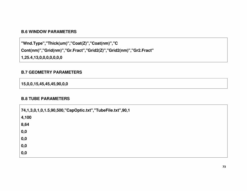
73

B.6 WINDOW PARAMETERS

"Wnd.Type","Thick(um)","Coat(Z)","Coat(nm)","C

Cont(nm)","Grid(nm)","Gr.Fract","Grid2(Z)","Grid2(nm)","Gr2.Fract"

1,25.4,13,0,0,0,0,0,0,0

B.7 GEOMETRY PARAMETERS

15,0,0,15,45,45,45,90,0,0

B.8 TUBE PARAMETERS

74,1,3,0,1,0,1.5,90,500,"CapOptic.txt","TubeFile.txt",90,1

4,100

8,64

0,0

0,0

0,0

0,0


74

0,0

0,0

0,0

0,0

0,0

0,0

0,0

0,0

0,0

0,0

0,0

0,0

0,0

0,0

0,0

0,0

0,0

0,0


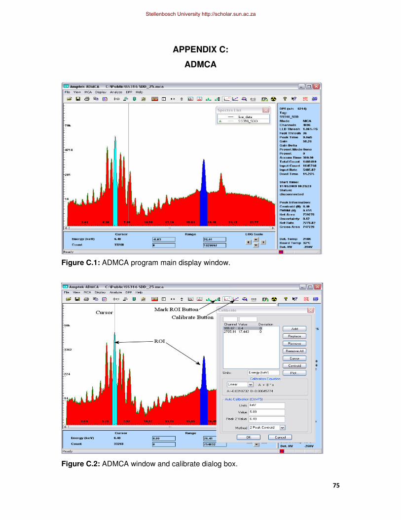
75

APPENDIX C:

ADMCA

Figure C.1: ADMCA program main display window.

Figure C.2: ADMCA window and calibrate dialog box.


76

APPENDIX D:

LEVERBERG-MARQUARDT ALGORITHM

The gradient and first-order expansion form the basis of the popular Leverberg-

Marquardt algorithm.

D.1 Gradient method [15]

For the gradient method the fitting function y = y(x,a) and <) defined as a function of

m parameters aj

<) = <)(:) = ∑ �=7 [,- − ,(A- , :)])>-2� (D.1)

The gradient of <) in the m-dimensional parameter space is given by

∇<) =∑ +O+�P1 Q (D.2)

where j is the unit vector along the axis j and the components of the gradient are

given by

ROR�P =−2∑ �

=7- [,- − ,(A- , :)] R6R�P (D.3)

where T1 is defined as

T1 = − �) RO

R�P (D.4)

The gradient gives the direction in which <) increases most rapidly. A method to

locate the minimum can thus be developed on this basis. Given the set of

parameters aj , a new set of parameters a’j is calculated, for all j simultaneously:

:1U = :1 + ∆aXT1 (D.5)

which follows the direction of steepest descent and guarantees a decrease of <) (at

least if the appropriate step sizes ∆aXare taken).

The gradient method works well away from the minimum, but near the minimum, the

gradient becomes to small (or even zero) and thus is not a good method to use on its

own.


77

D.2 First-order Expansion [15]

By writing the fitting function y(xi, a) as a first-order Taylor expansion of the

parameters aj around y0

,(A, :) = ,�(A, :) +∑ R6�(Y,�)R�P1 Z:1 (D.6)

We obtain an approximation to the fitting function which is linear in the parameter

increments Z:1. ,�(A, :) is the value of the fitting function for some initial set of

parameters a. By inserting equation D.6 into equation D.1 the <) function can be

express as

<) = ∑ �=7- [,- − ,�(A- , :) −∑ R6�(Y7,�)

R�P Z:11 \) (D.7)

The linear least squares method can now be used to find parameters Z:1 so that <) will be minimal. Fitting the difference ,-U = ,- − ,�(A- , :) with the derivatives as

variables and the increments Z:1 as unknowns.

As defined in the linear least squares fitting section previously:

;1 = R6�(Y7)R�P (D.8)

T1 = ∑ �=7

>-2� [,- − ,�(A-)] R6](Y7)R�P (D.9)

1̂_ = ∑ �=7

>-2� R6�(Y7)R�P R6�(Y7)R�` (D.10)

Defining a set of m normal equations in the unknowns Z:1, T = ^Z^ (D.11)

with solution

Z:1 =∑ ^3�1__2� T_ (D.12)

thus

T1 = − �) RO�

R�` (D.13)

and the component of the gradient of <) at the point of expansion

1̂_ ≈ �) RO�R�Pb�` (D.14)

Thus, 1̂_, is the first-order approximation to the curvature matrix whose inverse is

the error matrix.


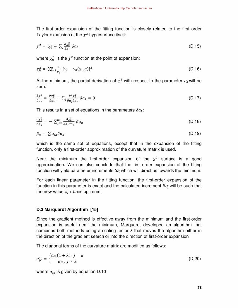
78

The first-order expansion of the fitting function is closely related to the first order

Taylor expansion of the <) hypersurface itself:

<) = <�) +∑ RO�R�P1 Z:1 (D.15)

where <�) is the <) function at the point of expansion:

<�) = ∑ �=7

>-2� [,- − ,�(A-, :)]) (D.16)

At the minimum, the partial derivation of <) with respect to the parameter ak will be

zero:

ROR�` = RO�

R�` +∑ RO�

R�PR�`1 Z:_ = 0 (D.17)

This results in a set of equations in the parameters Z:_:

RO�R�` =−∑ RO�

R�PR�`12� Z:_ (D.18)

T_ = ∑ 1̂_Z:_ (D.19)

which is the same set of equations, except that in the expansion of the fitting

function, only a first-order approximation of the curvature matrix is used.

Near the minimum the first-order expansion of the <) surface is a good

approximation. We can also conclude that the first-order expansion of the fitting

function will yield parameter increments δaj which will direct us towards the minimum.

For each linear parameter in the fitting function, the first-order expansion of the

function in this parameter is exact and the calculated increment δaj will be such that

the new value aj + δaj is optimum.

D.3 Marquardt Algorithm [15]

Since the gradient method is effective away from the minimum and the first-order

expansion is useful near the minimum, Marquardt developed an algorithm that

combines both methods using a scaling factor λ that moves the algorithm either in

the direction of the gradient search or into the direction of first-order expansion

The diagonal terms of the curvature matrix are modified as follows:

1̂_U = d:1_(1 + f), g = h1̂_ , g ≠ h (D.20)

where 1̂_ is given by equation D.10


79

1̂_ = ∑ �=7

>-2� R6�(Y7)R�P R6�(Y7)R�` (D.21)

and the matrix equation to be solved for the increments δ aj is

T1 = ∑ 1̂_U Z:__ (D.22)

When λ is very large (λ >> 1), the diagonal elements of α dominate and the equation

reduce to

T1 ≈ 1̂1U Z:_ (D.23)

or

Z:_ ≈ �jPPk T1 ≈

�jPPk

+O+�` (D.24)

which is the gradient, scaled by a factor 1̂1U .

For small values of λ (λ << 1) the solution is very close to first-order expansion.

The algorithm proceeds as follows:

1. Given some initial values of the parameters aj , evaluate <) =<)(:) and

initialize λ = 0.0001

2. Compute β and α matrices

3. Modify the diagonal elements 1̂1U = 1̂1 + f and compute δa

4. If χ)(m + δm) ≥ χ)(m)increase λ by a factor of 10 and repeat Step 3;

If χ)(m + δm) < χ)(m)decrease λ by a factor of 10

accept new parameters estimates m ← m + Zm and repeat Step 2.

The algorithm thus performs two loops: the inner loop incrementing λ until χ) starts

to decrease and the outer loop calculating successively better approximations to the

optimum values of the parameters. The outer loop can be stopped when χ) decreases by a negligible absolute or relative amount. Once the minimum is

reached, the diagonal elements are an estimate of the uncertainty in the fitting

parameters just as in the case of linear least squares: r�1) = 1̂13� which is equal to (αjj

’ )-1 providing the scaling factor λ is much smaller than 1.


80

APPENDIX E:

FP EQUATION

By dividing the numerator and denominator of the FP method (equation 4.11) by �-∗ gives the expression [28]:

I- = s(7) 7 7/∑ t7P PP (E.1)

which leads to the algorithm

K- = u-vK- +∑ �-1K11 w (E.2)

where u- = s7s(7) and Tertian proposed a matrix effect in �-1coefficient

�-1 = t7P∗ 3 7x7P�/(�3 7)x7P with �-1∗ coefficient relating the absorption effect, while ℎ-1 relates the

enhancement effect

To eliminate the term K- on both sides of equation (E.2), Lachance and Traill

proposed the expression

K- = u-v1 + ∑ :-1JK11 w (E.3)

where :-1J = yLP∗3L7∗L7∗ z = {�-1J − 1| and usable for theoretical procedures of monochromatic excitation source,

absorption and binary element system.

Criss and Birks [25] proposed that the integrals be replaced by a finite summation

over the number of discrete effective wavelength intervals and furthermore that the

experimentally measured of the X-ray tube spectra should be used as excitation

sources for theoretical calculations. This gave the ‘Fundamental Parameter

Approach’ with general form:

I- + }- = ~-K- ∑ ��L7��D�-�>�(�J (�Hℎ:H��5�H��5) (E.4)

From the general form, the concept of theoretical influence coefficients was

developed by de Jongh, Rousseau, Lachance and Claisse with the expression [27]

I(-)K- = I- + }- +∑ �-1K1 −∑ #-1K111 (E.5).


81

APPENDIX F:

NITON XL3t AND AMPTEK SDD FOR IRON (Fe) ALLOY METALS

Table F.1: Niton XL3t and Amptek SDD measurements for Stainless Steel 316 [57].

Table F.2: Niton XL3t and Amptek SDD measurements for Al 29-4-C alloy [58].

Elements Atomic

number

Niton XL3t


Amptek

Conctration (wt %)

SRM

Concentration (wt%)

Mo 42 2.19 ± 0.01 3.04 ± 0.03 2.0 – 3.0

Ni 28 11.16 ± 0.06 9.97 ± 0.07 10.0 – 14.0

Fe 26 67.68 ± 0.07 66.88 ± 0.17 63.0 – 72.0

Mn 25 1.84 ± 0.04 1.62 ± 0.02 2.0 max.

Cr 24 16.84 ± 0.04 18.08 ± 0.07 16.0 – 18.0




(wt %)

Amptek

Conctration

(wt %)

SRM

Concentration

(wt %)

Mo 42 3.85 ± 0.011 3.74 ± 1.44 4.0

Ni 28 0.23 ± 0.02 0.19 ± 0.03 0.3

Fe 26 66.08 ± 0.08 64.94 ± 0.51 65.2 - 66.2

Mn 25 0.34 ± 0.04 0.49 ± 0.06 0.5

Cr 24 28.47 ± 0.06 30.36 ± 0.30 29.0



82

Table F.3: Niton XL3t and Amptek SDD measurements for F-255 alloy [59].

Table F.4: Niton XL3t and Amptek SDD measurements for 20Cb3 alloy [60].

Elements Atomic

number


(wt %)

Amptek

Conctration

(wt %)

SRM

Concntration

(wt %)

Mo 42 3.73 ± 0.01 3.49 ± 0.10 2.9 – 3.9

Cu 29 1.45 ± 0.02 1.44 ± 0.12 1.5 – 2.5

Ni 28 5.76 ± 0.05 5.94 ± 0.24 4.5 – 6.5

Fe 26 63.48 ± 0.08 62.16 ± 0.66 58.6 – 67.1

Mn 25 0.96 ± 0.04 1.28 ± 0.08 1.5 max.

Cr 24 24.37 ± 0.05 25.92 ± 0.31 24.0 – 27.0

Other Low 0.25 - 1.36

Elements Atomic

number

Niton XL3t Concentration (wt %)

Amptek Conctration

(wt %)

SRM

Concentration

(wt %)

Mo 42 2.17 ± 0.01 3.74 ± 1.24 2.0 – 3.0

Cu 29 3.09 ± 0.03 3.13 ± 0.12 3.0 – 4.0

Ni 28 33.07 ± 0.07 33.35 ± 0.34 32.0 – 38

Fe 26 40.96 ± 0.06 39.38 ± 0.32 31.0 - 43.0

Cr 24 19.39 ± 0.04 19.38 ± 0.20 19.0 – 21.0


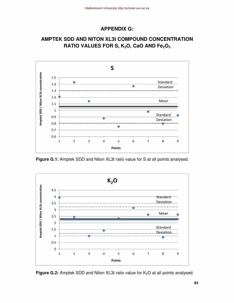
83

0.6

0.7

0.8

0.9

1

1.1

1.2

1.3

1.4

1.5

1 2 3 4 5 6 7 8 9

Am

pte

k S

DD

/ N

ito

n X

L3t

con

cen

tra

tio

n

Points

S

Mean

Standard

Deviation

Standard

Deviation

APPENDIX G:

AMPTEK SDD AND NITON XL3t COMPOUND CONCENTRATION

RATIO VALUES FOR S, K2O, CaO AND Fe2O3

Figure G.1: Amptek SDD and Niton XL3t ratio value for S at all points analysed.

Figure G.2: Amptek SDD and Niton XL3t ratio value for K2O at all points analysed.

0

0.5

1

1.5

2

2.5

3

3.5

4

4.5

1 2 3 4 5 6 7 8 9

Am

pte

k S

DD

/ N

ito

n X

L3t

con

cen

tra

tio

n

Points

K2O

Mean

Standard

Deviation

Standard

Deviation


84

Figure G.3: Amptek SDD and Niton XL3t ratio value for CaO at all points analysed.

Figure G.4: Amptek SDD and Niton XL3t ratio value for Fe2O3 at all points analysed.

0.6

0.7

0.8

0.9

1

1.1

1.2

1.3

1 2 3 4 5 6 7 8 9

Am

pte

k S

DD

/ N

ito

n X

L3t

con

cen

tra

tio

n

Points

CaO

Standard

Deviation

Mean

Standard

Deviation

1.4

1.9

2.4

2.9

3.4

3.9

1 2 3 4 5 6 7 8 9

Am

pte

k S

DD

/ N

ito

n X

L3t

con

cen

tra

tio

n

Points

Fe2O3

Mean

Standard

Deviation

Standard

Deviation


85

APPENDIX H:

ELEMENTAL MAPS OF THE HA KHOTSO ROCK OBTAINED WITH

THE PIXE METHOD

Figure H.1: Mg PIXE elemental composition map for the front of the rock.

Figure H.2: S PIXE elemental composition map for the front of the rock.


86

Figure H.3: K PIXE elemental composition map for the front of the rock.

Figure H.4: Fe PIXE elemental composition map for the front of the rock.


Documents

Portable X-ray Fluorescence and Nuclear Microscopy Techniques