Embed Size (px)
Citation preview

Principled Assessment of Population Structure in Models of Language ChangeJordan Kodner & Christopher Cerezo FalcoUniversity of Pennsylvania
DiGS 19, September 8, 2017 Stellenbosch University
Slides Available Here:
ling.upenn.edu/~jkodner

Outline
● Frameworks for Population-Level Change● Description of our Framework● Population Size and Assumptions about the Grammar● Realistic Networks and the Path of Change

Modeling Population-Level Change
Why Simulate Change?
● We have lots of data on historical change and change in progress - evidence

Why Simulate Change?
● We have lots of data on historical change and change in progress - evidence● We have logically derived theories of change - evidence

Why Simulate Change?
● We have lots of data on historical change and change in progress - evidence● We have logically derived theories of change - evidence● But we cannot test large scale language change in the lab - missing evidence
Why Simulate Change?
● We have lots of data on historical change and change in progress - evidence● We have logically derived theories of change - evidence● But we cannot test large scale language change in the lab - missing evidence
It would be nice to test cause an effect directly.

Why Simulate Change?
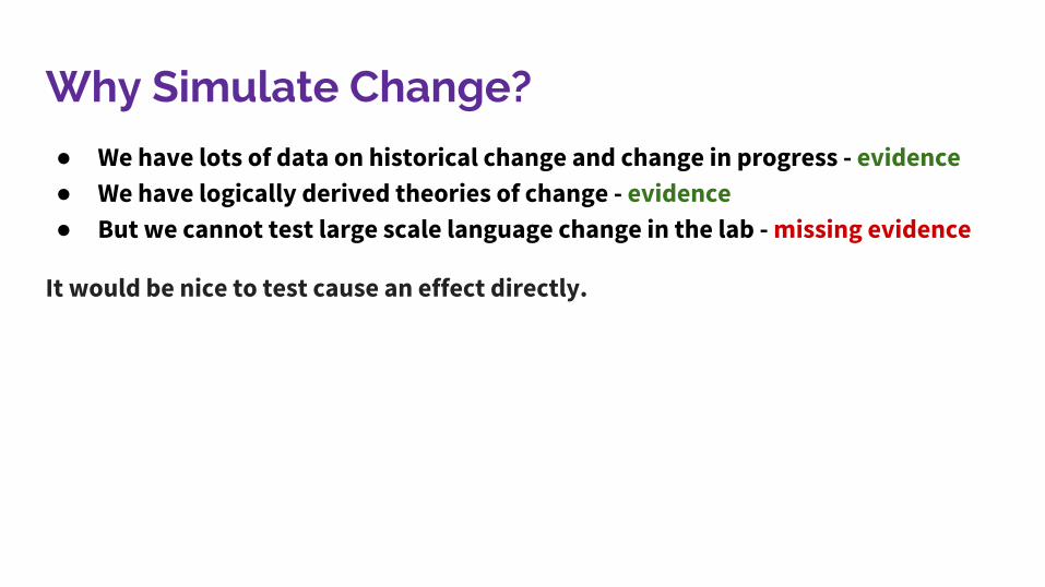
● We have lots of data on historical change and change in progress - evidence● We have logically derived theories of change - evidence● But we cannot test large scale language change in the lab - missing evidence
It would be nice to test cause an effect directly.
Simulation provides that outlet.
A useful tool in computational biology, epidemiology, computational social sciences, etc.

Three Classes of Framework
1. Concrete Frameworks2. Network Frameworks3. Algebraic Frameworks

Three Classes of Framework
1. Concrete Frameworks● Individual agents on a grid moving randomly and interacting● e.g., Harrison et al. 2002, Satterfield 2001, Schulze et al. 2008, Stanford &
Kenny 2013

Three Classes of Framework
1. Concrete Frameworks● Individual agents on a grid moving randomly and interacting● e.g., Harrison et al. 2002, Satterfield 2001, Schulze et al. 2008, Stanford &
Kenny 2013+ Gradient interaction probability for free+ Diffusion is straightforward- Not a lot of control over the network- Thousands of degrees of freedom -> should run many many times -> slow- Unclear how to include a learning model

Three Classes of Framework
1. Concrete Frameworks2. Network Frameworks
● Speakers are nodes in a graph, edges are possibility of interaction● e.g., Baxter et al. 2006, Baxter et al. 2009, Blythe & Croft 2012, Fagyal et
al. 2010, Minett & Wang 2008, Kauhanen 2016
Three Classes of Framework
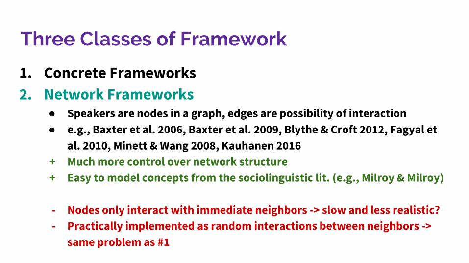
1. Concrete Frameworks2. Network Frameworks
● Speakers are nodes in a graph, edges are possibility of interaction● e.g., Baxter et al. 2006, Baxter et al. 2009, Blythe & Croft 2012, Fagyal et
al. 2010, Minett & Wang 2008, Kauhanen 2016+ Much more control over network structure+ Easy to model concepts from the sociolinguistic lit. (e.g., Milroy & Milroy)
- Nodes only interact with immediate neighbors -> slow and less realistic?- Practically implemented as random interactions between neighbors ->
same problem as #1

Three Classes of Framework
1. Concrete Frameworks2. Network Frameworks3. Algebraic Frameworks
● Expected outcome of interactions in a perfectly mixed population is calculated analytically
● Abrams & Stroganz 2003, Baxter et al. 2006, Minett & Wang 2008, Niyogi & Berwick 1997, Niyogi & Berwick 2009

Three Classes of Framework
1. Concrete Frameworks2. Network Frameworks3. Algebraic Frameworks
● Expected outcome of interactions in a perfectly mixed population is calculated analytically
● Abrams & Stroganz 2003, Baxter et al. 2006, Minett & Wang 2008, Niyogi & Berwick 1997, Niyogi & Berwick 2009
+ Less reliance on random processes -> faster and more direct+ Clear how to insert learning models into the framework- No network structure! Always implemented over perfectly mixed
populations

Our Framework
Best of Both Worlds
● An algebraic model operating on network graphs

Best of Both Worlds
● An algebraic model operating on network graphs○ No random process in the core algorithm○ Fast and efficient

Best of Both Worlds
● An algebraic model operating on network graphs○ No random process in the core algorithm○ Fast and efficient○ Models language change in social structures

Vocabulary for this Talk
Different research traditions, Different vocabularies
L: That which is transmittedLanguage ≈ Variety ≈ *Lect ≈ E-Language
G: That which generates/describes/distinguishes LThat which is learned/influenced by LGrammar ≈ Variant ≈ I-Language

The Model
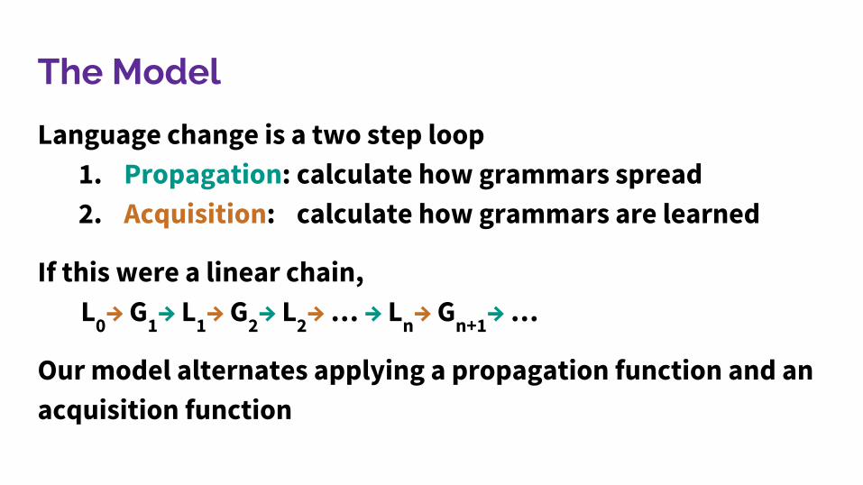
Language change is a two step loop1. Propagation: calculate how grammars spread2. Acquisition: calculate how grammars are learned

The Model
Language change is a two step loop1. Propagation: calculate how grammars spread2. Acquisition: calculate how grammars are learned
If this were a linear chain,L0→ G1→ L1→ G2→ L2→ … → Ln→ Gn+1→ …
The Model
Language change is a two step loop1. Propagation: calculate how grammars spread2. Acquisition: calculate how grammars are learned
If this were a linear chain,L0→ G1→ L1→ G2→ L2→ … → Ln→ Gn+1→ …
Our model alternates applying a propagation function and an acquisition function

Formal Description
[ REDACTED ]
Propagation
Network Structure
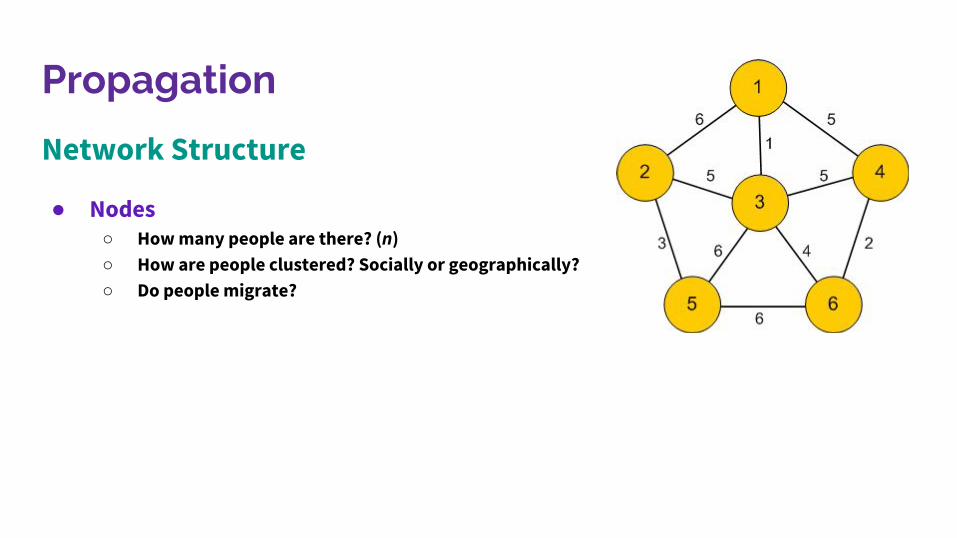
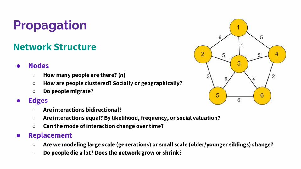
● Nodes○ How many people are there? (n)○ How are people clustered? Socially or geographically?○ Do people migrate?

Propagation
Network Structure
● Nodes○ How many people are there? (n)○ How are people clustered? Socially or geographically?○ Do people migrate?
● Edges ○ Are interactions bidirectional? ○ Are interactions equal? By likelihood, frequency, or social valuation?○ Can the mode of interaction change over time?
● Replacement○ Are we modeling large scale (generations) or small scale (older/younger siblings) change? ○ Do people die a lot? Does the network grow or shrink?

Propagation
Calculation
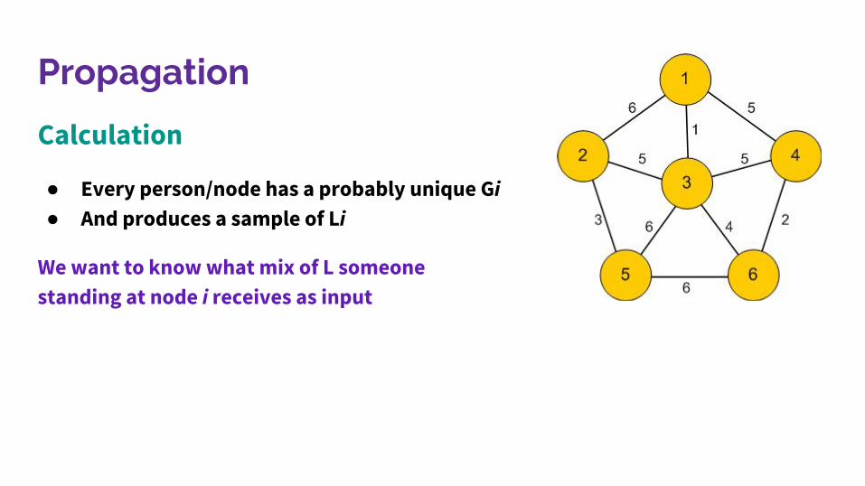
● Every person/node has a probably unique Gi● And produces a sample of Li
Propagation
Calculation
● Every person/node has a probably unique Gi● And produces a sample of Li
We want to know what mix of L someone standing at node i receives as input

Propagation
Calculation
● Every person/node has a probably unique Gi● And produces a sample of Li
We want to know what mix of L someone standing at node i receives as input
Simplifying the calculation,Someone at node 1 hears 6-parts L2, 1-part L3, and 5-parts L4

Acquisition
● How does each learner react to her unique mix of L?
Acquisition
● How does each learner react to her unique mix of L?● Dependent on the learning model

Acquisition
● How does each learner react to her unique mix of L?● Dependent on the learning model● Many learning models can be slotted in
○ trigger-based learner (Gibson & Wexler 1994)○ Variational learner (Yang 2000)○ Anything that operates on probabilities...

Population Size and Grammars

Background
● Simulations typically run with a few hundred agents ○ Kauhanen 2016, Stanford & Kenny 2013, Blythe & Croft 2012, etc.
● Is this true of actual speech communities?

Background
● Simulations typically run with a few hundred agents ○ Kauhanen 2016, Stanford & Kenny 2013, Blythe & Croft 2012, etc.
● Is this true of actual speech communities?○ Maybe sometimes!

Background
● Simulations typically run with a few hundred agents ○ Kauhanen 2016, Stanford & Kenny 2013, Blythe & Croft 2012, etc.
● Is this true of actual speech communities?○ Maybe sometimes!○ But not typically true of the communities under study
● Martha’s Vineyard (Labov 1963)○ ~5,500 in winter → ~42,000 in summer c. 1960○ Summer population largely from New England (cf Massachusetts 5.1mil in 1960)
Background
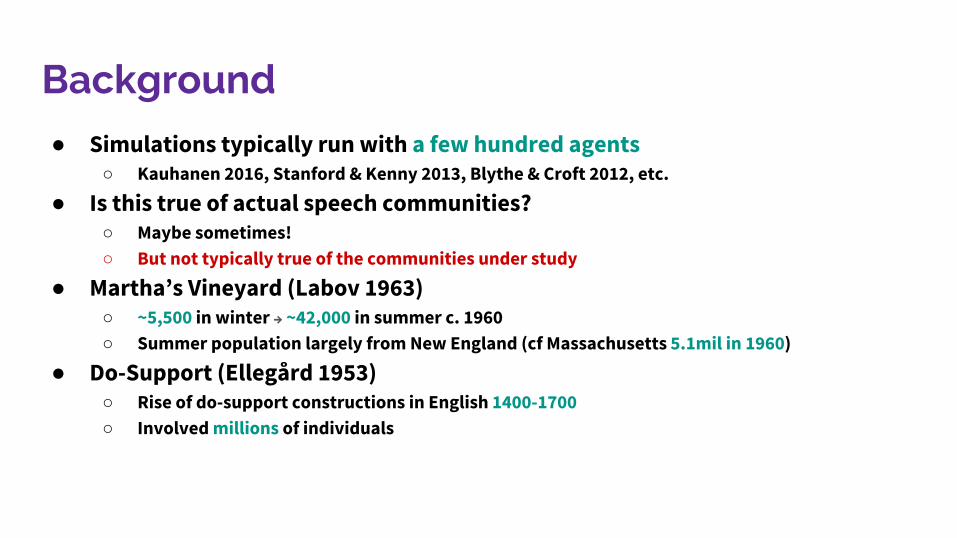
● Simulations typically run with a few hundred agents○ Kauhanen 2016, Stanford & Kenny 2013, Blythe & Croft 2012, etc.
● Is this true of actual speech communities?○ Maybe sometimes!○ But not typically true of the communities under study
● Martha’s Vineyard (Labov 1963)○ ~5,500 in winter → ~42,000 in summer c. 1960○ Summer population largely from New England (cf Massachusetts 5.1mil in 1960)
● Do-Support (Ellegård 1953)○ Rise of do-support constructions in English 1400-1700○ Involved millions of individuals

When is this a Problem?
● If learners internalize a distribution of grammars (e.g. competing grammars) and the population is (approximately) uniformly mixed, it is not a problem
○ Change closely approximates the path followed in infinite populations○ So small-population models are a useful convenience
● But, if either of the above does not hold, it is a problem (maybe)○ It becomes impossible to untangle population and learning effects

Demonstration: Neutral Change
● Assume two connected communities○ C1 begins with 100% Grammar 1○ C2 begins with 100% Grammar 2

Demonstration: Neutral Change
● Assume two connected communities○ C1 begins with 100% Grammar 1○ C2 begins with 100% Grammar 2
● Neutral change

Demonstration: Neutral Change
● Assume two connected communities○ C1 begins with 100% Grammar 1○ C2 begins with 100% Grammar 2
● Neutral change● Over time, each community should
approach 50/50 mix

Demonstration: Neutral Change
● Assume two connected communities○ C1 begins with 100% Grammar 1○ C2 begins with 100% Grammar 2
● Neutral change● Over time, each community should
approach 50/50 mix● Assume speakers internalize a single grammar
○ Chosen probabilistically from mix of L○ weighted by frequency in their input

Demonstration: Neutral Change
● Assume two connected communities○ C1 begins with 100% Grammar 1○ C2 begins with 100% Grammar 2
● Neutral change● Over time, each community should
approach 50/50 mix● Assume speakers internalize a single grammar
○ Chosen probabilistically from mix of L○ weighted by frequency in their input○ cf Kauhanen 2016
Rise of G2 in C1n = 200
Red curve predictedBlue curves first 10 trials

n = 200 n = 2,000 n = 20,000

n = 200 n = 2,000 n = 20,000
Most trials fix at 0% or 100%
Most trials hover near50%

Demonstration: Advantage
● Repeating the previous test but with an advantage○ Single community beginning at 1% innovative grammar○ Learners choose a single grammar probabilistically, weighted toward innovative○ Logistic curve predicted
n = 200 n = 2,000 n = 20,000

Demonstration: Advantage
● At small n, S-curve change cannot arise
n = 200 n = 2,000 n = 20,000
Looks a lot like neutral change did!

Demonstration: Advantage
● At small n, S-curve change cannot arise● At large n, S-curves become smooth
n = 200 n = 2,000 n = 20,000
Looks a lot like neutral change did!

Conclusions
● “Innocuous” assumptions may dominate behavior○ Here, choice of population size and single-grammar assumptions○ Conclusions drawable for n=200 do not scale to n=20,000 or visa-versa
● Slightly different assumptions yield drastically different conclusions○ Is neutral change well-behaved? ○ Do we expect to see S-curve change?
● Most innovation is meaningless○ If innovation occurs in a corner of some (small) sub-community, it will probably die off fast

Complex Networks and S-Curves:The Cot-Caught Merger in New England

Single-Grammar Learners
● The previous section pointed out a problem with single-grammar learners● But it is not an indictment

Single-Grammar Learners
● The previous section pointed out a problem with single-grammar learners● But it is not an indictment● Some changes are neatly modeled as single-grammar processes
○ Can represent the loss of distinctions in the grammar○ E.g., the spread of mergers, e.g., cot-caught on the RI/MA border (Johnson 2007)

Modeling the loss of Distinction
● Claim: Mergers tend to spread because the merged grammar has a processing advantage

Modeling the loss of Distinction
● Claim: Mergers tend to spread because the merged grammar has a processing advantage
● When two speakers with the distinction (D+) talk, no misunderstanding
Modeling the loss of Distinction
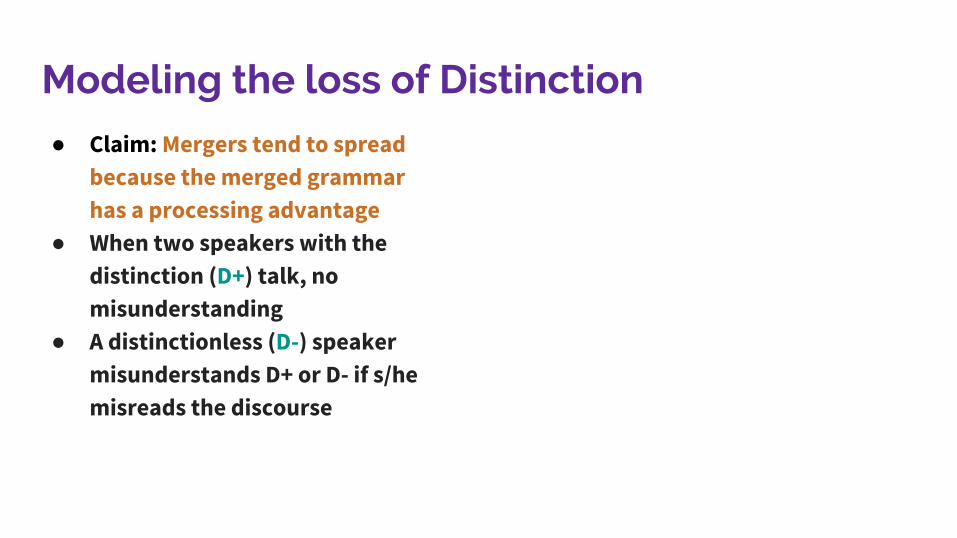
● Claim: Mergers tend to spread because the merged grammar has a processing advantage
● When two speakers with the distinction (D+) talk, no misunderstanding
● A distinctionless (D-) speaker misunderstands D+ or D- if s/he misreads the discourse

Modeling the loss of Distinction
● Claim: Mergers tend to spread because the merged grammar has a processing advantage
● When two speakers with the distinction (D+) talk, no misunderstanding
● A distinctionless (D-) speaker misunderstands D+ or D- if s/he misreads the discourse
● When D+ hears D-, D+ misunderstands when D- uses variant A but means B
● Is it better to be D+ or D-?● Depends on how many D- are
around

Modeling the loss of Distinction
● Claim: Mergers tend to spread because the merged grammar has a processing advantage
● When two speakers with the distinction (D+) talk, no misunderstanding
● A distinctionless (D-) speaker misunderstands D+ or D- if s/he misreads the discourse
● When D+ hears D-, D+ misunderstands when D- uses variant A but means B
● Is it better to be D+ or D-?● Depends on how many D- are
around● For a cot-caught variational
learner, D- is better if at least 17% of the input is D-

The Problem
● A variational learner in a near-uniform population fixes at 0% or 100% immediately
● Because the % of distinctionless speakers ≈ % distinctionless input● If < 17% are distinctionless, nobody will learn it● If > 17% are distinctionless, everybody will learn it● Not what has happened empirically

The Solution
● A more realistic network!

The Solution
● A more realistic network!● Large populations are not
homogeneous○ Tend to consist of many tight
clusters loosely connected together○ Echos of Milroy & Milroy’s “strong
and weak connections”

The Solution
● A more realistic network!● Large populations are not
homogeneous○ Tend to consist of many tight
clusters loosely connected together○ Echos of Milroy & Milroy’s “strong
and weak connections”○ Homophily○ Physical geography○ etc.

The Solution
● A more realistic network!● Large populations are not
homogeneous○ Tend to consist of many tight
clusters loosely connected together○ Echos of Milroy & Milroy’s “strong
and weak connections”○ Homophily○ Physical geography○ etc.
● So we consider a loosely connected network of centralized clusters

The Solution
● A network of 39 loosely connected centralized clusters - all unmerged
● Plus one merged cluster

The Solution
● A network of 39 loosely connected centralized clusters - all unmerged
● Plus one merged cluster● Clusters merges rapidly in
successionClusters

The Solution
● A network of 39 loosely connected centralized clusters - all unmerged
● Plus one merged cluster● Clusters merges rapidly in
succession● But the community average is an
S-curveClustersAverage

Properties of Change
The averaged S-curve slope: ● depends on the grammatical
advantage and the network
Trials

Properties of Change
The averaged S-curve slope ● depends on the grammatical
advantage and the network● is improved by evolving the
network
ClustersAverage

Properties of Change
The averaged S-curve slope ● depends on the grammatical
advantage and the network● is improved by evolving the
network● is preserved when introduced
with a time offset4 0 Offset
10 Offset20 Offset

Properties of Change
The averaged S-curve slope ● depends on the grammatical
advantage and the network● is improved by evolving the
network● is preserved when introduced
with a time offset○ Is compatible with the
Constant Rate Effect
4 0 Offset10 Offset20 Offset

Conclusions
Population models and learning models interact

Conclusions
Population models and learning models interact
● They conspire to yield empirical rates of change

Conclusions
Population models and learning models interact
● They conspire to yield empirical rates of change○ Higher slope indicates greater grammar/social advantage -or- more cohesive network○ Not possible to draw conclusions about a change’s advantage by slope alone

Conclusions
Population models and learning models interact
● They conspire to yield empirical rates of change● S-curve change is possible outside competing grammars scenarios
○ Even in small populations○ Therefore gradual change alone cannot be evidence for competing grammars
Conclusions
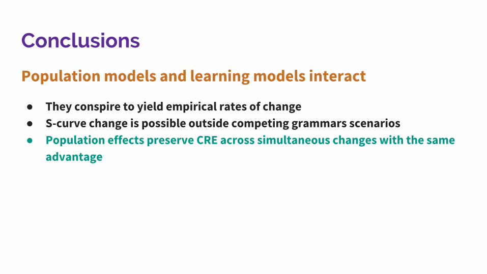
Population models and learning models interact
● They conspire to yield empirical rates of change● S-curve change is possible outside competing grammars scenarios● Population effects preserve CRE across simultaneous changes with the same
advantage

Conclusions
Population models and learning models interact
● They conspire to yield empirical rates of change● S-curve change is possible outside competing grammars scenarios● Population effects preserve CRE across simultaneous changes with the same
advantage● We have a solution looking for a problem

Questions?Code Available Here:
github.com/jkodner05/NetworksAndLangChange
Slides Available Here:
ling.upenn.edu/~jkodner

Extra slides: Maths

Diffusion
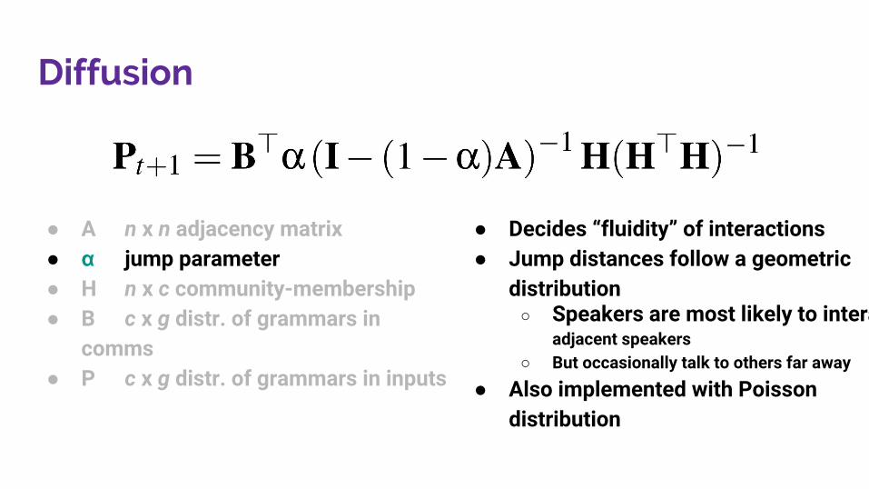
● A n x n adjacency matrix● α jump parameter● H n x c community-membership● B c x g distr. of grammars in comms● P c x g distr. of grammars in inputs

Diffusion
● A n x n adjacency matrix● α jump parameter● H n x c community-membership● B c x g distr. of grammars in
comms● P c x g distr. of grammars in inputs
The network graph
Who speaks what in what proportionWho hears what in what proportion

Diffusion
● A n x n adjacency matrix● α jump parameter● H n x c community-membership● B c x g distr. of grammars in
comms● P c x g distr. of grammars in inputs
● Indicates directed weighted edges between speakers in network
● Column stochastic● Easy to make undirected or
unweighted
Diffusion
● A n x n adjacency matrix● α jump parameter● H n x c community-membership● B c x g distr. of grammars in
comms● P c x g distr. of grammars in inputs
● Decides “fluidity” of interactions● Jump distances follow a geometric
distribution○ Speakers are most likely to interact with
adjacent speakers○ But occasionally talk to others far away
● Also implemented with Poisson distribution

Diffusion
● A n x n adjacency matrix● α jump parameter● H n x c community-membership● B c x g distr. of grammars in
comms● P c x g distr. of grammars in inputs
● Indicator matrix● Defines “community” membership● More on this later...

Diffusion
● A n x n adjacency matrix● α jump parameter● H n x c community-membership● B c x g distr. of grammars in
comms● P c x g distr. of grammars in inputs
● Distribution of grammars● According to which community
members produce utterances

Diffusion
● A n x n adjacency matrix● α jump parameter● H n x c community-membership● B c x g distr. of grammars in
comms● P c x g distr. of grammars in inputs
● Distribution of grammars● Heard by learners of each
community
Tracking Individuals
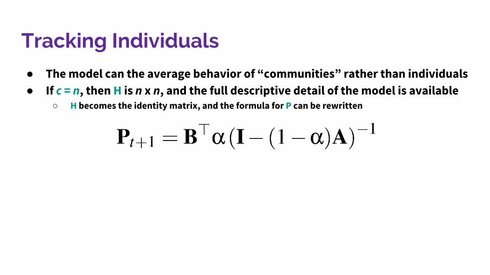
● The model can the average behavior of “communities” rather than individuals● If c = n, then H is n x n, and the full descriptive detail of the model is available
○ H becomes the identity matrix, and the formula for P can be rewritten

Tracking Communities
● If fine-grain detail is unnecessary, tracking community averages provides substantial computational speedup when c << n
● If each community is internally uniform, n x n A admits a c x c equitable-partition Aπ
● Yielding a more efficient but equivalent update formula for P
Anecdotally, I can run n = 20,000 nets on my laptop with Aπ about as fast as n = 2,000 net with A

Transmission
● Dependent on the learning model● Our implementation is modular, so many learning models can be slotted in
○ e.g., trigger-based learner (Gibson & Wexler 1994)○ Variational learner (Yang 2000)

Transmission
● Dependent on the learning model● Our implementation is modular, so many learning models can be slotted in
○ e.g., trigger-based learner (Gibson & Wexler 1994)○ Variational learner (Yang 2000)
● Let L be the distribution of grammars internalized by a learner who heard P○ L is a matrix consisting of g vectors l1, l2, … lg
● Define g transition matrices T1, T2, … Tg, one for each potential target grammar

Transmission and Grammatical Advantage
● If L = P, learners internalize variants at the rate they hear them○ This yields neutral change
● Otherwise, learners choose variants in a way that biases some over others○ Some variants have an advantage over others○ This yields S-curve change in perfectly mixed populations

Transmission Example
● Let there be two languages L1 and L2, the extensions of g1 and g2, produced with probabilities P1 and P2.
● a = P1[L1 union L2] 1 - a = P1[L1\L2]● b = P2[L1 union L2] 1 - b = P2[L2\L1]

Transmission Example
● Let there be two languages L1 and L2, the extensions of g1 and g2, produced with probabilities P1 and P2.
● a = P1[L1 union L2] 1 - a = P1[L1\L2]● b = P2[L1 union L2] 1 - b = P2[L2\L1]● Let T1 and T2 be transition matrices assuming g1 and g2 are the target
grammars respectively● T1 = [1 0 ; 1-a a] T2 = [b 1-b ; 0 1]

Transmission Example
T1 =�1 0� �1-a a�
T2 =�b 1-b� �0 1�
● If the target grammar is g1, then in the limit...

Transmission Example
T1 =�1 0� �1-a a�
T2 =�b 1-b� �0 1�
● If the target grammar is g1, then in the limit...
○ Learners who initially hypothesize g1 will always remain in g1

Transmission Example
T1 =�1 0� �1-a a�
T2 =�b 1-b� �0 1�
● If the target grammar is g1, then in the limit...
○ Learners who initially hypothesize g1 will always remain in g1
○ Learners who initially hypothesize g2 will remain at g2 with probability a

Transmission Example
T1 =�1 0� �1-a a�
T2 =�b 1-b� �0 1�
● If the target grammar is g1, then in the limit...
○ Learners who initially hypothesize g1 will always remain in g1
○ Learners who initially hypothesize g2 will remain at g2 with probability a
○ Or switch to g1 with probability 1-a

Extra Slides: NCS in the St. Louis Corridor
Not all Change is Ideal
● An empirical fact● Some change does not reach completion● So it is obviously not S-shaped
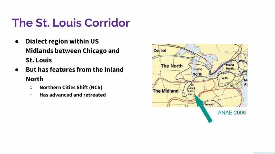
● Dialect region within US Midlands between Chicago and St. Louis
● But has features from the Inland North
○ Northern Cities Shift (NCS)○ Has advanced and retreated
ANAE 2006
The St. Louis Corridor

● NCS entered the Corridor via Route 66 during the Great Depression
Friedman 2014
The St. Louis Corridor

● NCS entered the Corridor via Route 66 during the Great Depression
● Path of change is different On-Route and Off-Route
○ NCS peaks first On-Route○ NCS peaks higher On-Route
Friedman 2014
The St. Louis Corridor

● NCS entered the Corridor via Route 66 during the Great Depression
● Path of change is different On-Route and Off-Route
○ NCS peaks first On-Route○ NCS peaks higher On-Route
Friedman 2014
The St. Louis CorridorOn-Route Off-Route

● NCS entered the Corridor via Route 66 during the Great Depression
● Path of change is different On-Route and Off-Route
○ NCS peaks first On-Route○ NCS peaks higher On-Route
● Typical of two-compartment systems
Wikipedia
The St. Louis Corridor
“On-Route”“Off-Route”

Modelling the Corridor: Network Structure
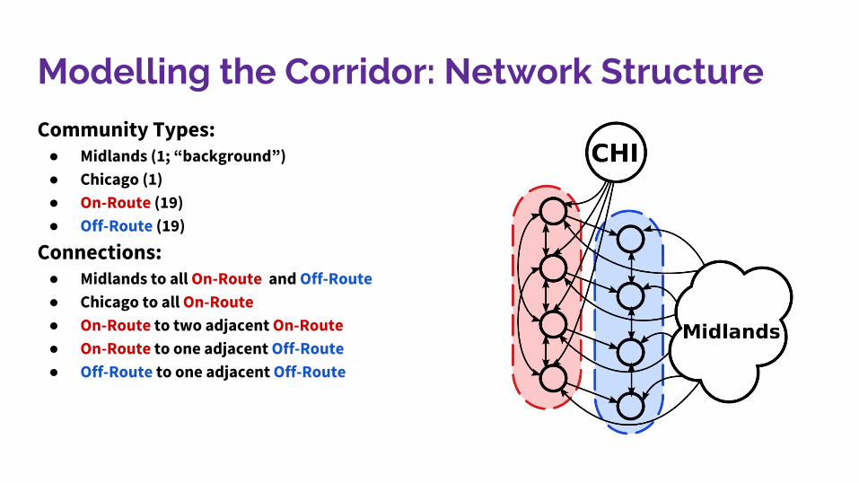
Community Types:● Midlands (1; “background”)● Chicago (1)● On-Route (19)● Off-Route (19)
Modelling the Corridor: Network Structure
Community Types:● Midlands (1; “background”)● Chicago (1)● On-Route (19)● Off-Route (19)
Connections:● Midlands to all On-Route and Off-Route● Chicago to all On-Route● On-Route to two adjacent On-Route● On-Route to one adjacent Off-Route● Off-Route to one adjacent Off-Route
7

Modelling the Corridor: History
● Vary a single parameter: Direction of movement to On-Route communities

Modelling the Corridor: History
● Vary a single parameter: Direction of movement to On-Route communities● Tests Great Depression hypothesis

Modelling the Corridor: History
● Vary a single parameter: Direction of movement to On-Route communities● Tests Great Depression hypothesis● It would be too “easy” if we could vary multiple parameters
○ Movement Off-Route○ Strength of connections between On-Route and Off-Route○ Strength of connections between On/Off-Route and Chicago/Midlands○ Advantage of NCS○ Etc.
● And the results would be less meaningful
Modelling the Corridor: History
● Vary a single parameter: Direction of movement to On-Route communities● Tests Great Depression hypothesis
Stage 1 - 5 iterationsNo movement (speaker interaction only)
Stage 2 - 20 iterations2% movement from Chicago to On-Route “Great Depression”
Stage 3 - 75 iterations2% movement from Midlands to On-Route “Post-Depression”

Modelling the Corridor: The Variable
● Treating the NCS as a single binary variable subject to competing grammars

Modelling the Corridor: The Variable
● Treating the NCS as a single binary variable subject to competing grammars● Community Variable Distributions:
○ Chicago fixed at 100% NCS+○ Midlands fixed at 100% NCS-○ On/Off-Route begins 100% NCS- but is allowed to vary

Modelling the Corridor: The Variable
● Treating the NCS as a single binary variable subject to competing grammars● Community Variable Distributions:
○ Chicago fixed at 100% NCS+○ Midlands fixed at 100% NCS-○ On/Off-Route begins 100% NCS- but is allowed to vary
● Tested as neutral, slightly advantaged, and heavily advantaged change

Results: Neutral Change
● A classic two-compartment pattern arises
- - - - End DepressionOn-Route Avg
On-Route Comms.Off-Route Avg
Off-Route Comms.

Results: Neutral Change
● A classic two-compartment pattern arises
● NCS peaks higher and earlier On-Route than Off-Route
- - - - End DepressionOn-Route Avg
On-Route Comms.Off-Route Avg
Off-Route Comms.

Results: Neutral Change
● A classic two-compartment pattern arises
● NCS peaks higher and earlier On-Route than Off-Route
● NCS continues to increase Off-Route even after On-Route population movements are reversed
- - - - End DepressionOn-Route Avg
On-Route Comms.Off-Route Avg
Off-Route Comms.

● Advantaged change resists being “tamped down” Off-Route
○ NCS recedes given a slight advantage○ NCS advances given a heavy
advantage
Results: Advantaged ChangeSlight Advantage
a=0.80, b=0.82
Heavy Advantagea=0.80, b=0.85

● Advantaged change resists being “tamped down” Off-Route
○ NCS recedes given a slight advantage○ NCS advances given a heavy
advantage
● Exists some threshold above which indirect action On-Route is insufficient
● Can be solved with additional model parameters
○ Rate of movement Off-Route○ The advantage itself○ etc.
Results: Advantaged ChangeSlight Advantage
a=0.80, b=0.82
Heavy Advantagea=0.80, b=0.85

Final Takeaways
Population models and learning models interact!

Final Takeaways
Population models and learning models interact!
● Assumptions must be carefully considered when modelling change○ Under what assumptions are results generalizable?

Final Takeaways
Population models and learning models interact!
● Assumptions must be carefully considered when modelling change○ Under what assumptions are results generalizable?
● Attested paths of change are governed by these interactions○ Sometimes explicitly e.g., the St. Louis Corridor○ Sometimes implicitly e.g., New England cot-caught