Embed Size (px)
Citation preview

DI
SC
US
SI
ON
P
AP
ER
S
ER
IE
S
Forschungsinstitut zur Zukunft der ArbeitInstitute for the Study of Labor
Population Policies, Demographic Structural Changes, and the Chinese Household Saving Puzzle
IZA DP No. 7026
November 2012
Suqin GeDennis Tao YangJunsen Zhang

Population Policies, Demographic Structural Changes, and the
Chinese Household Saving Puzzle
Suqin Ge Virginia Tech
Dennis Tao Yang
University of Virginia and IZA
Junsen Zhang
Chinese University of Hong Kong and IZA
Discussion Paper No. 7026 November 2012
IZA
P.O. Box 7240 53072 Bonn
Germany
Phone: +49-228-3894-0 Fax: +49-228-3894-180
E-mail: [email protected]
Any opinions expressed here are those of the author(s) and not those of IZA. Research published in this series may include views on policy, but the institute itself takes no institutional policy positions. The IZA research network is committed to the IZA Guiding Principles of Research Integrity. The Institute for the Study of Labor (IZA) in Bonn is a local and virtual international research center and a place of communication between science, politics and business. IZA is an independent nonprofit organization supported by Deutsche Post Foundation. The center is associated with the University of Bonn and offers a stimulating research environment through its international network, workshops and conferences, data service, project support, research visits and doctoral program. IZA engages in (i) original and internationally competitive research in all fields of labor economics, (ii) development of policy concepts, and (iii) dissemination of research results and concepts to the interested public. IZA Discussion Papers often represent preliminary work and are circulated to encourage discussion. Citation of such a paper should account for its provisional character. A revised version may be available directly from the author.

IZA Discussion Paper No. 7026 November 2012
ABSTRACT
Population Policies, Demographic Structural Changes, and the Chinese Household Saving Puzzle*
Using combined data from population censuses and Urban Household Surveys, we study the effects of demographic structural changes on the rise in household saving in China. Variations in fines across provinces on unauthorized births under the one-child policy and in cohort-specific fertility influenced by the implementation of population control policies are exploited to facilitate identification. We find evidence that older households with a reduced number of adult children save more because of old-age security concerns, middle-aged households experience an increase in saving due to the lighter burden of dependent children, and younger households save more because of having fewer siblings to share the responsibility of parental care. These findings lend support to a simple economic model in which the effects of population control policies are investigated in the context of household saving decisions in China. JEL Classification: E21, J11, J13 Keywords: household saving, one-child policy, demographic structure, cohort analysis,
China Corresponding author: Dennis Tao Yang Darden School of Business University of Virginia Charlottesville, VA 22903 USA E-mail: [email protected]
* Dennis Tao Yang would like to thank Jessie Pang for excellent research assistance. The financial support from the Research Grants Council of the Hong Kong Special Administrative Region, China (Project Number 457911) and the research support from the Hong Kong Institute of Asia-Pacific Studies are gratefully acknowledged.
1 Introduction
Household saving rate has increased dramatically over the past two decades in China, rising
from 16.1% in 1990 to 21.5% in 2005 (see Table 1). Behind the rise in average saving rate, the
age-saving profile has also evolved into an unusual pattern. In the early 1990s, saving rate
was relatively low for young families, and it increased with the age of household heads until
they were close to retirement. In recent years, however, household age-saving profiles have
turned into a U-shaped pattern, with younger and older households having relatively higher
saving rates (see Figure 1A). A more pronounced U-shaped increase in age-specific saving
rates is observed from 1990 to 2005 (see Figure 1B), as younger and older households raised
their saving rates by over 10 percentage points, much more than middle-aged households.1
According to the life cycle theory, young workers save little as they anticipate a rise in future
income; the saving rates of middle-aged workers are the highest when their earnings reach
the peak; and, saving rates become flat or even decline as workers approach retirement. Such
a “hump-shaped” life cycle pattern is often observed in typical cross-sectional analyses in
other economies (e.g., Attanasio, 1998; Jappelli and Modigliani, 2005). Recent studies to
explain the puzzling U-shaped age-saving profiles in China have focused on factors such as
the rising private burden of expenditures on housing, education, and health care (Chamon
and Prasad, 2010) and the changes in life cycle earnings profiles and incomplete pension
reforms in China (Song and Yang, 2010).
In this paper, we develop and test a new hypothesis that the demographic structural
changes resulting from a series of population control policies since the 1970s have contributed
to the changes in China’s household saving patterns.2 After population control policies came
into effect, birth rates for successive cohorts plummeted. Consequently, the demographic
1These findings are based on China’s Urban Household Surveys (UHS), which are described in detail inthe data section. See Chamon and Prasad (2010), Song and Yang (2010), and Yang, Zhang and Zhou (2012)for systematic documentation of age-specific household saving patterns in urban China.
2The demographic transition would also affect other aspects of the economy. See Song et al. (2012) for arecent study on the inter-relationship between China’s demographic transition and its economic growth andpension reforms.
1

structure shifted to a new regime in recent years in which young households have fewer
siblings, middle-aged households have fewer dependent children, and old households have
fewer adult children. Traditionally, the younger generation is supposed to provide old-age
support to their elderly parents in Chinese households. Having fewer siblings, the young
households will save more because of the increasing burden of providing upstream transfer
to their parents. Households with dependent children can save more with the lighter burden
of child care and education expenses. Older people have more incentive to save for old-age
security as a substitute for the reduced number of children.
We develop a simple overlapping generation (OLG) model to illustrate how population
control policies and demographic structural changes affect saving decisions of individuals at
different life stages. Incorporated into the model are key features of the Chinese household
structure: parents raise their dependent children; in turn, adult children provide monetary
transfers to their elderly parents as old-age support. The model allows parents to be altruistic
(treating children as consumption goods) and to use children for old-age support (treating
children as investment goods). Population control policies differentially affect the numbers
of siblings, dependent children, and adult children for households at different ages (i.e., from
different birth cohorts). The model predicts three testable hypotheses following binding
birth quota. First, the responsibility of parental care increases for adult children with fewer
siblings and their saving rate will increase. Second, households with fewer dependent children
will increase their saving because of less mouths to feed. Third, the smaller number of adult
children reduces old-age support for parents, thus encouraging the old to save more. These
predictions demonstrate how saving decisions of different cohorts respond to demographic
structural changes. The behavioral model provides guidance for estimating the relative
contributions of various factors behind the changes in age-saving profile in China.
We test the model implications and estimate the effects of demographic structural changes
on Chinese household saving using combined data from the Urban Household Surveys (UHS)
and population censuses. The UHS contains information on consumption expenditure at
2

the household level, but lacks detailed information on fertility histories. Thus, we match
the 1989—1991 and the 2004—2006 UHS with the 1990 and 2005 population censuses for
each single year-of-birth cohort in each province. The demographic structure experienced
dramatic changes from 1990 to 2005 as a consequence of the population control policies and
other socioeconomic changes since the early 1970s. For example, compared to their 1990
counterparts, young households headed by those between 26 and 35 years old had 1.9 fewer
siblings, middle-aged households headed by individuals in their 40s had 0.3 fewer dependent
children, and old households led by those in their 50s had 1.8 fewer adult children in 2005.
The main empirical challenge in estimating the effects of demographic structural changes
on saving is the endogenous nature of fertility decisions. Our identification relies on exoge-
nous variations in cohort-specific fertility generated by the different timing of population
control policies that affected different birth cohorts and by the interaction of birth cohorts
with fines across provinces on unauthorized births under the one-child policy. Effective imple-
mentation of China’s population control policies started in the early 1970s. The government
tightened population control over time, and eventually the one-child policy was implemented
in 1979. Given the timing of the population control policies, cohorts at childbearing ages
face downward pressure in fertility, while leaving fertility decisions largely unaffected for
previous cohorts. The varying intensity of the policies over time also implies that their im-
pact on fertility differs for successive cohorts affected by the policies. Under the one-child
policy, each family is allowed only one child in urban China, and fines are levied on second
or higher-parity births. A unique feature of the policy is that the means of implementa-
tion and vigor of enforcement of the policy differ across provinces. In particular, the fines
on excess birth vary greatly by province and year (Scharping, 2003; Ebenstein, 2010). We
exploit the exogenous variability in fertility difference between provinces with different fines
for successive cohorts that were exposed to population control policies of varying intensities
to facilitate identification. Specifically, we use the interactions of provincial fertility fines
with five-year cohort dummies as instruments for the number of children when estimating
3
the effects of demographic structural changes on savings. The important observation under-
lying the identification strategy is that fertility fines may have differential effects on fertility
decisions of different birth cohorts with varying fertility history at any given point of time.
Note that this identification strategy does not require fertility fines to be exogenous.
Using cohort-level cross-sectional data for 1990 and 2005, we find systematic evidence that
demographic structural changes have significant and sizable effects on saving rates. Younger
households between 26 and 40 years old increase saving rates by 2.6 to 4.3 percentage points
with response to one less sibling. Middle-aged households between 41 and 50 years old
save 12.1 to 29.2 percentage points more with one less dependent child. Older households
between 51 and 60 years old increase their saving rates by 1.9 to 4.6 percentage points if
they have one less adult child. These results confirm the three hypotheses derived from the
model. Simple “back-of-the-envelope”calculations based on our point estimates show that
the demographic structural changes as measured by variations in the number of siblings,
the number of dependent children, and the number of adult children can account for a large
portion of the changes in age-saving profile between 1990 and 2005. The rest of the changes
can be explained by other socioeconomic factors.
Although numerous studies have attempted to understand the rising household saving
in China in recent years, substantial uncertainty remains with regard to the driving forces.
Existing research emphasizes the importance of sharp cost increases in health and education
(Chamon and Prasad, 2010); competitive saving motive arising from the marriage market
(Wei and Zhang, 2011); structural shifts in life-cycle earnings (Song and Yang, 2010); and
the constraints of the household registration system (Chen, Lu and Zhong, 2012). Given
the dramatic changes in demographic structure, the existence of little empirical evidence on
its relationship with household age-saving profile is somewhat surprising. Several studies
attempt to investigate the link between demographic structure and household saving at
the aggregate level (Modigliani and Cao, 2004; Horioka and Wan, 2007; Curtis, Lugauer,
and Mark, 2011). Using household data, Banerjee, Meng, and Qian (2010) investigate the
4

effects of fertility and child gender on parents’ saving decisions. They use a sample of
households headed by individuals between 51 and 65 years old, and therefore only study the
saving behavior of old households. Instead, we show that fertility influences saving behavior
differently for households at various stages of their life cycle. Aside from previous studies,
we highlight how age-specific saving decisions respond to demographic structural changes,
and investigate the shift of the entire age-saving profile over time.
The rest of this paper is organized as follows. Section 2 briefly describes the evolution of
China’s population policies and their impact on demographic structure. Section 3 presents a
simple OLG model that links population control policy, demographic structural change, and
household saving. The model provides a framework to specify and interpret our empirical
results. Section 4 describes the data and variables. Section 5 discusses the empirical strategy
and presents the results on the effects of demographic changes on household saving rates by
age. Section 6 concludes.
2 Population Control Policies in China
China has witnessed major changes in its population policies over the past few decades,
moving from encouraging population growth to strictly enforcing population control. In the
early 1950s, Chinese families were encouraged to have children. The population rose from
550 million in 1950 to 830 million by 1970. The rapid population growth during the 1950s
and 1960s led to the “Wan (Later), Xi (Longer), Shao (Fewer)”campaign of the 1970s. This
policy called for later marriage and child bearing, wider spacing between births, and fewer
children. Education, propaganda, and persuasion were the offi cially stated means of policy
implementation (Yang and Chen, 2004). Men were encouraged to marry no earlier than 28
years old and women no earlier than 25 years old. Couples were persuaded to allow at least
a four-year gap after the first child before having another baby. Urban families were also
suggested to limit their number of children to two. The total fertility rate plummeted from
5
close to 6 in 1970 to less than 3 by the end of the 1970s (Coale, 1984).
However, population growth remained high; the baby boomers of the 1950s and 1960s
were entering their reproductive years, and by 1979, approximately two-thirds of the popu-
lation were under 30 years old. When economic reform was launched in the late 1970s, the
government considered curbing population growth as essential to economic expansion and to
an improvement in the standard of living. In 1979, the authorities tightened their population
control and introduced the one-child policy, which allows each household to have only one
child. Households were given birth quotas, and “above-quota”births were penalized. This
policy aimed to limit China’s population to 1.2 billion by 2000. After the implementation of
the one-child policy, the total fertility rate declined gradually from just below 3 in 1979 until
1995, and then more or less stabilized at approximately 1.7 (Hesketh, Lu and Zhu 2005).
Despite its name, the one-child rule does not equally apply to all Chinese families. Eth-
nic minorities are initially excluded from the policy.3 For urban residents and government
employees of Han ethnicity, the one-child policy is strictly enforced, with few exceptions. If
both parents are only children, they are allowed to have more than one child provided that
the birth spacing of children is more than four years. Families in which the first child has a
mental or physical disability or both parents work in high-risk occupations (i.e., mining) are
allowed to have another child.4
The State Family Planning Bureau sets the overall population control targets and policy
direction. However, the implementation of the policy varies from one locale to another.
Family-planning committees at the provincial and county levels devise local strategies for
implementing the state policy of population control, under the general principle of one child
per couple. Residents of different provinces are subject to different birth limits permitted
3China offi cially recognizes 56 distinct ethnic groups, with Han Chinese being the largest and comprisingapproximately 92% of the total population. See Li and Zhang (2009) for details on the one-child policyapplied to ethnic minorities.
4Our discussion of the population control policies has focused on urban areas as our empirical analysis isbased on an urban sample. Population control is generally less strict in rural areas. For example, in ruralareas, a second child is allowed after five years, but this provision sometimes applies only if the first childis a girl– in recognition of the traditional preference for boys and the reality in rural areas of the need formale labor.
6

by the local policy (Gu et al. 2007). Economic incentives are provided for compliance, and
noncompliance leads to substantial fines and possibly other nonfinancial penalties. Various
studies have shown that these fines are heavy and vary enormously across provinces. The fines
range from 20% to 200% of a household’s annual income (Short and Zhai 1998; Ebenstein
2010). Even at the lower end of the range, the fines are still substantial.
The rapid decrease in birth rate, combined with improving life expectancy, has led to
a significant change in the age structure of the Chinese population.5 The decline in child
dependency ratio (defined as the ratio between the children population aged 14 years or
below and the working-age population between 15 and 64 years, expressed in %) and rise
in old-age dependency ratio (defined as the ratio between the population aged 65 years or
above and the working-age population, expressed in %) are the major trends in China’s
demographic structure (Figure 2). We further plot the more detailed population structure
change (United Nations, 2008) in Figure 3. In 1970, the population structure was a pyramid
with a large base of young people. The number of children declined significantly over time
due to the sequence of population control policies. More relevant to this study, we observe
a clear regime shift of population age structure between 1990 and 2010. The proportion
of the population between 50 and 60 years old was 7% in 1990 and stood at 12% in 2010,
and these age cohorts experienced a rapid fertility decline as shown by the shrinking size
of young workers in their 20s and early 30s. The proportion of the middle-aged between
40 and 50 years old increased from 10% in 1990 to 16% in 2010, whereas their children’s
generation reduced in size. The proportion of the population below the age of 15 years was
28% in 1990 and dropped to 20% in 2010. In Chinese tradition, children are the source of
old-age support. The fertility decline induced by the population control policies has severely
curtailed this tradition.5Another outcome of family planning was an increase in the male-female ratio in China (Ebenstein 2010;
Li, Yi and Zhang, 2011).
7
3 A Simple Theoretical Framework
We postulate that China’s population control policies and demographic shifts have had a
profound impact on household saving behavior over the lifetime. One major diffi culty in
assessing these impacts is that, concurrently with the implementation of family planning
programs and the demographic transition since the early 1970s, fundamental socioeconomic
changes have occurred in China. The rising household saving took place against the backdrop
of China’s transition to a market economy and rapid income growth. Institutional reforms
have occurred whereby health care systems, education finance, pension arrangement, and
other social welfare provisions have evolved with the transition to a market economy. Other
elements, such as the rising household income, increasing overall macroeconomic uncertainty,
housing reform, and rising housing price, occurred during the same period, and likely have
affected household saving behavior.
In this section, we present a simple OLG model to focus on the effects of population
policies and demographic changes by holding other socioeconomic variables constant. The
model is useful in justifying the empirical specification we use and in interpreting the em-
pirical results. According to the model, changes in population control policies have different
effects on saving rates for individuals at different points in their lifetime. We will make these
relationships precise in the model and form our empirical specification based on them. In
the empirical analysis, we will also consider the effects of other socioeconomic variables aside
from the demographic shifts induced by population control policies.
3.1 The Model
The economy is populated with overlapping generations, referred to as the children, the
school-aged youth, the young, middle-aged and old workers, and the retired. We assume that
people start making economic decisions when they become young workers. In each of the
working-age periods, all workers supply one unit of labor inelastically. Let the socioeconomic
8

environment and the information set available be denoted by ψ. The after-tax earnings of
the young, middle-aged, and old workers are denoted by y1, y2, and y3, respectively. When
people retire, they receive the pension benefits of y4.
A generic individual has children when young. Each individual has a utility function,
u(c, f), and extracts positive utility from both consumption (c) and quantity of children
(f) . For simplicity, we do not consider the quality of children. Given the socioeconomic
environment, preferences for a young worker are represented by
4∑i=1
βi−1u (ci, f ;ψ) (1)
where β denotes the discount factor, and ci stands for consumption of an individual of age i
(i = 1, 2, 3 refers to the three working ages, respectively, and i = 4 refers to retirement). In
the empirical analysis, we will focus on the behaviors of working-age individuals between 26
and 60 years old. Almost all individuals have completed formal schooling by age 26, and by
age 60, all Chinese workers are offi cially retired.
The model allows parents to be altruistic, and they pay q to raise each child. The cost
of children incurs over time from a child’s birth to school age, until the child becomes a
working young adult. In the model, people have children when they are young adults; as the
children grow into school age, the parents are in their middle age. For illustration purpose,
we assume that the middle-aged parents pay the cost q for their school-aged children. The
child cost q includes household expenditure on children in terms of food, clothes, and shelter,
the opportunity cost in terms of parental time, and schooling expenses.
Following the Chinese tradition, parents also use children for old-age support. We assume
that there exists a targeted level of old-age support for parent, R, equally shared by all adult
children. Adult children are expected to take care of their elderly parents after retirement
as long as they are around. Given that early retirement starts at around age 50,6 we assume
6The offi cial retirement age is 50 for women in blue-collar jobs, 55 for other women, and 60 for men.Disabled workers may retire ten years earlier, and workers from bankrupt state-owned enterprises may retirefive years earlier.
9

that a young adult pays his/her share of parental support R/ns to the old parent, where ns
is the number of siblings (including oneself). If no uncertainty arises and every child pays
his/her share, an old parent receives a transfer of R from all the children. Figure 4 presents
the time line of inter-generational transfers.
Although almost all parents would pay to raise their dependent children, the old-age
support paid to elderly parents follows social norm and is rather voluntary. If some adult
children do not pay for their parents’old-age support because of mortality risk, financial
diffi culty, or in defiance of tradition, the likelihood to secure old-age support from adult
children would increase with the number of children. That is, the old-age support R becomes
an increasing function of the number of adult children, or R′ (f) > 0. Furthermore, we
assume that each adult child’s share of parental care, R(f)/f, decreases in the total number
of children.
Therefore, a young worker chooses the optimal saving decision by maximizing lifetime
utility subject to the following inter-temporal budget constraint:
c1 +R(ns)
ns+c2 + fq
1 + r+
4∑i=3
ci(1 + r)i−1
=4∑i=1
yi(1 + r)i−1
+R(f)
(1 + r)2, (2)
where r is the interest rate. The fertility variable f represents both the number of depen-
dent children for the middle-aged households and the number of adult children for the old
households.
Assuming log utility in consumption and separability in consumption and number of
children, the saving decision of the young solves
max
4∑i=1
βi−1 log ci (ψ) + λG[f (ψ)]
subject to the budget constraint (2). Children enter parents’utility through function G (·) ,
and the parameter λ measures the degree parents care about their children. The parameter
ψ represents the socioeconomic environment determined outside the model.
10

The Euler equation implies the following consumption pattern over the lifetime,
c1 (ψ) =c2 (ψ)
β(1 + r)=
c3 (ψ)
β2 (1 + r)2=
c4 (ψ)
β3(1 + r)3. (3)
If fertility is optimally chosen, then the optimal number of children f ∗, given ψ, satisfies
ρq(1 + r)−R′[f ∗ (ψ)]
λ(1 + r)2G′[f ∗ (ψ)]+f ∗ (ψ) q
1 + r=
4∑i=1
yi(1 + r)i−1
+ T (f ∗, ns),
where ρ = 1+β+β2+β3, and the term T (f ∗, ns) = R[f ∗ (ψ)]/(1+r)2−R (ns) /ns measures
each individual’s net gains through inter-generational transfers of old-age support. Positive
T implies net positive transfer from children, whereas negative T implies net transfer to
parents. Transfers from children increase in the number of adult children, and the burden
of parental support decreases in the number of siblings. Thus, the net gain T increases both
in the number of adult children and the number of siblings.
It is easy to show that saving rate when young equals
s1 (ψ) =y1 − c1y1
= 1− 1ρ×[
4∑i=1
yiy1(1 + r)i−1
− f ∗ (ψ) q
y1(1 + r)+T (f ∗, ns)
y1
]. (4)
For a young individual, the saving plan for the middle-aged and old periods are given by
s2 (ψ) =y2 − c2 − f ∗ (ψ) q
y2
= 1− β
ρ×[
4∑i=1
yiy2(1 + r)i−2
+(1 + β2 + β3)f ∗ (ψ) q
βy2+T (f ∗, ns)(1 + r)
y2
]; (5)
s3 (ψ) =y3 − c3y3
= 1− β2
ρ×[
4∑i=1
yiy3(1 + r)i−3
− (1 + r)f ∗ (ψ) q
y3+T (f ∗, ns)(1 + r)2
y3
]. (6)
In the initial equilibrium, no population control policy exists, and the socioeconomic envi-
ronment is fixed at ψ. Equations (4) to (6) present household saving rates over the life cycle.
11

If we further assume that all households face the same life-cycle earning profile, interest
rate and discount rate, then Equations (4) to (6) also illustrate the age-saving profile for a
cross-section of households at a steady state equilibrium.
In our empirical work, we look at a cross section of individuals at different life stages.
There are two ways to interpret the life cycle decision of Equations (4) to (6) of a given
individual in a cross-sectional context. The first way is to assume that different birth cohorts
have the same ψ (which does seem unrealistic). At a given point of time, Equations (4), (5),
and (6) would apply to the young, middle-aged, and old households, respectively. Thus, a
change in ψ will have different effects on individuals of different cohorts. The second way is to
assume that different birth cohorts have different ψ. Then, again, Equations (4), (5), and (6)
would correspond to the young, middle-aged, and old households, respectively. Any change
in ψ will have more different effects on individuals of different cohorts than under the first
interpretation. Either way, Equations (4) to (6) imply that population policies would have
different effects on individuals of different birth cohorts and that the resulting demographic
structural changes would also have different effects on individuals at different life stages at
a given point of time. The age-specific effects of demographic structural changes will be
further discussed in the next section.
3.2 Population Control Policies
In the context of household saving decisions in China in the past two decades, households
face many uncertainties against the backdrop of China’s transition to a market economy
and rapid income growth. For example, the socioeconomic environment and demographic
structure have both changed dramatically over time. These shocks will shift the saving profile
over time. We are particularly interested in the impact of demographic changes caused by
population control policy on saving rates.
Suppose the state population policy set the maximum number of children each couple
can have at f and f < f ∗. Given the binding birth quota, households make constrained
12
optimization by setting f = f. Initially, households that had passed childbearing age were
unaffected by the policy. For those influenced by the policy, the policy might come as a
surprise. For instance, a 26-year-old woman in 1977 did not anticipate the one-child policy
and made a lifetime saving decision based on her optimal fertility rate, say f ∗ = 2. At age
28, the one-child policy was implemented, such that each family has a birth quota of f = 1.
If the household had not reached its optimum of two children, it would reoptimize at age 28
given the accumulated asset at age 27. The marginal effects of fertility reduction on saving
generated by an unanticipated change in population policy are different from those generated
by the same but anticipated change in the policy.
Eventually, the economy will converge to a new steady state equilibrium in which all
individuals are exposed to the population control policy and fully anticipate the fertility
constraint. At this equilibrium, the consumption pattern of the households still follows
Equation (3). Optimal consumption over lifetime can be solved by combining the budget
constraint (2) and first-order conditions (3). The saving rates for households of different ages
are determined by Equations (4) to (6) by replacing f ∗ and ns with f, when lifetime earnings
and other socioeconomic variables are held constant. As Equations (4) to (6) show, changes
in the number of children or the number of siblings induced by the population policy have
different effects on the saving rates of individuals at different points of their lifetime.
It takes a few decades for all birth cohorts in an economy to be fully exposed to the
population control policy and reach constrained optimization. A more relevant analysis for
our purpose is to consider how households of different ages have responded to the implemen-
tation of the population control policies since the early 1970s. Specifically, we focus on three
age groups in 2005, and investigate how these three age cohorts’saving behavior changes
relative to the benchmark steady state equilibrium without family planning.
For the old households in 2005, their number of siblings is unaffected by the population
control policies. As the number of children (f) goes down, as shown in Equation (6), two
opposing effects on their saving exist. The first effect is the substitution between old-age
13

support from adult children and own saving. When people have fewer adult children, the
net transfer T goes down and precautionary saving is induced because of old-age security
concerns. The possibility that the precautionary motive induced by the reduced number
of adult children could interact with other uncertainty also arises. For example, if public
pension is reduced, people will rely more on private saving or children’s old-age support for
retirement. In this case, the reduced old-age support due to fewer adult children may induce
even more private savings. On the other hand, an indirect effect of the number of children
on the saving of old households emerges. These households had fewer dependent children
to support when they were younger. As expenditure on dependent children decreases, more
income is available for consumption over the lifetime. Therefore consumption expenditure
increases and people save less, as the second term in the bracket in Equation (6) shows.
Although the effect of fertility decline on old households’saving is theoretically ambiguous,
we postulate that the old-age security effect dominates, especially when the number of adult
children is considered. This assumption leads to the following hypothesis.
Hypothesis 1: As the number of adult children decreases, old households will save more for
the purpose of old-age security.
For the middle-aged households in 2005, their number of siblings is also unaffected by
the population policies. After the implementation of the population control policies, these
households have fewer dependent children and less mouths to feed. Thus, they can spend
less on children and save more, as shown by replacing f ∗ with f in the second term in the
bracket in Equation (5). The number of mouths to feed effect should apply to any household
with dependent children. This inference leads to the second hypothesis derived from the
model that can be tested empirically.
Hypothesis 2: As the number of children decreases, middle-aged households with dependent
children to support will increase their saving because of less mouths to feed.
Younger households in 2005 are not only subject to the birth quota, but their parents’
14

fertility decisions are also likely affected by the population control policies. Thus, they have
a smaller number of siblings compared to the birth cohorts in the benchmark steady state
equilibrium. In Equation (4), as ns declines, each person’s burden of parental care increases
and the net transfer from children T (f, ns) goes down. Therefore, individuals will consume
less and save more.
Hypothesis 3: As the number of siblings decreases, young households will save more to provide
old-age support to parents.
Concurrently with the implementations of population control programs, China has un-
dergone profound socioeconomic changes. The simple model presented in this section takes
all of them as given and focuses on the effects of population policies on household savings.
In the empirical analysis, we will try to make them explicit.
4 Data
Our empirical analysis aims to test the hypotheses postulated in the model and assess the ef-
fects of population control policies and demographic structural changes on household saving.
A data set suited to our purpose should contain the following information: first, accurate
measures of household saving rates for multiple years; second, cohort-specific data on family
composition, including complete information on the numbers of adult children, dependent
children, and siblings for successive cohorts; third, good measures of time or regional vari-
ations in population control policies; and fourth, other household demographic information
and socioeconomic variables that may affect saving decision. To fulfill the data requirement
on saving rates, we need repeated household income and expenditure surveys. Although
household surveys often have rich demographic information, they are typically residency-
based; thus, a household member is observed only if the person lives with the household
head. The majority of adult children and some dependent children in post-secondary school
do not live with parents, and adult siblings typically live in separate households. Therefore,
15
inferring the complete family composition information that fits our need at the household
level is not possible. The household sample alone is insuffi cient to test the model hypotheses.
Our strategy is to construct a cohort-based sample that meets all data requirements
using multiple data sources. The saving data we use come from the UHS conducted by
China’s National Bureau of Statistics (NBS). The UHS is an on-going income and expen-
diture survey of Chinese urban households, and it is known to be the best micro data on
household saving in China. The survey also records detailed information on employment,
wages, and demographic characteristics of all household members in each calendar year. The
second main data source is the Chinese population censuses. The censuses contain the most
comprehensive demographic information of Chinese households and provide information on
the family composition of different cohorts. We match them with the saving information of
the same cohorts from the UHS. We likewise collect province- and time-specific fine/income
ratio, which is the ratio between above-quota fertility fines and annual household income
under the one-child policy, as a measure for the strictness of the population control policy.
We also collect other socioeconomic variables that may affect household saving from various
sources. The strength of our cohort-based sample is that it not only combines the best
available household saving data with the most comprehensive demographic information, but
also contains policy variations that facilitate identification.
For the current analysis, we use UHS data from six provinces that are broadly repre-
sentative of China’s rich regional variation, namely, Beijing, Liaoning, Zhejiang, Sichuan,
Guangdong, and Shaanxi. Beijing is the rapidly growing capital city in the north; Guang-
dong and Zhejiang are dynamic high-growth provinces in the south coastal region; Liaoning
is a heavy-industry province in the northeast; and Sichuan and Shaanxi are relatively less
developed inland provinces located in the southwest and northwest, respectively. In the
UHS, each household reports data on expenditure on different commodities. We construct
a standard measure of household consumption that includes expenditure on goods and ser-
vices (including rent), interest payments on mortgages, vehicle loans and other loans, cash
16

contributions to organizations, and insurance premiums. We have also considered alterna-
tive consumption measures that exclude various items, which might be considered as saving.
Specifically, we first exclude expenditure on durables, then on health and education, which
can be considered as investment in human capital, and finally on mortgage payments. Income
is defined as total disposable family income, which includes earnings, transfers, capital in-
come, and pensions net of all income taxes and social security contributions. Saving is defined
as the difference between disposable income and consumption.7 Saving rates are computed
as the ratio of saving to income. Using alternative household consumption measures causes
no major changes to the facts documented below, except for saving rates after retirement.
Saving rates after retirement are not quantitatively important; hence, throughout the paper,
we shall focus on the saving behavior of working-age households with household head age
between 26 and 55 (for female) or 60 (for male).
We use UHS data to construct household age-saving profiles for 1990 and 2005. Given the
limited sample size, we combine the observations from the 1989—1991 surveys as representing
1990 and similarly, observations from 2004—2006 as representing 2005. An age-specific saving
rate is derived from averaging household saving rates for all households with the same age in
each period. Panel A of Figure 1 presents age-saving profiles for the two periods. Considering
that some age cells contain few observations, we use three-age moving average to minimize
the effect of measurement error. In the 1989—1991 period, the saving rates are relatively flat
before age 40 and then increase toward the retirement age. For the 2004—2006 period, age-
saving profile exhibits a dramatic change: it turns to a U-shape. Using alternative saving
definitions results in a qualitatively similar U-shaped profile. We further eliminate fixed
life-cycle effects by taking the difference of the two profiles. The outcome yields the increase
7The saving definition we adopt treats social security contribution as taxes, but this contribution can alsobe recognized as mandatory life-cycle saving (Jappelli and Modigliani, 2003). We are unable to construct aconsistent saving measure including social security contribution because no information is available for socialsecurity contribution in the 1989-1991 UHS. For the 2004-2006 period, households on average contribute5.2% to 8.4% of the household income to social security, with households between age 41 and 50 makingthe highest contribution. Therefore the 2004-2006 age-saving profile in Figure 1A would be higher and theU-shape slightly less pronounced if social security contribution is included.
17

in saving rates by age from 1989—1991 to 2004-2006, as depicted in panel B of Figure 1. The
U-shaped pattern becomes more pronounced: the average increase of saving rates for those
aged below 40 and above 50 is equal to 10.7 and 7.6 percentage points, respectively, whereas
that for those between 40 and 50 years old is only 3.5 percentage points. The rise in the
saving rates of the young and the old among working-age households sharply contrasts with
the typical hump-shaped or relatively flat age-saving profile.8
Each age cohort between 26 and 60 in 1990 and 2005 corresponds to a birth cohort
born between 1930 and 1979. These age cohorts have had different exposure under China’s
population policies over time. Among them, the older ones born in the 1930s had children in
the 1950s and 1960s when no population control policy was implemented; those born in the
1940s and early 1950s experienced the “Later, Longer, Fewer”family planning program in
the 1970s; those born in the late 1950s and onwards were all subject to the one-child policy
at their childbearing age; finally, the youngest cohort was likely born as the only child in
the family. To construct the cohort-specific family composition and demographic structure
variables, potentially affected by the population control policies, we match the 1989—1991
and 2004—2006 UHS households with the 1990 population census and the 2005 1% census.
We use the census urban samples in the corresponding six provinces to be consistent with
the households from the UHS. In the censuses, all women between age 15 and 64 report the
number of children ever born to them, and each person in a household can be identified.
We consider three demographic variables that are investigated in the model and affected
by population policies. First, we construct a variable on cohort-specific average number of
children ever born, for households of each age between 26 and 60 in 1990 and 2005 and in each
province. Saving data from UHS are collected based on the age of the household head, but
fertility information from census is for women. The number of children is therefore computed
as a weighted average using the gender and marital status distribution of household heads.9
8For subsamples classified by household head’s education and gender, they also feature a U-shaped levelin 2005, as well as a U-shaped increase of saving profile.
9In particular, consider all household heads at age a in year t, and let j denote household type, such thatj = 1 corresponds to single male, and j = 2, 3, 4 corresponds to married male, single female, and married
18
In the empirical analysis, we use this variable as a proxy for the number of adult children.
Second, we create a variable on the number of dependent children. Dependent children are
defined as children aged below 15 and those above age 15 but are still attending school.
We count the number of dependent children each household has and compute the average
conditional on the household head’s age. Finally, we investigate the number of siblings each
age cohort has. Although we have information on how many children people have from the
population censuses, information on the number of siblings is unavailable. We proxy the
number of siblings by locating their parents’birth cohort and collecting information on its
number of children.10
Panel A of Figure 5 presents the age-specific average number of children ever born from
the 1990 and 2005 censuses. In 1990, the young households between 26 and 35 years old
on average have one child. They were below age 24 in 1979 when the one-child policy was
first implemented, and therefore were constrained by the policy. Those over age 35 have
more children because the corresponding birth cohorts have had children or passed their
childbearing ages when the one-child policy was imposed. The increase in the number of
children by age reflects both the cumulative fertility effect over the life cycle and the declining
fertility rate over time since the mid-1960s, under various population control policies. In
2005, the age profile shows a dramatic change: the number of children hovers around one for
all households between 26 and 50 years old, and then it increases and reaches less than three
at the age of 60. This pattern is closely related to the population control policies. Those
aged between 26 and 50 in the 2005 census were all younger than 24 when the one-child
female, respectively. We first compute the proportions of households given the heads’gender and maritalstatus P ja,t. From the censuses, women of all ages report the number of children ever born, and thereforewe have fertility information for all female cohorts F ja,t with j = 3, 4. Now assume single men have nochildren. Men tend to marry younger women, and we identify the average age of women, a′, married tomen at age a in year t. The weighted fertility for age cohort a at time t in our sample is then computed asP 2a,tF
4a′,t + P
3a,tF
3a,t + P
4a,tF
4a,t.
10For example, those who were 40 years old in 2005 were born in 1965. Suppose on average their parentsgave birth at the age of 25, then their parents belong to the 1940 birth cohort. We use the average fertilityrates of 50-year-old individuals in 1990, who were born in 1940, as proxy for the number of siblings for the1965 birth cohort. We use the 1982, 1990, and 2005 censuses to construct the variable on the number ofsiblings.
19

policy was imposed, and therefore subject to the birth quota. We further eliminate fixed
life-cycle effects by taking the difference of the two profiles. The outcome yields the decline
in the number of children over age from 1990 to 2005, as depicted in panel B of Figure 5.
Households of all ages have fewer children in 2005, but the change is much more pronounced
for the older households. The average decline for those aged between 26 and 35 is 0.15
children. The decline increases in age, and by age 50, households in 2005 on average have
two fewer children compared to the 1990 households. If parents rely on adult children for
old-age support, the decrease in the number of children will have a larger effect on older
households.
In Figure 6, we present the changes in the number of dependent children from 1990 to
2005. Panel A shows that the age profile of dependent children is hump-shaped. The number
of dependent children increases with the age of household heads, reaches the peak at around
age 40, and then declines as children enter adulthood and leave the household. The age
profile of 2005 is lower than that of 1990 as fertility rate declines. As panel B of Figure 6
presents, for those between 26 and 40 years old, the 2005 households have on average 0.5
fewer dependent children compared to the 1990 households. Given that these households
have fewer dependent children to raise, they are likely to save more. For older households,
changes in the number of dependent children from 1990 to 2005 are much smaller.
Old-age support to the parents is typically shared among siblings. Therefore, one’s
responsibility for parental care depends on his/her number of siblings. Panel A of Figure
7 presents the age-specific average number of siblings (including oneself) in 1990 and 2005.
Even the very young households in 1990 were born in the 1960s, before the implementation
of population control policies. Young households between 26 and 35 years old had just
below four siblings, whereas older households had slightly more than four siblings. In 2005,
household heads belong to much younger birth cohorts, and were born between 1945 and
1979. Although the one-child policy had little effects on them, they experienced a dramatic
demographic transition in the 1970s due to the “Later, Longer, Fewer”campaign and other
20
socioeconomic changes. The average number of siblings increased from just above one to
more than four across age cohorts. Panel B of Figure 7 plots the changes in the number of
siblings by age from 1990 to 2005. Consistent with declining fertility rates, the number of
siblings decreased by around two for the very young households. The changes over time are
much smaller for older households, and for those aged 50 and above, the number of siblings
barely changes.
Combining household age-specific saving data from the UHS and the demographic infor-
mation of the corresponding birth cohorts from censuses, we have constructed a unique data
set based on age cohorts. We also explore the geographic variations in saving and demo-
graphic structural change. Average saving rates are computed for all households with the
same age between 26 and 60 years old in 1990 or 2005, located in one of the six provinces.
Accordingly, demographic variables including the number of children ever born, the number
of dependent children, and the number of siblings are constructed for the corresponding age
cohorts in each time period and province. We also consider other variables that may affect
household saving. For each age cohort in the sample, we construct variables on demographic
characteristics, such as the proportion of people having high school or above education, the
proportion of minorities, and the proportion of state employees. Following Wei and Zhang
(2011), we use the local sex ratio for age cohorts between 7 and 21 to measure the com-
petitiveness of the marriage market. The other province- and time-specific socioeconomic
variable we consider is the government spending on social security per person, taken from
the statistical yearbooks. Finally, under the one-child policy, the strictness of the policy
can be measured by province- and time-specific fine/income ratio for unauthorized births.
This aspect provides an important source of variation for the demographic structural change.
The fine/income ratio is the ratio between above-quota fertility fines and annual household
income, taken from Ebenstein (2010).
Summary statistics are presented in Table 1. The sample consists of 416 observations,11
11We have data for 35 age cohorts (between age 26 and 60) in two years and in six provinces(35× 2× 6 = 420). Four observations are missing because saving rates are not observed for the corresponding
21

with an average saving rate increasing from 16.07% to 21.47%. As a result of the population
control policies and demographic transition, the average number of children declined from
1.99 to 1.22 between 1990 and 2005, the average number of dependent children dropped
from 0.57 to 0.40, and the average number of siblings decreased from 4.01 to 3.17 during
the same time period. Between 1990 and 2005, the average working-age households became
much more educated, with high school completion rate increasing from 36.8% to 52.9%. The
proportion of minorities increased from 2.4% to 3.6%, and the share of state employment
dropped from 81.0% to 46.6%. The sex ratio increased from 104 in 1990 to 113 in 2005,
reflecting an increasing sex imbalance in China in recent decades. Government spending on
social security per person has also increased over time. Average fertility fines increased from
1.24 times of annual household income in 1990 to 3.25 times of annual household income in
2005.
5 Empirical Analysis
Our model provides useful guidance to formulate our empirical specifications, develop an
identification strategy, and help interpret our empirical findings. Although we mainly in-
vestigate the linkages between demographic changes and household saving, we will also in-
corporate other socioeconomic determinants of saving postulated in the literature into our
empirical framework.
5.1 Empirical Specifications
Based on the three hypotheses previously discussed, we model saving rates as a function of
the number of adult children, the number of dependent children, and the number of siblings to
capture the effects of demographic structure on savings. As we have shown in the behavioral
model, changes in demographic structure have different effects on households’saving rates
age, year, and province combinations.
22

at different points in their lifetime. Therefore, the effects of demographic variables on saving
are age-dependent. In the most flexible specification, we may allow these variables to have
interactions with all ages between 26 and 60 in the saving equation. This specification,
however, is hardly feasible given the small size of our cohort-based sample. Instead, we
define seven age-interval dummies (i = 1, 2, ..., 7) corresponding to ages between 26—30, 31—
35, ..., 56—60, by assuming that the effects of the three demographic variables on savings are
the same within each five-year age interval, but vary across age intervals.
We specify the following saving equation with the interactions of all demographic variables
with age-interval dummies,
Sa,j,t = α0 +7∑i=5
βiI(a = i)Fa,j,t +5∑i=3
γiI(a = i)Da,j,t +3∑i=1
δiI(a = i)N sa,j,t
+α1age+ α2age2 +Xa,j,tθ + ut + vj + εa,j,t, (7)
where Sa,j,t is the average saving rate for households with household head of age a in province
j at time t. Fa,j,t and Da,j,t are the numbers of adult children and dependent children that
these households have, respectively. N sa,j,t is the number of siblings. The seven age-interval
dummies (i = 1, 2, ..., 7) correspond to five-year age intervals between 26—30, 31—35, ..., 56—
60, and I (·) is an indicator function that equals one if households’age a lies within interval
i and zero otherwise. The coeffi cients βi, γi, and δi thus estimate the age-specific effects
of demographic structure on household saving. Age and age squared control for life-cycle
saving effects. X is a vector of other control variables. To capture macroeconomic shocks,
we allow for a year dummy, ut. The year dummy may also capture the effects of changing
costs of children and old-age support over time on saving. We use province dummies vj to
capture time-invariant and province-specific effects. These additional control variables relax
the theoretical model assumption that socioeconomic environment (ψ) is fixed over time.
In the saving equation (7), instead of allowing demographic variables to have interactions
with all age-interval dummies, we restrict our attention to selected age intervals for each
23

demographic variable. This specification is mostly based on the empirical revelation of
individual behavior and various specification tests. Young workers may worry little about
their own old-age security, and they may not have complete information about the total
number of children they will have eventually. When they are approaching retirement age, the
old-age security concern based on the number of adult children starts mounting. Therefore,
the number of children effect due to old-age security is most relevant for older households,
and thus we consider the interactions of the number of children with age dummies between 46
and 60.12 On the other hand, the number of mouths to feed effect only exists for households
with dependent children. For those above 50, their children have already become young
adults; therefore, no dependent children effect on saving decision should emerge. Thus, we
consider the interactions of dependent children with age dummies between 36 and 50 as they
are young enough to have dependent children.13 Concern about old-age support of parents
should be most relevant for younger households. The reason is that many of the parents
of those aged above 45 have passed away.14 Therefore, we include the interactions of the
number of siblings with age dummies between 26 and 40 because their parents are either close
to retirement or have retired, but are still around. To relax the assumptions on the exact age
cutoffs, we have experimented with one or two additional age-interval interactions with all
demographic variables. The additional interaction terms all have insignificant coeffi cients,
and they do not affect our main results. These results are available from the authors upon
request.15
12Given the timing of the population control policies, the number of children that young households havebarely changed from 1990 to 2005 as shown in Figure 5. Thus, the rise in precautionary saving for old-agesecurity induced by fewer children should be most relevant for the older households.13The cost of raising children is relatively low before they go to high school because of the nine-year
compulsory public school system. After nine years, education costs increase, especially for college education.We have attempted to include the interactions between dependent children and age intervals 26 to 30 and31 to 35, but both coeffi cients are statistically insignificant.14Life expectancy was 68.6 years in 1990 and 71.4 years in 2000 (China Statistical Year Book 2005, NBS).15Another concern on the specification with full age-interval interactions is that the number of children
ever born is highly correlated with the number of dependent children for households below age 45; however,as children become adults and leave home, these two variables become more distinguishable.
24

5.2 Identification Strategy
The estimation of Equation (7) on Chinese data poses a number of challenges. The main
challenge is the possibility that individual (and unobserved) heterogeneity in saving behavior
is related to the fertility decision. For example, if more frugal households save more and have
systematically fewer children, the OLS estimates of the coeffi cient on the number of children
in cross-sectional studies will be downward biased. On the other hand, a shortcoming of
studies that rely on time-series variation is that fertility generally trended down since the
mid-1960s, whereas saving trended up. From a simple time-series study, determining whether
the negative relationship between fertility and saving is causal or due to some other variables
that have also trended over time is diffi cult.
Another concern on our specifications is that the migration of households across provinces
could bias the estimates. For example, suppose we observe the saving rate and the number
of siblings of 30-year-old individuals in Zhejiang in 1990. If they were instead born in the
province of Guangdong, our estimates are biased because the relevant number of siblings
is that of Guangdong province. Prior to the recent tide of rural-to-urban migration, a
Household Registration (hukou) System imposes a strict restriction on individuals changing
their permanent place of residence in China. In recent years, although the number of rural
migrant workers in urban areas has increased dramatically, migrant workers still have great
diffi culty in obtaining urban registration. Households that live in urban areas but have no
urban registrations were not sampled in the UHS before 2002. The sample coverage has been
expanded since 2002, but only slightly more than 1% of the individuals can be identified as
migrant workers even in the expanded sample. Therefore, our sample is essentially restricted
to urban households with urban registration. For this group of households, measurement
error introduced by migration is very limited.
Our empirical focus is the identification of the effects of the three demographic variables,
including the numbers of adult children, dependent children, and siblings on household saving
rates. The number of siblings is presumably exogenous to household saving decision, as one’s
25

current period saving decision is unrelated to the fertility decision of their parents. We thus
concentrate on finding instruments for the number of adult children and the number of
dependent children to address the bias caused by the endogenous fertility decision. China’s
population control policies substantially changed fertility for the cohorts exposed to the
policies at their childbearing age. Important modifications have been made to the population
control policies over time, and the means of implementation and vigor of enforcement of the
policies differ greatly across provinces. The birth cohort and the province of residence jointly
determine an individual’s exposure to the population control policies. For example, a woman
born in 1940 was 39 in 1979, when the one-child policy was first introduced. She had most
likely passed her childbearing age, and the one-child policy should have a limited impact
on her fertility decision. A woman born in 1960 was 19 in 1979, and was fully exposed
to the policy. In addition, the intensity of the policy implementation measured by fines
levied on unauthorized births varies greatly across provinces and over time (Scharping 2003,
Ebenstein 2010). We exploit the exogenous variability in cohort-specific fertility generated by
the different timing of population control policies that affected different birth cohorts and by
the interaction of birth cohorts with fines across provinces on unauthorized births under the
one-child policy. Specifically, we use the interactions of provincial-level fines for unauthorized
births with cohort dummies as instruments to identify the effects of the numbers of adult
and dependent children on household saving. The population control policies provide the
possibility of implementing such a technique as they have induced changes in fertility that are
systematically different across the cohorts and provinces that we consider. Our econometric
approach and identification strategy are similar to those used by Attanasio and Brugiavini
(2003), and Li and Zhang (2009).16
16Attanasio and Brugiavini (2003) exploit the differential effects of the 1992 Italian pension reform acrosscohorts and occupational groups to study household saving response. Li and Zhang (2009) also use theinteraction of age with fertility fines as an instrumental variable to test the external effect of householddemand for children.
26

5.3 Estimation Results
We estimate our specification (7) on the cohort-based sample and report estimation results
in Table 2. We instrument the number of adult children and the number of dependent
children by the interactions of cohort dummies and provincial fertility fines measured as a
ratio of annual household income. Individuals in our sample were born between 1930 and
1979. Cohort dummies are defined for each five-year cohort intervals. The instrumental
variables include the interactions between province- and year-specific fine/income ratios and
cohort dummies between 1945 and 1979, as women born before 1945 had likely passed the
child-bearing ages by 1990 and were unaffected by fertility fines in either 1990 or 2005.
In the Appendix, we present the first-stage estimation results with the number of adult
children and the number of dependent children as the dependent variables. In the first
equation, all the seven instruments are negative and significant, suggesting that the fines
have a negative effect on fertility for cohorts born after 1945. The fertility fine also has a
negative and mostly significant effect on the number of dependent children for cohorts born
between 1950 and 1979. In both regressions, the F -statistics for the joint test of the IVs are
very large [F (7, 406) = 97.32 and F (7, 406) = 24.61], which suggests that these IVs have a
high explanatory power for the endogenous variables.
In Table 2, we regress saving rates on demographics and other control variables. The
numbers of adult children and dependent children are first predicted using the full set of in-
strumental variables, including the interactions of seven cohort dummies with province-year
fertility fines for excess birth. The table has six columns corresponding to six specifications
with and without additional control variables. Standard errors are presented in the paren-
theses, and they are adjusted to take into account the use of the predicted values of numbers
of adult and dependent children in the second stage. We let the coeffi cients on demographic
structure be dependent on age intervals as in Equation (7), to allow for the possibility that
the effects of demographic structural changes on household saving vary by age.
In column 1 of Table 2, we report regression results with only three demographic vari-
27
ables interacted with selected age-interval dummies. The number of adult children has a
significantly negative effect on saving for older households. One less child is associated with
a rise in saving rate by 3.4 percentage points for those between age 51 and 55, and by 2.4
percentage points for those between age 56 and 60. In other words, as workers approach
or reach retirement age, their saving decision begins to respond to the number of offspring
they have as they start worrying about their own old-age security. Older households save
more for the purpose of old-age security when they have fewer children. These results are
consistent with Hypothesis 1. For households with dependent children, having less mouths
to feed is generally associated with higher saving, but the effect is only significant for those
between 41 and 50 years old. China adopts a nine-year compulsory school system. Public
schools are relatively cheap, but the cost of college is substantial. This reality may explain
our results, indicating that dependent children in their late teens and early 20s cost the
parents the most.17 This pattern is consistent with Hypothesis 2. The number of siblings
has a negative and significant effect on saving rates for households between 26 and 40 years
old. For workers who worry about old-age support of their parents, the burden for old-age
care becomes eminent when their parents are reaching retirement age or have retired. If they
have fewer siblings to share the responsibility of parental care, these workers need to save
more. Our estimates indicate that one less sibling is associated with a 3.7 to 4.1 percentage
points increase in saving rates for workers between 26 and 40 years old. These results confirm
Hypothesis 3.
The three variables reflecting demographic structural changes have age-specific effects on
household saving; thus, one might worry that age could affect saving rates directly, and the
interaction terms are simply reflecting life-cycle patterns. In column 2 of Table 2, we add
age and age squared as additional controls. The coeffi cients on both age and age squared are
not statistically different from zero. The coeffi cients on the number of adult children, the
17Household expenditure data from UHS also reveal similar patterns. Among households that pay forschooling expenses, those headed by individuals between 41 and 50 years old pay the highest proportion(about 13%) of their household income on education-related expenditure.
28

number of dependent children, and the number of siblings are robust after we control for the
life-cycle saving effects. The point estimates have the same sign and are close in magnitude
compared to those in column 1.
Although the estimates in columns 1 and 2 have identified the effects of the demographic
structural changes on household saving rates in China, we need to ensure that our estimates
are not mainly picking up the effects of other omitted socioeconomic changes or policy shocks.
Given that the exogenous variations in fertility come from the time- and province-specific
fertility fines interacted with cohort dummies, concern might arise if the variables on adult
and dependent children are simply proxies for other unobservable time and province effects.
In column 3, we include the year and province effects as additional control variables. The
number of adult children is observed to still have a significantly negative effect on household
saving for those between 51 and 60 years old, although the point estimates are somewhat
smaller compared to those in column 1. The number of dependent children and the number
of siblings have similar effects on saving rates as before when additional year and province
effects are included.
In column 4, we include expected future earnings as an additional regressor to account
for a life-cycle earning effect. We estimate the discounted present value of future earnings
for each birth-year cohort in every province based on prevailing cross-sectional age-earnings
profiles from the UHS and include them as an additional control variable.18 Column 4 of
Table 2 shows that the estimated effects of demographic structure on household saving from
this augmented model do not change significantly, except for the adult children effects on
those households between 56 and 60 years old. Moreover, individuals who expect high future
earnings tend to save less, although the estimated effects are not statistically significant.
Other factors have been widely used to explain saving patterns. In column 5 of Table
2, we include the proportion of individuals with high school or above education and the
18For simplicity, we assume that the prediction for future earnings is based on myopic expectation. Letya,j,t be the average earnings of individuals of age a in province j at time t. For this age cohort in provincej, their expected future earnings are determined by
∑60−ai=1
1(1+r)i ya+i,j,t where r is the discount rate set at
0.97.
29

proportion of minorities as proxies for saving preferences and welfare conditions, and local
sex ratios to capture potential competitive saving motive (Wei and Zhang 2011). We find that
households with at least high school education save more than those with lower education,
which is consistent with patterns found in other countries. Saving rates of minorities are
not statistically different from those of Hans. The local sex ratio has a significantly positive
effect on saving rate, which is consistent with the findings in Wei and Zhang (2011).
The existing literature has hypothesized that job uncertainty motivates the Chinese to
save more. In column 6, we use the proportion of individuals who work for state-owned
firms or government agencies as a proxy for the degree of job security. The argument that
declining social security can contribute to rising saving in China has also been put forward
(Chamon and Prasad, 2010; Song and Yang, 2010). We thus include per capita government
spending on social security in a province as a proxy for the extent of the local social safety
net. Under the precautionary saving hypothesis, saving rates should decline with better
job security and better social security coverage. Both estimated coeffi cients are negative
and statistically significant. These results support the precautionary saving motive, but the
coeffi cients on demographic variables interacted with selected age-interval dummies remain
negative and statistically significant. This outcome suggests that the effects of demographic
changes on saving are robust to the precautionary saving motive.
To summarize, we find strong evidence on the age-specific effects of demographic struc-
tural changes on household saving rates in China. In particular, households between 51
and 60 years old will increase their saving rates for the purpose of old-age security if they
have fewer adult children. The saving rates of middle-aged households between 41 and 50
years old will increase if they have fewer dependent children to raise. Younger households
between 26 and 40 years old will save more when they have fewer siblings because of the
increased burden of parental care. These patterns confirm the three hypotheses posited in
the model. They are also robust to additional controls on life-cycle saving pattern, expected
future earnings, time and province effects, and other factors posited in the literature, such
30
as competitive saving motive and precautionary saving motive.
5.4 Robustness Checks
Results in Table 2 indicate that older households save more for their old-age security when
they have fewer adult children. Sons are believed to provide more support to parents than
daughters, which is one reason why traditional son preference is widespread in China; house-
holds with more sons would save less if old-age security is the main saving motive. In column
1 of Table 3, we examine whether the gender composition of children affects household saving
by including the proportion of sons interacted with age-interval dummies between age 46 and
60 as additional control variables. The estimated coeffi cients on age-specific demographic
variables have the same sign and similar magnitude as before. Specifically, households aged
above 50 are found to save more when they have fewer children, even conditional on the
gender composition of the children. We find some evidence that households between 46 and
50 years old will save less if they have more sons, conditional on the number of children.
These results reinforce the old-age security motive.
Some support for the precautionary saving motive among Chinese households has been
found. Job security (state employment) and social safety net (public spending on social
security) are associated with lower (precautionary) saving. Saving for old-age security motive
is essentially one type of precautionary saving. When having a child is a substitute for
saving, having fewer children is associated with a rise in saving to secure old-age support.
Therefore, with job security and social safety net, households may rely less on children for
old-age security. In columns 2 and 3 of Table 3, we test for this implication using the
interactions between state employment share and the number of adult children, and the
interactions between public spending on social security and the number of adult children
for households between 46 and 60 years old as additional regressors. The estimated effects
of demographic structural changes on saving are robust to these additional controls. In
addition, the marginal effect of adult children on saving is lower (in absolute term) for
31

state sector employees (between age 46 and 50) and for those enjoying higher social security
(between age 56 and 60). These findings are consistent with the old-age security motive.
Our empirical results rely on the identification assumption that no omitted time-varying
and province-specific effects are correlated with the interaction of birth cohorts with the
fines for excess birth. The fertility fines may depend on local (unobserved) demographic,
social, and economic conditions. Therefore, the identification assumption will be violated if
saving decisions are correlated with these initial conditions, and it might be satisfied only
after controlling for these factors. Generally, completely solving this problem is very diffi cult
because many of the variables may not be observable or known to researchers. However, in
columns 3 to 6 of Table 2, the flexible province and year dummies should capture most of
these effects. The spatial and time variations in the fertility fines may also be affected by past
birth rates. Thus, we present in columns 1 to 6 of Table 4 the specifications that control
for provincial birth rates in the previous year. After controlling for past birth rates, the
estimates on age-specific effects of demographic structure on saving remain close to those
presented in Table 2. Moreover, the coeffi cient on birth rates in the previous year is not
significantly different from zero, except in one of the six specifications.
5.5 Implications on Changes in Saving Profile
Combining the estimated effects of demographic changes on saving in Table 2 and trends in
the numbers of children ever born, dependent children, and siblings as presented in Figures
5 to 7, we can conduct a “back-of-the-envelope”calculation on how much the demographic
structure changes can account for the upward shift in age-saving profile between 1990 and
2005. For each five-year age group, the point estimates in Table 2 present the marginal
effects of the demographic structural changes on household saving. That is, the changes
in saving rates in percentage points associated with each additional adult child, dependent
child, or sibling. Using information from Figures 5 to 7, we can derive the average changes
in the numbers of children, dependent children, and siblings induced by population policies
32

and other socioeconomic changes between 1990 and 2005 for each age group. The product
of the marginal effects and the average demographic changes are the effects of demographic
structural changes on age-saving profile shifts between 1990 and 2005 implied by our esti-
mates.
For households with the age of their heads between 26 and 30 years old, having one
more sibling is associated with a 3.25 (specification 3) to 4.26 (specification 2) percentage
points decrease in saving rates depending on different empirical specifications. A decrease
in the number of siblings for households between 26 and 30 years old from 3.64 in 1990
to 1.60 in 2005, as illustrated in Figure 7, would lead to a rise in saving rate by 6.63
[= 3.25 × (3.64 − 1.60)] to 8.69 [= 4.26 × (3.64 − 1.60)] percentage points, accounting for
large portions of the actual increase in the average saving rates from 13.25% in 1990 to
24.89% in 2005. Similarly, for household heads between 31 and 35 years old, having one
more sibling is associated with a 2.70 to 3.72 percentage points decrease in the saving rate.
Therefore, the observed decrease of 1.75 siblings for this age cohort from 1990 to 2005 would
lead to a rise in saving rate by 4.73 to 6.51 percentage points, accounting for a significant
portion of the actual 10.77 percentage points increase in saving rates. The decline in sibling
size is also statistically important for explaining the rise in saving rate for households with
the age of their heads between 36 and 40 years old.
For households with the age of their heads between 41 and 45 years old, having one more
dependent child is associated with a 12.11 to 17.57 percentage points decrease in saving rates.
Given that the number of dependent children for these households decreased from 1.01 in
1990 to 0.63 in 2005, as illustrated in Figure 6, this factor would lead to higher saving rates
by 4.60 to 6.68 percentage points across different specifications. In comparison, the observed
average saving rates increased by 5.14 percentage points from 16.03% in 1990 to 21.17%
in 2005. Similarly, the decrease in the number of dependent children is also a significant
contributor to the rise in saving rate for households between 46 and 50 years old.
For households between 51 and 55 years old, having one more adult child is associated
33
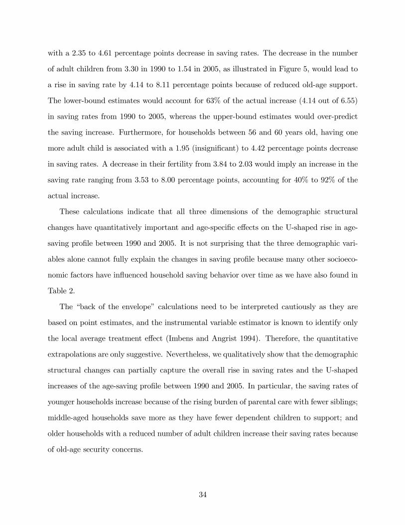
with a 2.35 to 4.61 percentage points decrease in saving rates. The decrease in the number
of adult children from 3.30 in 1990 to 1.54 in 2005, as illustrated in Figure 5, would lead to
a rise in saving rate by 4.14 to 8.11 percentage points because of reduced old-age support.
The lower-bound estimates would account for 63% of the actual increase (4.14 out of 6.55)
in saving rates from 1990 to 2005, whereas the upper-bound estimates would over-predict
the saving increase. Furthermore, for households between 56 and 60 years old, having one
more adult child is associated with a 1.95 (insignificant) to 4.42 percentage points decrease
in saving rates. A decrease in their fertility from 3.84 to 2.03 would imply an increase in the
saving rate ranging from 3.53 to 8.00 percentage points, accounting for 40% to 92% of the
actual increase.
These calculations indicate that all three dimensions of the demographic structural
changes have quantitatively important and age-specific effects on the U-shaped rise in age-
saving profile between 1990 and 2005. It is not surprising that the three demographic vari-
ables alone cannot fully explain the changes in saving profile because many other socioeco-
nomic factors have influenced household saving behavior over time as we have also found in
Table 2.
The “back of the envelope” calculations need to be interpreted cautiously as they are
based on point estimates, and the instrumental variable estimator is known to identify only
the local average treatment effect (Imbens and Angrist 1994). Therefore, the quantitative
extrapolations are only suggestive. Nevertheless, we qualitatively show that the demographic
structural changes can partially capture the overall rise in saving rates and the U-shaped
increases of the age-saving profile between 1990 and 2005. In particular, the saving rates of
younger households increase because of the rising burden of parental care with fewer siblings;
middle-aged households save more as they have fewer dependent children to support; and
older households with a reduced number of adult children increase their saving rates because
of old-age security concerns.
34

6 Conclusion
In this paper, to resolve the Chinese household saving puzzle, we have postulated and esti-
mated the effects of demographic changes on household saving in China. To this end, we have
studied China’s population policies. The population control policies substantially changed
the number of children Chinese households have. We exploit the variation in the changes in
fertility for households from several birth cohorts and across provinces to identify the effects
of demographic structural change on saving rates. The results indicate that demographic
structural changes have age-specific effects on household saving decisions. When we use the
estimated model to investigate the changes in household saving profile between 1990 and
2005, we find that younger households save more because of the rising burden of parental
care with fewer siblings. Middle-aged households save more as they have fewer dependent
children to support. Older households with a reduced number of adult children save more
because of old-age security concerns.
As the one-child policy approaches the third generation, the “4-2-1”type of family struc-
ture becomes more pervasive, that is, a family with one child, two parents, and four grand-
parents. One unanticipated consequence of the population control policies is perhaps the
increasing household saving. Our paper provides a new rationale for the relaxation of the
one-child policy: removing the birth quota could potentially stimulate household consump-
tion and substantially fuel current domestic demand.
35

References
Attanasio, Orazio P. (1998). “Cohort Analysis of Saving Behavior by U.S. Households.”
Journal of Human Resources, 33(3): 575—609.
Attanasio, Orazio P., and Agar Brugiavini (2003). “Social Security and Households’Saving.”
Quarterly Journal of Economics, 118(3): 1075—1119.
Banerjee, Abhijit, Xin Meng, and Nancy Qian (2010). “The Life Cycle Model and Household
Savings: Micro Evidence from Urban China.”Working paper, Yale University.
Chamon, Marcos, and Eswar Prasad (2010). “Why Are Saving Rates of Urban Households
in China Rising?”American Economic Journal: Macroeconomics, 2(1): 93—130.
Chen, Binkai, Ming Lu, and Ninghua Zhong (2012). “Hukou and Consumption Heterogene-
ity: Migrants’Expenditure is Depressed by Institutional Constraints in Urban China.”Work-
ing paper. Available at SSRN: http://ssrn.com/abstract=1989257 or http://dx.doi.org/10.2139/ssrn.1989257.
Coale, Ansley J. (1984). “Rapid Population Change in China, 1952—1982.”National Acad-
emy Press, Washington, D.C.
Curtis, Chadwick C., Steven Lugauer, and Nelson C. Mark (2011). “Demographic Patterns
and Household Saving in China.”Working paper, University of Notre Dame.
Ebenstein, Avraham (2010). “The ‘Missing Girls’ of China and the Unintended Conse-
quences of the One Child Policy.”Journal of Human Resources, 45(1): 87—115.
Gu, Baochang, Feng Wang, Zhigang Guo, and Erli Zhang (2007). “China’s Local and Na-
tional Fertility Policies at the End of the Twentieth Century.”Population and Development
Review, 33(1): 129—147.
Hesketh, Therese, Lu Li, and Wei Xing Zhu (2005). “The Effect of China’s One-Child Family
Policy after 25 Years.”New England Journal of Medicine, 353(11): 1171—1176.
36

Horioka, Charles Yuji, and Junmin Wan (2007). “The Determinants of Household Saving
in China: A Dynamic Panel Analysis of Provincial Data.” Journal of Money, Credit and
Banking, 39(8): 2077—2096.
Imbens, Guido W., and Joshua D. Angrist (1994). “Identification and Estimation of Local
Average Treatment Effects.”Econometrica, 62(2): 467—475.
Jappelli, Tullio, and Franco Modigliani (2005). “The Age-Saving Profile and the Life-Cycle
Hypothesis.”In The Collected Papers of Franco Modigliani, Volume 6. Cambridge, Massa-
chusetts: The MIT Press: 141-172.
Li, Hongbin, Junjian Yi, and Junsen Zhang (2011). “Estimating the Effect of the One-
Child Policy on Sex Ratio Imbalance in China: Identification Based on the Difference-in-
Differences.”Demography, 48(4): 1535—1557.
Li, Hongbin, and Junsen Zhang (2009). “Testing the External Effect of Household Behavior:
The Case of the Demand for Children.”Journal of Human Resources 44(4): 890—915.
Modigliani, Franco, and Shi Larry Cao (2004). “The Chinese Saving Puzzle and the Life-
Cycle Hypothesis.”Journal of Economic Literature, 42(1): 145—170.
Scharping, Thomas (2003). “Birth Control in China 1949—2000: Population Policy and
Demographic Development.”New York, NY: Routledge Curzon.
Short, Susan E., and Fengying Zhai (1998). “Looking Locally at China’s One-Child Policy.”
Studies in Family Planning 29(4): 373—387.
Song, Zheng, Kjetil Storesletten, Yikai Wang, and Fabrizio Zilibotti (2012). “Sharing High
Growth Across Generations: Pensions and Demographic Transition in China.” Working
paper, University of Zurich.
Song, Zheng, and Dennis Tao Yang (2010). “Life Cycle Earnings and Saving in a Fast-
Growing Economy.”Working paper, Chinese University of Hong Kong.
37

United Nations (2008). World Population Prospects, the 2008 Revision. Population Division,
Department of Economic and Social Affairs, United Nations. http://esa.un.org/unpp.
Wei, Shang-Jin, and Xiaobo Zhang (2011). “The Competitive Saving Motive: Evidence
from Rising Sex Ratios and Savings Rates in China.”Journal of Political Economy, 119(3):
511—564.
Yang, Dennis Tao, and Dandan Chen (2004). “Transformations in China’s Population Poli-
cies and Demographic Structure.”Pacific Economic Review, 9(3): 269—290.
Yang, Dennis Tao, Junsen Zhang, and Shaojie Zhou (2012). “Why Are Saving Rates So
High in China?”In Chapter 5 of Capitalizing China, edited by Joseph P. H. Fan and Randall
Morck. Chicago: University Of Chicago Press: 249-278.
38
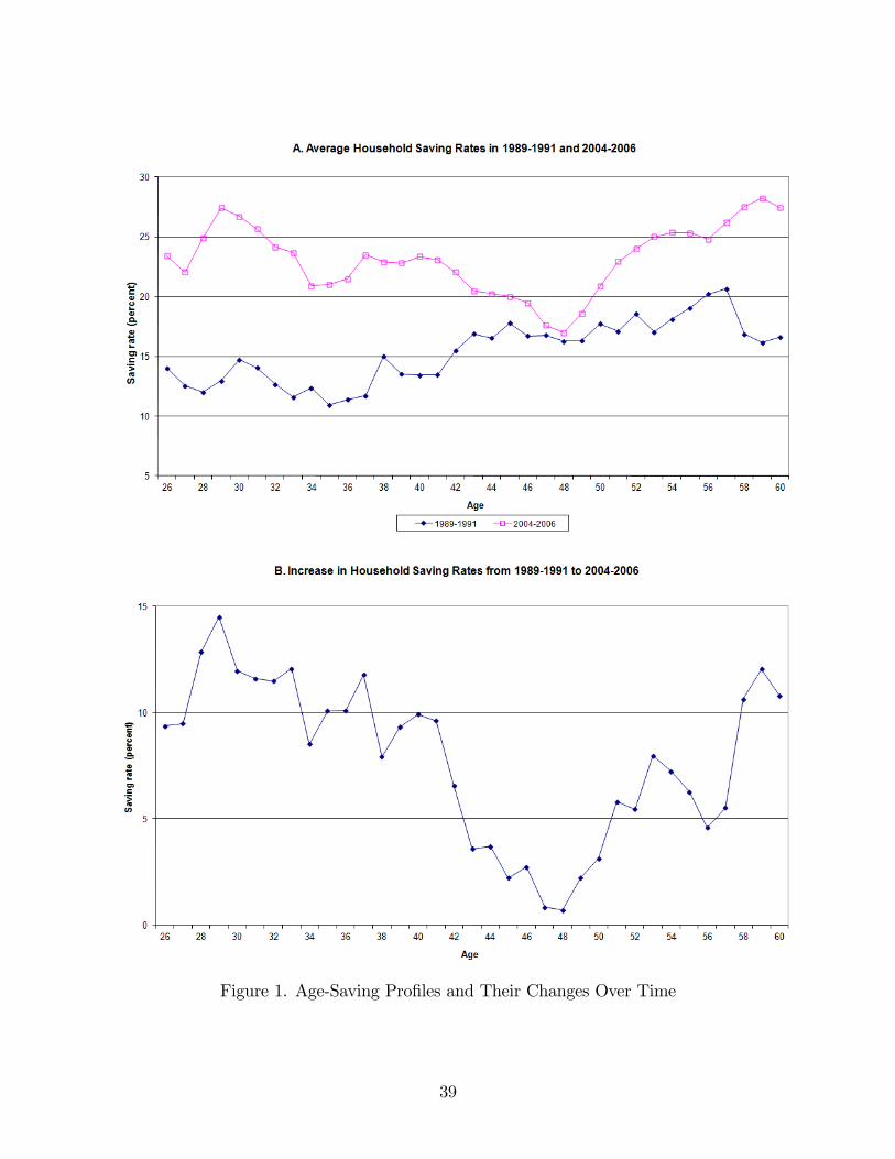
Figure 1. Age-Saving Profiles and Their Changes Over Time
39

0.0
10.0
20.0
30.0
40.0
50.0
60.0
70.0
80.0
1970 1975 1980 1985 1990 1995 2000 2005 2010 2015 2020 2025 2030 2035 2040 2045 2050
Young dependency ratio Old dependency ratio
Source: Population Division of the Department of Economic and Social Affairs of the United NationsSecretariat, World Population Prospects: The 2008 Revision, http://esa.un.org/unpp.
Figure 2. China’s Long-Term Population Trends: 1970 to 2050
40

1970
20 15 10 5 0 5 10 15 20
04
1014
2024
3034
4044
5054
6064
7074
8084
9094
100+Age
Female (%) Male (%)
1980
20 15 10 5 0 5 10 15 20
04
1014
2024
3034
4044
5054
6064
7074
8084
9094
100+Age
Female (%) Male (%)
1990
20 15 10 5 0 5 10 15 20
04
1014
2024
3034
4044
5054
6064
7074
8084
9094
100+Age
Female (%) Male (%)
2000
20 15 10 5 0 5 10 15 20
04
1014
2024
3034
4044
5054
6064
7074
8084
9094
100+Age
Female (%) Male (%)
2010
20 15 10 5 0 5 10 15 20
04
1014
2024
3034
4044
5054
6064
7074
8084
9094
100+Age
Female (%) Male (%)
2050
20 15 10 5 0 5 10 15 20
04
1014
2024
3034
4044
5054
6064
7074
8084
9094
100+Age
Female (%) Male (%)
Figure 3. Age Distribution of the Chinese Population: 1970 to 2050
41

Figure 4. Inter-Generational Links
42

Figure 5. Average Number of Children Profiles and Their Changes Over Time
43

Figure 6. Number of Dependent Children Profiles and Their Changes Over Time
44

Figure 7. Number of Siblings Profiles and Their Changes Over Time
45