Population Fluctuations in Ecosystems

Population Fluctuations in

Ecosystems

New Mexico

Supercomputing Challenge

Final Report

March 1, 2015

Team 4

Albuquerque Academy

Team Members: Carl Cherne

Mark Swiler

Jason Watlington

Mentor: Jim Mims

Population Fluctuations in Ecosystems

Page | 2

Table of Contents

1.0 Executive Summary

2.0 Problem Statement

3.0 Background Information

4.0 Procedural Overview

4.1 Algorithm

4.2 Visualization

5.0 Results

5.1 Control Results

5.2 Plant Variation Results

5.3 Primary Consumer Results

5.4 Predator Results

6.0 Conclusions

7.0 Future Work

8.0 Appendix

8.1 Appendix A: Average Control Run Graphs (Figures 1.00-1.11)

8.2 Appendix B: Plant Variable Changes (Figures 2.00-2.03)

8.3 Appendix C: Primary Consumer Variable Changes (Figures 3.00-3.06)

8.4 Appendix D: Predator Variable Changes (Figures 4.-4. )

8.5 Appendix E: Miscellaneous Figures (Figures 5.-5. )

8.6 Appendix F: Acknowledgements

8.7 Appendix G: Works Cited

3

4

5

7

7

10

11

12

14

15

16

19

21

23

23

29

31

34

37

39

39


Page | 3

1.0 Executive Summary

The interactions between organisms are the driving force for life on Earth. Some

of these interactions include the consumption of one organism by another,

reproduction between two members of the same species, and behaviors in movement.

In the broadest terms, we can classify organisms by their means of attaining nutrients

and energy. Producers are organisms that get energy from a direct source, be it

through photosynthesis or chemosynthesis. Consumers are organisms with a method of

locomotion that gain energy by eating other organisms. Primary consumers are

organisms which consume producers, whereas secondary consumers, or predators,

consume primary consumers, producers, or other secondary consumers.

Ecosystems are groups of organisms; analyzing an ecosystem means trying to

understand the different interactions that occur between the organisms it

encompasses. In this project, a set of behaviors for the member organisms will allow us

to see the overall behavior of the ecosystem. Our algorithm models three different

species of organisms: predators, primary consumers, and plants (producers). In the

report, we will refer to the predators, primary consumers, and plants as dinosaurs,

bigfeet, and plants respectively. These species all behave in unique ways, representing

animals and plants that we see on Earth. The algorithm we created uses an agent-

based model to help us understand how wild animal populations fluctuate; the

algorithm also delves into the effects of cataclysmic events. Understanding the effects

of human interaction upon a group of organisms will grow increasingly important in this

millennia; learning the differences between harmless, detrimental, and catastrophic

interactions may help protect the biodiversity we see on this planet.


Page | 4

2.0 Problem Statement

What intrinsic traits of an animal have the largest effect on the entire ecosystem?

Our model proposes an agent based model rather than existing equations to solve this.

At first, we were interested in looking at making each animal with different traits, but we

observed the data in our current model would be more meaningful than adding traits.

We wanted to know what happened to populations of each species over time. Would

every run result in the extinction of the predator species given enough time? Our goal

was to provide an accurate prediction of how species would change over time using

an agent based model.


Page | 5

3.0 Background Information

During World War I, fishing in the Mediterranean was sharply reduced to help

support the total war effort. When fishing resumed after the war ended, the fish

population had been decimated. A scientist named Vito Volterra attempted to

understand the cause of this enigma. He deduced that after the fish population was

left unchecked, the shark population began to thrive. Once the shark population

increased, it ravaged the local fish population. Volterra learned that populations follow

cyclical patterns of peaks and troughs; the fisherman resumed while the fish population

was experiencing a trough. Volterra also learned that the removal of a member of an

ecosystem greatly impacts the surrounding populations, destabilizing an ecosystem.

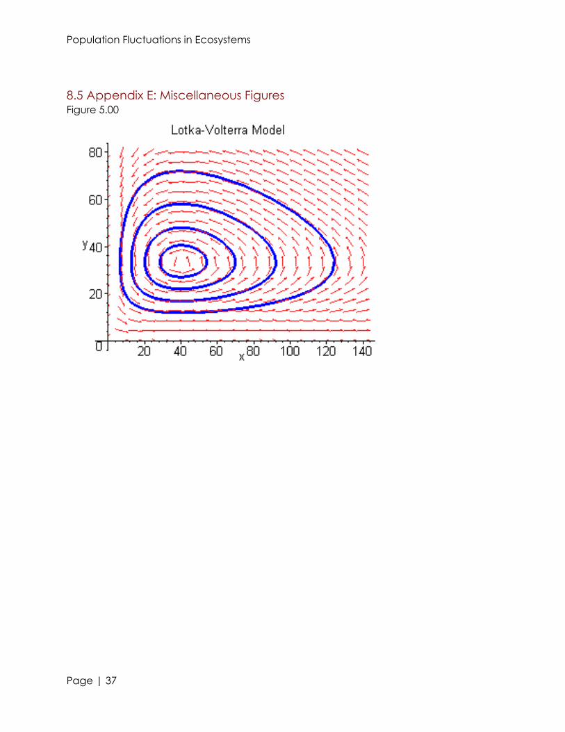
Simultaneous but exclusively, Volterra, and an American scientist, Alfred Lotka,

developed an equation which could help explain this change in populations. This

equation would later be known as the Lotka-Volterra equation. The first equation shows

that a true equilibrium is never established in an animal populations; the populations will

rise and fall in correlation to the abundance of their food. This equation works well for

the ecosystem that we are modeling, where there is a plethora of food and the

predator only relies on one (or very similar) species of prey. The basic equation changes

when food is not so plentiful so the prey are spread out. A new term is added that

involves the capacity and density of the prey, so there is no result in a situation in which

the predators can survive sustainably. This explains why places like Australia have an

ecosystem in which the greatest amount of predators are large reptiles, like snakes,

because they have greater efficiency in extracting energy from their food. See figure

5.00 for a graphical demonstration of this concept.


Page | 6

The Lotka-Volterra equations can be easily modified to model much more than

just predators and prey. Many events in life have a periodic sequence which relies on

the value of the other party, and is independent of time. One of these is love between

two people, the “Romeo and Juliet” model. This model is between two people, where

Romeo’s love increases with Juliet’s, but Juliet’s decreases as Romeo’s increases. This

will produce a periodic graph similar to the Predator prey model. This is also seen in

models of Guerilla warfare, where the strength does not solely rely on the sheer number

of either force because they can hide in buildings, but the casualties of each side are

proportional to both their own numbers and the opponent’s numbers. So if one side

has less men, they will also die less, because they can hide more easily and cannot all

be shot at once, like open warfare.

Although an equation such as the Lotka-Volterra model can roughly estimate

the populations of animals and show the general cyclical behavior of the ecosystem, it

does not take into account many minute factors which can greatly impact an

organism’s population. These factors all pertain to the traits and behaviors of individual

organisms and species, as each organism is its own entity which acts on its own accord.

When examining actual data of populations in ecosystem, you can draw trends from

the minutest of scales, such as months, to the greatest amounts of time, such as millions

of years. As you expand your analysis of ecosystems onto a longer, broader scale,

trends can become more esoteric; as there are a massive number of species which

interact with each other, and the cause of extinctions or population inflations can seem

uncaused. However, one thing is certain: all ecosystems follow periodic trends.


Page | 7

4.0 Procedural Overview

4.1 Algorithm

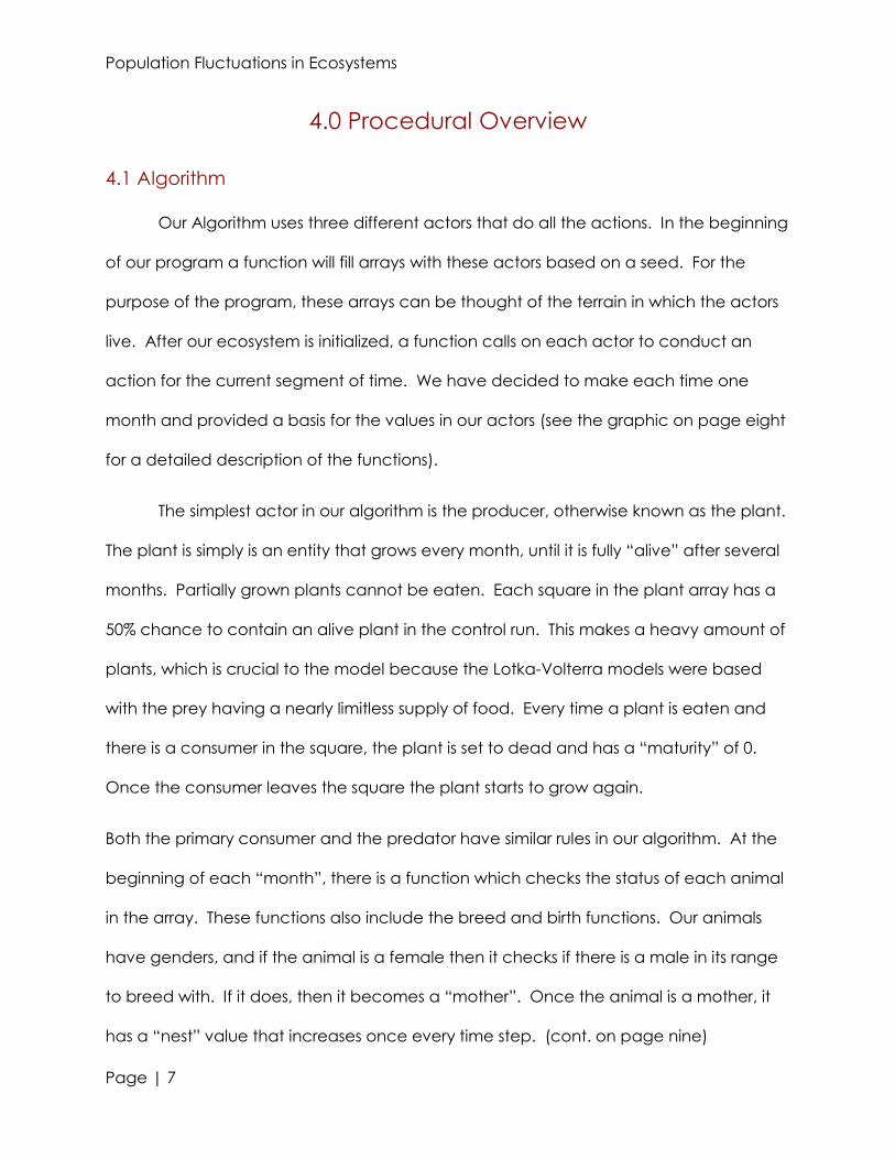
Our Algorithm uses three different actors that do all the actions. In the beginning

of our program a function will fill arrays with these actors based on a seed. For the

purpose of the program, these arrays can be thought of the terrain in which the actors

live. After our ecosystem is initialized, a function calls on each actor to conduct an

action for the current segment of time. We have decided to make each time one

month and provided a basis for the values in our actors (see the graphic on page eight

for a detailed description of the functions).

The simplest actor in our algorithm is the producer, otherwise known as the plant.

The plant is simply is an entity that grows every month, until it is fully “alive” after several

months. Partially grown plants cannot be eaten. Each square in the plant array has a

50% chance to contain an alive plant in the control run. This makes a heavy amount of

plants, which is crucial to the model because the Lotka-Volterra models were based

with the prey having a nearly limitless supply of food. Every time a plant is eaten and

there is a consumer in the square, the plant is set to dead and has a “maturity” of 0.

Once the consumer leaves the square the plant starts to grow again.

Both the primary consumer and the predator have similar rules in our algorithm. At the

beginning of each “month”, there is a function which checks the status of each animal

in the array. These functions also include the breed and birth functions. Our animals

have genders, and if the animal is a female then it checks if there is a male in its range

to breed with. If it does, then it becomes a “mother”. Once the animal is a mother, it

has a “nest” value that increases once every time step. (cont. on page nine)


Page | 8

Initialize

• This initializes the plant, then the bigfoot, and finally the dinosaur array

• For each species, If a random number between 1-100 is less than the "Initial value," an object of that type is placed there

Life check

• Each bigfoot and dinosaur go through a series of chencks at the beginning of the timestep

• First it will check to see if the animal is a mother, and if it can give birth

• If not , it will try to breed if it is a female

• After that it will check its age, and it will die if it is older than the maximum

• Finally, it will check to see how hungry it is, and it will die if it hasn't eaten in a certain period of time

Bigmeal

• This is how a bigfoot eats

• If there is a plant in the range it will place that square in a possible square

• The bigfoot will randomly choose one of the squares with a plant on it

• This takes up its movement, preventing it from eating more than once

Plant regen

• Every plant will grow in maturity if there is not a bigfoot there

• If the plant reaches a certain maturity, it can now be eaten by a bigfoot

Dinomeal

• Very similar to the bigmeal except for dinosaurs to eat bigfeet

• In addition, the dinosaur will move to a random square next to it if cannot find any bigfeet

• Unlike the plants, bigfeet have a chance to escape from being eaten


Page | 9

The breed function is called once the nest value is equal to the gestation value. This

function will create a new animal in a consecutive square that is randomly decided.

Then a consumer will check for any living plants without a predator in them. Since a

predator only eats consumers, they can be located on the same square as a plant,

while a consumer must be on its own square. After the consumers move the plants

regenerate, then the predators will eat. Each animal has a large range of 7*7 since

they will die so fast if they cannot find food. There are checks to make sure each

animal can only move once per time step. Each animal will automatically die if they

do not eat or they reach a certain age. It is important to note that there are three

separate arrays, and each object does not directly interact with an actor from another

array.

Another feature we used in creating and collecting data were input/output files.

Altogether we ran over 100 trials with different parameters, so these files allowed us to

quickly run our program without recompiling it every time. It also placed the data in a

spreadsheet where it could be graphed and organized.

4.2 Visualization

When using a small ten by ten or twelve by twelve grid, we visualized our

simulation simply using the command prompt. This proved very helpful when

debugging, because we labeled each individual so we could tell if it was moving more

than once. We represented each space in the grid by a horizontal bar to separate

elements in the row, and nothing to separate elements in a column. A plant is a P, a

Bigfoot is a B, and a dinosaur is a D. A dinosaur and a plant located on the same

square is represented by a H. However, these dimensions are too small to give good


Page | 10

results due to the behavior of the predators, and the results we gathered were by using

a grid two hundred by two hundred. See figure 5.01 for an example of this

visualization. Note, that on the final code, we have omitted these functions for greater

efficiency.


Page | 11

5.0 Results

In our program, there are two global variables which we didn’t change while

collecting data. The first is the seed value; we used zero for this, which provides a new,

random seed upon every run. Also, we didn’t change the run length of 3000 iterations.

In this model, every iteration roughly represents a month. However, our program has 11

global variables which we altered in order to see how they would affect the ecosystem:

Initial Values (Plant, Primary Consumer, Predator)

These values help determine the initial percentage of the ecosystem’s

space that is covered by either plants, primary consumers, or predators.

Age (Plant, Primary Consumer, Predator)

In the case of primary consumers and predators, these values place a

limit on how many iterations they can survive before they are forced to

die. Generally, these entities will die because of starvation or being

eaten, but this helps ensure that they do not remain in the ecosystem for

an unrealistic amount of time.

In the case of plants, the age variable determines how many iterations it

takes for a forested square to completely regrow.

Hunger (Primary Consumer, Predator)

The hunger variable determines how many iterations a primary consumer

or predator can survive without food before starving. This value cannot

be changed a significant amount, because in general, animals cannot

survive for more than a month without eating.

Gestation periods (Primary Consumer, Predator)

Gestation periods determine how many iterations a “pregnant” primary

consumer or predator will take until they birth a single offspring.

Defense (Primary Consumer)

The defense variable represents the percent chance of a primary

consumer surviving an attack by a predator.


Page | 12

5.1 Control Model

Parameters:

Our control model used parameters that we thought were representative of a

realistic ecosystem in its simplest form:

Seed Value: 0

Initial Value Plants: 50%

Initial Value Bigfeet: 25%

Initial Value Dinosaurs: 2%

Plant Age: 5 Iterations (5 months)

Primary Consumer Age: 84 Iterations (7 years)

Predator Age: 168 Iterations (14 Years)

Primary Consumer Hunger: 1 Iteration (1 month)

Predator Hunger: 1 Iteration (1 month)

Primary Consumer Gestation: 3 Iterations (3 months)

Predator Gestation: 6 Iterations (6 months)

Run length: 3000 Iterations (250 years)

Defense: 0%

Results:

The control code was ran 50 times, which helped us distinguish some patterns.

We averaged the 50 runs, and were able to create several graphs which help show

trends in the data( see figures 1.00-1.11 on Appendix 8.1 for graphs of the averages).

With the control code, we are generally able to find a relative equilibrium

between the species. As previously stated in the report, a true equilibrium is never

established, as the populations of predator, prey, and producer, cyclically increase and

decrease. However, after a certain period of time, we find that almost all data points

end up in a tight area which we call the “relative equilibrium”. This term means that all

of the organisms’ populations vacillate in a very minor fashion, as opposed to the

beginning of the ecosystem which sees great change.


Page | 13

Because of the random nature of the program, we can find variation between

the different runs. For example, in three of the 50 runs, we saw the extinction of the

predator species at 555, 796, and 906 iterations in, respectively. If you consider

extinction the existence of only one dinosaur, then the extinctions occur at 475, 655,

and 899 iterations. In the first case, it is apparent that the age limit prevented the final

dinosaur from living an absurdly long time, as it could find a high concentration of food

with no competition. In the second case, it is likely that the final dinosaur became

pregnant before the second to last dinosaur died, and gave birth before it died. Its

offspring eventually either died of age or starved.

Although the dinosaur populations occasionally die out, in no run did the bigfoot

population die out. This is not representative of the real world, and is likely due to the

overwhelming forestation.

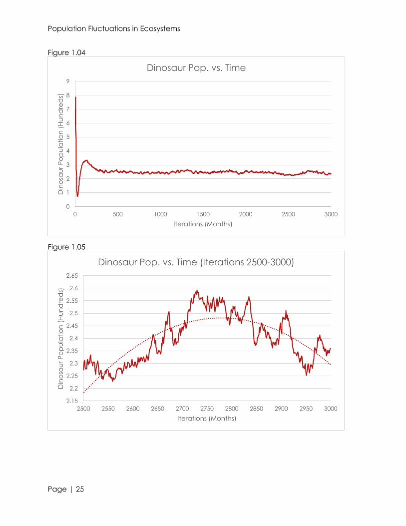
On a macro scale, once a relative equilibrium is reached, we are able to see

very minute changes in the organism’s populations (see figures 1.00, 1.02, and 1.04).

However, on a micro scale, we are able to see fluctuations in the population of the

animals. By examining the averages of iterations 2500-3000, we are able to find

relationships between predator, prey, and producers (see figures 1.01, 1.03, and 1.05).

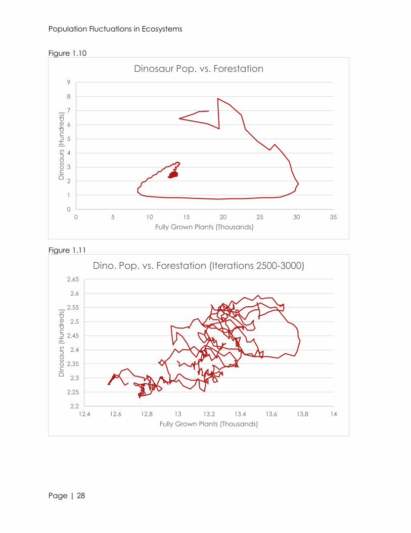
Ignoring the smaller troughs and peaks, we can see a rough, parabolic trend within the

500 iterations. For forestation and dinosaurs, we see a relative maxima in population at

approximately 2775 months in. With bigfeet, we see a relative minima at the same

time. This shows that in ecosystems, the populations of a predator and producer are

directly proportional; whereas the populations of a primary consumer are inversely


Page | 14

proportional to the previously stated two. When examining the graphs, we can see

that even the smallest peaks and troughs are correlated to eachother.

In sections 5.2-5.4, we experimented with the values of several variables, using

three runs for each change in a variable. For example, with plant age in 5.2, we used

values of three, four, six, and seven. For each of these variables, we ran three trials. This

resulted in 12 sets of data overall.

5.2 Variations in Producer

We experimented with the age value of the plants, using values of three, four, six,

and seven. Notice that five is omitted since it is the default value of the plant age. In

this context, the plant age value refers to the amount of months it takes for a plant to

become fully grown. Using three, four, and five (the default) values rarely provides

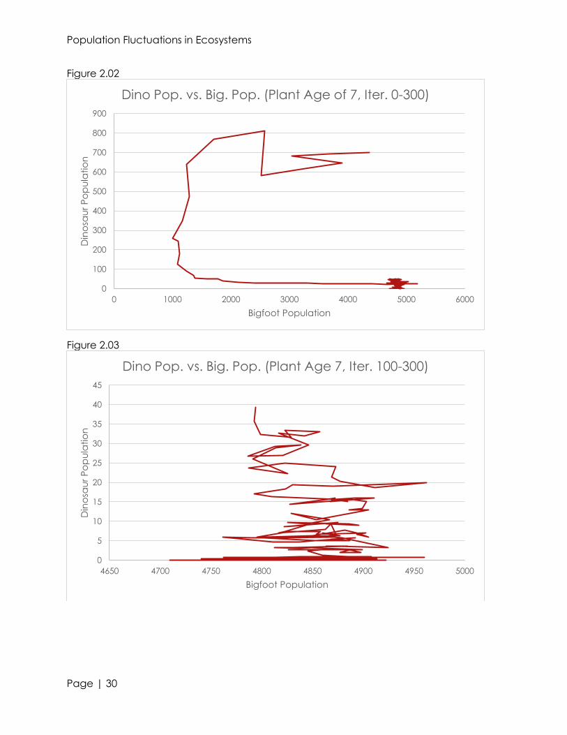
dinosaur extinctions. However, using a value of six or seven will results in dinosaur

extinctions nearly 100% of the time (see figures 2.00 and 2.01). This means that the

threshold of plant age which will result in 50% of extinctions within 3000 iterations is in

between five and six. With a value of six, we see extinction occur between 517 and 582

iterations. With a value of seven, we see extinction occur between 208 and 259

iterations. This is clearly caused by the direct correlation of dinosaur population to

forestation. If it takes longer for plants to fully develop and help stimulate the growth of

the bigfoot population, it affects the dinosaur population negatively.

We also changed the initial values of the plants, which determined how much of

the ecosystem was originally forested. This caused negligible change; the only

noticeable effect was that it took longer for the ecosystem to reach a relative

equilibrium.


Page | 15

5.3 Variations in Primary Consumer

With the primary consumer, we changed four different variables. These were

age, initial value, gestation, and defense chance. With age, we saw very little to no

change in the overall ecosystem. However, we did notice that, in general, an

increased age limit did result in a slightly more stable ecosystem. This means that the

relative maxima and minima once the system reached a relative equilibrium were

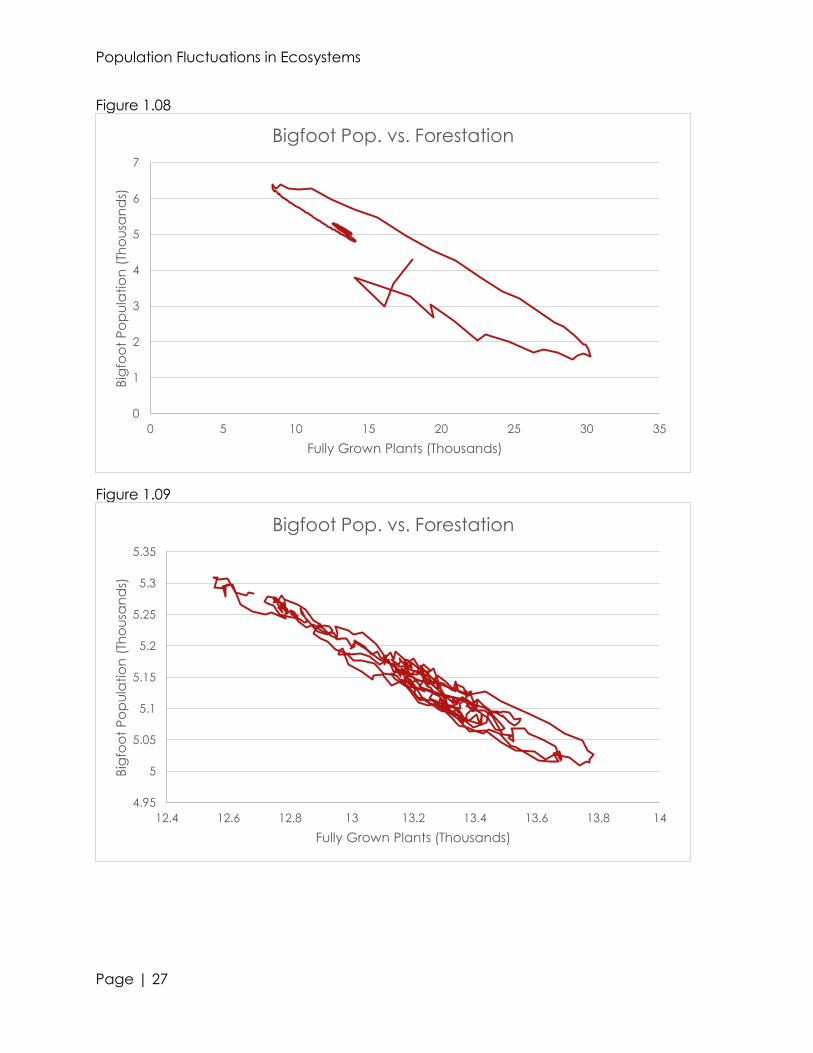
closer. The bigfoot population, as we previously discovered, is always stable; this is even

present after the dinosaur’s population has gone extinct. This is likely due to the

abundance of producer agents. Changing the initial values also caused very little

change, as only one of the results saw a dinosaur extinction—this was likely an outlier.

Changes in the gestation period of the bigfeet, however, saw a dramatic

change in the dinosaur population (see figures 3.00-3.03). By increasing the gestation

period of the bigfoot, the ecosystem saw a rapid decrease in the dinosaur population.

When the gestation period was four, one third of the ecosystems saw a dinosaur

extinction. With a gestation period of six, all ecosystems saw the extinction of dinosaurs

within 500 iterations. The graphs of gestation periods of eight and ten are almost

indistinguishably similar; in fact, a gestation period of eight iterations shows a quicker

extinction than a gestation period of ten iterations. This can be associated to two

causes: one, because of the random nature of the program; and two, because, after

increasing the gestation period past eight iterations, it is impossible for the dinosaur

population to survive. The dinosaur population, with a bigfoot gestation period of eight

or higher, survives until approximately 24 iterations due to a lack of food in the system to

sustain themselves.


Page | 16

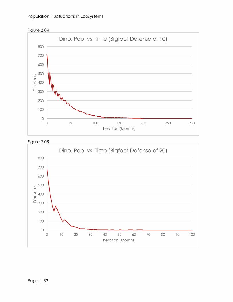
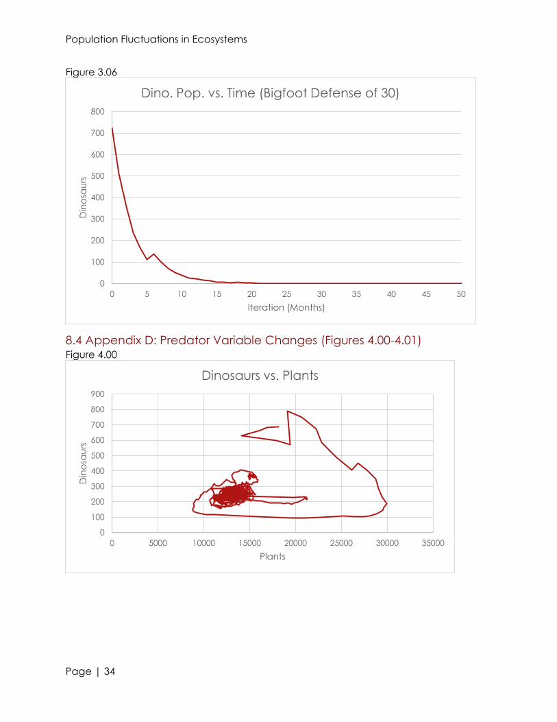
Altering the value of the defense chance also proved to cause great change in

the ecosystem. Even raising the chance of a bigfoot to defend themselves by 10% saw

the extinction of dinosaurs between 134 and 217 iterations. Further increasing the

chance for a bigfoot to defend itself caused an even earlier extinction of dinosaurs

(see figures 3.04-3.06). It is very interesting how even increasing the defense chance a

minute amount can immensely effect an ecosystem. This is because every interaction

between every species is related; if one dinosaur is denied food, and dies, it reduces

the probability that another dinosaur of the opposite sex could breed with it.

5.4 Variations in Predator

To investigate the dinosaur population, we changed three parameters:

Gestation period, starting populations, and maximum age. Each time a parameter was

changed, three runs were conducted, and the results for each one were the average

of all runs with that parameter. For the most part, we only graphed the population of

dinosaurs relative to plants and bigfeet because there was not an observable

correlation between the dinosaur population and time.

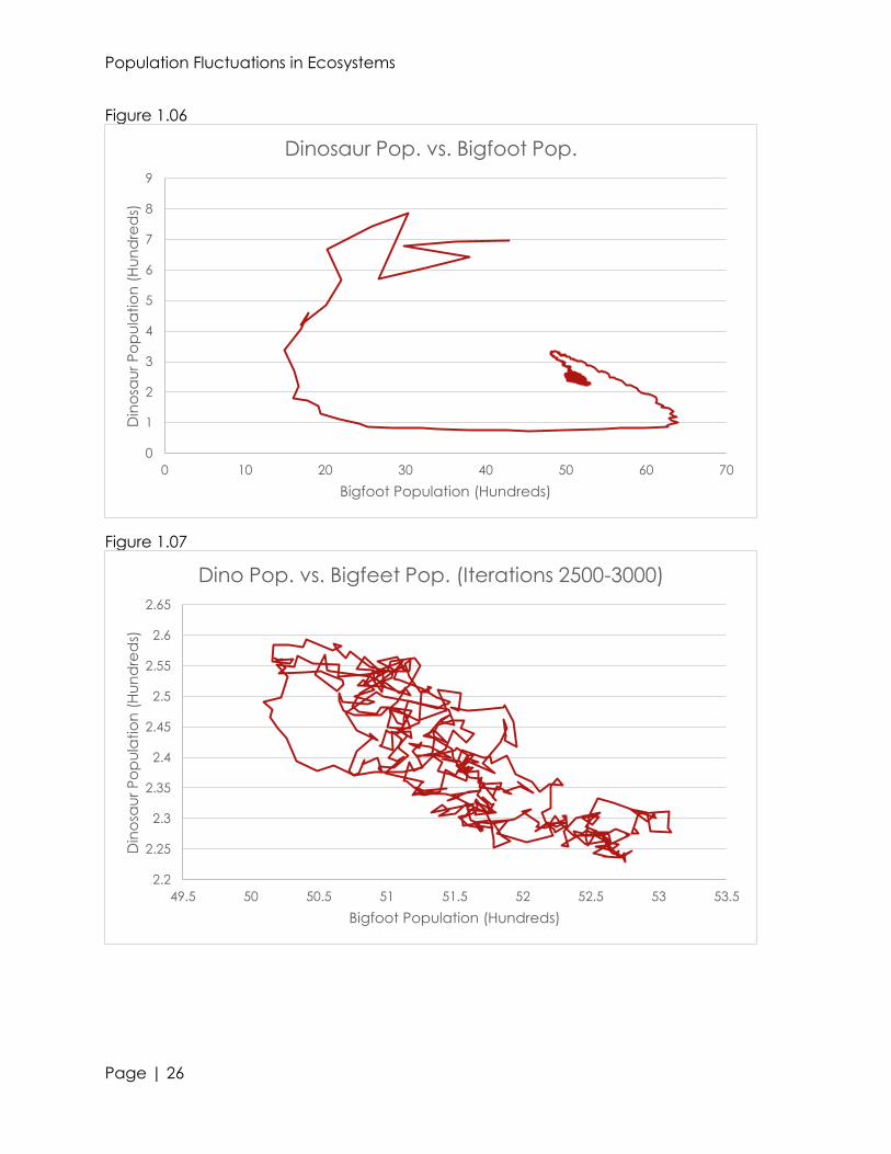
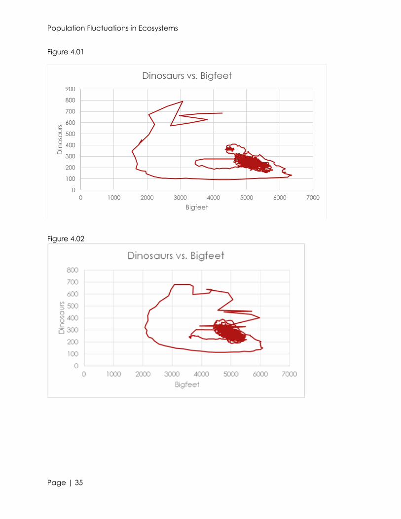
Most of our results followed similar patterns even with different parameters. The

first few months were understandably the most volatile, and often started with high

numbers of dinosaurs, and they quickly died as their prey disappeared. The system

started out like the Lotka-Volterra equations would suggest, but did not have the same

periodic cycle because it spiraled around a point (the center). An unexpected trend

that existed was the similarity between the dinosaur vs. plant and dinosaur vs. bigfoot

graphs (see figures 4.00 and 4.01). The graph with the plants as the x-axis was

essentially the graph of the bigfoot reflected with respect to the y-axis and

appropriately scaled. In fact, the plant graph followed the trend more closely than the


Page | 17

bigfoot graph. This means that we can accurately estimate populations of the bigfoot

species at a point in time if we have the plant graph.

Almost all of the graphs had one smaller loop that sprung out straight to the left

of the center. This is the same shape as demonstrated by the Lotka-volterra equations.

The dinosaurs reach a population where they will quickly eat a lot of bigfeet without a

decline in their own population. Then comes a point when the dinosaurs are impacted

by the lower bigfoot population, and drop nearly straight down. The bigfoot

population will steadily recover without changing the dinosaur population. Once the

bigfoot population recovers to what is was before, the dinosaurs will slowly grow and

the cycle will happen again. This cycle is constantly happening, but is only noticeable

once or twice because after that it will happen on a smaller scale and closer to the

center so all the points are clustered densely together and each period of the cycle is

indistinguishable from the next.

Changing the gestation period resulted in small but important differences on the

ecosystem. Our control run had a gestation value of 6, and the maximum and

minimum values tested were 4 and 8. When the value was 4, the dinosaurs had a

relatively straightforward decline, but had more fluctuation in their populations. This

means the area around the center was more spread out than the control. The longer

gestation period resulted in less average dinosaurs, and therefore, more average

bigfeet. As the gestation period grew longer, the beginning of the run became more

unpredictable and chaotic, but the area around the center became more

concentrated. This happens because the dinosaurs are unable to give birth in the first

few months because of the longer gestation period, so the beginning is more

unpredictable. After the dinosaurs give birth, because there are fewer population


Page | 18

spikes that result from shorter gestation periods. The center hovered around 250

dinosaurs, 5,250 bigfeet, and 13,000 plants when the value was 8. However, when the

value is 4 the center changes to around 300 dinosaurs, 4,750 bigfeet, and 15,000 plants.

Changing the initial value produced the greatest effects on the ecosystem. The initial

value of one produced the graph that was smoothest and appeared most like the

Lotka graph. This is because there were fewer dinosaurs to begin with, so the system

experienced fewer shocks in the beginning.

When the initial value was increased to two, the populations became more

unpredictable and jumped around more in the beginning months. However, when the

initial value changed to three, a sharp contrast occurred (see figures 4.02 and 4.03).

There were so many dinosaurs at the beginning that many died of hunger and could

not recover enough to survive. The dinosaurs died around month 1200, but they stayed

under 20 individuals since the 900th month. Because we used a random seed, not every

run will result in the dinosaur’s extinction, but it is a stark difference from the initial value

of two, when there is almost a 0% chance of extinction. When the initial value was

further increased to four the dinosaurs died even more quickly, in only about 200

months.

The age component affected the overall outcome the least of the variables we

changed. This happened for two reasons. Firstly, since they will die if they do not eat

for one month, they will mostly all die from hunger rather than age. Secondly, while we

doubled the gestation period from four to eight and quadrupled the initial values from

one to four, the increase from 144 to 192 is only 33%. Essentially we are deviating less

from our control run with our age tests.


Page | 19

6.0 Conclusions

Establishing a stable ecosystem using our algorithm can be a complicated task.

Even the slightest change in the parameters for our ecosystem saw drastic change. It

was easiest to see the effects of a parametric variation by examining the population of

the dinosaur class. This is because plants do not have any requirements to grow, other

than an empty space in the ecosystem. Also, plants do not have an age limit;

therefore, plants will never go extinct in our ecosystem. Because of this abundance of

food, bigfeet populations will fluctuate, but not as violently as that of the dinosaur

population. Only in our earlier algorithms did bigfeet go extinct. However, dinosaur

populations often go extinct, due to a slight drop in the bigfoot population. Food

becomes scarce enough to the point where the dinosaur population cannot sustain

itself (see figures 2.02 and 2.03). Although the bigfeet are able to sustain themselves,

they do see a dip in population. This causes the dinosaur population to dramatically

dip, and eventually reach extinction. The extinction of this predator class does have a

great effect on the bigfoot population. In figure 2.03, you can see that near the

extinction of the dinosaur class, the bigfoot population sharply increases and

decreases. This can be attributed to the removal of a population check—in a way, this

is very similar to the Italian fish populations, which were greatly destabilized upon the

removal of a predator.

Although our algorithm is not perfect, it does display the volatility of the

ecosystems we find on earth. The effects of human behaviors such as overfishing,

urbanization, and pollution can greatly destabilize a local ecosystem. As Volterra was

able to see, ecosystems may also adapt to human interaction and become stable


Page | 20

because of activities such as hunting or fishing. A sudden removal of this interaction

can cause the destabilization of the ecosystem, which is the reason that the fish

population In Italy after WWI was greatly reduced. Even our simple algorithm shows just

how complicated ecosystems can become due to the amount of interactions

between species. Being able to forecast how different human interactions will affect

an ecosystem will become of increasing importance in the 21st century.


Page | 21

7.0 Future Work

Due to the open ended nature of our code, there are many areas for

improvement that we have recognized, and taken an interest in. However, we have

not committed to developing any of the proposed code which follows.

With this model, there is a tremendous amount of room for expansion. Originally,

we wanted to see how a dominant trait would emerge in an ecosystem due to the

surrounding environment and other animal populations. For the sake of simplicity, we

omitted both traits and environment from the final model in favor of examining the

changes that occur in animal populations. We were also interested in seeing the

effects of events, such as deforestation, on an animal population.

We also saw that the movement patterns of animals had a great effect upon the

stability of the ecosystem. We programmed the predators and primary consumers to

value tiles which had food on them higher than tiles which were void of food. However,

for a period of time, we only allowed the animals to see within a square of their tile.

During this time period, we saw that dinosaurs often went extinct very early in the life of

the ecosystem; within 100 iterations. However, after increasing the range of their ability

to find food, we saw that the organisms found a relative equilibrium much more often.

These changes were included in our control code. However, behaviors in movement

within animals are highly complicated, and unique often times. It would be very

interesting to implement these behaviors and see the effects on the ecosystems.

Our model is also very simple, in that we only use three species. In real

ecosystems, thousands of species from all kingdoms are present. While modeling

individual bacterium would be near impossible, decomposition on a broad scale could


Page | 22

be implemented to help check the growth of plants. Including different kinds of

animals in our ecosystem, such as omnivorous consumers, could help increase the

realism of the model. Adding several different species would be possible, but by doing

this, we would likely want to increase the space of the ecosystem. Since our PCs were

not able to run an array larger than 210 by 210, this would be an excellent task for a

supercomputer.


Page | 23

8.0 Appendix

8.1 Appendix A: Average Control Run Graphs (Figures 1.00-1.11) Figure 1.00

Figure 1.01

0

5

10

15

20

25

30

35

0 500 1000 1500 2000 2500 3000

Fu

lly G

row

n P

lan

ts (

Tho

usa

nd

s)

Iterations (Months)

Forestation vs. Time

12.4

12.6

12.8

13

13.2

13.4

13.6

13.8

14

2500 2550 2600 2650 2700 2750 2800 2850 2900 2950 3000

Fu

lly G

row

n P

lan

ts (

Tho

usa

nd

s)

Iterations (Months)

Forestation vs. Time (Iterations 2500-3000)


Page | 24

Figure 1.02

Figure 1.03

0

1

2

3

4

5

6

7

0 500 1000 1500 2000 2500 3000

Big

foo

t P

op

ula

tio

n (

Tho

usa

nd

s)

Iterations (Months)

Bigfoot Pop. vs. Time

4.95

5

5.05

5.1

5.15

5.2

5.25

5.3

5.35

2500 2550 2600 2650 2700 2750 2800 2850 2900 2950 3000

Big

foo

t P

op

ula

tio

n (

Tho

usa

nd

s)

Iterations (Months)

Bigfoot Pop. vs. Time (Iterations 2500-3000)


Page | 25

Figure 1.04

Figure 1.05

0

1

2

3

4

5

6

7

8

9

0 500 1000 1500 2000 2500 3000

Din

osa

ur

Po

pu

latio

n (

Hu

nd

red

s)

Iterations (Months)

Dinosaur Pop. vs. Time

2.15

2.2

2.25

2.3

2.35

2.4

2.45

2.5

2.55

2.6

2.65

2500 2550 2600 2650 2700 2750 2800 2850 2900 2950 3000

Din

osa

ur

Po

pu

latio

n (

Hu

nd

red

s)

Iterations (Months)

Dinosaur Pop. vs. Time (Iterations 2500-3000)


Page | 26

Figure 1.06

Figure 1.07

0

1

2

3

4

5

6

7

8

9

0 10 20 30 40 50 60 70

Din

osa

ur

Po

pu

latio

n (

Hu

nd

red

s)

Bigfoot Population (Hundreds)

Dinosaur Pop. vs. Bigfoot Pop.

2.2

2.25

2.3

2.35

2.4

2.45

2.5

2.55

2.6

2.65

49.5 50 50.5 51 51.5 52 52.5 53 53.5

Din

osa

ur

Po

pu

latio

n (

Hu

nd

red

s)

Bigfoot Population (Hundreds)

Dino Pop. vs. Bigfeet Pop. (Iterations 2500-3000)


Page | 27

Figure 1.08

Figure 1.09

0

1

2

3

4

5

6

7

0 5 10 15 20 25 30 35

Big

foo

t P

op

ula

tio

n (

Tho

usa

nd

s)

Fully Grown Plants (Thousands)

Bigfoot Pop. vs. Forestation

4.95

5

5.05

5.1

5.15

5.2

5.25

5.3

5.35

12.4 12.6 12.8 13 13.2 13.4 13.6 13.8 14

Big

foo

t P

op

ula

tio

n (

Tho

usa

nd

s)


Bigfoot Pop. vs. Forestation


Page | 28

Figure 1.10

Figure 1.11

0

1

2

3

4

5

6

7

8

9

0 5 10 15 20 25 30 35

Din

osa

urs

(H

un

dre

ds)


Dinosaur Pop. vs. Forestation

2.2

2.25

2.3

2.35

2.4

2.45

2.5

2.55

2.6

2.65

12.4 12.6 12.8 13 13.2 13.4 13.6 13.8 14

Din

osa

urs

(H

un

dre

ds)


Dino. Pop. vs. Forestation (Iterations 2500-3000)


Page | 29

8.2 Appendix B: Plant Variable Changes (Figures 2.00-2.03) Figure 2.00

Figure 2.01

0

1

2

3

4

5

6

7

8

9

0 100 200 300 400 500 600

Din

osa

ur

Po

pu

latio

n (

Hu

nd

red

s)

Iteration (Months)

Dinosaur Pop. vs. Time (Plant Age Value of 6)

0

1

2

3

4

5

6

7

8

9

0 100 200 300 400 500 600

Din

osa

ur

Po

pu

latio

n (

Hu

nd

red

s)

Iteration (Months)

Dinosaur Pop. vs. Time (Plant Age Value of 7)


Page | 30

Figure 2.02

Figure 2.03

0

100

200

300

400

500

600

700

800

900

0 1000 2000 3000 4000 5000 6000

Din

osa

ur

Po

pu

latio

n

Bigfoot Population

Dino Pop. vs. Big. Pop. (Plant Age of 7, Iter. 0-300)

0

5

10

15

20

25

30

35

40

45

4650 4700 4750 4800 4850 4900 4950 5000

Din

osa

ur

Po

pu

latio

n

Bigfoot Population

Dino Pop. vs. Big. Pop. (Plant Age 7, Iter. 100-300)


Page | 31

8.3 Appendix C: Primary Consumer Variable Changes (Figures 3.00-3.06) Figure 3.00

Figure 3.01

0

100

200

300

400

500

600

700

800

0 500 1000 1500 2000 2500 3000

Din

osa

ur

Po

pu

latio

n

Iteration (Months)

Dino. Pop. vs. Time (Bigfoot Gestation of 4)

0

100

200

300

400

500

600

700

800

0 100 200 300 400 500 600

Din

osa

ur

Po

pu

latio

n

Iteration (Months)



Page | 32

Figure 3.02

Figure 3.03

0

100

200

300

400

500

600

700

800

0 10 20 30 40 50 60 70 80 90 100

Din

osa

ur

Po

pu

latio

n

Iteration (Months)


0

100

200

300

400

500

600

700

800

0 10 20 30 40 50 60 70 80 90 100

Din

osa

ur

Po

pu

latio

n

Iteration (Months)



Page | 33

Figure 3.04

Figure 3.05

0

100

200

300

400

500

600

700

800

0 50 100 150 200 250 300

Din

osa

urs

Iteration (Months)

Dino. Pop. vs. Time (Bigfoot Defense of 10)

0

100

200

300

400

500

600

700

800

0 10 20 30 40 50 60 70 80 90 100

Din

osa

urs

Iteration (Months)



Page | 34

Figure 3.06

8.4 Appendix D: Predator Variable Changes (Figures 4.00-4.01) Figure 4.00

0

100

200

300

400

500

600

700

800

0 5 10 15 20 25 30 35 40 45 50

Din

osa

urs

Iteration (Months)


0

100

200

300

400

500

600

700

800

900

0 5000 10000 15000 20000 25000 30000 35000

Din

osa

urs

Plants

Dinosaurs vs. Plants


Page | 35

Figure 4.01

Figure 4.02

0

100

200

300

400

500

600

700

800

900

0 1000 2000 3000 4000 5000 6000 7000

DIn

osa

urs

Bigfeet

Dinosaurs vs. Bigfeet


Page | 36

Figure 4.03

Figure 4.04


Page | 37

8.5 Appendix E: Miscellaneous Figures Figure 5.00


Page | 38

Figure 5.01


Page | 39

8.6 Appendix F: Acknowledgements We would like to thank Tom Swiler for his assistance during the coding of this

project, and Jim Mims for putting in extra time to assist us with our presentations. Also,

we would like to thank the judges of the Supercomputing Challenge for giving us

constructive criticism which helped us improve our project and give us clearer goals.

8.7 Appendix G: Works Cited

Hamilton, William J., III. Mechanisms of Animal Behavior. New York: John Wiley & Sons,

1966. Print.

Morse, Douglass H. Behavioral Mechanisms in Ecology. Cambridge: Harvard UP, 1980.

Print.

Predator Prey Models." Predator Prey Models. Duke University, 10 July 2001. Web. 15 Mar.

2015.

<https://www.math.duke.edu/education/webfeats/Word2HTML/Predator.html>.

Roy, Peter Martin. The Living Plant. 2nd ed. New York: Holt, Rinehart and Winston, n.d.

Print. Modern Biology Series.

Slobodkin, Lawrence B. A Citizen's Guide to Ecology. Oxford: Oxford University Press,

2003. Print.

Tung, K. K. Topics in Mathematical Modeling. Princeton: Princeton UP, 2007. Print.

White, Gary C. "Modeling Population Dynamics." 6 May 1998. PDF file.

Documents

Population Fluctuations in Ecosystems