Pollution Control Policies and Natural Resource Dynamics: A Theoretical Analysis

Rinaldi, S., Sanderson, W.C. and Gragnani, A.

IIASA Working Paper

WP-95-108

October 1995

Rinaldi, S., Sanderson, W.C. and Gragnani, A. (1995) Pollution Control Policies and Natural Resource Dynamics: A

Theoretical Analysis. IIASA Working Paper. IIASA, Laxenburg, Austria, WP-95-108 Copyright © 1995 by the author(s).

http://pure.iiasa.ac.at/4488/

Working Papers on work of the International Institute for Applied Systems Analysis receive only limited review. Views or

opinions expressed herein do not necessarily represent those of the Institute, its National Member Organizations, or other

organizations supporting the work. All rights reserved. Permission to make digital or hard copies of all or part of this work

for personal or classroom use is granted without fee provided that copies are not made or distributed for profit or commercial

advantage. All copies must bear this notice and the full citation on the first page. For other purposes, to republish, to post on

servers or to redistribute to lists, permission must be sought by contacting repository@iiasa.ac.at

Working Paper Pollution Control Policies

and Natural Resource Dynamics: A Theoretical Analysis

Sergio Rinaldi Warren Sanderson

Alessandra Gragnani

WP-95- 108 October 1995

-1 lASA International Institute for Applied Systems Analysis A-2361 Laxenburg Austria

&mi: Telephone: +43 2236 807 Telefax: +43 2236 71 31 3 E-Mail: info@ iiasa.ac.at

Pollution Control Policies and Natural Resource Dynamics:

A Theoretical Analysis

Sergio Rinaldi Warren Sanderson

Alessandra Gragnani

WP-95- 108 October 1995

Working Papers are interim reports on work of the International Institute for Applied Systems Analysis and have received only limited review. Views or opinions expressed herein do not necessarily represent those of the Institute, its National Member Organizations, or other organizations supporting the work.

lASA International Institute for Applied Systems Analysis A-2361 Laxenburg Austria

DL 1. m m m w Telephone: +43 2236 807 Telefax: +43 2236 71 31 3 E-Mail: info@ iiasa.ac.at

About the Authors

Sergio Rinaldi is a professor at the Research Centre for Environmental and Computer Sciences (C.I.R.I.T.A), Politecnico di Milano, Milano, Italy.

Warren Sanderson is a senior research scholar in the Population Project at IIASA. He is on sabbatical leave from the Department of Economics, State University of New York at Stony Brook, Stony Brook, New York, U.S.A.

Alessandra Gragnani is a Ph.D. student, Department of Electronics and Information, Politecnico di Milano, Milano, Italy.

Acknowledgment

The research reported here was done at the International Institute for Applied Systems Analysis, Laxenburg, Austria, and partially supported by the Italian Ministry of Scientific Research and Technology, contract MURST 40% Teoria dei sistemi e del controllo.

Abstract

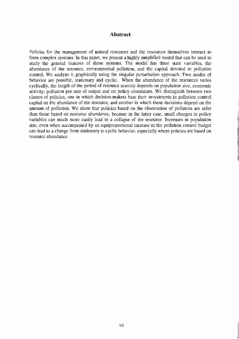
Policies for the management of natural resources and the resources themselves interact to form complex systems. In this paper, we present a highly simplified model that can be used to study the general features of those systems. The model has three state variables, the abundance of the resource, environmental pollution, and the capital devoted to pollution control. We analyze it graphically using the singular perturbation approach. Two modes of behavior are possible, stationary and cyclic. When the abundance of the resources varies cyclically, the length of the period of resource scarcity depends on population size, economic activity, pollution per unit of output and on policy constraints. We distinguish between two classes of policies, one in which decision-makers base their investments in pollution control capital on the abundance of the resource, and another in which those decisions depend on the amount of pollution. We show that policies based on the observation of pollution are safer than those based on resource abundance, because in the latter case, small changes in policy variables can much more easily lead to a collapse of the resource. Increases in population size, even when accompanied by an equiproportional increase in the pollution control budget can lead to a change from stationary to cyclic behavior, especially where policies are based on resource abundance.

vii

Table of Contents

1. Introduction

2. The Model

3. Environmental Dynamics with Constant Pollution Control Capital

4. Environmental Dynamics with Variable Pollution Control Capital

5. Influence of Economy and of Pollution Control Policy

6. Conclusions

Appendix

References

POLLLTTION CONTROL POLICIES AND NATURAL RESOURCE DYNAMICS: A THEORETICAL ANALYSIS

Sergio Rinaldi Warren Sanderson

Alessandra Gragnani

1. INTRODUCTION

Natural resources are not always in a stationary regime. Indeed, a number of resources

follow a cyclic regime, even when they are uncontaminated and unexploited. Recurrent pest

outbreaks, fires in Mediterranean forests, algal-blooms in water bodies are examples of

natural cycles. However, exploitation and contamination enrich the spectrum of possible

scenarios. Transitions from stationary to cyclic regimes, as well as collapses of a resource due

to a small increase of the exploitation effort or the concentration of a toxic substance are well

documented in fisheries, rangelands, aquatic and forest ecosystems. But the dynamics of the

resource becomes even more complex when exploitation and contamination vary in time.

Often the dynamics of the biological and chemical components (resources and contaminants)

of a given system influence the actions taken by institutions responsible for environmental

protection and exploitation. For example, progressive acidification of lakes and forests has

elicited a counteracting pollution control effort in a number of countries (United Nations

Economic Commission on Europe, 1994; International Institute for Applied Systems

Analysis, 1993).

Institutions and the economy interact with the environment, making the prediction of

the dynamics of the resulting system a highly complex problem (Walters, 1986). These

problems have been studied under many different circumstances and the models used share

many common features. In this paper, we present a simple general model that incorporates

some of the most important features and show how it can assist in policy formulation. In

particular, we consider the case of a resource growing in a contaminated environment, but

restrict our analysis by assuming that the economic activities that cause pollution flows are

not directly related to the resource or its exploitation.

The model has only three state variables: the abundance of the resource, environmental

pollution and the capital devoted to pollution control. It is simple in four ways. First, the

environmental system is composed of a unique resource influenced by one form of pollution

only. Interactions between different resources and/or between different pollutants are ignored.

Second, only two simple forms of pollution control policies are considered. Policy makers are

assumed to be ignorant of the details of the environmental system and are allowed to make

decisions only on the basis of information on the resource abundance or the pollution level.

Third, the socio-economic setting itself is highly simplified. Below, we consider how the

levels of those variables influence the system, but the dynamics of changes in the number of

people and pollution per person are ignored here. Fourth, the mathematics that we use to

identify the dynamics of the system is relatively simple. Indeed, all the properties that we

discuss are presented graphically, with the style used by Noy-Meir (1975) in his remarkable

paper on grazing systems.

The model is general in the sense that it is designed to capture the major features shared

by many environmental systems. Whenever possible, key relationships enter the model

through characterizations of their properties rather than through specific functional forms.

The result is a model that does not represent any specific system in full detail, but instead

incorporates the core features of many.

The main disadvantage of a simple and general model is that it cannot, by its nature,

produce new results for specific cases. Thus, virtually everything that we find has already

been found in the study of one or a number of specific resources. The prime advantage of this

approach is that we can see more clearly patterns that recur in the study of many resources

and that we can discuss policy formulation in a general context.

There have been four main approaches to the study of natural resources and they can be

described as entries in a two by two matrix. On one axis we have models that are analytic and

those that are specified numerically. On the other axis, we have models that characterize

policy decision rules with and without explicit optimization. (Notice that models that do not

explicitly make use of optimization may, nevertheless, take into account the rationality of the

agents involved.)

Numeric models with or without optimization (like linear programming models or

simulation models) are most often used to answer specific questions. In the case of

aquaculture, for example, Kishi et al. (1994) presents a management simulation model

applied to Mikame Bay in Japan, and Fisher et al. (1991) contains a model of a salmon

fishery in California. Such models are suitable for their own purposes, but lack the generality

that we seek here.

A good representative of the rich tradition of analytic models can be found in Clark

(1990) where exploitation policies are systematically derived through optimal control theory.

Those models provide us with certain insights. There are many cases, however, in which there

may be conflicting demands on the environmental system, so that a policy that is optimal

from one perspective may not be optimal from another. Second, and most important,

environmental systems may not be completely understood, so that it may be preferable to

follow a simple, pragmatic, but robust policy (that assumes little knowledge of the system),

than to follow a more complex policy derived through optimization, but based on an incorrect

assessment. This is in line with the tradition of process control engineering, where despite the

huge number of sophisticated criteria for designing optimal controllers, still the most

commonly used ones are the so-called industrial controllers. These controllers are very simple

and can be easily adapted to almost all situations, even if there is no clear understanding of

the dynamics of the process.

In this paper, we specify a priori the structure of the control policy, thus avoiding the

explicit use of any optimization criterion. This along with other simplifications produces an

analytically tractable model that allows us to derive general results in a very transparent way.

A purely geometric approach based on the singular perturbation m,ethod (Hoppensteadt,

1974; Muratori and Rinaldi, 1991) is used to show why and when the system will go to an

equilibrium or to a limit cycle and to point out the circumstances in which there will be

collapses and regenerations of the resource.

The results are:

( I ) There are two possible asymptotic modes of behavior: stationary or cyclic. The second

involves periodic collapses and regenerations of the resource, which take place in a short

period of time, and which are separated by relatively long periods of time during which the

resource is either abundant or scarce.

(2) The length of the period during which the resource is scarce sensitively depends on the

socio-economic setting, in particular population size, economic activity, pollution per unit of

output, and policy constraints.

(3) Pollution control policies based on observations of environmental pollution are safer

than those based on observation of the abundance of the resource, because the former are less

likely to lead to catastrophic collapses of the resource.

(4) Increasing population size, economic activity per capita or other parameters can cause

the system to change its behavior from stationary to cyclic. This is especially true in the case

where policy is based on resource abundance.

But, in a sense, the main result is that all the above properties are derived from a simple

and compact framework by using geometrical arguments only.

The model is presented in Section 2. We proceed with its analysis in three steps. In

Section 3, we consider the dynamics of resource abundance and environmental pollution for a

fixed amount of pollution control capital. The effects of using two classes of pollution control

policies on the dynamics of the whole system are shown in Section 4. In Section 5, we

describe the consequences of changes in population size, pollution per person, policy

constraints, and stocking. The final section contains concluding remarks.

2. THEMODEL

The model has only three variables. The first, R(t), is a measure of the abundance of the

resource at time t. Important biological characteristics of the resource, like species diversity,

age structure and sex ratio, as well as spatial inhomogeneity, are not considered here. The

second variable, P(t), is a measure of the environmental pollution that influences the growth

of the resource. The concentration of mobilized aluminum in the soil is a good example if the

resource is tree biomass. Another example is the concentration of filamentous cyanobacteria

(blue-green algae) if the resource is the amount of zooplankton supporting the fish stock in a

shallow lake. The third variable, C(t), is a measure of the capital devoted to pollution control

at time t per unit of potential pollution flow. The potential pollution flow, indicated by w, is

the flow of pollution that would be discharged into the environment in the absence of any

pollution control effort. For example, in the case of a lake surrounded by a number of towns

summing up to a population N, the potential pollution flow w would be N times the average

amount of pollution produced per person in one day. Thus C(t) would be the value of the

treatment plants active at time t divided by w. In other words, C(t) would be (modulo a

conversion factor) the pollution control capital per person used in treating wastewater.

Resource abundance, pollution and pollution control capital interact and vary over time

according to three simple differential equations:

where R , P and c are the time derivatives of R, P , and C, respectively.

The first term on the right-hand side of Eq. (1) is the basic logistic growth of the

resource. Net growth per capita and carrying capacity have been put equal to one. This is

always possible by suitably scaling time and the resource. The second term in that equation

represents surplus mortality due to pollution. M(P) is the excess mortality rate per capita and

it is assumed to be negligible up to a threshold and then to increase quite sharply as pollution

rises. In other words, M, M', and M" are non-negative. This is shown in Figure la , where the

threshold value of P has been assumed equal to unity (this can always be done by suitable

scaling). We make no further assumptions about the mortality rate function. We will show

below that the sharpness of that function will be an important determinant of the system's

dynamic behavior. The last term in Eq. (I), s, represents an exogenous increase in the

resource due to immigration or to stocking.

Equation (2) is a mass-balance equation. The first term on the right-hand side is the

inflow of pollution. It is the product of w, the amount of pollution produced in a time unit,

and D(C), the fraction of that flow that enters the environment. We call D(C) the pass-

throughfinction because it is the fraction of the pollution produced that is passed through to

the environment. The pollution inflow, which would be equal to w in the absence of any

pollution control capital, is reduced to wD(C) if the pollution control capital is C. The

function D(C) is typically as in Figure lb, i.e. D(O)=l, D(-)=0, D'<O. Moreover, we assume

that there are diminishing returns to pollution control effort, and therefore that D">O (see, for

example, Rinaldi et al. (1979) for the case of wastewater treatment). The second term in Eq.

(2) represents natural losses and self purification processes. The equation assumes that such

processes are linearly related to pollution. The third term is the amount of the pollutant

uptaken by the resource itself. Therefore, it is proportional both to the abundance of resource

and the amount of pollution (see, for example, Gatto and Rinaldi (1987) for the case of forest

ecosystems).

Figure 1. The shape of the two functions appearing in Eqs. (1,2): (a) the excess mortality

function M(P); (b) the pass-through function D(C).

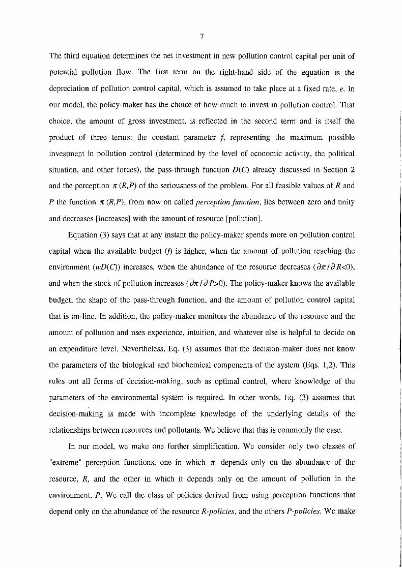
The third equation determines the net investment in new pollution control capital per unit of

potential pollution flow. The first term on the right-hand side of the equation is the

depreciation of pollution control capital, which is assumed to take place at a fixed rate, e. In

our model, the policy-maker has the choice of how much to invest in pollution control. That

choice, the amount of gross investment, is reflected in the second term and is itself the

product of three terms: the constant parameter f, representing the maximum possible

investment in pollution control (determined by the level of economic activity, the political

situation, and other forces), the pass-through function D(C) already discussed in Section 2

and the perception n (R,P) of the seriousness of the problem. For all feasible values of R and

P the function n (R,P), from now on called perception function, lies between zero and unity

and decreases [increases] with the amount of resource [pollution].

Equation (3) says that at any instant the policy-maker spends more on pollution control

capital when the available budget (f) is higher, when the amount of pollution reaching the

environment (wD(C)) increases, when the abundance of the resource decreases ( d n l d ReO),

and when the stock of pollution increases (dn I d P>O). The policy-maker knows the available

budget, the shape of the pass-through function, and the amount of pollution control capital

that is on-line. In addition, the policy-maker monitors the abundance of the resource and the

amount of pollution and uses experience, intuition, and whatever else is helpful to decide on

an expenditure level. Nevertheless, Eq. (3) assumes that the decision-maker does not know

the parameters of the biological and biochemical components of the system (Eqs. 1,2). This

rules out all forms of decision-making, such as optimal control, where knowledge of the

parameters of the environmental system is required. In other words, Eq. (3) assumes that

decision-making is made with incomplete knowledge of the underlying details of the

relationships between resources and pollutants. We believe that this is commonly the case.

In our model, we make one further simplification. We consider only two classes of

"extreme" perception functions, one in which n depends only on the abundance of the

resource, R, and the other in which it depends only on the amount of pollution in the

environment, P . We call the class of policies derived from using perception functions that

depend only on the abundance of the resource R-policies, and the others P-policies. We make

this distinction between R-policies and P-policies for two reasons. First, it is relevant for the

policy formulation process. Decision-makers need to know the pros and cons of waiting until

there is observed degradation of the resource to act as opposed to acting upon the evidence of

pollution, possibly even before degradation appears. Second, as we show below, the two

classes of policies can result in quite different consequences.

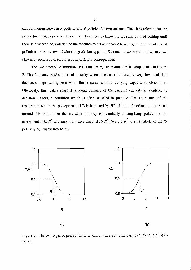
The two perception functions z (R) and z (P) are assumed to be shaped like in Figure

2. The first one, z (R), is equal to unity when resource abundance is very low, and then

decreases, approaching zero when the resource is at its carrying capacity or close to it.

Obviously, this makes sense if a rough estimate of the carrying capacity is available to

decision makers, a condition which is often satisfied in practice. The abundance of the

resource at which the perception is 112 is indicated by R*. If the p function is quite sharp

around this point, then the investment policy is essentially a bang-bang policy, i.e. no *

investment if R>R* and maximum investment if R<R*. We use R as an attribute of the R-

policy in our discussion below.

Figure 2. The two types of perception functions considered in the paper: (a) R-policy; (b) P-

policy.

Similarly, the perception function n (P) increases with pollution and is equal to zero

when P is low and equal to one when P is high. Of course "low" and "high" here means low

and high with respect to the values of pollution for which some impact on the resource is

detectable. Thus, perception functions of this kind make sense only when the influence of

pollution is at least roughly known.

3. ENVIRONMENTAL DYNAMICS WITH CONSTANT POLLUTION

CONTROL CAPITAL

In this section, we consider the dynamics of the model in the simple case where the

pollution control capital is constant. Before we begin, it is important to stress that the model

in Eqs. (1) and (2) is a very crude representation of the growth of a natural resource. The list

of phenomena which are not taken into account by these equations would be desperately long.

Indeed, the number of equations used to simulate the growth and decay of resources like

forests, crop production systems, and fisheries usually falls in the range from ten to one

hundred. On the other hand, even the addition of a single extra equation would give rise to an

analytically untractable problem. The low dimension of the model is therefore dictated by the

ultimate aim of the study, namely the formal derivation of general principles on

resource/pollution/policy interactions.

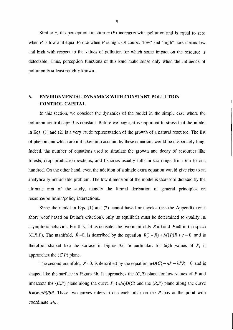
Since the model in Eqs. (1) and (2) cannot have limit cycles (see the Appendix for a

short proof based on Dulac's criterion), only its equilibria must be determined to qualify its

asymptotic behavior. For this, let us consider the two manifolds R =O and P =O in the space

(C,R,P). The manifold, R =0, is described by the equation R(l- R) + M(P)R + s = 0 and is

therefore shaped like the surface in Figure 3a. In particular, for high values of P , it

approaches the (C,P) plane.

The second manifold, P =0, is described by the equation wD(C) - aP - bPR = 0 and is

shaped like the surface in Figure 3b. It approaches the (C,R) plane for low values of P and

intersects the (C,P) plane along the curve P=(wla)D(C) and the (R,P) plane along the curve

R=(w-aP)lbP. These two curves intersect one each other on the P-axis at the point with

coordinate wla.

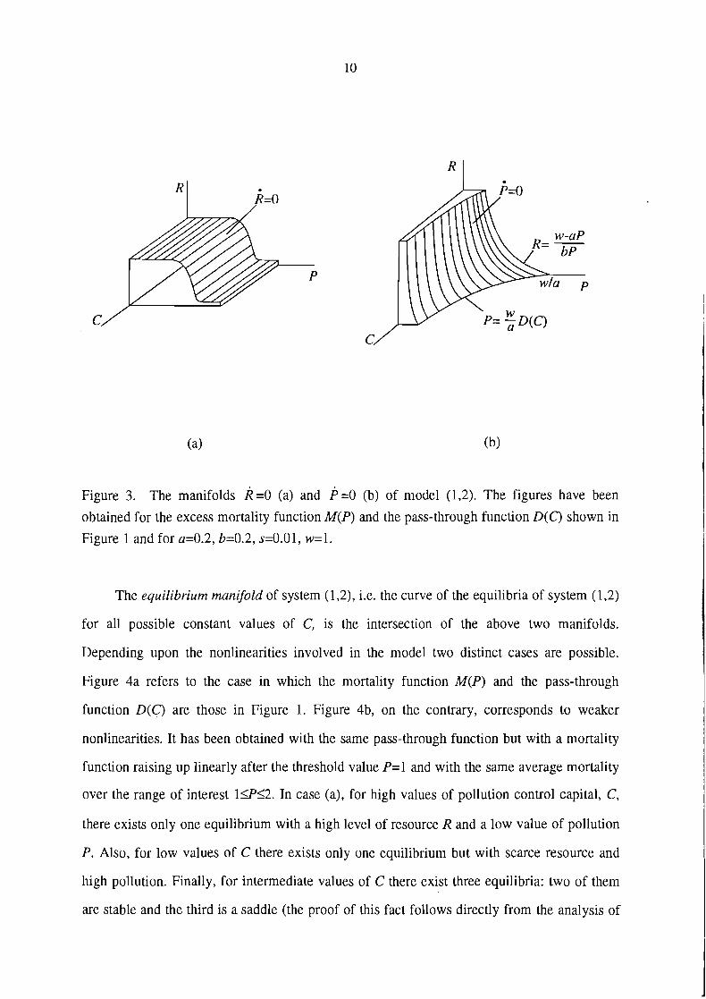
Figure 3. The manifolds R =O (a) and P =O (b) of model (1,2). The figures have been

obtained for the excess mortality function M(P) and the pass-through function D(C) shown in

Figure 1 and for a=0.2, b=0.2, s=0.01, w=l.

The equilibrium manifold of system (1,2), i.e. the curve of the equilibria of system (1,2)

for all possible constant values of C, is the intersection of the above two manifolds.

Depending upon the nonlinearities involved in the model two distinct cases are possible.

Figure 4a refers to the case in which the mortality function M(P) and the pass-through

function D(C) are those in Figure 1. Figure 4b, on the contrary, corresponds to weaker

nonlinearities. It has been obtained with the same pass-through function but with a mortality

function raising up linearly after the threshold value P=l and with the same average mortality

over the range of interest 1 9 1 2 . In case (a), for high values of pollution control capital, C,

there exists only one equilibrium with a high level of resource R and a low value of pollution

P. Also, for low values of C there exists only one equilibrium but with scarce resource and

high pollution. Finally, for intermediate values of C there exist three equilibria: two of them

are stable and the third is a saddle (the proof of this fact follows directly from the analysis of

the Jacobian of system (1,2)). Trajectories tend toward one or the other of the stable equilibria

depending upon their initial conditions. On the contrary, in case (b), multiple equilibria are

not present: for each value of C the system has only one equilibrium which is globally stable.

Figure 4. The equilibrium manifold of system (1,2) is the line obtained by intersecting the

manifolds R =O and P =O. Case (a) corresponds to the functions and parameters specified in

the caption of Figure 3. Case (b) corresponds to an excess mortality function which is linearly

increasing for P>1 and has the same average than the function shown in Figure l a in the

range 11P12.

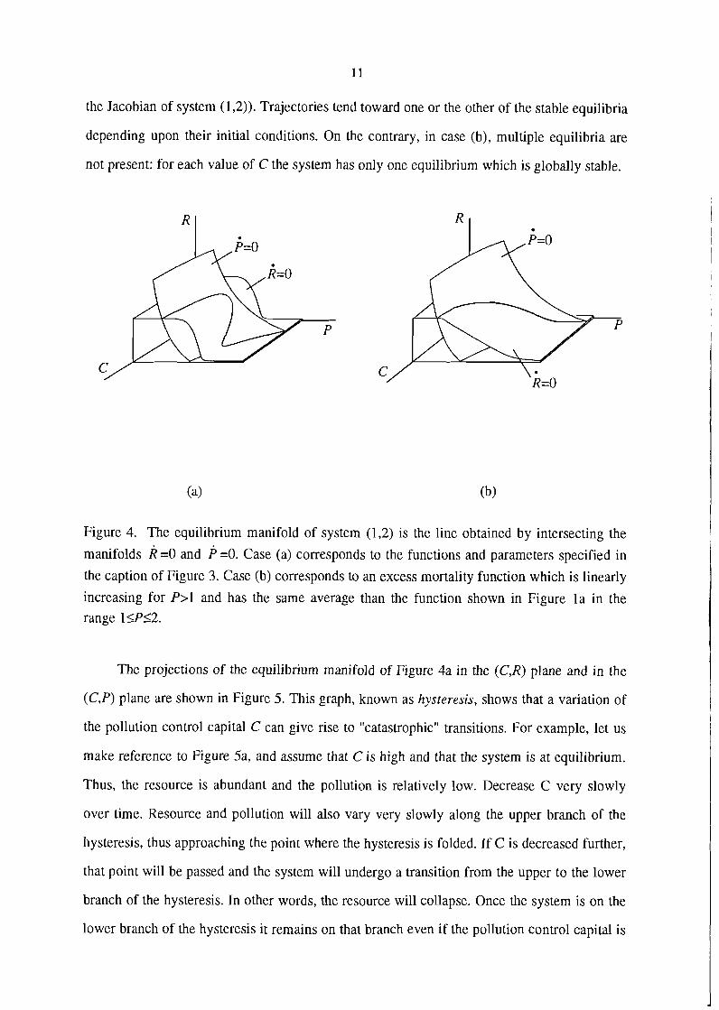
The projections of the equilibrium manifold of Figure 4a in the (C,R) plane and in the

(C,P) plane are shown in Figure 5. This graph, known as hysteresis, shows that a variation of

the pollution control capital C can give rise to "catastrophic" transitions. For example, let us

make reference to Figure 5a, and assume that C is high and that the system is at equilibrium.

Thus, the resource is abundant and the pollution is relatively low. Decrease C very slowly

over time. Resource and pollution will also vary very slowly along the upper branch of the

hysteresis, thus approaching the point where the hysteresis is folded. If C is decreased further,

that point will be passed and the system will undergo a transition from the upper to the lower

branch of the hysteresis. In other words, the resource will collapse. Once the system is on the

lower branch of the hysteresis it remains on that branch even if the pollution control capital is

slightly increased. The resource can be regenerated through a transition from the lower to the

upper branch of the hysteresis only if C is increased so much that the right fold is overcome.

Figure 5. The projection of the equilibrium manifold of Figure 4a on the (C,R) plane (a) and

on the (C,P) plane (b). These graphs illustrate hystereses. The upper and lower branches

(continuous lines) correspond to stable equilibria, while the dashed part corresponds to

unstable equilibria.

4. ENVIRONMENTAL DYNAMICS WITH VARIABLE POLLUTION

CONTROL CAPITAL

The dynamic behavior of system (1-3) will be analyzed assuming that C varies much

more slowly than R and P. This assumption is justified in a great number of cases, because of

the limited funds that are available for investment at any time and because there are often

important social and organizational constraints on how quickly new capital can be brought

into use. Technically speaking, this is the case if the two positive parameters e and f in Eq. (3)

are small. A relatively small e means that the pollution control capital does not depreciate

rapidly. A relatively small f means that the budget for pollution control capital is small so that

the pollution control capital can be increased only marginally in the short-run.

If C varies much more slowly than R and P, then the singular perturbation method

(Hoppensteadt, 1974) can be applied. This approach has been very often advocated and used

in ecology (see, for example, May, 1977; Ludwig et al., 1978; Berryman and Stenseth, 1984;

Holling, 1986; Rinaldi and Muratori, 1992a, 1992b) to point out the consequences of the

interactions between very small (or fast) and very big (01- slow) components of complex

ecosystems. Such a method says that the time evolution of the system is well approximated by

the concatenation of alternate fast and slow transients. In the present case, the fast transients

are time evolutions of R and P obeying Eqs. (1,2) with constant C. Such fast transients could

therefore be visualized in the three dimensional space (C,R,P) as trajectories developing in a

plane where C is constant and tending toward a stable equilibrium point of the fast system,

namely toward a point of the curve R = P = 0 shown in Figure 4. Once the state of the system

is on this curve it will move along it very slowly obeying Eq. (3). Of course the direction in

which the system moves is dictated by the sign of C. For this reason it is very useful to

visualize the manifold c=O which divides the state space into two regions: one in which the

slow motion is characterized by increasing values of C and the other where C decreases. Such

manifold is shown in Figure 6 for the two perception functions of Figure 2. Notice that this

manifold does not depend upon e and f separately, but only upon their ratio f/e.

If the fast system has no multiple equilibria (see Figure 4b), the slow transient ends at

an equilibrium point, as explicitly shown in Figure 7. On the contrary, when the fast system

has multiple equilibria (see Figure 4a) different scenarios are possible. Some of them involve

the collapse and/or the regeneration of the resource or even a slow-fast limit cycle, i.e. an

infinite sequence of concatenated slow and fast transients, where the fast ones are

alternatively associated with the collapse and the regeneration of the resource. We present

first the results for R-policies followed by those for P-policies.

Figure 6. The equilibrium manifold C=O of the slow subsystem (Eq. (3)) for the pass-

through function of Figure l b and f l e = 5 and for the two perception functions shown in

Figure 2: (a) R-policy; (b) P-policy.

Figure 7. The equilibrium manifold R = P =O of the fast subsystem (1,2) and the equilibrium

manifold c=O of the slow subsystem (3). The state of the system moves very slowly along

the manifold R = P =O and tends toward an equilibrium. The figure corresponds to the case of

no hysteresis shown in Figure 4b: (a) R-policy (see Figure 6a); (b) P-policy (see Figure 6b).

4.1. R-Policies

When the perception function depends only upon the abundance of the resource, the

manifold C=O is sloping downward in the space (C,R). In other words, the function R(C)

defined by Eq. (3) with c=O is decreasing. This is obviously true in general, since this

manifold gives the pollution control capital C that one should expect at equilibrium if the

resource R could be kept constant. A formal proof of this property can be given by letting

R=R(C) in Eq. (3) with c =O and then taking the derivative with respect to C, i.e.

which implies dRldC<O since dDldC<O and dpidR<O. Figure 8 shows three typical scenarios

corresponding to three different values of the ratio f ie . In case (a) the manifold C=O (dotted

line) intersects the equilibrium manifold R = P = 0 of the fast system at point (El) on the

upper branch of the hysteresis. Thus, all trajectories, (two of which, starting from points 1

and 2, are indicated in the figure) tend to this equilibrium. Notice, however that some of these

trajectories, like that starting from point 2, involve the collapse of the resource (vertical fast

trajectory going from point 2 to the C axis) and the regeneration of the resource (vertical fast

trajectory going from point C to point D). In case (b) the manifold c=O separates the two

branches of the hysteresis, so that a slow-fast limit cycle ABCD exists. Moreover, all

trajectories (like those starting from points 1 and 2) tend toward this cycle, which is therefore

globally stable. (The interested reader can refer to Muratori and Rinaldi (1991) for details on

the separation principle). In such a case the resource is in general either quite abundant or

almost absent and the periods of abundance and scarcity are very long, in comparison with

the periods of collapse (vertical fast trajectory AB) and regeneration (vertical fast trajectory

CD). Finally, in the third case the manifold c=O intersects only the lower branch of the

hysteresis, so that all trajectories tend toward a stable equilibrium E2 characterized by

extreme scarcity of the resource.

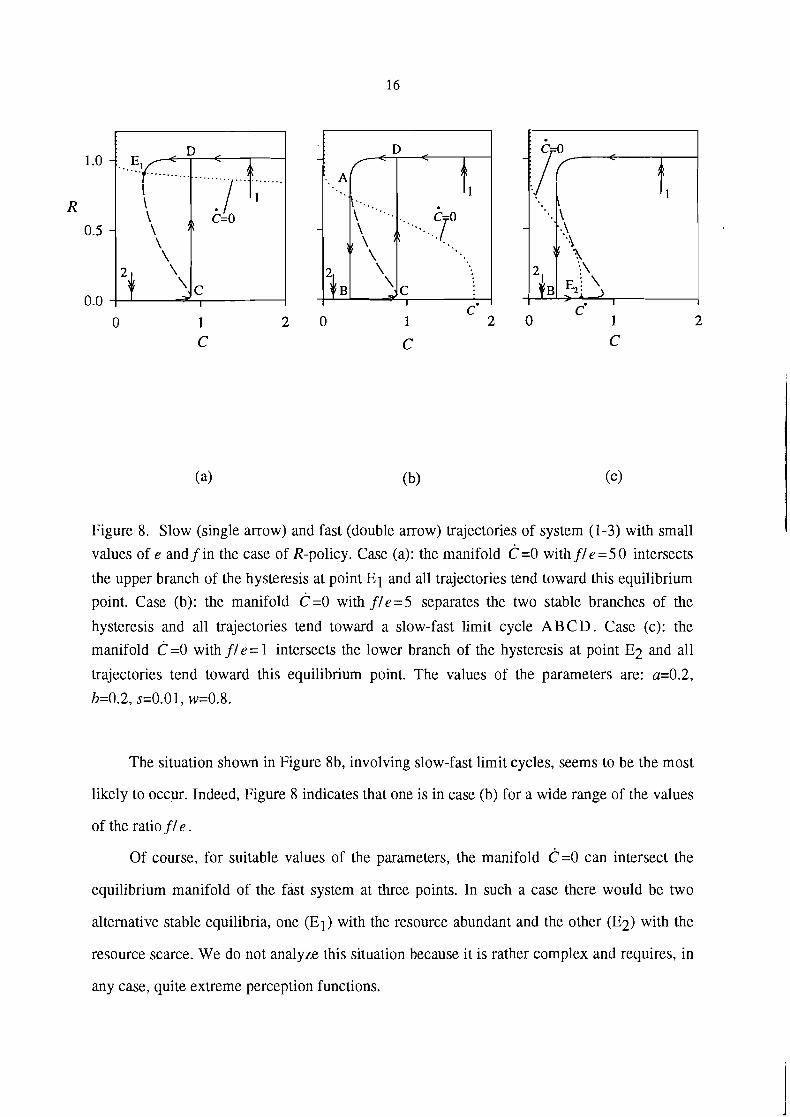
Figure 8. Slow (single arrow) and fast (double arrow) trajectories of system (1-3) with small

values of e and f in the case of R-policy. Case (a): the manifold c=O with f l e = 5 0 intersects

the upper branch of the hysteresis at point E l and all trajectories tend toward this equilibrium

point. Case (b): the manifold C=O with f l e = 5 separates the two stable branches of the

hysteresis and all trajectories tend toward a slow-fast limit cycle A B C D . Case (c): the

manifold c=O with f l e = 1 intersects the lower branch of the hysteresis at point E2 and all

trajectories tend toward this equilibrium point. The values of the parameters are: a=0.2,

b=0.2, s=0.01, w=0.8.

The situation shown in Figure 8b, involving slow-fast limit cycles, seems to be the most

likely to occur. Indeed, Figure 8 indicates that one is in case (b) for a wide range of the values

of the ratio fl e .

Of course, for suitable values of the parameters, the manifold c=O can intersect the

equilibrium manifold of the fast system at three points. In such a case there would be two

alternative stable equilibria, one (El) with the resource abundant and the other (E2) with the

resource scarce. We do not analyze this situation because it is rather complex and requires, in

any case, quite extreme perception functions.

4.2 . P-Policies

When the perception function depends upon pollution like in Figure 2b the main

scenarios are like those shown in Figure 9. Two of them (Figures 9a and 9c) are characterized

by a unique stable equilibrium point. This equilibrium can have either a low pollution level

(and consequently with the resource abundant) as point El (Figure 9a) or a high pollution

level (and hence a very scarce resource) as point E2 (Figure 9c). On the contrary, the

intermediate scenario is characterized by the existence of two alternative stable equilibria E l

and E2. Thus, the collapse of the resource cannot be endogenously generated: it can only be

the consequence of a severe pollution accident or of an unexpected failure of the treatment

facilities, bringing the state of the system from the equilibrium E l into the basin of attraction

of the alternative equilibrium E2.

Figure 9. Slow (single arrow) and fast (double arrow) trajectories of system (1-3) with small

values of e and f in the case of P-policy (see Figure 2b). Case (a): the manifold c=O with

f /e=5 intersects the lower branch of the hysteresis at point E l and all trajectories tend toward

this equilibrium point. Case (b): the manifold C=O with f/e=2.5 intersects both stable

branches of the hysteresis at points E l and E2 and some trajectories tend toward E l while

others tend toward E2. Case (c): the manifold C=O with f /e= 1 intersects the upper branch of

the hysteresis and all trajectories tend toward this equilibrium point. The values of the

parameters are a=0.2, b=0.2, s=0.01, w=l.

18

Mathematically speaking, the case in which the manifold c=O separates the two stable

branches of the hysteresis (and therefore in which slow-fast limit cycles exist) is also

possible. Nevertheless, this situation, requires the use of a sharp perception function, a low

depreciation (e), in comparison with maximum investment rate 0, and a level P* (see Figure

2b) very close to the pollution level at which the resource cannot grow (because the upper

branch of the hysteresis shown in Figure 9 corresponds to virtual extinction of the resource).

For all these reasons it is very unlikely that the resource would collapse if P-policies are used.

Nevertheless, P-policies can be very unpopular because they might require a consistent

economic effort before any sign of deterioration of the resource is detectable. On the

contrary, R-policies are more popular but the previous analysis has shown that a poor

understanding of the behavior of the system, giving rise to a poor design of the pollution

control actions, can be quite dangerous if R-policies are used.

5. INFLUENCE OF ECONOMY AND OF POLLUTION CONTROL POLICY

In this section, we consider the influence of the economy and of the pollution control

policy on the dynamic behavior of system (1-3).

Assuming that the system is at equilibrium with an abundant resource and low pollution

and that the decision-maker uses R-policies, an increase in the potential pollution flow w,

such as might arise from an increase in population size or an increase in economic activity per

person, could trigger a transition to a cyclic regime. A qualitative proof is the following (see

Figure 8a). The graph C=O in the (C,R) plane is not influenced by w, because w does not

appear in Eq. (3). On the other hand, given an equilibrium (R,P) of system (1,2) where C is

considered as a parameter, if w increases, then, from Eq. (2) with P =0, it follows that wD(C)

must remain constant, i.e. C (see Figure lb) must increase. This means that the hysteresis,

shown in Figure 8a, shifts to the right. Thus, if w increases sufficiently, the graph c=O will

separate the two stable branches of the hysteresis and a slow-fast limit cycle will appear.

Consequently, increasing w from a value corresponding to an equilibrium for system (1-3) to

a value corresponding to a slow-fast limit cycle, implies first the collapse of the resource,

then a long period of scarce resource and, finally, the regeneration initiating the slow-fast

cycle.

Sudden collapses of the resource may also occur even if the increase in w does not

produce slow-fast cycles. For example Figure 10 shows the case in which a 20% increase of

w gives rise to the collapse of the resource followed by a long period of scarcity before

regeneration finally takes place.

C time

Figure 10. Collapse and regeneration of the resource due to an increase of the potential

pollution flow w. The two hystereses shown in (a) correspond to two different values of the

potential pollution flow, w=0.8 and w1=0.96, while the manifold C=O corresponds to f l e=5 .

If e and f are small and the potential pollution flow is increased from w to w', the system tends toward the new equilibrium I$ through a sequence of fast and slow transients

E 1 B ' C 'D ' &. The time pattern of the resource for e=0.0 1 and fi0.05 is shown in (b) where t

is the time at which the potential pollution flow is increased and t' is the time at which the

resource is regenerated (see point D' in (a)).

The influence of w on the slow-fast limit cycle is also quite easy to detect. As already

said, when w is increased, the hysteresis shifts to the right and its lower branch becomes

closer and closer to the manifold C=O. This means that c becomes smaller and smaller on

this branch and this implies that the period of time separating collapses and regenerations

increases with w. Figure 11 confirms this analysis showing the limit cycles corresponding to

three different values of w and to small values of e and$

We now consider the effects of two parameters of an R-policy, namely R* (the amount

of resource at which the perception n: (R) is 112) and f (the maximum investment rate). The

analogous discussion for P-policy is left to the reader.

0 200 400 600 800 1000

time

Figure 11. In a cyclical regime, the period during which the resource is scarce increases with

the potential pollution flow (w=l; 1.16; 1.18 from top to bottom). The figure has been

produced using the functions of Figure 1, the R-policy of Figure 2a and the parameter values

a=0.2, b=0.2, s=0.01, e=0.01,&0.05.

The influence of R* on system (1-3) can be easily seen in the case of an extremely

sharp perception function s (R). In fact, in such a case, if R* decreases, the manifold C=O in

Figure 8a will shift downward and will therefore eventually separate the two stable branches

of the hysteresis, thus giving rise to a cyclic regime. The (obvious) conclusion is that low R*

values are dangerous.

The influence off on system (1-3) can also be predicted by looking at its influence on

the manifold c =O. For fixed R, an increase of f implies an increase of C (see Eq. (3) with

c =O), i.e. the manifold c =O shifts to the right. Therefore, lowering f, can cause a transition

from a stationary to a cyclic regime. In other words, too low a value of the budget can also be

dangerous.

If the number of people increases, we would expect that both w and f would increase

(other things equal, a larger population would pollute more, but would also have the resources

to invest more in pollution control). Figure 12a (obtained through simulation) shows the

influence of w and f on system (1-3). To the left of the curve, the system is stationary; to the

right, it is cyclic. Imagine a system characterized by w=0.5 andfi0. l . In this case, the system

will go to an equilibrium. Now if the number of people doubles, so that w=1.0 and@O.2, the

system will exhibit cycles wit11 collapses and regenerations of the resource. Thus, an increase

of population size can cause an abrupt transition from stationary to cyclic behavior.

In order to mitigate the negative effects induced by a reduction off, one can increase s

by stocking, if this is feasible. In fact an increase of s (see Eqs. (1,2) with R =O and P =0)

shifts the hysteresis of Figure 8a to the left while a reduction off shifts it to the right. Figure

12b confirms this possibility, by representing the curve in the plane (f,s) (obtained through

simulation) that separates the stationary and cyclic regimes.

cyclic

I I I

Figure 12. The regions of stationary and cyclic regimes in parameter space. The curves

separating the two regions have been obtained through simulation, using the functions of

Figure 1, the R-policy of Figure 2a and the parameter values u=0.2, b=0.2, e=0.01. Moreover,

in (a) s=0.01, while in (b) w=0.63.

6. CONCLUSIONS

In this paper, we introduce a simple third order model of the interactions between

resource abundance (R), pollution (P), and pollution control capital (C) and show that its

behavior can be analyzed graphically using the singular perturbation approach. The model

produces two types of behavior, stationary and cyclic. In the latter case, the resource goes

through periods of growth and collapse punctuated by long periods of abundance or scarcity.

We distinguish between two classes of environmental policies, one in which decision-makers

base investments in pollution control on the abundance of the resource, R-policies, and

another in which they base their decisions on the amount of pollution they observe, P-

policies. We show that it is safer for decision-makers to focus on pollution rather than on the

abundance of the resource because under R-policies small changes in one element of the

policy mix can cause a discontinuous change from a high resource equilibrium to a cycle that

begins with an almost total collapse of the resource. Increases in population, economic

activity, or technological changes can also cause such a discontinuous change, even when

they are accompanied by a proportional increase in the amount of funds available for

pollution control. On the contrary, when P-policies are used, the system is much more

difficult to crash.

Our analysis can be expanded in a number of directions. For example, if the dynamics

of the resource depends upon the pollution flow (wD(C) in Eq. (2)), like in the case of trees

with leaves damaged by acidic precipitation, the same model can be used, provided the

dependence of the excess mortality of the resource upon the pollution flow is specified. This

corresponds to an assumption that M in Eq. (1) is a suitable function of wD(C). Then, the

same geometric approach used in this paper can be followed, assuming again that the

pollution control capital varies much more slowly than R and P. Another interesting extension

would be to consider more sophisticated decision support systems. For example, one could

assume that information on both R and P is available to the decision maker who, then, call use

(R,P)-policies (instead of R-policies or P-policies) to decide how much to invest in pollution

control. Again, our geometric approach could be used to analyze the consequences of any

specified (R,P)-policy. But the same approach can also be used to solve an interesting inverse

problem, namely the determination of a (R,P)-policy which is at the same time safe (as the P -

policies) and popular (as the R-policies). Finally, one could also try to extend the present

study by modeling in a more accurate way one (or more) of the compartments of the system.

For example, one could study the case in which the resource is the top component of a three

level food chain, thus using three differential equations to describe the dynamics of R. Letting

the rest unchanged, the resulting system would be of order 5. The singular perturbation

approach could still be applied to it, under the assumption that P and the three components of

the food chain vary more quickly than C. Nevertheless, the analysis would certainly be less

transparent, because the high dimensionality of the model would destroy the possibility of

showing the results by means of simple graphs, as done in this paper.

APPENDIX

This Appendix shows that model (1,2) with constant C cannot have strictly positive

limit cycles. The proof is a simple application of Dulac's criterion for non-existence of limit

cycles. Such a criterion says the following (Strogatz, 1994): "Let x = F(x ) be a continuously

differentiable vectorfield defined on a simply connected subset S of the plane. If there exists a

continuously differentiable, real-valuedfinction g(x) such that the divergence of g(x)F(x) has

one sign throughout S, then there are no closed orbits lying entirely in S."

In our case the function g exists since

gives

so that

which is strictly negative inside the positive quadrant. Therefore, no strictly positive limit

cycle exists.

REFERENCES

Benyman, A.A. and N.C. Stenseth. 1984. Behavioral catastrophies in biological systems. Behavioral

Science 29: 127-137.

Clark, C.W. 1990. Mathematical Bioeconomics: The Optimal Management of Renewable Resources.

New York, USA: John Wiley & Sons.

Fisher, A.C., W.M. Hanemann, and A.G. Keeler. 1991. Integrating fishery and water use

management: A biological model of a California salmon fishery. Journal of Environmental

Economics and Management 20:234-26 1.

Gatto, M. and S. Rinaldi. 1987. Some models of catastrophic behavior in exploited forests. Vegetatio

69~213-222.

Holling, C.S. 1986. The resilience of terrestrial ecosystems: Local surprise and global change. Pages

292-317 in W.C. Clark and R.E. Munn, eds. Sustainable Development of the Biosphere.

Cambridge, UK: Cambridge University Press.

Hoppensteadt, F. 1974. Asymptotic stability in singular perturbation problems. Journal of Differential

Equations 155 10-521.

International Institute for Applied Systems Analysis. 1993. Acidification: Modeling transboundary air

pollution. Options. Winter. Laxenburg, Austria.

Kishi, M., J.M. Uchiyama, and Y. Iwata. 1994. Numerical simulation model for quantitative

management of aquaculture. Ecological Modelling 72:21-40.

Ludwig, D., D.D. Jones, and C.S. Holling. 1978. Qualitative analysis of insect outbreak systems: The

spruce budworm and forest. Journal of Animal Ecology 47:315-332.

May, R.M. 1977. Thresholds and breakpoints in ecosystems with a multiplicity of stable states.

Nature 269:471-477.

Muratori, S. and S. Rinaldi. 1991. A separation condition for the existence of limit-cycles in slow-fast

systems. Applied Mathematical Modelling 15:3 12-3 18.

Noy-Meir, I. 1975. Stability of grazing systems: An application of predator-prey graphs. Journal of

Ecology 63:459-483.

Rinaldi, S., R. Soncini-Sessa, H. Stehfest, and H. Tamura. 1979. Modeling and Control of River

Quality. London, UK: McGraw Hill.

Rinaldi, S. and S. Muratori. 1992a. Limit cycles in slow-fast forest-pest models. Theoretical

Population Biology 41 :26-43.

Rinaldi, S. and S. Muratori. 1992b. Slow-fast limit cycles in predator-prey models. Ecological

Modelling 6 1 :287-308.

Strogatz, S.H. 1994. No~zlinear Dynamics and Chaos. Reading, MA: Addison-Wesley.

United Nations Economic Commission for Europe. 1994. Protocol to the 1979 convention on long-

range transboundary air pollution on further reduction of sulphur emissions. Geneva,

Switzerland.

Walters, C. 1986. Adaptive Management of Renewable Resources. New York, USA: Macmillan.