Embed Size (px)
Citation preview

15 February 2019
POLITECNICO DI TORINORepository ISTITUZIONALE
2-D and 3-D tools for electrical imaging in environmental applications / Arato, Alessandro. - (2013).Original
2-D and 3-D tools for electrical imaging in environmental applications
Publisher:
PublishedDOI:10.6092/polito/porto/2510297
Terms of use:openAccess
Publisher copyright
(Article begins on next page)
This article is made available under terms and conditions as specified in the corresponding bibliographic description inthe repository
Availability:This version is available at: 11583/2510297 since:
Politecnico di Torino

POLITECNICO DI TORINO
Dottorato in Ambiente e Territorio
Georisorse e Geotecnologie
XXV Ciclo
TESI DI DOTTORATO
“2-D and 3-D tools for electrical imaging
in environmental applications”
Tutore: Candidato:
Prof. ALBERTO GODIO Ing. Alessandro Arato
Aprile 2013

Acknowledgements
After these three years of PhD experience, there is a certain number of people I would like to thank.
Foremost, my gratitude goes to my advisor, Prof. Alberto Godio, for having shared his knowledge
with me during these three years with patience, motivation and stimulating discussions. He accepted
my application to the PhD program here at Politecnico di Torino, indirectly opening a very special
period with all the fellows of the group of Applied Geophysics (and the department in general).
I would also to thank some important people, with whom I worked on most of the material
presented in this thesis. In order of “appearance”: Prof. Luigi Sambuelli, Dr. Andrea Borsic, Dr.
Alberto Villa, Dr. Markus Wehrer and Prof. Borbala Biró. You will sometimes read, scrolling
throughout the thesis, some sentences starting with “We tested...”, “We performed...”, “We have
applied...”. I intentionally decided to leave the plural form because I cannot attribute all the thoughts
and work to myself and, in fact, most of the work presented in this thesis will be published in
different forms with their co‐authorship.
Of course, I can’t omit the beautiful experience with all SoilCAM people I met during these years at
meetings, conferences, and field activities. We shared poster sessions and focus groups, rain and sun,
mud and oil, pizza and wine.
A huge GRAZIE goes to my colleagues, starting from Diego and all the field work we have done
together (and, of course, all lunches at Bella Riva, some curious discussions with truckers at le due
pazze and some polenta on the alpine glaciers), and going to Paolo, Flora, Roberto Bruno, Stefano,
Daniele, Margherita, Corrado, Ema, Ken, Silvia, Erika, Sylvester, Federico, Prof. Valentina Socco and
Dr. On. Cesare Comina. We shared an innumerable quantity of coffees and pauses, soccer matches,
bottles of good and “aged” wine, a lot of laughs and, why not?, important advices on Matlab tools
that were completely unknown to me.
The final part of the acknowledgements is for the most important people. ALL OF MY FRIENDS, my
family and Roberta, who I literally share my life with. Their daily support is unconditional and selfless,
and their love is the most important thing for me.

Summary
Introduction 1
Description of Trecate site 2
Organization of the thesis 3
References 5
1. Theoretical Background 7
1.1 Physical Principles 7
1.2 Petrophysical interpretation of geo‐electrical parameters 8
1.2.1 Electrolytic conductivity 9
1.2.2 Surface conductivity and membrane polarization 9
1.2.3 Electronic conductivity 11
1.3 Field measurements and related geophysical parameters 12
1.3.1 IP measurements in time‐domain 12
1.3.2 IP measurements in frequency domain 13
1.4 Inversion of electrical resistivity data 14
1.4.1 2‐D inversion 17
1.4.2 3‐D inversion 18
1.5 Use of a‐priori information in electrical resistivity problems 19
1.6 Application of Electrical Resistivity and Induced Polarization methods for contamination
mapping and (bio‐)degradation assessment 22
1.6.1 Hydrocarbon contamination of sedimentary soils 23
References 24
2. Staggered grid inversion of cross hole resistivity tomography 29
2.1 Introduction 29
2.2 The Staggered Grid method applied to 2‐D Electrical Resistivity Tomography 30
2.2.1 Application to synthetic data 32
Synthetic model n. 1 33
Synthetic model n. 2 34
2.2.2 Application to real data 36
2.3 Results and discussion 38

2.3.1 Synthetic model n.1 38
2.3.2 Synthetic model n.2 39
2.3.3 Field dataset 42
2.4 Conclusions 45
References 46
3. Forward modeling and inversion for 2‐D and 3‐D real/complex electrical resistivity data 48
3.1 Mesh Generation 49
3.2 Inversion of complex resistivity datasets 52
3.3 Application to synthetic data 54
3.4 Application to real cases 57
3.5 Discussion and conclusions 63
References 65
4. Time‐lapse inversion of electrical resistivity data 69
4.1 Application of SGERT to time‐lapse Electrical Resistivity Tomography 71
4.2 Joint use of staggered grid and difference inversion 73
4.3 Application to synthetic data 74
4.4 Application to real data 83
4.5 Conclusions 88
References 90
5. Integration of geophysical and geochemical data for the characterisation of biological
degradation at an aged LNAPL‐contaminated site 91
5.1. Material and methods 92
5.1.1 Geophysical characterization 92
5.1.2 Monitoring of chemico‐physical parameters in soil and groundwater samples 92
5.1.3 Microbial counts of bacteria in below‐ground soil layers in Trecate 93
5.2 Results and discussion 95
5.2.1 Borehole 1‐D profiling 95
5.2.2 2‐D complex resistivity tomography 98
5.2.3 Distribution of chemico‐physical parameters 100
5.2.4 Microbial Counts 104

5.3 Conclusions 106
References 107
CONCLUSIONS 108

1
Introduction
This work is focused on the characterization of sedimentary soils affected by contamination, and
on the monitoring of the evolution of contaminant distribution and properties over space and
time. Within this initial purpose, geo‐electrical and electromagnetic techniques have been used
and analysed. More specifically, bi‐dimensional (2‐D), tri‐dimensional (3‐D) and time‐lapse (4‐D)
geo‐electrical methods make up the core of the work presented in this thesis.
The traditional electrical resistivity measurements originate in the 1910s, with the famous works
on resistivity soundings by Schlumberger and Wenner. Since then, use of geoelectrical methods
have increased, due to their effectiveness in providing useful information about subsoil in many
different applications (e.g. mineral exploration, hydrogeological characterization at shallow
depth).
Tomographic methods (i.e. Electrical Resistivity Tomography, ERT) hugely came up since the early
1980s (e.g. Barker, 1981) when proper instrumental devices and computing facilities were
developed, allowing geophysicists to perform 2‐D electrical resistivity surveys with reasonable
effort, in terms of both time consumption and computation costs. The possibility to get more
detailed information, and the further development of cross‐hole methods, made ERT a desirable
technique even for environmental applications. Hydrogeophysical studies have been conducted to
monitor flow and transport of water and contaminants in the vadose zone (e.g. Cassiani et al.,
2006), in aquifers and fractured rocks (e.g. Daily et al., 1992, Binley et al., 1996, Slater et al., 1996,
1997), to delineate contaminant plumes (e.g. Daily et al., 1995), and to follow the evolution of
remediation processes in contaminated sites (e.g. Ramirez et al., 1993, LaBrecque et al., 1996c).
The joint use of electrical resistivity and Induced Polarization (IP) methods have been used in a
variety of situations concerning contaminated cases (e.g. Mazác et al., 1990; Benson and Stubben,
1995; Grumman and Daniels, 1995; Atekwana et al., 2000), exploiting the possibility to detect
contaminant as well‐recognisable geophysical anomalies. In fact, the principal phenomena which
underlie the physical phenomena of electrical conduction and polarization in soils are well known
at present. Inversion algorithms for the inversion of complex resistivity data have been developed
(e.g. Kemna, 2000, De Bacco, 2003) in the last decade, allowing to incorporate both the real and
imaginary components of the resistivity, respectively related to conduction and to polarization
phenomena in the investigated medium.

INTRODUCTION
2
However, the need to improve the resolution of resistivity imaging technique without stressing
the intrinsic under‐determination of the geo‐electrical problem, and to provide more robust
results in integrated characterization approaches, guided the work presented in this thesis to
works on both “static” 2‐D and 3‐D problems, and on the inversion of time‐lapse data. In addition,
joint characterization of contaminated site has been carried out together with chemico‐physical
and biological analysis.
Grid manipulation techniques have been explored and adapted to the inversion of geo‐electrical
data, in order to solve inversion of resistivity data set trying to improve space resolution without
decaying the robustness of the inversion process. Furthermore, in order to provide a
mathematically flexible algorithm for inversion of complex resistivity data, a software based on
the Primal‐Dual method, through which the user can decide to use either the L1‐ or the L2‐ norm
on both the data and regularization term of the objective function, has been created and tested.
Strategies related to the inversion of electrical resistivity and IP data have been developed with
the aim of improving the interpretability of the results both in space and in time. These activity
are part of a common effort for achieving an integrated characterization of contaminated sites,
jointly with chemico‐physical analysis of soils and groundwater and with measures of presence
and degradation activity of hydrocarbon‐degrading biomass.
This thesis is aimed to provide a methodological approach to inversion of 2‐D and 3‐D electrical
resistivity data, in a variety of possible situations. However, most of the experimental activity
presented in the various chapters has been carried out on data coming from a hydrocarbon‐
contaminated site, within the framework of the EU FP7 SoilCAM project. The application to data
coming from a challenging test‐site strengthens the confidence in the techniques developed in
this thesis.
Description of Trecate site
The contaminated site treated in this thesis is located near the town of Trecate, in North‐West of
Italy. The Trecate area is characterised by fluvio‐glacial and fluvial deposits, made up of a thick
sequence of poorly sorted silty sands and gravel in extensive lenses. An artificial layer of clayey‐
silty material, less than 1 m thick, which was originally placed as a rice paddy liner, covers most of
the site.
The shallow aquifer at the Trecate site comprises an extensive, unconfined sand and gravel unit in
excess of 60 m thick beneath the site. The regional groundwater flow is influenced by the

INTRODUCTION
3
previously described local conditions, because of the recharge, which occurs through the water
infiltration from irrigation channels and rice‐paddies, and because of the horizontal outflow,
which is influenced by the drainage taken by the Ticino river, located in the Eastern direction 20 m
below the elevation of the surrounding areas.
In 1994, the site was subjected to a crude oil spill as a result of a well blow out from an ENI‐Agip
operated exploration well, designated Trecate 24 (TR24). Details of the incident, which resulted in
approximately 15,000 cubic meters of middleweight crude oil being released onto the surface and
which contaminated both the soil and groundwater, have been reported elsewhere, together with
descriptions of the subsequent site remediation (Reisinger et al., 1996, Brandt et al., 2002). After
the accident, most of the oil was quickly collected and disposed of, but some infiltrated into the
subsurface and reached the groundwater table. The oil mainly infiltrated where the clay liner was
weak or absent, particularly at some rice paddy infiltration pits. On‐site washing and thermal
treatment of the soil was performed to speed up the soil remediation.
A permanent monitoring network was installed for groundwater control. The temporal evolution
of the soil and the groundwater pollution has been assessed by conducting two field surveys per
year, using direct‐push technology to collect soil samples.
NAPL lenses have been detected floating on the water table since the blow‐out occurred. The
main hydrocarbon contamination zone covers approximately 96,000 m2 and is characterized by an
anoxic, electrochemically reductive groundwater plume (Burbery et al., 2004).
High contamination has been found both in soil samples (with TPH concentration values up to 500
mg/kg) and in the groundwater (TPH concentration > 10 mg/l).
Organization of the thesis
The first chapter gives an introduction about the geo‐electrical problems, both from a theoretical
and a practical point of view. It introduces the physical laws which govern the electrical and
electromagnetic phenomena discussed in the thesis, the possible interpretation of the results, the
measure of field parameters and the theory on inversion of electrical resistivity data.
In the second Chapter a novel approach, called Staggered Grid Electrical Resistivity Tomography,
is presented. It is based on the manipulation of Finite Element Model grids and it works in a
different way over homogeneous resistivity zones and across zones of high resistivity gradient.
Thus, the user can check for the reliability of the resulting resistivity image, and even detecting
more accurately the presence of resistivity boundaries.

INTRODUCTION
4
The third Chapter focuses on the development of a software for the inversion of 2‐D and 3‐D
complex resistivity data. The code, developed jointly with Dr. A. Borsic (Dartmouth College, New
Hampshire), is implemented on the Primal‐Dual Interior Point Method (PDIPM), which gives the
user a high mathematical flexibility and allows to reduce the sensitivity of the inversion process to
the presence of outliers in the data and to preserve sharp resistivity edges, where present.
Furthermore, adaptive Finite Element meshing with the possibility to model the electrodes with a
finite size allows a more rigorous solution of the direct problem.
An extension of the SGERT method is presented in the fourth Chapter, which deals with time‐
lapse inversion of resistivity data. Static SGERT technique is combined with the Difference
inversion method (LaBrecque and Yang, 2001) to improve the quality of time‐lapse results and to
give additional information on the reliability of time‐lapse results.
The fifth Chapter shows the results of a long‐term geo‐electrical, chemico‐physical and biological
monitoring at the hydrocarbon‐contaminated site of Trecate (NO, Italy). The geophysical 1‐D and
2‐D characterization is supported by direct measurements of the most important chemico‐
physical parameter of soil and groundwater samples, and by laboratory experiments to check the
presence of biomass and its degrading activity.

INTRODUCTION
5
References Atekwana, E. A., Sauck,W. A., Werkema, D. D., 2000. Investigations of geoelectrical signatures at a
hydrocarbon contaminated site. J. Appl. Geophys., 44, 167–180.
Barker, RD., 1981. The offset system of electrical resistivity sounding and its use with multicore
cable. Geophy. Prosp., 29, 128‐143.
Binley, A., Shaw, B. and Henry‐Poulter, S., 1996. Flow pathways in porous media: electrical
resistance tomography and dye staining image verification. Meas. Sci. Technol., 7, 384–390.
Benson, A. K., Stubben, M. A., 1995. Interval resistivities and very low frequency electromagnetic
induction—An aid to detecting groundwater contamination in space and time: A case study.
Environmental Geoscience, 2, 74–84.
Brandt, C.A., Becker, J.M., Porta, A., 2002. Distribution of polycyclic aromatic hydrocarbons in soils
and terrestrial biota after a spill of crude oil in Trecate, Italy. Environ. Toxicol. Chem., 21, 1638–
1643.
Burbery. L., Cassiani. G., Andreotti. G., Ricchiuto. T., Semple. K.T., 2004. Single‐well reactive tracer
test and stable isotope analysis for determination of microbial activity in a fast hydrocarbon‐
contaminated aquifer. Environ. Pollut., 129, 321–330.
Cassiani, G., Bruno, V., Villa, A., Fusi N., and Binley, A. M., 2006. A saline tracer test monitored via
time‐lapse surface electrical resistivity tomography. Journal of Applied Geophysics, 59, No. 3, 244‐
259.
Daily, W.D., Ramirez, A.L., LaBrecque, D.J., Nitao, J., 1992. Electrical resistivity tomography of
vadose water movement. Water Resources Research, 28, 1429‐1442.
Daily, W., Ramirez, A., LaBrecque, D., Barber W., 1995. Electrical resistance tomography
experiments at the Oregon Graduate Institute. Journal of Applied Geophysics, 33, 227‐237.
De Bacco, G., 2003. Tomografia di resistività complessa:soluzione del problema diretto e
inversoper applicazioni ingegneristiche egeologico‐ambientali. PhD thesis.
Grumman,D. L., Daniels, J. J., 1995. Experiments on the detection of organic contaminants in the
vadose zone. Journal of Environmental and Engineering Geophysics, 0, 31–38.
Kemna, A., 2000. Tomographic inversion of complex Resistivity. Theory and application. PhD
Thesis. Der Andere Verlag.
LaBrecque, D. J., Ramirez, A.L., Daily, W.D., Binley, A.M., Schima, S., 1996c. ERT monitoring of
environmental remediation processes. Meas. Sci. Tech., 7, 375‐383.

INTRODUCTION
6
La Brecque, D. J., Yang, X., 2001. Difference inversion of ERT data: a fast inversion method for 3‐D
in situ monitoring. Journal of Environmental and Engineering Geophysics, 6, 83–89.
Mazác, O., Benes, L., Landa, I., Maskova, A., 1990. Determination of the extent of oil
contamination in groundwater by geoelectrical methods. In Ward , S. H., Ed., Geotechnical and
environmental geophysics II: Society of Exploration, Geophysicists, 107–112.
Ramirez, A.L., Daily, W.D., LaBrecque, D.J., Owen, E., Chesnut, D.,1993. Monitoring an
underground steam injection process using electrical resistance tomography. Water Resources
Res., 29, 73‐87.
Reisinger, HJ., Mountain, SA., Andreotti, GD., Porta, A., Hullman, AS., Owens, V., Arlotti, D.,
Godfrey, J., 1996. Bioremediation of a major inland oil spill using a comprehensive integrated
approach. Proceedings of the 3rd International Symposium of Environmental Contamination in
Central and Eastern Europe Warsaw Florida State University.

7
1. Theoretical Background
1.1 Physical Principles
The theory behind electrical resistivity methods is based on the Maxwell’s Equations. They
provide a comprehensive description of the macroscopic electromagnetic behaviour of a medium.
The electric and magnetic fields are both described by their intensity, respectively:
t
B
E (1.1.a)
t
s
DH J J (1.1.b)
where E and H are, respectively, the electric and magnetic field intensity, B is the magnetic
induction, J the conduction current density, D the electric displacement and Js a general current
source into the medium.
Equations (1.1) are related each other and can be simplified under the assumption of a linear,
isotropic and time‐invariant medium, in frequency domain:
= σ( ) J E (1.2.a)
= ( ) D E (1.2.b)
B H (1.2.c)
where σ(ω) and ε(ω) are, respectively, the electric conductivity and the dielectric permittivity,
function of angular frequency ω, and μ the magnetic permeability.
The electromagnetic field which is generated by an alternating current through a medium can be
expressed as a function of the complex exponential tie , resulting in:

THEORETICAL BACKGROUND
8
i E H (1.3.a)
( ( ) i ( ) ) sH E J (1.3.b)
At low frequencies, when f=ω/2π < 10 kHz as in the case of electrical resistivity surveys, the
following condition is valid:
1
(1.1)(1.2)(1.3)(1.4)
Thus, electric conduction is the preponderant phenomenon and then the displacement current
term D (in Equation 1.2.b), which regulates the propagation of electromagnetic waves at high
frequency, can be neglected.
Conductivity σ, as the reciprocal of resistivity ρ, is then the physical property that governs current
flow through the ground, as described by the Ohm’s Law (Equation 1.2a).
Supposing E to be conservative, and in absence of magnetic perturbations, the electric field
intensity is given as the gradient of the electric potential,
E (1.5)
and the Ohm’s Law can be rewritten as:
( ( )) 0 sE J (1.6)
1.2 Petrophysical interpretation of geo‐electrical
parameters
This section is aimed to give a brief introduction to the physical phenomena that influence the
resistivity response in most common geological soils.
Soils can be considered as multi‐phase systems, consisting of solid grains and pores, which could
be partially or totally filled by various fluids. Each phase is responsible, through its individual
electrical properties, of the bulk resistivity of the formation which is going to be measured in the
field. An important contribution also comes from the geometric arrangement of the solid matrix
and the (non‐) aqueous solution filling the inter‐connected pores.
The flow of electric charges through the soil depend on electrolytic conduction, interfacial
conduction and polarization mechanisms. Each of this term will be briefly treated in the following.

THEORETICAL BACKGROUND
9
1.2.1 Electrolytic conductivity
Electrolytic conduction pertains to the movement of ions which are dissolved in the pore‐filling
fluid(s).
According to Kemna (2000), electrolytic conduction can be expressed with the term σel, firstly
described by Archie (1942) and dependent on conductivity of the pore fluid solution σw, porosity
Φ and fluid saturation Sw :
m
nel w wS
a
(1.7)
The empirical exponents “m” and “n” are related to pore cementation (thus to pore geometry)
and to saturation, while “a” is a proportionality constant. F=(Φm/a)‐1 is usually referred to as the
Formation factor.
Dissolved ions are the main carriers of electrical charges, ionic concentration directly influences
σw and, consequently, σel. Furthermore, the carrying capacity of the ions is influenced by their
mobility and, thus, to temperature and viscosity of the pore‐filling fluid(s).
1.2.2 Surface conductivity and membrane polarization
Electrolytic conduction has been shown, in the previous section, to be mostly influenced by pore
volume properties. Another mechanism which contributes to the bulk conductivity is the surface
conductivity, prevalently controlled by the physical and electrical properties of the interface
between the pores and the soil matrix. More specifically, surface conductivity plays a significant
role through the double electrical layer at the interface between grain surface and the electrolytic
solution, both charged by the current flow.
The surface of most soil particles is surrounded by fixed electric charges, due to intrinsic
properties of the minerals and even to depositional processes. A particularly important role is
played by clay minerals, whose surface exhibit negative charges. The formation of the so‐called
double layer occurs from the attraction between negative surface charges on the grain surface
and the cations dissolved in the liquid. The double diffused layer is then composed by the
negative charged layer at the particle surface, a layer of adsorbed cations, and the diffused layer
of mobile cations, whose concentration decreases exponentially with distance from the grain
surface, as described by Grahame (1947). The distance between the diffused layer and the grain
surface is sufficient for the cations to be mobilized and exchanged, adding charge carriers to the
electrolytic solution and resulting in an additional ohmic conduction.

THEORETICAL BACKGROUND
10
Besides the surface conduction part, the presence of the electrical double layer is responsible
even for polarization mechanisms, also called membrane polarization. It occurs at the interface
between interstitial fluid and grain surface, in correspondence of the double diffused layer. In
normal conditions, ions are in casual movement into the fluid. When an electrical field is being
applied to the ground, and in presence of fine‐grained material such as silt and clay, the cation
clouds of the diffused layer attract the free anions, acting as a selective membrane to the ion
movement through the pores. This type of polarization, induced by the applied electric field, can
be measured both in frequency and in time domain. Complex conductivity measurements are
sensitive to surface electrical conductivity in their imaginary part, and they produce a phase delay
(i.e. negative phase values) which depends on the capacity of the soil to store the electric charges
(i.e. polarizability). The same phenomenon can be measured in time domain as the decay of the
voltage after switching the current off. This decreasing voltage trend corresponds to a secondary
flux of charges, that were previously “stored” by clay particles, following the mechanism
explained above.
Fig. 1.1: Membrane polarization mechanism, with a) a double layer of cations around the clay particle.
When an electric field is applied, b) the cation cloud blocks the anions, causing a polarization of the medium
(after Kemna, 2000).
It is important to highlight that membrane polarization phenomena are not just a prerogative of
clayey soils. According to Börner and Schön (1991), most common sedimentary soils containing
fine particles produce analogous geophysical response, especially in presence of silicate minerals
whose surface exhibits a negative surface charge.

THEORETICAL BACKGROUND
11
Börner et al. (1996) defined the surface conductivity as a function of salinity h(σw), pore specific
surface Ss, formation factor F and fluid saturation Sw, through the following Equation:
w por v
int w
h( )SS (1 il)
F
(1.8)
where l=Im(σint)/Re(σint) varies in the range between 0.01 and 0.15 (Börner et al., 1996) and
accounts for the separation between real and imaginary components of σint. The saturation
exponent v has been found (Schopper et al., 1997; Kemna, 2000) to be correlated with the one of
σel in Equation (1.5), via the relation n‐v≈1.
Waxman and Smits (1968) stated that the two conductivity component can be summed to obtain
the measurable value of bulk conductivity σ=σel +σint. Although this assumption is supported by
the description of the soil system as a parallel conductor circuit, a more realistic inference of the
interfacial properties of the medium can be done by measuring the quadrature component of σ
and, more in general, by measuring the occurring induced polarization phenomena.
1.2.3 Electronic conductivity
Another important phenomenon that should not be neglected is the possibility for solid matrix to
play a role in the overall conduction. The presence of electrically conductive minerals such as, for
instance, pyrite, magnetite, copper and iron from depositional activity, and graphite, causes
electronic conduction, potentially increasing the bulk conductivity of the mineralized rock. The
spatial distribution of metallic minerals can be distributed almost uniformly over the soil volume,
forming preferential flow path for the free electrons, or can be concentrated in an isolated mass.
In case of a well‐disseminated arrangement of metallic particles, the charge carriers flow between
grain to grain can only occur through the a double electrical layer which is formed between the
metallic particles and the pore fluid. Marshall and Madden (1959) evidenced two main conduction
mechanisms: the faradaic path, which guarantees the charge‐transfer via oxidation and reduction
reactions, and the non‐faradaic path, which accounts for capacitive couplings between the grain
surfaces. Caused by the application of an electric field, the interface between the mineral grain
and the electrolyte fluid is involved in an accumulation of ions (Ward and Fraser, 1967), whose
movement is directed to the diffused layer in the pore fluid. This produces a strong polarization
effect, opposed to the applied electric field. This effect, referred to as electrode polarization,
produces an IP response that is greater than the membrane polarization effect in most of the
cases.

THEORETICAL BACKGROUND
12
1.3 Field measurements and related geophysical
parameters Despite of the terminology used in the previous paragraphs, electrical resistivity is usually
preferred to conductivity and will be used in the following. Field measurements of resistivity and
induced polarization (IP) are carried out by a certain amount of quadripoles (i.e., four electrode
arrangement), two of which used for current injection (i.e. current electrodes, or dipole), and the
other two electrodes for measuring the potential drop (i.e. potential electrodes, or dipole) caused
by the application of the electric field.
Resistivity and IP can be measured both in time‐ and in frequency domain. Both the methods
allow to acquire datasets of electrical resistivity, the first one by relating the voltage response to
the injected square wave current, whereas in the second method the voltage response to the
application of a periodic sinusoidal current (frequency‐modulated) is observed. Time‐domain IP is
obtained by measuring the voltage decay with time after switch‐off of the injected current while,
in frequency domain, soil polarization directly influence the phase shift between voltage and
current signals.
1.3.1 IP measurements in time‐domain
IP methods in time‐domain refer to non‐zero voltage response caused by switch off of an applied
current into the ground. The observed voltage, depending on the polarization of the medium,
does not immediately drop off to zero after shut‐down of the primary voltage source, but to a
value Vs (secondary voltage), lower than the primary voltage Vp being reached before current
switch‐off, but non‐null. Seigel (1959) introduced the ratio between secondary and primary
voltage as a descriptive quantity m, the chargeability:
s
p
Vm
V (1.9)
Because of strong difficulty of determination of m in the field, m is preferred to the integral
chargeability, that comes from:
2
1
t
2 1 p t
1M V(t)dt
(t t )V
(1.10)
where Vp is the primary voltage, and V(t) represents the voltage decay with time, to be integrated
in the interval between t1 and t2.

THEORETICAL BACKGROUND
13
M should be linearly related to the phase displacement from frequency domain resistivity
measurements,
0M ( ) (1.11)
where ϕ is the phase shift between voltage and current signals measured at the reference
frequency ω0.
Kemna et al. (1997) deduced, on the basis of a constant‐phase angle relaxation model with
frequency exponent b, the following Equation:
p
Np 1N k b b
pk 0
V(t) V ( 1) (t 2kT) (t T 2kT)
(1.12)
This Equation gives the voltage response due to the application of Np alternating current pulses,
with 50% duty cycle and a pulse length equal to T.
1.3.2 IP measurements in frequency domain
A common method to describe IP effect in frequency domain refers to the dependence of
electrical resistivity measure on the frequency, and is called frequency effect
0FE
(1.13)
where ρ0 and ρ∞ are the asymptotic magnitudes of complex resistivity at zero and infinite
frequency, respectively. Since there are obvious physical limits in the determination of zero and
infinite frequencies, ρ0 and ρ∞ are substituted with ρ(ω0) and ρ(ω1), being ω0 < ω1 two distinct
and finite frequency, divided by at least a decade. Frequency effect can be also found under the
form of a percentage frequency effect PFE
PFE 100 FE (1.14)
As described by Wait (1959), time‐ and frequency domain IP qualitative parameters m and FE can
be related through
0 1
0
( ) ( )1 FEm
FE ( )
(1.15)

THEORETICAL BACKGROUND
14
Finally, as it was deduced by Wait (1984), the frequency effect can be related even to the phase
angle at a reference frequency ωR,
R RFE( ) ( ) (1.16)
where FE(ωR) is the incremental ratio of resistivity values measured at two different frequencies
close to the reference one.
Another important parameter which contributes to explain IP phenomena il the so‐called metal
factor (MF), firstly introduced by Marshall and Madden (1959) as
0
PFEMF
(1.17)
Hallof (1964) showed a reduced dependence of MF on electrolytic conduction phenomena within
the medium, and this make it useful for mineral exploration. Knowing that, from Equation 1.16,
PFE≈‐ϕ, and ϕ ≈sinϕ since usual measured angles in IP applications are around zero degrees,
MF sin( ) Im( ) (1.18)
As described in the previous paragraphs, imaginary component of complex conductivity is being
attributed to IP phenomena regarding electronic conduction and electrode polarization and,
hence, it doesn’t belong to electrolytic conduction through the pore solution.
1.4 Inversion of electrical resistivity data The solution of an inverse problem in geo‐electrics is performed by specific inversion algorithms,
through which the earth’s subsurface is parameterized with a set of pixels (or voxels, in 3‐D), each
one being assigned of its individual resistivity value. By definition, inversion of electrical resistivity
data is a ill‐posed problem, which suffers from non‐uniqueness of the solution and moreover by
under‐determination of the system of Equation to be solved. In the quasi‐totality of the cases, the
number of model elements (i.e., the pixels or voxels), which are the unknowns to be calculated, is
much greater than the number of possible equations coming from the number of independent
measured data.
Then, the inverse solution is obtained by adding physical or spatial constraints (sometimes from
prior knowledge of geological, chemico‐physical or geophysical features of the site), and resolving
the system by the minimization of a model objective function that adequately describes the data.

THEORETICAL BACKGROUND
15
2‐D problems will be referred to as ERT (Electrical Resistivity Tomography) in the following,
because of the spatial distribution of the electrodes which are usually placed to surround the
target to be reconstructed. However, this is a pure simplification of the electric conduction
phenomenon, that is influenced by the whole interested volume and is characterized by a
diffusive behaviour (Kemna, 1996) and cannot be attributed to single paths, as it is usually done in
common tomographic surveys.
The forward and inverse solution are implemented separately, the first one deals with the
common differential equation through which the electric potential field, and thus injected
currents and measured voltages, can be related to an arbitrary resistivity distribution in the
subsoil
2
C C( ) (r r ) (r r ) I (1.19)
where I is the input current, Φ the potential field, λ the Fourier transform along the y‐ direction, σ
is the conductivity distribution in the subsoil, rc+ rc
‐ are the positions of positive and negative
current sources.
Usually the solution of this problem is given on a model of elements each one having a finite
dimension, also referred to as Finite Element Model (FEM). Each element is attributed a constant
electrical conductivity value.
The forward problem of Equation (1.19) is represented in matrix form as
GΦ I (1.20)
where G is a NxN matrix (with N equal to the number of nodes in the FEM) representing the
forward model, Φ is a vector containing the calculated potential at the nodes and I a vector of
source currents.
Usually, Neumann and Dirichlet boundary conditions are applied, respectively, at ground surface
and lateral and bottom boundaries of the model (e.g. LaBrecque et al., 1996; Kemna, 2000).
Since current really flows in 3‐D, approximating it as a pure 2‐D phenomenon results in a bad
estimate of the potentials and thus to the final resistivity result.
Then, a “fictitious” extension of the potential distribution in the y‐ direction is done integrating
over a set of λ (LaBrecque et al, 1996), the Fourier transform of the y‐ variable function of the
distance from the survey line.

THEORETICAL BACKGROUND
16
When formulating an inverse problem in geoelectrics the distribution of the electrical properties
in a certain domain is discretized through a set of parameters, m, which is related to the
measured data, d, through the relation:
d=F(m), where F is the forward operator.
The goal of the inversion process is to find the resistivity distribution that is more consistent with
the observed data, by means of the definition of an objective function to be minimized, usually
with a least square formulation:
2N
2i id d i i
i 1 i
F ( )(F ( ) )
m d
Ψ W m d (1.21)
where N is the number of measurements, di is the i‐th observed resistance, Fi(m) is the i‐th
resistance obtained through the forward solution and εi the variance of the i‐th data (which is
used to build the weight matrix Wd).
In addition to the data objective function of Equation (1), a model objective function is then
defined in order to incorporate a‐priori information on geology of the area, introducing penalties
for departure from an initial model and for anisotropy in the reconstruction:
22 2
m s s 0 x x 0 y y 0( ) ( ) ( ) Ψ W m m W m m W m m (1.22)
where the first element is the penalty for the deviation from a starting model m0, the second and
third terms are penalties for roughness in x‐ and y‐ direction, and the α’s are the smoothing
factors.
Then, the total objective function can be expressed as:
d m Ψ Ψ Ψ (1.23)
and the search for the distribution of m that better suits the data is done iteratively, minimizing
the following Equation with a Gauss‐Newton approach:
T T T T T Tk d d k m m k k d d k m m k 0F( ) J W W J W W m J W W d m W W m m (1.24)
where J is the Jacobian, or “sensitivity” matrix, and mk+1=mk+Δmk is the updated model.
The solution of the problem is affected by a resolution of the model that is not constant
throughout the investigated domain. The elements of the sensitivity matrix, k
jjk m
)m(FJ
,
quantify the change in the j‐th forward‐calculated resistance which is due to a unit change of the

THEORETICAL BACKGROUND
17
k‐th model parameter. The cells located near the electrodes are obviously very sensitive, in the
sense that a variation in those resistivity parameter have a great influence on the measured data.
This comes from the rapid changes of the electric field in there. Far from the electrodes the model
becomes less sensitive, and the data vector cannot significantly change after a change in the
resistivity of those cells.
A way to take into account for the variation of the sensitivity in the investigated domain is to refer
to the model resolution matrix R, which relates the parameter vector m to the true parameter
vector mtrue through: m=R∙mtrue, and can be expressed as:
1T T T T Tk d d k m m k d d k
R J W W J W W J W W J (1.25)
In an ideal case, where m equalizes mtrue, R corresponds to the identity matrix.
Due to smoothing and in case of poor sensitivity, the terms on the diagonal are less than the unity
and non‐diagonal terms of R are no longer equal to zero. Thus, the final reconstructed model is a
smoothed approximation of the true model.
Calculating R requires great computational expense so that other way to get information about
the sensitivity of the model were evaluated, like the quantity s (Kemna, 2000):
T Tk d d ks J W W J (1.26)
which presents large values in correspondence to high sensitivity zones.
1.4.1 2‐D inversion
2‐D inversion of electrical resistivity for near surface data is a well known technique; different
inversion schemes have been adopted over the years and adapted to tackle specific tasks in
hydrogeophysics and in near surface investigation (e.g. Godio and Naldi, 2003, Kemna et al.,
2004). Moreover, 2D inversion softwares for ERT data processing have been previously used in
other special contexts: Sambuelli et al. (2003) inverted data from an ERT survey performed on
living trees to search for inner wood decays and Comina and Sambuelli (2012) inverted fast ERT
data acquired across a water stream in order to detect fluoresceine flow within an agricultural
canal section. Coupled or joint inversion of resistivity and electromagnetic data is also becoming a
viable approach in surveying near surface features (e.g. Godio and Naldi, 2009, Godio et al. 2010,
Bastani et al., 2012, Bouchedda et al., 2012). The reliability of application of 2D and 3D modeling
and inversion via time‐lapse electrical resistivity tomography in monitoring the hydrologic soil
parameters is discussed by several authors (e.g. Godio and Ferraris, 2005, Cassiani et al., 2006,

THEORETICAL BACKGROUND
18
Cassiani et al., 2009). On the other hand, high resolution geophysical surveys are a well promising
tool in complex environments (e.g. marine investigation) and require careful analysis of sensitivity
and control of meshing in the inversion process (Strobbia et al., 2006).
In a 2‐D problem, the resistivity parameters correspond to the resistivity value of each cell, or
group of cells, in the considered finite‐element discretization. The parameter in each cell is
assumed to be constant. For this reason, the choice of a good discretization of the domain is a
critical aspect and the reliability of the result is affected even by the chosen mesh. The traditional
approach used for the inversion process consists of selecting a single grid of finite elements that is
supposed to be “the best” one, and inverting the dataset on it. This grid can either be regular or
irregular, or it can be set in accordance with the different sensitivity of the model, increasing the
cell size while going farther from the electrodes (i.e. in the middle of the section between
boreholes). The optimal solution would be to invert on an ultra‐fine grid, in order to get a super‐
resolution image of the resistivity distribution in the subsoil. This type of approach can introduce
ambiguities due to the non‐uniqueness of the solution of the non‐linear, and highly under‐
determined, problem, as usually happens for inverse geo‐electrical problem. A conventional way
to minimize the non‐uniqueness in solving ill‐posed inverse problems is to damp or smooth the
solution (e.g. Tikhonov and Arsenin, 1977). The damping factor and the smoothing operator are
either chosen by trial and error or based on the relationship between the model variance and the
solution variance (Inman, 1975; Lines and Treitel, 1984). These schemes deform the model
resolution and make the inverse procedure biased since they affect not only the zones that are
inadequately constrained by the data but the whole model. Application of conventional schemes
for inversion of electrical data in 2D and 3D are well known (e.g. Godio and Naldi, 2003; Cassiani
et al. 2009). Alternative approaches based on grid manipulation and on adaptive meshing (e.g.
Rucker et al., 2010; Davis and Li, 2011; Godio et al., 2011) have been proposed to decrease the
mismatch between the data distribution and the adopted parameterization in the tomographic
procedure.
1.4.2 3‐D inversion
The most complete characterization of the subsurface with electrical resistivity techniques can be
achieved via the execution of three‐dimensional Electrical Resistivity tomography. A full 3‐D
survey needs the acquisition of a huge number of measurements, extending the concept of in‐line
measurements with several cross‐line measurements. Obviously, this type of survey requires a
large experimental set‐up, with a sufficient number of electrode to cover the survey area with
enough spatial resolution. For this reason, and due to the challenging computational demand of a

THEORETICAL BACKGROUND
19
large scale problem, full 3‐D surveys gained popularity just in the last decade. A surrogate of the
full 3‐D method is the so‐called pseudo 3‐D resistivity imaging, which is done by inverting the
resistivity data coming from several 2‐D parallel acquisition lines as a unique 3‐D dataset. The
pseudo 3‐D result can have a resolution comparable to the one from full 3‐D method if the inter‐
spacing between the 2‐D lines is not greater than the electrode spacing (Yang and Lagmanson,
2006). Since they are governed by the same physical laws, solution of 3‐D resistivity problems are
similar to the commonly used 2‐D tomography. The most critical problem to be solved is the
computation of the sensitivity matrix (i.e. the Jacobian), whose dimensions come from the
number of model elements and the number of datum points, both great in 3‐D problems. Among
many works, Sasaki (1994), Ellis and Oldenburg (1994b), developed finite‐element 3‐D algorithms
for inversion of 3‐D resistivity data, approaching the inverse problem as a non‐linear optimization
problem to be solved with conjugate gradient method.
1.5 Use of a‐priori information in electrical resistivity
problems
A‐priori information can be defined as all the information of a certain site which has been
obtained independently by the results of our analysis. The use of previous knowledge into the
inversion of electrical resistivity data is usually made with the aim of reducing the intrinsic non‐
uniqueness of the solution of the inverse problem. Any a‐priori information about soil structure,
positivity constraints, expected lower and upper parameter boundaries, can be incorporated into
the objective function by appropriate weighting matrices. The use of a‐priori information into the
geophysical data inversion can bring a significant improvement in robustness of results and
interpretation. On the other hand, it is worthy to remember that a‐priori information, when
available, needs to be the most accurate possible. Otherwise, by adding rough or imprecise
information can obviously bring to instability of the inversion process and/or to a misleading of
the results.
Taking Electrical Resistivity Tomography (ERT) as an example, it is necessary to say that all
information available from other (non‐)geophysical characterization techniques have to converted
in an a‐priori resistivity distribution. This a‐priori resistivity can come from:
‐ geological stratification;
‐ porosity and pore fluid saturation;
‐ pore fluid(s) chemico‐physical composition;

THEORETICAL BACKGROUND
20
‐ results from previous ERT surveys or from other geophysical techniques.
Since electrical properties of a porous medium are a weighed sum of all the properties listed
above, there are analytical Equations which can be used to obtain an initial value of bulk
resistivity. Archie’s Law (Archie, 1942) provides an estimate of bulk resistivity of sedimentary soils
taking into account pore fluid resistivity, porosity and saturation, tortuosity of the pores and
adding two coefficients, the exponents for pore cementation and fluid saturation. Archie’s Law
doesn’t account for grain surface conductivity, and then it is valid on medium‐coarse grained
sediments. Other methods (Waxman and Smits, 1968; Rhoades and van Schilfgaarde., 1976,
Rhoades, 1993) have been developed to consider also the surface conductivity, in case finer
material are present (silt and clay). A specific term is added for the presence of clay and organic
matter, which play a significant role in surface ion conduction and even in polarization effects.
A geological characterization is then necessary, and can be provided from laboratory analysis
(granulometric curve definition, estimate of porosity value and cementation factor to be used in
the analytical models) and from different geophysical method. Since laboratory analysis of soil
samples can provide information on a vertical spot, lateral (even 3‐D) variation of geological
boundaries can be followed by Ground Penetrating Radar (both in single offset mode and in
multiple offset mode), EM soundings (at shallow depth), nuclear magnetic resonance profiles and
other geo‐electrical data.
When having a cross‐hole set up, apparent or real resistivity from in‐hole logs can be interpolated
in a 2‐D section to provide a preliminary information of the vertical distribution of the electrical
properties, even dough this information is punctual and the interpolation doesn’t take into
account the possible heterogeneities that can be present between the two holes.
From a chemico‐physical point of view, a‐priori information for the inversion (and even ground‐
truthing for the results) can be given by analysis of specific electrical resistivity of groundwater (or
a mixture of water and miscible or non‐miscible contaminant) in situ, on‐site or in laboratory
measurements. Furthermore, with the laboratory assessment of Cation Exchange Capacity (CEC) it
is possible to investigate the capability of the soil to play a role itself in ion conduction, through
cation exchange between double‐diffused layer of clayey particles and the pore fluid. If high
values of CEC are measured, then the soil has a significant grain surface conductivity, which comes
from the presence of very fine soil types or organic matter. In laboratory estimation usually the
CEC values are derived from the measurement of ion concentration on the soil sample (amount of
H, Na, Mg, K, Ca ions). This can introduce an over‐estimate of CEC in alkaline soils, where most of
Na and Ca ions are not in correspondence of the exchange sites.

THEORETICAL BACKGROUND
21
At hydrocarbon‐contaminated sites the presence of a third phase (fourth within the vadose zone)
increases the complexity of the problem to be assessed. Past studies (e.g. Sauck 2000; Marcak and
Golebiowski 2008) showed that the distribution of LNAPL contamination into the subsurface can
be divided into four main parts:
‐ dissolved phase within the saturated zone, corresponding to a contaminant plume that
undergoes flow and transport processes into the aquifer;
‐ free phase within the partially saturated layer of the so‐called smear zone (that corresponds to
the zone of fluctuation of the piezometric surface);
‐ residual phase within the upper smearing zone (unsaturated);
‐ vapour phase within the vadose zone.
Fig. 1.2: Vertical distribution of soil moisture in presence of a LNAPL‐contamination (after Atekwana et al.
2009)
The effect of the vapour phase can be neglected from a merely geo‐electrical point of view, since
it tends to migrate towards the surface and to be removed quite rapidly in the atmosphere.
Anyhow, all the other three phases of the contamination have to be considered. The occurrence
of a hydrocarbon contamination in a sedimentary soil produces a distinctive geo‐electrical
anomaly, since the Light Non‐Acqueous Phase Liquid (LNAPL) components are characterized by
extremely high resistivity values, in a broad range between 106 and 109 Ωm (Lucius et al., 1992;

THEORETICAL BACKGROUND
22
Olhoeft, 1992). Therefore the presence of hydrocarbon phase should origin resistive anomalies at
NAPL‐contaminated sites.
However, in case of long‐term contamination, the mature hydrocarbon could undergo bio‐
degradation, generating a conductive plume where ionic species and degradation by‐products can
be found. Most of the literature studies agree that aged hydrocarbon undergoing degradation
results in a conductive plume, but there are some studies that associate strong NAPL
contamination to resistive feature into the subsoil.
Quantitative information on the role of biomass degrading activity is difficult to obtain, and
expecially to be converted in a useful parameter for geophysical data inversion. Studies on the
effect of microbial activity at hydrocarbon‐contaminated sites have shown decrease in bulk
resistivity in correspondence to the contaminated locations and to the conductive plumes
detected downstream. Interacting with the contaminant on the grain surface, degradation
process is responsible for surface alteration and increase in surface conduction, effecting the
resistivity and even more the induced polarization response (both in time‐domain and in
frequency domain).
Then, a valid model that explains the geophysical response accounting also for the presence of
NAPL (and for biodegradation activity) has yet to be developed, because of the problems
explained above and even because the smearing process increases the complexity of fluid
distribution and saturation into the pore spaces, creating isolated blobs of NAPL and enhancing
the spatial heterogeneity at the contaminated locations.
1.6 Application of Electrical Resistivity and Induced
Polarization methods for contamination mapping and
(bio‐)degradation assessment In the last decade, geophysicists have started to deal with influence of bacterial activity on the
geophysical signature at contaminated sites. Thus, a new branch of geophysics has been
developed, called “biogeophysics”, aimed at considering the biological activity as a source of
alteration of the geophysical properties of a contaminated medium. A very comprehensive review
of bio‐geophysical methods and real cases experience was provided by Atekwana et al. (2010)
with particular attention on sites that suffer from a Light Non‐Acqueous Phase Liquid (LNAPL)
contamination.

THEORETICAL BACKGROUND
23
Being LNAPL a good organic source for biomass to grow, LNAPL contaminated sites can be
considered as optimal situations for studying the geophysical response (mainly with
electromagnetic methods) in presence of bacteria. However, the great variety of literature studies
provides quite a high grade of disagreement about the results, leaving a open discussion about
the relationships between the observed anomalies and the presence of contamination.
1.6.1 Hydrocarbon contamination of sedimentary soils
At hydrocarbon‐contaminated sites, the NAPL phase (fourth within the vadose zone) can play a
significant role in altering the global electrical properties of the affected soil. Immediately after
the spill, the LNAPL tends to be partitioned into a vapour phase in the upper vadose zone, a
residual phase and a free phase above the water table, and a dissolved phase in the saturated
zone. A long‐term contamination, where the LNAPL moves according with water table
fluctuations, is characterized by entrapment of the free phase LNAPL in isolated pockets in the
saturated zone and in the region of residual phase, with consequent origin of the so‐called smear
zone.
Although LNAPL contamination should be detected as a resistive anomaly, many recent studies
have proved that the hydrocarbon contaminants can be an optimal source of organic matter for
biomass (Atekwana et al., 2000; Atekwana et al., 2002; Werkema et al., 2003). At long‐term
contaminated sites, the mature hydrocarbon could undergo bio‐degradation, generating a
conductive plume where ionic species and degradation by‐products can be found. In fact, in case
of favourable subsoil conditions for bacterial growth, the presence of an organic contaminant can
enhance the proliferation of NAPL‐degrading biomass colonies. Many recent works (e.g.
Atekwana et al., 2000, 2002; Atekwana et al., 2004a, b, c, d; Abdel Aal et al., 2006; Bradford,
2007; Cassidy, 2007, 2008; Allen et al., 2007) have showed good correlation between low
resistivity anomalies and strongly contaminated zones where biodegradation was taking place.
This alteration in the geophysical signature has been attributed to the formation of metabolic by‐
products, such as organic acids, gases and bio‐surfactants, leading to an enhanced mineral
dissolution and to changes in pore‐fluid specific electrical conductivity. Since the microbial cells
are attached to the grain surface, the biological activity influences the surface resistivity, resulting
in a general decrease of the bulk resistivity. Common DC resistivity methods are sensitive to
global conduction properties, but they are not able to discriminate between electrolytic and
surface conduction processes. Induced Polarization methods are sensitive to changes in grain
surface properties, and hence to changes surface electrical properties as a result of mineral
alteration and dissolution due to biodegradation of the contaminant (e.g., Abdel Aal et al., 2004,
2006; Slater and Lesmes, 2002).

THEORETICAL BACKGROUND
24
Most of the literature studies agree that aged hydrocarbon undergoing degradation results in a
conductive plume, but there are some studies that associate strong NAPL contamination to
resistive feature into the subsoil (e.g. Benson et al., 1998, Tezkan et al., 2005, Frohlich et al.,
2008).
Therefore, hydrocarbon contamination is still an open task for the (bio‐)geophysical researchers.
References Abdel Aal, G., Atekwana, E.A., Slater, L.D., 2004. Effects of microbial processes on electrolytic and
interfacial electrical properties of unconsolidated sediments. Geophys. Res. Lett., 31, L12505.
Abdel Aal, G.Z., Slater, L.D., Atekwana, E.A., 2006. Induced‐polarization measurements on
unconsolidatedsediments from a site of active hydrocarbon biodegradation. Geophysics, 71, H13–
H24.
Allen, J.P., Atekwana, E.A., Atekwana, E.A., Duris, J.W., Werkema, D.D., Rossbach, S., 2007. The
microbial community structure in petroleum‐contaminated sediments corresponds to geophysical
signatures. Appl. Environ. Microbiol., 73, 2860–2870.
Archie, G. E., 1942. The electrical resistivity log as an aid in determining some reservoir
characteristics. Transactions of the American institute of Mining, Metallurgical and Petroleum
Engineers, 146, 54–62.
Atekwana, E.A., Sauck, W.A., Werkema, D.D., 2000. Investigations of geoelectrical signatures at a
hydrocarbon contaminated site. J. Appl. Geophys., 44, 167–180
Atekwana, E.A., Sauck, W.A., Abdel Aal, G.Z., Werkema, D.D., 2002. Geophysical investigation of
vadose zone conductivity anomalies at a hydrocarbon contaminated site: implications for the
assessment of intrinsic bioremediation. J Environ Eng Geophys, 7, 103–110
Atekwana, E.A., Atekwana, E., Werkema, D.D., Duris, J.W., Rossbach, S., Sauck, W.A., Cassidy, D.P.,
Means, J., Legall, F.D., 2004°. In situ apparent conductivity measurements and microbial
population distribution at a hydrocarbon‐contaminated site. Geophysics, 69, 56–63.
Atekwana, E.A., Atekwana, E., Rowe, R.S., Werkema, D.D., Legall, F.D., 2004b. The relationship of
total dissolved solids measurements to bulk electrical conductivity in an aquifer contaminated
with hydrocarbon. J Appl Geophys, 56, 281–294.

THEORETICAL BACKGROUND
25
Atekwana E.A., Atekwana, E., Legall, F.D., Krishnamurthy, R.V., 2004c. Field evidence for
geophysical detection of subsurface zones of enhanced microbial activity. Geophys. Res. Lett.,
31:L23603.
Atekwana, E.A., Atekwana, E., Werkema, D.D., Allen, J.P., Smart, L.A., Duris, J.W., Cassidy, D.P.,
Sauck, W.A., Rossbach, S., 2004d. Evidence for microbial enhanced electrical conductivity in
hydrocarbon‐contaminated sediments. Geophys. Res. Lett., 31:L23501
Atekwana, E.A., Atekwana, E.A., 2010. Geophysical signatures of microbial activity at hydrocarbon
contaminated sites: a review. Surv. Geophys., 31, 247–283.
Bastani, M., Hubert, J., Kalscheuer, T., Pedersen, L., Godio, A., and Bernard, J., 2012. 2D joint
inversion of RMT and ERT data versus individual 3D inversion of full tensor RMT data. An example
from Trecate site in Italy. Geophysics, 77, WB233‐WB243, DOI: 10.1190/GEO2011‐0525.1.
Benson, A.K., Payne, K.L., Stubben, M.A., 1997. Mapping groundwater contamination using dc
resistivity and VLF geophysical methods — a case study. Geophysics, 62, 80–86.
Bouchedda, A., Chouteau, M., Binley, A., Giroux, B., 2012. 2‐D Joint structural inversion of cross‐
hole electrical resistance and ground penetrating radar data. Journal of Applied Geophysics, 78,
52‐57.
Börner, F.D., Schön, J.H., 1991. A relation between the quadrature component of electrical
conductivity and the specific surface area of sedimentary rocks. The log analyst, 32, 612‐613.
Börner, F.D., Schopper, J.R., Weller, A., 1996. Evaluation of transport and storage properties in the
soil and groundwater zone from induced polarisation measurements. Geophysical Prospecting,
44, 583‐601.
Bradford, J.H., 2007. Frequency‐dependent attenuation analysis of ground‐penetrating radar data.
Geophysics, 72, J7–J16. doi:10.1190/1.2710183
Cassiani, G., Bruno, V., Villa, A., Fusi N., and Binley, A. M., 2006. A saline tracer test monitored via
time‐lapse surface electrical resistivity tomography. Journal of Applied Geophysics, 59, No. 3, 244‐
259.
Cassiani G., Godio, A., Stocco, S., Villa, A., Deiana, R., Frattini, P., Rossi, M., 2009. Monitoring the
hydrologic behaviour of a mountain slope via time‐lapse electrical resistivity tomography. Near
Surface Geophysics, 7 , 475‐486.
Cassidy, N.J., 2007. Evaluating LNAPL contamination using GPR signal attenuation analysis and
dielectric property measurements: practical implications for hydrological studies. J. Contam.
Hydrol., 94, 49–75.

THEORETICAL BACKGROUND
26
Cassidy, N.J., 2008. GPR attenuation and scattering in a mature hydrocarbon spill: a modeling
study. Vadose Zone J., 7, 140–159.
Comina, C., Sambuelli, L., 2012. Geoelectrical measurements for agricultural canal seepage
detection. Proceedings Near Surface Geoscience 2012 ‐18th Meeting on Environmental and
Engineering Geophysics ‐ Paris, 3‐5 Sep., paper n. C.34, 5pp.
Davis, K., Li, Y. 2011. Fast solution of geophysical inversion using adaptive mesh, space‐filling
curves and wavelet compression. Geophysical Journal International, 185, 157–166.
Ellis, R.G., Oldenburg, D.W., 1994. Applied geophysical inversion. Geophysical Journal
International, 116, 5‐11.
Frohlich, R.K., Barosh, P.J., Boving, T., 2008. Investigating changes of electrical characteristics of
the saturated zone affected by hazardous organic waste. J. Appl. Geophys., 64, 25–36.
Godio A., Naldi M., 2003b. Two‐dimensional electrical imaging for detection of hydrocarbon
contaminants. Near Surface Geophysics, 1, 131‐137.
Godio A., Naldi, M., 2009. Integration of Electrical and Electromagnetic Investigation for
Contaminated Site. American Journal of Environmental Sciences, 5, 561‐568, ISSN: 1553‐345X.
Godio, A., and Ferraris, S., 2005. Time lapse geophysics for monitoring an infiltration test in
vadose zone. Bollettino di Geofisica Teorica e Applicata, 46, 201‐216.
Godio, A., Arato, A., Stocco, S., 2010. Geophysical characterization of a nonaqueous‐phase liquid–
contaminated site. Environmental Geosciences 17, pp. 141‐162.
Godio, A., Borsic, A., Arato, A., Sambuelli, L., 2011. On the inversion of cross‐hole resistivity data.
Geophysical Research Abstracts, 13, EGU2011‐7950.
Grahame D.C., 1947. The electrical double layer and the theory of electrocapillarity. J.
Electrochem. Soc., 99, 370‐385.
Hallof, P.G., 1964. A comparison of the various parameters employed in the variable frequency
induced‐polarisation method. Geophysics, 29, 425‐433.
Kemna, A., Binley, A. M., 1996. Complex electrical resistivity tomography for contaminant plume
delineation. Proc. 2nd Mtg. in Environmental and Engineering Geophysics. Environ. and Eng.
Geophys. Soc. – Eur. section, 196‐199.
Kemna, A., Räkers, E., Binley, A. M., 1997. Application of complex resistivity tomography to field
data from a kerosene‐contaminated site. Proc. 3rd Mtg. Environmental and Engineering
Geophysics, Environ. Eng. Geophys. Soc., Eur. Section, 151‐154.

THEORETICAL BACKGROUND
27
Kemna, A., 2000. Tomographic inversion of complex Resistivity. Theory and application. PhD
Thesis. Der Andere Verlag.
Kemna, A., Binley, A., Slater, L., 2004a. Crosshole IP imaging for engineering and environmental
applications. Geophysics, 69, 97–107.
LaBrecque, D. J., Miletto, M., Daily, W., Ramirez, A., Owen, E., 1996. The effect of noise on
Occam’s inversion of resistivity tomography data. Geophysics, 61, 538–548.
Lucius, J., Olhoeft, G.R., Hill, P.L., Duke, S.K., 1992. Properties and hazards of 108 selected
substances, 1992 edn. United Staes geological survey open file report, 92‐527, 560 pp.
Marcak, H., Golebiowski, T., 2008. Changes of GPR spectra due to the presence of hydrocarbon
contamination in the ground. Acta Geophys, 56, 485–504.
Marshall, D.J., Madden, T.R., 1959. Induced polarisation, a study on its causes. Geophysics, 24,
790‐816.
Olhoeft, G.R., 1985. Low frequency electrical properties. Geophysics, 50, 2492–2503.
Rhoades, J.D., van Schilfgaarde, J., 1976. An electrical conductivity probe for determining soil
salinity. Soil Sci. Soc. Am. J. 40:647‐650.
Rhoades, J.D., 1993. Electrical conductivity methods for measuring and mapping soil salinity. Adv.
Agron. 46:201‐251.
Rücker, C., Günther, T., 2011. The simulation of finite ERT electrodes using the complete electrode
model. Geophysics, 76, 4, 227‐238. DOI: 10.1190/1.3581356.
Sambuelli, L., Socco, L. V., Godio, A., Nicolotti, G., Martinis, R., 2003. Ultrasonic, electric and radar
measurements for living trees assessment. Bollettino di Geofisica Teorica ed Applicata, 44, No. 3‐
4, 253‐279.
Sasaki, Y., 1994. 3‐D resistivity inversion using the finite‐element method. Geophysics,
59, 1839–1848.
Sauck, W.A., 2000. A model for the resistivity structure of LNAPL plumes and their environs in
sandy sedments. Journal of Applied Geophysics, 44, 151‐165.
Schopper, J. R., Kulenkampff, J. M., Debschüts, W. G., 1997. Grenzflächenleitfähigkeit. In Knödel,
K., Krummel, H., Lange, G., Eds. Handbuch zur Erkundung des Untergrundes von Deponien und
Altlasten, Band 3 – Geophysik: Springer‐Verlag Berlin, 992‐995.
Seigel, H. O., 1959. Mathematical formulation and type curves for induced polarization.
Geophysics, 24, 547–565.

THEORETICAL BACKGROUND
28
Slater, L.D., Lesmes, D., 2002. IP interpretation in environmental investigations. Geophysics, 67,
77–88.
Strobbia C., Godio, A., and De Bacco, G., 2006. Interfacial waves analysis for the geotechnical
characterization of marine sediments in shallow water. Bollettino di Geofisica Teorica e Applicata,
47, 145‐162.
Tezkan, B., Georgescu, P., Fauzi, U., 2005. A radiomagnetotelluric survey on an oil‐contaminated
area near the Brazi Refinery, Romania. Geophys. Prospect., 53, 311–323.
Tikhonov, A. N., Arsenin, V. Y., 1977. Solutions of Ill‐Posed Problems: Winston & Sons Washington
D.C.
Wait, J.R., 1959. The variable‐frequency method. in Wait, J.R., Overvoltage research and
geophysical applications. Pergamon Press.
Ward, S. H., Fraser, D. C., 1967. Conduction of electricity in rocks. In Hansen, D. A., Heinrichs, Jr.,
W. E., Holmer, R. C., McDougall, R. E., Rogers, G. R., Sumner, J. S., Ward, S. H., Eds., Mining
Geophysics, II: Soc. Expl. Geophys., 197‐223.
Waxman, M. H., Smits, L. J. M., 1968. Electrical conductivities in oil‐bearing shaly sand. Soc. Petr.
Eng. J., 8, 107‐122.
Yang, X., Lagmanson, M., 2006. Comparison of 2D and 3D Electrical Resistivity Imaging Methods.
Symposium on the Application of Geophysics to Engineering and Environmental Problems, 585‐
594,

29
2. Staggered grid inversion of cross hole resistivity tomography
This chapter is centred on the development of a novel technique based on FEM grid manipulation,
with the aim of alleviate the intrinsic under‐determination and non‐uniqueness of common geo‐
electrical inverse problems.
It will go through a brief introduction on grid manipulation for image quality enhancement, then a
description of the proposed methodology, and its application to both synthetic and real datasets
of electrical resistivity.
2.1 Introduction
The use of staggered grid to increase resolution and minimize the inversion ambiguities and
instability was evaluated by several authors in seismic applications (Michelini, 1995; Vesnaver,
1996; Bohm et al., 2000; Vesnaver and Böhm, 2000; Louis et al., 2005), in non destructive testing
(Sambuelli et al., 2011) and in optical engineering problems (Ur and Gross, 1992; Poletto and
Nicolosi, 1999). The optical works showed that a super‐resolution image can be obtained by
shifting and merging a certain number of low resolution images. Since the pixels can be equally
resolved in every part of the image, the grid shift and the merging of the staggered images
permits to enhance the resolution, but approaching several well‐posed problems instead of
solving one highly under‐determined problem. These considerations can be transferred to the
inversion of geo‐electrical problems, even though it has to be taken in account that not every
zones of the domain of interest are equally resolved, and resolvable. This is due to the intrinsic
limitation of the method to solve the problem in the zones characterized by a poor model
resolution. The analysis of the importance of an accurate meshing shows that, although the data
predicted nearby the electrodes from a forward model are affected by an acceptable error, the
field calculated in the farthest cells, which is often of great interest, may contain errors that will
result in image artefacts or lead to in‐correct resistivity reconstruction.

STAGGERED GRID INVERSION OF CROSS‐HOLE RESISTIVITY TOMOGRAPHY
30
The reconstructed images using staggered grids provide a smoothed version of the true model
since they operate as a moving average filter on the model (Vesnaver and Böhm, 2000). On the
other hand the final solution, as a result of the grid shifting, shows high accuracy and resolution
since both the geometry and the properties values throughout the model are better determined.
Conventional high‐resolution grid inversion fails to properly image regions of reduced
information, and in general a considerably blurred image is generated. This aspect becomes
relevant especially when geophysical data are used to infer the hydrological properties of the soil
(e.g. water content changes), and even more when dealing with time‐lapse analysis.
With grid staggering the image quality is enhanced, in the sense that the result is obtained by
averaging the results of several inversions carried out on coarsely gridded models. The reduction
of model element number contributes to limit the under‐determination of the problem.
Furthermore, the possibility to average the various solutions and to check the dispersion of the
resistivity distribution cell‐by‐cell can be useful in reducing the possible non‐uniqueness of the
solutions without imposing any a‐priori constraining conditions that, sometimes, are unknown.
Therefore a greater deal of information from the data without the risk of misleading to a
preferred result can be retrieved. We apply the SGERT to electrical resistivity survey in cross‐hole
configuration, both on synthetic and real data set. The main objectives of this study are to
demonstrate its effectiveness in reducing the formation of artefacts from the inversion
procedure, in detailing the reliability of the final reconstructed model, and in detecting the
resistivity boundaries. In order to reach these objectives, after a brief overview of the theoretical
background and a description of the method, we apply the SGERT to two synthetic cross‐hole
cases and we present an application of SGERT to a real case, inverting a set of resistivity data from
a hydrocarbon‐contaminated site.
2.2 The Staggered Grid method applied to 2‐D Electrical
Resistivity Tomography
The SGERT is based on the reiteration of a 2D tomographic inversion using several grid meshing by
averaging the resistivity values obtained from every inversion at the same given point. The
different meshes are usually given by shifting the nodes of a selected mesh along vertical and
horizontal direction. The vertical boundaries in correspondence of the boreholes, where the
electrodes are installed, remain fixed, in order to guarantee that the electrodes coincide with

STAGGERED GRID INVERSION OF CROSS‐HOLE RESISTIVITY TOMOGRAPHY
31
nodes of the mesh through which the potential field is calculated. The inner cells (within the
imaging region) can be shifted, yielding to a deformation of the cell size along the boundaries of
the imaging region, while the total number of cells and the size of the cells not confining with the
imaging region boundaries are preserved.
Fig. 2.1: the staggered grid process involves the grid shift and provides different images of the same target
(after Louis et al. 2005).
We adapt the staggered grid process suggested and applied to seismic data processing (Figure 1)
by Louis et al. (2005) according to the following steps:
1. A starting mesh grid is defined. It can be either regular irregular or adapted according to
the sensitivity distribution over the model. The tomographic problem is thus solved for the said
mesh.
2. The nodes are horizontally and vertically shifted according to a fixed amount, as
depicted in Figure 1. Assuming a regular grid (within the imaging region between boreholes),
being dx and dz the horizontal and vertical cell sizes, and being sub_size the final smallest size of
the sub‐cells from the SGERT, we have to perform Nx and Nz shifts, in horizontal and vertical
direction, respectively:
2 1_
x
dxN
sub size (2.1)
2 1_
z
dzN
sub size (2.2)

STAGGERED GRID INVERSION OF CROSS‐HOLE RESISTIVITY TOMOGRAPHY
32
where the factor 2 means that the shift has to be performed along the same direction but in the
two different verses, with a shift that is proportional to N*sub_size.
The size of the elements remains the same in the central part of the imaging region, and in some
cases the cell boundaries can coincide, even though the cells confining with the imaging region
boundaries change their volume as a consequence of the shift.
3. Then we get N=Nx+Nz new meshes where the same dataset has to be inverted on. N
doesn’t have to be too large, in order to avoid quasi‐coincident meshes and to decrease the
computational time. The dataset from the forward model is inverted by using R2 code. The
algorithm is based on the inversion technique reported in the introduction. The inversion domain
is approximately ten times larger than the imaging region both in x‐ and z‐ direction, in order to
apply Neumann condition to the boundaries. We set the error variance model parameter as a
percentage of each resistance measure, and the data weights are allowed to be modified at each
iteration. The smoothing factor is updated by the code at each iteration.
4. We solve the tomographic problem for each new position of the shifted mesh, obtaining
N new tomographic solutions.
5. We obtain the final solution by averaging the resistivity values of the cells having the
same spatial coordinates in all the solutions. This procedure is performed by re‐sampling in sub‐
cells each single solution image according to the minimum spacing used in the mesh shifting (in
our case 1/8 of the horizontal cell size) considering that the resistivity values inside each cell of
the resulting images are constant.
6. The standard deviation of the averaged resistivity values for each sub‐cell is then
computed.
2.2.1 Application to synthetic data
We analyse the performance of SGERT on synthetic cross‐hole resistivity data. The geometry of
the model and the position of the electrodes simulate the field condition of two boreholes spaced
of about 6 m; each one is addressed with 24 electrodes from 1 to 17.1 m in depth, with an
electrode spacing of about 0.7 m. The section delimited by the boreholes and by the presence of
the electrodes is what we refer to as the imaging region. We assume a pole‐dipole configuration.
The starting mesh grid is designed according to the dimensions of the imaging region. Each cell in
the imaging region has dimensions of 0.4 x 0.35 m in horizontal and vertical direction respectively.
Far from the imaging region the mesh becomes progressively coarser.

STAGGERED GRID INVERSION OF CROSS‐HOLE RESISTIVITY TOMOGRAPHY
33
As explained above, the starting mesh grid is shifted horizontally of a fixed amount of 0.05 to 0.35
m in both horizontal direction, obtaining fourteen new meshes, and of 0.05 to 0.3 m in both
vertical direction, obtaining twelve more meshes. On the whole we have to invert the same
dataset on 27 mesh grids.
We generate the synthetic data sets of resistivity values using the forward model of the R2 code
(courtesy of A. Binley – Lancaster University). This software is designed for cross‐borehole
problems, and allows to build a finite element model of the subsurface, with a generalized
quadrilateral mesh, by which forward modeling and real data inversion can be performed. We
discretize the model space with a fine mesh of 0.1 m x 0.05 m, in horizontal and vertical direction
respectively, and we obtain the resistance values for 1200 independent array configurations both
in in‐hole and in cross‐hole arrangements.
Synthetic model n. 1
With reference to Figure 2a, we select a model with a background of 500 ohm m in the upper part
of the section, and 100 ohm m in the lower part of the section. Within the lower part we insert a
1000 ohm m (3 in log scale) body. The model simulates a sharp boundary between the vadose
zone, the uppermost part, and the saturated zone of a shallower aquifer. In the saturated zone
the high resistive body simulates the inclusion of a low‐porosity and low‐permeability feature
with high resistivity values.
Fig. 2.2: a) synthetic model n.1; b) synthetic model n.2.

STAGGERED GRID INVERSION OF CROSS‐HOLE RESISTIVITY TOMOGRAPHY
34
Synthetic model n. 2
As shown in Figure 2.2b , the second synthetic model represents a four‐layer model in which the
layers have a laterally varying thickness. The upper layer has a resistivity of 700 ohm m, while the
intermediate layer is characterized by a resistivity value of 1500 ohm m. The other two layers are
characterized by a low resistivity of 100 ohm m. The model simulates a geologically stratified soil,
with superficial poorly‐saturated sand overlying a silty layer, and then a level of gravel over a sand
aquifer.
We invert the synthetic dataset using the R2 code fixing an error variance parameter of the model
to be consistent with the noise level imposed to the data. We choose the maximum number of
iteration to be equal to 10. The optimal smoothing factor is updated by the code at each iteration,
and it was properly set to have a lightly smooth model along the horizontal direction, as it is
usually done to follow the horizontal geological layers.
Firstly we invert the synthetic datasets discretizing the imaging region with a regular mesh of 0.1
m x 0.1m in size so that we obtain the result with a single inversion. This grid will be called “fine
regular grid” afterwards. Another inversion of the same dataset is carried out on a grid that
qualitatively reflects the sensitivity distribution over the model, having horizontal cell dimension
that range between 5 cm close to the boreholes to 1 m in the middle of the section in the imaging
region. We will refer to this grid as the “coarse irregular grid”. Gridding used for SGERT will be
referred to as “coarse regular grid”. Details of the grid geometry are given in Figure 2.3.

STAGGERED GRID INVERSION OF CROSS‐HOLE RESISTIVITY TOMOGRAPHY
35
Fig. 2.3: different discretization for the three grids used in the comparison between traditional inversion
schemes and SGERT method.
Then we apply the SGERT to the synthetic dataset, inverting the 27 different grids described
above (uniform size of 0.4 x 0.35 m), taking into account the initial grid and the 26 shifts; each
resulting matrix is re‐sampled, with a nearest neighbour interpolation, in sub‐cells with 0.05 m x
0.05 m in size and the average resistivity section within the imaging region is obtained, together
with its associated relative standard deviation (RSD). This parameter, expressed as the ratio
between the standard deviation and the average resistivity value at the corresponding node, is
preferred to the absolute standard deviation and permits to compare in a clearer way the
different results.
Furthermore, we add to the synthetic dataset for the model n.2 two different levels of Gaussian
noise: each resistance measure is considered as the average of a normal distribution, with
variance equal to 5% and 20% of the average resistance. From each distribution we randomly pick
up a new resistance value, thus originating three new synthetic dataset to be inverted as
described above.
Finally, we compare the results of the two methods (standard single grid inversion and SGERT
inversion performed on the model n.2 at both noise levels) analyzing the discrepancy between

STAGGERED GRID INVERSION OF CROSS‐HOLE RESISTIVITY TOMOGRAPHY
36
the results and the synthetic model in each cell over the imaging region. In each cell, the
resistivity of the synthetic model in is compared to the estimated one, and the relative percentage
error (RPE) is computed according to the Equation (7):
i m
m
RPE 100
(2.3)
where ρi is the inverted resistivity, either from single inversions or from SGERT process, and ρm is
the model resistivity.
The RPE gives information on the quality of the results for each cell. To get also a single indicator
of the quality of the result we calculate the mean absolute difference (MAD) between the
inverted and the model resistivity, expressed in [Ω∙m]:
n
i, j m, jj 1
1MAD
n
(2.4)
where n is the number of resistivity cells into the imaging region, ρi,j is the jth resistivity value from
the inversion process and ρm,j is the jth resistivity value of the model.
2.2.2 Application to real data
An application of the SGERT was carried out on a set of field AC resistivity data, collected at the
hydrocarbon contaminated site of Trecate, Northern Italy. Both the two part of the complex
resistivity (resistance and phase between voltage and current sinusoidal signals) were measured
with the AC georesistivimeter Polares, developed by PASI Geophysics Ltd. Jointly with Politecnico
di Torino, which is designed to measure complex resistivity data in the frequency range between
0.1 to 100 Hz. In this context, just the real part of the complex resistivity is considered, and the
inversion is carried out on resistivity data collected at a frequency of 1.79 Hz. The Trecate site has
been the scene of an inland crude oil spill in 1994, after an accident at an oil well during the
drilling phase. In the most contaminated area, a test site was set up for cross‐hole Ground
Penetrating Radar (GPR) and Electrical Resistivity Tomography (ERT). The test site consists of two
boreholes, B‐S3 and B‐S4, 6 m spaced, drilled down to a depth of 18 m and completed with 2” PVC
screened casing. A general overview of the preliminary geophysical characterisation of the area is
given in Godio et al. (2010). The boreholes were drilled in a superficial silty material accumulation
zone hosted above an unconfined gravel or sand aquifer. Each borehole is addressed with 24
graphite electrodes, integrated along the cable. The electrodes are 0.7 m spaced, from the depth
of 1 m to 17.1 m. The boreholes are available both for geophysical investigations and for geo‐
chemical surveys.

STAGGERED GRID INVERSION OF CROSS‐HOLE RESISTIVITY TOMOGRAPHY
37
The cross‐hole electrical survey involved the data acquisition with electrode located both in the
vadose zone and saturated zone, where a gradual downward increase in fluid saturation, through
the capillary fringe was observed. Saturation and de‐saturation processes at Trecate site are
predominantly controlled by infiltration from the surface and by regional recharge at a large scale,
and a process of smearing of the free phase of the hydrocarbon is observed within the oscillation
range of the water table during the year. The smearing zone is delimited by the lowest and
highest groundwater level, which fluctuates over a range of 5 m during the year, from the depth
of 6 m to 11 m.

STAGGERED GRID INVERSION OF CROSS‐HOLE RESISTIVITY TOMOGRAPHY
38
2.3 Results and discussion
2.3.1 Synthetic model n.1
The results from the single inversion on the coarse irregular grid (Figure 2.4a), on the fine regular
(Figure 2.4b) and from the SGERT (Figure 2.4c), show how the global aspect of the final images
reflects the shape of the model. The SGERT better reconstructs the upper resistive layer with
values closer to the model, points out the anomaly, but underestimates its resistivity value.
Inversion on the coarse irregular grid shows quite homogeneous values in the upper and lower
levels, but the anomaly is horizontally spread, due to the large elements in the middle of the
imaging region. Inversion on the regular fine grid reconstructs the anomaly with more accuracy, in
terms of both shape and values, but fails in imaging the upper homogeneous layer.
Fig. 2.4: synthetic model n.1: resistivity image from inversion of a) coarse irregular grid b) fine regular grid
and c) image of averaged resistivity from SGERT; d) relative standard deviation image from the SGERT
inversion.
The standard deviation image (Figure 2.4d) shows quite low values over all the image, except in
those zones where the grid shift can produce some differences in the single results (i.e. resistivity
boundaries and zones with very high sensitivity near the boreholes).
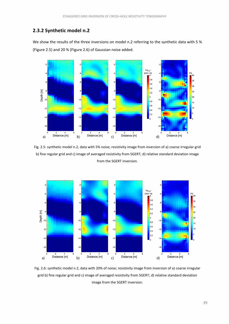
STAGGERED GRID INVERSION OF CROSS‐HOLE RESISTIVITY TOMOGRAPHY
39
2.3.2 Synthetic model n.2
We show the results of the three inversions on model n.2 referring to the synthetic data with 5 %
(Figure 2.5) and 20 % (Figure 2.6) of Gaussian noise added.
Fig. 2.5: synthetic model n.2, data with 5% noise; resistivity image from inversion of a) coarse irregular grid
b) fine regular grid and c) image of averaged resistivity from SGERT; d) relative standard deviation image
from the SGERT inversion.
Fig. 2.6: synthetic model n.2, data with 20% of noise; resistivity image from inversion of a) coarse irregular
grid b) fine regular grid and c) image of averaged resistivity from SGERT; d) relative standard deviation
image from the SGERT inversion.

STAGGERED GRID INVERSION OF CROSS‐HOLE RESISTIVITY TOMOGRAPHY
40
Comparing again the three methods, it can be seen how the SGERT tends to limit the formation of
inversion artefacts at all the noise levels, obtaining smoother images that result to be more
similar to the synthetic model. For model n.2 too, the standard deviation map shows the highest
values in correspondence of the resistivity boundaries and within the high sensitivity areas close
to the boreholes.
Figure 2.7 (model 1), Figure 2.8 (model 2, 5% noise) and Figure 2.9 (model 2, 20% noise)
respectively show the RPE images, obtained for both the single grid and SGERT results, with
reference to Equation (2.3).
Figure 2.7: RPE calculated between the inversion result on the coarse irregular grid (a), on the fine regular
grid (b) and SGERT result (c) on model 1.

STAGGERED GRID INVERSION OF CROSS‐HOLE RESISTIVITY TOMOGRAPHY
41
Figure 2.8: RPE calculated between the inversion result on the coarse irregular grid (a), on the fine regular
grid (b) and SGERT result (c) on model 1 (data with 5% noise).
Figure 2.9: RPE calculated between the inversion result on the coarse irregular grid (a), on the fine regular
grid (b) and SGERT result (c) on model 2 (data with 20% noise).
RPE images show the accuracy of the inversions, where white corresponds to perfect
reconstruction, blue colours and red colours respectively stand for under‐ and over‐estimation of

STAGGERED GRID INVERSION OF CROSS‐HOLE RESISTIVITY TOMOGRAPHY
42
the model resistivity. Even though all the methods show similar RPE distribution, SGERT appears
to be more accurate than single grid inversions in reconstructing the real value from the synthetic
model. This is reflected also from MAD values, from Equation (2.4), reported in Table 1. It can also
be observed that the RPE values are high in the zones of high standard deviation (i.e. in
correspondence of the resistivity boundaries).
Tab. 2.1: MAD values for the three inversion results on the three different synthetic datasets
MAD [ohm m] Fine regular grid Coarse irregular grid Staggered grid
Model 1 123.8654 112.6647 106.9666
Model 2 noise 5% 149.43 163.14 134.3269
Model 2 noise 20% 238.6005 270.9866 225.6439
2.3.3 Field dataset
Figure 2.10 reports the result from the single inversion on the coarse irregular grid (Figure 2.10a),
on the regular fine grid (Figure 2.10b), the average resistivity result of SGERT inversion (Figure
2.10c) and the related standard deviation matrix (Figure 2.10d). The white line indicates the
groundwater level.
Fig. 2.10: Field dataset from Trecate site; a) resistivity image from a grid reflecting the sensitivity
distribution; b) resistivity image from single grid inversion; c) image of averaged resistivity from SGERT; d)
relative standard deviation image from the SGERT inversion.

STAGGERED GRID INVERSION OF CROSS‐HOLE RESISTIVITY TOMOGRAPHY
43
This application of the SGERT on a real dataset improves the result if compared to the ones
obtained with the single inversions. The inversion on the coarse irregular grid tends to spread the
high resistive anomaly located in the depth range between 8 to 11 m, but it well reconstructs the
rest. The inversion on the fine regular grid points out the anomaly but the whole image is blurred
and affected by the presence of artefacts. The tomographic image from the application of SGERT
shows, like the one from the coarse irregular grid, the alternance of conductive and resistive
layers within the vadose zone and the resistivity anomaly in the saturated zone. The relative
standard deviation values are higher in correspondence of the resistivity boundaries and in the
middle of the resistive superficial layer.
We validate the SGERT results with some geological information of the Trecate site (Figure 2.11a),
and to the results of the spectral analysis on a GPR Zero Offset Profile (ZOP) (Figure 2.11b); the
GPR data was collected in the same day. The groundwater level is represented by the horizontal
blue line. The resistive anomaly observed within the depth range of 8 m to 10 m is well related to
the stratigraphy sequence (presence of sand and gravels). The tomographic image also agrees
with the cross‐hole ZOP data. The trend of the spectrum of the received signal at each depth is
pointed out in Figure 10c. Data were collected at depth step of 25 cm. Each amplitude spectrum is
computed by windowing each radar trace using the same time‐window (160 ns). The peak of
energy is observed just below the groundwater level. This founds an interpretation in the
presence of a trapped hydrocarbon emulsion within the smear zone. The behaviour of the
trapped NAPL, which is characterized by high resistivity and low permittivity, is somehow
analogous to that explained in Glaser et al. (2012). In this work, which is about a controlled GPR
lab‐scale test, a controlled release of ethanol in a tank was monitored with a series of GPR
acquisition over time. The highest peaks in the power spectra were observed just below the water
table.

STAGGERED GRID INVERSION OF CROSS‐HOLE RESISTIVITY TOMOGRAPHY
44
Fig. 2.11: a) subsoil stratigraphy at Trecate site (TS: top soil, SSH: silty sand w/ hydrocarbon, SGH: sand and
gravel w/ hydrocarbon, GCS: gravel and coarse sand, CSPH: coarse sand w/ pebbles and hydrocarbon, CSP:
coarse sand w/ pebbles, SG: sand and gravel); b) resistivity image from SGERT at Trecate site, values in log
scale; c) trace‐by‐trace spectrum of the ZOP profile at Trecate site.
The conductive layer between the groundwater level and the resistive layer should correspond to
the level where the hydrocarbon oxidation and bio‐degradation is enhanced by the presence of
fresh air, as the water table rise in summer and is followed by a part of the oil trapped in the
pores. This very thin layer is evidenced also by the high values of standard deviation at the depth
of 8 m, which indicates the presence of two resistivity boundaries, as explained above for the
synthetic cases.
Finally, the conductive superficial layer corresponds to a zone of silt and sand accumulation, as
evidenced by GPR profiles and ERT obtained from previous studies (Godio et al., 2010).
STAGGERED GRID INVERSION OF CROSS‐HOLE RESISTIVITY TOMOGRAPHY
45
2.4 Conclusions A procedure for resistivity data inversion which includes the staggered grid method was herein
discussed. The main goal is to improve the reliability of the inversion by enhancing the S/N ratio
and preserving, in the largest part of the domain, the conditioning of the selected inversion
scheme. Furthermore, we obtain good results inverting several well‐conditioned (or slightly
under‐determined) problems.
We tested the staggered grid procedure on both synthetic and field dataset. The results
confirmed that the SGERT method can be a useful and powerful tool in the inversion of cross‐hole
resistivity data, where sensitivity problems and the presence of noise in the data cannot be
overcome by a traditional single grid inversion and when a‐priori conditions are not available. The
procedure has a different effect on high gradient, e.g. near electrical interfaces, and on
homogeneous zones, e.g. within a layer. In fact by shifting the mesh, the SGERT virtually increases
the resolution and outputs sharper boundaries at the interfaces while, by the averaging
operation, SGERT gives smoother images in the homogeneous zones provoking a reduction of
inversion artefacts. As a consequence of the staggering, we estimate the standard deviation
related to each pixel of the solution allowing for the evaluation of the precision of the final model.
The image of the standard deviation is useful to detect resistivity boundaries in zones of poor
model resolution. The main drawback is the need of performing many inversions which implies an
increase in computational time even though this increase doesn’t depend linearly on the number
of inversion to be carried out. In fact, while performing a single inversion of a real dataset on a
very fine mesh grid takes from 5 to 30 minutes (depending on the complexity of the problem and
on the number of elements in the model), the completion of SGERT process requires from 30 to
90 minutes on a commercial laptop PC, with a 2.2 GHz processor and a 4 GB RAM. The strengths
of the method are, besides the possibility to check the reliability of the solution over the
interested area of the model, to reduce the artefacts and detect more accurately the resistivity
boundaries. The possibility to overcome these problems encourages us to apply the SGERT to the
time‐lapse inversion of electrical resistivity data.

STAGGERED GRID INVERSION OF CROSS‐HOLE RESISTIVITY TOMOGRAPHY
46
References Binley A., 2010. Resistivity Software R2 profile Version 2.6 (November 2010).
Böhm, G., Galuppo, P., Vesnaver, A., 2000. 3D adaptive tomography using Delaunay triangles and
Voronoi polygons: Geophysical Prospecting, 48, 723‐744.
Cassiani, G., Godio, A., Stocco, S., Villa, A., Deiana, R., Frattini, P., Rossi, M., 2009. Monitoring the
hydrologic behaviour of a mountain slope via time‐lapse electrical resistivity tomography, Near
Surface Geophysics, 7, 475‐486.
Davis, K., Li, Y. 2011. Fast solution of geophysical inversion using adaptive mesh, space‐filling
curves and wavelet compression, Geophysical Journal International, 185, 157–166.
Glaser, D.R., Werkema, D.D., Versteeg, R.J., Henderson, R.D., Rucker, D.F., 2012. Temporal GPR
imaging of an ethanol release within a laboratory‐scaled sand tank. Journal of Applied Geophysics,
86, 133‐145.
Godio, A., Naldi, M., 2003. Two dimensional electrical imaging for detection of hydrocarbon
contaminants. Near Surface Geophysics, 1, 131‐137.
Godio, A., Arato, A., Stocco, S., 2010. Geophysical characterization of a nonaqueous‐phase liquid–
contaminated site. Environmental Geosciences 17, pp. 141‐162.
Godio, A., Borsic, A., Arato, A., Sambuelli, S., 2011. On the inversion of cross‐hole resistivity data.
Geophysical Research Abstracts Vol. 13, EGU2011‐7950.
Kemna, A., 2000. Tomographic inversion of complex resistivity—Theory and application, PhD
Thesis, Bochum Ruhr‐Univ., Germany.
Lines, L. R., Treitel, S., 1984. A review of least‐squares inversion and its applications to geophysical
problems, Geophys. Prosp., 32, 159‐186.
Louis F. I., Makropoulos, K. C., Louis, I. F., 2005. Image enhancement in seismic tomography by
grid handling: Synthetic simulations with fault‐like structures, Journal of Balkan Geophysical
Society, 8, 4, 139‐148.
Michelini, A., 1995. An adaptive‐grid formalism for travel‐time tomography: Geophys. J. Int., 121,
489‐510.
Inman, J. R., 1975. Resistivity inversion with ridge regression, Geophysics, 40, 798‐817.
Poletto L., Nicolosi, P., 1999. Enhancing the spatial resolution of a two‐dimensional discrete array
detector, Opt. Eng. 38, 1748‐1757.

STAGGERED GRID INVERSION OF CROSS‐HOLE RESISTIVITY TOMOGRAPHY
47
Sambuelli L., Bohm G., Capizzi P., Cardarelli E., Cosentino P. (2011). Comparison between GPR
measurements and ultrasonic tomography with different inversion algorithms: an application to
the base of an ancient Egyptian sculpture . Journal of Geophysics and Engineering, 8, 106‐116.
Tezkan, B., Georgescu, P., Fauzi, U., 2005. A radiomagnetotelluric survey on an oil‐contaminated
area near the Brazi Refinery, Romania. Geophys. Prospect., 53:311–323.
Tikhonov, A. N., Arsenin, V. Y., 1977. Solutions of Ill‐Posed Problems, Ed. Fritz, J.,Wiley & Sons.Ur,
H., Gross, D., 1992. Improved resolution from subpixel shifted pictures. Graphical Models and
image Processing, 54 (2), 181‐186.
Vesnaver, A., 1996. Irregular grids in seismic tomography and minimum time ray tracing: Geophys.
J. Int., 126, 147‐165.
Vesnaver, A., and Böhm, G., 2000. Staggered or adapted grids for seismic tomography: The
Leading Edge, 19, 944‐950.

48
3. Forward modeling and inversion for 2‐D and 3‐D real/complex electrical resistivity
data
This chapter presents the formulation of a forward/inverse code for 2‐D and 3‐D electrical
resistivity data.
This code has been developed jointly with Dr. A. Borsic (Dartmouth College, Dartmouth, NE)
within the activities of FP7 European Project SoilCAM, and is based on the numerical framework
developed by Borsic and Adler (2012). It can be used on 2‐D and 3‐D Finite‐Element models for
both modelling and inversion of resistivity data, given an arbitrary geometric disposition of the
current sources.
We present preliminary results related to the development of a novel package for 2D and 3D
inversion (called NES‐GeoElectric), for 2D and 3D inversion of electrical resistivity data. The
approach is based on a core of functionalities, as computing the forward solution and the
sensitivity matrix, that are optimized for speed of execution on single‐core and multi‐core
computing platforms. These functionalities have been customized, within the SoilCAM EU FP7
project, for the specific application to subsurface imaging, including functions for automatic mesh
generation given a description of the geometry of the site.
The inversion scheme is based on a Primal Dual‐Interior Point Method (PD‐IPM) framework which
allows using either the L1‐norm or the L2‐norm on the data term and on the regularization term
of the inverse formulation (Borsic and Adler, 2012). Use of the L1‐norm on the data term
corresponds to a Least Absolute Values formulation, which is particularly robust to the presence
of outliers in the data, while use of the L1‐norm on the regularization term corresponds to Total
Variation formulation, which results in sharper reconstructed profiles. Besides the
aforementioned approach, we implemented strategies to improve the accuracy in the forward
model formulation and to reduce the errors that can arise from using simplified models, given
that Electrical Resistivity Tomography (ERT) is an ill‐posed inverse problem. Adaptive meshing or
staggering grid are strategies that can minimize the ambiguities in most ill‐pose problems as well;
Arato et al. (2012, submitted) modified the original staggering grid approach (Michelini, 1995,
Bohm and Vesnaver, 1999) to adapt the multi‐inversion procedure to cross‐hole resistivity data.

FORWARD MODELING AND INVERSION FOR 2‐D AND 3‐D REAL/COMPLEX ELECTRICAL RESISTIVITY DATA
49
In processing of cross‐hole resistivity data, with particular attention towards the monitoring of
dynamic processes in contaminated sites, modelling electrodes with a finite extent covers a
noteworthy importance, as the electrode size is usually not negligible compared to their distance.
Modelling electrodes therefore as point source results in appreciable approximations, and
contributes to poorer reconstructed images. The approach we adopted is focused on building
accurate 2D and 3D forward meshes that account for the presence of the borehole and for the
extent of the electrodes. These are described with a boundary condition known as Complete
Electrode Model (CEM), as it has been taken from previous studies (e.g. Cheng et al., 1989,
Somersalo et al., 1992, Hyvonen, 2004, Rücker and Günther, 2011).The CEM accounts for the
finite size of the electrode and for the non‐uniformity of the current density flow underneath the
surface of the same electrode. This model has been shown experimentally to be able to predict
measured data on electrodes of extended surface to 0.2% accuracy (Borsic, 2002).
The computation of the Jacobian matrix, the most intensive step in our implementation, has been
implemented using calls to the Intel Math Kernel Library (MKL), a multithreaded BLAS and LAPACK
implementation, highly optimized for modern PC architectures. This results in gains in the order of
30 times compared, for example, to the use of plain MATLAB. The forward solution, which
requires solving a sparse linear system, and is the second most expensive step in our algorithm,
has been implemented using the MKL PARDISO (PARAllel DIrect SOlver) solver, which in our tests
is about 10 times faster compared to MATLAB’s sparse solver on modern multicore PCs. These
optimizations are particularly useful in 3D, as accurate modeling of electrodes and of the domain
results in meshes with typically 100,000 to 300,000 nodes, and 500,000 to 1,500,000 tetrahedral
elements.
Finally, the approach allows reconstructing complex resistivity data, when spectral electrical
resistivity data are available and information on the induced polarization over the investigated
medium is required. Both the real and imaginary values of the complex resistivity can be
reconstructed.
3.1 Mesh Generation
In ERT imaging of the subsurface electric fields are applied to the ground by injecting current
through electrodes. The concept behind resulting electric field has very strong spatial variations in
proximity of the electrodes, while it is smooth at a distance. The use of adaptive refinement
schemes is therefore promising in terms of forming meshes that are fine only where needed. As,
particularly in 3D, using dense meshes (e.g. 500,000 nodes) results in a significant computational

FORWARD MODELING AND INVERSION FOR 2‐D AND 3‐D REAL/COMPLEX ELECTRICAL RESISTIVITY DATA
50
effort, optimizations have been made, developing adaptive mesh approaches which guarantee a
good forward accuracy and reduce computing time. We are currently implementing adaptive
mesh refinement schemes, where, given an initial forward solution, a posterior error is estimated
on each element of the mesh and worse elements are refined, leading to a reduction of the
overall forward error. In such a context, Plattner et al. (2012) transfer the adaptive wavelet
approach presented in Cohen et al. (2003) for well posed problems into the realm of
underdetermined electrical resistivity tomography. This allows to generate initial meshes that are
relatively coarse and to refine them only where needed, obtaining significant savings in
computations. Figure 3.1 shows results from tests designed to verify those elements of the mesh
that are correctly split.
Fig. 3.1: Imaging test on adaptive mesh refinement.
We incorporate a series of routines for mesh generation considering a polygonal model of the
imaging domain, of the electrodes, and of any borehole which might be present. Electrodes can
be modelled as points or cylindrical sources, for the latter the Complete Electrode Model (CEM) is
used. Given this geometric representation external mesh generators are used for creating 2D and
3D FEM meshes. We adopt, respectively the public domain software Triangle
(http://www.cs.cmu.edu/~quake/triangle.html) for generating 2D meshes, and TetGen
(http://tetgen.berlios.de/) for generating 3D meshes. As these two mesh generators are
distributed in binary and source code form (C/C++ language), we developed ad‐hoc MATLAB mex‐
files to interface and exchange mesh data with these packages.

FORWARD MODELING AND INVERSION FOR 2‐D AND 3‐D REAL/COMPLEX ELECTRICAL RESISTIVITY DATA
51
The mesh generation provides two different models for the electrodes, in terms of their
geometry. The simplest model is the point electrode. A second model is the cylindrical electrode,
as the ones usually mounted on boreholes. The user specifies the location and the type of
electrode model and an appropriate mesh representative of the geometry and electrode models
is automatically generated. A second customization regards the boundary conditions to be applied
to the mesh, which account for non uniform current density on the surface of electrodes (CEM).
Meshes are extended to a distance from the imaging area, and impedance boundary conditions
are used to simulate an infinite domain. The 2D and 3D mesh generation process allows to model
an arbitrary number and location of boreholes, an arbitrary number of electrodes, considering
their height, diameter and position along the borehole. The coarseness or fineness of the mesh
can be adjusted as well in terms of:
‐ max volume of elements in the background region ;
‐ max volume of elements in the imaging region;
‐ max area of the facets that constitute electrodes.
With respect to Figure 3.2, we refer to the background region as the coarser mesh region which is
used to model the soil volume at a distance from the electrodes. This volume, where a coarser
mesh is generated, allows to approximate, with opportune boundary conditions, an infinite half‐
space. The imaging region presents a finer mesh, as it is the volume limited by the electrodes
array, where the field has faster spatial variations, and where the resistivity is imaged. The
adoption a finer mesh in this region provides for accurate forward solutions. Boreholes are
modelled accounting for the diameter of the borehole and for the true extent of the electrodes.

FORWARD MODELING AND INVERSION FOR 2‐D AND 3‐D REAL/COMPLEX ELECTRICAL RESISTIVITY DATA
52
Fig. 3.2: Example of automatically generated mesh for a 3‐D cross‐hole problem.
3.2 Inversion of complex resistivity datasets Since resistivity can be considered a function of frequency of the electric field applied into the
ground, it is a naturally complex quantity. It has two contributions: one given by the real valued
ground resistivity, and the second dependent on the polarization characteristics of the soil.
Measuring the complex resistivity of a soil means to collect measurements of spectral data, e.g.
amplitude and phase, at different frequencies in the desired frequency range. Resistivity (ρ) can
be considered frequency‐dependent and complex, defined as:
( ) '( ) i "( ) (3.1)
where ω is equal to 2π∙f, and f is the frequency of the injected electrical field.
Recovery of both real and imaginary part of the complex resistivity can give additional information
both regarding the soil constituents and pollutants such as hydrocarbons, which show induced
polarization effects. The method works with real and complex valued field data, recovering
modulus and phase of the complex resistivity, where phase information is available.
The reconstruction routines allow processing complex resistivity datasets, gathered from
frequency domain AC georesistivimeters. The phase and amplitude component of the measured
data can be inverted, reconstructing a tomographic image of the complex resistivity in the domain
of interest, or recovering separately the real and imaginary part of the complex resistivity.
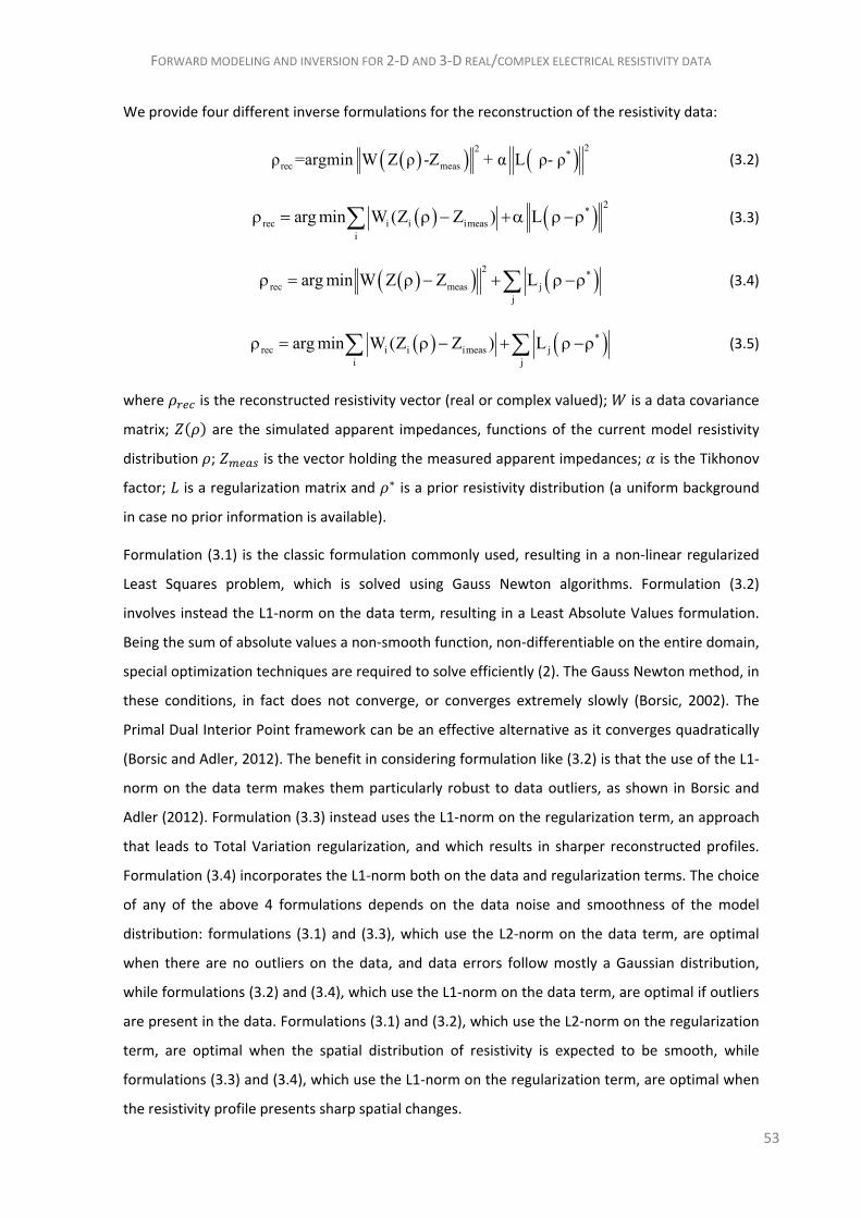
FORWARD MODELING AND INVERSION FOR 2‐D AND 3‐D REAL/COMPLEX ELECTRICAL RESISTIVITY DATA
53
We provide four different inverse formulations for the reconstruction of the resistivity data:
22*
rec measρ =argmin W Z ρ -Z + α L ρ- ρ (3.2)
2*
rec i i imeasi
arg min W (Z Z ) L (3.3)
2 *rec meas j
j
arg min W Z Z L (3.4)
*rec i i imeas j
i j
arg min W (Z Z ) L (3.5)
where is the reconstructed resistivity vector (real or complex valued); is a data covariance
matrix; are the simulated apparent impedances, functions of the current model resistivity
distribution ; is the vector holding the measured apparent impedances; is the Tikhonov
factor; is a regularization matrix and ∗ is a prior resistivity distribution (a uniform background
in case no prior information is available).
Formulation (3.1) is the classic formulation commonly used, resulting in a non‐linear regularized
Least Squares problem, which is solved using Gauss Newton algorithms. Formulation (3.2)
involves instead the L1‐norm on the data term, resulting in a Least Absolute Values formulation.
Being the sum of absolute values a non‐smooth function, non‐differentiable on the entire domain,
special optimization techniques are required to solve efficiently (2). The Gauss Newton method, in
these conditions, in fact does not converge, or converges extremely slowly (Borsic, 2002). The
Primal Dual Interior Point framework can be an effective alternative as it converges quadratically
(Borsic and Adler, 2012). The benefit in considering formulation like (3.2) is that the use of the L1‐
norm on the data term makes them particularly robust to data outliers, as shown in Borsic and
Adler (2012). Formulation (3.3) instead uses the L1‐norm on the regularization term, an approach
that leads to Total Variation regularization, and which results in sharper reconstructed profiles.
Formulation (3.4) incorporates the L1‐norm both on the data and regularization terms. The choice
of any of the above 4 formulations depends on the data noise and smoothness of the model
distribution: formulations (3.1) and (3.3), which use the L2‐norm on the data term, are optimal
when there are no outliers on the data, and data errors follow mostly a Gaussian distribution,
while formulations (3.2) and (3.4), which use the L1‐norm on the data term, are optimal if outliers
are present in the data. Formulations (3.1) and (3.2), which use the L2‐norm on the regularization
term, are optimal when the spatial distribution of resistivity is expected to be smooth, while
formulations (3.3) and (3.4), which use the L1‐norm on the regularization term, are optimal when
the resistivity profile presents sharp spatial changes.

FORWARD MODELING AND INVERSION FOR 2‐D AND 3‐D REAL/COMPLEX ELECTRICAL RESISTIVITY DATA
54
Depending on the characteristics of the data and of the resistivity profile therefore one of the four
formulations is optimal, and can be chosen by the user. A detailed description of the Primal Dual
Interior Point Method framework used for solving (3.2), (3.3), and (3.4) is given in (Borsic and
Adler, 2012).
In the above formulations the covariance matrix of the measurements is used to account for
the uncertainties in the measured apparent impedances, and is built from the users’ specified
standard deviation for each data point. The regularization matrix is a discretization of a first
order differential operator. When used in conjunction with the L1‐norm on the regularization
term, this corresponds to Total Variation regularization. The matrix can be anisotropic (horizontal
or vertical) and specified by the user, in order to better reconstruct resistivity profiles that are
stratified along one direction.
An early release of this approach has been successfully applied to process impedance data of
several controlled experiments on laboratory scale (Borsic et al., 2005), where the electrodes
effect on the final inversion results required a rigorous modelling, and also in processing of data
sets collected in the field.
3.3 Application to synthetic data To illustrate the effect of these choices on the norms to be used we report a series of simulations,
which for simplicity are 2D, but the same results apply in 3D. In 3. 3 a 2D resistivity profile with a
background of 100Ωm and two inclusions of 50 Ωm is shown. A 48 electrodes array was simulated
and placed at the top of the domain and 545 simulated measurements (apparent impedances)
were generated.
Fig. 3.3: Test resistivity profile used for generating synthetic data.
Original noiseless measurements are shown on the left of Figure 3.4. A 5% Gaussian noise was
generated, as well as 20 outliers each one with amplitude of 50 Ω and random sign. These outliers
have been added to the original dataset, as shown in the bottom part of Figure 3.4.

FORWARD MODELING AND INVERSION FOR 2‐D AND 3‐D REAL/COMPLEX ELECTRICAL RESISTIVITY DATA
55
Fig. 3.4: Up) unperturbed synthetic data, bottom) data plus Gaussian noise and 20 outliers.
Figures 3.5 and 3.6 report reconstruction results respectively for data affected only by Gaussian
noise and for data with Gaussian noise and outliers. The figures are organized in 2x2 tables,
showing reconstructions for the four possible combinations on the L1 and L2 norms on the data
and regularization terms of the inverse problem, as in Equations (1), (2), (3), and (4). In the
presence of the Gaussian noise only (Figure 3.5) all formulations work correctly, and the two
reconstructions in the right column, using the L1‐norm as regularization, show a sharp estimation
of the contrasts. When outliers are present, as in simulations of Figure 3.6, inversions based on
the L2‐norm on the data (top row of the table) are sensitive to the outliers, and the estimation is
disrupted by these data errors. The resulting images depend on the value of the Tikhonov factor,
and in all experiments we have optimized the Tikhonov factor in such a way to minimize the RMS
difference between the reconstructed image and the original profile. For each case the
reconstructions represent therefore the best possible result. Reconstructions using the L2‐norm
on the data show therefore how, even optimizing the value of the Tikhonov factor, it is a
challenge to reconstruct the original contrasts. Inversion results based on the L1‐norm on the data
term (bottom row of the table) are instead insensitive to the presence of the outliers. The bottom

FORWARD MODELING AND INVERSION FOR 2‐D AND 3‐D REAL/COMPLEX ELECTRICAL RESISTIVITY DATA
56
left reconstruction (L1 norm on the data and L2 norm on the regularization) can correctly identify
the contrasts and reconstruct, even dough in a smooth way. The reconstruction on the bottom
right (L1 norm on the data and L1 norm on the regularization) can correctly identify the contrasts
and reconstruct them in a sharp manner.
Fig. 3.5: Reconstructions of synthetic data, corrupted only by Gaussian noise for the four possible
combinations of norms in the inverse formulations.
Fig. 3.6: Reconstructions of synthetic data, corrupted by Gaussian noise and outliers for the four possible
combinations of norms in the inverse formulations.
A challenging case concerns a test on a synthetic 3‐D model, which is showed in Figure 3.7 in the
upper and lower figures on the left. Four boreholes are embedded in a homogeneous resistive
half‐space, with a high resistivity anomaly in the middle of the volume delimited by the boreholes.
A 3D triangular mesh is used to simulate the presence of 4 boreholes (two visible and two hidden
in the volume of the mesh itself). A set of synthetic measurements of complex resistivity is
obtained for a dipole‐dipole configuration. We show in Figure 3.7 simulations regarding the
separate recovery of the real and imaginary part of the resistivity.

FORWARD MODELING AND INVERSION FOR 2‐D AND 3‐D REAL/COMPLEX ELECTRICAL RESISTIVITY DATA
57
Fig. 3.7: Synthetic simulation of 3‐D complex resistivity data (model and reconstruction are shown for the
real part and the imaginary part on the top and on the bottom, respectively)
The top left picture shows a purely real contrast present in the top portion of the simulated cross‐
borehole region. The bottom left picture shows an imaginary valued contrast. The two contrasts
where used for simulating complex valued measurements, and fed into the reconstruction
routines. The top right image shows to the real part of the reconstructed resistivity, and the
bottom right picture shows the reconstructed imaginary part of the resistivity. Clearly the
real/imaginary contrasts are well separated and reconstructed. Presently the application to field
data of complex reconstruction is challenging, as for typical values of permittivity of the soil and
of measurement frequencies, the imaginary part of the measured impedances is very small in
value and results in a very poor signal‐to‐noise ratio.
3.4 Application to real cases The performance of the code has been tested on a series of datasets coming from various real
applications. We chose four possible cases, considering 2‐D and 3‐D measurements with electrode
deployments both on ground surface and in cross‐hole fashion. Measurements were carried out
on test‐sites with known characteristics in terms of resistivity distribution.
A set of 2‐D resistivity data has been acquired in 2010 at a research site of the National Research
Council in Torino (Italy). As it can be seen in Figure 3.8, the site mainly consists of a resistivity

FORWARD MODELING AND INVERSION FOR 2‐D AND 3‐D REAL/COMPLEX ELECTRICAL RESISTIVITY DATA
58
anomaly embedded in a homogeneous soil. The anomaly is a real 3‐D feature, a basin filled with
well‐sorted coarse sand (Giubbolini and Sambuelli, 2000). It is highly permeable and mostly dry,
providing high resistivity values if compared with the ones of the surrounding soil, which is mostly
characterized by silty‐sand.
Fig.3.8: Description of the test site the National Research Council (CNR), Turin.
The data were acquired with a 48 electrode array, 1 m spaced, centered on the anomaly. In‐line
electrodes 21 and 26 have been placed at 21 and 26 m, respectively, at the boundaries between
the sand basin and the soil around. A Wenner‐Schlumberger configuration with 545 independent
measures was selected.
For the 2‐D case, we inverted the same dataset using all the four possible combination for the
norms to be used.
The results are presented in Figure 3.9, respectively by solving the problem with Formulation 3.1
(Figure 3.9a), Formulation 3.2 (Figure 3.9b), Formulation 3.3 (Figure 3.9c) and Formulation 3.4
(Figure 3.9d).
The first two images show a smooth representation of the resistive basin, with the second one
without the lateral tail besides the basin, meaning that the L1‐norm has been insensitive to the
presence of some outliers. The L1‐norm on the regularization term gives very sharp results, as
shown in (9c) and (9d).

FORWARD MODELING AND INVERSION FOR 2‐D AND 3‐D REAL/COMPLEX ELECTRICAL RESISTIVITY DATA
59
Fig.3.9: Resistivity images at the CNR tes site, surface 2‐D acquisition. Results coming from Formulation 3.1
(a), 3.2 (b), 3.3 (c) and 3.4 (d), respectively.
The 3‐D dataset was acquired at the same site described above, with a 144 electrode array, which
were disposed as in Figure 3.10, centered on the anomaly. We used a pole‐dipole array, placing
the remote electrode 170 m far from the anomaly in the eastern direction. A data set of 6696
measurements was obtained by considering forward and reverse schemes along x‐ and y‐
direction, and furthermore along the two diagonals.

FORWARD MODELING AND INVERSION FOR 2‐D AND 3‐D REAL/COMPLEX ELECTRICAL RESISTIVITY DATA
60
Fig.3.10: Electrode array for the surface 3‐D survey, with a pole‐dipole configuration, at the CNR test site,
Turin.
In Figure 3.11 the results of the inversion on the surface 3‐D dataset over the sand basin are
presented. This result has been obtained by using the common Least Square implementation,
then assuming Gaussian distribution of the errors over the dataset and a smooth regularization.
The basin is well identified, and we observed high resistivity values down to 2 m, corresponding to
the bottom of the basin. Even the global shape of the anomaly is preserved. On the right side of
the figure some cut‐through slices of resistivity at increasing depth are shown (from the top‐left
corner to the down‐right corner).

FORWARD MODELING AND INVERSION FOR 2‐D AND 3‐D REAL/COMPLEX ELECTRICAL RESISTIVITY DATA
61
Fig. 3.11: Resistivity distribution for the surface 3‐D case, CNR‐Turin test‐site, obtained with a common
Least square formulation (L‐2 norm both on the data and regularization term).
Sharper results on the same dataset were obtained by using the L‐1 norm on the regularization
term. The high contrast in resistivity values between the basin and the soil around permitted to
regularize considering the absolute values on the “model” term, or Total Variation, of the
objective function. In Figure 3.12 it is clear how the sharpness of the resistivity boundaries is
preserved by the inversion, even though the reconstruction doesn’t point out the real depth of
the basin bottom, which is placed at 1.5 m instead of 2 m.
Fig.3.12: Resistivity distribution for the surface 3‐D case, CNR‐Turin test‐site, obtained with the application
of the L‐2 norm on the data term and of the L‐1 norm on the regularization term.

FORWARD MODELING AND INVERSION FOR 2‐D AND 3‐D REAL/COMPLEX ELECTRICAL RESISTIVITY DATA
62
We tested the inversion code to a 3‐D dataset coming from a test‐site which is located in
Gorgonzola, near Milan (Italy). The site belongs to the University of Milano Bicocca (Italy), and it is
made up by three boreholes (b‐A, b‐B and b‐C) which were installed in 2004 (see plan view in
Figure 3.13). Each borehole is equipped with 24 electrodes 0.8 m spaced, in the depth range
between 1.6 to 20 m from ground surface. One additional borehole (b‐D), with no electrodes, was
further installed for monitoring fate and transport processes during pumping tests and infiltration
experiments.
The acquisition has been carried out in January 2011, by utilizing a dipole‐dipole generalized
array; the geological stratification of the site is reported in Figure 3.13.
Fig. 3.13: Description of the geometry (left) and the soil stratigraphy (right) at the Gorgonzola test site.
Figure 3.14 shows the results of the inversion of resistivity data from the cross‐hole 3‐D case. This
result has been achieved by using the common least square inversion, with slight horizontal
anisotropy ratio. A tri‐dimensional rendering of the resistivity distribution is shown on the left,
indicating a resistive layer in the depth range between 6 and 11 m and corresponding to the layer
of gravel with absence of finer material. The superficial and less resistive layer can be related to
the presence of finer sand, while below 12 m a gradual transition towards low resistivity values
indicates the presence of the saturated unconfined aquifer.

FORWARD MODELING AND INVERSION FOR 2‐D AND 3‐D REAL/COMPLEX ELECTRICAL RESISTIVITY DATA
63
Fig. 3.14: Resistivity distribution for the cross‐hole 3‐D case, Gorgonzola test‐site, obtained with a common
Least square formulation (L‐2 norm both on the data and regularization term).
3.5 Discussion and conclusions A general limitation of ERT is the ill‐posedness that image reconstruction presents. Ill‐posedness
can be limited by complementing reconstruction with data available from other sources
(constrained reconstruction, use of prior information) and by using regularization techniques. On
this front different solutions have been adopted in research work and in the software packages
available in the public domain.
Cardarelli et al. (2006), for example, presented a 2D strategy based on an iterative smoothness‐
constrained least‐squares algorithm; their approach ensures flexibility in resolution, by taking into
account an initial arbitrarily defined model. They also introduced a priori information in different
regions of the domain, using inequality constraints. Moreover they provided strategies to refine
the mesh, to control the inversion procedure by a smoothness matrix and for controlling the
regularization parameter (damping) at each iteration. Amongst the available non‐commercial
code, a well known package developed by Andrew Binley (Binley, 2010) performs forward/inverse
solution 2D and 3D solutions using triangular and tetrahedral meshes. The inverse solution is
based on a regularised objective function combined with weighted least squares, the so called
Occam’s type solution (Binley and Kemna, 2005). In comparison to the Binley’s package, our
approach provides a different flexibility in modeling the boreholes effects, allowing the user to

FORWARD MODELING AND INVERSION FOR 2‐D AND 3‐D REAL/COMPLEX ELECTRICAL RESISTIVITY DATA
64
control the mesh density in 2D and 3D and provides several inversion schemes, allowing to choose
the L1 or L2 norm of the data and regularization terms.
Smoothness constrains may lead to bias in the ERT inversion image (Friedel, 2003, Day‐Lewis et
al., 2005). The survey design (quantity and spatial arrangement of measurements), the
distribution of electrical conductivity and the data error are the factors affecting the most the bias
of the inverted image (Day‐Lewis et al., 2005). Methods for solving 3‐D problems often require
significant computational efforts, in solving the sparse linear Equations resulting from the FEM
model (Friedel, 2003; Day‐Lewis et al., 2005) and in the parameter estimation (Yeh et al., 2002):
these methods provide a rather qualitative measure of regions prone to bias, such as sensitivity
analyses (Kemna et al., 2002). The so‐called volume of investigation index (Oldenborger et al.,
2007) may be an alternative to reduce these efforts. The package we presented in this paper aims
at dealing efficiently with the computational cost of 3D solutions, but using 3D meshes that are
adaptive, and by best exploiting modern PC architectures, which are multicore. When the L1 norm
is used, a Primal Dual ‐ Interior Point Method is employed for solving the resulting optimization
problem, a method which is particularly efficient for L1 norm optimization.
The developing of an inversion approach of amplitude and phase of electrical data, including
strategies to model the effects of boreholes and electrodes (in boreholes) represent an
improvement with respect to the conventional approaches, allowing a more rigorous control of
the electrodes and borehole effects on the inversion process with appreciable advantages when
the electrodes’ size is no longer negligible with respect to their distance, as this often occur in
cross‐hole survey.
The overall approach presented in this chapter is implemented in a software package based on
the NES‐GeoElectric library, that allows reconstruction of 2D and 3D electric impedance data
optimized for speed and for parallel operation on multi‐core computing architectures. NES‐Geo‐
Electric has been coded as a Matlab toolbox, with core routines written in C language and
optimized for performance. Our intention is to release soon the NES‐GeoElectric package under a
public domain licence.

FORWARD MODELING AND INVERSION FOR 2‐D AND 3‐D REAL/COMPLEX ELECTRICAL RESISTIVITY DATA
65
References Arato, A., A. Godio and L. Sambuelli, Staggered grid inversion of cross‐hole resistivity data;
submitted to Journal of Applied Geophysics, July, 2012.
Bastani, M., J. Hubert, T. Kalscheuer, L. Pedersen, A. Godio, and J. Bernard, 2012, 2D joint
inversion of RMT and ERT data versus individual 3D inversion of full tensor RMT data. An example
from Trecate site in Italy: Geophysics, 77, WB233‐WB243, DOI: 10.1190/GEO2011‐0525.1.
Binley, A., 2010, Free Resistivity Software R2 version 2.6 Generalised 2‐D Inversion of Resistivity
Data. http://www.es.lancs.ac.uk/people/amb/Freeware/freeware.htm
Binley, A., and A. Kemna, 2005, Electrical Methods, In: Hydrogeophysics by Rubin and Hubbard
(Eds.), 129‐156, Springer.
Bohm, G. and A. Vesnaver, 1999, In quest of the grid: Geophysics, 64, no. 4, 1116–1125.
Borsic, A., and A. Adler, 2012, A Primal Dual ‐ Interior Point Framework for Using the L1‐Norm or
the L2‐Norm on the Data and Regularization Terms of Inverse Problems: Inverse Problems, 28, No.
9, 095011, DOI:10.1088/0266‐5611/28/9/095011.
Borsic, A., C. Comina, S. Foti, R. Lancellotta and G. Musso, 2005, Imaging heterogeneities in sand
samples with Electrical Impedance Tomography: laboratory results: Geotechnique, 55, 539‐647.
Borsic A., 2002, Regularization methods for imaging from electrical measurements. PhD Thesis,
Oxford Brookes University, October 2002.
Bouchedda, A., M. Chouteau, A. Binley, B. Giroux, 2012, 2‐D Joint structural inversion of cross‐
hole electrical resistance and ground penetrating radar data: Journal of Applied Geophysics, 78,
52‐57.
Cassiani, G., V. Bruno, A. Villa, N. Fusi and A. M. Binley, 2006. A saline tracer test monitored via
time‐lapse surface electrical resistivity tomography, Journal of Applied Geophysics , 59, No. 3,
244‐259.
Cassiani G., A. Godio, S. Stocco, A. Villa, R. Deiana, P. Frattini and M. Rossi, 2009, Monitoring the
hydrologic behaviour of a mountain slope via time‐lapse electrical resistivity tomography: Near
Surface Geophysics, 7 , 475‐486.
Cardarelli E., and F. Fischanger, 2006, 2D data modelling by electrical resistivity tomography for
complex subsurface geology: Geophysical Prospecting, 54, No. 2, 121–133, DOI: 10.1111/j.1365‐
2478.2006.00522.x

FORWARD MODELING AND INVERSION FOR 2‐D AND 3‐D REAL/COMPLEX ELECTRICAL RESISTIVITY DATA
66
Cheng K. S., D. Isaacson, J. C. Newell, and D. G.Gisser, 1989, Electrode Models for Electric Current
Computed Tomography: IEEE Transactions in Biomedical Engineering, 36, No. 9, 918‐924.
Cohen, A., W. Dahmen, and R. DeVore, 2003, Adaptive wavelet schemes for nonlinear variational
problems: SIAM J. Numerical Analysis, 41, No. 5, 1785–1823.
Comina, C., and L. Sambuelli, 2012, Geoelectrical measurements for agricultural canal seepage
detection: Proceedings Near Surface Geoscience 2012 ‐18th Meeting on Environmental and
Engineering Geophysics ‐ Paris, 3‐5 Sep., paper n. C.34, 5pp.
Day‐Lewis, F. D., K. Singha, and A. M. Binley, 2005, Applying petrophysical models to radar travel
time and electrical resistivity tomograms: Resolution‐dependent limitations: Journal of
Geophysical Research, 110, B08206, DOI:10.1029/2004JB003569.
Friedel, S., 2003, Resolution, stability and efficiency of resistivity tomography estimated from a
generalized inverse approach: Geophysical Journal International, 153, 305–316.
Giubbolini L., and L. Sambuelli, 2000, New developments in ground probing radar: the possibility
of reconstruction of a holographic image of underground reflectivity: Annali di Geofisica, 43,
1105‐1118.
Godio A., and M. Naldi, 2003, Two dimensional electrical imaging for detection of hydrocarbon
contaminants: Near Surface Geophysics, 1, 131‐137.
Godio A., and S. Ferraris, 2005, Time lapse geophysics for monitoring an infiltration test in vadose
zone: Bollettino di Geofisica Teorica e Applicata, 46, 201‐216.
Godio A., and M. Naldi, 2009, Integration of Electrical and Electromagnetic Investigation for
Contaminated Site: American Journal of Environmental Sciences, 5, 561‐568, ISSN: 1553‐345X.
Godio, A., A. Arato, and S. Stocco, 2010, Geophysical characterization of a nonaqueous‐phase
liquid–contaminated site: Environmental Geosciences, 17, 141‐162.
Godio, A., A. Borsic, A. Arato, and L. Sambuelli, 2011, On the inversion of cross‐hole resistivity
data: Geophysical Research Abstracts, 13, EGU2011‐7950.
Hyvonen, N., 2004, Complete electrode model of electrical impedance tomography:
approximation properties and characterization of inclusions: SIAM Journal on Applied
Mathematics, 64, No. 3, 902–931.
Kemna A., B. Kulessa, and H. Vereecken, 2002, Imaging and characterisation of subsurface solute
transport using electrical resistivity tomography (ERT) and equivalent transport models: Journal of
Hydrology, 267, 125‐146.

FORWARD MODELING AND INVERSION FOR 2‐D AND 3‐D REAL/COMPLEX ELECTRICAL RESISTIVITY DATA
67
Kemna A., A. Binley, and L. Slater, 2004, Crosshole IP imaging for engineering and environmental
applications: Geophysics, 69, No. 1, 97‐107.
LaBrecque, D.J., G. Morelli, W. Daily, A. Ramirez, and A. Lundegard, 1999, Occam's inversion of 3‐
D electrical resistivity tomography: in Three‐Dimensional Electromagnetics, 575–590, eds
Oristaglio, M. & Spies, B., Soc. Expl. Geophys., Tulsa , OK.
Maurer, H. and S. Friedel, 2006, Outer‐space sensitivities in geoelectrical tomography,
Geophysics, 71, No. 3, G93–G96.
Michelini, A., 1995, An adaptive‐grid formalism for travel‐time tomography: Geophysical Journal
International, 121, No. 2, 489–510.
Morelli, G. and D.J. LaBrecque, 1996, Advances in ERT inverse modeling: European J.
Environmental and Engineering Geophysics, 1, 171–186.
Oldenborger, G.A., P.S. Routh, and M.D. Knoll. 2007, Model reliability for 3D electrical resistivity
tomography: Application of the volume of investigation index to a time‐lapse monitoring
experiment: Geophysics, 72, F167–F175.
Plattner, A., H. R. Maurer, J. Vorloeper, and M. Blome, 2012, 3‐D electrical resistivity tomography
using adaptive wavelet parameter grids: Geophysical Journal International, 189, 317–330,
DOI:10.1111/j.1365‐246X.2012.05374.x.
Rücker, C. and T. Günther, 2011, The simulation of finite ERT electrodes using the complete
electrode model: Geophysics, 76, No. 4, F227‐F238, DOI: 10.1190/1.3581356.
Sambuelli, L., L. V. Socco, A. Godio, G. Nicolotti, and R. Martinis, 2003, Ultrasonic, electric and
radar measurements for living trees assessment: Bollettino di Geofisica Teorica ed Applicata, 44,
No. 3‐4, 253‐279.
Somersalo, E., M. Cheney and D. Isaacson, 1992, Existence and Uniqueness for Electrode Models
for Electric Current Computed Tomography: SIAM Journal on Applied Mathematics, 52, No. 4,
1023‐1040.
Strobbia C., A. Godio, and G. De Bacco, 2006, Interfacial waves analysis for the geotechnical
characterization of marine sediments in shallow water: Bollettino di Geofisica Teorica e Applicata,
47, 145‐162.
Tikhonov, A. N., and V. Y. Arsenin, 1977, Solutions of Ill‐Posed Problems: Winston & Sons
Washington D.C.

FORWARD MODELING AND INVERSION FOR 2‐D AND 3‐D REAL/COMPLEX ELECTRICAL RESISTIVITY DATA
68
Yeh, T.C.J., S. Liu, R. J. Glass, K. Baker, J. R. Brainard, D. Alumbaugh, and D. LaBrecque, 2002, A
geostatistically based inverse model for electrical resistivity surveys and its applications to vadose
zone hydrology: Water Resources Research, 38, No. 12, 1278, http: //dx.doi.org
/10.1029/2001WR001204.

69
4. Time‐lapse inversion of electrical resistivity data
This chapter is aimed to furnish an overview of the basics of inversion of resistivity data in time‐
lapse fashion, with further applications of a novel method on synthetic and real 2‐D cross‐hole
data.
The dynamic characterization of a site is necessary when the inference of variations of
geophysical parameters with time is needed. ERT, particularly in cross‐hole configuration due to
limited lack of resolution with depth, is a reliable technique for long‐term monitoring of the
effects of the groundwater fluctuations of an unconfined superficial aquifer in a contaminated
site. Superficial water resources are the first sensible target of anthropogenic contamination, and
this reason encouraged many authors (e.g. Slater et al., 2000; Cassiani et al., 2006) to study the
applicability of ERT for monitoring controlled field infiltration tests. The results of such these tests
provided qualitative and quantitative information on hydrological parameters of the soil, which
mainly control flow and transport phenomena through the aquifer geological formations. Other
authors (e.g. Godio and Naldi, 2003; Atekwana et al., 2004a, 2004b, 2004c, 2004d) have
investigated the application of ERT to characterize and monitor hydrocarbon contaminated sites.
4‐D analysis of electrical resistivity data has to take into account a series of factors that contribute
to the overall spatial and temporal variability of the resistivity distribution in the considered soil
system. Particular importance has to be attributed to those phenomena influencing the pore‐fluid
saturation and the fluid composition, under the assumption of invariance of the electrical
characteristics of the soil matrix.
The most simple method for understanding the temporal behaviour of resistivity with ERT is to
compare inversion results making the ratio of inverted resistivity from two subsequent datasets.
However, this method can introduce severe errors in the interpretation of time‐lapse changes. In
fact, each resulting image is diversely affected by inversion artefacts that come from
measurement errors and systematic errors (due, for instance, to misplacement of the electrodes),
which are usually augmented by the optimization process.

TIME‐LAPSE INVERSION OF ELECTRICAL RESISTIVITY DATA
70
In order to overcome this problem, Daily et al. (1992) proposed the so‐called ratio method, with
consists in inverting the dataset of fictitious resistances
tr hom
0
RR R(F )
R (4.1)
where the ratio resistance dataset is made up by dividing dataset of resistances at time t (Rt) with
respect to the background dataset R0, and multiplying this ratio by a synthetic dataset of
resistance values R(Fhom). R(Fhom) comes from the solution of the direct problem for an electrically
homogenous half‐space, i.e. with constant resistivity of ρhom. The result of the inversion of Rr show
a distribution of resistivity whose values are higher or lower than ρhom in correspondence of the
zones of increment or decrement of resistivity from time 0 to time t. However, the ratio method
only gives qualitative information on the resistivity changes, and it is difficult to give a quantitative
interpretation of the time‐lapse results.
Miller et al. (2008) proposed what they called “cascaded” time‐lapse inversion algorithm.
Cascaded inversion uses the result of a single inversion of the background dataset as starting and
reference model during the inversion. The main hypothesis is that the resistivity distribution
doesn’t change significantly with time, thus the subsequent model can be considered similar to
the background model. The minimization is based on the difference between the model at time t
and the background resistivity model, and the smoothing is applied to the difference between the
two subsequent models, instead of being placed as a constraint to the second model. Naturally,
this approach is robust when changes in the electrical condition of the soil system are small
between the different time‐steps.
A slightly different approach was studied by LaBrecque and Yang. (2001), who developed a time‐
lapse difference inversion method which is aimed to minimize the data differences from two
subsequent datasets, and the difference between the forward response of the two models. As in
Miller et al. (2008), the method requires a background resistivity model which comes from the
inversion of the background dataset.
Both the cascaded and the difference method are then sensitive to noise amplification (artefacts)
during inversion of the background datasets, and the solution of the time‐lapse differences can be
affected by artefacts from the background inversion result.
In 2009 Kim et al. provided a new formulation for time‐lapse inversion, adding a parameter into
the objective function to account for the temporal resistivity variations. The prerogative of this
method is the assumption of temporal linearity, meaning that the global electrical characteristics
of the investigated medium change linearly between one time step to the subsequent one.

TIME‐LAPSE INVERSION OF ELECTRICAL RESISTIVITY DATA
71
Hayley et al. (2011) developed a time‐lapse method based on the concept of the spatially
constrained inversion, in order to ensure smooth changes from subsequent time steps. The
smoothness constraints are placed within a single optimization problem, claiming for a limitation
of the propagation artefacts from the background model.
Our necessity of dealing with systems characterized by highly dynamic changes forced us to find
simple but reliable methods to perform time‐lapse analysis of electrical resistivity data.
In Chapter 2.2, a demonstration of the possibility to check the precision of inversion result from
SGERT has been provided. We take advantage from this peculiarity with the aim to apply the
SGERT to time‐lapse analysis of electrical resistivity data.
In presence of artefacts in the resulting image on the background dataset, unreal resistivity
changes will propagate in the differences with respect to subsequent times. The best the
definition of the background resistivity model is, the more reliable the time‐lapse differences will
be. As previously presented, the SGERT produces two resulting matrix, representing the
distribution of average resistivity and the related standard deviation.
Standard deviation distribution is indicative of the precision (i.e. repeatability) of the inversion in
each of the pixels resulting from the staggering and re‐sampling of the different grids used for
SGERT.
High standard deviation values were found in correspondence of high model sensitivity zones
(mostly near the electrodes and along the boreholes) and in zones differently reconstructed on
the various grids. This occurs along resistivity boundaries and in areas of the model where the
resistivity features were inconsistent. For this reason, SGERT are usually characterized by less
artefacts.
4.1 Application of SGERT to time‐lapse Electrical Resistivity
Tomography
The possibility to account for the precision of the final resistivity inversion, pixel per pixel, using
the relative standard deviation distribution, encouraged us to use SGERT method for the inversion
of time‐lapse resistivity data. Obviously, standard deviation (referred to as σ, which has not to be
confounded here with electrical conductivity) is intimately linked to the average resistivity
distribution, since the grid staggering operates in a different way on the same dataset but on the
different grids in the staggering process.
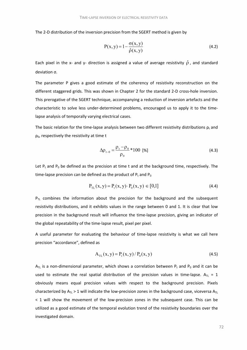
TIME‐LAPSE INVERSION OF ELECTRICAL RESISTIVITY DATA
72
The 2‐D distribution of the inversion precision from the SGERT method is given by
(x, y)
P(x, y) 1ˆ(x, y)
(4.2)
Each pixel in the x‐ and y‐ direction is assigned a value of average resistivity , and standard
deviation σ.
The parameter P gives a good estimate of the coherency of resistivity reconstruction on the
different staggered grids. This was shown in Chapter 2 for the standard 2‐D cross‐hole inversion.
This prerogative of the SGERT technique, accompanying a reduction of inversion artefacts and the
characteristic to solve less under‐determined problems, encouraged us to apply it to the time‐
lapse analysis of temporally varying electrical cases.
The basic relation for the time‐lapse analysis between two different resistivity distributions ρt and
ρ0, respectively the resistivity at time t
t 0t 0
0
*100
[%] (4.3)
Let Pt and P0 be defined as the precision at time t and at the background time, respectively. The
time‐lapse precision can be defined as the product of Pt and P0
TL t 0P (x, y) P (x, y) P (x, y) ]1,0[ (4.4)
PTL combines the information about the precision for the background and the subsequent
resistivity distributions, and it exhibits values in the range between 0 and 1. It is clear that low
precision in the background result will influence the time‐lapse precision, giving an indicator of
the global repeatability of the time‐lapse result, pixel per pixel.
A useful parameter for evaluating the behaviour of time‐lapse resistivity is what we call here
precision “accordance”, defined as
TL t 0A (x, y) P (x, y) / P (x, y) (4.5)
ATL is a non‐dimensional parameter, which shows a correlation between Pt and P0 and it can be
used to estimate the real spatial distribution of the precision values in time‐lapse. ATL = 1
obviously means equal precision values with respect to the background precision. Pixels
characterized by ATL > 1 will indicate the low‐precision zones in the background case, viceversa ATL
< 1 will show the movement of the low‐precision zones in the subsequent case. This can be
utilized as a good estimate of the temporal evolution trend of the resistivity boundaries over the
investigated domain.

TIME‐LAPSE INVERSION OF ELECTRICAL RESISTIVITY DATA
73
4.2 Joint use of staggered grid and difference inversion
We used the difference inversion algorithm proposed by LaBrecque and Yang (2001), encoded in
the R2 package code (Binley, 2010).
As stated in the previous paragraph, difference inversion is an extension of the traditional
Occam’s inversion, carried out by minimizing the objective function ψ(m)
T T(m) = D D + ( - ) ( - ) D 0 0W m m R m m (4.6)
where WD is the data weighting matrix, α is the damping factor, R the model regularization (or
roughness) matrix, while m and m0 correspond to the model parameter vectors at time t and 0,
respectively.
The vector parameter m0 comes from a single inversion of the background dataset, and
constitutes the starting and the reference model for the difference inversion process.
The data difference vector in the objective function of Equation (4.6) has the form
D = ( - ) - [g( ) - g( )] obs obs0 0d d m m (4.7)
where dobs and g(m) represent the data vector and the forward response for the model m,
respectively, and the subscript index “0” denotes the background dataset and forward response.
The model update Δm=mk+1‐mk is obtained by solving the following Equation as an optimization
problem, usually with a conjugate‐gradient approach,
T Tk D k k D k( ) = ( - ) 0J W J R m J W D R m m (4.8)
where J is the Jacobian (i.e. sensitivity) matrix.
Difference inversion is computationally efficient since the method is based on the calculation of
one Jacobian matrix, which is supposed to describe adequately the sensitivity distribution of both
the model at time t and the background model. This assumption implies that the resistivity
changes are not so great, and the process is oriented to find small perturbation with respect of
the initial model.
However, LaBrecque and Yang (2001) demonstrated the effectiveness of the method in reducing
inversion artefacts on real cases with highly contrasting resistivity layers, dealing with time‐lapse
data characterized by great resistivity changes and high percent of noise.

TIME‐LAPSE INVERSION OF ELECTRICAL RESISTIVITY DATA
74
For this reason we make use of joint SGERT method with difference inversion algorithm (named
SGDERT in the following) for highly dynamic environments, combining the benefits of difference
inversion and the effect of time‐lapse precision assessment coming from SGERT.
To demonstrate the effectiveness of this approach, we apply it both on synthetic and real cross‐
hole data.
4.3 Application to synthetic data
The performance of the SGDERT technique is evaluated by inverting datasets from two very
simple synthetic time‐lapse cases, shown in Figure 4.1 and Figure 4.2.
The electrode arrangement is the same as in 2‐D cross‐hole cases presented in chapter 2.
The first synthetic time‐lapse case represents a common geological situation of sedimentary
superficial aquifers, with a resistive (1000 ohm m)sandy layer overhanging a saturated half‐space
with a bulk resistivity of 100 ohm m. Any effect of smoothing due to the presence of a capillary
fringe is neglected in these particular cases. The time‐lapse resistivity evolution simulates the rise‐
up of the water table, from a depth of 9 to 6 m below the ground surface. The opposite situation
characterizes the second time‐lapse case, which simulates the water level drop from a depth of 6
to 9 m below ground surface (b.g.s).
The time‐lapse differences for the two cases are completely different, with 90% negative relative
decrease in the oscillation zone for the first case, while the resistivity increase in the second case
implies a positive relative increase of about 900%.

TIME‐LAPSE INVERSION OF ELECTRICAL RESISTIVITY DATA
75
a) b) c)
Fig. 4.1: Synthetic time‐lapse model n. 1: a) background resistivity; b) resistivity at time t; c) relative
resistivity difference.
a) b) c)
Fig. 4.2: Synthetic time‐lapse model n. 2: a) background resistivity; b) resistivity at time t; c) relative
resistivity difference.
Two separate data sets of 1200 resistance values (in Ω) were obtained for a pole‐dipole array. We
inverted the synthetic dataset using the R2 code fixing a data error to be slightly conservative (i.e.
imposing error level slightly greater than the real error level in the data from the forward
solution) on the real error level on the data. We choose the maximum number of iteration to be
equal to 10. The optimal smoothing factor is updated by the code at each iteration, and it was

TIME‐LAPSE INVERSION OF ELECTRICAL RESISTIVITY DATA
76
properly set to have a smooth model along the horizontal direction, as it is usually done to follow
the horizontal geological layers.
a) b)
c) d)
Fig. 4.3: Synthetic time‐lapse model n. 2 (noise‐free data), results from the SGERT inversion: image of
average resistivity for the background (a) and the subsequent (c) case, precision P0 (b) and Pt (d).

TIME‐LAPSE INVERSION OF ELECTRICAL RESISTIVITY DATA
77
Results of the SGDERT on the first synthetic model are shown in Figure 4.3. Figure 4.4 reports the
time‐lapse resistivity differences and the time‐lapse precision and accordance.
a) b) c)
Fig. 4.4: Synthetic time‐lapse model n. 1 (noise‐free data), results from the SGERT inversion: image of (a)
time‐lapse percent resistivity difference (b) time‐lapse precision PTL and c) precision accordance.
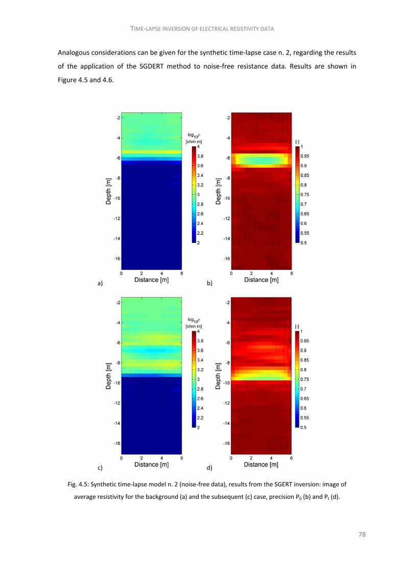
TIME‐LAPSE INVERSION OF ELECTRICAL RESISTIVITY DATA
78
Analogous considerations can be given for the synthetic time‐lapse case n. 2, regarding the results
of the application of the SGDERT method to noise‐free resistance data. Results are shown in
Figure 4.5 and 4.6.
a) b)
c) d)
Fig. 4.5: Synthetic time‐lapse model n. 2 (noise‐free data), results from the SGERT inversion: image of
average resistivity for the background (a) and the subsequent (c) case, precision P0 (b) and Pt (d).

TIME‐LAPSE INVERSION OF ELECTRICAL RESISTIVITY DATA
79
a) b) c)
Fig. 4.6: Synthetic time‐lapse model n. 2 (noise‐free data), results from the SGERT inversion: image of (a)
time‐lapse percent resistivity difference (b) time‐lapse precision PTL and c) accordance.
The same approach has been applied to the same time‐lapse cases, whose resistance data had
been added of 10% Gaussian noise.

TIME‐LAPSE INVERSION OF ELECTRICAL RESISTIVITY DATA
80
a) b)
c) d)
Fig. 4.7: Synthetic time‐lapse model n. 1 (10% noise data), results from the SGERT inversion: image of
average resistivity for the background (a) and the subsequent (c) case, precision P0 (b) and Pt (d).

TIME‐LAPSE INVERSION OF ELECTRICAL RESISTIVITY DATA
81
a) b) c)
Fig. 4.8: Synthetic time‐lapse model n. 1 (10% noise data), results from the SGERT inversion: image of (a)
time‐lapse percent resistivity difference (b) time‐lapse precision PTL and c) accordance.
The presence of noise on the data heavily affects the reconstruction, since the inversion method
is a common least square formulation. Then the overall geometry arrangement of the electrical
strata is preserved, and addressed by the precision and accordance distributions, but the method
shows some limits in giving an accurate estimate of the resistivity differences.
Results of the application of SGDERT to the noisy data from the second synthetic case are shown
in Figure 4.9 and 4.10.

TIME‐LAPSE INVERSION OF ELECTRICAL RESISTIVITY DATA
82
a) b)
c) d)
Fig. 4.9: Synthetic time‐lapse model n. 2 (10% noise data), results from the SGERT inversion: image of
average resistivity for the background (a) and the subsequent (c) case, precision P0 (b) and Pt (d).

TIME‐LAPSE INVERSION OF ELECTRICAL RESISTIVITY DATA
83
a) b) c)
Fig. 4.10: Synthetic time‐lapse model n. 2 (10% noise data), results from the SGERT inversion: image of (a)
time‐lapse percent resistivity difference (b) time‐lapse precision PTL and c) accordance.
4.4 Application to real data
The SGDERT method is applied to time‐lapse data coming from Trecate site, contaminated by
LNAPL after a oil‐well blow out. The site is described in Chapter 2.
The resistivity changes with time at Trecate site are mainly governed by water table fluctuations.
The contaminated site is located in an agricultural area characterized by an intensive irrigation
activity, which starts in the early spring and terminates in the late summer. The superficial un‐
confined aquifer is directly influenced by this hydraulic forcing condition, with a consequent
seasonal variation of the water table of 4‐5 meters.
Even so, vertical aquifer recharge in correspondence of the test‐site is not direct, because of a
very low permeable clayey layer on the surface. It occurs through apposite infiltration pits located
100 m away from the test‐site.
The time‐lapse datasets herein used cover a period of time that ranges from April, 2010 to
February, 2011. This is a sub‐set of the whole data recorded at the site, in a time frame from
August 2009 to May 2012. Four time steps are considered: April 2010, July 2010, October 2010
and February 2011. The choice of this four time‐steps was made with the aim of covering 1 year
period, with a with a quite homogeneous distribution of the campaigns over the four seasons. The
objective of the study is to evaluate the sensitivity of time‐lapse ERT in following the piezometric
level oscillations and the consequent LNAPL smearing. Thus, resistivity data from the April 2010

TIME‐LAPSE INVERSION OF ELECTRICAL RESISTIVITY DATA
84
campaign has been chosen as background, because of the lowest level of the water table at that
time. Borehole direct measurements placed the water depth at 10 m from the surface.
Results from the SGERT inversion of the April 2010 dataset are shown in Figure 4.11.
a) b)
Fig. 4.11: resistivity data from Trecate site, April 2010: image of (a) averaged resistivity and (b) precision P
image from the SGERT inversion. White dashed line indicates water table level. This resulting resistivity is
used as background for the time‐lapse inversion.
The resistivity panel in Figure 4.11 (a) points out three main resistivity horizons, one conductive
layer on the top of the images, an alternance of resistive layers from 3 to 10 m b.g.l., overlying a
conductive half‐space. Those main layers respectively correspond to an upper silty layer, to an
inhomogeneous vadose zone above the water table, and to the lower saturated zone, where no
significant contamination has been found below 11 m b.g.l..
The result of the SGERT inversion on April 2010 data has been used as background for the SGDERT
method, described above and applied to the datasets of July 2010, October 2010 and February
2011.
Results of the time‐lapse SGDERT method are shown in Figures 4.12 to 4.17, organized as the
ones from the synthetic cases.
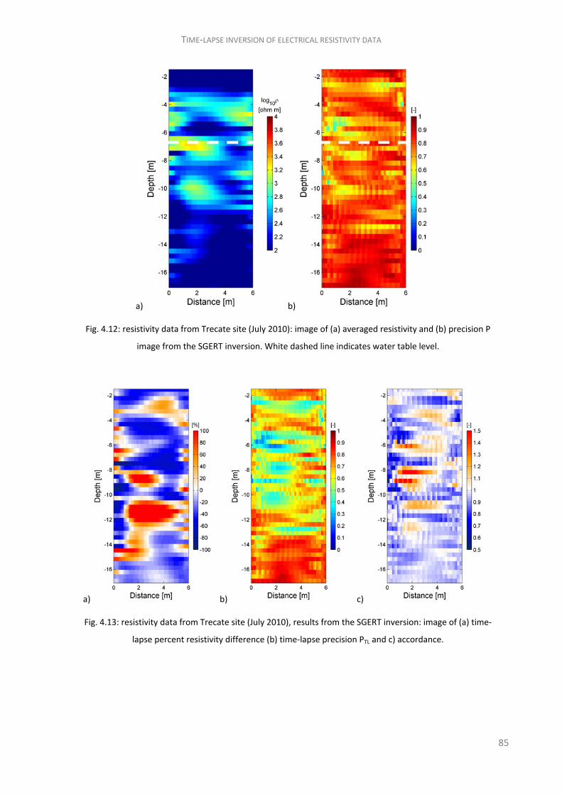
TIME‐LAPSE INVERSION OF ELECTRICAL RESISTIVITY DATA
85
a) b)
Fig. 4.12: resistivity data from Trecate site (July 2010): image of (a) averaged resistivity and (b) precision P
image from the SGERT inversion. White dashed line indicates water table level.
a) b) c)
Fig. 4.13: resistivity data from Trecate site (July 2010), results from the SGERT inversion: image of (a) time‐
lapse percent resistivity difference (b) time‐lapse precision PTL and c) accordance.

TIME‐LAPSE INVERSION OF ELECTRICAL RESISTIVITY DATA
86
a) b)
Fig. 4.14: resistivity data from Trecate site (October 2010): image of (a) averaged resistivity and (b) precision
P image from the SGERT inversion. White dashed line indicates water table level.
a) b) c)
Fig. 4.15: resistivity data from Trecate site, October 2010; results from the SGERT inversion: image of (a)
time‐lapse percent resistivity difference (b) time‐lapse precision PTL and c) accordance.
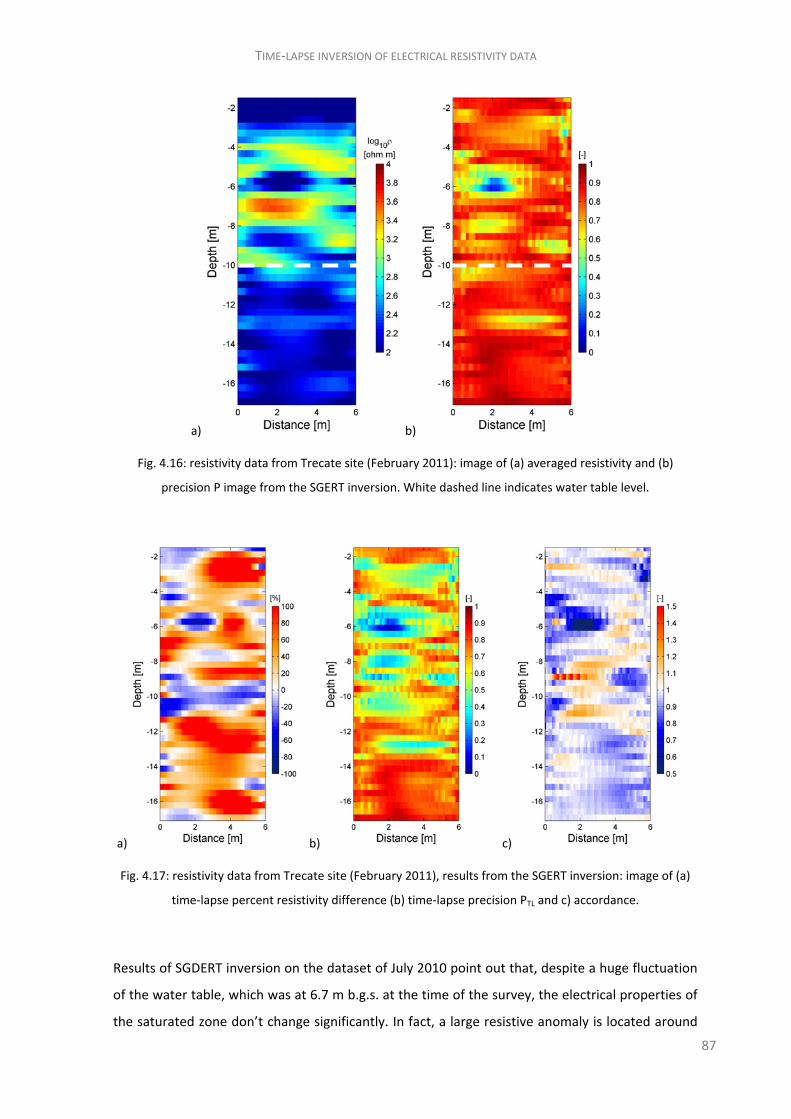
TIME‐LAPSE INVERSION OF ELECTRICAL RESISTIVITY DATA
87
a) b)
Fig. 4.16: resistivity data from Trecate site (February 2011): image of (a) averaged resistivity and (b)
precision P image from the SGERT inversion. White dashed line indicates water table level.
a) b) c)
Fig. 4.17: resistivity data from Trecate site (February 2011), results from the SGERT inversion: image of (a)
time‐lapse percent resistivity difference (b) time‐lapse precision PTL and c) accordance.
Results of SGDERT inversion on the dataset of July 2010 point out that, despite a huge fluctuation
of the water table, which was at 6.7 m b.g.s. at the time of the survey, the electrical properties of
the saturated zone don’t change significantly. In fact, a large resistive anomaly is located around

TIME‐LAPSE INVERSION OF ELECTRICAL RESISTIVITY DATA
88
the depth of 10 m. this can’t be explained by differences in the geological stratification. Deeper
than 8 m (which is a layer richer in silt composition, up to 10%) the aquifer is mainly compounded
by gravel and coarse sand. The most realistic hypothesis is that, considering that 11 m was the
water table depth at the time the accident occurred, the oil reached this depth with no possibility
to move further down. This caused the formation of a very oil‐rich horizon (Atekwana et al.,
2009), and the great water fluctuations created a smearing of the LNAPL. Then, in case of higher
water table levels, we have a smear zone with high concentration of trapped oil; in the resistivity
image this yields a resistive feature embedded in the most conductive zone (the saturated level).
The time‐lapse evolution of the overall geometry of the problem is also reflected in the precision
and accordance distributions.
Results of dataset of October 2010 show a similar response with respect to the background case,
both concerning the spatial distribution and the resistivity values (accordance values are, as a
consequence, close to 1). In fact, resistivity difference is quite low, apart from the fluctuation
layer between 8 and 10 m b.g.s..
February 2011 data were themselves higher, and the inversion results reflect this peculiarity.
Again, the geometrical reconstruction of the resistivity strata is similar to the background case,
but the resistivity value are quite high all over the section, when compared with the background
values. This is reflected by the relative percent difference values, with higher resistivity value even
in the deep saturated zone.
4.5 Conclusions
This Chapter has showed a novel approach for the inversion of time‐lapse resistivity data, made
up by combining the difference inversion algorithm (LaBrecque and Yang, 2001) and the SGERT
method presented in Chapter 2.
The combination of an efficient method for time‐lapse ERT inversion with a method to verify the
consistency of the resulting resistivity distribution, allowed to test the reliability of the overall
time‐lapse inversion process. The resulting matrices are an average resistivity distribution and
precision, both for the background and the subsequent dataset. Then, accompanying the relative
percentage difference, the SGDERT method furnishes information about the time‐lapse precision,
which is obtained by Equation 4.4 as the product between the static precision for the background
and subsequent cases. This parameter assumes importance in the time‐lapse analysis of resistivity
data, because the method allows to take into account the precision of the inversion of the
background data and even its influence on the inversion of the subsequent data.

TIME‐LAPSE INVERSION OF ELECTRICAL RESISTIVITY DATA
89
Finally, the precision accordance (Equation 4.5) can be utilized for checking the evolution of the
spatial disposition of resistivity layers in the subsoil. In fact, where ATL is greater than the unity,
the background precision is dominating, and we can observe the geometry of the background
case. Viceversa, for ATL values lower than 1, precision values from the subsequent case prevail,
giving an indication of the movement of the resistivity boundaries with time. This is of particular
importance to point out the most significant resistivity boundaries, even when many
inhomogeneities are present in the result.
The SGDERT method has been tested on two synthetic datasets, one simulating a 3m‐raise of the
water table (i.e. corresponding to a resistivity decrease from 1000 to 100 Ω∙m) and the other
simulating the opposite case (i.e. corresponding to a resistivity decrease from 100 to 1000 Ω∙m).
The SGDERT method worked quite well on both clean synthetic data and on resistance data added
by 10% of gaussian noise. Of course, applying a data weighting matrix to account for the 10% data
errors provoked a smoother result, and this was also indicated by the ATL distribution. In fact, it
was more difficult to highlight the true sharp resistivity boundary.
The time‐lapse method was also tested on real data coming from a NAPL‐contaminated site.
Results from the time‐lapse analysis of resistivity data collected at Trecate site give a significant
contribution to the comprehension of the resistivity variation phenomena on a very challenging
real situation. In fact, it was possible to verify the precision of the background resistivity model,
and to check for the time‐lapse precision and accordance for the subsequent cases. In this real
case, precision inversion is lower than in results of synthetic data inversion, and this information
has to be taken into account when making quantitative interpretation of the results.

TIME‐LAPSE INVERSION OF ELECTRICAL RESISTIVITY DATA
90
References Binley, A., 2010. Resistivity Software R2, profile Version 2.6 (November 2010).
Cassiani, G., Bruno, V., Villa, A., Fusi N., and Binley, A. M., 2006. A saline tracer test monitored via
time‐lapse surface electrical resistivity tomography. Journal of Applied Geophysics, 59, No. 3, 244‐
259.
Daily, W.D., Ramirez, A.L., LaBrecque, D.J., Nitao, J., 1992. Electrical resistivity tomography of
vadose water movement. Water Resources Research, 28, 1429‐1442.
Hayley, K., Pidlisecky, A., Bentley, L.R., 2011. Simultaneous time‐lapse electrical resistivity
inversion. Journal of Applied Geophysics, 75(2), 401‐411.
Kim, J H., M J. Yi, S G., Park, and J.G. Kim, 2009. 4 D inversion of DC resistivity monitoring data
acquired over a dynamically changing earth model, Journal of Applied Geophysics 68,522‐532.
La Brecque, D. J., Yang, X., 2001. Difference inversion of ERT data: a fast inversion method for 3‐D
in situ monitoring. Journal of Environmental and Engineering Geophysics, 6, 83–89.
Miller, C. R., Routh, P., Brosten, T., McNamara, J., 2008. Application of time‐lapse ERT imaging to
watershed characterization. Geophysics, 73(3), 7‐17.
Slater, L., A.M. Binley, W. Daily, R. Johnson, 2000. Cross‐hole electrical imaging of a controlled
saline tracer injection, Journal of Applied Geophysics, 44, pp. 85–102.

91
5. Integration of geophysical and geochemical data for the characterisation of
biological degradation at an aged LNAPL‐contaminated site
The experimental activity presented in this chapter has been carried out at Trecate site over a two
year time period, from 2009 to 2011. After a preliminary geophysical characterization of the site
(2008‐2009), described in Godio et al. (2010), a test‐site for cross‐hole monitoring has been set‐up
in December 2008 within the most contaminated area of the site.
The test‐site has been specifically designed to monitor time‐lapse changes in electromagnetic
properties both in the vadose and in the saturated zone. More specifically, it has been specifically
designed for cross‐hole ERT and GPR, and completed with two PVC screened boreholes (2”
diameter), named B‐S3 and B‐S4 as they were installed under the framework of EU project
SoilCAM. The two boreholes are 6 m spaced and reach a depth of 18 m b.g.s.. The two boreholes
allow to perform cross‐hole GPR surveys and even geochemical monitoring of groundwater
quality, with multi‐electrode probes. Each borehole addressed with 24 electrodes, 0.7 m spaced,
from the depth of 1 m to 17.1 m b.g.s..
In December 2009, a multi‐level sampling system has been installed in the vicinity of B‐S3 and B‐
S4. Solinst Continuous Multi‐channel Tubing (CMT) system has been set up in Jena and installed
in‐situ with a direct push Geoprobe device. The CMT system consists of 4 multi‐channel
boreholes, with 7 separate micro‐tubes in each. A transect of twenty‐eight sampling ports is then
available for mapping vertically and horizontally the most important physico‐chemical parameter
of interstitial filling fluid in the saturated zone.
From the drilling of two boreholes of the CMT system, soil columns were extracted in transparent
PVC liners, for laboratory characterization of lithological features, presence of contaminant and
laboratory measurements of chemico‐physical parameters.
In addition, microbial count analysis and in vitro growth experiments were performed to assess
the presence of active colonies of hydrocarbon‐degrading bacteria.

INTEGRATION OF GEOPHYSICAL AND GEOCHEMICAL DATA FOR THE CHARACTERISATION OF BIOLOGICAL DEGRADATION AT AN AGED LNAPL‐CONTAMINATED SITE
92
5.1. Material and methods
5.1.1 Geophysical characterization
Several geophysical surveys have been carried out at the SoilCAM test‐site. More specifically, 1‐D
and 2‐D electrical resistivity measurements have been performed on a monthly base. In‐hole
resistivity and IP logs were acquired shifting the quadripole along the total length of the
boreholes. We used a Wenner configuration, with a=0.7 m (i.e. the electrode separation). 2‐D
resistivity tomography have been performed with a pole‐dipole array, using the 48 electrodes
along the two boreholes and a 49th electrode as the remote pole, which was placed 300 m far in
the eastern direction.
Measurements have been carried out with the complex resistivity device, PASI Polares, previously
described in Chapter 2.
Measured resistance and phase data from 1‐D borehole profiles are just transformed to apparent
resistivity and phase logs, while the 2‐D complex impedance data have been inverted using the
framework presented in Chapter 3.
A least‐squares minimization formulation is used, then the L2‐norm is minimized on both the data
and the regularization term of the Occam’s objective function.
5.1.2 Monitoring of chemico‐physical parameters in soil and groundwater
samples
To better understand the small scale geophysical response at the test‐site, two measurement
campaigns of the major chemico‐physical parameters were carried out in October 2010 and May
2011.
The analysis of soil samples involved a grain size characterization, water content measurements
(and derivation of related quantities such as bulk electrical conductivity and bulk dielectric
permittivity), pH, Cation Exchange Capacity (CEC) and measurements of Total Carbon (TC), Total
Organic (TOC) and Total Inorganic Carbon (TIC). Analysis of metal oxides, such as Fe, Mn and Al,
were also performed.

INTEGRATION OF GEOPHYSICAL AND GEOCHEMICAL DATA FOR THE CHARACTERISATION OF BIOLOGICAL DEGRADATION AT AN AGED LNAPL‐CONTAMINATED SITE
93
Groundwater sampling was carried out at very low flow rate with submersible double valve
pumps, at the sampling ports of the multi‐channel system. Each port was previously depurated
from stagnant water by means of pumping several litres of water with a peristaltic pump.
To avoid oxygen exchange through air and the sample, the double‐valve pumps were operated
with nitrogen gas. During the second campaign some samples had to be drawn with air pressure
again, due to lack of nitrogen gas. To avoid sample cross contamination, pumps and tubings were
cleaned thoroughly between two sampling events in a tested procedure. Additionally to the
multilevel piezometers, a well located outside the contaminated zone was sampled in order to
derive the background values.
Dissolved oxygen, electrical conductivity, redox potential, pH and CO2 was analyzed on‐line in
flow through‐cells with ion selective electrodes (WTW, Weilheim) during pumping on site. Nitrate
(NO3‐), Nitrite (NO2
‐), Sulfide (S2‐), Iron (Fe2+), Manganese (Mn2+; only for the 2nd campaign) and
turbidity were determined photometrically on site immediately after sampling. Samples for
laboratory analysis were kept refridgerated immediately after sampling during all time.
Sulfate(SO42‐) and Chloride (Cl‐) were analysed in the laboratory with ion chromatography. The
samples were filtered in the laboratory with a 0.45 µm filter with supor membrane and acidified
immediately after sampling. Total organic carbon (TOC) and dissolved organic carbon (DOC) was
determined as non‐purgeable organic carbon. Samples were acidified immediately after sampling
and DOC samples were filtered with a 0.45µm filter.
5.1.3 Microbial counts of bacteria in below‐ground soil layers in Trecate
Microbial counts and growth experiments have been performed on several contaminated and
uncontaminated samples from the Trecate site (Figure 5.1), in the laboratories of the RISSAC
(Budapest, Hungary). Samples at different depths were analyzed in order to obtain a vertical
distribution of the bacterial degrading activity.

INTEGRATION OF GEOPHYSICAL AND GEOCHEMICAL DATA FOR THE CHARACTERISATION OF BIOLOGICAL DEGRADATION AT AN AGED LNAPL‐CONTAMINATED SITE
94
Fig. 5.1: Location of sampling points for laboratory biological analysis.
The isolation and enumeration of soil microorganisms were performed using the dilution plate‐
counting technique. For each depth, two series of diluted specimens were used, for the
estimation of both aerobic and anaerobic microbial components in the soil samples.
The catabolic enzymatic activity, through which is possible to infer the presence of extra‐cellular
enzymes and thus to verify the presence of additional sources of energy, was characterized by
Fluorescent diacetate hydrolysis (FDA). FDA consists of a colourless transformation to colours
fluorescein by both free and membrane‐bound bacterial enzymes. FDA hydrolysis was measured
because it is related to general microbiological activity, as stated by Villányi et al. (2006).
Furthermore, the measure of FDA activity provides a description of the microbiological state of
the soils, and can be compared to the amount of the contaminants (Domonkos et al. 2009).
0 25 50 [m]

INTEGRATION OF GEOPHYSICAL AND GEOCHEMICAL DATA FOR THE CHARACTERISATION OF BIOLOGICAL DEGRADATION AT AN AGED LNAPL‐CONTAMINATED SITE
95
5.2 Results and discussion
We present here the results of the integrated geophysical and geo‐chemical characterization at
the contaminated site of Trecate.
The chemico‐physical analysis points out high values of TOC (both in soil and groundwater) and
DOC in the depth range between 8 to 12 m; this states a high NAPL concentration as organic
substrate. Moreover, values of Fe++, manganese, hydrogen carbonate exceeding background
values by far, and low redox potential values were detected, indicating that a degradation activity
is still in progress.
5.2.1 Borehole 1‐D profiling
Results of 1‐D apparent resistivity and IP logs are shown in Fig. and Fig. , for the borehole B‐S3 and
B‐S4 respectively.
Fig. 5.2: borehole B‐S3. Logs of apparent electrical resistivity (a), apparent chargeability (b). Colored bars on
the right side of panel (a) indicate water table level at each time‐step.

INTEGRATION OF GEOPHYSICAL AND GEOCHEMICAL DATA FOR THE CHARACTERISATION OF BIOLOGICAL DEGRADATION AT AN AGED LNAPL‐CONTAMINATED SITE
96
Fig. 5.3: Borehole B‐S4. Logs of apparent electrical resistivity (a), apparent chargeability (b). Colored bars on
the right side of panel (a) indicate water table level at each time‐step.
It is clear from plots of Figures 5.2 and 5.3 that the electrical behaviour, in particular the IP
response, of the two boreholes of the test‐site is dramatically different.
The resistivity profiles point out three main levels:
‐ a conductive layer at the top, corresponding to a silty superficial layer;
‐ a medium resistive layer above the piezometric surface, which presents oscillations due to
various fluid saturation, and probable hydrocarbon smearing;
‐ a conductive layer below the water table, corresponding to the saturated zone.
It has to be noted that the vertical resistivity profiles are quite insensitive of the water table
fluctuations, and especially in B‐S3 the resistivity values tend to decrease only below 12 m b.g.s..
IP logs show a complex behaviour, in particular along the borehole B‐S3. It is reasonable to
neglect IP effects encountered above the water table, because of well known capacitive effects
from bad electrode‐ground contact which originate anomalous and fictitious polarization
responses. The main significant apparent IP anomaly is in the depth range between 8 to 12 m
b.g.s.. It is interesting to notice the accordance between the position of the IP peak and the water
table level.
On the contrary, almost null IP values were found in B‐S4.

INTEGRATION OF GEOPHYSICAL AND GEOCHEMICAL DATA FOR THE CHARACTERISATION OF BIOLOGICAL DEGRADATION AT AN AGED LNAPL‐CONTAMINATED SITE
97
There is a good correlation between apparent chargeability measures and phase values from
complex resistivity measurements. In Figure 5.4 an example of the application of Equation 1.12 is
presented for vertical logs in borehole B‐S3 (dataset acquired in February 2011). Log of apparent
chargeability measured with a DC georesistivimeter (IRIS Syscal Pro) is compared to logs of
apparent phase angle, measured in the frequency range of [0.5‐100 Hz] with Polares. It is worthy
to notice that inductive coupling effects perturb the phase measurements in the vadose zone,
provoking a phase response which can’t be considered indicative of the true phase values of the
surrounding soil.
In the following, complex resistivity data are inverted using NES geoelectric software, in order to
obtain 2‐D tomographic images of the subsoil between boreholes B‐S3 and B‐S4.
Fig. 5.4: comparative plot of vertical phase and chargeability logs (February 2011), related through Equation
(1.12).

INTEGRATION OF GEOPHYSICAL AND GEOCHEMICAL DATA FOR THE CHARACTERISATION OF BIOLOGICAL DEGRADATION AT AN AGED LNAPL‐CONTAMINATED SITE
98
5.2.2 2‐D complex resistivity tomography
2‐D inversion of complex resistivity data can provided useful information of the bi‐dimensional
distribution of resistivity and phase in the transect between borehole B‐S3 and B‐S4. This can help
to understand the anomalous differences in the apparent geophysical response between the two
boreholes.
Inversion results, shown in Figures 5.5 and 5.6, point out a lateral variability in both the module
and phase of the complex resistivity, even for the October 2010 data and for the May 2011 data.
The inversion process of the 2‐D data greatly reduces the overall IP values, and the anomalies in
B‐S3 are in the order of ‐10 mradians, in the depth range between 6 to 10 m.
a) b)
Fig. 5.5: October 2010. Module (a) and phase (b) of the complex resistivity (1.79 Hz) distribution at Trecate
site. The white dashed line indicates the level of the piezometric surface.
The resulting map of complex resistivity for the dataset of May 2011 shows a relatively more
prominent phase response, with a phase anomaly extended at a depth of 12 m b.g.s.. It is
interesting to notice that the groundwater level is almost the same for the two campaigns, but
the global electrical properties in the section is different between the two time series. This is
mainly due to the fact that, after a maximum depth of 11 m b.g.s. reached at the end of February

INTEGRATION OF GEOPHYSICAL AND GEOCHEMICAL DATA FOR THE CHARACTERISATION OF BIOLOGICAL DEGRADATION AT AN AGED LNAPL‐CONTAMINATED SITE
99
2011, the piezometric level is being forced to raise as a consequence of the abundant amount of
water used for irrigation of the fields.
This huge rise produces the so‐called “smearing” of the free phase of the hydrocarbon, and is
responsible for the origin of an isolated blob of trapped LNAPL (Atekwana et al., 2009). This, in
addition to the recharging fresh water from irrigation, can contribute to enhance bio‐degradation
processes of the available organic matter (i.e., the LNAPL).
a b)
Fig. 5.6: May 2011. Module (a) and phase (b) of the complex resistivity (1.79 Hz) distribution at Trecate site.
The white dashed line indicates the level of the piezometric surface.
In fact, the bulk resistivity below the water table is globally higher than in October, and a phase
anomaly can be distinguished at a depth of 11 m b.g.s..

INTEGRATION OF GEOPHYSICAL AND GEOCHEMICAL DATA FOR THE CHARACTERISATION OF BIOLOGICAL DEGRADATION AT AN AGED LNAPL‐CONTAMINATED SITE
100
5.2.3 Distribution of chemico‐physical parameters
Figure 5.7 and Figure 5.8a shows the TOC and DOC concentrations in the groundwater during three
sampling campaigns in the four piezometer wells BS5 to BS8 and in the solid phase (Figure 5.8b).
Fig. 5.7: TOC and DOC in the three sampling campaigns (green 1st , blue 2nd and yellow 3rd campaign) in the
four wells. The background values are indicated by the wells in the uncontaminated location. The first
campaign is not treated in the integrated analysis (Courtesy M. Wehrer, Jena).
The difference between TOC and DOC in the groundwater is a good representative of free phase
oil in the groundwater. Figure 5.6 shows that it is obviously located in large amounts in depths of
around 8.5 m to 10m on each of the three campaigns. On campaign 2 and 3, this depth is just
below the groundwater level, during campaign 1 groundwater level is more than 1.5m higher.
Obviously, a large amount of oil remains in place, despite the large groundwater fluctuations. The
buoyancy of the oil in the groundwater is not large enough that the oil floats on top of the water
level. It is also not completely trapped as residual phase, because in the depths from 8.5m to 10m
free phase oil was discovered. It is important to note that the large TOC concentrations are quite
variable and depend very much on the pumping conditions, so it is difficult to delineate and
amount of free phase present in the groundwater.

INTEGRATION OF GEOPHYSICAL AND GEOCHEMICAL DATA FOR THE CHARACTERISATION OF BIOLOGICAL DEGRADATION AT AN AGED LNAPL‐CONTAMINATED SITE
101
Figure 5.8: TOC a) in the groundwater in the ports of BS5 to BS8 on three sampling campaigns and b) in the
solid phase of liners from BS 5 and BS 7. Area of the circles corresponds to TOC concentration in mg/l in the
pore water. Background values were measured in the uncontaminated location, about 200m distance far
(Courtesy M. Wehrer, Jena).
Below 10 m the amount of free phase is greatly reduced with a quite sharp boundary and most of
the hydrocarbons are present as dissolved phase (at least droplets<0.45µm) with diminishing
concentrations towards deeper zones. The depth of 10m also coincides with the groundwater
level beginning of February, which was the month when the oil blowout occurred. It seems that
the present situation is still highly influenced by the initial conditions of the spreading oil
immediately after the blowout. From Figure 5.8a) it can be assumed that the extension of the
residual NAPL phase may be located more in the direction of well BS8. However, the data is a little
sparse for such a conclusion. Figure 5.8b shows that TOC concentrations in the solid phase (which
correspond to NAPL contamination in deeper layers) generally correspond to the TOC
concentrations measured in the groundwater. It seems, however, that the layer of oil
contamination is spread over a larger area than 8.5m to 10m. It may be that the groundwater
-15
-14
-13
-12
-11
-10
-9
-8
-7
-6
-5
Dep
th
-1 0 1 2 3 4 5
x Position
Fläche der Kreise:TOC
Ref. BS5 BS6 BS7 BS8

INTEGRATION OF GEOPHYSICAL AND GEOCHEMICAL DATA FOR THE CHARACTERISATION OF BIOLOGICAL DEGRADATION AT AN AGED LNAPL‐CONTAMINATED SITE
102
concentrations reflect rather the presence of free phase oil, while from the solid phase
concentrations alone it is not possible to distinguish trapped NAPL and free phase.
Generally, degradation of hydrocarbons results in the production of CO2, when hydrocarbons are
completely mineralized. CO2 dissolves in water and forms carbonic acid, which dissociates into
protons and hydrogen carbonate (measured as Total Inorganic Carbon). This lowers the pH and
increases the electrical conductivity of the pore water. Also, other ionic species are produced
during oxidation of hydrocarbons by different electron acceptors. First, oxygen and nitrate are
depleted. Then, manganese and iron oxides are reduced, which results in the production of
manganese and iron ions. Subsequently, sulfate is reduced to sulfide species and finally
methanogenic conditions may occur. The occurrence of the relevant species is shown in Figure
5.9.
It can be seen that the microbiological activity results in most pronounced changes of the
geochemistry in the depths from 8.5m to 11m. In this area, the microbial activity leads to a
change of conductivity of the pore water, which may be observable by ERT. More pronounced
than for TOC, it seems that the zone of largest activity is shifted towards BS8 (Figure 5.9).
However, the whole observed aquifer is affected, which can be seen in redox sensitive species
and also in the redox potential. Concomitantly to the production of TIC, the redox sensitive
species iron and manganese show their most pronounced increases in the depths from 8.5m to
11m. Shown are the concentrations of total iron, which is mostly Fe2+. Manganese is not shown
here but it is highly correlated with iron. Nitrate and nitrite (both not shown here) are mostly
below detection limit and sulfate concentrations are greatly reduced compared to the background
concentration, almost over the entire depth of the water column (not shown). Only small
amounts of sulfide were detected, which cannot explain the missing sulfate. It seems that other
reduced sulfur species are more abundant, for example HS‐ or H2S, which is to be expected at a
circumneutral pH. Consequently, the conditions can be characterized as ferrogenic on the limit to
sulfidogenic.
Figure 5.9 show a data interpolation of the most relevant chemico‐physical parameter of the
contaminated groundwater:

INTEGRATION OF GEOPHYSICAL AND GEOCHEMICAL DATA FOR THE CHARACTERISATION OF BIOLOGICAL DEGRADATION AT AN AGED LNAPL‐CONTAMINATED SITE
103
a) b)
c) d)
Fig. 5.9: 2‐D interpolation from punctual data of a) specific resistivity, b) TOC concentration, c) Fe++ ion
concentration and d) Mn++ concentration.

INTEGRATION OF GEOPHYSICAL AND GEOCHEMICAL DATA FOR THE CHARACTERISATION OF BIOLOGICAL DEGRADATION AT AN AGED LNAPL‐CONTAMINATED SITE
104
5.2.4 Microbial Counts
Results of microbial counts are presented for the sampling position S1 and S4, respectively
located outside the contaminated area and in the vicinity of the test‐site used for geophysical and
geochemical monitoring. Figure 5.10 and Figure 5.11 show respectively the microbial counts for
both the aerobic and anaerobic microbes.
Fig. 5.10: Colony Forming Units for aerobic microbes, measured at different depths in the sampling point S1
(left) and S4 (right) (Courtesy B. Biró, RISSAC, Budapest).
From the bar‐plot of Figure5.10 it is clear that no significant differences on aerobic microbe CFUs
can be found in S4 with respect to the uncontaminated location. More interesting is the
information coming from counting of anaerobic biomass colonies, in Figure 5.11. The production
of metallic ions is indicative of anoxic, and anaerobic, conditions and then anaerobic bacteria find
in this reductive environment optimal place to grow. Anaerobic CFUs are more than two order of
magnitude greater than the anaerobic CFUs in the control location.
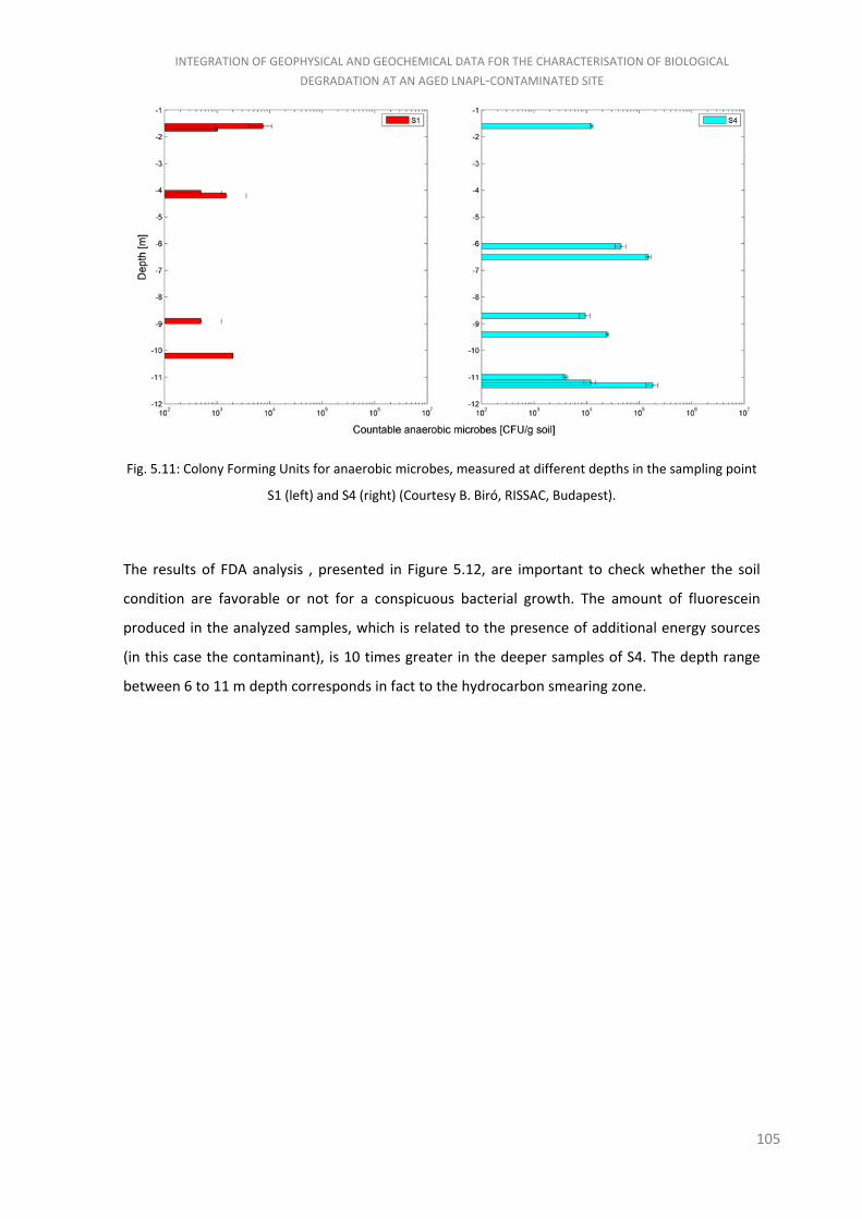
INTEGRATION OF GEOPHYSICAL AND GEOCHEMICAL DATA FOR THE CHARACTERISATION OF BIOLOGICAL DEGRADATION AT AN AGED LNAPL‐CONTAMINATED SITE
105
Fig. 5.11: Colony Forming Units for anaerobic microbes, measured at different depths in the sampling point
S1 (left) and S4 (right) (Courtesy B. Biró, RISSAC, Budapest).
The results of FDA analysis , presented in Figure 5.12, are important to check whether the soil
condition are favorable or not for a conspicuous bacterial growth. The amount of fluorescein
produced in the analyzed samples, which is related to the presence of additional energy sources
(in this case the contaminant), is 10 times greater in the deeper samples of S4. The depth range
between 6 to 11 m depth corresponds in fact to the hydrocarbon smearing zone.

INTEGRATION OF GEOPHYSICAL AND GEOCHEMICAL DATA FOR THE CHARACTERISATION OF BIOLOGICAL DEGRADATION AT AN AGED LNAPL‐CONTAMINATED SITE
106
Fig. 5.12: Fluorescein Diacetate Analysis, measured at different depths in the sampling point S1 (left) and S4
(right) (Courtesy B. Biró, RISSAC, Budapest).
5.3 Conclusions The integrated characterization of the hydrocarbon‐contaminated site of Trecate permitted to
achieve a complete knowledge of the various and complex phenomena which are undergoing at
the site. The results of the geophysical surveys (both ERT and vertical resistivity and IP logs)
pointed out anomalous response in the saturated upper saturated zone, in the depth range
between 8 to 11 m b.g.s.. Despite an expected resistivity decrease, and low IP values, the
tomographic survey pointed out an altered zone, whose values are neither dependent on
different geological features nor on differences in fluid saturation. The zone is then interested by
huge water fluctuations during on a yearly base, responsible for the smearing of the free
hydrocarbon phase which is present in a huge amount.
This hypothesis coming from the interpretation of the geophysical characterization was in good
agreement with the results of the chemico‐physical monitoring. It demonstrated, through the
measure of the Total Organic Carbon and the Total Petroleum Hydrocarbons, that the smearing
zone is the most contaminated level at the site, and that those products serve as additional
source for biological degradation. From a chemical point of view, this has been addressed by the
presence of metabolic by‐products such as Fe++ and Mn++, in an anoxic and reductive
environment. The results of micro‐biological laboratory analysis come to support this thesis,
INTEGRATION OF GEOPHYSICAL AND GEOCHEMICAL DATA FOR THE CHARACTERISATION OF BIOLOGICAL DEGRADATION AT AN AGED LNAPL‐CONTAMINATED SITE
107
indicating that the smearing zone is rich of anaerobic bacteria. Both CFUs and enzymatic activity
tests pointed out that there is an abundance of microbial communities and that the smearing
zone is rich of additional organic matter for the bacteria to proliferate.
References Domonkos, M., 2009. Vertical and horizontal evaluation of pollutants in airport soils.
(Szennyezőanyag vertikális és horizontális értékelése repülőtéri talajban). Diploma work,
University Szent István, SZIE MKK, Gödöllő. (in Hungarian).
Godio, A., Arato, A., Stocco, S., 2010. Geophysical characterization of a nonaqueous‐phase liquid–
contaminated site. Environmental Geosciences 17, pp. 141‐162.
Villanyi, I., Füzy, A., Angerer, I., Biró, B., 2006. Total catabolic enzyme activity of microbial
communities. Fluorescein diacetate analysis (FDA). In: Understanding and modelling plant‐soil
interactions in the rhizosphere environment. Handbook of methods used in rhizosphere research.
Chapter 4.3. Microbiology, Biochemistry and molecular biology. p. 441‐442.

108
CONCLUSIONS
Besides the traditional usages, such as mineral exploration and hydrogeological characterization,
electrical resistivity and induced polarization methods are widely accepted for being, amongst the
large number of geophysical techniques, the most suitable for environmental applications. In fact,
due to their sensitivity to pore fluid saturation and interstitial fluid composition, at small to
medium scale, and thanks to their capability to stimulate “induced” responses in soils, fluids and
in the living part of the subsoil (i.e., the microorganisms), they are usually preferred for the
characterization of contaminated sites. Also, a new branch of geophysics, called “bio‐geophysics”,
gained a great popularity in the last decade, utilizing electrical and electromagnetic methods to
infer the bio‐degradation processes which undergo at contaminated sites.
The research activity presented in this thesis has been focused on the application of electrical and
electromagnetic techniques for geological, hydrological and environmental characterization of
contaminated sites, with particular attention on hydrocarbon contamination.
In this context, one of the purposes was to improve the reliability of the information resulting
from geophysical inversion, when used to support integrated characterization and/or remediation
strategies. Then, innovative approaches have been developed with the aim of reducing the
possible non‐uniqueness of the solution of the geophysical inverse problems. Knowing that, by
definition, geophysical inverse problems are ill‐posed and ill‐conditioned, we worked on the
possibility to check for the consistency of the resulting resistivity image, coming from various
inversion on different FEM grids on the same dataset. The main goal of the Staggered Grid
Electrical Resistivity Tomography (SGERT) approach is actually to improve the reliability of the
inversion by enhancing the S/N ratio and preserving, in the largest part of the domain, the
conditioning of the selected inversion scheme. Stated that the resistivity value has to be constant
in each element of a FEM mesh, the grid staggering has a different effect on homogeneous
resistivity zones and in correspondence of high‐gradient limits. Furthermore, the averaging
operation allows to reduce the formation of possible inversion artifacts. The standard deviation
distribution, pixel per pixel, permits to evaluate the reliability of the resulting resistivity
distribution, and to highlight the presence of the predominant resistivity boundaries. In fact
SGERT, presented in chapter 2, has been shown to be a useful technique for site characterization.

CONCLUSIONS
109
SGERT has been also applied to time‐lapse resistivity data, jointly with the advantages of the
difference inversion algorithm proposed by LaBrecque and Yang (2001). Difference inversion is
computationally efficient and it has been demonstrated to provide good results in many different
situations, both in cases of slowly changing environments and when the data differences reflected
huge variations in the geo‐electrical properties of the subsoil. The combination of difference
inversion and SGERT gives the possibility for the user to check the static and time‐lapse precision
of the results, by analyzing the precision and accordance information. The first one indicates the
level of repeatability of the inversion result on the different grids, while the second one can be
used to interpret the spatial (i.e. geometrical) changes of resistivity distribution over time. Those
two parameter can be effectively used when quantitative information has to be retrieved by geo‐
electrical measurements.
Another approach has been developed with the aim of improving the robustness of the inversion
procedure, in terms of sensitivity to the presence of outliers in the data and of a more rigorous
solution of the direct problem. A novel software for inversion of complex resistivity data, based on
the Primal‐Dual Interior Point formulation, has been tested in Chapter 3 on both synthetic and
real datasets. The software allows a mathematically flexible approach on the search for the
optimal solution (i.e. the minimization of the objective function), by choosing either the L1‐ or the
L2‐ norm on both the data and regularization term of the objective function to be minimized.
Results confirmed that the use of L2‐ norm on the data term is effective on normally distributed
data, and a least square regularization offers a smooth resistivity distribution. Instead, the L1‐
norm is much more robust in presence of outliers in the data, and its use on the regularization
term acts to preserve sharp resistivity boundaries.
A more rigorous solution of the direct problem comes from the internal mesh generator, which
builds triangular or tetrahedral FEMs (in 2‐D or 3‐D) and accounts also for the finite extent of the
electrodes and the boreholes. In fact, appropriate boundary conditions have been set up on the
electrode surface, from which the current is injected non‐uniformly into the ground.
Moreover, the possibility to invert complex resistivity data, makes the code a useful tool for
environmental characterization of contaminated sites. Imaginary part of the complex resistivity
(coming from the measure of the phase shift between current and potential sinusoids) is
influenced by the presence of polarizing materials (such as silt and clay), degradation by‐products
and the degrading activity of the present microbial communities.
In the last Chapter, the integrated characterization of the hydrocarbon‐contaminated site of
Trecate is treated. Geophysical, chemico‐physical and biological methods are combined together
to provide a complete description of the contamination and of the bio‐degradation phenomena

CONCLUSIONS
110
occurring at the site. In‐hole logs and 2‐D resistivity and IP sections have been used to map the
distribution of electrical properties in the subsoil, at metric scale. To support the geophysical
anomalies, measures of the most relevant chemico‐physical parameters, such as Total Organic
Carbon, Total Petroleum Hydrocarbon, iron and manganese ions, have been carried out. High
values of Total Petroleum hydrocarbon have been found in correspondence of the resistive
anomalies, while high values of anaerobic degradation by‐products gave a convincing explanation
to the weird induced polarization response. Laboratory measure of biological colonies counting
and enzymatic activity showed that the site is interested by a slow natural degradation of the
contaminant.
The integrated characterization approach, made up by adding information from various and
independent techniques, permitted to obtain a very complete description of the situation for the
analyzed case study. This comes from the possibility to combine the strength and, more
important, to make up the limits of the different methods.

![Untitled-2 [] · Dr. Akshay Dr. Gade Dr. pratiksha Pat" Dr. Suresh Dr. AmitRajput Bensley Dr. Shefali Karkhanis Dr. Patil Dr. S Mulay Dr. Kamini Lakhiani Dr. Shah Dr. Jaydeep Rev](https://img.dokumen.tips/doc/110x75/5adee08b7f8b9a8f298c298a/untitled-2-akshay-dr-gade-dr-pratiksha-pat-dr-suresh-dr-amitrajput-bensley.jpg)