POLITE

Facoltà di Inge

Corso di Laurea

Dipar

TRADITIONAL ANDPERM

Relatore: Prof. FOGLIA GIO

Ann

1

LITECICO DI MILAO

i Ingegneria dei Processi Industriali

aurea Specialistica in Ingegneria Elettrica

Dipartimento di Elettrotecnica

L AND INNOVATIVE MATERIALSPERMANENT MAGNET

GIOVANNI MARIA

Tesi di Laurea SpecialiFOUAD BELAL ABDAHMED Matr. 736172

Anno Accademico 2009-2010

striali

IALS FOR

pecialistica di: ABDEL AZIZ

2

IDEX

Ringraziamenti 5

Riassunto 6

Chapter1 Introduction 7

1.1 Introduction 8 1.2 Early history of permanent magnets 8 1.3 Property improvement and the changing pattern of use 9 1.4 Raw material impact 10 1.5 Hysteresis loop 11 1.6 Magnetization and demagnetization processes in rare-earth magnets 13 1.7 Soft magnetic iron 13 1.8 The dc magnetic curve 14 1.9 Core losses 14 1.10 Demagnetization factors and magnetic concepts 15

Chapter2 Classification of permanent magnets property systems& magnetism physics 18

2.1 Classification of permanent magnets property systems 19 2.1.1 Introduction 19 2.1.2Inclusion hardened magnets 2.1.3 Fine particles magnets utilizing shape anisotropy 20 2.1.3.1 Alnico magnets, Aluminum-Nickel-Iron-Cobalt alloys 20 2.1.3.2 Elongated single domain magnets 24 2.1.3.3 Iron chrome cobalt magnets 25 2.1.4 Fine particles magnets utilizing crystalline anisotropy 27 2.1.4.1 Ferrites 27 2.1.4.2 Manganese/Aluminum/ Carbon system 30 2.1.4.3 Platinum cobalt 30 2.1.4.4 Rare-earth cobalt magnets 31 2.1.4.5 NdFeB (Sintered) 33 2.1.4.6 NdFeB (melt spun) 34 2.1.5 Matrix or bonded magnets 35 2.1.6 Semi-Hard magnets (Hysteresis alloys) 35 2.2 Permanent magnet materials and magnetism physics 38 2.2.1 Alnico and feCrCo magnets: spindol decomposition 38 2.2.1.1 Alnico 38 2.2.1.2 Fe-Cr-Co 42 2.2.2 Rare earth transition metal intermetallics 42 2.2.3 Cobalt-rare-earth magnets 45 2.2.4 Other permanent magnets 54 Chapter 3 permanent magnet stability and losses 56 3.1 Introduction 57 3.2 Classification of magnetization changes 57 3.2.1 Reversible changes 57 3.2.2 Irreversible changes 57 3.2.3 Structural changes 57 3.3 Temperature effects 58 3.3.1 Effects of temperature on magnetization and coercive force 58 3.3.2 Complete demagnetization curves at various temperatures 58 3.4 Magnetic field effects 59 3.5 Temperature compensation 61 3.5.1 Compensation by compositional change 61 3.6 mechanical energy input and stability 61 3.7 Corrosion and surface oxidation 63

3

3.8 Nuclear radiation 63 3.9 Enhancement stability 63 3.10 Stabilization techniques 63 Chapter 4 Applications of permanent magnets 66 4.1 Strong permanent magnet dipole with reduced demagnetizing effect 67 4.1.1 Introduction 67 4.1.2 The principle of the design 67 4.1.3 Selter dipole with orthogonal segments 68 4.1.4 Two layer dipole by combining the two structure 69 4.1.5 Construction of prototype dipole with double layer structure 70 4.1.6 Comparison and results 71 4.2 Concentrated winding axial flux permanent magnet motor with plastic bonded and sintered segmented 73 4.2.1 Introduction 73 4.2.2 Differential analytical models for eddy currents losses in permanent magnets 73 4.2.3 Finite elements methods 73 4.2.4 Results of FEA and analytical calculations 74 4.2.5 Results of prototype 76 4.3 Development of a permanent magnet motor utilizing amorphous wound cores 78 4.3.1 Introduction 78 4.3.2 Investigation of ring-shaped amorphous cores 78 4.3.3 Core properties under a self-field 78 4.3.4 Core performance in a rotating field 79 4.3.5 Motor design 79 4.3.5.1 Motor structure 79 4.3.5.2 Motor equations 80 4.3.5.3 Trail motor 80 4.3.5.4 Test result 81 4.4 Permanent magnets for micro electro-mechanical systems 82 4.4.1Introduction 82 4.4.2 Requirements 83 4.4.2.1 Magnet size 83 4.4.2.2 Material performance 84 4.4.3 Process integration 84 4.4.4 Micro fabricated permanent magnets 85 4.4.4.1 Conventionally deposited micro-magnets 85 4.4.4.2 Powder micro-magnets 87 Bibliography 89 Chapter 5 Appendix 90 5.1 Introduction 91 Group I martensic or quench-hardened steels 92 5.2 Iron and carbon 93 5.3 Steel 94 5.4 Heating and cooling 94 5.5 Changing on heating and cooling 95 5.6 Annealing 95 5.7 Magnetic properties of carbon steel 95 5.7.1 Low carbon steel 95 5.7.2 Medium to high carbon steel 95 5.7.3 Permanent magnet behavior 96 5.8 Alloy magnets steel 96 5.8.1 Hardening 98 5.8.2 Alloy elements 98 Group II Dispersion-hardened steel 100 5.9 Single precipitation 101 5.10 Binary alloy 101

4

5.11 Ternary alloy 102 5.12 Double precipitation or co-precipitation 102 5.13 The Alni sub-group 104 5.14 the Alnico sub-group 106 5.15 The isotropic Alnico type alloys 106 5.15.1 Composition range 106 5.15.2 Effect of extra alloying elements in alnico alloys 108 Group III work hardened alloy 109 5.16 Austenitic alloys stainless steel 110 5.16.1 High-manganese steel 5.17 Vicalloy type alloys 111 5.18 Cunife& Cunico 112 5.19 Silmanal 112 Group VI Order-hardened or super lattice-forming alloys 113 5.20 Order-hardened permanent magnet alloys 114 5.21 Platinum alloys 115 5.22 Vicalloy-type alloys 115 5.23 Manganese-aluminum alloy 116 Group V Metallic powders self-bonded 117 Group VI Metallic powders. Bonded with a binding agent 119 5.24 Brittle materials 120 5.25 choice of materials for bonding 120 5.26 Powders produced other than by crushing 120 5.27 Near-spherical particles 120 Group VII Ceramics powders, self-bonded 122 5.28 Structure 123 5.29 Different types of magnetism 123 5.30 Scope 123 5.31 Isotropic barium ferrite 124 5.32 Anisotropic barium ferrite 124 5.33 Cobalt ferrite 125 Group VIII Ceramic powders bonded with a binding agent 126 Group IX Miscellaneous permanent magnet materials 128 5.34 Manganese bismuth 129 5.34.1 Processing 129 5.34.2 Pressing 129 5.34.3 Bonding 129 5.35 Permanent magnets depending on exchange anisotropy 130 5.36 Alloy incorporated rare earth elements 131

...........................................................................................................................................................................................................................

5

RIGRAZIAMETI

Quando si raggiunge un obiettivo così importante, si sente la necessità e il dovere morale di ringraziare le persone che hanno dato un contribuito importante.

Ringrazio l’Ing. Foglia per la sua opera di correzione e revisione, e per i suoi utili suggerimenti nella stesura del lavoro.

Ringrazio il Prof. Dotelli per la sua collaborazione e la sua disponibilità mostrata nell’aiutarmi.

6

RIASSUTO

L’utilizzo dei magneti permanenti (MP) nelle macchine elettriche si va sempre più diffondendo, e i materiali utilizzati per i MP hanno quindi una grande influenza sul volume, l’efficienza e il costo dell’intera macchina elettrica.

In questo lavoro di Tesi viene mostrato lo stato dell’arte dei MP; si presenta la classificazione dei materiali per MP, e si espongono le tecniche di fabbricazione, sia classiche, sia innovative.

Il primo capitolo è introduttivo: si presenta la storia dei MP e i materiali magnetici principali (ferro, cobalto, nichel), con le loro proprietà fondamentali.

Nel secondo, si presenta la classificazione (in base alle materie prime utilizzate) e le proprietà dei magneti permanenti classici e la fisica del magnetismo.

Nel terzo, si affrontano alcuni problemi critici, come la stabilità delle proprietà magnetiche e l’effetto della temperatura (che diminuisce l’efficienza).

Nel quarto, ci sono alcuni applicazioni particolari per rimediare l’effetto della temperatura; si presentano in particolare: - magnete permanente a doppi poli per diminuire l’effetto smagnetizzante; - motore a flusso assiale concentrato con legame plastico e segmenti magneti sinterizzati - magneti permanenti in materiale amorfo.

Si presenta pi un’altra applicazione particolare dei MP, cioè quella dei “MEMS” (Micro Electric MachineS): si tratta di micro motori, usati soprattutto come attuatori in campo biomedico.

Alla fine è riportata una appendice che contiene una dettagliata descrizione di vecchi materiali per magneti permanenti, ora utilizzati solo per applicazioni particolari.

7

CHAPTER 1

ITRODUCTIO

8

1.1. Introduction

New permanent magnets have great effect on the size, efficiency and cost of magneto-electric devices and systems. Today the modern permanent magnets have very important component in many industrials and consumer products.

In this chapter we shall see the evolution and development of permanent magnet. We will review the classic techniques that were used to develop the old magnets and we will describe the modern technology which put ourselves to catch the future.

The greatly improved properties have made magnets to solve many problems and in these days the total world market for magnets is in progress.

1.2. Early history of permanent magnets

The most ancient magnetic materials available were the lodestone. The lodestone material was a form of magnetite (Fe3O4) which in its natural state is magnetic. This material was given its name magnet since it was found in Magnesia that was mentioned by Greek philosophers of the period 100-200 B.C.

The first artificial magnets were iron needle which were magnetized by a lodestone. Around 1200 A.D. there are references in French poem to a touched needle of iron supported by a floating straw Figure 1.1 shows a print from approximately 1637 A.D. of magnetic needles for compasses being made. Other references suggest that good magnet steel was available from China about 500A.D.

.

Fig.1.1 Magnetic needles for compasses are being Fig1.2 Gilbert’s capped or “armed” lodestone.

made by craftsmen in this print of 1637,Good steel was

manufactured in China from 500 A.D. onwards.

The earliest systematic reporting of magnets is a classical paper by William Gilbert in 1600.Gilbert illustrated how to arm lodestone with soft iron pole tips to increase its attractive force on contact, but he paid attention to note that arming did not increase the attraction at a distance. Figure 1.2 shows examples of capped or “armed” lodestone.

9

Gilbert also noted that iron wire became magnetized if drawn in the north-south direction, but not in the east-west direction. He further noted that unheated bars, if left for a long time in the earth’s field would acquire additional magnetism.

By 1867,German handbooks recorded that magnetic alloys could be made of nonmagnetic materials and non-magnetic alloys of magnetic materials, principally iron. In 1901, for example, the Heusler alloys were discovered, which had outstanding properties compared to previous magnets. The composition of a typical Heusler alloy was 10-30% manganese and 9-15% aluminium, the balance being copper.

In 1917 cobalt steel alloy was discovered in Japan that was very vital. Also from Japan in 1938, Kato and Takei developed a different type of magnet fabricated from powdered oxides that was the nucleus for the modern ferrite.

1.3. Property improvement and the changing pattern of use

It is very interesting to know the history of property development and relate it to the using of permanent magnet. In Figure 1.3 the property achievement in terms of maximum values and time is shown. Three vital milestone in the history of permanent magnet are shown in this figure. The first happened in the last century when very weak magnets with stability problems were used in devices in which it was necessary to obtain permanent magnets in order to work. The second milestone when permanent magnet properties were developed to the point of being capable of competing with electromagnets both economically and functionally. When rare-earth magnets were available in the history, permanent magnets allowed new techniques that were difficult to achieve with electromagnets .The efficiency of these new magnets made the designers able to redesign the magnetic circuits and to obtain operating parameters that increased the value; the modern magnets were expensive because of very expensive raw materials.

The permanent magnets had major advantages over electromagnetism . A permanent magnet has the ability to set up field energy which remains constant regardless of scale. As we scale down an electromagnet, we find that the conductor current density increases inversely with scaling factor and we run into enormous cooling problems. But now there is a definite trend to apply permanent magnets in a wide range of equipment. The modern types of magnets like rare-earth magnets are really the companion components to microelectronics in changing the speed of doing things.

Fig. 1.1 progress in property development.

10

Some information on pattern of use different devices are available from producers around the world. Table 1.1 is an estimate of use by application complied in 1985. Surely, producing a force or a torque in converting electrical energy to mechanical energy is the principal area of use for permanent magnets. Motors for about 75% of total use.

The permanent magnets technology has a creation impact on traditional motor markets. Over a long period of time there have been distinctive, non-overlapping markets for d.c. and a.c. motors. Today , the difference is often not clear. Indeed we may well be heading toward a universal type motor in which a moving magnet rotor with a squirrel cage rotates in a distributed stator. This machine could operate as a line start synchronous machine or, depending on its electrical input, run as a brushless d.c. motor or as a stepper . At some point one can expect property and cost relationships in permanent magnets which will allow the induction type a.c. motor to be converted over to an inductor start synchronous machine; a line start machine that has no rotor losses and hence has efficiency and power factor improvements. Then the distinction between a.c. and d.c. machines may be totally lost and permanent magnets may well find themselves in virtually all electrical machines.

1.4. Raw material impact

The commercial success of a permanent magnet material is a strong function of the cost, availability and geographic source of its elements. In ferrite magnets, for example, the elements are available , low cost and nonstrategic. In Alnico magnets, the cobalt crisis of the 1970s was responsible to refuse this type of magnet. In 1972s Alnico magnets represented about 40% of the domestic magnet industry. By 1982 Alnico magnets were only 7% of the industry.

The commercialization of SmCo5 and Sm2(CoFe)17 were both seriously limited by high percentages of cobalt and also samarium was such a small quantity of rare earth ores .

Rare earth cobalt introduced us to high energy magnets that could be cost effective in only a very narrow and specific area of use. With NdFeB the raw materials situation is favourable. Because the system is free of cobalt. Iron and boron were available therefore, we should concern only with sources of neodymium.

In according to the known reserves, China has 85% of global reserves. Also for Nd element , the Chinese reserves would represent in excess of 6 million tons of Nd2O3 .

The percentage of the individual elements in each of the two major ore systems is given in Table 1.2, along with estimated production. The high relative existence in the ore can affect the cost of individual elements. A serious problem is the separation of rare-earth elements; the common practice is to separate all of the elements and to try to make balance demand with the natural occurring element ratios in the ore.

Now we expect that the use of Nd in magnets will have the largest use. A lot of magnets producers are actively developing methods to produce Nd metal and NdFe alloys. The ways which offer the most promise are the calciothermic fluoride reduction process and the metallothermic reduction process. In latter process metal is produced from Nd2O3 by reducing with sodium metal in a calcium chloride bath. The price of Nd will has a great advantage for producing NdFeB magnets, because of the rate of growth and the demand for the other rare-earth elements, as well as the processing technology which is selected as best from purity, investment and operational point of view.

11

Table 1.2 The magnet market by device. Table 1.3 Rare-earth availability (U.S. Bureau of Mines).

1.5. Hysteresis loop

Consider a specimen of permanent magnetic material as shown in Figure 1.4 The magnet is arranged in a magnetizing yoke so that the field H can be controlled and reversed . If the specimen in unmagnetized, we will start at Point O and apply a positive H. If B is plotted as a function of H, we shall obtain the curve OP, called the initial magnetizing curve. If the field is reduced to zero, B will not fall to zero but retain a value Br that called remanence. It is necessary to apply a negative field to reduce B to zero. This value of H is defined as coercive force Hc . If the specimen is cycled several times by applying positive and negative values of H, a symmetrical loop is obtained: PBr Hc P’B’r H’cP. This curve is the induction or normal hysteresis curve or loop and is the basis of evaluation in magnetic materials. If we arrange the sensors for determining H and B correctly, we can just as easily obtain the intrinsic hysteresis loop QBrHciQ’B’rH’ciQ. Note that as H is increased we obtain a larger and larger loop area up to the point where H is high enough to saturate the material. At saturation, the intrinsic magnetization (level of Q) becomes constant. At every point these two curves differ by the value of H, or B=Bi ± Hµ0.

In most devices and systems, the permanent magnet operates in the second quadrant of the hysteresis loop between Br and Hc. However, we need first quadrant data for magnetization problems and at times a magnet is driven into the third quadrant as it interacts with external fields. Additionally, magnets are sometimes used in hysteresis devices where the total loop area is of significance in the design process.

The ratio of induction B to magnetizing force H is termed permeability µ. In particular, we are interested in µi the initial permeability, µd the differential permeability and µr the reversible permeability. The initial permeability is the initial slope of the magnetizing curve. The maximum differential permeability is in the point A where B/H is a maximum, as the curve exhibits maximum inflection. As we have seen in considering the hysteresis loops in Figure 1.4, when a demagnetizing field is applied to a saturated magnet, the induction B will decrease along the major loop in the second quadrant , when the induction reaches point C in Figure 1.5 the demagnetization field is reduced, the induction will generally not retrace the major loop, but follow a new path CD1 . Alternately, changing the demagnetizing field at some intermediate strength will cause the induction to trace a small interior loops such as DD1 . An infinite number of interior loops could be formed, depending on the magnitude of the demagnetizing field. These interior loops are often referred to as minor loops to distinguish them from the outer or major hysteresis loop. The area of the minor loop is small and a line drawn through the tips of the loop may be used to represent the minor loop. Such a line has the average slope of loop and is termed recoil or reversible permeability µr . The recoil permeability is approximately equal to the slope of the major loop at H=0 (at remanenace Br).

12

Fig.1.4 Hysteresis loop.

Fig.1.5 Magnet Permeability.

13

1.6. Magnetization and demagnetization processes in rare-earth magnets

The central concept to that will be used in explaining the magnetization and demagnetization processes is that the grains have two distinct magnetic states and these states show quite different behaviour when exposed to fields. We will call grains that have domain walls state A and will show these grains pictorially as grains which are

single domain are in state B and are shown pictorially as or depending on their direction. In the case of nucleation type magnets, the virgin magnetization curve in Figure 1.6 is a record of the type A grains response to the magnetizing field. In the thermally demagnetized condition, all of the grains are of type A and have the same domain walls. These walls are easily driven from the grains and at saturation all of the grains become single domain or state B. This type of magnet can be fully magnetized in field levels less than Hci . However, even at high fields a few grains will still have walls. This is due to regions having high magneto-static inclusions and disordered grains. The local magneto-static fields oppose the applied field. For example, in SmCo5 , 15KOe will magnetize to about 98% of saturation. However, full saturation may require 100KOe.

Fig.1.6 Magnetization and demagnetization events in nucleation type magnet.

As the applied field is reversed and the demagnetization curve is drawn, the fraction of A grains compared to B grains does not change, the fraction has been established by the field to which all of the grains were exposed during magnetization. As the demagnetization field is applied, approximately 50% of the state B grains will reverse and at Hci the magnet will be demagnetized. Those grains that reverse will be those of lowest coercive force. Each point in the demagnetization process expresses the fraction of B type grains that have been inverted, the fraction having been determined by the maximum reverse field to which all grains were exposed. If we attempt to re-magnetize the magnet with the original polarity we find that the shape of the magnetization curve has changed significantly from the virgin curve. It will now take a higher field (about the Hci level) to re-magnetize. The process is one of domain rotation which is a higher energy process than domain wall motion. If we were to reverse the polarity of the magnet we would need still higher fields since to saturate in the other direction, all of the magnetization vectors must be reversed, even those with the highest anisotropy. We must remember that Hci is a statistical average of all the grains and the grains have a wide distribution of coercivity.

In magnets where the coercivity is determined by pinning such as Sm(Co,Fe,Cu,Hf)7 (Hci =6KOe), the grains are largely of single domain state. There are no walls to drive out, the magnetization and demagnetization curves are symmetrical and the field to rotate the magnetization is essentially Hci. The magnetization is pinned and must be rotated against the anisotropy.

1.7. Soft magnetic iron

Electrical steel (core steels) used in motors are called “soft” because they have narrow hysteresis loops, low coercivity, and high permeability- quite different from permanent magnets. The high permeability is needed

14

because the essential function of core steel is to act as a flux guide, and it should absorb the minimum MMF so that the precious MMF of the magnet can be focused where it is needed most, in the air gap.

Low coercivity (a narrow hysteresis loop) is required to minimize hysteresis losses: generally in brushless motors the armature core experiences an alternating flux as well as high frequency flux variation due to PWM. The remanent flux-density of electrical steels is quite high, but this is because the material has a high saturation flux-density, necessary to carry as much flux as possible with the minimum cross section (and weight). In high frequency applications the eddy currents are minimized by using thinner laminations and high resistivity steels(usually silicon steel with 1-3% silicon content).

There have been great improvements in the quality of electrical steels over the last 20 years. This has been made possible by developed fabricating techniques and a better understanding of factors which control magnetic properties.

1.8. The dc magnetization curve

In order to calculate the air gap flux and particularly the MMF requirement of an electric motor it is necessary to know the dc magnetization curve (or initial magnetization curve) of the soft magnetic material that was used in the magnetic circuit. The dc magnetization curve is the effect of the average value of B versus H of the major hysteresis loop. It is noted that typical electrical steels have very narrow hysteresis loops compared with permanent magnet materials. Fig 1.7 compares the dc magnetization curves of a number of common electrical steels.

Fig.1.7 Typical magnetization curves for electrical steels.

1.9. Core losses

The soft iron of the stator suffers from eddy currents and hysteresis core losses. This is principally due to the rotating magnetic field of the magnets, but there will also be a load dependent component of loss because of commutation and PWM chopping. To decrease these losses it is usual to construct the stator from laminated electrical steels. The rotor of a brushless motor can be made of any economical steel such as lead free machining steel. However , it is usually more practical to laminate the rotor using the material from the hole of the stator stamping. The lamination will also minimize eddy currents losses in the rotor caused by the lower PWM chopping frequencies from the inverter .

Traditionally the core loss data provided by manufacturers of lamination materials is limited to 50 HZ or 60 HZ at either 10 or 15KG flux density.

15

1.10. Demagnetization factors and magnetic circuit concepts

A very important concept in permanent magnetic materials is the concept of self-demagnetization. In electromagnets we establish a field H by passing a current through a winding. If a ferromagnetic material is placed in the coil, magnetic lines are born due to the contribution of the material. H and B vectors are parallel and additive. A permanent magnet is inherently different. We apply a field H, and Bi the intrinsic magnetism is born. If the permanent magnet is removed from its magnetizing yoke free poles are established and a field potential –Hd exists between the poles. In this case, the potential results from some of the intrinsic magnetization returning internally across the magnet. The useful potential-Hd is a product of the intrinsic Bi and it is 180o opposed to B (see Figure 1.8). If an external field Ha is applied to the magnet, then we have to consider the combined influence of the applied and internal field

Hd is proportional to the magnetization or

Where N is the demagnetization factor which is dependent on geometry of specimen. We may then write

Fig.1.8 Permanent magnet field relationships.

In determining H, the magnets true internal field, we have to consider the field due to the free poles and provide for elimination of the free poles effect or correction for Hd in any measurement technique. For example in a closed magnetic circuit, Hd would be zero. In the special case of the ellipsoid, where the magnetization is uniform from point to point, N can be calculated. Joseph has derived both ballistic and magnetometric demagnetization factors

16

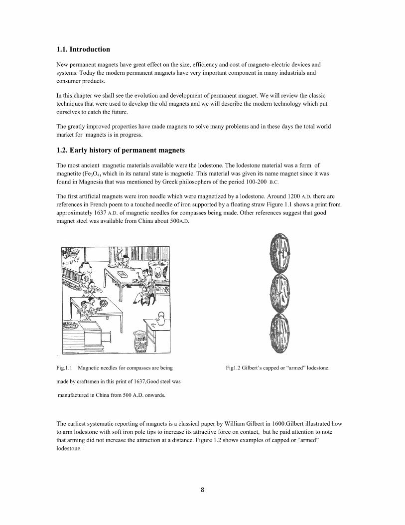
for uniformly magnetized cylinders. For material with high coercive force, or square loop demagnetization curves, the magnetization of simple geometries approaches the conditions of uniform magnetization at all points in the specimen. This leads to poles only at the terminals or end surfaces. Joseph’s data for cylindrical, rod shapes are shown in Figure 2.6. The factor N is plotted versus length to diameter ratio. Nb is the ballistic demagnetization factor to be used when the measurement involves the central or neutral cross-section of the cylinder. Nm is the magnetometric demagnetization factor to be used when the magnetic moment of the entire cylinder is involved.

Now we substitute (Bd + µoHd) for the magnetization Bi, we have an expression relating the induction Bd and the self demagnetizing field Hd to the magnet geometry and the factor N

By rearranging, the very useful load lone slope can be determined

Fig.1.9 Ballistic (Nb) and magnetometric (Nm) demagnetizing factors for cylindrical rods with invariant Bi.

In magnet design work, this ratio is used extensively. It is also referred to as unit permeance or the coefficient of self-demagnetization. Figure 2.7 shows the graphical relationships for high coercive force permanent magnet and the load line slope.

17

Fig.1.10 unit properties and the load line.

18

CHAPTER 2

CLASSIFICATIO OF PERMAET MAGETS

PROPERTY SYSTEMS AD MAGETISM PHYSICS

19

2.1. Classification of permanent magnets property systems

2.1.1. Introduction

In this chapter, magnets that are currently commercially important are described in terms of their composition, preparation, properties and the physical origin of their properties. Additionally, key processing and manufacturing issues are described. For reference, several older materials that may not be important commercially are also described because they bring out interesting examples of how the high properties are achieved. They add to the total body of information.

In general we find a sizeable number of different types in production at a given time. The design requirements are too diverse for one material to exclude all others. It is also true that once a permanent magnet material is made in production, it remains in production. This is undoubtedly due to the high cost of tooling magnetic devices and to the general sophistication of magnetic circuits. New improved properties are strong incentives to redesign and retool, but there is a reluctance to scarp what one knows has worked. For example, even some cobalt and tungsten steel magnets are still being used today.

2.1.2. Inclusion hardened magnets

Quench hardening steels were the first materials to be extensively used as permanent magnets. The development started with plain carbon steel and ended with the highly alloyed cobalt steels of Honda. They contain up to 1.25% carbon as a necessary constituent and generally have one or more of the following elements: manganese; chromium; tungsten; cobalt.

The origin of the coercive force in these quench hardened steels is due to the difficulty of domain boundary movement resulting from the combined effects of nonmagnetic inclusions, internal strains, lattice defects and sub-microscopic inhomogeneties in the material. The addition of cobalt raises the saturation magnetization, while the other elements mentioned lead to a decrease.

Conventional melting practice is used to prepare these magnet steels, which may be cast into final form or hot worked into bar and sheet stock and annealed. Magnet shapes may be hot formed at 900oC from annealed stock. The heat treatment for the magnets consists of heating to 800- 900oC and rapid oil or water quenching. The precise temperatures depend upon composition and are carefully controlled to obtain consistent magnetic properties.

A serious limitation of these steels with respect to permanent magnet use is the poor metallurgical stability at normal use temperature. By use of temperature cycling, the stability of these magnets was improved to the point of being tolerable for some uses. These magnets are rarely used today except in some hysteresis type applications Table 2.1 lists the typical properties of two, once popular, quench hardening steel magnet materials, 3.5% chrome and 36% cobalt. The demagnetization curves are shown in Figure 2.1.

20

Table 2.1 Properties of quench hardened magnets

Fig.2.1 Demagnetization curves of two martensitic steels.

2.1.3. Fine particles magnets utilizing shape anisotropy

2.1.3.1. Alnico magnets, Aluminium- ickel-Iron-Cobalt alloys

A major advance in permanent magnet use and technology was done by Mishima, with the discovery of the excellent magnetic properties of an aluminium-nickel-iron alloy. Many investigations added to Mishima’s work and many variations of composition, proceeding details and properties resulted. The single domain behaviour of these alloys is a result of the size and shape of the magnetic phase developed in weakly magnetic or nonmagnetic phase. The rapid development and success of these early isotropic Alnico1, 2, 3 and 4 are shown in Figure 2.2.

Fig2.2 Demagnetization curves of isotropic grades of Alnico.

21

The physical properties of Alnico alloys are rather poor. High coercivity is closely accompanied by extreme hardness and brittleness. Forming is by casting or sintering as close as possible to the desired size and shape. For close tolerances it is necessary to cut or wet grind the magnets.

Following the discovery by Mishima, and perhaps of greater importance, was the announcement by Jonas of a process to secure anisotropic feature: by cooling the magnet from an elevated temperature through the region of its curie point, under the influence of a magnetic field, it was found that a preferred axis of magnetization, parallel to the field axis, was developed in the magnet.

Alnico magnets are normally prepared in an induction melting furnace and the metal is poured into baked sand moulds. Small heats of 150-1000lb are generally used. Speed of melting and pouring is essential to prevent excessive oxidation losses and metal segregation. Figure 2.3 shows a block diagram of the process for making Alnico 5. The heat treatment is in three steps, a high temperature solution treatment followed by a controlled cooling in a magnetic and finally, a low temperature aging.

Fig. 2.3 Block diagram of process for Alnico 5.

The ability of the magnetic field to influence the geometry, and hence the anisotropy, of the decomposing phases lies in the mechanism of decomposition. The critical phenomenon in this process is the decomposition of the high temperature α-phase into the FeCo rich α-phase. This occurs by a spinodal decomposition mechanism. In a spinodal decomposition, a discrete precipitates does not form; rather, the two phases develop by gradual fluctuations in composition. The resulting structures are periodic and crystallographically oriented. Figure 2.4 illustrates how the process produces elongated regions of FeCo spaced in a lesser magnetic Fe-Ni-Al phase. Because the magnetic structure is influenced by crystallographic orientation during its formation, achieving the best properties requires careful development of the proper <100 > crystal texture. The sensitivity to crystal orientation is shown in Figure 2.5 for Alnico.

Fig.2.4 field orientation of Alnico 5.

22

Fig.2.5 Effect of crystal orientation on the magnetic properties of Alnico 5

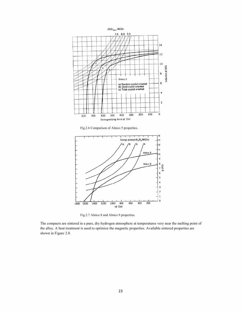
Alternately, random oriented casting may be recrystallized in a separate step. A continuous casting procedure reportedly also gave excellent crystal orientation. Property comparisons for Alnico 5 magnets are shown in Figure 2.6.

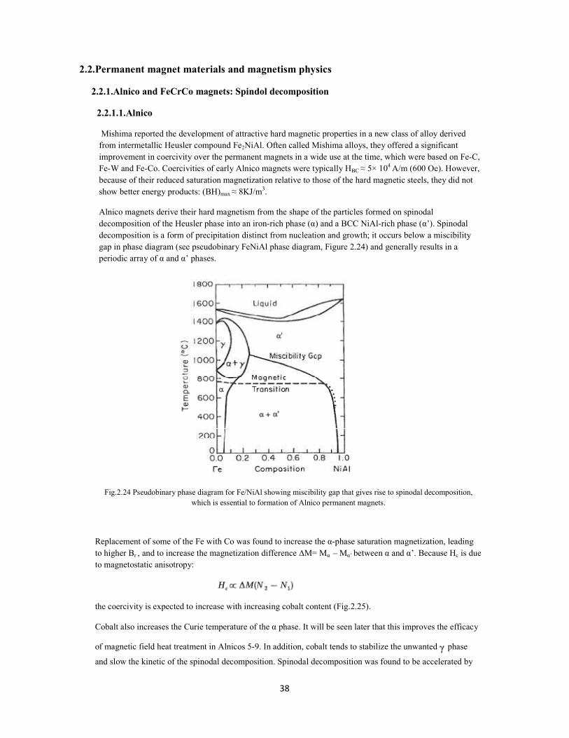
There are many compositional variations of Alnico magnets. Compositional changes to alter the shape and intercepts of the demagnetization curve or to improve the physical properties are extensive. A high titanium alloy, Alnico 8, and its directional grain counterpart, Alnico 9, are in extensive use. The unit magnetic properties are shown in Figure 2.7.

The difficulty in forming small magnets by casting, coupled with the poor physical properties led Howe to develop Alnico alloys made by powder metallurgy techniques. A mixture of the constituent metal powders and a lubricant are compacted in a forming die. Approximately 8% shrinkage occurs during sintering so this must be considered in the die design.

23

Fig.2.6 Comparison of Alnico 5 properties.

Fig.2.7 Alnico 8 and Alnico 9 properties.

The compacts are sintered in a pure, dry hydrogen atmosphere at temperatures very near the melting point of the alloy. A heat treatment is used to optimize the magnetic properties. Available sintered properties are shown in Figure 2.8.

24

Fig.2.8 Sintered Alnico 2, 5, 6 and 8.

Sintered Alnico magnets exhibit a uniformly fine grain, which greatly enhances the physical properties of these magnets. Sintered magnets are often required for high speed rotors in electrical machines. In the production of such rotors, it is common practice to allow the powder to shrink around a machinable steel insert which facilitates mounting the rotor magnet on a shaft. Complex small parts are readily produced to close tolerances.

2.1.3.2. Elongated single domain magnets

Elongated single domain magnets rely on shape anisotropy for coercivity. These magnets developed by General Electric are sold under the trade name Lodex. The sequence of processing steps is shown in Figure 2.9.Iron and cobalt are eletrodosited in mercury to form elongated structures and then subjected to the following processes: aging to remove the dendritic branches; addition of antimony to form a protective layer; addition of lead- antimony alloy to provide the metal matrix; pressing the slurry into a large block with field alignment; vacuum distillation to remove mercury; grinding to about 10µm powder and finally pressing at room temperature in a die in a field to the final shape. A series of unit property variations are obtained by varying the packing fraction of iron cobalt particles in the nonmagnetic alloy. Figure 2.10 shows the variations from this process for oriented magnets. Lodex magnets may also be extruded, in which case the orientation develops along the axis of extrusion. Lodex magnets find extensive use in small electromagnetic devices where close physical and magnetic tolerances are vital. Since the pressing is at room temperature, no shrinkage is encountered in this process.

25

Fig.2.9 Lodex process steps.

Fig.2.10 Anisotropic Lodex. From Hitachi magnetic corp.

2.1.3.3 Iron chrome cobalt magnets

Kaneko and his associates at Tohoku University announced the development of FeCrCo magnets. Properties vary much like those of Alnico5 and are obtainable with less cobalt and in ductile form. These magnets can be made by milling and casting, sintering or, as a wrought product in wire and sheet form. Fabrication by coining or stamping is also possible.

Typical heat treatment for FeCrCo is shown in Figure 2.11. A solution treatment is followed by a magnetic field treatment and finally, an aging treatment. At solution temperature, a body centred cubic phase (α) is formed. This phase is retained by quenching to room temperature. By reheating to 630oC the α-phase transforms into α1 and α2 phases. This part of the heat treatment is in a magnetic field which allows formation

26

of elongated particles in a direction parallel to the applied field. The aging treatment is used to increase coercive force by decreasing the magnetic properties of the α2 phase.

The process flow sheet for this alloy system is shown in Figure 2.12. Orientation by deformation has been described by Jim. The comparison of the two process approaches to alignment as a function of alloy percent Co is shown in Figure 2.13.

Fig.2.11 Heat treatment schedule for a FeCrCo alloy.

Fig.2.12 Process flow sheet, FeCrCo magnets.

27

Fig.2.13 Comparison of properties of magnets made by thermomagnetic treatment and by deformation alignment.

2.1.4. Fine particles magnets utilizing crystalline anisotropy

2.1.4.1. Ferrites

A new class of permanent magnetic materials was announced by Went, which was based on the crystal anisotropy of barium oxide. This class of magnets is generally known as ferrite, but are sometimes referred to as oxide or ceramic magnets. Today, ferrite magnets are by far the most widely used magnets. The success of ferrite is due to several reasons. The raw materials are inexpensive and non strategic. The high coercive force combined with reasonable induction has allowed permanent magnets to move into many types of small motors.

Ferrites are produced by powder metallurgy. Their chemical formulation may be expressed as MO.6(Fe2O3) where M is Ba, Sr, or Pb. Strontium ferrite has higher coercive force than barium ferrite and is the larger production ferrite. Lead and barium ferrite both have some production disadvantage from an environmental point of view. Table 2.2 shows the range of properties available.

Table 2.2 commercially available ferrite properties.

Ferrite magnets are available in isotropic and anisotropic grades. Figure 2.14 shows the steps used in preparing barium ferrite. The anisotropic grades are prepared by pre-firing the raw materials and milling the compound to single crystals of the order of single domain size ( about 1µm). The milled powder is then wet or dry pressed under the influences of a magnetic field. The pressed compacts are then sintered in air. The shrinkage is about 15% and ferrite magnets must be ground to maintain close tolerance parts. The ferrite

28

particles develop as platelets with the preferred C-axis of magnetization perpendicular to the plane of the plate. Pressing promotes mechanical anisotropy and somewhat better properties are achieved in the pressing direction than in a transverse direction. In making the oriented magnet, the field should be applied in the direction of pressing. A field of 5KOe is required to produce oriented magnets. Wet pressing gives the particles increased mobility and improved Br and (BH)max . Dry pressing, however, is faster since the water does not have to be removed during the pressing. Figure 2.15 shows a general flow chart of the ferrite production process.

Fig.2.14 Steps used in preparing barium ferrite.

By combinations of pre-firing time and sintering temperatures, a wide range of properties can be obtained. Also, grain growth inhibitors may be added to influence Br/Hci relationships. Figure 2.16 gives summary of progress in property development with respect to time. In each time frame, the points represent commercially available properties with trade-offs between Br and Hci.

The saturation magnetization of a ferrite single crystal is approximately 5KG. Hci measurements on single particles have been reported as high as 11.3KOe. One can only expect small improvements in Br since we are already close to the limits imposed by the saturation magnetization.

29

Fig.2.15 Ferrite magnet production process.

Fig.2.16 Ferrite property development trends.

30

2.1.4.2 Manganese-Aluminium-Carbon system

Koch developed the first anisotropic alloy in this system. Properties as high as (BH)max = 3.5 MGOe were obtained as a result of cold working by swaging. The extreme brittleness and difficulties in swaging limited the usefulness of these magnets. Kubo found that the addition of carbon to the MnAl alloy improved the stability of the meta-stable ferromagnetic phases and also improved the coercive force. Kubo later clarified the nature of the crystallographic transformation process which resulted in a new process for making MnAlC magnets. From a detailed study of applying pressure in various directions, it was learned that crystal structure could be formed presumably by an alignment effect of atoms due to external stress. The direction of the C axis of the ferromagnetic phase was changed and a hot plastic deformation process led to the formation of highly anisotropic magnets. Figure 2.17 shows the improvement in alignment by extrusion.

Fig. 2.17 MnALC property improvement due to extrusion.

Matsushita Electric Co. has produced properties of Br = 5500 G, Hci = 3000Oe and (BH)m = 7.5 MGOe. The nominal composition is 70Mn, 28.5 Al, 0.8 Ni and 0.5 C. Unfortunately it has a low curie temperature and hence a high reversible temperature coefficient (0.12% /oC). Additionally, its coercive force drops rapidly with increasing temperature. It would seem that MnAlC magnets are limited to applications in which the maximum temperature is not over 100oC. An advantage is that the material is machinable. However, the high investment in deformation equipment for orientation is a serious drawback.

2.1.4.3. Platinum Cobalt

This alloy has very unique properties, but its high cost limits its use. The best properties are obtained in the 50:50 atomic ratio. A 10 MGOe material is obtained with the following thermal events. Heat to 1000oC to yield a disordered structure, cool at a controlled rate to room temperature, and finally, age at 600oC for 5 h. The high Hci may be attributed to the high crystal anisotropy of tetragonal single domain regions. PtCo is isotropic, it has a high ratio of Br/Bis (0.86) which suggests that the final partially ordered material has cubic magnetocrystalline anisotropy.

31

2.1.4.4. Rare-earth cobalt magnets

Early processing approaches to make rare-earth cobalt magnets were quite varied. Important characterization and measurements of saturation magnetisation and anisotropy fields of powder, as well as projection of the permanent magnet potential of many rare-earth cobalt compounds was done by Strnat and Hoffer.

The making of real magnets was a long and difficult development. A densified magnet having 20 MGOe properties was reported by Buschow. The densification process involved a combination of isostatic and uniaxial pressure of about 20Kbar. Martin and Benz described the use of liquid phase sintering to produce SmCo5 magnets with excellent magnetic properties and high physical density. The processing involved vacuum melting of Sm and Co. The flow chart of the process is shown in Figure 2.18. The earliest SmCo5 magnets were aligned in a high magnetic field and then hydropressed and sintered. Later developments led to die pressing in a magnetic field of about 10KOe. Die pressing has proven to be a satisfactory compromise between property achievement and processing cost.

Fig.2.18 SmCo5 production process

Cech developed a reduction diffusion process that allowed Sm-oxide powder and cobalt powder to be reduced with Ca to form the compound directly without the need to start with pure Sm metal. This process (Figure 2.19) and a similar processes had a profound economic impact on the development of rare-earth cobalt magnet industry. Since Sm oxide costs considerably less than pure Sm metal. The SmCo5 process has, over the years, been modified to reduce the Sm content. Ce misch-metal, being of less cost than Sm, has been used extensively. Up to half of the Sm was replaced and properties of about 14MGOe were achieved. Pr has also been substituted for Sm to improve properties. Property levels of 26 MGOe have been achieved.

A totally different processing approach to rare-earth cobalt magnets was announced almost simultaneously by Nesbitt and Tawara. They achieved very high coercivity in bulk SmCo and CeCo alloys in which a two phase microstructure was created by substituting Cu for part of the Co. This was a precipitation type cast structure with properties as high as 8.0 MGOe reported. A later development direction was to use powder metallurgy methods, including sintering to make useful permanent magnets. The five element system Ce Sm (Co Fe Cu) has many variations of properties and these magnets are often preferred over SmCo5 due to improved cost/performance, particularly in the Japanese market. However, the properties do not allow substitution for SmCo5 in some situations.

32

Fig.2.19 reduction/ diffusion process.

An important class of rare-earth cobalt permanent magnet has the general composition R(Co, M)z where R stands for at least one rare-earth element, M for a combination of transition metals and /or copper and z is between 6 and 8.5. These multicomponent magnet alloys are generally termed the 2:17 system. They have the advantage of higher magnetization and use less Sm and Co. The processing steps are very similar to those of SmCo5, except the heat treatment is longer and may involve step aging. In early investigations of these compounds, Strnat found that generally, the 2:17 compounds had an easy plane of magnetization and only SmCo17 had easy axis magnetization necessary for coercivity. By replacing some of the cobalt with iron, the anisotropy field was increased to useful levels. Additional improvements in this system came from adding small amounts of Cr, Mn, Ti, Hf and Zr. Michra described a 30 MGOe magnet having an Hci of 13KOe with a composition Sm( Co0.63Fe0.28Cu0.05Zr0.02)7.7. The commercial properties available generally involve two distinct levels of coercive force. For low values of z, Hci is about 6KOe and for higher z values with higher Fe content Hci levels of 12.5KOe are offered. In these materials the coercive force mechanism is domain wall pinning at grain boundaries.

Table 2.3 shows the typical unit properties available for the now numerous types of rare-earth cobalt magnets, in addition to rare-earth iron properties.

33

Table 2.3 Magnetic properties chemical composition of rare-earth magnets.

2.1.4.5. dFeB (Sintered)

In Japan was announced the development of a new rare-earth iron permanent magnet having a (BH)max of 35 MGOe. Sagawa later described compositional and processing details. The new magnet involved essentially the same powdered metallurgy approach as used for making SmCo5. During the past years there has been a tremendous development effort on sintered NdFeB magnets. Today a wide variety of commercial magnets are offered with properties from 27-35 MGOe. Some producers offer a “H” grade in which compositional additions to the normal NdFeB magnet have been made to enhance Hci and hence improve the high temperature stability.

The process flow chart is very similar to that outlined for SmCo5. Again there are two routes to alloy preparation. Either the vacuum melting of the elements or the caciothermic oxide reduction process can be used. Table 2.4 shows an interesting comparison between sintered rare-earth cobalt and sintered rare-earth iron magnets. The mechanical properties of NdFeB are superior to those of SmCo5. The principal disadvantage of NdFeB is the large change in magnetic properties with temperature.

34

Table 2.4 Comparison of the magnetic and physical properties of NdFeB and SmCo magnets.

2.1.4.6. dFeB (melt spun)

Croat described work at General Motors on the melt spinning approach to making a rare-earth iron magnet. Isotropic properties of 14 MGOe were achieved. Somewhat later Lee described a hot deformation technique for orientation of the melt spun material giving anisotropic properties of 40 MGOe. The alloy is quenched rapidly and a ribbon is formed with a very fine microcrystalline structure having high crystalline anisotropy. By control of the solidification rate the microstructure is optimized. The NdFeB melt is under an argon atmosphere. The ribbon fragments from the wheel are the basic building blocks for several unit property demagnetization characteristics having different physical and magnetic parameters. General Motors calls this process Magnequench. The process flow chart and the end processing variations leading to MQ I, MQ II and MQ III grades are shown in Figure 2.20. MQ I is a matrix or bonded version and is isotropic. MQ II is a fully dense magnet achieved by hot pressing and is also isotropic. MQ III magnets are anisotropic and are made by taking the fully dense, hot MQ II magnet and hot deforming the magnet so that its area is increased and its dimension parallel to pressing is decreased. This hot deformation involves a transverse plastic flow. The magnequench crushed ribbon is relatively large (200µm) and can be exposed to air without appreciable oxidation. This new processing approach moves magnet making from the traditional batch processing approach toward the automated factory with major advantage such as improved quality, cost effectiveness and versatility. This forming approach opens the way for making integrated permanent magnet circuits. For example, iron powder and magnet material may be pressed together in one die system to form magnet and return path circuit.

35

Fig.2.20Magnequench process.

2.1.5. Matrix or bonded magnets

A major class of permanent magnets has evolved from ferrite and rare-earth powders imbedded in rubber, resins and plastics. Depending on the magnetic material loading these products may either be flexible or of rigid form. These permanent magnets are offered in a wide range of properties from 0.5 to near 20 MGOe. They may be formed by rolling, extrusion, compression and injection moulding. The magnet components can be formed in complex shapes with close mechanical tolerances. Bonded magnets, of course have lower levels of B compared to their fully densidied counter parts. Both isotropic and anisotropic products are offered. The ferrite bonded magnets have good high temperature stability, but stability is a problem in the rare-earth bonded magnets. The best stability is achieved with metal bonded magnets described by Strnaut. Resin bonded magnets are limited to approximately 100oC at this time.

Magnequench powders are also being in injection moulded magnets products with 6MGOe isotropic properties attainable. Magnequench MQ III powders have recently been made into bonded magnets exhibiting properties up to 16 MGOe with Hci levels of 17 KOe. The coercive force levels were achieved with Ga additive (NdFeGaB). The stability of these magnets appears to be excellent up to 150oC.

2.1.6. Semi-Hard magnets (Hysteresis alloys)

Several permanent magnet materials that were described , find wide use in hysteresis motors, brakes and torque drives. The maximum torque which a hysteresis device can develop is a function of Eh, loss per cycle or the area of the hysteresis loop of the rotating material. There are actually two fundamentally different hysteresis effects. We tend to be most familiar with alternating hysteresis in which B and H vectors are parallel in space and the magnitude of H is changed. The other type of hysteresis loss involves rotating a volume of magnetic material in a field of constant magnitude, but varying in direction. This is known as rotational hysteresis loss. Figure 2.21 illustrates domain wall movement in each hysteresis relationship. In some hysteresis devices the loss and torque developed is largely due to rotational effect, while in others both effects are present. Figure 2.22 shows how each effect changes with material flux density B. The convenient way to measure rotational hysteresis loss is to draw torque curves using a torque magnetometer. A torque curve is drawn and then redrawn, turning the specimen in the opposite direction. The two curves will be displaced relative to each other and the area between them will be proportional to the rotational influence, hysteresis devices tend to be analysed and property comparison made on the basis of alternating hysteresis.

36

Fig.2.21 Domain wall motion in hysteresis devices.

Fig.2.22 hysteresis relationships.

A general figure of merit for a hysteresis device is the ratio Eh/Hp where Hp is the peak magnetizing force developed in the device. Figure 2.23 compares several materials by plotting Eh as a function of Hp. A dot on each curve indicates the most efficient operating point in terms of maximizing Eh/Hp. Due to the complex relationships involving hysteresis loss, field magnitude and field direction selecting properties and optimizing, hysteresis devices tends to be a rather empirical process.

37

Fig.2.23 alternating hysteresis losses versus magnetizing force.

38

2.2.Permanent magnet materials and magnetism physics

2.2.1.Alnico and FeCrCo magnets: Spindol decomposition

2.2.1.1.Alnico

Mishima reported the development of attractive hard magnetic properties in a new class of alloy derived from intermetallic Heusler compound Fe2NiAl. Often called Mishima alloys, they offered a significant improvement in coercivity over the permanent magnets in a wide use at the time, which were based on Fe-C, Fe-W and Fe-Co. Coercivities of early Alnico magnets were typically HBC ≈ 5× 104 A/m (600 Oe). However, because of their reduced saturation magnetization relative to those of the hard magnetic steels, they did not show better energy products: (BH)max ≈ 8KJ/m3.

Alnico magnets derive their hard magnetism from the shape of the particles formed on spinodal decomposition of the Heusler phase into an iron-rich phase (α) and a BCC NiAl-rich phase (α’). Spinodal decomposition is a form of precipitation distinct from nucleation and growth; it occurs below a miscibility gap in phase diagram (see pseudobinary FeNiAl phase diagram, Figure 2.24) and generally results in a periodic array of α and α’ phases.

Fig.2.24 Pseudobinary phase diagram for Fe/NiAl showing miscibility gap that gives rise to spinodal decomposition, which is essential to formation of Alnico permanent magnets.

Replacement of some of the Fe with Co was found to increase the α-phase saturation magnetization, leading to higher Br , and to increase the magnetization difference ∆M= Mα – Mα’ between α and α’. Because Hc is due to magnetostatic anisotropy:

the coercivity is expected to increase with increasing cobalt content (Fig.2.25).

Cobalt also increases the Curie temperature of the α phase. It will be seen later that this improves the efficacy

of magnetic field heat treatment in Alnicos 5-9. In addition, cobalt tends to stabilize the unwanted ᵧ phase

and slow the kinetic of the spinodal decomposition. Spinodal decomposition was found to be accelerated by

39

the addition of up to 3.5% Cu and by reduction of the Ni and Al content. Finally, the addition of up to 4 or 5% Ti helps offset the deleterious effects of cobalt; while it lowers Br , the increase it brings to HBC is enough to increase (BH)max.

Fig.2.25 Variation of remanence, coercivity and maximum energy product with cobalt substitution for iron in FexCo1-xNiAl.

Anisotropic Alnicos A thermomagnetic treatment for the development of anisotropic Alnicos (those designed as Alnicos 5-9) was discovered early.

The idea is to establish an energetic preference for particle elongation along the ˂ 100 > direction closest to an applied field. The internal magnetic field near α- α’ interface is proportional to the surface magnetic charge

density resulting from a difference in perpendicular magnetization across the interface, Hi α ∆M = Mα- Mα’. The two phases are characterised by magnetization thickness products Mαtα and Mα’tα’. The magnetostatic contribution to the surface energy then goes as σm ≈ (µ0/2) ∆M ˂ M > (tα+ tα’) cos2Ѳ, where ˂ M > = (Mαtα.t)/ (tα + tα’) is the thickness averaged magnetization. Here Ѳ is the angle between the magnetization direction and the normal to the interface, which is assumed here to be planar. For the interface energy averaged over a magnetized particle, the factor cos2Ѳ is replaced by an effective demagnetization factor. For µ0∆M ≈ µ0 (M1- M2) ≈ 0.1 T, at the initial stages of spinodal decompositions, the surface energy can be estimated to be σm ≤ 0.4 mJ/m2 for 0.1 µm particles characterized by a demagnetization factor N ≈ 0.1. This magnetic contribution is significant compared to typical chemical interface energies (which are of order 1 mJ/m2).

Interfaces that are parallel to the magnetization direction (Ѳ = 90o) have zero magnetostatic energy (Fig.2.26a) and the magnetostatic energy is less than that for a sharp interface.

Fig.2.26 Schematic representation of the effects of magnetization on interfacial energy. (a) Magnetization parallel to an interface produces no surface magnetic charge; (b) perpendicular magnetization discontinuity across an interface results in a charged surface and generates magnetostatic fields that raise the energy; (c) a diffuse interface distributes the magnetic charge and reduces the magnetostatic energy.

40

Whereas the nonmagnetic interface energy ᵧA tends to favour spherical particles (A is the surface area of the

particle and ᵧ is the Gyromagnetic ratio), the magnetostatic energy fmsV is the driving force for particle

elongation (f is Helmholtz free energy per unit volume and V is the particle volume), and fmsV ≈ µ0MS2∆NV is

a measure of the extensive magnetostatic energy saved by elongation. The energy reduction is proportional to the change in demagnetization factor ∆N during growth. If the particle grows elongated in its direction of magnetization, then its magnetostatic energy is reduced from that of a sphere to a smaller value characteristic of its elongated shape. The rate of elongation is therefore proportional to

Larger particles (smaller surface: volume ratio) are more strongly driven to large aspect ratios. To develop long particles while they are still small enough to display single domain behaviour, it is helpful to maximize fms by using as much cobalt as possible; this increases Tc and ∆M..

Optimal parameters for Alnico 5 are (BH)max = 10.8KJ/m3 perpendicular to the texture and 13.4KJ/m3 parallel to the texture. Increasing cobalt content has stronger benefits for anisotropic Alnicos; for 23% Co (BH)max = 41.6KJ/m3 can be achieved .

Even though a particular direction for α elongation is established by the field applied during decomposition and tempering, there remains in polycrystalline samples a dispersion in the orientation of ˂ 100 > directions and hence the texture is not optimized. It was found that the properties of anisotropic Alnico could be enhanced by increasing texture in the microstructure. This could be accomplished by chilling the end faces of the casting mould to promote directional solidification.

Figure2.27 shows the second quadrant B-H curves for anisotropic Alnicos 5-9 (a directed- growth variation of Alnico8), as well as for single-crystal Alnico 5 (dotted). Table 2.5 summarizes the compositions and properties of the data in Figure2.27. Note the dramatic improvement in magnetic properties, particularly (BH)max, that comes with grain alignment by directional growth (DG) and development of single crystal Alnico 5 (dotted line). Alnico 9 achieves its higher coercivity with greater cobalt content remanence, has in DG form an energy product comparable to that of single crystal Alnico 5.

Fig.2.27Second-quadrant B-H curves for selected anisotropic Alnicos; maximum BH products can be determined from the dashed BH constant hyperbolas.

41

Table 2.5 Compositions and magnetic properties of Anisotropic, thermomagnetically treated Alnico 5 and 8 as well as single crystal Alnico 5.

With the development of highly textured α- α’ phase separation in the Alnico, it is possible to attempt to describe the magnetic behaviour in terms of the Stoner-Wohlfarth model for single-domain, anisotropic particles.

Typical α-FeCo particles in Alnico 5 measure 1500Ǻ long by 400 Ǻ in diameter. The shape anisotropy of such particles is related to the following equation:

The magnetostatic energy is the energy of the average magnetization ˂ M > in the field from the magnetization discontinuity at the interface, ∆M. For simplicity, choose Mα = 3Mα’ = 2.1 T/µo so that ˂ M > ≈ ∆Ms ≈ 1.4T/µo . ∆N = Nl - Nll can be calculated from the previous equations, for prolate spheroids with m ≈ 4. These numbers give Ku ≈ 1.1 × 105 J/m3 and thus Ha ≈ 1.8 × 105 A/m . Nesbitt and Williams used torque magnetometry to determine the strength of the uniaxial anisotropy of Alnico 5 to be 105 J/m3, where (Ku is uniaxial magnetic anisotropy energy coefficient, m is mass, H is magnetic field intensity and N is number of particles).

Figures2.28.a and 2.28b compare the measured orientation dependence of Hc with the calculations of Shtrikman and Treves using the curling form of the SW model. The rough similarity in the shape of the experimental and calculated curves for large S values suggest that many particles exceed the single domain size for this composition: S = r/ro >> 1 with ro = (4ᴨA/µo )

½ /Ms, where A = surface area of the particle.

Fig2.28 (a) Dependence of the coercivity on the angle Ѳ between the preferred axis and the measurement direction measured after saturation Hc and from remanence Hr for anisotropic Alnico 9 (A) and for single crystal Alnico 9 (T); (b) reduced coercivity versus Ѳ calculated for single domain particles of various effective radii S.

42

2.2.1.2. Fe-Cr-Co

BCC Fe-Cr-Co alloys develop hard magnetic characteristics by spinodal decomposition as do the Alnicos. However, the product phases in Fe-Cr-Co are relatively ductile Fe-rich (α) and Cr-rich (α’) phases compared to FeCo and NiAl. Magnetic properties of Fe-Cr-Co magnets can be enhanced by field-annealing to introduce an elongated morphology (small Mo additions help here) and low temperature tempering to enhance the α - α’ phase separation. Coercivities of 65KA/m and energy products approaching 80 KJ/m3 have been achieved.

Ductility is a major reason for the interest in Fe-Cr-Co magnets; it allows a certain amount of machining on parts, and it has been exploited by using uniaxial deformation to enhance alignment and thus increase Hc and the energy product. The low cobalt content of this family of magnets is also of commercial interest.

One would expect the properties of Fe-Cr-Co to be optimized when Mα – Mα’ is maximized (nonmagnetic Cr- rich phase).

Two permanent magnets based on FCC spinodal decomposition are known to exist: Cu-Ni-Fe (Cunife) and

Cu-Ni-Co (Cunico). In both cases the Cu-poor phase (ᵧ) is strongly magnetic while the Cu-rich phase (ᵧ’) is

nonmagnetic. The very good ductility of these alloys allows strong texture to be developed by uniaxial deformation.

2.2.2. Rare earth transition metal intermetallics

Hard magnets based on SmCo5 boast the highest uniaxial anisotropies of any class of magnet, Ku ≈ 107 J/m3. On the other hand, phases based on Sm2Co17 exhibit higher flux density and Curies temperature. The more recently developed magnets based on Fe14Nd2B exhibit the highest energy products achieved so far in permanent magnets.

1- The variation across the lanthanide series of the quantum numbers, the calculated effective moments gµB J(J+1)½

, saturation moment µm = gµBmj, and the observed moments are shown in Table2.6. Except for Gd, the R species are characterized by L≥S. Hund’s third rule states that L and S combine subtractively in the first half on the 4f series. For light R species the net moment is reduced and is antiparallel to L (because negative electronic charge makes µB ˂ 0). L and S combine additively in the second half of the series, so there the net moment is enhanced and is antiparallel to both L and S. The effective magnetic moments of the heavy R species reach a higher maximum value than do those of the light R species. The ordering temperatures are low or negative for the light R elements; these materials show spiral or canted spin structures rather than ferromagnetism. Figure2.29 shows the variation of the measured effective moment and the magnetic ordering temperatures across the rare-earth metal series. The variation of the rare-earth moments across the series is fairly well described by the quantum numbers in Table 2.6. The variation of the magnetic ordering temperatures is systematic in the heavy R metals, as will be described below.

2- The Curie temperatures of the rare-earth metals and of various rare-earth alloys vary in asystematic way with the de Gennes factor, G = (g-1)2J(J+1) as shown in Figure2.30. The de Gennes factor has its basis in the molecular field expression for the Curie temperature which is proportional to S(S+1); the term (g-1)2 in the de Gennes factor singles out the spin (g =2) part of the moment from J(J+1). Thus the Curie or Nèel temperatures scale with the spin part of the magnetic moment, as well as the square of the total angular momentum. The variation of the Curie temperature with R species for the Co5R, Co17R2, Fe14R2B and R2Fe17 intermetallic series are shown in Figure2.31. The variation of Tc with R species in the two iron-based series is well described by the effective spin or de Gennes factor, G = (g-1)2J(J+1), which decreases on either side of Gd in the series. Another remarkable feature of this figure is the general decrease in Tc as Fe concentration in the compounds.

43

Table 2.6 Electronic structure as well as the calculated and experimental values of the effective and saturation magnetic moment in Bohr magnetons for rare-earth ions and metals.

Where (S is spin quantum number of atom, quantum number, J is total angular momentum, g is gibbs free energy per unit volume and µBBohr magneton).

Fig.2.29 Above, variation of the Hund effective moment and the moments observed for +3 ions and metals of the rare-earth (R)

series; below variation of magnetic ordering temperatures for R metals.

44

3- For rare earth transition metal (R-TM) intermetallics, it is important to understand the nature of the coupling

between the rare-earth moment (µR = gµBmj ) and that of the transition metal species ( µTM = gµBms), where (mj is quantum number for the z component of total angular momentum and ms is quantum number for the z component spin angular momentum). The magnetic moments of transition metals are observed to couple ferromagnetically with light rare-earth moments (J.s > 0) and antiferromagnetically with heavy rare-earth moments (J.s ˂ 0). Recall that in the first half of a shell, J = L – S (total moment and spin moment are antiparallel) and in the second half. J = L+S. The spin- spin coupling between R and TM species is always antiferromagnetic. It has been suggested that R-TM coupling is due to the antiferromagnetic conduction-electron-mediated exchange as described by the RKKY model. However, the applicability of the RKKY model to this problem is questionable because variations in R-TM separation do not change the sign of the coupling.

Fig.2.30 Dependence of magnetic transition temperatures of R metals and R-R alloys on the de Gennes factor,

G = (g-1)2J(J + 1)

Fig. 2.31 Variation of the Curie temperature with R species in four series of R-TM intermetallics of importance as permanent

magnets.

4- Finally, for permanent magnet applications, it is important that the crystal system be uniaxial rather than cubic and that the anisotropy gives rise to an easy axis (Ku > 0) as opposed to an easy plane (Ku ˂ 0). The latter leads to easy

45

demagnetization and low coercivity because the sample can demagnetize without M rotating to a hard direction. The rare-earth metals show complex spiral spin structures in many cases as well as easy-axis magnetization (Gd from 240 to 293 K), and easy magnetization (Gd from 170 to 220 K or Tb and Dy up to 222 and 83 K, respectively). Thus it is not surprising that their intermetallic alloys also show a rich variety of spin structures. This important effect limits the range of alloy substitutions available in designing new R-TM permanent magnets. For most of the RCo5 intermetallics with light R species (R = Y, La, Ce, Pr, Nd, Sm), k1 > 0. The situation is more complex in the R2Co17 and in the Fe14R2B .

2.2.3. Cobalt-rare-earth magnets

CoR magnets are based mainly on the two phases R2Co5 and R2Co17. Although the first structure is more widely known, most CoR magnets are , in fact, multiple composites of these two structures and sometimes other phases. The Co-Sm phase diagram is shown in Figure2.32 Co5Sm is stable only above 850oC. Thus, its use is limited to temperatures below which kinetics preclude transformation to the more stable Sm2Co7, Sm2Co17 and Co phases. The R species form hexagonal nets with a smaller Co hexagon in the same plane and similar hexagonal Co layers ( rotated by ± 30o) are stacked between the R nets.

Fig.2.32 Equilibrium phase diagram for SmCo near the cobalt rich limit.

This uniaxial structure together with the orbit angular moment of the R species is the source of the magnetocrystalline anisotropy of the RCo5 system. SmCo5 exhibits a magnetocrystalline anisotropy of 107 J/m3. Fig 2.33 shows the easy and hard axis magnetization curves for the two principal Co-Sm magnets an Fe14Nd2B. Single phase SmCo5 can exhibit room temperature intrinsic coercivities, Hjc of 3.2 MA/m (40 KOe) and maximum energy products of over 200 KJ/m3 (24MG.Oe). This, combined with their relatively high Curie point ( Tc = 685oC), makes them suitable for a wide range of applications. Iron substitutions for cobalt lead to a change from easy axis magnetization to easy plane magnetization in RCo5. Because of the large magnetic anisotropy of SmCo5, a 180o Bloch wall in this material should have a width of only 3.1 nm. Further, the domain wall energy density is 40 mJ/m2 , 100 times that of a soft material. It is not surprising, therefore, that the magnetization process in single phase RCo5 intermetallics is limited by reversal domain nucleation. Once nucleation occurs, domain walls move relatively easily until they reach again boundary, as in Ba ferrites. Hence, initial efforts to produce cobalt/rare-earth magnets focused on the fabrication of single-domain SmCo5 particles. It was discovered by

46

Nesbitt that small substitutions of Cu for Co would lead to the precipitation of a nonmagnetic phase which increased the coercivity. They showed that the heat treatment of R(CoCu)5 magnets results in precipitation of a dispersion of fine ( d ≈ 10nm) second phase, Cu rich particles in a R2Co17 matrix having a grain size of order 10 µm. The coercivity mechanism becomes domain wall pinning on the small nonmagnetic SmCu5 particles.

Fig.2.33 Easy-axis and hard-axis magnetization curves for RCo 1-5 and 2-17 compounds.

Tawara and Strnat showed that magnetic hardening by Cu precipitates could be extended in Sm(CoCu)x from x = 5 to x ≈ 7.2. Further extension to x ≈ 8.5 by inclusion of other transition elements led to the first practical R2TM17

magnets. These structures have the same cobalt hexagonal nets that occur in the RCo5 compounds but fewer R atoms in the adjacent layers. Whereas R atoms are located at the centres of alternate hexagonal Co rings of the 1-5 compound, a TM atom occupies an axial site in the midplanes between certain of these hexagonal rings (Fig.2.34). The magnetocrystalline anisotropies of R2Co17 phases ( 3-4 × 106 J/m3) are generally less than those of the corresponding 1-5 phases (11- 20 × 106 J/m3), but the 2-17 saturation magnetizations and Curie temperatures are generally greater (see table 2.7). The rhombohedral crystal structure of the 2-17 compounds allows incorporation of greater Fe content than does the 1-5 hexagonal structure. Coercivities of order 800 KA/m (10KOe) and energy products of order 240 KJ/m3

have been reported in single phase Sm2(CoFe)17 based alloys. Because the rhombohedral 2-17 phase has a lower anisotropy than the 1-5 phase, heat treatment and inclusion of nonmagnetic atoms to promote optimal phase segregation are generally used to achieve higher coercivities. The Curie point and saturation flux density are substantially improved by partial Fe, Zr and Cu substitutions for Co. These substitutions also promote formation of a cellular microstructure based on a 2-17 rhombohedral phase, a 1-5 intergranular phase and a Zr rich platelet phase . This cellular microstructure provides the pinning sites needed to obstruct domain wall motion in 2-17 magnets. In contrast, high coercivity in the 1-5 magnets is a result of inhibited nucleation. The cellular microstructure of 2-17 magnets is generally sensitive to heat treatments; the maximum use temperature is limited to about 300oC. However, 2-17 permanent magnets of the modified composition Sm2(CoFeZrCu)17 are attractive for high temperature applications because of their high values of the ferromagnetic Curie point ( Tc = 810oC) , saturation magnetization (µoMo = 1.5 T) and at 25oC (BH)max = 24-30 MG.Oe. A further advantage of this two phase, 2-17 system when it incorporates a significant fraction of iron is reduced cost relative to Sm2Co17. Single phase TbCu7 type thin film magnets of Sm(CoFeCuZr) compositions can be sputter deposited to exhibit either high intrinsic coercivities or as aligned films, to exhibit enhanced energy products. Coercivity in excess of 16KOe at room temperature has been observed in fields of ± 18 KOe in single phase TbCu7 type films crystallized from amorphous deposits. Relatively thick sputtered films exhibit strong in plane c-axis alignment for a wide range of film thicknesses up to 120µm. An important feature of these in plane c-axis TbCu7 type film is that their magnetic properties appear to be insensitive to thermal treatments up to nearly 500oC.

47

Table 2.7 compares some room temperature properties of Co5Sm and Co2Sm17 magnets with those of the Fe14Nd2B class. Figure2.35describes the change in preferred magnetization direction from easy axis to easy plane as various transition metals are substituted for Co in R2Co17 magnets.

Fig.2.34 Rhombohedral, Th2Zn17 type crystal structure on which R2Co17 magnets are based.

Table 2.7 Comparison of some Magnetic properties for SmCo5, Sm2(CoFe)17 and Fe14Nd2B permanent magnets at 25oC.

48

Fig.2.35 Influence of transition metal substitutions on the anisotropy (magnetic symmetry) of R2Co17.

The 2-17 magnets are used in multiphase form to enhance coercivity by domain wall pinning. Without domain wall pinning, the coercivity would be relatively small. On the other hand, the stronger anisotropy of RCo5 magnets makes nucleation limited coercivity viable. Nucleation limited coercivity would not be strong enough in a single phase 2-17 magnet because of its larger magnetization and smaller anisotropy relative to SmCo5 . Due to the larger concentration of Co in even the two phase Co-R magnets, their cost per Kiloguass of saturation flux density remains very high. This provided the impetus for development of less expensive high energy magnets based on iron. Rare-earth intermetallics based on Fe14d2B1

Fe-Nd-B magnets represent an important class of rare-earth intermetallic compounds that advance the technology of permanent magnets beyond that of the Co-R magnets. Their development came as a result of the cost and limited world supply of cobalt. The attractive permanent magnet properties of Fe14Nd2B1 magnets arise from several factors:

1. The large uniaxial magnetic anisotropy ( Ku = +5 × 106 J/m3) of this tetragonal phase. 2. The large magnetization ( Bs= 1.6 T) owing to the ferromagnetic coupling between the Fe and Nd moments. 3. The stability of the 14-2-1 phase, which allows development of a composite microstructure characterized by 14-2-

1 grains separated by nonmagnetic B-rich and Nd-rich phases, which tend to decouple the magnetic grains. The tetragonal Fe14Nd2B1 structure (Fig.2.36) contains four formula units and has unit cell dimension of a = 0.88nm and c = 1.22nm. There are six distinct Fe sites, two distinct Nd sites, and one B site. The unit cell consists of eight layers vertically stacked. All the Nd and B sites are found in layers at z = 0 and ½. Most of the Fe atoms reside in puckered hexagonal nets between the Nd and B rich layers. The Fe net puckering is associated with an attractive Fe-B bonding that places the B at the centre of trigonal prism of Fe(e) and Fe(K) atoms. The Fe(j) sites are the most highly coordinated by transition metal atoms and not surprising, show the largest magnetic moments. The 14-2-1 unit cell shows the usual lanthanide contraction when Nd is replaced by other R species. The saturation magnetization versus temperature of the Fe14R2B series is shown in Figure2.37. The data are separated into two groups, the light rare-earth and the heavy rare-earth species. The Ms(T) behaviour in the former

49

appears to have the normal shape of a Brillouin function. In contrast, the Ms(T) behaviour of the late R species resembles the M(T) form characteristic of ferrimagnets for which the magnetization of the higher Tc sublattice (Fe in this case) is greater than that of the lower Tc sublattice(R). Thus, there are no compensation temperatures in the Fe14R2B1 series. To interpret these data, recall first that the magnetic moments of the six iron sites (averaging 2.1 µB/Fe) are ferromagnetically coupled to each other. Figure2.37 then suggests a ferromagnetic coupling of the net TM moment to the R moment in the first half-series and an antiferromagnetic coupling in the second half-series. The same was found to be true of CoR intermetallics and it is generally the case for other rare-earth transition metal intermetallics. The experimentally determined moments at the R sites in Fe14R2B compounds correlate very well with the theoretical saturation moments gµBmj . The Curie temperatures of Fe14R2B compounds shown in Figure2.38 vary systematically with the number of 4f electrons on the R species. Here the Tc data for the Fe14R2B series are compared with that for several other TM-R intermetallics.

Fig.2.36 Tetragonal unit cell of Nd2Fe14B, the prototypical structure of the R2Fe14B compounds; the c/a ratio in the figure is

exaggerated to emphasise the puckering of the hexagonal iron nets.

50

Fig.2.37 Saturation magnetization Ms versus temperature T for R2Fe14B compounds: (a) light rare earths (R and Fe magnetic

moments ferromagnetically coupled);(b) heavy rare earths ( antiferromagnetic RFe coupling)

Fig.2.38 Composition micrograph of a sintered Nd0.15Fe0.77B0.08 magnet; T1, T2 and Nd denote Nd2Fe14B and Nd rich phase,

respectively. Furest has shown that a molecular field analysis describes very well the temperature dependence of the net iron sublattice moment, 14 µFe , and the net Nd sublattice moment, 2µNd, and their ferromagnetic sum, the measured Ms(T). The molecular fields seen at the Nd(R) and Fe(F) sites can be represented as in Eq.

Where λ is molecular field coefficient and µ is the permeability.

51

The proportionality constant is NAµBρ/A, where NA is Avogadro’s number, µB is the Bohr magneton, ρ is the mass density, and A is the weight per formula unit. The temperature dependences of µF and µR are assumed to follow their respective Brillouin functions. The dimensionless molecular field coefficients, λab were found by Furest to be λFF = 5.9 × 103 , λFR = 2.2 × 103 and λRR = 0.33 × 103 . This hierarchy of molecular field coefficient strengths is typical of most R-TM intermetallics. The strong magnetic anisotropy of the Fe14R2B compounds is a function of the low symmetry of the structure as well as the orbital angular momentum of the R ions and their low symmetry atomic environments. However, it is noteworthy that in those members of the series that have no magnetic moment at the R site ( R = La, Lu, Ce, Y, and Th) the anisotropy is still very strong: K1 is of order 106 J/m3 ( Ha is of order 25 KOe). This value should be compared with the anisotropy of α-Fe, K1 = 5 × 104 J/m3 or Ha of order 500 Oe. This difference points to the fact that magnetic anisotropy of the Fe sublattice depends on crystal field symmetry at the Fe sites ( low in the iron hexagonal nets) as well as on the orbital angular momentum of the magnetic species (weak here). Herbst also points out that the uniaxial anisotropy in this subset of Fe14R2B compounds is positive; that is, an easy c-axis direction is preferred by the 3d moment (perpendicular to the mean plane of the hexagonal units). Of the other members of the series, those for which R = Pr, Gd, Tb, Dy show easy axis magnetization and R = Sm shows easy basal plane magnetization, over the entire temperature range below Tc . The compounds based on R = Nd, Ho, Er, Tm, Yb transform range from easy plane ( or canted moments for the first two ions) to easy axis magnetization at a spin-reorientation temperature below Tc. Processing of 14-2-1 sintered magnets is similar to that for Co5Sm but cannot be done in air: cast, crush, mill to 10 µm or less, magnetically align, press, sinter at 1100oC and rapidly cool. Starting compositions are generally slightly enriched in Nd and B to provide a liquid grain boundary phase at the solidification temperature of the 14-2-1 phases. This enhances density and prevents the magnetic particles from exchange coupling to each other. The final microstructure then consists of 10-20 µm grains of the 2-14-1 phases with a Nd rich grain boundary phase and Fe4Nd1.1B4 inclusions usually at the grain boundary junctions in the sintered microstructure ( Fig.2.38). The efficacy of these precipitates in pinning domain walls is suggested quantitatively by Paul’s model. Magnetization reversal in sintered 14-2-1 magnets occurs by nucleation and growth of reversal domains. Kronmuller presented a micromagnetic model for disoriented grains ( no exchange), that leads to a coercivity of the form

Here ak describes the micromagnetic effects of anisotropy, wall width and inhomogeneity size aψ describes the effects of grain misalignment. These two factors differ depending on whether wall motion is limited by pinning or nucleation. The authors find excellent agreement between measured values of Hjc and the nucleation form of their model for temperatures up to about 450k. Melt spinning is also used to prepare Fe-Nd-B magnets. While amorphous Fe-Nd-B ribbons can be made, they do not show hard magnetic properties; they are essentially homogenous and isotropic. A fine microstructure and preferred grain orientation are required for optimal permanent magnet characteristic. Melt- spun Fe-Nd-B can be quenched at a slower rate than required to produce amorphous ribbons, producing a nanocrystalline microstructure optimal for most effective wall pinning on grains. This process produces an isotropic magnet with low remanence. This allows the magnetic hardness and grain alignment to be developed during subsequent heat treatment, hot pressing, or die upsetting. Grain size is of order 100 nm in melt spun Fe-Nd-B, considerably finer than that of sintered Fe-Nd-B or Co-Sm. Crushed melt spun ribbons can be formed to bulk magnets by one of three methods: 1- Epoxy bonding. 2- Hot isostatic pressing 3- Die upsetting ( uniaxial hot compression) at about 700oC.

Magnetic properties of melt spun magnets improve from case (1) to case (3) because of increased density (1- 3) and crystallographic alignment (2- 3) (Fig.2.39). The microstructure of the die upset product is characterized by platelike grains typically 60 nm thick and 300 nm in diameter with the c-axis ( normal to the plate) strongly

52

aligned in the compression direction. (Here the alignment of magnetic easy axes is a consequence of the crystallographic alignment induced by hot pressing. In sintered magnets, an applied magnetic field tends to line up the moments, and thus the c axes, of the particles before fixing the grain orientation by sintering). Die upsetting results in a 50% increase in remanence (Br ≈ 1.2 T) relative to hot pressed, melt spun material (Br = 0.8 T). Compared to sintered Fe-Nd-B magnets, melt spun Fe-Nd-B magnets generally contain less Nd rich grain boundary phase because the rapid solidification process precludes significant phase separation. This improves their corrosion resistance. The origin of Hc in melt spun Fe-Nd-B magnets is more complicated and somewhat less well understood than in sintered Fe-Nd-B.

Fig. 2.39 Room temperature demagnetization curves and optical micrographs of bonded, hot pressed and die upset NdFeB magnets prepared from melt spun ribbons.

High energy ball milling has also been shown to be effective in producing permanent magnets having properties comparable to those of melt spun ribbons.

At room temperature Fe14Nd2B magnets exhibit the best energy products of any practical permanent magnets. However, the Curie temperature of Fe14Nd2B1 (315oC) is too low for some applications. Replacement of 50% the Fe by Co gives a Curie temperature of 627oC but much lower anisotropy ( and coercivity) at room temperature (Fig.2.40). This reduced anisotropy is due to several factors. The rare-earth transition metal exchange coupling is weaker for Co-Nd than for Fe-Nd which leads to a smaller Nd moment at room temperature (hence smaller net magnetization). The smaller net magnetization leads to reduced anisotropy energy and coercivity. Additionally, the transition metal anisotropy changes from positive for Fe to negative for Co. This is clear from Fig.2.41, where the magnetic ordering versus temperature is displayed for Fe14R2B and Co14R2B phases. Additions of up to 3% Al, Ga and/or Mg minimize the loss of anisotropy and coercivity. Replacement some Nd with Dy (which has a greater anisotropy) leads to a significant enhancement in coercivity at a cost in saturation induction ( moments of late R specie such as Dy couple antiferromagnetically to the transition metal moments).

The magnetic properties of Fe14Nd2B can be improved at elevated temperature by partial substitution of both the rare earth and transition metals. Partial replacement of Fe by Co gives a higher Curie temperature without incurring negative transition metal sublattice anisotropy or significantly lower transition metal sublattice magnetization. Partial replacement of Nd by Tb leads to a larger uniaxial anisotropy at elevated temperatures. This occurs because Tb, like Nd favours easy axis magnetization in 2-14-1 phases, it has a larger anisotropy energy density, and it has a stronger exchange coupling than Nd to maintain the favourable anisotropy up to temperatures

53

as high as 300oC. An undesirable feature of Tb is the decrease in compound magnetization due to the antiferromagnetic coupling with the transition metal sublattice. However, as indicated by the data in Fig, the magnetization penalty is not severe at temperatures near Tc .

Development of other high energy product magnets based on , or related to the 2-14-1 structure has been active. It has been suggested that allowing for an intergranular layer of soft iron in a fine grained Fe-Nd-B magnet may afford an increase in magnetization, remanence and energy product. Initial results suggest some promise in this regard. These magnets are variously referred to as exchange coupled magnets or spring magnets.

Recently, Coey and Sun reported the development of higher Tc and sustained energy product in Fe17Sm2N compounds. Stability may be an issue with these important materials.

Fig.2.40 Magnetic characteristic of Nd2Fe14CoxB pseudoternary compounds as function of cobalt concentration x: (a) Curie temperature Tc and (b) saturation magnetic moment at 295K; (c) room temperature anisotropy field.

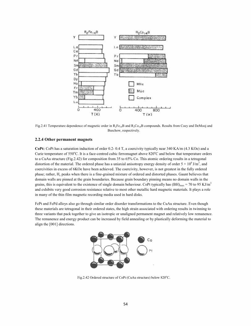
54

Fig.2.41 Temperature dependence of magnetic order in R2Fe14B and R2Co14B compounds. Results from Coey and DeMooj and Buschow, respectively.

2.2.4 Other permanent magnets

CoPt: CoPt has a saturation induction of order 0.2- 0.4 T, a coercivity typically near 340 KA/m (4.3 KOe) and a Curie temperature of 550oC. It is a face-centred cubic ferromagnet above 820oC and below that temperature orders to a CuAu structure (Fig.2.42) for composition from 35 to 65% Co. This atomic ordering results in a tetragonal distortion of the material. The ordered phase has a uniaxial anisotropy energy density of order 5 × 106 J/m3, and coercivities in excess of 6KOe have been achieved. The coercivity, however, is not greatest in the fully ordered phase; rather, Hc peaks when there is a fine-grained mixture of ordered and distorted phases. Gaunt believes that domain walls are pinned at the grain boundaries. Because grain boundary pinning means no domain walls in the grains, this is equivalent to the existence of single domain behaviour. CoPt typically has (BH)max = 70 to 95 KJ/m3

and exhibits very good corrosion resistance relative to most other metallic hard magnetic materials. It plays a role in many of the thin film magnetic recording media used in hard disks.

FePt and FePd alloys also go through similar order disorder transformations to the CuAu structure. Even though these materials are tetragonal in their ordered states, the high strain associated with ordering results in twinning to three variants that pack together to give an isotropic or unaligned permanent magnet and relatively low remanence. The remanence and energy product can be increased by field annealing or by plastically deforming the material to align the [001] directions.

Fig.2.42 Ordered structure of CoPt (CuAu structure) below 820oC.

55

MnALC Magnets The ordered FCT, CuAu phase of MnAl(τ) is ferromagnetic and metastable, forming by a martensitic transformation from the high temperature FCC phase. It has a uniaxial magnetic anisotropy of order 106 J/m3 and thus is of interest as a permanent magnet.

The addition of carbon leads to greater stability of the τ phase and the ability to induce [001] directional order by extrusion up to 700oC. Coercivites of 2 to 3 KOe and energy products of order (BH)max = 64 KJ/m3 are achieved in this largely single phase magnet.

Spinel Oxides Spinel cobalt ferrite, CoO.Fe2O3 shows a trigonal distortion and hence strong magnetocrystalline anisotropy relative to the undistorted spinels. High coercivity (up to 320 KA/m) has been speculated to be associated with pinning of domain walls on stacking faults. Pinning on stacking faults (planar defects typically 1 nm in thickness) would require an extremely strong anisotropy in the defect to pin a domain wall that would be about 10 times thicker. While not used commercially, cobalt ferrite appears to play the role of a compass in certain magnetotactic bacteria.

56

CHAPTER 3

PERMAET MAGET STABILITY AD LOSSES

57

3.1. Introduction

A compelling reason to use permanent magnets in many devices and systems is the magnet’s ability to maintain a constant flux output over a very long period of time. Nearly all applications subject the magnet to influence that tend to alter the magnet flux. If one knows the magnitude and nature of these influences, it is possible to predict the flux change. It is also possible, by exposing the magnet to these influences in advance, to render the magnet insensitive to subsequent changes in service. For many years, permanent magnets have exhibited long term stability in meters and instruments of the order of one part in 103. More recently, investigations in conjunction with inertial guidance systems for space vehicles have shown that long term stability of one part in 105 or 106 can be achieved. To attempt to achieve this order of stability with regulated electromagnets would be prohibitively complex and costly if, indeed, possible at all.

Today’s stability achievement with modern permanent magnets is in sharp contrast to very early permanent magnets in which both structural and magnetic changes caused a significant loss of magnetization with time.

3.2. Classification of magnetization changes

Magnet stability is a sophisticated subject and experience has shown it advantageous to classify these changes according to their nature and cause.

3.2.1.Reversible changes

The reversible changes in the magnetic properties of permanent magnet materials as a function of temperature originate in the change in spontaneous magnetization. These changes tend to obey the same temperature law as does saturation magnetization. Reversible changes are functions of temperature or circuit loading and are in no way time dependent. They disappear completely without need for re-magnetization when the permanent magnet is returned to its initial temperature.

3.2.2. Irreversible changes

In this type of change, after the removal of the disturbing influence the magnetization does not return to its original value. Examples of such changes are:

1.Ambient temperature; 2.Statistical local temperature fluctuations leading to viscosity effects, also known as after-effects; 3.Magnetic field-induced changes such as a change in magnetic circuit or exposure to an external field.

In this kind of change, the magnetization may be fully restored by re-magnetization.

3.2.3.Structural changes

Changes resulting from a permanent change in the structural or metallurgical state are generally time temperature dependent. Examples of such changes are:

1.Growth of precipitate phase;

2. Oxidation;

3.Annealing effects;

4.Increase in proportion of an ordered phase;

5.Radiation damage.

Re-magnetization does not restore the original state of magnetization after this kind of change. In the literature this type of change is often referred to as aging since there is time dependence. The temperature at which

58

changes in properties first become noticeable corresponds to the beginning of structural changes and corresponds closely to the maximum service temperature.

3.3.Temperature effects

Temperature changes bring about changes in a magnet’s properties. These changes are often complex and difficult to control. The different property systems give very different responses to temperature change. Thermal hysteresis effects as a result of temperature cycling also have to be controlled. 3.3.1. Effects of temperature on magnetization and coercive force

The relationship between intrinsic magnetization and temperature is predictable, in some cases the shape of the Bi versus T curves may be calculated, provided that there are details of the crystalline and magnetic structure of the phases present. In most cases such information is not available and instead direct measurements of Bi

versus T are made. The change of Bi with T depends on the extensive properties of the system, that is, particle size, internal field and domain structure. These changes generally must be determined experimentally for specific properties and geometries. For each material several values of length /diameter ratios are given so that the influence of B/H on the internal field can be noted. The changes of coercive force with temperature is a very important characteristic which is not well understood. The change of Hci with temperature may be predicted in some materials if detailed knowledge of the anisotropy temperature relationship is known. However, for most materials several anisotropies contribute to Hci and the resulting complexity leads to the need for direct measurements of Hci versus T.

3.3.2. Complete demagnetization curves at various temperatures

The temperature coefficients of magnetization and coercive force in many instances do not give enough information about how a magnet will respond to temperature change. In many magnets the demagnetization curve is not well defined by Br and Hci . Changes in the curve shape and the intersection with load lines can only be seen from a complete set of demagnetization curves measured at several different temperatures over the temperature range of interest. Fig.3.1 shows families of demagnetization curves at various temperatures for three different permanent magnet materials. These curves show a wide range of response to temperature change. For type I magnets where Hci˂˂Br and a knee is exhibited in the second quadrant for all temperatures, the normal demagnetization curves are all that the designer needs. For type II magnets with Hci ≥ Br both intrinsic and normal curves are required. In Fig.3.1 note that the coefficients for Bis and Hci are negative for the materials shown except that for ferrite the coefficient of Hci is positive.

59

Fig.3.1. Demagnetization at different temperatures for three different magnets: (a) Alnico5; (b) NdFeB; (c) Ceramic5.

3.4.Magnetic field effects

The level of flux supplied by a permanent magnet can be irreversibly changed by exposing the magnet to a field. The effect of external field while acting on the magnet and the final effects after its removal can be predicted. Intrinsic and normal demagnetization curves are shown in Fig.3.2a. Upon exposure to an external field, ∆H, the operating point moves down the curve and the change in intrinsic properties can be projected to the normal curve which shows a change ∆B occurring while the field is applied. The recovery along an interior loop when the field is removed is shown in Figure3.2b. ∆B is, of course, smaller than in Figure3.2a. Subsequent exposure to fields of lesser strength give small changes within the previously established minor loop, and upon removal, no change in

60

magnetization results. A given reverse field ∆H will cause different changes in ∆B depending on the permanence line. The loss will be greater when a magnet is operating in the steepest part of the demagnetization curve. Instead of exposing the permanent magnet to a field ∆H, the same effective stabilization will result if the air gap is increased and decreased so that the same minor hysteresis loop is established. For example, in the removal of a magnet from a magnetizing yoke and its subsequent transfer into an instrument gap and return path, stabilization is achieved.

Fig.3.2. Magnetic field effects. (a) Effects of a demagnetization field; (b) recoil of magnetization.

61

3.5.Temperature compensation

3.5.1. Compensation by compositional change

Compensation can be made at the atomic level . With SmCo5 and other light rare-earth compounds, the magnetic moment has a strong temperature dependence in the useful temperature range. There are rare-earth compounds containing Gd, Tb, Dy, Ho and Ey which exhibit a different temperature dependence because of a different mode of coupling between magnetic atoms. In Fig.3.3. the variation of magnetization with temperature is shown for SmCo5 , EyCo5 and GdCo5 . For the temperature range of interest (-40oC to +150oC) we should see that the light rare-earth compound has a negative temperature slope while the heavy rare-earth compounds have a positive slope. By combining both light and heavy rare-earth compounds, one can produce a near zero reversible temperature coefficient over a limited temperature range. However, the overall moment and resulting properties tend to be disappointing. For example, Sm0.7 Gd0.3Co5 results in only a 10 MGOe magnet. Our particular interest is to investigate temperature compensation in the Sm2(CoFe)17 alloy system. Leupold has reported that an alloy of composition Sm0.6Er0.4(CoFeCuZr)7.22 gave these magnetic properties Br= 9.3 KG, Hci =9.4 KOe, (BH)max =16.5MGOe, α=0.004% /oC. There appears to be most interest in compensation in the highest property materials although a substantial drop in properties is inherently the price paid for atomic alloy temperature compensation.

Fig.3.3 Comparison of magnetization changes for light and heavy rare-earth compositions.

3.6.Mechanical energy input and stability Mechanical shock and vibration add energy to a permanent magnet to decrease the magnetization in much the same manner as discussed for the case of the thermal after effect. Once difference is that the energy imparted thermally to the magnets is precisely KT, while the energy imparted mechanically is difficult to know with precision. Repetitive shock or vibration should reduce magnetization with the same logarithmic relationship as was the case for temperature. The time variable would be replaced with the number of impacts. Fig.3.4 shows some results for Alnico5 and earlier type magnets. There has been little study regarding stabilization due to the mechanical energy because with today’s high energy density magnets there is little need for concern. There is limited information which suggests that both thermal and field exposure will minimize but not entirely eliminate changes in magnetization due to shock.

62

Some magnet materials change properties when subjected to tension or compression. Vicalloy is one such material as shown in Fig.3.5.While man’s earliest magnets were magnetized and demagnetized by shocks in the earth’s field, today’s high coercive force magnets require very different energy input levels to change magnetization.

Fig.3.4 Flux Loss in bars dropped 1 m onto hardwood floors working at their (BH)m.

Fig.3.5 Effect of stress on Vicalloy. Applied stress of (a) 0; (b) 51; (c) 101; (d) 152; (e) 203; (f) 254 and 305 Kg/mm2.

3.7.Corrosion and surface oxidation

Alnico magnets are very resistant to corrosion, nearly as resistant as stainless steel. Only a slight discoloration of the surface is encountered when a magnet is heated in air to 450oC. Ferrite magnet surfaces are stable and not subject to oxidation. Rare-earth magnets have oxidation problems and this limits their maximum operating temperatures. Surface oxidation will lead to a reduction in magnetic output. Adler and Marik have studied this problem in depth and concluded that there are really three processes to distinguish: (i) selective surface oxidation; (ii) easy nucleation due to the deterioration of a surface layer with a thickness of a grain diameter and (iii) interior structural oxidation. In actual use, for SmCo5 up to 200oC , one has to be concerned mostly surface problems since interior oxidation will occur only at higher temperatures. As time and temperatures increase, oxygen diffuses into the material causing an oxidized layer to form. The thickness ds0 grows according to the relationship

This outer layer has a changed composition and a much lower coercive force so that the internal field of the magnet can reverse the magnetization of the outer layer. This leads to compounding of the flux loss of the magnet

63

since the outer layer represents a loss of flux because of the volume which is not effective and it also acts as a shunt in reducing the output of the interior magnet. SmCo5 magnets need some kind of protection above 200oC if structural change is to be avoided. The amount of protection needed will depend on the magnet’s surface to volume ratio. One effective form of protection is a heavy nickel plate. Kawashima has shown this form of protection effective for a travelling wave tube up to 300oC, as shown in Fig.3.6. Oxidation and corrosion are major problems is non-sintered rare-earth magnets. In a magnet with porosity, we have interior oxidation at much lower temperatures . To protect the fine particles is difficult and the form of protection occupies volume and hence severe property reduction is experienced.

Fig.3.6 exposure time dependence of peak axial field at 300oC. Changes are compared for a nickel-plated surface and an

untreated surface.

3.8.uclear radiation

There are a growing number of applications of magnets in nuclear environments. There are reported tests on both hard and soft magnetic materials. For soft magnetic material, the tests are quite conclusive in showing increased coercivity. For permanent magnets there is little evidence that the loss in flux output is anything beyond what can be attributed to temperature effects (Fig.3.7). The work reported to date does not clearly separate irreversibly loss from structural loss. Preliminary tests on NdFeB indicate they are inferior to the rare-earth cobalt magnets in terms of flux stability.

3.9.Enhancement stability

Permanent magnets have established a remarkable record with respect to maintaining constant flux over very long periods. There is still much further to go in terms of optimizing processing to focus on stability rather than property level. It appears that in the rare-earth cobalt magnets at least, and probably also with NdFeB , the most important properties to control are Hci and Hk to minimize short term irreversible losses. The order is important and square intrinsic demagnetization curves are desired. Another index is ∆s = HA (T)- Hk (T) The larger one can make ∆s by control of process and by magnetic circuit design, the less will be the irreversible loss. SmCo5 has been studied and concluded that instability in this material results from the formation of Sm2Co17 and Sm2Co7 phases. If the magnet is composed of stoic metric SmCo5 with low oxygen content that remains in solution at the operating temperature, then SmCo5 can offer much improved stability, coercivity, composition and structure. All appear to impart stability and high stability may only be achievable with some specific processing detail.

3.10. Stabilization techniques

When a magnet is newly magnetized and its flux level is observed over a long time period, one sees the relationship with respect to time as shown in Fig.3.8. There is initially an increase loss in a short time. This loss is irreversible and is followed by a relatively long period of near constant flux called the plateau. In this region the

64

loss per logarithmic cycle is constant. After long periods of time all materials at some higher temperature will exhibit a rapid flux decline. This is the region of structural change, perhaps oxidation or phase transformation. There is a temperature at which any magnet will undergo this kind of change. It may be polymer bonded SmCo5 at 75oC or Alnico 5 at 650oC. The example in Fig.3.9. is for SmCo5 at 250oC. The initial loss can be anticipated and stabilized against by heating to a temperature just above the expected operating temperature. One can pre-stabilize by applying an a.c. or d.c. field. Most, but not all of the reversible loss due to temperature will be eliminated. This field might also be combined with a temperature level above room temperature. In stabilizing against the after effect, an a.c field is most desirable. The alternating field is gradually reduced to zero or the magnet is slowly drawn from a field of constant magnitude in order to leave the magnet in a symmetrical state. As an alternative, the after-effect can be anticipated by holding at a temperature higher than Ta for a short time period .

Fig.3.7. Demagnetization of REC magnets due to proton irradiation.

Fig.3.8. Magnetic changes with time.

65

Magnetic stabilization tests for a cylinder SmCo5 having B/H =1.6 are shown in Fig.3.9. The stability conditions are described in the left position of the figure. One surprising result is increase in flux resulting when heating to 100oC and 200oC after a high level of field demagnetization. This thermal magnetization apparently results from a wide range of coercive force over the magnet volume. A near perfect crystal could have an anisotropy field of perhaps 100KOe surrounded by imperfect crystals having a much lower anisotropy field. When the temperature is raised the less perfect crystals are re-magnetized by the near perfect crystal region resulting in an overall increase of magnetization in the specimen. Or they can be used in combination. With high energy density magnets like rare-earth cobalt or NdFeB, it is sometimes advantageous to combine the energy sources so that, modest levels of each may be used in both magnetizing, demagnetizing and stabilizing.

Fig.3.9. Magnetic stability of SmCo5.

66

CHAPTER 4

APPLICATIOS OF PERMAET MAGET

67

4.1.Strong permanent magnet dipole with reduced demagnetizing effect

4.1.1 Introduction

Permanent magnet dipoles have many advantages over electromagnets. Permanent magnet dipoles do not require power supplies or cooling systems and are much more portable. The magnetic fields from permanent magnet dipoles are modest compared to the high field electromagnets. It can be a challenge to generate ever higher magnetic field with permanent magnets. In many applications such as magnetic wiggler for a storage ring or magnetic refrigeration where a strong field is required only in a small region, a permanent magnet dipole can still be used. The objective is to generate a magnetic field as strong as possible while maintaining the efficiency of the design. The residual induction of the strongest NdFeB magnet is about 1.4 T. To produce a magnetic field beyond its residual magnetization, one uses vector superposition in a permanent magnet dipole design. The most common and efficient design is the Halbach cylinder. The magnetization of each segment forming the Halbach cylinder is based on Halbach’s theorem to generate uniform field inside the cavity. The field magnitude can be much higher than the residual induction of the material.

Besides the Halbach array, other structures have been used to achieve strong fields with permanent magnets . A direct attempt using this structure is an extended Halbach cylinder. It uses a Halbach cylinder with iron poles as flux concentrators to increase the efficiency of the design. It achieved 3.9 Tesla. When the field uniformity is not critical, a common variation is the Stelter array. By using simple rectangular block magnets, the Stelter array is much easier to make than the Halbach cylinder. While its potential to achieve high field is equivalent to the Halbach cylinder, it sacrifices the field uniformity and efficiency. Another attempt used a variation of Halbach sphere to achieve 4.3 Tesla field within an air gap of 2.8 mm. It used a combination of NdFeB and SmCo magnets with FeCo pole piece. Two sub assemblies separated by an air gap of 2 mm were used in another design. The orientation of the magnets in each sub assembly all pointed to the centre where a FeCo rod was used as flux concentrator. This structure achieved a reported 5.16 Tesla with 2 mm air gap. A Halbach structure and its extended versions can be viewed as a multi-layer structure. Each layer is transparent to the magnetic field. The magnetic field from the outer layer is superimposed to the inner layer and so on. So in theory, the Halbach structures can generate infinitely strong magnetic field. But in reality, the magnets of the inner layers experience demagnetizing field from outer layers. So the field inside the cavity is limited by the ability of the inner magnets to resist demagnetization. This ability is tied to the intrinsic coercivity of the material. Assuming a 3 Tesla Halbach dipole with 3 layers, each generates 1 Tesla, then the reverse segments of the inner most layer will be subjected to 2 Tesla of demagnetizing field. So the intrinsic coercivity of the material for those segments needs to be over 2 Tesla in order to avoid reduced magnetization or even magnetization reversal. This effect will limit the ability to generate strong fields with permanent magnets. It is reported that, if the demagnetizing field is orthogonal to the orientation of the magnet, its ability to resist demagnetization can be nearly doubled . This property can be used for the inner layer of a dipole to greatly increase its ability to achieve higher field.

4.1.2. The principle of the design

The Stelter array is a variation of the Halbach structure that uses only 8 segments. In a Stelter array, tapered pole pieces are used to increase the field as well as the efficiency of the design. The segments that are opposite to the field in the cavity are subsequently tapered. A basic 2-D square Stelter array with square cavity is shown in Fig.4.1. In order to analyze the structure, we used current sheet equivalent are used for each segment. The current sheet equivalent of one pole magnet is also shown in Fig.4.1. Although the field in the cavity is not highly uniform as stated earlier, it is useful to calculate the field at the centre of the cavity so that we can evaluate its efficiency. Using current sheet equivalent, we can calculate the magnetic field at the centre of the cavity by each segment. Equation (1) shows the magnetic field by the basic Stelter dipole in Fig.4.1.

68

Fig.4.1. A square 2-D basic Stelter array with square cavity and current sheet equivalent of pole magnet.

K1 is a multiplying factor for Br to get the field inside the cavity. Although the field inside the cavity is not very uniform, it is still useful to use the figure of merit to evaluate the efficiency of the design. For the basic Stelter dipole shown in Fig.4.1, the figure of merit is

Ac is the cross sectional area of the cavity and Am is the cross sectional area of the permanent magnets. In the basic Stelter dipole, the inner sections of the two orthogonal or anti parallel segments will be under demagnetizing field from outer layers. Just as in a Halbach cylinder, these two segments are the main obstacle to achieve a strong field.

4.1.3.Selter dipole with orthogonal segments

In a modified Selter dipole, the 2 anti-parallel segments are replaced with segments that were oriented orthogonal to the magnetic field from outer layers. Fig.4.2 shows the proposed structure. On the left, the anti parallel segments were replaced with two orthogonal segments.

This change is equivalent to make the corner segments larger to fill the spaces of the anti-parallel segments as shown on the right side. With this change, the inclination angle of the magnetic field from outer layers is 90o with respect to the magnetic orientation of the corner magnets. Based on, the material can resist demagnetizing field of up to 170% of the intrinsic coercivity at this inclination angle. So this change makes it possible to achieve much higher field with permanent magnets. By using the current sheet method, we can calculate the magnetic field at the centre of the cavity for the 2-D square structure shown in Fig.4.2.

69

Fig.4.2. A square 2-D structure with orthogonal segments.

And the figure of merit of this structure is

4.1.4.Two-layer dipole by combining the two structures

To take advantage of the high resistance to demagnetizing field of the orthogonal segments, we propose a two layer structure is proposed combining the above two structures as shown in Fig.4.3. It is easy to see that, the magnetic field inside the cavity is the sum of the two. So the total field inside the cavity is

The figure of merit of the combined dipole structure is:

Fig.4.3. Two-Layer 2-D square dipole structure.

70

4.1.5.Construction of a prototype dipole with double layer structure

1. Optimization of the Pole Piece

We constructed a small prototype dipole with 3 Tesla desired field was constructed. For the prototype, low carbon steel pole pieces were used to increase its efficiency. The saturation of magnetization of a soft iron or steel piece is much higher than permanent magnets. Using a pole piece can increase the field in the cavity while reducing the amount of permanent magnet materials. The pole piece has a tapered shape as shown in Fig.4.4. Assuming the tapered pole pieces are uniformly saturated to its saturation magnetization Bs , using current sheet method for the 2-D structure in Fig.4.4, we find the magnetic field at the centre of the gap

By taking the derivative of (8) with respect to Ѳ, where is Ѳ the tapering angle (Fig4.4), we find the angle for Ѳmax maximum field

While this is true for two fully magnetized tapered pole pieces, the impact of this angle is diminished when the tapered pole pieces are incorporated into the double-layer structure shown in Fig.4.4.

Fig.4.4. Soft Iron tapered pole pieces.

2. The use of steel enclosure

In a perfectly aligned Halbach structure, the magnetic field outside the cylinder is zero. So a soft iron enclosure doesn’t affect the field inside the cavity. But in the 2 layer Stelter structures, there are leakage fields on outer surfaces of the corner and quad magnets. These leakage fields outside the dipole reduce the field inside the cavity. A steel enclosure shields the outside field, increasing the internal field, thus a steel enclosure is used. Moreover the orientation of the corner magnets is made 45 to the magnetic field inside the cavity.

71

4.1.6.Comparison and results

A. The prototype dipole

Fig.4.5 shows the structure of the prototype dipole. Fig.4.6 shows the actual prototype. This dipole uses tapered pole pieces as well as steel enclosures. The dimensions for the magnet package are 80 mm wide, 94 mm high and 76 mm long. The cavity is 5 mm × 5 mm × 76 mm long. The thickness of top steel plate is 12.7 mm and the thickness of the side steel plate is 19.05 mm. The magnet material is NdFeB with Br of 1.38 Tesla and Hci of 1276 kA/m. We calculated the field at the centre of the dipole results 3.167 Tesla, using commercial BEA software. Fig.4.7. shows the measured and modelled data along the centreline of the air gap. The measured data closely matches the modelled data. At the centre of dipole the measured field is 3.116 Tesla versus 3.167 Tesla modelled. While this is a good match to the modelled data, the difference was thought to be caused by the tolerance build up behind the pole pieces.

Fig.4.5 Structure of the prototype dipole Fig.4.6 Picture of the prototype dipole, the aluminium cover is on the side

Fig.4.7 Measured and modelled magnetic field of the prototype dipole.

B. Figure of merit comparison

For the prototype, the actual field is 2.258 times of the residual induction of the NdFeB magnet. The figure of merit of this prototype considering only permanent magnets is 0.019. The figure of merit of a perfect Halbach cylinder is

Fig.4.8. shows the figure of merit of the above structures comparing to the perfect Halbach cylinder. As expected, the efficiency of these structures is lower than a perfectly aligned Halbach cylinder. The dipole structure with orthogonal quad segments and the double layer structure are less efficient than the Stelter array. But with carbon steel pole pieces, the prototype dipole matches the efficiency of the Stelter array.

72

Fig.4.8. Figure of merit of the structures discussed.

73

4.2.Concentrated winding, axial flux, permanent magnet motor, with plastic bonded

magnets and sintered segmented magnets

4.2.1. Introduction

Sintered NdFeB magnets have a relatively high conductivity, that is, their resistivity is about 1.5 µΩm at room temperature. For comparison traditional construction steel Fe 52 (S355J0 / EN 10025) has a resistivity of about 0.25 µΩm which corresponds one sixth of the resistivity of NdFeB. Furthermore, the thermal conductivity of NdFeB is relatively poor, only about 9 W/mK which may cause problems with surface-magnet structures, since eddy currents caused by the spatial and current harmonics occur in the permanent magnet material. Because the heat conductivity is fairly poor and the power loss density may reach high values in the permanent magnet material, a fatal temperature rise in sintered bulky permanent magnets is possible. Fig.4.9 a) illustrates the rotor pole equipped with only one piece of surface mounted sintered NdFeB magnet and b) the rotor pole segmented 20 pieces of NdFeB magnet. Increase in temperature caused by eddy current losses can demagnetize the magnets and in any case reduce the efficiency of the machine. Plastic bonded magnets should offer a practically lossless alternative for the magnets, but the magnetic properties of the plastic bonded magnets available at the moment are still quite poor. For example, the maximum remanent flux density is usually well below 1 T, especially for the plastic bonded magnets tolerating temperatures above 100 °C.

Fig.4.9. a) Magnet is made of only 1 piece. b) magnet is segmented in 20 pieces.

4.2.2. Different analytical models for eddy current losses in permanent magnets

A concentrated wound stator produces a large amount of current linkage harmonics travelling across the permanent magnets causing eddy currents. Also, the large slot openings cause flux density variations that generate eddy currents in the permanent magnets. In inverter operation further eddy current losses are created by the time harmonics of the phase currents. However, they are analyzed in . Atallah, Ede and Toda presented an analytical method that could be utilized to calculate eddy current losses in radial flux permanent magnets caused by stator magneto-motive force space harmonics. However, the effect of the stator slot openings was not considered. The results from the analytical calculations were compared with finite element analysis (FEA) calculations with unmagnetized permanent magnets. Polinder and Hoieijmakers assumed that the magnet losses in radial flux permanent magnet machine caused by the space harmonics of the stator windings and the stator slotting are negligible. The approximation in this equation is based on the assumption that the magnet width is small. The results were compared with FEA calculations with unmagnetized permanent magnets. The analytical calculation method for eddy current losses in permanent magnets with axial flux machine is presented by Gieras.

4.2.3.Finite element methods

Eddy current losses in permanent magnets of 2500/3000 rpm and 37 kW permanent magnet synchronous motors with concentrated windings were calculated by using two dimensional (2D) finite element analysis.

74

Magneto-static and magneto-dynamic time stepping method is used. The Joule losses in the magnets caused by the eddy currents are calculated in the FEA

where ρm is the material resistivity, V the volume and J the current density.

4.2.4. Results of FEA and analytical calculations

Fig.4.10. shows a comparison of the air gap flux density waveforms and Fig.4.11. shows a comparison of the phase back electromotive force waveforms, for the rotor pole equipped with only one piece of surface mounted sintered NdFeB magnet and the rotor pole which is segmented into 20 pieces of NdFeB magnet. NdFeB magnet remanent flux density used is Br = 0.9 T @ 120ºC (Br = 1.05 T @ 20ºC). The FEA calculation was done by using a 2D solution. Fig.4.10and Fig.4.11 show the effect of the segmented magnets. It can be seen in Fig.4.10, that there is a small ripple in the air gap flux density which is caused by air between segmented magnets. It is shown in Fig.4.10, that the amplitude of the back emf is a bit smaller with segmented magnets than the one magnet per pole version.

Fig.4.10. Comparison of the air gap flux density distribution for only one piece of surface mounted sintered NdFeB magnet and for the pole segmented in 20 pieces of NdFeB. Rotational speed is 2500 rpm and magnetic flux density 0.9 T.

Fig.4.11. Comparison of the induced phase-EMF voltage waveforms for only one piece of surface mounted sintered NdFeB magnet and for the pole segmented in 20 pieces of NdFeB. Rotational speed is 2500 rpm and magnetic flux density 0.9 T.

Fig.4.12. shows the eddy current losses in permanent magnets calculated using 2D-FEA. FEA calculation was done for three different methods. FEA results utilizing no load method take into account only eddy current

75

losses caused by the stator slot openings. Magneto-dynamic calculation using unmagnetized magnets takes into account only the eddy current losses caused by stator magneto-motive force space harmonics. Load method takes into account both the aforementioned loss components. In Fig.4.13. it is shown that the slot openings have significant effect on eddy current losses in permanent magnet. Those losses are bigger than the eddy current losses that were caused by stator magneto-motive force space harmonics. Those losses could be reduced using semi closed slot, but then the machine winding manufacturing process is not so easy. Fig.4.14. shows the comparison of the different analytical methods and FEA 2D when magnets are unmagnetized. This situation takes into account only the eddy current losses caused by stator magneto-motive force space harmonics.

Fig.4.12. Eddy current losses in magnet using FEA 2D method in three different conditions, no load, un magnetized and

load situations.

Fig.4.13. Eddy current losses in un magnetized for three different methods: Atallah, Polinder and 2D FEA.

Fig.4.13. shows the comparison of analytical method and FEA 2D. This situation takes into account the eddy current losses caused both by stator magneto-motive force space harmonics and by stator slot opening. In Figs.4.13.and 4.14 it can be seen that the analytical methods shown are in good agreement with FEA results especially with segmented magnets. The first two analytical methods can be used as an estimation of the eddy current losses in the segmented magnets when unmagnetized, that is the eddy current losses caused by stator magneto-motive force space harmonics . The third analytical method can be used as an estimation of the total eddy

76

current losses in permanent magnets. The influence of skin effect and saturation are neglected in the analytical models.

Fig.4.14. Eddy current losses in magnets in load situation for two different method: FEA2D and Gieras.

4.2.5. Results of prototype Fig.4.15. and 4.16. show two different views of the 37 kW plastic bonded magnet prototype machine. The machine is a double stator axial flux machine with 12 slots and 10 poles. Magnets are assembled on the rotor surface and open stator slots structure is used. The motor is air cooled by a fan.

Fig.4.15. The stator of the prototype machine. Fig. 4.16.Prototype machine assembled. Figs.4.17 and 4.18. shows the measured phase back-emf voltages with plastic bonded magnets compared to the FEA results. The FEA calculation is done by using 2D (Fig.4.17.) and 3D solutions (Fig.4.18.)

77

Fig 4.17 Comparison of calculated (FEA 2D) and measured phase back-emf voltages at 3000 rpm with plastic bonded magnets.

Fig. 4.18. Comparison of calculated (FEA 3D) and measured induced phase back-emf voltage waveforms at 3000 rpm with plastic bonded magnets. Figs.4.17. and 4.18. it can be seen that the measured and FEA (2D and 3D) calculated back-emf waveforms are quite similar. Some of the measurement results of the prototype machine are listed in table 4.1. The half power was used in the first measurement. The results have good agreement with analytical calculations with half power. Table 4.1 Measurement results with plastic bonded machine with half power

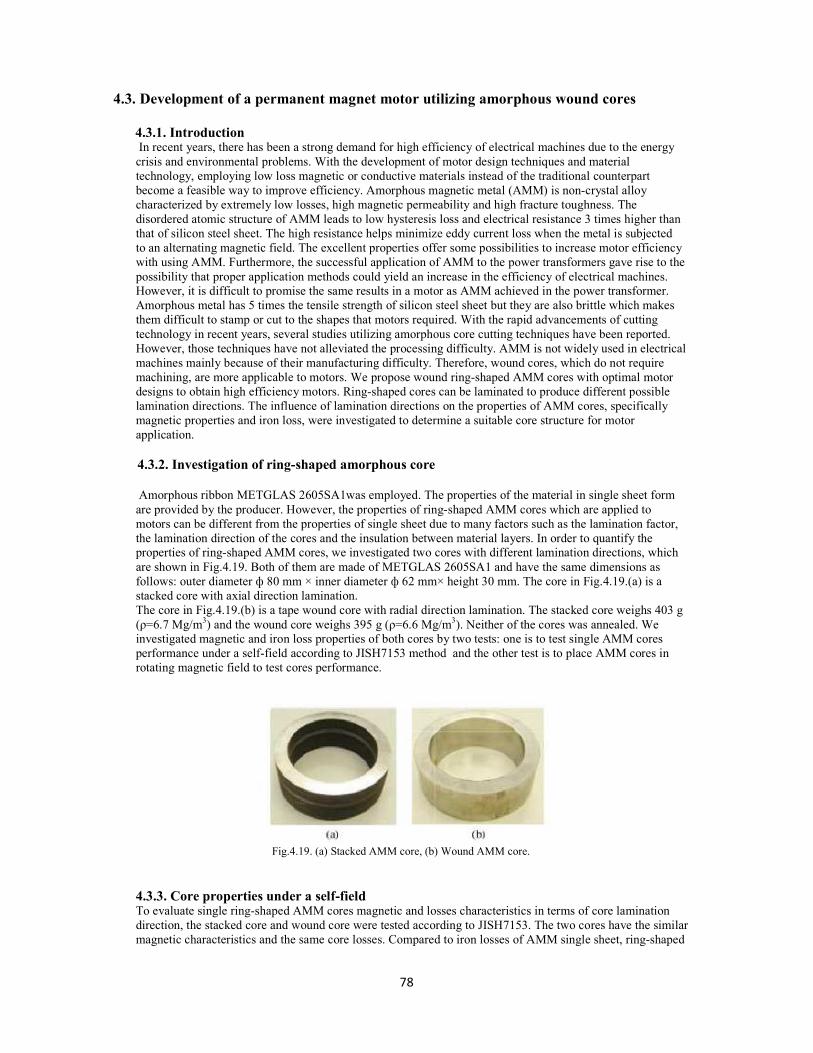
78

4.3. Development of a permanent magnet motor utilizing amorphous wound cores

4.3.1. Introduction

In recent years, there has been a strong demand for high efficiency of electrical machines due to the energy crisis and environmental problems. With the development of motor design techniques and material technology, employing low loss magnetic or conductive materials instead of the traditional counterpart become a feasible way to improve efficiency. Amorphous magnetic metal (AMM) is non-crystal alloy characterized by extremely low losses, high magnetic permeability and high fracture toughness. The disordered atomic structure of AMM leads to low hysteresis loss and electrical resistance 3 times higher than that of silicon steel sheet. The high resistance helps minimize eddy current loss when the metal is subjected to an alternating magnetic field. The excellent properties offer some possibilities to increase motor efficiency with using AMM. Furthermore, the successful application of AMM to the power transformers gave rise to the possibility that proper application methods could yield an increase in the efficiency of electrical machines. However, it is difficult to promise the same results in a motor as AMM achieved in the power transformer. Amorphous metal has 5 times the tensile strength of silicon steel sheet but they are also brittle which makes them difficult to stamp or cut to the shapes that motors required. With the rapid advancements of cutting technology in recent years, several studies utilizing amorphous core cutting techniques have been reported. However, those techniques have not alleviated the processing difficulty. AMM is not widely used in electrical machines mainly because of their manufacturing difficulty. Therefore, wound cores, which do not require machining, are more applicable to motors. We propose wound ring-shaped AMM cores with optimal motor designs to obtain high efficiency motors. Ring-shaped cores can be laminated to produce different possible lamination directions. The influence of lamination directions on the properties of AMM cores, specifically magnetic properties and iron loss, were investigated to determine a suitable core structure for motor application.

4.3.2. Investigation of ring-shaped amorphous core

Amorphous ribbon METGLAS 2605SA1was employed. The properties of the material in single sheet form are provided by the producer. However, the properties of ring-shaped AMM cores which are applied to motors can be different from the properties of single sheet due to many factors such as the lamination factor, the lamination direction of the cores and the insulation between material layers. In order to quantify the properties of ring-shaped AMM cores, we investigated two cores with different lamination directions, which are shown in Fig.4.19. Both of them are made of METGLAS 2605SA1 and have the same dimensions as follows: outer diameter ф 80 mm × inner diameter ф 62 mm× height 30 mm. The core in Fig.4.19.(a) is a stacked core with axial direction lamination. The core in Fig.4.19.(b) is a tape wound core with radial direction lamination. The stacked core weighs 403 g (ρ=6.7 Mg/m3) and the wound core weighs 395 g (ρ=6.6 Mg/m3). Neither of the cores was annealed. We investigated magnetic and iron loss properties of both cores by two tests: one is to test single AMM cores performance under a self-field according to JISH7153 method and the other test is to place AMM cores in rotating magnetic field to test cores performance.

Fig.4.19. (a) Stacked AMM core, (b) Wound AMM core.

4.3.3. Core properties under a self-field To evaluate single ring-shaped AMM cores magnetic and losses characteristics in terms of core lamination direction, the stacked core and wound core were tested according to JISH7153. The two cores have the similar magnetic characteristics and the same core losses. Compared to iron losses of AMM single sheet, ring-shaped

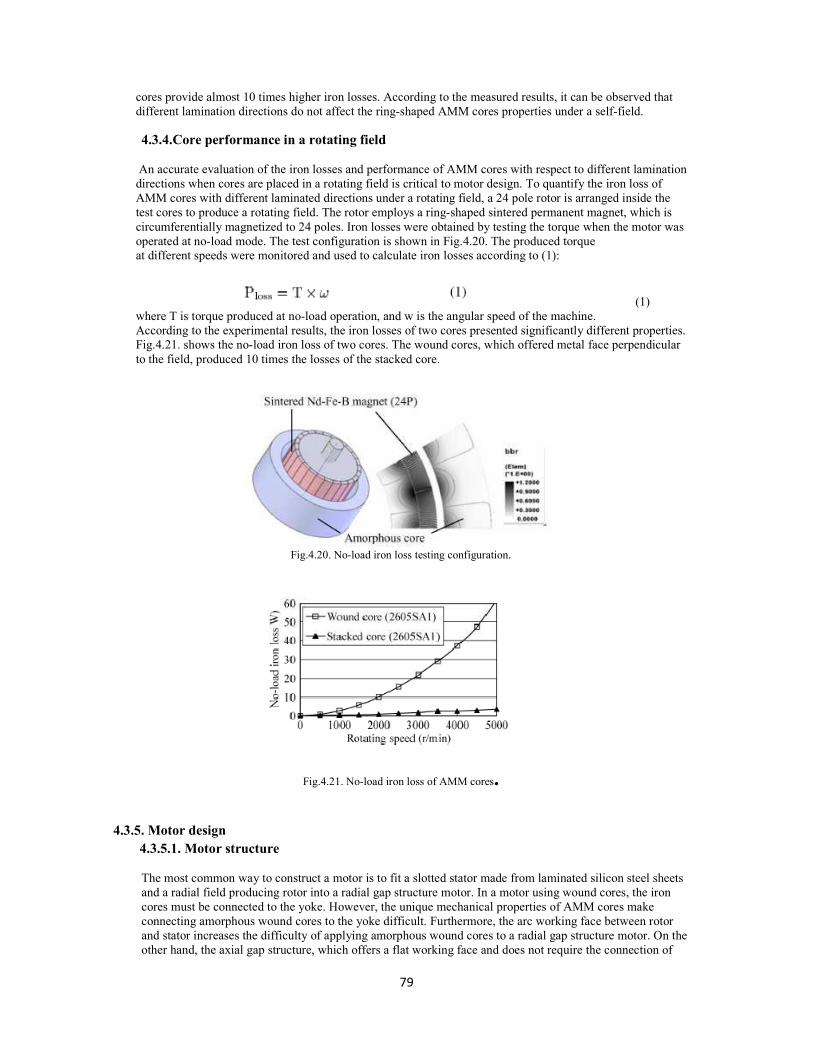
79

cores provide almost 10 times higher iron losses. According to the measured results, it can be observed that different lamination directions do not affect the ring-shaped AMM cores properties under a self-field.

4.3.4.Core performance in a rotating field

An accurate evaluation of the iron losses and performance of AMM cores with respect to different lamination directions when cores are placed in a rotating field is critical to motor design. To quantify the iron loss of AMM cores with different laminated directions under a rotating field, a 24 pole rotor is arranged inside the test cores to produce a rotating field. The rotor employs a ring-shaped sintered permanent magnet, which is circumferentially magnetized to 24 poles. Iron losses were obtained by testing the torque when the motor was operated at no-load mode. The test configuration is shown in Fig.4.20. The produced torque at different speeds were monitored and used to calculate iron losses according to (1):

(1) where T is torque produced at no-load operation, and w is the angular speed of the machine. According to the experimental results, the iron losses of two cores presented significantly different properties. Fig.4.21. shows the no-load iron loss of two cores. The wound cores, which offered metal face perpendicular to the field, produced 10 times the losses of the stacked core.

Fig.4.20. No-load iron loss testing configuration.

Fig.4.21. No-load iron loss of AMM cores.

4.3.5. Motor design

4.3.5.1. Motor structure

The most common way to construct a motor is to fit a slotted stator made from laminated silicon steel sheets and a radial field producing rotor into a radial gap structure motor. In a motor using wound cores, the iron cores must be connected to the yoke. However, the unique mechanical properties of AMM cores make connecting amorphous wound cores to the yoke difficult. Furthermore, the arc working face between rotor and stator increases the difficulty of applying amorphous wound cores to a radial gap structure motor. On the other hand, the axial gap structure, which offers a flat working face and does not require the connection of

80

wound cores and yokes, makes constructing a motor using amorphous wound cores less difficult. Reference , which covered research on the radial and axial field motors, show that axial-gap motors are compact, have high torque outputs, and a high power density. To create a simple structure motor and avoid connecting AMM wound cores with yokes, an axial gap synchronous motor with an amorphous cores stator and two permanent magnets rotors was designed. A design of 8 pole, 12 slot is proved to be the best balanced combination within 100 mm of motor target outer diameter. The 3-D model of the motor is shown in Fig.4.22. 1) Rotor: In this design, a pair of 8 pole rotors with sintered ferrite magnets were employed. 8 pole rotors guarantee changeless performance during reverse rotation. 2) Stator: The stator includes twelve amorphous tape wound AMM cores coupled with concentrated copper coils. To decrease eddy current loss, the lamination direction of AMM core was designed perpendicular to the field produced by rotors.

Fig.4.22. Three dimensional model of motor

4.3.5.2. Motor equations

The rough calculation of motor parameters can be derived from the motor design equations which are shown as follow. The electromotive force (EMF) induced in one stator coil by air gap flux ф produced by rotor field can be expressed as:

Where the w is the angular speed of the machine; p is the number of pole pairs; N is the number of turns of each stator coil; Poutput is the output of motor; n is the number of stator coils.

4.3.5.3. Trial motor

Fig.4.23. shows the rotor and stator of the trial motor. Eight parallel magnetized ferrite magnets are fixed on the iron rotor yoke. The stator core is wrapped from AMM tape and vacuum infused with resin for insulation between amorphous layers. The cores are wound without adhesive to increase the lamination factor. Fig.4.24. shows the wrapping process and the moulded core. Due to the incompletely insulation between amorphous layers, eddy currents produced on the lamination face, which is shown in Fig.4.24 (b). To reduce the eddy current loss, a section of core was removed to cut off the current loop. Fig.4.25. shows the pictures of a new core with a section removed. After twelve coiled amorphous cores are arranged and wire connected, the stator assembly is moulded by resin. The rotor is placed to produce an air-gap field tangential to the amorphous face to prevent eddy current produced.

81

Fig.4.23. (a) Rotor of the motor, 8b) Stator of the motor

Fig.4.24. (a) wrapping process, (b) Moulded AMM core.

Fig.4.25. (a) AMM wound stator core, (b) assembly of AMM core and copper coil.

4.3.5.4.Test result No-load tests and load tests were conducted to evaluate motor performance. With new AMM cores, iron loss of trial motor decreased drastically. The iron loss distributions of cores at different rotating speeds before and after a section was removed are shown in Fig.4.26. The measured EFM is 18.9 Vrms at 1000 r/min, which is 5% different from the calculated value, 19.7 Vrms. The comparison results are shown in Table 4.2. As can be seen, the calculated and measured results have a good correspondence, which proved the accuracy of the 3-D FEA. The measured motor efficiency is 86% at the most and 85% at rated conditions. Compared to the industry leading level of fan motors , which offers 200 W with 85% efficiency by utilizing neodymium (Nd) permanent magnets, this motor achieved a high efficiency with ferrite magnet.

Fig.4.26. No-load iron loss distribution of AMM cores.

82

Table 4.2. Comparison of motor parameters

83

4.4 Permanent magnet for micro electro-mechanical systems

4.4.1. Introduction

Permanent or “hard” micro-magnets are a critical enabling component for the development of high performance micro scale magnetic machines such as motors, generators, switches, pumps, acoustic speakers, and energy harvesters. An analysis of physical scaling laws reveals the importance of permanent magnets for micro scale applications . Magnetic fields from a current carrying electromagnet unfavourably scale with diminishing size, whereas the fields from a permanent magnet are scale invariant, at least down to a certain point. The source of magnetic fields in an electromagnet is the current, which, in a non-superconducting material, is a dissipative process and, thus, thermally limited. This sets a practical limit on the suitability of micro coils for generating magnetic fields via electrical currents. The methods for magnet fabrication at the macro scale, i.e., casting and powder processing, are starkly foreign to traditional thin film micro-fabrication approaches, i.e., physical vapour deposition, chemical vapour deposition, and electrochemical deposition. While there is a wealth of information on both soft and hard magnetic thin films as it relates to magnetic media, these films are too thin (often less than 100 nm) to be applicable for most magnetic micro-electromechanical systems (MEMS). For example, it has been argued that magnetic actuators are more favourable than electrostatic actuators when the actuation gap is greater than ∼2 µm. This implies the need for relatively voluminous (thick) magnetic structures to establish reasonably strong magnetic fields over multi-micrometer-length. The application and integration of hard magnets in MEMS present even more design and fabrication challenges. 1) Unlike soft magnetic films, there is no pre-existing knowledge base from which to draw. The need for relatively thick films of hard magnetic materials is somewhat unique to MEMS applications. 2) Like soft magnets, there are different classes of hard magnetic materials, each with strengths and weaknesses. The magnetic performance, temperature effects, chemical stability, and fabrication constraints all play a role in the material selection and micro-fabrication strategy. 3) The material properties of most hard magnets are typically quite sensitive to both the microstructure and the chemical composition. This requires careful control over the processing conditions and may require the application of magnetic fields, additional thermal steps, or other processing steps to induce optimal magnetic properties, thus adding cost and complexity to the fabrication. 4) Hard magnets require post fabrication magnetization steps to “pole” the magnets in a specific direction. This complicates the integration process, particularly for wafer-scale batch fabrication. It also usually implies that all magnets on a wafer are magnetized in only one direction, which restricts the device design. 5) Perhaps most importantly, the total system performance of a permanent-magnet-based system is usually limited by the magnet. Thus, the quality and performance of the magnetic material play a critical role in the overall design.

4.4.2. Requirements The application of permanent magnets at the micro scale requires many considerations. Most MEMS devices and process flows are highly custom and application specific. Each system has different needs and different constraints (size, performance, temperature range, cost, process limitations, etc.). Thus, no single magnetic material or fabrication process will meet all needs. However, there are some general goals that are common to many MEMS platforms. Before delving into previously published results, it makes sense to first describe rough targets for the desired properties and to provide examples of trade off in the selection of suitable magnetic materials.

4.4.2.1.Magnet size

For MEMS device design, relatively large magnetic volumes are often desired to achieve large magnetic fields, magnetic forces, or electromechanical energy exchange. For example, unlike electrostatic forces, which are dependent on the surface area, magnetic forces depend on the volume. Additionally, one often-touted advantage of a magnet is the ability to create magnetic fields over fairly long distances, e.g., for actuators with large working gaps. However, the magnetic field emanating from the surface of a magnet rapidly decays with distance. While it is possible to achieve strong magnetic fields over relatively long distances, this requires magnets of substantial size. Typical magnet dimensions required for MEMS range from a few micrometers to hundreds of micrometers or possibly even larger, depending on the application.

84

4.4.2.2.Material performance

For functional use, a magnet should exhibit strong magnetic properties and suitable thermal and chemical stability for the intended application. General material trade off are well documented for bulk materials. For micro scale magnets, the temperature stability and the chemical stability are generally similar to the macro scale material properties. However, the magnetic performance of micro scale magnets is often lower than that in bulk, largely due to process and integration constraints (further discussed below). A decent-quality micro scale magnet could be expected to have Hci > 200 kA/m, Br > 0.5 T, and (BH)max >

30 kJ/m3, which is roughly the performance of a bulk ferrite magnet. One additional consideration relating to material performance is the ability to control the direction of magnetic anisotropy either during or after deposition. Certain magnetic films and deposition processes lead to better in plane performance, whereas others exhibit better out of plane performance. Isotropic materials are also possible, but these are usually of lower quality. These considerations affect material selection and the overall device design. The strength and direction of anisotropy can be influenced by the deposition temperature or post deposition annealing, the application of magnetic fields during deposition, substrate crystalline via lattice templating, or the material microstructure, e.g., needle like in-plane structure versus column like out-of-plane structure. Furthermore, while chemical reactivity is expected to be about the same between macro scale and micro scale magnets, corrosion/oxidation effects become more important at small size scales, where surface area to volume ratios become large. For example, a 50 µm-thick “skin” of oxidation may be tolerable on a 1 cm3

magnet, but it is certainly not tolerable in a 100 µm-thick magnetic film, since half of the film would no longer be magnetic.

4.4.3.Process integration One of the biggest challenges for realizing micro scale magnetic systems is process integration. Unlike bulk magnetic devices where magnets are separately manufactured and then assembled into the final system, micro-fabrication demands monolithic integration of the magnets within a multistep sequential process flow. This integrated manufacturing approach places constraints on the magnetic materials and processes that are not normally found in macro scale manufacturing. First, wafer-level deposition processes are desired to maintain the cost, throughput, and repeatability advantages afforded by batch fabrication. As previously described, most macro scale magnets are manufactured using processes (casting and powders) that are very different from those commonly employed in micro fabrication. Thus, to be suitable for micro system integration, different processing approaches are needed. Second, deposited micro magnets should be lithographically defined to form precise aligned geometries for device design. This requires methods for selective deposition (e.g., electroplating and screen printing) or selective etching of blanket deposited magnetic layers. Chemical etchants for many of the complex magnetic alloys are not widely known, so selective deposition may be preferred. Third, the magnets should be deposited at low temperatures and avoid post annealing requirements, so other integrated circuits or common MEMS materials (e.g., polymers and Al) can survive the process conditions. Ideally, room temperature processes are preferred, but at minimum, processing temperatures should be kept below 450oC for potential post complementary metal oxide semiconductor compatibility. Fourth, not only should the deposition of the magnets not affect pre-existing structures on a wafer, but the deposited magnets must also be stable enough to survive any subsequent processing steps (e.g., photolithography, chemical etching, plasma processes, and thermal steps). Last, micro-fabricated magnets require a magnetization step after fabrication. To maintain wafer level processing, this usually implies magnetization in only one direction. Although it is not impossible, it is difficult to magnetize magnets in different directions when they are in close proximity and share a common substrate. All of these integration issues place strict limitations on material selection and fabrication methods, not to mention constraints on device design. For example, metal alloys can be deposited by electro deposition or physical vapour deposition. Electroplating offers a relatively low cost high deposition-rate approach for achieving multi micrometer films, as well as the ability to selectively deposit material using photo resist masks. In contrast, vapour deposition is usually slower and more costly and requires post deposition etching or polishing steps to define the pattern since standard “lift-off” methods may not work with thick layers. While electroplating may seem to be highly desirable, it requires careful control over many process parameters and often suffers from lack of repeatability. Additionally, ferrites and rare-earth magnets cannot be electrodeposited from aqueous solutions, so vapour deposition or other methods are necessary. In general, there are many trade off in the selection of a material and fabrication approach.

85

4.4.4.Micro fabricated permanent magnets With a general understanding of magnetic materials and the hurdles for application at the micro-scale, this section now presents a review of permanent magnet materials suitable for MEMS integration. This summary is restricted to permanent magnets that can be deposited or grown on typical MEMS substrates (e.g., Si, glass) and have film thickness values of at least 0.5 µm. This specifically excludes magnets that require manual assembly for integration, magnets on “exotic” substrates, and very thin magnetic films.

4.4.4.1.Conventionally deposited micro-magnets Conventional deposition encompasses physical vapour deposition [sputtering, evaporation, and pulsed-laser deposition (PLD)] and electrochemical deposition (electroplating). These wafer level batch fabrication processes are familiar to the MEMS community and have enabled a large majority of the prior investigations into micro-magnets. Table 4.3 summarizes many conventionally deposited magnets. In many cases, remanence values and energy products were not reported. Of the various magnetic material categories, metal-alloy magnets have been the most widely studied for potential integration in MEMS, primarily because of the favourable cost, simplicity, and process integration afforded by electro-deposition. The earliest efforts for integrating permanent magnetic materials for MEMS focused on Co–Ni–X alloys, where X is normally a nonmagnetic element such as P and W. These nonmagnetic elements are usually very small in relative quantity but important. During electroplating, these elements tend to segregate at grain boundaries, forming defects that inhibit domain walls from moving, hence increasing the coercivity. However, the resulting magnetic properties are usually fairly limited. The intrinsic coercivities are usually in the range of 30–200 kA/m, and the energy products are usually less than 10 kJ/m3. Despite this modest performance, these films are readily integrated into MEMS processes using straightforward electro-deposition methods. Motivated by the successful application in the magnetic recording area, deposition of equi-atomic ordered L10 CoPt and FePt films have also been investigated. L10 refers tetragonal distortion of a face-centred cubic structure, where atomic layers of Pt are sandwiched between Fe (or Co) layers. Relatively thick films have been deposited by electroplating, sputtering and PLD, but high-temperature annealing (generally 400oC–800oC) is usually required to induce the ordered L10 structure. Intrinsic coercivities of up to 1440 kA/m and energy products of up to 124 kJ/m3 have been achieved after annealing. Recently, Nakano has reported FePt thick films having the L10 phase without intentional substrate heating, although it was unclear if the substrate became hot during deposition to induce the L10 ordering. High power PLD was used to deposit an area of 5 × 5 mm2, resulting in an out of plane energy product of up to105 kJ/m3. Another metal alloy is the Co-rich CoPt system, where the Co content is approximately 80%. This alloy offers strong magnetic properties as in the deposited state, i.e., without any high temperature annealing. Strong out-of-plane magnetic anisotropy is achieved by aligning the c-axis of the Co crystalline perpendicular to the substrate and encouraging a columnar microstructure with phosphorous segregated grain boundaries. This process is enhanced by using textured seed layers, e.g., Cu (111) on Si (110), that provide a template lattice for the desired crystalline structure. Wang and Arnold demonstrated 8 µm thick patterned films with an energy product of 69 kJ/m3. While great strides have been made with metal alloy magnets, their properties are still fairly limited. As a result, interest has steadily grown in rare-earth magnetic materials. Since rare-earth magnets cannot be electroplated from aqueous baths, most efforts have employed sputtering or PLD. In the materials community, the magnetic properties of rare-earth thin films (< 0.5 µm) have been shown to approach that of bulk magnets. Technical challenges such as control over stoic metric, the crystal structure, and the microstructure have been overcome, and protection layers (to mitigate oxidation and corrosion) are readily deposited on top of the magnetic films. Unfortunately, less attention has been paid to thicker films and MEMS integration issues (patterning, batch fabrication, and deposition rate). Recently, however, investigations have begun focusing on increasing deposition rates and developing wafer level deposition processes with specific intent for MEMS applications. SmCo alloys are first discussed. Prados demonstrated fairly thin (0.5 µm) sputtered SmCo films with a very high intrinsic coercivity of 2080 kA/m after annealing at 550oC. Fabricated thicker (1.5 µm) films were realized by sputtering SmCo onto a heated substrate followed by annealing at 550oC. They reported an impressive intrinsic coercivity of 2100 kA/m, but unfortunately, no remanence or energy product was provided. Budde and Gatzen sputtered SmCo films at deposition rates of 2.9 nm/s up to 50 µm in thickness on glass and alumina substrates. A maximum energy product of 90 kJ/m3 was achieved for 30-µm-thick films after post-deposition annealing at 560oC. Walther demonstrated 5-µm-thick films on silicon, which, after annealing at 750oC, exhibited a modest intrinsic coercivity of 1035 kA/m but has a high energy product of 140 kJ/m3. Last, in an attempt to

86

mitigate oxidation effects, Cadieu deposited nano phase SmCo into a metal matrix using PLD. The final composite film, which was deposited at 435oC and annealed at 550oC, had a thickness of 1 µm and an intrinsic coercivity of 1200 kA/m.

Compared to SmCo, NdFeB alloys are more susceptible to oxidation, so additional coatings and protection layers are crucial. Yamasawa reported a 1µm thick sputtered multilayer structure with alternating layers of W and NdFeB, where the W acted to limit the oxidation of the Nd. The layers were deposited at 450oC with resulting energy products of 50 kJ/m3. Castaldi explored Cu and Nb buffer and cap layers on 1µm thick NdFeB films sputtered at 470oC, resulting in an energy product of 150 kJ/m3. Dempsey developed a dc triode sputtering technique to produce 5µm thick NdFeB thick films at deposition rates up to 5 nm/s. The reported energy product after 750oC annealing was as high as 400 kJ/m3, which is comparable to bulk rare-earth magnets. Nakano demonstrated extremely thick PLD NdFeB layers of up to 120 µm. However, this method has been limited to fairly small deposition areas and modest energy products (77 kJ/m3). While the magnetic properties of SmCo and NdFeB thick films are very attractive, the etching and patterning of these films remains somewhat challenging. Budde and Gatzen reported methods for patterning thick SmCo films by ion beam etching (20 nm/min) or wet chemical etching using ammonium cernitrate (12.5 µm/min). The ion milling was prohibitively slow, and the wet etching suffered from high lateral etch rates, resulting in poor dimensional control. Walther has patterned SmCo and NdFeB by filling pre-etching trenches in the substrate, followed by chemical mechanical planarization in a Damascene-like process. After thermal annealing, film fracture occurred on the SmCo films but not on the NdFeB films. Wet etching using (NH4)2S2O8 · H2O and H2SO4 has also proved suitable for both NdFeB and SmCo films in the amorphous state (before annealing). Vertical sidewalls were achieved on 5 µm thick films, with etch rates of 1.25 µm/min. However, a large lateral overreach of 20 µm was observed in both materials. In summary, the simple CoNi alloys are readily integral but fundamentally limited in performance. The better performing FePt L10 alloys and rare-earth alloys require annealing at high temperatures (> 400oC) to achieve their high magnetic properties, so the thermal budget and process integral must be considered. The rare-earth materials have also proven to be difficult to pattern. The middle ground in performance is occupied by the Co-rich CoPt alloys, which exhibit good performance in the as deposited state and are integral via room temperature electro-deposition. Furthermore, with the exception of the CoNiMn alloys, which have relatively low magnetic performance, most of the better performing sputtered or electroplated films are limited to a few micrometers in thickness. This is due to intrinsic stresses that develop during deposition and/or thermal mismatch stresses that arise during annealing steps. Furthermore, the magnetic performance of a film tends to degrade with thickness due to variations in the microstructure, e.g., grain size and shape.

87

Table 4.3 Conventionally micro-fabricated permanent magnet for MEMS.

4.4.4.2Powder micro-magnets While the use of magnetic powders is ubiquitous for macro-scale magnet fabrication, their use in micro-fabrication is certainly a foreign concept. The idea of intentionally introducing small powder particles into a “clean” environment is sure to raise eyebrows with clean room managers. Despite the potential segregation/contamination issues, the magnetic properties of bulk manufactured powder based magnets are too attractive to overlook. If suitable integration methods can be developed, the complex high temperature material processing steps required to achieve ideal magnetic properties can be delegated to the powder manufacturing, separately from the MEMS fabrication. Additionally, the use of magnetic powders affords the opportunity to batch fabricate magnets with thickness values that are not technologically feasible with other standard micro-fabrication or bulk manufacturing methods. As previously described, sputtered or electroplated magnets are often limited to a few micrometers in thickness, while bulk manufacturing technique do not enable magnets much smaller than 1 mm. Thus, micro-scale powder processing methods may be well suited for magnets in the range of 10 µm–1 mm. Naturally, the magnetic particle size dictates the minimum magnetic feature size. The particles must be smaller than the desired feature size to ensure a quasi-homogenous distribution of particles. Commercially available hard ferrite powders are available down to ∼2 µm, Sm–Co powders are available down to 5–10 µm, and NdFeB powders are available down to ∼50 µm. The minimum particle size is dependent on the combination of the micro-structural grain size, the magnetic domain size, and thermal stability . As summarized in Table4.4, attempts have been made to incorporate magnetic micro-particles into micro-fabrication processes in several ways. In one approach, which was coined magnetic composite electroplating by Guan and Nelson, non soluble magnetic particles were incorporated into conventional magnetic alloy electroplating baths to create metal particle composites. During deposition, the magnetic particles (e.g., BaFe12O19) were mechanically and electrochemically captured into the growing electro deposit. So far, this approach has achieved energy densities of up to 6–9 kJ/m3 for arrays of magnets that are 15–50 µm thick

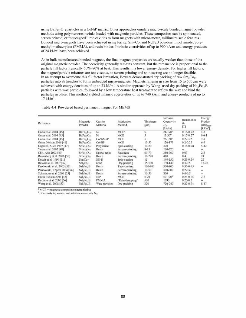
88

using BaFe12O19 particles in a CoNiP matrix. Other approaches emulate macro-scale bonded magnet powder methods using polymers/resins/inks loaded with magnetic particles. These composites can be spin coated, screen printed, or “squeegeed” into cavities to form magnets with micro-meter, millimetre scale features. Bonded micro-magnets have been achieved using ferrite, Sm–Co, and NdFeB powders in polyimide, poly-methyl methacrylate (PMMA), and resin binder. Intrinsic coercivities of up to 900 kA/m and energy products of 24 kJ/m3 have been achieved.

As in bulk manufactured bonded magnets, the final magnet properties are usually weaker than those of the original magnetic powder. The coercivity generally remains constant, but the remanence is proportional to the particle fill factor, typically 60%–80% at best. This results in a lower energy density. For higher fill factors, the magnet/particle mixtures are too viscous, so screen printing and spin casting are no longer feasible. In an attempt to overcome this fill factor limitation, Bowers demonstrated dry packing of raw Sm2Co17 particles into Si trenches to form embedded micro-magnets. Magnets ranging in size from 15 to 500 µm were achieved with energy densities of up to 23 kJ/m3. A similar approach by Wang used dry packing of Nd2Fe14B particles with wax particles, followed by a low temperature heat treatment to reflow the wax and bind the particles in place. This method yielded intrinsic coercivities of up to 740 kA/m and energy products of up to 17 kJ/m3.

Table 4.4 Powdered based permanent magnet For MEMS

89

BIBLIOGRAPHY

1. T.J.E Miller: Brushless Permanent Magnet and Reluctance Motor Drives, chapter 3.

2. D.Hadfield: Permanent Magnet &Magnetism: theory, materials, design, manufacture and applications, chapter 11,12.

3. Rollin J. Parker: Advances in Permanent Magnetism, chapter 5.

4. Roberto C. O’Handely: Modern Magnetic Materials Principles and Applications, chapter 13.

5. David P. Arnold, Member, IEEE, and Naigang Wang, Student Member, IEEE Journal of Microelectromechanical Systems . volume 18, issue no. 6, page 1255,Dec. 2009.

6. Hanne Jussila, Pia Salminen, Asko Parviainen*, Janne Nerg and Juha Pyrhönen, Proceedings of the 2008 International Conference on Electrical Machines, paper ID 1113.

7. Zhuonan Wang, Yuji Enomoto, Motoya Ito, Ryoso Masaki, Shigeki Morinaga, Hiromitsu Itabashi, and Shigeho Tanigawa, IEEE Transaction on Magnetic , volume 46, issue no. 2, Feb. 2010. 8. Bo Zhang and Gareth P. Hatch, IEEE Transactions on Magnetic, volume 45, issue no. 10, oct.2009.

9. Chun Li and Michael Devine, IEEE Transactions on Magnatics, volume 45, issue no.10 , Oct.2009.

90

CHAPTER 5

“APPEDIX”

PROPERTIES OF OLD MATERIALS FOR

PERMAET MAGET

91

Introduction

There are different parameters and properties for permanent magnet therefore, it is essential to make classification for the permanent magnet materials . There are many methods for classifications , but the most useful one is to divide them into groups each of which consists of members associated in some respect. The system used resolves the field into the following groups and is based mainly on composition and structural features: I Martensitic or quench-hardened steels II Dispersion-hardened alloys III Work-hardened alloys IV Order-hardened or super-lattice-forming alloys V Metallic powders, self-bonded VI Metallic powders bonded with a bonding agent VII Ceramic powders , self- bonded VIII Ceramic powders bonded with a bonding agent IX Miscellaneous It is used to refer to materials suitable for permanent magnet manufacture as “magnetically hard” materials; the groups listed are distinguished mainly by the processes employed to confer magnetic hardness on the group members and by the means whereby actual magnets are formed and held together as geometrical solids suitable for incorporation in apparatus or technical devices. If coercivity is regarded as the most important single property of a permanent magnet materials, a certain degree of classification can be made on the basis of the means adopted to develop this essentially structure property. They include mechanical strain, developing ferromagnetic anisotropy in a suitable phase and combining non-ferromagnetic elements with an element such as manganese.

92

GROUP I MARTESITIC OR QUECH-HARDEED

STEELS

93

5.1. Adding elements to steel The usual methods of steel manufacture involve melting, refining and carburization; in consequence, elements other than iron and carbon find their way into the finished steel from the raw materials and the furnace lining. It is customary to designate these elements as harmful, neutral or benign. These classifications are relative, because they really require reference to some specific range or proportion beyond which the element concerned cannot be tolerated. For example, small quantities of “benign” elements may be added to an alloy to effect de-oxidation or to confer hot working properties but even these elements can have undesirable effect when present in excess .The modifications of magnetic properties brought by adding limited amounts of certain elements to three widely used types of permanent magnet alloys are reported in Table 5.1.

5.2. Iron and carbon

Iron is one of the transition elements, it has atomic number 26 and atomic weight 55.85. It has a density of 7.868gm/cm3 and the melting point is 1,535oC. It is ferromagnetic in a certain temperature range and exists in various temperature-dependent allotropic modifications. In traversing the range from ambient or “room” temperature to the melting point, the allotropic forms are α, with a body-centred cubic (b.c.c.) Fig. 5.2(a) crystal

structure; ᵧ which has a face-centred cubic(f.c.c.) Fig.5.3(b) structure and , which reverts to the former body-

centred cubic structure. The α-structure is stable from room temperature to 910oC; it ceases to be ferromagnetic at temperature above 770oC, but there is no alteration in crystal structure accompanying this change.

The ᵧ-structure is stable between 910o and 1,403oC and -structure exists between 1,403oC and the melting point

1,535oC. The two b.c.c. structures are usually distinguished by the titles α-ferrite and ferrite and the f.c.c. structure is termed austenite. Iron in the α-form has the highest saturation magnetization at 20oC (Jsweber/meter2 [4πJs gauss]) of all elements. Carbon also exists in allotropic modifications; it has atomic number 6 and atomic weight 12.01, the density of carbon is 3.508gm/cm3 for the diamond and 2.265 for graphite. Carbon is sparingly soluble (as a solid solution) in

α- or ferrite (not more than about 0.04%) but can be taken into solution in ᵧ-iron(austenite) to the extent of

about 1.7%. Table 5.1 The effect of the addition of small quantities of certain impurity elements to three widely used types of anisotropic permanent magnet alloys.

94

Table 5.1 (cont.) The effect of the addition of small quantities of certain impurity elements to three widely-used types of anisotropic permanent magnet alloys of remanence , (BH)max and coercivity

Fig.5.1 (a) Body-centred cubic structure-typical of ferrite or α-iron.

(b) Face-centred cubic structure-typical of austenite or ᵧ-iron.

5.3 Steel

The fabrication of steel includes many operations such that refining, carburizing and de-oxidation and requires the exercise of much skill and knowledge. Suppose that such a series of operations has resulted in the production of some steel containing 0.30% of carbon and that steel has been cast into a mould. If a sample of cold casting is re-heated to a temperature in excess of 910 oC , the ferrite becomes transformed into

ᵧ-iron or austenite. As austenite can take much more carbon into solution than ferrite, a new and unstable situation

will exist until all the carbon present as cementite is dissolved and the sample becomes a homogeneous mass of austenite. Slow cooling by leaving the reheated sample to cool down in the furnace after switching off, produces an annealed structure consisting of ferrite and pearlite, annealed Steel containing 0.16, 0.30 and 0.45% carbon. When the carbon content reaches 0.82-0.83%, the structure is completely pearlite.

5.4. Heating and cooling In the fabrication of metallic magnets, they may be heated, held at a temperature or cooled. Variations in the heating rate, holding time and cooling can be made separately or in combination, magnet can be heated very rapidly throughout its mass, for example, by passing a heavy electric current through it. In cooling, however, the disposable heat must be extracted through the outer surface. The rate of cooling, therefore, depends on exo- or

95

endothermic changes in the specimen, its specific heat, its initial temperature, its thermal conductivity, the relation between cross section and surface, the size of the specimen and the overall heat transfer coefficient between the metal and the cooling medium. The total effect is such that, with bars greater than a few square inches in cross sectional area, the central or axial portion can never be lowered in temperature at a sufficiently fast rate to develop desirable magnetic properties. A top limit of section is imposed, therefore, on individual permanent magnets subject to rapid quench.

5.5. Changes on heating and cooling

Principally, a magnet is heated to a temperature sufficient to permit one constituent to pass into solid solution with another. Such processes are sometimes sluggish, so a certain holding time may be necessary once a given temperature is reached. From this point of view, successive treatment is designed to introduce a high degree of heterogeneity or other structural mismatch into the magnet because such conditions have been found to be associated with good permanent magnet properties. With plain carbon steel, the treatment involves quenching in water or oil.

5.6.Annealing To fabricate magnet from magnet steels, operations like stamping, machining and drilling are used. For these processes, mechanical softness in the work piece is required, it is obtained by annealing so that a pearlite structure will be produced. Machinability and high remanence characterize magnet steels and, for some applications outweigh their low coercivity. Sustained annealing is sufficiently prolonged to cause the carbides to ball-up (spheroidizing) and transformation treatment.

5.7. Magnetic properties of carbon steels 5.7.1. Low carbon steel

Such material is being used in the yokes and fields of direct current generators of the self-exciting type, for example, motor-car and train-lighting dynamos. These machines depend upon remanent magnetism in the yoke to ensure a build up of voltage when starting from rest. The remanence of the field material is of the order of 0-700 weber/meter2 but the coercivity rarely exceeds 80 to 120 ampere turns/meter . 5.7.2. Medium to high carbon steel

As experience has proved that magnetic hardness of plain carbon steels is closely associated with physical hardness, it is natural to induce the highest possible hardness in carbon steel magnets by quenching to produce the martensitic structure. By taking a series of steels with a range of carbon contents from less than 0.1% up to about 1.8% and quenching for maximum hardness, it is possible to follow the change in permanent magnet properties that accompany change in carbon content. Fig.5.2 shows the relation between remanence, coercivity and (Brem × Hc ) and the carbon content of a series of such steels.

Fig.5.2 Magnetic properties of hardened carbon steel for the range of carbon contents up to 1.5 per cent.

96

5.7.3. Permanent magnet behaviour

At least two essential qualities are necessary in a material so that it may function as a permanent magnet. First, it must be possible to induce a very high degree of magnetization in it by the application of a sufficiently strong magnetic field, i.e. the material must have a high saturation intensity(Js weber/meter2 ). Second, a large part of the magnetization thus induced must be locked in by some structural heterogeneity that opposes a return to the unmagnetized condition. Martensite exhibits the type of heterogeneity necessary for this second condition, so it is to be expected that increases in the carbon content ( by increasing the number of solute atoms to be accommodated in the tetragonal structure) will increase the strain therein and be associated with an increase in coercivity. Such increase in carbon content however, is accompanied by a decrease in saturation intensity, thereby opposing the first requirement namely, the induction of a high degree of magnetization. Fig.5.2 shows these effects; the coercivity increases in a linear manner with the carbon content up to about 0.8%. The rate of increase falls off with higher carbon content and at about 1.8% this rate is practically zero. As the coercivity increases, the remanence falls but the fall is arrested at a content of about 1.1% . The (Brem×Hc) graph reaches a maximum at about 0.8% carbon (i.e. practically at the eutectoid composition). It is possible that a steel made with iron and carbon of a very order of purity might have exceptional magnetic properties; commercial steels however, contain the usual impurities and residual elements associated with the steel making process. With such steels, it has been found that a carbon content between 0.9 and 1.0% gives a permanent magnet that satisfies practical applications for which a remanence of 0.95-1-0 Weber/meter2 and coercivity of 4,000 ampere turns/meter2 are acceptable. The (BH)max of such material is about 1,600 joules/meter3, see Fig. 5.3.

Fig.5.3. Demagnetization curve of 0.9 per cent carbon steel

5.8 Alloy magnet steels

It appears that some improvement in permanent magnet properties might be secured by the addition of hardening elements that would favour enhanced values of Hc without causing the severe falling off in Brem that accompanies increase of carbon in plain carbon steel. Suitable elements are tungsten, chromium and cobalt; alloy magnet steels that containing these elements, display much better magnetic properties than plain carbon steel. The compositions and magnetic properties of these alloys are given Table5.2.

97

Table5.2 Magnet steel and alloy steels

Table 5.2 (cont.) Magnet steel and alloy steels

98

Table 5.2.(cont.) Magnet steel and alloy steels

5.8.1 Hardening

The alloy magnet steels are all hardened by quenching and in general, the heterogeneity necessary for permanent magnet properties is enhanced by the reaction of a proportion of austenite in the structure. The action of the alloying elements in this respect is comparable with a much increased quenching rate on a plain steel; therefore the austenite does not has sufficient time to transform completely into martensite. In the extreme, steels containing for example 18% chromium and 8% nickel or 13% manganese and 1% carbon have the transformation characteristics so modified that on quenching from solution temperature, an entirely austenitic structure is retained; in this condition, the materials have negligible magnetic properties.

Spoiling . The alloying elements combine to form massive carbides with some of the carbon in the alloy magnet steels if the temperature is held for long in the range 950-1,000oC for example, during forgoing or rolling consequently the materials may be brought into a condition from which the normal magnetic properties cannot be developed on hardening. This phenomena is termed “spoiling”. It is possible to reclaim such spoiled material by a subsequent solution or austenizing treatment at 1,200oC before the final hardening. The furnace atmosphere and other conditions require careful control. With some of the alloy magnet steels, for example the cobalt series, the high temperature solution treatment forms part of the normal manufacturing sequence.

Tempering. After hardening the stability of some of the magnet steels can be improved, at the cost of slight impairment of the magnetic properties, by immersion in a water or oil bath controlled in the temperature range 90-100oC for periods up to 10 minutes. Manufacturing methods. All the alloy magnet steels can be forged, rolled or cast to shape and most machining operations can be undertaken if the material is in the annealed condition. The manufacturing operations are attended with great difficulties as the alloy content increases; among other characteristics, an increasing proportion of alloying elements brings increased brittleness. Range of Magnetic Properties. Compared with plain carbon steel, the magnetic properties of the alloy magnet steels in terms of (BH)max range from those of 2.5% chromium steel, which is roughly 25% better than plain carbon steel, to those of 40% cobalt steel which is about five minutes as good as the plain steel. 5.8.2 Alloying elements

Chromium: Chromium has atomic number 24 and atomic weight 52.01. It has a density of 7.1gm/cm3 and the melting point is 1,920oC . It is paramagnetic with a mass susceptibility of 3.08×10-6 emu per gram. It is used as an alloying element in its own right for a series of magnet steels nominally containing 2.5, 4.0 and 6.0% chromium. It also serves as a subsidiary alloying element in most of the alloy magnet steels. Chromium slows down the rate at which austenite transforms at any particular temperature. In consequences, a thicker section can be hardened throughout in chromium steels than is possible with plain carbon steels. Chromium, like tungsten and molybdenum, is classed as a carbide-forming element. Tungsten. Tungsten has atomic number 74 and atomic weight 183.92. It has a density of 19.32gm/cm3 and the melting point is 3,382oC . It is paramagnetic with a mass susceptibility of 0.82×10-6 emu per gram. It is used in the

99

well-known 6% tungsten magnet steel in combination with 0.7% carbon, from 0.3 to 0.9% chromium and up to 0.5% cobalt. As a subsidiary alloying element it is incorporated in most of the cobalt series of magnet steels, depending on the manufacture, in amounts up to 8%. The maximum quantity of tungsten that can be taken into solid solution in iron is about 6% at 1,200oC . When used as alloying element in steel, tungsten has a similar effect to chromium; it has a retarding effect on the critical cooling rate and also, therefore, promotes better depth hardening. A further effect of tungsten is that it slows down the solution of carbides; the soaking time for solution treatment, therefore, it has to be adjusted accordingly. Cobalt. Cobalt has atomic number 27 and atomic weight 58.94. It has a density of 8.71 gm/cm3 and the melting point is 1,478oC. Unlike the two elements previously mentioned, cobalt is ferromagnetic with a curie point at 1,121oC; when alloyed with iron, it increases the saturation magnetization. A saturation value of Js equal to about 2.4 webers/meter2 is reached with an alloy containing 33% cobalt. Cobalt also increases the rate of diffusivity of carbon in gamma iron at 1,000oC and induces very high magneto-striction in iron-cobalt alloys. Cobalt is used in proportions ranging from the 0.5% ( used in the 6% tungsten steel) to the 40% used in the cobalt steel (40%CO,5%W,5%Cr,0.7%C) which is note worthy as a magnet steel with an energy product (BH)max of 8,000 joules/metre3

.

Aluminium. Aluminium is an important constituent of permanent magnet alloys. Apart from its use as a de-oxide, however, little use is made of aluminium in magnet steels. It is an element of atomic number 13 and atomic weight 26.98. it has a density of 2.7 gm/cm3 and the melting point is 660oC. It is paramagnetic with a mass susceptibility of 0.65×10-6 emu per gram.

100

GROUP II DISPERSIO-HARDEED ALLOYS

101

This group contains several sub-groups; it also includes the most important of the high energy magnetic alloy. Some of the group members do not include iron in their composition; in all of them carbon is an undesirable constituent. Most of the commercial alloys in the high energy class contain several elements. For example, aluminium, cobalt, copper, iron, niobium or titanium and sometimes silicon are listed as important constituents in one series of alloys, apart from residual or trace elements; the study of such alloys is, in consequence, very complex. It is possible, however, to separate the group members into at least three main types depending on the metallurgical background to the dispersion hardening process applicable to individual members. Dispersion hardening in an alloy can be envisaged as hardening consequent upon a type of change that occurs on an individually minute scale but at a vast multitude of points throughout the mass of the alloy. Precipitation phenomena can be considered as involving coarse-textured dispersions.

5.9. Single precipitation

The simplest illustration of the first main type is the single precipitation or age-hardening that occurs in some low carbon steels. A steel containing about 0.04% carbon will, when re-heated to 700oC and cooled rapidly to room temperature, retain carbide in solid solution (Fig. 5.4). Subsequently, while the steel is still at room temperature, the carbide is precipitated in exceedingly fine particles throughout the material and the hardness of the latter is increased.

Fig.5.4 Precipitation phenomena in low-carbon steel

5.10. Binary alloy

By examining the equilibrium diagrams of binary alloy other iron containing systems can be found in which precipitation occurs from supersaturated solid solution, after appropriate heat treatment. Among such systems are iron-beryllium, iron-molybdenum, iron-titanium and iron-tungsten. The iron-molybdenum system is of particular interest and has been subjected to close study by Sucksmith and Margresion who have shown, for example, that if an alloy containing between 10 and 20% Mo, balance Fe, is heated to the solution temperature say 1,300oC and then quenched, the single phase structure is retained.

On ageing by re-heating and holding in the range 550-700oC , however, the non-magnetic phase, Fe3Mo2 , is precipitated in platelet form, the number and disposition of the platelets being such that the ferromagnetic matrix is divided into zones of the right order of magnitude to constitute single domains and so to confer useful permanent properties on the material. Evidence with respect to the existence of the precipitates (that are such an important feature of permanent magnet alloys) has to be obtained by indirect means because the individual particles of the precipitates are usually of such minute dimensions that ordinary microscopic techniques are inadequate to reveal them.

102

The indirect methods that are used include re-heating to higher temperatures and/or for longer periods than would normally be used in the ageing or tempering process so that the precipitates nucleate or grow to detectable proportions. The structure noted then is really that a specimen that is “spoiled” in the magnetic sense. By using electron microscope techniques, the amount of spoiling can be kept to a minimum and a representation of the structure that is probably very near to that of a correctly heat-treated alloy is obtained. It is quite possible that, in some instances, the best magnetic properties are developed at some stage, e.g. of partial atomic re-arrangement, that immediately precedes the onset of precipitation. Precipitation processes can also be operated with the other binary alloys mentioned and the available information with respect to them is reported in Table 5.3.

Table5.3 Precipitation-Hardening binary iron alloys

5.11.Ternary alloy

Several ternary alloys have been developed with similar precipitation-hardening properties to the binary alloys just mentioned. A representative composition is 17% Mo,12%Co, and balance Fe (Comalloy). This material is solution treated by heating to a temperature in the range 1,200-1,300 oC and is quenched in oil. After quenching, the material is aged by reheating to 685-700oC and holding at temperature for 1½ hours. During this ageing process, a

complex derived from the compounds Fe3Mo2 (Ԑ-phase in the iron-molybdenum system) and CoMo (ᵧ-phase in

the cobalt-molybdenum system) precipitates in a ferrite solid solution.

The material can be cast or forged and, since its magnetic properties are similar to most 35% cobalt steels, it can serve as substitute for the latter when there is need to economize in cobalt for cost or other reasons.

Some workers have reported a practical drawback in that cross-sectional areas greater than about 2 cm square cannot be satisfactorily heat treated on account of mass effect. There is also a reported tendency to spall at edges and corners that adds to manufacturing difficulties. Work on this alloy in Great Britain has shown, however, that some of the difficulties can be overcome by care in choosing the working range of composition and also by incorporating additional alloying elements. As an example of the latter approach, an ingot containing 12.15% Co,16.6% Mo,0.77% Mn , and 0.44% Ti.

5.12. Double precipitation or co-precipitation

The second main type of dispersion-hardened alloy can be illustrated by the iron-nickel-copper system which introduces two elements that have not figured in the permanent magnet that was mentioned previously. In order of atomic numbers they are nickel 28 and copper 29 with respective atomic weight 58.69 and 63.54. The densities are

103

nickel 8.9 and copper 8.69gm/cm3 . The melting points are 1,455oC for nickel and 1,083oC for copper. Nickel like iron and cobalt, is ferromagnetic with curie point 358oC. It forms a series of alloys with iron that are of great importance both magnetically and otherwise. Copper is diamagnetic with mass susceptibility of 0.086×10-6 emu per gram and has a limit of solid solubility in iron of about 2%. Iron-Copper alloys containing more than about 2% copper have a two phase structure and exhibit an increase in coercivity and a decrease in saturation intensity as the copper content increases. Since increase in coercivity is tantamount to increase in magnetic hardness and the iron-copper alloys are not mechanically hard, they form an important departure from the correspondence between magnetic and mechanical hardness that is usually characteristic of magnet steels.

The alloys of copper and nickel are single phase for all proportions from 100% Cu to 100%Ni and show no appreciable magnetic properties for nickel content less than about 65%. The constitution of the ternary alloys of iron, nickel and copper is shown by the diagram Fig.5.5, in which the third element is accommodated by making the diagram in the form of an equilateral triangle. It is important to observe that ternary diagram can only display the state of the system concerned at one particular temperature and, further, this state may or may not be done of true equilibrium. Constitutional diagrams may be drawn in terms of either weight or atomic percentages. The latter scale is more usual in scientific work. Since the relation is not linear between the two scales, a diagram drawn in terms of atomic percent of given elements may appear distorted in comparison with one for weight percent of the same elements; it is, however, more convenient for fixing the position of compounds that have a definite chemical formula. The full lines in the figure show the phase boundaries corresponding to alloys slowly cooled to room temperature. The broken line shows the modification of the boundary ABCDEF that takes place when the reference temperature of the system is raised to1,050oC .

The region to the right of the broken line includes a range of compositions that might roughly be described as 20%Ni, x% Fe and y% Cu where x + y=80. Practically all the compositions in this range have face-centred cubic

ᵧ-structure but there is some difference in unit cell dimensions or lattice parameters in passing from ᵧ1(copper-rich)

to the ᵧ2(iron-rich) part of the diagram. At the solution temperature of 1,050 oC, these differences are

accommodated and a single ᵧ-phase exists.

A composition like 20% Fe, 20% Ni and 60% Cu is ingle-phase at the solution temperature but, as it lies to the left

of ABCDEF, consists of a mixture of ᵧ1 and ᵧ2 when slowly cooled to room temperature. If , however, it is cooled

rapidly by quenching, the separation into ᵧ1 and ᵧ2 is inhibited and a supersaturated solid solution of one in the other results.

104

Fig.5.5 The Cu-Ni-Fe diagram

5.13. The Alni sub-group.

The range of possible alloys of iron, nickel and aluminium has been critically explored and the diagram of Fig. 5.6 shows the fields of interest. Certain compositions have been marked on this diagram, namely the 30% Ni, 12% Al, balance Fe alloy. It has been established by experiment that when the typical alloy of this class is raised to a high temperature 1,100oC, it is in a state of single-phase solid solution and also, that when it is cooled rapidly from this temperature, an important change takes place in the short interval (about 3 seconds) during which the alloy passes through the range 900-800 oC. The cooling rate is too fast for equilibrium condition to be approached and it appears the magnetic hardening induced by this simple heat treatment. At high temperature, the alloy exists as a body-centred cubic phase; the two low temperature phases are also body-centred cubic but there is a slight mismatching to extent of about 1% in the lattice parameter.

105

Fig.5.6 Controlled Cooling of FeNiAl alloy and corresponding magnetic properties.

However, in a correctly heat treated magnet there is no question of the separate appearance of these phases even on the smallest scale. Bradely and Tylor, and Burgess and Snoek have shown that slight broadening of the 310 reflection obtained by X-ray diffraction techniques corresponds to material of the Fe2NiAl type heat treated for maximum coercivity. Such slight broadening is not consistent with separation of the phases. It may be that the postulated atomic diffusion process responsible for magnetic hardness occurs as a three dimensional analogue of a moiré fringe or interference pattern throughout any given small portion or zone of the material, the gradual nature of the pattern variation is being such that there is no great modification of the X-ray diffraction pattern for example, with super lattice formation.

A useful feature of Alni alloys is the possibility of adjusting the magnetic performance by altering the nickel content. Thus an alloy with 21% Ni, 13% Al and balance Fe has a remanence of 0.78%weber/meter2 and a coercivity of 20,800 ampere turns/meter. An alloy containing 27% Ni,13% Al and balance Fe has a lower remanence at 0.58 Weber/meter2 but nearly double coercivity at 40,000 ampere turns/meter. The energy product (BH)max is the same for both alloys at 8,800 joules/meter3. The ability to adjust performance so readily, helps to ensure that a given design of instrument or other device is served in the most efficient matter by the magnet incorporated in it; particularly where space considerations preclude any significant alteration of dimensions.

The optimum composition for a given purpose, once determined, should be closely adhered to in the melting process. A reduction of 1% in the aluminium content, for example, can bring about a 40-50% drop in coercivity and 35-40% fall in (BH)max energy product. Carbon, although an essential constituent of magnet steels, should be kept as low as possible in Alni type alloys. Tests have shown that Alni with a carbon content of 0.12% gives a (BH)max energy product that is about 20% lower than (BH)max figure of practically carbon-free Alni.

Titanium, with atomic number 22, has atomic weight 47.90 and density 4.5gm/cm3. Although such a light metal, it has a melting point that at 1,690oC is higher than that of iron. It is paramagnetic with mass susceptibility of 1.25×10-6 emu per gram. It has a pronounced grain-refining effect in alloys and enhances coercivity by forming titanides of iron, cobalt and nickel. Niobium, also known as columbium, has atomic number 41, atomic weight 92.91 and density 8.4 gm/cm3. The melting point is high at 2,500oC. It is paramagnetic with mass susceptibility of 1.5×10-6 emu per gram. Once considered a rare metal, niobium has now become of wide technical importance.

106

5.14. The Alnico sub-group

The improvement in magnetic properties consequent upon the addition of copper to the Alni type alloy stimulated the investigation of other alloy additions, particularly cobalt. The successful outcome of this investigation was established of the largest class of commercially used permanent magnet alloys that containing cobalt in proportions ranging from 5 to about 35%. The application of the word “Alnico” is wider in some countries than others; this point is brought out in tables.

The Alnico sub-group can be divided as follows:-

1- Isotropic materials in which the magnetic properties are practically identical when measured along axes chosen at random in the material.

2- Anisotropic materials have a preferred magnetic axis or favourable direction of magnetization established in the material by placing it in a strong magnetic field, aligned with preferred direction, while it is cooling at a controlled rate after being heated to the hardening temperature. Such materials have the magnetic properties enhanced along the preferred axis and reduced along any other axes at right angles to it. By cooling in a radial field, it is possible to produce a magnet that has its properties reduced along one axis and enhanced along any other axes at right angles of it.

3- Anisotropic materials have a structurally (i.e. crystal-graphically) favourable direction in addition to, and in alignment with, the preferred magnetic axis that was mentioned above. This physical process of directional solidification, adjusted by suitable arrangements of heat sources and sinks, is used to produce a favourable alignment of the crystal structure, for example, by growing columnar crystals in a desired direction. In this way, advantage may be taken of crystal anisotropy by combining a magnetically crystal-graphic direction, i.e. an easy direction of magnetization with the preferred magnetic direction subsequently produced by controlling cooling in a magnetic field. The highest value of maximum energy product so far reported has been measured on a magnet of this third type.

5.15. The isotropic Alnico type alloys

The isotropic alnico type materials, like the Alni class, can also be produced with a range of properties to suit particular applications; in consequence, there is a fairly extensive spread in composition as will be apparent from the range given in Table 5.4.

5.15.1. Composition range

It is fairly simple matter to imagine the extension of the iron-aluminium-nickel triangular diagram Fig.5.7 in a direction perpendicular to its plane, by superimposing a number of isotherms corresponding to the constitution at progressively higher temperatures. In the lamina representing 1,200oC it would be found, for example, the composition Fe2NiAl is a single phase solid solution represented by a point located vertically above which on the base or room temperature lamina, corresponds to a two phase structure.

With the addition of fourth element, e.g. cobalt to the iron-aluminium-nickel system, the constitution at any given temperature can no longer be represented by a plane triangle; a solid figure or space diagram with four equilateral triangles as faces; i.e. a tetrahedron, is necessary. Instead of using triangular lamina to represent the constitution at particular temperatures, a complete tetrahedron must be constructed anew for every level of temperature and can show permanent magnet properties when approximately heat treated; the desired properties of high coercivity or high remanence are determined, within limits, by adjusting the alloy proportions as with the Alni series.

107

Table 5.4 the isotropic “Alnico” class

Table 5.4 (cont.) the isotropic “Alnico” class

108

Table 5.4 (cont.) the isotropic “Alnico” class

5.15.2. Effect of extra alloying elements in alnico alloys

When cobalt added to the iron-aluminium-nickel, the system tends to slow down the diffusion process as represented by the curve in Fig.5.6 so that instead of a cooling rate approximating to 30oC per second, about one tenth of this rate suffices for alloys with suitable cobalt addition. This effect may be likened to that of adding chromium to plain carbon steel that has been discussed previously.

Addition of cobalt, therefore, increase the permissible size of cross section and allows the sturdiness castings in Alnico. The influence of cobalt in developing a structure favourable to permanent magnet properties is supplemented by its capacity for increasing the magnetic striction and the saturation inducing; moreover the curie temperature of the alloy is progressively raised as the cobalt content is increased so that useful enhancement of the magnetic properties by magnetic field treatment at high temperatures is facilitated.

Copper can be classed to a limited degree with cobalt, in respect of its effect on the iron-aluminium-nickel system, as it slows down the diffusion process and also, when present with cobalt, enhances the beneficial effects of the latter and improves coercivity. To some extent, it is of service in minimizing the effects of slight composition variations thereby favouring good reproducibility of magnetic test results .

Titanium has already been mentioned as an alloying element in Alni types alloys to the extent of 0.4%. In the Alnico series, massive additions of titanium, up to 11% have been made. Alloys of this extreme composition have very high coercivity but are even more brittle than ordinary Alnico alloys.

The Alnico class may be simplified into a few main types with a composition of 10-12% Al, 15-20% Ni, 5-14% Co and 0.6% Cu. The typical heat treatment sequence commences with reheating to 1,200-1,250oC and cooling at a controlled rate.

A typical composition range for the titanium bearing alloys developed at the same time as Alnico is aluminium little or none, 10-20% Ni, 10-30% Co, 10-11% Ti. This type of alloy and its near relatives have magnetic properties in the range remanence 0.5-0.6 weber/meter2 , coercivity 60,000-80,000 ampere turns/meter and energy product 12,800-16,000 joules/meter3 .

109

GROUPIII WORK HARDEED ALLOYS

110

Most materials in the pure or nearly pure state are ductile and can be deformed by cold work. The term ”cold” is relative; metals can reach high local temperatures during cold rolling or wire drawing. The character of the deformation can be random as in crumpling a piece of metal foil or rectangular as in wire drawing or in rolling strip or sheet metal. In an individual crystal the permanent or plastic deformation may start at a very low loading, the manner of the yield being in very small but distinct steps each of which involves a shearing of the crystal along certain preferred or “glide” planes. The point of interest in respect of cold working is the fact that materials normally having weak or even negligible magnetic properties can, after suitable mechanical deformation, exhibit useful magnetic properties comparable with conventional permanent magnets. The mechanical stresses induce strains (i.e. extension or compression) and impose restraints that interact with magnetic striction normally operating in the presence of a magnetic field. Two common methods of cold reduction, will be examined, first, cold rolling strip or sheet material and, secondly, drawing through dies to produce wire. Strip. The material of the original slab is elongated without any appreciable alteration in its width and the extent of the elongation can easily be 100 times or more. If, therefore, a given direction makes angle α, of tangent t with a line of cross section in the original material then, after rolling, the direction will make a new angle of tangent 100t with the cross section. If α is more than a few degrees, then the new angle will be practically 90 degrees. The consequence is that all lines, planes and boundaries are swung round, in the course of rolling, so that they are practically parallel with the longitudinal axis of the strip. A pronounced anisotropy of structure is produced, therefore, apart from any metallurgical changes that may take place. Wire. In wire drawing, the finished length may easily be 1,000 times that of the original wire bar, but the mechanism or deformation is different from that obtaining in strip rolling. The action of the wire drawing is not die uniform across the cross-section of the wire; an original plane cross-section tends to become part of a parabolic. There is also a difference between wire continuously drawn down in one direction by passing through a succession of dies in a multi-pass machine and wire that has a reversal at each pass. With both strip and wire there are usually numbers of annealing necessary in the course of reaching finished size, the properties of the finished material are particularly influenced by the amount of reduction after the final anneal. Once finished size is reached, it is possible to make some modification of magnetic properties by further heat treatment. This can be beneficial to permanent magnet properties up to a particular combination of time and temperature, but if these optimum conditions are overshot, the material may be spoilt without chance of reclaim except by drawing down at a smaller size. For present purposes, only cold deformation of alloy materials will be considered. It has been seen that in this process, extreme pressures are exerted on the material and gliding is forced to take place in a great number of planes simultaneously. If the alloy is in a metastable condition at room temperature, as in the instance of some austenite, there is a strong possibility that the deformation will lead to separation into two or more phases including at least one magnetic and one non-magnetic phase distributed through the structure in an array similar to those produced in dispersion-hardened alloys by suitable heat treatment. Other types of stability temperature relations may operate, e.g. a phase stable at room temperature where the co-existence of two phases is favoured . If the phase change is made sluggish by suitable choice of alloys, the tempering process can be slow enough to permit effective development of optimum magnetic properties. The types of alloys particularly suited to development of magnetic properties in cold-worked material may be grouped as follows: 1.Austentic alloys, based on high nickel and chromium or high manganese content. 2.Vicalloy type, based on the iron-cobalt-vanadium system. 3.Cunife and Cunico types, based on the copper-nickel-iron and copper-nickel-cobalt systems. 4.Silmanal type, based on the manganese-silver-aluminium

5.16 Austenitic alloys stainless steel.

Two well known alloys in this class are 18/8 and 12/12 chromium-nickel compositions. In alloys made from high-purity raw materials, both compositions are on the borderline of stability in respect of being fully austenitic at

111

room temperature. The impurities normally present in commercial steels, notable nitrogen, have a stabilizing influence on the austenitic structure, and inhibit spontaneous separation of a body-centred cubic ferrite phase. This separation does occur in the course of cold working by some mechanism of the type already described.

Of the two alloys, more use for magnetic purposes has been made of the12/12 type than of the 18/8 type; both have been used to produce wire of about 0.004 inch diameter for use in sound recording. It is possible to reach remanence figures of about 0.6 weber/meter2 with coercivity up to 16,000 ampere turns/meter in the hard drawn wire, and some improvements in properties can be secured by a tempering treatment.

5.16.1 High-Manganese steel

The well known 12-14% Mn, 1% C steel is used for conditions of heavy service, e.g. mechanical digger teeth, and can exhibit a high degree of work hardening in such use.

The work hardening of manganese steel has been attributed in the past to the formation of martensite, but recent work has shown that the hardening by deformation can be attributed to the formation of a hexagonal phase in a face-centred cubic matrix. In order to examine the possible causes more fully, a series of samples of 13% manganese steel was prepared using as nearly pure materials as were available. The carbon contents ranged from 1.0% to the lowest attainable. The deformation was applied by taking a small cylinder of the material and hammering it flat on a hard steel anvil. After deformation, the samples were examined by means of an electron microscope.

The samples with 1.0% C were deformed at temperatures ranging from room temperatures down to -196oC but no martensite was found. Samples with progressively smaller carbon contents tested in a similar manner: the first to show a trace of martensite when deformed at -196oC contained 0.7% carbon. With smaller carbon contents, the temperature at which martensite could be produced by cold deformation rose. The sample that just showed a trace of martensite when deformed at room temperature contained 0.3% carbon.

The advantages of these alloys are their comparatively high remanence and relatively low cost.

5.17 Vicalloy type alloys

All the elements in the series of atomic numbers 22 to 28 have so far been mentioned in some detail as useful alloying elements for permanent magnets with the exception of vanadium, atomic number 23. This element has atomic weight 50.95 and density 6.0 gm/cm3. It melts at 1,730oC and is paramagnetic with mass susceptibility of

1.4×10-6 emu per gram. The iron-vanadium equilibrium diagram shows a ᵧ-loop extending to about 1.0%

vanadium. This loop has a heterogeneous boundary extending to about 1.1% vanadium in which the α- and ᵧ-phases are apparently in equilibrium. Alloys containing more than 1.1% vanadium exist as a solid solution of vanadium in body-centred cubic iron. The effect of vanadium on steels, in general, one of improvement, particularly in respect of mechanical properties.

Vicalloy I contains 38% Fe, 52% Co, 9.5% V. The corresponding percentages for vicalloy II are 34,52,and 14. In some commercial alloys, other elements, e.g. chromium, are added to replace part of the vanadium. The mechanism for producing structures capable of exhibiting useful permanent magnet properties is similar in both Vicalloy I and II, but is achieved by different routes. For Vicalloy I, cold rolling may be used as an intermediate process for convenience in producing a given size or shape but it is not essential. Vicalloy II depends on the cold rolling operation for inducing the formation of an α-phase which, in Vicalloy I, is brought about by quenching from high temperature.

The procedures with these alloys are as follows:

Vicalloy I: cast, heat treat by quenching in oil from 1,200oC ; manipulate to the desired shape or form by hot rolling, cold rolling or machining, age or temper at 600oC for 8 hours.

112

Vicalloy II: cast, manipulate to intermediate size by hot rolling, swaging, or other convenient method, to produce a form that can subsequently receive 90% or more cold reduction to produce the finished size, age as before 600oC for 8 hours. The maximum energy product of Vicalloy II can approach 28,000 joules/meter3 which is about 3 ½ times that attainable with Vicalloy I. The actual mechanism that produces permanent magnet properties in the Vicalloy types appears to be an ordering phenomenon more than the precipitation process.

5.18 Cunife and Cunico

Cunife is workable and may be heavily cold rolled to produce thin strip or tape. The usual compositions aimed at Cunife I with 20% Fe, 20% Ni and 60% Cu. Cunife II has 27.5% Fe, 20% Ni, 50% Cu and 2.5% Co. The alloy is cast into an ingot, after soaking at a temperature of 1,000oC to homogenize the structure; it is quenched and aged at 650oC. Cold working in stages to produce the finished size is followed by a final ageing at 650oC. An alternative procedure that gives somewhat better magnetic properties is to swage down the homogenized ingot about 90-95%, quench from 1,070oC, further cold reduce to finished size, age at 600oC . The ageing time should be between 1 and 10 hours depending on the working that has preceded it. Cunico I has the nominal composition 50% Cu, 215 Ni and 29% Co. The variant Cunico II has 35% Cu, 24% Ni, and 41% Co. After casting, the homogenizing treatment requires rather longer periods and higher temperatures than for Cunife. The cold reduction and ageing procedures follows, in general, a similar pattern to that of the Cunife alloys.

5.19 Silmanal

Silmanal is an alloy of 86.8% Ag, 8.8% Mn and 4.4% Al. It was the first that was prepared by potter who was experimenting with Heusler alloys. By substituting silver for the copper in this type of alloy, he found that optimum coercivity corresponded to a composition that can be approximately represented by Ag5MnAl.

The important feature of Silmanal is its very high coercive force which makes it useful in the manufacture of instruments for measuring magnetic fields.

113

GROUP IV ORDER-HARDEED OR SUPERLATTICE-

FORMIG ALLOYS

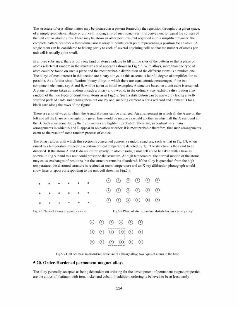
114

The structure of crystalline matter may be pictured as a pattern formed by the repetition throughout a given space, of a simple geometrical shape or unit cell. In diagrams of such structures, it is convenient to regard the corners of the unit cell as atomic sites. There may be atoms in other positions, but regarded in this simplified manner, the complete pattern becomes a three-dimensional array of points, each point representing a position for an atom. A single atom can be considered to belong partly to each of several adjoining cells so that the number of atoms per unit cell is usually quite small.

In a pure substance, there is only one kind of atom available to fill all the sites of the pattern so that a plane of atoms selected at random in the structure could appear as shown in Fig.5.5. With alloys, more than one type of atom could be found on such a plane and the most probable distribution of the different atoms is a random one. The alloys of most interest in this section are binary alloys, on this account, a helpful degree of simplification is possible. As a further simplification, binary alloys in which there are equal atomic percentages of the two component elements, say A and B, will be taken as initial examples. A structure based on a unit cube is assumed. A plane of atoms taken at random in such a binary alloy would, in the ordinary way, exhibit a distribution also random of the two types of constituent atoms as in Fig.5.8. Such a distribution can be arrived by taking a well-shuffled pack of cards and dealing them out one by one, marking element A for a red card and element B for a black card along the rows of the figure.

There are a lot of ways in which the A and B atoms can be arranged. An arrangement in which all the A are on the left and all the B are on the right of a given line would be unique as would another in which all the A surround all the B. Such arrangements, by their uniqueness are highly improbable. There are, in contrast very many arrangements in which A and B appear in no particular order; it is most probable therefore, that such arrangements occur as the result of some random process of choice.

The binary alloys with which this section is concerned possess a random structure, such as that in Fig.5.8, when raised to a temperature exceeding a certain critical temperature denoted by Tc . The structure is then said to be distorted. If the atoms A and B do not differ greatly, in atomic radii, a unit cell could be taken with a base as shown in Fig.5.9 and this unit could prescribe the structure. At high temperature, the normal motion of the atoms may cause exchanges of positions, but the structure remains disordered. If the alloy is quenched from the high temperature, the distorted structure is retained at room temperature and an X-ray diffraction photograph would show lines or spots corresponding to the unit cell shown in Fig.5.9.

Fig.5.7 Plane of atoms in a pure element Fig.5.8 Plane of atoms; random distribution in a binary alloy

Fig.5.9 Unit cell base in disordered structure of a binary alloy; two types of atoms in the base

5.20. Order-Hardened permanent magnet alloys

The alloy generally accepted as being dependent on ordering for the development of permanent magnet properties are the alloys of platinum with iron, nickel and cobalt. In addition, ordering is believed to be at least partly

115

responsible for the magnetic hardness of Vicalloy and Silmanal. It is possible that some of these difficulties may be overcome by using neutrons instead of X-ray. By the use of methods of a high degree of refinement, Petch was able to specify the positions of carbon atoms in face-centred cubic iron (austenite) and show that a super lattice exists in this structure. It is also probable that there is ordering in the martensite structure.

5.21. Platinum alloys

The platinum alloys are remarkable for very high coercivity. The platinum-cobalt alloy, in particular, can develop the highest value of maximum energy product of any known isotropic permanent magnet alloy. From the nature of the ordering process, it is to be expected that the development of optimum magnetic properties will be strongly dependent upon achieving the exact stoic metric composition; this expectation seems to be justified by practice.

Platinum and cobalt form a continuous series of solid solutions. At the 50:50 or equi-atomic composition the temperature Tc is 825oC; above Tc the alloy is distorted face-centred cubic; below Tc the structure is ordered face-centred tetragonal, with an axial ratio of 0.969 (Fig.5.10). The optimum heat treatment sequence for platinum-cobalt has been investigated by Martin and Geisler who report a maximum energy product of 71,500 joules/meter3

for nearly equi-atomic composition disordered by heating to 1,000oC and cooling from this temperature to 200oC in 10 minutes. After this, the material was partially ordered by ageing at 600oC for 5 hours.

Fig.5.10 Cobalt-platinum alloy CoPt; ordered and disordered structures.

A further improvement in the magnetic properties of platinum-cobalt is effected by the following heat treatment sequence. The material is distorted by heating to 950-1,000oC for a period of 3 hours. It is then transferred to a salt bath, maintained at 660oC for a further period of 15-45 minutes depending on the previous history and the precise composition of the material. Protection must be given against oxidation in the furnace and the transfer from furnace to salt bath must be made rapidly, so that temperature of the material does not fall below 660oC.

5.22 Vicalloy-type alloys

Cobalt-vanadium-iron alloys have been mentioned in previous sections. Vicalloy I has 9.5% V; Vicalloy II has 13% V; Koerzit T has 8% V and 45 Cr; in each instance the alloy contains 52% Co and balance Fe. It was suggested by Nesbit that the magnetic hardness of these alloys after appropriate processing is a consequence of the precipitation of an austenitic phase in a ferrite matrix, however, that ordering occurs in the ferrite phase during the

116

ageing process. It is possible, therefore, that both precipitation and ordering phenomenon are involved in producing useful magnetic properties in Vicalloy-Type alloys.

5.23 Manganese-Aluminium alloy

An alloy containing approximately 71.06% manganese and 28.94% aluminium corresponds to the composition Mn5Al. If this material is quenched from 1,100oC at 100oC per sec it is non-magnetic. Subsequent heating in the range 450-500oC for periods in the range of ¼ to 1 ½ hours modifies the material so that it exhibits permanent magnet properties with Hcj of 63,500 ampere turns/meter. In the course of this re-heating, a tetragonal structure is developed. This behaviour is characteristic of some order-hardening processes, but there does not appear to be a great deal of information available in respect of this alloy. If this material is held for 1 hour at 1,150oC and afterwards cooled at 20oC per sec, it may be cold-reduced by hammering until a reduction of 97% is achieved. As hammered the remanence is 0.347 weber/meter2, the coercivity is 18,000 ampere turns/meter, and Hcj value is 346,000 ampere turns/meter. The maximum energy product (BH)max in this condition is 17,500 joules/meter3. By subsequent heating at 400oC for 2 hours, the properties obtained are remanence 0.428 weber/meter2, coercivity 215,000 ampere turns/meter and Hcj 370,000 ampere turns/meter. This treatment gives a maximum energy product (BH)max of 28,000 joules/meter3 . This alloy appears to have some similarities in behaviour to Vicalloy II.

117

GROUP V: METALLIC POWDERS SELF-BODED

118

Self-bonded metallic magnet materials are synthesized from their constituent elements which are first prepared in a size controlled powder form with a low level of impurities. Since some constituent elements such as aluminium are easily oxidized, it is practice to alloy them before hand with another constituent element in a simple ratio, e.g. 1:1 iron-aluminium, to give a product that is less readily oxidized and may easily be reduced to powder. For self-bonded metallic magnets, however, it has been found that pre-melting all the constituent together before powdering, may result in an end product with inferior magnetic properties, mainly on account of excessive oxidation.

The constituent powders are well-mixed together with a lubricant and the mixture is compacted in an appropriately-shaped die under a press, at a pressure between 12 and 30 tons per square inch. The pressings are sintered at about 1,3500C in a high purity, dry hydrogen atmosphere or in a high vacuum according to the facilities available.

During sintering, inter-diffusion takes place between the different constituents and what amounts to an alloy of all these constituents is produced. In the compacted form, the proportionate volume of voids between the particles depends on the sizes and the size distribution of the particles. After sintering, the proportionate volume of voids diminishes on account of coalescence of the particles; in consequence, there is approximately 7% volume shrinkage and accompanying changes in dimensions. Although close tolerances are usually achieved in manufacture, this shrinkage sets a practical limit to the dimensional accuracy attainable in production of sintered magnets. The finish is good, however, and small magnets in shapes difficult to produce by other methods are regularly made by the sintering process. This process also offers the important advantage of the ability to produce a composite magnet with integral soft-iron pole-pieces incorporated during the sintering operation.

It is not possible to eliminate the whole of the inter-particle voids during sintering; in consequence, the density of sintered magnets is lower than that of sound cast material and the magnetic properties are reduced to some extent. Thus in the instance of Alcomax III/Alnico V type alloy, the density of sintered material is about 95% the remanence is about 86-90%, the coercivity is about 84-90% and the maximum energy product about 69-82% of that of sound cast material of similar composition. In practice, the reduction in properties may be more apparent than real because, for certain shapes, sintered magnets may approach more nearly to soundness than cast ones do. In addition, the sintering process, being free from the segregations that accompanying the solidification of molten alloys, favour the production of magnets that are of more uniform composition than cast ones.

119

GROUP: VI METALLIC POWDERS, BODED WITH A

BIDIG AGET

120

5.24. Brittle materials

Applications are existed for magnets that have been prepared by melting and casting a magnet alloy, crushing and powdering this alloy, intimately mixing the powder thus produced with a binding agent usually a synthetic resin or similar substance, and pressing and curing the mixture according to the techniques usually followed in plastics manufacture. It is apparent that the alloy must be heat-treated and tested before crushing and also the temperatures used in the subsequent bonding procedures must not be high enough to affect the magnetic properties adversely.

The bonding process results in every metallic particle becoming coated with the bonding agent; extra magnetic reluctance is therefore introduced into any magnetic circuit of which a magnet thus bonded forms a part. The size tolerance of the crushed particles is wide compared with the close range necessary in the production of magnets relying on single domain particles. In some instances, the range is from very fine powder up to particles of about 1mm longest dimension. By suitably proportioning the fine and coarse particles, a packing density between 80 and 90% may be achieved. A proportion ranging from 3-6% by weight of binder is intimately mixed with the powder.

5.25 Choice of materials for bonding

Where the size reduction process is mechanical, a magnetic material of brittle nature is desirable since the brittleness helps in the crushing process. The reluctance introduced by the bonding agent reduces the remanence of a bonded magnet compared with its solid counterpart, so a reasonably high remanence is desirably; the coecivity is not greatly affected and may even be improved slightly.

By using the higher coercivity type Alni(27% Ni, 13% Al, balance Fe) , the corresponding figures are: solid; remanence 0.52 weber/meter2 , coercivity 36,000 ampere turns/ meter and maximum energy product 7,800 joules/meter3 ; bonded (as in “Tromalit Alni”); remanence 0.34 weber/meter2, coercivity 37,000 joules/meter3and maximum energy product 4,000 joules/meter3 .

5.26. Powders produced other than by crushing

In contrast to the brittle materials that were described in the preceding part, a second type of magnet that utilize generally regarded as “soft” magnetic materials has been developed. Since the physical form and magnetic behaviour of this type are dependent on the use of bonding agents, inclusion in Group VI is logically justified.

The domain theory can be interpreted to predict that in ferromagnetic powders with particle size of the order of domain size, magnetization by domain wall movement in individual particles is out of the question and the more difficult rotation processes become operative. The rotation is resisted by various magnetic anisotropies which are demonstrated in different degrees by a range of magnetic materials. Four materials are of particular interest, namely iron, cobalt, manganese, bismuth and barium ferrite.

The interest lies in the fact that calculation shows that aggregates of near-spherical particles with diameters ranging from about 500-1,000Ȧ for iron and up to about 8,000 Ȧ for cobalt should have good permanent magnet properties including high coercive forces. It further appears that even better properties could be expected from elongated particles suitably compacted.

Powders approaching the theoretically desirable sizes can be produced by a combination of physical and chemical methods and some success in the production of magnets from these powders has been achieved. The two classes of particles, near-spherical and elongated, are considered separately.

5.27. ear-Spherical Particles

Ferrous format is reduced by dry hydrogen at elevated temperature; if the temperature is kept at or below 400oC, the resultant iron powder does not grow unduly in size. This powder is pyrophoric on exposure to air, so when formed must be kept under a liquid. Unfortunately, the most suitable liquids, e.g. benzene and toluene, are in themselves also a fire hazard. If the powder is impregnated with a suitable binder and formed into shape under a pressure of about 40 tons per square inch, compacts with a density in the range of 4-5 gm/cm3 are produced. Such

121

compacts, termed micro powder magnets, exhibit useful permanent magnet properties. They consist of near-spherical particles flattened to some extent by the pressing so that the magnetic properties are different in directions parallel to or normal to the pressing direction, the normal being more favourable. The compacts are mechanically weak and need an external protective coating in addition to the binder.

The properties attainable with pure iron compacts are considerably enhanced by adding up to 30% cobalt. Adjustment of the compaction pressure also varies the magnetic properties by altering the packing density. High pressures favour high remanence at the expense of coercivity. At the lower pressures, higher coercivities and lower remanence are possible. The different ranges of properties are shown in Table 5.5. The maintenance of high coercivity is dependent on the presence of the binder to act as a magnetic gap between consecutive particles in the field direction.

Table 5.5. Metallic powders Bonded by Pressure Or With Binding Agent

122

GROUP VII: CERAMIC POWDERS, SELF-BODED

123

The term “ceramic” is applied to an extensive class of magnetic materials. This choice of term is apparently based on the similarity between the manufacturing processes used to produce this class of material and those used to produce pottery. Since the ingredients of ceramic magnets are oxides of certain metals incorporated initially either as oxides or carbonates, the description “oxide magnets” is often applied. A further general term is “ferrite”, applied to both magnetically hard and soft materials, and justified by the presence of the ferrite group (Fe2O3) in these materials. This class is historically important since it includes lodestone, FeO.Fe2O3 or ferrous ferrite, the naturally occurring magnet known from ancient times. Some sulphur, for example pyrophoric FeS2.5FeS, also exhibit magnetic properties and so do compounds of oxides and sulphur ; the field for study is, therefore, very wide.

In certain respects, the various ceramic magnet systems resemble some of the alloy magnet system; for example, useful magnetic properties are associated with compositions typified by Mo.nFe2O3 , where M is a divalent metal and n is a small integer. Reactions in solid solutions occur in similar fashion to those that are common in alloys. The ceramic materials are usually characterized by high electrical resistivity, modest remanence and high coercivity; their temperature coefficients in respect of magnetic properties are generally higher than those of alloy magnets and the useful magnetic properties are lost on reheating to temperatures much lower than the curie points of alloys of equivalent performance.

5.28. Structure

The crystal forms assumed by the magnetic ceramics include the inverse spinel structure usually associated with the magnetically-soft ferrites, a type of close-packed hexagonal structure featured by the permanent magnet ferrites and a garnet structure found in compounds such as Y3Fe2.Fe3O12,Gd3Fe2.Fe3O12 and other in which part of the iron is replaced by elements such as tin and zirconium.

5.29. Different types of magnetism

The type of magnetism that characterizes the ferrite differs from ordinary ferromagnetism in a manner indicated by Fig.5.11. Paramagnetic substances have a random arrangement resulting in weak or no interaction between the ultimate or atomic magnetic units as shown at (a); in ferromagnetic substances, the atomic magnets have a strong “positive” interaction in that the atomic magnets are aligned with one another as at (b); antiferromagnetic substances show “negative” interaction in that the neighbouring atoms are so aligned that, while parallel, the effective magnetic directions oppose one another as at (c) and ferromagnetic substances have negative interaction between unequal moments as at (d).

Fig 5.11 Diagram of Para, Ferro, Antiferro, and Ferromagnetic

5.30. Scope

On account of the possibility of producing good permanent magnets from raw materials that are moderate in price and free of strategic restrictions, considerable research effort has been devoted to investigation of ceramic

124

permanent magnets based on various oxide systems. The most important type in quantity production is barium ferrite BaO.6Fe2O3 and there are modifications in which some or all of the barium is replaced by elements such as lead and strontium.

5.31. Isotropic barium ferrite

It is formed by heating a well-mixed compact of ferrous oxide and barium oxide or carbonate. It is usual to incorporate slightly more than the theoretical amount of the barium compound and also some lubricant (for pressing) and a bond. This mixture is compacted under a press and then fired at a temperature of 1,200-1,3000C. In the course of the firing, a shrinkage of about 17% occurs and the ceramic product has a density about 90% of its true solid density. Such material is magnetically isotropic with remanence 0.21 weber/meter2 , coercivity 140,000 ampere turns/meter, and maximum energy product of about 8,000 joules/meter3. There is a considerable difference between the demagnetization curve plotted with respect to B and H and that based on Bi and H (Fig.5.12).

Fig.5.12 Demagnetization curves of barium-ferrite showing difference between intrinsic coercivity(broken lines) and normal induction coercivity (full lines): (a) is random grain isotropic material; (b) is aligned grain, anisotropic material.

5.32Anisotropic barium ferrite

The procedures given above is extended by prefiring the mixture to produce a ceramic powder with crystal grain size larger than single domain size. This ceramic powder is ball-milled until a particle size averaging about 1µ is produced. This powder is again compacted and fired but this time the particles are first oriented either by pre-magnetizing the dry powder, or by forming a slurry, and applying a strong magnetic field immediately prior to and during pressing. Very close control of the second firing process is necessary with the anisotropic material. The remanence of the finished product at 0.30-0.40 weber/meter2 is nearly double that of the isotropic ferrite; the coercivity at 136,000-154,400 ampere turns/meter is little different but the intrinsic coercivity Hcj at 156,000 ampere turns/meter is less than that of the isotropic ferrite; the maximum energy product ranges from 24,000-29,600 joules/meter3 .

125

5.33. Cobalt ferrite

An early development in oxide magnets used a mixture of ferrous ferrite (FeO.Fe2O3) and cobalt ferrite (CoO.Fe2O3). This was prepared by making an intimate mixture and sintering at 1,000oC. The material was subjected to control cooling in an magnetic field from 300oC . The remanence is in the range of 0.3-0.5 weber/meter2 , coercivity is between 32,000 and 48,000 ampere turns/meter intrinsic coercivity Hcj can be as high as 80,000 ampere turns/meter and the maximum energy product is in the range 8,000-11,200 joules/meter3 . All the ferrite magnets require very careful control of the processing conditions such as milling, furnace temperature, furnace atmosphere and field pressing. The properties of the different types are listed in Table 5.6

Table 5.6 Ceramic powders self-bonded

126

GROUP VIII: CERAMIC POWDERS BODED WITH A

BIDIG AGET

127

The inherent brittleness of the ceramic magnet materials suggests that bonding by means other than sintering could be employed to make serviceable magnets at some cost in magnetic properties. The practical applications of such bonding methods to ferrite prepared in the usual way and then milled to powder has resulted in the production of ferrite magnets bonded with resin of different types ranging from hot-pressed thermo-setting resins to resins that can be pressed at room temperature and cured at 100oC.

The production of flexible magnetic materials in sheet or strip from using rubber or rubber-like substances as binding agents has become established at a substantial level.

Comparison of the magnetic properties of these materials (table 5.7) with the corresponding values for sintered magnets shows an all-round reduction of these properties in the bonded magnets. The greater dimensional accuracy of the latter often justifies their use, however, because the 17% volume shrinkage experienced in the sintering process introduces difficulties when close dimensional tolerances have to be maintained.

Table 5.7. Ceramic powders bonded with binding agent

128

GROUP IX : MISCELLAEOUS PERMAET

MAGET MATERIALS

129

5.34. Manganese bismuth

This material is of great interest and exhibits remarkable magnetic properties. It is an intermetallic compound, corresponding to the composition MnBi, formed by a reaction between manganese and bismuth at a temperature of about 450oC. Various methods of producing these materials have been described in which temperatures from just below the melting point of bismuth 271.3oC up to the melting point of manganese1,245oC are used. The object is to obtain as high a yield of the magnetic phase MnBi as possible. After the synthesis, it is usual practice to break up the resultant mass into fine powder in a ball mill and then to separate out the manganese fraction by means of a magnetic separator.

5.34.1. Processing

On account of the reactive nature of the constituents and the product, inert atmospheres or protective fluxes are recommended for use in the melting process and it is also necessary to conduct the milling process in an inert gas or under a liquid such as benzene. The size to be aimed at in the milling process is important. The upper limit of domain size in manganese-bismuth is estimated to be about 90,000Ȧ or 9 microns; the milling process is, therefore, adjusted accordingly.

5.34.2 Pressing

The compacting of manganese-bismuth into magnet shapes is effected in the presence of a strong magnetic field parallel to the pressing direction. Pressures ranging from 100 to 450 lb/in2, at temperature between 240 and 300oC are quoted in the references. It seems to be general agreement that a field of the order of 160,000 ampere turns/meter is necessary during the pressing operation.

5.34.3 Bonding

It is possible that sufficient non-magnetic phase, perhaps elemental bismuth, excludes from the grains during the pressing operation to hold the compact together and, at the same time, to provide a non-magnetic gap between the particles and thus ensure attainment of a high coercivity. The material itself is readily corroded and requires protection from the atmosphere.

Preparation. Several methods of preparing manganese bismuth magnets are given in available literature each of which gives slightly different properties (Table 5.8) The methods are as follows:

1- Manganese and bismuth are melted together in an iron crucible in the proportion of 23:77, by weight using a flux of either ammonium or sodium chloride. The recommended melting time is 5 hours but, unfortunately , no temperature is given. The ingots cast from the melt are broken down in a ball mill under benzene and the manganese bismuth is separated magnetically from the product.

2- The manganese and bismuth are either melted at a high temperature of 700-1,250oC or at a low temperature of 260oC by dissolving the solid manganese in the molten bismuth. There is, however, no reference to protective fluxes. The resultant alloy is then crushed to 10µ particles and the manganese bismuth is separated out magnetically.

3- Manganese and bismuth in the proportion of 20.8:72.2 by weight are ball milled under nitrogen for 8-24 hours until the particles are less than 10µ in diameter. Light milling, however, is claimed to produce fine powders which are reactive and must be protected by a suitable atmosphere. The mixture is then heated in a non oxidizing or inert atmosphere at a temperature just below 271oC, the melting point of bismuth. The normal range used is between 2600C and 271oC. The yields of the magnetic manganese bismuth range between 4% after 1 hour at 260oC to almost 100% in less than an hour at 270oC.

4- The manganese and bismuth are heated to about 1,250oC and rapidly quenched by pouring into thin sheets 10 mm thick in permanent moulds. The temperature falls rapidly from 1,000 to300oC in 30 seconds. The material is then reheated to 420-460oC for about 16 hours to obtain a 90 % yield of the magnetic phase. This is then pulverized to give particles of less than 6µ diameter.

130

5- Finely powdered manganese and bismuth are placed in an aluminium crucible inside a rotating furnace flushed with helium and heated to 700oC for 5 to 6 hours. The furnace is gradually cooled to 440oC at a rate of 65oC per hour and the rotation is then stopped. The melt is aged at this temperature for about 16 hours. The furnace is then further cooled to 320oC at 40oC per hour and rotated through 180oC to allow the unreached bismuth to drain away. This temperature is maintained for 8-16 hours and the furnace is then allowed to cool to room temperature. Table 5.8 Manganese bismuth permanent magnets forming and properties

5.35. Permanent magnets depending on exchange anisotropy

Cobalt metal is ferromagnetic; cobalt oxide CoO is anti-ferromagnetic. If a compact is made of single domain particles of the metal coated with oxide, unusual magnetic properties are exhibited. These are attributed to interaction that occurring at the boundary between metal and oxide. This interaction is believed to exist between the spins on the metal side and the first layer of spins on the oxide side of the boundary. The spins in the anti-ferromagnetic oxide are, by definition, unaffected by an external field; the spins in the ferromagnetic metal are keyed on the outside layers and cannot change the direction when the field is changed from H=0 to some other value Fig.5.130. The consequence is that the hysteresis loop is displaced along the H-axis Fig.5.14.

Fig.5.13 Proposed mechanism for exchange anisotropy .

131

Fig.5.14 Hysteresis loop displaced along the H-axis.

The work so far shows that with the cobalt-cobalt oxide compact a perfectly symmetrical hysteresis loop is obtained from measurements made on material cooled to low temperatures in the absence of a strong magnetic field. If the compact is cooled in the presence of a strong magnetic field, the loop is displaced along H-axis. This displacement can only take place at temperatures less than the Nèel temperature of the cobalt oxide -2oC. In practice, the cooling has to be to temperatures of the order of -200oC to produce a significant displacement. In such conditions, a displacement of 128,000 ampere turns/meter has been measured. Compacts containing only 25% by weight of cobalt in the metallic form have given a maximum energy product of 32,000 joules/meter3 with Hcj in the easy direction, of 296,000 ampere turns/meter.

The low Nèel temperature detracts from the usefulness of the cobalt-cobalt oxide compact. There are possibilities, however, that this phenomenon may be found to operate in other combinations of metals and their oxides at normal temperatures. If such combinations can be found, the achievement of really permanent magnets would stand a very good chance of being realized.

5.36. Alloys incorporated rare earth elements

The metals in the rare-earth series running from lanthanum, atomic number 57, to ytterbium , atomic number 70 are remarkable in that the progressive increase in atomic number is accompanied by a similar increase in the 4th electronic level. This level is fairly deep in the structure of the atom and is, in consequence, well-shielded from the outer electron levels, those concerned in chemical combination or bonding processes. Particular interest attaches to gadolinium, atomic number 64 and to a lesser extent to terbium 65 dysprosium 66 and holmium 67. All these elements are ferromagnetic with curie points as shown in Table 5.9

Table 5.9 Elements with curie points

The relatively high curie temperature of gadolinium and its high magnetic moment has been taken to indicate the possibility of useful magnet alloys incorporating this element which, once very scarce, is now more readily available in a high state of purity.

Experiments have been made with both cast and finely-powdered specimens. It has not been possible so far to specify the optimum size for single-domain particles of GdCo5, but magnet compacts have been produced by bonding with wax. The powder was magnetically aligned for the compact which proved to have extremely high coercivity with a Hcj value in excess of 640,000 ampere turns/meter.

The GdCo5 alloy has a hexagonal structure with easy direction of magnetization parallel to the hexagonal axis. Very powerful fields in excess of 2,400,000 ampere turns/meter are necessary to saturate this alloy; measurements so far made have shown that an induction (B-H) of 0.55 weber/meter2 is reached in a field of 2,240,000 ampere turns/meter.