Embed Size (px)
Citation preview

Poisson Toolbox
a review of the application of the Poisson Probability Distribution in hockey
Copyright Alan Ryder, 2004Hockey Analytics
www.HockeyAnalytics.com

Poisson Toolbox Page 2
Copyright Alan Ryder, 2004 Hockey Analytics www.HockeyAnalytics.com
IntroductionWhenever any rational analysis is performed on any sport one is almost inevitably concerned with the impact of either performance or strategy on the probability of winning. As a consequence, a win probability model is the Holy Grail of sports analysis. For hockey, several models, including the basic and generalized Pythagorean methods, produce adequate results. But these methods are empirical. They lack a theoretical basis. This paper develops a model that is well grounded in statistical theory and is shown to be superior to any of the existing methods.
In French “poisson” is fish. But this paper is not wrapped around fish. In statistics Poisson is a description of probabilities. This paper is about the applications of the Poisson distribution to the game of ice hockey (with a few dashes of other probability distributions thrown in for some flavour). Below I will explain how the Poisson distribution arises in hockey and how it can be used to assess the probability of certain events. In particular, I examine probability distributions for two competing Poisson variables and develop the Competing Poisson probability of winning a hockey game given propensities for goals scored and allowed. Along the way I provide a simple formula for the Poisson probability of winning a game by z goals (including the probability of a tie). Finally, since the application of the Poisson distribution to hockey has its limitations, I extend the basic theory to address a couple of hockey’s structural quirks.
The Poisson Distribution A probability distribution mathematically describes the probability that a random variable (X) takes on a specific value (x). There are a large number of probability distributions out there. Some, like the famous normal distribution, relate to “continuous” variables (like time, weight, length, etc). Others relate to “discrete” variables. Discrete distributions show up when we count things, like goals in a hockey game. When you have “a lot” of discrete events happening, you can sometimes use a continuous distribution to describe the probabilities.
Anyone who has taken a course in statistics has surely met the Binominal distribution. In a Binomial Process, events happen with success or failure. The classic example is the toss of a coin. If I toss a fair coin 10 times, the count of the number of heads will follow the binomial probability distribution. If I repeat this experiment many times the binomial prediction of the number of heads will be borne out by the experiment.
In a Poisson Process, events tend to happen randomly in time and the non-events are large in number or unknown. For example, the number of lightening strikes in a region over a period of time is a Poisson process. When such occurrences are rare, random and do not depend on the history of the previous events then the events are from a

Poisson Toolbox Page 3
Copyright Alan Ryder, 2004 Hockey Analytics www.HockeyAnalytics.com
Poisson process and their probabilities can be described by the Poisson probability distribution.
The probability that a Poisson variable X takes on the value x is:
Pr(X=x) = e- x x / x!
where the parameter reflects the propensity for events to occur. It is a property of the Poisson distribution that is the expected number of events. Sometimes is written as t where is the intensity of the Poisson process per unit of time. Below I will generally assume that t = 1 and I will use to describe the expected number of events in 1 unit of time.
To the right is a sample of Poisson probabilities for = 2.57. This says that, with an average of 2.57 events occurring in a time period, the probability of exactly 3 events is .21639.
The Poisson distribution is implemented in Excel as:
Pr(X=x) = POISSON(x,,FALSE) for the probability density andPr(X≤x) = POISSON(x,,TRUE) for the cumulative probability
The value of a probability model is that it gives you a reference point. You can use it to make predictions. That, by itself, is useful but you can also test the outcomes against the predictions to answer the question “did I get what I expected?” When you don’t get what you expect, it suggests that either the parameter has been misestimated or that one or more of the general Poisson conditions is not present. Either of these findings can tell us a great deal about the circumstances in question.
Scoring in Hockey
Goal scoring in a hockey game is basically a Poisson process. A tie-breaking shoot out would be Binomial, but a hockey game is basically Poisson. Below I will demonstrate that scoring in hockey is Poisson “enough”. But there are two wrinkles to iron out before we just accept that and move on. And there is an important limitation on the application of the Poisson distribution that I will get to later.
Wrinkle #1
There are 3 basic requirements for a Poisson process. Events must be rare, random and memoryless.
Memoryless means that the probability of an event is unchanged by the occurrence of a previous event. If goals naturally occurred in clusters, there would be some “memory” in the process. Baseball seems to be like that, but hockey isn’t.
Poisson Probabilities
= 2.57
x Pr(X=x)0 0.076821 0.197152 0.252963 0.216394 0.138835 0.071256 0.030487 0.011178 0.003589 0.00102
10 0.00026

Poisson Toolbox Page 4
Copyright Alan Ryder, 2004 Hockey Analytics www.HockeyAnalytics.com
Rare means that there are “many” opportunities for an event, but only a “limited” number of events develop. As a rule of thumb, when potential events number more than 100 and the probability of an event is under 10%, the event can be considered rare. It takes only a few seconds for a goal to happen. Potentially hundreds of goals could develop (don’t confuse shots on goal with potential goals). Very few do. Goals are “rare”.
Random means that events are sprinkled over time with no apparent pattern. To test for randomness you should slice the game into rational pieces and count the goals by piece. The statistical test for this is the normality of the counts. If counts are distributed normally, we conclude that we are observing a random process. Goals are basically random, with one significant exception.
To the right are three histograms showing the count of goals in the 2003-04 (“2004”) season by minute in each of the three periods of a game. I have ignored overtime because it is slightly trickier to analyze and it does not add to my observations. There are some patterns present in the data, but only one is statistically significant:
20100
250
200
150
100
50
0
1st
Freq
uenc
y
2004 Goals by Minute by Period
20100
250
200
150
100
50
0
2nd
Freq
uenc
y
20100
250
200
150
100
50
0
3rd
Freq
uenc
y

Poisson Toolbox Page 5
Copyright Alan Ryder, 2004 Hockey Analytics www.HockeyAnalytics.com
In all three period scoring is lowest during the first minute.
In the first period there is a slight upward trend over the first 5 minutes of play followed by a stable pattern thereafter.
In the third period, scoring seems quite stable except for the last 2 minutes.
Scoring varies by period.
The “first minute of the period” pattern is odd. One possibility is that the teams have not yet warmed up to the game and that there is a certain amount of caution at the beginning of the period. Iain Fyffe offered up the suggestion that, as we know that the first minute commences with a center ice face-off, the first few seconds of potential offense are lost. If that lost time were about 15 seconds, the anomaly would be explained. In any case, a normality test finds this data to be “odd” but still concludes that the data is random.
I think that the “first five minutes of play” pattern is mainly a penalty factor. The beginning of the game is the only clean start for penalties and goal scoring is lower while even handed. I think that data is still normal enough.
There is a period pattern. For the three periods the average goals per minute are 91, 112 and 105 respectively. I think this reflects the natural stages of a hockey game. In the first period the score is close and teams play a cautious game (especially in the first five minutes). In the second period, one team is likely to feel compelled to open the game and the other typically follows. In the third period caution returns as the team that smells victory listens to the coach and shuts down the game. Note that, ignoring the wild last moments of play, third periods average 96 goals per minute. None of this, however, is statistically significant.
What is significant is the “endgame effect”. In the last two minutes of the third period the rate of goal scoring jumps to about 200% of normal (the average rate of scoring for both teams in the first 18 minutes was 96 goals per minute). The 383 goals scored in the last two minutes are broken down in the table to the right.
If the scoring process were not mindful of the goal differential, we would expect to see about 96 increases in lead and 96 decreases in lead the final two minutes. Instead we observed 125 (130% of normal) lead reductions and 258 (269% of normal) lead increases.
Goal ScoringFinal 2 Minutes Third Period
Resultant Goal
Differential
ENGIncreased
Lead
Other Increased
LeadReduced
Lead0 0 0 68 1 0 39 39 2 99 10 13 3 75 9 1 4 4 13 4
>4 0 9 0

Poisson Toolbox Page 6
Copyright Alan Ryder, 2004 Hockey Analytics www.HockeyAnalytics.com
Of the lead increases, 179 were due to empty nets and the remainder (80) were presumably due to “normal” processes (there were, by the way, 10 other empty net goals prior to last 2 minutes, all of which increased the goal differential to 3 or more goals). So the conclusion that empty net goals were 100% “excess” is probably not unreasonable. I was surprised to see how frequently empty net goals were allowed when down by two or more goals. But the tendency in recent seasons is to pull the goaltender when the goal differential is larger (and typically with more time remaining). If such a strategy gives, say, twice as much time with an empty net, the chances of allowing an empty net goal are effectively doubled.
Of the lead reductions, 68 tied the game. Some of these goals actually made a difference, but some would have occurred without the extra attacker. In only 4 games did a team tie a game with 2 goals in the final two minutes. In the closing moments of the game, a trailing team gets in to one of two modes. Mode #1 is the push for the tie (with or without an empty net). Mode # 2 is surrender: there were 31 goals scored by leading teams to pad large (>2) goal leads but only 5 goals scored in response. So, “late” in the game, the force of scoring by trailing teams diminishes as the goal differential increases.
How much scoring increases late in the third period when the game is close is not really answered by this analysis. All I have done here is benchmark endgame scoring to scoring earlier in the game. One needs to study the success rate of all attempts to decrease the lead. The reason I have not done this analysis is that these rates of extra scoring are not stable from season to season. That makes conclusions difficult to reach. In 2004, this endgame scoring frenzy (mainly empty net goals) contributed about 0.1 goals per game per team and can be incorporated approximately into a Poisson model. I will discuss this later.
Wrinkle #2
The other fly in the ointment is overtime. In the playoffs, ties are not permitted. The extension of the game to force one more goal destroys the Poisson premise. However, this can be modeled precisely as a Poisson process that is followed, in the case of a regulation tie, by a Binomial process.
During the regular season, by the current rules, a regulation tie forces a different kind of overtime. In this case teams play on for up to 5 minutes. Furthermore, one skater is removed from each team, arguably changing the of the goal scoring process, and there is no penalty for losing. Even so, this can also be modeled precisely as a Poisson process that is followed, in the case of a regulation tie, by a Trinomial (3 possible outcomes) process.
I will return to these two exceptions later. However, the data suggests that last minute scoring and overtime do not materially change the Poisson character of scoring in regular season games. Below is a table, based on the 2004 NHL regular season, of actual and expected numbers ( = 2.57, the average number of goals scored per game in 2004) of goals scored and allowed. When you eyeball this table you might quickly conclude that the Poisson distribution does a pretty good job of predicting goal distributions. Or you

Poisson Toolbox Page 7
Copyright Alan Ryder, 2004 Hockey Analytics www.HockeyAnalytics.com
might not know. To know this for sure, you need to run this data through a Chi-Square test. This test measures the deviations of actual counts from those expected, expressing the total deviation in statistical terms. In this case, the Poisson distribution passes the Chi-Square test with flying colours. The deviations from expected are very small. If you apply this to other seasons, you get the same result. Goal scoring is Poisson. The number of goals scored (allowed) in a hockey game follows a Poisson probability distribution.
Applications in Hockey
If we conclude that goal scoring is Poisson it allows us to answer a large number of questions. As an example, let’s examine shutouts.
You don’t need Poisson to know that the frequency of shutouts in 2004 was:
193 / (2 x 1230) = .078 (Poisson predicted .077)
But Poisson lets you translate that into any goal context. In 2004, teams averaged 2.57 goals per game. For goals = 0, the Poisson probability is just e-Average Goals per Game. To the right is a table of shutout probabilities for assumed scoring contexts. You can see that shutouts in the early 1980s, when goals per game hovered around 4, were four times as difficult as they are today. If you think that shutouts are a measure of a goaltender, a premise with which I disagree, you now have a tool to compare shutout totals from season to season and across time.
A property of the Poisson process is that the sum (or average) of Poisson variables is also Poisson. If goal scoring in a game is Poisson, then goal scoring in a season is also Poisson. Working backwards, if goal scoring in the NHL is Poisson then team goal scoring is likely to be Poisson. It turns out that team scoring is Poisson, although you should note that a Poisson process need not be decomposable into Poisson sub-processes. Each team, though, would have its own (average goals per game) for goals scored drawn from some kind of probability distribution (perhaps normal, probably not).
Goals against are also Poisson at the team level. Sticking with the shutout example, the probability of a shutout for New Jersey in 2004 was .1353 (GAg, Goals Against per game, of 2.00) and expected shutouts were 11. The Devils actually recorded 14 shutouts. With a GAg of 2.70, the probability of a shutout for the Panthers was roughly half (0.672). Florida’s expected number of shutouts was 5.5 (actual = 7). Buffalo had the
Shutout Probabilities
Goals / Game
Shutout Probabilitie
s2.00 0.1353 2.50 0.0821 3.00 0.0498 3.50 0.0302 4.00 0.0183
2004 Actual and Predicted
Distribution of Goal Scoring
Goals Scored
Number of Games
Poisson Prediction
0 193 189 1 501 485 2 607 622 3 496 532 4 367 342 5 186 175 6 73 75 7 26 27 8 7 9 9 4 3

Poisson Toolbox Page 8
Copyright Alan Ryder, 2004 Hockey Analytics www.HockeyAnalytics.com
same GAg but recorded only 4 shutouts. With GAg of 3.70, Pittsburgh’s expected number of shutouts was 2 (actual 3).
Furthermore, individual goal scoring is also likely to be Poisson with each player having his own . However, this assertion is less useful for us at the game level. The problem here is that (a) for almost all players is less than 1 per game and (b) the distribution of among players is almost certainly not normal (it is very long tailed to the right). The fact that is small means that the preponderance of probability is at 0 goals in a game with almost all of the remaining probability at 1 goal in a game.
The estimation of is critical to properly apply the Poisson distribution. It is difficult, at the game level, to get it right for individuals. If our unit of time is a season, things become much easier. Consider Mats Sundin. Over the past 14 seasons he has proven to be a “30 goal man”, delivering (adjusted for injuries) 30 goals in 12 seasons and averaging 35 goals per season. Poisson says that, with an average of 35 goals, he should deliver 30 or more goals 77% of the time (11 of 14 seasons, a pretty good fit with the data). It also says that his chances of a 50 goal season are less than 1% (sorry Mats).
Competing Poisson ProcessesWhat happens when two Poisson processes compete? What is the probability that GF > GA, GF = GA, GF < GA?
The first hurdle to clear is the independence of GF and GA. If they are “independent” of each other, the math is simpler. Are GF and GA independent? The answer is … yes and no.
Within a game, when GF goes up does GA go down? Does a team with a strong offense have to play as much defense? Do teams with “open” offenses also have “open” defenses? When I tested this I concluded that the answer is that GF and GA are statistically independent (i.e. independent “enough”). To examine this, you need to look at the statistical significance of the correlation coefficient of goals scored and goals allowed. In 2004, only one team (Washington) showed statistically significant correlation (coefficient of -.29). In 2003 there were no statistically significant correlations. I have not tested this for other years (it requires an analysis of the scoring in every game), but I think that statistically significant correlation is rare. It is certainly exceptional rather than the rule. So, from this point of view, I think one can conclude that GF and GA are independent of each other.
The subtler question is: are GF and GA independent of the difference between GF and GA? My answer to that is unequivocally no. There is clear evidence of this. The same old problems (overtime and the endgame effect) are the mainculprits. But you can toss a new one into the mix. Teams can and do trade defense for offense. When trailing, a team normally tries to “open” the game and increase its chances of drawing closer. When leading, a team normally tries to

Poisson Toolbox Page 9
Copyright Alan Ryder, 2004 Hockey Analytics www.HockeyAnalytics.com
“close” the game and increase its chances of maintaining the lead. When a game is close these two effects are more pronounced. These effects may offset each other (the test of independence referred to above suggests this is the case), but they may not.
To a large degree one can deal with these problems. So I will continue, for now, with the independence premise for GF and GA and revisit it later.
Probability of a Tie
Assuming GF and GA are independent Poisson variables with means and respectively, the probability that GF and GA take on the same value is the probability of a 0-0 tie, plus the probability of a 1-1 tie, plus the probability of a 2-2 tie, plus …. Mathematically:
Pr(GF = GA) = k Pr(GF=k) x Pr(GA=k)= k (e- x k / k!) x (e- x k / k!)= e-( + ) x k ()k / (k!)2, for k = 0, 1, 2, …
The problem with the expression for the probability of a tie is that it involves summation. Furthermore the summation is theoretically infinite, although as a practical matter one can truncate the calculation at a large enough k. In Excel, this means summing k columns (or rows) of calculations or writing a function that loops k times.
A closed form (non-looping) expression for this probability would be preferable, as this substantially improves calculation efficiency. I have found one.
I0(z) = k (1/4 x z2)k / (k!)2, k = 0, 1, 2, …
is a Modified Bessel Function of the First Kind (of order 0). It involves a sum of (x)k / (k!)2 for k = 0 to infinity. This means that, for a team averaging goals for and goals against per game, we can express the probability of a tie exactly (no truncation and without looping) as:
Pr(Tie) = e-( + ) x I0(2)
This would not be very useful if the Bessel function were hard to use. But, in Excel, it is quite simple:
Pr(Tie) = EXP(-(+)) * BESSELI(2*SQRT(*),0) 1
where = GFg and = GAg.
Below is a graph of the probability of a tie demonstrating that:
1 If you have Excel but do not seem to have a BESSELI function, try installing the Analysis Tool Pak Add-In (Tools > Add-Ins …).

Poisson Toolbox Page 10
Copyright Alan Ryder, 2004 Hockey Analytics www.HockeyAnalytics.com
the probability reduces as goal scoring increases, and
the probability reduces as the propensities for goals scored and allowed diverge.
Finally let’s look at an important boundary condition. If a team averages 0 GFg and 0 GAg, then it must always tie (i.e. probability of 100%). This simple expression for the probability of a tie satisfies that condition: EXP(0) = 1 and BESSELI(0,0) = 1. Furthermore, the probability function is nicely continuous near zero.
Probability of a Win by z Goals
The formula for the probability of a tie nicely generalizes to the probability of winning by z (z 0) goals:
Pr(GF = GA + z) = e-( + ) x (/)z/2 x In(2)
where = GFg and = GAg.
In Excel the probability of winning by z goals is:
Pr(Win by z) = EXP(-(+)) * (/)^(z/2) * BESSELI(2*SQRT(*),ABS(z))
Note that, by further generalization (ABS(z)), this expression holds for all z including losing situations (winning by –z goals). I will use the shorthand PrWinBy(z, , ) to refer to this calculation for the probability of a win by z goals. I will also refer to this as Skellam’s formula 2.
This formula is telling us that the likelihood of a win by z goals is a function of (1) z, (2) the total scoring context (+) and (3) the gap between the propensities to score and allowed goals. Let’s look at the three parts of the formula to see this:
EXP(-(+)) is only sensitive to the total scoring context. If + is constant, it is indifferent to versus . As + increases, its result reduces. It is insensitive to
2 Although I independently derived the formula for the probability of a win by z, this result was first reported by J.G. Skellam in the Journal of the Royal Statistical Society, Vol. 109, Issue 3 (1946).
2 3 4 5 6
23
45
6
0.0%2.5%5.0%7.5%
10.0%12.5%15.0%17.5%20.0%22.5%
GF/g
GA/g
Probability of a Tie

Poisson Toolbox Page 11
Copyright Alan Ryder, 2004 Hockey Analytics www.HockeyAnalytics.com
the goal differential z. This piece of the formula is analogous to the EXP(-) part of the Poisson formula. It is equal to the probability of zero goals and effectively scales the rest of the expression.
(/)^(z/2) is sensitive to both z and the gap (ratio) between and . When z = 0 (a tie) this expression becomes 1. When = , this expression becomes 1. When z > 0 and > , there is a positive contribution to probability. For a constant /(>1), probability increases with z.
BESSELI(2*SQRT(*),ABS(z)) is sensitive to z, the gap between and and the total scoring context. BesselI is a reducing function of ABS(z). BesselI is an increasing function of * (which rises as total scoring rises). Where is the gap between and reflected in the formula? 2 * SQRT(*) is another measure of total scoring (when = it is equal to + ). But this expression also has the property that for + = constant, the more divergent are and , the smaller the expression will be (i.e. 5 x 5 > 4 x 6 > 3 x 7 > 2 x 8 > …). The argument to the Bessel function is therefore larger when and are close and smaller when they are far apart.
The graph of the probability of a win by z goals, allowing and to vary, looks much like that of a tie. Divergent goals scored and allowed propensities still result in low probabilities for “close” games. As z increases, the probability surface flattens (probability is decreasingly influenced by and ) and the point of maximum probability drifts away from the corner.
To the right is a graph of the probability of a win by z goals allowing z and GFg to vary but holding GAg constant at 3. For all values of z, the point of maximum probability occurs when GFg – GAg = z. That is, a team with GFg of 5 and GAg of 3 is more likely to win by 2 goals than to have any other outcome.
Since a game must result in a win, tie or loss, this describes the probability distribution for the goal differential given that = GFg and = GAg. The graph below shows the theoretical probability of a win by goal differential based on data since
23
45
6 -2-101234
0.0%2.5%5.0%7.5%10.0%12.5%15.0%17.5%20.0%
GF/g
n
Probability of a Win by n (GAg = 3)z
z

Poisson Toolbox Page 12
Copyright Alan Ryder, 2004 Hockey Analytics www.HockeyAnalytics.com
the 1999-00 season. This distribution is symmetrical about a mean of 0 (since GFg = GAg) and has a standard deviation proportionate to the geometric mean of GFg and GAg (i.e. √GFg x GAg).
Also included in this graph are the actual frequency distributions of goal differentials from 1999-00 to 2003-04. If you remove the red data you are looking at the full games results. If you remove the green data you are looking at the results after regulation time. This data says that the theory is missing something important. The theory predicts more ties and 2 goal games and fewer 1 and 3 goal games than we actually get. After regulation time the theory predicts more one goal games and fewer ties. This is the principal evidence that GF and GA are not independent of GF – GA. We already know the main culprits. The impact of overtime is clear, taking us from “too many” to “too few” ties. The other culprits, the endgame effect and the close game effect, are subtler. Later on I will extend the theory to attempt to deal with these influences.
These theoretical goal differential probabilities are close to being normally distributed. The mean of the normal approximation is proportionate to GFg – GAg and the standard deviation is proportionate to √GFg x GAg. But the Competing Poisson probabilities differ considerably in the center of the distribution. The normal approximation would be less valid as GFg and GAg diverge and symmetry is destroyed. In particular, consider the case of GAg = 0 where the probability distribution would reduce to Poisson.
Outcome Probabilities 2000 - 2004
0.00
0.05
0.10
0.15
0.20
0.25
-10 -9 -8 -7 -6 -5 -4 -3 -2 -1 0 1 2 3 4 5 6 7 8 9 10Goal Differential
Ties Resolved in OT
Additional Decisions in OT
Observed
Theory

Poisson Toolbox Page 13
Copyright Alan Ryder, 2004 Hockey Analytics www.HockeyAnalytics.com
Probability of Winning
Let’s start by looking at the probability of a win given that the game is decided by z goals (i.e. z goal wins or z goal losses). The probability of winning such a game is:
Pr(Win | z Goal Difference) = PrWinBy(z, , ) / (PrWinBy(z, , ) + PrWinBy(-z, , ))
= EXP(-(+)) * (/)^(z/2) * BESSELI(2*SQRT(*),z)EXP(-(+)) * (/)^(z/2 )* BESSELI(2*SQRT(*),z) + EXP(-(+)) * (/)^(-z/2 ) *BESSELI(2*SQRT(*),z)
All sorts of terms cancel out of the numerator and denominator leaving …
= (/)^(z/2) / ((/)^(z/2) + (/)^(-z/2))
If you multiply the numerator and the denominator by (/)^(z/2), this becomes …
= z / ( z + z)
This should look awfully familiar to anyone who has spent any time messing with win probability formulae! It is the Pythagorean formula generalized with an exponent equal to z. When z = 2, this is the traditional Pythagorean formula.
One way of looking at the probability of a win is the probability of a 1 goal decision x the probability of winning a 1 goal decision + the probability of a 2 goal decision x the probability of winning a 2 goal decision + …
Mathematically this is expressed as:
Pr(Win) = k pk x k / ( k + k), k = 1, 2, 3, …
Where pk is the probability of a k goal decision. For any given and , we can always find a z such that:
z / ( z + z) = k pk x k / ( k + k), k = 1, 2, 3, …
Unfortunately, z would not necessarily be constant for all and .
This is an interesting observation. It gives a rationale for the Pythagorean relationship (the weighted average of the win probabilities over all goal differentials) and tells us why it is that 2 may not be the best exponent (why should it be the best z?). But it is not very useful computationally.
The probability of a win can be better expressed by reference to the table below of outcome probabilities ( = = 2.57). The green cells represent the cases where GF > GA. The probabilities in a cell are the probability of the GF, GA combination (e.g. the probability of a 4-2 win is .035). To get the probability of a win we must sum the green probabilities.

Poisson Toolbox Page 14
Copyright Alan Ryder, 2004 Hockey Analytics www.HockeyAnalytics.com
There are three ways we can do this. The probability of a win is:
1. the probability of winning by 1 goal + the probability of winning by 2 goals + … (i.e. sum the diagonals)
2. the probability of scoring 1 goal and allowing less than 1 goal + the probability of scoring 2 goals and allowing less than 2 goals + … (i.e. sum along the columns)
3. the probability of allowing 0 goals and scoring more than 0 goals + the probability of allowing 1 goal and scoring more than 1 goal + … (i.e. sum along the rows)
Mathematically, the three methods can be expressed as:
1. k e-( + ) x ( /)k/2 x Ik(2), k = 1, 2, …
2. h (e- x h / h!) x k (e- x k/ k!), h = 1, 2, …, k = 0, 1, 2, …, h-1
3. h (e- x h /h!) x k (e- x k / k!), h = 0, 1, 2, …, k = h+1, h+2, …
where μ and ν are, respectively, the propensity to score and allow goals (i.e. GFg and GAg).
Unfortunately, there is no known closed form solution for any of these expressions.The first method involves only a single loop and would theoretically deliver better accuracy since the Bessel function is not truncated. In addition, this approach allows you to directly modify the probabilities for regular season overtime and the endgame effect (as I will do below). The other two methods involve double sums, although both methods can be programmed as a single loop (see Appendix for Method 2). To avoid
Outcome Probabilities
GF> 0 1 2 3 4 5 6 7 8 9 10 GA Pr 0.077 0.197 0.253 0.217 0.139 0.072 0.031 0.011 0.004 0.001 0.000
0 0.077 0.006 0.015 0.019 0.017 0.011 0.005 0.002 0.001 0.000 0.000 0.000 1 0.197 0.015 0.039 0.050 0.043 0.027 0.014 0.006 0.002 0.001 0.000 0.000 2 0.253 0.019 0.050 0.064 0.055 0.035 0.018 0.008 0.003 0.001 0.000 0.000 3 0.217 0.017 0.043 0.055 0.047 0.030 0.015 0.007 0.002 0.001 0.000 0.000 4 0.139 0.011 0.027 0.035 0.030 0.019 0.010 0.004 0.002 0.001 0.000 0.000 5 0.072 0.005 0.014 0.018 0.015 0.010 0.005 0.002 0.001 0.000 0.000 0.000 6 0.031 0.002 0.006 0.008 0.007 0.004 0.002 0.001 0.000 0.000 0.000 0.000 7 0.011 0.001 0.002 0.003 0.002 0.002 0.001 0.000 0.000 0.000 0.000 0.000 8 0.004 0.000 0.001 0.001 0.001 0.001 0.000 0.000 0.000 0.000 0.000 0.000 9 0.001 0.000 0.000 0.000 0.000 0.000 0.000 0.000 0.000 0.000 0.000 0.000
10 0.000 0.000 0.000 0.000 0.000 0.000 0.000 0.000 0.000 0.000 0.000 0.000
Poisson Toolbox Page 15
Copyright Alan Ryder, 2004 Hockey Analytics www.HockeyAnalytics.com
looping, one must use a significant (e.g. 10 or more) number of columns or rows in a spreadsheet.
The three win probability summation formulae will all yield the same result. I will use the shorthand PrWin(, ) to describe any of these calculations. And the result of this Competing Poisson approach is an “exact” win probability (subject to refinements I will make below). This needs to be contrasted with Pythagoras and its derivatives that are empirical and only approximate.
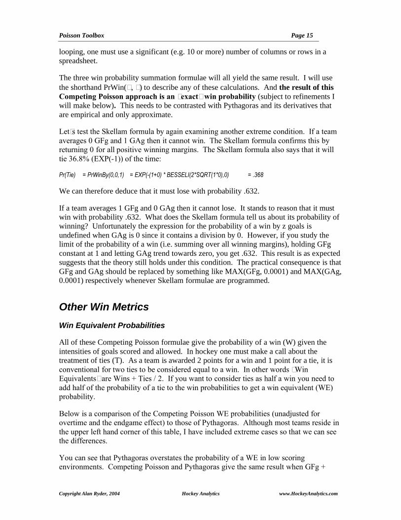
Let’s test the Skellam formula by again examining another extreme condition. If a team averages 0 GFg and 1 GAg then it cannot win. The Skellam formula confirms this by returning 0 for all positive winning margins. The Skellam formula also says that it will tie 36.8% (EXP(-1)) of the time:
Pr(Tie) = PrWinBy(0,0,1) = EXP(-(1+0) * BESSELI(2*SQRT(1*0),0) = .368
We can therefore deduce that it must lose with probability .632.
If a team averages 1 GFg and 0 GAg then it cannot lose. It stands to reason that it must win with probability .632. What does the Skellam formula tell us about its probability of winning? Unfortunately the expression for the probability of a win by z goals is undefined when GAg is 0 since it contains a division by 0. However, if you study the limit of the probability of a win (i.e. summing over all winning margins), holding GFg constant at 1 and letting GAg trend towards zero, you get .632. This result is as expected suggests that the theory still holds under this condition. The practical consequence is that GFg and GAg should be replaced by something like MAX(GFg, 0.0001) and MAX(GAg, 0.0001) respectively whenever Skellam formulae are programmed.
Other Win Metrics
Win Equivalent Probabilities
All of these Competing Poisson formulae give the probability of a win (W) given the intensities of goals scored and allowed. In hockey one must make a call about the treatment of ties (T). As a team is awarded 2 points for a win and 1 point for a tie, it is conventional for two ties to be considered equal to a win. In other words “Win Equivalents” are Wins + Ties / 2. If you want to consider ties as half a win you need to add half of the probability of a tie to the win probabilities to get a win equivalent (WE) probability.
Below is a comparison of the Competing Poisson WE probabilities (unadjusted for overtime and the endgame effect) to those of Pythagoras. Although most teams reside in the upper left hand corner of this table, I have included extreme cases so that we can see the differences.
You can see that Pythagoras overstates the probability of a WE in low scoring environments. Competing Poisson and Pythagoras give the same result when GFg +

Poisson Toolbox Page 16
Copyright Alan Ryder, 2004 Hockey Analytics www.HockeyAnalytics.com
GAg is about 6.5. For higher scoring environments, Pythagoras understates the probability of a WE. Below is a graph of these functions for GAg = 2.5.
These competing Poisson probabilities (not yet adjusted for overtime or the endgame effect) provide a better fit to the post WWII NHL data than does Pythagoras. The Poisson approach has an R-Square value of 94.1% while the R-Square of Pythagoras is 93.5%. This may not seem like such a large difference, but the state of the art is in chasing down these differences. The differences tend to arise in extreme cases as the preponderance of the data is in winning percentages between .300 and .700.
The major enhancement of Pythagoras has been due to (1) the recognition that a higher scoring context results in greater “resolution” in winning percentages and (2) the understanding that the right dynamic exponent (i.e. in the Pythagorean formula, replace the exponent 2 with a function of total scoring) gets you better resolution. A good team in a low scoring context is exposed to having bad luck turn a win into a loss or a tie. This is less so when scoring is higher. Better resolution is fundamentally why good basketball
Poisson vs Pythagoras (GAg = 2.5)
0.500 0.550 0.600 0.650 0.700 0.750 0.800 0.850 0.900 0.950 1.000
2 3 4 5 6 7 8Goals For per Game (GFg)
Win
Pro
babi
lity
PoissonPythagoras
Win Equivalent Probabilities
GAg GFg 2.5 3.0 3.5 4.0 5.0 6.0 7.0Poisson 0.500 0.583 0.656 0.719 0.818 0.887 0.931
2.5 Pythagoras 0.500 0.590 0.662 0.719 0.800 0.852 0.887Poisson 0.417 0.500 0.576 0.645 0.758 0.841 0.899
3.0 Pythagoras 0.410 0.500 0.576 0.640 0.735 0.800 0.845Poisson 0.344 0.424 0.500 0.571 0.695 0.790 0.860
3.5 Pythagoras 0.338 0.424 0.500 0.566 0.671 0.746 0.800Poisson 0.281 0.355 0.429 0.500 0.629 0.735 0.817
4.0 Pythagoras 0.281 0.360 0.434 0.500 0.610 0.692 0.754Poisson 0.182 0.242 0.305 0.371 0.500 0.617 0.717
5.0 Pythagoras 0.200 0.265 0.329 0.390 0.500 0.590 0.662Poisson 0.113 0.159 0.210 0.265 0.383 0.500 0.608
6.0 Pythagoras 0.148 0.200 0.254 0.308 0.410 0.500 0.576Poisson 0.069 0.101 0.140 0.183 0.283 0.392 0.500
7.0 Pythagoras 0.113 0.155 0.200 0.246 0.338 0.424 0.500

Poisson Toolbox Page 17
Copyright Alan Ryder, 2004 Hockey Analytics www.HockeyAnalytics.com
teams have really big winning percentages.
To the right is a comparison of Competing Poisson WE probabilities across scoring contexts. In this table I have held the ratio of GFg to GAg constant. As a result Pythagoras would always tell us that the win equivalent probability would be .610, roughly that of a 6.5 total goal context. You can see that the resolution of the Competing Poisson method does improve as the total scoring context increases. The theory predicts the reality.
Expected Points
The expected number of points is simply 2 x win equivalent probability. If a team has a win equivalent probability of .622 then it expected points would be 1.244 per game or 102 points in an 82 game season. If you award a point for an overtime loss expected points becomes:
Expected Points Per Game = 2 x WE Probability + Pr(OT Loss)
This finally gives us a tool to predict total points, bringing overtime losses into hockey analysis. I will discuss below how you can derive the probability of an overtime loss, but I will tell you right now that if you estimate points without OTLs and then add 4 points you are pretty much there.
Extensions of the Basic TheoryThe Question of Independence
So far I have assumed the independence of goals for and against. Making this assumption gives rise to what I have called “Competing Poisson” probabilities and the Skellam formula, PrWinBy(z, , ). The truth is that, if GF and GA are independent, there is no “competition” between them.
When we allow for the interdependence of GF and GA we get true Competing Poisson probabilities. If described the net propensity to score goals, described the netpropensity to allow goals and described the (additive only) effects of the interactions of and , then we would have a delicious conclusion. Under these circumstances of positive correlation of GF and GA, the probability distribution of the goal differential would be independent of . We would only have to choose the correct and to reflect the impact of . Unfortunately GF and GA are, if anything, negatively correlated.
The correlation coefficient of GFg and GAg, Cor(GAg,GAg), is a measurement of the degree of interaction in the variation of GFg and GAg. A correlation coefficient of +/-1 means that every change in GFg is accompanied by a perfectly predictable change in GAg. The sign indicates the direction of the change. For a negative correlation, it means
Win Equivalent Probabilities
GFg GAg Pr(WE) 1.250 1.000 0.562 1.875 1.500 0.578 2.500 2.000 0.591 3.125 2.500 0.602 3.750 3.000 0.612 4.375 3.500 0.621 5.000 4.000 0.629

Poisson Toolbox Page 18
Copyright Alan Ryder, 2004 Hockey Analytics www.HockeyAnalytics.com
that the two variables move in the opposite direction. A correlation of 0 means that the two variables are independent. In this case, a movement in one variable does not predict the movement of the other variable. A correlation of “near” zero is taken to imply the independence of the two variables. “Near” can be defined statistically. It depends on the amount of the data. A larger correlation is indicative of interdependence. The square of the correlation coefficient (“R-Square”) tells us the degree to which one variable explains the other variable (i.e. a correlation coefficient of 90% says that 81% of the movement of one variable is predicted by movement in the other). Covariance is a related index. It is simply the correlation coefficient measured in units of the variation in the data. Correlation and covariance will always have the same sign.
Hockey, at least today, is a negative correlation / covariance sport. Over the entire NHL this correlation is small but present (-.04 since 1999-00). Some, typically better, teams have an even larger (negative) correlation coefficient. Some teams have a positive correlation. Negative correlation of GF and GA means that, for a given team in a given game, there is a tendency for a “high” number of goals scored to be accompanied by a “low” number of goals allowed. Negative correlation means that teams “compete” for goals. It suggests a defensive mindset. This sounds like the NHL of today.
Soccer is a positive correlation / covariance sport. I think (I have not done the work) that basketball is a positive correlation sport. Positive correlation means that the pace of the game can be increased, expanding scoring for both teams. It suggests an offensive mindset. This may have been the case in earlier eras of the NHL. This correlation of GF and GA is, itself, highly correlated with the variation in total (GF + GA) scoring. When teams have a high variation in their total goals it is because they either want to or are easily forced to open up the game.
My conclusion that hockey, or at least half the league, has negative correlation calls into question our ability to simply adjust and downward. On the other hand, the math around a “negative ” is complex. We cannot simply increase and to account for the interactions.
Goals scored and allowed in hockey (i.e. over all teams) are “nearly” independent. And the reasons why we fail to observe the “theoretical” goal differential probabilities in hockey are, in a large way, a consequence of hockey’s quirks: the endgame and overtime. We are also generally interested only in the probability of a win or tie. Inaccuracies of a probability model for 2 or 3 goal wins don’t generally have consequences. For all of these reasons, I will leave the probability model as it is with only a couple of changes (see below) to reflect hockey’s quirks.
Regular Season Overtime
As discussed before, overtime distorts the Poisson probability of winning by turning games that would have resulted in a tie into games with a decision. To address the overtime problem one needs to look at the probability of winning and losing in overtime.

Poisson Toolbox Page 19
Copyright Alan Ryder, 2004 Hockey Analytics www.HockeyAnalytics.com
The probability of an overtime win is A x B x C, and the probability of an overtime loss is A x B x (1-C), where:
A. the probability of overtime
B. the probability of an overtime decision given that there is overtime
C. the probability of winning given that there is an overtime decision
A is simply the probability of a regulation tie. I developed a formula for that above and will enhance the formula when I consider the endgame effect.
For the current definition of overtime, B is equal to 1- the probability of neither team scoring within 5 minutes:
Pr(OT Decision) = 1- Pr(0 Goals) = 1- POISSON(0,OT + OT,FALSE) = 1 – EXP(-( OT + OT))
where OT and OT are 5/60ths of full (regulation) game propensities to score (i.e. GFg and GAg) adjusted for any changes in scoring propensity in overtime).
This may disappoint the Poisson fans out there, but C is determined as a one trial, Binomial process (coin toss) where the outcome probabilities are:
Pr(Win | OT Decision) = OT / (OT + OT)Pr(Loss | OT Decision) = OT / (OT + OT)
So the outcome probabilities, given overtime, are:
POTW = Pr(Win | Overtime) = OT / (OT + OT) x (1 – EXP(-( OT + OT)))POTL = Pr(Loss | Overtime) = OT / (OT + OT)x (1 – EXP(-( OT + OT)))
Finally we are in a position to modify the outcome probabilities to reflect regular season overtime:
Pr(Win by 1) = Pr(Regulation Win by 1) + Pr(Regulation Tie) x POTW
Pr(Win) = Pr(Regulation Win) + Pr(Regulation Tie) x POTW
the adjustment term being the probability of an overtime win.
Pr(Loss by 1) = Pr(Regulation Loss by 1) + Pr(Regulation Tie) x POTL
Pr(Loss) = Pr(Regulation Loss) + Pr(Regulation Tie) x POTL
the adjustment term being the probability of an overtime loss.
Pr(Tie) = Pr(Regulation Tie) x (1 – POTW – POTL)
the adjustment term being the probability of an overtime tie.

Poisson Toolbox Page 20
Copyright Alan Ryder, 2004 Hockey Analytics www.HockeyAnalytics.com
In 2004 there were 6618 goals scored including 145 in overtime. The average number of goals scored per team per game was 2.57 but this reduces to 2.51 in regulation time. So the first adjustment to make when one wants to consider overtime is to use a base and that reflect regulation time scoring propensities.
The correct OT and OT must also reflect the circumstances of overtime. Today each team removes a skater from the ice. And under today’s rules, although this is not the way most people think of it, teams entering the overtime period are both rewarded with a point for the regulation tie and what is at stake is a bonus point for an overtime win. The only risk of allowing an overtime goal is the foregone opportunity to claim the bonus point. Both of these circumstances mean that the rate of scoring is likely to increase. This is in fact the case.
In 2004, scoring (per minute) was about 143% of regulation scoring (since the current version of overtime was established, overtime scoring, per minute, has averaged 135% of regulation scoring). To get at OT and OT for individual teams is statistically challenging. You can certainly calculate it for a given team in a given season, but there will be considerable “noise” in the results. I prefer to make the assumption that, for any given team:
OT = (1+c) x / 12 OT = (1+c) x / 12
where c is constant across all teams. Assuming c = 43% and two average teams scoring and allowing 2.51 goals per regulation game (assumptions suitable for 2004), this theory says that regular season overtime should produce a decision 45% of the time. Assuming c = 36% and two average teams scoring and allowing 2.64 goals per regulation game (assumptions suitable for 2000-2004), this theory says that regular season overtime should also produce a decision 45% of the time. In 2004 (and since 1999-2000) overtime was, in fact, resolved in 46% of games.
Playoff Overtime
The probability of an overtime win in the playoffs is still A x B x C. But a deciding goal is always scored. That means B, the probability of an overtime decision, is always 1. If, as I have assumed above, OT and OT for a given team are the same multiple k of and then the probability C is insensitive to k. Consequently:
Pr(Win by 1) = Pr(Regulation Win by 1) + Pr(Regulation Tie) x / (+)
Pr(Playoff Win) = Pr(Regulation Win) + Pr(Regulation Tie) x / (+)
Pr(Loss by 1) = Pr(Regulation Loss by 1) + Pr(Regulation Tie) x / (+)
Pr(Playoff Loss) = Pr(Regulation Loss) + Pr(Regulation Tie) x / (+)
Pr(Tie) = 0, of course

Poisson Toolbox Page 21
Copyright Alan Ryder, 2004 Hockey Analytics www.HockeyAnalytics.com
Scoring tends to go down in the playoffs as teams tighten up defensively (a strategy that reduces winning resolution and typically favours the weaker team). As a consequence it is necessary to use a base and that reflect playoff scoring propensities.
Endgame Goals
The game can change in the closing minutes of regulation time. Teams trailing in a “close” game risk allowing an extra goal in order to increase the chance of generating an extra goal (or two) to obtain a tie. “Extra” goals in the last minutes of regulation time distort the Poisson probability of winning by changing the probabilities of a win by z. A 1 goal differential can become a 0 or 2 goal differential. Other goal differentials can be lessened or widened. I refer to this phenomenon as the “endgame effect”.
Unlike the case of overtime, a late goal does not end the game. So one way of looking at the endgame is to see it as a game within a game.
1 Goal Endgames
Let’s first examine the simplified case of a team trailing by one goal “late” in regulation play. The probability of an endgame when trailing is approximately PrWinBy(-1, , ), the probability of losing a regulation game by one goal. Notice that I have described this as approximate. For a one minute endgame an exact expression would be PrWinBy(-1, * 59/60, * 59/60). But as these two expressions produce very similar results, and the length of the endgame is uncertain, I will stick with the approximate expression.
In order to transform an impending loss into a regulation tie, the team needs to win the endgame by one goal. We have an expression for the probability of winning the trailing endgame by a goal given that there is a trailing endgame: PrWinBy(1, ET, ET).
The probability of a tie is increased by this amount. The probability of a loss (by 1) is reduced by this amount. Note that and need to be properly selected for the endgame conditions (time and scoring intensity) when trailing (hence I have labeled them ET and ET). It is nearly universal strategy to pull the goaltender when trailing by a goal in order to increase the . It therefore that case that, when trailing with one minute to play, ET >> /60 and ET > /60.
Of course, one can “lose” this endgame by a goal. That would increase the probability of 2 goal losses and reduce the probability of a 1 goal loss.
When leading by one goal late in regulation time (probability approximately = PrWinBy(1,,)) a team can “lose” the endgame by one goal with probability PrWinBy(-1,EL, EL). The probability of a tie is increased by this amount. The probability of a win (by 1) is reduced by this amount. When leading an endgame with one minute to play, EL >> /60 and EL > /60. And of course this endgame can be “won”, increasing the probability of 2 goal wins and reducing the probability of a 1 goal win.

Poisson Toolbox Page 22
Copyright Alan Ryder, 2004 Hockey Analytics www.HockeyAnalytics.com
In summary:
Goal Differential
Base Probability *
1 Goal DifferenceTrailing Adjustment
1 Goal DifferenceLeading Adjustment
-2 PrWinBy(-2,,) + PrWinBy(-1,,) x PrWinBy(-1,ET, ET)-1 PrWinBy(-1,,) x (1 - (PrWinBy(1,ET, ET) + PrWinBy(-1,ET, ET)))0 PrWinBy(0,,) + PrWinBy(-1,,) x PrWinBy(1,ET, ET) + PrWinBy(1,,) x PrWinBy(-1,EL, EL)1 PrWinBy(1,,) x (1 - (PrWinBy(1,EL, EL) + PrWinBy(-1,EL, EL)))2 PrWinBy(2,,) + PrWinBy(1,,) x PrWinBy(1,EL, EL)
Of course, these probabilities exclude the possibility of an endgame “win” (or loss) by 2 or more goals (e.g. scoring 2 goals when trailing by 1). Those probabilities are extremely remote and can be safely ignored in order to simplify the math. I have also assumed that all 1 goal games develop endgames. I think this is a safe assumption over most eras but the model can be adjusted to reduce the frequency of 1 goal endgames.
All of this can be generalized for an endgame of any length through the selection of the ’s and ’s. Earlier I demonstrated that the endgame seems to commence in the 19th
minute. In 2004, goals in the final two minutes of the third period were scored at the rate of about 200% of normal. I stated earlier that we would expect to see about 96 increases in lead and 96 decreases in lead the final two minutes. Instead we observed 125 (130% of normal) lead reductions and 258 (269% of normal) lead increases. Although we can get and by team, to get at ET, EL, ET and EL for individual teams is statistically challenging. One therefore might be inclined to conclude something like:
ET = 1.3 x / 30 ET = 2.7 x / 30EL = 2.7 x / 30 EL = 1.3 x / 30
Although it would fluctuate from season to season, I think that the factor reflecting empty net goals (270%) is not too bad. However, teams which are not in a “rallying” mode tend to be in a “given up” mode. The 30% increase in scoring when trailing is a combination of an increase due to the endgame effect and a decrease due to teams playing out the final minutes. In 2004 there were, in the final 2 minutes of regulation time, 68 lead reductions that tied the game. Assuming that all of these were “extra” goals, this is a rate of about 70% above normal scoring levels. Accordingly, I would be inclined to use endgame scoring factors of about 1.7 and 2.7 rather than 1.3 and 2.7.
The other parameter adjustment you need to make is to subtract these “extra” goals from regulation scoring propensities and . Part of this is easy – just subtract the empty net goals scored and allowed. This works team by team and across the league to adjust for the when-leading situation. The when-trailing part of this is harder. We have no summary record of endgame goals scored when trailing. In 2004, 315 games entered overtime. If 68 (21.6%) of those were a consequence of the endgame effect, we can estimate each team’s endgame goals scored /allowed when trailing based on their number of overtime games played and scoring propensities. For other seasons an estimate of league total endgame goals when trailing might be 20% of (T + OTW + OTL).

Poisson Toolbox Page 23
Copyright Alan Ryder, 2004 Hockey Analytics www.HockeyAnalytics.com
To the right is a table illustrating how you might do this for the 2004 season for Goals For (and below a similar analysis for Goals Against). Note that the normalized rate of scoring is about 7% less than the nominal rate.
OTW, OTL and OTGP are overtime wins (goals for), losses (goals against) and games played respectively.
GFgR (GAgR) represents the goals for (against) rate in regulation time (i.e. with overtime goals removed).
GFEGt is the estimated (and therefore fractional) number of endgame goals scored when trailing (GAEGl is estimated endgame goals against when leading).
GFgN (GagN) represents the normalized goals for (against) rate after backing out the endgame effects.
The effects of these adjustments to and are subtle but have the potential to move the 2nd or 3rd significant digit in any given win / tie probability estimate.
2 Goal Endgames
As there is nothing to lose, the odds do not stop coaches from pulling the goaltender when down by two or more goals (recall that in 2004 there were 90 empty net goals that occurred when a team trailed by 2 or more goals). Even assuming that the goaltender remains in the net for all endgames of a more than 2 goal differential, this still distorts the probability of a win/loss by 1, 2 and 3 goals.
2004 Goals For Propensities
Team GFg OTW GFgR OTGP GFEGt GFEN GFgNANA 2.24 4 2.20 22 2.09 4 2.12ATL 2.61 6 2.54 18 1.97 6 2.44BOS 2.55 8 2.45 30 3.18 6 2.34BUF 2.68 2 2.66 13 1.49 10 2.52CAL 2.44 3 2.40 13 1.35 9 2.28CAR 2.10 5 2.04 25 2.20 4 1.96CBJ 2.16 6 2.09 18 1.62 4 2.02CHI 2.29 4 2.24 23 2.23 2 2.19COL 2.88 8 2.78 28 3.36 6 2.67DAL 2.37 3 2.33 18 1.81 5 2.25DET 3.11 7 3.02 20 2.61 8 2.89EDM 2.70 6 2.62 23 2.60 5 2.53FLA 2.29 5 2.23 24 2.31 3 2.17LA 2.50 2 2.48 27 2.89 6 2.37MIN 2.29 1 2.28 24 2.36 5 2.19MON 2.54 5 2.48 16 1.71 10 2.33NAS 2.63 7 2.55 22 2.42 4 2.47NJD 2.60 7 2.51 21 2.28 5 2.42NYI 2.89 2 2.87 17 2.10 12 2.69NYR 2.51 3 2.48 18 1.92 7 2.37OTT 3.20 3 3.16 19 2.59 12 2.98PHI 2.79 2 2.77 23 2.75 7 2.65PHO 2.29 5 2.23 29 2.80 4 2.15PIT 2.32 7 2.23 19 1.83 2 2.18SJ 2.67 3 2.63 21 2.39 6 2.53STL 2.33 11 2.20 24 2.28 9 2.06TB 2.99 4 2.94 18 2.28 10 2.79TOR 2.95 4 2.90 17 2.13 11 2.74VAN 2.87 11 2.73 26 3.07 4 2.65WAS 2.27 1 2.26 14 1.36 3 2.20Total 145 630 68 189Avg 2.57 4.83 2.51 21.00 2.27 6.30 2.40

Poisson Toolbox Page 24
Copyright Alan Ryder, 2004 Hockey Analytics www.HockeyAnalytics.com
If you care about a better representation of the probability of a win by z goals, you need to consider 2 goal endgames. If all you are interested in is the probability of a win, tie or loss (and you are prepared to assume that 2 goal endgames cannot result in a tie), then there is no benefit to extending the calculations.
I am normally not concerned with anything other than the probability of a win, tie or loss. But, if you are so inclined, the extension of these calculations is easy to address by repeating the process used for one-goal endgames. Some two goal wins / losses are transformed into 3 or 1 goal wins / losses. In 2004, only 4 times did a team rally from a 2 goal deficit to tie a game. As the math is already approximate, I think that it is safe to ignore this possibility.
To combine both the 1 goal and 2 goal endgames first make the 1 goal adjustments above, then make the following adjustments:
Goal Differential
Base Probability *
2 Goal DifferenceTrailing Adjustment
2 Goal DifferenceLeading Adjustment
-3 PrWinBy(-3,,) + PrWinBy(-2,,) x PrWinBy(-1,ET, ET)-2 PrWinBy(-2,,) x (1 - (PrWinBy(1,ET, ET) + PrWinBy(-1,ET, ET)))-1 PrWinBy(-1,,) + PrWinBy(-2,,) x PrWinBy(1,ET, ET)0 PrWinBy(0,,)1 PrWinBy(1,,) + PrWinBy(2,,) x PrWinBy(-1,EL, EL)2 PrWinBy(2,,) x (1 - (PrWinBy(1,EL, EL) + PrWinBy(-1,EL, EL)))3 PrWinBy(3,,) + PrWinBy(2,,) x PrWinBy(1,EL, EL)
This assumes that all 2 goal games develop endgames. This assumption might be realistic today, but was less so in the past when fewer 2 goal deficits were attacked in this fashion. It is a simple matter to change the model to reflect the frequency of 2 goal endgames
2004 Goals Allowed Propensities
Team GAg OTL GAgR OTGP GAEGl GAEN GAgNANA 2.60 8 2.50 22 2.37 7 2.39ATL 2.96 4 2.91 18 2.26 14 2.72BOS 2.29 7 2.21 30 2.86 4 2.12BUF 2.70 4 2.65 13 1.49 4 2.58CAL 2.15 3 2.11 13 1.18 8 2.00CAR 2.55 6 2.48 25 2.67 8 2.35CBJ 2.90 4 2.85 18 2.22 10 2.70CHI 3.16 8 3.06 23 3.04 11 2.89COL 2.41 7 2.33 28 2.82 7 2.21DAL 2.13 2 2.11 18 1.64 6 2.02DET 2.30 2 2.28 20 1.97 6 2.18EDM 2.54 5 2.48 23 2.46 3 2.41FLA 2.70 4 2.65 24 2.74 7 2.53LA 2.65 9 2.54 27 2.96 10 2.38MIN 2.23 3 2.20 24 2.27 4 2.12MON 2.34 4 2.29 16 1.58 4 2.22NAS 2.65 4 2.60 22 2.47 12 2.42NJD 2.00 2 1.98 21 1.79 4 1.90NYI 2.56 4 2.51 17 1.84 1 2.48NYR 3.05 8 2.95 18 2.29 4 2.87OTT 2.30 6 2.23 19 1.83 3 2.17PHI 2.27 6 2.20 23 2.18 2 2.14PHO 2.99 6 2.91 29 3.65 8 2.77PIT 3.70 4 3.65 19 2.99 13 3.45SJ 2.23 6 2.16 21 1.96 3 2.10STL 2.41 2 2.39 24 2.48 5 2.30TB 2.34 6 2.27 18 1.76 7 2.16TOR 2.49 3 2.45 17 1.80 3 2.39VAN 2.37 5 2.30 26 2.59 2 2.25WAS 3.09 3 3.05 14 1.84 9 2.92Total 145 630 68 189Avg 2.57 4.83 2.51 21.00 2.27 6.30 2.40

Poisson Toolbox Page 25
Copyright Alan Ryder, 2004 Hockey Analytics www.HockeyAnalytics.com
Another Approach
As a practical matter, a goal usually ends the endgame. That suggests that we can adapt the Trinomial model used for overtime. This approach is a little less computationally intense and I therefore prefer it. As above, we need to consider two scenarios, trailing and leading. And I will only address the probabilities of wins, ties and losses.
When trailing the probability of scoring an endgame goal and transforming an impending loss into a tie is A x B x C where:
A. the probability of a trailing endgame
B. the probability of a goal by either team given a trailing endgame
C. the probability of scoring the goal given an endgame goal
The probability of a trailing endgame is approximately:
A = PrWinBy(-1, , ).
The probability of a goal during a trailing endgame is:
B = Pr(Endgame Goal) = 1- Pr(0 Goals) = 1- POISSON(0, ET + ET,FALSE) = 1- EXP(- ET - ET)
C is determined as a one trial Binomial process (coin toss) where the outcome probabilities are:
C = Pr(Goal Scored |Endgame Goal) = ET / ( ET + ET)
When leading the probability of allowing an endgame goal and transforming an impending win into a tie is A x B x C where:
A. the probability of a leading endgame
B. the probability of a goal by either team given a leading endgame
C. the probability of allowing the goal given an endgame goal
The probability of a leading endgame is approximately:
A = PrWinBy(1, , ).
Given the proper and , the probability of a goal during a trailing endgame is:
B = Pr(Endgame Goal) = 1- Pr(0 Goals) = 1- POISSON(0, EL + EL,FALSE) = 1- EXP(- EL - EL)
C is determined as a one trial Binomial process (coin toss) where the outcome probabilities are:
C = Pr(Goal Allowed |Endgame Goal) = EL / ( EL + EL)

Poisson Toolbox Page 26
Copyright Alan Ryder, 2004 Hockey Analytics www.HockeyAnalytics.com
Using this model, the revised probabilities are (approximately):
Pr(Regulation Win) = PrWin(,) - PrWinBy(1,,)) x (1 - EXP(EL, EL)) x EL / ( EL + EL)
the adjustment term being the probability of a blown lead in an endgame.
Pr(Regulation Loss) = PrLoss(,) - PrWinBy(-1,,)) x (1 - EXP(ET, ET)) x ET / ( ET + ET)
the adjustment term being the probability of tying the game in the final moments.
Pr(Regulation Tie) = PrWinBy(0,,) + PrWinBy(1,,)) x (1 - EXP(EL, EL)) x EL / ( EL + EL)+ PrWinBy(-1,,)) x (1 - EXP(ET, ET)) x ET / ( ET + ET)
the adjustment term being the probability of a tie due to the endgame effect.
What are the right ’s and ’s? They would be, as before, something like:
ET = 1.7 x / 30 ET = 2.7 x / 30EL = 2.7 x / 30 EL = 1.7 x / 30
Extended Competing Poisson Example
To put this all together, let’s look at Pittsburgh in 2004. The Penguins had a record of 23-51-8 for 58 points (4 OTLs) and a .329 win equivalent percentage.
The Penguins scored 190 goals and allowed 303 in 2004. Pythagoras estimates their win equivalent probability at .282. The PythagenPuck (normally more accurate) estimate is .257. This was a bad team.
Pittsburgh’s season scoring translates to 2.32 GFg and 3.70 GAg. The basic Competing Poisson (ignoring overtime and the endgame) estimate for the win equivalent probability is .290.
The Penguins were a very lucky 7 and 4 in OT decisions. This made their regulation time scoring propensities 2.23 (for) and 3.65 (against). They gave up 13 empty net goals and scored only 2. Their estimated and , normalized for the endgame, are 2.18 and 3.45 respectively. Using PrWin(2.18, 3.45, 0, 0, 1.7/30, 2.7/30, 0.4, 2, 3) (see Appendix) we get a better Pr(WE) estimate of .283 and the results displayed to the right.
Notice the random “noise” introduced by a limited number of sudden death overtimes in which Pittsburgh was either lucky or skillful. The Penguins played in 19 overtimes going 7 – 4 – 8. If Pittsburgh had gone 3 – 4 – 12 in overtime (expected record given 19 regulation
Pittsburgh’s Probabilities
Per Game
Full Season
Win .217 18Loss (including OT) .651 53Tie .132 11
WE .283 23Expected Points .641 53

Poisson Toolbox Page 27
Copyright Alan Ryder, 2004 Hockey Analytics www.HockeyAnalytics.com
ties) they would have ended the season with 54 points on 19 wins, 51 losses and 12 ties. This is an awfully good fit with the Competing Poisson model.
Head to Head Match UpsTo assess a team’s winning expectations one pits its propensity to score goals against its propensity to allow them. I refer to win probabilities determined in this fashion as Competing Poisson probabilities. Implicit, so far, is the assumption that the team in question is facing an unknown or neutral (i.e. average) opponent. But what if it is not?
When two .600 teams play each other, it is easy to conclude that each team has a 50% chance of success. But what about when a .750 team plays a 600 team?
The conventional wisdom is to imagine simultaneously tossing two “unfair” coins. Coin A has the probability of turning up heads 75% of the time, and Coin B has the probability of turning up heads 60% of the time. Toss the coins. If two heads or two tails show up, the contest is a push and you need to toss again. Once you get one head and one tail, the contest is over and the winner is the head.
If you toss the coins once there are four possible outcomes:
In 55% of the cases you will need to toss the coins again. But the rest of the time you will get a winner with Coin A winning in 30% if the tosses and Coin B winning in 15%. That means that the probability of A being the winner of this contest is .30 / (.30 + .15).
In general, when there must be a winner:
Pr(A beats B) = A x (1-B) / (Ax (1-B) + B x (1-A))
This thought process works when there are only two outcomes. Treating a tie as half a win fails us here. Since we have competing forces at work for goals scored and allowed, we can develop a more rigorous approach by the application of Competing Poisson probabilities:
Let GFg< = League Average Goals per Game ( = GAg<)GFgX = Average Goals For per Game for Team XGAgX = Average Goals Against per Game for Team X
Coin Toss Probabilities
Coin A H T H TCoin B H T T HProbability .45 = .75 x .60 .10 = .25 x .40 .30 = .75 x .40 .15 = .25 x .60

Poisson Toolbox Page 28
Copyright Alan Ryder, 2004 Hockey Analytics www.HockeyAnalytics.com
Then, for Team A = GFgA x GAgB / GFg< = GAgA x GFgB / GFg<
Pr(Tie) = PrWinBy(0,,)
Pr(A Wins) = k PrWinBy(k,,),k = 1, 2, 3, …
For more accuracy, one would use the extended Competing Poisson method. For Team B, and are simply reversed.
To the right is a comparison of two teams (A and B) that are predicted by the Competing Poisson method to have WE probabilities of .623 and .600 respectively. Team A has a total scoring context of 7.19 goals per game while Team B has a total scoring context of 4.80 goals per game (league average scoring context is assumed to be 5.14 goals per game as it was in 2004). I created this example to have the ratio of (GFg) to (GAg) be the same for the two teams and the result is that these two teams are now seen to be evenly matched (head to head) notwithstanding Team A’s apparent (WE) superiority.
The conventional head to head approach, using WE probabilities, would have told you that Team A should win more often. But the Competing Poisson approach says that the two teams are evenly matched. This is the correct conclusion and suggests that the relevance of scoring context disappears in a head-to-head analysis.
The second example is real: Tampa Bay versus Calgary in 2004. The Lightning lived in a slightly higher than league average scoring context (5.33 goals per game) while the Flames were quite a bit below average (4.59). This analysis says that Tampa wins with probability .455, Calgary wins with probability .357 and .188 of the games result in a regulation tie (using the basic Competing Poisson method). The Win Equivalent probability is therefore .549 in favour of the Lightning, ignoring the matter of home ice advantage.
Competing Teams, Example 1
Team A Team B Team A (vs B) GFg< 2.57
4.024 2.683 3.314 3.170 2.113 3.314
Pr(T) 0.145 0.182 0.158Pr(W) 0.550 0.509 0.421
Pr(WE) 0.623 0.600 0.500
Competing Teams, Example 2
Tampa Bay Calgary TB (vs CAL)GFg< 2.57
2.988 2.439 2.499 2.341 2.146 2.225
Pr(T) 0.171 0.191 0.188Pr(W) 0.522 0.457 0.455
Pr(WE) 0.608 0.553 0.549Pr(PW) 0.554

Poisson Toolbox Page 29
Copyright Alan Ryder, 2004 Hockey Analytics www.HockeyAnalytics.com
In the playoffs, games cannot end in a tie. With Competing Poisson processes you can model the overtime outcome as a one-trial Binomial process with the probability of a Tampa win, given overtime, of 2.499 / (2.499 + 2.225) = .529. So the Playoff Win (PW) probability for Tampa Bay is .458 + .188 x .529 = .554 (ignoring home ice). Note that this is larger than the WE probability (.549) due to the increased resolution of overtime. If you use the extended Competing Poisson method the Pr(PW) is a bit larger.
Just to finish with this example (I am continuing to ignore home ice and the math here is Binomial rather than Poisson), the series opening probability of a Lightning Stanley Cup victory over Calgary was .617 (see table to right). This is higher than Tampa’s PW probability because of the increased resolution of a 7 game series.The Flames and Bolts traded wins until game 7. As the underdogs, Calgary’s chances improved as they lengthened the series (see second table). Going into game 6, Tampa Bay needed two consecutive wins (probability .307) to collect the Cup. Going into game 7, since the series had been reduced to a single game, Tampa’s win probability was .554. In the end, the better team won.
Home Ice Advantage
Home ice tends to increase home team scoring by about 5% and reduce visitor scoring by a similar amount. I am sure that this relationship has varied over time, but a quick and dirty way to adjust for home ice is to adjust and :
= 1.05 x
= / 1.05
With today’s scoring context the difference works out to a quarter of a puck and, when we match two average teams, that translates to a .544 win equivalent probability (for an average home team versus an average visitor). Given Tampa’s home ice advantage in game 7, their win probability was more like .599.
Initial Series Win Probabilities
SeriesLength Tampa Bay Calgary
4 0.094 0.0405 0.168 0.0886 0.187 0.1217 0.167 0.134
Total 0.617 0.383
Series Win Probabilities
Before Game … Tampa Bay Calgary
1 0.617 0.3832 0.450 0.5503 0.601 0.3994 0.398 0.6025 0.581 0.4196 0.307 0.6937 0.554 0.446

Poisson Toolbox Page 30
Copyright Alan Ryder, 2004 Hockey Analytics www.HockeyAnalytics.com
State Expectations: Outcome Probabilities During a GameSo far I have been discussing outcome probabilities under the assumption that the game has not yet commenced. Once a game has started, two other factors come into play:
There may be a part score. For example, consider a team trailing by a goal. A tie now requires outscoring the opposition by one goal over the remainder of the game. A win requires outscoring the opposition by two or more goals over the remainder of the game. When trailing, the road is uphill.
The time remaining to score (or allow) goals reduces as the game progresses. This means that gets smaller as the game progresses. Remember that is sometimes expressed as λt where t is the time period under consideration. Up until now, I have been assuming t = 1 game. Once we are half way through the game, t has become ½ and we have exhausted half our total scoring expectation. When trailing, the uphill road is into a headwind.
The probability of a tie when trailing by m goals is the same as the probability of winning by m goals when tied. Both require that the opposition be outscored by m goals over the remainder of the game. In general the probability of a tie given a lead of m goals is:
Pr(Tie | Leading by m) = PrWinBy(-m, t, t)
Here and are as previously defined and t represents the percentage of the game that is remaining (eg t = 1/3 after two periods).
The probability of a win when trailing by m goals at time t is the same as the probability of winning by m or more goals when tied at time t. Both require that the opposition be outscored by m or more goals over the remainder of the game. Here is the probability:
Pr(Win | Trailing by m) = k PrWinBy(k, t, t), k = m+1, m+2, ...
The probability of a win when leading by m goals at time t is 1 – the probability of losing by m or more goals when tied at time t. The opposition must outscore by m or more goals over the remainder of the game.
Pr(Win | Leading by m) = 1 - k PrWinBy(k, t, t), k = -m-1, -m-2, ...
One can therefore use Competing Poisson probabilities within a game to determine the “potential energy” of a given “state” of the game (the “state expectations”). By potential energy I mean the win equivalent (or similar) expectation. By state I mean the goal differential and the elapsed or remaining time in the game.

Poisson Toolbox Page 31
Copyright Alan Ryder, 2004 Hockey Analytics www.HockeyAnalytics.com
Below is a graph that shows these win equivalent state expectations, ignoring overtime, for a team averaging 3 goals for and 2.5 goals against per game.
This team commences the game with a win equivalent state value (WESV) of .583, its win equivalent probability. As long as the game remains scoreless, the WESV drifts downwards towards .500. This team is expected to win more often than lose. Skating in a tie game is increasingly a disappointment for the team.
This gives us a way of evaluating the impact of events in a game. All game events theoretically change the WESV. The first kind of event you would want to study is goal scoring, but you could advance this to penalties and even, with the right supporting data, to events like turnovers. Let’s look at a way that you might employ WESVs using the following scoring scenario:
Period Time State WESV Change Comment1 0:00 Tied .583 WE Probability1 10:15 Tied .575 -.008 10 minutes of tied hockey1 10:16 Up 1-0 .746 +.171 Early go ahead goal. 75% WE probability1 19:48 Up 1-0 .757 +.011 10 minutes of hockey up 1 goal1 19:49 Tied 1-1 .567 -.190 Blown lead2 4:50 Tied 1-1 .562 -.005 5 minutes of tied hockey2 4:51 Down 2-1 .340 -.222 Down 12 9:48 Down 2-1 .321 -.019 5 minutes of hockey down 12 9:49 Tied 2-2 .557 +.236 Back to an even score2 15:13 Tied 2-2 .551 -.006 5 minutes of tied hockey2 15:14 Up 3-2 .790 +.239 Up 1. Second period go ahead goal.2 19:39 Up 3-2 .805 +.015 5 minutes of hockey up 12 19:40 Up 4-2 .940 +.135 Up 2. 94% WE probability3 5:04 Up 4-2 .958 +.018 5 minutes of hockey up 23 5:05 Up 4-3 .835 -.123 Third Period goal cuts lead from 2 to 13 20:00 Win 4-3 1.000 +.165 15 minutes protecting 1 goal lead
Win Equivalent Expectations
0.0000.1000.2000.3000.4000.5000.6000.7000.8000.9001.000
0 10 20 30 40 50 60
Time
Down 4Down 3Down 2Down 1TiedUp 1Up 2Up 3Up 4

Poisson Toolbox Page 32
Copyright Alan Ryder, 2004 Hockey Analytics www.HockeyAnalytics.com
Note that:
when the game was “close”, the value of goals increased as the game progressed.
the goal that created the 2 goal lead was worth less even though it was later in the game.
playing with a lead increased expectation, playing while behind reduced WESV and playing tied (for this team) reduced WESV.
protecting a one goal lead in the third period was about as valuable to this team as scoring the first goal.
SummaryHockey is basically Poisson. It has a few quirks, but they can be addressed. What about the other major team sports? Soccer is Poisson. The game is essentially the same. Basketball is not Poisson. Scoring is not rare. In effect, each team takes turns shooting with a multinomial outcome (0,1,2,or 3 points). Football might be nearly Poisson. Scoring is random, rare and probably as memoryless as hockey. The problem is that there are at least two ways to score. Baseball may be “Poisson enough” (it might pass a Chi-Square goodness of fit test). But, on theoretical grounds, I think that it has some Poisson problems. Because Baseball is a Markov chain, I don’t think that scoring can be thought of as memoryless. Zero run innings occur disproportionately. The run potential of an inning builds as runners get on base. The scoring of one run suggests the potential for more runs. In addition, the game ends early when the home side is ahead after 8.5 innings and is extended whenever the game is tied at the end of an inning >8. But these issues may be no greater than hockey’s quirks.
Here are the key conclusions from this tour through the Poisson distribution.
1. Goal scoring in hockey is a Poisson process. The presence of regulation overtime, as it is currently defined, does not materially affect this conclusion. The scoring frenzy of the last minutes of the third period, however, does violate the Poisson premise. But one can address both of these quirks.
2. The number of goals scored in a hockey game follows the Poisson distribution. In Excel, the probability of a team, averaging goals scored per game, scoring k goals in a game is expressed in Excel as
POISSON(k, , FALSE)
and the probability of scoring k or fewer goals in a game is expressed as
POISSON(k, , TRUE)

Poisson Toolbox Page 33
Copyright Alan Ryder, 2004 Hockey Analytics www.HockeyAnalytics.com
and the probability of scoring more than k goals in a game is expressed as
1- POISSON(k, , TRUE)
3. The number of goals allowed in a hockey game is also Poisson. The expression for the probability of a team allowing k, more than k, or k or fewer goals in a game is as above, with replaced by , the average number of goals allowed per game.
4. Goals for and against appear to be statistically independent variables. More work needs to be done on this assertion.
5. The probability of winning a regulation game by z goals is given by the Competing Poisson expression (in Excel):
PrWinBy(z, , ) = EXP(-(+) * (/)^(z/2) * BESSELI(2*SQRT(*),ABS(z)).
where is GFg (Goals For per Game) and is GAg (Goals Against per Game). This holds for all z including negative values (losses) and 0 (ties). This probability ignores the endgame effect and overtime.
6. The probability of a win in regulation time (PrWin) is
k PrWinBy (k, , ), k= 1, 2, 3, …., or
m (e- x m / m!) x k (e- x k/k!), m = 1, 2, …, k = 0, 1, 2, …, m-1
This probability ignores the endgame effect and overtime. In practice these summation iteration may be terminated when the incremental probability becomes smaller than some tolerance. See Appendix for Visual Basic coding of the second expression.
7. Win Equivalents (WE) are defined as Wins + Ties / 2. The probability of a Win Equivalent is:
Pr(Win) + Pr(Tie) / 2
8. Expected Points per game are:
2 x Pr(Win) + Pr(Tie) + Pr(Regulation Tie) x (1 – EXP(-( OT + OT))) x OT / (OT + OT)
9. The basic Competing Poisson method can be extended to approximately address the endgame effect:
Pr(Regulation Win) = PrWin(,) - PrWinBy(1,,)) x (1 - EXP(EL, EL)) x EL / ( EL + EL)
Pr(Regulation Loss) = PrLoss(,) - PrWinBy(-1,,)) x (1 - EXP(ET, ET)) x ET / ( ET + ET)
Pr(Regulation Tie) = PrWinBy(0,,) + PrWinBy(1,,)) x (1 - EXP(EL, EL)) x EL / ( EL + EL)+ PrWinBy(-1,,)) x (1 - EXP(ET, ET)) x ET / ( ET + ET)

Poisson Toolbox Page 34
Copyright Alan Ryder, 2004 Hockey Analytics www.HockeyAnalytics.com
and to exactly address regular season overtime:
Pr(Win) = Pr(Regulation Win) + Pr(Regulation Tie) x (1 – EXP(-( OT + OT))) x OT / (OT + OT)
Pr(Loss) = Pr(Regulation Loss) + Pr(Regulation Tie) x (1 – EXP(-( OT + OT))) x OT / (OT + OT)
Pr(Tie) = Pr(Regulation Tie) x EXP(-( OT + OT))
10. The probability of a playoff win (PW) is:
Pr(Regulation Win) + Pr(Regulation Tie) x / ( +)
11. When two specific teams (A and B) compete, the regulation outcome probabilities of Team A are also determined by the PrWin and PrWinBy expressions with
= GFgA x GAgB / GFg< = GAgA x GFgB / GFg<
For Team B outcome probabilities, reverse and .
12. When two specific teams (A and B) compete in the playoffs, games cannot end in a tie. The probability of a Playoff Win for Team A is
Pr(Win) + Pr(Tie) x / ( + )
where and are as defined in (11).
13. To determine the probability of a team winning a 7 game playoff series, sum the probabilities if winning in 4, 5, 6 and 7 games. For a team with playoff win probability PW, the probability of winning a playoff series in z games is
PW4 x (1 - PW)(z-4) x (z-1)! / (3! x (z-4)!)
14. To determine the probability of win, tie or win equivalent within a game, adjust the and to reflect the remaining time and reflect the current score by translating the problem to an equivalent one involving winning or losing by the current goal differential:
Pr(Tie | Trailing by m) = PrWinBy(m, t, t))
Pr(Tie | Leading by m) = PrWinBy(-m, t, t))
Pr(Win | Trailing by m) = k PrWinBy(k, t, t), k = m+1, m+2, ...
Pr(Win | Leading by m) = 1 - k PrWinBy(k, t, t), k = -m-1, -m-2, ...
t = percentage of game remaining

Poisson Toolbox Page 35
Copyright Alan Ryder, 2004 Hockey Analytics www.HockeyAnalytics.com
15. Take care in selecting the parameters and . Adjust as required for:
Home ice advantage.
For and , the endgame effect, by removing (excess) endgame goals, and overtime, by removing overtime goals.
For EL , EL , ET and ET to reflect the small amount of time remaining and the significantly altered goal scoring intensities.
For OT and OT to reflect the length of overtime and the altered goal scoring intensities.
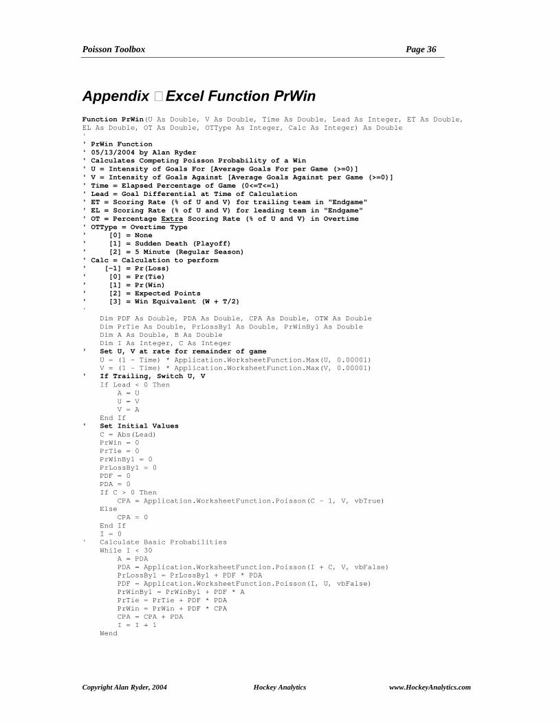
Poisson Toolbox Page 36
Copyright Alan Ryder, 2004 Hockey Analytics www.HockeyAnalytics.com
Appendix – Excel Function PrWinFunction PrWin(U As Double, V As Double, Time As Double, Lead As Integer, ET As Double,
EL As Double, OT As Double, OTType As Integer, Calc As Integer) As Double
'
' PrWin Function
' 05/13/2004 by Alan Ryder
' Calculates Competing Poisson Probability of a Win
' U = Intensity of Goals For [Average Goals For per Game (>=0)]
' V = Intensity of Goals Against [Average Goals Against per Game (>=0)]
' Time = Elapsed Percentage of Game (0<=T<=1)
' Lead = Goal Differential at Time of Calculation
' ET = Scoring Rate (% of U and V) for trailing team in "Endgame"
' EL = Scoring Rate (% of U and V) for leading team in "Endgame"
' OT = Percentage Extra Scoring Rate (% of U and V) in Overtime
' OTType = Overtime Type
' [0] = None
' [1] = Sudden Death (Playoff)
' [2] = 5 Minute (Regular Season)
' Calc = Calculation to perform
' [-1] = Pr(Loss)
' [0] = Pr(Tie)
' [1] = Pr(Win)
' [2] = Expected Points
' [3] = Win Equivalent (W + T/2)
'
Dim PDF As Double, PDA As Double, CPA As Double, OTW As Double
Dim PrTie As Double, PrLossBy1 As Double, PrWinBy1 As Double
Dim A As Double, B As Double
Dim I As Integer, C As Integer
' Set U, V at rate for remainder of game
U = (1 - Time) * Application.WorksheetFunction.Max(U, 0.00001)
V = (1 - Time) * Application.WorksheetFunction.Max(V, 0.00001)
' If Trailing, Switch U, V
If Lead < 0 Then
A = U
U = V
V = A
End If
' Set Initial Values
C = Abs(Lead)
PrWin = 0
PrTie = 0
PrWinBy1 = 0
PrLossBy1 = 0
PDF = 0
PDA = 0
If C > 0 Then
CPA = Application.WorksheetFunction.Poisson(C - 1, V, vbTrue)
Else
CPA = 0
End If
I = 0
' Calculate Basic Probabilities
While I < 30
A = PDA
PDA = Application.WorksheetFunction.Poisson(I + C, V, vbFalse)
PrLossBy1 = PrLossBy1 + PDF * PDA
PDF = Application.WorksheetFunction.Poisson(I, U, vbFalse)
PrWinBy1 = PrWinBy1 + PDF * A
PrTie = PrTie + PDF * PDA
PrWin = PrWin + PDF * CPA
CPA = CPA + PDA
I = I + 1
Wend

Poisson Toolbox Page 37
Copyright Alan Ryder, 2004 Hockey Analytics www.HockeyAnalytics.com
' Restore Full Game Intensities
U = U / (1 - Time)
V = V / (1 - Time)
' Endgame Goals: Some Losses Become Ties, Some Wins Become Ties
If ET > 0 Then
A = PrWinBy1 * (1 - Exp(-U * EL - V * ET)) * V * ET / (U * EL + V * ET)
B = PrLossBy1 * (1 - Exp(-U * ET - V * EL)) * U * ET / (U * ET + V * EL)
PrWin = PrWin - A
PrTie = PrTie + A + B
End If
' If Trailing calculations were reversed
If Lead < 0 Then PrWin = 1 - PrWin - PrTie
' Adjust for Overtime
If OTType = 2 Then
A = (1 - Exp(-(U + V) * (1 + OT) / 12))
Else
A = OTType
End If
OTW = U / (U + V)
B = PrTie * A
PrWin = PrWin + B * OTW
PrTie = PrTie - B
If OTType = 1 Then B = 0
' Pr(Loss)
If Calc = -1 Then PrWin = 1 - PrWin - PrTie
' Pr(Tie)
If Calc = 0 Then PrWin = PrTie
' Expected Points
If Calc = 2 Then PrWin = 2 * PrWin + PrTie + B * (1 - OTW)
' Pr(Win Equivalent)
If Calc = 3 Then PrWin = PrWin + 0.5 * PrTie
End Function


![IBFD Publications Style and Spelling Guidelines · 2018. 12. 7. · Dashes/hyphens X For word breaks: use hyphens [-]. X For dashes use en-dashes [–] (= ctrl + minus symbol in numerical](https://img.dokumen.tips/doc/110x75/5fc00d385740b25ae36a1d36/ibfd-publications-style-and-spelling-guidelines-2018-12-7-dasheshyphens-x.jpg)


